pr al network confer ,v - west virginia universitycommunity.wvu.edu/~hhammar/main.pdf · ergence...
TRANSCRIPT

[20] M. Witbrock and M. Zagha, \Backpropagation learning on the IBM GF 11", in Parallel Digital
Implementation of Neural Networks, pp.77-104, 1993.
[21] H. Yoon and J.H. Nang \Multilayer neural networks on distributed-memory multiprocessors",
Proceedings of International Neural Network Conference, Vol.2, pp.669-672, 1990.
[22] S. Zeng, \The Application of Parallel Processing Techniques to Neural Network Based Fingerprint
Recognition Systems", Thesis, Department of Electrical and Computer Engineering, West Virginia
University, 1994.
[23] X. Zhang, M. Mckenna, J.F. Mesirov and D. Waltz, \An e�cient implementation of the backpro-
pogation algorithm on the Connection Machine CM-2", in Parallel Computing, Vol.14, pp.317-327,
1990.
20

[4] E.M. Deprit, \Implementing recurrent back-propagation on the Connection Machine", in Neural
Networks, Vol.2, pp.295-314, 1989.
[5] F. Distante, M. Sami, R. Stefanelli and G. Storti-Gajani, \Mapping neural nets onto a massively
parallel architecture: a defect-tolerance solution", in Proceedings of The IEEE, Vol.79, pp.444-460,
October 1991.
[6] S.K. Foo, P. Saratchandran and N. Sundararajan, \Analysis of training set parallelism for back-
propagation neural networks", in International Journal of Neural Systems, Vol.6, pp.61-78, 1995.
[7] Y. Fujimoto, N. Fukuda and T. Alcabane, \Massively parallel architectures for large scale neural
network simulations", in IEEE Transactions on Neural Networks, Vol.3, pp.876-888, November
1992.
[8] S. Haykin, Neural Networks, a Comprehensive Foundation, Macmillan, 1994.
[9] K. Hwang, Advanced Computer Architecture: Parallelism, Scalability, Programmability, McGraw-
Hill, 1993.
[10] V. Kumar, S. Shekhar and M.B. Amin, \A scalable parallel formulation of the backpropagation
algorithm for hypercubes and related architectures", in IEEE Transactions on Parallel and Dis-
tributed Systems, Vol.5, pp.1073-1089, 1994.
[11] W.M. Lin, V.K. Prasanna and K.W. Przytula, \Algorithmic mapping of neural network models
onto parallel SIMD machines", in IEEE Transactions on Computer, Vol.40, pp.1390-1401, Decem-
ber 1991.
[12] Q.M. Malluhi, M.A. Bayoumi and T.R.N. Rao, \E�cient mapping of ANNs on hypercube massively
parallel machines", in IEEE Transactions on Computer, Vol.44, pp.769-779, June 1995.
[13] A. Petrowski and G. Dreyfus, \Performance analysis of a pipelined backpropagation parallel algo-
rithm", in IEEE Transactions on Neural Networks, Vol.4, pp.970-981, 1993.
[14] D.A. Pomerleau, G.L. Gusciora, D.S. Touretzky and H.T. Kung, \Neural network simulation at
Warp speed: how we got 17 million connections per second", in Proceedings of the IEEE Interna-
tional Conference on Neural Networks, pp.143-150, 1988.
[15] C.R. Rosenberg and G. Blelloch, \An implementation of network learning on the Connection
Machine", in Proceedings of 10th International Conference on Arti�cial Intelligence, PP.329-340,
1987.
[16] A. Singer, \Implementations of arti�cial neural networks on the Connection Machine", in Parallel
Computing, Vol.14, pp.305-315, 1990.
[17] T. Yukawa and T. Ishikawa, \Optimal parallel back-propagation schemes for mesh-connected
and bus-connected multiprocessors", in Proceedings of International Neural Network Conference
pp.1748-1753, 1993.
[18] Thinking Machines Corporation, Connection Machine CM-5 Technical Summary, 1993.
[19] J. T�rresen, S. Mori, H. Nakashima, S. Tomita and O. Landsverk, \Exploiting multiple degrees
of BP parallelism on the highly parallel computer AP1000", Fourth International Conference on
Arti�cial Neural Networks, 1995.
19

4 Conclusions
Several parallel algorithms for a neural network based automated Fingerprint Image Comparison (FIC)
system are investigated in this paper. Two types of parallelism: node parallelism and training set
parallelism (TSP), as well as their combinations, are applied to the training process of the FIC system.
The �ngerprint training set used are obtained from a CD-ROM distributed by NIST.
Analytical results and actual measurements show that TSP has the best speedup performance among
all types of parallelism. The target architecture is assumed to be a coarse-grain distributed memory
parallel architecture. This type of parallelism has evenly distributed computation load, very small
communication overhead. We obtained almost linear speedup up to 31.2 using 32 processors concurrently
measured on a 32-node CM-5. The speedup is 2.3 times higher than the maximal speedup obtained by
using node parallelism.
For the purpose of reducing the risk of slower convergence rate, a modi�ed TSPA using weighted
contributions of connections is proposed in Section 3.4.2. Our experimental results show that a fast
convergence rate can be achieved by using this modi�ed algorithm without any loss of the high speedup
performance already obtained by the TSP. In this case, a signi�cantly faster total training time can be
obtained.
On the other hand, the theoretical and experimental results show that node parallelism has low
speedup and bad scalability because of its signi�cant communication overhead.
By combining the TSP with node parallelism, a better scalability can be obtained. Moreover, it can
also partly reduce the risk of a slower convergence rate.
We trained the FIC system with 480 pairs of images by using the three variations of TSPA described
in Section 3.4.2. The total training time and the observed accuracy for each variation are listed in
Table 3. Although the observed accuracy of the weighted contribution TSP algorithm is slightly lower
than the other two TSP algorithm, it has considerably reduced the total training time.
TSPAs original modi�ed with modi�ed with
equal contribution weighted contribution
total training time (hours) 49.3 15.5 5.0
recognition accuracy 96:09% 96:20% 95:49%
Table 3: Total training times and recognition accuracies of the three variations of TSPA.
References
[1] M. Annaratone, C. Pommerell, and R. Ruhl, \Interprocessor communication speed and perfor-
mance in distributed-Memory parallel processors", in Proceedings of the 16th International Sym-
posium on Computer Architecture, pp.315-324, 1989.
[2] P. Baldi and Y. Chauvin, \Neural Networks for Fingerprint Recognition", in Neural Computation,
Vol.5, pp.402-418, 1993.
[3] M. Cosnard, J.C. Mignot and H. Paugam-Moisy, \Implementations of multilayer networks on paral-
lel architectures", in Proceedings of 2nd International Specialist Seminar Parallel Digital Processor,
1991.
18

parallel implementation might be fast enough to outweight the possible slower convergence rate.
Table 2 compares the number of iterations and the total training time needed for node parallelism,
original TSP and weighted contribution TSP, respectively. Three conclusions can be drawn by the
examination of the table:
combined �lter and original TSP weighted
Nptn image region algorithm contribution TSP
iterations total iterations total iterations total
training training training
time(hours) time(hours) time(hours)
32 9232 0.58 27610 0.72 245 0.0063
64 10855 1.37 119163 6.2 293 0.015
96 > 300000 > 56 266976 21 568 0.045
100 96469 18.9 102802 10.78 579 0.061
128 5915 1.5 8699 0.91 566 0.059
160 1420 0.45 3236 0.42 606 0.081
192 23462 8.9 3674 0.58 472 0.074
Table 2: The comparison of iterations and total training time between the node parallelism and TSP.
The combined �lter and image region parallel algorithm is used as the node parallelism. It runs 27
processors simultaneously. The two TSPAs run 32 processors simultaneously with Bptn = 32. In the
case of Nptn = 100, the two TSPAs run 25 processors simultaneously with Bptn = 25.
1. For the FIC system, the convergence rate of the node parallelism cannot be guaranteed faster than
that of the TSP in all cases (i.e., Nptn = 96; 192) although the former one has a higher weight
update frequency.
2. If the node parallelism has a faster convergence rate, it can achieve a shorter total training time
(i.e., Nptn = 32; 64). However, it is much possible that the speedup of the TSP can compensate
its slower convergence rate. In this case, the TSP still achieves a shorter total training time (i.e.,
Nptn = 100; 128; 160).
3. The weighted contribution TSPA has both good speedup and fast convergence rate in all the cases
tested. Therefore, a signi�cantly faster total training time is obtained by this parallel algorithm.
In a small scale supercomputer, such as the 32-processor CM-5 used in our experiment, the combined
parallelism cannot further improve the speedup already obtained by the TSP. However, if a well-suited
node parallelism which has high e�ciency (such as the �lter parallelism in our application) is chosen
to be combined with the TSP, the overall speedup will decrease slightly, yet a relatively higher weight
update frequency can be obtained. The potential of the combined parallelism will be exposed when the
neural network is implemented on a large scale supercomputer with massive processor resources. In this
case, additional speedup can be gained since it can fully exploit all the available processor resources on
the supercomputer.
17

0 5 10 15 20 25 30 350
5
10
15
20
25
30
35
number of processors (P)
spee
dup
(S)
ideal training set filter+training setfilter+image region
0 5 10 15 20 25 30 350
0.05
0.1
0.15
0.2
0.25
0.3
0.35
0.4
number of processors (P)
com
mun
icat
ion−
com
puta
tion
ratio
(R
)
filter+training settraining set
filter+image region
(a) (b)
Figure 10: Comparison of performance measurements of three parallel algorithms. (a) Speedup. (b)
Communication-computation ratio.
�lter and TSP. Among them, The TSP has best speedup performance with the lowest communication-
computation ratio.
The node parallelism is perhaps the most intuitive approach. Nevertheless, three issues arise in
terms of using this parallelism. First, the intrinsic high IPC demand of this parallel algorithm often
leads to a signi�cant communication overhead. That's the main reason why its speedup curve shown
in Figure 10a is nonlinear even when the number of processors is small. Although the communication
time for each pattern can be kept constant by using global reduction, it occupies a big portion of the
total training time when the computation granularity becomes too �ne. Figure 10b shows that the
communication-computation ratio of the combined �lter and image region parallelism achieves about
0.39 when 27 processors are used. This indicates that more than 1
4of the total training time is spent on
communication, thus only 13.3 speedup can be achieved using this parallelism. It is predictable from
Equation 17 that half of the total training time will be consumed by communication if the program
is ported to a larger CM-5 machine in which all the �lters and image regions can be computed in
parallel. Second, it is impossible to obtain high speedup over a large number of processors. Both the
�rst and second issues are because the computation granularity becomes too �ne when many processors
are used. The third problem is that in order to minimize the communication overhead and balance
the computation load, some constraints will be imposed on the network decomposition method. The
advantage of this algorithm is that training by pattern mode can be used for faster convergent rate.
The TSPA provides the best speedup performance among all the parallel algorithms for the FIC
system. Its speedup is almost close to the ideal case. The TSP has a variety of advantages due to its
coarse computation granularity. It possesses not only very even computation load and low communi-
cation demand, but also high DOP. More advantages stem from the fact that any serial steps in the
training procedure can be exploited while the details of network architecture remains transparent to
the programmer. Although the requirement of a large training set and a relatively slower convergence
rate claim some drawback on this parallel technique, the TSP is still more attractive than the node
parallelism. Because for the �rst issue, the real-world neural networks often demand a large amount of
training data which can match the number of processors. For the second issue, each iteration of such a
16

� In order to increase the weight update frequency for a faster convergence rate, the block length
can be shortened by combining network parallelism together, because in this case the number of
local copies of the neural network on parallel computer decreases when more than one processors
are used to share one copy.
An e�cient hybrid parallel approach is to combine the �lter parallelism and the TSP together. In this
approach, every three processors corresponding to the three �lters constitute a basic module. The basic
module is then duplicated across all processors. So the maximal number of modules can be obtained in
the 32-processor CM-5 machine ish32
3
i= 10. The property of this parallel approach is similar to the
pure TSP, except that after the presentation of each pattern, the processors within a module should
exchange data among themselves.
The training time per epoch for this parallel implementation is:
Tflt+tspepoch =
Nptn
P=Pflt(T
fltptn + tflt;mod
com ) +Nptn
Bptn
ttspcom (26)
where Tfltptn is the training time per pattern of pure �lter parallelism. It is equal to
T serptn
Pflt. tflt;mod
com =
0:5971ms is the inter-module message passing time. It is associated with the presentation of each
pattern, because the �lter parallelism requires data exchange for each pattern. Pflt = 3 is the number
of processors assigned to the �lters.
The speedup is:
Sflt+tsp =T serepoch
Tflt+tspepoch
=P
1 + Rflt+tsp: (27)
The communication-computation ratio is
Rflt+tsp =Pfltt
flt;modcom + P
Bptnttspcom
T serptn
= 1:9� 10�2 + 6:94� 10�4P:
By comparison with the expression of Rtsp of the pure TSP (Equation 22), there is an additional small
constant in the expression of Rflt+tsp. However, the proportional factor remains the same order of
magnitude. Thus Rflt+tsp is still very small even when P is large. The low communication-computation
ratio provides this combined algorithm a linear speedup which is close to the performance of pure
training set parallelism. Meanwhile, it provides an approach which can partly overcomes the risk of
slower convergence rate of the TSP. Because in this case, Bptn can then be reduced to 1
3of the total
available processors, as result, the weight update frequency increases three times.
3.6 Comparing the Performance of Parallel Implementations
The two types of parallelism and their combined approaches described in this section re ect distinct
properties. Figure 10 shows the speedup and the communication-computation ratio of the three parallel
algorithms presented in the paper: combined �lter and image region parallelism, TSP, and combined
15

The modi�cation of the original algorithm is mainly based on the consideration that the equal con-
tribution to the global connection error may not be the best choice, although that is a more accurate
estimate of the theory of gradient descent. In addition, in the modi�ed algorithm, the improvement for
faster convergence rate can also be observed in the experiments even without the e�ect of the weighted
contribution. However, such improvement cannot be guaranteed in all the cases.
Table 1 shows the comparison among the convergence rates of three variations of TSPA: the original
one, the modi�ed one with equal contribution, and the modi�ed one with weighted contribution. As
iterations
Nptn original modi�ed with modi�ed with
equal contribution weighted contribution
32 9685 854 245
64 119163 1690 293
96 266976 1493 568
100 102802 2555 579
128 8699 4286 566
160 3236 4395 606
192 3674 3006 472
320 21456 8170 1769
480 113625 38875 12335
Table 1: Convergence iterations for di�erent variations of TSPA.
mentioned above, a better convergence rate in the second algorithm can be observed from Table 1 but
it cannot be guaranteed in all cases (i.e., when Nptn = 160). Yet the third algorithm is expermentally
shown to have the best convergence rate. Since the training times per iteration of three algorithm are
the same, the third approach needs much less total training time than the original one.
In principle, the coe�cient ci can be viewed as strengthening the e�ect of connection errors from the
subsets which have larger number of unlearned patterns. After weighted by ci, the connection errors
from the subsets which have larger number of unlearned patterns dominate the convergence direction.
Because generally, the convergence behavior of the subset with larger number of unlearned patterns
is closer to the real convergence behavior of the whole training set. In this case, the subset with
larger number of unlearned patterns is \more important" than those with smaller number of unlearned
patterns. The emphasis on the \important" subsets is shown to be an e�cient accelerator for faster
convergence rate.
3.5 Combined Parallel Algorithms
Among the three types of parallelism presented in the previous sections, the TSP has the best speedup
performance bene�ting from its coarse computation granularity based on the training set decomposition.
On the other hand, two cases still make the network level decomposition worthy of consideration:
� If the number of processors is large but the training set size is relatively small, which means the
pure TSP may not work e�ciently, further exploitation of the network parallelism can promise an
additional factor of speedup.
14

has a speedup as high as that of the original TSPA. Thus the total training time can be largely reduced
in this case.
The description of the modi�ed algorithm is as follows:
S 1: Each Pi trains its local copy of weight matrix with the assigned training subset using pattern
mode.
S 2: After all the patterns in the subset are presented, the local weight matrix Wi is collected from all
the processors and perform the following weighted summation:
W =1
P
PXi=1
ciWi (23)
where ci is a coe�cient attached to each Wi. It serves as as a contribution factor to the global
summation.
S 3: W is broadcast back to all the processors and replaces their local weight matrices.
The local weight matrices on all processors are initialized as same, so that they are kept consistent
after each epoch.
The contribution coe�cient ci is calculated from the following functions.
ai = Ni2 + 2Ni (24)
ci =aiPPi=1 ai
(25)
where Ni is the number of \unlearned" patterns in the subset whose decision outputs are beyond error
tolerance of the network in processor Pi. So ci means the contribution of the local connections to the
global connection is proportional to the number of unlearned patterns in its subset. Since Ni of each
subset changes during the whole training procedure, ci also changes dynamically.
The derivation of ai in Equation 24 is based on the experimental results. The experimental results
show that if the connection errors is weighted by this function, a faster convergence rate can be achieved
than some other expressions tested, such as ai = Ni or ai = Ni2. More accurate expressions for ci still
need to be investigated.
There are two distinctions between the original TSPA and the modi�ed TSPA:
1. The modi�ed algorithm tries to simulate the behavior of pattern mode weight update strategy.
Each local copy of the network is trained by its training subset and updates its connections
(weights) using pattern mode. At the end of epoch, each local copy submits its connections to the
global connections. Instead, the original TSPA which uses gradient descent theory does not update
the connections during each epoch if batch mode is being used. Each local copy submits connection
errors to the global connection errors. However, the pattern mode used in the modi�ed TSPA is
only limited to its training subset. Consequently, if a block mode is used by the original TSPA
and Bptn = P , then the weight update frequency of the modi�ed TSPA (=NptnP
) is equivalent to
the weight update frequency of the original TSPA. But in this case, the message passing frequency
of the original algorithm isNptnP
times higher than that of the modi�ed one.
2. In the original TSPA, connection errors from the local copies of the network are evenly con-
tributed to the global connection error. While in the modi�ed TSPA, the number of unlearned
patterns in the training subset of each processor is considered as a weight factor for the connection
contribution. So the modi�ed TSPA is termed as weighted contribution TSPA in this paper.
13
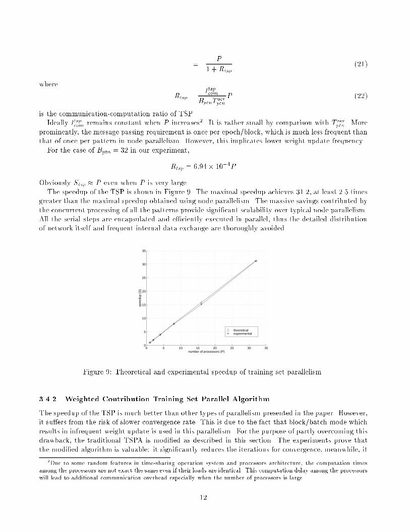
=P
1 +Rtsp(21)
where
Rtsp =ttspcom
BptnTserptn
P (22)
is the communication-computation ratio of TSP.
Ideally ttspcom remains constant when P increases2. It is rather small by comparison with T serptn . More
prominently, the message passing requirement is once per epoch/block, which is much less frequent than
that of once per pattern in node parallelism. However, this implicates lower weight update frequency.
For the case of Bptn = 32 in our experiment,
Rtsp = 6:94� 10�4P
Obviously Stsp � P even when P is very large.
The speedup of the TSP is shown in Figure 9. The maximal speedup achieves 31.2, at least 2.5 times
greater than the maximal speedup obtained using node parallelism. The massive savings contributed by
the concurrent processing of all the patterns provide signi�cant scalability over typical node parallelism.
All the serial steps are encapsulated and e�ciently executed in parallel, thus the detailed distribution
of network itself and frequent internal data exchange are thoroughly avoided.
0 5 10 15 20 25 30 350
5
10
15
20
25
30
35
number of processors (P)
spee
dup
(S)
experimentaltheoretical
Figure 9: Theoretical and experimental speedup of training set parallelism.
3.4.2 Weighted Contribution Training Set Parallel Algorithm
The speedup of the TSP is much better than other types of parallelism presented in the paper. However,
it su�ers from the risk of slower convergence rate. This is due to the fact that block/batch mode which
results in infrequent weight update is used in this parallelism. For the purpose of partly overcoming this
drawback, the traditional TSPA is modi�ed as described in this section. The experiments prove that
the modi�ed algorithm is valuable: it signi�cantly reduces the iterations for convergence, meanwhile, it
2Due to some random features in time-sharing operation system and processors architecture, the computation times
among the processors are not exact the same even if their loads are identical. This computation delay among the processors
will lead to additional communication overhead especially when the number of processors is large.
12

0 5 10 15 20 25 300
2
4
6
8
10
12
14
number of processors (P)
spee
dup
(S)
theoretical experimental
Figure 7: Theoretical and experimental speedup of the algorithm combining the �lter and image region
parallelisms.
update strategy. The block length (number of patterns in each block) should be larger than the number
of available processors to be able to fully utilize all the processor resources.
3.4.1 Implementation of Training Set Parallel Algorithm
Processor 2Processor 1 Processor P
pattern∆
update p, q, t and w
+end loop
∆ = ∆ + pattern∆ ∆
message passing for ∆
end loop∆ = ∆ + pattern= ∆
forcalculate pattern = 1 to L do
∆ pattern
pattern
forcalculate ∆ pattern
pattern
pattern = L+1 to 2L
∆
forcalculate ∆ pattern
pattern
do pattern = Nptn-L+1
update p, q, t and w update p, q, t and w
to Nptn do
end loop
Figure 8: Procedure diagram for training set parallelism. � = f�W;�t;�p;�qg. The number of
patterns in each subset is determined by L = Nptn=P .
The diagram of the training set parallel algorithm (TSPA) is shown in Figure 8. It runs many copies
of the FIC system concurrently by the distribution of the training set across the processors. The training
time for an epoch is given by
Ttspepoch =
Nptn
PT serptn +
Nptn
Bptn
ttspcom (20)
where ttspcom is the communication time for one epoch. It is measured as 2.094ms per epoch.
The speedup of the TSP is
Stsp =T serepoch
Ttspepoch
11

Processor 1
,
Processor Group 1
flt
,
Processor 2
,
Processor P
j z j (A)ij
iz z
∆ z j
end loop
i
∆ zcalculate p(
∆
/M) and p(
zij
j
ji (A) z j
i
calculate p( /M) and p(∆
j
∆ z∆ zz
∆
∆ z
qj
end loop j
for j = 1 to nf do
∆
∆ jp ∆ qj
∆ wi
j ∆ jti
andcalculate
z
and
j = nf+1 to 2*nf do
for j = nf+1 to 2*nf doand∆ jj q j
∆
p
i
∆
jt
and
andcalculate
end loop j
end loop j
for to doi = 1 np for to doi = 1 np for to
calculate p(M/
end loop
to doi = 1 npfor to doi = 1 np∆ w
ij ∆ jt
iandcalculate
for to doi = 1 np
∆ t∆ p ∆ q ∆ wmessage passing for
for
j
and
)
p
p(∆ z/M) p(∆ z/M)
jp qj jt w j
end loop j
jp qj
∆
z
w
j
end loop j
jp qj jt
j
j
end loop j
∆i
message
with otherpassing
groups
do
with otherpassing
groups
∆
i = 1
calculate p(M/ )z∆calculate p(M/
np
)
for
z
j
- (B) ]end loop
/M)∆ z j
i
/M) * p(∆ z j /M)
end loop
calculate = [
/M) and p(∆ z j
/M) * p(∆ z j /M)
∆ zij (A) iz
jizj
∆ z/M) =
j
p(∆ zp(∆ z/M) = p(
p(∆ zcalculate p(
- (B) ]end loop
/M)∆ z j
i
/M) * p(/M) * p(p( ∆ z j /M)p(∆ z ∆ z
p( ∆ z j /M)/M) =
p( /M) =
calculate = [ - (B) ]end loop
/M)∆ z j
i
/M) * p(/M) * p(p( ∆ z j /M)p(∆ z ∆ z
p( ∆ z j /M)/M) =
p( /M) =
calculate = [
calculate
end loop i
calculate
end loop i
calculate
end loop i
t
∆
w
message passing for and
w
for j = Nflt-nf+1 to Nflt
for j = Nflt-nf+1 to Nflt
, ,update andfor j = Nflt-nf+1 to Nflt do
do
do
message
for j = 1 to nf do
, ,update andfor j = 1 to nf do
, ,update andfor j = nf+1 to 2*nf do
Figure 6: Procedure diagram for combined �lter and image region parallelism. Both the �lters and
the image regions are processed in parallel. Only Processor Group 1 is shown in the �gure. Pflt is
the number of processors per group, nf =Nflt
Pflt, and np =
Nptch
P=Pflt. The shadowed areas show how the
computation load is distributed to processors.
Its communication-computation ratio Rflt+reg is
Rflt+reg =P
0:95 + 3:97� 10�3P: (19)
In Equation 17 to 19, P is the total number of processors being used. Pflt is the number of processors
assigned to the computation of the �lters for a given image region. Obviously it is the most e�cient
to run all the �lters in parallel, thus Pflt can be �xed as equivalent to Nflt. The communication time
tflt+regcom is 2.2104ms per pattern. The corresponding theoretical and experimental results are shown in
Figure 7. The speedup achieves 13.3 by using 27 processors simultaneously.
3.4 Training Set Parallel Algorithms for the FIC System
Training set parallelism (TSP) is a coarse computation granularity approach. It exploits parallelism at
higher level of abstraction. By contrast, the node parallelism which requires network decomposition is
termed as low level partitioning scheme. In TSP, the neural network is duplicated on each processor. A
subset of the training set is allocated to each processor. Training by batch/block is required as weight
10

To avoid the slow I/O operation during the training cycle, all the training patterns are stored in
memory since there is su�cient local memory in each processor. Thus downloading time is only needed
initially. That means the downloading time is very short compared to the total training time and is
eliminated in the time analyses.
3.3 Node Parallel Algorithms for the FIC System
There are several ways to partition the FIC system into a set of slices which can be executed in parallel.
In order to balance the computation load among di�erent processors, the network should be decomposed
as even as possible. Three di�erent decompositions can be considered to solve this problem.
Parallelism among di�erent �lters. In the FIC system, the computation involved with each �lter
are exactly the same. Thus one approach of decomposition is to distribute the �lters across the pro-
cessors. A limitation of this approach is that the maximum speedup is restricted by the number of the
�lters used in the FIC system. Although more �lters can be introduced to improve the reliability in the
recall phase and increase the speedup, there will not be a large number of �lters assumed in the FIC
system.
Parallelism among di�erent image regions. Parallelism on smaller computation granularity can
be exploited to obtain a higher degree of parallelism (DOP, which is de�ned as the number of processors
used to execute a parallel program). A simple method is to decompose the image into several regions
with the same size, and distribute them across the processors. The computation load involved with this
image can then be evenly distributed across those processors. An image consists of 36 patches, each
of which has independent computation with the �lter set. An image region should consist of multiple
number of patches in order to avoid frequent internal data exchange. Since the possible number of image
regions is much larger than that of the �lters, more processors can be used concurrently to achieve a
higher speedup in comparison with the �lter parallelism.
Combined parallelism among di�erent �lters and image regions. To further improve the
speedup through the node level parallelism, the computation granularity can be made even smaller by
combining above two decomposition approaches together. In this case, each processor is responsible for
the computation involved in a group of image patches and a speci�ed (or a subset of) �lter(s).
The detailed implementation of combined parallelism among �lters and image regions is discussed
below. The partitioning among di�erent �lters and image regions can be combined together to use
more processors on the target machine. The processors are split into several groups. Each group is
responsible for a set of image patches and within the group di�erent processors correspond to di�erent
�lters. The communication demand is the same as that in image region parallelism. An algorithm
diagram for one such group is shown in Figure 6.
The training time for an epoch and the speedup in this implementation are given by
Tflt+regepoch = Nptn[
NptchNflt
Ptfp +
Nflt
Pflttf + tflt+regcom ] (17)
Sflt+reg =T serepoch
Tflt+regepoch
=P
0:952+ 3:97� 10�2P: (18)
9

Both node parallelism and pipelining approach try to partition the neural network into several pieces,
and assign a piece of network to one or more processors working with whole training set. While the
training set parallelism tries to partition the training set across the processors but encapsulate an entire
copy of neural network.
3.2 Time Analysis of the Sequential Training Algorithm for the FIC system
For the sake of the speedup analysis in the parallel implementations, the response time of the FIC
system sequential training algorithm is discussed �rst.
Figure 5 shows the sequential training procedure when the preprocessed data of one pattern (one
pattern refers to a pair of reference and test images, see Section 2) is submitted. The pattern mode is
used as weight update strategy.
∆ z)calculate p(M/
∆ zij z j
i (A) z ji
calculate p( /M) and p(∆ z j
end loop j
∆ z∆ z
and∆ jp ∆ qj
∆ wi
j ∆ jti
andcalculate
end loop j
jp qj jt w j
end loop j
Calculate filtersoutputs anddecision output.
Calculate finaildecision output.
- (B) ]end loop
/M)∆ z j
i
/M) * p(/M) * p(p( ∆ z j /M)p(∆ z ∆ z
p( ∆ z j /M)/M) =
p( /M) =
calculate = [for toi = 1 Nptch
for j = 1 to Nflt
calculate
end loop i
for j = 1 to Nflt
, ,update andfor j = 1 to Nflt
do
do
tofor i = 1 Nptch do
do
do
Calculateconnection errors.
Update connections.
Figure 5: Sequential procedure diagram for training the FIC system.
The training time for one pattern T serptn consists of several time components corresponding to the
various computation steps in forward and backward passes of the training procedure given by Equa-
tions 2- 14. More than 99% of the components are directly proportional to the number of �lters (denoted
by Nflt) and/or the number of image patches (denoted by Nptch). Thus Tserptn can be written as
T serptn � NfltNptchtfp +Nflttf (15)
where tfp = 0:8305ms is the time constant related to both �lters and image patches, and tf = 1:5286ms
is the time constant related to �lters only. They are measured by running the program on a single
processor of the CM-5.
The sequential training time for one epoch is thus given by
T serepoch = NptnT
serptn (16)
where Nptn is the number of patterns in the training set.
8

3. It has a faster convergence rate since it updates the weights Nptn times more frequently then the
batch mode, where Nptn is the number of patterns in the training set.
On the other hand, the batch mode is well suited to parallelization because weight errors can be
calculated independently. To improve the convergence rate of batch mode, the weights may have to
be updated more frequently than once per epoch. Thus a hybrid update strategy, the block mode, is
adopted in many parallel implementations of neural network.
The parallelism inherent in the multilayer ANN paradigm itself reveals several di�erent types of
parallelism [16,19]:
(b)
(a) (c)
output layer
hidden layer
input layer
Processor 1
Processor 2
Processor PProcessor 1
Processor PProcessor 2Processor 1
Pattern 1 to n Pattern (n+1) to 2n Pattern [(P-1)n+1] to Pn
Figure 4: Three types of parallelism inherent in ANN paradigm: (a) Node parallelism. (b) Training set
parallelism. (c) Pipelining. The dotted lines show how the network is mapped to processors.
.
� Node Parallelism The nodes at the same layer are partitioned and distributed over the pro-
cessors. Each processor concurrently simulates a slice of the network over the whole training set
(Figure 4a). Further, the computation within each node may also run in parallel. In this method,
the weights can be updated by using pattern mode.
� Training Set Parallelism The training set is partitioned into several subsets, while the whole
neural network is duplicated on each processor. Each processor works with a subset of the training
set (Figure 4b). The weights are updated by using the block mode or the batch mode.
� Pipelining The forward and backward passes of di�erent training patterns can be pipelined, i.e.,
while the output layer processor calculates output and error values, the hidden layer processor
concurrently processes the next training pattern (Figure 4c). Pipelining requires a delayed weight
update1 or block/batch mode.
1The delayed weight update mode is a variation of pattern mode which is especially designed for pipelining implemen-
tation. In this mode, weight update is delayed after the presentation of several patterns.
7

3 Parallel Algorithms for the FIC System
The various parallel approaches investigated in the paper are targeted for a coarse grain distributed
memory parallel architecture. A 32-node CM-5 is used as the platform for implementations and mea-
surements.
In order to develop e�cient parallel algorithms for the FIC system, a careful examination of the par-
allelism inherent in the ANNs themselves is fundamental. Three types of parallelism: node parallelism,
training set parallelism (TSP) and pipelining, as well as their combinations are investigated in this
section. The results show that signi�cant speedup can be obtained through the e�cient exploration of
parallelism inherent in the FIC system.
3.1 Parallel Paradigms for ANNs
total average error < tolerance
begin
output layer
hidden layer
input layer
(b)(a)
comparison with desired output
forward propagation of activations
presentation of training patterns
back proopagation of errors
weights update
end
weight initialization
Yes
No
forw
ard
pass
backward pass
Figure 3: (a) A three-layer ANN. (b) Backpropagation training procedure.
A typical backpropagation algorithm for a multilayer ANN is described by Figure 3. An important
feature which a�ects the design of a parallel neural network algorithm is the weight updating strategy.
Basically there are three di�erent strategies described as follows:
� Pattern Mode Strategy Weight updating is performed after the presentation of each training
pattern.
� Batch Mode Strategy Weight updating is performed after the presentation of all the training
patterns that constitute an epoch.
� Block Mode Strategy Weight updating is performed after the presentation of a subset of the
training patterns.
The pattern mode has some advantages over the batch mode [8]:
1. It requires less local storage for the weights.
2. The patterns can be presented to the network in a stochastic manner, which makes some training
algorithms, i.e., the backpropagation, less likely to be trapped in a local minimum.
6

Summarily, the adjustable parameters of the neural network are wjx;y, t
j , pj , and qj . In this imple-
mentation, their total number is (7� 7+ 1)� 3+ 2� 3 = 156. The parameters are initialized randomly
within a small range. They are then iteratively adjusted after the presentation of each image pair, by
gradient descent on the cross entropy error measure H . The equations for calculating parameter errors
are given below.
Assume p = p(M=�z). Let
c =
(�(u=v)� p if P = 1
�(u=v)� p2=(p� 1) if P = 0(9)
cw = 2c ln(1� pj)(1� qj)
pjqj(10)
where
u = p(�z=M)p(M)
v = p(�z=M)p(M):
Then the cross entropy errors of adjustable parameters can be derived from Equations 3- 8:
@H
@pj= c(n=pj �
1
pj(1� pj)
Xi
�zji ) (11)
@H
@qj= c(n=qj �
1
qj(1� qj)
Xi
�zji ) (12)
@H
@wjx;y
= cwXi
f[zji (A)� zji (B)][z
ji (A)(1� z
ji (A))Irs(A)�
zji (B)(1� z
ji (B))Irs(B)]g (13)
@H
@tj= cw
Xi
f[zji (A)� zji (B)][z
ji (A)(1� z
ji (A))� z
ji (B)(1� z
ji (B))]g: (14)
The summation of i is taken from 1 to 36, the total number of patches per image. j = 1; 2; 3 is the
number of �lters used in the FIC system.
By gradient decent method,
pj(k + 1) = pj(k)� �@H
@pj;
qj(k + 1) = qj(k)� �@H
@qj;
wjx;y(k + 1) = wj
x;y(k)� �@H
@wjx;y
;
tj(k + 1) = tj(k)� �@H
@tj
where � � 1 is the learning rate.
After the neural network part of the FIC system is trained by 100 image pairs, a recognition accuracy
of 93:78% is obtained. One approach to further improve the recognition accuracy is to increase the
training set size. However, it will be very time consuming if the network is trained on serial computer
with a large training set. In this case, the parallel implementation becomes mandatory.
5

training. Denote i as the position of (x; y). For the outputs of each �lter j, the squared di�erence
between two images is
�zji (A;B) = [z
ji (A)� z
ji (B)]
2: (2)
Denote �z = �z(A;B) as the array of all �zji (A;B) for all position i and �lter j.
2.2.2 Decision
The purpose of the decision part of the network is to estimate the probability p = p[M(A;B)=�z(A;B)] =
p(M=�z) of a match between images A and B, given the evidence �z provided by the convolution �l-
ters. The decision part can be viewed as a binary Bayesian classi�er. There are four key ingredients to
the decision network:
1. Because the output of the network is to be interpreted as a probability, the usual least mean
square error used in most backpropagation networks does not seem to be an appropriate measure
of network performance. For probability distributions, the cross entropy between the estimated
probability output p and the true probability P , summed over all patterns, is a well-known infor-
mation theoretic measure of discrepancy
H(P; p) =X(A;B)
(P logP
p+ Q log
Q
q) (3)
where, for each image pair, Q = 1� P and q = 1� p.
2. Using Bayes inversion formula and omitting, for simplicity, the dependence on the image pair
(A;B)
p(M=�z) =p(�z=M)p(M)
p(�z=M)p(M) + p(�z=M)p(M)(4)
and choosing appropriate values for p(M) and p(M).
3. Making the simplifying independence assumption that
p(�z=M) =Yi;j
p(�zji=M) (5)
p(�z=M) =Yi;j
p(�zji=M): (6)
In the center of a �ngerprint where there is more variability than in the periphery, it is a reasonable
approximation, which leads to a simple network architecture and, with hindsight, yields excellent
results.
4. Using binomial model for p(�zji=M) and p(�z
ji=M):
p(�zji =M) = p1��zjij (1� pj)
�zji = pj(1� pj
pj)�z
ji (7)
p(�zji=M) = q�zjij (1� qj)
1��zji = (1� qj)(qj
1� qj)�z
ji (8)
with 0:5 � pj ; qj � 1. This is again only an approximation used for its simplicity and for the
fact that the feature di�erences �zji are usually close to 0 or 1. In this implementation and for
economy of parameters, the adjustable parameters pj and qj depend only on the �lter. In a more
general case they could also depend on location.
4

2.2 Neural Network Decision Stage
The decision stage is the neural network part of the algorithm. The network has a pyramidal archi-
tecture, with two aligned and compressed central regions as inputs along with a single output p (see
Figure 2). The bottom level of the pyramid corresponds to a convolution of the compressed central
Z(A) Z(B)
P(M(A,B))
Z
Decision Network
Squared differences of convolution filter outputs
Convolution filter outputs
Convolution filters
Central Region A Central Region B
Figure 2: Neural network architecture [2].
regions with respect to a set of �lters or feature detectors. The decision layer implements results from
a probabilistic Bayesian model for the estimation of p, based on the output of the convolution �lters.
Both the �ltering and decision part of the network are adaptable and trained simultaneously.
2.2.1 Convolution
The two central regions are �rst convolved with a set of adjustable �lters. Three di�erent �lters are
used in our application. Each �lter has a 7�7 receptive �eld and moves across all the image by 5 pixels
each step.The two neighboring receptive �elds have an overlap of 2 pixels to approximate a continuous
convolution operation. Thus each 32 � 32 compressed central region is transformed into three 6 � 6
output arrays, one for each �lter. The output of �lter j at position (x; y) in one of these arrays is given
by (for instance for A):
zjx;y(A) = f(X
wjx�r;y�sIr;s(A) + tjr;s) (1)
where Ir;s(A) is the pixel value in the compressed central region of image A at the position of (r; s), f
is the sigmod function
f(x) =1
1 + e�x;
wx�r;y�s is the weight of synaptic connection from the position of (r; s) in the compressed central region
to the position of (x; y) in the array of �lter outputs, and tj is a threshold. The summation in Equation 1
is taken over the 7� 7 patch coincident with the receptive �eld of the �lter at the (x; y) location. The
threshold and the weights of 7� 7 receptive �eld are characteristic of the �lter, so that they can also be
viewed as the parameters of a translation invariant convolution kernel. They are shared within an image
but also across the images A and B. These 7 � 7 + 1 = 50 parameters are adjustable during network
3

obtained by these implementations proves that highly general purpose parallel computers can compete
with the performance of special purpose computers while avoiding dedicated hardware elements with
dedicated connection paths.
In 1994, we developed a neural network based automated Fingerprint Image Comparison (FIC) system
[22]. The purpose of the development is to meet the rapidly growing load of �ngerprint recognition in
FBI Identi�cation Division. When presented with a pair of �ngerprint images, the FIC system outputs
an estimate of the probability that the two images originate from the same �nger. The preliminary test
showed 93:78% recognition accuracy after the system was trained by 100 pairs of images.
The FIC system was �rst implemented on SUN Sparc workstation. The training time for 100 pairs
of images was about 6 to 8 days. Such a long time made it di�cult to extend the training set for higher
recognition accuracy.
The goal of this paper is to develop e�cient parallel algorithms by exploiting parallelism inherent in
the FIC system. In order to do this, node parallelism, training set parallelism (TSP), and combined
parallelism are examined. Theoretical analyses of the performance of various parallel algorithms are
performed. To obtain better speedup performance and to overcome the drawback of TSP, several new
extensions are investigated.
The paper is organized into four sections. Section 2 describes a neural network based FIC system
architecture. Section 3 presents a variety of parallel algorithms for the FIC system. The performances
of these algorithms are compared based on the theoretical analyses and the experimental results of the
implementations. Section 4 summarizes the main conclusions of this paper.
2 The FIC System Architecture
The neural network based Fingerprint Image Comparison (FIC) system presented in this section is
mainly based on an algorithm described by Baldi and Chauvin in [2] and modi�ed in [22]. The system
consists of two components: a preprocessor and a neural network based decision stage (Figure 1). When
presented with a pair of �ngerprint images, the system outputs an estimate of the probability that the
two images originate from the same �nger. The �ngerprints are obtained from the NIST (National
Institute of Standards and Technology) Fingerprint Database CD-ROM which contains 4000 (2000
pairs, two di�erent rollings of the same �nger) 8-bit grey scale images of randomly selected �ngerprints.
Each print is 512� 512 pixels with 32 rows of white space at the bottom of the print.
NEURAL NETWORK
DECISIONPREPROCESSORtwo grey scale
fingerprint imagestwo compressed central regions
probabilityof matching
Figure 1: Operations of the FIC system.
2.1 Preprocessing Stage
The purpose of the preprocessing stage is to extract a central region from each one of the two input
images, and to align the two central regions. The outputs of the preprocessor are two compressed central
regions with 32� 32 pixels each. The detailed algorithm of preprocessor is described in [22].
2
Parallel Algorithms for an Automated Fingerprint
Image Comparison System
Hany H. Ammar and Zhouhui Miao
Department of Electrical and Computer Engineering
West Virginia University, Morgantown, WV 26506, USA
October 6, 1995
Abstract
This paper addresses the problem of developing e�cient parallel algorithms for the training proce-
dure of a neural network based Fingerprint Image Comparison (FIC) system. The target architecture
is assumed to be a coarse-grain distributed memory parallel architecture. Two types of parallelism:
node parallelism and training set parallelism (TSP) are investigated. Theoretical analysis and exper-
imental results show that node parallelism has low speedup and poor scalability, while TSP proves
to have the best speedup performance. TSP, however, is amenable to a slow convergence rate. In
order to reduce this e�ect, a modi�ed training set parallel algorithm using weighted contributions
of synaptic connections is proposed. Experimental results show that this algorithm provides a fast
convergence rate, while keeping the best speedup performance obtained.
The combination of TSP with node parallelism is also investigated. A good performance is
achieved by this combiation approach. This provides better scalability with the tradeo� of a slight
decrease in speedup.
The above algorithms are implemented on a 32-node CM-5.
1 Introduction
A large scale arti�cial neural network (ANN) used to solve the real-world application problems, such
as pattern recognition, vision and speech recognition, can require enormous amounts of computational
resources. The mass of processing elements and synaptic connections that comprise an ANN, as well
as a generally required large training set, make ANN inherently computation intensive. In fact, most
of the serial computers available today are bound to be overwhelmed by the computational demands of
ANNs for real-world application [16].
Generally, the target machines for implementing parallel neural network simulations fall into two
categories: special-purpose parallel processors and general-purpose parallel computers. For the special-
purpose parallel processors, they have the advantages of very high processing speed, low cost and small
size, whereas it loses the exibility once a neural network has been \cast" on it.
On the other hand, general-purpose parallel computers can be applied to a wide variety of neural net-
work models. In these applications, the parallel models are created in software while some compromise
is provided between the exibility and the speedup.
Some widely used training algorithms for multilayer neural networks, especially the backpropagation
algorithm, have been implemented on several types of supercomputers, such as the Warp [14], the
Connection Machine [15, 16, 23], the IBM GF 11 [20], and the Fujitsu AP1000 [19]. The speedup
1

Contents
1 Introduction 1
2 The FIC System Architecture 2
2.1 Preprocessing Stage : : : : : : : : : : : : : : : : : : : : : : : : : : : : : : : : : : : : : : 2
2.2 Neural Network Decision Stage : : : : : : : : : : : : : : : : : : : : : : : : : : : : : : : : 3
2.2.1 Convolution : : : : : : : : : : : : : : : : : : : : : : : : : : : : : : : : : : : : : : : 3
2.2.2 Decision : : : : : : : : : : : : : : : : : : : : : : : : : : : : : : : : : : : : : : : : : 4
3 Parallel Algorithms for the FIC System 6
3.1 Parallel Paradigms for ANNs : : : : : : : : : : : : : : : : : : : : : : : : : : : : : : : : : 6
3.2 Time Analysis of the Sequential Training Algorithm for the FIC system : : : : : : : : : 8
3.3 Node Parallel Algorithms for the FIC System : : : : : : : : : : : : : : : : : : : : : : : : 9
3.4 Training Set Parallel Algorithms for the FIC System : : : : : : : : : : : : : : : : : : : : 10
3.4.1 Implementation of Training Set Parallel Algorithm : : : : : : : : : : : : : : : : : 11
3.4.2 Weighted Contribution Training Set Parallel Algorithm : : : : : : : : : : : : : : 12
3.5 Combined Parallel Algorithms : : : : : : : : : : : : : : : : : : : : : : : : : : : : : : : : : 14
3.6 Comparing the Performance of Parallel Implementations : : : : : : : : : : : : : : : : : : 15
4 Conclusions 18
i