Powertrain dynamic torque reduction using clutch slip control

ANDREAS SZILASSY

MARCUS ENGMAN

Master of Science Thesis

Stockholm, Sweden 2014

Powertrain dynamic torque reduction using clutch slip control

Andreas Szilassy

Marcus Engman

Master of Science Thesis MMK 2014:49 MDA 482

KTH Industrial Engineering and Management

Machine Design

KTH Vehicle Dynamics

SE-100 44 STOCKHOLM

i

Master of Science Thesis MMK 2014:49 MDA 482

Powertrain dynamic torque reduction using clutch slip control

Andreas Szilassy

Approved

2014-06-25

Examiner

Jan Wikander

Supervisor

Mikael Hellgren

Commissioner

Scania CV

Contact person

Erik Gustafsson

Abstract The torque dynamic caused by the firing pulse from diesel engines set high robustness

demands for gearboxes and final drives in today’s heavy duty trucks. If these dynamic loads

could be eliminated or dampened, the driveline can be built lighter because of the lower

demands which in turn would save fuel for the driver and material cost for the manufacturer.

There exist solutions to this problem that include expensive and complicated hardware; for

example the double mass flywheel, but there is one opportunity that is potentially for free to

the manufacturer, namely clutch slip control.

The hypothesis of this thesis is that the torque oscillations from the engine can be reduced by

controlling the clutch slip velocity. It is also evaluated if it is possible to control a slip using

existing hardware in a Scania powertrain and if the control performance can be improved by

changing one of the powertrain parameters. For the scope of this thesis, the wear rate and

temperature of the clutch when slipping is not considered.

The first step of the thesis is to construct a MBS model of the powertrain in question. Further

on, two control designs, namely fuzzy control and two degrees of freedom control are

implemented using model based control design. Both control algorithms are implemented in a

heavy duty truck and the performance is evaluated. To find the parameter that constrains the

performance, a parameter variation is performed using the developed model to save both time

and cost.

It is proved that the torque dynamics from the diesel engine can be dampened by forty to

eighty percent in amplitude by slipping the clutch and that the implemented control design

gives acceptable results for gears seven to twelve using existing hardware. The parameter

variation shows that the actuation delay is the main limiting factor, enabling stable control at

the first gear if removed completely.

The slip control concept shows potential but sets high demands for hardware specification,

especially for actuation delays if all gears are to be used with slip control. Using existing

hardware, the control is fully implementable for gears seven to twelve with good results.

ii

iii

Examensarbete MMK 2014:49 MDA 482

Kopplingsslirreglering för minskat dynamiskt moment i drivlinan

Andreas Szilassy

Godkänt

2014-06-25

Examinator

Jan Wikander

Handledare

Mikael Hellgren

Uppdragsgivare

Scania CV

Kontaktperson

Erik Gustafsson

Sammanfattning

Det dynamiska momentet som tändpulserna ger upphov till i dieselmotorer ställer höga krav

på robusthet och hållfasthet hos växellådor och slutväxlar i lastbilar. Om dynamiken kunde

elimineras eller dämpas ut vore det möjligt att bygga transmissionen lättare eftersom kraven

på robusthet och hållfasthet skulle minska. Detta skulle i slutändan betyda lägre

bränsleförbrukning för åkeriet och lägre materialkostnader för lastbilstillverkaren. I dagsläget

finns det flera dyra lösningar som bygger på komplicerade mekaniska koncept, däribland

dubbelmassesvänghjulet, men det finns en möjlighet som potentiellt är gratis för tillverkaren

ur ett materialperspektiv, nämligen kopplingsslirkontroll.

Hypotesen i det här examensarbetet är att momentoscillationerna från motorn kan reduceras

genom att kontrollera slirhastigheten i kopplingen. Det utvärderas också om det är möjligt att

kontrollera slirhastigheten genom att använda komponenterna i en befintlig, produktionssatt

Scania drivlina och om det finns en nyckelparameter i hårdvaran som tydligt begränsar

regleringens prestanda. Kopplingens temperatur och slitning anses vara utanför ramen för

detta examensarbete och behandlas inte i denna rapport.

Som första steg i utvecklingen konstrueras en MBS-modell av drivlinan i fråga.

Fortsättningsvis implementeras två reglerstrukturer, nämligen fuzzy-reglering och

tvåfrihetsgradsreglering genom att använda modellbaserad utveckling. För att utreda

prestandan i dagens system implementeras båda reglerstrukturerna i en lastbil där verklig

provning utförs. För att hitta den begränsande faktorn utförs en parametervariation i den

utvecklade modellen istället för i en lastbil, vilket sparar både tid och minskar kostnaden.

I det här examensarbetet har det visats att momentdynamiken från dieselmotorn kan dämpas

ut med fyrtio till åttio procent i amplitud genom att slira på kopplingen och att den

implementerade reglering ger en acceptabel prestanda för växlarna sju till tolv i existerande

hårdvara. Den utförda parametervariationen visar att fördröjningen mellan beräknad styrsignal

och faktisk aktuering är mest begränsande och att en eliminering av denna möjliggör stabil

reglering på första växeln.

iv

Kopplingsslirregleringskonceptet visar stor potential men sätter höga krav på hårdvara; inte

minst aktueringsfördröjningen om regleringen ska användas på alla växlar. Med existerande

drivlina är dock regleringen fullt implementerbar sju till och med tolv..

v

FOREWORD

The work of this master thesis was conducted at the department for Powertrain Control

Systems at Scania CV AB in Södertälje with support and supervision from the department of

Engineering Design, track Mechatronics and the department of Aeronautical and Vehicle

Engineering, division of Vehicle Dynamics at the Royal Institute of Technology (KTH) in

Stockholm.

Due to the different areas of expertise of the authors, some parts of the development process

have been individually developed by a single author while some are joint efforts. When

developing the feedback loop; Engman focused at a fuzzy logic knowledge based feedback

controller while Szilassy focused on a pole placement designed feedback loop using the

Diophantine equation.

We would like to take the opportunity to thank our supervisors; Erik Gustafsson at Scania for

providing guidance and help throughout the development, Fredrik Jarngren for help with

testing, Lars Drugge at KTH Vehicle Dynamics and Mikael Hellgren at KTH Mechatronics

for support and motivating comments on our progress. Special thanks to NEC for making this

master thesis possible and for interesting discussions during lunch breaks.

Andreas Szilassy

Marcus Engman

Södertälje, 5/6-14

vi

vii

NOMENCLATURE

The nomenclature contains all notations and abbreviations used throughout this thesis listed

in the order of appearance. All notations are complete with description and unit of measure if

applicable.

Notations

Symbol Description Unit

Combined engine, flywheel and clutch cover inertia

Clutch disc inertia

Gearbox inertia

Propeller shaft inertia; first half

Propeller shaft inertia; second half

Drive shaft inertia; first half, differential inertia

Drive shaft inertia; second half, wheel and vehicle

inertia

Clutch disc spring stiffness ⁄

Clutch disc damping ⁄

Propeller shaft stiffness ⁄

Propeller shaft damping ⁄

Drive shaft stiffness ⁄

Drive shaft damping ⁄

Gearbox gear ratio

Final drive gear ratio

Angular velocity for inertia ⁄

Angular position for inertia

Clutch disc hard stop angular position, positive

Clutch disc hard stop angular position, negative

Clutch disc hard stop stiffness ⁄

Torque corresponding to stiffness

Torque corresponding to damping

Torque transferred by the clutch

Summation of external torques on the vehicle

viii

Average torque output from engine

Dynamic torque addition to engine torque from firing

pulses

Resulting torque outputted by the engine

Dynamic torque amplitude gain

Electronic clutch actuator position

Clutch contact point expressed in actuator position

Clutch torque transfer polynomial coefficient 1 ⁄

Clutch torque transfer polynomial coefficient 2 ⁄

Clutch torque transfer polynomial coefficient 3 ⁄

Clutch slip angular velocity ⁄

Clutch slip angular velocity tolerance used in the state

machine ⁄

Clutch slip angular acceleration tolerance ⁄

The maximum torque that can be inputted to the clutch

without causing slip

The torque transferred while slipping

State space representation, state-matrix

State space representation, input-matrix

State space representation, output matrix

State space representation, input-to-output matrix

State space representation, state vector

State space representation, input vector

Jacobian of the state-matrix

Jacobian of the input-matrix

Total gearbox gear ratio

Split gear ratio

Main gearbox gear ratio

Range gear ratio

Firing order frequency

Tractive force of vehicle

ix

Force due to rolling resistance

Force due to air drag

Vehicle mass

Gravitational acceleration ⁄

Road grade

Drag coefficient of vehicle

Density of air ⁄

The inertia of the crankshaft

The inertia of the piston of the connecting rod

The inertia of the damper in the engine

The inertia of the crank shaft front end

The inertia of the flywheel

The inertia of the clutch cover

The inertia of the engine fan

Clutch disc inner radius

Clutch disc outer radius

Number of friction surfaces in the clutch

Clutch velocity tolerance ⁄

Wheel rolling radius

Rolling resistance coefficient

Vehicle frontal area

The power loss in the clutch

σ Scania internal information

x

xi

ABBREVIATIONS

ECA Electronic Clutch Actuator

MBS Multi Body System

EP-model Elasto-plastic model

FKBC Fuzzy Knowledge Based Controller

LQG Linear Quadratic Gaussian

LTR Loop Transfer Recovery

LQ Linear Quadratic

CAN Controller Area Network

AMT Automated Manual Transmission

PPBC Pole Placed Based Controller

ECU Electronic Control Unit

SISO Single Input Single Output

CARIMA Controller Auto-Regressive Integrated Moving-Average

IMC Internal Model Control

SIMC Simple Internal Model Control

PID Proportional Integrating Derivative

ARX Derivation of ARMAX, Autoregressive–Moving-Average Model

xii

xiii

TABLE OF CONTENTS

1 INTRODUCTION ....................................................................................................................................... 1

1.1 Background ............................................................................................................................................... 1

1.2 Problem description .................................................................................................................................. 1

1.3 Project purpose ......................................................................................................................................... 2

1.4 Delimitations............................................................................................................................................. 2

1.5 Method ...................................................................................................................................................... 3

1.6 System introduction................................................................................................................................... 4

2 FRAME OF REFERENCE ........................................................................................................................ 9

2.1 Automotive powertrain modelling ............................................................................................................. 9

2.2 Controller concept .................................................................................................................................. 17

2.3 Fuzzy feedback control theory ................................................................................................................ 19

3 MODELING .............................................................................................................................................. 25

3.1 Analytic Powertrain model ..................................................................................................................... 25

3.2 A linear model for control ...................................................................................................................... 29

3.4 Simulation Model .................................................................................................................................... 34

4 CONTROL DESIGN ................................................................................................................................. 43

4.1 Clutch control system architecture ......................................................................................................... 43

4.2 Feed forward .......................................................................................................................................... 44

4.3 Output normalization .............................................................................................................................. 44

4.4 Trajectory control ................................................................................................................................... 45

4.5 Predictor ................................................................................................................................................. 45

4.6 Fuzzy feedback control ........................................................................................................................... 46

4.7 Pole placement feedback controller design ............................................................................................ 49

4.8 Filter design ............................................................................................................................................ 62

4.9 Engine PI-controller ............................................................................................................................... 63

4.10 Powertrain parameter variation ........................................................................................................ 63

4.11 Implementation .................................................................................................................................. 64

5 RESULTS ................................................................................................................................................... 65

5.1 Model results .......................................................................................................................................... 65

5.2 Simulated controller results .................................................................................................................... 78

5.3 Robustness of the controllers .................................................................................................................. 84

5.4 Measured control results ........................................................................................................................ 86

5.5 Powertrain parameter variation ............................................................................................................. 98

5.6 Torque dynamics comparison ............................................................................................................... 103

6 DISCUSSION AND CONCLUSIONS ................................................................................................... 105

xiv

6.1 Discussion ............................................................................................................................................. 105

6.2 Future work .......................................................................................................................................... 110

6.3 Conclusions........................................................................................................................................... 111

7 BIBLIOGRAPHY ................................................................................................................................... 113

APPENDIX A: LINEARIZED STATE SPACE REPRESENTATION .............................................................

APPENDIX B: LINEAR STATE SPACE REPRESENTATION .......................................................................

APPENDIX C: SIMULATION MODEL ..............................................................................................................

APPENDIX D: SIMPLIFIED STATE SPACE REPRESENTATION ..............................................................

1

1 INTRODUCTION

The introduction describes the problem and its background together with what methods that

are suitable for finding a solution to the issue. A short introduction to the system is also given

to introduce the reader into the world of powertrain control.

1.1 Background

Cost is a very important factor for truck manufacturers. Every little bit that can help reduce

the cost, for the manufacturer or their customers, in one way or another is of great importance.

For a manufacturer to be competitive the product range must be appealing, affordable and

offer great value. One way of improving these properties is by continuous improvements

without raising costs more than necessary. In other words, there is a challenge to solve

existing problems by using approaches that require less expensive parts or even better

approaches that uses existing parts.

The electronic control units of today’s trucks give a lot of opportunities to control the

hardware in smart ways to improve the performance without upgrading the hardware, which

often is quite expensive. Computers can also be used in conjunction with altered hardware to

enable new functions of a trucks driveline. In a Scania truck for example, there are numerous

electronic control units (ECUs) performing different tasks and interacting with each other,

improving the vehicle performance.

Due to the high grade of existing communication between the control units that interface with

the different actuators and sensors, it is possible to apply new ways to control the actuators

and use the different sensors without the need to establish new connections.

1.2 Problem description

Due to the various torsional flexibilities in the driveline and the dynamical changes in the

torque being transferred from the engine, the driveline is wound up by the torque supplied and

will start to oscillate when torque transients appear[1]. When the driveline starts to oscillate,

the oscillations are transferred to the rest of the truck which could cause an uncomfortable

movement for the driver and excite frame modes which may create noise. Oscillations with

large torque amplitude does also lead to high demands regarding the robustness of the

driveline, which in turn leads to a heavier and more bulky driveline.

1.2.1 Alternative solutions

The oscillations in the driveline have so forth been reduced by the use of a single mass

flywheel, which is adding a large inertia to the system [2]. A more effective way to reduce the

impact of the oscillations is to add a double mass flywheel, which can be explained by the tire

model in Figure 5. The engine is attached to the inner mass while the rest of the driveline is

attached to the outer, giving the system an extra spring and damper pair. The double mass

flywheel will reduce oscillations to a greater extent than a single mass flywheel if set up

correctly. This could however cause even higher torque fluctuation on the engine side of the

clutch for the eigenfrequencies of the flywheel which could lead to problems for the different

components in the engine. Adding a dual mass flywheel also leads to a larger vehicle mass

which increases the fuel consumption of the truck.

Another solution to reduce the oscillations is to extend the oscillating reducing systems that

already exist today. There exist torsion springs and dampers in the clutch whose purpose is to

2

dampen the oscillations and these could possibly be increased to dampen the oscillations even

more. However this would probably add an extra cost to the vehicle and could increase the

energy losses in the driveline.

One, quite drastic solution to eliminate the driveline oscillations would be to change the

engine from a diesel engine to an electrical motor which would be able to deliver a torque

with less unwanted dynamics. This approach is halted by the fact that the electrical systems

that exist today are too heavy and uses too much space to be a serious alternative for long

haulage. The battery pack would have to be enormous for an electric motor to be able to

power the truck alone for larger distances. Moreover, the cost to implement a fully electric

driveline that could meet the requirements would probably be large. To reduce the problem of

the large battery packs needed, there are also experiments with electrifying parts of the road

network to enable electric drive. This, however, only reduces torque dynamics on roads that

are electrified.

Another alternative to reduce the driveline oscillations is to replace the dry friction clutch

with a viscous clutch, like the torque converters used in trucks with automatic hydraulic

transmissions. The benefits of using an automated manual clutch would then be lost and the

energy losses in the clutch would be increased.

There are also some examples of control of the clutch slip in passenger cars with the purpose

of dampening the driveline oscillations [2]. The idea being that when slipping, the torque

transferred can be held more or less constant due to the characteristics of the dynamical

friction. This could be used to filter the torque fluctuations from the engine caused by the

ignition pulses. If a clutch slip could be controlled, the flywheel inertia could be reduced and

the need for a double mass flywheel would disappear. The largest issue with all of the

hardware solutions above is that they come with a cost. Doing changes in the software, such

as implementing a slip controller, is free from a manufacturing point of view and this is what

gives it its appeal. To be able to control a clutch slip a certain level of precision and speed is

needed for the actuators and sensors, which is depending on what demands are set on the

controller performance.

1.3 Project purpose

The purpose of this study is to evaluate the possibility of controlling a clutch slip with the

current driveline sensors and actuators in a Scania vehicle and evaluate which sensors and

actuators that prevent further improvements regarding slip control. The improvements should

be analyzed for different slip speed regions (e.g. the stick-slip region) and engine torques. The

purpose of the clutch slip speed controller is to reduce the dynamical changes in the torque

being transferred from the engine to the rest of the powertrain. The slip will be controlled by

primarily controlling the position actuated by the ECA, Electronic Clutch Actuator.

In addition to the system evaluation, the hypothesis being tested in this thesis is that the torque

oscillations from the engine can be reduced by controlling the clutch slip velocity.

1.4 Delimitations

When slipping, there will be energy losses in the clutch. The energy losses will lead to a

higher clutch temperature, which may damage the components of the clutch. The wear and

possible damage will not be assessed or analyzed during this project but will be taken into

consideration, due to safety aspects, when the implemented controller is tested in a heavy duty

truck. The heightened temperature will also lead to thermal expansion, contact point change

and slightly different friction characteristic in the clutch. The problems that may arise due to

3

this will not be dealt with directly but will be taken into consideration when designing the

controller.

1.5 Method

In a product development process it is always valuable to identify the best method for the

current project. The different product development methods that have been identified as

relevant to this project are briefly discussed below. There is a need to develop a system which

the controller could be evaluated upon.

1.5.1 Rapid Prototyping

To rapid prototype a model of the system could be seen as an approach to our problem.

However it is not possible to prototype an entire driveline with all the relevant dynamics and

functions in time and with a reasonable cost.

1.5.2 Model Based Development (MBD)

To construct a model and use it for testing the performance of different control concepts and

tuning of the different controllers is a useful approach for this kind of project since it reduces

the test time when comparing to in vehicle tests. The following three methods are of interest

for this project and require parts of a model or a full model to work.

Software in the loop (SIL), when the generated code modules interacts with each other and

possibly with the plant model could be an interesting approach to verify the code generation

process from Simulink to C and detect possible input/output problems.

Processor in the loop is of significance since the system that are studied consists of different

processors communicating with each other with a critical communication delay caused by the

bit rate in the CAN bus. However, it requires a lot of time to set it up properly since the real

system is quite complex with a lot of different processors and sensors communicating with

each other. The PIL approach will probably not be time effective since we have a complete

system available.

Hardware in the loop could be interesting if it was possible to setup a driveline, or parts of the

driveline (e.g. only the clutch), without the rest of the vehicle to enable a quicker testing. This

approach would be quite expensive and allocate a lot of test equipment. If this should be

implemented, the benefits with this setup contra a full vehicle setup would had to be analyzed

properly to motivate it from an economic perspective.

1.5.3 Vehicle testing

To test the developed code directly in a vehicle is another option, which would mean that the

controller always will be evaluated and tuned with the actual system limitations of the system

present. With this approach, the testing will not be able to be performed automatically and it

will be difficult to change the performance of the different components in the driveline to

evaluate the effects. If the testing shall be performed in a vehicle a dependency of external

personal is introduced since neither of the project participants have the necessary driver’s

license.

4

1.5.4 Methods chosen

MBD with SIL is the method chosen since the time consumption and cost for HIL and PIL

would be too large and it would be too difficult to test the possible HW improvements in a

full vehicle. A model reduces the time for testing the controller and enables parameter

variation without involving new hardware or software.

SIL allows the testing of possible input/output problems without being too time consuming,

which reduces the risk of having bugs that easily could be fixed in the beginning of the

development but that could cause a lot of problem later on in the development process.

At the end of the development process the developed controller will be tested in a vehicle to

validate results from the model and to tune the control further to account for modeling errors

or simplifications.

1.6 System introduction

The system to be controlled consists of a typical Scania truck. The particular vehicle chosen

for this project is a test vehicle named Fronda. Fronda, displayed in Figure 1, uses one of the

most common configurations that Scania has to offer, namely a 6x2 chassis designed to carry

standard containers. The 6x2 abbreviation simply translates to a vehicle with three axles (six

wheels) and one driven axle (two wheels). By convention, the driven axle is the second one.

Figure 1: The modelled vehicle Fronda.

Scania offers a range of different engines and gearboxes designed for different customer

requirements and scenarios. The test vehicle is equipped with a front in-line mount 13 liter

DC13 engine with six in-line cylinders. The engine is connected to a Scania GRSO905R

gearbox with Opticruise (Scania's automated gear shift control system), via a dry friction

clutch. The output shaft of the gearbox is connected to a P780 final drive via a propeller shaft.

Finally, the wheels are connected to the final drive with drive shafts.

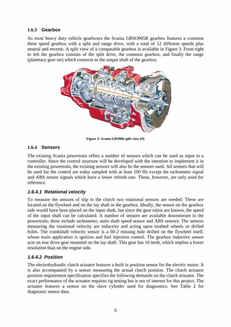
1.6.1 Clutch and flywheel

The clutch used for the tests is a common dry friction clutch with two wear surfaces; one on

each side of the clutch driven plate. The driven plate is equipped with dual spring setups to

reduce fluctuations in torque from the diesel engine. The flywheel connected to the engine

output shaft acts as a mounting point for the clutch cover, these two parts creates the other

side of the two friction surfaces used in the clutch. A split view of a clutch cover and pressure

5

plate is available to the far right of Figure 3. The flywheel is a simple single mass flywheel,

which means that there are no dampers or springs present in the flywheel itself. In Figure 3,

the flywheel would be mounted axial and to the right of the driven plate.

1.6.2 Clutch actuator

The Scania Opticruise gearbox control system features an electro-hydraulic clutch actuator

schematically pictured in Figure 2.

Figure 2: Electronic clutch actuator schematic, the blue sections are hydraulic.

A permanent magnet synchronous motor coupled to a mechanical linear ball screw actuator

acts as the driver input. The ball screw is attached to a hydraulic piston acting as the master

cylinder in a common clutch system. The hydraulic fluid (marked blue) is pushed by the

master cylinder that pushes a slave cylinder; this cylinder is in turn connected to the nonlinear

clutch cover diaphragm spring via a mechanical linkage. The main concept is to apply

different reference positions to the electric motor and thereby varying the normal force on the

pressure plate to determine the amount of torque that can be transferred through the clutch.

The ECA position is internally controlled by a position controller. The actuator data is

available in Table 1.

Table 1: Clutch actuator specified performance for normal operating mode.

Property Value

Release stroke time @ 24-32V σ

Max overshoot for step response σ degrees in motor position

Max error after 100 ms from 120 deg

from target

σ degrees

It is worth noting that if the operating temperature is outside of the specified range the

performance is heavily degraded. Since the specifications listed are from a requirement

specification the real actuator may show better performance. The properties above can be

considered as a worst case scenario. According to the specifications the precision of the

position control in the ECA is high.

The actuator also features two modes, in the specification labeled as “Normal Performance”

and “Reduced Performance” which is set by the governing gearbox managing system. In

“Reduced” the actuator performance is heavily degraded both in accuracy and speed. It is

therefore of vital importance that the actuator is set to “Normal” to utilize the full capacity of

the actuator [3].

Ball screw

Master cylinder

Slave cylinder

Release mechanis

m

Electric motor

6

1.6.3 Gearbox

As most heavy duty vehicle gearboxes the Scania GRSO905R gearbox features a common

three speed gearbox with a split and range drive, with a total of 12 different speeds plus

neutral and reverse. A split view of a comparable gearbox is available in Figure 3. From right

to left the gearbox consists of the split drive, the common gearbox, and finally the range

(planetary gear set) which connects to the output shaft of the gearbox.

Figure 3: Scania GRS900 split view [4].

1.6.4 Sensors

The existing Scania powertrain offers a number of sensors which can be used as input to a

controller. Since the control structure will be developed with the intention to implement it in

the existing powertrain, the existing sensors will also be the sensors used. All sensors that will

be used for the control are today sampled with at least 100 Hz except the tachometer signal

and ABS sensor signals which have a lower refresh rate. These, however, are only used for

reference.

1.6.4.1 Rotational velocity

To measure the amount of slip in the clutch two rotational sensors are needed. These are

located on the flywheel and on the lay shaft in the gearbox. Ideally, the sensor on the gearbox

side would have been placed on the input shaft, but since the gear ratios are known, the speed

of the input shaft can be calculated. A number of sensors are available downstream in the

powertrain; these include tachometer, main shaft speed sensor and ABS sensors. The sensors

measuring the rotational velocity are inductive and acting upon toothed wheels or drilled

holes. The crankshaft velocity sensor is a 60-2 missing hole drilled on the flywheel itself,

whose main application is ignition and fuel injection control. The gearbox inductive sensor

acts on rear drive gear mounted on the lay shaft. This gear has 16 teeth, which implies a lower

resolution than on the engine side.

1.6.4.2 Position

The electrohydraulic clutch actuator features a built in position sensor for the electric motor. It

is also accompanied by a sensor measuring the actual clutch position. The clutch actuator

position requirement specification specifies the following demands on the clutch actuator. The

exact performance of the actuator requires rig testing but is not of interest for this project. The

actuator features a sensor on the slave cylinder used for diagnostics. See Table 2 for

diagnostic sensor data.

7

Table 2: ECA position sensor properties

Property Value

Accuracy ± σ mm

Refresh rate 100 Hz

Communication CAN 250 kbit/s

Measurement range 0 – 90 mm

The ECA also measures the rotational position of the electric motor creating the master

cylinder movement. This sensor is normally used for control and the properties of this sensor

are available in Table 3.

Table 3: ECA motor position sensor data.

Property Value

Accuracy < σ degree

Refresh rate 100 Hz

Communication CAN 250 kbit/s

Measurement range 0 – 6306 degrees

The higher resolution available from the motor position makes it much more suitable for

control applications than the linear position sensor in Table 2 [3].

1.6.4.3 Torque sensors

The test vehicle Fronda is equipped with an extra in-line sensor for measuring both static and

dynamic torque on the input shaft of the gearbox. This setup is proven superior to reaction

type sensors because of the possible error of measuring torque components that are not

present on the shaft itself. A common drawback with in-line torque sensors, besides the cost,

is the need to transfer power and signals to the shaft itself to be able to measure torque. This

can be done in a few different ways; most common are slip rings, rotary transformers or

infrared signals [5].

The sensor used, an ABB Torductor utilizes magnetic fields, much like a rotary transformer. It

is not connected to the vehicle control network and is only for measuring purposes. The

Torductor displays measuring capabilities that are more than adequate for measuring, for

example, the influence of ignition pulses from the engine on the input shaft of the gearbox.

The performance of the Torductor is available in Table 4 [6] .

8

Table 4: ABB Torductor torque transducer data.

Property Value

Resolution 1 Nm or less

Data rate 2.52 kS/s

Communication CAN 250 kbit/s

Measurement range -1500 – +5000 Nm

Since the sensor is disconnected from the rest of the vehicle network it uses its own CAN bus

to communicate with the logging software, this is what enables the high sample rate even

though it uses CAN [7].

To accompany the input shaft torque there is a virtual torque measurement signal available

from the engine management system. The torque signal is created using the amount of

injected fuel which is passed through a transfer function calculating the engine instantaneous

torque output. This signal takes the internal losses of the engine into account. The losses

include; friction, pump losses, etc. Since the signal is tested against actual engine torque

output it is deemed reliable enough.

1.6.4.4 Clutch slave cylinder pressure sensor

The clutch clamping force is of great importance when monitoring the behavior of the clutch.

This force directly controls how much torque that can be transferred through the clutch. Since

this force is difficult to measure directly a pressure sensor is mounted in the slave cylinder of

the clutch actuator unit. This enables the actuator motor position, which is the independent

variable, to be mapped against a force pushing the clutch linkage, which in turn can be

mapped into clamping force. The data for the Keller PA-33X pressure sensor used for this

application is available in Table 5.

Table 5: Slave cylinder pressure sensor.

Property Value

Accuracy 0.1 % (analogue, 3-wire interface)

Refresh rate 500 Hz

Communication CAN via IPEtronik MSENSE

Measurement range 0-100 bar

The pressure sensor is not part of the original system but is connected to the same logging

software as the rest of the system.

1.6.5 Communication

The different ECUs communicate with each other via CAN (Controller Area Network) which

has a limited speed and bandwidth. The ECU that the slip controller will be implemented

upon communicates via CAN to the engine velocity sensors, engine and ECA and directly via

an analogue input to the input shaft velocity sensor. This will cause some delays in the control

loop which will have to be taken into consideration.

9

2 FRAME OF REFERENCE

The frame of reference presents different methods to model components of an automotive

driveline as well as control concepts and theory that are of relevance when developing clutch

slip control.

2.1 Automotive powertrain modelling

Most driveline modelling techniques apply Newtonian mechanics to the system that the

different components of an automotive driveline compose. By expressing driveline

components as inertias with damping and spring characteristics and connecting them a multi

body system, MBS, is created. By putting more of these modules together, where every

module expresses a real driveline component, an entire driveline can be modeled [8].

2.1.1 Tools for complex models

Depending on what is studied, each component requires different complexities and with rising

complexity the need for systematic modeling techniques grows. One systematic approach to

very complex multi body system is developed by Schutte and Udwadia [9]. In short, the

modeling technique proposed is done in three steps where each step adds more and more

constraints to the system. Such modeling techniques may be useful for uncommon systems

but for driveline simulations a number of simplifying tools are available which will be

discussed further.

Graphical object modelling and simulation software such as Mathworks SimDriveline [10]

and AMESim [11] contain ready-made components with variable complexity and a possibility

to edit existing components to better suit new models. In these tools, the user is separated

from the mathematics of multi body system analysis and presented with a user friendly

interface relying on graphical blocks. More advanced modeling tools are able to handle

deformation of solids and sliding between true geometries in addition to what has already

been mentioned. One toolbox for such modeling and simulation is called ADAMS [12].

Some components exhibit behavior that is either too complicated to describe in physics based

manner or simply lacks a physical model. Such components can be modeled using a black box

technique. This technique requires no apprehension of the physics but relies on being able to

experiment on the actual system. By studying transients and step responses for the actual

system one can fit a model of chosen mathematical complexity to the behavior of the real

system [13].

2.1.2 Replicating the behaviour of an automotive powertrain

The simplest available driveline models consider all parts from the engine to the wheels

completely stiff. Simulations and experiments show however that the difference in rotational

velocity between the engine and the driven wheels depends on more than the gear ratio. In

fact, all parts of the drivetrain will oscillate more or less depending on the stiffness, the torque

applied, what inertias that surround them and finally what damping the system exhibits.

Modeling all stiffnesses in the drivetrain would require a huge number of elements for the

simulation. This will result in high simulation times and the model will be difficult to validate

because of its high complexity. A better approach is to simplify the system by removing the

stiffnesses that will not have a significant effect on the system for the studied frequencies and

then lump their inertias together.

10

The approach for this thesis is to model the stiffnesses that give a significant contribution to

system deflections and those that appear in normal modes within or close to the control

bandwidth. These frequencies will dominate in the interesting frequency band [14]. In other

words, the purpose of the model will decide what components to model and how much detail

to include. One use of a driveline model may be to test how much torque that can be applied

before some part in the driveline will be permanently deformed, this would require non-linear

plasticizing stiffnesses. However, a control development model may consider most stiffnesses

linear and would not consider non-reversible deformation in the form of plasticity.

Many components in the driveline exhibit very non-linear behavior; a good example is the

clutch spring set; two very different stiffnesses placed at almost the same position and both

with limited travel length. The hard-stops that limit the traveling length can cause chattering

and make simulations extremely slow, in some cases the simulation may even reach a state

which resembles zeno, where it ultimately will crash or diverge. Non-linearities in the plant

model also put a higher demand on the control structure.

The Scania internal tool “Torsion & Sound” includes an option to calculate normalized

oscillations from the different components of the driveline at the drivelines eigenfrequencies.

The tool uses MBS-modeling to build an entire driveline with very high detail. The frequency

response of the model gives an approximation of what eigenfrequencies are present and which

components that oscillates in which direction. The included MBS-model is however far too

detailed to use efficiently for control design.

In Table 6 components are listed together with their respective modes in the drivetrain. These

frequencies correspond (apart from the tires) to the three first modes of the drivetrain and are

acquired using the tool “Torsion & Sound” [15].

Table 6: Common modes for a Scania 2WD driveline.

Source Frequency

Tires < 1 Hz

Drive shafts 0.5-10 Hz

Clutch 30-50 Hz

Propeller shaft ≈ 70 Hz

From Figure 4 it is possible to identify where the nodes of a specific mode shape are and

where the deflection will appear. There is one column chart for each mode below 300 Hz that

appears for a specific gear. Each bar represents one inertial node in the driveline. The main

categories are as follows; engine and clutch in red, gearbox in blue, propeller shaft in green,

final drive in magenta and the tires in black. Each component of the drivetrain is split into a

number of inertial nodes with stiffnesses between them, hence more than one column for most

components. The difference in height and sign between two neighboring bars equals the

normalized torsional deflection for the spring element between them.

11

Figure 4: Driveline modes for one gear.

By looking at Figure 4, the sixth mode, the nodes are located in the clutch springs and in the

propeller shaft. A less distinct node appears between the central drive and the wheels where

the driveshafts are responsible for some of the deflection. Moreover, studying the first and the

fifth mode, the driveshafts are responsible for most of the deflection and at these input

frequencies the torsional stiffness of the driveshafts would be vital to achieve a good

simulation results.

It is important to realize that when removing stiffnesses from a system its eigenfrequencies

change accordingly. It is therefore of great importance that the model is validated to ensure

that the modeled stiffnesses are sufficient to produce the desired behavior. In many cases the

stiffnesses needs to be altered to compensate for modeling other components as stiff. This is

the reason for not using the “Torsion & Sound” model that has already been validated for a

number of vehicle configurations for simulations internally at Scania.

2.1.2.1 Engine

For studying phenomena close to the firing pulse frequency, the ignition pulses would ideally

have to be modeled, since the firing frequency is the source of one large harmonic mode in

the engine [16]. The firing frequency is dependent on engine configuration and angular speed

of the crankshaft. For a 6 cylinder four stroke engine running at 800 rpm, the frequency would

be 40 Hz. The engine mode from firing can be calculated with Equation (1) below.

(1)

In Equation (1) above, ffiring is the firing frequency and ωengine is the rotational velocity of the

crankshaft in revolutions per minute. The six corresponds to a six cylinder engine, which

means there will be six firings per completed cycle. Since the engine considered is a four

stroke engine, it will complete two revolutions per cycle [17]. Assuming the engine rotational

velocity will range from 500 rpm to 2400 rpm which is within the normal operating range, the

firing frequency will vary between 25 and 120 Hz.

If the interesting frequency spectrum lays well below the ignition pulses from the engine, the

complexity of the engine model drops. Usually the torque and speed characteristics are

modeled with an inertia based on the rotating and reciprocating assembly [18] [19] .

12

One thesis model uses a different approach in combination with what is described above,

namely by measuring the torque and angular velocity output of the engine and feeding it as a

signal into the model to replicate behavior of a real vehicle [19]. The modes of the engine are

exclusively at high frequencies. The first mode appears in the engine damper at approximately

130 Hz.

2.1.2.2 Clutch mechanics

The clutch disc usually contains two sets of springs which are of different stiffnesses to

account for different vibrations and to ease engagement of the clutch. The inner set of springs

is usually very soft while the outer set is much stiffer [20]. The inner, softer spring reduces

fluctuations at idle. For this thesis it is not if interest to control a slip at idle or slip at torques

absorbed by the inner spring so it is reasonable to assume that the inner spring is always fully

deflected, in other words is there no need to consider the dynamics of the inner spring.

The flywheel with the attached clutch cover and clutch pressure plate accounts for noteworthy

inertia whose main objective is to smear out the harsh torque gradients from the combustion

engine. The friction forces between the clutch disc and the flywheel/pressure plate adds a non-

linearity to the system. The complexity of this topic requires its own section so friction

models for a dry clutch are discussed in chapter 2.1.2.4.

2.1.2.3 Clutch friction facings The most important property of a clutch facing is its ability to provide friction between the

clutch disc, the pressure plate and the flywheel to transfer torque. When the clutch is slipping

it is common to assume another friction coefficient than for stiction. It is also common for the

friction coefficient to change with slip speed and temperature. The slip speed dependency

becomes very important in clutch control. The friction coefficient derivative’s sign is

important to determine how difficult it is to control the clutch or if the clutch is suitable for

control. In Table 7 the different derivative signs are listed with the corresponding effect [21]

[22].

Table 7: Friction coefficient slip speed derivative.

Friction coefficient derivative sign

Positive The friction coefficient increases, the clutch will have a

damping effect as more energy is required when the slip

speed increases.

Neutral The friction coefficient does not change; it will not affect

the slip speed.

Negative The friction coefficient decreases, the clutch slip speed

will be excited as the lower friction coefficient releases

more energy.

To control the clutch slip speed it is desirable to have a clutch with increasing friction

coefficient with increasing slip speed to achieve a damping effect. Having a negative

coefficient derivative will most likely cause oscillations called judder or chatter and the clutch

will require faster and more advanced control.

The choice of friction facing will also affect the controllability of the clutch. Considering dry

friction clutches, the most common option is organic materials. These offer a very smooth

engagement but fade with heat and have a short lifespan. Kevlar-based friction facings has

13

proved to be superior to the organic facing in lifespan and does not wear the flywheel and

pressure plate at the same rate as ceramic facings. Kevlar facings are however, much more

expensive than organic facings. Another option is to use ceramic materials that offer greater

performance at high temperatures but bites at engagement. The ceramic materials are hard

compared to the other options and increases wear on the flywheel and pressure plate [23].

Generally wet clutches offer smoother engagement and less sensitivity to high slip energies,

mainly because of the cooling and lubrication of the surrounding oil [24]. The downside is

that the oil requires circulation and cooling and eventual replacement as it degrades when it is

contaminated by particles from the clutch facings [22].

Considering the properties of these three common dry friction facings, the best alternatives

would be Kevlar or organic facings. The smooth engagement and low wear rate is important

as it puts less demand on the control accuracy and speed, a biting clutch requires much higher

actuation speeds to avoid stick-slip behavior. The ceramic material offer good performance at

high temperatures which is of importance if the waste energy from slipping is high but a high

wear rate is a direct problem if the clutch is to be slipping which excludes the ceramic

materials.

2.1.2.4 Clutch friction modeling

For the model to be useful for the controller development it needs to capture the important

plant characteristics properly. It is evidently important to evaluate and construct the clutch

model accurately to be able to have a relevant model for constructing, testing and evaluating

the clutch slip controller. In previous research there are two main approaches for clutch

modeling; the first approach is to use more detailed friction models to model both stick and

slip and the second approach is to build a state machine with switching algorithms to model

the clutch behavior for slip and stick separately. There are large differences between the

complexity in the different clutch friction models which affects the correctness of the

representation of the clutch’s behavior, the usability when designing a controller and the

simulation time

For information of the different friction models, studies have been evaluated which not only

looked on a dry friction clutches but also friction models in general. In a previous evaluation

of which friction models that could capture the friction of a control valve, the conclusion was

that three of the tested models could represent the expected behavior of the valve with the

stick-slip phenomena [25]. These were the Karnopp, LuGre and Kano models, the Kano

model is a logic model especially developed for control valves. Petrun et al. [26] compared

the performance of the Coulomb friction model with a modified Elasto-Plastic (EP) friction

model and they conclude that the EP friction model resulted in the most accurate MBS

friction clutch model when comparing the EP model to the Coulomb friction model. This

could perhaps be expected since the Coulomb friction model uses a constant friction

coefficient and can therefore not catch the stick-slip behavior properly. Dupont et al. states in

their study that the EP model, the classic Coulomb and the Karnopps models all renders

stiction which is of the essence for the clutch model since the controller will work around the

stick-slip region. It is also stated that LuGre does not render in stiction and only the LuGre

and EP model renders pre-sliding displacement [27]. The study performed by Bataus et. al.

[28] concludes that the computational time increases for the more advanced clutch friction

models that contained the Stribeck effect and that the Coulomb friction model was not

adequate to catch a correct behavior for such a highly oscillating system as a powertrain.

The models with a state machine are common [29] [30] [19] [31] when developing controllers

to reduce driveline oscillations. There exists a clutch model structure for clutches in general

14

and a model structure especially for AMTs that has been found to be of interest for this study.

In the general clutch model, the transferred torque while slipping and the maximal torque the

clutch can transfer without starting to slip is frequently given as a function on the form of

equation (2).

(2)

where represent the slip in the clutch, the efficient radius, the number of friction

surfaces, the friction coefficient and the clamping force [32]. The clamping force,

could either be given as an input or a function of clutch position [32] [30] or a lookup table

[2]. While in locking mode the clutch is considered to transfer the entire engine torque output

unless it is larger than the maximal transferable torque. If the engine torque is larger than the

maximal transferable torque the model is switched to slipping mode. To switch from slipping

to locking mode a velocity tolerance is given, if the slip speed is smaller than the tolerance,

the clutch is switched to locking mode.

Since it could be difficult to measure the clamping force and thereby difficult to verify the

model, clutch models which uses the clutch position as input has also been developed and

used [29]. One way to construct such a model is to collect data for a slipping clutch and

record the transmitted torque and clutch position. Using a pre-defined polynomial, the

coefficients can be adapted to fit the recorded data. One polynomial that is proved to fit data

well is equation (3) [32].

{

( ) ( ( ) ( )

| | )

| |

| |

(3)

Equation (3) is a third degree polynomial without the first and zero order terms. The clutch

contact point and position are the only variables that can be linked to a physical

property in this model. The coefficients and are acquired by a curve fitting process.

The downside of using this kind of model is that it relies deeply on correct measurements. In

the case that the torque or position measurement is not correct the fitted curve will obviously

be wrong as well. More intricate complications exist as well; if the clutch contact point is not

stationary but moves slightly as the measurements are conducted, the measured transferred

torque will be slightly off compared to the torque for the correct position. This issue becomes

much more imperative as the clutch contact point is known to move as the clutch components

expand with heat.

Since this study has the goal of controlling a slip in a dry friction clutch, it is of importance

that the stick-slip phenomenon is represented in the model. The previous studies suggests that

the, Karnopp, LuGre, EP and Kano model do catch this behavior. The Kano model consists of

logic operations and has been developed for a control valve [25] and if it could be modified to

properly represent the friction in the clutch is uncertain. The EP model does both render

stiction and pre-sliding displacement, the other models only catches one of these phenomena.

In comparison to the Karnopp friction model, the modified EP model and the LuGre model

needs more system parameters to work, these could be difficult to calculate with high

precision. However, it is stated that the contact damping and torsion parameters could be off

with a factor of ten and the influence on the transmitted torque will be neglectable for the EP

model [26]. It seems like that the LuGre [2] or the modified EP-model [26] results in the most

detailed representation of the clutch’s behavior.

This level of detail might however not be needed when developing a slip controller for larger

slip speeds and might only mean extended simulation time. The switch state models have

15

proven to be effective when developing driveline oscillations controllers previously and

should probably capture the relevant dynamics for the development of a clutch slip controller

as well.

2.1.2.5 Gearbox and final drive

Apart from the obvious gear ratios, the gearbox and final drive also accounts for losses such

as cog and bearing friction, oil churning and drag torques from oil seals [33]. The nature of

these losses enables simple mathematical formulations for the damping. Drag and oil churning

is typically dependent on the velocity of the gearbox so a rotational velocity dependent

damping is considered sufficient for both the gearbox and the final drive in a similar driveline

modeling thesis [19]. The friction losses are considered small in this case and the modeling

itself is described in chapter 3.4.

In some situations there is also a need to model backlash in the gear train. The most obvious

case is when the torque on the drive train changes sign or is very close to changing sign, in

these situations the backlash accounts for a discontinuity in the flexibilities in the drive train

[20]. For this thesis however, one of the prerequisites for having a controlled slip is positive

torque from the engine, this means that the cogs will always be in contact and the backlash

will not be noticed. Therefore, in order to reduce the model complexity the backlash does not

need to be modeled.

For the gears nine to twelve the gearbox oscillates more or less as one unit below 100 Hz

according to the results from “Torsion & Sound”. For gears eight and below the deflection in

the gearbox, mostly in the main gearbox and the range gear, becomes more and more visible.

The conclusion is that the node in the gearbox moves towards the engine as the total gear ratio

increases. For nine to twelve the node has reached the clutch springs and all deflection

happens there; to consider the gearbox stiff would be reliable for gears nine to twelve. To be

able to consider the gearbox stiff for lower gears the deflection must happen elsewhere to

produce a reliable result. To reduce simulation time, a viable solution is to consider the

gearbox stiff and modify the propeller shaft and drive shaft stiffness to better suit the

dynamics of the drivetrain.

Further on, when changing gear, the gearbox uses a synchronizing mechanism to get both

shafts to the same rotational velocity. Since the slip control will not be used while changing

gear, there is no need to model the dynamics of gear changes, instead the current gear can be

left as an input variable to the simulation to set the gear ratio and inertia accordingly.

The central drive features no long shafts that usually give rise to deflection and is located

between soft elements, namely the propeller shaft and the drive shafts. “Torsion & Sound”

delivers a uniform result; the central drive oscillates as a single unit for all gears which means

that the central drive has a greater stiffness than its surrounding components. Considering the

central drive as rigid will not have a great significance on the simulation results.

2.1.2.6 Propeller shaft

The propeller shaft, mounted between the output shaft of the gearbox and the input shaft of

the final drive, is usually modeled completely stiff or as flexibility with no damping [19] [20]

[34]. The result from “Torsion & Sound” shows that the propeller shaft is an active stiffness at

a specific frequency for all gears. Combined with the simplification that the gearbox is

considered stiff, the propeller shaft becomes more important to capture the dynamics of the

powertrain.

16

2.1.2.7 Drive shafts

The driveshafts oscillate with a frequency of 0.5-10 Hz depending on the application [14].

The relation stiffness to applied torque is low resulting in high deformation [34]. Some

research goes as far as considering the drive shafts as the only stiffness present in the

driveline with the motivation of drivability issues with low frequency oscillations.”Torsion &

Sound” delivers a result that agrees well with theory, the driveshaft stiffnesses have a

considerable deflection for sub 10 Hz modes and are important to capture the dynamics.

2.1.2.8 Wheels

The tires are usually made out of rubber and exhibit damping capabilities. Usually the

damping in the tires is modeled as a viscous damping which actual value will be determined

by model validation through testing [35]. When composing a model used for control of the

driveline, the flexibilities and the damping of the tires are usually neglected. Most authors

choose to only model the tires as inertia [19]. Some difficulties are involved with modeling

tire stiffness and damping. Rubber is a very non-linear material and the linings of the tire

complicate the model even further.

Common models for tires, express the damping and stiffness in vertical direction and not

torsional as in this case [35]. Torsional tire models are widely used when modeling anti-lock

braking systems and hard braking in general. The simplest tire model for torsional dynamics

model the sidewall stiffness and damping between the center hub and the ring with the

motivation that sidewall deflection dominates the torsional tire dynamics [36].

Figure 5: Torsional tire model [36].

The model in Figure 5 requires validation of four parameters, namely stiffness , damping

, center hub inertia and ring inertia. The equations for the tire model in Figure 5 are stated

as equations (4) to (6).

(4)

(5)

(6)

17

Where is applied torque, and are the rotational velocities of the ring and the hub

respectively, is the corresponding angle, is the vehicle mass, is the vehicle

longitudinal acceleration and is the ground force.

The tire model in equations (4) to (6) requires an absolute measurement of the vehicle

velocity with very high accuracy to be able to identify the proper damping and stiffness

coefficients. The absence of a torsional tire in the simulation model is a deficiency, but it has

proved to produce reliable results in many other research topics [19] [32] [37].

2.1.3 Powertrain modelling summary

To be able to run the simulation model with realistic simulation times for control design the

model should be as simple as possible. A model with fewer elements is also much easier to

verify and validate since not all states of a complicated model may be measureable. To

conclude the analysis there are three stiffnesses that need to be considered to replicate the

dynamics of the driveline. These are the clutch springs, propeller shaft and driveshafts. The

rest of the stiffnesses can either be neglected due to their small addition or compensated for

by using the included stiffnesses. This means that even though the parameters used to analyse

the drivetrain are validated, the new simplified model requires revalidation to account for

missing stiffnesses and damping elements. It is also important to point out that the dynamics

at the clutch is what needs to be replicated as that is what affects the control performance the

most.

2.2 Controller concept

Several researchers have addressed the problem of a dry friction clutch slip control. Many of

these researchers have performed their studies with the intended goal being to reduce or

eliminate the driveline oscillations while engaging the clutch by controlling the clutch

actuator and/or the engine torque, see for example Bingzhao et al. [38] or Qu and Zhangs

report [37] or [39]. There are also examples of studies which have developed the controller

with the ambition to reduce the driveline oscillations caused by other factors than gear shifts

[19] [40][31]. The controller design varies among the studies and what design strategy to be

chosen is far from obvious.

In a study to ensure proper clutch engagement without causing driveline oscillations, a fuzzy

logic controller is used to achieve the goals [37]. The controller is designed in MATLAB and

the study states that there is a need of high computational need for the fuzzy controller to

work but the controller is giving a satisfactory simulated result. The use of a fuzzy knowledge

based controller (FKBC) has also been evaluated and compared to a PI controller when using

the clutch actuator to control the clamping force by the clutch in order to reduce the driveline

oscillations [40]. The fuzzy controller is based on seven rules and the measuring of the

actuated force, the engine velocity and the gearbox input shaft velocity. The PI-controller

“[…] is adapted to the non-linearity in the driveline system by the use of a kind of

multidimensional operating map based on knowledge” of the driveline. By measuring the

engine speed and the gearbox input shaft speed and inputting it to the operating map a

correction gain is calculated, which in turn is sent to the PI controller. The controller output is

subtracted from a reference signal and the resulting signal is then used as actuator input. Both

of the controllers show acceptable behavior for most interesting frequencies, however the

performance of the FKBC is according to Albers et al. [40] showing an overall better

performance than the PI controller. It is however also stated in the paper that there exist

possibilities to improve the operating map for the PI controller, which would increase its

performance. Neither of the controllers have been implemented and evaluated in a heavy duty

18

truck, but in a nonlinear model, which included a limited amount of actuator and sensor

dynamics.

The use of a PID slip controller is evaluated in another study, in which a decoupled controller

is developed to control the engine speed and slip speed [39]. The slip speed is controlled by a

classical PID controller and the engine speed with a proportional controller. The simulated

results show that a reduction of the oscillations has been achieved. However, there is

simplifications made to the simulated model that probably affects the results in a positive

manner, a continuous sensor sampling time have been used, no computational delay has been

modeled and the model has not been verified against the real system. This makes the result

unreliable and it is questionable if the controller is implementable in a heavy duty truck.

Control of both the clamping force by the clutch and the engine torque to achieve the goal of

reducing the driveline oscillations has also been evaluated by another study [31]. This has

been done by regarding the system as a combination of two SISO models, introducing a

diagonal controller and using sequential loop closing techniques and then synthesizing a

controller by H∞ optimization. The controller does not meet all the requirements suggested in

the study but it is stable and performing relative well according to Naus et.al [31]. The model

that is used for validation of the controller is a model verified against a truck which makes the

results of this study more reliable than the previously discussed studies.

Another noteworthy strategy is used to disengage the clutch without causing oscillations in

the driveline. The strategy is to create an observer to estimate the drive shaft torque and then

calculate the force by equation (7).

⏞

(7)

where kc is a tunable parameter Ts the estimated drive shaft torque, i denotes gear positions, μd

is the friction coefficient and Rc the effective radius [38]. With this approach it is shown that

there is a possibility to reduce the clutch disengagement time without causing large driveline

oscillations. The concept of estimating the drive shaft torque could be useful even for a slip

controller design.

Anders Olsson has made a study where a strategy for different driving situations with

different torques from the engine shall be dampened by clutch slipping and opening strategies

[19]. A PID controller is used to control a desired slip, the desired slip velocities is

determined by previous measurements in the truck where the transferrable torque for different

slips have been measured. The slip is controllable when limited senor and actuator dynamics

are present but when all senor and actuator dynamics have been introduced, the controller

cannot maintain the desired slip for every engine torque ramp tested. This implies that a

simple PID, iteratively tuned, might be insufficient when aiming to develop a clutch slip

controller by using active clamping force control.

If the scope of the literature study is expanded, and more than clutch slip control is considered

for dampening the oscillations in a trucks driveline, it can be found that LQG/LTR controller

could be a better choice to both a Ziegler-Nichols tuned PID and a pole-placement designed

controller, when trying to actively dampening the driveline oscillations with engine torque

control [14]. Eriksson & Nielsen [8] is also using a LQG technique when controlling the

engine torque during gear shift operations. LQG is chosen because it is an easy method to

obtain a robust controller and to get a controller and observer of the same order as the plant

[8]. The use of a feed forward controller in combination with a LQ feedback controller has

been examined and proven to dampen out oscillations in a simulated environment [1]. In this

19

particular study, only the engine torque is controlled and the sensors limitations and

computational time for the control loop has not been considered.

In another related study a predictive controller for a clutch actuator in a passenger car with a

wet clutch is developed by first identifying an ARX model of the system. Then the ARX

model is modified and a disturbance model is made in order to obtain a CARIMA model,

which is used to form a prediction model. The predictive model is used to create a predictive

controller which is evaluated and compared to a PI-controller and a Smith predictor. It is

shown that performance of the predictive controller is better than the other controllers [41].

This study was however performed on a wet clutch with different dynamics than the dry

friction clutch that is of interest for the current project.

From the previous research it could be concluded that a lot of different feedback controller

concepts is functional when trying to reduce driveline oscillations. The performance of the

different controllers could not directly be compared since they all have been tested in different

environments. Since many of the studies have not validated their controller in a truck, or even

a verified model with sensors and communication limitations, it is questionable how much of

their conclusions that are applicable for the current project. These limitations increase the

difficulties to build a stable and performing feedback controller for a system that is greatly

affected by the relative high frequencies of the engine firing pulses.

It seems however that an iteratively tuned PID/PI controller might be insufficient to achieve

the project goals without having a proper operational map or feed forward part. However, as

in other studies, a PID controller might be good to have as a reference for more advanced

controller structures. If a PID controller should be developed it is necessary to analyze what

the best approach of tuning the control parameters could be. Previous studies have used

iterative approaches, Ziegler-Nichols and pole placement. There are other tuning rules that

could be applied here as well, for example AMIGO, SIMC, IMC have been evaluated for

control of a driveline with time delays [42]. These have all their problems and benefits as

stated in the report and it is difficult to know which will perform the best prior to the

implementation.

The polynomial approach to pole placement has been popular with control engineers [43] and

important for designing control of linear systems [44]. This approach might however lead to

an unstable controller even though the plant can be stabilized by a stable controller. This

could be avoided by choosing the desired closed loop poles in such a way that the standard

procedure leads to a stable controller [43]. Pole placement could be performed by e.g. state

feedback solutions or a polynomial approach by the use of the Diophantine equation.

To be able to design the controller with a structured approach, it is likely that a linearized

model of the system is beneficial to identify control parameters or to develop a predictor.

2.3 Fuzzy feedback control theory

The Fuzzy knowledge based controller, FKBC, is considered an expert control system,

meaning it requires good knowledge of the plant to achieve good results. Having a high

number of intuitive tuning parameters and being capable of compensating for non-linearities,

fuzzy control is most suitable in automation applications where the system normally is

controlled by human interaction [45].

Implementing a fuzzy feedback controller is generally done in three steps; fuzzification,

inference engine and finally defuzzification. To clarify what are “real” values and what are

fuzzy values, the “real” values are often denoted as crisp values. These crisp values are values

that have a direct meaning in the physical world. The process of converting crisp input values

20

to fuzzy logic values is usually called fuzzification and is the first step in the fuzzy control

system. The fuzzy logic values are then sent to an inference engine which, based on a

predefined rule set, decides which rules apply at the moment and to which extent they apply.

The inferences made from the fuzzy input are then converted back to crisp values in a process

called defuzzification [46].

One downside of fuzzy control is that it generally consumes more processing power and

memory compared to classic control algorithms such as PID control. Another is that it is very

difficult to design stability criteria and definition for what is considered a stable fuzzy

controller. This makes it very hard to argue in favor for a fuzzy control system in delicate

plant models [47].

2.3.1 Definition of logical operators for fuzzy control

The logical operators ‘AND’, ‘OR’ and ‘NOT’ play a central role in fuzzy logic, but to handle

the vagueness of fuzzy logic there is a need for new definitions of the operators compared to

classic logic. The most common solution is to define the operators according to equations (8)

to (10) [48].

(∑

) (8)

(∑

) (9)

(10)

where is a fuzzy membership, is the number of the membership and is the number

of memberships. Equations (8) to (10) provide a good definition for control purposes, mostly

because the simple computation and comparisons. Other more advanced definitions are

available in equations (11) and (12) [49].

(11)

( ) (12)

In which and are two arbitrary fuzzy memberships. While providing a different

result, equations (11) and (12) provides a solution as good as equations (8) and (9) but require

additional calculation time when implemented in C code or Simulink which is of interest

when processing power is limited.

2.3.2 Membership functions

The most common membership functions are triangular, trapezoidal and Gaussian functions

[47]. Out of these, the triangular and trapezoidal functions require the least computations to

defuzzify because of the low resolution while still providing good separation of the crisp

inputs and are therefore chosen for this application. The triangular membership function

is defined by equation (13) [47].

{

⁄ ⁄

(13)

21

where , and are design parameters and is the input. The functions for maximum and

minimum are trapezoidal and are described by equation (14) (right) and (15) (left).

{

⁄

(14)

{

⁄

(15)

The S-function is considered a smooth equivalent to the -function and is defined by equation

(16) [50].

{

(

)

(

)

(16)

The S-function is not very common in fuzzy control design but is widely used in fuzzy logic

[47]. From equation (16) it possible to design bell shaped equivalents to the L and functions

as well.

For a well-defined set of membership functions, equation (17) must always be satisfied for an

arbitrary input with membership functions .

∑

(17)

If all membership functions included in a set has the sum zero for a specific input

there will be no output and there is no cross point for the two neighbouring membership

functions. To improve control performance for linear systems up to the third order it can be

proved that the optimal cross point between two membership functions is 0.5 [46]. This is also

a good starting point for higher order systems and non-linear systems.

2.3.3 Fuzzification

Fuzzification is described as the process of converting one or more crisp input signals to fuzzy

logic variables using one or more sets of membership functions. In some cases the

fuzzification module also handles normalization of the input before the fuzzification,

depending on the nature of the inputs. Using normalization enables the control to use the same

set of membership functions for more than one input signal [47].

Fuzzy control gives the user the freedom of choice regarding the number of membership

functions in each set used for fuzzification. More membership functions gives better design

capabilities but gives a more complex controller.

2.3.4 Knowledgebase and inference engine

Using the operators defined in Equation (8) to (12) rules for the controller are designed, one

example is

22

“IF SLIP ACCELERATION IS PERFECT AND SLIP VELOCITY ERROR IS

POSITIVE THEN ACTUATOR IS PUSH.”

Rules of this type will result in a PD-like controller but with better capabilities to handle non-

linearities.

There are four main criteria for a set of rules that must be fulfilled for the controller to

function properly. The criteria are listed in Table 8 [47].

Table 8: Fuzzy rule set criteria.

Criteria Explanation

Consistency A rule set is inconsistent if two rules give different output for the

same input.

Continuity There are no empty intersections between to neighboring rules.

Interaction A rule set interacts if the result of the combined rule set does not

equal the result of combining the result of all individual rules.

Completeness A rule set is complete if all combinations of inputs results in an

output.

Defining causal rule sets on the type “if-then” for a single output controller can be done using

a rule matrix approach. For input signals the matrix will be dimensional. If the th input

has membership functions the th dimension of the matrix will have a length of . For two

inputs the matrix will be two dimensional. A two-dimensional example is available in Table

9.

Table 9: Rule matrix example.

Input A

Input B - 0 +

- ++ + -

0 + 0 -

+ + - --

If all cells of the rule matrix contain a rule, there will always be an output for every

combination of input and the rule set will be both complete and consistent according to Table

8. By adjusting the output for each cell in the rule matrix the fuzzy logic controller can handle

very non-linear behavior as long as the control designer has knowledge about the plant.

2.3.5 Defuzzification algorithms

The process of converting fuzzy inferences to a crisp output is called defuzzification. The rule

set produces a membership value for each output membership function. To decide what the

crisp output will be there are multiple algorithms available. A few of the more commonly

used algorithms are explained.

The weighted average algorithm in equation (18) adds a weighting factor to each rule to

decide which are more important than others [51].

∑

∑

(18)

23

The weighted average technique is computationally fast and produces an acceptable result.

The simplest defuzzification algorithm is the maximum function in equation (19) [47] [51].

( ) (19)

This is the fastest defuzzification method and is the best choice for systems with very limited

processing power and low demands with regards to precision.

Compared to other defuzzification techniques the centroid defuzzification offers more exact

result but requires more computation time. The output value, desired actuator position , is

calculated using equation (20) [51] [47].

∫

∫ (20)

Where is the aggregated membership function for the output. This function is achieved

by calculating the maximum of all membership functions in all points. The resulting function

for the membership functions in the first graph of Figure 6 is the blue line in the second graph.

Figure 6: Output membership functions.

Applying the centroid defuzzification method to the membership functions in Figure 6 gives

an output that matches the black vertical line in the second graph of Figure 6. The geometrical

interpretation of the centroid calculation is that the output matches the centre of area projected

on the x-axis. The continuous integration in equation (20) is easiest converted to discrete form

using Euler forward integration for a predefined number of steps.

24

25

3 MODELING

The base for the simulations and control design lays in the knowledge of the physical system,

for which an analytic model of the powertrain is beneficial. This section aims to give

explanations to the different bodies of the physical and modeled system and their interactions

with each other through different elements.

3.1 Analytic Powertrain model

Figure 7 displays the multibody system that is used for simulations. The model consists of

seven inertias, three spring and damper pairs, two gear ratios and one friction clutch. The

springs and dampers are modeled non-linear according to equation (21). The first spring and

damper pair, which according to Table 10 represents the clutch, have a hard stop

characteristic which means that the spring has a limited travel length. If the limit is reached,

the spring changes characteristics abruptly and becomes extremely stiff.

{

| | | | {

| | | | {

(21)

In equation (21) denotes the index of the spring and damper pair, is the resulting torque,

and are the spring and damper coefficients and and are the angular velocity and

angular deflection respectively. When reaches , the stiffness is drastically

increased to the much larger , simulating hitting a hard stop.

Figure 7: A multibody system illustration of the driveline model.

In Figure 7, denotes the slip velocity, which is calculated as the difference between

engine velocity and gearbox input shaft velocity. The numbers used in the equations and the

model have a strict relation to real world components and properties, these are explained in

Table 10.

26

Table 10: Multi body system element explanations.

Variable

name

Vehicle equivalent

Engine, flywheel and clutch cover inertia

Clutch disc inertia

Equivalent gearbox inertia at the gearbox input shaft

Propeller shaft inertia; first half

Propeller shaft inertia; second half

Drive shaft inertia; first half, differential inertia

Drive shaft inertia; second half, wheel and equivalent

vehicle inertia

Clutch disc spring stiffness

Clutch disc damping

Propeller shaft stiffness

Propeller shaft damping

Drive shaft stiffness

Drive shaft damping

Gearbox gear ratio

Final drive gear ratio

Slip velocity

Angular velocity for inertia

Angular position for inertia

is the torque transferred by the clutch and is depending on the engine torque and the

clutch’s clamping force. The torque transferred by the clutch is determined by its state

according to equation (22). For further information about the clutch state model, and how the

transitions between stick and slip are made, see chapter 3.1.

{

( ) ( ( ) ( )

| | )

| |

| |

(22)

Due to the two very different states of the clutch, there are two different clutch models. The

first model represents the driveline with a slipping clutch, detaching the engine inertia from

the rest of the model. The second model is with a sticking clutch, in this state the clutch is

considered rigid and transfers all torque regardless of sign. These two models are connected to

each other with a state machine.

The dynamics of the vehicle body is modeled using a straight line model. This means that the

model will not be able to handle lateral motion. This simplification means that the model will

27

only give reasonable results for small lateral tire forces as these will oppose the longitudinal

motion of the vehicle.

Simply put, the vehicle is affected by three major forces; these are internal forces coming

from the driveline, rolling resistance and aerodynamic drag. The motion equations for the

body are presented in equation (23) below.

(23)

In these equations, is the mass of the entire vehicle, denotes the gravitational

acceleration, is the road grade, is the drag coefficient, is the air density, is the

frontal area of the vehicle, is the vehicle longitudinal velocity and is the vehicle

based longitudinal component of the wind velocity. For most measurements the wind velocity

will be set to zero.

The tire model is separated from the body model but interacts with the model in the same way

as the environmental forces. The most important part of the tire model is the rolling

resistance, given in equation (24).

(24)

The rolling resistance model uses a load dependant rolling resistance. The small differences in

velocity dependence for a truck tire encourage a simpler model like equation (24) [52].

The torque, , is the sum of all external torques acting on the vehicle, that is rolling

resistance, air drag and road gradient effects. The external torque is defined by equation (25)

and acquired using equation (23) and (24).

(

)

(25)

where is the road inclination. The basic equations of motion for all inertias in Figure 7

results in the equation system (26) to (32).

(26)

(27)

(28)

(29)

(30)

(31)

(32)

These equations can be rewritten on a state-space form according to equations (33) and (34).

28

(33)

(34)

Writing the equations on this form requires equations (26) to (32) to be rewritten using

equations (21), (22) and (25). Some states will be eliminated since a stiff gear ratio does not

necessarily add another state variable. The result from rewriting these equations, while the

clutch is slipping, can be seen in equations (35)-(40).

( ( ) ( ( )

( )

)) (35)

( ( ) ( ( )

( )

) ) (36)

⁄ (

(

)) (37)

⁄ ( (

)

(

)) (38)

( (

)

) (39)

(40)

The position for the first rotational element is not considered since it has no connection to the

rest of the system. According to Table 10, the first rotational element represents the rotational

position of the engine. Rewriting equations (35)-(40) on matrix form involves linearizing the

system, which requires the Jacobian of matrices and in equation (33). The resulting

matrices and state vector can be found in Appendix A. The resulting linear system can be

written as equation (41) [53].

(41)

Where and can be described as the linear system in equation (42).

(42)

In this case, and are the previous values for the states and model input and the new

states are calculated with the Euler forward method using the previously calculated Jacobians.

Because of the linearity of the output equation, the matrices and in equation (42) are

the same as and respectively in equation (34). Instead of using a fixed linearization point,

it is recommended to linearize the system for each time step, creating a better approximation

than a model linearized at the equilibrium point for given previous states and inputs [54].

Because of the nonlinearities of the system and the wide operating span, a linearization

around a single equilibrium point would not properly represent the system for all possible

inputs.

29

3.2 A linear model for control

To be able to further analyze the system, the linearized model in chapter 3.1 was further

developed and divided into three separate transfer functions; one for the torque transferred by

the clutch, one for the engine torque and one for the torque caused by the driving resistance.

This representation of the system has been illustrated in Figure 8.

Figure 8: The linear model represented as three separate transfer functions.

Since the engine torque and the external forces are not to be controlled primarily, focus will

lie on developing a controller for the system , therefore it is important to analyze the

characteristic of properly. To do this a state space corresponding to have been

developed, which can be found in Appendix B and is closely related to the linear system

developed in chapter 3.1.

This model is based on the equations for when the clutch is slipping and the model is

therefore only valid for when the clutch is in slip mode. Only the stiffer clutch spring has been

taken into consideration, this has been done since the weaker spring directly is completely

compressed at larger torque amplitudes. The stiff spring has then been modeled without its

hard stop in this linear model, which only makes the model valid for engine torques above

idling where the weak spring is fully compressed and the stiffer spring is not. Constraints,

such as the ECAs velocity limit and the computational and communication delay is not

included in the analytical model.

When analyzing a linear system the Bode plot and pole-zero plot represent the systems

behavior and therefore these have been studied for the system . It was known that the

systems behavior was altered when the gear ratios changed. This could be seen when studying

the poles and zeroes of the system. The poles of are moved when the gears are changed,

which can be seen in Figure 9 and Figure 10. For higher gears the frequencies of the slower

poles and zeroes are reduced, this is caused by the lower gear ratios of the higher gears which

create a slower system by increasing the effect of the inertias on the wheel side of the

gearbox. The relative damping is also increased (almost doubled from the first to the twelfth

gear) which causes the lower peaks by the zeroes and poles in the Bode plot.

G1

Tcl

G2

Te

G3

Tenv

Δω1,2

+

+

+

+

30

Figure 9: The bode plot for the linear system , it could be seen that the poles and zeros gets closer to each other for

the higher gears.

In Figure 10, the open system has been sampled with a Zero-Order-Hold algorithm and a

sample time of 10 milliseconds, this is done under the assumption that the input is held

constant during the sampling interval, which it is for the current system. It could be seen that

for high frequencies the phase shift is negative.

Figure 10: The bode plot for the linear system , it could be seen that the poles and zeros gets closer to each other

for the higher gears.

31

In Figure 11 and Figure 12 the pole zero map for the continuous system can be seen for

one gear. In the figures, the crosses represent poles and the circles represent zeros, the filled

circles represent a pole and a zero in the same position. The relative damping is very low for

the system in general, with a size around for the slower poles. The very low damping

creates one of the main challenges when trying to design a fast and stable controller, without

causing a too large overshoot.

Figure 11: The pole zero map for the system for the twelfth gear.

It could also be expected that the fastest poles will have a very small influence of the dynamic

response of the system which will be dominated by the slower poles because of the control

frequencies that will be applied. The actuators ECU could be controlled with a maximum

frequency of 100 Hz but the actuators velocity limit makes it unusable to have a control signal

with such a high frequency. It will however be important to design the controller to not

enhance the driveline oscillations by the eigenfrequencies that is below 100 Hz. It could be

beneficial to design the controller in such a way that the control signals’ frequency is below

the frequency of the slowest pole. This is since the system response will differ a lot at the

higher frequencies because of the poles and zeroes that causes peaks or dips in the amplitude

of the closed loop response.

32

Figure 12: The pole zero map for the system for the twelfth gear, zoomed in around zero.

For higher gears the frequency of the slower poles and zeros are increased which allow a

higher possible control signal frequency for higher gears without risk of getting the varied

system response caused by the poles and zeros. There is however a pole in the origin for all

gears, which causes the initial inclination in the Bode plot magnitudes part and can be seen in

Figure 12, which will have to be taken into account when choosing the control structure. For

the open system this also means that the higher the frequency of control signal is, the less

impact it will have on the slip.

3.2.1 Transfer function from engine torque

The transfer function from engine torque to slip while the clutch is in slipping mode is an

integrator with a coefficient that is the inverse of engines inertia. This could be explained as

follows; when the clutch is in slipping mode with a constant slip and the engine torque is

increased while the clamping force and the environmental forces are kept constant, then the

engines shafts acceleration will increase and be larger than the acceleration of the gearbox’s

input shaft. The gearbox input shafts acceleration is based on the clutch’s’ transferred torque

and not the engine torque directly. Thus the slip will increase indefinitely.

33

3.2.2 Transfer function from environmental torque

The transfer function from environmental torque to the slip is more complex than the transfer

function from engine torque to slip. In Figure 13 the Bode plot of this transfer function can be

seen.

Figure 13: The Bode plot for the system .

It could be seen that if these torques have a high frequency the impact on the system will be

reduced, this is caused by large inertia that the vehicles mass represent. Noteworthy is that

there are some frequencies, depending on gear, that will cause extra problems when slipping.

If the environmental torques frequency coincide with the peaks in the Bode plot, controlling

the slip will become more difficult. However, it is assumed that the environmental torques

generally will have an low frequency and the peaks in the Bode plot can therefore be avoided.

34

3.4 Simulation Model

The analytical model was developed to get more understanding of the system while it was in

slipping mode. To ease the controller development phase, a vehicle model was developed in

SimuLink with the help of SimDriveline in order to enable controller testing. The model was

created with separate library blocks and then assembled in a SimuLink model where the

controller performance could be evaluated. The separate library block contains different

powertrain components. The modularity makes it very easy to rebuild specific components to

change the purpose of the model or simply reuse modules for other models. The initialization

scripts are written in the same way, each module has its own initialization script called by an

overhead script setting the general parameters for the simulation. The development of the

modules will be explained in this chapter. Furthermore, an overview of the complete

simulation model is available in Appendix C.

3.4.1 Engine

The engine model uses an average predefined torque as input; this can be either simulated

torque or measured torque from a vehicle. The torque transients from firing are added onto the

torque signal. This is due to the low sample rate of the logging system. The torque fed into the

driveline consists of the actual measured or simulated torque with the addition of the

calculated firing transients in equation (43).

(

)

(43)

The model for the firing transients requires an addition of the average torque. The total torque

output from the engine is equation (44).

( (

))

(44)

Equation (44) can now be used with the equation system (35)-(40) for a more complete

model. Apart from the torque output the engine also features a substantial inertia. The total

inertia of the engine rotating assembly is calculated from known parameters of the

components that are known to have a big contribution to the total inertia of the engine. The

sum of all the inertias equals equation (45).

(45)

The inertias listed in equation (45) are the main contributions, other inertias exist as well but

these are much smaller and are therefore of negligible importance. The total inertia for the

engine according to equation (45) is very close to the value used after validation for an engine

from the same series in another thesis [19].

The SimDriveline implementation of the engine firing pulses is available in Figure 14.

35

Figure 14: Engine firing pulses implementation.

The firing pulse implementation is based on a sinus function with a modulated frequency that

is proportional to the crankshaft rotational velocity. The sinus function is multiplied with the

actual torque output combined with an amplitude gain. The torque amplitude gain varies with

the torque output of the engine and has its highest value for low torques. To achieve this

behavior a lookup table monitors the current torque and adjusts the amplitude torque gain.

The main idea of equation (44) is still present but with minor changes for implementation.

Some issues may occur when modulating the frequency with a continuous signal. When the

first derivative of the input changes sign one period is “skipped” in the output, resulting in a

signal momentarily producing more torque than it should. One solution to this, which is

implemented in Figure 14 is to quantify the signal and calculate a moving average which in

turn is passed through a zero order hold model with low sampling time. The resulting signal is

much more stable with the only downside that the sine frequency only changes when the zero

order hold model renews its sample of the signal.

3.4.2 Clutch and clutch actuator model

The clutch model that was used in this project was been created with the help of

SimDriveline, a SimuLink toolbox, and is based on the SimDriveline component

“Fundamental Friction Clutch” which function can be seen in Figure 15.

36

Figure 15: The state-machine used in the clutch model

The Fundamental Friction Clutch can be seen as a state-machine which has five active states,

where two of the states are transition states. There is another sixth initialization state which is

only used if the clutch starts in slipping mode [55], which is how it starts today in the

simulation model. The torque in equation (46) is defined by the first state of equation (22).

( ) ( ( ) ( )

( ))

(46)

The declarations of the different variables that are used in the state-machine can be found in

Table 11.

Locked

Δω1,2=0;

|Tin|>0

Wait Forward

Wait Reverse

Unlocked Foward Apply T

k

Unlocked Reversed Apply T

k

Te> T

k T

e< -T

k

Δω1,2> Δω1,2Tol

Δω1,2< Δω1,2Tol

Δω1,2<0

TK=0

Δω1,2≤ 0 Δω1,2 ≥ 0

Δω1,2>0

TK=0

Δω <0 Δω >0

Initial Unlocked

State

Δω1,2≤ 0 Δω1,2≥ 0

37

Table 11: The different variables used in the clutch model.

Notation Description

The torque in to the clutch from the engine [Nm].

The kinematic torque and the max/min value the clutch can receive

without starting to slip, given by equation (46) [Nm].

The slip acceleration [rad/s2].

The relative slip speed [rad/s].

The tolerance, specified by the user, for when the clutch is considered

to be locked [rad/s].

The torque that is transferred through the clutch is depending on if it is in locked mode or not.

When it is in locked mode all the torque from the engine is transferred and the fundamental

friction clutch is acting like a stiff axle. When in slipping mode the torque transferred through

the clutch is calculated according to equation (22), which is adapted from Myklebusts article

[56]. Equation (22) also determines the maximum and minimum value of torque the clutch

can transfer without start to slip when in locked mode. The idea was that the polynomial only

should have a third and second order term since the derivative and transferred torque by the

contact point should be zero. The derivative should be zero since the contact point is difficult

to determine exactly and could change when the clutch is heated. However, after fitting the

polynomial to the sampled data, this led to a slight positive derivative before zero which was

not desired and did not truly represent the behavior of the clutch. Thus an extra first order

term was added with a chosen coefficient, forcing the derivative to be slightly negative (-5

Nm/mm) around the contact point.

By directly mapping the actuator master cylinder position to a transferred torque means that

some of the dynamic of the system is lost, however for a given temperature it could be

considered to be a good approximation [56]. This has also been verified by experimental data

collected for the current project. To map the polynomial coefficients data is collected by

measuring input shaft torque and actuator position while the clutch is slipping. The result can

be seen in Figure 16. The polynomial coefficients in equation (46) are then calculated with a

least squares approximation.

38

Figure 16: A third order curve approximation and the measured data.

After the state machine a damper and spring is placed in parallel. The clutch actually have two

types of springs acting as dampers for different torque amplitudes, however the weak spring is

immediately fully compressed at the engine torques that is relevant. The stiffer springs are

however important and is modeled as a linear spring with a hard stop, see Figure 17. The

spring data can be found in Table 12 and is valid for the test vehicle. The damper has been

placed in the clutch to account for clutch friction losses that are not caused by the slip

directly.

Table 12: Spring data for the clutch in the test vehicle Fronda.

Spring Spring rate

[Nm/°]

Min/Max Compression

[°]

Weak σ - σ / σ

Stiff σ - σ / σ

The spring data has been acquired from data sheets provided by the clutch manufacturer.

To estimate the losses in the clutch caused by the slip, the clutch slip velocity is multiplied

with the transferred torque according to equation (47).

(47)

The power losses are of interest, since it is interesting to see how much energy is lost when

the clutch is slipping. The entire clutch SimuLink model can be seen in Figure 17.

39

Figure 17: The clutch model in SimuLink.

The clutch model uses the position of the ECA as input to control the transmitted torque according to

Figure 15. The clutch is connected to the engine and the gearbox using the “Body” and

“Follower” ports respectively.

3.4.3 Electronic clutch actuator

The inner workings of the clutch actuator is not of interest for this thesis, only the output and

how it relates to the input is of importance. Therefore the clutch actuator is modeled using a

black box modelling approach.

According to measurements the clutch actuator has a σ ms time delay from signal sent to start

of actuation without communication delay. The clutch actuator also has a limited travelling

speed, implemented as a limit in maximum velocity. Further on, the actuator has limits on its

position for fully engaged clutch and fully disengaged. These three limits create a simple

representation of the clutch actuator without modeling the physics behind it.

3.4.4 Gearbox modelling

The gearbox is modeled as stiff with no flexibilities. This means that the gearbox model

consists of a lumped inertia at the input shaft and a gear ratio. Depending on what gear is

used, both the inertia and the gear ratio will vary accordingly. The gear ratio and the inertia of

the gearbox are calculated using a lookup table with the vehicle gear signal as input. The total

gear ratio used in equation (35)-(40), is then calculated according to equation (48).

(48)

In equation (48), is the gear ratio in the split, is the gear ratio of the main gear and is

the gear ratio of the range. The gear ratios and inertias are gathered from existing data [57].

The SimDriveline implementation of the gearbox is available in Figure 18.

40

Figure 18: SimDriveline implementation of the gearbox.

The implementation in Figure 18 also contains the ability to model a single spring and damper

pair between the gear ratio and the inertia. They are however inactivated in the simulation

model. The model also contains two sensors, one at the input shaft and one at the output shaft.

3.4.5 Propeller shaft, final gear and drive shafts

The propeller shaft, final drive and drive shafts represent inertias , stiffnesses ,

dampers and the gear ratio in equations (35)-(40). Figure 19 displays the simulation

model implementation of the propeller shaft and the final drive.

Figure 19: Propeller shaft and final drive model implementation.

The propeller shaft was modeled with the help of a SimDriveline component called “Flexible

Shaft”, which contained a parallel damper-spring system connected to inertias in both ends.

The spring coefficient and the damping coefficient were determined with the help of CAD

model data and validated through testing. The final drive is modeled stiff with a fixed gear

ratio which is the ratio of the test vehicles final drive. Figure 20 shows the implementation of

one drive shaft.

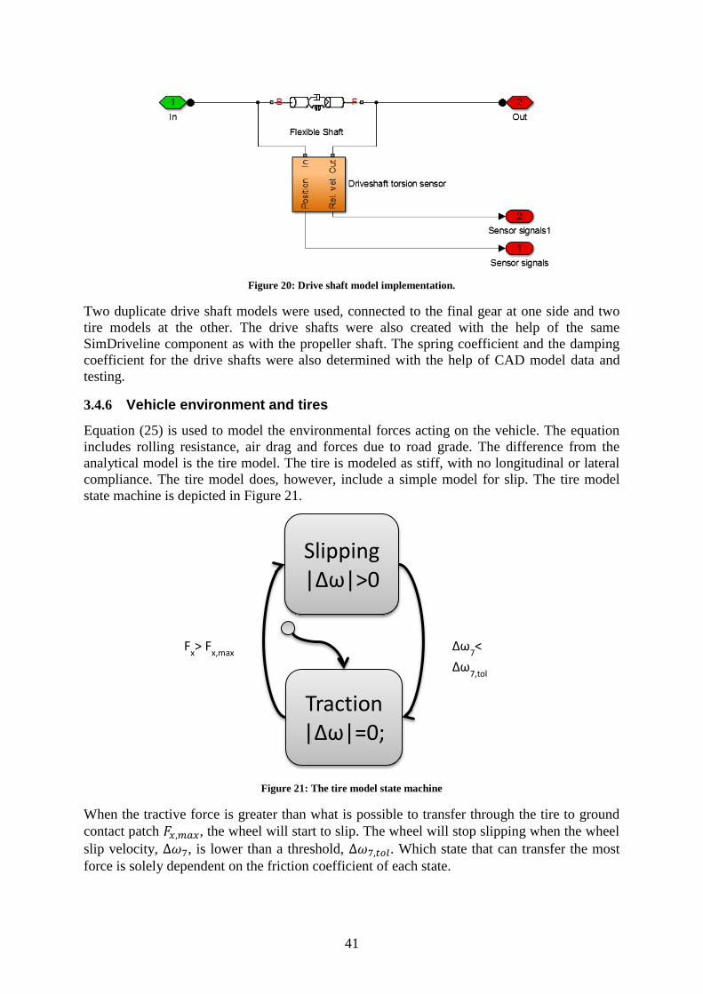
41

Figure 20: Drive shaft model implementation.

Two duplicate drive shaft models were used, connected to the final gear at one side and two

tire models at the other. The drive shafts were also created with the help of the same

SimDriveline component as with the propeller shaft. The spring coefficient and the damping

coefficient for the drive shafts were also determined with the help of CAD model data and

testing.

3.4.6 Vehicle environment and tires

Equation (25) is used to model the environmental forces acting on the vehicle. The equation

includes rolling resistance, air drag and forces due to road grade. The difference from the

analytical model is the tire model. The tire is modeled as stiff, with no longitudinal or lateral

compliance. The tire model does, however, include a simple model for slip. The tire model

state machine is depicted in Figure 21.

Figure 21: The tire model state machine

When the tractive force is greater than what is possible to transfer through the tire to ground

contact patch , the wheel will start to slip. The wheel will stop slipping when the wheel

slip velocity, , is lower than a threshold, . Which state that can transfer the most

force is solely dependent on the friction coefficient of each state.

Slipping

|Δω|>0

Traction

|Δω|=0;

Δω7<

Δω7,tol

Fx> F

x,max

42

43

4 CONTROL DESIGN

This chapter describes the control architecture and the functions of each control module in

detail with emphasis on the feedback control.

To be able to control the clutch slip some type of controller was needed. From the different

control concepts presented and briefly discussed in the frame of reference chapter, two was

chosen to further be evaluated. These were Fuzzy Knowledge Based Control and a Pole-

placed control, both with a feed forward part. The aim with the controllers was to get fast

response, with no or a small overshoot and a solid robustness to the varied driver demanded

engine torque.

4.1 Clutch control system architecture

The control system is split into multiple modules working with simple interfaces to allow

future modifications. In Figure 22 the control system is depicted, the arrows show how the

different parts of the control system interact with each other and with the plant, sensors and

actuators.

Figure 22: The control system architecture.

The signal processing and filtering stage filters all input signals and generates new signals

from the measured states; such as accelerations from measured velocities. The trajectory

planner receives the reference signal and generates a smooth slip reference that is fed into the

predictor.

Time delays are common issues with control, in some cases the control output can be out of

sync with what is actually happening in the system. This degrades performance and could

even make the controller unstable. To improve performance and robustness regarding time

delays, a predictor is implemented. The predictor is a module that takes the current input and

output states and calculates how the system would propagate if it was left with the current

input for a predefined amount of time. These “future states” are fed into the feedback control

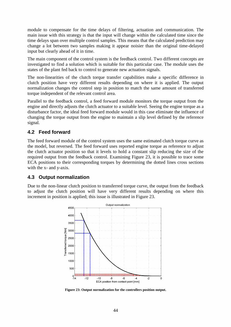
44

module to compensate for the time delays of filtering, actuation and communication. The

main issue with this strategy is that the input will change within the calculated time since the

time delays span over multiple control samples. This means that the calculated prediction may

change a lot between two samples making it appear noisier than the original time-delayed

input but clearly ahead of it in time.

The main component of the control system is the feedback control. Two different concepts are

investigated to find a solution which is suitable for this particular case. The module uses the

states of the plant fed back to control to generate new actuation signals.

The non-linearities of the clutch torque transfer capabilities make a specific difference in

clutch position have very different results depending on where it is applied. The output

normalization changes the control step in position to match the same amount of transferred

torque independent of the relevant control area.

Parallel to the feedback control, a feed forward module monitors the torque output from the

engine and directly adjusts the clutch actuator to a suitable level. Seeing the engine torque as a

disturbance factor, the ideal feed forward module would in this case eliminate the influence of

changing the torque output from the engine to maintain a slip level defined by the reference

signal.

4.2 Feed forward

The feed forward module of the control system uses the same estimated clutch torque curve as

the model, but reversed. The feed forward uses reported engine torque as reference to adjust

the clutch actuator position so that it levels to hold a constant slip reducing the size of the

required output from the feedback control. Examining Figure 23, it is possible to trace some

ECA positions to their corresponding torques by determining the dotted lines cross sections

with the x- and y-axis.

4.3 Output normalization

Due to the non-linear clutch position to transferred torque curve, the output from the feedback

to adjust the clutch position will have very different results depending on where this

increment in position is applied; this issue is illustrated in Figure 23.

Figure 23: Output normalization for the controllers position output.

45

In Figure 23, the blue dotted lines illustrate a 0.5 millimeters movement in each direction at a

position twelve millimeters from the contact point and what transferred torques it would

correspond to. The red dotted lines illustrate the same movement but at an initial position of

four millimeters from the contact point. The movement done at twelve millimeters

corresponds to a change in torque that is more than ten times as large as the same movement

done at four millimeters. This requires the controller to compensate for the non-linear

behavior to achieve the same control performance.

To avoid this problem a function is implemented which normalizes the output so that it will

have the same change in torque wherever it is applied. This function utilizes the estimated

torque transfer curve to calculate a factor with a reference point placed in the middle of the

torque range. The result will be that actuator movement applied at low clutch torques will be

amplified though at high torques the movement will be suppressed to some extent.

4.4 Trajectory control

To reduce oscillations in torque and clutch slip speed the transitions between different

reference levels are smoothened out. When demanding a new slip level, the maximum

reference acceleration is limited reducing the required output per time sample from the

feedback controller forcing it to operate with lower accelerations.

4.5 Predictor

The implemented predictor uses two different prediction algorithms depending on the current

state. The structure of the predictor is available in Figure 24.

Figure 24: Predictor structure.

If the slip speed is very low or zero a linear predictor is active. However, if the slip speed is

substantial the model based predictor is active producing better results with less noise. To

avoid excessive switching between the two models, a hysteresis is implemented to prevent

switching back to the linear predictor as long as there is a slip larger than zero. The model

based predictor does not consider the stick-slip behavior of the clutch and gives less accurate

results close to zero; this is the reason for switching to simpler prediction algorithm for low

slip velocities.

46

4.5.1 Linear predictor

The simplest version of the predictor uses the error in slip to calculate both slip acceleration

and jerk. The instantaneous derivatives of slip speed and acceleration are used to calculate the

expected change over a predefined time using linear extrapolation. Adding this change to the

current value the result is the predicted value a predefined time from now if the controller

does not change the output. This signal is then fed into the feedback controller to compensate

for the time lag in the plant model and in the communication between sensors, actuators and

control units.

4.5.2 Model-based predictor

The model based predictor is built upon a simplified version of the driveline model. Assuming

that the clutch is always slipping, the model can be split into two models, one containing the

engine dynamics and one that is the rest of the driveline. The engine model is built using

equation (49).

(49)

In equation (49), both the clutch torque and the engine torque are used as inputs. Since both

these values are calculated from other variables, the model depends on accurate estimations.

The second model, containing the rest of the driveline works in the same way and is built

using equation (50).

(50)

Worth noticing is that the simplified driveline model does not contain any stiffnesses. The

reason for this is that, during the time delay compensated for, the difference in rotational

speed due to deflection is very small.

The predictor calculates the acceleration in each point based on the given torques and uses the

Euler forward integration method to calculate the rotational speed the system would have had

if left with the current input according to equation (51).

{

(51)

where denotes the current sample and is the next sample in time. The time increment

is the sampling time of the predictor. The current sample states are always the measured

states.

4.6 Fuzzy feedback control

The fuzzy knowledge based feedback controller implemented is based on the theory from

chapter 2.3. Each module of the implemented controller is described with references to the

theory chapter.

4.6.1 Fuzzification

To control the actuator the fuzzy logic feedback uses the clutch slip velocity and the clutch

slip acceleration as inputs. Both inputs have their own set of membership function but utilizes

the same membership set structure, a typical set of membership functions are available in

Figure 25.

47

Figure 25: Fuzzy input membership function set.

In Figure 25 the different membership functions are distinguished from each other by color.

The two end functions are trapezoidal while the three middle ones are triangular functions.

The set of membership functions presented in Figure 25 fulfils equation (17). The degree of

membership to each of the five membership functions are decided for each input with its own

set of functions respectively. The five functions are named according to Table 13.

Table 13: Input membership functions

Slip velocity Slip acceleration

Too Positive + + Too Positive + +

Positive + Positive +

Perfect 0 Perfect 0

Negative – Negative –

Too Negative – – Too Negative – –

Next to the naming in Table 13 is the short name for each membership function, these will be

used to describe the inference engine.

It is also necessary to define the fuzzy set for the output; this is done according to Table 14.

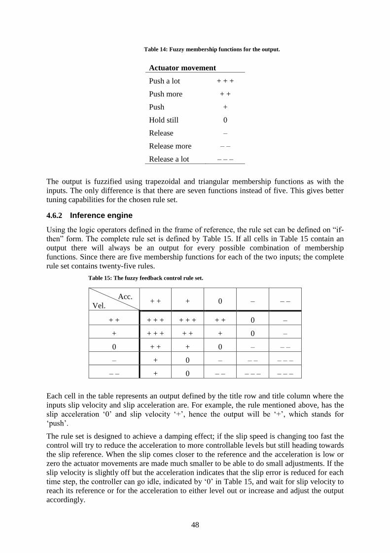
48

Table 14: Fuzzy membership functions for the output.

Actuator movement

Push a lot + + +

Push more + +

Push +

Hold still 0

Release –

Release more – –

Release a lot – – –

The output is fuzzified using trapezoidal and triangular membership functions as with the

inputs. The only difference is that there are seven functions instead of five. This gives better

tuning capabilities for the chosen rule set.

4.6.2 Inference engine

Using the logic operators defined in the frame of reference, the rule set can be defined on “if-

then” form. The complete rule set is defined by Table 15. If all cells in Table 15 contain an

output there will always be an output for every possible combination of membership

functions. Since there are five membership functions for each of the two inputs; the complete

rule set contains twenty-five rules.

Table 15: The fuzzy feedback control rule set.

Acc.

Vel. + + + 0 – – –

+ + + + + + + + + + 0 –

+ + + + + + + 0 –

0 + + + 0 – – –

– + 0 – – – – – –

– – + 0 – – – – – – – –

Each cell in the table represents an output defined by the title row and title column where the

inputs slip velocity and slip acceleration are. For example, the rule mentioned above, has the

slip acceleration ‘0’ and slip velocity ‘+’, hence the output will be ‘+’, which stands for

‘push’.

The rule set is designed to achieve a damping effect; if the slip speed is changing too fast the

control will try to reduce the acceleration to more controllable levels but still heading towards

the slip reference. When the slip comes closer to the reference and the acceleration is low or

zero the actuator movements are made much smaller to be able to do small adjustments. If the

slip velocity is slightly off but the acceleration indicates that the slip error is reduced for each

time step, the controller can go idle, indicated by ‘0’ in Table 15, and wait for slip velocity to

reach its reference or for the acceleration to either level out or increase and adjust the output

accordingly.

49

Since there will be more than one value for each output membership the maximum value is

always used to assure that the rule with highest membership always decides to the highest

extent, compared to the other rules, what the output will be.

4.6.3 Defuzzification

The process of defuzzification is done using centroid defuzzification described in chapter

2.3.5 as this is the most accurate algorithm available.

4.7 Pole placement feedback controller design

To be able to evaluate the performance of the fuzzy controller a PD controller is also

developed, this PD controller was tuned using pole placement. In order to develop the

controller, a simplified model of the linear model , which was developed in chapter 3.2, is

constructed. This model is then used to compute the closed loop polynomial which is needed

for the polynomial pole placement design. The closed loop poles are chosen to reduce the

overshoot and oscillations of the closed loop system and to reduce the effect of modeling

errors. The pole placed controller did not use the above mentioned predictor (chapter 4.5) or

output normalization (chapter 4.3) since they did not enhance the performance of this

controller.

4.7.1 Simplified Driveline Model

To be able to develop a pole placed controller a simplified version of the linear system is

developed, were the stiffnesses in the drive shafts are the only stiffnesses taken into

consideration. This is done to reduce the order of the system allowing a smaller controller

structure for the pole placement. The stiffness in the drive shafts are the main reason of

driveline oscillation, since it is the weakest stiffness in proportion to the torques affecting it ,

see chapter 2.1.2.7, and is therefore kept. The simplified model is, as the original model, only

valid for when the clutch is slipping and it does not include the communication and

computational delays or the ECA velocity limit. This means that only the slower poles and

zeroes from are modelled which can be seen in Figure 26.

50

Figure 26: Bode plot for the simplified model .

When only one stiffness is included, the order of the closed loop system is reduced and only

the first dip and peak from the Bode plot for (which can be found in chapter 3.2) is

captured in the model which can be seen in Figure 26. Thus this simplified model will give a

similar dynamic behavior as the model for frequencies below the second dip in the Bode

plot of (approximately below 200 rad/s) which the actuators control frequency will be held

beneath. The state space model corresponding to the system can be found in Appendix D.

The open loop system contains a negative integrator which means that it is unstable. To

further illustrate how the system response differs when the gear is changed, the step response

for three different gears have been plotted Figure 27. It could be seen that the slip decreases

faster with lower gears.

51

Figure 27: The step response for the continuous system which varies with the gears.

As mentioned, the system is faster for lower gears for the control frequencies in question,

however the time delays and the ECA velocity limitation remains the same for all gears which

means that the ratio between the systems time constant and delays and limitation gets larger

for lower gears. This means in turn that the system might be more difficult to control without

altering the limitations (changing the ECAs hardware/increasing the communication speed).

The closed loop systems poles represents the systems dynamic and if they can be placed

arbitrary, good control of the system dynamics could be achieved. There exists different

approaches to achieve closed loop pole control, as stated in the frame of reference (chapter

2.2); a well proven and well used one is the polynomial approach. In the polynomial approach

a desired closed loop polynomial is formed and compared with the actual closed loop

polynomial, obtaining the controller parameters.

52

4.7.2 Controller structure

When using this pole placement approach, a suitable controller structure needs to be

constructed. The controller is developed with an output feedback design, where an extra

degree of freedom is obtained compared to error feedback. The benefit of output feedback is

that the reference signal does not need to have the same type of controller structure as the

feedback signal, see Figure 28. This allows better control of the closed loop response and the

robustness to model errors and sensor noise, which is briefly discussed in chapter 4.7.2.2.

Figure 28: Output feedback and error feedback loops illustrated

Due to the fact that the open loop contained a pole in the origin and the other poles had very

low relative damping, as discussed in chapter 3.2, the controller has been designed with a PD-

like structure to dampen the overshoot and the oscillations. The oscillations needs to be

reduced since the ECA position corresponds to the clamping force which in turns represents a

large part of the dynamic torques fluctuation that are being transferred by the clutch. The

controller structure can be found in equation (52) for the Laplace domain. Compared to a

normal PD controller in the Laplace domain, two extra terms, in the numerator and

in the denominator, has been added in order to obtain the same amount of tunable

parameters as the closed loop polynomial order.

(52)

The terms and in the denominator works as filter constants and is needed in order to get

a proper transfer function for the controller. A proper transfer function is needed in order to be

able to implement the controller on the hardware.

Gc

r G

p

u y

r G

p

u y

Gff

Gc

Output feedback

Error feedback

+

-

+

-

53

The second part of the pole placed controller, the feed forward part of the feedback controller,

(which should not to be confused with the feed forward part of the controller, the torque-

position curve), has a structure according to equation (53).

(53)

This means that the feedback and feed forward part of the controller shares the same

denominator and that the transfer function from reference to output has a structure according

to equation (54).

(54)

where is the denominator in the transfer function belonging to the system , whose

state space can be found in Appendix D, and is the nominator in the plants transfer

function. The closed loop poles are represented by the denominator of , which means that

the closed loop poles can be found by setting the denominator to zero according to equation

(55).

(55)

4.7.2.1 Pole placement

The controllers parameters is found by designing a desired closed loop polynomial, according

to equation (56), and then comparing the desired closed loop polynomial with the actual

closed loop polynomial, equation (57) the Diophantine equation, and solving for the

controllers parameters.

(56)

(57)

The desired polynomial consists of two separate polynomials, the observer polynomial and

the controller polynomial , which are designed separately. The controller polynomial, ,

is chosen to acquire the closed loop response that’s desirable and the observer polynomial,

, is chosen to reduce the effect of model errors on the output.

The feed forward part of the controllers numerator, , is designed according to equation

(58).

(58)

This gives the desired closed loop transfer function that can be seen in equation (59).

(59)

As it could be seen, the observer polynomial is cancelled and its poles are not included in the

closed loop poles. The parameter , has been chosen to get a static gain of one for the closed

loop according to equations (60) and (61).

|

|

|

(60)

54

(61)

The controller polynomial, , should be of the same order as , three in this case, and

has a structure according to equation (62).

(62)

Where and are the desired poles natural frequencies and the relative damping. The

polynomial has then been chosen to acquire the same degree of the desired closed loop

polynomial as the actual closed loop polynomial, which in this case means that is of the

second order with a structure that can be seen in equation (63). The degree should be the same

because control of all the closed system poles is wanted.

(63)

In general, it is difficult to decide what the exact location of the closed loop poles should be;

there is however some general guidelines and these have been used in this project. The

relative damping of the closed loop poles should not be less than 0.7 and the poles should

have a frequency of at least one [58].

For this control design, the filter constants in the controllers transfer function, and , has

also been calculated to obtain the poles that are desired and not to filter any specific frequency

and it is important that these filter constants are positive to obtain a stable controller. To

obtain positive filter constants there is a relationship between the controller polynomial, ,

and the observer polynomial, , for each of the vehicles gear ratios that needs to be fulfilled,

this adds a constraint in how the poles can be chosen. As discussed in the frame of reference,

chapter 2.2, there are other methods developed to avoid an instable controller, however for

this project this iterative approach was considered acceptable. The higher the gear, the larger

the frequency difference between the controller polynomials, , poles and the observer

polynomials, , poles is needed to obtain a stable controller.

Since the linear model from chapter 4.7.1, , does not contain the time delays that is present

in the system, the closed loop poles has been chosen to give a slow response without any

overshoot according to the desired closed loop response. The location of the poles differs

between the gears, an example of the pole locations can be seen in Figure 29, due to the

relationship needed between and this gives different closed loop behaviors for the

different gears. In Figure 29 the closed loop poles for the twelfth gear can be seen. The poles

could not be chosen entirely freely because some pole location caused an instable controller.

For all the gears the closed loop poles (the poles belonging to the controller polynomial) were

placed around 4-6 rad/s with a relative damping of at least 0.8 and another pole around 60-100

rad/s with a relative damping of one.

55

Figure 29: Pole zero map for the continuous closed loop system for the twelfth gear.

The fastest closed loops natural frequency is at 100 rad/s (~15.9 Hz) which means a sampling

time of at least six milliseconds is required by the rule of thumb. The rule of thumb being that

the sampling time should be at least ten times the fastest pole. However this rule had to be

broken, since the sampling time in the test vehicle was fixed to ten milliseconds. The

bandwidth for the closed loop system is however around five rad/s and another rule of thumb

says that the sampling time should be ten times the bandwidth which is achieved. The closed

loop response was nevertheless dominated by the slower poles, which were below one Hertz,

and therefore this was considered to be acceptable for this study.

4.7.2.2 Model Error Sensitivity

The pole location and relative damping of the polynomial is chosen in order to reduce the

effect of possible model errors. To be able to do this, the Sensitivity function of the system

was computed according to equation (64) which is the transfer function for model errors to the

output.

(64)

The bode plot of the sensitivity function and step responses of two different observer

polynomials, , can be seen Figure 30.

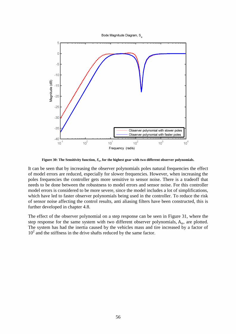
56

Figure 30: The Sensitivity function, , for the highest gear with two different observer polynomials.

It can be seen that by increasing the observer polynomials poles natural frequencies the effect

of model errors are reduced, especially for slower frequencies. However, when increasing the

poles frequencies the controller gets more sensitive to sensor noise. There is a tradeoff that

needs to be done between the robustness to model errors and sensor noise. For this controller

model errors is considered to be more severe, since the model includes a lot of simplifications,

which have led to faster observer polynomials being used in the controller. To reduce the risk

of sensor noise affecting the control results, anti aliasing filters have been constructed, this is

further developed in chapter 4.8.

The effect of the observer polynomial on a step response can be seen in Figure 31, where the

step response for the same system with two different observer polynomials, , are plotted.

The system has had the inertia caused by the vehicles mass and tire increased by a factor of

102 and the stiffness in the drive shafts reduced by the same factor.

57

Figure 31: The closed system step response for two different observer polynomials where the inertia caused by the

vehicles mass and tire has been increased by a factor of 102 and the stiffness in the drive axle has been reduced with

the same factor.

It can be seen that the controller with the faster observer polynomial is less affected by the

change in stiffness and inertia and gives a smoother response. However the faster observer

polynomial also makes the system less stable when the stiffness in the drive axle is increased,

due to the larger phase shifts the faster observer polynomial causes. The resulting sensitivity’s

function Bode plot for three different gears can be seen in Figure 32.

58

Figure 32: The sensitivity function Bode magnitude diagram for three different gears.

It could be seen that which frequency of the engine torque that affects the closed loop the

most is gear dependant and frequencies above approximately 2 rad/s has a larger effect than

frequencies below 2 rad/s.

4.7.2.3 Sampling of the controller

The pole placement has been performed in the continuous time domain, it is however not

possible to run the controller in continuous time on the hardware due to the computational

time and the actuators and sensors sampling frequency. Therefore the controller has been

approximated with Tustin approximation to discrete time. This means that the exact location

of the poles gets altered but this is considered to be acceptable for this study. However in the

future when the controller concept has been verified, it could be beneficial to design the

controller directly in discrete time, allowing better control over the poles. An example of how

the poles locations are changed when using the approximation to transfer the controller into

the z-domain can be seen in Figure 33, which is the same system as the system seen in Figure

29 where the controller has been approximated to discrete time by the Tustin approximation.

59

Figure 33: Pole zero map for the closed loop system where the controller has been approximated to discrete time by

Tustin approximation.

When comparing Figure 29 and Figure 33 it can be seen that the closed loop poles has been

moved when the approximation was used. The extra poles that appear are due to the Tustin

approximation.

The controller has so forth been designed with the linear system where the torque was

considered as the input. However the input to the system is not a torque but an ECA position

and to translate the torque demanded from the feedback controller to an ECA position the

derivative of a linear approximation of the function from torque to position (developed in

chapter 3.4.2) has been used. This approximation, a constant derivative, is a vast

simplification of the relationship between ECA position and the torque transferred by the

clutch. However this simplification proved to give better control results than more accurate

derivatives based on the ECAs’ current positions, which counteracted the controller. The

more accurate derivatives was developed to make a step in torque demanded from the

controller give the same result no matter where in the position-torque curve the ECA was, like

the output normalization for the fuzzy controller, but this led to a slower response.

4.7.2.4 Introducing an Integral part to the Controller

The Pole-placed PD controller gives an acceptable result when the measured torque-position

curve for the ECA and clutch is approximately known and used in the feed forward part of the

controller. When an error is introduced in the torque-position curve in the feed forward

controller the PD controllers response resulted in a static error, both in the model and in the

vehicle. This is expected, however the amplitude of the static error is larger than acceptable

when the controller is implemented in the vehicle and an already implemented adapted

torque-position curve is used instead of the torque-position curve developed during this thesis.

If an implementation in more vehicles than the current test vehicle should be made, the fitted

torque-position curve that has been developed during this thesis will not be accurate. To

60

compensate for the error and to reduce the static error a slow integral part is added to the

controller. This eliminated the static error but caused a slightly more oscillating closed loop

system. The integrator is introduced in parallel to the pole placed controller in order to get a

faster implementation. The implementation of the integral part to the controller led to a new

closed loop structure, which can be found in equation (65) and the new feedback controller

structure can be seen in Figure 34.

Figure 34: The new feedback controller structure

Note, that the new controller has a negative sign in equation (65) due to the input to the new

controller is the measured slip with the reference slip subtracted and the pole placed controller

has the input the other way around, the reference slip with the measured slip subtracted.

(65)

The integrals gain was iteratively tuned and altered the closed loop poles which can be seen in

Figure 35 for the twelfth gear. It can be seen that the poles have become slower. It could also

be seen that some of the pole zero pairs that’s previously cancelled each other, now does not

cancel each other.

Gc2

r G

p

u y G

ff

Gc1

- +

+

- +

+

61

Figure 35: The pole zero map for the closed loop system with the integral part for the twelfth gear.

This also renders a new model error sensitivity function which is defined in equation (66) and

the frequency behavior for the sampled sensitivity function can be seen in the Bode plot in

Figure 36.

(66)

This variant of the pole placed controller with an added integrator will further on be

referenced to as the pole placed based controller (PPBC).

62

Figure 36: The new sensitivity functions Bode magnitude diagram for three different gears for twelfth gear.

It could be seen that the new controllers’ sensitivity function has similar behavior to the old

controllers sensitivity function.

4.8 Filter design

To avoid sensors noise and to eliminate the constant slip fluctuation caused by the firing

pulses that cannot be reduced without a faster sampling frequency, a low pass filter is

implemented. A second order Butterworth filter is constructed with a break frequency of 10

Hz and a sampling frequency of 100 Hz. The Bode plot for the filter can be seen in Figure 37,

where it could be seen that at 10Hz (~62.8 rad/s) that the gain is -3 dB. The break frequency

was chosen to be ten times slower than the sampling frequency, according to a rule of thumb.

The Butterworth filter is chosen as filter type since it is relative easy to implement and a

second order Butterworth filter is used in order to get a steeper derivative by the break

frequency than what a first order Butterworth filter would have. The filter causes a phase lag

of approximately 90 degrees which causes a slower response from the controller. A higher

order filter is not used since this would cause an even larger phase lag.

63

Figure 37: The Bode plot of the digital filter implemented in the control loop.

4.9 Engine PI-controller

In order to be able to control the slip at low gears, an engine torque PI controller is

implemented in parallel to the ECAs controllers. The engine PI controller is tuned by a kind

of Ziegler-Nichols like procedure in the simulated model. The output from the engine torque

controller is sent to the feed forward part of the ECA controllers in order to make sure that

these two controllers do not work against each other. This is illustrated in Figure 38.

Figure 38: The combined engine and ECA controller structure.

4.10 Powertrain parameter variation

In order to investigate how different critical powertrain parameters affected the controller

performance, simulations are conducted where the parameters are altered and the controller

64

results evaluated. These are performed at the first gear since the slip is most difficult to

control at the first gear. This is because of the slip is less dampened at the lower gears because

of the higher gear ratios as discussed in chapter 3.2 and chapter 4.7.1.

4.11 Implementation

To be able to measure the controllers’ performance in a heavy duty truck the controllers had

to be adapted to be able to work with the existing software in the test vehicle. This was

accomplished by changing the Simulink blocks into Simulink Scania Standard blocks to

ensure the correct syntax and to be able to generate the code that would be running on the

ECUs. The ECUs has a limited amount of memory and to be able to reduce the risk of

overflow the memory a review of each of the variables data types had to be made. This was

performed by identifying the necessary precision needed for all the variables used and

changing the data type to the smallest possible. The code was then auto generated from

Simulink into c-code which in turn was compiled and run on the ECUs.

Compared to the simulated controller, the controller implemented in the vehicle’s feed

forward part uses a torque-position curve which had been adapted in the already implemented

software on the ECU. This lowered the performance of the controller somewhat in some cases

but was considered necessary if the implementation should be able to run in more vehicles

than the test vehicle used in this project. The controllers were tested in a vehicle whose

adaptations were erased when the controllers’ software was programmed in the ECU. This

will probably affect the performance of the torque curve adaptations.

65

5 RESULTS

The results chapter is divided into three parts; model verification results, controller results

and finally parameter variation results.

5.1 Model results

The verification of the model has been performed by evaluating the physical signals in the

model and comparing these to the sampled signals obtained during tests in the test vehicle

Fronda. The physical signals have been sampled with the help of existing sensors and

software in the powertrain.

5.1.1 Engine

The engine model consists of a modeled inertia, a measured average engine torque signal and

a sinusoidal wave that has been added to the average torque signal in order to simulate the

firing pulses. To verify the modeled inertia a test was performed where the engine crankshaft

speed was logged. The test was made when the vehicle was not moving, the clutch was

opened and the accelerator pedal was pushed.

It can be seen in Figure 39 that the dynamical behavior of the engine velocity is close to the

real system. A difficulty with verification of the inertia is that this verification is depending on

that the reported engine torque, which is an observed state, is correct. The engine torque

observation is thoroughly developed and is widely used within Scania. There is however still

a risk that the reported torque might differ from the actual torque, which could cause

deviations between the model behavior and the sampled data.

66

Figure 39: The engine angular velocity in the model and measured while pushing the accelerator with an open clutch

for four different driving scenarios.

The test was performed for eight times, of which four has been plotted, which should reduce

the risk of noise or trends dominating the results. The reported average engine torque was

then used as input to the simulated model and the engine velocity was measured. A mean

deviation was calculated and minimized for the eight cases which led to a small alteration of

the previously calculated inertia.

The firing pulses modeled were evaluated by studying previous tests and comparing the

frequency of the torque frequency after the clutch in the model with the test results. The

amplitudes of these are difficult to verify since the measurement point is after the clutch and

the actuator (engine) is placed before. The large inertias, spring and damper causes changes in

the torque amplitude and the measured torque amplitude after the clutch is therefore not the

same as the torque amplitude from the engine. However, if the powertrain inertia and

67

damping is correctly modeled, the amplitude caused by the firing pulses of the torque should

be the same in the model as in the vehicle by the gearbox input shaft. The torque’s frequency

is the same on both sides of the clutch. By comparing the measured torque after the clutch in

the model with the sampled data in Figure 40, it can be seen that the simulated frequency is

very close to the real system but slightly phase shifted. The model has the same average

engine torque as the real engine, but because of the simple model the shape of the wave and

amplitude is slightly different. The shape of the actual wave is caused by the three injection

stages; pre-injection, main injection and post-injection.

Figure 40: A short time frame of the torque transferred by the clutch, measured in a vehicle and simulated in

Simulink. The effects of the ignition pulses are clearly visible.

It can be concluded that the engine model represents the behaviour of the real system that is of

interest when developing the controller algorithm. The modeled engine has a rapidly

fluctuating torque, with a frequency and amplitude that is close to the real system, and the

corresponding acceleration as output.

68

5.1.2 Electronic Clutch Actuator

The Electronic Clutch Actuator (ECA) speed and delay was mapped against the measured

signals, see chapter 3.4.2. Examining Figure 41, the movement of the clutch actuator closely

resembles the measured results.

Figure 41: Measured and simulated ECA movement.

The biggest difference is the inertia of the systems; the measured actuator brakes due to its

internal position control when it approaches the reference at high velocity while the simulated

actuator does not. This is most clear between three and five seconds in Figure 41. When

controlling a clutch slip there will mostly be small adjustments as the torque from the engine

varies, as between six and nine seconds in Figure 41. It is evident that the inertia of the system

becomes less important in this case and the simulated actuator matches the real system very

well. The zoomed area shows that the system is mostly dependent on its delay and not its

inertia when small adjustments are made in the reference position.

5.1.3 Clutch

The sampling rate of the measureable velocity sensors is low compared to the dynamics of the

clutch; it is therefore difficult to assess how the clutch model compares to the real system in

the stick-slip area. The velocity tolerance in the model, see chapter 3.4.2, has been chosen to

represent the actual behaviour of the clutch.

The least squares fitted position to torque polynomial presented in chapter 3.4.2 as equation

(22) is validated for new transferred torque data, displayed in Figure 42.

69

Figure 42: Clutch transferred torque validation.

The new data is scattered around the torque curve used in the simulations. Since the new data

fits well with the approximation it can be concluded that the clutch torque transferability is

well tuned and works as expected. The outliers that can be seen in the plot are disregarded

since they are considered to be erroneous.

Figure 43: Clutch torque transfer as a function of actuator position with samples colored by estimated temperature.

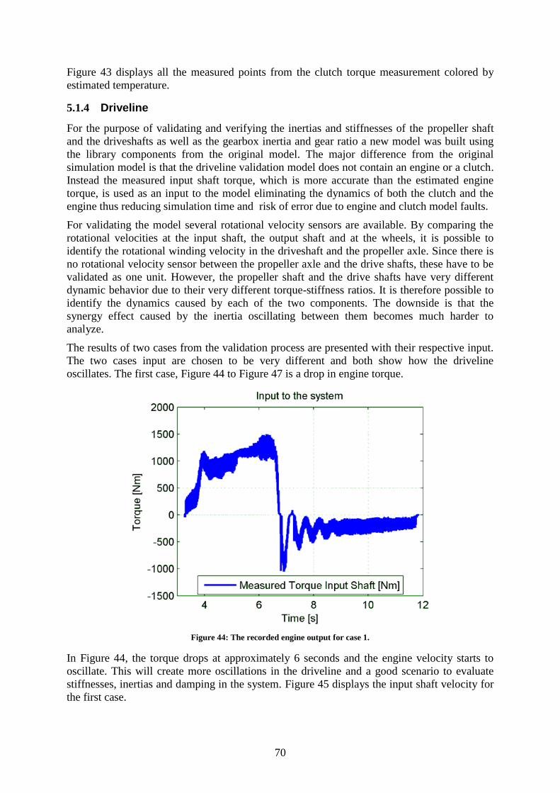
70

Figure 43 displays all the measured points from the clutch torque measurement colored by

estimated temperature.

5.1.4 Driveline

For the purpose of validating and verifying the inertias and stiffnesses of the propeller shaft

and the driveshafts as well as the gearbox inertia and gear ratio a new model was built using

the library components from the original model. The major difference from the original

simulation model is that the driveline validation model does not contain an engine or a clutch.

Instead the measured input shaft torque, which is more accurate than the estimated engine

torque, is used as an input to the model eliminating the dynamics of both the clutch and the

engine thus reducing simulation time and risk of error due to engine and clutch model faults.

For validating the model several rotational velocity sensors are available. By comparing the

rotational velocities at the input shaft, the output shaft and at the wheels, it is possible to

identify the rotational winding velocity in the driveshaft and the propeller axle. Since there is

no rotational velocity sensor between the propeller axle and the drive shafts, these have to be

validated as one unit. However, the propeller shaft and the drive shafts have very different

dynamic behavior due to their very different torque-stiffness ratios. It is therefore possible to

identify the dynamics caused by each of the two components. The downside is that the

synergy effect caused by the inertia oscillating between them becomes much harder to

analyze.

The results of two cases from the validation process are presented with their respective input.

The two cases input are chosen to be very different and both show how the driveline

oscillates. The first case, Figure 44 to Figure 47 is a drop in engine torque.

Figure 44: The recorded engine output for case 1.

In Figure 44, the torque drops at approximately 6 seconds and the engine velocity starts to

oscillate. This will create more oscillations in the driveline and a good scenario to evaluate

stiffnesses, inertias and damping in the system. Figure 45 displays the input shaft velocity for

the first case.

71

Figure 45: Input shaft velocity for case 1.

The difference between measured input shaft velocity and measured engine velocity in Figure

45 indicates that the clutch is slipping. In this simulation, the clutch dynamics are not

simulated and the clutch is considered to be locked during the entire simulation. The

simulation model exhibits a smaller damping than the actual system but oscillates with the

same frequencies as the real system. Chapter 1.6 (system introduction) describes that the

layshaft velocity is measured to calculate the input shaft velocity, in other words is the

measured result subject for unwanted dynamics and lower resolution. Further on, Figure 46

displays the output shaft velocity.

Figure 46: Output shaft velocity for case 1.

72

The simulated output shaft velocity shows the same dynamics as the input shaft because of the

rigid gearbox model. The reason for the delay in time when comparing the measured output

shaft with the simulated result is because of filtering. Figure 47 shows the vehicle velocity

measured with the ABS sensors at both the front and rear axle together with the simulated

result for the rear driven axle.

Figure 47: Vehicle velocity for case 1.

Since the simulation is engine driven, the vehicle velocity is the velocity that is furthest away

from the actuation point. The fact that the measured front and rear velocities coincide

indicates that the rear axle is not slipping or that both axles are slipping, while the latter is

highly unlikely because of good road conditions.

The second case, presented in Figure 48 to Figure 51 is an oscillating torque from the engine

which gives a lot of dynamics in the driveline.

73

Figure 48: Engine output for case 2.

Figure 48 shows the engine velocity and the engine torque output. While torque levels are

moderate to high the engine struggles to maintain velocity. The reason for this is that the

measurement was done while going uphill. Figure 49 displays the same behaviour.

Figure 49: Input shaft velocity for case 2.

Here, the simulated input shaft velocity has a varying offset compared to the measured

velocities but oscillates with the same frequencies and a somewhat higher amplitude. The

offset exist solely in simulations based on measurements conducted where the road grade

74

changes rapidly. Since the road grade input to the simulations the recorded vehicle online road

grade estimation the results will differ momentarily as the signal is low pass filtered. Figure

50 displays the same offset for simulated velocities as Figure 49.

Figure 50: Output shaft velocity for case 2.

The simulation shows a higher amount of noise compared to the measured velocities for low

engine velocities and torques above 800 Nm. This indicates that the simulation model has

lower damping than the real system, which is also indicated in Figure 45. The problem with

offset is also evident in Figure 51.

Figure 51: Vehicle velocity for case 2.

75

The offset is however not a problem for control design, as long as the proper dynamics of the

driveline can be modelled. The damping constant is intentionally left a little lower than the

measured system suggests. A lower damping puts a higher demand on the control and this

suggests that the transition from model to real system will be easier. It can be concluded that

the calculated inertias and stiffnesses in the simulation model gives an acceptable dynamical

result.

5.1.5 Environmental forces

The rolling resistance and air resistance was tested by rolling from high velocities with neutral

gear until lower velocities, a coast down test, which can be seen in Figure 52 and Figure 53.

Unfortunately the road where this test was performed were slightly inclined which will affect

the speed of the vehicle. To compensate for this the test was performed in both directions and

the road incline data was logged and used as input to the simulated model.

The rolling resistance was first set to a value obtained from Eriksson et al. [59] and then tuned

using an automated (scripted) iterative process to minimize the absolute value of the

difference between the modelled vehicle speed and the measured vehicle speed for the entire

coast down test performed. The drag coefficient was tuned in a similar way, but with only the

high speed coast down test used to increase the influence of the drag force, see Figure 53.

When calculating the drag and rolling resistance with this approach, the rolling resistance and

drag will compensate for other unmodeled losses in the powertrain which for this study is

considered to be acceptable. The drag constant will also compensate for possible erroneous

frontal area estimation.

76

Figure 52: The results from a coast down tests performed in both directions of a slightly inclined road compared with

the corresponding simulated result.

77

Figure 53: The results from a coast down tests performed in both directions of a slightly inclined road compared with

the corresponding simulated result.

There is a deviation between the simulated speed and the measured speed, especially in the

upper plot in Figure 52 and Figure 53. This deviation may be explained by a faulty incline

measurement and is not considered as a critical risk when developing the controller.

Validating the rolling resistance has been performed by comparing the values obtained with

values found in the literature. The obtained values are a slightly higher than the ones found in

the literature [59], this could be explained by the unmodeled losses, for example churning and

bearing friction, that the obtained values are compensating for.

78

5.2 Simulated controller results

In this chapter the results obtained from simulations are presented. The controllers were

evaluated by using a constant slip reference input and tested how they could compensate for

disturbances caused by a step in engine torque. The controllers are tested for gear seven and

gear eleven. Gear seven is the lowest gear that the slip control could handle with an

acceptable result. Gear eleven is used as reference to point out differences in controllability

between different gears.

5.2.1 Two degree of freedom controller design

The pole placed controller was first designed as a PD controller; this led to a static error when

the torque position curve was not accurate, which can be seen in Figure 54. In the simulation,

which led to the results that can be seen in Figure 54, an error of 0.5 mm has been introduced

in the feed forward controllers torque-position curve. This size of error could be expected

when the controller is implemented in a vehicle. As it could be seen, the error was too large

for the controller to be useable if a slip reference below approximately 100 rpm should be

used. In the torque plot the firing pulses impact on the transferred torque can be seen before

and while the clutch is slipping. At about three seconds the clutch is definitely in slip mode

and the transferred torques amplitude is significantly decreased.

Figure 54: The pole placed PD controllers simulated step response when an error (0.5 mm) in the torque-position

curve that is used in the engine torque feed forward controller has been introduced.

To compensate for this, an integrating part was added to the controller which eliminated the

static error but led to a slightly more oscillating system. The same engine torque and road

Simulated

Reference

79

inclination signal were used when the pole placed PD controller with an added integrator (the

PPBC) was tested in another simulation. The result of this simulation can be seen in Figure 55

and it can be seen that the static error has been eliminated.

Figure 55: The pole placed PD controller with an added integrating parts simulated step response when an error (0.5

mm) in the torque-position curve that is used in the engine torque feed forward controller has been introduced.

5.2.2 Step in slip velocity with ramps in torque

The torque input to the simulations mimics cruising at a constant velocity and then activating

the controller. It is then evaluated how well the controllers respond to changes in torque from

the engine. The control performance is evaluated for the seventh and the eleventh gear. The

gears were chosen to properly illustrate the controllers’ behaviour on a stable gear, the

eleventh gear, and a gear where the controllers were close to being unstable, the seventh gear.

5.2.2.1 7th gear

The slip velocity for the PPBC control is displayed in Figure 56.

Figure 56: Simulated slip velocity for PPBC control at the seventh gear.

In Figure 56 the control quickly establishes a slip after the control is activated. The rise and

settling times are long as the control algorithm undershoots with approximately 40 percent at

about 5 seconds. Worth noting is the increase in noise that appears at 6 seconds. In Figure 57

the engine output torque and the clutch transferred torque are depicted.

Simulated

Reference

Simulated

Reference

80

Figure 57: Simulated torques for PPBC control at the seventh gear.

From Figure 57 it is evident that the noise appears when the torque level changes, when the

torque is ramped down to lower levels towards the end of the simulation, the noise level

descends. In Figure 58, the requested actuator position from control is plotted with the actual

position of the actuator.

Figure 58: Simulated actuator position for PPBC control at the seventh gear.

In Figure 58, the control signal moves fast towards an approximate position because of the

feed forward part. Knowing that the slip reference is constant throughout the simulation, the

changes in torque are directly visible on the actuator position. As the torque increases, the

actuator pushes harder, decreasing its position, to enable the clutch to transfer more torque to

maintain the slip velocity.

The FKBC response in slip velocity is depicted in Figure 59.

81

Figure 59: Simulated slip velocity for FKBC control at the seventh gear.

As with PPBC control, the FKBC exhibits high noise levels when the torque changes to

higher levels. It can also be seen that the FKBC has a much shorter rise time than the PPBC

but overshoots with approximately 40 percent and undershoots with 40 percent as well. The

engine torque and the clutch transferred torque for the FKBC are presented in Figure 60.

Figure 60: Simulated torques for FKBC control at the seventh gear.

The transferred torque in Figure 60 resembles that of Figure 57. The dynamics from the

engine almost disappear as the clutch opens at 2 seconds. Figure 61 shows the control signal

and the actuator position for the FKBC.

Figure 61: Simulated actuator position for FKBC control at the seventh gear.

Simulated

Reference

82

Figure 61 resembles Figure 58 because of the same feed forward module. Only the small

adjustments in position made by the feedback control will differ.

5.2.2.2 11th gear

The slip velocity for the PPBC control at the eleventh gear is displayed in Figure 62.

Figure 62: Simulated slip velocity for PPBC control at the eleventh gear.

The noise levels become much larger when the torque is increased. The step response features

a several percent of undershoot and much shorter rise and settling time compared to the

seventh gear using the same algorithm. The transferred torque in Figure 63 follows the engine

torque.

Figure 63: Simulated torques for PPBC control at the eleventh gear.

The firing pulse dynamics are much smaller when the clutch slips in Figure 63 as well. The

PPBC requested actuator position is pictured in Figure 64 with the actual position of the

actuator.

Simulated

Reference

83

Figure 64: Simulated actuator position for PPBC control at the eleventh gear.

Worth noticing in Figure 64 is the feedback response after the feed forward has moved the

actuator to the correct region. To get a slip, the actuator releases marginally and as the clutch

velocity increases the clutch engages again to stabilize the slip velocity at the reference level.

The FKBC slip velocity is displayed in Figure 65.

Figure 65: Simulated slip velocity for FKBC control at the eleventh gear.

Here, the control starts to oscillate heavily when the torque increases but the oscillations are

reduced when the torque is ramped down. In Figure 66, the transferred torque and the engine

torque for the FKBC at the eleventh gear are presented.

Figure 66: Simulated torques for FKBC control at the eleventh gear.

Simulated

Reference

84

The oscillations in Figure 65 can clearly be seen in Figure 66 as well but compared to the

firing pulses at 200 Nm static engine output the amplitude of the oscillations are still smaller.

The cause of the oscillations can be seen in Figure 67.

Figure 67: Simulated actuator position for FKBC control at the eleventh gear.

In Figure 67, the actuator requested and actual positions are graphed. It is clear that the

oscillations in both transferred torque and slip velocity come from overcompensation in the

feedback control. Considering Figure 16 the same movement corresponds to a much larger

change in torque when the clamping force on the clutch is high. This means that the accuracy

of both the hardware and the control decreases with higher torques.

5.3 Robustness of the controllers

As, discussed, both the Fuzzy controller and the pole placed based controller, PPBC, worked

when the model parameters were known while the tuning of the controllers was performed.

To verify the robustness of the controllers to model errors, simulations were run with a

change in the driveline parameters. The parameters that were considered to have the most

influence on the powertrain’s behaviour are the vehicle mass and the stiffness of the drive

axles. The controllers were more sensitive to smaller vehicle mass and less stiff drive shafts

compared to an increase in one of these. An increased vehicle mass, created a more dampened

system Therefore simulations were run where the mass and stiffness were set to a fourth

respective the half of the original value. The values were chosen to be values that might be

actual parameters for different vehicles, half the stiffness in the drive shafts and a fourth of the

mass. The results can be seen in Figure 68 and Figure 69 for the PPBC and the FKBC

respectively.

85

Figure 68: The simulated result when the drive shafts stiffness has been half of the original value and the vehicles

mass to a fourth of its original value. The PPBC has been evaluated.

Simulated

Reference

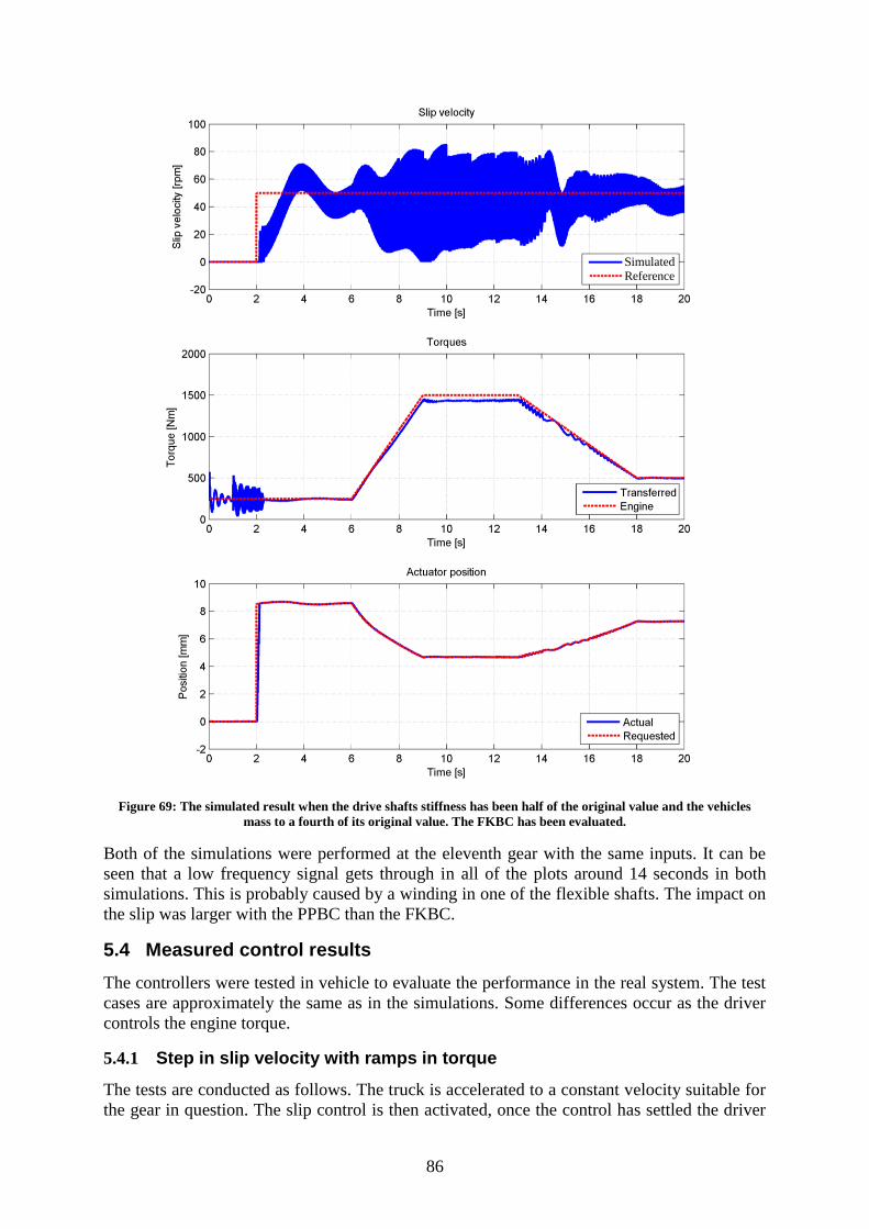
86

Figure 69: The simulated result when the drive shafts stiffness has been half of the original value and the vehicles

mass to a fourth of its original value. The FKBC has been evaluated.

Both of the simulations were performed at the eleventh gear with the same inputs. It can be

seen that a low frequency signal gets through in all of the plots around 14 seconds in both

simulations. This is probably caused by a winding in one of the flexible shafts. The impact on

the slip was larger with the PPBC than the FKBC.

5.4 Measured control results

The controllers were tested in vehicle to evaluate the performance in the real system. The test

cases are approximately the same as in the simulations. Some differences occur as the driver

controls the engine torque.

5.4.1 Step in slip velocity with ramps in torque

The tests are conducted as follows. The truck is accelerated to a constant velocity suitable for

the gear in question. The slip control is then activated, once the control has settled the driver

Simulated

Reference

87

applies torque from the engine to disturb the control. To be able to do comparisons, the tests

are conducted for the seventh and eleventh gear as with the simulations.

5.4.1.1 7th gear

The measurement for the PPBC control in seventh gear shows some differences compared to

the simulated result. In some cases, such as in Figure 70 the control overshoots when the

control is activated.

Figure 70: Measured slip velocity for PPBC control at the seventh gear.

By comparing Figure 70 and Figure 71 it is clear that the control fails to keep the clutch

slipping when the driver applies full acceleration, but it recovers its slip after about one

second. To settle, takes almost 4 seconds.

Figure 71: Measured torques for PPBC control at the seventh gear.

At the 90 second mark in Figure 71 the clutch sticks and all torque dynamics from the engine

are transferred to the driveline by the clutch. The recorded control signal and actuator signal is

available in Figure 72.

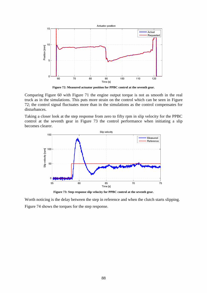
88

Figure 72: Measured actuator position for PPBC control at the seventh gear.

Comparing Figure 60 with Figure 71 the engine output torque is not as smooth in the real

truck as in the simulations. This puts more strain on the control which can be seen in Figure

72; the control signal fluctuates more than in the simulations as the control compensates for

disturbances.

Taking a closer look at the step response from zero to fifty rpm in slip velocity for the PPBC

control at the seventh gear in Figure 73 the control performance when initiating a slip

becomes clearer.

Figure 73: Step response slip velocity for PPBC control at the seventh gear.

Worth noticing is the delay between the step in reference and when the clutch starts slipping.

Figure 74 shows the torques for the step response.

89

Figure 74: Step response torques for PPBC control at the seventh gear.

By comparing Figure 73 and Figure 74 it is clear that the transferred torque is proportional to

the slip acceleration, when the slip velocity derivative is high, the difference between

transferred torque and engine torque is large. Figure 75 shows the actuator position for the

step response.

Figure 75: Step response actuator position for PPBC control at the seventh gear.

Since the transferred torque is almost proportionally related to the actuator position, the

transferred torque follows the same pattern as the actuator position.

The FKBC measurement in Figure 76 exhibits a much more oscillative behavior than the

PPBC controller for the same case in Figure 70.

90

Figure 76: Measured slip velocity for FKBC control at the seventh gear.

As with the PPBC control, the ramp in engine torque cannot be handled correctly by the

control algorithm although the FKBC never appears to be sticking. By analyzing Figure 77,

the transferred torque appears noisier than with the PPBC control in Figure 71.

Figure 77: Measured torques for FKBC control at the seventh gear.

The noise has the same source as in the simulations, which is evident from Figure 78 where

the requested actuator position oscillates when the feedback control overcompensates.

Figure 78: Measured actuator position for FKBC control at the seventh gear.

From Figure 78 and Figure 72 it is clear that the feed forward module works well with the real

system as well as the simulations in Figure 58 and Figure 61.

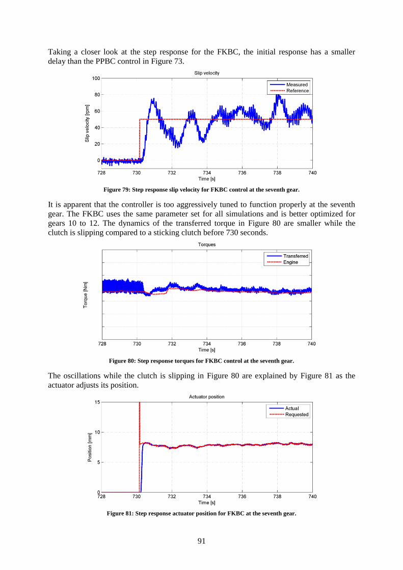
91

Taking a closer look at the step response for the FKBC, the initial response has a smaller

delay than the PPBC control in Figure 73.

Figure 79: Step response slip velocity for FKBC control at the seventh gear.

It is apparent that the controller is too aggressively tuned to function properly at the seventh

gear. The FKBC uses the same parameter set for all simulations and is better optimized for

gears 10 to 12. The dynamics of the transferred torque in Figure 80 are smaller while the

clutch is slipping compared to a sticking clutch before 730 seconds.

Figure 80: Step response torques for FKBC control at the seventh gear.

The oscillations while the clutch is slipping in Figure 80 are explained by Figure 81 as the

actuator adjusts its position.

Figure 81: Step response actuator position for FKBC at the seventh gear.

92

At 730 seconds in Figure 81 it is possible to see the effects of the maximum actuator velocity

as the actual position lags behind the requested position.

5.4.1.2 11th gear

As seen in Figure 82, the PPBC control gives much better results for the eleventh gear than

for the seventh gear in Figure 70; this applies both for the simulated and the measured results.

Figure 82: Measured slip velocity for PPBC control at the eleventh gear.

The same issues appear in the real truck as with the simulations. When the torque from the

engine increases, the slip velocity starts to oscillate. It is also worth noticing the behavior in

slip speed when the ramp in engine torque is applied in Figure 83.

Figure 83: Measured torques for PPBC control at the eleventh gear.

Studying Figure 83, the torque oscillations when the torque is ramped up appear in the real

system as well as in the simulations in Figure 62. By studying the control signal and actuator

position in Figure 84 the source of the oscillations are found.

93

Figure 84 Measured actuator position for PPBC control at the eleventh gear.

When the torque reaches high levels, the control starts to oscillate but regains damping as the

torque is ramped down.

Looking closer at the step response for the PPBC control, the result is much better for the

eleventh gear in Figure 85 than for the seventh gear in Figure 73.

Figure 85: Step response slip velocity for PPBC control at the eleventh gear.

The recorded overshoot is much smaller for the eleventh gear in Figure 85 than for the

seventh in Figure 73. The transferred torque is also smoother for the recording represented by

Figure 86 than recording represented by Figure 74.

Figure 86: Step response torques for PPBC control at the eleventh gear.

94

The velocity of the actuator in Figure 87 will have a larger effect on the step response for low

torques as the actuator will have to move from closed to the corresponding transferred torque

which is decreasing as the actuator moves towards the contact point, see Figure 43.

Figure 87: Step response actuator position for PPBC control at the eleventh gear.

The actuator moves slightly to adjust the slip velocity but no major corrections are done.

The FKBC slip velocity in Figure 88 exhibits the same oscillations for high engine torques as

the other simulated and measured cases.

Figure 88: Measured slip velocity for FKBC control at the eleventh gear.

The engine torque and clutch transferred torque in Figure 89 shows that the slip velocity is

closely related to the transferred torque.

95

Figure 89: Measured torques for FKBC control at the eleventh gear.

Studying the time 325 to 332 seconds in Figure 89 the engine outputs torques which are close

to its maximum output. At this point the slip velocity in Figure 88 oscillates both with large

amplitude and higher frequency than for torques which are required to maintain vehicle

velocity for the test conditions.

Further on, Figure 90 displays the measured actuator position

Figure 90: Measured actuator position for FKBC control at the eleventh gear.

It can be seen that the oscillations in slip velocity and torque are induced by the control, as the

actuator starts to move back and forth, the transferred torque will follow the same behaviour

and directly affecting the slip acceleration.

The FKBC step response for the eleventh gear is available in Figure 91.

96

Figure 91: Step response slip velocity for FKBC control at the eleventh gear.

The FKBC produces a stable response at the eleventh gear. In Figure 91 the slip velocity

peaks at 70 rpm before the derivative changes sign. In Figure 92 the corresponding torques

can be found.

Figure 92: Step response torques for FKBC control at the eleventh gear.

The transferred torque is smoother when the clutch slips as with all other cases and better than

the seventh gear where the control oscillates more and creates its own dynamics.

Figure 93: Step response actuator position for FKBC control at the eleventh gear.

The FKBC makes more and larger adjustments in Figure 93 than the PPBC control in Figure

87.

97

5.4.1.3 Fourth gear with engine control

The control has proved to work better the higher the gear. To be able to control the slip level

at starting gears an experimental engine control is introduced to accompany the PPBC clutch

control. Figure 94 displays the slip velocity for this control at the fourth gear.

Figure 94: Measured slip velocity for PPBC clutch control with PI engine control at the fourth gear.

Studying Figure 94 it is evident that the control is not entirely stable. The first fifteen seconds

shows the result with a slip velocity reference of 50 rpm, this is however not enough to keep

the clutch slipping. When the reference is changed to 150 rpm, the control has a higher

tolerance for errors in control.

Figure 95: Measured torques for PPBC clutch control with PI engine control at the fourth gear.

In Figure 95 the driver does not move the acceleration pedal. The small fluctuations in engine

torque are mostly made by the PI engine control compensating for errors in slip velocity. The

clutch actuator position and clutch control reference in Figure 96 shows more aggressive

movements than in Figure 72 and Figure 84 where PPBC control is applied for the seventh

and eleventh gears.

98

Figure 96: Measured actuator position for PPBC clutch control with PI engine control at the fourth gear.

Comparing Figure 94 with Figure 96 it can be seen that most oscillations originate from the

clutch control and how the clutch moves.

5.5 Powertrain parameter variation

In order to investigate how the slip controllers’ performance could be enhanced, selected

powertrain parameters were varied in the simulation environment while the PPBC was

controlling the system. The system parameters that reduced the performance of the controllers

the most were considered to be the delays in the system, both the computational time in the

ECAs ECU and the transport delays caused by CAN and the winding in the drive shafts. To

verify how the different parameters affected the slip velocity, simulations were made where

these parameters were altered. The improvement was then evaluated by comparing the clutch

slip controllers’ performance, when only the ECA is controlled and not the engine torque, at

the first gear for different setups. As a reference the simulated controller performance for the

current driveline parameter setup can be found in Figure 97.

99

Figure 97: The reference and actual slip velocity, the average engine torque and the torque transferred by the clutch,

the actuator reference and position plotted. These results were obtained while simulating the PPBC working at the

first gear.

The reference driving situation was chosen to be one where there were initial oscillations in

the driveline (which can be seen on the transferred torque before the reference slip velocity

step) and where a constant torque (200 Nm) was held as the output from the engine for the

first ten seconds. Then the engine torque was ramped during one second until 500 Nm and

then again held constant. In the simulation a road incline has also been used to make the

driving scenario more realistic, the inclination has first been held constant then increased at 10

seconds. It could be seen that the controller could not control a slip properly at the first gear

for the current powertrain setup, which has been verified in vehicle tests.

The communication delays caused by the CAN caused delays both from the engine velocity

sensor into the controller and out from the controller to the actuator. If these could be reduced,

100

it would create a system which would be easier to control. Therefore the delay caused by the

CAN was reduced in the simulations to find a possible delay where the controller was

effective. To only reduce the CAN delay was not however enough, which could be suspected,

to be able to control the slip at the first gear, the total delay from controller to actuating was

still too large due to the ECA computational delay. However, after reducing the ECA delay to

0.1 ms and the CAN delay to 0.1 ms (which meant that the total delay from controller to

actuator where 2% of the sampling time) the slip could be controlled by only controlling the

ECA, which can be seen in Figure 98.

Figure 98: The reference and actual slip velocity, the average engine torque and the torque transferred by the clutch,

the actuator reference and position plotted. These results were obtained while simulating the PPBC working at the

first gear with very small delays.

101

The winding in the driveline also caused problems for the controllers, the largest winding was

found in the drive shafts. In order to reduce the amplitude of the drive shafts oscillations,

these were made stiffer. In Figure 99 and Figure 100 the controller performance can be seen

when the stiffness in the drive shafts has been doubled. It could be seen that the slip speed is

less oscillating than before and the initial overshoot is gone.

Figure 99: The reference and actual slip velocity, the average engine torque and the torque transferred by the clutch,

the actuator reference and position plotted. These results were obtained while simulating the PPBC was working at

the first gear and stiffer drive shafts were simulated.

Though the stiffer drive shafts improves the controllers performance slightly, the slip still

could not be controlled when the engine torque is increased and the current delays were

102

simulated, therefore a simulation was performed where both the drive shafts were stiffer and

the delays smaller. The results from this simulation can be seen in Figure 100.

Figure 100: The reference and actual slip velocity, the average engine torque and the torque transferred by the clutch,

the actuator reference and position plotted. These results were obtained while simulating the PPBC with an additional

integral gain working at the first gear and with very small delays and stiffer drive shafts.

103

5.6 Torque dynamics comparison

The torque transferred by the clutch is measured using a torque sensor, further explained in

chapter 1.6. To verify that the torque dynamics actually are reduced when the clutch is

slipping, data from not using slip control are compared to data when using PPBC slip control

in Figure 101.

Figure 101: Torque transferred by the clutch with and without slip control for gear 11.

From Figure 101 it is evident that the oscillation amplitude is much smaller when the clutch is

slipping but the damping compared to closed clutch varies with the torque level. The average

damping factors can be viewed in Table 16.

Table 16: Torque amplitude damping factor when using slip control compared to closed

clutch.

Torque [Nm] Damping [%]

500 80

1500 60

2500 40

As the torque increases the relative damping decreases according to Table 16.

104

105

6 DISCUSSION AND CONCLUSIONS

This chapter discusses the simulation model and the performance of the control with current

limitations and improved system parameters. Then the conclusions of this thesis are

presented.

6.1 Discussion

In the discussion chapter, the results are discussed in the order they appear in the results,

chapter 5. Firstly, the model is discussed and then the controller concepts and results.

6.1.1 Model

The simulation model represents the real system in a satisfactory way for control design, that

is, a control developed with the help of the model shows the same tendencies in the real

system as it does in the model. There is however one exception; as stated in the model

verification chapter, the simulation model has a significantly lower damping than the real

system. In general, a system with low damping is more difficult to control and often requires a

slower controller to be stable. With more damping in the model, the model developed control

could be chosen to be more aggressive and possibly produce a faster step response. There are

also benefits with the low damping simulation model; as the model is more difficult to control

than the real system, a control design developed in the model is more likely to function in the

real system than if the simulation model had higher damping than the real system.

The deviations that still exist between the engine model and the measured engine properties in

Figure 39 is most likely caused by a difference between the actual engine torque and the

observed torque or perhaps un-modeled dynamics. However for the intended model use, the

simulation results could be concluded to be satisfying, the varying offset is not considered to

be very important for the evaluation of the controller, the dynamical behavior is however

important. During the verification of the driveline stifnesses, the propeller shaft and drive

shafts was considered as one unit due to the lack of rotational sensors in between the shafts.

This may cause errors in the respective stiffnesses in the shafts used in the model.

The data in Figure 43 displays one weakness of the chosen clutch model. As the temperature

rises the clutch requires more pressure to transfer the same amount of torque. This means that

the friction coefficient of the friction facings decay with rising temperature as theory suggests

in chapter 2.1.2.3. This is mostly visible up to 1400 Nm, beyond this point it is difficult to get

low temperature readings as the clutch will heat up very quickly.

6.1.2 Engine Control

By adding engine torque control into the slip control loop, the control performance can be

improved with the present delays since the delay from demanded torque to actuated torque is

smaller than the delay from requested ECA position to actuated position. However, when the

engine torque is controlled, the drivers request could be limited somewhat, e.g. if the driver

quickly wants to accelerate, the torque controller could prevent this. This might be reasonable

in some driving situations but probably not in all and this needs to be evaluated before the

engine controller could be implemented. Controlling the engine torque introduces another

risk; if the clutch has not started to slip or sticks while slipping when the engine torque

controller is activated; the vehicle might accelerate without the drivers wish for it do so. This

has been experienced during this thesis project and is to be avoided as it could put the driver

and its surroundings in a possibly dangerous situation. For an implementation to be safe, rules

106

and guards which needs to be properly validated and could take some computational time and

memory are needed. A solution without control of the engine torque has therefore been strived

for during this thesis. If engine control is to be used in the future, there could be of interest to

develop the control strategy for the ECA and engine in parallel as example Naus et. al. has

done [31].

6.1.3 Tuning of the implemented clutch control

The tuning of the FKBC has mainly been performed at the eleventh gear as the tuning process

is iterative and time consuming. The main issue with the tuning of the FKBC is to define

what, for example, “push hard” means in the terms of actuator movement. The PPBC tuning

has been performed at more gears, as a result of this the time spent on tuning the PPBC at the

eleventh gear was less than the time spent on the FKBC tuning at this gear. This could cause

the results to be slightly more in the favor of the FKBC than it should. The tuning of the

PPBC control was iterative and time consuming since it was not obvious where the poles

should be located. For many controller concepts that are tuned offline some iterative

configuration steps are needed to get the controller to function as desired and it is difficult to

avoid this, but perhaps LQG could have been more effective in this case. Other possible

tuning improvements for the PPBC could be to integrate the integrator in the pole placement

process instead of adding it in parallel. If better control of the pole location is desired, if it is

known exactly where the poles should be placed, the pole placement could be done in discrete

time directly which would eliminate the need of the Tustin approximation. The simplified

model could have been developed to contain the delays which would have increased the

chance to catch the problems caused by the delays in an earlier stage of the development

process.

6.1.4 Implemented clutch controllers

The robustness simulation did not expose any major problems with a larger vehicle mass or

stiffer vehicle drive shafts. A larger mass caused a longer rise time but increased the damping

of the system. Stiffer drive shafts improved the controller results, which is discussed in the

powertrain parameter variation, chapter 6.1.5. When the controller was simulated for a vehicle

with a smaller mass and weaker drive shafts both of the controllers closed loop systems

became less dampened which was expected, see Figure 68 and Figure 69. The FKBC

manages to compensate for the winding by 14 seconds in to the simulation better and the slip

never reaches zero there for the FKBC loop. However the controlled slip reaches zero at

around nine seconds for FKBC which the slip for the pole placed based control does not. Both

of the controllers are however stable and able to still control the slip while the engine torque is

constant. The robustness against even larger time delays has not been tested since the time

delays in the model has been set to the longest time delays measured. It is considered to be

unlikely to get even larger time delays if the hardware is not downgraded.

When the engine torque is increased the FKBC produces more noise than the PPBC control.

This is most likely due to the simple prediction algorithm implemented for the FKBC, see

chapter 4.5. If the prediction is more precise the noise levels would be significantly lower.

Since the work of this thesis is about reducing the torque dynamics, the predictor is somewhat

counterproductive. There is also the possibility that the FKBC implementation is more

sensitive to disturbing noise due to being more aggressive than the PPBC control.

At gear seven for the PPBC in Figure 56 the control gives a fast response but rises very

slowly to the reference level. This is because the proportional and derivative terms of the

control give a static error and the integrating term alone raises the slip to its reference level.

107

As the integrator is not powerful, this gives a slow response. The static error becomes more

evident if there is an offset in the feed forward control. The integrator has been chosen to be

quite slow in order to reduce the risk of creating an unstable controller and to keep the poles

of the closed loop system at the approximate position where they were placed.

Fuzzy control, being a relatively new control structure with a non-classic implementation is

difficult to validate and tune. Although it can be proved to perform equally or better than a

PID control, see chapter 2.2 in the literature study and the results in chapter 5.4, it is seldom

implemented in safety critical systems because its stability cannot easily be assessed in a

mathematical way, see chapter 2.3.

The measured results shows more tendencies to initial overshoots than the simulated results,

which could be caused by an error in the position-torque curve that is used in the feed forward

part of the controllers. In some measurements, the slip velocity reaches negative values and

keeps falling. This is because of a known bug in the slip control implementation. If the slip

velocity is negative, the controllers will try to compensate by opening the clutch, since the

controller is working from the assumption that a larger ECA position increases the slip

velocity. A better strategy is to close the clutch as long as the engine is braking the vehicle, in

this situation there is no point in having slip control and closing the clutch will do no harm.

There are also observations where the feed forward module acts too fast and reduces the slip

velocity when the engine torque is increased. This can happen because of two reasons; either

the delay in engine torque actuation is larger than expected, or more likely that the target

position for the feed forward is not correct. If the feed forward moves the actuator to the

wrong position, the feedback must compensate and as the feedback operates on historical

signals, there will be a delay before the compensating actuation.

In Figure 86 it could be seen that the transferred torque is greater than the engine torque. This

could be caused by different reasons; the observed engine torque signal could be flawed, the

road inclination could be negative or the measured transferred torque could be flawed due to

the offset in the torque sensor.

6.1.5 Powertrain parameter variation

In the simulations where the powertrain parameters were varied, the feed forward module had

very good knowledge of the position-to-torque curve. This means that the simulated results

probably is better than what the results would have been if these tests were performed in a

vehicle. However, these driveline parameter variation tests could still be used to point out

trends regarding the slip controllers. The results from the parameter variation indicated that

even though increased drive shaft stiffness improves the slip controllers’ performance, the

delays are still too large for the system to be stable. The most critical parameter is the total

delay from control to actuator movement and from the sensors to the control. The total delay

from requested ECA position to actuated position needs to be reduced in order to be able to

control the slip by the ECA at low gears where the system is much faster. The larger part of

this delay is caused by the ECA computational delay which is about two times the CAN

delays.

The overall control results when only using the ECA to control the slip at the first gear could

be improved. The rise time was long and the sensitivity to increased engine torque is too high,

in order to effectively implement this controller in a customer’s vehicle these parameters

probably needs to be reduced.

108

The ECA velocity limit did not affect the controller results as much as the delays from control

to actuator movement since very small ECA position alterations are needed when controlling

the slip and passively dampening the oscillations. There is however one situation where

passive damping control would benefit from a higher velocity limit and that is when

activating the control with a closed clutch. As seen in for example Figure 81 there is a small

delay before the ECA reaches its intended position for slip control. This could however be

solved by predictively moving the ECA to a position that gives slightly higher transferred

torque than engine torque when the slip control is soon to be activated. However if an active

damping controller is to be implemented the ECA velocity limit might reduce the

performance of that controller. If an active damping controller is to be implemented it is

recommended that the velocity limit is further evaluated.

If the feedback controller should actively dampen oscillations at the engines firing pulses

frequency a much faster control loop is needed. The engines firing pulses has a maximum

frequency of 120 Hz, which means that if a feedback controller should be able to compensate

for this it should be ran at 1.2-2.4 kHz by the rule of thumb. This is not possible with today’s

hardware and communications, the ECA can be controlled with a maximum frequency of 100

Hz and the delays caused by CAN and the computational delay in the ECA:s ECU is summed

up to σ milliseconds, which is about three times the sampling period.

6.1.6 Slip measurement

The rotational velocity of the engine is measured at the flywheel producing a reliable

measurement with little to no flexibilities between the measuring point and the friction

surfaces. On the gearbox side however, the measurement point is located on the lay shaft after

the clutch springs, input shaft and the split gear ratio. It is also measured with lower resolution

than the engine rotational velocity. This causes some high frequency slip measurement errors

which currently are filtered. However if a very small slip is to be controlled in the future this

might cause some problems as stick-slip behavior is not desired. In this thesis the amplitude

of the reported slip oscillations while the slip is stable are around 10-20 rpm when the engine

torque is held close to constant. When the clutch was closed the reported slip while was

around -5 to 5 rpm, which was probably caused by the previously discussed flexibilities and

sensor positions. This could also be caused by aliasing, which will be present, since the

sample frequency is 100 Hz and the frequency caused by the firing pulses is about 30-120 Hz.

Another measurement problem is that the delays from the sensors on the different sides of the

clutch are not the same. The engine velocity is communicated via CAN, which causes a

variable delay. The input shaft velocity is calculated from the side shaft velocity sensor,

which is directly connected on analogue ports into the ECU. It is therefore not the current slip

that is measured, but an approximation. Therefore, with this controller setup and if stick slip is

to be avoided, a reference slip below 20 rpm is not recommended. For this thesis, the target

rotational velocity difference for slip control is set to 50 rpm, at this level there is some safety

margin above the measuring error.

6.1.7 Torque dynamics comparison

In chapter 5.6 it is stated that the dynamics of the torque transferred by the clutch is reduced

when the slip control is active. One of the reasons for the damping being lower at higher

torques is because of the oscillative behavior of the control, as the torque increases, the

control becomes less stable and the ECA moves back and forth.

109

6.1.8 Environmental and economical aspects

Today, all around the globe, there is a lot of focus on the environment and energy waste.

When the clutch is slipping the clutch temperature is increased, which means that energy is

wasted on heating the clutch. This means that the clutch slip might cause increased fuel

consumption and from an environmental and economical point of view this is negative. The

increased energy consumption caused by a heightened temperature needs however to be

compared with the possible energy savings that could be acquired by a lighter driveline in

order to evaluate the environmental and economical benefits and drawbacks of a clutch slip

controller. The less robust driveline components that could be used when the engine torque

oscillations are reduced could lead to a lighter driveline and a lighter vehicle and a lighter

truck means possible energy savings. Since the power loss is dependent on torque and slip

velocity, there is a need to keep the slip level as small as possible, especially for high torques.

Minimizing the slip velocity will not only waste less energy, it will also improve the wear rate

of the clutch.

110

6.2 Future work

The rotational velocity signals that are sent to the control are already filtered in order to

eliminate sensor noise. The implemented filters causes an extra phase delay before the signals

reaches the control and the implementation of these filters could be evaluated more

thoroughly to investigate if the delay could be decreased by changing filter design or

adjusting the cut off frequency in order to achieve a better slip control. There is also a

possibility to introduce another type of smarter filtering, e.g. kalman filtering, to improve the

signal quality.

The clutch temperature is not in the scope of this thesis, as discussed in the delimitations of

the thesis, chapter 1.4. It is however known that both the contact point and the clutch

transferred torque for a specific position will vary with clutch temperature. The control

performance depends heavily on the feed forward module and therefore also depends heavily

on the clutch torque estimation. Including the friction facing behavior for different slip

energies and how the thickness of the clutch varies with temperature into the estimation will

improve the control performance.

The large slip velocity oscillations caused by the drive shafts indicates that the controller

probably would benefit from taking the winding of the shafts into account. This could be done

for example by adding a rule to the FKBC or by using state feedback, e.g. LQG. An attempt

to develop such a controller was made, but the tuning and implementation never got quite

right due to project time limitations. LQG could however be an interesting approach for future

work in this area.

In Figure 66 the torque dynamics caused by the control are clearly visible. In these situations

a better approach is to keep the clutch at a specific position to transfer a pre-defined amount

of torque and control the slip velocity using the engine. This would work as long as the torque

curve adaption is accurate, if not the clutch slip velocity will be difficult to maintain. If this is

implemented the driver might feel that the control over the vehicle has been lost. The

connection between the accelerator pedal and the engine output is traditionally very strong

and drivers may not appreciate if the connection is redefined.

111

6.3 Conclusions

The hypothesis of this thesis was that a controlled slip could reduce the fluctuation in the

torque that is transferred from the engine to the driveline, which agrees with the research

presented in the reference frame, chapter 2.2. It has been proven that the slip controllers that

have been developed during this thesis could reduce the dynamic fluctuations in the torque

caused by the firing pulses. In the simulations as well as in the measured results, chapter 5.2

and 5.4, it can be seen that the torque by the gearbox input shafts amplitude can be

substantially reduced by the slip, which can for example be seen in the graphs in the

powertrain parameter variation results, chapter 5.5 or Figure 101.

The implemented control designs work as intended for gears seven to twelve but for a slip

controller to be stable at gear six and lower, some powertrain adjustments are needed or a

more developed controller concept were the engine torque also is controlled. Compared to

most of the research presented in the literature study, the work of this thesis evaluates control

design in the presence of real system constraints regarding sampling times and delays. This

explains why the control produces a different result and why active control is not possible

using the current hardware.

The benefits of reducing the dynamic torques has to be compared to the major drawback of

the energy loss and clutch wear before the concept of clutch slip control could be considered

to be useable. The developed controllers are able to control a slip for gears seven to twelve, if

the performance is good enough depends on the scenarios the controller should be used in.

For lower gears the controllers cannot perform adequately, mainly due to time delays. It is

useable for the scenario when the engine needs to produce large torques on high gears

continuously when the engine velocity is low, e.g. going uphill while the road inclination is

small.

112

113

7 BIBLIOGRAPHY

[1] M. Bruce, B. Egardt and S. Petterson, “On Powertrain Oscillation Damping using

Feedforward and LQ Feedback Control,” in Proceedings of the 2005 IEEE Conference

on Control Applications, Toronto, Canada, 2005.

[2] P. J. Dolcini, C. Canudas de Wit and B. Hubert, Dry clutch control for automotive

applications, London: Springer, 2010.

[3] P. J. Dannfelt, “PD1849382 Function Requirement Specification ECA,” Internal, 2009.

[4] H. Julér, Artist, Scania GRS900 12+2 speed gearbox.. [Art]. SCANIA CV AB, 1995.

[5] D. Schrand, “The Basics of Torque Measurement,” Sensor Developments Inc., Orion,

2013.

[6] ABB AB, “Torductor-S Booklet,” ABB Force Measurement, Västerås, 2013.

[7] ABB AB, “Sensor Manual ABB Torductor-S with ECU PFMA110,” ABB AB,

Västerås, 2013.

[8] L. Eriksson and L. Nielsen, “Driveline modeling,” in Modeling and control of engines

and drivelines, Linköping, Linköping Institute of Technology, 2009, pp. 233-265.

[9] A. Schutte and F. Udwadia, “New Approach to the modeling of complex multibody

dynamical systems,” Journal of applied mechanics, vol. 78, pp. 021018-1 - 021018-11,

2011.

[10] Mathworks, “SimDriveline,” 2014. [Online]. Available:

http://www.mathworks.se/products/simdrive/. [Accessed 29 01 2014].

[11] LMS, “AMESim Platform,” 2014. [Online]. Available:

http://www.lmsintl.com/amesim-platform. [Accessed 29 01 2014].

[12] MSC Software, “Adams, The multibody dynamics simulation solution,” 2014. [Online].

Available: http://www.mscsoftware.com/product/adams. [Accessed 26 05 2014].

[13] L. Ljung and T. Glad, “Svarta lådor och enkla experiment,” in Modellbygge och

simulering, Lund, Studentlitteratur, 2004, pp. 35-48.

[14] J. Fredriksson, H. Weiefors and B. Egardt, “Powertrain Control for Active Damping of

Driveline Oscillations,” Vehicle System Dynamics: International Journal of Vehicle

Mechanics and Mobility, vol. 37, no. 5, pp. 359-376, 2002.

[15] F. Birgersson, “TR7010792 Visualisering av torsion i drivlina och ljudbild med

"Torsion and Sound",” Scania CV AB Internal, Södertälje, 2012.

[16] H. Tienhaara, “Guidelines to engine dynamics and vibration,” Marine News, pp. 20-24,

2 2004.

[17] H. Bauer, Ed., “4-stroke process,” in Bosch Automotive Handbook 4th edition,

Stuttgart, Robert Bosch GmbH, 1996, p. 374.

[18] M. Pettersson, Driveline modeling and control, Linköping: Department if Electrical

114

Engineering, Linköping University, 1997.

[19] A. Olsson, “Kopplingsstyrning för ökad drivlinekomfort,” KTH Industrial Engineering

and Management, Stockholm, 2011.

[20] A. Abass and A. Shenton, “Automotive driveline modelling, inverse-simulation and

compensation,” in International Conference on Intelligent Systems, Modelling and

Simulation, Liverpool, 2010.

[21] P. Macher, “Clutch Chatter,” in LuK Symposium, Baden, LuK GmbH & Co. KG, 1990.

[22] P. M. R. L. K Berglund, “Lubricant ageing effects on the friction characteristics of wet

clutches,” in Proceedings of the Institution of Mechanical Engineers, Part J: Journal of

Engineering Tribology 2010, 2010.

[23] DW Clutch, “Friction Materials - Their Use and Applications,” [Online]. Available:

http://www.dwclutch.com/D&W/D&W%20Clutch%20&%20Brake%202/Friction%20

Materials.htm. [Accessed 13 05 2014].

[24] I. A. Karl-Ludwig Kimmig, “Double Clutch - Wet or dry, that is the question,” in LuK

Symposium, Baden, LuK, 2006, pp. 119-135.

[25] C. Garcia, “Comparison of friction models applied to a control valve,” São Paulo, 2008.

[26] T. Petrun, J. Flasker and M. Kegl, “A friction model for dynamic analyses of multi-

body systems with a fully functional friction clutch,” Journal of MULTI-BODY

DYNAMICS, pp. 89-105, 2012.

[27] P. Dupont, B. Armstrong and V. Hayward, “Elasto-Plastic Friction Model: Contact

Compliance and Stiction,” Chicago, Illinois, 2000.

[28] M. Bataus, A. Maciac, M. Oprean and N. Vasiliu, “Automotive clutch models for real

time simulations,” The publishing house of the romanian academy, Bucharest, 2011.

[29] A. Myklebust and L. Eriksson, “The Effect of Thermal Expansion in a Dry Clutch on

Launch Control,” Linköping, 2013.

[30] F. Vasca, L. Iannelli, A. Senatore and G. Reale, “Torque Transmissibility Assessment

for Automotive Dry-Clutch Engagement,” 2011.

[31] G. Naus, M. Beenakkers, R. Huisman, M. van de Molengraft and M. Steinbuch,

“Robust control of a clutch system to prevent judder-induced driveline oscillations,”

Vehicle System Dynamics: International Journal of Vehicle Mechanics and Mobility,

no. 48:11, pp. 1379-1394, 2010.

[32] A. Myklebust, “Modeling and Estimation for Dry Clutch Control,” Linköping

University Institute of Technology, Linköping, 2013.

[33] C. Schlegel, A. Hösl and S. Diel, “Detailed Loss Modelling of Vehicle Gearboxes,” in

Proceedings 7th Modelica Conference, Como, 2009.

[34] P. Couderc, J. Callenaere, J. D. Hagopian and G. Ferraris, “Vehicle driveline dynamic

behaviour: Experimentation and simulation,” Journal of Sound and Vibration, vol. 218,

no. 1, pp. 133-157, 1998.

[35] Z. Geng, A. Popov and D. Cole, “Measurement, identification and modelling of

115

damping in pneumatic tyres,” International Journal of Mechanical Sciences, vol. 49,

pp. 1077-1094, 2007.

[36] J. Adcox, “Interaction of anti-lock braking systems with tire torsional dynamics,” in

Meeting of the Tire Society, Greenville, 2011.

[37] J. Qu and Y. Zhang, “Control of Clutch Engagement for AMT Based on Fuzzy Logic,”

Zibo, China, 2010.

[38] G. Bingzhao, L. Yulong, G. Anlin, C. Hong and S. Kazushi, “Observer-based clutch

disengagement control during gear shift process of automated manual transmission,”

Vehicle System Dynamics, p. 685–701, 2011.

[39] F. Garofalo, L. Glielmo, L. Ianelli and F. Vasca, “Smooth Engagement for Automotive

Dry Clutch,” 2001.

[40] A. Albers, M. Meid and S. Ott, “Avoiding clutch excited judder by using an active

clamping force control,” Karlsruhe, Germany, 2010.

[41] A.-E. Balau, C.-F. Caruntu and C. Lazar, “Simulation and control of an electro-

hydraulic actuated clutch,” Mechanical Systems and Signal Processing, vol. 25, pp.

1911-1922, 2011.

[42] M. Sandström, “Investigation of and Compensation for Time-Delays in Driveline

Control Systems,” Stockholm, 2014.

[43] M. Kinnaert and V. Blondel, “Discrete-time Pole Placement with Stable Controller,”

Automatica, vol. 28, no. 5, pp. 935-943, 1992.

[44] T. Abdelaziz and M. Valasek, “Pole-placement for SISO linear systems by state-

derivative feedback,” Control Theory and Applications, IEE Proceedings, vol. 151, no.

4, pp. 377-385, 2004.

[45] C. C. Lee, “Fuzzy Logic in Control Systems: Fuzzy Logic Controller - Part I,” IEEE

Transactions on Systems, Man, and Cybernetics, vol. 20, no. 2, pp. 404-418, 1990.

[46] B. D. A. T. Serge Boviere, “Fuzzy Logic Control Compared With Other Automatic

Control Approaches,” in Conference on Decision and Control, Brighton, 1991.

[47] H. H. M. R. Dimiter Driankov, An Introduction to Fuzzy Control, Berlin: Springer-

Verlag, 1996.

[48] L. A. Zadeh, “Fuzzy Sets,” Information and Control, vol. 8, pp. 338-353, 1965.

[49] D. Driankov and M. R. Hans Hellendoorn, “Operations on Fuzzy Sets,” in An

Introduction to Fuzzy Control, Berlin, Springer Verlag, 1996, p. 55.

[50] L. A. Zadeh, “Calculus of Fuzzy Restrictions,” University of California, Berkeley,

1975.

[51] S. N. P. Keith E. Holbert, “Fuzzy Logic in Decision Making and Signal Processing,”

Arizona State University, 30 03 2004. [Online]. Available:

http://enpub.fulton.asu.edu/powerzone/fuzzylogic/. [Accessed 16 05 2014].

[52] J. Y. Wong, Theory of ground vehicle dynamics, Toronto: John Whiley and Sons Inc.,

2001.

116

[53] L. Ljung and T. Glad, “Tillståndsbeskrivning,” in Reglerteknik Grundläggande Teori,

Lund, Studentlitteratur, 2006, p. 155.

[54] G. Y. Chung, “An analytical approach to real-time linearization of a gas turbine engine

model,” Georgia Institute of Technology, Atlanta, 2013.

[55] “Fundamental Friction Clutch,” [Online]. Available:

http://www.mathworks.se/help/physmod/sdl/ref/fundamentalfrictionclutch.html.

[Accessed 13 02 2014].

[56] A. Myklebust, “Torque Model with Fast and Slow Temperature Dynamics of a Slipping

Dry Clutch,” Linköping University Institute of Technology, Linköping, 2013.

[57] E. Gomez, “Parameterstudie av egensvängningar i drivlinan vid lågt motorvarvtal,”

Scania CV AB Internal, Södertälje, 2008.

[58] T. Glad and L. Ljung, Reglerteknik Grundläggande teori, Lund: Studentlitteratur AB,

2006.

[59] L. Eriksson and L. Nielsen, Modeling and Control of Engines and Drivelines,

Linköping, 2009.

117

1

APPENDIX A: LINEARIZED STATE SPACE REPRESENTATION

This appendix contains the linearized state space representation matrices (Jacobians) of the analytical model. The assumption that the wind is

zero has been made . The state space can be seen in equation A.1 and A.2.

[

⁄

⁄ (

)

(

⁄ )

⁄

〖 〗

⁄ )

( ⁄ )

⁄ (

)

(

⁄ )

⁄

⁄

]

( A.1 )

[

]

[

( ( )

( ))

( ( )

( ))

]

( A.2 )

2

1

APPENDIX B: LINEAR STATE SPACE REPRESENTATION

This appendix contains the state space representation of the linear system . The state space can be found in equation B.1 and B.2.

[

⁄

⁄ (

)

(

⁄ )

⁄

〖 〗

⁄ )

( ⁄ )

⁄ (

)

(

⁄ )

⁄

⁄

]

( B.3 )

[

]

[

]

( B.4 )

2

1

APPENDIX C: SIMULATION MODEL

Figure 102 shows the powertrain model with the engine to the far left and the wheels to the far right. Orange blocks represent sensors and

logging systems. The different control algorithms are implemented in the “Control” block and fed via simulated sensor signals from the block

“Sensor simulation”.

Figure 102: An overview of the powertrain simulation model including control and sensor simulation.

2

1

APPENDIX D: SIMPLIFIED STATE SPACE REPRESENTATION

This appendix contains the state space representation of the linear system , equation D.2 and D.3. Only the stiffness and damping in the drive

shafts are considered. A new inertia is first calculated according to equation D.1 to represent the inertia after the clutch in the new simplified

system.

( D.5 )

[

]

( D.6 )

[

]

[

]

( D.7 )