power system simulators with geomagnetically...
TRANSCRIPT
Interfacing Power System Simulators with Geomagnetically Induced Currents (GIC)
Simulation Programs
1
Luis MartiHydro One, Canada

GMD 101
• Background. What is a GMD event. Effects on the power system• Complexities: earth models, unpredictable forcing functions. Geoelectric
field is time‐varying not spatially uniform and coupling between geomagnetic and geoelectric fields is spatially and frequency dependent..
• GIC steady‐state and time domain simulations. Frequency assumptions.• Role of load flow simulations: assessment of the effects of var absorption.• GIC solvers• Use of scripts and iteration with load flow software. Convergence rates.
Advantages and disadvantages.• Commercially available software and their approach to modelling issues
– For instance: PowerWorld PSS®E and PSLF, EMTP.
• Final observations
2
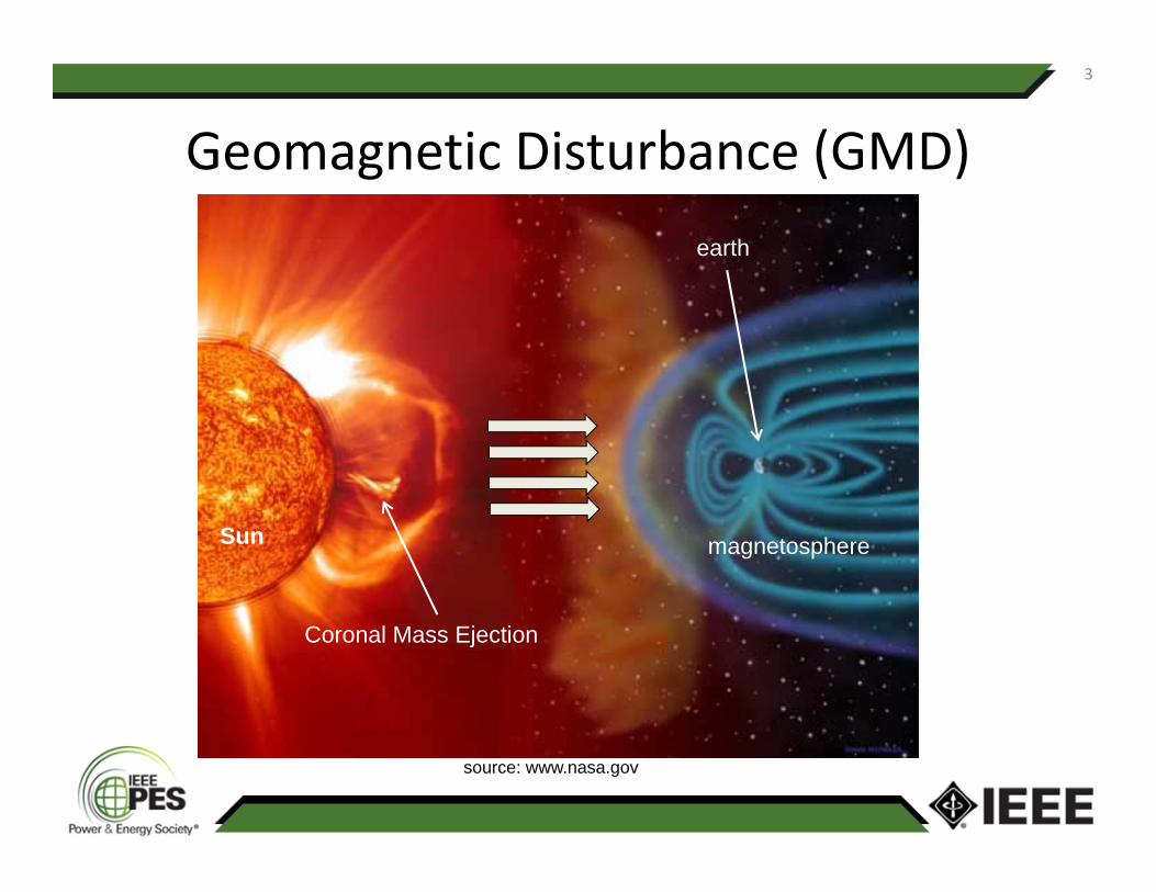
Geomagnetic Disturbance (GMD)3
source: www.nasa.gov
Coronal Mass Ejection
Sun
earth
magnetosphere
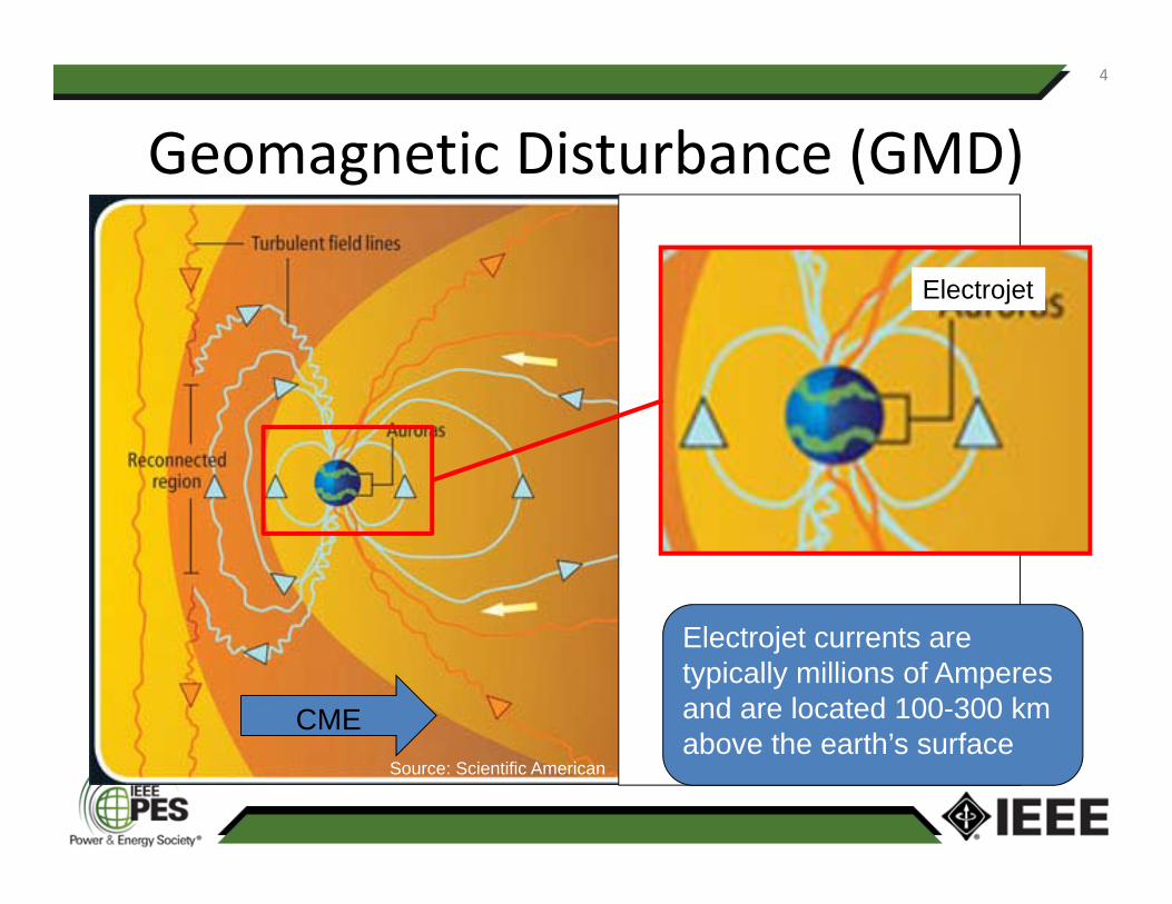
Geomagnetic Disturbance (GMD)4
Electrojet
Electrojet currents are typically millions of Amperes and are located 100-300 km above the earth’s surface
CMESource: Scientific American
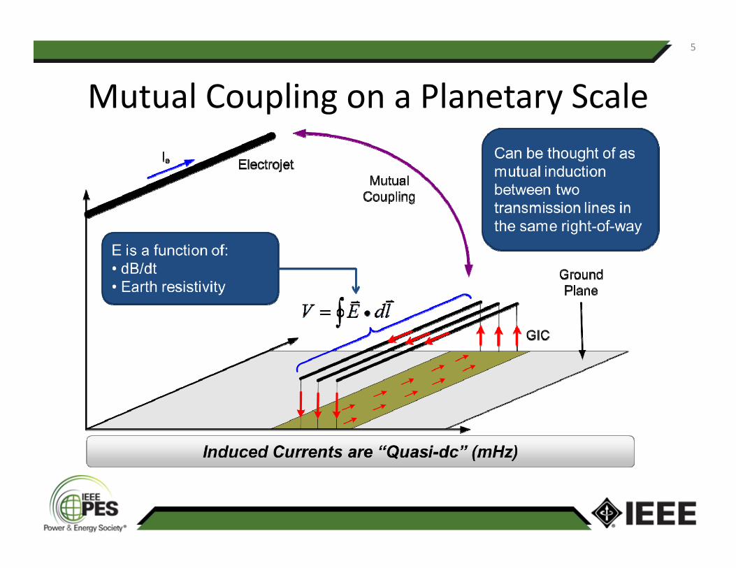
Mutual Coupling on a Planetary Scale5
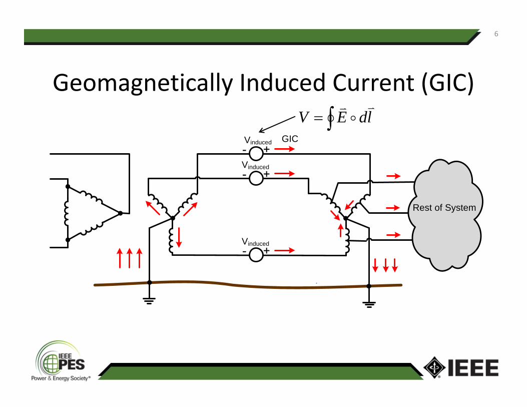
Geomagnetically Induced Current (GIC)
6
ldEV
Geoelectric Field
GICVinduced
Vinduced
Vinduced
Rest of System
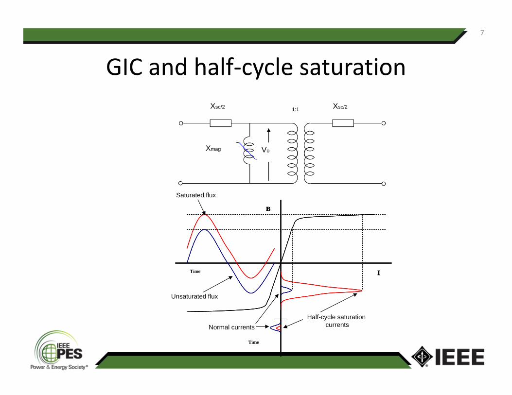
GIC and half‐cycle saturation7
Xsc/2
Xmag Vo
1:1 Xsc/2
Time I
B
Time
Time I
B
Time
Time I
B
Time
Unsaturated flux
Saturated flux
Normal currentsHalf-cycle saturation
currents

8
As saturation increases so does the magnitude and distortion of magnetizing currents
20 A
47 A
33 A
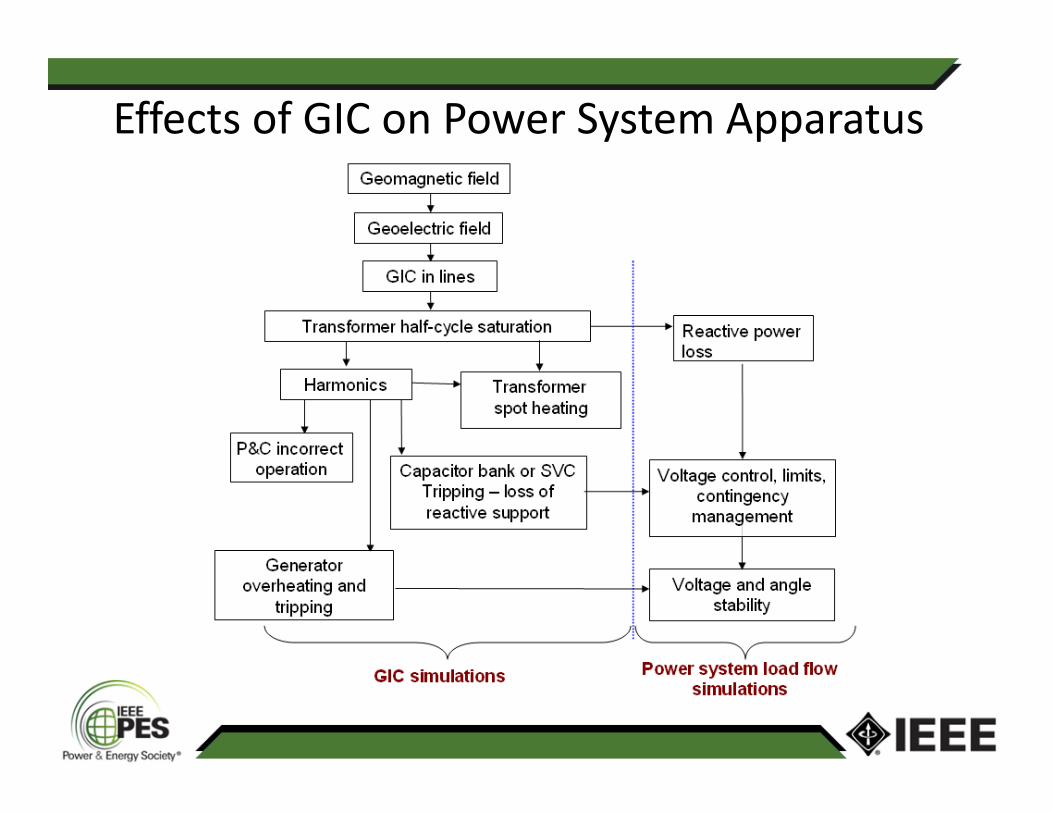
Effects of GIC on Power System Apparatus

• Magnetizing currents during half‐cycle saturation can be visualized as placing a small shunt reactive branch during half the 60 Hz cycle.
• The power system sees this as “effective” reactive power absorption
• This causes RMS voltages to drop• The time constant difference between GIC changes and the system response, allows the assumption that transformer reactive power absorption is nearly instantaneous and final steady‐state values for var loss can be modelled in a load flow program as a constant var source.
• Reactive power absorption assumes undistorted system voltages Q = V60 I60, where subscript 60 indicates the fundamental of voltage and current
Transformer reactive power absorption

Reactive power absorption and core type

ESSA GIC
-30
-20
-10
0
10
20
30
40
50
60
14:2
4
19:1
2
0:00
4:48
9:36
14:2
4
Time
ASpike at 22:44 July 26, 2004, EST
Neu
tral c
urre
nts
For instance…GMD event July 26‐27, 2004

526
528
530
532
534
536
538
20:5
2
21:2
1
21:5
0
22:1
9
22:4
8
23:1
6
23:4
5
0:14
Time
kV
CWDHNMBruce
500kV voltage responses July 26, 2004

243244245246247248249250251
21:2
1
21:3
6
21:5
0
22:0
4
22:1
9
22:3
3
22:4
8
23:0
2
23:1
6
23:3
1
23:4
5
0:00
Time
kV
ESSACLV
230kV voltage responses July 26, 2004
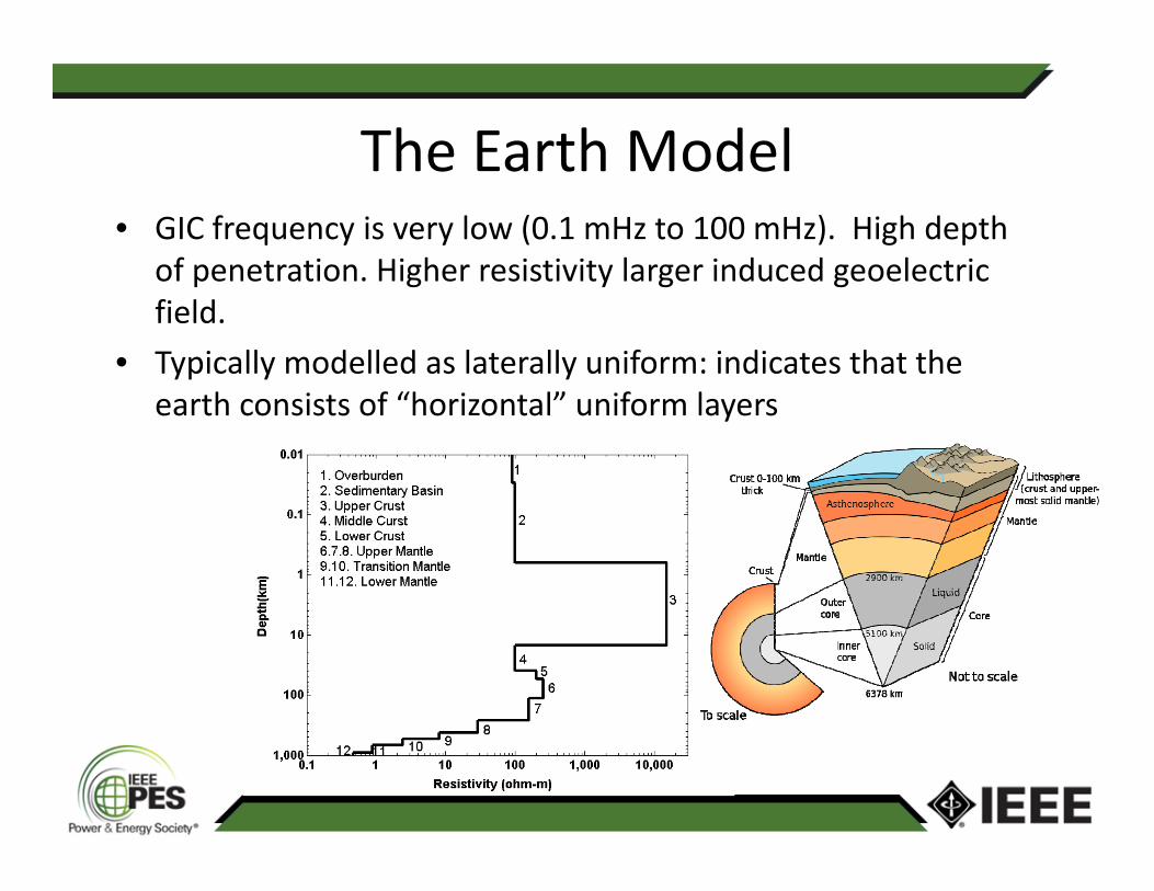
The Earth Model• GIC frequency is very low (0.1 mHz to 100 mHz). High depth
of penetration. Higher resistivity larger induced geoelectric field.
• Typically modelled as laterally uniform: indicates that the earth consists of “horizontal” uniform layers
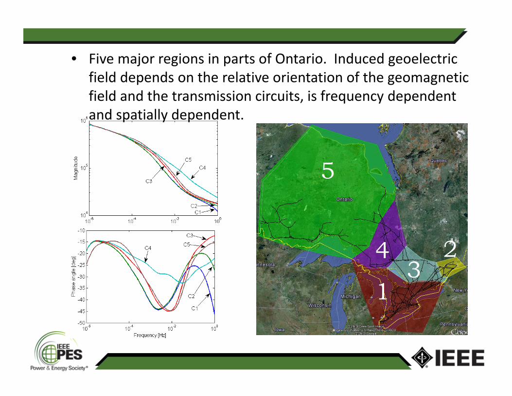
• Five major regions in parts of Ontario. Induced geoelectric field depends on the relative orientation of the geomagnetic field and the transmission circuits, is frequency dependent and spatially dependent.
Real‐time vs. Steady‐stateStudy purpose
• Real‐time– Situational awareness in the control room
– Alarms– Triggers for pre‐planned mitigation measures
– Event playback
• Steady‐state– Planning– Impact assessment– Determination of mitigating measures and their effectiveness

Real‐time vs. Steady‐stateGIC Modelling
• Real‐time– dc network – GIC and var absorption– E‐field from dB/dt
• Single or multiple earth models
– GIC and harmonics– GIC and transformer thermal response
• Steady‐state– dc network– GIC and var absorption– Usually uniform B‐field
• Different orientation• Single or multiple earth models
• Single frequency (0.1mHz – 100 mHz)

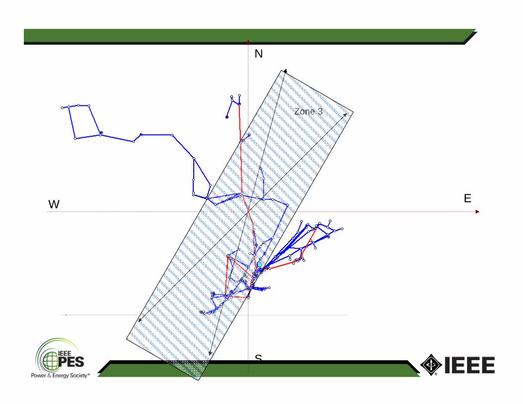
Storm orientation matters
EW
N
S
Zone 1

EW
N
S
Zone 2
EW
N
S
Zone 3

EW
N
S
Zone 4

EW
N
S
Zone 5

EW
N
S
Zone 6

• Probably since the early 1980’s for geophysical simulations. • NRCan’s real time GIC simulator was a GIC solver designed to provide a service to power system operators produced around the mid 2000’s. Focused on displaying GIC flows is a power network Graphical display Situational awareness.
• In the late 2000’s Hydro One’s real time simulator development started. Focused on real time assessment of var absorption and transformer hot spot heating. Arbitrary simulation time step (no FFT inversion)
In service in 2012.
GIC solvers

• The interface point between a GIC and a load flow simulation is transformer var absorption (assuming that netwotk topology is consistent)
• If GIC in every transformer is known for a given system configuration then the effects of var loss can be modelled in a load flow program by connecting a constant var source to the transformer terminals (constant I or constant Q).
Some commercial software do this transparently using lookup tables or var/GIC characteristics (or linear K‐factor) Different construction means a different lookup table or K‐factor Lookup tables are often obtained from published calculations but can also be generated with EMTP or equivalent simulations that take into consideration the distribution of flux according to construction.
Lookup tables always assume an infinite system source. In other words, harmonic currents do not cause harmonic voltage distortion.o Voltage/flux is assumed to be sinusoidal
Integration of GIC distribution and load flow

• Commercially available software that include GIC and load flow calculations is relatively young and evolving.
• Before GIC “modules/options” were available, integration was done with scripts running both applications: Calculate var absorption with GIC modeller Include var loss into load flow Obtain system voltage profile Iterate
Integration of GIC distribution and load flow

In a sense separate programs are a more powerful option since GIC simulators have more advanced features such as thermal transformer modelling, harmonics and complex earth models. In the case of 3‐limb core type transformers, the need to iterate between load flow and GIC solutions is important.
Integration of GIC distribution and load flow
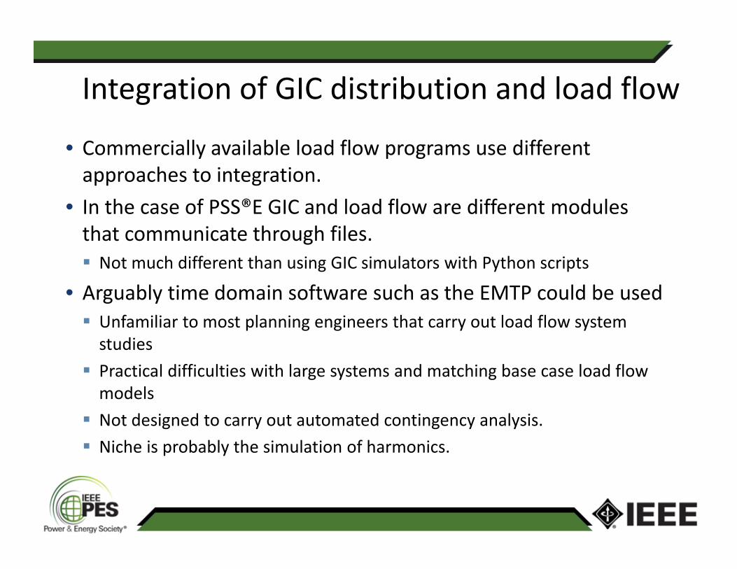
• Commercially available load flow programs use different approaches to integration.
• In the case of PSS®E GIC and load flow are different modules that communicate through files. Not much different than using GIC simulators with Python scripts
• Arguably time domain software such as the EMTP could be used Unfamiliar to most planning engineers that carry out load flow system studies
Practical difficulties with large systems and matching base case load flow models
Not designed to carry out automated contingency analysis. Niche is probably the simulation of harmonics.
Integration of GIC distribution and load flow

• Since circa 2010 when NERC’s GMD Task Force started, commercial software developers appreciated the need to account for GIC modelling in their tools.
• Complexities of GIC modelling are being introduced into commercial tools with varying approaches and simplifications. Different earth models Non‐uniform B‐field
• The “right way” to carry out system simulations is not quite there yet.
• Proposed NERC Standard TPL‐007 has been a powerful motivator.
Final observations