power quality and voltage stability of power systems with
TRANSCRIPT
University of Texas at TylerScholar Works at UT Tyler
Electrical Engineering Theses Electrical Engineering
Spring 4-30-2012
Power Quality and Voltage Stability of PowerSystems with a large share of Distributed EnergyResourcesYuva Nandan Reddy Chejerla
Follow this and additional works at: https://scholarworks.uttyler.edu/ee_grad
Part of the Electrical and Computer Engineering Commons
This Thesis is brought to you for free and open access by the ElectricalEngineering at Scholar Works at UT Tyler. It has been accepted forinclusion in Electrical Engineering Theses by an authorized administratorof Scholar Works at UT Tyler. For more information, please [email protected].
Recommended CitationChejerla, Yuva Nandan Reddy, "Power Quality and Voltage Stability of Power Systems with a large share of Distributed EnergyResources" (2012). Electrical Engineering Theses. Paper 7.http://hdl.handle.net/10950/66

POWER QUALITY AND VOLTAGE STABILITY OF POWER SYSTEMS
WITH A LARGE SHARE OF DISTRIBUTED ENERGY RESOURCES
by
YUVA NANDAN REDDY CHEJERLA
A thesis submitted in partial fulfillment
of the requirements for the degree of
Master of Science in Electrical Engineering
Department of Electrical Engineering
Hassan El-Kishky, Ph.D, P.E., Committee Chair
College of Engineering and Computer Science
The University of Texas at Tyler
May 2012


Acknowledgements
I am heartily thankful to my father Chejerla Lakshmana Reddy and mother Chejerla
Suneetha for their love, support, and encouragement in facing this challenge. My success
was dedicated to my brother Chejerla Sundeep Reddy, whom I love most and remember
throughout my life. I am grateful to my advisor Dr. Hassan El-Kishky for his
encouragement, patience, supervision and constant support from starting to the
concluding level. Without his guidance and help this thesis would not have been possible.
I would like to thank my committee members, Dr. Mukul Shirvaikar and Dr. Ron J.
Pieper for taking time and reviewing my work. I am grateful to the chair Dr. Mukul
Shirvaikar through whom I got admission to this university for my Master’s program and
also for supporting and guiding me throughout my Master’s program. I would like to
thank the entire EE department and the University of Texas at Tyler for supporting me
throughout my Master’s. Finally, I would like to thank all those, who supported me in
every aspect during the completion of the thesis.

i
Table of Contents
List of Figures .................................................................................................................................. iii
List of Tables .................................................................................................................................. vii
ABSTRACT ...................................................................................................................................... viii
CHAPTER ONE .................................................................................................................................. 1
1.1 Renewable Energy Sources in Power Systems ....................................................................... 1
1.2 Flexible AC Transmission Systems (FACTS) ............................................................................ 2
1.3 Literature Review ................................................................................................................... 2
1.4 Research Scope ...................................................................................................................... 3
1.5 Thesis Outline......................................................................................................................... 4
CHAPTER TWO ................................................................................................................................. 5
2.1 Overview ................................................................................................................................ 5
2.2 Wind Power............................................................................................................................ 5
2.2.1 Overview of Wind Power ................................................................................................ 6
2.2.2 Wind Turbine Speed Systems ......................................................................................... 8
2.2.3 Wind Power Integration .................................................................................................. 9
2.2.4 Wind Turbine Reactive Power Capability...................................................................... 10
2.3 Photovoltaic Systems ........................................................................................................... 10
2.3.1 Photovoltaic Performance ................................................................................................ 11
2.4 Fuel Cells .............................................................................................................................. 13
CHAPTER THREE ............................................................................................................................. 15
3.1 Introduction ......................................................................................................................... 15
3.2 Power System Specifications ............................................................................................... 15
3.3 Modeling and Control of a Power System ........................................................................... 17
3.3.1 Wind Farm Model ......................................................................................................... 17
3.4 Models of FACTS Controllers ............................................................................................... 19
3.4.1 Static Synchronous Compensator (STATCOM) ............................................................. 20
ii
3.4.2 Static VAR Compensator (SVC)...................................................................................... 22
3.4.3 Static Synchronous Series Compensator (SSSC) ........................................................... 24
3.4.4 Unified Power Flow Controller (UPFC) ......................................................................... 26
3.4.5 Comparison of STATCOM/SVC/SSSC/UPFC ................................................................... 28
CHAPTER 4 ..................................................................................................................................... 30
4.1 Power Quality of Power System .......................................................................................... 30
4.1.1 Steady Stage Voltage impact ........................................................................................ 31
4.1.2 Dynamic Voltage Variations .......................................................................................... 31
4.1.3 Harmonic Distortion ...................................................................................................... 31
4.2 Results and Discussion ......................................................................................................... 32
Role of FACTS Devices ................................................................................................................ 67
Voltage Stability ......................................................................................................................... 69
P-V Curves .............................................................................................................................. 70
Q-V Curves ............................................................................................................................. 71
Stability Curves .......................................................................................................................... 72
CHAPTER FIVE ................................................................................................................................ 78
Conclusions and Future Work .................................................................................................... 78
REFERENCES ................................................................................................................................... 80
iii
List of Figures
Figure 2.1: Basic parts of wind turbine 6
Figure 2.2: Power curve of wind turbine 8
Figure 2.3: Block diagram of double fed induction generator 9
Figure 2.4: Equivalent model of a PV cell 12
Figure 2.5: Characteristic of PV cell 12
Figure 2.6: Fuel cell schematic 13
Figure 2.7: Electrical characteristics of fuel cell 14
Figure 3.1: Simulation layout of a 12 Bus system 16
Figure 3.2: Internal model of wind turbine in MATLAB/Simulink 19
Figure 3.3: STATCOM and V-I Characteristics 20
Figure 3.4: STATCOM model in MATLAB/Simulink 21
Figure 3.5: SVC model and VI characteristics 23
Figure 3.6: SVC model in MATLAB/Simulink 23
Figure 3.7: SSSC stability model and power angle characteristics 25
Figure 3.8: SSSC model in MATLAB/Simulink 25
Figure 3.9: UPFC model and phasor representation of basic UPFC 27
Figure 3.10: UPFC model in MATLAB/Simulink 27
Figure 4.1: Without FACTS simulation results: Bus 2 voltage (top); Real power between
Bus 2 and Bus 3 (middle); Reactive power between Bus 2 and Bus 3 (bottom) 32
Figure 4.2: Without FACTS simulation results: Bus 3 voltage (top); Real power between
WF2 and Bus 3 (middle); Reactive power between WF2 and Bus 3 (bottom) 33
Figure 4.3: Without FACTS simulation results: Bus 4 voltage (top); Real power between
Bus4 and Bus 5 (middle); Reactive power between Bus 4 and Bus 5 (bottom) 34
Figure 4.4: Without FACTS simulation results: Bus 6 voltage (top); Real power between
WF1 and Bus 6 (middle); Reactive power between WF1 and Bus 6 (bottom) 35
iv
Figure4.5: Bus 4 voltage profile without FACTS 36
Figure 4.6: Bus 3 voltage profile without FACTS 36
Figure 4.7: Bus 4 voltage profile without FACTS 37
Figure 4.8: Bus 5 voltage profile without FACTS 37
Figure 4.9: Bus 6 voltage profile without FACTS 37
Figure 4.10: Bus 8 voltage profile without FACTS 38
Figure 4.11: Bus 11 voltage profile without FACTS 38
Figure 4.12: STATCOM device simulation results: Bus 2 voltage (top); Real power between
Bus 2 and Bus 3 (middle); Reactive power between Bus 2 and Bus 3 (bottom) 39
Figure 4.13: STATCOM device simulation results: Bus 3 voltage (top); Real power between
WF2 and Bus 3 (middle); Reactive power between WF2 and Bus 3 (bottom) 40
Figure 4.14: STATCOM device simulation results: Bus 4 voltage (top); Real power between
Bus4 and Bus 5 (middle); Reactive power between Bus 4 and Bus 5 (bottom) 41
Figure 4.15: STATCOM device simulation results: Bus 6 voltage (top); Real power between
WF1 and Bus 6 (middle); Reactive power between WF1 and Bus 6 (bottom) 42
Figure 4.16: Bus 2 voltage profile for a STATCOM simulation 43
Figure 4.17: Bus 3 voltage profile for a STATCOM simulation 44
Figure 4.18: Bus 4 voltage profile for a STATCOM simulation 44
Figure 4.19: Bus 5 voltage profile for a STATCOM simulation 44
Figure 4.20: Bus 6 voltage profile for a STATCOM simulation 45
Figure 4.21: Bus 8 voltage profile for a STATCOM simulation 45
Figure 4.22: Bus 11 voltage profile for a STATCOM simulation 45
Figure 4.23: SVC device simulation results: Bus 2 voltage (top); Real power between
Bus 2 and Bus 3 (middle); Reactive power between Bus 2 and Bus 3 (bottom) 46
Figure 4.24: SVC device simulation results: Bus 3 voltage (top); Real power between
WF2 and Bus 3 (middle); Reactive power between WF2 and Bus 3 (bottom) 47
Figure 4.25: SVC device simulation results: Bus 4 voltage (top); Real power between
Bus4 and Bus 5 (middle); Reactive power between Bus 4 and Bus 5 (bottom) 48
Figure 4.26: SVC device simulation results: Bus 6 voltage (top); Real power between
WF1 and Bus 6 (middle); Reactive power between WF1 and Bus 6 (bottom) 49

v
Figure 4.27: Bus 2 voltage profile for a SVC simulation 50
Figure 4.28: Bus 3 voltage profile for a SVC simulation 51
Figure 4.29: Bus 4 voltage profile for a SVC simulation 51
Figure 4.30: Bus 5 voltage profile for a SVC simulation 51
Figure 4.31: Bus 6 voltage profile for a SVC simulation 52
Figure 4.32: Bus 8 voltage profile for a SVC simulation 52
Figure 4.33: Bus 11 voltage profile for a SVC simulation 52
Figure 4.34: SSSC device simulation results: Bus 2 voltage (top); Real power between
Bus 2 and Bus 3 (middle); Reactive power between Bus 2 and Bus 3 (bottom) 53
Figure 4.35: SSSC device simulation results: Bus 3 voltage (top); Real power between
WF2 and Bus 3 (middle); Reactive power between WF2 and Bus 3 (bottom) 54
Figure 4.36: SSSC device simulation results: Bus 4 voltage (top); Real power between
Bus4 and Bus 5 (middle); Reactive power between Bus 4 and Bus 5 (bottom) 55
Figure 4.37: SSSC device simulation results: Bus 6 voltage (top); Real power between
WF1 and Bus 6 (middle); Reactive power between WF1 and Bus 6 (bottom) 56
Figure 4.38: Bus 2 voltage profile for a SSSC simulation 57
Figure 4.39: Bus 3 voltage profile for a SSSC simulation 58
Figure 4.40: Bus 4 voltage profile for a SSSC simulation 58
Figure 4.41: Bus 5 voltage profile for a SSSC simulation 58
Figure 4.42: Bus 6 voltage profile for a SSSC simulation 59
Figure 4.43: Bus 8 voltage profile for a SSSC simulation 59
Figure 4.44: Bus 11 voltage profile for a SSSC simulation 59
Figure 4.45: UPFC device simulation results: Bus 2 voltage (top); Real power between
Bus 2 and Bus 3 (middle); Reactive power between Bus 2 and Bus 3 (bottom) 60
Figure 4.46: UPFC device simulation results: Bus 3 voltage (top); Real power between
WF2 and Bus 3 (middle); Reactive power between WF2 and Bus 3 (bottom) 61
Figure 4.47: UPFC device simulation results: Bus 4 voltage (top); Real power between
Bus4 and Bus 5 (middle); Reactive power between Bus 4 and Bus 5 (bottom) 61
Figure 4.48: UPFC device simulation results: Bus 6 voltage (top); Real power between
WF1 and Bus 6 (middle); Reactive power between WF1 and Bus 6 (bottom) 63

vi
Figure 4.49: Bus 2 voltage profile for a UPFC simulation 64
Figure 4.50: Bus 3 voltage profile for a UPFC simulation 65
Figure 4.51: Bus 4 voltage profile for a UPFC simulation 65
Figure 4.52: Bus 5 voltage profile for a UPFC simulation 65
Figure 4.53: Bus 6 voltage profile for a UPFC simulation 66
Figure 4.54: Bus 8 voltage profile for a UPFC simulation 66
Figure 4.55: Bus 11 voltage profile for a UPFC simulation 66
Figure 4.56: P-V curve 71
Figure 4.57: V-Q curve 71
Figure 4.58: PV curve or nose curve for wind farm1 without FACTS 72
Figure 4.59: VQ curve for wind farm1 without FACTS 73
Figure 4.60: PV curve or nose curve for wind farm1 with STATCOM 73
Figure 4.61: VQ curve for wind farm1 with STATCOM 74
Figure 4.62: PV curve or nose curve for wind farm1 with SVC 74
Figure 4.63: VQ curve for wind farm1 with SVC 75
Figure 4.64: PV curve or nose curve for wind farm1 with SSSC 75
Figure 4.65: VQ curve for wind farm1 with SSSC 76
Figure 4.66: PV curve or nose curve for wind farm1 with UPFC 76
Figure 4.67: VQ curve for wind farm1 with UPFC 77
vii
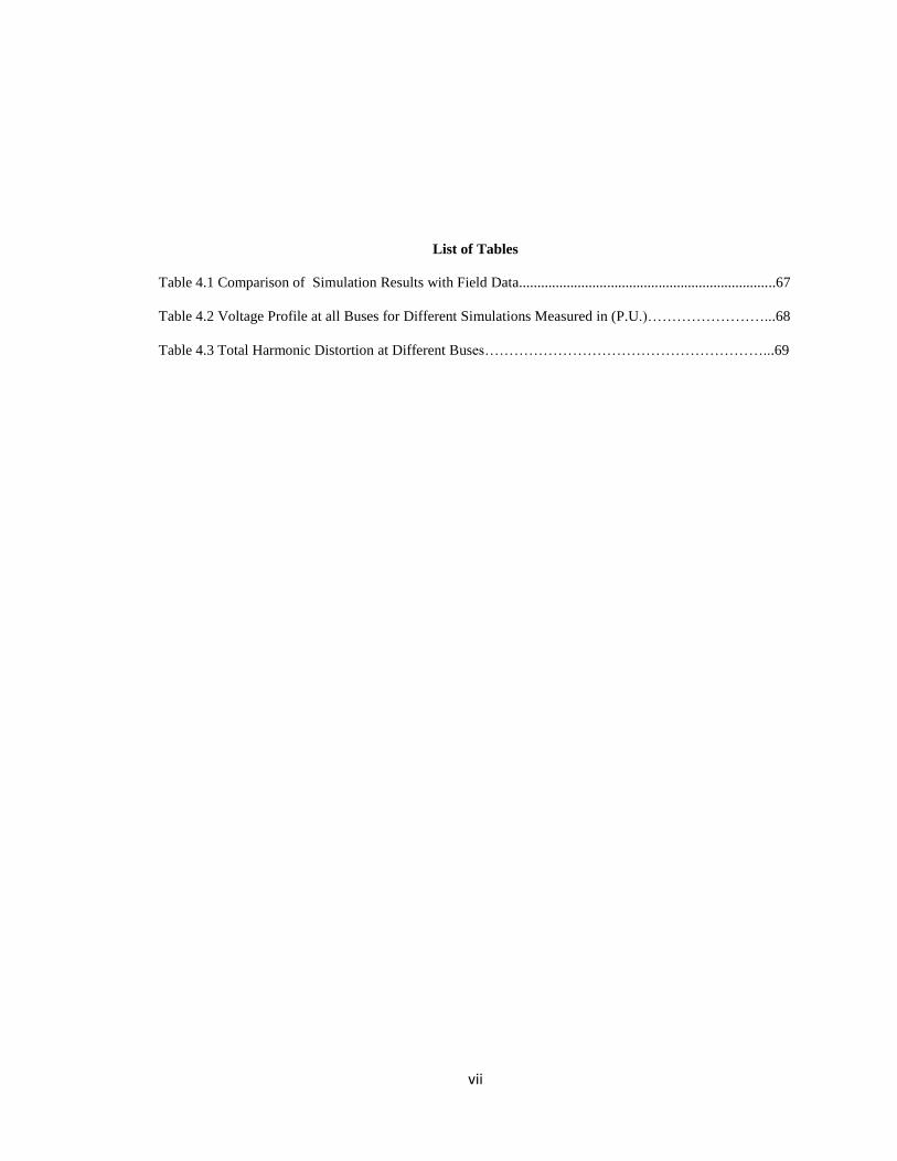
List of Tables
Table 4.1 Comparison of Simulation Results with Field Data......................................................................67
Table 4.2 Voltage Profile at all Buses for Different Simulations Measured in (P.U.)……………………...68
Table 4.3 Total Harmonic Distortion at Different Buses…………………………………………………...69

viii
Power Quality and Voltage Stability of Power Systems with a Large
Share of Distributed Energy Resources
Yuva Nandan Reddy Chejerla
Thesis Chair: Hassan El-Kishky, Ph.D, PE, MBA.
The University of Texas at Tyler
May 2012
ABSTRACT
The main objective of this research is to model and characterize power systems
with a large share of distributed energy resources. The effect of integrating distributed
energy resources such as wind farms, photovoltaic arrays, fuel cell stacks and micro-
hydroelectric generators on the power quality and voltage stability of power systems is
investigated and characterized. A comprehensive power system model was developed in
Matlab/Simulink environment. Stand-alone and grid-connected models of distributed
energy resources were developed and integrated into the system under investigation.
Several characteristics such bus voltage profiles, voltage transients, power flow, and total
harmonic distortion are captured and investigated. The integration of Flexible Alternating
Current Transmission Systems (FACTS) devices such as Static Synchronous Series
Compensator (SSST), Unified Power Flow Controller (UPFC), Static VAR Compensator
(SVC), and Static Compensator (STATCOM) into power systems was also studied.
Models of common FACTS devices were developed and integrated into the power system
model. The effect of installing FACTS devices on the power quality and voltage stability
of power systems with a significant component of distributed energy resources was
investigated. Power system characteristics with and without FACTS devices were
determined and investigated. From the simulation results, it is observed that there is a
ix
significant improvement in the power quality by integrating FACTS device. Future
research into the feasibility and optimal location of FACTS devices to improve power
system performance and operation will be needed.
1
CHAPTER ONE
Introduction
1.1 Renewable Energy Sources in Power Systems
The share of renewable energy resources in generating electricity has been
increasing in most parts of the world over the past few years [1]. Until the 18th
century
people got all of their energy from renewable sources such as wind, water, sun, and
wood. The use of fossil energy started during the 19th
century only because of
industrialization [2]. As of now, the world does not face any shortage of fossil energy,
but confirmed reserves of oil and coal will be depleted before the end of this century [1].
This has resulted in significant interest in renewable energy sources like solar energy,
wind power, biomass, etc. Difference in the amount of sunlight at various locations
causes wind currents that can be used to generate power. Also, solar energy indirectly
helps generate hydro power. Thus solar energy can either directly or indirectly be used
to generate power.
Power system performance depends on the control of voltage and frequency,
power quality and dynamic behavior of energy sources. It is technologically feasible to
generate electric power using renewable energy sources, however, the efficiency is low
when generating it in bulk quantities [2]. Moreover power quality is generally poor due
to extensive use of power electronics. More research is being performed to address the
issues of improving power quality and voltage stability with an increasing share of
power generation from renewable energy sources.

2
1.2 Flexible AC Transmission Systems (FACTS)
Power quality and voltage stability are major problems with modern power
systems. Flexible AC transmission (FACTS) technology has been introduced to address
these issues. FACTS technology helps in power control thereby enhancing the usable
capacity [3]. FACTS technology is a collection of controllers, which can be applied
either individually or in coordination with others to control the interrelated system
parameters that govern the operation of transmission systems [4]. FACTS devices such
as Static Compensator (STATCOM), Static VAR Compensator (SVC), Static
Synchronous Series Compensator (SSSC), and Unified Power Flow Controller (UPFC)
are used in order to solve the power quality and voltage stability issues to some extent.
1.3 Literature Review
The main aim of this research is to address and rectify power quality and voltage
problems in a power system with a large share of distributed energy resources.
Integration of Renewable energy sources (wind farms, photovoltaic cells, fuel cell, etc.)
into the power system has been under extensive research and development mostly
focusing on the issues like power quality and voltage stability of the system in [1-5].
The performance of different types of FACTS devices are compared between
and their characteristics have been studied extensively to understand their
implementation [6-11].
Power quality issues when distributed energy resources are connected to a
large system have also been studied [12-13]. When the renewable energy sources are
connected to a large system, power quality and voltage stability are significantly
affected. Due to their intermittent nature some studies on how FACTS devices help

3
improve power quality when installed near renewable energy resources have been
prepared [14-16]. Voltage stability is another important problem in literature [17-18].
The improvement of voltage stability by introducing FACTS devices near renewable
energy sources in a power system is a current area of interest [19-24].
In this study, a 12 Bus power system model was developed in
Matlab/Simulink using the Simpower systems module. The system is characterized and
power quality and voltage stability issues with and without FACTS devices are
simulated. Results show that power quality and voltage stability of power system can be
improved by using FACTS devices.
1.4 Research Scope
The aim of this research is to model and characterize power systems with a large
share of distributed energy resources. The effect of integrating distributed energy
resources such as wind farms, photovoltaic arrays, fuel cells, micro-hydroelectric
generators on the power quality and voltage stability of power systems has been
investigated and characterized. A comprehensive power system model has been
developed in the Matlab/Simulation environment. Stand-alone and grid-connected
simulink models of distributed energy resources were developed and integrated into the
system under investigation. Several characteristics such Bus voltage profiles, voltage
transients, power flow, and total harmonic distortion are captured and investigated. The
integration of FACTS devices such as SSSC, UPFC, SVC, and STATCOM into power
systems has also been studied. Simulink models of common FACTS devices were
developed and integrated into the power system model under research.

4
1.5 Thesis Outline
An outline of the thesis is as follows: Chapter two describes renewable energy
sources and their importance in power systems. Chapter three describes the modeling of
power systems and the study of FACTS devices in facilitating integration of large wind
farms in to a weak power system. Chapter Four describes the simulation results for
different models and discusses the performance of different FACTS models for solving
power quality and voltage stability issues. Chapter Five describes the conclusion and
discusses future work.
5
CHAPTER TWO
Renewable Energy Resources
2.1 Overview
The sun is the main source of energy with sunlight coming to earth in two
different ways: direct and diffused. Most solar energy systems utilize both direct and
diffused sunlight. Thus, the sun plays a major role both directly and indirectly in the
supply and generation of renewable energy. Renewable energy sources such as the sun,
wind and earth offer clean and abundant energy sources [2]. These resources are also
used to produce electricity for both domestic and industrial purposes. Approximately
10% of the energy consumed in the United States is from renewable sources with most
of the energy coming from hydro power, wind power, photovoltaic and biomass sources
[1]. Scientists and engineers are increasingly conducting more research on the
development of renewable energy sources. However there are major technical issues
facing the development and integration of renewable energy source such as power
quality and stability problems. The research work here is focused on modeling and
simulation of electric power systems with a large share of distributed energy sources
(DERs) and studies the impact on power quality and voltage stability with and without
flexible alternating current transmission system (FACTS) devices.
2.2 Wind Power
Wind energy is one of the most important renewable energy sources for the
generation of electrical power. The function of wind power systems is to convert kinetic
6
energy of the wind in to electric energy. In the past wind power was used primarily to
pump water as well as for grinding purposes. With the increase in oil prices, more
interest was shown in wind power as an alternative energy source. The focus shifted to
converting wind power to electric energy rather than mechanical energy. Electricity
generation from wind turbines has been advancing since the 1970s [2]. It has emerged as
the most sustainable energy source since the mid 1990s [2]. The cost of electricity from
wind power has fallen significantly due to intensive research and development.
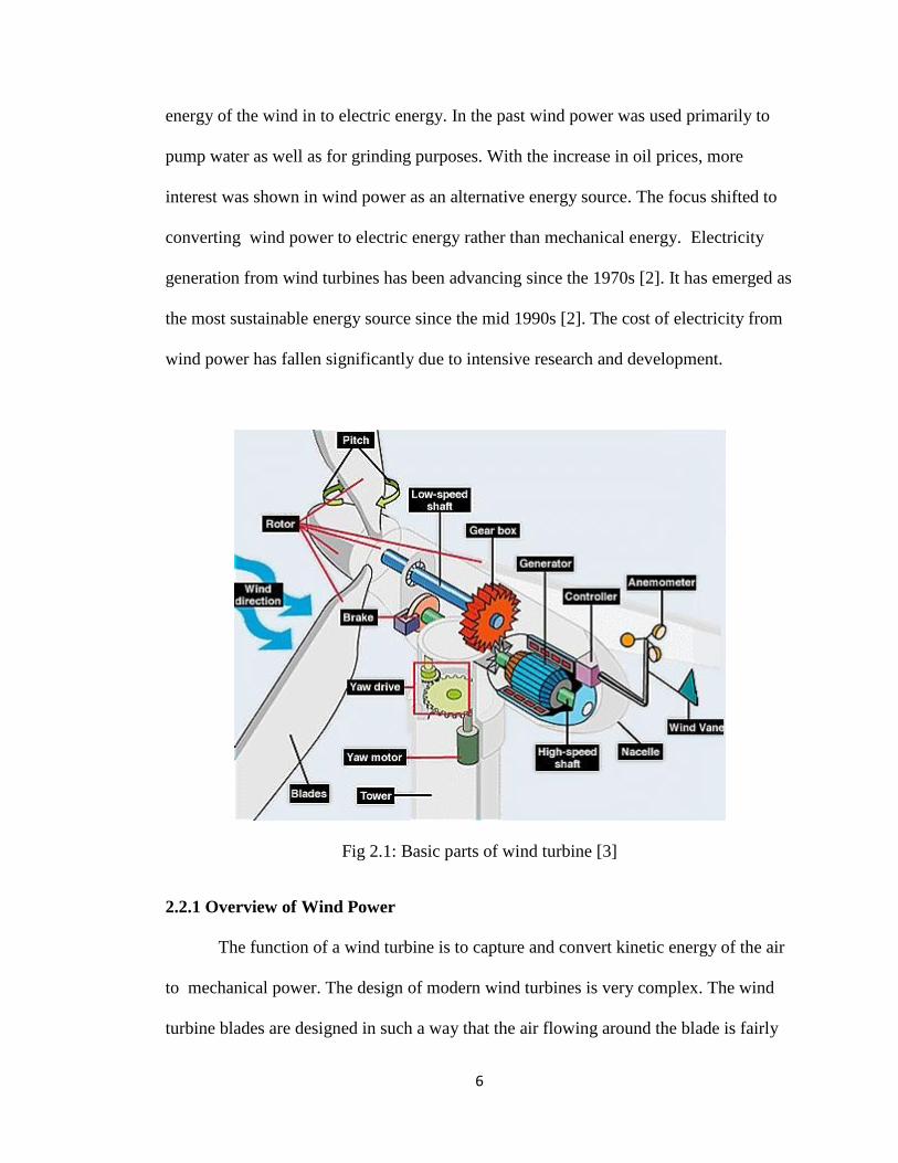
Fig 2.1: Basic parts of wind turbine [3]
2.2.1 Overview of Wind Power
The function of a wind turbine is to capture and convert kinetic energy of the air
to mechanical power. The design of modern wind turbines is very complex. The wind
turbine blades are designed in such a way that the air flowing around the blade is fairly

7
laminar up to an angle of attack of about 10 degrees. Major wind turbine components
include the rotor, the control unit, step up transformer, electrical generator, mechanical
transmission etc. The power of the wind (P) in a particular area is given by;
P=
) (2.1)
Where is the air density in (kg/ ), ‘A’ is area swept by the wind ( ), ‘ ’ is the
wind speed (m/s) [22].
The density of air can be calculated from the ideal gas equation as;
= p/( *T) (2.2)
Where p is absolute pressure in Pascal (pa), is the specific gas constant and T is
absolute temperature in Kelvin (K). The area (A) swept by the blade can be calculated as
the area of a circle formed by the rotation [22]. A small change in wind speed leads to
drastic changes in the power output. The average value of the wind speed is used to
calculate the output power.
Fig 2.2: Typical power curve of a wind turbine [3]

8
Normally, wind turbines are started when the wind speed exceeds 3-4 m/sec as
shown in Fig 2.2,which is called the cut-in speed. The rated output of a wind turbine is
capped at wind speeds from 12 to 25m/sec [3]. The wind turbine stops when the wind
speed exceeds 25m/sec which called the cutout speed to avoid excessive mechanical
forces.
2.2.2 Wind Turbine Speed Systems
There are two types of wind turbine speed systems namely fixed speed wind
turbines and variable speed wind turbines. The fixed speed wind turbines use induction
type generators and are equipped with capacitor bank for self excitation or rotor
resistance control in case of wound- rotor machines. These systems are widely used
because of their lower cost and higher mechanical compatibility under various wind
conditions. The generator along with the gear box are placed in a nacelle as shown in
Fig 2.1. Fixed speed wind turbines are especially designed to achieve maximum
efficiency at a single wind speed. Some fixed- speed wind turbines may have two
different rotational speeds in order to be able to capture more energy.
Variable-speed wind turbines are equipped with a converter which allows
generator frequency to differ from the grid frequency. Wind turbines operating within a
narrow speed range have a double fed induction generator with a converter which is
connected to the rotor circuit. Wind turbines operated within a broad variable-speed
range are furnished with a frequency converter. This converter makes it possible to use a
direct-driven generator which can operate at a very low speed and in this case a gear box
is not necessary. The advantages of variable-speed wind turbines over fixed speed

9
systems are power quality improvement, noise reduction and reduced mechanical stress
on the wind turbine
Fig 2.3: Block diagram of double fed induction generator [3]
2.2.3 Wind Power Integration
Integration of large amounts of wind power may lead to power quality and
voltage stability problems. In small-scale wind power integration, the installed wind
power is small compared to power system capacity [3]. In this type of integration only
voltage stability problems are of concern because frequency is kept constant and enough
spinning is normally reserved for active power. The active power from the wind turbine
is directly transferred to the power system without any storage devices. The disturbances
in the voltage can be classified as steady state and dynamic.
In large-scale wind power integration, the installed wind power is significant
compared to the power system capacity. In this type of integration both power quality
and voltage stability problems are of concern and in some cases frequency problems
arise. In large-scale wind power integration, a large wind farm is connected to the
transmission system or a large number of small wind turbines are connected to the

10
distribution system. In this type high wind power capacity is installed and active power
variations interact with frequency controllers in the power system which results in
variation in the system frequency. Both power quality and voltage stability of the system
mainly depend on the system controllability [3].
2.2.4 Wind Turbine Reactive Power Capability
The wind turbines coupled induction generators absorb reactive power from the
power system during normal operating conditions. Since wind turbines are considered a
sink for reactive power, an effective dynamic reactive power management system is
required to avoid voltage stability issues in the wind host power system. Under normal
operating conditions the double fed induction generators operate at close to unity power
factor and may supply some reactive power during system disturbances such as a three
phase fault close to the wind farm. Mechanically switched capacitors (MSCs) used in
wind farms contain asynchronous generators that are used to provide reactive power
support during system disturbances. However, MSCs are required to meet
interconnection standards such as to ride through a fault. Hence, additional
compensating equipment may be needed by the system in order to restore it quickly after
a fault has been cleared so as to maintain system stability and to avoid generator
tripping. In some instances, the collector Bus of the wind farm may have some reactive
power compensation, which is typically lower than that required for critical
contingencies in the system [3].
2.3 Photovoltaic Systems
The function of photovoltaics (PV) is to generate electric power from sunlight.
PVs are made of semiconductor materials such as silicon which convert sunlight to

11
electric power. These systems have a long life with little maintenance. Researchers are
currently focusing on developing more efficient semiconductor materials and designs to
expand power production. A new PV technology is emerging to generate electricity by
using the energy of heat and infrared radiation known as thermo photovoltaics, through
which power can be generated for longer periods of time. Photovoltaic systems can be
classified into two main systems namely stand-alone and grid-connected systems.
Stand-alone systems are cost-effective applications of photovoltaics that are mainly
used in the areas where it is not easy to connect to the grid. The difference between a
stand-alone system and a grid-connected system is that the solar energy output in
stand-alone systems is matched with load demand. These stand-alone systems are
comprised of solar modules, control units as well as storage elements and the loads.
Grid-connected photovoltaic systems help provide energy for both industrial and
household loads. The use of grid connected systems is fast increasing. There are
significant economical and technical issues when these systems are connected to the
power grids.
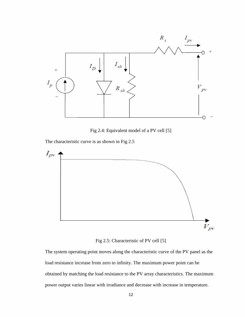
2.3.1 Photovoltaic Performance
The performance of a photovoltaic cells mainly depends on its characteristics and
efficiency. The equivalent circuit model of a photovoltaic cell is as shown in Fig 2.4.
The PV array consists of a number of individual PV cells that are connected together to
obtain a unit with a suitable power rating. The characteristic of the PV array can be
determined by multiplying the voltage of an individual cell by the number of cells
connected in series and multiplying the current by the number of cells connected in
parallel [5].
12
Fig 2.4: Equivalent model of a PV cell [5]
The characteristic curve is as shown in Fig 2.5
Fig 2.5: Characteristic of PV cell [5]
The system operating point moves along the characteristic curve of the PV panel as the
load resistance increase from zero to infinity. The maximum power point can be
obtained by matching the load resistance to the PV array characteristics. The maximum
power output varies linear with irradiance and decrease with increase in temperature.
13
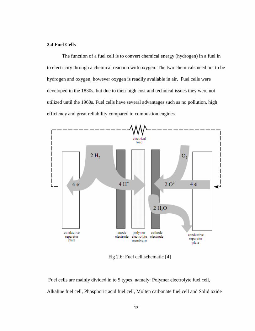
2.4 Fuel Cells
The function of a fuel cell is to convert chemical energy (hydrogen) in a fuel in
to electricity through a chemical reaction with oxygen. The two chemicals need not to be
hydrogen and oxygen, however oxygen is readily available in air. Fuel cells were
developed in the 1830s, but due to their high cost and technical issues they were not
utilized until the 1960s. Fuel cells have several advantages such as no pollution, high
efficiency and great reliability compared to combustion engines.
Fig 2.6: Fuel cell schematic [4]
Fuel cells are mainly divided in to 5 types, namely: Polymer electrolyte fuel cell,
Alkaline fuel cell, Phosphoric acid fuel cell, Molten carbonate fuel cell and Solid oxide

14
fuel cells. There are different types of fuel cell systems which include not only fuel cells
but also other components like pumps, fans, heaters, compressors, ejectors and a few
others [4]. The impact on the environment of fuel cell use depends upon the source of
the hydrogen used. Fuel cells emit fewer amounts of polluting gases for a given amount
of electricity when compared to conventional power generation.
In order to study the effect of fuel cells on power system performance a
mathematical model of the fuel cell has to be developed and integrated into the power
system under research [4]. To develop a mathematical model, the internal reaction of
the fuel cell has to be studied. A practical fuel cell has low efficiency when compared to
the ideal fuel cell due to losses in the cell reaction. The voltage drop from the open
circuit voltage is proportional to the current drawn by the circuit which is known as
polarization. Polarization can be classified as activation polarization, ohmic polarization
and concentrate polarization. Both ideal fuel cell and practical fuel cell characteristics
are shown in Figure 2.7 [4]. It is clear that the voltage drop is large at high current
outputs. From the electrical characteristic it is clear that concentration polarization is a
major cause of losses.
Fig 2.7: Electrical characteristics of a fuel cell [4]
15
CHAPTER THREE
Power System Modeling
3.1 Introduction
In this study a 12 Bus power system was modeled in the Matlab/Simulink
environment [12]. The model was developed using applicable physical principles and
experimental data. For power system simulation, a model has to be designed in such a
way that it has to obey all the input commands of different components of the system.
The simulation block diagram of the power system model is shown in Fig 3.1.
The model is evaluated and various simulation results such as Bus voltage profile
at different, active and reactive power at different Buses as well as PV and VQ curves
are generated.
3.2 Power System Specifications
The modeled system includes two wind farms (WFs) WF1 and WF2 which are
connected to the 69kV loop power system at Bus 6 and Bus 3 respectively. The loads
tapped on the weak loop system are 10 MW three phase dynamic loads. The system is
supplied by two main substations, which are represented by two remote boundary
equivalent sources at Buses 1 and 12. Among them, Bus 1 is the strong Bus with a short
circuit capacity of about 4000 MVA. The WF2 at Bus 3 is a large wind farm with a total
rating of 100 MVA. The WF1 at Bus 6 is located at the middle of weak 69 kV sub
transmission system and the short circuit capacity at Bus 5 is about 152 MVA. The

16
Fig
3.1
: S
imula
tion l
ayout
of
the
12 b
us
syst
em

17
integration of WF2 into the grid is facilitated by the power converter based interface as
it provides VAR compensation capability and, hence, voltage control capability. Thus,
when WF1 is connected at the weakest part of the loop system, these characteristics of
WF1 not only increases the transmission and distribution losses, reduces the system
voltage stability margin and limits power generation, but also causes severe voltage
fluctuations which may irritate the customers on the system, particularly in the weak
69kV loop, where a significant portion of the loads are induction motors, which are
sensitive to voltage fluctuations. Small size mechanical switched capacitors (MSCs) are
installed at each individual squirrel cage induction generator terminal (SCIG) and large
size MSCs (1~2 MVAR) are installed at Bus 6, the 35 kV secondary side of the WF1
main transformer T3 to reduce the voltage fluctuations and improve power quality. All
the main transformers T1 - T4 are equipped with electronic tap changers to provide
voltage support.
3.3 Modeling and Control of a Power System
Only positive sequence dynamic models developed in this study with only
balanced operation are considered. Loads are considered as constant power.
Transformer models are developed using MATLAB/Simulink transformer modeling
tools. The boundary equivalent voltage source is modeled using ideal voltage sources
with series equivalent impedances.
3.3.1 Wind Farm Model
When a large number of wind turbines are added to the system, the grid becomes
weaker as these types of generators require additional equipment as they do not have self
recovery capability. There exist standard specifications requirements for both normal

18
and dynamic performance of a wind turbine during disturbance. A large wind farm is
normally considered as comprised of a large number of smaller wind turbines. It is
difficult to represent all individual wind turbines practically in a power system to
perform a simulation study. The assumptions made to develop wind farm models are as
follow: (1) all wind turbines are identical, (2) wind speed are uniform, (3) each turbine
runs in the same operating mode at all times,(4) the voltages, current and power factor
of each turbine are the same; With these assumptions, both WF1 and WF2 are developed
as quasi-dynamic models so that all real power, reactive power and voltage of wind
farms are dynamically controlled. The model allows for recurring system operation from
the data of a steady state operating point study and continues for dynamic study. The
real power of WF is controlled by the source phase angle, the reactive power is
controlled by a shunt cap bank at the 35kV Bus of WFs, and the Bus voltage of WF is
controlled by the source voltage. The Wind turbine model developed in
By tuning the boundary sources, WFs and the non-monitored loads, this
operating point is simulated. Therefore, the 12-Bus system model with WFs at the
specific operating point is validated. Simulation result and field data at an operating
point compared. The simulated real power, reactive power and voltage follow almost the
same fluctuation trend and magnitude, and also have good match in terms of the steady-
state values.
The MATLAB/Simulink of a double-fed induction generator wind turbineis
shown in Fig 3.2.

19
Fig 3.2: Internal model of wind turbine in MATLAB/Simulink
3.4 Models of FACTS Controllers
The main functions of the FACTS devices used in power systems are to control
power flow, increase transmission capability, provide transient voltage support to
prevent system collapse and power oscillation damping. FACTS devices installed in
wind power systems are used to improve the transient as well as dynamic stability of the
overall power system. Four types of FACTS devices are chosen in this study by
considering all the above requirements. A brief description of each of the FACTS
devices and their capabilities is given below.
20
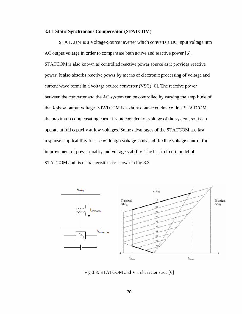
3.4.1 Static Synchronous Compensator (STATCOM)
STATCOM is a Voltage-Source inverter which converts a DC input voltage into
AC output voltage in order to compensate both active and reactive power [6].
STATCOM is also known as controlled reactive power source as it provides reactive
power. It also absorbs reactive power by means of electronic processing of voltage and
current wave forms in a voltage source converter (VSC) [6]. The reactive power
between the converter and the AC system can be controlled by varying the amplitude of
the 3-phase output voltage. STATCOM is a shunt connected device. In a STATCOM,
the maximum compensating current is independent of voltage of the system, so it can
operate at full capacity at low voltages. Some advantages of the STATCOM are fast
response, applicability for use with high voltage loads and flexible voltage control for
improvement of power quality and voltage stability. The basic circuit model of
STATCOM and its characteristics are shown in Fig 3.3.
Fig 3.3: STATCOM and V-I characteristics [6]

21
The STATCOM model in MATLAB/Simulink is shown in Fig 3.5
Fig 3.4: STATCOM model in MATLAB/Simulink
The STATCOM model is designed using Insulated gate Bipolar Transistor (IGBT)
based pulse width modulation VSC. From the Matlab model it is observed that during
simulation, the STATCOM control system keeps the fundamental component of the
VSC voltage in phase with the system voltage. The STATCOM generates reactive
power only if the voltage generated by the VSC is higher than the system voltage. The
amount of reactive power depends on the transformer leakage reactance. The function of
the control system is to increase or decrease the capacitor DC voltage, so that the
generated AC voltage has the correct amplitude for the required reactive power.
22
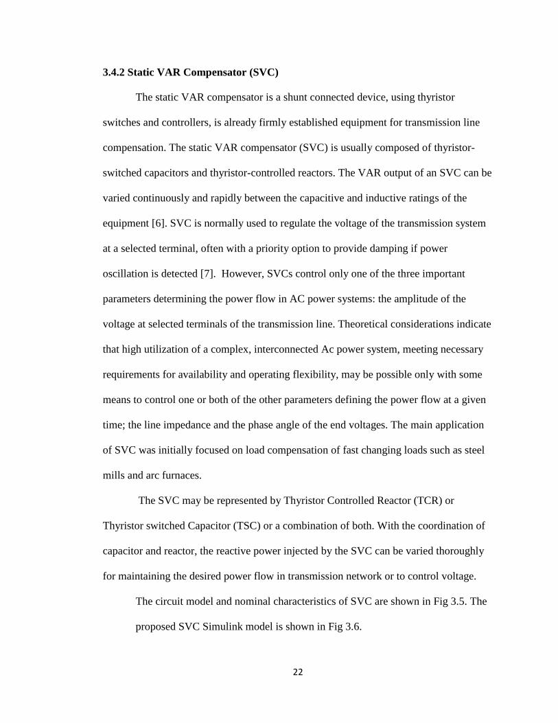
3.4.2 Static VAR Compensator (SVC)
The static VAR compensator is a shunt connected device, using thyristor
switches and controllers, is already firmly established equipment for transmission line
compensation. The static VAR compensator (SVC) is usually composed of thyristor-
switched capacitors and thyristor-controlled reactors. The VAR output of an SVC can be
varied continuously and rapidly between the capacitive and inductive ratings of the
equipment [6]. SVC is normally used to regulate the voltage of the transmission system
at a selected terminal, often with a priority option to provide damping if power
oscillation is detected [7]. However, SVCs control only one of the three important
parameters determining the power flow in AC power systems: the amplitude of the
voltage at selected terminals of the transmission line. Theoretical considerations indicate
that high utilization of a complex, interconnected Ac power system, meeting necessary
requirements for availability and operating flexibility, may be possible only with some
means to control one or both of the other parameters defining the power flow at a given
time; the line impedance and the phase angle of the end voltages. The main application
of SVC was initially focused on load compensation of fast changing loads such as steel
mills and arc furnaces.
The SVC may be represented by Thyristor Controlled Reactor (TCR) or
Thyristor switched Capacitor (TSC) or a combination of both. With the coordination of
capacitor and reactor, the reactive power injected by the SVC can be varied thoroughly
for maintaining the desired power flow in transmission network or to control voltage.
The circuit model and nominal characteristics of SVC are shown in Fig 3.5. The
proposed SVC Simulink model is shown in Fig 3.6.
23
Fig 3.5: SVC model and VI characteristics [6]
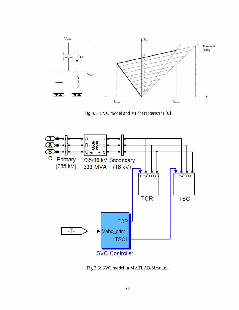
Fig 3.6: SVC model in MATLAB/Simulink
24
From the Matlab model it is observed that TCR and TSC are connected to the secondary
side of the transformer. Switching the TSCs in and out allows a discrete variation of the
secondary reactive power. The function of the SVC controller is to monitor the primary
voltage and sends appropriate pulses to the thyristors in order to obtain the susceptance
required by the voltage regulator. SVC generates reactive power when the system
voltage is low when compared to SVC capacitive voltage and absorbs reactive power
when system voltage is higher than SVC capacitive voltage.
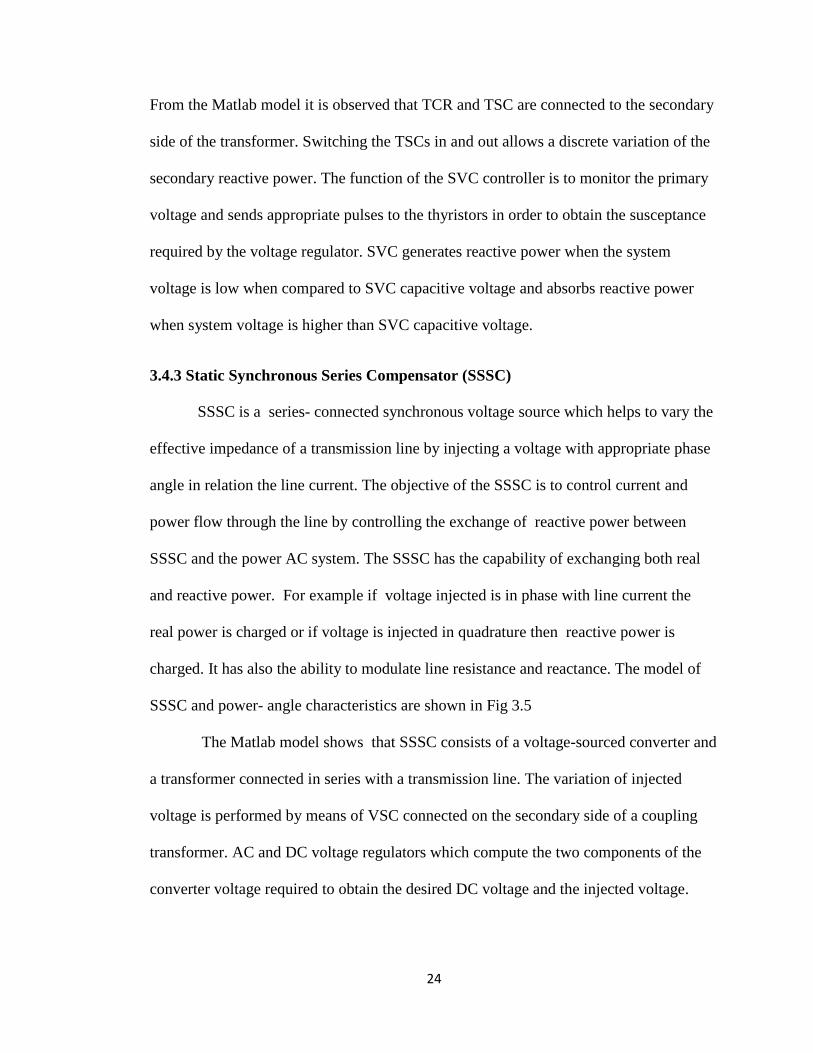
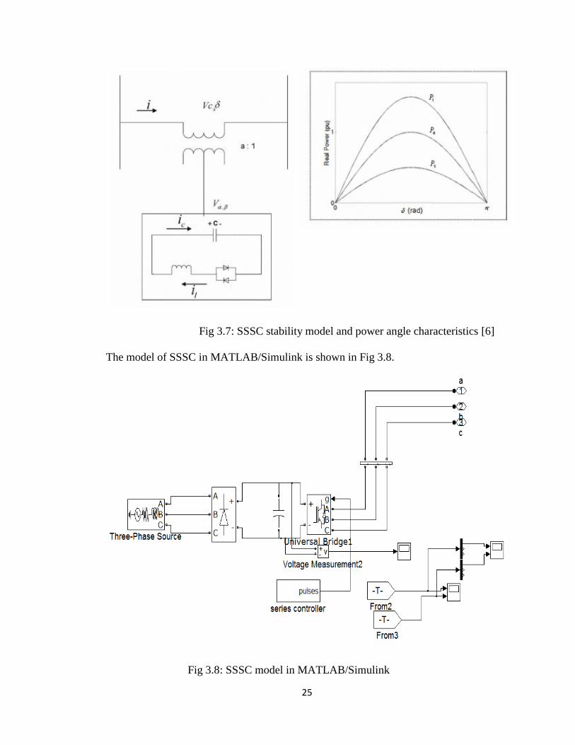
3.4.3 Static Synchronous Series Compensator (SSSC)
SSSC is a series- connected synchronous voltage source which helps to vary the
effective impedance of a transmission line by injecting a voltage with appropriate phase
angle in relation the line current. The objective of the SSSC is to control current and
power flow through the line by controlling the exchange of reactive power between
SSSC and the power AC system. The SSSC has the capability of exchanging both real
and reactive power. For example if voltage injected is in phase with line current the
real power is charged or if voltage is injected in quadrature then reactive power is
charged. It has also the ability to modulate line resistance and reactance. The model of
SSSC and power- angle characteristics are shown in Fig 3.5
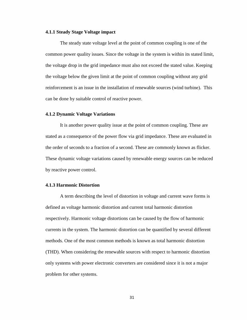
The Matlab model shows that SSSC consists of a voltage-sourced converter and
a transformer connected in series with a transmission line. The variation of injected
voltage is performed by means of VSC connected on the secondary side of a coupling
transformer. AC and DC voltage regulators which compute the two components of the
converter voltage required to obtain the desired DC voltage and the injected voltage.
25
Fig 3.7: SSSC stability model and power angle characteristics [6]
The model of SSSC in MATLAB/Simulink is shown in Fig 3.8.
Fig 3.8: SSSC model in MATLAB/Simulink

26
3.4.4 Unified Power Flow Controller (UPFC)
Power flow in an AC transmission system is a function of transmission line
impedance, the magnitude of the sending end and receiving end voltages and the phase
angle between these voltages [3]. The objective of the unified power flow controller
(UPFC) is to control (regulate), concurrently or selectively all these parameters [5]. The
concept of UPFC broadens the basic power transmission concepts. It allows not only the
combined application of phase angle control with controllable series and shunt reactive
compensation, but also the real-time transition from one selected compensation mode
into another one to handle particular system contingencies more effectively (for example,
series reactive compensation could be replaced by phase angle control or vice versa).
This may become especially important in complex transmission systems where control
compatibility and coordination of various FACTS devices must be maintained in case of
equipment failure and system changes [6]. This concept would also provide considerable
operating flexibility by its inherent adaptability to power system expansions and changes
without any hardware alterations. UPFC is widely considered the most versatile
controller having all the capabilities of voltage regulation, series compensation and phase
shifting. The real and reactive power flow can be controlled independently. It has both
shunt and series converters which are connected by DC link. The series converter is
controlled to inject the voltage in series with the line. This converter can exchange both
real and reactive power with the transmission line. The shunt connected converter is used
to supply the real power demand to the series converter. The UPFC model circuit
diagram and Simulink are shown in Figures 3.9 and 3.10 respectively.

27
Fig3.9: UPFC model and phasor representation of basic UPFC [6]
The model of UPFC in MATLAB/Simulink is shown in Fig 3.10.
Fig 3.10: UPFC model in MATLAB/Simulink

28
From the UPFC Matlab model it is observed that shunt and series converters are
connected by a DC link. The UPFC is a combination of STATCOM and SSSC. It
performs the function of both devices. Shunt converter operating as a STATCOM
controls voltage and Series converter operating as a SSSC controls injected voltage,
while keeping injected voltage in quadrature with current.
3.4.5 Comparison of STATCOM/SVC/SSSC/UPFC
FACTS devices have shown strong influence on system stability and less impact
on power quality. However, STATCOM and SVC have a strong influence on voltage
quality and system stability as well. The SSSC has strong influence on system stability,
however its performance for maintaining voltage quality is average. The UPFC has
efficient performance in all terms like stability, voltage quality and power contingency
support. In this research the main objective is to provide solutions to power quality and
voltage stability problems in systems with large share of DERs. STATCOM and SVC are
shunt connected reactive power compensation devices that are capable of absorbing and
generating reactive power. From the VI characteristics it is clear that the STATCOM has
more reactive power control than SVC. The maximum compensating current of the SVC
decreases linearly with the AC system voltage and the maximum VAR output decreases
with the square of the voltage. By comparing these two it is clear that for the same
dynamic performance of the system, a higher SVC rating than that of STATCOM would
be required. The main objective of the UPFC is to be able to control both active and
reactive power in the power system. When compared to the UPFC and SSSC they are not
very economical and also involve complicated control techniques. They also occupy

29
more space when compared with STATCOM or SVC. Mechanically switched capacitors
do not perform well at low voltages.
The location for placing the FACTS device in a power system model is another
important factor that plays a crucial role in the operation and control of a power system
with high power quality and voltage stability. The best location for the FACTS device is
near the weakest Bus of the system for better voltage stability and power quality. The
weakest Bus is identified as the Bus where the first voltage collapse occurance is
identified. In this research Bus 6 is considered as the weakest Bus i.e. near the wind farm
1. Thus FACTS devices are installed near Bus 6 and wind farm1 in order to obtain better
results.

30
CHAPTER 4
Simulation and Results
4.1 Power Quality of Power System
Different types of issues are to be considered in order to deal with power quality.
If a device is connected to electric grid, then that device has to fulfill all standard power
quality requirements. The issues dealing with power quality are static voltage level,
voltage fluctuations, voltage transients, voltage harmonic distortion, power supply
interruptions. The distributed energy stations are likely to violate some power quality
limits when they are improperly chosen for particular grid conditions. Some of the
power quality issues are discussed in the following sections.
A renewable energy source is designed to supply active power to the grid.
Reactive power exchange between the grid and a renewable energy source depends on
whether it can be consumed or produced. Increase in production of active power is
followed by an increase in the voltage drop over grid resistance and a consequent
increase at the point of common coupling. Power quality evaluation of renewable
energy sources are observed under two different operational modes. First, it is to be
observed under normal conditions such as steady state voltage impact, dynamic voltage
variations etc. Second, the impact on the grid when the renewable sources are connected
i.e. during the start up of device (wind turbine). Voltage transients originating in the
switching of a capacitor bank is another power quality problem.
31
4.1.1 Steady Stage Voltage impact
The steady state voltage level at the point of common coupling is one of the
common power quality issues. Since the voltage in the system is within its stated limit,
the voltage drop in the grid impedance must also not exceed the stated value. Keeping
the voltage below the given limit at the point of common coupling without any grid
reinforcement is an issue in the installation of renewable sources (wind turbine). This
can be done by suitable control of reactive power.
4.1.2 Dynamic Voltage Variations
It is another power quality issue at the point of common coupling. These are
stated as a consequence of the power flow via grid impedance. These are evaluated in
the order of seconds to a fraction of a second. These are commonly known as flicker.
These dynamic voltage variations caused by renewable energy sources can be reduced
by reactive power control.
4.1.3 Harmonic Distortion
A term describing the level of distortion in voltage and current wave forms is
defined as voltage harmonic distortion and current total harmonic distortion
respectively. Harmonic voltage distortions can be caused by the flow of harmonic
currents in the system. The harmonic distortion can be quantified by several different
methods. One of the most common methods is known as total harmonic distortion
(THD). When considering the renewable sources with respect to harmonic distortion
only systems with power electronic converters are considered since it is not a major
problem for other systems.
32
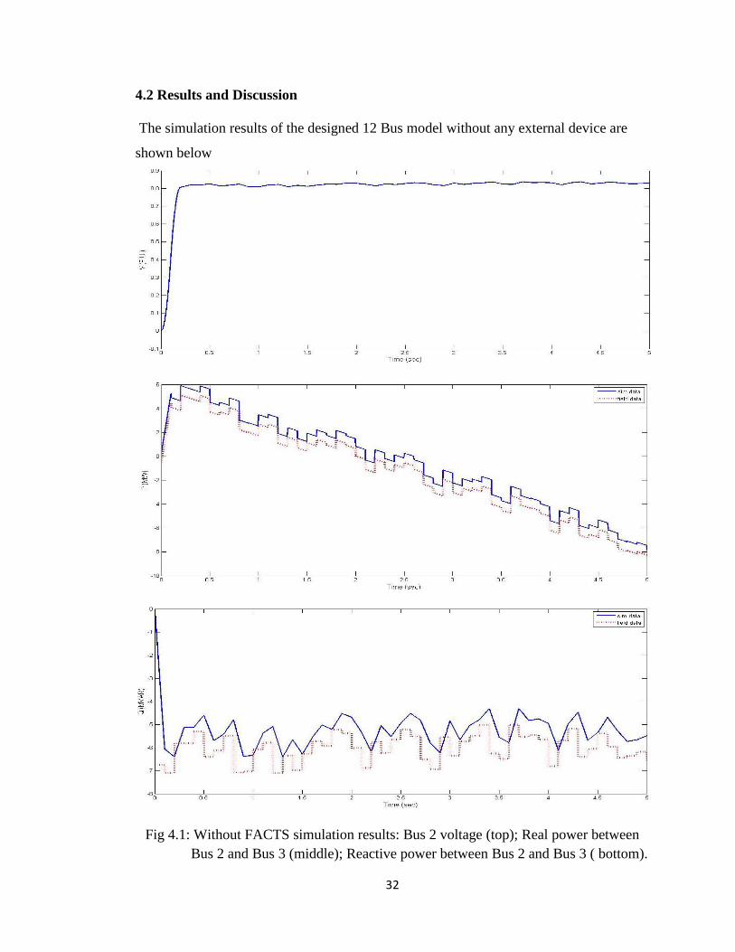
4.2 Results and Discussion
The simulation results of the designed 12 Bus model without any external device are
shown below
Fig 4.1: Without FACTS simulation results: Bus 2 voltage (top); Real power between
Bus 2 and Bus 3 (middle); Reactive power between Bus 2 and Bus 3 ( bottom).

33
Fig 4.2: Without FACTS simulation results: Bus 3 voltage (top); Real power between
WF2 and Bus 3 (middle); Reactive power between WF2 and Bus 3 (bottom).
34
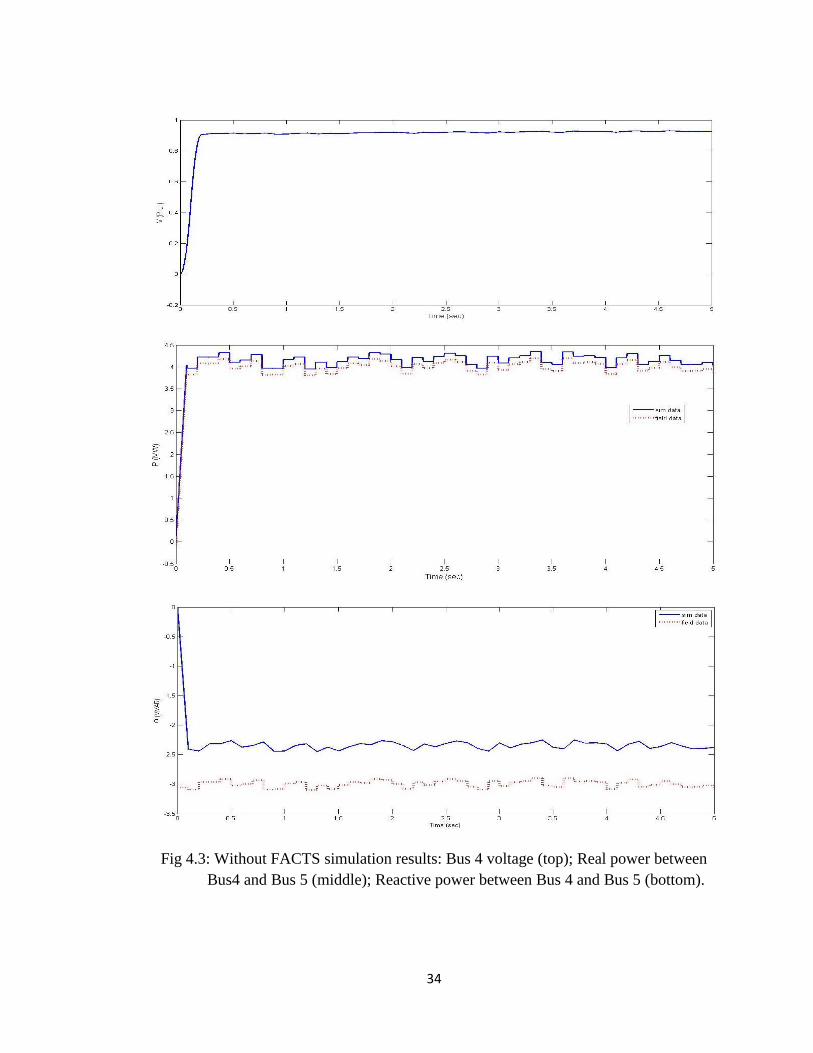
Fig 4.3: Without FACTS simulation results: Bus 4 voltage (top); Real power between
Bus4 and Bus 5 (middle); Reactive power between Bus 4 and Bus 5 (bottom).

35
Fig 4.4: Without FACTS simulation results: Bus 6 voltage (top); Real power between
WF1 and Bus 6 (middle); Reactive power between WF1 and Bus 6 (bottom).
36
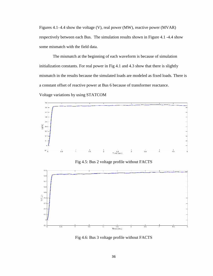
Figures 4.1–4.4 show the voltage (V), real power (MW), reactive power (MVAR)
respectively between each Bus. The simulation results shown in Figure 4.1 -4.4 show
some mismatch with the field data.
The mismatch at the beginning of each waveform is because of simulation
initialization constants. For real power in Fig 4.1 and 4.3 show that there is slightly
mismatch in the results because the simulated loads are modeled as fixed loads. There is
a constant offset of reactive power at Bus 6 because of transformer reactance.
Voltage variations by using STATCOM
Fig 4.5: Bus 2 voltage profile without FACTS
Fig 4.6: Bus 3 voltage profile without FACTS

37
Fig 4.7: Bus 4 voltage profile without FACTS
Fig 4.8: Bus 5 voltage profile without FACTS
Fig 4.9: Bus 6 voltage profile without FACTS
38
Fig 4.10: Bus 8 voltage profile without FACTS
Fig 4.11: Bus 11 voltage profile without FACTS
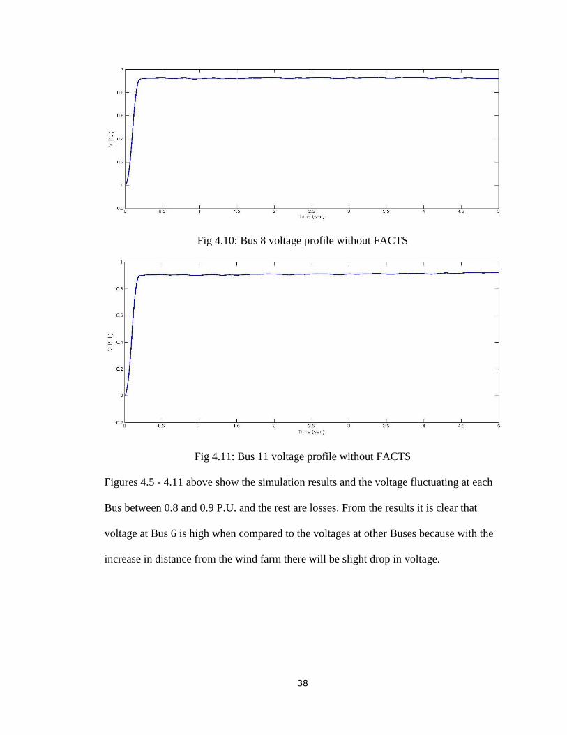
Figures 4.5 - 4.11 above show the simulation results and the voltage fluctuating at each
Bus between 0.8 and 0.9 P.U. and the rest are losses. From the results it is clear that
voltage at Bus 6 is high when compared to the voltages at other Buses because with the
increase in distance from the wind farm there will be slight drop in voltage.
39
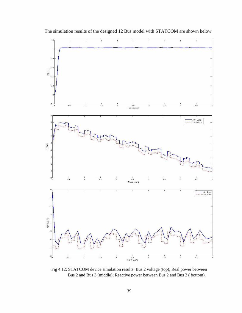
The simulation results of the designed 12 Bus model with STATCOM are shown below
Fig 4.12: STATCOM device simulation results: Bus 2 voltage (top); Real power between
Bus 2 and Bus 3 (middle); Reactive power between Bus 2 and Bus 3 ( bottom).

40
Fig 4.13: STATCOM device simulation results: Bus 3 voltage (top); Real power between
WF2 and Bus 3 (middle); Reactive power between WF2 and Bus 3 ( bottom).
41
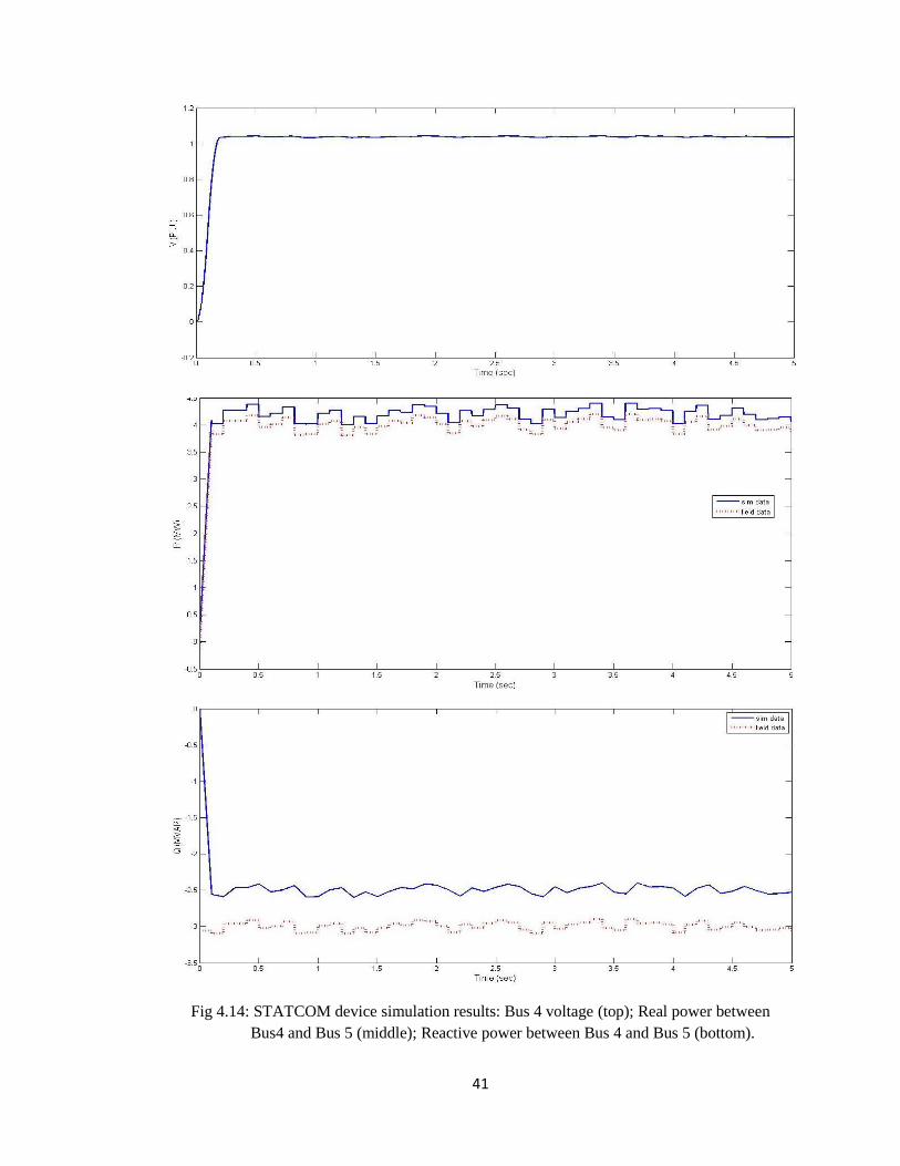
Fig 4.14: STATCOM device simulation results: Bus 4 voltage (top); Real power between
Bus4 and Bus 5 (middle); Reactive power between Bus 4 and Bus 5 (bottom).

42
Fig 4.15: STATCOM device simulation results: Bus 6 voltage (top); Real power between
WF1 and Bus 6 (middle); Reactive power between WF1 and Bus 6 (bottom).

43
Figures 4.12-4.15 shows the voltage (V), real power (MW), reactive power (MVAR)
respectively between each Bus. The simulation results shown in Fig 4.12-4.15 show
some mismatch with the field data.
The mismatch at the beginning of each waveform is because of the simulation
initialization constant. Fig 4.12 and Fig 4.14 for real power shows that there is slightly
mismatch in the results because the simulated loads are modeled as fixed loads. Because
of transformer reactance there is a constant offset of reactive power at Bus 6. There is a
constant increase in real power in figure 4.15 between Bus 3 and wind farm 2 when
compared with figure 4.2 i.e. without any FACTS device. From figure 4.15 there is an
increase in real power and drops to 0 due to load impact and increases at 4 seconds.
Voltage Variations
Fig 4.16: Bus 2 voltage profile for a STATCOM simulation
44
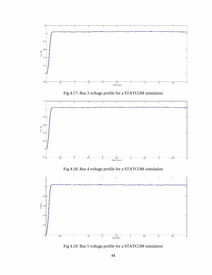
Fig 4.17: Bus 3 voltage profile for a STATCOM simulation
Fig 4.18: Bus 4 voltage profile for a STATCOM simulation
Fig 4.19: Bus 5 voltage profile for a STATCOM simulation
45
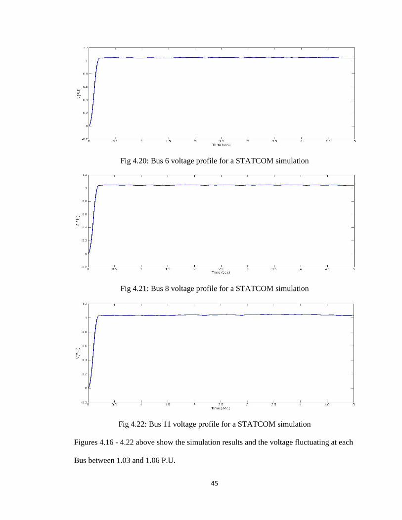
Fig 4.20: Bus 6 voltage profile for a STATCOM simulation
Fig 4.21: Bus 8 voltage profile for a STATCOM simulation
Fig 4.22: Bus 11 voltage profile for a STATCOM simulation
Figures 4.16 - 4.22 above show the simulation results and the voltage fluctuating at each
Bus between 1.03 and 1.06 P.U.
46
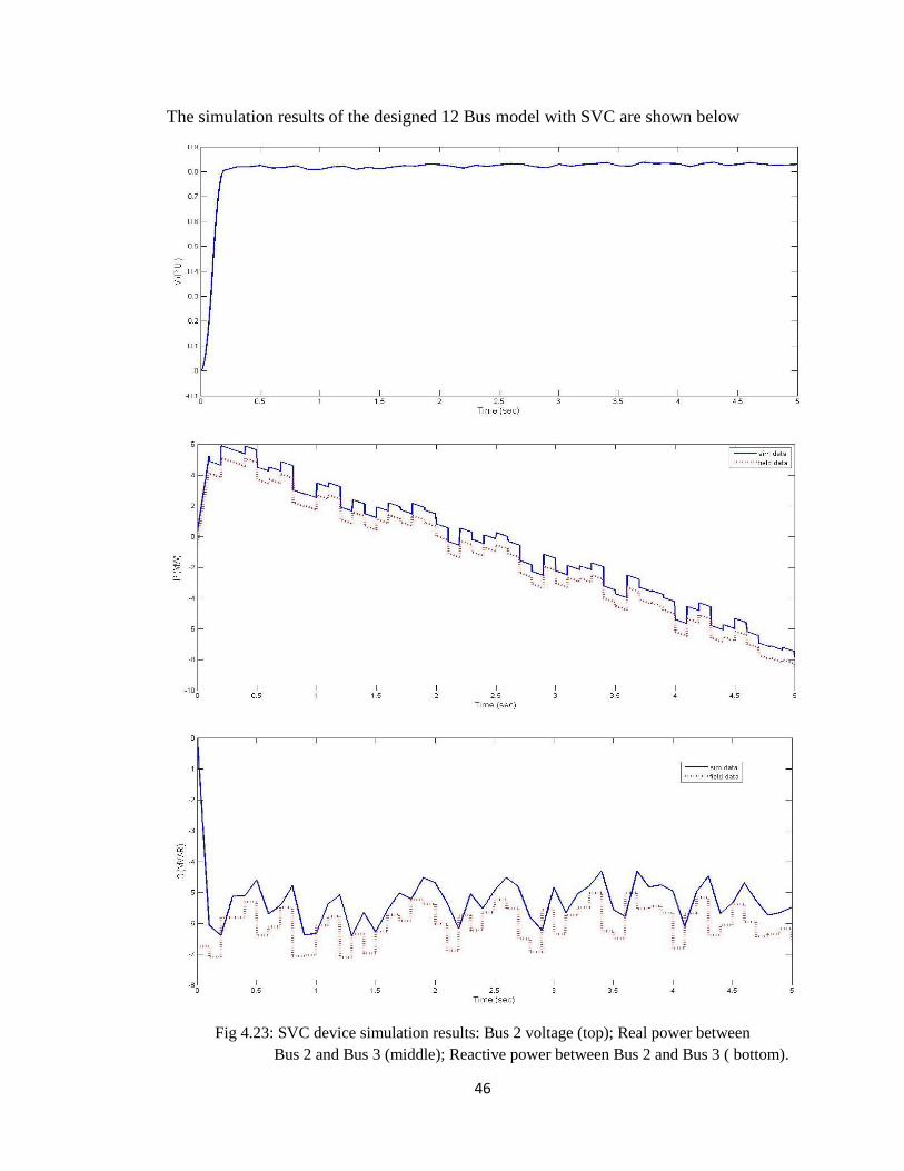
The simulation results of the designed 12 Bus model with SVC are shown below
Fig 4.23: SVC device simulation results: Bus 2 voltage (top); Real power between
Bus 2 and Bus 3 (middle); Reactive power between Bus 2 and Bus 3 ( bottom).
47
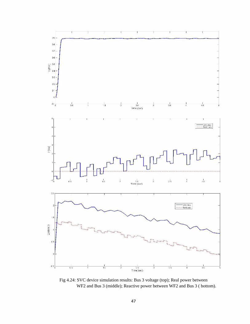
Fig 4.24: SVC device simulation results: Bus 3 voltage (top); Real power between
WF2 and Bus 3 (middle); Reactive power between WF2 and Bus 3 ( bottom).
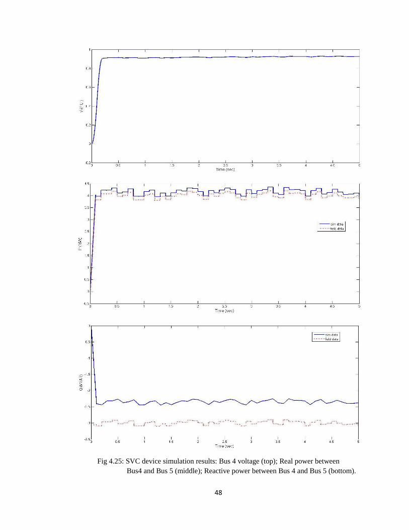
48
Fig 4.25: SVC device simulation results: Bus 4 voltage (top); Real power between
Bus4 and Bus 5 (middle); Reactive power between Bus 4 and Bus 5 (bottom).
49
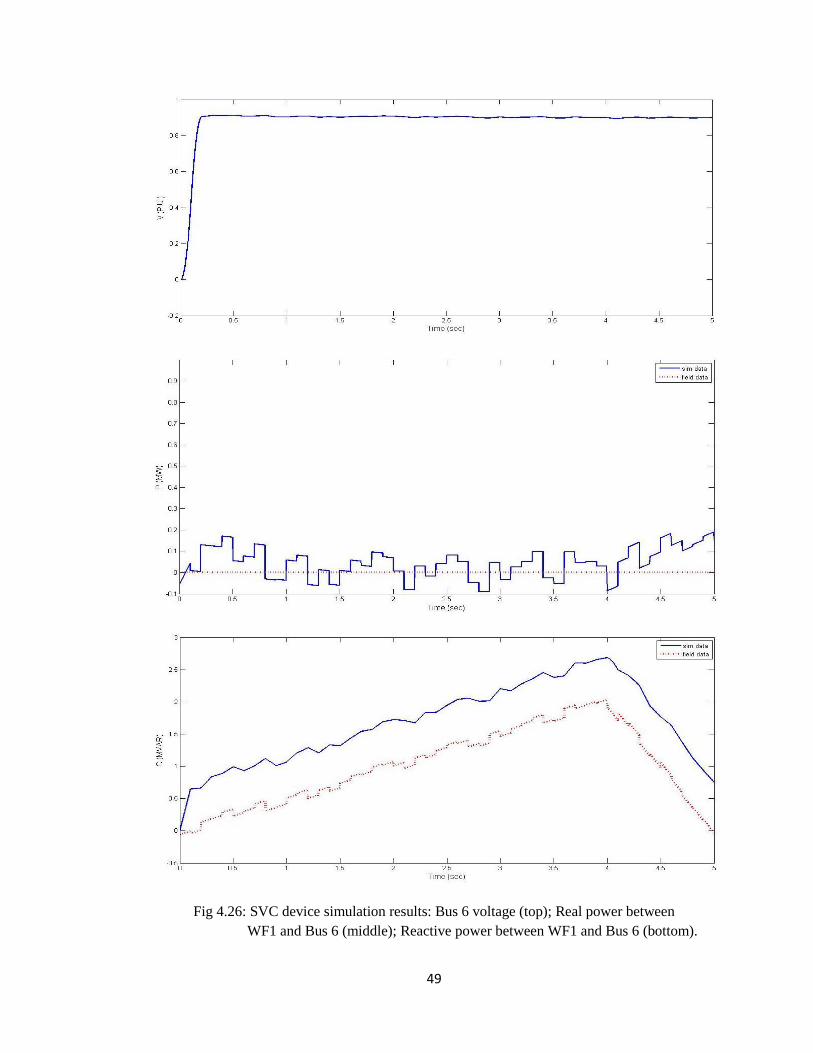
Fig 4.26: SVC device simulation results: Bus 6 voltage (top); Real power between
WF1 and Bus 6 (middle); Reactive power between WF1 and Bus 6 (bottom).

50
Figures 4.23 – 4.26 shows the voltage (V), real power (MW), reactive power (MVAR)
respectively between each Bus. The simulation results shown in figure 4.23 -4.26 show
some mismatch with the field data.
The mismatch at the beginning of each waveform is because of simulation
initialization constant. For real power in Fig 4.23 and 4.25 shows that there is a slight
mismatch in the results because the simulated loads are modeled as fixed loads. Because
of transformer reactance there is a constant offset of reactive power at Bus 6. The results
of 12 bus model with SVC doesn’t show much improvement when compared to the
results of model with STATCOM.
Voltage variations
Fig 4.27: Bus 2 voltage profile for a SVC simulation
51
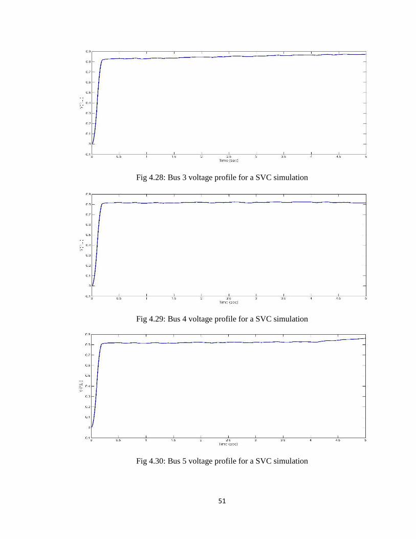
Fig 4.28: Bus 3 voltage profile for a SVC simulation
Fig 4.29: Bus 4 voltage profile for a SVC simulation
Fig 4.30: Bus 5 voltage profile for a SVC simulation
52
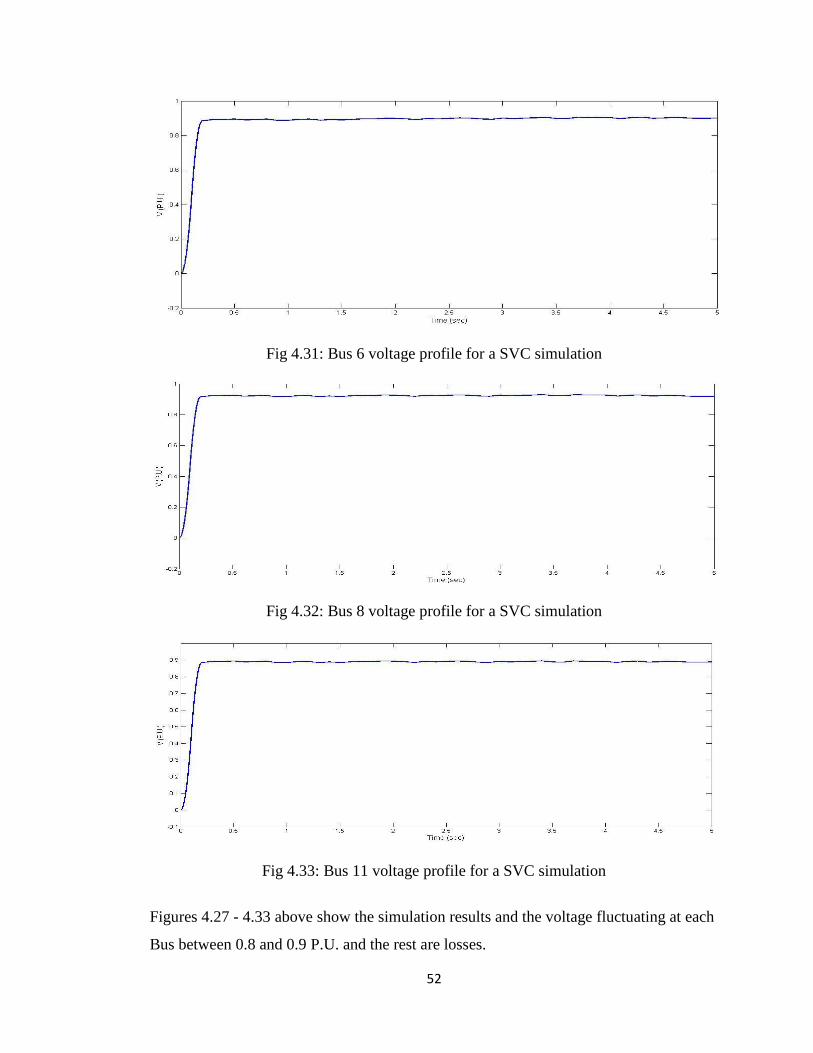
Fig 4.31: Bus 6 voltage profile for a SVC simulation
Fig 4.32: Bus 8 voltage profile for a SVC simulation
Fig 4.33: Bus 11 voltage profile for a SVC simulation
Figures 4.27 - 4.33 above show the simulation results and the voltage fluctuating at each
Bus between 0.8 and 0.9 P.U. and the rest are losses.

53
The simulation results of the designed 12 Bus model with SSSC are shown below
Fig 4.34: SSSC device simulation results: Bus 2 voltage (top); Real power between
Bus 2 and Bus 3 (middle); Reactive power between Bus 2 and Bus 3 ( bottom).

54
Fig 4.35: SSSC device simulation results: Bus 3 voltage (top); Real power between
WF2 and Bus 3 (middle); Reactive power between WF2 and Bus 3 ( bottom).
55
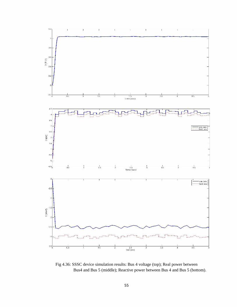
Fig 4.36: SSSC device simulation results: Bus 4 voltage (top); Real power between
Bus4 and Bus 5 (middle); Reactive power between Bus 4 and Bus 5 (bottom).

56
Fig 4.37: SSSC device simulation results: Bus 6 voltage (top); Real power between
WF1 and Bus 6 (middle); Reactive power between WF1 and Bus 6 (bottom).

57
Figures 4.34 – 4.37 shows the voltage (V), real power (MW), reactive power (MVAR)
respectively between each Bus. The simulation results shown in figure 4.34 -4.37 show
some mismatch with the field data.
The mismatch at the beginning of each waveform is because of simulation
initialization constants. Fig 4.34 and 4.36 shows that for real power there is slightly
mismatch in the results because the simulated loads are modeled as fixed loads. Because
of transformer reactance there is a constant offset of reactive power at Bus 6. The results
of 12 bus model with SSSC are as accurate as the results of 12 bus model with
STATCOM. Same as the results with STATCOM there is a constant increase in real
power in figure 4.36 between Bus 3 and wind farm 2 when compared with figure 4.2 i.e.
without any FACTS device. From figure 4.36 there is an increase in real power and
drops to 0 due to load impact and increases at 4 seconds.
Voltage Variations
Fig 4.38: Bus 2 voltage profile for a SSSC simulation

58
Fig 4.39: Bus 3 voltage profile for a SSSC simulation
Fig 4.40: Bus 4 voltage profile for a SSSC simulation
Fig 4.41: Bus 5 voltage profile for a SSSC simulation

59
Fig 4.42: Bus 6 voltage profile for a SSSC simulation
Fig 4.43: Bus 8 voltage profile for a SSSC simulation
Fig 4.44: Bus 11 voltage profile for a SSSC simulation
Figures 4.38-4.44 above show the simulation results and the voltage fluctuating at each
Bus between 1.0 –1.1 P.U.

60
The simulation results of the designed 12 Bus model with SSSC are shown below
Fig 4.45: UPFC device simulation results: Bus 2 voltage (top); Real power between
Bus 2 and Bus 3 (middle); Reactive power between Bus 2 and Bus 3 ( bottom).

61
Fig 4.46: UPFC device simulation results: Bus 3 voltage (top); Real power between
WF2 and Bus 3 (middle); Reactive power between WF2 and Bus 3 ( bottom).
62
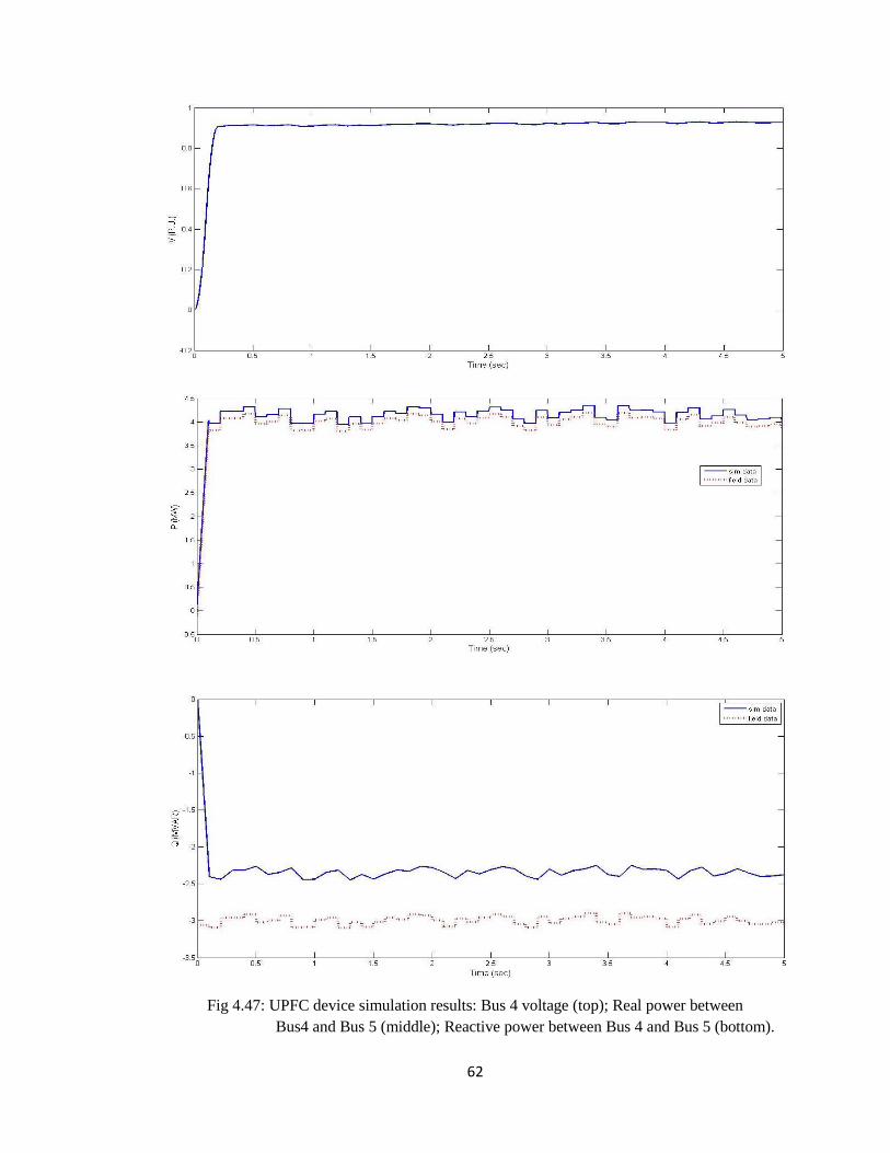
Fig 4.47: UPFC device simulation results: Bus 4 voltage (top); Real power between
Bus4 and Bus 5 (middle); Reactive power between Bus 4 and Bus 5 (bottom).
63
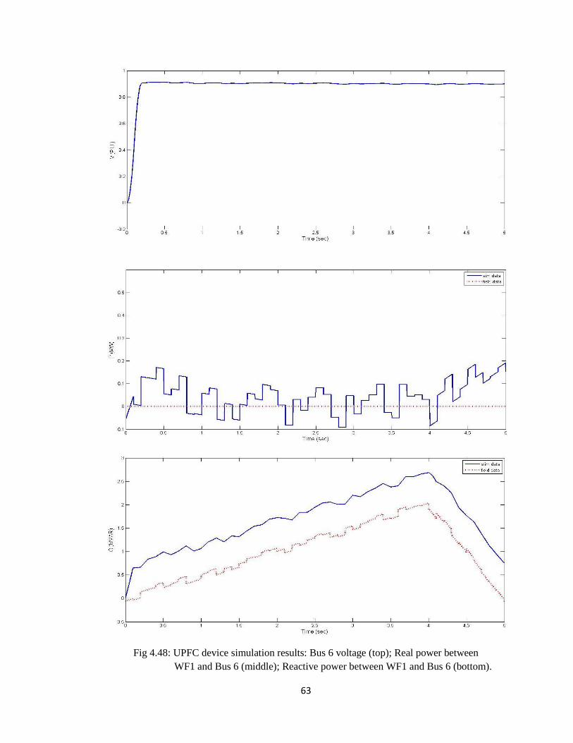
Fig 4.48: UPFC device simulation results: Bus 6 voltage (top); Real power between
WF1 and Bus 6 (middle); Reactive power between WF1 and Bus 6 (bottom).
64
Figures 4.45 – 4.48 shows the voltage (V), real power (MW), reactive power (MVAR)
respectively between each Bus. The simulation results shown in figure 4.45 -4.48 show
some mismatch with the field data.
The mismatch at the beginning of each waveform is because of simulation
initialization constant. Fig 4.45 and 4.47 shows that for real power there is slightly
mismatch in the results because the simulated loads are modeled as fixed loads. Because
of transformer reactance there is a constant offset of reactive power at Bus 6. The results
of the 12 bus model with UPFC are not accurate when compared to the model with
SSSC and STATCOM results.
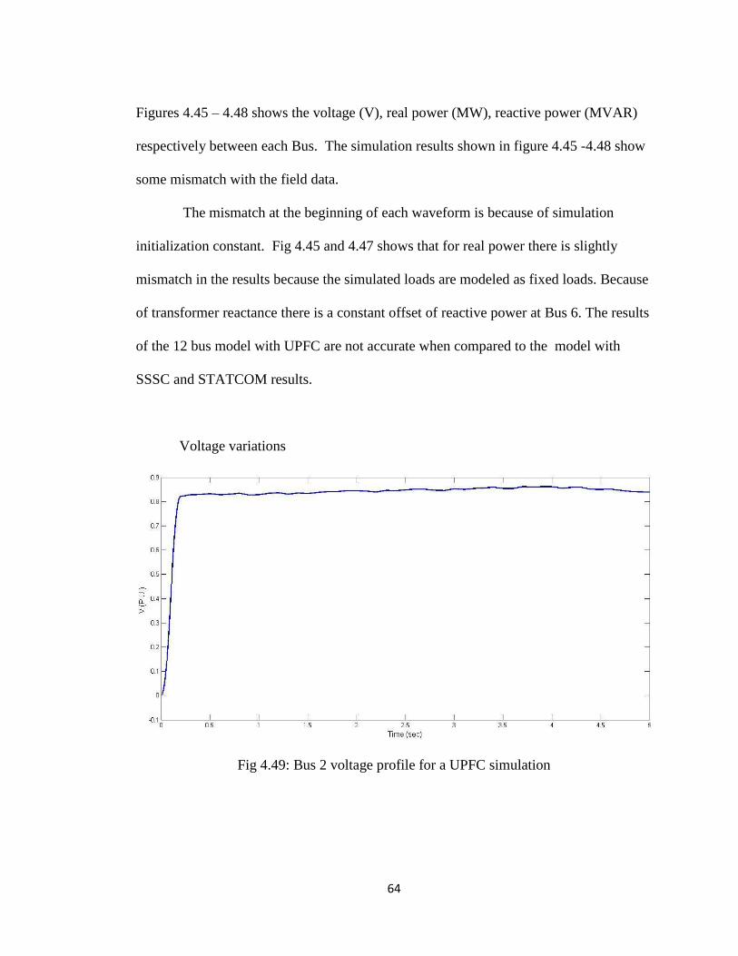
Voltage variations
Fig 4.49: Bus 2 voltage profile for a UPFC simulation
65
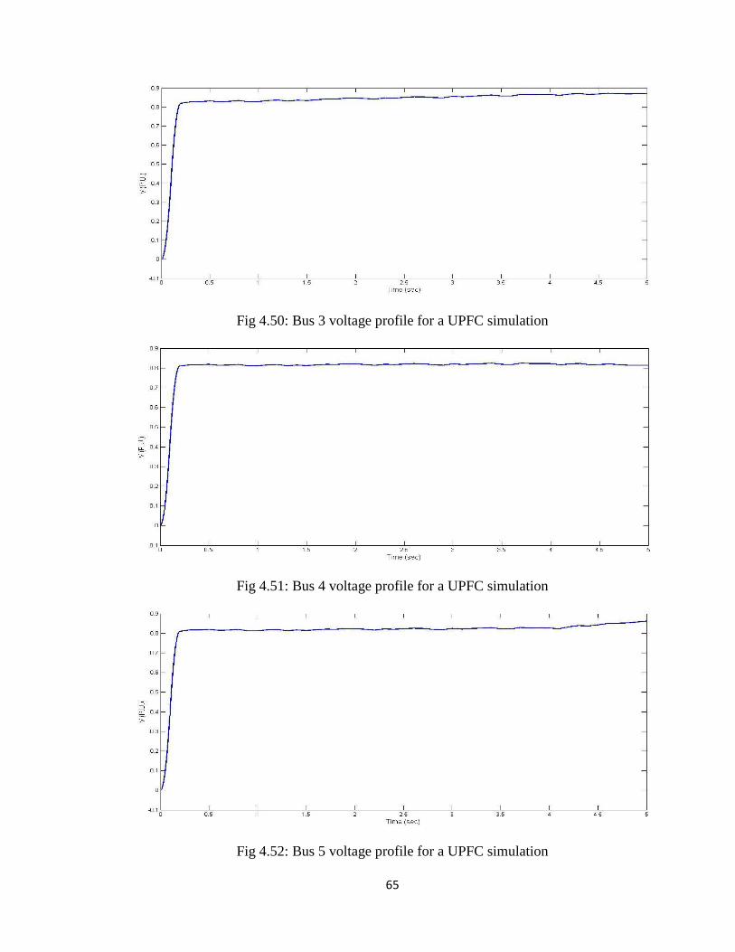
Fig 4.50: Bus 3 voltage profile for a UPFC simulation
Fig 4.51: Bus 4 voltage profile for a UPFC simulation
Fig 4.52: Bus 5 voltage profile for a UPFC simulation

66
Fig 4.53: Bus 6 voltage profile for a UPFC simulation
Fig 4.54: Bus 8 voltage profile for a UPFC simulation
Fig 4.55: Bus 11 voltage profile for a UPFC simulation
Figures 4.49-4.55 above show the simulation results and the voltage fluctuating at each
Bus between 0.83 –0.95 P.U.

67
Role of FACTS Devices
In order to discuss power quality improvement, the 12 Bus closed loop complex
system is designed and simulated by installing different FACTS devices at the weak
loop of the system. The various simulations are done by installing the FACTS devices
such as STATCOM, SVC, SSSC and UPFC in the closed loop system. By considering
the simulation results their voltage, real power and reactive power values at different
Buses are shown in Table 4.1 and Table 4.2 respectively
Table 4.1 Comparison of Simulation results with Field Data
Components
Bus2 to Bus 3
Bus 3 to WF2
Bus 4 to Bus 5
Wf1 to Bus 5
P
MW
Q MVA
V
P.U.
P
MW
Q
MVA
V
P.U.
P
MW
Q
MVA
V
P.U.
P
MW
Q
MVA
V
P.U.
Field Data 3.7 -6.8 1.05 -3.2 1.2 1.03 4.2 -3.2 1.01 0.0 1.1 1.02
Wind farm
Without FACTS 3.7 -6.1 0.83 0.5 1.3 0.91 3.9 -3.3 0.93 0.0
1.05
0.91
Wind Farm with
STATCOM
4.1
-6.4
1.05
3.3
1.6
1.03
4.5
-3.5
1.03
0.0
1.15
1.03
Wind farm
with SVC 3.5 -6.3
0.9
0.9
1.2
0.88
4.2
-3.6
0.93
0.0
1.07
0.95
Wind Farm with
UPFC 4.2 -6.5 0.93 1.1 1.5 0.92 4.2 -3.3 0.91 0.0 1.1 0.93
Wind Farm with
SSSC 4.2 -6.1 1.05 3.5 1.5 1.02 4,4 -3.5 1.05 0.0 1.09 1.05
Fuel cell with
STATCOM
3.9 -6.1 0.81 1.3 1.6 0.91 4.3 -3.3 0.88 0.0 1.1 0.91
PV with
STATCOM 4.2 -6.3 1.05 3.3 1.5 1.03 4.5 -3.6 1.04 0.0 1.1 1.045

68
Table 4.2 Voltage Profile at all Buses for Different Simulations Measured in (P.U.)
V( P.U.)
devices
V2(V)
V3(V)
V4(V)
V5(v)
V6(V)
V8(V)
V11(V)
without
FACTS
0.85
0.83
0.84
0.88
0.92
0.87
0.87
STATCOM 1.04 1.07 1.05 1.15 1.14 1.08 1.08
SVC
0.85
0.87
0.88
0.9
0.92
0.9
0.9
SSSC
1.04
1.03
1.05
1.15
1.15
1.08
1.08
UPFC
0.87
0.88
0.91
0.93
0.93
0.89
0.89
PV
1.02
1.05
1.04
1.09
1.11
1.08
1.08
Fuel cell
0.85
0.84
0.85
0.89
0.92
0.88
0.88
From the above tables it is clear that with installation of FACTS device there is
an improvement in power quality. A change in voltage variation is observed with the
installation of FACTS. From the above tables it is clear that the STATCOM and SSSC
show better improvement in power quality when compared to SVC and UPFC. For
achieving better results with SVC, a higher rated SVC has to be chosen. The reason for
the degraded results of UPFC is that the model is designed with normal converters rather
than multi level converters. From the Table 4.2 it is observed that there is an
improvement in power quality with the photovoltaic model when compared to the fuel
cell model because voltage variations of photovoltaic model are similar to the wind farm
model with STATCOM where as the fuel cell model doesn’t show much improvement.

69
The total harmonic distortion at different Buses are simulated and their values are shown
in Table 4.3.
Table 4.3 Total Harmonic Distortion at Different Buses
THD
Devices
B1
B3
B5
B6
B8
B12
Without FACTS
24.95
24.9
24.94
25.04
24.94
24.95
STATCOM 0.21 0.39 0.86 0.64 0.86 0.21
SVC 10.36 10.33 10.31 10.33 10.31 10.36
SSSC 10.38 10.43 10.43 11.25 10.58 10.38
UPFC 10.36 10.36 10.36 10.35 10.36 10.36
From the above table it is clear that the wind farm model with STATCOM
reduces harmonic content to some extent when compared to other FACTS devices. The
other FACTS devices also help in reducing the harmonic content when compared to the
model without any FACTS device, but not as good as the model with STATCOM.
Voltage Stability
Voltage stability is the ability of a power system to maintain steady voltages at
all Buses in the system after being subjected to a disturbance. Voltage instability occurs
when there are sudden changes in voltage at different Buses due to disturbance. A
possible outcome of voltage instability is the tripping of transmission lines and other
elements by their protective systems. Loss of synchronism of some generators may

70
result from reaching the generator field current limit. The voltage stability is of two
types: large disturbance voltage stability and small disturbance voltage stability.
Large-disturbance voltage stability refers to the ability of the system to maintain
steady voltages under large disturbances such as system faults, loss of generation, or
circuit contingencies. This can be determined by the system and load characteristics. It
also requires an examination of the nonlinear response of the power system over a
period of time, sufficient to capture the performance and interactions of devices such as
motors, under-load transformer tap changers and generator field-current limiters.
Small-disturbance voltage stability refers to the system's ability to maintain
steady voltages when subjected to small disturbance such as incremental changes in
system load. This form of stability is influenced by the characteristics of loads,
continuous controls, and discrete controls. This concept is useful in determining how the
system voltages will respond to small system changes.
P-V Curves
The voltage stability analysis process involves the transfer of power from one
region of a system to another and monitoring the effects to the system voltages. A
typical PV curve is shown in Fig 4.56. From the Figure it is observed that at the bottom
of the PV curve, the voltage drops rapidly when there is an increase in the load demand.
If the load flow solutions converge beyond this point, then the system has become
unstable. This point is known as the critical point. This curve can be used to determine
the system’s critical operating voltage and collapse margin. The operating points above
the critical point signify a stable system. If the operating points are below the critical
point, the system is said to be in an unstable condition.
71
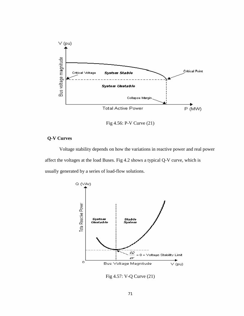
Fig 4.56: P-V Curve (21)
Q-V Curves
Voltage stability depends on how the variations in reactive power and real power
affect the voltages at the load Buses. Fig 4.2 shows a typical Q-V curve, which is
usually generated by a series of load-flow solutions.
Fig 4.57: V-Q Curve (21)

72
From the Figure 4.57 it is observed that voltage stability limit is at the point
where the derivative dQ/dV is equal to zero. An increase in reactive power will result in
an increase in voltage during normal operating conditions. Hence, if the operating point
is on the right side of the voltage stability limit, the system is said to be stable and if
operating point is on left side of the graph the voltage stability limit, the system is said
to be unstable .
Stability Curves
The stability curves with and without FACTS device are shown in Figures 4.58–4.67
Stability curves of 12 Bus model without any FACTS device shown below
Fig 4.58: PV curve or nose curve for wind farm1 without FACTS
73
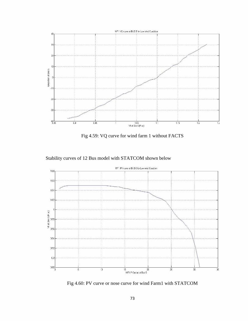
Fig 4.59: VQ curve for wind farm 1 without FACTS
Stability curves of 12 Bus model with STATCOM shown below
Fig 4.60: PV curve or nose curve for wind Farm1 with STATCOM

74
Fig 4.61: VQ curve for wind farm 1 with STATCOM
Stability curves of 12 Bus model with SVC shown below
Fig 4.62: PV curve or nose curve for wind farm1 with SVC
75
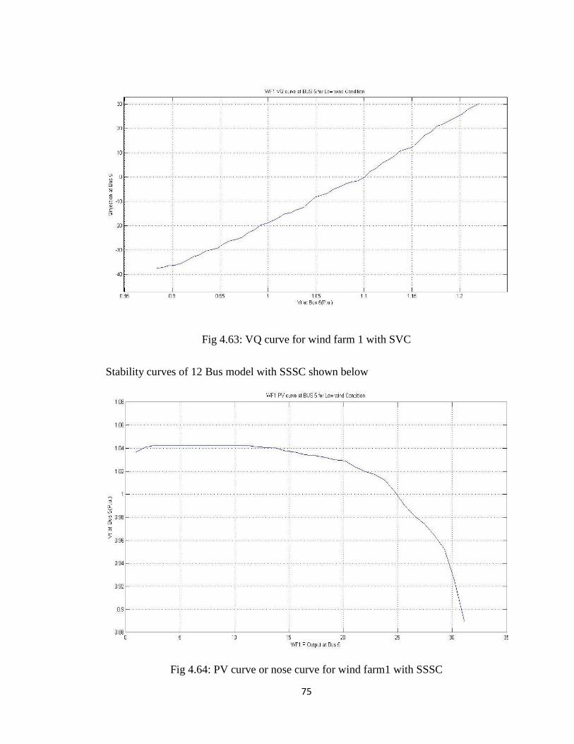
Fig 4.63: VQ curve for wind farm 1 with SVC
Stability curves of 12 Bus model with SSSC shown below
Fig 4.64: PV curve or nose curve for wind farm1 with SSSC

76
Fig 4.65: VQ curve for wind farm 1 with SSSC
Stability curves of 12 Bus model with UPFC shown below
Fig 4.66: PV curve or nose curve for wind farm1 with UPFC

77
Fig 4.67: VQ curve for wind farm 1 with UPFC
The PV and VQ curve at WF1 are generated and observed from Fig 4.58-4.67. The PV
curve is obtained by regulating the WF1 source angle to increase the real power
injection at bus 6 while keeping the rest of the system constant.. The PV curve is
obtained by increasing the wind farm one for more voltage stability. It is clear that the
WF1 injects unity power factor power (0.88P.U.) at about 31.5 MW of power injected at
this Bus for voltage stability. The MSCs of WF1 act as a power factor compensator and
can further improve the PV curve and also source angle to inject the real power, while
the rest of the system is maintained constant. Therefore, the voltage stability is not a
serious issue for this closed loop system. The FACTS device using its fast response
focuses on solving the dynamic voltage fluctuation rather than concentrating on a steady
state voltage profile. The VQ curve which is obtained by injecting VAR on Bus 5 helps
to represent the size of the FACTS device. The VQ curve also indicates that there is no
voltage stability issue at the operating point .

78
CHAPTER FIVE
Conclusions and Future Work
The increasing penetration of renewable energy sources, growing demands,
limited sources, and deregulated electricity markets have caused new challenges to the
operation, control and stability of modern electric power systems. This study
investigates the application of FACTS devices to enhance the dynamic and transient
performance of power systems with a large share of distributed energy resources, which
includes large renewable sources such as wind farms. FACTS devices such as
STATCOM, SVC, SSSC, UPFC are placed at suitable locations in a 12-Bus multi-
machine power system model with large renewable energy sources. Simulations show
that there is a significant improvement in power quality due to the FACTS devices. The
developed model is stable with and without FACTS devices. When comparing FACTS
devices for better power quality and voltage stability, it is clear that STATCOM and
SSSC are superior to other FACTS devices. However, in this study the UPFC Simulink
model was further modified in order to be able to get better results. Moreover the rating
of SVC used in this study is the same as that of STATCOM. The rating of SVC has to be
increased more than the rating of STATCOM for getting better power quality
improvement.
The performance of photovoltaic cell and fuel cell stacks with a STATCOM
device was studied. From the simulation results it is observed that there is an

79
improvement in power quality with photovoltaic cells but there is no significant
improvement using fuel cell stack when compared to that of wind farms and
photovoltaic arrays.
The harmonic analysis at different Buses has to be studied with all renewable
energy sources and different FACTS devices. The power quality and voltage stability of
photovoltaic cells and fuel cell stacks with various FACTS devices are to be studied and
compared. The power quality and voltage stability of large power systems with biomass
Distributed energy resources (DERS) with different FACTS device has to be studied.
Voltage stability of power systems with a large share of DERS need to be studied further
along with optimization of FACTS devices location.
80
REFERENCES
[1] D. Seifried and W. Witzel, Renewable Energy – The FACTS, Earthscan, Third edition, 2010.
[2] Stanley R. Bull, “Renewable Energy Today and Tomorrow” Proceedings of the
IEEE, vol. 89, no. 8, August 2001.
[3] Thomas Ackerman, Wind power in Power Systems, Wiley, 2005.
[4] James larminie, “Fuel cell Systems Explained”, Second Edition, Wiley, 2003.
[5] Yun Tiam Tan; Kirschen, D.S. , “Impact on the Power System of a Large Penetration
of Photovoltaic Generation,” Power Engineering Society General Meeting, 2007
IEEE , vol., no., pp.1-8, 24-28 June 2007.
[6] N. G. Hingorani and L. Gyugyi, Understanding FACTS: Concepts and Technology
of Flexible AC Transmission Systems, IEEE Press, 2000.
[7] Yong Hua Song and Allan T Johns, Flexible AC Transmission Systems (FACTS),
IEEE power and energy series, first edition,1999.
[8]Musunuri, S.; Dehnavi, G., “Comparison of STATCOM, SVC, TCSC, and SSSC
performance in steady state voltage stability improvement,” North American Power
Symposium (NAPS), 2010, vol., no., pp.1-7, 26-28 Sept. 2010.
[9] Ciausiu, F.E.; Eremia, M.; , "Improvement of power systems security margins by
using FACTS devices," PowerTech, 2011 IEEE Trondheim , vol., no., pp.1-7, 19-23
June 2011.
81
[10] A. Kehrli, M. Ross, “Understanding grid integration issues at wind farms and
solutions using voltage source converter FACTS technology,” IEEE PES General
Meeting, vol. 3, pp. 1822-1827, July 2003.
[11] Salim. Haddad, A. Haddouche, and H.Aouyeda, “ The use of FACTS Devices in
Disturbed Power Systems- Modeling, Interface, and Case Study” International
Journal of Computer and Electrical Engineering, Vol. 1, No. 1, pp. 56-60, April
2009.
[12] Chong Han; Huang, A.Q.; Litzenberger, W.; Anderson, L.; Edris, A.-A.; Baran, M.;
Bhattacharya, S.; Johnson, "STATCOM Impact Study on the Integration of a Large
Wind Farm into a Weak Loop Power System," PSCE '06. 2006 IEEE PES, vol.,
no., pp.1266-1272, Oct. 29 2006-Nov. 1 2006.
[13] Wei Qiao; Harley, R.G.; Venayagamoorthy, G.K. , “Effects of FACTS Devices on
a Power System Which Includes a Large Wind Farm,” Power Systems Conference
and Exposition, 2006. PSCE '06. 2006 IEEE PES , vol., no., pp.2070-2076, Oct. 29
2006-Nov. 1 2006.
[14] Bowen Wu; Yue Yuan; Qiang Li; Zhenjie Li; Weisheng Wang; , "Estimation of the
Power Quality problem Caused by Large Wind Farm: A real case study," IPEC,
2010 Conference Proceedings , vol., no., pp.773-776, 27-29 Oct. 2010.
[15] Hansen, A.D.; Sorensen, P.; Janosi, L.; Bech, J.; , "Wind farm modelling for power
quality," Industrial Electronics Society, 2001. IECON '01. The 27th Annual
Conference of the IEEE , vol.3, no.9, pp.1959-1964 vol.3, 2001.
[16] Yuvaraj, V.; Deepa, S.N.; Rozario, A.P.R.; Kumar, M.; , "Improving Grid Power
Quality with FACTS Device on Integration of Wind Energy System," Modelling
Symposium (AMS), 2011 Fifth Asia , vol.3, no.4, pp.157-162, 24-26 May 2011.

82
[17] Kuiava, R.; Ramos, R.A.; Bretas, N.G.; , "Control design of a STATCOM with
Energy Storage System for stability and power quality improvements," Industrial
Technology, 2009. ICIT 2009. IEEE International Conference on , vol., no., pp.1-6,
10-13 Feb. 2009.
[18] Wei Qiao; Harley, R.G.; , "Power Quality and Dynamic Performance Improvement
of Wind Farms Using a STATCOM," Power Electronics Specialists Conference,
2007. PESC 2007. IEEE , vol., no., pp.1832-1838, 17-21 June 2007.
[19] L. T. Ha, T. K. Saha, “Investigation of Power Loss and Voltage Stability Limits for
large Wind Farm Connections to a Subtransmission Network,” IEEE PES General
Meeting, vol.2, pp. 2251-2256, June 2004.
[20] F. Zhou, G. Joos, C. Abbey, “Voltage Stability in Weak Connection Wind Farms,”
IEEE PES General Meeting, pp. 610-615, June 2005.
[21] Salehi, V.; Afsharnia, S.; Kahrobaee, S.; , "Improvement of Voltage Stability in
Wind Farm Connection to distribution Network Using FACTS Devices," IEEE
Industrial Electronics, IECON 2006 - 32nd Annual Conference on , vol., no.,
pp.4242-4247, 6-10 Nov. 2006.
[22] Gupta, S.; Tripathi, R.K.; Shukla, R.D.; , "Voltage stability improvement in power
systems using facts controllers: State-of-the-art review," Power, Control and
Embedded Systems (ICPCES), 2010 International Conference on , vol., no., pp.1-8,
Nov. 29-2010Dec. 1 2010.
[23] Haque, M.H.; , "Stability improvement by FACTS devices: a comparison between
STATCOM and SSSC," Power Engineering Society General Meeting, 2005.
IEEE , vol., no., pp. 1708-1713 Vol. 2, 12-16 June 2005.
[24] Galu, Y.; Munda, J.L.; Jimoh, A.A.; , "Stability improvement of Centurion electric
power network using FACTS controllers," Power and Energy Conference, 2008.
PECon 2008. IEEE 2nd International , vol., no., pp.1350-1353, 1-3 Dec. 2008.

83