poverty trends in nepal (1995-96 and 2003-04)cbs.gov.np/image/data/publication/others/poverty...
TRANSCRIPT
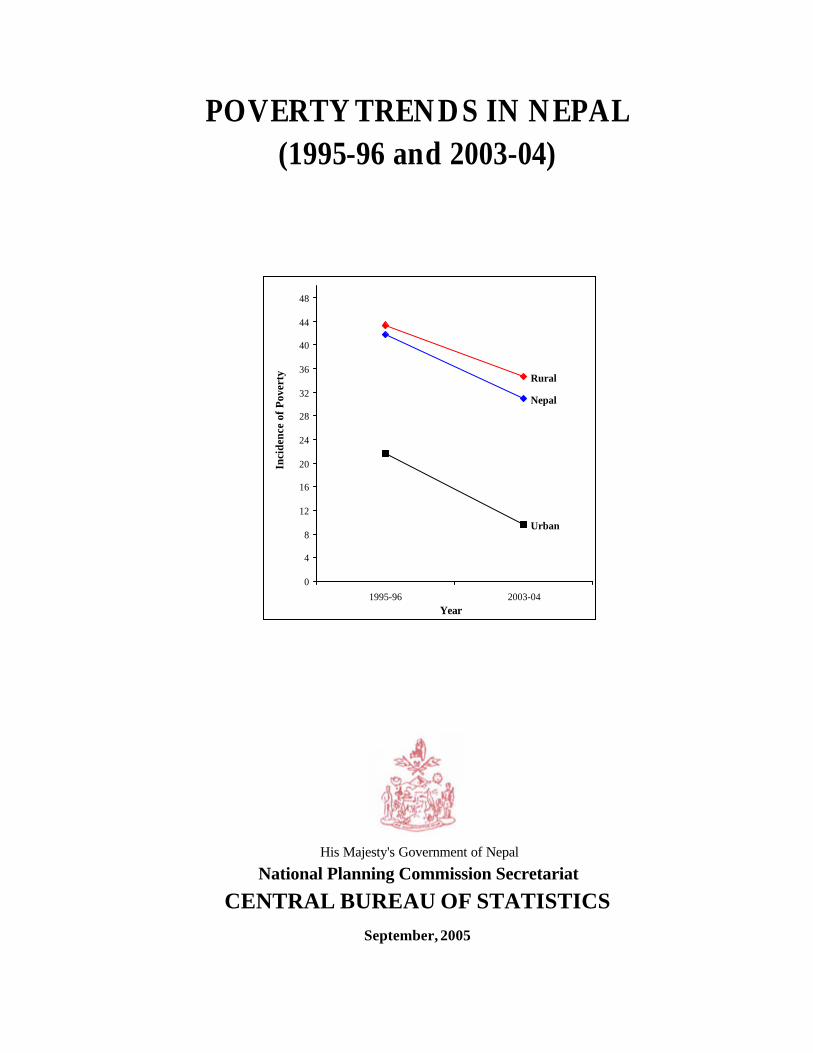
POVERTY TRENDS IN NEPAL (1995-96 and 2003-04)
His Majesty's Government of Nepal
National Planning Commission Secretariat
CENTRAL BUREAU OF STATISTICS
September, 2005
Nepal
Rural
Urban
0
4
8
12
16
20
24
28
32
36
40
44
48
1995-96 2003-04Year
Inci
denc
e of
Pov
erty
POVERTY TRENDS IN NEPAL (1995-96 and 2003-04)
His Majesty's Government of Nepal
National Planning Commission Secretariat
CENTRAL BUREAU OF STATISTICS
September, 2005
Published by: Central Bureau of Statistics Thapathali, Kathmandu, Nepal Phone: 4229406, 4241803, 4245946-48 Fax: 977-1-4227720 E-mail: [email protected] First Edition: September, 2005 1,000 copies Printed by: ……….., Kathmandu Nepal Phone: …………….

i
ii
Preface Central Bureau of Statistics carried out Nepal Living Standards Survey 2003-04, a nation-wide multi-purpose household expenditure and income survey, as a follow up of the first survey conducted in 1995-96. The statistical reports containing the major findings of the survey were published in two volumes by the Bureau in December 2004. This report presents NLSS-based poverty results estimated using the cost-of-basic needs (CBN) methodology and also the poverty trends in Nepal between 1995-96 and 2003-04. In order to maintain the comparability of the 2003-04 results with the 1995-96 estimates of poverty in the country, poverty lines were derived to adjust for regional differences in cost-of-living and inter-temporal inflation. There are two chapters in the report. Included in the first chapter are poverty incidence, growth and inequality, poverty profile and multivariate analysis of poverty, sensitivity and robustness of poverty estimates and other evidences in support of poverty measurements. Second chapter describes the methodology used to derive regional and inter-temporal poverty lines, and presents the various region and time-specific poverty lines for food, non-food and overall consumption aggregates. Results indicate that poverty incidence in the country declined appreciably, from 42 percent in 1995-96 to 31 percent in 2003-04 and various sensitivity analy ses confirm the robustness of these trends. On the other hand, as a result of unequal growth in per capita consumption across different income groups and geographic regions, inequality increased substantially. This work is the product of collaboration between the World Bank, DFID and Central Bureau of Statistics (CBS). I would like to sincerely thank the World Bank team led by Elena Glinskaya (Sr. Economist, SASPR). The World Bank team included Michael Lokshin (Sr. Economist, DEC), Dilip Parajuli (Consultant, SASPR, DFID-Nepal) and Mikhail Bontch Osmolovski (Consultant, SASPR). I wholeheartedly appreciate the CBS team that consisted of Uttam Narayan Malla (Deputy Director General), Krishna Prasad Shrestha (the then Deputy Director and head of household survey section), Rabi Prasad Kayastha, Present Deputy Director of the Survey Section and Statistical Officers Ram Hari Gaihre, Ishwori Prasad Bhandari, Anil Sharma, Guna Nidhi Sharma, Binod Manandhar, Kapil Prasad Timalsena and Computer Assistant Mohan Khajum Chongbang. September, 2005 Tunga S. Bastola
Director General Central Bureau of Statistics
iii
CONTENT
Page
Chapter I : Poverty Trends in Nepal between 1995-96 and 2003-04 ...... 1
1.1 Introduction .........................................................................................................1
1.2 Incidence of Poverty in Nepal in 1995-96 and 2003-04 ...........................................2
1.3 Growth and Inequality: Changes between 1995-96 and 2003-04 ..............................5
1.3.1 Trends in Real Expenditure................................ ................................ ..........5
1.3.2 The Relationship between Growth in Per-capita Expenditure and Poverty ......8
1.3.3 Growth Incidence Curves ...........................................................................9
1.3.4 Inequality ................................ ................................ ................................ 11
1.3.5 Poverty Decomposition: Growth and Inequality........................................... 12
1.3.6 Poverty Decomposition: Regional............................................................... 13
1.4 Poverty Profile and Multivariate Analysis of Poverty................................ ............ 15
1.4.1 Poverty Profile ................................ ................................ ........................ 15
1.4.2 Multivariate Poverty Profile and Simulations .............................................. 22
1.5 Sensitivity and Robustness of Poverty Estimates ................................................... 24
1.5.1 Poverty Incidence Curves .......................................................................... 25
1.5.2 “Missing PSUs” ....................................................................................... 27
1.5.3 Alternative Approaches to Defining Poverty Lines ..................................... 29
1.6 Other Evidence of Changes in Living Standards .................................................. 32
1.6.1 Subjective Poverty Line ................................ ................................ ............ 33
1.6.2 Trends in Quantities of Foods Consumed ................................ .................... 35
1.6.3 Evidence from a Panel Sample ................................................................. 37
1.6.4 Trends in Agricultural Wages ..................................................................... 38
1.6.5 Trends in Income Poverty .......................................................................... 39
1.7 Tentative Explanations for the Observed Increase in Per-capita Income and Expenditure and Decline in Poverty ..................................................................... 40
iv
Page
Chapter II : The Methodology used to Derive Poverty Lines (1995-96 and 2003-04).......................................................47
2.1 An Overview of the Methodology................................ ................................ ........ 47
2.2 Deriving the Poverty Lines: A more Detailed Exposition...................................... 49
2.2.1 Deriving the Food Price Indices ................................ ................................ 49
2.2.2 Deriving the Non-Food Price Indices .......................................................... 52
2.2.3 Aggregating the Food and Non-food Poverty Line Components.................. 54
2.3 Region and Time-specific Poverty Lines and Overall Price Index ......................... 56
v
LIST OF TABLES Chapter I Page
Table 1.2.1 : Nepal 1995-96 and 2003-04, Poverty Measurement.......................................2
Table 1.2.2 : Nepal 1995-96 and 2003-04, Poverty Measurement by Geographic Regions.......................................................................................................4
Table 1.3.1 : Nepal 1995-96 and 2003-04, Distribution of Real (1995-96 average Nepal prices) Per-capita Expenditure .....................................................................6
Table 1.3.2 : Nepal 1995-96 and 2003-04, NLSS PCE versus National Accounts Per Capita GDP and Per Capita Private Consumption ................................ ..........7
Table 1.3.3 : Nepal 1995-96 and 2003-04, Ratio of PCE at Selected Percentiles and Gini Coefficients ....................................................................................... 11
Table 1.3.4 : Nepal 1995-96 and 2003-04, PCE at Selected Percentiles in Urban Areas over the Same PCE Percentile in Rural Areas .............................................. 12
Table 1.3.5 : Nepal, Growth and Redistribution Decomposition of Poverty Changes between 1995-96 and 2003-04................................ ................................ .... 13
Table 1.3.6 : Nepal: 1995-96 and 2003-04, Regional Poverty Decomposition.................... 14
Table 1.4.1 : Nepal 1995-96 and 2003-04, Poverty Measurement by Employment Sector of the Household Head ................................ ................................ .... 16
Table 1.4.2 : Nepal 1995-96 and 2003-04, Poverty Measurement by Education Level of the Household Head................................................................................... 17
Table 1.4.3 : Nepal 1995-96 and 2003-04 Poverty Measurement by HH Head’s Age and Sex ........................................................................................................... 18
Table 1.4.4 : Nepal 1995-96 and 2003-04 Poverty Measurement by Demographic Composition.............................................................................................. 19
Table 1.4.5 : Nepal 1995-96 and 2003-04, Poverty Measurement by Caste and Ethnicity of the Household Head............................................................................... 21
Table 1.4.6 : Nepal 1995-96 and 2003-04 Poverty Measurement, by Land Ownership (rural areas only) ....................................................................................... 22
Table 1.4.7 : Nepal 2003-04, Changes in the Probability of being in Poverty (percent)....... 23
Table 1.5.1 : Nepal 1995-96 and 2003-04, Sensitivity of Headcount Poverty Rate with Respect to the Choice of Poverty Line......................................................... 27
vi
Table 1.5.2 : Nepal 1995-96 and 2003-04, Sensitivity of Headcount Poverty Rate with Respect to Poverty Rates in Missing PSUs .................................................. 29
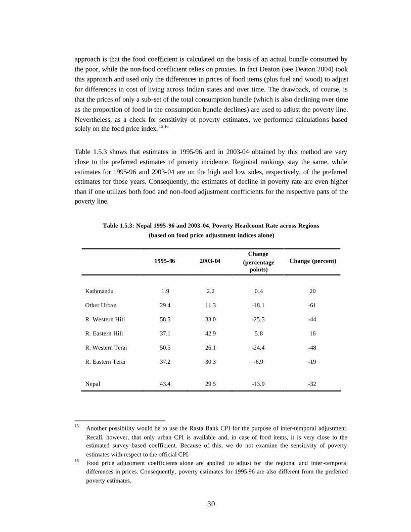
Table 1.5.3 : Nepal 1995-96 and 2003-04, Poverty Headcount Rate across Regions (based on food price adjustment indices alone) ................................ ............ 30
Table 1.5.4 : Nepal 1995-96 and 2003-04, “Food Poverty” Headcount Rate across Regions..................................................................................................... 31
Table 1.5.5 : Nepal 1995-96 and 2003-04, A-Dollar-Day Poverty Rates ............................ 32
Table 1.6.1 : Nepal 1995-96 and 2003-04, Self-reported Assessment of Consumption Adequacy.................................................................................................. 33
Table 1.6.2 : Nepal 1995-96 and 2003-04, Subjective Poverty.......................................... 34
Table 1.6.3 : Nepal 1995-96 and 2003-04, Consumption of Selected Foods (grams, per person, per month) ................................ ................................ .................... 35
Table 1.6.4 : Nepal 1994-95 and 2003-04, Transition Matrix in and out of Poverty (Panel sample) ........................................................................................... 37
Table 1.6.5 : Nepal 1995-96 and 2003-04 Agricultural Wages by Geographic Region (rural areas) ............................................................................................... 39
Table 1.6.6 : Nepal 1995-96 and 2003-04, Income-based Poverty Estimates ..................... 40
Table 1.7.1 : Nepal 1995-96 and 2003-04, Remittances Received by Households .............. 41
Table 1.7.2 : Nepal 1995-96 and 2003-04, Regional Patterns of Remittances..................... 42
Table 1.7.3 : Nepal 1995-96 and 2003-04, Sources of Households’ Income....................... 43
Table 1.7.4 : Nepal 1995-96 and 2003-04 Income from Non-agricultural Sources.............. 44
Table 1.7.5 : Nepal 1995-96 and 2003-04, Inverse Dependency Ratio ............................... 46
Chapter II
Table 2.2.1 : Nepal 1995-96 and 2003-04, Regional Food Price Indices ........................... 51
Table 2.2.2 : Nepal 1995-96 and 2003-04, Regional Non-Food Price Indices ................... 53
Table 2.3.1 : Nepal 1995-96 and 2003-04,Poverty Lines in Current Prices per Person per ........................................................................................................... 56
Table 2.3.2 : Nepal 1995-96 and 2003-04: Overall Price Indices (Relative to 1995-96 rural Eastern Terai and relative to 1995-96 all-Nepal average) ...................... 57
vii
LIST OF FIGURES AND BOXES Chapter I Page
Figure 1.2.1 : Growth Incidence Curves, All Nepal and Urban and Rural areas ................... 10
Figure 1.5.1 : Cumulative Distributions of Annual Real PCE: National, Urban, and Rural... 26
Figure 1.6.1 : Nepal 1995-96 and 2003-04, Consumption of Selected Foods by Deciles of PCE...................................................................................................... 36
Box 1.1 : Definition of Geographic Regions in Nepal...................................................3
Box 1.4.1 : Proportion of Households Receiving Remittances by the Household Heads’ Age and Sex................................................................................... 17
Box 1.4.2 : Comparison of Caste and Ethnicity between NLSS -I and II.......................... 20
Chapter I
Box 2.1 : Deriving the 1995-96 Rural Eastern Terai Poverty Line: A Brief Synopsis .... 48
Box 2.2 : Adjusting for Changes over Time in Nepal’s Demographic Composition ...... 55
viii
ANNEXES
ANNEX I Page
Figure A1.1 : Growth Incidence Curves for 6 NLSS regions of Nepal................................ 58
Figure A1.2 : Cumulative Distributions of Annual Real PCE for 6 NLSS Regions of Nepal................................ ................................ ................................ ........ 59
Figure A1.3 : Rural Eastern Terai, Poverty Incidence, Poverty Deficit and Poverty Severity Curves ......................................................................................... 60
Table A1.1 : Nepal 1995-96 and 2003-04, Consumption of Selected Foods (grams, per person, per month)..................................................................................... 61
ANNEX II
Table A2.1 : Nepal, Food Basket Composition of Poverty Line, NLSS1 and NLSS2......... 62
Table A2.2 : Nepal, Food Quantity Conversion Factors from “Manna” to Grams .............. 63
Table A2.3 : Nepal, Food Quantity Conversion from Units to Grams................................ 64
Table A2.4 : Nepal 1995-96 and 2003-04 LSS-I and NLSS II-Based Food Unit Prices and Quantities Consumed........................................................................... 65
Table A2.5 : Nepal, Changes between 1995-96 and 2003-04 in NLSS-I and NLSS-II-Based Food Unit Prices and Quantities Consumed ....................................... 66

1
CHAPTER I
Poverty Trends in Nepal between 1995-96 and 2003-04
1.1 Introduction
This chapter presents results on the extent and profile of poverty in Nepal in 2003-04 as well as the changes that have occurred since 1995-96, when the last poverty profile was developed. The poverty line for Nepal has been derived on the basis of the 1995-96 Nepal Living Standards Survey (NLSS-I) using the cost-of-basic-needs (CBN) method. Changes in the cost of living have been taken into account using region-specific price indices developed on the basis of NLSS-I 1995-96 and NLSS-II 2003-04.
The World Bank Poverty Assessment report, “Nepal: Poverty at the Turn of the Twenty-First Century,” estimated the incidence of poverty in Nepal at 42 percent in 1995-96.1 During the 8 years between 1995-96 and 2003-04 the Nepalese economy performed well, with real gross domestic product (GDP) growing at almost 5 percent per year (2.5 percent per capita per year). Annual agricultural growth accelerated to 3.7 percent in the second half of the 1990s (or about 1.5 percent per year in per-capita terms). Growth also accelerated in manufacturing (led by exports), in services, and especially in tourism. Remittances from abroad soared, and those sent through official channels totaled about 54 billion NRS in FY03, equivalent to 12.4 percent of GDP. This large inflow of remittances suggests that households’ disposable income and private consumption are growing faster than the GDP growth figures would suggest.
This chapter contains 7 sections and is organized as follows:
Section 1.2 reports trends in the incidence, depth, and severity of consumption poverty between 1995-96 and 2003-04 in Nepal as a whole and across regions.
Section 1.3 describes trends in consumption and inequality, presents growth incidence curves, and discusses the relationship between growth rates and poverty headcount.
1 A number of adjustments have been made to the derivation of consumption aggregates and region-
specific price indices since this poverty assessment was complete in 2000. These adjustments left the estimate of overall incidence of poverty in Nepal in 1995 -96 unaffected, but did change the estimates of incidence of poverty at the regional level. Consequently, some of the results for 1995 -96 reported in this paper (i.e., incidence of poverty at a regional level) are not directly comparable with the earlier results. These adjustments are discussed in (i) G. Prennushi 20004 “Nepal NLSS I Consumption Aggregates Adjustments Made Since the Publication of the CBS Report and FY00 Poverty Assessment” and in (ii) Chapter 2 of t his paper
2
Section 1.4 presents a poverty profile and simulations of the effects of change in household characteristics on the probability of being in poverty based on a multivariate analysis of per capita consumption expenditure.
Section 1.5 analyzes the sensitivity and robustness of poverty estimates .
Section 1.6 provides other evidence of changes in standard of living (e.g., trends in actual quantities of foods consumed, income-based poverty headcounts, subjective poverty headcounts, trends in agricultural wages, etc.), and
Section 1.7 offers tentative explanations for the structural reasons that led to observed changes in poverty between 1995-96 and 2003-04.
1.2 Incidence of Poverty in Nepal in 1995-96 and 2003-04
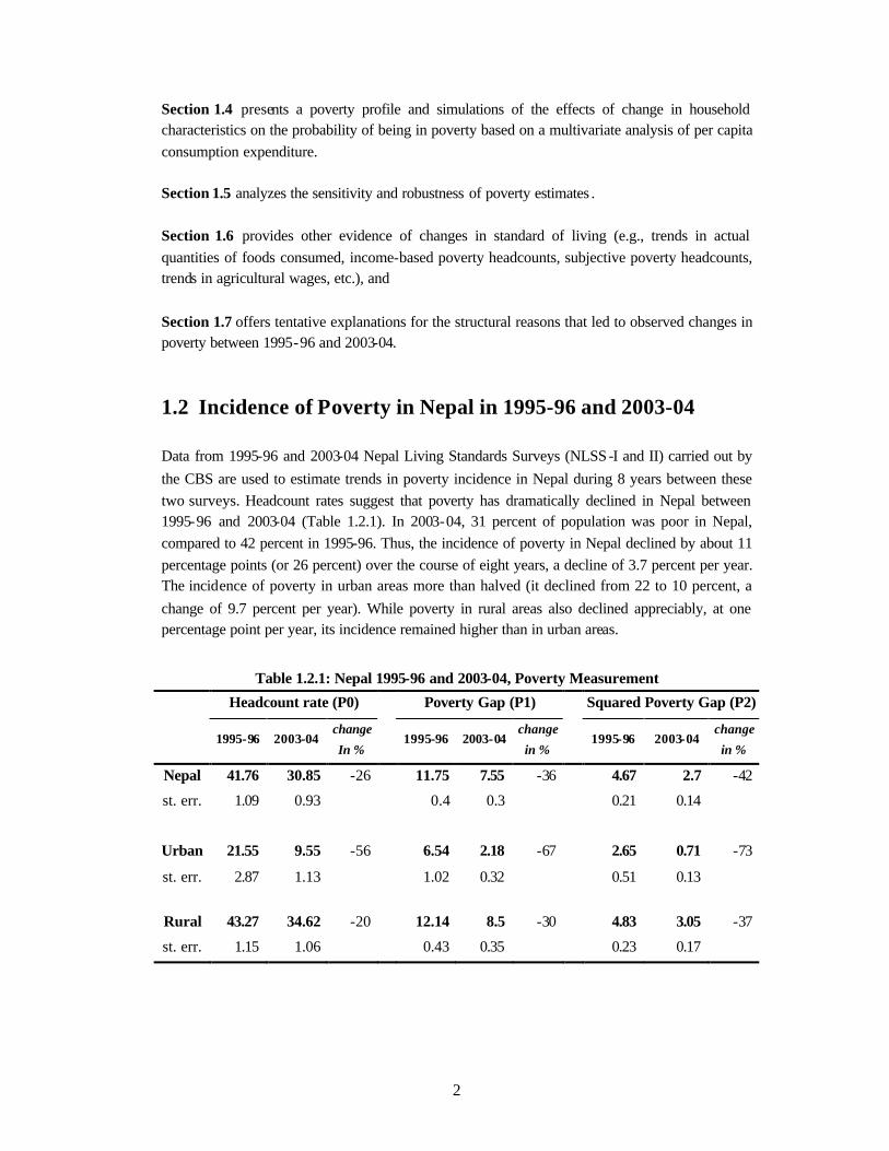
Data from 1995-96 and 2003-04 Nepal Living Standards Surveys (NLSS -I and II) carried out by the CBS are used to estimate trends in poverty incidence in Nepal during 8 years between these two surveys. Headcount rates suggest that poverty has dramatically declined in Nepal between 1995-96 and 2003-04 (Table 1.2.1). In 2003-04, 31 percent of population was poor in Nepal, compared to 42 percent in 1995-96. Thus, the incidence of poverty in Nepal declined by about 11 percentage points (or 26 percent) over the course of eight years, a decline of 3.7 percent per year. The incidence of poverty in urban areas more than halved (it declined from 22 to 10 percent, a change of 9.7 percent per year). While poverty in rural areas also declined appreciably, at one percentage point per year, its incidence remained higher than in urban areas.
Table 1.2.1: Nepal 1995-96 and 2003-04, Poverty Measurement
Headcount rate (P0) Poverty Gap (P1) Squared Poverty Gap (P2)
1995-96 2003-04 change
In % 1995-96 2003-04
change
in % 1995-96 2003-04
change
in %
Nepal 41.76 30.85 -26 11.75 7.55 -36 4.67 2.7 -42
st. err. 1.09 0.93 0.4 0.3 0.21 0.14
Urban 21.55 9.55 -56 6.54 2.18 -67 2.65 0.71 -73
st. err. 2.87 1.13 1.02 0.32 0.51 0.13
Rural 43.27 34.62 -20 12.14 8.5 -30 4.83 3.05 -37
st. err. 1.15 1.06 0.43 0.35 0.23 0.17
3
Box 1.1 Definition of Geographic Regions in Nepal Regions : “Kathmandu” comprises urban areas in the districts of Kathmandu, Lalitpur and Bhaktapur (together known as Kathmandu Valley); “Other urban” comprises all other urban areas – municipalities (cities and towns) - outside of the Kathmandu Valley; “rural Western Hills” includes Hills and Mountains from the Western, Mid-Western, and Far -Western Development regions; “rural Eastern Hills" refers to Hills and Mountains from the Eastern and Central Development Regions; “rural Western Terai” includes Terai belt from the Western, Mid-Western, and Far-Western Development regions; “rural Terai" refers to Terai area from the Eastern and Central Development Regions. Development regions: There are five east-to-west development regions: Eastern, Central, Western, Mid -Western and Far-Western regions. Belts: There are three north-to-south ecological belts: Mountains in the north (altitude 4877 to 8848 meters), Hills in the middle (altitude 610 to 4876 meters), and Terai in the South (up to 609 meters). Mountains region accounts for 35 percent of total land area of the country, while Hills and Terai 42 percent and 23 percent respectively.
The poverty gap (P1) estimates how far below the poverty line the poor are on average as a proportion of that line. The squared poverty gap (P2) takes into account not only the distance separating the poor from the poverty line, but also inequality among the poor, thereby giving more weight to the poorest people than the less poor. Trends in these measures mirror those observed with the headcount rates, but show an even faster decline (in percent terms). Both measures confirm that the incidence of urban poverty remained lower than that of rural poverty through-out the eight-year period; they also suggest that urban areas experienced greater reductions than rural areas in the depth and severity of poverty.
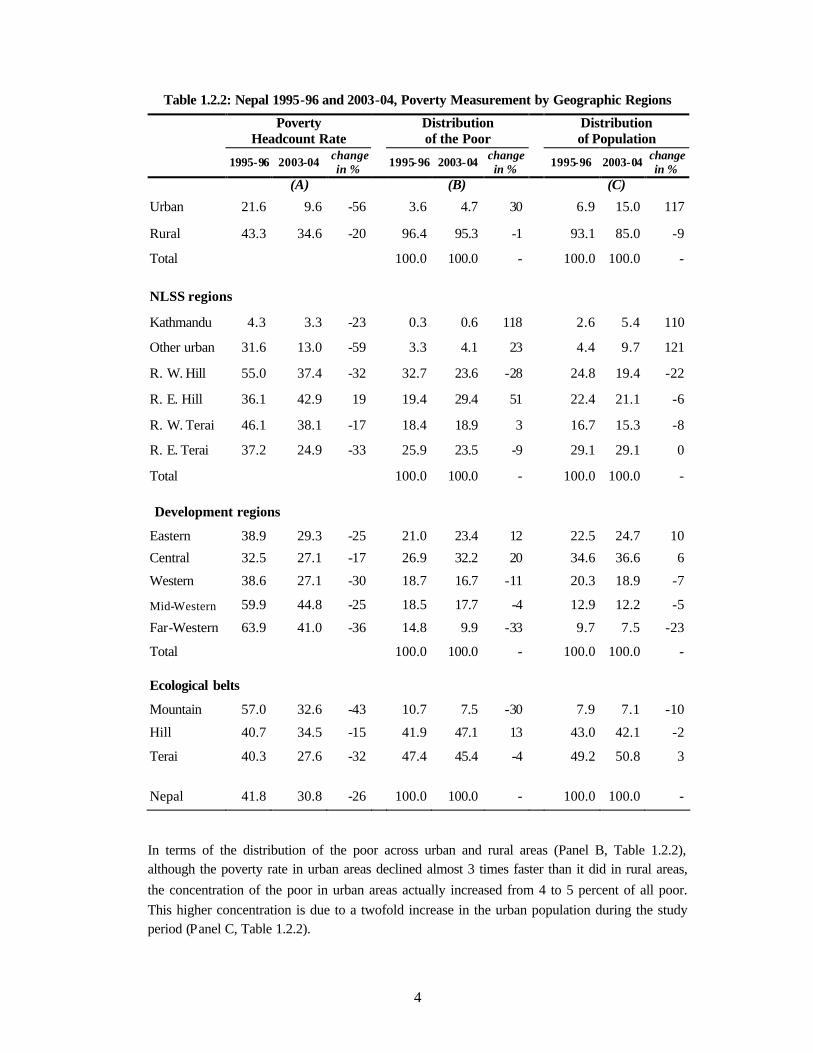
The incidence of poverty in 2003-04 varied considerably across different parts of the country, ranging from a low of 3.3 percent in Kathmandu to 42.9 percent in rural Eastern Hill and 38.1 percent in rural Western Terai (Panel A, Table 1.2.2). Between 1995-96 and 2003-04, poverty declined in both urban areas under consideration: in Kathmandu by 23 percent, and in “other urban” areas by 59 percent. In rural areas, the fastest decline in poverty occurred in rural Eastern Terai (33 percent) and rural Western Hills (32 percent). The incidence of poverty declined in rural Western Terai by 17 percent. By contrast, poverty in rural Eastern Hills increased from 36 to 43 percent. These changes affected the poverty rankings of the regions, with Eastern Hill undergoing the most dramatic shift, from having the third lowest incidence of poverty in 1995-96 to having the highest incidence in 2003-04.
Table 1.2.2 also shows that poverty rates declined across all development regions. At 27 percent, the Central and Western regions continued to have a poverty incidence below the national average in 2003-04, while the Mid- and Far -Western regions continued to be above the average (45 and 41 percent, respectively). In terms of poverty incidence across the belts of Nepal, the Terai belt has the lowest poverty rate at 28 percent, compared with 33 percent in the Mountains and 35 percent in the Hills.
4
Table 1.2.2: Nepal 1995-96 and 2003-04, Poverty Measurement by Geographic Regions
Poverty
Headcount Rate Distribution of the Poor Distribution
of Population
1995-96 2003-04 change in % 1995-96 2003-04 change
in % 1995-96 2003-04 change in %
(A) (B) (C)
Urban 21.6 9.6 -56 3.6 4.7 30 6.9 15.0 117
Rural 43.3 34.6 -20 96.4 95.3 -1 93.1 85.0 -9
Total 100.0 100.0 - 100.0 100.0 -
NLSS regions
Kathmandu 4.3 3.3 -23 0.3 0.6 118 2.6 5.4 110
Other urban 31.6 13.0 -59 3.3 4.1 23 4.4 9.7 121
R. W. Hill 55.0 37.4 -32 32.7 23.6 -28 24.8 19.4 -22
R. E. Hill 36.1 42.9 19 19.4 29.4 51 22.4 21.1 -6
R. W. Terai 46.1 38.1 -17 18.4 18.9 3 16.7 15.3 -8
R. E. Terai 37.2 24.9 -33 25.9 23.5 -9 29.1 29.1 0
Total 100.0 100.0 - 100.0 100.0 -
Development regions
Eastern 38.9 29.3 -25 21.0 23.4 12 22.5 24.7 10
Central 32.5 27.1 -17 26.9 32.2 20 34.6 36.6 6
Western 38.6 27.1 -30 18.7 16.7 -11 20.3 18.9 -7
Mid-Western 59.9 44.8 -25 18.5 17.7 -4 12.9 12.2 -5
Far-Western 63.9 41.0 -36 14.8 9.9 -33 9.7 7.5 -23
Total 100.0 100.0 - 100.0 100.0 -
Ecological belts
Mountain 57.0 32.6 -43 10.7 7.5 -30 7.9 7.1 -10
Hill 40.7 34.5 -15 41.9 47.1 13 43.0 42.1 -2
Terai 40.3 27.6 -32 47.4 45.4 -4 49.2 50.8 3 Nepal 41.8 30.8 -26 100.0 100.0 - 100.0 100.0 -
In terms of the distribution of the poor across urban and rural areas (Panel B, Table 1.2.2), although the poverty rate in urban areas declined almost 3 times faster than it did in rural areas, the concentration of the poor in urban areas actually increased from 4 to 5 percent of all poor. This higher concentration is due to a twofold increase in the urban population during the study period (Panel C, Table 1.2.2).
5
In 2003-04 the largest share (29 percent) of the total number of poor people in Nepal resided in rural Eastern Hill. This is an appreciable change from 1995-96, when rural Western Hill housed a third of all poor, the highest concentration in that year. Both a rapid reduction in rural Western Hill’s headcount poverty rate and a significant reduction in the proportion of the population residing there contributed to the region’s change in ranking.
In terms of the distribution of the poor across development regions, the Central region continues to house the greatest number of poor Nepalese, while having a poverty incidence below the national average. The Mid-Western and Far-Western regions have the highest levels of poverty, 45 and 41 percent, respectively, but, on the account of low population density, house only 18 and 10 percent of all poor, respectively. In terms of the distribution of the poor across the belts, the Hills and Terai have roughly similar proportions of poor people – 47 and 45 percent, respectively – with the Mountains accounting for 8 percent.
1.3 Growth and Inequality: Changes between 1995-96 and 2003 -04
Poverty measures provide a summary of the distribution of welfare, but a richer analysis of the data is possible while analyzing the entire distribution. In this section, we examine trends in NLSS-based real consumption, compare NLSS and National Accounts-based trends, and analyze trends in inequality. To gain further insights into the relationship between growth, poverty, and inequality we consider a range of growth-inequality and inter-intra regional decompositions.
1.3.1 Trends in Real Expenditure
As mentioned above, we use the implied poverty line deflators (ratios of regional poverty lines) to express the NLSS-II consumption aggregates in 1995-96 average Nepal prices. All subsequent references in this note to real per -capita expenditure (PCE) refer to nominal expenditures divided by these price indices.2
Table 1.3.1 presents trends in real PCE. A number of observations emerge:
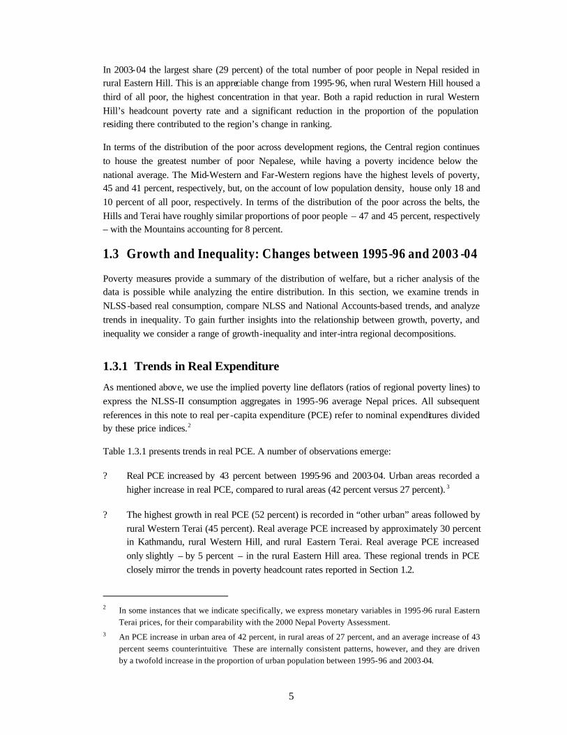
? Real PCE increased by 43 percent between 1995-96 and 2003-04. Urban areas recorded a higher increase in real PCE, compared to rural areas (42 percent versus 27 percent). 3
? The highest growth in real PCE (52 percent) is recorded in “other urban” areas followed by rural Western Terai (45 percent). Real average PCE increased by approximately 30 percent in Kathmandu, rural Western Hill, and rural Eastern Terai. Real average PCE increased only slightly – by 5 percent – in the rural Eastern Hill area. These regional trends in PCE closely mirror the trends in poverty headcount rates reported in Section 1.2.
2 In some instances that we indicate specifically, we express monetary variables in 1995-96 rural Eastern
Terai prices, for their comparability with the 2000 Nepal Poverty Assessment. 3 An PCE increase in urban area of 42 percent, in rural areas of 27 percent, and an average increase of 43
percent seems counterintuitive. These are internally consistent patterns, however, and they are driven by a twofold increase in the proportion of urban population between 1995-96 and 2003-04.

6
? Real PCE increased for all quintiles, but much more so for the higher expenditure groups. Per capita consumption of the bottom three quintiles increased by less than 3 percent per year, while that of the population in the highest quintiles increased by 3.7 and 6.4 percent per year. While the growth in per capita consumption of the poorer population is more than “respectable,” the growth in consumption of the richer population is remarkably high. These patterns indicate a sharp increase in inequality.
Table 1.3.1: Nepal 1995-96 and 2003-04, Distribution of Real (1995-96 Average Nepal Prices) Per-Capita Expenditure
Real Mean Per-Capita Expenditure (NRS per year)
Change (in percent)
1995-96 2003-2004 over 8 year period
annual
Kathmandu 20,130 26,832 33 3.66
Other urban 11,309 17,229 52 5.4
R. Western Hill 5,953 7,774 31 3.39
R. Eastern Hill 7,447 7,812 5 0.6
R. Western Terai 6,190 8,976 45 4.76
R. Eastern Terai 7,034 9,225 31 3.45
Urban 14,536 20,633 42 4.48
Rural 6,694 8,499 27 3.03 1 (Lowest quintile) 2,898 3,524 22 2.47
2 4,347 5,186 19 2.23
3 5,687 7,121 25 2.85
4 7,683 10,255 33 3.68
5 (Highest quintile) 15,477 25,387 64 6.38
Nepal 7,235 10,318 43 4.54
Note: Outliers, 0.5 percentile at each tail of the distribution, excluded.
How do the trends in the PCE measured in the NLSS series relate to the trends in GDP and private consumption measured in the National Accounts Statistics? Table 1.3.2 compares these statistics in both nominal and real terms.
7
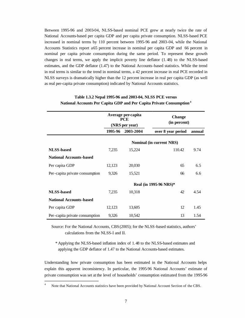
Between 1995-96 and 2003-04, NLSS-based nominal PCE grew at nearly twice the rate of National Accounts-based per capita GDP and per capita private consumption. NLSS-based PCE increased in nominal terms by 110 percent between 1995-96 and 2003-04, while the National Accounts Statistics report a 65 percent increase in nominal per capita GDP and 66 percent in nominal per capita private consumption during the same period. To represent these growth changes in real terms, we apply the implicit poverty line deflator (1. 48) to the NLSS-based estimates, and the GDP deflator (1.47) to the National Accounts-based statistics. While the trend in real terms is similar to the trend in nominal terms, a 42 percent increase in real PCE recorded in NLSS surveys is dramatically higher than the 12 percent increase in real per capita GDP (as well as real per-capita private consumption) indicated by National Accounts statistics.
Table 1.3.2 Nepal 1995-96 and 2003-04, NLSS PCE versus National Accounts Per Capita GDP and Per Capita Private Consumption 4
Average per-capita PCE
(NRS per year)
Change (in percent)
1995-96 2003-2004 over 8 year period annual
Nominal (in current NRS)
NLSS-based 7,235 15,224 110.42 9.74
National Accounts-based
Per capita GDP 12,123 20,030 65 6.5
Per-capita private consumption 9,326 15,521 66 6.6
Real (in 1995-96 NRS)*
NLSS-based 7,235 10,318 42 4.54
National Accounts-based
Per capita GDP 12,123 13,605 12 1.45
Per-capita private consumption 9,326 10,542 13 1.54
Source: For the National Accounts, CBS (2005); for the NLSS-based statistics, authors’ calculations from the NLSS-I and II.
* Applying the NLSS-based inflation index of 1.48 to the NLSS-based estimates and applying the GDP deflator of 1.47 to the National Accounts-based estimates.
Understanding how private consumption has been estimated in the National Accounts helps explain this apparent inconsistency. In particular, the 1995-96 National Accounts’ estimate of private consumption was set at the level of households’ consumption estimated from the 1995-96 4 Note that National Accounts statistics have been provided by National Account Section of the CBS.
8
NLSS with a upward adjustment to account for (i) home-produced non-food goods such as self-produced clothing, amenities, furniture, utensils, etc. that were not covered in the NLSS, (ii) in-
kind transfers from the government to households such as textbooks, medicine, etc. that are not captured in NLSS, and (iii) the private consumption of resident foreign households that are not
covered by NLSS. There are no estimates of disposable income in Nepal and therefore, is not
directly comparable with the survey-based estimates.
Comparing GDP growth rate with NLSS-based consumption growth rate is also problematic since GDP does not accurately approximate personal income and personal consumption in an economy
with a large inflow of remittances from abroad. 5 FY03 remittance transfer through official channels alone totaled about NRS 54 billion, equivalent to 12.4 percent of GDP, compared to its share of less than 5 percent eight years ago. The gross national income (GNI) growth series does not fully capture the growth in private consumption associated with remittances either, because
wages of workers who have been outside of the country for one year or longer are not counted as
national income, but rather as national savings. There are no details of independently derived estimates of national savings in Nepal.
1.3.2 The Relationship between Growth in Per-capita Expenditure and Poverty
Real PCE grew by an estimated 43 percent, while poverty declined by 26 percent, during the 8 years between the two NLSS surveys. This implies that total elasticity of poverty reduction with respect to growth has been negative 0.6, i.e., every percent in growth of PCE resulted in 0.6
percent reduction in the proportion of the poor. The corresponding estimate for the growth-
poverty-reduction elasticity is 1.33 for urban areas (where a 42 percent growth in PCE was accompanied by a 56 percent reduction in poverty). In rural areas the estimate is 0.74 (a 27
percent growth in PCE accompanied by a 20 percent reduction in poverty).
These elasticities of poverty reduction with respect to growth are quite low by international standards. Specifically, Ravallion 20006 places cross-national estimates of poverty reduction with
respect to growth at around negative 2, ind icating that for every 1 percent increase in the mean income, on average, poverty is reduced by 2 percent.
5 Leaving out remittances did not impact estimates of private consumption in the 1995-96 National
Accounts as much as it did the 2003 -04 estimates because while a substantial amount of remittances were coming into the country during the early and mid 1990s, growth in remittances really picked up in the late 1990s.
6 Ravallion, Martin (2000) “Growth, Inequality and Poverty: Looking beyond Averages.”
9
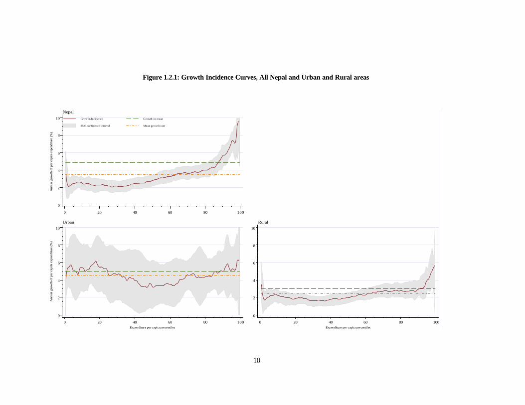
1.3.3 Growth Incidence Curves
To further answer the question of how the gains from aggregate growth were distributed in relation to the initial PCE we calculate the growth-incidence curves (GICs) (see Ravallion and
Chen, 2003).7 Growth incidence curves are constructed by plotting the annualized rate of growth at percentiles of PCE distribution, allowing for further insight on the patterns of growth between
the two surveys. Figure 1.2.1 presents GICs calculated for all of Nepal, as well as for urban and
rural areas separately.
Real PCE increased for all deciles in both urban and rural areas, but this increase was skewed toward urban areas and higher expenditure groups. While urban growth was equally distributed
across the lower and upper halves of the distribution, in rural areas growth was higher among high-income households. These patterns help account for the patterns of poverty decline (higher in urban areas and lower in rural areas) reported in Table 1.2.1. 8
Similarly, GICs at the regional level help explain regional patterns of poverty decline. Presented in Annex 1, Figure A1.1, they show that growth in real per-capita expenditure of the lower percentiles in “other urban” areas and in rural Western Hill was considerably higher than that of the upper percentiles. In rural Eastern Hill growth was uniformly low, with the exception of the
very top percentiles. The western part of rural Terai had uniform growth, except for the very top
percentiles, which grew faster. In eastern rural Terai the entire upper part of the distribution grew faster than the lower part.
7 See Ravallion, Martin and Shaohua Chen (2003), “Measuring Pro-Poor Growth”, Economics Letters ,
Vol. 78(1): 93-99. 8 Figure 2.1 indicates that growth at the upper percentiles of the distribution in Nepal overall is actually
higher than either growth in urban or rural areas taken separately. This pattern is driven by an increase in the proportion of the population living in urban areas. It is straightforward to work out an arithmetic example of non -additive growth rates between two sectors, between two time periods, when a population shares in the sectors change.
10
Figure 1.2.1: Growth Incidence Curves, All Nepal and Urban and Rural areas
0
2
4
6
8
10
Ann
ual g
row
th o
f per
cap
ita e
xpen
ditu
re (%
)
0 20 40 60 80 100
Growth-Incidence Growth in mean
95% confidence interval Mean growth rate
Nepal
0
2
4
6
8
10
Ann
ual g
row
th o
f per
cap
ita e
xpen
ditu
re (%
)
0 20 40 60 80 100Expenditure per capita percentiles
Urban
0
2
4
6
8
10
0 20 40 60 80 100Expenditure per capita percentiles
Rural
11
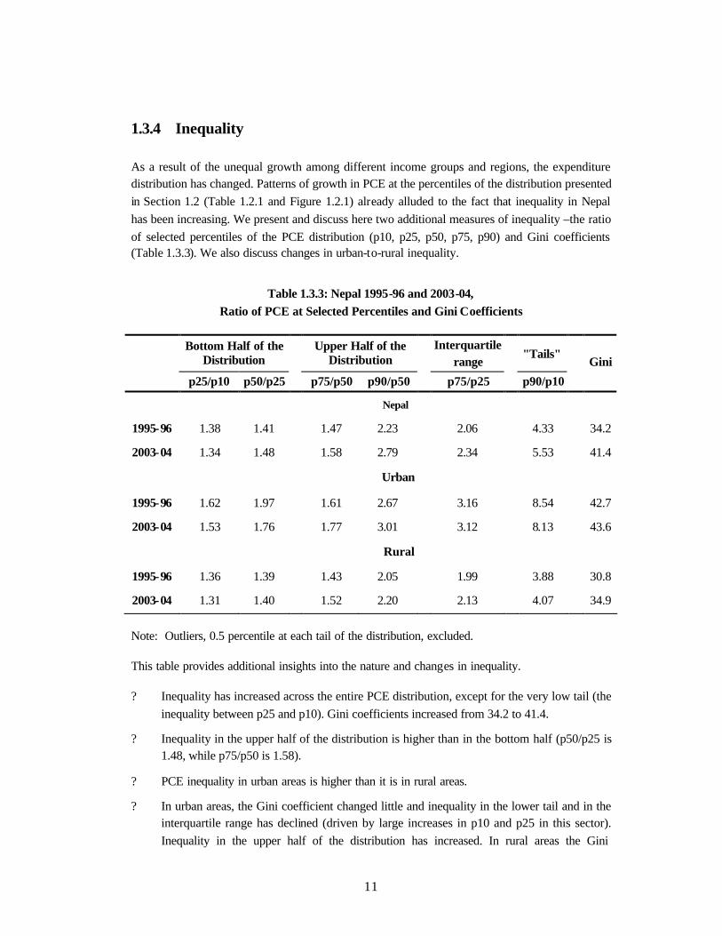
1.3.4 Inequality
As a result of the unequal growth among different income groups and regions, the expenditure distribution has changed. Patterns of growth in PCE at the percentiles of the distribution presented in Section 1.2 (Table 1.2.1 and Figure 1.2.1) already alluded to the fact that inequality in Nepal has been increasing. We present and discuss here two additional measures of inequality –the ratio of selected percentiles of the PCE distribution (p10, p25, p50, p75, p90) and Gini coefficients (Table 1.3.3). We also discuss changes in urban-to-rural inequality.
Table 1.3.3: Nepal 1995-96 and 2003-04, Ratio of PCE at Selected Percentiles and Gini Coefficients
Bottom Half of the Distribution
Upper Half of the Distribution
Interquartile range
"Tails"
p25/p10 p50/p25 p75/p50 p90/p50 p75/p25 p90/p10
Gini
Nepal
1995-96 1.38 1.41 1.47 2.23 2.06 4.33 34.2
2003-04 1.34 1.48 1.58 2.79 2.34 5.53 41.4
Urban
1995-96 1.62 1.97 1.61 2.67 3.16 8.54 42.7
2003-04 1.53 1.76 1.77 3.01 3.12 8.13 43.6
Rural
1995-96 1.36 1.39 1.43 2.05 1.99 3.88 30.8
2003-04 1.31 1.40 1.52 2.20 2.13 4.07 34.9
Note: Outliers, 0.5 percentile at each tail of the distribution, excluded.
This table provides additional insights into the nature and changes in inequality.
? Inequality has increased across the entire PCE distribution, except for the very low tail (the inequality between p25 and p10). Gini coefficients increased from 34.2 to 41.4.
? Inequality in the upper half of the distribution is higher than in the bottom half (p50/p25 is 1.48, while p75/p50 is 1.58).
? PCE inequality in urban areas is higher than it is in rural areas.
? In urban areas, the Gini coefficient changed little and inequality in the lower tail and in the interquartile range has declined (driven by large increases in p10 and p25 in this sector). Inequality in the upper half of the distribution has increased. In rural areas the Gini
12
coefficient increased, and inequality has increased in all except the very low part of the distribution.
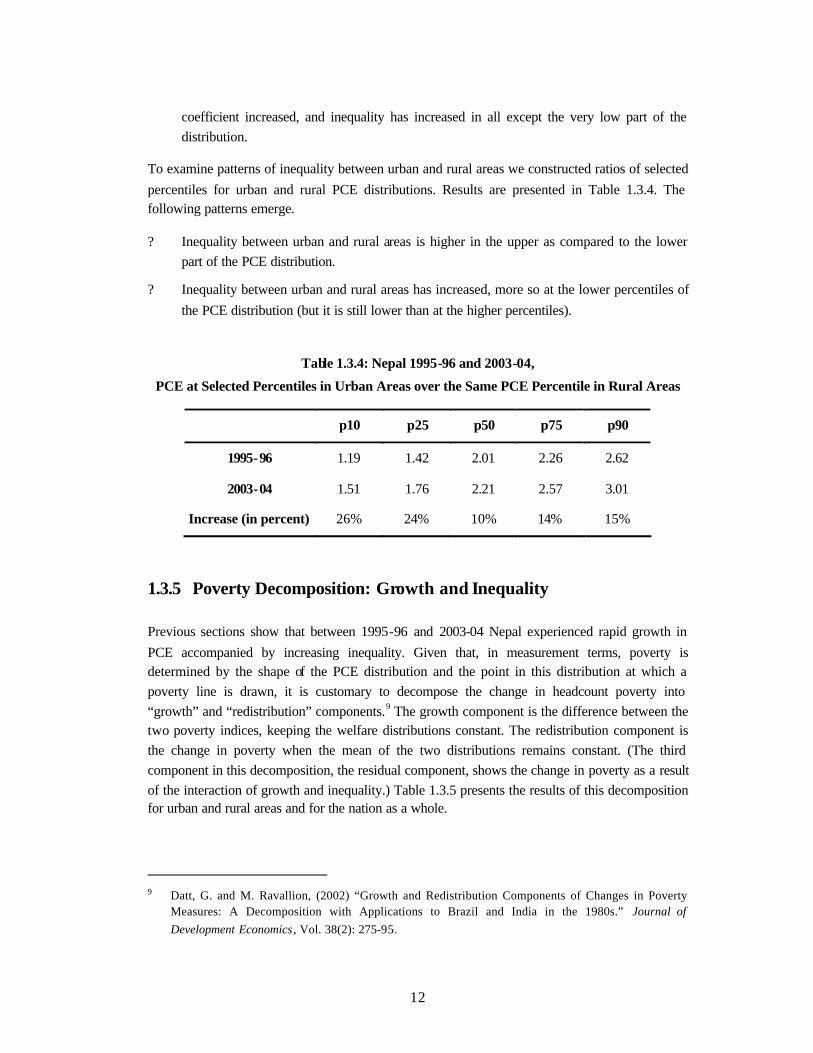
To examine patterns of inequality between urban and rural areas we constructed ratios of selected percentiles for urban and rural PCE distributions. Results are presented in Table 1.3.4. The following patterns emerge.
? Inequality between urban and rural areas is higher in the upper as compared to the lower part of the PCE distribution.
? Inequality between urban and rural areas has increased, more so at the lower percentiles of the PCE distribution (but it is still lower than at the higher percentiles).
Table 1.3.4: Nepal 1995-96 and 2003-04,
PCE at Selected Percentiles in Urban Areas over the Same PCE Percentile in Rural Areas
p10 p25 p50 p75 p90
1995-96 1.19 1.42 2.01 2.26 2.62
2003-04 1.51 1.76 2.21 2.57 3.01
Increase (in percent) 26% 24% 10% 14% 15%
1.3.5 Poverty Decomposition: Growth and Inequality
Previous sections show that between 1995-96 and 2003-04 Nepal experienced rapid growth in PCE accompanied by increasing inequality. Given that, in measurement terms, poverty is determined by the shape of the PCE distribution and the point in this distribution at which a poverty line is drawn, it is customary to decompose the change in headcount poverty into “growth” and “redistribution” components.9 The growth component is the difference between the two poverty indices, keeping the welfare distributions constant. The redistribution component is the change in poverty when the mean of the two distributions remains constant. (The third component in this decomposition, the residual component, shows the change in poverty as a result of the interaction of growth and inequality.) Table 1.3.5 presents the results of this decomposition for urban and rural areas and for the nation as a whole.
9 Datt, G. and M. Ravallion, (2002) “Growth and Redistribution Components of Changes in Poverty
Measures: A Decomposition with Applications to Brazil and India in the 1980s.” Journal of Development Economics , Vol. 38(2): 275-95.
13
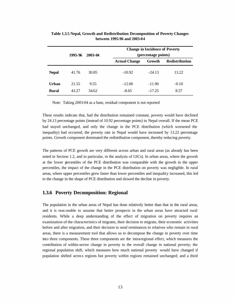
Table 1.3.5 Nepal, Growth and Redistribution Decomposition of Poverty Changes between 1995-96 and 2003-04
Change in Incidence of Poverty (percentage points)
1995-96 2003-04
Actual Change Growth Redistribution
Nepal 41.76 30.85 -10.92 -24.13 13.22 Urban 21.55 9.55 -12.00 -11.90 -0.10
Rural 43.27 34.62 -8.65 -17.25 8.57
Note: Taking 2003-04 as a base, residual component is not reported
These results indicate that, had the distribution remained constant, poverty would have declined by 24.13 percentage points (instead of 10.92 percentage points) in Nepal overall. If the mean PCE had stayed unchanged, and only the change in the PCE distribution (which worsened the inequality) had occurred, the poverty rate in Nepal would have increased by 13.22 percentage points. Growth component dominated the redistribution component, thereby reducing poverty.
The patterns of PCE growth are very different across urban and rural areas (as already has been noted in Section 1.2, and in particular, in the analysis of GICs). In urban areas, where the growth at the lower percentiles of the PCE distribution was comparable with the growth in the upper percentiles, the impact of the change in the PCE distribution on poverty was negligible. In rural areas, where upper percentiles grew faster than lower percentiles and inequality increased, this led to the change in the shape of PCE distribution and slowed the decline in poverty.
1.3.6 Poverty Decomposition: Regional
The population in the urban areas of Nepal has done relatively better than that in the rural areas, and it is reas onable to assume that better prospects in the urban areas have attracted rural residents. While a deep understanding of the effect of migration on poverty requires an examination of the characteristics of migrants, their decision to migrate, their economic activities before and after migration, and their decision to send remittances to relatives who remain in rural areas, there is a measurement tool that allows us to decompose the change in poverty over time into three components. These three components are the intra-regional effect, which measures the contribution of within-sector change in poverty to the overall change in national poverty; the regional population shift, which measures how much national poverty would have changed if population shifted acros s regions but poverty within regions remained unchanged; and a third
14
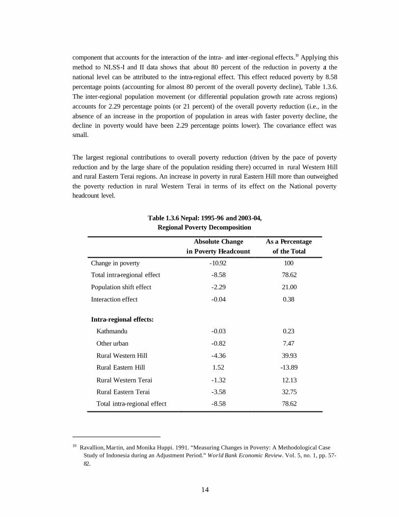
component that accounts for the interaction of the intra- and inter-regional effects.10 Applying this method to NLSS-I and II data shows that about 80 percent of the reduction in poverty at the national level can be attributed to the intra-regional effect. This effect reduced poverty by 8.58 percentage points (accounting for almost 80 percent of the overall poverty decline), Table 1.3.6. The inter-regional population movement (or differential population growth rate across regions) accounts for 2.29 percentage points (or 21 percent) of the overall poverty reduction (i.e., in the absence of an increase in the proportion of population in areas with faster poverty decline, the decline in poverty would have been 2.29 percentage points lower). The covariance effect was small.
The largest regional contributions to overall poverty reduction (driven by the pace of poverty reduction and by the large share of the population residing there) occurred in rural Western Hill and rural Eastern Terai regions. An increase in poverty in rural Eastern Hill more than outweighed the poverty reduction in rural Western Terai in terms of its effect on the National poverty headcount level.
Table 1.3.6 Nepal: 1995-96 and 2003-04, Regional Poverty Decomposition
Absolute Change
in Poverty Headcount As a Percentage
of the Total
Change in poverty -10.92 100
Total intra-regional effect -8.58 78.62
Population shift effect -2.29 21.00
Interaction effect -0.04 0.38
Intra-regional effects:
Kathmandu -0.03 0.23
Other urban -0.82 7.47
Rural Western Hill -4.36 39.93
Rural Eastern Hill 1.52 -13.89
Rural Western Terai -1.32 12.13
Rural Eastern Terai -3.58 32.75
Total intra-regional effect -8.58 78.62
10 Ravallion, Martin, and Monika Huppi. 1991. “Measuring Changes in Poverty: A Methodological Case
Study of Indonesia during an Adjustment Period.” World Bank Economic Review. Vol. 5, no. 1, pp. 57-82.
15
1.4 Poverty Profile and Multivariate Analysis of Poverty
Both NLSS-I and II contain extensive modules on various characteristics of households – demographic composition, housing situation, access to facilities, sector of employment of adult household members, education attainments, etc. The results of both surveys have been published, see “Nepal Living Standards Survey Report 1996” Volumes 1 and 2 for the NLSS-I results and “Nepal Living Standards Survey 2004” Volumes 1 and 2 for NLSS-II results as well as for comparison of trends in selected indicators between 1995-96 and 2003-04. This section uses these data together with information on poverty status of households to estimate poverty rates across households with different characteristics.
1.4.1 Poverty Profile
A poverty profile describes who the poor are by indicating the probability of being poor according to various characteristics, such as the sector of employment and the level of education of the household head, the demographic composition of a household (i.e., household size, number of children, caste-ethnic status), and the amount of land a household possesses. This section provides a profile of the poor with respect to the above-mentioned characteristics.
Sector of employment of the household head
Households headed by agricultural wage laborers are the poorest in Nepal. In 1995-96 the incidence of poverty among this group was almost 56 percent and it declined only slightly to 54 percent in 2003-04. As a share of the national population this group is small and in decline. Comprising 12 percent of the population and 16 percent of the poor in 1995-96, in 2003-04 this group made up 6 percent of the total population and 11 percent of all poor.
The second poorest group in Nepal is made up of those who live in households headed by self-employed in agriculture. Unlike agricultural wage households, this group experienced a substantial decline in poverty from 43 to 33 percent between 1995-96 and 2003-04. This is the most populated employment sector category with 67 percent of all poor in 2003-04 falling to this category.
Households whose heads’ main occupation is in trade and services experienced a dramatic decline in poverty between 1995-96 and 2003-04, and had a relatively low incidence of poverty (11 and 14 percent, respectively) in 2003-04.
16
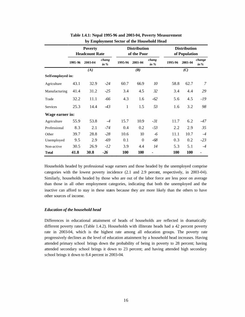
Table 1.4.1: Nepal 1995-96 and 2003-04, Poverty Measurement by Employment Sector of the Household Head
Poverty
Headcount Rate Distribution
of the Poor Distribution
of Population
1995-96 2003-04 chang in % 1995-96 2003-04
chang in % 1995-96 2003-04
change in %
(A) (B) (C)
Self-employed in:
Agriculture 43.1 32.9 -24 60.7 66.9 10 58.8 62.7 7
Manufacturing 41.4 31.2 -25 3.4 4.5 32 3.4 4.4 29
Trade 32.2 11.1 -66 4.3 1.6 -62 5.6 4.5 -19
Services 25.3 14.4 -43 1 1.5 53 1.6 3.2 98
Wage earner in:
Agriculture 55.9 53.8 -4 15.7 10.9 -31 11.7 6.2 -47
Professional 8.3 2.1 -74 0.4 0.2 -53 2.2 2.9 35 Other 39.7 28.8 -28 10.6 10 -6 11.1 10.7 -4 Unemployed 9.5 2.9 -69 0.1 0 -68 0.3 0.2 -23 Non-active 30.5 26.9 -12 3.9 4.4 14 5.3 5.1 -4 Total 41.8 30.8 -26 100 100 - 100 100 -
Households headed by professional wage earners and those headed by the unemployed comprise categories with the lowest poverty incidence (2.1 and 2.9 percent, respectively, in 2003-04). Similarly, households headed by those who are out of the labor force are less poor on average than those in all other employment categories, indicating that both the unemployed and the inactive can afford to stay in these states because they are more likely than the others to have other sources of income.
Education of the household head
Differences in educational attainment of heads of households are reflected in dramatically different poverty rates (Table 1.4.2). Households with illiterate heads had a 42 percent poverty rate in 2003-04, which is the highest rate among all education groups. The poverty rate progressively declines as the level of education attainment by a household head increases. Having attended primary school brings down the probability of being in poverty to 28 percent; having attended secondary school brings it down to 23 percent; and having attended high secondary school brings it down to 8.4 percent in 2003-04.
17
Box 1.4.1: Proportion of Households Receiving Remittances by the Household Heads’ Age and S ex
1995-96 2003-04
Male 25 year or younger 18.99 20.67
Male 26-45 years old 14.58 13.86
Male 46 years and older 22.52 32.17
Female-headed 55.43 65.42
Total 23.43 31.92
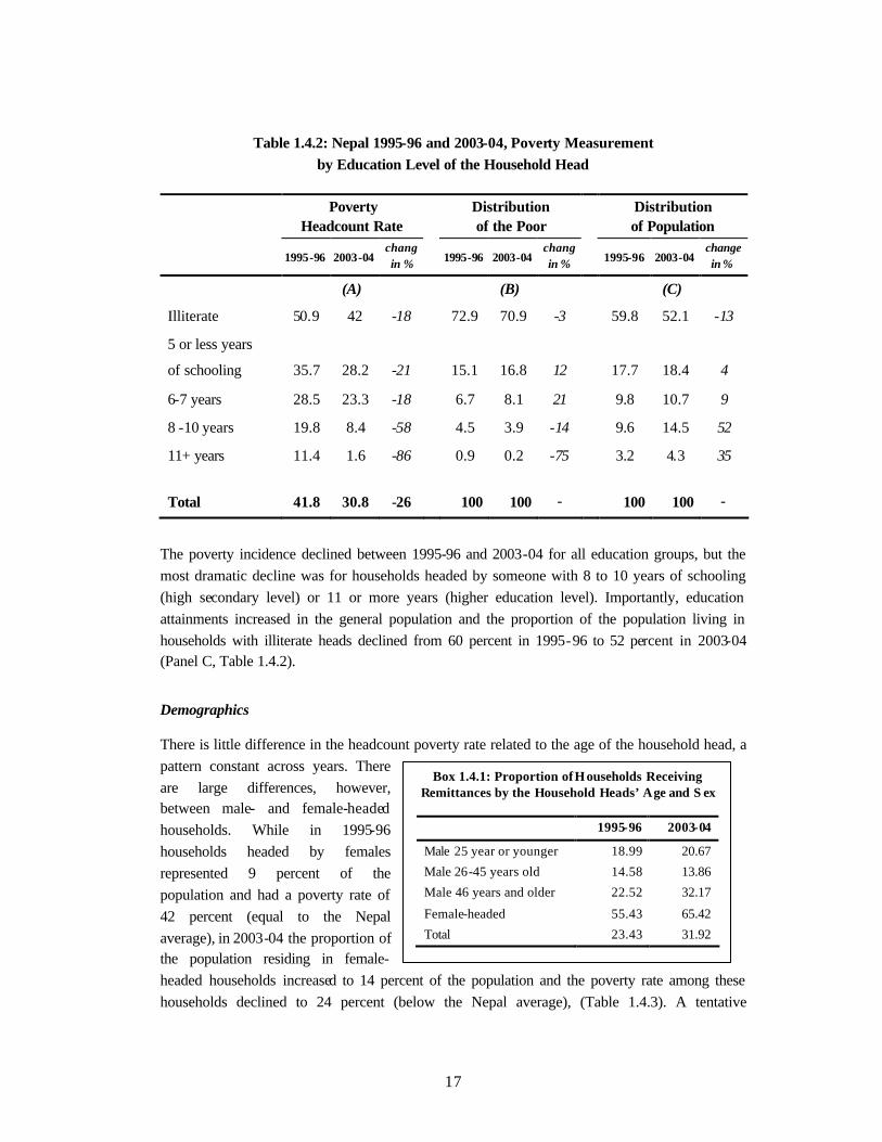
Table 1.4.2: Nepal 1995-96 and 2003-04, Poverty Measurement by Education Level of the Household Head
Poverty
Headcount Rate Distribution
of the Poor Distribution
of Population
1995-96 2003-04 chang in % 1995-96 2003-04
chang in % 1995-96 2003-04
change in %
(A) (B) (C)
Illiterate 50.9 42 -18 72.9 70.9 -3 59.8 52.1 -13
5 or less years
of schooling 35.7 28.2 -21
15.1 16.8 12 17.7 18.4 4
6-7 years 28.5 23.3 -18 6.7 8.1 21 9.8 10.7 9
8 -10 years 19.8 8.4 -58 4.5 3.9 -14 9.6 14.5 52
11+ years 11.4 1.6 -86 0.9 0.2 -75 3.2 4.3 35
Total 41.8 30.8 -26 100 100 - 100 100 -
The poverty incidence declined between 1995-96 and 2003-04 for all education groups, but the most dramatic decline was for households headed by someone with 8 to 10 years of schooling (high secondary level) or 11 or more years (higher education level). Importantly, education attainments increased in the general population and the proportion of the population living in households with illiterate heads declined from 60 percent in 1995-96 to 52 percent in 2003-04 (Panel C, Table 1.4.2).
Demographics
There is little difference in the headcount poverty rate related to the age of the household head, a pattern constant across years. There are large differences, however, between male- and female-headed households. While in 1995-96 households headed by females represented 9 percent of the population and had a poverty rate of 42 percent (equal to the Nepal average), in 2003-04 the proportion of the population residing in female-headed households increased to 14 percent of the population and the poverty rate among these households declined to 24 percent (below the Nepal average), (Table 1.4.3). A tentative

18
explanation for this pattern is that households headed by females tend to have a main breadwinner working elsewhere who supports the household by sending remittances (Box 1.4.2).
Table 1.4.3: Nepal 1995-96 and 2003-04 Poverty Measurement by HH Head’s Age and Sex
Poverty
Headcount Rate Distribution
of the Poor Distribution
of Population
1995-96 2003-04 chang in %
1995-96 2003-04 chang in %
1995-96 2003-04 change in %
(A) (B) (C)
Male 25 year or younger 40.5 32.5 -20 5 3.5 -30 5.1 3.3 -35.4
Male 26-45 years old
43.8 32.5 -26 41.5 37.9 -9 39.6 35.9 -9.3
Male 46 years and older
40.2 31.6 -21 45 47.6 6 46.7 46.4 -0.8
Female-headed 41.6 23.8 -43 8.5 11.1 31 8.5 14.4 68.8
Total 41.8 30.8 -26 100 100 - 100 100 -
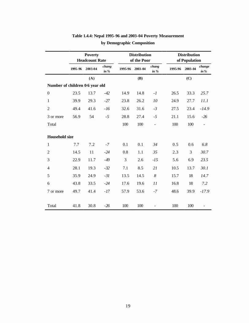
Both an increase in the number of small children and an increase in the number of household members are related to an increase in the poverty headcount rate (Table 1.4.4). The higher level of poverty headcount in larger households or households with more children is, at least in part, related to the fact that the definition of poverty line for Nepal does not incorporate economies of
scale. However, the pattern of slower-than-average poverty reduction rate among households with
2 or more small children or 6 or more family members may attest to structural factors that prevent these households from escaping pover ty.
The proportion of the population living in households with 7 or more members has declined from
almost 50 to 40 percent (Panel C, Table 1.4.4). Given that these households have the highest incidence of poverty of all households both in 1995-96 and 2003-04, this development may have
contributed to the overall poverty decline.
19
Table 1.4.4: Nepal 1995-96 and 2003-04 Poverty Measurement
by Demographic Composition
Poverty
Headcount Rate Distribution
of the Poor Distribution
of Population
1995-96 2003-04 chang in %
1995-96 2003-04 chang in %
1995-96 2003-04 change in %
(A) (B) (C)
Number of children 0-6 year old
0 23.5 13.7 -42 14.9 14.8 -1 26.5 33.3 25.7
1 39.9 29.3 -27 23.8 26.2 10 24.9 27.7 11.1
2 49.4 41.6 -16 32.6 31.6 -3 27.5 23.4 -14.9
3 or more 56.9 54 -5 28.8 27.4 -5 21.1 15.6 -26
Total 100 100 - 100 100 -
Household size
1 7.7 7.2 -7 0.1 0.1 34 0.5 0.6 6.8
2 14.5 11 -24 0.8 1.1 35 2.3 3 30.7
3 22.9 11.7 -49 3 2.6 -15 5.6 6.9 23.5
4 28.1 19.3 -32 7.1 8.5 21 10.5 13.7 30.1
5 35.9 24.9 -31 13.5 14.5 8 15.7 18 14.7
6 43.8 33.5 -24 17.6 19.6 11 16.8 18 7.2
7 or more 49.7 41.4 -17 57.9 53.6 -7 48.6 39.9 -17.9
Total 41.8 30.8 -26 100 100 - 100 100 -
20
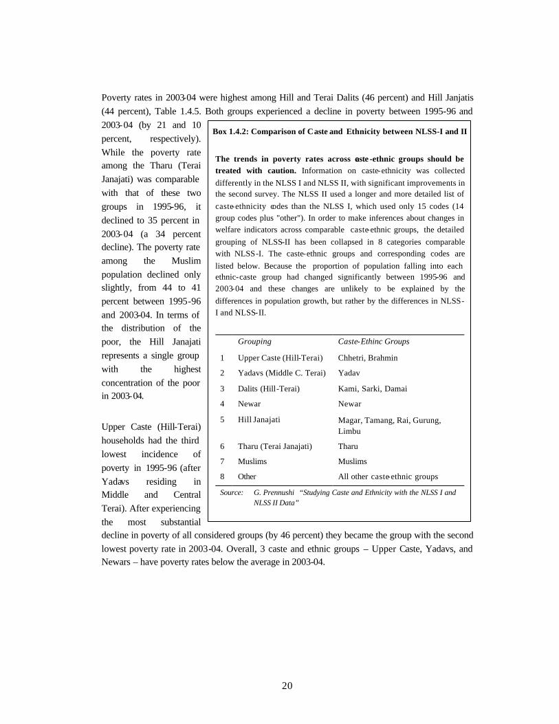
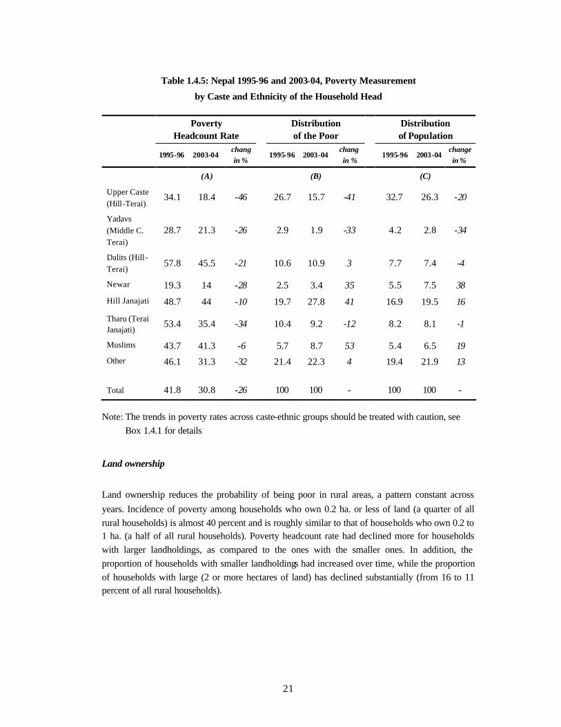
Poverty rates in 2003-04 were highest among Hill and Terai Dalits (46 percent) and Hill Janjatis (44 percent), Table 1.4.5. Both groups experienced a decline in poverty between 1995-96 and 2003-04 (by 21 and 10 percent, respectively). While the poverty rate among the Tharu (Terai Janajati) was comparable with that of these two groups in 1995-96, it declined to 35 percent in 2003-04 (a 34 percent decline). The poverty rate among the Muslim population declined only slightly, from 44 to 41 percent between 1995-96 and 2003-04. In terms of the distribution of the poor, the Hill Janajati represents a single group with the highest concentration of the poor in 2003-04.
Upper Caste (Hill-Terai) households had the third lowest incidence of poverty in 1995-96 (after Yadavs residing in Middle and Central Terai). After experiencing the most substantial decline in poverty of all considered groups (by 46 percent) they became the group with the second lowest poverty rate in 2003-04. Overall, 3 caste and ethnic groups – Upper Caste, Yadavs, and Newars – have poverty rates below the average in 2003-04.
Box 1.4.2: Comparison of Caste and Ethnicity between NLSS-I and II
The trends in poverty rates across caste -ethnic groups should be treated with caution. Information on caste-ethnicity was collected differently in the NLSS I and NLSS II, with significant improvements in the second survey. The NLSS II used a longer and more detailed list of caste-ethnicity codes than the NLSS I, which used only 15 codes (14 group codes plus "other"). In order to make inferences about changes in welfare indicators across comparable caste-ethnic groups, the detailed grouping of NLSS-II has been collapsed in 8 categories comparable with NLSS-I. The caste-ethnic groups and corresponding codes are listed below. Because the proportion of population falling into each ethnic-caste group had changed significantly between 1995-96 and 2003-04 and these changes are unlikely to be explained by the differences in population growth, but rather by the differences in NLSS-I and NLSS-II.
Grouping Caste-Ethinc Groups
1 Upper Caste (Hill-Terai) Chhetri, Brahmin
2 Yadavs (Middle C. Terai) Yadav
3 Dalits (Hill-Terai) Kami, Sarki, Damai
4 Newar Newar
5 Hill Janajati Magar, Tamang, Rai, Gurung, Limbu
6 Tharu (Terai Janajati) Tharu
7 Muslims Muslims
8 Other All other caste-ethnic groups
Source: G. Prennushi “Studying Caste and Ethnicity with the NLSS I and NLSS II Data”
21
Table 1.4.5: Nepal 1995-96 and 2003-04, Poverty Measurement
by Caste and Ethnicity of the Household Head
Poverty
Headcount Rate Distribution
of the Poor Distribution
of Population
1995-96 2003-04 chang in %
1995-96 2003-04 chang in %
1995-96 2003-04 change in %
(A) (B) (C)
Upper Caste (Hill-Terai)
34.1 18.4 -46 26.7 15.7 -41 32.7 26.3 -20
Yadavs (Middle C. Terai)
28.7 21.3 -26 2.9 1.9 -33 4.2 2.8 -34
Dalits (Hill-Terai)
57.8 45.5 -21 10.6 10.9 3 7.7 7.4 -4
Newar 19.3 14 -28 2.5 3.4 35 5.5 7.5 38
Hill Janajati 48.7 44 -10 19.7 27.8 41 16.9 19.5 16
Tharu (Terai Janajati)
53.4 35.4 -34 10.4 9.2 -12 8.2 8.1 -1
Muslims 43.7 41.3 -6 5.7 8.7 53 5.4 6.5 19 Other 46.1 31.3 -32 21.4 22.3 4 19.4 21.9 13
Total 41.8 30.8 -26 100 100 - 100 100 -
Note: The trends in poverty rates across caste-ethnic groups should be treated with caution, see Box 1.4.1 for details
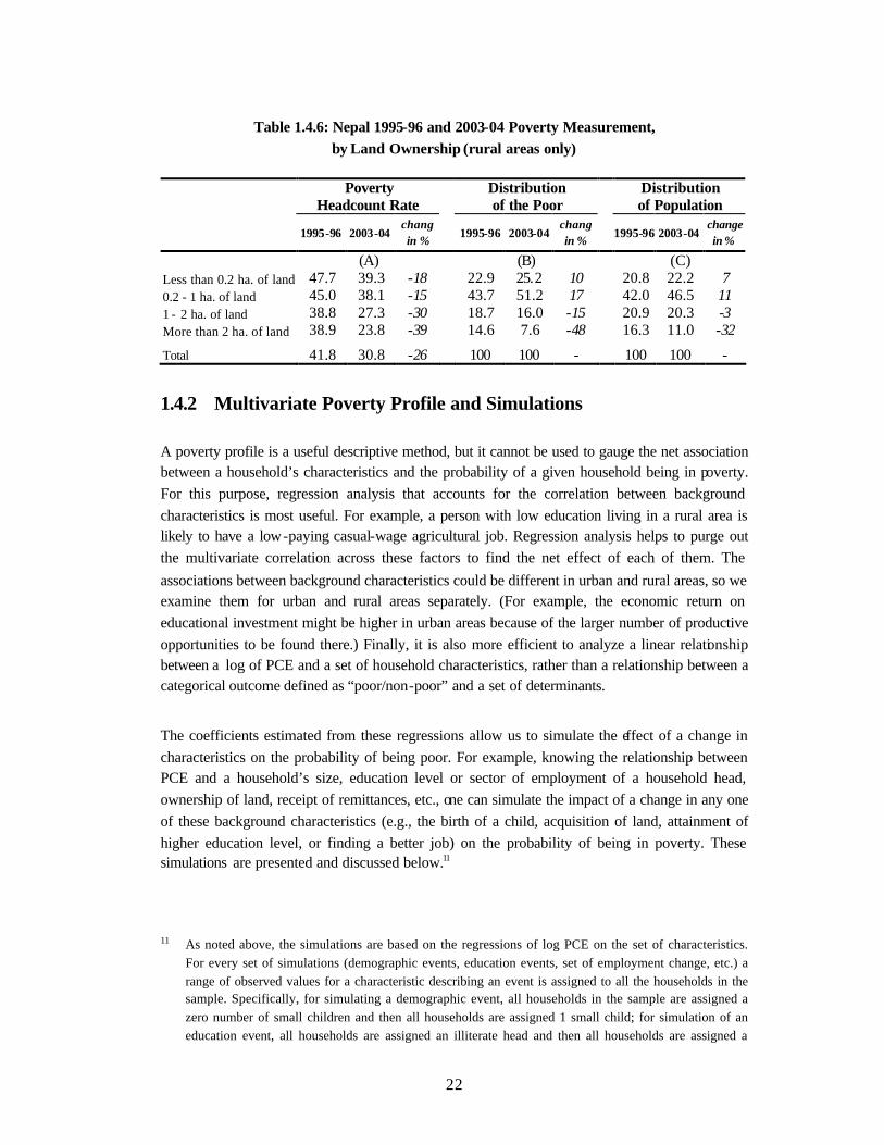
Land ownership
Land ownership reduces the probability of being poor in rural areas, a pattern constant across years. Incidence of poverty among households who own 0.2 ha. or less of land (a quarter of all rural households) is almost 40 percent and is roughly similar to that of households who own 0.2 to 1 ha. (a half of all rural households). Poverty headcount rate had declined more for households with larger landholdings, as compared to the ones with the smaller ones. In addition, the proportion of households with smaller landholdings had increased over time, while the proportion of households with large (2 or more hectares of land) has declined substantially (from 16 to 11 percent of all rural households).
22
Table 1.4.6: Nepal 1995-96 and 2003-04 Poverty Measurement, by Land Ownership (rural areas only)
Poverty Headcount Rate
Distribution of the Poor
Distribution of Population
1995-96 2003-04 chang in %
1995-96 2003-04 chang in %
1995-96 2003-04 change in %
(A) (B) (C) Less than 0.2 ha. of land 47.7 39.3 -18 22.9 25.2 10 20.8 22.2 7 0.2 - 1 ha. of land 45.0 38.1 -15 43.7 51.2 17 42.0 46.5 11 1 - 2 ha. of land 38.8 27.3 -30 18.7 16.0 -15 20.9 20.3 -3 More than 2 ha. of land 38.9 23.8 -39 14.6 7.6 -48 16.3 11.0 -32
Total 41.8 30.8 -26 100 100 - 100 100 -
1.4.2 Multivariate Poverty Profile and Simulations
A poverty profile is a useful descriptive method, but it cannot be used to gauge the net association between a household’s characteristics and the probability of a given household being in poverty. For this purpose, regression analysis that accounts for the correlation between background characteristics is most useful. For example, a person with low education living in a rural area is likely to have a low-paying casual-wage agricultural job. Regression analysis helps to purge out the multivariate correlation across these factors to find the net effect of each of them. The associations between background characteristics could be different in urban and rural areas, so we examine them for urban and rural areas separately. (For example, the economic return on educational investment might be higher in urban areas because of the larger number of productive opportunities to be found there.) Finally, it is also more efficient to analyze a linear relationship between a log of PCE and a set of household characteristics, rather than a relationship between a categorical outcome defined as “poor/non-poor” and a set of determinants.
The coefficients estimated from these regressions allow us to simulate the effect of a change in characteristics on the probability of being poor. For example, knowing the relationship between PCE and a household’s size, education level or sector of employment of a household head, ownership of land, receipt of remittances, etc., one can simulate the impact of a change in any one of these background characteristics (e.g., the birth of a child, acquisition of land, attainment of higher education level, or finding a better job) on the probability of being in poverty. These simulations are presented and discussed below.11
11 As noted above, the simulations are based on the regressions of log PCE on the set of characteristics.
For every set of simulations (demographic events, education events, set of employment change, etc.) a range of observed values for a characteristic describing an event is assigned to all the households in the sample. Specifically, for simulating a demographic event, all households in the sample are assigned a zero number of small children and then all households are assigned 1 small child; for simulation of an education event, all households are assigned an illiterate head and then all households are assigned a
23
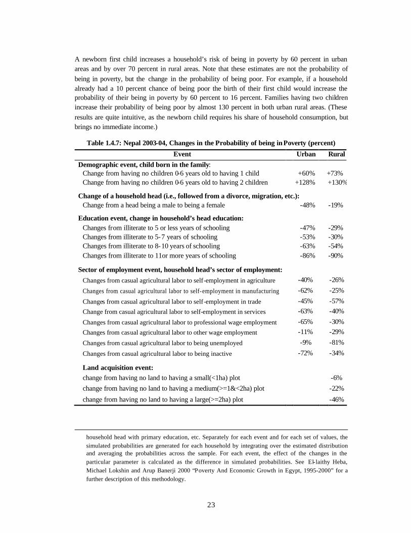
A newborn first child increases a household’s risk of being in poverty by 60 percent in urban areas and by over 70 percent in rural areas. Note that these estimates are not the probability of being in poverty, but the change in the probability of being poor. For example, if a household already had a 10 percent chance of being poor the birth of their first child would increase the probability of their being in poverty by 60 percent to 16 percent. Families having two children increase their probability of being poor by almost 130 percent in both urban rural areas. (These results are quite intuitive, as the newborn child requires his share of household consumption, but brings no immediate income.)
Table 1.4.7: Nepal 2003-04, Changes in the Probability of being in Poverty (percent)
Event Urban Rural Demographic event, child born in the family:
Change from having no children 0-6 years old to having 1 child +60% +73% Change from having no children 0-6 years old to having 2 children +128% +130%
Change of a household head (i.e., followed from a divorce, migration, etc.): Change from a head being a male to being a female -48% -19%
Education event, change in household’s head education: Changes from illiterate to 5 or less years of schooling -47% -29% Changes from illiterate to 5-7 years of schooling -53% -30% Changes from illiterate to 8-10 years of schooling -63% -54% Changes from illiterate to 11or more years of schooling -86% -90%
Sector of employment event, household head’s sector of employment: Changes from casual agricultural labor to self-employment in agriculture -40% -26%
Changes from casual agricultural labor to self-employment in manufacturing -62% -25%
Changes from casual agricultural labor to self-employment in trade -45% -57% Change from casual agricultural labor to self-employment in services -63% -40%
Changes from casual agricultural labor to professional wage employment -65% -30% Changes from casual agricultural labor to other wage employment -11% -29%
Changes from casual agricultural labor to being unemployed -9% -81%
Changes from casual agricultural labor to being inactive -72% -34%
Land acquisition event: change from having no land to having a small(<1ha) plot -6% change from having no land to having a medium(>=1&<2ha) plot -22%
change from having no land to having a large(>=2ha) plot -46%
household head with primary education, etc. Separately for each event and for each set of values, the simulated probabilities are generated for each household by integrating over the estimated distribution and averaging the probabilities across the sample. For each event, the effect of the changes in the particular parameter is calculated as the difference in simulated probabilities. See El-laithy Heba, Michael Lokshin and Arup Banerji 2000 “Poverty And Economic Growth in Egypt, 1995-2000” for a further description of this methodology.
24
Note : T hese estimates show the change in probability of being poor following an event, and not the probability of being in poverty for a household with certain characteristics.
If a household’s head changes from being a male to being a female (for example, by a husband
departing to work elsewhere) the probability of being in poverty is reduced by 48 percent in urban
areas and by 19 percent in rural areas. We reported earlier that female-headed households are more likely to receive remittances, and female headship might pick up some of the positive effect of the receipt of remit tances on consumption.
Changing the education level of a household’s head has a substantial impact on the probability of a household being poor. For example, if an illiterate household head attends primary school, the
probability of this household being in poverty declines by 47 percent in urban and by 29 percent in rural areas. Similarly, acquiring additional education further reduces the chances of being in
poverty. Almost all improvements in poverty incidence following improvements in education
levels are higher in urban as compared to rural areas, possibly indicating a higher economic return to skills in urban areas due to the wider opportunities for gainful employment found there.
Changing the sector of employment for a household’s head from casual agricultural laborer to
self-employment or a variety of other jobs reduces the probability of a family being in poverty. Relative to having a household head being an agricultural wage laborer, being self-employed in
agriculture reduces the chances of being in poverty by 26 percent in rural areas. Being self-employed in manufacturing or trade reduces these chances in rural areas by 25 and 57 percent,
respectively, and in urban areas by 62 and 45 percent, respectively. Being unemployed or inactive also reduces the chances of being in poverty. This may seem counterintuitive. However, these two variables proxy for other household characteristics (e.g., higher initial asset holdings and higher
savings) which allow people to stay out of work, but which are not included in the regression.
Land acquisition by a landless household improves a household’s chances of escaping poverty by 6 percent in the case of accruing a plot of less than 1 hectare, and by 22 and 46 percent,
respectively, in the case of acquiring plots of between 1 and 2 hectares and 2 hectares or more.
1.5 Sensitivity and Robustness of Poverty Estimates
Clearly the poverty estimates presented in Sections 1.2 and 1.4 depend critically on the comparability of surveys on which poverty numbers are based, on the way the poverty line was defined and updated, and also on the choice of welfare measure. In this section we check the
robustness of poverty trends with respect to several measures. First, we examine cumulative distribution functions for real PCE in 1995-96 and 2003-04 to infer whether the choice of poverty
line affects the estimates of trend in headcount poverty. Second, we examine how the fact that the
25
8 Primary Sampling Units (PSUs) that were selected for the cross-sectional sample of NLSS-II, but could not be enumerated, might have affected estimates of poverty incidence. Finally, we
explore alternative approaches to updating and defining poverty lines.
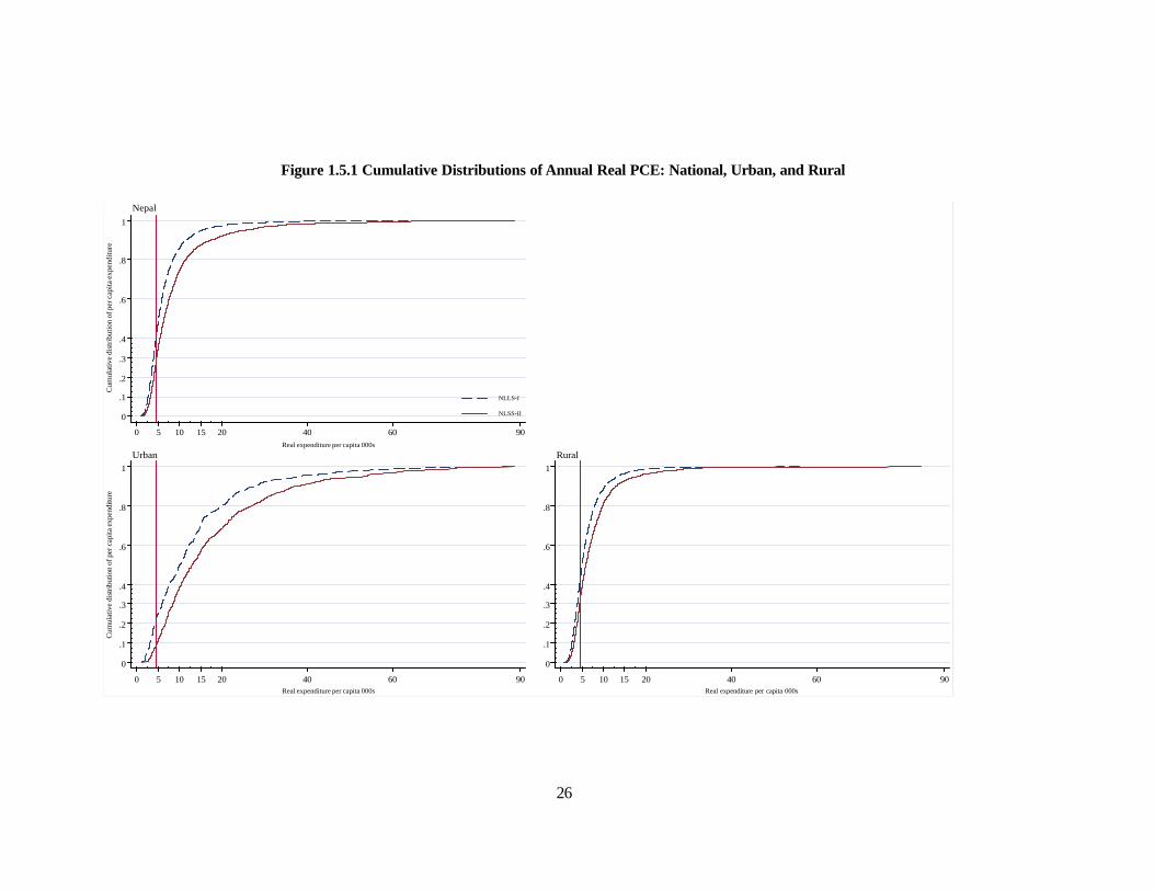
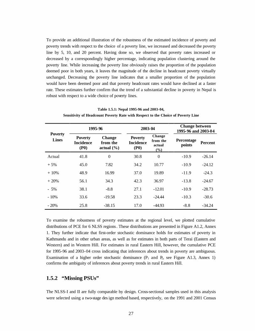
1.5.1 Poverty Incidence Curves
A standard methodology for checking the robustness of poverty estimates is to examine cumulative distributions of real PCE. As mentioned earlier, we use implied poverty line deflators
to express the NLSS-I and NLSS-II consumption aggregates in 1995-96 “average Nepal” prices. Plotted cumulative distributions for PCE at the national, urban, and rural levels (Figure 1.5.1) show that trends in poverty between 1995-96 and 2003-04 are robust in the choice of the poverty line over the range of virtually all other possible poverty lines. This is true for both the urban and
rural sectors – the cumulative distributions for real PCE in 2003-04 are everywhere below and to
the right of the cumulative distributions for 1995-96, indicating first-order stochastic dominance.
26
0
.1
.2
.3
.4
.6
.8
1
Cum
ulat
ive
dist
ribu
tion
of p
er c
apita
exp
endi
ture
0 20 40 60 905 10 15Real expenditure per capita 000s
NLLS-I
NLSS-II
Nepal
0
.1
.2
.3
.4
.6
.8
1
Cum
ulat
ive
dist
ribut
ion
of p
er c
apita
exp
endi
ture
0 20 40 60 905 10 15Real expenditure per capita 000s
Urban
0
.1
.2
.3
.4
.6
.8
1
0 20 40 60 905 10 15Real expenditure per capita 000s
Rural
Figure 1.5.1 Cumulative Distributions of Annual Real PCE: National, Urban, and Rural
27
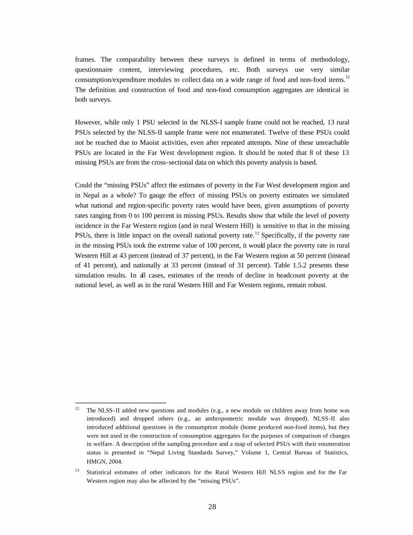
To provide an additional illustration of the robustness of the estimated incidence of poverty and poverty trends with respect to the choice of a poverty line, we increased and decreased the poverty line by 5, 10, and 20 percent. Having done so, we observed that poverty rates increased or decreased by a correspondingly higher percentage, indicating population clustering around the poverty line. While increasing the poverty line obviously raises the proportion of the population deemed poor in both years, it leaves the magnitude of the decline in headcount poverty virtually unchanged. Decreasing the poverty line indicates that a smaller proportion of the population would have been deemed poor and that poverty headcount rates would have declined at a faster rate. These estimates further confirm that the trend of a substantial decline in poverty in Nepal is robust with respect to a wide choice of poverty lines.
Table 1.5.1: Nepal 1995-96 and 2003-04,
Sensitivity of Headcount Poverty Rate with Respect to the Choice of Poverty Line
1995-96 2003-04 Change between 1995-96 and 2003-04
Poverty Lines Poverty
Incidence (P0)
Change from the
actual (%)
Poverty Incidence
(P0)
Change from the actual
(%)
Percentage points Percent
Actual 41.8 0 30.8 0 -10.9 -26.14
+ 5% 45.0 7.82 34.2 10.77 -10.9 -24.12
+ 10% 48.9 16.99 37.0 19.89 -11.9 -24.3
+ 20% 56.1 34.3 42.3 36.97 -13.8 -24.67
- 5% 38.1 -8.8 27.1 -12.01 -10.9 -28.73
- 10% 33.6 -19.58 23.3 -24.44 -10.3 -30.6
- 20% 25.8 -38.15 17.0 -44.93 -8.8 -34.24
To examine the robustness of poverty estimates at the regional level, we plotted cumulative distributions of PCE for 6 NLSS regions . These distributions are presented in Figure A1.2, Annex 1. They further indicate that first-order stochastic dominance holds for estimates of poverty in Kathmandu and in other urban areas, as well as for estimates in both parts of Terai (Eastern and Western) and in Western Hill. For estimates in rural Eastern Hill, however, the cumulative PCE for 1995-96 and 2003-04 cross indicating that inferences about trends in poverty are ambiguous. Examination of a higher order stochastic dominance (P1 and P2, see Figure A1.3, Annex 1) confirms the ambiguity of inferences about poverty trends in rural Eastern Hill.
1.5.2 “Missing PSUs”
The NLSS-I and II are fully comparable by design. Cross-sectional samples used in this analysis were selected using a two-stage des ign method based, respectively, on the 1991 and 2001 Census
28
frames. The comparability between these surveys is defined in terms of methodology, questionnaire content, interviewing procedures, etc. Both surveys use very similar consumption/expenditure modules to collect data on a wide range of food and non-food items.12 The definition and construction of food and non-food consumption aggregates are identical in both surveys.
However, while only 1 PSU selected in the NLSS-I sample frame could not be reached, 13 rural PSUs selected by the NLSS-II sample frame were not enumerated. Twelve of these PSUs could not be reached due to Maoist activities, even after repeated attempts. Nine of these unreachable PSUs are located in the Far West development region. It shou ld be noted that 8 of these 13 missing PSUs are from the cross-sectional data on which this poverty analysis is based.
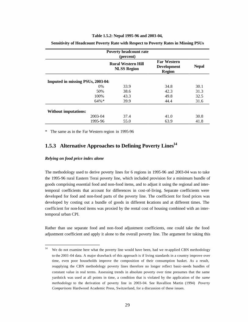
Could the “missing PSUs” affect the estimates of poverty in the Far West development region and in Nepal as a whole? To gauge the effect of missing PSUs on poverty estimates we simulated what national and region-specific poverty rates would have been, given assumptions of poverty rates ranging from 0 to 100 percent in missing PSUs. Results show that while the level of poverty incidence in the Far Western region (and in rural Western Hill) is sensitive to that in the missing PSUs, there is little impact on the overall national poverty rate.13 Specifically, if the poverty rate in the missing PSUs took the extreme value of 100 percent, it would place the poverty rate in rural Western Hill at 43 percent (instead of 37 percent), in the Far Western region at 50 percent (instead of 41 percent), and nationally at 33 percent (instead of 31 percent). Table 1.5.2 presents these simulation results. In all cases, estimates of the trends of decline in headcount poverty at the national level, as well as in the rural Western Hill and Far Western regions, remain robust.
12 The NLSS-II added new questions and modules (e.g., a new module on children away from home was
introduced) and dropped others (e.g., an anthropometric module was dropped). NLSS-II also introduced additional questions in the consumption module (home produced non-food items), but they were not used in the construction of consumption aggregates for the purposes of comparison of changes in welfare. A description of the sampling procedure and a map of selected PSUs with their enumeration status is presented in “Nepal Living Standards Survey,” Volume 1, Central Bureau of Statistics, HMGN, 2004.
13 Statistical estimates of other indicators for the Rural Western Hill NLSS region and for the Far Western region may also be affected by the “missing PSUs”.
29
Table 1.5.2: Nepal 1995-96 and 2003-04,
Sensitivity of Headcount Poverty Rate with Respect to Poverty Rates in Missing PSUs
Poverty headcount rate (percent)
Rural Western Hill NLSS Region
Far Western Development
Region Nepal
Imputed in missing PSUs, 2003-04:
0% 33.9 34.8 30.1 50% 38.6 42.3 31.3
100% 43.3 49.8 32.5 64%* 39.9 44.4 31.6
Without imputations:
2003-04 37.4 41.0 30.8 1995-96 55.0 63.9 41.8
* The same as in the Far Western region in 1995-96
1.5.3 Alternative Approaches to Defining Poverty Lines14
Relying on food price index alone
The methodology used to derive poverty lines for 6 regions in 1995-96 and 2003-04 was to take the 1995-96 rural Eastern Terai poverty line, which included provision for a minimum bundle of goods comprising essential food and non-food items, and to adjust it using the regional and inter-temporal coefficients that account for differences in cost-of-living. Separate coefficients were developed for food and non-food parts of the poverty line. The coefficient for food prices was developed by costing out a bundle of goods in different locations and at different times. The coefficient for non-food items was proxied by the rental cost of housing combined with an inter-temporal urban CPI.
Rather than use separate food and non-food adjustment coefficients, one could take the food adjustment coefficient and apply it alone to the overall poverty line. The argument for taking this
14 We do not examine here what the poverty line would have been, had we re-applied CBN methodology
to the 2003 -04 data. A major drawback of this approach is if living standards in a country improve over time, even poor households improve the composition of their consumption basket. As a result, reapplying the CBN methodology poverty lines therefore no longer reflect basic-needs bundles of
constant value in real terms. Assessing trends in absolute poverty over time presumes that the same yardstick was used at all points in time, a condition that is violated by the application of the same methodology to the derivation of poverty line in 2003-04. See Ravallion Martin (1994) Poverty Comparisons Hardwood Academic Press, Switzerland, for a discussion of these issues.
30
approach is that the food coefficient is calculated on the basis of an actual bundle consumed by the poor, while the non-food coefficient relies on proxies. In fact Deaton (see Deaton 2004) took this approach and used only the differences in prices of food items (plus fuel and wood) to adjust for differences in cost of living across Indian states and over time. The drawback, of course, is that the prices of only a sub-set of the total consumption bundle (which is also declining over time as the proportion of food in the consumption bundle declines) are used to adjust the poverty line. Nevertheless, as a check for sensitivity of poverty estimates, we performed calculations based solely on the food price index. 15 16
Table 1.5.3 shows that estimates in 1995-96 and in 2003-04 obtained by this method are very close to the preferred estimates of poverty incidence. Regional rankings stay the same, while estimates for 1995-96 and 2003-04 are on the high and low sides, respectively, of the preferred estimates for those years. Consequently, the estimates of decline in poverty rate are even higher than if one utilizes both food and non-food adjustment coefficients for the respective parts of the poverty line.
Table 1.5.3: Nepal 1995-96 and 2003-04, Poverty Headcount Rate across Regions
(based on food price adjustment indices alone)
1995-96 2003-04
Change (percentage
points) Change (percent)
Kathmandu 1.9 2.2 0.4 20
Other Urban 29.4 11.3 -18.1 -61
R. Western Hill 58.5 33.0 -25.5 -44
R. Eastern Hill 37.1 42.9 5.8 16
R. Western Terai 50.5 26.1 -24.4 -48
R. Eastern Terai 37.2 30.3 -6.9 -19
Nepal 43.4 29.5 -13.9 -32
15 Another possibility would be to use the Rasta Bank CPI for the purpose of inter-temporal adjustment.
Recall, however, that only urban CPI is available and, in case of food items, it is very close to the estimated survey -based coefficient. Because of this, we do not examine the sensitivity of poverty estimates with respect to the official CPI.
16 Food price adjustment coefficients alone are applied to adjust for the regional and inter -temporal differences in prices. Consequently, poverty estimates for 1995-96 are also different from the preferred poverty estimates.
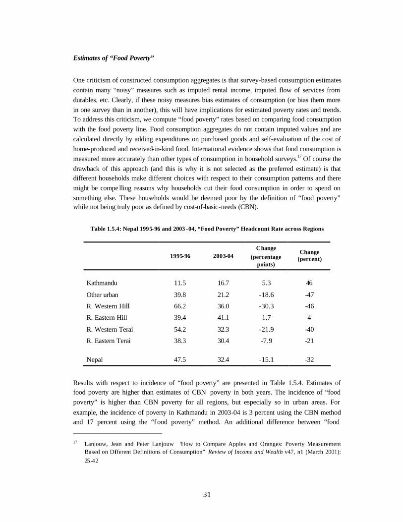
31
Estimates of “Food Poverty”
One criticism of constructed consumption aggregates is that survey-based consumption estimates contain many “noisy” measures such as imputed rental income, imputed flow of services from durables, etc. Clearly, if these noisy measures bias estimates of consumption (or bias them more in one survey than in another), this will have implications for estimated poverty rates and trends. To address this criticism, we compute “food poverty” rates based on comparing food consumption with the food poverty line. Food consumption aggregates do not contain imputed values and are calculated directly by adding expenditures on purchased goods and self-evaluation of the cost of home-produced and received-in-kind food. International evidence shows that food consumption is measured more accurately than other types of consumption in household surveys.17 Of course the drawback of this approach (and this is why it is not selected as the preferred estimate) is that different households make different choices with respect to their consumption patterns and there might be compe lling reasons why households cut their food consumption in order to spend on something else. These households would be deemed poor by the definition of “food poverty” while not being truly poor as defined by cost-of-basic-needs (CBN).
Table 1.5.4: Nepal 1995-96 and 2003 -04, “Food Poverty” Headcount Rate across Regions
1995-96 2003-04 Change
(percentage points)
Change (percent)
Kathmandu 11.5 16.7 5.3 46
Other urban 39.8 21.2 -18.6 -47
R. Western Hill 66.2 36.0 -30.3 -46
R. Eastern Hill 39.4 41.1 1.7 4
R. Western Terai 54.2 32.3 -21.9 -40
R. Eastern Terai 38.3 30.4 -7.9 -21
Nepal 47.5 32.4 -15.1 -32
Results with respect to incidence of “food poverty” are presented in Table 1.5.4. Estimates of food poverty are higher than estimates of CBN poverty in both years. The incidence of “food poverty” is higher than CBN poverty for all regions, but especially so in urban areas. For example, the incidence of poverty in Kathmandu in 2003-04 is 3 percent using the CBN method and 17 percent using the “food poverty” method. An additional difference between “food
17 Lanjouw, Jean and Peter Lanjouw “How to Compare Apples and Oranges: Poverty Measurement
Based on Different Definitions of Consumption” Review of Income and Wealth v47, n1 (March 2001): 25-42
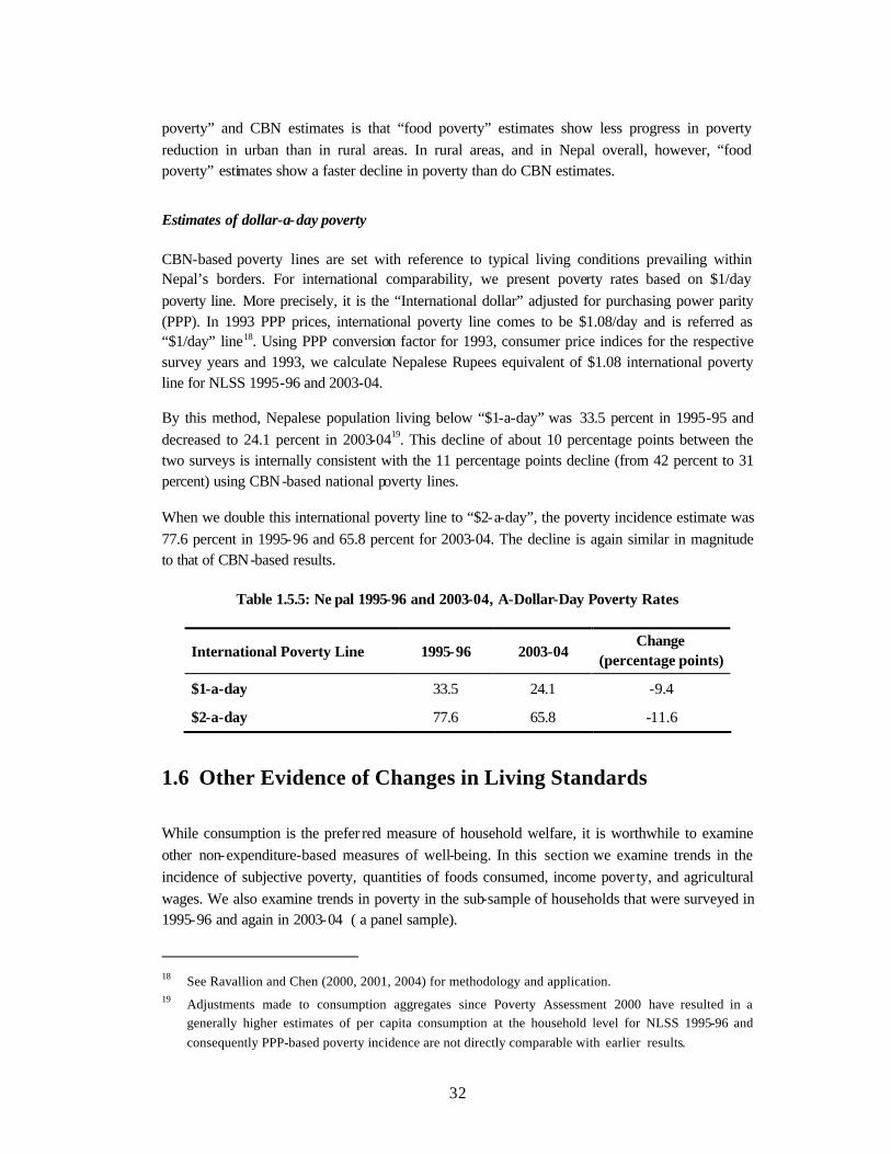
32
poverty” and CBN estimates is that “food poverty” estimates show less progress in poverty reduction in urban than in rural areas. In rural areas, and in Nepal overall, however, “food poverty” estimates show a faster decline in poverty than do CBN estimates.
Estimates of dollar-a-day poverty
CBN-based poverty lines are set with reference to typical living conditions prevailing within Nepal’s borders. For international comparability, we present poverty rates based on $1/day poverty line. More precisely, it is the “International dollar” adjusted for purchasing power parity (PPP). In 1993 PPP prices, international poverty line comes to be $1.08/day and is referred as “$1/day” line18. Using PPP conversion factor for 1993, consumer price indices for the respective survey years and 1993, we calculate Nepalese Rupees equivalent of $1.08 international poverty line for NLSS 1995-96 and 2003-04.
By this method, Nepalese population living below “$1-a-day” was 33.5 percent in 1995-95 and decreased to 24.1 percent in 2003-0419. This decline of about 10 percentage points between the two surveys is internally consistent with the 11 percentage points decline (from 42 percent to 31 percent) using CBN-based national poverty lines.
When we double this international poverty line to “$2-a-day”, the poverty incidence estimate was 77.6 percent in 1995-96 and 65.8 percent for 2003-04. The decline is again similar in magnitude to that of CBN-based results.
Table 1.5.5: Ne pal 1995-96 and 2003-04, A-Dollar-Day Poverty Rates
International Poverty Line 1995-96 2003-04 Change
(percentage points)
$1-a-day 33.5 24.1 -9.4
$2-a-day 77.6 65.8 -11.6
1.6 Other Evidence of Changes in Living Standards
While consumption is the prefer red measure of household welfare, it is worthwhile to examine other non-expenditure-based measures of well-being. In this section we examine trends in the incidence of subjective poverty, quantities of foods consumed, income pover ty, and agricultural wages. We also examine trends in poverty in the sub-sample of households that were surveyed in 1995-96 and again in 2003-04 ( a panel sample).
18 See Ravallion and Chen (2000, 2001, 2004) for methodology and application. 19 Adjustments made to consumption aggregates since Poverty Assessment 2000 have resulted in a
generally higher estimates of per capita consumption at the household level for NLSS 1995-96 and consequently PPP-based poverty incidence are not directly comparable with earlier results.
33
1.6.1 Subjective Poverty Line
Another way to estimate poverty is to analyze self-reported information about the adequacy of consumption on the basis of answers to NLSS-collected minimum income questions (MIQs). Both the MIQ results and the constructed poverty rate can be used to judge the progress in living standards. NLSS-I and NLSS-II collected information according to the schedule presented in Table 1.6.1.
Results reveal an improvement in perception of all aspects of standards of living. While almost 50 percent of households responded that food consumption was inadequate in 1995-96, the number reporting this in 2003-04 decreased to 30 percent. With regard to housing, the reduction is even larger. There are also improvements in the perception of adequacy of health care and children’s schooling. Respondents were most dissatisfied with their family’s income, although this proportion is also decreasing.20
Table 1.6.1: Nepal 1995-96 and 2003-04, Self-reported Assessment of Consumption Adequacy
“It was less than adequate for your family
needs?”* “I would like to ask your opinion of your family’s standard of living”
1995-96 2003-04
Concerning your family’s food consumption over the past one month, which of the following is true ?
49 30
Concerning your family’s housing consumption over the past one month, which of the following is true ?
64 40
Concerning your family’s clothing consumption over the past one month, which of the following is true ?
57 36
Concerning the health care your family’s gets, which of the following is true ?** 59 28
Concerning your children’s schooling , which of the following is true ?** 48 23
Concerning your family’s total income over the past one month, which of the following is true ?
71 66
Do you consider that you, or your family eats too little to live a health and active life ? (percentage of respondents answering “yes”)
90 87
* Response options offered to respondents were: “It was less than adequate for your family needs”; “It was just adequate for your family needs”; “It was more than adequate for your family needs”; and, “Not applicable”.
** Since “not applicable” was a possible answer, “less than adequate” responses to this question were naturally fewer than the others.
20 We are not sure how to interpret the response in the last row of Table 1.6.1 which seems to contradict
the response in the first row of the same table.
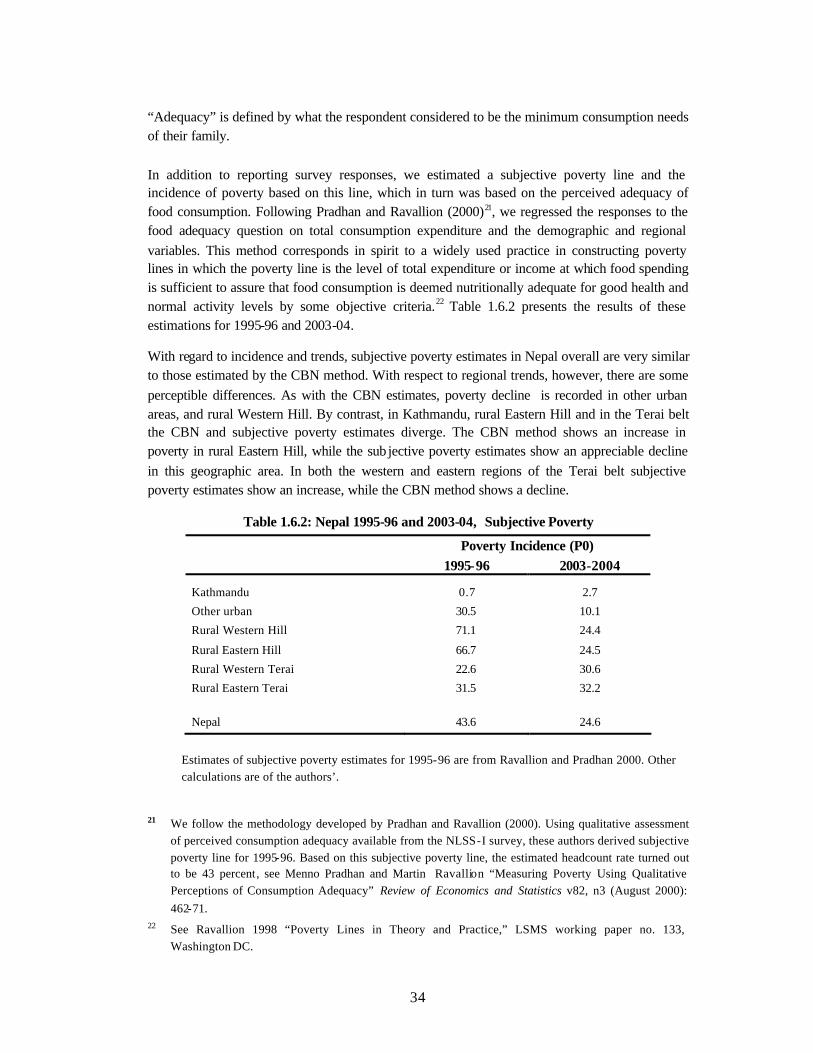
34
“Adequacy” is defined by what the respondent considered to be the minimum consumption needs of their family.
In addition to reporting survey responses, we estimated a subjective poverty line and the incidence of poverty based on this line, which in turn was based on the perceived adequacy of food consumption. Following Pradhan and Ravallion (2000)21, we regressed the responses to the food adequacy question on total consumption expenditure and the demographic and regional variables. This method corresponds in spirit to a widely used practice in constructing poverty lines in which the poverty line is the level of total expenditure or income at which food spending is sufficient to assure that food consumption is deemed nutritionally adequate for good health and normal activity levels by some objective criteria.22 Table 1.6.2 presents the results of these estimations for 1995-96 and 2003-04.
With regard to incidence and trends, subjective poverty estimates in Nepal overall are very similar to those estimated by the CBN method. With respect to regional trends, however, there are some perceptible differences. As with the CBN estimates, poverty decline is recorded in other urban areas, and rural Western Hill. By contrast, in Kathmandu, rural Eastern Hill and in the Terai belt the CBN and subjective poverty estimates diverge. The CBN method shows an increase in poverty in rural Eastern Hill, while the sub jective poverty estimates show an appreciable decline in this geographic area. In both the western and eastern regions of the Terai belt subjective poverty estimates show an increase, while the CBN method shows a decline.
Table 1.6.2: Nepal 1995-96 and 2003-04, Subjective Poverty
Estimates of subjective poverty estimates for 1995-96 are from Ravallion and Pradhan 2000. Other calculations are of the authors’.
21 We follow the methodology developed by Pradhan and Ravallion (2000). Using qualitative assessment
of perceived consumption adequacy available from the NLSS-I survey, these authors derived subjective poverty line for 1995-96. Based on this subjective poverty line, the estimated headcount rate turned out to be 43 percent, see Menno Pradhan and Martin Ravallion “Measuring Poverty Using Qualitative Perceptions of Consumption Adequacy” Review of Economics and Statistics v82, n3 (August 2000): 462-71.
22 See Ravallion 1998 “Poverty Lines in Theory and Practice,” LSMS working paper no. 133, Washington DC.
Poverty Incidence (P0) 1995-96 2003-2004
Kathmandu 0.7 2.7
Other urban 30.5 10.1
Rural Western Hill 71.1 24.4
Rural Eastern Hill 66.7 24.5
Rural Western Terai 22.6 30.6
Rural Eastern Terai 31.5 32.2 Nepal 43.6 24.6
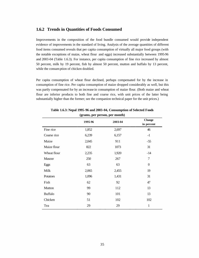
35
1.6.2 Trends in Quantities of Foods Consumed
Improvements in the composition of the food bundle consumed would provide independent evidence of improvements in the standard of living. Analysis of the average quantities of different food items consumed reveals that per capita consumption of virtually all major food groups (with the notable exceptions of maize, wheat flour and eggs) increased substantially between 1995-96 and 2003-04 (Table 1.6.3). For instance, per capita consumption of fine rice increased by almost 50 percent, milk by 19 percent, fish by almost 50 percent, mutton and buffalo by 13 percent, while the consumption of chicken doubled.
Per capita consumption of wheat flour declined, perhaps compensated for by the increase in consumption of fine rice. Per capita consumption of maize dropped considerably as well, but this was partly compensated for by an increase in consumption of maize flour. (Both maize and wheat flour are inferior products to both fine and coarse rice, with unit prices of the latter being substantially higher than the former; see the companion technical paper for the unit prices.)
Table 1.6.3: Nepal 1995-96 and 2003-04, Consumption of Selected Foods (grams, per person, per month)
1995-96 2003-04 Change
in percent
Fine rice 1,852 2,697 46
Coarse rice 6,239 6,157 -1
Maize 2,045 911 -55
Maize flour 822 1073 31
Wheat flour 2,235 1,920 -14
Masoor 250 267 7
Eggs 63 63 0
Milk 2,065 2,455 19
Potatoes 1,096 1,431 31
Fish 62 92 47
Mutton 99 112 13
Buffalo 90 101 13
Chicken 51 102 102
Tea 29 29 1
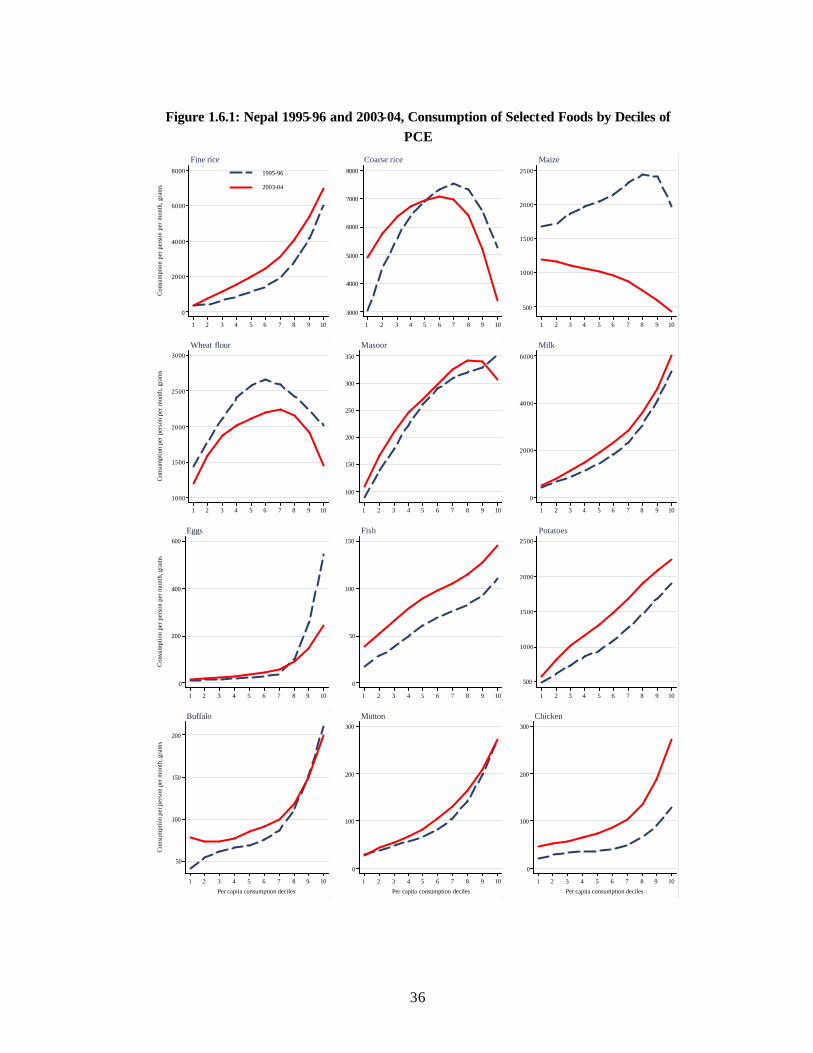
36
Figure 1.6.1: Nepal 1995-96 and 2003-04, Consumption of Selected Foods by Deciles of PCE
0
2000
4000
6000
8000
Con
sum
ptio
n pe
r pe
rson
per
mon
th, g
ram
s
1 2 3 4 5 6 7 8 9 10
1995-96
2003-04
Fine rice
3000
4000
5000
6000
7000
8000
1 2 3 4 5 6 7 8 9 10
Coarse rice
500
1000
1500
2000
2500
1 2 3 4 5 6 7 8 9 10
Maize
1000
1500
2000
2500
3000
Con
sum
ptio
n pe
r pe
rson
per
mon
th, g
ram
s
1 2 3 4 5 6 7 8 9 10
Wheat flour
100
150
200
250
300
350
1 2 3 4 5 6 7 8 9 10
Masoor
0
2000
4000
6000
1 2 3 4 5 6 7 8 9 10
Milk
0
200
400
600
Con
sum
ptio
n pe
r per
son
per m
onth
, gra
ms
1 2 3 4 5 6 7 8 9 10
Eggs
0
50
100
150
1 2 3 4 5 6 7 8 9 10
Fish
500
1000
1500
2000
2500
1 2 3 4 5 6 7 8 9 10
Potatoes
50
100
150
200
Con
sum
ptio
n pe
r per
son
per m
onth
, gra
ms
1 2 3 4 5 6 7 8 9 10
Per capita consumption deciles
Buffalo
0
100
200
300
1 2 3 4 5 6 7 8 9 10
Per capita consumption deciles
Mutton
0
100
200
300
1 2 3 4 5 6 7 8 9 10
Per capita consumption deciles
Chicken
37
Figure 1.6.1 depicts per capita consumption of selected foods by deciles of PCE distribution in 1995-96 and 2003-04. It shows that the trends reported above are not confined to high-income groups. In fact, percentage increases in the consumption of fine rice, as well as in all groups of vegetable and animal proteins and fats, were higher among low-income households than among high-income households. (See Annex 1, Table A1.2 for the actual amounts of foods consumed by low -income households.)
1.6.3 Evidence from a Panel Sample
The poverty estimates discussed above are based on NLSS-I and a cross-sectional component of NLSS-II. These two samples are representative of the population of Nepal in 1995-96 and 2003-04, respectively. In addition, NLSS-II attempted to collect data from about 1,200 NLSS-I-surveyed households. Nine hundred and sixty-two of them were located, comprising a panel component of NLSS-I and NLSS-II.
We examined this panel component to gain further insight into the dynamics of poverty between 1995-96 and 2003-04. Table 1.6.4 presents a transition matrix with respect to poverty status for the households in the panel sample.
Table 1.6.4 Nepal 1994-95 and 2003-04, Transition Matrix in and out of Poverty (Panel sample)
2003-04
Non-poor Poor All Non-poor Poor All Non-poor Poor All
All Urban Rural
Non-poor 47.6 13.6 61.2 60.4 7.4 67.9 46.8 14.1 60.9
Poor 20.4 18.5 38.8 19.7 12.4 32.2 20.7 18.5 39.1
1995
-96
Total 68.0 32.0 100.0 80.1 19.9 100 67.5 32.5 100
The CBN poverty rate for the panel sample in 1995-96 was estimated at 38.8 percent, while for 2003-04 it was estimated at 32.0 percent. These estimates are quite close to the estimates obtained from the main cross-sectional samples, confirming the trend of substantial poverty decline in Nepal. (Note that the 2003-04 panel sample doesn’t represent the 2003-04 population of Nepal, while the 2003-04 cross-sectional sample does. Therefore, 2003-04 poverty estimates obtained from the cross-sectional sample are the preferred ones.) In urban areas, the poverty rate in 1995-96 was 32.2 percent. It dropped to 19.9 percent in 2003-04. These estimates are considerably higher than the 21.55 and 9.55 percent poverty rates estimated from the cross-sectional NLSS-I
38
and II. This most likely indicates that the panel failed to follow the most-wealthy households in urban areas. This is a standard problem in panels, especially when the time between the surveys is as long as 8 years, as was the case here.
In the rural panel, the poverty rate in 1995-96 was 39.1 percent. It dropped to 32.5 percent in 2003-04. These estimates are close to the estimates obtained from the cross-section sample.
Estimates from the panel in both urban and rural areas confirm the trends of a substantial drop in poverty. While these trends show that many households moved out of poverty, they also attest to the downward variability in expenditures and a household’s non-negligible chances of falling into poverty.
1.6.4 Trends in Agricultural Wages
International evidence suggests that real agricultural wages tend to be highly correlated with poverty headcount ratios, and areas with low agricultural wages tend to have higher poverty headcounts.23 In addition, Deaton and Dreze (2002) suggest interpreting real wage as a poverty indicator in its own right. If the labor market is competitive, the real wage measures the “reservation wage,” i.e., the lowest wage at which laborers are prepared to work. This could be interpreted as an indication of the degree of deprivation (the more desperate people are, the lower the reservation wage), independent of the statistical association between real wages and the headcount ratio.
Wages earned by agricultural laborers represent an important indicator of welfare in rural Nepal as well. Table 1.6.5 presents 3 types of agricultural wage statistics. First, it presents nominal daily wages in 1995-96 and 2003-04; second, it presents real daily wages obtained by applying implicit poverty deflators to real wages; and third, it presents daily wages expressed as kilograms of rice. By all three measures daily wages of agricultural laborers increased. In Eastern Terai, wages increased the least of all regions, possibly reflecting the relative abundance of agricultural labor in that region. 24. Surprisingly, wages of agricultural laborers in Eastern Hill increased quite fast, but without the commensurate reduction in the incidence of poverty in the region.
23 Deaton and Dreze (2002) present evidence that real agricultural wages are highly (0.79) correlated with
rural headcount ratios across Indian states. See Deaton A. and Dreze J. “Poverty and Inequality in India: A re-examination”. Economic and Political Weekly. September 7, 2002.
24 In Nepal, agricultural wage labor is most prevalent in the Terai belt, especially in rural Eastern Terai. In fact, over 65 percent of those who are engaged in agricultural labor as their main occupation reside in Eastern Terai alone, see “Nepal Living Standards Survey 2003/04 Statistical Report”, Volume 2, Central Bureau of Statistics, National Planning Commission Secretariat, HMGN, December 2004.
39
Table 1.6.5: Nepal 1995-96 and 2003-04 Agricultural Wages by Geographic Region (Rural Areas)
Nominal
Agricultural Daily Wage (NRS)
Real Agricultural Daily Wage (NRS)
Real Agricultural Daily Wage (kg of rice)
1995-96 2003-04 chang in %
1995-96 2003-04 chang in %
1995-96 2003-04 change in %
(A) (B) (C)
Western Hill 49 90 84 49 54 10 3 4 33
Eastern Hill 37 86 132 37 54 46 2 4 100
Western Terai 50 89 78 50 63 26 4 6 50
Eastern Terai 43 61 42 43 54 26 3 4 33
1.6.5 Trends in Income Poverty
Both NLSS-I and II contain extensive modu les on total earnings from different income sources – wage employment, non-agricultural enterprises, agricultural enterprises, remittances, and other
income. For each individual in the household (aged 10 years and older in NLSS-I, and aged 5 years and older in NLSS-II), information on time worked, sector of employment (occupation and industry), and amount earned from each economic activity is collected. This enabled the construction of comparable per-capita income and consumption measures, which in turn can be
used to estimate the incidence of poverty (Table 1.6.6.)
Estimates of income-based poverty are obtaining by comparing year and region-specific poverty
lines with nominal aggregate per -capita income (instead of aggregate per-capita expenditures as in the CBN method). These estimates are very closely aligned with estimates of poverty based on
consumption expenditures.25 For example, for 1995-96, poverty estimates based on income are about 5 percentage points higher than those based on per capita consumption (47 percent versus
42 percent); for 2003-04 the difference is 4 percentage points (31 percent versus 35 percent). Estimates of poverty decline (11 percentage points in the case of consumption poverty, and 12
percentage points in the case of income poverty) are also quite close.
25 Note that several components (imputed rent from the owner occupied housing and value of home
produced non -crop consumption) enter both measures. However, this fact alone cannot account for these similar patterns. The common components represent only 15(18) percent in income and expenditure respectively. (For the households in the lowest and second lowest PCE quintiles , the common component represents 11(14) and 13(14) percent, respectively). Correlation between income and expenditure for the whole sample is 0.72; excluding the common components from the income and consumption reduces the correlation to 0.58.
40
As with consumption-based poverty estimates, income-based poverty estimates show that rural poverty is considerably higher than urban poverty both in 1995-96 and 2003-04. Regional patterns are also broadly similar. Other urban ar eas and rural Western Hill had a greater -than-average decline in income-based poverty similar to that of consumption-based poverty. Contrary to the trend of increasing consumption-based poverty in rural Eastern Hill, income-based poverty estimates show a decline.
Table 1.6.6: Nepal 1995-96 and 2003-04,
Income-based Poverty Estimates
1995-96 2003-2004
Change (percentage
points)
Change (percent)
Urban 26.2 12.5 -13.7 -52
Rural 48.8 38.8 -10.0 -20 Kathmandu 6.8 4.7 -2.1 -31
Other urban 37.4 16.8 -20.6 -55
Rural Western Hill 62.0 43.6 -18.5 -30
Rural Eastern Hill 54.1 45.7 -8.4 -16
Rural Western Terai 41.8 33.8 -8.0 -19
Rural Eastern Terai 37.4 33.3 -4.1 -11 Nepal 47.2 34.9 -12.4 -26
1.7 Tentative Explanations for the Observed Increase in Per Capita Income and Expenditure and Decline in Poverty
Average real per -capita household expenditures in Nepal grew at the rate of 4.5 percent per year between 1995-96 and 2003-04. This represents a remarkable achievement by international standards. While patterns of growth were not pro-poor per se and inequality has increased, because of the magnitude of this growth incidence of poverty declined by 11 percentage points (or 26 percent over 8 years) which also represents a remarkable achievement. Evidence from elsewhere shows that in addition to consumption and income gains, there also were improvements in human development indicators in Nepal.26 Given Nepal’s ongoing and Maoist insurgency, which deters investments and other economic activities, impedes the delivery of services, and costs human lives, these results represent a surprising picture of resilience of the Nepalese people against the backdrop of failing state institutions. What structural economic changes can explain these achievements ? 26 See “Nepal Living Standards Survey 2003-04”, CBS, HMGN.
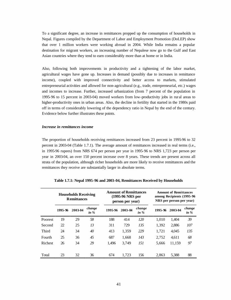
41
To a significant degree, an increase in remittances propped up the consumption of households in Nepal. Figures compiled by the Department of Labor and Employment Promotion (DoLEP) show that over 1 million workers were working abroad in 2004. While India remains a popular destination for migrant workers, an increasing number of Nepalese now go to the Gulf and East Asian countries where they tend to earn considerably more than at home or in India.
Also, following both improvements in productivity and a tightening of the labor market, agricultural wages have gone up. Increases in demand (possibly due to increases in remittance income), coupled with improved connectivity and better access to markets, stimulated entrepreneurial activities and allowed for non-agricultural (e.g., trade, entrepreneurial, etc.) wages and incomes to increase. Further, increased urbanization (from 7 percent of the population in 1995-96 to 15 percent in 2003-04) moved workers from low-productivity jobs in rural areas to higher-productivity ones in urban areas. Also, the decline in fertility that started in the 1980s paid off in terms of considerably lowering of the dependency ratio in Nepal by the end of the century. Evidence below further illustrates these points.
Increase in remittances income
The proportion of households receiving remittances increased from 23 percent in 1995-96 to 32 percent in 2003-04 (Table 1.7.1). The average amount of remittances increased in real terms (i.e., in 1995-96 rupees) from NRS 674 per person per year in 1995-96 to NRS 1,723 per person per year in 2003-04, an over 150 percent increase over 8 years. These trends are present across all strata of the population, although richer households are more likely to receive remittances and the remittances they receive are substantially larger in absolute terms.
Table 1.7.1: Nepal 1995-96 and 2003-04, Remittances Received by Households
Households Receiving Remittances
Amount of Remittances
(1995-96 NRS per person per year)
Amount of Remittances
among Recipients (1995-96 NRS per person per year)
1995-96 2003-04 change in %
1995-96 2003-04 change in %
1995-96 2003-04 change in %
Poorest 19 29 58 188 414 120 1,010 1,404 39 Second 22 25 13 311 729 135 1,392 2,886 107 Third 24 34 40 413 1,359 229 1,721 4,045 135
Fourth 25 36 45 687 1,668 143 2,752 4,611 68 Richest 26 34 29 1,496 3,749 151 5,666 11,159 97 Total 23 32 36 674 1,723 156 2,863 5,388 88
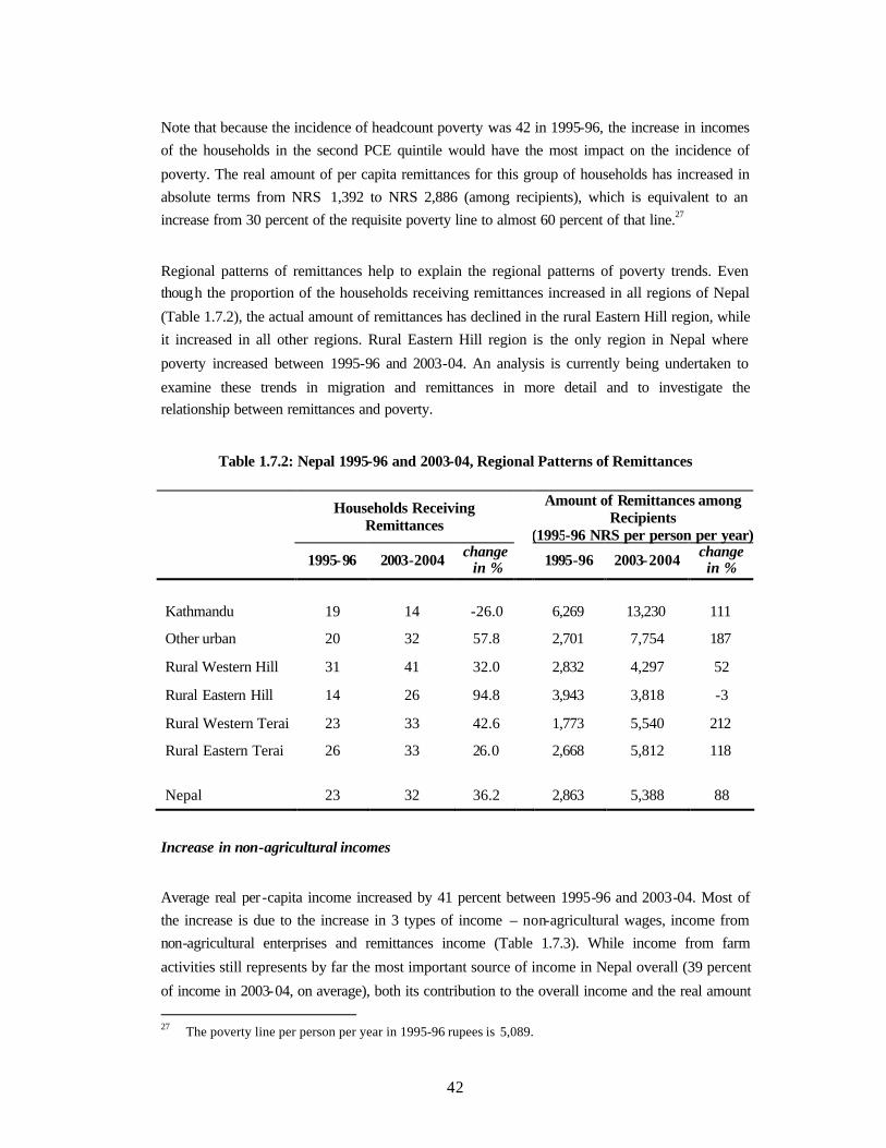
42
Note that because the incidence of headcount poverty was 42 in 1995-96, the increase in incomes of the households in the second PCE quintile would have the most impact on the incidence of
poverty. The real amount of per capita remittances for this group of households has increased in absolute terms from NRS 1,392 to NRS 2,886 (among recipients), which is equivalent to an increase from 30 percent of the requisite poverty line to almost 60 percent of that line.27
Regional patterns of remittances help to explain the regional patterns of poverty trends. Even though the proportion of the households receiving remittances increased in all regions of Nepal
(Table 1.7.2), the actual amount of remittances has declined in the rural Eastern Hill region, while it increased in all other regions. Rural Eastern Hill region is the only region in Nepal where
poverty increased between 1995-96 and 2003-04. An analysis is currently being undertaken to
examine these trends in migration and remittances in more detail and to investigate the relationship between remittances and poverty.
Table 1.7.2: Nepal 1995-96 and 2003-04, Regional Patterns of Remittances
Households Receiving Remittances
Amount of Remittances among Recipients
(1995-96 NRS per person per year) 1995-96 2003-2004 change
in % 1995-96 2003-2004 change in %
Kathmandu 19 14 -26.0 6,269 13,230 111
Other urban 20 32 57.8 2,701 7,754 187
Rural Western Hill 31 41 32.0 2,832 4,297 52
Rural Eastern Hill 14 26 94.8 3,943 3,818 -3
Rural Western Terai 23 33 42.6 1,773 5,540 212
Rural Eastern Terai 26 33 26.0 2,668 5,812 118
Nepal 23 32 36.2 2,863 5,388 88
Increase in non-agricultural incomes
Average real per -capita income increased by 41 percent between 1995-96 and 2003-04. Most of the increase is due to the increase in 3 types of income – non-agricultural wages, income from non-agricultural enterprises and remittances income (Table 1.7.3). While income from farm
activities still represents by far the most important source of income in Nepal overall (39 percent
of income in 2003-04, on average), both its contribution to the overall income and the real amount 27 The poverty line per person per year in 1995-96 rupees is 5,089.
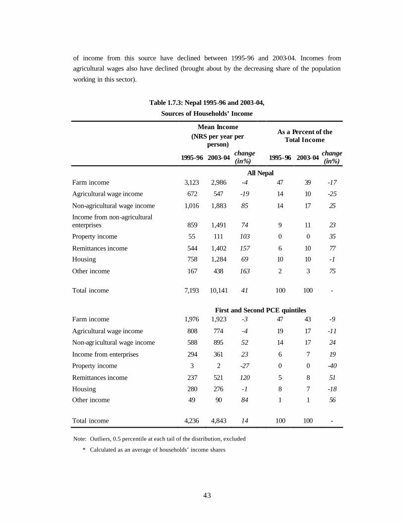
43
of income from this source have declined between 1995-96 and 2003-04. Incomes from agricultural wages also have declined (brought about by the decreasing share of the population
working in this sector).
Table 1.7.3: Nepal 1995-96 and 2003-04,
Sources of Households’ Income
Mean Income
(NRS per year per person)
As a Percent of the Total Income
1995-96 2003-04 change (in%) 1995-96 2003-04
change (in%)
All Nepal Farm income 3,123 2,986 -4 47 39 -17
Agricultural wage income 672 547 -19 14 10 -25
Non-agricultural wage income 1,016 1,883 85 14 17 25
Income from non-agricultural enterprises 859 1,491 74 9 11 23
Property income 55 111 103 0 0 35
Remittances income 544 1,402 157 6 10 77
Housing 758 1,284 69 10 10 -1
Other income 167 438 163 2 3 75 Total income 7,193 10,141 41 100 100 -
First and Second PCE quintiles Farm income 1,976 1,923 -3 47 43 -9
Agricultural wage income 808 774 -4 19 17 -11
Non-agricultural wage income 588 895 52 14 17 24
Income from enterprises 294 361 23 6 7 19
Property income 3 2 -27 0 0 -40
Remittances income 237 521 120 5 8 51
Housing 280 276 -1 8 7 -18
Other income 49 90 84 1 1 56
Total income 4,236 4,843 14 100 100 -
Note: Outliers, 0.5 percentile at each tail of the distribution, excluded
* Calculated as an average of households’ income shares
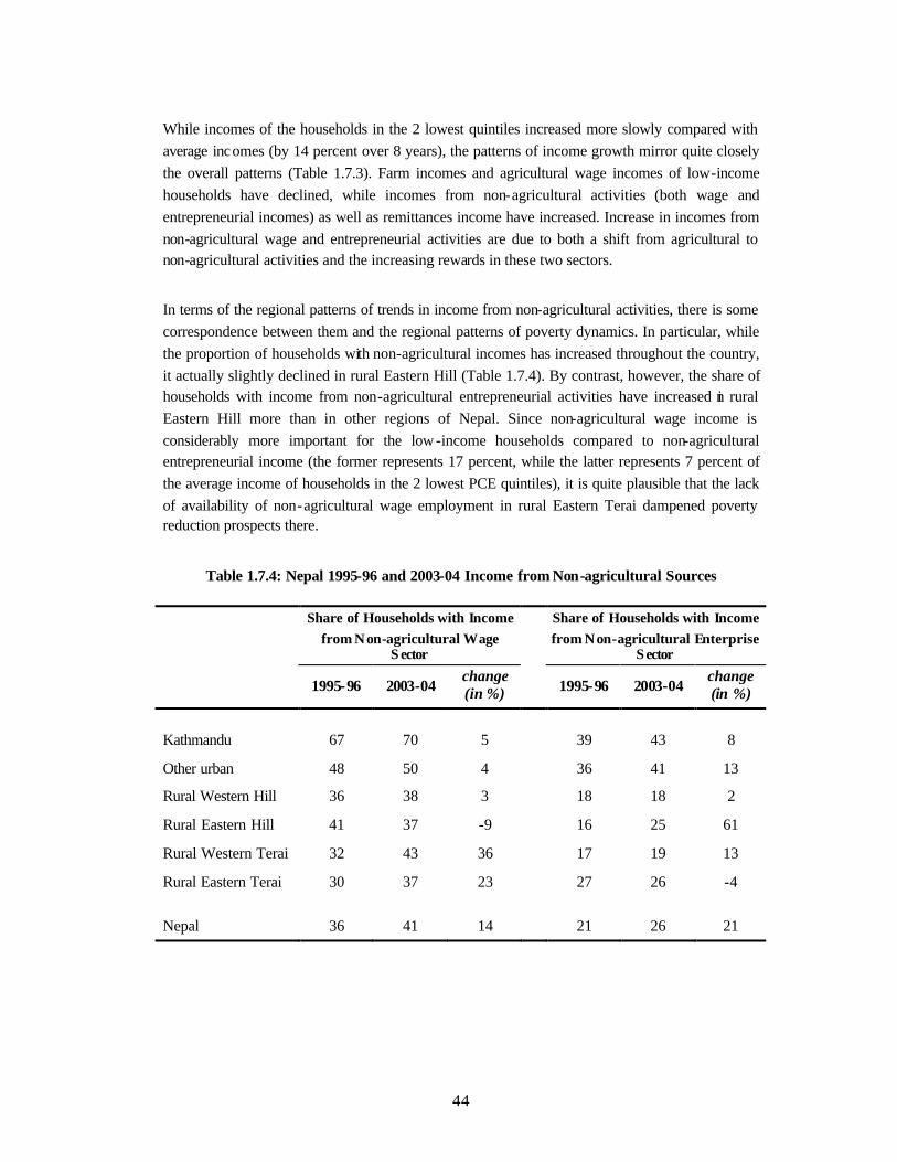
44
While incomes of the households in the 2 lowest quintiles increased more slowly compared with average incomes (by 14 percent over 8 years), the patterns of income growth mirror quite closely the overall patterns (Table 1.7.3). Farm incomes and agricultural wage incomes of low-income households have declined, while incomes from non-agricultural activities (both wage and entrepreneurial incomes) as well as remittances income have increased. Increase in incomes from non-agricultural wage and entrepreneurial activities are due to both a shift from agricultural to non-agricultural activities and the increasing rewards in these two sectors.
In terms of the regional patterns of trends in income from non-agricultural activities, there is some correspondence between them and the regional patterns of poverty dynamics. In particular, while the proportion of households with non-agricultural incomes has increased throughout the country, it actually slightly declined in rural Eastern Hill (Table 1.7.4). By contrast, however, the share of households with income from non-agricultural entrepreneurial activities have increased in rural Eastern Hill more than in other regions of Nepal. Since non-agricultural wage income is considerably more important for the low -income households compared to non-agricultural entrepreneurial income (the former represents 17 percent, while the latter represents 7 percent of the average income of households in the 2 lowest PCE quintiles), it is quite plausible that the lack of availability of non-agricultural wage employment in rural Eastern Terai dampened poverty reduction prospects there.
Table 1.7.4: Nepal 1995-96 and 2003-04 Income from Non-agricultural Sources
Share of Households with Income
from Non-agricultural Wage S ector
Share of Households with Income from Non-agricultural Enterprise
S ector
1995-96 2003-04 change (in %) 1995-96 2003-04
change (in %)
Kathmandu 67 70 5 39 43 8
Other urban 48 50 4 36 41 13
Rural Western Hill 36 38 3 18 18 2
Rural Eastern Hill 41 37 -9 16 25 61
Rural Western Terai 32 43 36 17 19 13
Rural Eastern Terai 30 37 23 27 26 -4
Nepal 36 41 14 21 26 21
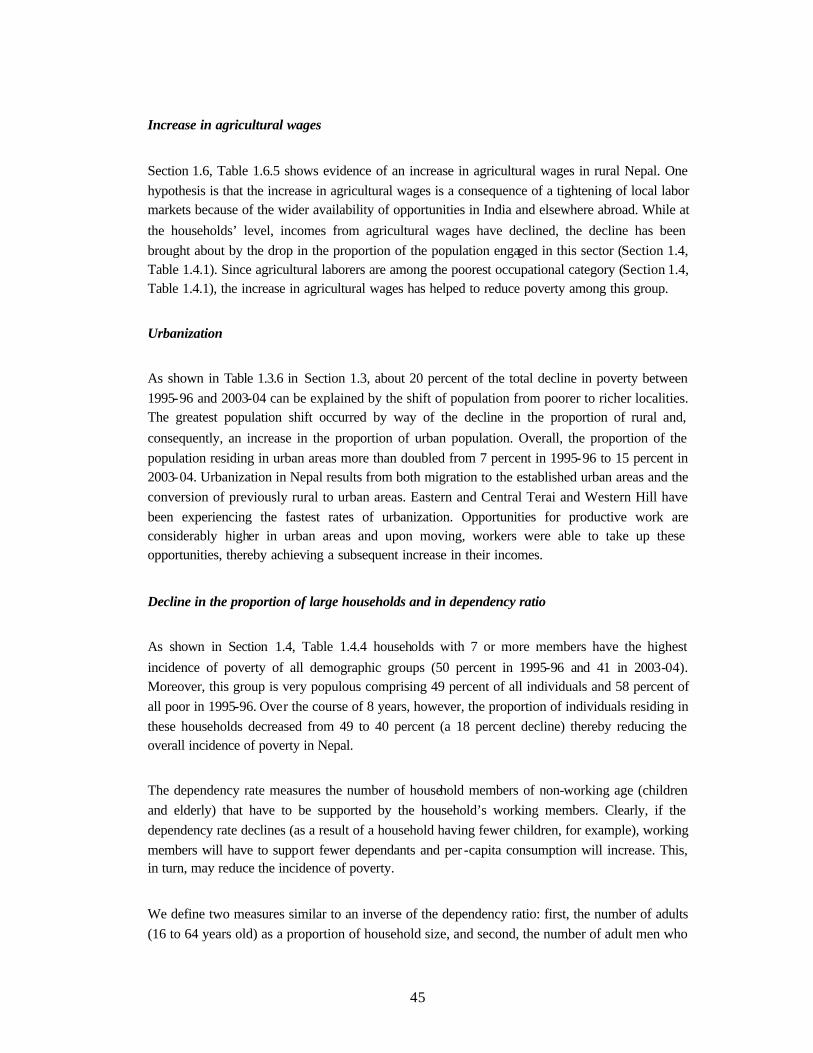
45
Increase in agricultural wages
Section 1.6, Table 1.6.5 shows evidence of an increase in agricultural wages in rural Nepal. One hypothesis is that the increase in agricultural wages is a consequence of a tightening of local labor markets because of the wider availability of opportunities in India and elsewhere abroad. While at the households’ level, incomes from agricultural wages have declined, the decline has been brought about by the drop in the proportion of the population engaged in this sector (Section 1.4, Table 1.4.1). Since agricultural laborers are among the poorest occupational category (Section 1.4, Table 1.4.1), the increase in agricultural wages has helped to reduce poverty among this group.
Urbanization
As shown in Table 1.3.6 in Section 1.3, about 20 percent of the total decline in poverty between 1995-96 and 2003-04 can be explained by the shift of population from poorer to richer localities. The greatest population shift occurred by way of the decline in the proportion of rural and, consequently, an increase in the proportion of urban population. Overall, the proportion of the population residing in urban areas more than doubled from 7 percent in 1995-96 to 15 percent in 2003-04. Urbanization in Nepal results from both migration to the established urban areas and the conversion of previously rural to urban areas. Eastern and Central Terai and Western Hill have been experiencing the fastest rates of urbanization. Opportunities for productive work are considerably higher in urban areas and upon moving, workers were able to take up these opportunities, thereby achieving a subsequent increase in their incomes.
Decline in the proportion of large households and in dependency ratio
As shown in Section 1.4, Table 1.4.4 households with 7 or more members have the highest incidence of poverty of all demographic groups (50 percent in 1995-96 and 41 in 2003-04). Moreover, this group is very populous comprising 49 percent of all individuals and 58 percent of all poor in 1995-96. Over the course of 8 years, however, the proportion of individuals residing in these households decreased from 49 to 40 percent (a 18 percent decline) thereby reducing the overall incidence of poverty in Nepal.
The dependency rate measures the number of household members of non-working age (children and elderly) that have to be supported by the household’s working members. Clearly, if the dependency rate declines (as a result of a household having fewer children, for example), working members will have to support fewer dependants and per -capita consumption will increase. This, in turn, may reduce the incidence of poverty.
We define two measures similar to an inverse of the dependency ratio: first, the number of adults (16 to 64 years old) as a proportion of household size, and second, the number of adult men who
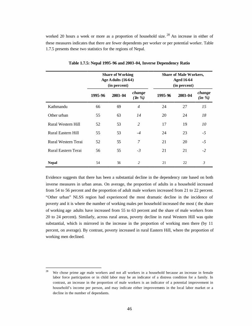
46
worked 20 hours a week or more as a proportion of household size. 28 An increase in either of
these measures indicates that there are fewer dependents per worker or per potential worker. Table 1.7.5 presents these two statistics for the regions of Nepal.
Table 1.7.5: Nepal 1995-96 and 2003-04, Inverse Dependency Ratio
Share of Working Age Adults (16-64)
(in percent)
Share of Male Workers, Aged 16-64 (in percent)
1995-96 2003-04 change (In %) 1995-96 2003-04
change (in %)
Kathmandu 66 69 4 24 27 15
Other urban 55 63 14 20 24 18
Rural Western Hill 52 53 2 17 19 10
Rural Eastern Hill 55 53 -4 24 23 -5
Rural Western Terai 52 55 7 21 20 -5
Rural Eastern Terai 56 55 -3 21 21 -2
Nepal 54 56 2 21 22 3
Evidence suggests that there has been a substantial decline in the dependency rate based on both
inverse measures in urban areas. On average, the proportion of adults in a household increased from 54 to 56 percent and the proportion of adult male workers increased from 21 to 22 percent.
“Other urban” NLSS region had experienced the most dramatic decline in the incidence of poverty and it is where the number of working males per household increased the most ( the share
of working age adults have increased from 55 to 63 percent and the share of male workers from 20 to 24 percent). Similarly, across rural areas, poverty decline in rural Western Hill was quite substantial, which is mirrored in the increase in the proportion of working men there (by 11
percent, on average). By contrast, poverty increased in rural Eastern Hill, where the proportion of working men declined.
28 We chose prime age male workers and not all workers in a household because an increase in female
labor force participation or in child labor may be an indicator of a distress condition for a family. In contrast, an increase in the proportion of male workers is an indicator of a potential improvement in household’s income per person, and may indicate either improvements in the local labor market or a decline in the number of dependants.
47
CHAPTER II
The Methodology used to Derive Poverty Lines (1995-96 and 2003-04)
The main objective of this chapter is to document the main steps and procedures followed by the poverty assessment team to construct poverty lines for the 2003-04 Nepal Living Standards Survey (NLSS II) data sets. In constructing these poverty lines, it is important to highlight upfront that our overriding concern was to maintain comparability with the methodology employed in the 2000 World Bank report “Nepal: Poverty at the Turn of the Twenty-First Century”, that utilized
data from the 1995-96 NLSS (NLSS I). Thus, we have taken the 1995-96 poverty line developed
by the CBN method and derived indices (in case of the NLSS I we re-derived these indices) to adjust it for regional differences in cost-of-living. We also derived region-specific inter-temporal indices. We then used these indices to estimate the cost of poverty lines in 6 regions in 2 time periods. We did not revisit the calculation of the poverty line itself. The main advantage of not
revisiting the calculation of poverty line is to keep the “yardstick” intact, and to preserve the continuity and comparability of the 2003-04 results with the earlier estimates of poverty in Nepal.
This chapter contains four sections which are organized as follows.
Section 2.1 provides a brief, intuitive, and non-technical overview for the non-specialist reader to the methodology followed to derive the poverty lines.
Section 2.2 provides a more detailed account of the specific steps that were followed, and
Section 2.3 presents the various poverty lines for each region-of-interest, which wer e then used to estimate poverty incidence in the country in 1995-96 and 2003-04.
2.1 An Overview of the Methodology
Taking as a starting point the 1995-96 rural Eastern Terai poverty line (denoted P11) derived by the earlier 2000 Poverty Assessment team (henceforth 2000 PA: see Box 2.1 for a summary of how this line was derived), our objective was to construct comparable poverty lines for each of
the six main regions-of-interest,29 and for both survey periods 1995-96 and 2003-04. In other
29 The regions were (1) Kathmandu; (2) other urban areas; (3) Rural West Hills and Mountains (i.e.
Western, Mid-west, and Far-west Development Regions); (4) Rural Eastern and Central Hills and
48
words, our goal was to derive 12 poverty lines (P it: i=1, 2, 3, 4, 5, 6 and t = 1, 2) for each region/time-period, each of which represented exactly the same standard-of-living or welfare, and
differed in rupee terms only to the extent necessary to make allowances for differences in cost-of-living over time and across regions.
Recall that the
poverty line for any given region (in this
case, the rural Eastern Terai region) includes
provision for a
minimum bundle of goods comprising
essential food and non-food items. The
issue of updating P11 across time and space therefore essentially
boils-down to deriving appropriate price indices for these food and non-food
components (i.e. that
take into account intertemporal and spatial prices differences) and then
applying them to the corresponding parts of the poverty line to
derive the P ij for each of the respective 12 domains of interest.
The above overall process was carried out by following three main steps:
Step 1: Derive the spatial and inter-temporal food price indices to ascer tain the corresponding food poverty line components of each of the 12 main domains of interest.
Mountains; (5) Rural western Terai (i.e. the Western, Mid-west, and Far -west Development Regions); and (6) Rural Eastern and Central Terai.
Box 2.1: Deriving the 1995-96 Rural Eastern Terai Poverty Line: A Brief Synopsis
The poverty line for 1995-96 NLSS was derived using the Cost-of-Basic-Needs (CBN) method. In short, the method entailed 5 main steps:
? First, a nutrition norm of per capita 2,124 kcal per day was determined based on the minimum caloric requirements for different age and gender groups and the composition of an “average” Nepali household.
? Second, 37 food items for which units and prices were available were selected and their quantities consumed by the households in the second to fifth decile of per-capita consumption distribution were determined. Expenditure on these 37 goods represented, on average, 85 percent of all food expenditures of households, so it was assumed that these foods provided 85 percent of all requisite caloric requirements. The average actual caloric content of this food bundle was found to be 1,736 kcal. To ensure that the food basket yielded the requisite calories, all quantities were scaled up uniformly by the ratio of 1,805/1,736 (1,805 is 85 percent of 2,124 kcal).
? Third, the cost of this bundle was determined using mean unit values for these goods in rural Eastern Terai region. Unit values were calculated as “plutocratic” averages across the entire population of rural Eastern Terai. This basket turned out to cost Rs. 2,647 per person per annum.
? Fourth, assuming that all other foods have the same price per calorie, the food basket that would provide 100 percent caloric requirement would cost 15 percent more or Rs 3,114.1per person per annum.
? Fifth, the final step was to determine the share of non-food consumption of the households whose food consumption was around the requisite food poverty line (i.e. the upper poverty line in the terminology of Ravallion 2000). Adding the average amount for non-food items (Rs. 1,540.5), the final poverty line was calculated as Rs 4,654.6 per person per annum in rural Eastern Terai prices.
See Lanjouw, Prennushi and Zaidi (1999) “Poverty in Nepal Today” for more details
49
Step 2: Derive the spatial and inter -temporal non-food price indices for the corresponding non-food poverty line components of each of the 12 main domains of interest.
Step 3: Aggregate the food and non-food poverty line components to obtain the respective Pij i.e. the 12 overall poverty lines of interest.
Having thus determined the overall total poverty lines in prices of the six regions -of-interest in 1995-96 and 2003-04, we then compared them with nominal consumption aggregates derived from the survey data to categorize the population into poor and non-poor group.
2.2 Deriving the Poverty Lines: A more Detailed Exposition 30
Following the brief outline above of the steps followed to construct the 12 poverty lines of interest; this section provides a more thorough account of the procedures followed in deriving the poverty lines. While steps 1 and 2 outlined above could in-principle have been combined by
deriving a composite price index for the food and non-food bundles taken together,31 we instead derived these two sets of price indices separately, and then applied these to the food and non-food components of the poverty line respectively to eventually arrive at the overall poverty lines for the
12 domains. The exact steps followed in carrying out these procedures are elaborated below.
2.2.1 Deriving the Food Price Indices
In deriving price indices to update poverty lines, literature on this topic suggests an estimation strategy that (i) utilizes prices faced by the poor, and (ii) uses quantities consumed (or budget
shares) that are aligned with the consumption patterns of the poor. In particular, several authors (recently Deaton and Tarozzi) suggest deriving both quantities and unit values of consumed foods 30 An alternative approach for deriving the poverty lines for 2003-04 would be to use the same
methodology as in 1995-96 to compute poverty lines in 2003 -04. However, this approach is not well-suited for inter-temporal comparisons: a major drawback is that if living standards in a country improve
over time, even poor households improve the composition of their consumption basket. As a result,
reapplying the CBN methodology poverty lines therefore no longer reflect basic-needs bundles of
constant value in real terms. Assessing trends in absolute poverty over time presumes that the same yardstick was used at all points in time, a condition that is violated by the application of the same
methodology to the derivation of poverty line in 2003-04. See Ravallion Martin (1994) Poverty
Comparisons Hardwood Academic Press, Switzerland, for a discussion of these issues.
31 Indeed, this was the procedure followed in the earlier Poverty Assessment; however, since we departed from this earlier practice, the poverty lines derived in this paper for the five other regions (i.e. other
than the rural Eastern Terai) are in -fact slightly different from those used for the earlier Poverty Assessment.
50
from the household survey(s) data to form baskets of consumer goods in different locations (time periods), which in turn are then used to derive the food price indices.32
We calculated food prices indices in the 12 domains of interest using a Laspeyres index—i.e. as the relative costs of the 1995-96 fixed food basket in two time periods and across the 6 main regions of interest. We chose Laspeyres index for two main reasons: (i) to maintain comparability with earlier analysis (i.e. in the 2000 PA), and (ii) this index (which is constructed in such a way that weights attached to each food item are the same for all regions and time periods) satisfies base-independency and transitivity properties, in other words the relative prices across regions and time periods do not depend on the choice of the base-region, or the sequence in which spatial and inter -temporal indices are combined. 33
To construct the Laspeyres index, the quantities of 37 food items for a fixed food basket were chosen using the 1995-96 national average quantities consumed by the population in the 2nd to 5th deciles of nominal per capita consumption. 34 The region and time period-specific prices of each
32 See Deaton and Tarozzi “Prices and Poverty in India” in The Great Indian Poverty Debate, A. Deaton
and Valerie Kozel eds.. This paper also provide guidance on methodology for calculating unit values and quantities and on the merits of selecting particular price indices -- Laspeyres, Paasche, Tornquist,
Fisher, etc.
33 The Laspeyres index also has its disadvantages vis-à-vis such superlative indices as Tornquist and
Fisher, the main disadvantage being that it is not derived from a demand system or an expenditure
function. Unfortunately, however, superlative indices are not transitive and in case of multilateral (i.e.,
across space and time) comparisons the result depend on the order by which regional and intertemporal indices are combined. For instance, when calculating the relative price difference between Kathmandu in 1995-96 and rural East Hill (REH) in 2003-04 one would want the result to be the independent of
whether one first applies regional price index to convert 1995-96 Kathmandu prices to 1995 -96 REH
prices and then intertemporal index to convert 1995-96 REH prices to 2003-04 REH prices, versus when one first applies intertemporal price index to convert 1995 -96 Kathmandu prices to 2003 -04
Kathmandu prices, and then regional price index to convert 2003-04 Kathmandu prices to the 2003 -04
REH prices. If one adopts Tornquist or Fisher indexes, these procedures give different results,
depending on the order followed. This lack of transitivity of superlative indices could also be understood in terms of base-dependency or the dependency of the relative prices on the choice of a
base region. In this case, if one were to use superlative indices, the relative prices would’ve depended
on the choice of a base region, be it Kathmandu, Rural East Hills or the other region.
34 The quantities were calculated as “democratic” rather than “plutocratic” means; the difference between
the two is that the latter uses aggregate consumers’ expenditure on each commodity divided by the
aggregate consumers’ expenditure on all commodities which is an average of the individual households ratios weighted by the total expenditure. As a result, “plutocratic” average gives bigger weight to
households which consume more of a particular product (usually richer households). Democratic method is preferred for calculating price indexes faced by the poor, as it places equal weights on
consumption of each household, irrespective of the quantity consumed. See Deaton and Tarozzi 2000 “Prices and Poverty in India” for a more detailed discussion of these two methods.

51
food item were calculated as the average “democratic” unit values taken over the entire population of that region in 1995-96 and in 2003-04. 35 To obtain total quantities, quantities of purchased, home-produced and received-in-kind food were added up for each household and food item. Technical details regarding treatment of purchased, home-produced and received-in-kind items, as well as issues pertaining to conversion of non-metric units, are discussed in Annex 2.
Computed quantities and prices were checked for the presence of outliers, which were subsequently removed from the analysis. In addition, a household-level unit value was considered to be an outlier if it was either less then 0.1 times or greater than 10 times the median unit value of a particular food item. The cost of each basket was computed as the sum of expenditures on each food from the food basket, using the region and time period-specific prices. Results are presented in Table 2.3.1.
Table 2.2.1: Nepal 1995-96 and 2003-04, Regional Food Price Indices
Cost of a Reference Food Basket (in current local
prices)
Implied Food Poverty Line adjustment
coefficient 1995-96 2003-04 1995-96 2003-04
Implied region-specific food inflation rate
(1) (2) (3) (4) (5)
Kathmandu 3,361 5,550 1.29 2.14 165.1
Other urban 2,950 4,062 1.14 1.56 137.7
Rural Western Hill 3,178 4,634 1.22 1.79 145.8
Rural Eastern Hill 3,289 4,385 1.27 1.69 133.3
Rural Western Terai 2,458 3,557 0.95 1.37 144.7
Rural Eastern Terai 2,596 3,570 1.00 1.38 137.5
All-Nepal 2,908 4,101 1.12 1.58 141.0
* Column 5 is calculated as column 4 divided by column 3, multiplied by 100
As a cross-check, we compared inter -temporal change in prices calculated from the survey data with the official CPIs. According to the Rastra Bank, the urban CPI for “food and beverages” in 2003-04 was 148.8 compared to 100 in 1995-96 (i.e. 1995-96 is the base year for the urban CPI). The NLSS-based estimated all-Nepal food price index is 141.0, or quite comparable to the official
CPI estimate (that it is slightly on the lower side could be explained by the fact that the NLSS-based estimates are heavily drawn from the rural areas, and are based on foods generally consumed by the poor).
35 It would’ve been preferable to take prices faced by the “poor” and calculate unit values only over the
population in the 2-5 deciles. But since these calculations had to be done at the regional level, the sample sizes were too small.
52
2.2.2 Deriving the Non-Food Price Indices
In case of non food price indices, we estimated relative costs of renting a typical housing unit to account for regional differences in prices, but used the urban CPI collected by the Rastra Bank to
approximate the inter-temporal change in non-food prices. We believe that while differences in rental values are reasonable proxies for regional differences in price level, inter-temporal changes in rental prices are a poor approximation for the changes in non food prices.36 This is because the inter-temporal trajectory of prices of non-food items (mostly services and tradable goods) is also
influenced by changes in world prices (most notably, the prices of fuel) and changes in the
demand and supply of these goods and services; changes in the price of rental housing is a poor proxy for such price changes.37 We therefore used a combination of a single inter-temporal non-
food all urban Nepal CPI provided by the Rastra Bank and regional housing price indices calculated on the basis of NLSS 2003-04 survey. 38 Details pertaining to how this procedure was
implemented are provided below.
Similar to calculation of non-food price indices by the 2000 PA team for the 1995-96 survey, we calculated the cost of renting a reference house (an average house in terms of facilities affecting
rent) in 6 regions in 2003-04. The cost function was estimated using a hedonic housing regression model to predict the rental values for those households in the sample that had not paid rents (the similar model was estimated to infer housing consumption in the construction of consumption
aggregates). We then calculated regional non-food price indices both in 1995-96 and in 2003-04 relative to the year-specific Rural Eastern Terai prices (Table 2.2.2, columns 2 and 5).
36 Bangladesh Poverty Assessment (2002) used a similar approach of combining a survey-based index
and an official CPI into an overall price index. Since regional non-food CPIs were available for Bangladesh, these indices were used to approximate both regional and inter-temporal differences of the non-food items.
37 On examination of the data, we found that survey -based estimates of change in the housing prices showed a considerably smaller increase than the increase in prices of several non-food items that were also collected in the survey. For example, in rural Eastern Terai the NLSS-based rental housing prices had actually declined, even in nominal terms. By contrast, the increase in prices of kerosene and chappals (footwear) show increases comparable with the increase in the urban non-food CPI.
38 Alternatively, we could have applied the average inter -temporal price index to the regional price indices in 1995-96. This method, however, would’ve imposed the regional differences prevailing in 1995-96 onto the 2003-04 regional indexes. We believe our method which actually estimates the regional price difference in 2003-04 is a superior one.
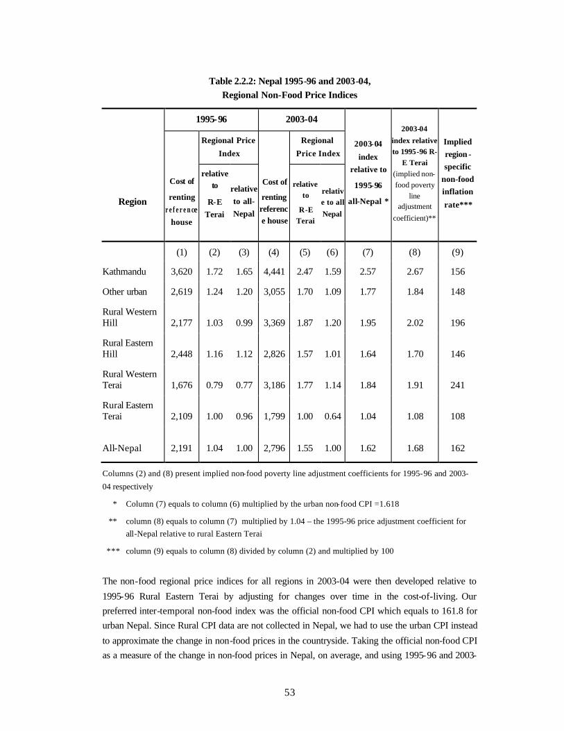
53
Table 2.2.2: Nepal 1995-96 and 2003-04, Regional Non-Food Price Indices
1995-96 2003-04
Regional Price
Index
Regional
Price Index
Region
Cost of
renting r e f e r e n ce
house
relative to
R-E Terai
relative to all-Nepal
Cost of
renting reference house
relative to
R-E Terai
relative to all Nepal
2003-04
index relative to
1995-96
all-Nepal *
2003-04 index relative to 1995-96 R-
E Terai (implied non-food poverty
line adjustment
coefficient)**
Implied region - specific
non-food inflation
rate***
(1) (2) (3) (4) (5) (6) (7) (8) (9)
Kathmandu 3,620 1.72 1.65 4,441 2.47 1.59 2.57 2.67 156
Other urban 2,619 1.24 1.20 3,055 1.70 1.09 1.77 1.84 148
Rural Western Hill 2,177 1.03 0.99 3,369 1.87 1.20 1.95 2.02 196
Rural Eastern Hill 2,448 1.16 1.12 2,826 1.57 1.01 1.64 1.70 146
Rural Western Terai 1,676 0.79 0.77 3,186 1.77 1.14 1.84 1.91 241
Rural Eastern Terai 2,109 1.00 0.96 1,799 1.00 0.64 1.04 1.08 108
All-Nepal 2,191 1.04 1.00 2,796 1.55 1.00 1.62 1.68 162
Columns (2) and (8) present implied non-food poverty line adjustment coefficients for 1995-96 and 2003-
04 respectively
* Column (7) equals to column (6) multiplied by the urban non-food CPI =1.618
** column (8) equals to column (7) multiplied by 1.04 – the 1995-96 price adjustment coefficient for all-Nepal relative to rural Eastern Terai
*** column (9) equals to column (8) divided by column (2) and multiplied by 100
The non-food regional price indices for all regions in 2003-04 were then developed relative to
1995-96 Rural Eastern Terai by adjusting for changes over time in the cost-of-living. Our preferred inter-temporal non-food index was the official non-food CPI which equals to 161.8 for urban Nepal. Since Rural CPI data are not collected in Nepal, we had to use the urban CPI instead
to approximate the change in non-food prices in the countryside. Taking the official non-food CPI as a measure of the change in non-food prices in Nepal, on average, and using 1995-96 and 2003-
54
04 regional differences in costs of rental housing as regional non-food price indices in respective time periods, we then calculated the region-specific inter -temporal change in non-food prices, and
then further the changes in non-food prices relative to 1995-96 rural Eastern Terai.39 Specifically, first, we calculated change in prices in all regions in 2003-04 relative to 1995-96 Nepal average. Second, knowing the ratio of rural Eastern Terai prices in 1995-96 to the average Nepal prices in 1995-96, we re-calculated all requisite price indices relative to the 1995-96 rural Eastern Terai
(which were needed to adjust the poverty line).40 Table 2.2.2 presents all resulting coefficients.
2.2.3 Aggregating the Food and Non-food Poverty Line Components
Once regional and inter -temporal food and non-food indices (Table 2.2.1 columns 3 and 4, and Table 2.2.2 columns 2 and 8, respectively) had been calculated, we applied these to the
corresponding parts of the 1995-96 Rural Eastern Terai poverty line (i.e. P11) in order to derive the
other poverty lines (i.e. Pit). However, before this last step could be carried out, we made one more adjustment in the case of the 2003-04 poverty lines to take into account the change in
demographic composition of the population between 1995-96 and 2003-04 (see Box 2.2).
39 Note that it is important to maintain that the average Nepal non-food prices increased by 61.8 percent;
it would be questionable to assume that the rural Eastern Terai non-food prices had increased by that
much and then infer changes in prices between the 6 regions in 2003-04 and rural Eastern Terai in
1995-96 on the basis of this coefficient and 2003 -04 regional differentials. More discussion about
combining regional and inter-temporal indexes is presented in Hill, Robert J. 2004 “Constructing Price
Indexes Across Space and Time: The case of the European Union”, The American Economic Review,
Vol. 94, Number 5.
40 The following example will further clarify the procedure implemented. Let us say one wants to express
prices in Kathmandu in 2003-04 relative to prices in rural Eastern Terai in 1995-96, provided that the
average inflation between 1995-96 and 2003-04 was 1.618. One needs to multiply 1.59 (which is an
index of relative prices in Kathmandu in 2003-04 relative to all-Nepal average in that year, column 6,
Table 3.2) by 1.618 (average inflation index) which will give a change in price in Kathmandu in 2003-
04 relative to 1995 -96 average Nepal prices (column 7, Table 2.3.2).The next step is to divide this number by 0.96 (the index of relative prices in rural Eastern Terai in 1995-96 relative to all-Nepal
average prices in that year) to obtain the requisite relative price index (column 8, Table 2.3.2). One can
see then that prices in Kathmandu in 2003-04 were 2.67 times higher than prices in rural East Terai in
1995-96.
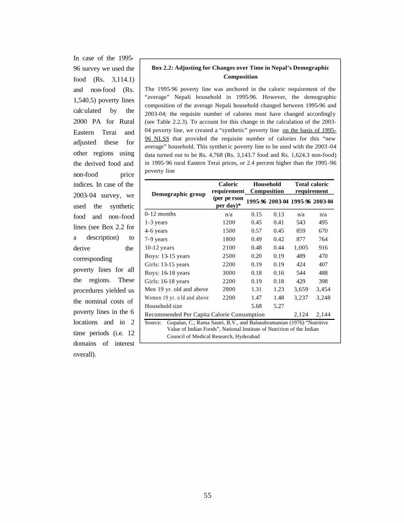
55
In case of the 1995-96 survey we used the
food (Rs. 3,114.1) and non-food (Rs. 1,540.5) poverty lines calculated by the
2000 PA for Rural
Eastern Terai and adjusted these for
other regions using the derived food and
non-food price indices. In case of the
2003-04 survey, we
used the synthetic food and non-food lines (see Box 2.2 for a description) to
derive the corresponding
poverty lines for all the regions. These procedures yielded us
the nominal costs of poverty lines in the 6 locations and in 2
time periods (i.e. 12 domains of interest
overall).
Box 2.2: Adjusting for Changes over Time in Nepal’s Demographic Composition
The 1995-96 poverty line was anchored in the caloric requirement of the “average” Nepali household in 1995-96. However, the demographic composition of the average Nepali household changed between 1995-96 and 2003-04; the requisite number of calories must have changed accordingly (see Table 2.2.3). To account for this change in the calculation of the 2003-04 poverty line, we created a “synthetic” poverty line on the basis of 1995-96 NLSS that provided the requisite number of calories for this “new average” household. This synthet ic poverty line to be used with the 2003 -04 data turned out to be Rs. 4,768 (Rs. 3,143.7 food and Rs. 1,624.3 non-food) in 1995-96 rural Eastern Terai prices, or 2.4 percent higher than the 1995 -96 poverty line
Household Composition
Total caloric requirement Demographic group
Caloric requirement (per pe rson per day)*
1995-96 2003-04 1995-96 2003-04
0-12 months n/a 0.15 0.13 n/a n/a 1-3 years 1200 0.45 0.41 543 495 4-6 years 1500 0.57 0.45 859 670 7-9 years 1800 0.49 0.42 877 764 10-12 years 2100 0.48 0.44 1,005 916 Boys: 13-15 years 2500 0.20 0.19 489 470 Girls: 13-15 years 2200 0.19 0.19 424 407 Boys: 16-18 years 3000 0.18 0.16 544 488 Girls: 16-18 years 2200 0.19 0.18 429 398 Men 19 yr. old and above 2800 1.31 1.23 3,659 3,454 Women 19 yr. o ld and above 2200 1.47 1.48 3,237 3,248 Household size 5.68 5.27 Recommended Per Capita Calorie Consumption 2,124 2,144 Source: Gopalan, C., Rama Sastri, B.V., and Balasubramanian (1976) “Nutritive
Value of Indian Foods”, National Institute of Nutrition of the Indian Council of Medical Research, Hyderabad

56
2.3 Region and Time-Specific Poverty Lines and Overall Price Index
The resultant poverty lines are presented in Table 2.3.1. Subsequently, consumption of various goods and services (food, housing, stream of services from durables, etc.) in the last 12 months was added up for every household to arrive at total household expenditure. 41 Per capita expenditure (PCE) was then defined by dividing the total consumption by the household size. 42 These consumption aggregates were then compared with the derived nominal poverty lines (Table 2.3.1: columns 3 and 6) to infer whether a household should be deemed poor or non-poor.
Table 2.3.1: Nepal 1995-96 and 2003-04,
Poverty Lines in Current Prices per Person per Year
1995-96 2003-04
Food Non-Food Total Food Non-food Total
(1) (2) (3) (4) (5) (6)
Kathmandu 4,032.5 2,643.4 6,675.9 6,722.0 4,334.8 11,056.8
Other urban 3,539.2 1,912.6 5,451.8 4,919.2 2,981.9 7,901.1
Rural Western Hill
3,813.0 1,590.0 5,403.0 5,613.0 3,288.5 8,901.5
Rural Eastern Hill 3,946.1 1,787.9 5,734.0 5,311.2 2,758.5 8,069.6
Rural Western Terai
2,949.5 1,223.9 4,173.4 4,308.4 3,110.0 7,418.4
Rural Eastern Terai
3,114.1 1,540.5 4,654.6 4,323.2 1,755.6 6,078.8
All-Nepal 3,488.9 1,599.8 5,088.7 4,966.4 2,729.4 7,695.7
Note: columns 1, 2 and 3 are based in the 1995-96 poverty line; columns 4, 5, and 6 are based on 1995-
96 synthetic poverty line – i.e., are adjusted for the change in the demographic composition of an “average” household (see Box 2.2 for details).
41 Aggregation methodology is based on gu idelines in Deaton and Zaidi (2002): World Bank Living
Standards Survey Working Paper #135 “Guidelines for Constructing Consumption Aggregates for Welfare Analysis"
42 A detailed description of the construction of consumption aggregates is presented in “Nepal Living Standards Survey” Volume 2, Central Bureau of Statistics, HMGN, 2004.
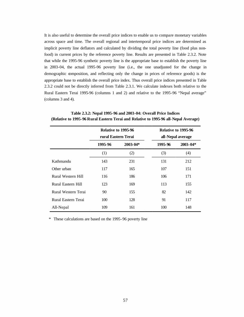
57
It is also useful to determine the overall price indices to enable us to compare monetary variables across space and time. The overall regional and intertemporal price indices are determined as
implicit poverty line deflators and calculated by dividing the total poverty line (food plus non-food) in current prices by the reference poverty line. Results are presented in Table 2.3.2. Note that while the 1995-96 synthetic poverty line is the appropriate base to establish the poverty line in 2003-04, the actual 1995-96 poverty line (i.e., the one unadjusted for the change in
demographic composition, and reflecting only the change in prices of reference goods) is the
appropriate base to establish the overall price index. Thus overall price indices presented in Table 2.3.2 could not be directly inferred from Table 2.3.1. We calculate indexes both relative to the
Rural Eastern Terai 1995-96 (columns 1 and 2) and relative to the 1995-96 “Nepal average” (columns 3 and 4).
Table 2.3.2: Nepal 1995-96 and 2003-04: Overall Price Indices (Relative to 1995-96 Rural Eastern Terai and Relative to 1995-96 all-Nepal Average)
Relative to 1995-96
rural Eastern Terai
Relative to 1995-96
all-Nepal average
1995-96 2003-04* 1995-96 2003-04*
(1) (2) (3) (4)
Kathmandu 143 231 131 212
Other urban 117 165 107 151
Rural Western Hill 116 186 106 171
Rural Eastern Hill 123 169 113 155
Rural Western Terai 90 155 82 142
Rural Eastern Terai 100 128 91 117
All-Nepal 109 161 100 148
* These calculations are based on the 1995-96 poverty line
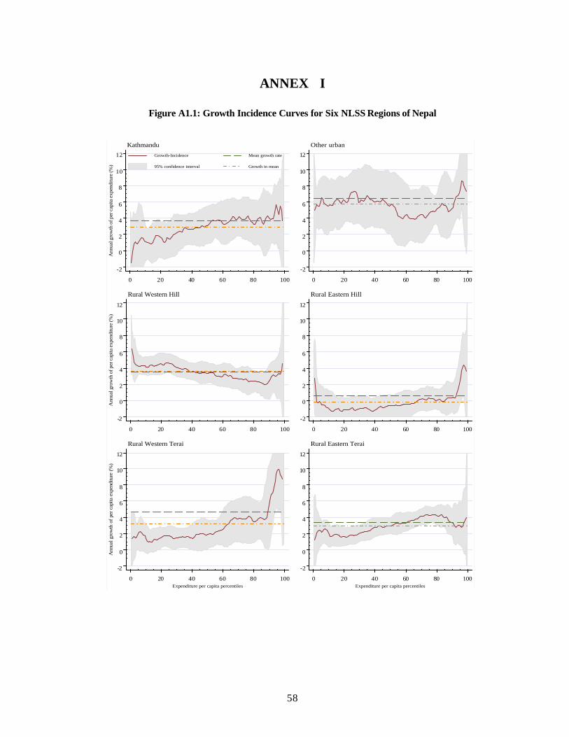
58
-2
0
2
4
6
8
10
12
Ann
ual g
row
th o
f per
cap
ita e
xpen
ditu
re (%
)
0 20 40 60 80 100
Growth-Incidence Mean growth rate
95% confidence interval Growth in mean
Kathmandu
-2
0
2
4
6
8
10
12
0 20 40 60 80 100
Other urban
-2
0
2
4
6
8
10
12
Ann
ual g
row
th o
f per
cap
ita e
xpen
ditu
re (%
)
0 20 40 60 80 100
Rural Western Hill
-2
0
2
4
6
8
10
12
0 20 40 60 80 100
Rural Eastern Hill
-2
0
2
4
6
8
10
12
Ann
ual g
row
th o
f pe
r ca
pita
exp
endi
ture
(%
)
0 20 40 60 80 100Expenditure per capita percentiles
Rural Western Terai
-2
0
2
4
6
8
10
12
0 20 40 60 80 100Expenditure per capita percentiles
Rural Eastern Terai
ANNEX I
Figure A1.1: Growth Incidence Curves for Six NLSS Regions of Nepal
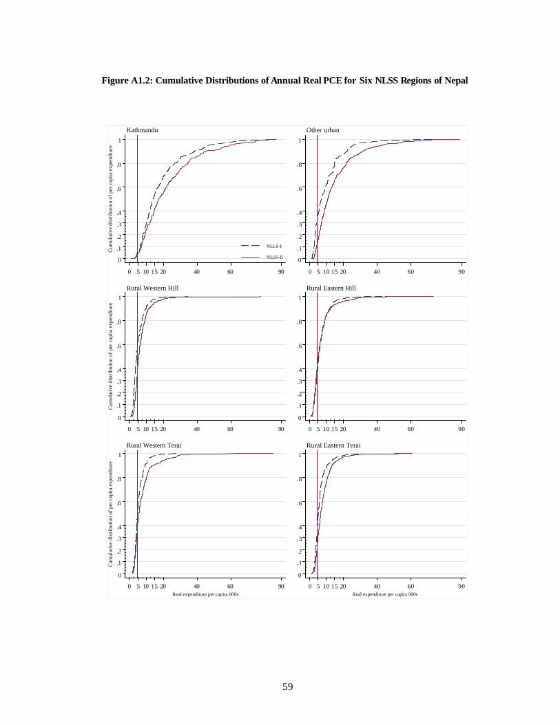
59
Figure A1.2: Cumulative Distributions of Annual Real PCE for Six NLSS Regions of Nepal
0
.1
.2
.3
.4
.6
.8
1
Cum
ulat
ive
dist
ribu
tion
of p
er c
apita
exp
endi
ture
0 20 40 60 905 10 15
NLLS-I
NLSS-II
Kathmandu
0
.1
.2
.3
.4
.6
.8
1
0 20 40 60 905 10 15
Other urban
0
.1
.2
.3
.4
.6
.8
1
Cum
ulat
ive
dist
ribu
tion
of p
er c
apita
exp
endi
ture
0 20 40 60 905 10 15
Rural Western Hill
0
.1
.2
.3
.4
.6
.8
1
0 20 40 60 905 10 15
Rural Eastern Hill
0
.1
.2
.3
.4
.6
.8
1
Cum
ulat
ive
dist
ribut
ion
of p
er c
apita
exp
endi
ture
0 20 40 60 905 10 15Real expenditure per capita 000s
Rural Western Terai
0
.1
.2
.3
.4
.6
.8
1
0 20 40 60 905 10 15Real expenditure per capita 000s
Rural Eastern Terai
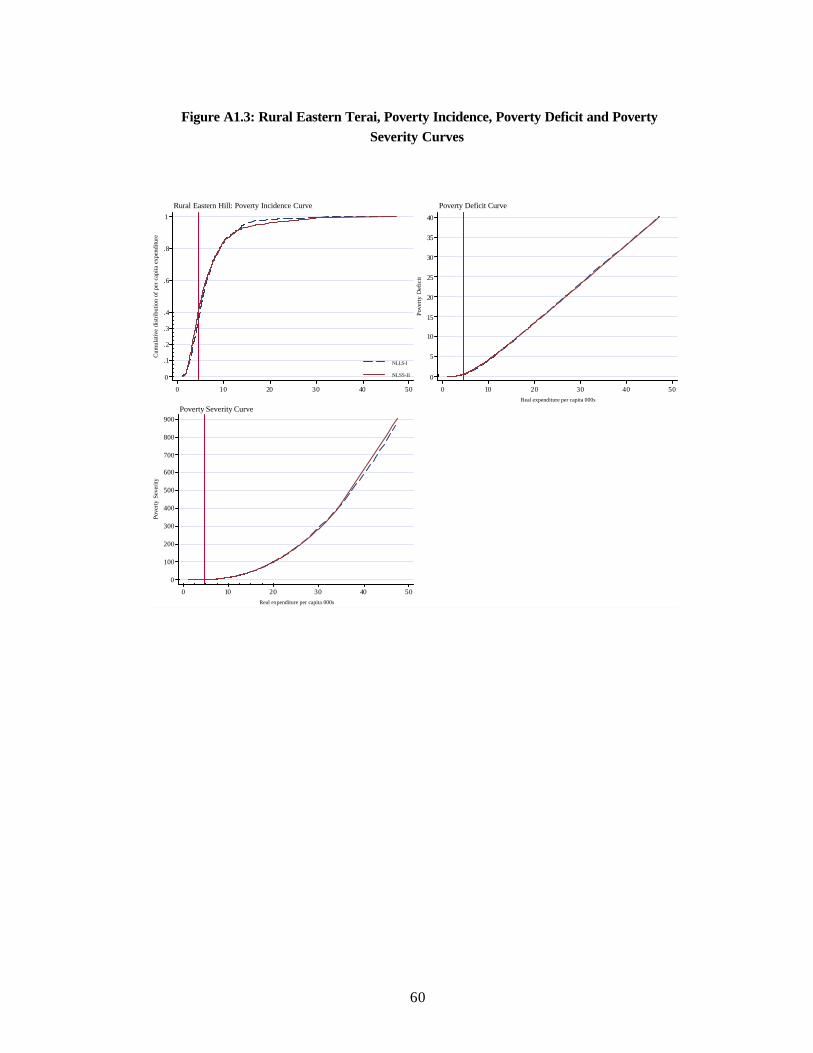
60
0
.1
.2
.3
.4
.6
.8
1
Cum
ulat
ive
dist
ribut
ion
of p
er c
apita
exp
endi
ture
0 10 20 30 40 50
NLLS-I
NLSS-II
Rural Eastern Hill: Poverty Incidence Curve
0
5
10
15
20
25
30
35
40
Pove
rty
Def
icit
0 10 20 30 40 50Real expenditure per capita 000s
Poverty Deficit Curve
0
100
200
300
400
500
600
700
800
900
Pove
rty S
ever
ity
0 10 20 30 40 50Real expenditure per capita 000s
Poverty Severity Curve
Figure A1.3: Rural Eastern Terai, Poverty Incidence, Poverty Deficit and Poverty Severity Curves
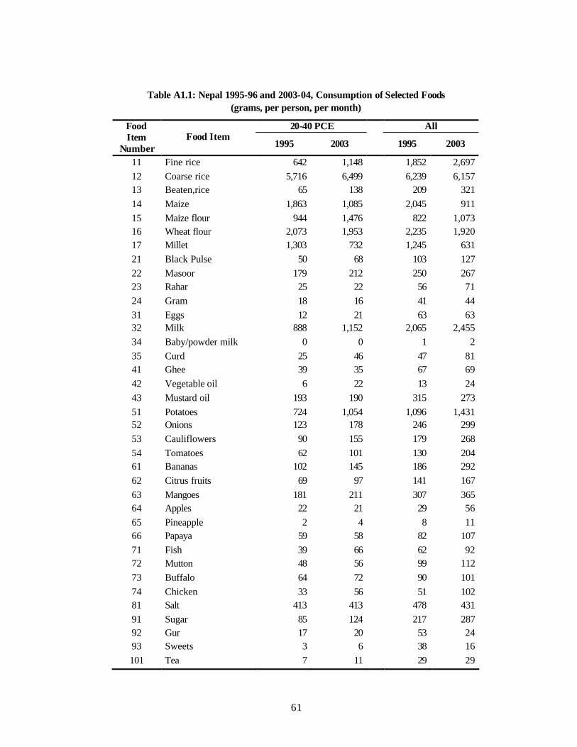
61
Table A1.1: Nepal 1995-96 and 2003-04, Consumption of Selected Foods
(grams, per person, per month)
20-40 PCE All Food Item
Number Food Item
1995 2003 1995 2003
11 Fine rice 642 1,148 1,852 2,697 12 Coarse rice 5,716 6,499 6,239 6,157 13 Beaten,rice 65 138 209 321 14 Maize 1,863 1,085 2,045 911 15 Maize flour 944 1,476 822 1,073 16 Wheat flour 2,073 1,953 2,235 1,920 17 Millet 1,303 732 1,245 631 21 Black Pulse 50 68 103 127 22 Masoor 179 212 250 267 23 Rahar 25 22 56 71 24 Gram 18 16 41 44 31 Eggs 12 21 63 63 32 Milk 888 1,152 2,065 2,455 34 Baby/powder milk 0 0 1 2 35 Curd 25 46 47 81 41 Ghee 39 35 67 69 42 Vegetable oil 6 22 13 24 43 Mustard oil 193 190 315 273 51 Potatoes 724 1,054 1,096 1,431 52 Onions 123 178 246 299 53 Cauliflowers 90 155 179 268 54 Tomatoes 62 101 130 204 61 Bananas 102 145 186 292 62 Citrus fruits 69 97 141 167 63 Mangoes 181 211 307 365 64 Apples 22 21 29 56 65 Pineapple 2 4 8 11 66 Papaya 59 58 82 107 71 Fish 39 66 62 92 72 Mutton 48 56 99 112 73 Buffalo 64 72 90 101 74 Chicken 33 56 51 102 81 Salt 413 413 478 431 91 Sugar 85 124 217 287 92 Gur 17 20 53 24 93 Sweets 3 6 38 16 101 Tea 7 11 29 29
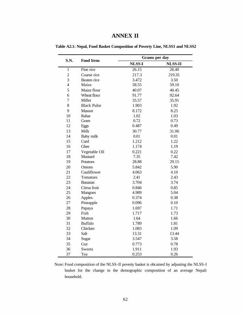
62
ANNEX II
Table A2.1: Nepal, Food Basket Composition of Poverty Line, NLSS1 and NLSS2
Grams per day S.N. Food Item
NLSS-I NLSS-II 1 Fine rice 26.15 26.40 2 Coarse rice 217.3 219.35 3 Beaten rice 3.472 3.50 4 Maize 58.55 59.10 5 Maize flour 40.07 40.45 6 Wheat flour 91.77 92.64 7 Millet 35.57 35.91 8 Black Pulse 1.903 1.92 9 Masoor 8.172 8.25 10 Rahar 1.02 1.03 11 Gram 0.72 0.73 12 Eggs 0.487 0.49 13 Milk 30.77 31.06 14 Baby milk 0.01 0.01 15 Curd 1.212 1.22 16 Ghee 1.174 1.19 17 Vegetable Oil 0.221 0.22 18 Mustard 7.35 7.42 19 Potatoes 28.88 29.15 20 Onions 5.842 5.90 21 Cauliflower 4.063 4.10 22 Tomatoes 2.41 2.43 23 Bananas 3.704 3.74 24 Citrus fruit 0.846 0.85 25 Mangoes 4.989 5.04 26 Apples 0.374 0.38 27 Pineapple 0.096 0.10 28 Papaya 1.697 1.71 29 Fish 1.717 1.73 30 Mutton 1.64 1.66 31 Buffalo 1.789 1.81 32 Chicken 1.083 1.09 33 Salt 13.31 13.44 34 Sugar 3.547 3.58 35 Gur 0.773 0.78 36 Sweets 1.911 1.93 37 Tea 0.253 0.26
Note: Food composition of the NLSS-II poverty basket is obtained by adjusting the NLSS-I basket for the change in the demographic composition of an average Nepali household.
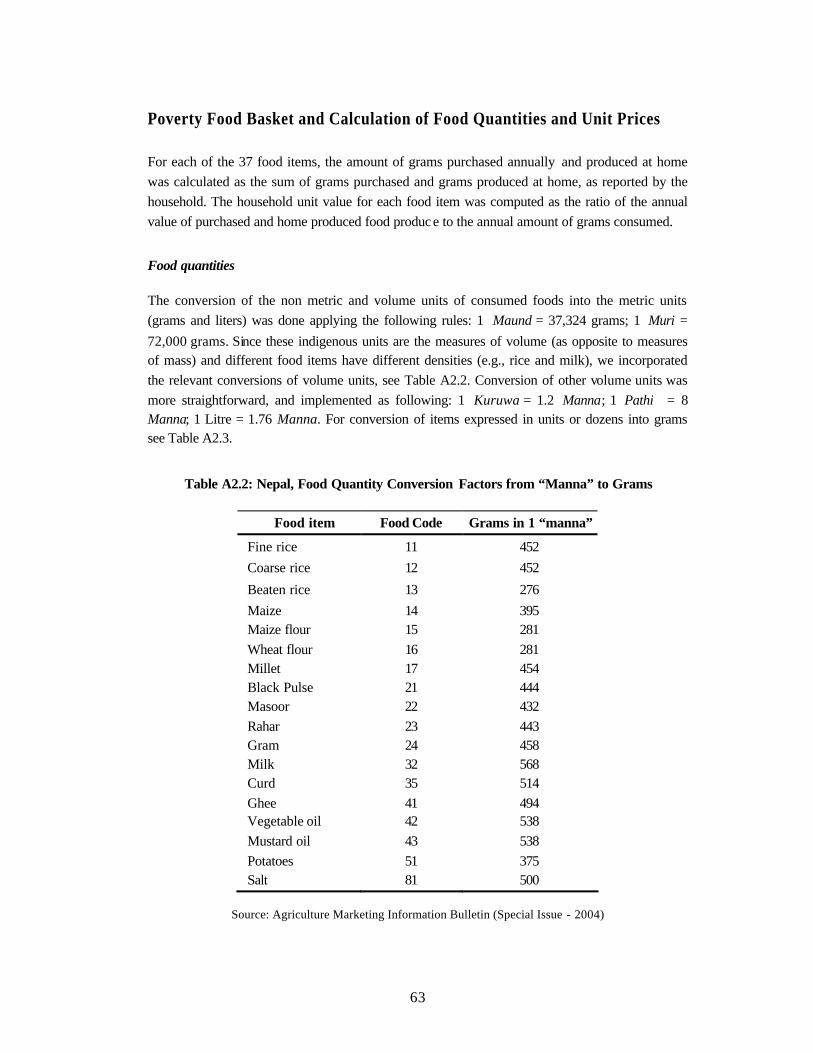
63
Poverty Food Basket and Calculation of Food Quantities and Unit Prices
For each of the 37 food items, the amount of grams purchased annually and produced at home was calculated as the sum of grams purchased and grams produced at home, as reported by the household. The household unit value for each food item was computed as the ratio of the annual value of purchased and home produced food produce to the annual amount of grams consumed.
Food quantities
The conversion of the non metric and volume units of consumed foods into the metric units (grams and liters) was done applying the following rules: 1 Maund = 37,324 grams; 1 Muri = 72,000 grams. Since these indigenous units are the measures of volume (as opposite to measures of mass) and different food items have different densities (e.g., rice and milk), we incorporated the relevant conversions of volume units, see Table A2.2. Conversion of other volume units was more straightforward, and implemented as following: 1 Kuruwa = 1.2 Manna; 1 Pathi = 8 Manna; 1 Litre = 1.76 Manna. For conversion of items expressed in units or dozens into grams see Table A2.3.
Table A2.2: Nepal, Food Quantity Conversion Factors from “Manna” to Grams
Food item Food Code Grams in 1 “manna”
Fine rice 11 452 Coarse rice 12 452
Beaten rice 13 276 Maize 14 395 Maize flour 15 281 Wheat flour 16 281 Millet 17 454 Black Pulse 21 444 Masoor 22 432 Rahar 23 443 Gram 24 458 Milk 32 568 Curd 35 514 Ghee 41 494 Vegetable oil 42 538 Mustard oil 43 538 Potatoes 51 375 Salt 81 500
Source: Agriculture Marketing Information Bulletin (Special Issue - 2004)
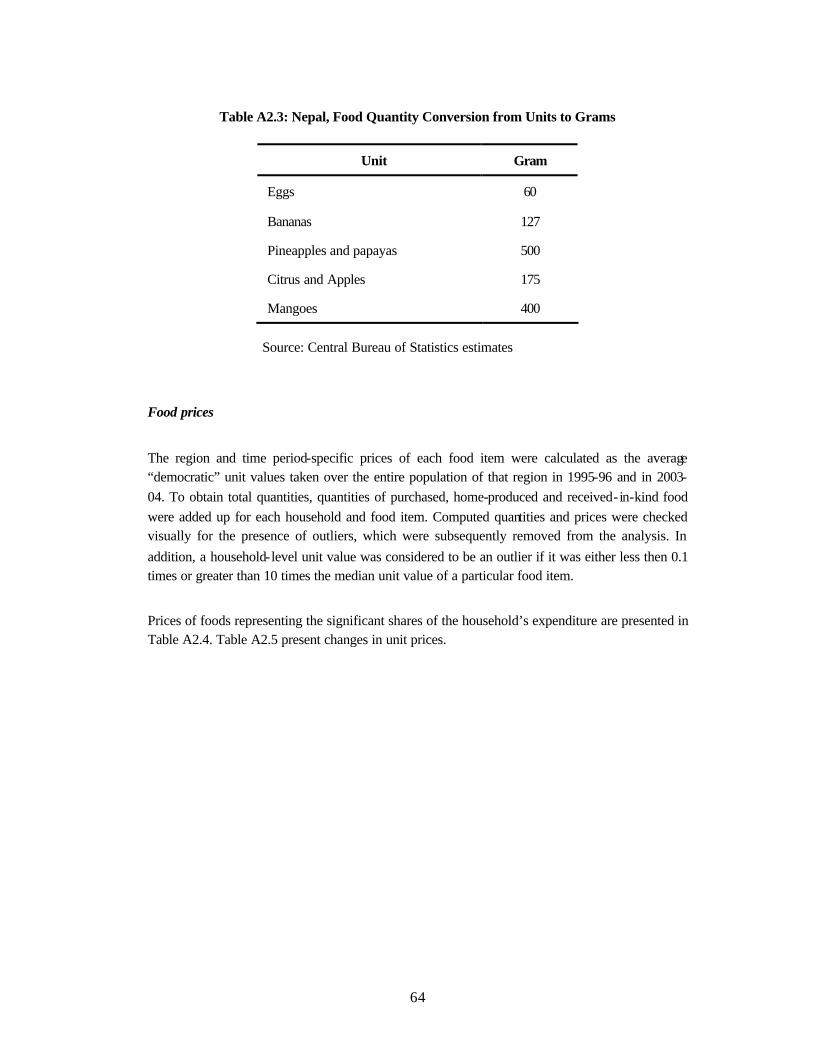
64
Table A2.3: Nepal, Food Quantity Conversion from Units to Grams
Unit Gram
Eggs 60
Bananas 127
Pineapples and papayas 500
Citrus and Apples 175
Mangoes 400
Source: Central Bureau of Statistics estimates
Food prices
The region and time period-specific prices of each food item were calculated as the average “democratic” unit values taken over the entire population of that region in 1995-96 and in 2003-04. To obtain total quantities, quantities of purchased, home-produced and received-in-kind food were added up for each household and food item. Computed quantities and prices were checked visually for the presence of outliers, which were subsequently removed from the analysis. In addition, a household-level unit value was considered to be an outlier if it was either less then 0.1 times or greater than 10 times the median unit value of a particular food item.
Prices of foods representing the significant shares of the household’s expenditure are presented in Table A2.4. Table A2.5 present changes in unit prices.
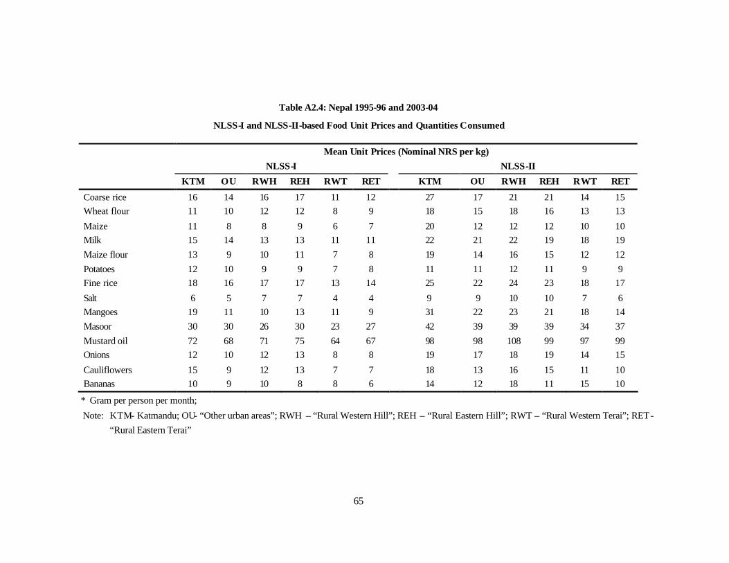
65
Table A2.4: Nepal 1995-96 and 2003-04
NLSS-I and NLSS-II-based Food Unit Prices and Quantities Consumed
Mean Unit Prices (Nominal NRS per kg) NLSS-I NLSS-II
KTM OU RWH REH RWT RET KTM OU RWH REH RWT RET
Coarse rice 16 14 16 17 11 12 27 17 21 21 14 15 Wheat flour 11 10 12 12 8 9 18 15 18 16 13 13
Maize 11 8 8 9 6 7 20 12 12 12 10 10 Milk 15 14 13 13 11 11 22 21 22 19 18 19 Maize flour 13 9 10 11 7 8 19 14 16 15 12 12 Potatoes 12 10 9 9 7 8 11 11 12 11 9 9 Fine rice 18 16 17 17 13 14 25 22 24 23 18 17
Salt 6 5 7 7 4 4 9 9 10 10 7 6 Mangoes 19 11 10 13 11 9 31 22 23 21 18 14 Masoor 30 30 26 30 23 27 42 39 39 39 34 37 Mustard oil 72 68 71 75 64 67 98 98 108 99 97 99 Onions 12 10 12 13 8 8 19 17 18 19 14 15
Cauliflowers 15 9 12 13 7 7 18 13 16 15 11 10 Bananas 10 9 10 8 8 6 14 12 18 11 15 10
* Gram per person per month;
Note: KTM- Katmandu; OU- “Other urban areas”; RWH – “Rural Western Hill”; REH – “Rural Eastern Hill”; RWT – “Rural Western Terai”; RET- “Rural Eastern Terai”
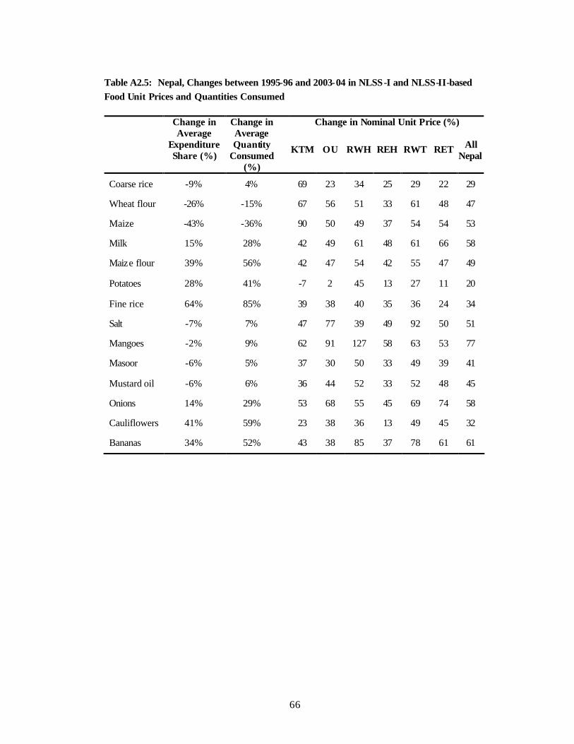
66
Table A2.5: Nepal, Changes between 1995-96 and 2003-04 in NLSS-I and NLSS-II-based Food Unit Prices and Quantities Consumed
Change in Nominal Unit Price (%) Change in Average
Expenditure Share (%)
Change in Average Quantity
Consumed (%)
KTM OU RWH REH RWT RET All Nepal
Coarse rice -9% 4% 69 23 34 25 29 22 29
Wheat flour -26% -15% 67 56 51 33 61 48 47
Maize -43% -36% 90 50 49 37 54 54 53
Milk 15% 28% 42 49 61 48 61 66 58
Maize flour 39% 56% 42 47 54 42 55 47 49
Potatoes 28% 41% -7 2 45 13 27 11 20
Fine rice 64% 85% 39 38 40 35 36 24 34
Salt -7% 7% 47 77 39 49 92 50 51
Mangoes -2% 9% 62 91 127 58 63 53 77
Masoor -6% 5% 37 30 50 33 49 39 41
Mustard oil -6% 6% 36 44 52 33 52 48 45
Onions 14% 29% 53 68 55 45 69 74 58
Cauliflowers 41% 59% 23 38 36 13 49 45 32
Bananas 34% 52% 43 38 85 37 78 61 61