SERIE DOCUMENTOS DE TRABAJO No. 99

Mayo 2011

POVERTY IMPACTS OF AGRICULTURAL POLICY ADJUSTMENTS IN

AN OPENING ECONOMY: THE CASE OF COLOMBIA

Ricardo Argüello C. Daniel Valderrama G. Sandra Acero W.

Poverty Impacts of Agricultural Policy Adjustments in an Opening Economy: the Case of Colombia

Ricardo Argüello C. Daniel Valderrama G.

Sandra Acero W.*

Abstract

We aim to contribute to the assessment of poverty impacts on the rural sector arising from agricultural policy adjustments in Colombia. For this we use an agriculture specialized static CGE model, jointly (sequentially) with a microsimulation model that allows for effective job relocation. Results indicate that the sectoral impact of the program implemented tends to be small and has considerable variability across crops. They also show that the highest impacts come from the irrigation and land improvements component of the program. Lastly, although it reduces poverty, poverty impacts are small and tend to concentrate in rural households toward the middle of the income distribution ladder.

JEL: Q18, I32, D58, C68 Keywords: Agricultural Policy, Colombia, AIS, Applied General Equilibrium, Rural

Poverty, Microsimulation

The findings, recommendations, interpretations and conclusions expressed in this paper are those of the authors and not necessarily reflect the view of the Department of Economics of the Universidad del Rosario. Associate Professor, Faculty of Economics, Universidad del Rosario. E-mail: arguello.ricardo@gmail.com. M.Sc. student and Young Researcher, Faculty of Economics, Universidad del Rosario. E-mail: danielvaldgon@gmail.com. * Independent agricultural expert.

2

1. Introduction On occasion of the negotiations for the establishment of a Free Trade Agreement between Colombia and the United States, the government agreed with representatives of agricultural producers to design and operate a program for compensating the losers from the agreement and for enhancing sectoral competiveness. A program for these purposes was launched in April 2007 and was given significant resources to operate. This policy package seems to reinforce a policy trend in Colombia toward increasing transfers to agricultural producers. In fact, a World Bank (2008) study shows that Colombia is the Latin American economy (among eight economies studied) that higher transfers makes per person engaged in agriculture in the region. With the resources deployed, it can be expected that the policy will have non-negligible effects on agricultural production and rural poverty reduction. As in other countries, Colombia shows high and persistent poverty rates in the rural sector and rural poverty, historically, has been higher than urban poverty. The aim of this research is to estimate the likely effects of this program at both the macro and micro levels. At the macro level we want to appraise the impact of this new agricultural policy on goods’ relative prices, production quantum, employment by sector, and real factor returns. At the micro level we want to assess induced changes in rural households income and on poverty incidence. For this, we use an integrated macro-micro approach in a top down fashion. First, we estimate macro changes using an agriculture specialized static computable general equilibrium model. Then, we use some results from the macro model to run a non-standard behavioral microsimulation model that allows for computing changes in rural households income and to measure their poverty status. The structure of the report is as follows. First, it provides a policy background for understanding the context in which policy changes take place; this is done in section 2. Second, it describes the way the policy package has been designed and is being implemented; a topic covered in section 3. Third, the research objective and the methodology are discussed, including a technical description of the main characteristics of the CGE model, as well as a general description of the microsimulation model are provided in section 4. A general description of the relevant characteristics of Colombian agriculture and rural poverty is the subject of section 5. Section 6 presents and discusses the results. Lastly, section 7 concludes. 2. Policy Background As other Latin American countries, Colombia has undergone a relatively ambitious process for opening up its economy during the last two decades. The average tariff has gone from 39% in 1990 (Bussolo and Lay, 2003) to 12% in 2005 -16.5% for agriculture (WTO, 2006). However, protection for the agricultural sector has remained relatively high, as tariffs for an important number of agricultural products are determined through the Andean Price Band

3

System (APBS) that ameliorates the impact of international prices. Even though it is meant as a price stabilization mechanism, the price band system confers an important degree of protection (Espinosa, 2005). The unweighted annual average tariff for the more than 150 agricultural tariff lines under the price band system in 2005 was 25%. Although decreasing in importance, the Colombian agricultural sector still plays a significant role in the economy. It represented 11% of GDP (World Bank, WDI database) and 19% of total exports –including agroindustry (Colombian Ministry of Trade, Industry and Tourism) in 2007, and 26% of employment in 2005 (Guterman, 2007). As part of this trade liberalization effort, Colombia finished negotiating a Free Trade Agreement (FTA) with the US in 2006 (modified by an amendment protocol in June 2007), finished negotiating an FTA with Canada in November 2008, and concluded negotiations for an Association Agreement with the European Union in the second quarter of 2010. Implementation of the FTA with the US is still pending, since the agreement has not yet been ratified by the US Congress (due mainly to human rights considerations). The agreement with Canada is in the process of ratification and the agreement with the EU was signed at the end of May 2010 and entered the ratification process. Once this set of FTAs gets implemented, about 64% of Colombian agricultural exports and 50% of agricultural imports will be liberalized. It turns out that adding up to these figures the share of agricultural trade that currently is covered by different FTAs’ provisions, about 83% of Colombian agricultural exports and 93% of agricultural imports will be “liberalized” in the near future.1 Bilateral trade with the United States is of topmost importance and is given a high priority in Colombian trade policy. United States’ shares in Colombian total imports and exports in 2005-7 were 27% and 38% respectively (Colombian Ministry of Trade, Industry and Tourism). The corresponding shares for agricultural trade were 39% and 35%. According to the USTR (2005), Colombia is the third largest destination for US agricultural exports in the Western Hemisphere –after Canada and Mexico. Partly for these reasons and partly due to the fact that the agricultural sector was expected to be one of the “losers” from bilateral trade liberalization with the US, in the midst of the negotiations for the FTA, the Colombian government agreed with representatives of the agricultural sector (basically, producers’ organizations) to design and implement a policy package for “compensating the losers from the agreement” (according to official statements for the press; El Tiempo, March 11, 2006). The announcement, made in March 2006, got into concretion in April 2007 with the approval by the Colombian Congress of AIS (Agriculture, Secured Income, by its acronym in Spanish). AIS is a policy package (a program) “aimed to protect the income of agricultural producers that may be affected by distortions arising from international markets and to enhance the competitiveness of the agricultural sector as a whole, given the internationalization of the economy.” (Colombian Congress, 2007; p. 1). AIS was assigned a total budget of around US$217 million for 2007 -the equivalent to about 35% of the 2007 total agricultural sector official budget, excluding debt servicing, or 48% of the Ministry of

1 Liberalized in the sense that trade is governed by FTAs’ rules; i.e. subject to a mix of tariff reductions, import quotas, tariff elimination, and in some cases, elimination of the APBS.

4

Agriculture’s budget, the organization in charge of its administration (Ministry of Agriculture, 2008). The program design was based on two main components. First, a set of direct support measures targeted toward protecting farmers income along a transition period, during which it is expected that sectoral competitiveness would be improved and a restructuring process for the agricultural sector would take place. No conditioning, in economic terms, is imposed on potential beneficiaries of these measures and the incentives are meant as selective and temporary. The government reserves the right to define “in an objective manner” the agricultural subsector that may benefit from them as well as their amount and the conditions that beneficiaries must fulfill. These measures cannot be granted beyond the first six years of operation of the program. The second component consists of a set of measures for enhancing competitiveness. Its objective is “to prepare the agricultural sector for the internationalization of the economy”, increase its productivity and launch restructuring processes along the whole sector. No less than 40% of total AIS resources must be devoted to finance this component. The central government assumes a commitment for supporting Departments (States) with low productivity and competitiveness indexes and to determine a regional distribution of AIS resources that is equitable. This policy comes on top of a policy trend toward increasing Nominal Rates of Assistance (NRA) for agriculture in Colombia. A recent report by the World Bank (2008) shows that Colombian agriculture has evolved from negative and (relatively) decreasing NRAs from 1965 to 1979 to positive and increasing NRAs between 1980 and 2004. A trend that is specially pronounced after the early 1990’s opening up of the Colombian economy, when NRAs went from 0.2% between 1985 and 1989 to 8.2% between 1990 and 1994, then to 13.2% between 1995 and 1999 and up to 25.9% between 2000 and 2004 (the end year of the study). The last figure puts Colombia as the economy granting the highest NRA for its agricultural sector among the eight Latin American countries under study, well above the 4.8% NRA found as a weighted average for the sampled countries and the 11.6% corresponding to Mexico (the economy with the second largest NRA), not to mention the negative 14.9% registered for Argentina (the lowest one). The same World Bank study shows that for a set of products representing around 52% of gross value of agricultural products at undistorted prices, the dispersion of NRAs across products (defined as the simple five-year average of the annual standard deviation around a weighted mean of NRAs across studied products for each year) reaches 46% (only below a staggering 132.8% for the Dominican Republic). This not only suggests concentration of policy assistance in some sectors, the study also shows that assistance is biased against exports. In fact, the NRA for exportables during 2000-2004 is 26% while that for importables is 46.2%, leading to a Trade Bias index of -0.13%. Furthermore, the set of products studied reduces to 11, 8 importables and 3 exportables, showing the high concentration of government assistance. In dollar (US) terms, the gross subsidy equivalent of assistance to farmers in Colombia amounted to 1,488 million during 1995-1999 and to

5

1,906 million during 2000-2004, yielding US$399 and US$515 per person engaged in agriculture (about a quarter of per capita GDP for the last period). With the inception of AIS this situation is likely to be more pronounced now, since there is an important overlap between the set of products selected for the World Bank study (the most prominent in terms of being targeted by sectoral policy) and those targeted by the program. It could be expected that, given the relative magnitude of government assistance to the agricultural sector, rural poverty should be decreasing in Colombia; however, this is not necessarily the case. The country has shown relatively high and persistent poverty. The poverty head count has remained in the range between 51% and 58% during the period 1996-2004 (Nuñez and Espinosa, 2005). As in other countries, poverty has been more widespread and intense in the rural sector. Along the period referred to, rural poverty has been 25 percentage points above urban poverty as an average. A recent report from the Mission for the Consistency of the Employment, Poverty, and Inequality Statistical Series, appointed by the Colombian National Statistical Department (DANE, 2009) reported national poverty incidence rates of 50.3% in 2005 and 46% in 2008 and rural poverty incidence rates of 67% and 65.2%, respectively (extreme rural poverty was estimated at 27.4% and 32.6%). Furthermore, evidence shows that rural poverty tends to concentrate among the population directly linked to the agricultural sector, especially small farm agriculture (CRECE, 2005). Therefore, it is reasonable to expect that trade liberalization will have an impact on rural poverty and that the same may be true with respect to policy measures implemented through AIS. 3. Implementation of AIS2 As mentioned, AIS was officially issued in April 2007 but the FTA with the US, that motivated its inception, has not yet entered in force (and it may be delayed for even more time, due to the priorities of the US government and the US Congress). To accommodate this fact, AIS gave priority to the Competitiveness Enhancement component (CEC). AIS’ 2007 budget was allocated as follows: 72% of total resources were allocated to the CEC, 26% to the Sectoral Direct Support component (SDSC), and the remaining 2% to the administration of the program. For 2008 the program was allocated around US$2713 (equivalent to 38%of the Ministry’s annual budget) of which 93.6% belong to the CEC, 5.2% to the SDSC, and 1.2% for the administration of the program. According to the law, the CEC has three main instruments: productivity incentives, subsidized credit, and marketing support. Productivity incentives are aimed at enhancing technical assistance, technology development and transfer, implementing good agricultural practices, associativeness, and land conversion, irrigation and drainage cofinancing. Subsidized credit is devoted to support productive restructuring, land conversion, productivity enhancement, and new investment for promoting agricultural modernization.

2 This section follows MADR (2008) 3 By law, from 2008 on the program should be allocated annually a minimum amount of COP$500.000 million, indexed by the Consumer Price Index.

6

Marketing support is targeted to the implementation of traceability systems, domestic absorption mechanisms, and other supplementary activities. During 2007, resources from CEC were channeled through a special credit line for production restructuring, enhancing agricultural investment, supporting irrigation and drainage projects, supporting research and technology transfer, enhancing investment through risk capital, and supporting sanitary measures for the livestock and poultry sectors. The special credit line for production restructuring offered the lowest interest rate available in the Colombian market (about 8% annual effective rate, 8 percentage points below the usual interest rate for small farmers and 12 percentage points below the usual rate for other farmers)4. It comprised about 31.3% of total AIS funds for the year, targeted for covering the credit subsidy. Table 1, provides details on the performance of the instrument. From there it can be appreciated that 0.21% of total projects were submitted by large farmers and accounted for more than 25% of funds, while 92% of projects were submitted by small farmers but they only accounted for 27% of disbursed funds. Also, credits to large farmers are predominantly devoted to acquisition of machinery for primary transformation of products, while in the case of small farmers are devoted to planting and maintenance of crops. In absolute terms, the majority of funds went to medium size farmers who devoted them to planting and maintenance of crops and land preparation.5 The average project value for large farmers is US$1.15 million, for medium size farmers is US$58,000, and for small farmers is US$2,785. Table 1. AIS Special Credit Line. Performance during 2007.

Producer/Credit line Projects (No.)

Projects share (%)

Value (US$ million)

Funds share (%)

Total 18,335 100 174.0* 100 Large farmers 39 0.21 45.0 25.84 Primary transformation 18 46.15 24.9 55.42** Planting and maintenance 8 20.51 7.1 15.88** Other 13 33.34 97.0 28.70**Medium size farmers 1,419 7.74 82 47.14 Planting and maintenance 655 46.16 36.6 44.59** Land preparation 232 16.35 16.9 20.59** Other 532 47.49 28.5 34.82**Small farmers 16,877 92.05 47 27.02 Planting and maintenance 14,685 87.01 41.9 88.98** Other 2,192 12.99 5.1 11.02**

*of these, US$68 million were assigned to pay for the subsidy of the interest rate **share on farmer type loans Source: MADR, 2008

4 The subsidy rate varies from year to year as new rules are put in place annually. For 2008 the subsidy rate decreased. 5 Small farmers are defined as those having family assets below US$30,000, with at least 75% of them invested in the agricultural sector and whose income stems from agricultural activities in at least two thirds.

7

The policy instrument used for enhancing agricultural investment, called Incentive for Rural Capitalization (IRC), is broader than AIS. The instrument existed prior to AIS but with the implementation of the latter it was amplified; that is, some of AIS resources are channeled under IRC, and IRC under AIS finances an slightly broader set of activities. IRC works as an incentive toward enhancing new rural investment by means of a credit line (at market interest rates) and limited credit forgiveness. Small producers are given 40% forgiveness on the value of the credit devoted to activities included in a list. Medium size and large farmers are given 20% forgiveness subject to some exceptions (related to some activities). In the case of construction, enlargement or rehabilitation of large irrigation projects, forgiveness is at the level of 40%, regardless of farmer size, and there are no limits in the amount of the incentive. The list of eligible activities includes land preparation and water management; productive infrastructure; biotechnology development and application; machinery and equipment for agricultural production; livestock and aquaculture equipment; low technology fishing; primary transformation of agricultural goods; planting, maintenance, and renewal of perennial crops; acquisition of pure breed bovine livestock; implementation of integrated livestock and forestry projects; and investment in generic agricultural inputs. IRC projects under AIS reached a total of 23,005 during 2007 with a total value of more than US$560 million for which US$332 million in credits were applied for and about US$29 million were accounted for as forgiveness. Medium size and large farmers represented 32.5% of total projects and 61.1% of IRC applied for (the basis under which credit forgiveness is calculated). Small farmers represented the remaining 67.5% of projects and 38.9% of IRC applied for. In sum, 44% of funds allocated to debt forgiveness went to medium size and large farmers and the rest to small farmers. The average size of the project for medium size and large farmers was US$60,109 and of US$7,174 for small farmers. During 2007, support for irrigation and drainage projects amounted to US$18.2 million, support for research and technology transfer to US$8.1 million, a risk capital fund was created with an AIS disbursement of US$24.4 million, and US$5.8 million were allocated for supporting sanitary measures for the livestock and poultry sectors. With respect to the SDSC, the whole amount of resources assigned to the component in 2007 was targeted to the cereals and rice sectors; US$40.9 million for cereals (sorghum, soybeans, beans, barley, and wheat) and US$15.1 million for rice. Resources assigned to cereals were channeled through the special credit line, 47.6%, and the IRC, 53.4%. Similarly, resources devoted to rice were disbursed through the special credit line, 40%, and the IRC, 60%. Given the nature of the component, conditions for the IRC differ from the general ones. Debt forgiveness for small farmers is, again, 40% but for medium size and large farmers it is increased to 30%. Also the maximum credit is extended to a ceiling equivalent to 1,500 legal minimum monthly wages (about US$353,000). 4. Research Objective and Methodology Our main research objectives are to estimate the likely sectoral impact of the newly introduced agricultural policies, as well as its likely effect on rural poverty. In particular, to assess the potential impact of the main components of AIS on agricultural goods’ relative

8

prices, production quantum, and real factor returns and the way they impinge upon rural households income generation. Given the strong targeting of AIS we also aim at identifying the main winners and losers, in terms of goods and households, that the program will generate within the rural sector. For this, we integrate an agriculture specialized static CGE model and a microsimulation model that allows effective labor relocation within occupational groups for the agricultural sector. The CGE is used for simulating the impact on relative prices and macro variables of sectoral policies. Changes in macro variables (wages, employment by agricultural sub-sector, etc.) are fed into the microsimulation model. The latter allows for a rich simulation of changes in rural households income, providing a sound basis for assessing the poverty effects induced by sectoral policies. The approach we follow here is top-down, so there are no interactions between the two models in a loop. There are a number of advantages in using microsimulation models linked to macro models (Savard, 2003). First, we can accommodate a large number of households without the difficulties inherent to incorporating them directly into the CGE model. Second, discrete-choice or integer behavior can be incorporated much more easily into the household model than into the CGE model, and they may be important for modeling the rural sector. While there is no need to assure consistency between household data used in the microsimulation model and SAM data when there is looping, we need to assure it from the beginning. The reason is that without looping there is no guarantee that results from the two models will converge. Using a top-down approach without feedback, as we do here, there is no convergence in any strict sense. Therefore, having consistency between the macro and the micro data assures us that changes in “macro” variables (prices and quantities mainly), in the aggregate, have the “right” impact on households. Simulation of sectoral policy changes uses the 2008’s allocation of AIS’ resources to the different policy instruments. 4.1 The CGE Model The CGE model is based upon the PEP Standard CGE model (single country, static; PEP-1-1). It has a neoclassical structure with equations that describe producers’ production and input decisions, households’ behavior, government demands, import demands, market clearing conditions for commodities and factor markets, and numerous macroeconomic variables and price indices. Demand and supply equations for private-sector agents are derived from the solutions to optimization problems, in which it is assumed that agents are price-takers and markets competitive. The external sector is modeled as a single region and a “mild” version of the small country assumption is used.6 A thorough documentation of the model is found in Decaluwé et al (2009). The adjustments made to the PEP-1-1 model mainly refer to the treatment of the agricultural sector. They draw on several sources and concentrate around the treatment of supply of land

6 In the sense that local producers can increase their share in international markets as long as they can offer a price that is advantageous with respect to the world price (and subject to a price elasticity of export demand).

servdesc 4.1.1 The assuSectat th(CEcomcapigood

Figu Whithis due Theschansectoagricvarie Withthe

vices and thacribed below

1 Agricult

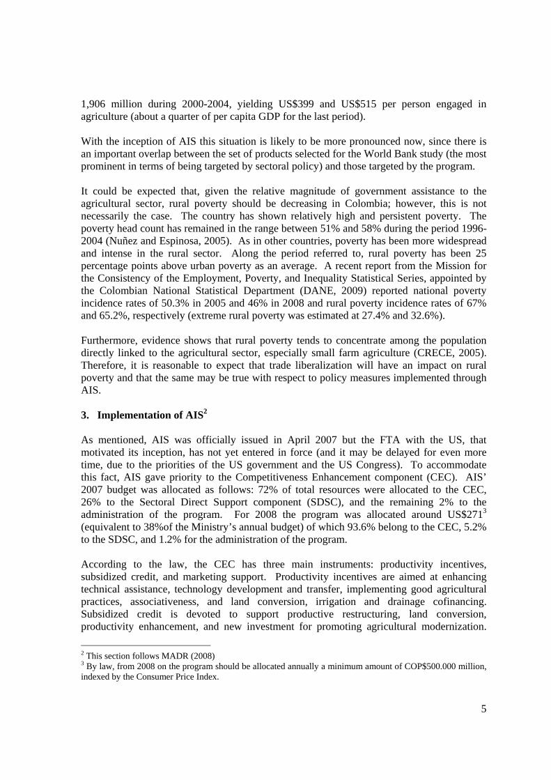
structure oumed to opetoral outputhe second leS) manner,

mbination ofital types. Lds and servi

ure 1. Struc

ile adequaterepresentatito the fact se features nges impingor is modificulture is reties of live

h this definitop, value

at of agriculw.

tural Activit

of productioerate in a cot uses valueevel, sector, a composf different laLastly, intermices used in

cture of prod

e for manufion does nothat it doesare also i

ge upon the ied as illustrrestricted toestock activi

ition in placadded and

ltural produ

ties

on in PEP-1ompetitive m added and

ral value adsite of laboabor types, mediate conthe product

duction in P

facturing prot fit very w not considimportant fbehavior o

rated belowo productioities, dairy p

ce, agricultud a compos

uction. The

-1 is illustrmarket and intermediat

dded combinor and capiand compo

nsumption istion process

EP-1-1 (tak

roduction orwell in an ag

er several dfor capturinf the sector

w. It is impoon of seasonproduction,

ural activitiesite interme

key feature

rated in Figto maximiz

te consumpnes, in a Coital. Comp

osite capital s a fixed pros.

ken from De

r as a genergriculture spdesirable feang the extenr. Thereforeortant to notnal and pemeat produ

es are modeediate good

es of the mo

gure 1. As ze profits su

ption in fixeonstant Elasposite laboa CES com

oportions ag

ecaluwe et a

ral represenpecialized matures of agnt to whiche, productiotice though rennial cropction, forest

led as illustd are used

del in this r

mentioned,ubject to te

ed proportiosticity of Sur, in turn

mbination ofggregate of

al (2009).

ntation of prmodel, as neegricultural prh agricultur

on for the agthat our deps, leavingtry and fishe

trated in Figin fixed pr

9

respect are

firms are echnology. ons, while, ubstitution is a CES f different individual

roduction, eded here, roduction. ral policy gricultural finition of aside all eries.

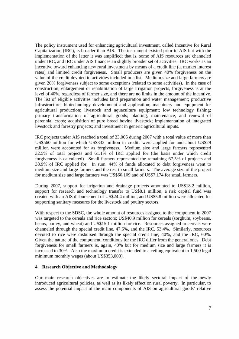
gure 2. At roportions

10

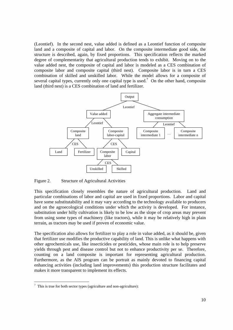
(Leontief). In the second nest, value added is defined as a Leontief function of composite land and a composite of capital and labor. On the composite intermediate good side, the structure is described, again, by fixed proportions. This specification reflects the marked degree of complementarity that agricultural production tends to exhibit. Moving on to the value added nest, the composite of capital and labor is modeled as a CES combination of composite labor and composite capital (third nest). Composite labor is in turn a CES combination of skilled and unskilled labor. While the model allows for a composite of several capital types, currently only one capital type is used.7 On the other hand, composite land (third nest) is a CES combination of land and fertilizer. Figure 2. Structure of Agricultural Activities This specification closely resembles the nature of agricultural production. Land and particular combinations of labor and capital are used in fixed proportions. Labor and capital have some substitutability and it may vary according to the technology available to producers and on the agroecological conditions under which the activity is developed. For instance, substitution under hilly cultivation is likely to be low as the slope of crop areas may prevent from using some types of machinery (like tractors), while it may be relatively high in plain terrain, as tractors may be used if proven of economic value. The specification also allows for fertilizer to play a role in value added, as it should be, given that fertilizer use modifies the productive capability of land. This is unlike what happens with other agrochemicals use, like insecticides or pesticides, whose main role is to help preserve yields through pest and disease control but not to enhance productivity per se. Therefore, counting on a land composite is important for representing agricultural production. Furthermore, as the AIS program can be portrait as mainly devoted to financing capital enhancing activities (including land improvements) this production structure facilitates and makes it more transparent to implement its effects. 7 This is true for both sector types (agriculture and non-agriculture):

CESCES

CES

Leontief Leontief

…

Output

Value added Aggregate intermediate consumption

Composite land

Composite labor-capital

Land Fertilizer Capital Composite labor

Composite intermediate 1

Composite intermediate n

Skilled Unskilled

Leontief

11

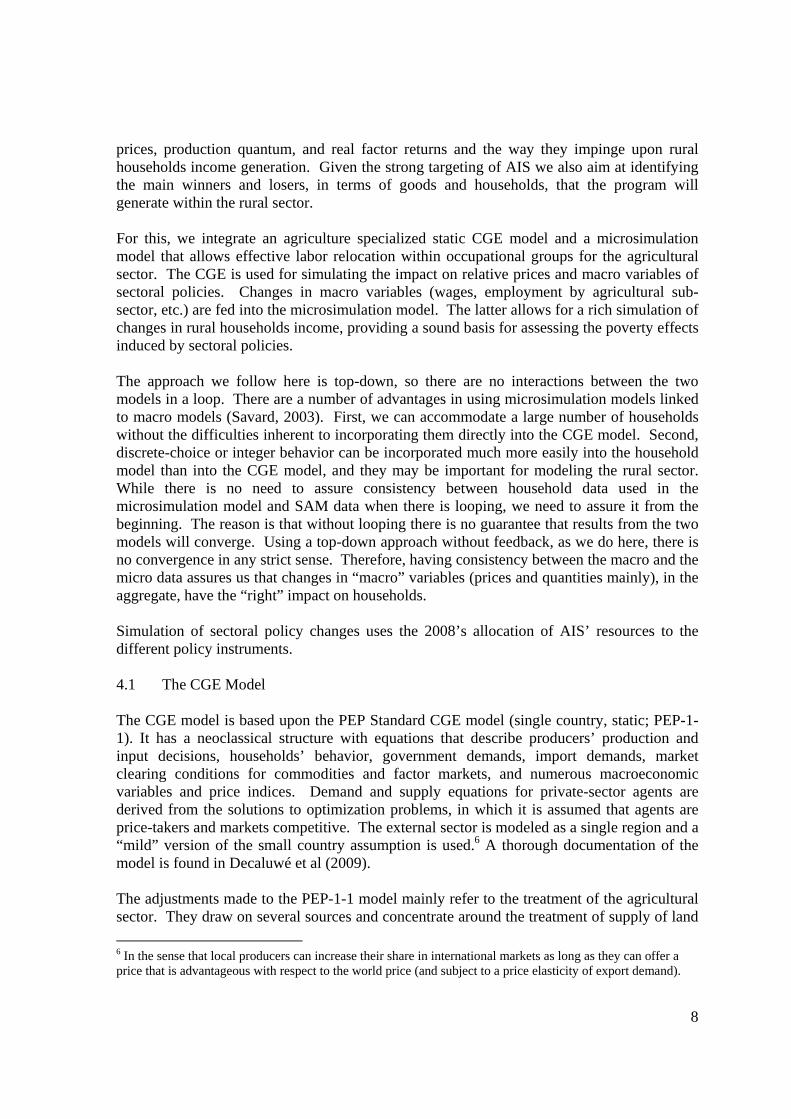
The model considers no special crops-livestock interactions (i.e., use of crops as a source of animal feed) beyond the usual input-output relationship. As Colombian cattle and milk production activities are basically extensive in nature and, therefore, based on pastures (either planted or not) this is a reasonable simplification. The way this production structure is implemented in the model is fully described in the Appendix. 4.1.2 Treatment of Land Agricultural land is assumed homogeneous in the model and only land for agricultural use is considered (no land services for livestock, forestry, and industrial use are taken into account). This means that crops compete for land services with no regard for the agroecological conditions that they require. However, land services are rendered to each crop type with certain restrictions. This feature, responds to two considerations. First, it approximates the fact that land is not in actuality homogeneous. Land availability is tied to climate and other characteristics that suite some crops but not others and, as a consequence, it cannot be freely “mobile” across crops. Second, agricultural land use is conditioned upon certain economic constraints. In particular, land use may depend on the easiness with which land can be allocated to different crop types, according to characteristics such as the way cash flows produced or required by the activity behave, or to the size of initial investments. Therefore, in spite of being considered homogeneous, land allocation is “sluggish” in the model. Land allocation is done according to the degree of “easiness of entry” into a particular activity. Activities for which it is required to make sizeable investments in land preparation or for which the maturing period is large, are deemed to experience lower propensities to be switched to from other uses. Hence, land allocation is modeled as a nested Constant Elasticity of Transformation (CET) structure (Figure 3). The supply of land services at the top is divided among perennial and seasonal crops (first nest with an elasticity given by 1). This is a decision usually associated to the need for relatively lumpy investments and cash flow constraints, given that perennials take some time to begin producing. Then, in the second nest land is allocated to particular crops (both perennial and seasonal with elasticities given by 2 and 3, respectively). At this level, land allocation decisions differ according to the type of crop. Land allocation within seasonal crops is the most flexible given that investments required to switch from one crop to the other are relatively low. In contrast, land allocation between perennials is less easy as switching from one crop to the other entails incurring in higher costs. The following relationship holds for the three elasticities: 1< 2< 3. This structure is akin to that used in models that portrait land as differentiated in Agro-Ecological Zones (AEZs), like in Darwin et al (1995), Hertel et al (2008), and as reviewed in Hertel et al (2007). Imperfect land mobility between land uses, modeled with a CET function as illustrated above, yields a land supply frontier rather than a production possibilities frontier (Baltzer and Kloverpris, 2008). That is, the land supply frontier, determined by the CET, assigns land services between crops according to changes in land rents associated to each crop. As long as land rents differ across crops, equilibrium can be reached only if land supply is aggregated

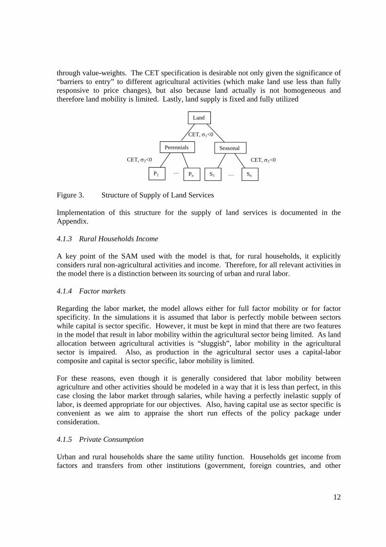
12

through value-weights. The CET specification is desirable not only given the significance of “barriers to entry” to different agricultural activities (which make land use less than fully responsive to price changes), but also because land actually is not homogeneous and therefore land mobility is limited. Lastly, land supply is fixed and fully utilized Figure 3. Structure of Supply of Land Services Implementation of this structure for the supply of land services is documented in the Appendix. 4.1.3 Rural Households Income A key point of the SAM used with the model is that, for rural households, it explicitly considers rural non-agricultural activities and income. Therefore, for all relevant activities in the model there is a distinction between its sourcing of urban and rural labor. 4.1.4 Factor markets Regarding the labor market, the model allows either for full factor mobility or for factor specificity. In the simulations it is assumed that labor is perfectly mobile between sectors while capital is sector specific. However, it must be kept in mind that there are two features in the model that result in labor mobility within the agricultural sector being limited. As land allocation between agricultural activities is “sluggish”, labor mobility in the agricultural sector is impaired. Also, as production in the agricultural sector uses a capital-labor composite and capital is sector specific, labor mobility is limited. For these reasons, even though it is generally considered that labor mobility between agriculture and other activities should be modeled in a way that it is less than perfect, in this case closing the labor market through salaries, while having a perfectly inelastic supply of labor, is deemed appropriate for our objectives. Also, having capital use as sector specific is convenient as we aim to appraise the short run effects of the policy package under consideration. 4.1.5 Private Consumption Urban and rural households share the same utility function. Households get income from factors and transfers from other institutions (government, foreign countries, and other

CET, 1<0

CET, <0 CET, <0

Land

Perennials Seasonal

P1 Pn S1 Sn … …

13

households). Consumption income is the residual after paying taxes, savings, and transfers to other institutions, and is spent according to Linear Expenditure System (LES) demand functions derived from a Stone-Geary utility function. We consider no self-consumption of agricultural goods produced by rural households. 4.1.6 Other Characteristics of the Model Firms may receive factor income and transfers from other institutions. This income may be allocated between direct taxes, savings, and transfers to other institutions. The government collects taxes and gets transfers from other institutions and expends this income on purchasing commodities, and transfers to other institutions. Government consumption is endogenous while transfers to domestic institutions are CPI-indexed, and savings is a residual. Foreign savings is the difference between foreign currency spending and receipts. Regarding commodity markets, aggregate domestic output may be sold in the domestic market or exported and the allocation is done through a CET function. Activity-specific commodity prices clear the implicit market for each disaggregated commodity. As mentioned before, a mild version of the small country assumption is used with respect to international trade; therefore, domestic exporters can increase their share in international markets under appropriate circumstances. On the other side, unlimited quantities of imports can be channeled from abroad at international prices. Domestic demand comes from households and government consumption, investment, intermediate inputs, and transaction inputs. Aggregate imported commodities and domestic output are imperfect substitutes in demand (using a CES function). As for the tax system, income taxes are defined as a linear function of total income allowing use of marginal effective tax rates. The rest of taxes are at fixed ad valorem rates, as are tariff rates. 4.1.7 Policy modeling As mentioned before, we aim to simulate the impact of some of AIS’ policy instruments. Independently of the program component (CEC or SDSC), the operational structure of AIS determines the way the impact of the policy instrument should be modeled. AIS is mainly based on the following set of policy instruments (the description includes only agricultural activities).

a. Subsidized credit for working capital for planting of seasonal crops and maintenance of any crop type. Eligible items include land preparation, seeds, fertilizer, technical assistance, phitosanitary control, irrigation, roads, support infrastructure; and land leasing. Financing is done through the Special Credit Line (SCL) and covers up to 100% of the direct cost of the project for small farmers, and up to 80% of total direct costs for medium and big farmers. The SCL has a general component, in the framework of the CEC, and a sectoral component, in the framework of the SDSC. Until recently, interest rates were different for both components and across farmers. Currently, interest rates have been unified at the

14

market passive interest rate (MPIR)8 for small farmers, and the MPIR plus 2 percentage points for medium size and big farmers.9 The commercial banks’ interest rate for agricultural activities outside AIS is the MPIR plus 6 percentage points in the case of small farmers and the MPIR plus 10 percentage points in the case of medium size and big farmers. Given that most agricultural projects financed through this policy instrument cover the whole or a sizeable part of the production cycle, including the majority of the production and harvesting activities, and that most of financing for infrastructure is done through other means, the instrument is modeled as a direct production subsidy, as specified below. = 1 + (1 − ) where: = = = = ℎ A full description of the way this subsidy is modeled is provided in the Appendix.

b. Subsidized credit for infrastructure for storage and marketing. Eligible items include investment costs in infrastructure, purchases of new machinery and equipment, and specialized transport. There are two main sources of financing in this case: the SCL, under the conditions above mentioned, and the IRC. Projects can be financed only through one of these sources. As mentioned before, credits under the IRC provide for partial credit forgiveness: 40% of the total project value for small farmers, 30% for medium size farmers, and 20% for big farmers. Given the nature of the instrument, its effect is modeled as a reduction in the cost of trade and transport services (margins) incurred by agricultural activities, as illustrated in the following. , = , − , , = , − , , = , − , where: , = ’ , = ’

8 The market passive interest rate is the interest rate paid by banks to depositors on the moneys put in publicly available instruments (certificates of deposit) with a maturing period of at most one year. 9 These interest rate levels were established in 2010. The interest rate before this change was the MPIR minus 2 percentage points, irrespective of the type of beneficiary, for the CEC and even more favorable under the SDSC component. Also, it was established that 50% of total program resources should be allocated to small farmers, 30% to medium size farmers, and the remaining 20% to big farmers. The current interest rate entails a subsidy in the order of around 7 percentage points (annual effective) vis a vis the market interest rate.

15

, = ’ , = , = , = = , ∈ = , ∈ = , ∈ A full description of the way this subsidy is modeled is provided in the Appendix.

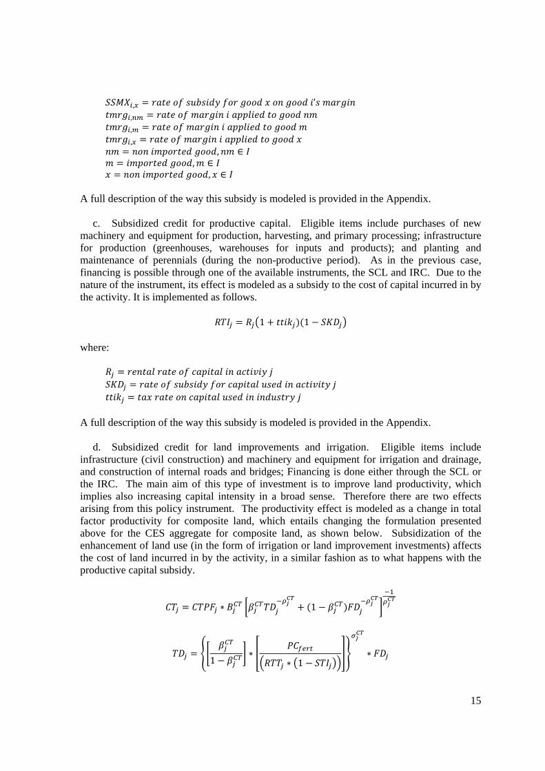
c. Subsidized credit for productive capital. Eligible items include purchases of new machinery and equipment for production, harvesting, and primary processing; infrastructure for production (greenhouses, warehouses for inputs and products); and planting and maintenance of perennials (during the non-productive period). As in the previous case, financing is possible through one of the available instruments, the SCL and IRC. Due to the nature of the instrument, its effect is modeled as a subsidy to the cost of capital incurred in by the activity. It is implemented as follows. = 1 + )(1 − where: = = = A full description of the way this subsidy is modeled is provided in the Appendix.

d. Subsidized credit for land improvements and irrigation. Eligible items include infrastructure (civil construction) and machinery and equipment for irrigation and drainage, and construction of internal roads and bridges; Financing is done either through the SCL or the IRC. The main aim of this type of investment is to improve land productivity, which implies also increasing capital intensity in a broad sense. Therefore there are two effects arising from this policy instrument. The productivity effect is modeled as a change in total factor productivity for composite land, which entails changing the formulation presented above for the CES aggregate for composite land, as shown below. Subsidization of the enhancement of land use (in the form of irrigation or land improvement investments) affects the cost of land incurred in by the activity, in a similar fashion as to what happens with the productive capital subsidy. = ∗ + (1 − )

= 1 − ∗ ∗ 1 − ∗

16

where: = = = = = . = = ( − ) = ℎ ( − ) = ( − ); −1 < < ∞

A full description of the way this subsidy is modeled is provided in the Appendix.

e. Financing of the program’s subsidies. As there is need to finance governmental expending for subsidizing agricultural activities as depicted above, an increase in direct taxes is employed for this end. Both, households and firms taxes are raised in proportion in order to increase government income as required by implementation of the policy package. This is done as follows: = ∗ ℎ0 + ℎ1 + ∗ = ∗ 0 + 1 + ∗ where: = = = ℎℎ ℎ = = ℎℎ ℎ = ℎ0 = ( ℎℎ ℎ ) ℎ1 = ℎℎ ℎ 0 = ( ) 1 = = A full description of the way the mechanism is modeled is provided in the Appendix. 4.2 The Microsimulation Model We use a non standard behavioral approach for the microsimulation model. It is non standard in that we do not seek to mimic household behavior in terms of labor participation or labor choice for household members. Instead, we combine parametric and nonparametric

17

approaches in and ad hoc fashion that suits well the structure of data on which we construct the microsimulation model, as explained below. Based on the Colombian 2008 LSMS we construct a household database that is consistent with macro data (the SAM on which the CGE runs) in terms of the aggregate wage bill, capital income, land income, and transfers. The database keeps all relevant household and individual´s information such as number of adult equivalents, occupational status, gender, relationship to household head, employment status, age, type of activity, land holdings, income (from different sources), and sample weights. Wage equations are estimated through a two-stage Heckman procedure for economically active (and employed) people belonging to the four labor types considered in the macro model. Estimated parameters are kept in the database and residuals from each individual’s estimation are also stored. The stored parameters and residuals are used to update wages for each individual, using percentages changes coming from the CGE model simulation. Individuals’ income, explained through the wage equation, is increased as indicated by the CGE results and then residuals are added so as to (approximately) preserve unexplained income and income variation among individuals. The specification of the labor market in the CGE model uses wages as the market clearing mechanism and, therefore, there is no unemployment. In spite of this, and considering that our main interest is in income changes at the rural household level, as they relate to changes in agricultural activities, we exploit a feature of agricultural production to mimic changes in employment. Being Colombia a tropical country, crops can be classified according to regions where they can be cultivated. This gives us a partition in three regions defined according to their altitude above sea level: hot weather, mild weather, and cold weather areas. Changes in employment for each agricultural sector can then be assigned to each of these regions. For crops that are suitable for more than one region, employment changes are split between regions according to the shares of each region in that crop’s planted area. In general, for a worker moving from one region to another is tantamount of having to migrate. We assume that workers (and households) remain in their locations and that it is employment that “moves” from one region to another, as crops belonging to a region increase or decrease their demand for labor types. We have, therefore, labor markets for each labor type in each region and it is within these “segmented” markets that we can mimic employment level changes. We use information from the household survey to assign households to the three regions, so we also have this characteristic in the database. Given the above, we can draw unemployed workers to get into the labor market when their labor type has an increase in employment level in a region, or expel workers when there is a decrease. For this we build a queue based on the probability that an individual, whether employed or unemployed, gets fired or gets a job. We obtain these probabilities by means of a probit model.

18

To get around the problem that arises when changes in employment yield non-integer values, we borrow from Ferreira-Filho and Horridge (2004). They use a procedure that they call the “quantum weights method”. The basic idea is simple. A variable, JobScore, is created for each person in the database and is set to 1 if she is employed. Then, when there are changes in employment, this variable is used to split the record and with it the sample weight in such a way that the non-integer figure can be accommodated. The procedure entails splitting the household into two households in such a way so as to replicate the change in the simulated JobScore. This is accommodated by dividing the sample household weight to yield the desired result (the simulated value for JobScore). The two households share the same characteristics, but one has, say, one working adult with a given sample weight (resulting from the division above) and the other an unemployed adult with another sample weight (the complement of the former). In general, a new record is created for each worker with JobScore < 1 and for each unemployed within a labor type and region, for which demand increases. The procedure is followed only for the (infra) marginal worker. Individuals that move from unemployment into employment, get a wage level determined according to the parameters of the wage equation, taking into account the wage change coming from the CGE model. To this income we add an unexplained income calculated from a random draw based on the residuals from the wage equation (as applied to employed workers). As employment changes apply only to agriculture related jobs, it is assumed that changes in employment arising from the rest of the economy are allocated to individuals based on their probability of being fired, irrespective of whether the household they belong to has members working in agricultural activities and irrespective of the region they belong to. Other household income, in particular income from land holdings and capital is updated on the basis of rent changes for these two factors. For poverty calculations, the poverty line is also updated according to changes in the consumer price index. 4.3 Linking the Two Models Consistency between the macro (SAM) and micro (LSMS) data is assured at the beginning, by appropriately adjusting individuals and households’ income, taking sample weights into consideration, to the corresponding macro aggregates. The main features for linking the two models have been presented above. The micro model is fed with percentage changes in employment by labor type and region (weather-based, as described above), providing the basis for the job realocation process performed with it. Also, as changes in labor demand in the agricultural sector have its counterpart in changes in employment in the rest of the economy, employment changes for the latter are also transmitted from the macro model. On the other hand, percentage price changes are fed into the microsimulation model. These refer to wages for each labor type, capital rent, land rent, and the consumer price index, to be used as explained above.

19

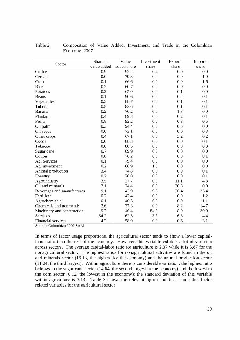
4.4 Data The CGE model uses a 2007 SAM with 31 activities and 31 commodities. 22 activities and commodities belong to the agricultural sector, 10 are seasonal crops, 8 are perennial crops, and the remaining four are perennials that are not productive yet (investment), livestock and poultry, forestry, and agricultural services. Among the non-agricultural sectors, there are two services sectors (services in general and financial services) and two sectors providing agricultural inputs (fertilizers and other agrochemicals). There are three production factors: land, labor, and capital. Land is used only by crops, so livestock and poultry, forestry, and agricultural services, only use labor and capital. Labor is split into four categories, rural unskilled, rural skilled, urban unskilled, and urban skilled, and there is only one type of capital. Households are disaggregated into rural and urban and each type is, in turn, split in income quintiles. The micro SAM has been constructed based upon the 2006-7 National Income and Expenditures Household Survey and the 2008 National LSMS. The latter is the input for the microsimulation model. It contains data on more than 13,000 households and is statistically significant at the urban/rural levels as well as at the level of nine broad regions. 5. Stylized facts about the Colombian agricultural sector and rural poverty For easiness of interpretation of the results it is useful to provide a general description of the Colombian economy with emphasis on the agricultural sector. Table 2 shows some of the basic macro statistics at the sectoral level. From there it can appreciated that the services sector is by far the largest contributor to total value added (first column), followed by Machinery and construction, and Beverages and manufactures. The agricultural sector, including animals and forestry, accounts for a bit more than nine percent of total value added and for 5.7% if only crops are included. The share of value added in total sectoral value (second column) is higher for the agricultural sector as compared to other sectors in the economy. As an average, value added accounts for around 80% of total sectoral value in the agricultural sector, while it only reaches 49% for the rest of the economy. The largest value added shares are found in the oil palm, fruits, coffee, and beans sectors. As could be expected, machinery and construction make up for the bulk of investment, followed at distance by beverages and manufactures, and services. With respect to international trade, the majority of export value (almost 70%) is concentrated in three sectors: oil and minerals, beverages and manufacturing, and agroindustry (mainly green coffee). If exports of chemicals and nonmetals and machinery and construction are added, the five sectors account for almost 85% of total exports. On the import side, Beverages and manufactures, machinery and construction, and chemicals and nonmetals, account for around 80% of total imports. As follows from the data, the share of the agricultural sector in international trade is low, 6.2% of total exports and 4.1% of total imports. The highest participation of an agricultural sector is found for exports of other crops (3.2%), a result due to fresh cut flower exports.

20

Table 2. Composition of Value Added, Investment, and Trade in the Colombian Economy, 2007

Sector Share in

value addedValue

added share Investment

share Exports

share Imports share

Coffee 0.9 92.2 0.4 0.0 0.0 Cereals 0.0 79.3 0.0 0.0 1.0 Corn 0.1 66.6 0.0 0.0 1.6 Rice 0.2 60.7 0.0 0.0 0.0 Potatoes 0.2 65.0 0.0 0.1 0.0 Beans 0.1 90.6 0.0 0.2 0.1 Vegetables 0.3 88.7 0.0 0.1 0.1 Tubers 0.5 83.6 0.0 0.1 0.1 Banana 0.2 70.2 0.0 1.5 0.0 Plantain 0.4 89.3 0.0 0.2 0.1 Fruits 0.8 92.2 0.0 0.3 0.5 Oil palm 0.3 94.4 0.0 0.5 0.0 Oil seeds 0.0 73.1 0.0 0.0 0.3 Other crops 0.4 67.1 0.0 3.2 0.2 Cocoa 0.0 88.3 0.0 0.0 0.1 Tobacco 0.0 88.5 0.0 0.0 0.0 Sugar cane 0.7 89.9 0.0 0.0 0.0 Cotton 0.0 76.2 0.0 0.0 0.1 Ag. Services 0.1 79.4 0.0 0.0 0.0 Ag. investment 0.2 66.9 1.5 0.0 0.0 Animal production 3.4 74.8 0.5 0.9 0.1 Forestry 0.2 76.0 0.0 0.0 0.1 Agroindustry 3.5 27.7 0.0 11.1 4.8 Oil and minerals 7.1 74.4 0.0 30.8 0.9 Beverages and manufactures 9.1 43.9 9.3 26.4 35.4 Fertilizer 0.2 42.4 0.0 0.9 1.2 Agrochemicals 0.1 46.3 0.0 0.0 1.1 Chemicals and nonmetals 2.6 37.3 0.0 8.2 14.7 Machinery and construction 9.7 46.4 84.9 8.0 30.0 Services 54.2 62.5 3.3 6.8 4.4 Financial services 4.2 58.9 0.0 0.6 3.1 Source: Colombian 2007 SAM In terms of factor usage proportions, the agricultural sector tends to show a lower capital-labor ratio than the rest of the economy. However, this variable exhibits a lot of variation across sectors. The average capital-labor ratio for agriculture is 2.37 while it is 3.87 for the nonagricultural sector. The highest ratios for nonagricultural activities are found in the oil and minerals sector (16.13, the highest for the economy) and the animal production sector (11.04, the third largest). Within agriculture there is considerable variation: the highest ratio belongs to the sugar cane sector (14.64, the second largest in the economy) and the lowest to the corn sector (0.12, the lowest in the economy); the standard deviation of this variable within agriculture is 3.13. Table 3 shows the relevant figures for these and other factor related variables for the agricultural sector.

21

Table 3. Factor Intensity Use Across Agricultural Activities in Colombia, 2007

Sector K/L ratio T/L ratio K/T ratio Coffee 0.74 0.09 7.93 Cereals 1.90 0.44 4.36 Corn 0.12 0.36 0.33 Rice 3.16 1.12 2.82 Potatoes 0.99 0.18 5.54 Beans 4.07 0.19 21.98 Vegetables 3.36 0.21 16.03 Tubers 2.78 0.32 8.64 Banana 1.37 0.09 16.03 Plantain 1.19 0.34 3.45 Fruits 2.76 0.15 19.00 Oil palm 2.88 0.30 9.73 Oil seeds 3.06 2.03 1.51 Other crops 0.20 0.04 5.50 Cocoa 0.58 0.28 2.11 Tobacco 1.26 0.11 11.39 Sugar cane 14.64 4.63 3.16 Cotton 0.46 0.18 2.62 Ag. investment 0.29 0.03 9.44

Source: Colombian 2007 SAM Land-labor ratios (second column in Table 3), tend to be low in Colombian agriculture. The highest ratio is found in the case of the sugar cane sector, while the lowest pertain to the agricultural investment sector.10 The average land-labor ratio is 0.58 and its standard deviation is 1.09. Lastly, capital-land ratios (third column) also show high variability within agriculture. The largest ratio shows up for the beans sector, followed by the fruits, and banana sectors. The lowest ratio belong to the corn sector, followed by the oil seeds sector, and the cocoa sector. The average ratio for agriculture is 8 and its standard deviation is 6.34. As for shares in factor use, the agricultural sector is relatively weak, as can be inferred from its participation in value added. Agriculture accounts for 5.3% of total labor use and 4.5% of total capital use. Coffee has the highest share in labor demand, while several sectors have shares less than 0.1%. The highest shares in capital use belong to the fruits, sugar cane, tubers, and coffee sectors, while, as in the case of labor use, several sectors exhibit shares below 0.1%. With respect to land use, the sugar cane sector accounts for almost 34% of the total, while the coffee, rice, tubers, and plantain sectors have shares between 8 and 10 percent, accounting for around 36%. Table 4 shows the relevant data. Regarding sectoral demand by labor type, the agricultural sector employs almost 50% of rural unskilled workers, near 18% of rural skilled workers, 2.6% of urban unskilled workers, and 0.8% of urban skilled workers. The largest agricultural user of rural unskilled workers is the coffee sector (15.8%) followed by the fruits (5.3%), and the plantain (4%) and agricultural investment (3.9%) sectors. In turn, the largest employer of rural skilled workers

10 This sector comprises areas cultivated with perennial crops that are not yet into the productive stage.

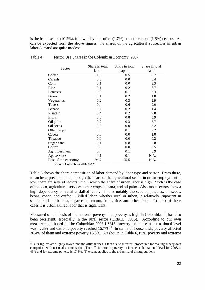
22

is the fruits sector (10.2%), followed by the coffee (1.7%) and other crops (1.6%) sectors. As can be expected from the above figures, the shares of the agricultural subsectors in urban labor demand are quite modest. Table 4. Factor Use Shares in the Colombian Economy, 2007

Sector Share in total

labor Share in total

capital Share in total

land Coffee 1.3 0.5 8.7 Cereals 0.0 0.0 0.4 Corn 0.1 0.0 3.3 Rice 0.1 0.2 8.7 Potatoes 0.3 0.1 3.3 Beans 0.1 0.2 1.0 Vegetables 0.2 0.3 2.9 Tubers 0.4 0.6 9.0 Banana 0.2 0.2 1.4 Plantain 0.4 0.2 9.8 Fruits 0.6 0.8 5.9 Oil palm 0.2 0.3 3.7 Oil seeds 0.0 0.0 3.2 Other crops 0.8 0.1 2.2 Cocoa 0.0 0.0 1.0 Tobacco 0.0 0.0 0.2 Sugar cane 0.1 0.8 33.8 Cotton 0.0 0.0 0.5 Ag. investment 0.4 0.1 0.9 Ag. services 0.1 0.1 N.A. Rest of the economy 94.7 95.5 N.A.

Source: Colombian 2007 SAM Table 5 shows the share composition of labor demand by labor type and sector. From there, it can be appreciated that although the share of the agricultural sector in urban employment is low, there are several sectors within which the share of urban labor is high. Such is the case of tobacco, agricultural services, other crops, banana, and oil palm. Also most sectors show a high dependency on rural unskilled labor. This is notably the case of potatoes, oil seeds, beans, cocoa, and coffee. Skilled labor, whether rural or urban, is relatively important in sectors such as banana, sugar cane, cotton, fruits, rice, and other crops. In most of these cases it is urban skilled labor that is significant. Measured on the basis of the national poverty line, poverty is high in Colombia. It has also been persistent, especially in the rural sector (CRECE, 2005). According to our own measurement, based on the Colombian 2008 LSMS, poverty incidence at the national level was 42.3% and extreme poverty reached 15.7%.11 In terms of households, poverty affected 36.4% of them and extreme poverty 15.5%. As shown in Table 6, rural poverty and extreme

11 Our figures are slightly lower than the official ones, a fact due to different procedures for making survey data compatible with national accounts data. The official rate of poverty incidence at the national level for 2008 is 46% and for extreme poverty is 17.8%. The same applies to the urban- rural disaggregations.

23

poverty are the highest: measured on the basis of individuals, the first reached almost 59% and the second 27%, while the corresponding figures for the urban sector are 37% and 12%. When measured on the basis of households, rural poverty is more than 20 percentage points higher than the urban and extreme poverty is almost 13 percentage points higher. Table 5. Share Composition of Labor Demand by Sector in the Colombian Economy,

2007

Sector Rural labor Urban labor

Unskilled Skilled Unskilled Skilled Coffee 92.1 1.2 6.2 0.4 Cereals 84.4 15.6 Corn 84.9 14.7 0.4 Rice 67.6 14.8 17.6 Potatoes 100.0 Beans 95.2 4.8 Vegetables 82.4 3.2 14.4 Tubers 73.3 26.7 Banana 31.2 33.5 35.2 Plantain 77.2 9.3 13.5 Fruits 69.1 16.7 13.3 0.9 Oil palm 45.8 6.2 33.4 14.6 Oil seeds 100.0 Other crops 30.7 1.9 52.1 15.3 Cocoa 93.3 6.7 Tobacco 21.0 79.0 Sugar cane 54.7 0.8 22.3 22.2 Cotton 62.7 22.9 14.4 Ag. investment 70.8 3.0 19.7 6.6 Ag. services 37.3 62.7 Rest of the economy 4.1 0.8 45.3 49.8

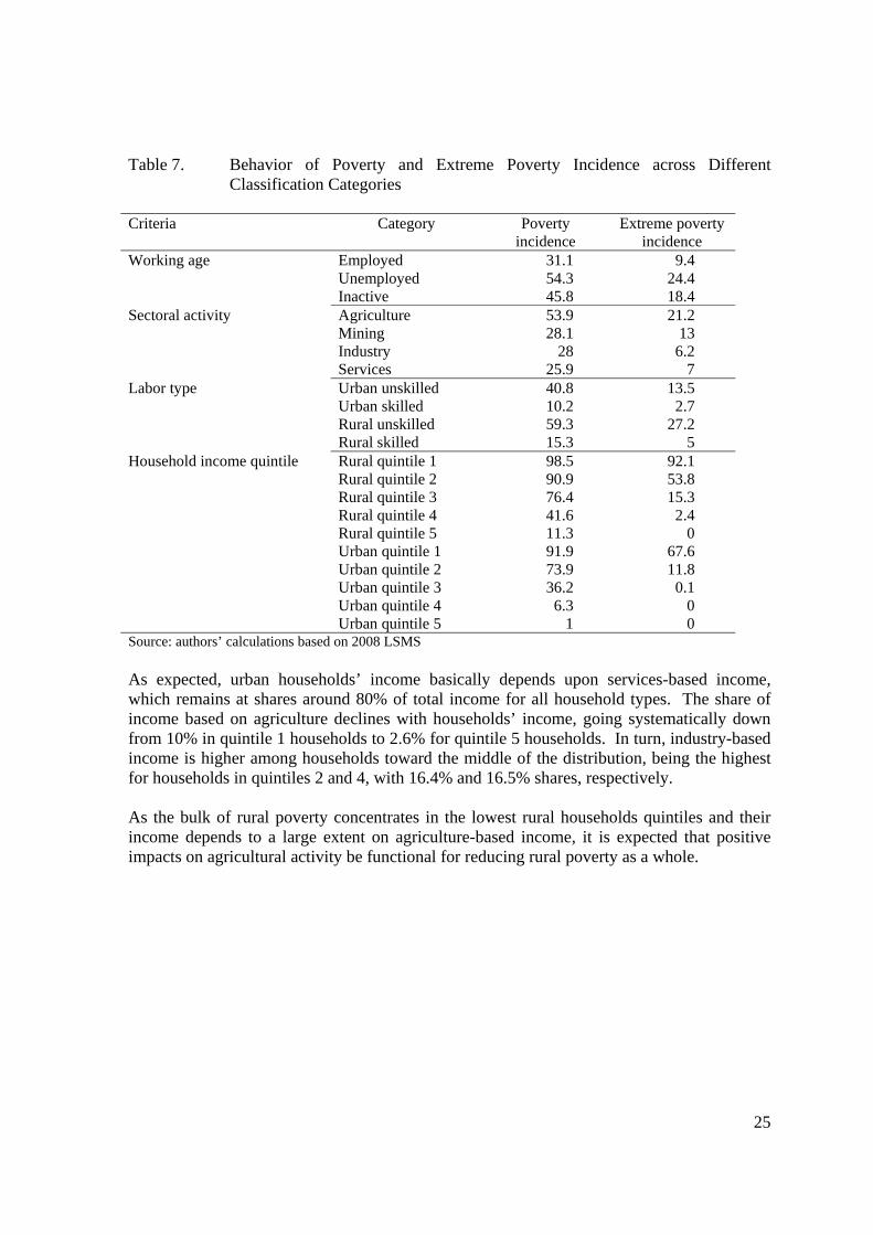
Source: Colombian 2007 SAM The poverty gap (row FGT1 in Table 6) is also highest in the rural sector, both when measured on the basis of individuals and households, meaning that the poor in the rural sector are further below the poverty line and therefore are in need of a larger effort to bring them out of poverty. Lastly, the severity of poverty index (row FGT2) is also highest in the rural sector. It is useful to have a glimpse at the structure of poverty as it helps in understanding the way the policy simulated works its way to have an impact (or lack of) on rural poverty. Table 7 shows the relevant information. Several figures are presented there on the incidence of poverty and of extreme poverty for different categories of individuals. As can be seen, among the population in working age, individuals that are employed show an incidence of poverty of a bit more than 31% and an incidence of extreme poverty of 9.4%. As could be expected, poverty and extreme poverty is higher among unemployed and inactive individuals, being particularly high among unemployed (54.3% poverty and 24.4% extreme poverty). If employed individuals are classified according to the economic sector to which

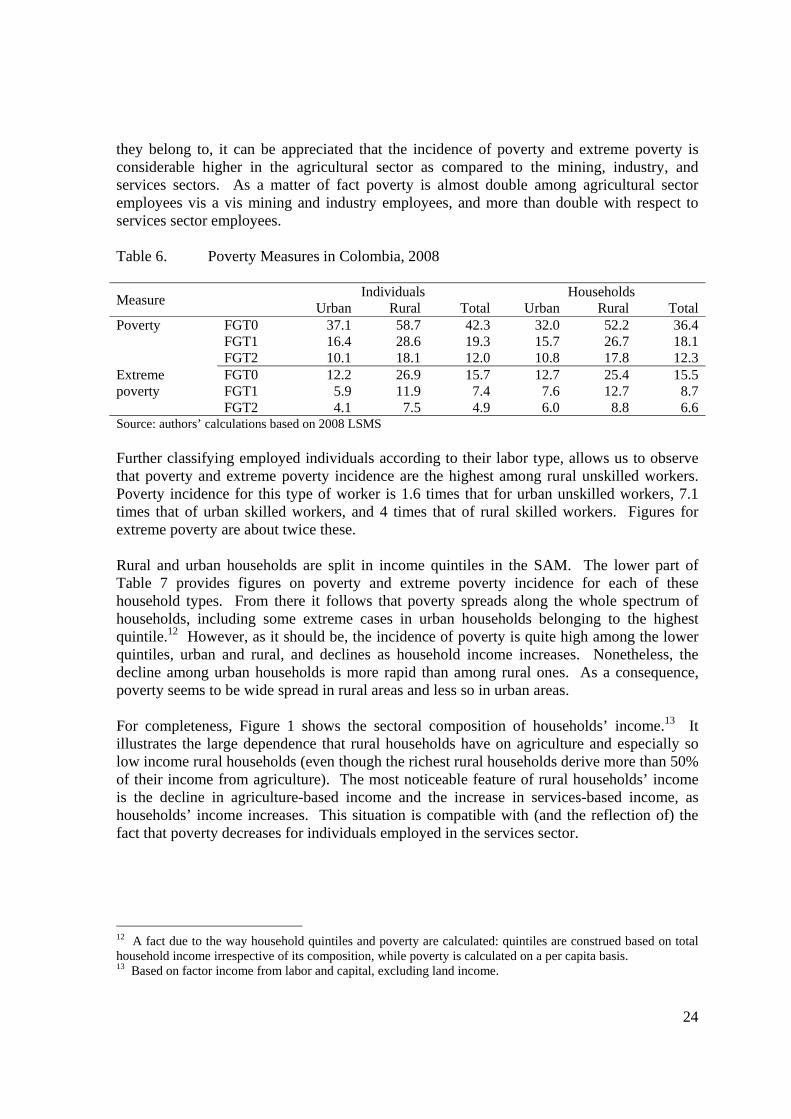
24

they belong to, it can be appreciated that the incidence of poverty and extreme poverty is considerable higher in the agricultural sector as compared to the mining, industry, and services sectors. As a matter of fact poverty is almost double among agricultural sector employees vis a vis mining and industry employees, and more than double with respect to services sector employees. Table 6. Poverty Measures in Colombia, 2008

Measure Individuals Households

Urban Rural Total Urban Rural TotalPoverty FGT0 37.1 58.7 42.3 32.0 52.2 36.4

FGT1 16.4 28.6 19.3 15.7 26.7 18.1FGT2 10.1 18.1 12.0 10.8 17.8 12.3

Extreme poverty

FGT0 12.2 26.9 15.7 12.7 25.4 15.5FGT1 5.9 11.9 7.4 7.6 12.7 8.7FGT2 4.1 7.5 4.9 6.0 8.8 6.6

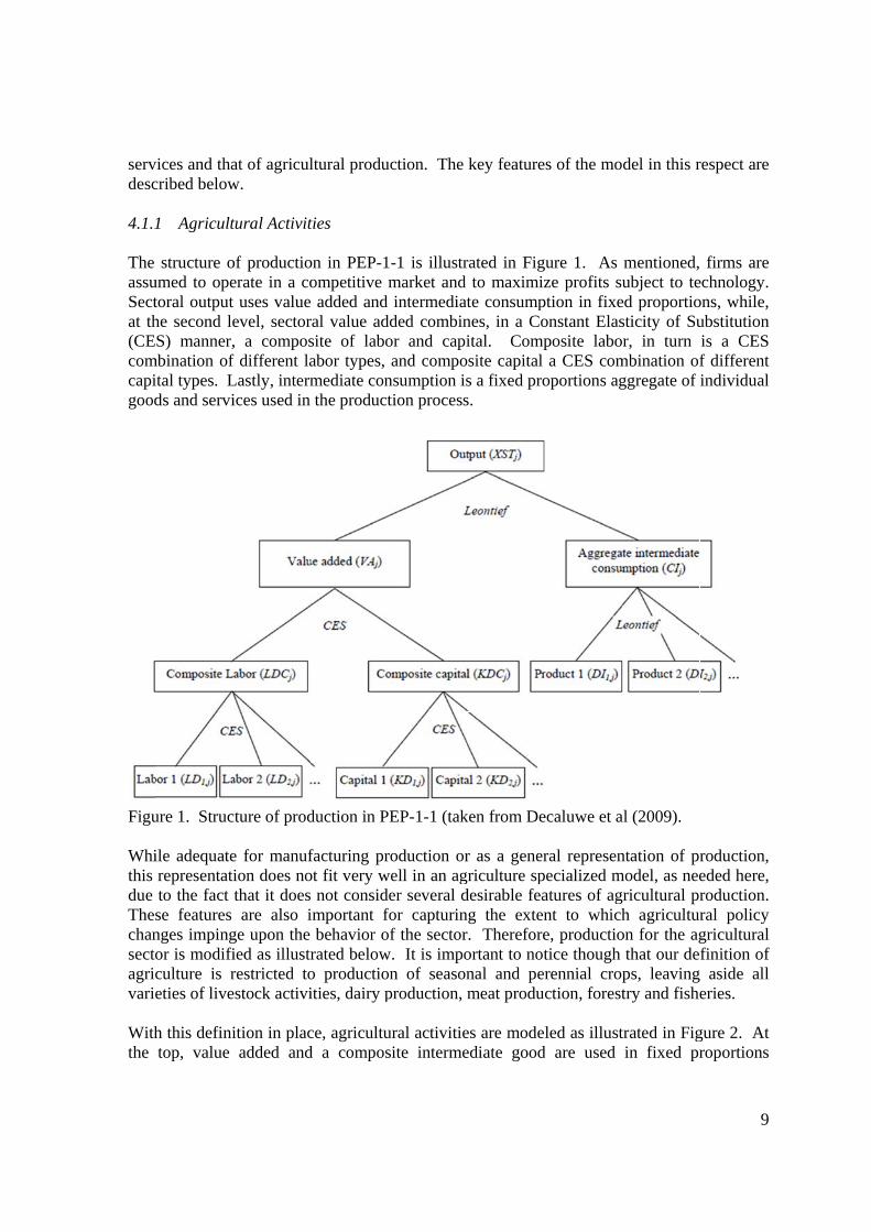
Source: authors’ calculations based on 2008 LSMS Further classifying employed individuals according to their labor type, allows us to observe that poverty and extreme poverty incidence are the highest among rural unskilled workers. Poverty incidence for this type of worker is 1.6 times that for urban unskilled workers, 7.1 times that of urban skilled workers, and 4 times that of rural skilled workers. Figures for extreme poverty are about twice these. Rural and urban households are split in income quintiles in the SAM. The lower part of Table 7 provides figures on poverty and extreme poverty incidence for each of these household types. From there it follows that poverty spreads along the whole spectrum of households, including some extreme cases in urban households belonging to the highest quintile.12 However, as it should be, the incidence of poverty is quite high among the lower quintiles, urban and rural, and declines as household income increases. Nonetheless, the decline among urban households is more rapid than among rural ones. As a consequence, poverty seems to be wide spread in rural areas and less so in urban areas. For completeness, Figure 1 shows the sectoral composition of households’ income.13 It illustrates the large dependence that rural households have on agriculture and especially so low income rural households (even though the richest rural households derive more than 50% of their income from agriculture). The most noticeable feature of rural households’ income is the decline in agriculture-based income and the increase in services-based income, as households’ income increases. This situation is compatible with (and the reflection of) the fact that poverty decreases for individuals employed in the services sector. 12 A fact due to the way household quintiles and poverty are calculated: quintiles are construed based on total household income irrespective of its composition, while poverty is calculated on a per capita basis. 13 Based on factor income from labor and capital, excluding land income.

25

Table 7. Behavior of Poverty and Extreme Poverty Incidence across Different Classification Categories

Criteria Category Poverty

incidence Extreme poverty

incidence Working age Employed 31.1 9.4

Unemployed 54.3 24.4 Inactive 45.8 18.4

Sectoral activity Agriculture 53.9 21.2 Mining 28.1 13 Industry 28 6.2 Services 25.9 7

Labor type Urban unskilled 40.8 13.5 Urban skilled 10.2 2.7 Rural unskilled 59.3 27.2 Rural skilled 15.3 5

Household income quintile Rural quintile 1 98.5 92.1 Rural quintile 2 90.9 53.8 Rural quintile 3 76.4 15.3 Rural quintile 4 41.6 2.4 Rural quintile 5 11.3 0 Urban quintile 1 91.9 67.6 Urban quintile 2 73.9 11.8 Urban quintile 3 36.2 0.1 Urban quintile 4 6.3 0 Urban quintile 5 1 0

Source: authors’ calculations based on 2008 LSMS As expected, urban households’ income basically depends upon services-based income, which remains at shares around 80% of total income for all household types. The share of income based on agriculture declines with households’ income, going systematically down from 10% in quintile 1 households to 2.6% for quintile 5 households. In turn, industry-based income is higher among households toward the middle of the distribution, being the highest for households in quintiles 2 and 4, with 16.4% and 16.5% shares, respectively. As the bulk of rural poverty concentrates in the lowest rural households quintiles and their income depends to a large extent on agriculture-based income, it is expected that positive impacts on agricultural activity be functional for reducing rural poverty as a whole.

26

Source: authors’ calculations based on 2008 LSMS

Figure 1. Sectoral Composition of Households’ Income by Household Type 6. Results For easiness of exposition results from the two models are presented independently. We first look at the results from the CGE model, and then to the ones from the micro model. 6.1 CGE Results As mentioned before, only one scenario is run with the CGE model, that of implementation of the AIS program as (approximately) done during 2008. For this, total amounts directly or indirectly spent by the government for granting the different subsidy types, independently as to whether they were granted to small, medium or large farmers, are split by crop (following the sectoral composition of the SAM) according to their participation within the SCL component devoted for planting new hectares. In other words, we start from total expending figures for granting subsidies under the four modalities (numerals a. to d.) described in sub-section 4.1.7 above. Since we do not have the split of these figures per crop type, we retort to each crop’s share in credit granted through the SCL for new planting, and use it across the remaining three subsidy types. Clearly, the procedure does not give any assurance that we are assigning to each crop the share it really has per subsidy type, so the exercise is meant as the best plausible approximation of the likely effects of the program. As the required information will become available, more precise figures will be used.14 14 The trouble for getting to the right information is that the issue has become highly politically sensible. As of the end of 2009 and beginning of 2010, a noticeable political scandal arose, when it was made public by some media that there was a high concentration of some of the benefits of the program in a small group of rich farmers. This was so not only due to the fact that eligibility criteria was more difficult to meet by small farmers, but also because some large farmers illegally divided their projects into seemingly independent and

 ‐

 10.00

 20.00

 30.00

 40.00

 50.00

 60.00

 70.00

 80.00

 90.00

RuralQ1

RuralQ2

RuralQ3

RuralQ4

RuralQ5

UrbanQ1

UrbanQ2

UrbanQ3

UrbanQ4

UrbanQ5

Agriculture Mining Industry Services

27

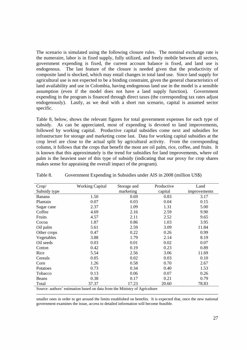
The scenario is simulated using the following closure rules. The nominal exchange rate is the numeraire, labor is in fixed supply, fully utilized, and freely mobile between all sectors, government expending is fixed, the current account balance is fixed, and land use is endogenous. The last feature of the closure is needed given that the productivity of composite land is shocked, which may entail changes in total land use. Since land supply for agricultural use is not expected to be a binding constraint, given the general characteristics of land availability and use in Colombia, having endogenous land use in the model is a sensible assumption (even if the model does not have a land supply function). Government expending in the program is financed through direct taxes (the corresponding tax rates adjust endogenously). Lastly, as we deal with a short run scenario, capital is assumed sector specific. Table 8, below, shows the relevant figures for total government expenses for each type of subsidy. As can be appreciated, most of expending is devoted to land improvements, followed by working capital. Productive capital subsidies come next and subsidies for infrastructure for storage and marketing come last. Data for working capital subsidies at the crop level are close to the actual split by agricultural activity. From the corresponding column, it follows that the crops that benefit the most are oil palm, rice, coffee, and fruits. It is known that this approximately is the trend for subsidies for land improvements, where oil palm is the heaviest user of this type of subsidy (indicating that our proxy for crop shares makes sense for appraising the overall impact of the program). Table 8. Government Expending in Subsidies under AIS in 2008 (million US$) Crop/ Subsidy type

Working Capital Storage and marketing

Productive capital

Land improvements

Banana 1.50 0.69 0.83 3.17 Plantain 0.07 0.03 0.04 0.15 Sugar cane 2.37 1.09 1.31 5.00 Coffee 4.69 2.16 2.59 9.90 Fruits 4.57 2.11 2.52 9.65 Cocoa 1.87 0.86 1.03 3.95 Oil palm 5.61 2.59 3.09 11.84 Other crops 0.47 0.22 0.26 0.99 Vegetables 3.88 1.79 2.14 8.19 Oil seeds 0.03 0.01 0.02 0.07 Cotton 0.42 0.19 0.23 0.89 Rice 5.54 2.56 3.06 11.69 Cereals 0.05 0.02 0.03 0.10 Corn 1.26 0.58 0.70 2.67 Potatoes 0.73 0.34 0.40 1.53 Tobacco 0.13 0.06 0.07 0.26 Beans 0.38 0.17 0.21 0.79 Total 37.37 17.23 20.60 78.83 Source: authors’ estimation based on data from the Ministry of Agriculture smaller ones in order to get around the limits established on benefits. It is expected that, once the new national government examines the issue, access to detailed information will become feasible.

28

Government expenses are used to endogenously calculate rates of subsidization for each agricultural activity and these rates affect activities in the way previously described (sub-section 4.17). The calculated rates of subsidization, with respect to the whole of each agricultural activity are presented in Table 9. As shown, most subsidization rates on working capital and storage and marketing, are small and only in the case of the subsidy on working capital for the cocoa sector is higher than one percent. Although in the case of subsidies on productive capital rates tend also to be low, there are a few cases in which they are relatively sizeable: corn and cocoa. In the case of land improvements we have to sources of shocks. One refers to the implicit subsidy on land rents, accruing from the irrigation subsidy program and the other refers to the increase in land productivity due to irrigation. The first entails percentage subsidy rates in general higher than in the other schemes, with an average rate of almost 5.5%. However, as follows from the figures, there is considerable heterogeneity across sectors, with cocoa, oil palm, and vegetables showing high subsidy rates and plantain, oil seeds, sugar cane, and cereals showing quite low rates. As there is a correlation between this subsidy and expected productivity improvements, the activities that get the highest land rent subsidies show the highest productivity gains. As an average, productivity gains are around 9% in yields, while the highest are in the order of 22% and the lowest in the order of 0.4%. Table 9. Percentage Rates of Subsidization per Subsidy Type and Agricultural Activity

(calculated on the whole activity)

Crop/Subsidy Rate

On Working Capital

On Storage and Marketing: On Productive

Capital

On Land Improvements: Importable-Domestic

Exportable Land Rent

Productivity

Coffee 0.24 0.11 0.00 0.40 4.49 7.13 Cereals 0.12 0.00 0.00 0.16 0.96 1.53 Corn 0.49 0.06 0.06 6.94 3.13 4.97 Rice 0.69 0.31 0.39 1.34 5.43 8.63 Potatoes 0.09 0.04 0.04 0.23 1.80 2.86 Beans 0.13 0.05 0.05 0.10 3.26 5.18 Vegetables 0.55 0.24 0.24 0.49 12.46 19.80 Banana 0.25 0.11 0.11 0.39 9.05 14.38 Plantain 0.01 0.00 0.00 0.01 0.06 0.09 Fruits 0.26 0.11 0.11 0.24 6.52 10.37 Oil palm 1.42 0.00 0.00 0.92 13.18 20.94 Oil seeds 0.02 0.01 0.00 0.04 0.08 0.13 Other crops 0.04 0.02 0.02 0.23 1.73 2.74 Cocoa 2.28 0.74 0.65 5.34 16.76 26.64 Tobacco 0.32 0.11 0.11 0.41 6.82 10.84 Sugar cane 0.21 0.00 0.00 0.13 0.57 0.90 Cotton 0.60 0.13 0.13 1.85 6.94 11.03 Source: authors’ estimation based on data from the Ministry of Agriculture As can be inferred, the above rates are low as they are calculated with respect to the whole of each sector but may be quite sizeable considered at the individual level. This is especially true of expending on land improvements as follows from the magnitude of the average

29

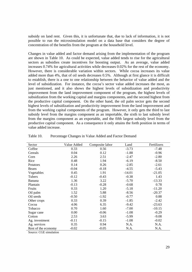
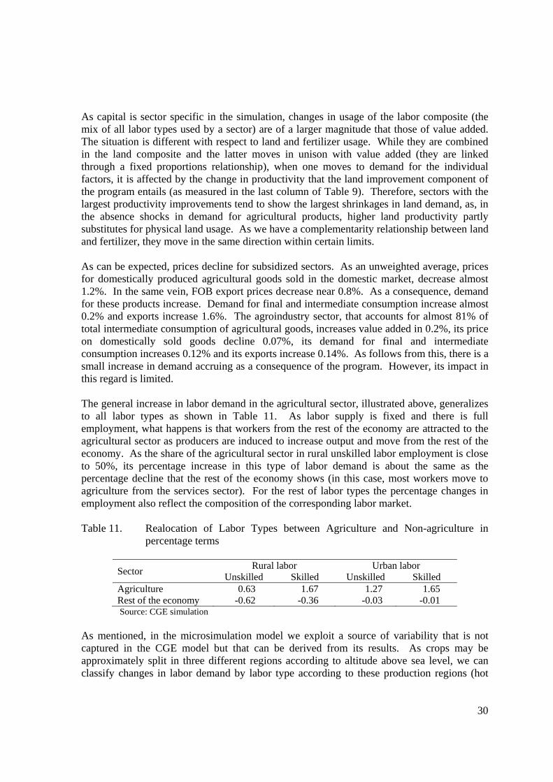
subsidy on land rent. Given this, it is unfortunate that, due to lack of information, it is not possible to run the microsimulation model on a data base that considers the degree of concentration of the benefits from the program at the household level. Changes in value added and factor demand arising from the implementation of the program are shown in Table 10. As could be expected, value added tends to rise for the agricultural sectors as subsidies create incentives for boosting output. As an average, value added increases 0.74% for agricultural activities while decreases 0.02% for the rest of the economy. However, there is considerable variation within sectors. While cocoa increases its value added more than 4%, that of oil seeds decreases 0.5%. Although at first glance it is difficult to establish, there is a one to one relationship between the behavior of value added and the level of subsidization. For instance, the cocoa’s sector value added increases the most, as just mentioned, and it also shows the highest levels of subsidization and productivity improvement from the land improvement component of the program, the highest levels of subsidization from the working capital and margins components, and the second highest from the productive capital component. On the other hand, the oil palm sector gets the second highest levels of subsidization and productivity improvement from the land improvement and from the working capital components of the program. However, it only gets the third to last subsidy level from the margins component as an importable, the sixth to last subsidy level from the margins component as an exportable, and the fifth largest subsidy level from the productive capital component. As a consequence it only attains the forth position in terms of value added increase. Table 10. Percentage Changes in Value Added and Factor Demand Sector Value Added Composite labor Land Fertilizers Coffee 0.33 0.56 -3.73 -7.48 Cereals 0.04 0.12 -1.88 -0.96 Corn 2.26 2.51 -2.47 -2.80 Rice 0.48 1.94 -6.19 -8.50 Potatoes 0.14 0.26 -2.85 -2.61 Beans -0.04 -0.18 -4.55 -5.43 Vegetables 0.45 1.91 -14.01 -21.05 Tubers -0.12 -0.43 -0.38 1.43 Banana 1.36 3.22 -5.70 -13.33 Plantain -0.13 -0.28 -0.68 0.78 Fruits 0.33 1.20 -5.18 -11.20 Oil palm 1.52 5.88 -8.56 -20.37 Oil seeds -0.50 -1.92 -0.77 0.88 Other crops 0.33 0.39 -1.85 -2.42 Cocoa 4.06 6.35 -9.42 -23.63 Tobacco 0.70 1.60 -7.00 -10.15 Sugar cane 0.00 -0.06 -1.08 -0.29 Cotton 2.53 3.63 -5.99 -9.08 Ag. investment -0.11 -0.15 -1.08 -0.02 Ag. services 0.35 0.94 N.A. N.A.Rest of the economy -0.02 -0.05 N.A. N.A.Source: CGE simulation

30

As capital is sector specific in the simulation, changes in usage of the labor composite (the mix of all labor types used by a sector) are of a larger magnitude that those of value added. The situation is different with respect to land and fertilizer usage. While they are combined in the land composite and the latter moves in unison with value added (they are linked through a fixed proportions relationship), when one moves to demand for the individual factors, it is affected by the change in productivity that the land improvement component of the program entails (as measured in the last column of Table 9). Therefore, sectors with the largest productivity improvements tend to show the largest shrinkages in land demand, as, in the absence shocks in demand for agricultural products, higher land productivity partly substitutes for physical land usage. As we have a complementarity relationship between land and fertilizer, they move in the same direction within certain limits. As can be expected, prices decline for subsidized sectors. As an unweighted average, prices for domestically produced agricultural goods sold in the domestic market, decrease almost 1.2%. In the same vein, FOB export prices decrease near 0.8%. As a consequence, demand for these products increase. Demand for final and intermediate consumption increase almost 0.2% and exports increase 1.6%. The agroindustry sector, that accounts for almost 81% of total intermediate consumption of agricultural goods, increases value added in 0.2%, its price on domestically sold goods decline 0.07%, its demand for final and intermediate consumption increases 0.12% and its exports increase 0.14%. As follows from this, there is a small increase in demand accruing as a consequence of the program. However, its impact in this regard is limited. The general increase in labor demand in the agricultural sector, illustrated above, generalizes to all labor types as shown in Table 11. As labor supply is fixed and there is full employment, what happens is that workers from the rest of the economy are attracted to the agricultural sector as producers are induced to increase output and move from the rest of the economy. As the share of the agricultural sector in rural unskilled labor employment is close to 50%, its percentage increase in this type of labor demand is about the same as the percentage decline that the rest of the economy shows (in this case, most workers move to agriculture from the services sector). For the rest of labor types the percentage changes in employment also reflect the composition of the corresponding labor market. Table 11. Realocation of Labor Types between Agriculture and Non-agriculture in

percentage terms

Sector Rural labor Urban labor

Unskilled Skilled Unskilled Skilled Agriculture 0.63 1.67 1.27 1.65 Rest of the economy -0.62 -0.36 -0.03 -0.01 Source: CGE simulation

As mentioned, in the microsimulation model we exploit a source of variability that is not captured in the CGE model but that can be derived from its results. As crops may be approximately split in three different regions according to altitude above sea level, we can classify changes in labor demand by labor type according to these production regions (hot

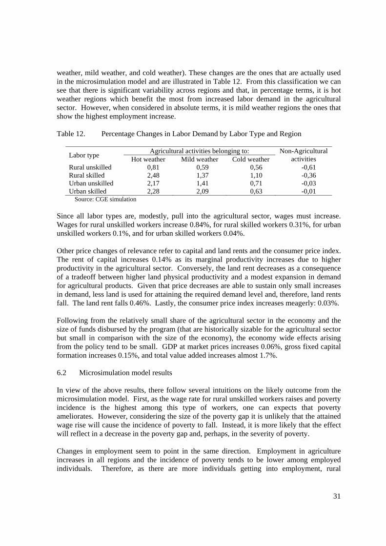
31

weather, mild weather, and cold weather). These changes are the ones that are actually used in the microsimulation model and are illustrated in Table 12. From this classification we can see that there is significant variability across regions and that, in percentage terms, it is hot weather regions which benefit the most from increased labor demand in the agricultural sector. However, when considered in absolute terms, it is mild weather regions the ones that show the highest employment increase. Table 12. Percentage Changes in Labor Demand by Labor Type and Region

Labor type Agricultural activities belonging to: Non-Agricultural

activities Hot weather Mild weather Cold weather Rural unskilled 0,81 0,59 0,56 -0,61 Rural skilled 2,48 1,37 1,10 -0,36 Urban unskilled 2,17 1,41 0,71 -0,03 Urban skilled 2,28 2,09 0,63 -0,01

Source: CGE simulation Since all labor types are, modestly, pull into the agricultural sector, wages must increase. Wages for rural unskilled workers increase 0.84%, for rural skilled workers 0.31%, for urban unskilled workers 0.1%, and for urban skilled workers 0.04%. Other price changes of relevance refer to capital and land rents and the consumer price index. The rent of capital increases 0.14% as its marginal productivity increases due to higher productivity in the agricultural sector. Conversely, the land rent decreases as a consequence of a tradeoff between higher land physical productivity and a modest expansion in demand for agricultural products. Given that price decreases are able to sustain only small increases in demand, less land is used for attaining the required demand level and, therefore, land rents fall. The land rent falls 0.46%. Lastly, the consumer price index increases meagerly: 0.03%. Following from the relatively small share of the agricultural sector in the economy and the size of funds disbursed by the program (that are historically sizable for the agricultural sector but small in comparison with the size of the economy), the economy wide effects arising from the policy tend to be small. GDP at market prices increases 0.06%, gross fixed capital formation increases 0.15%, and total value added increases almost 1.7%. 6.2 Microsimulation model results In view of the above results, there follow several intuitions on the likely outcome from the microsimulation model. First, as the wage rate for rural unskilled workers raises and poverty incidence is the highest among this type of workers, one can expects that poverty ameliorates. However, considering the size of the poverty gap it is unlikely that the attained wage rise will cause the incidence of poverty to fall. Instead, it is more likely that the effect will reflect in a decrease in the poverty gap and, perhaps, in the severity of poverty. Changes in employment seem to point in the same direction. Employment in agriculture increases in all regions and the incidence of poverty tends to be lower among employed individuals. Therefore, as there are more individuals getting into employment, rural

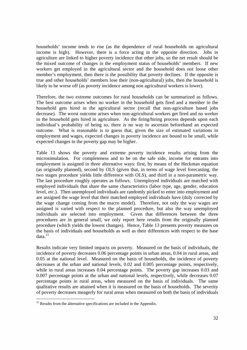
32

households’ income tends to rise (as the dependence of rural households on agricultural income is high). However, there is a force acting in the opposite direction. Jobs in agriculture are linked to higher poverty incidence that other jobs, so the net result should be the mixed outcome of changes in the employment status of households’ members. If new workers get employed in the agricultural sector and the household does not loose other member’s employment, then there is the possibility that poverty declines. If the opposite is true and other households’ members lose their (non-agricultural) jobs, then the household is likely to be worse off (as poverty incidence among non agricultural workers is lower). Therefore, the two extreme outcomes for rural households can be summarized as follows. The best outcome arises when no worker in the household gets fired and a member in the household gets hired in the agricultural sector (recall that non-agriculture based jobs decrease). The worst outcome arises when non-agricultural workers get fired and no worker in the household gets hired in agriculture. As the firing/hiring process depends upon each individual’s probability of being so, there is no way to ascertain beforehand an expected outcome. What is reasonable is to guess that, given the size of estimated variations in employment and wages, expected changes in poverty incidence are bound to be small, while expected changes in the poverty gap may be higher. Table 13 shows the poverty and extreme poverty incidence results arising from the microsimulation. For completeness and to be on the safe side, income for entrants into employment is assigned in three alternative ways: first, by means of the Heckman equation (as originally planned), second by OLS (given that, in terms of wage level forecasting, the two stages procedure yields little difference with OLS), and third in a non-parametric way. The last procedure roughly operates as follows. Unemployed individuals are matched with employed individuals that share the same characteristics (labor type, age, gender, education level, etc.). Then unemployed individuals are randomly picked to enter into employment and are assigned the wage level that their matched employed individuals have (duly corrected by the wage change coming from the macro model). Therefore, not only the way wages are assigned is varied with respect to the planned procedure, but also the way unemployed individuals are selected into employment. Given that differences between the three procedures are in general small, we only report here results from the originally planned procedure (which yields the lowest changes). Hence, Table 13 presents poverty measures on the basis of individuals and households as well as their differences with respect to the base data.15 Results indicate very limited impacts on poverty. Measured on the basis of individuals, the incidence of poverty decreases 0.06 percentage points in urban areas, 0.04 in rural areas, and 0.05 at the national level. Measured on the basis of households, the incidence of poverty decreases at the urban and national levels, 0.02 and 0.005 percentage points, respectively, while in rural areas increases 0.04 percentage points. The poverty gap increases 0.03 and 0.007 percentage points at the urban and national levels, respectively, while decreases 0.07 percentage points in rural areas, when measured on the basis of individuals. The same qualitative results are attained when it is measured on the basis of households. The severity of poverty decreases meagerly for rural areas when measured on both the basis of individuals 15 Results from the alternative specifications are included in the Appendix.

33

and households and increases for urban areas and at the national level. Extreme poverty decreases in all counts (incidence, poverty gap, and severity) when measured on the basis of individuals, while only in terms of the poverty gap and the severity of poverty when measured on the basis of households. Table 13. Poverty and Extreme Poverty Results from the Microsimulation

Measure Individuals Households

Urban Rural Total Urban Rural TotalPoverty FGT0 37.06 58.66 42.21 31.95 52.26 36.36

Difference -0.057 -0.037 -0.053 -0.019 0.042 -0.005FGT1 16.40 28.53 19.29 15.71 26.65 18.09Difference 0.029 -0.065 0.007 0.013 -0.017 0.008FGT2 10.13 18.07 12.03 10.83 17.83 12.35Difference 0.038 -0.050 0.017 0.024 -0.017 0.015

Extreme poverty

FGT0 12.24 26.89 15.73 12.70 25.46 15.47Difference 0.049 -0.028 0.031 0.005 0.078 0.021FGT1 5.99 11.86 7.39 7.67 12.70 8.77Difference 0.047 -0.039 0.027 0.037 -0.019 0.025FGT2 4.14 7.52 4.95 6.05 8.83 6.65Difference 0.042 -0.014 0.029 0.040 -0.017 0.028

Source: microsimulation model These results deserve some comments. That rural poverty incidence decreases when measured at the individuals level and do not do so when measured at the household level is a feature associated with the composition of households. While wages for all labor types increase, wages for the rural categories of work increase the most. However, households’ income, including that of those in the rural sector, is dependent upon income originated in agricultural and non-agricultural activities. While the employment in the former increases, it decreases in the rest of the economy, so as rural households may have members whose income comes from non-agricultural activities, they face the possibility of losing their jobs. To see this, let remember that low income rural households derive most of their income from agricultural activities (recall Figure 1) –either in the form of wages, or other factors’ income. Given this, with the general increase in agricultural activity we can expect these households’ income to rise. However, this is not necessarily the case as figures shown in Table 14 indicate. There, households have been ordered from highest to lowest poverty incidence in the base data. As can be appreciated poverty incidence either does not vary or slightly increases among the poorest households. It is only in the case of households toward the middle of the distribution that poverty actually decreases, in particular from rural quintile 3 to rural quintile 4. As wages have small variations, their ability to move households out of poverty is limited and it is entry and exit from employment what may help make a difference. It turns out that members of households with the lowest income levels have also the lowest probabilities of being hired and the highest probabilities of being fired; therefore, they cannot take advantage of the changes arising from the shock. As sown in the table, poverty incidence only

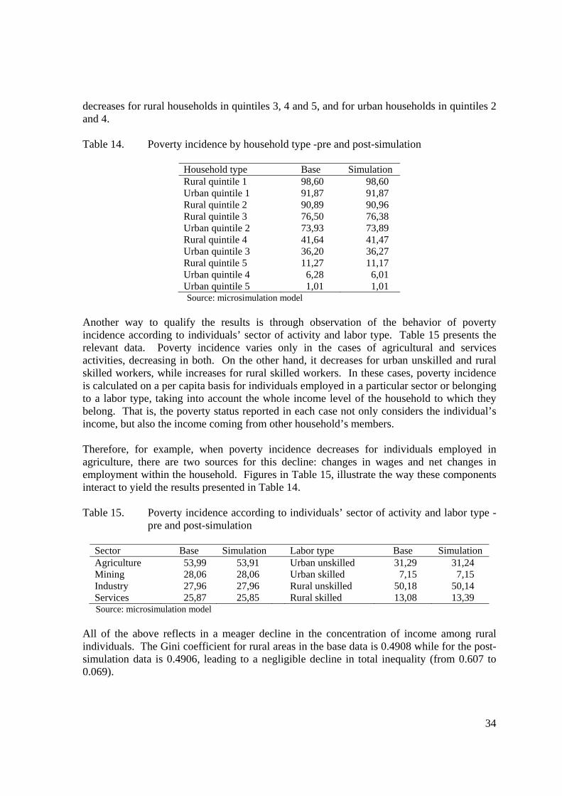
34

decreases for rural households in quintiles 3, 4 and 5, and for urban households in quintiles 2 and 4. Table 14. Poverty incidence by household type -pre and post-simulation

Household type Base Simulation Rural quintile 1 98,60 98,60 Urban quintile 1 91,87 91,87 Rural quintile 2 90,89 90,96 Rural quintile 3 76,50 76,38 Urban quintile 2 73,93 73,89 Rural quintile 4 41,64 41,47 Urban quintile 3 36,20 36,27 Rural quintile 5 11,27 11,17 Urban quintile 4 6,28 6,01 Urban quintile 5 1,01 1,01 Source: microsimulation model

Another way to qualify the results is through observation of the behavior of poverty incidence according to individuals’ sector of activity and labor type. Table 15 presents the relevant data. Poverty incidence varies only in the cases of agricultural and services activities, decreasing in both. On the other hand, it decreases for urban unskilled and rural skilled workers, while increases for rural skilled workers. In these cases, poverty incidence is calculated on a per capita basis for individuals employed in a particular sector or belonging to a labor type, taking into account the whole income level of the household to which they belong. That is, the poverty status reported in each case not only considers the individual’s income, but also the income coming from other household’s members. Therefore, for example, when poverty incidence decreases for individuals employed in agriculture, there are two sources for this decline: changes in wages and net changes in employment within the household. Figures in Table 15, illustrate the way these components interact to yield the results presented in Table 14. Table 15. Poverty incidence according to individuals’ sector of activity and labor type -

pre and post-simulation

Sector Base Simulation Labor type Base Simulation Agriculture 53,99 53,91 Urban unskilled 31,29 31,24 Mining 28,06 28,06 Urban skilled 7,15 7,15 Industry 27,96 27,96 Rural unskilled 50,18 50,14 Services 25,87 25,85 Rural skilled 13,08 13,39 Source: microsimulation model

All of the above reflects in a meager decline in the concentration of income among rural individuals. The Gini coefficient for rural areas in the base data is 0.4908 while for the post-simulation data is 0.4906, leading to a negligible decline in total inequality (from 0.607 to 0.069).

35

In the simulation, as mentioned, it was assumed that the yield gap between irrigated and non-irrigated land was the same across agricultural activities and equivalent to a 20% wedge. It also was calculated, based on actual data from the AIS program, that the average rate of subsidy for irrigation projects is 0.755. While we currently do not have data to make the yield gap specific to each agricultural activity, it seems convenient to test how results change if both the yield gap and the subsidy rate change. Results from several variations of these parameters for both the macro and micro models are presented in the Appendix. From there (Tables A.2 and A.3) it can be appreciated that there are not wide variations in results, both from the macro and micro models. The best possible decrease in rural poverty yields a decrease of 0.19 percentage points when measured on the basis of individuals and 0.08 when measured on the basis of households, while the worst outcome yields practically no change in rural poverty when measured at the individuals level and a slight increase, 0.07 percentage points, when measured at the household level. 7. Conclusions

We attempt to provide an estimate of the sectoral and rural poverty impacts of the newly implemented reforms to Colombian agricultural policy (the Agriculture, Secured Income, AIS Program). For this we use a computable general equilibrium model specialized in the agricultural sector, sequentially with a microsimulation model. Results indicate that although sizable for Colombian standards, especially in terms of public sector budget allocation, the program is relatively weak when confronted with the size of the agricultural sector. This reflects in relatively low subsidy rates at the sectoral level and in negligible impacts from the program at the aggregated economy level. These facts call attention to potentially important distributive issues. While the size of the program is in general small for having significant agriculture-wide impacts, it is sizable enough to make up for significant subsidization at the individual farmer level. Therefore, access to the program is key in determining its distributive implications. It is known that resources allocated to medium size and large farmers are exhausted at a rapid pace, once funds are allocated to the program by the government, while demand for funds by small farmers is sluggish. It is also known that disbursements for projects submitted by medium size and large farmers make up for the largest share of funds. In view of these, it is likely that the program may be enhancing the degree of concentration of agricultural activity. While data availability precludes us from appraising this issue, there is no doubt that this is an important research area for Colombia. At the sectoral level we find relatively small impacts on value added, although with high variability among sectors. As expected, value added changes depend upon the level of subsidization that a sector attains; however, the largest impact comes from subsidies devoted to irrigation as they affect not only the cost of using land but also its productivity. As there is nothing in the policy that affects the demand side, higher productivity reflects partly in increased value added and in lower demand for land, since price declines induced by higher

36

productivity do not enhance demand enough. As a consequence, land rents may decline negatively affecting income of households owning land plots. In the macro model there are two constraints impinging upon labor mobility. Capital is sector specific and land mobility is sluggish across crops. These features have an impact on agricultural response and also help in attaining limited reallocation of workers within agriculture and from the rest of the economy. We deem these features as realistically representing characteristics of Colombian agriculture and therefore do not expect that the program will have significant impacts on labor reallocation. Consistently, results show that wage changes induced by increased demand in the agricultural sector are bound to be small. With small wage and capital rent increases, small reductions in land rents, and limited labor reallocation, poverty impacts are small. Rural poverty incidence decrease less than 1 per cent and the same happens with the poverty gap. Additionally, poverty reduction concentrates in households located toward the middle of the income distribution, in particular in rural households belonging to income quintiles 2, 3, and 4 (and in urban households in quintile 2). The above relates to the ability of individuals to get into employment and to their vulnerability to get fired. Seemingly, individuals pertaining to low income households are both, less likely to land employments and more prone to be fired, so they benefit the least from changes induced by the implementation of the program. In sum, as implemented, AIS seems to have a limited capability for reaching the objectives for which it was designed. As an instrument for smoothing the adverse impact of increased foreign competition it appears to fall short as its estimated impacts on production are low. On the other hand, as an instrument to boost agricultural productivity and competitiveness it shows more promise but lacks reach and may induce greater concentration of agricultural activity at the expense of small farmers. Lastly, although it is not one of its stated objectives, its impact on poverty reduction seems to be very limited.

37

References Baltzer, K. and J. Kloverpris (2008) Improving the land use specification in the GTAP model, Institute of Food and Resource Economics Working Paper 02/08, February. Bussolo, M., and J. Lay (2005) Globalization and poverty changes in Colombia. In Globalization and poverty channels and policy responses, ed. M. Bussolo and J. Round, 195–227. London: Routledge Colombian Congress (2007) Law 1133 from April 9, in Official Diary No. 46.595 from April 10, 2007 CRECE (2005) Pobreza Rural: Evaluación y Diagnóstico de las Políticas Nacionales. Informe Final para la Misión para la Erradicación de la Pobreza y la Desigualdad. DANE (2009) Informe de la Misión para el empalme de las series de empleo, pobreza y desigualdad, Resultados Fase I: Empalme de las series de mercado laboral, pobreza y desigualdad, Agosto. Darwin, R, M. Tsigas, J. Lewandrowski, and A. Raneses (1995) World Agriculture and Climate Change. Economic Adaptations, Agricultural Economic Report No. 703, United States Department of Agriculture-ERS, June, Washington. Decaluwe, B., A. Lemelin, H. Maisonnave, and V. Robichaud (2009) The PEP Standard Computable General Equilibrium Model. Single-Country, Static Version. PEP-1-1, Second Revised Edition, Poverty and Economic Policy (PEP) Research Network, October. Espinosa, A. (ed.) (2005) La Agricultura Colombiana Frente al Tratado de Libre Comercio con Estados Unidos, Ministerio de Agricultura – Bolsa Nacional Agropecuaria, Bogotá, D.C. Ferreira-Filho, J. and M. Horridge (2004) Economic Integration, Poverty, and Regional Inequality in Brazil. Paper presented at the 7th Annual Conference on Global Economic Analysis. Guterman, L. (2007) Distortions to Agricultural Incentives in Colombia, Agricultural Distortions Working Paper 14, World Bank Development Research Group’s project on Distortions to Agricultural Incentives, December Hertel, T., H.L. Lee, S. Rose, and B. Sohngen (2008) Modeling Land-use Related Greenhouse Gas Sources and Sinks and their Mitigation Potential, GTAP Working Paper No. 44. Hertel, T., S. Rose, and R. Tol (2007) Land Use in Computable General Equilibrium Models: An Overview, GTAP Working Paper No. 39.

38

Ministry of Agriculture and Rural Development- MADR (2008) Reactivación agropecuaria y mayor bienestar en el campo. Memorias 2007-2008. Andrés F. Arias L. Ministro. Ministry of Trade, Industry, and Tourism. Colombia. Comercio Exterior de Colombia, Oficina de Estudios Económicos, available at http://www.mincomercio.gov.co/eContent/newsdetail.asp?id=761&idcompany=1 Núñez, J. y Espinosa, S. (2005) No siempre pobres, no siempre ricos: vulnerabilidad en Colombia, Documentos CEDE, No. 15, March Savard, L. (2003) “Poverty and Income Distribution in a CGE-Household Micro-Simulation Model: Top-Down/Bottom Up Approach,” mimeo, International Development Research Centre. USTR (2005) Interim Environmental Review. U.S.-Andean Free Trade Agreement. Office of the U.S. Trade Representative, February Van Meijl, H., T. van Rheenen, A. Tabeau, and B. Eickhout (2006) The impact of different policy environments on agricultural land use in Europe, in Agriculture, Ecosystems & Environment, 114, 21-38 World Bank World Development Indicators Database. World Bank (2008) Distortions to Agricultural Incentives in Latin America, Kym Anderson and Alberto Valdés (eds.), Washington WTO (2006) Trade Policy Review. Report by the Secretariat. Colombia, WT/TPR/172, Geneva

39

APPENDIX

A. Implementation of agricultural production The structure used for representing agricultural production is done through the following set of equations: = ∗ = ∗ = ∗ = ∗ where: = = = = = − = ( − ) = ( − ) = ( − ) = ( − − ) = + (1 − )

where: = = = ( − ) = ℎ ( − ) = ( − );−1 < < ∞ =

= (1 − )

where: = . = .

40

= = ( − ); 0 < < 1 = 1 −

= + (1 − )

where: = = = ( − − ) = ℎ ( − − ) = ( − − );−1 < < ∞ = 1 −

= , ,

, = , ,

= , ,

, = , ,

where: , = , = = . = . = . , = = ( − ) = ( − ) , = ℎ ( − ) , = ℎ ( − ) = ( − ); −1 < < ∞

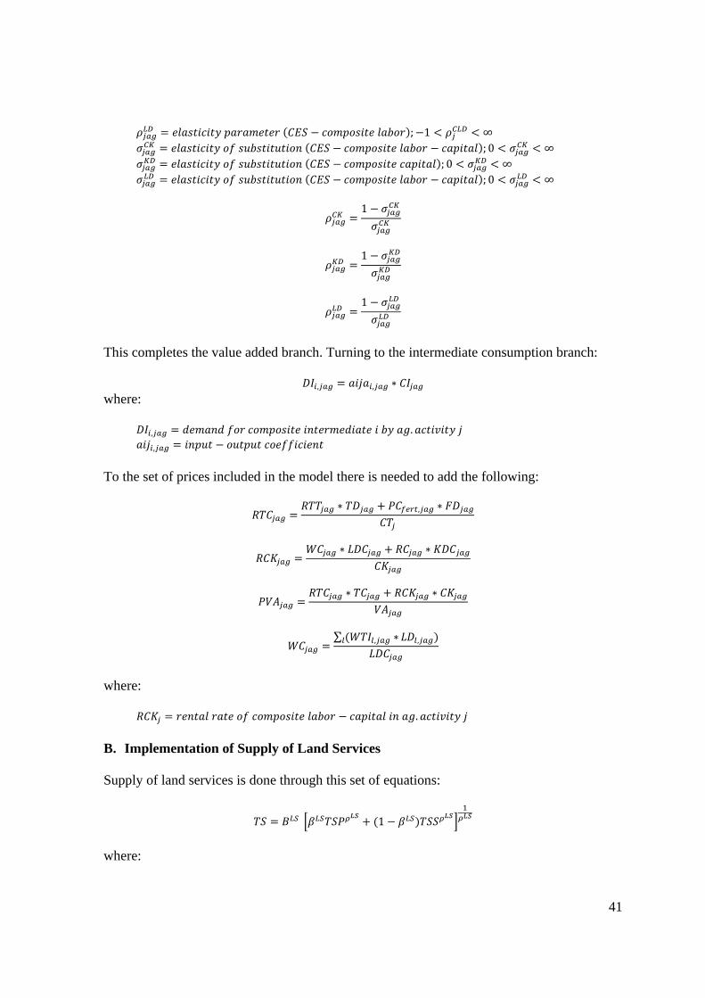
41

= ( − ); −1 < < ∞ = ( − − ); 0 < < ∞ = ( − ); 0 < < ∞ = ( − − ); 0 < < ∞ = 1 −

= 1 −

= 1 −

This completes the value added branch. Turning to the intermediate consumption branch: , = , ∗

where: , = . , = −

To the set of prices included in the model there is needed to add the following: = ∗ + , ∗

= ∗ + ∗

= ∗ + ∗

= ∑ ( , ∗ , )

where: = − .

B. Implementation of Supply of Land Services Supply of land services is done through this set of equations: = + (1 − )

where:

42

= = = = ( − ) = ℎ ( − ) = ( − ); 1 < < ∞ = 1 −

where: = = = ( − ); 0 < < ∞ = 1 +

=

= ( )( )

=

where: = = = ( − ) = ℎ ( − ) = ( − ); 1 < < ∞ = ( − ); 0 < < ∞ = 1 +

=

= ( )( )

=

43

where: = = = ( − ) = ℎ ( − ) = ( − ); 1 < < ∞ = ( − ); 0 < < ∞ = 1 +

Here again, some price equations must be added to the model: = ∑

= ∑

C. Implementation of Subsidized Credit for Working Capital = ∗

= 1 + ) ∗ (1 − ∗ = ∗ 1 − ∗ ∗ = − , − − ( ∗ ∗ ) where: = = = = , = = = = = = = ℎ

D. Implementation of Subsidized Credit for Infrastructure for Storage and Marketing

44

, = ,

, = ,

, = ,

, = ,

, = ,( + ) , = ,∑ ,

= ∗ + ( ∗ ( , − , )) ∗

= ∗ + ( ∗ , − , ) ∗+ (1 + ) ∗ ∗ + ( ∗ , − , ∗ )

= ∗ + ( ∗ , − , ) ∗

= − , − − ( ∗ , ∗ ) − ( ∗ ,∗ ( + )) − ( ∗ , ∗ ) (1 + ) ∗ + ∗ _ , − , = _

(1 + ) ∗ + ∗ , − , =

(1 + ) ∗ + ∗ , − , =

(1 + ) ∗ (1 + ) ∗ ∗ + ∗ , − , =

where

45

= = = , = = = ℎ = ℎ = ℎ = _ = = = = = , = ’ , = ’ , = ’ = = = , = ′ , = ′ , = ′ , = ′ , = ′ , = ′ , = , = , = = = = = = , ∈ = , ∈ = , ∈ E. Implementation of Subsidized Credit for Productive Capital

, = ,,

, = , ∗ , ∗ , ∗ , = − , − − ( , ∗ , ∗ , ) , = , ∗ 1 + , ) ∗ (1 − ,

where: , =

46

, = , = , = , =

F. Implementation of Subsidized Credit for Land Improvements and Irrigation =

= ∗ = / ∗ = + 1

= ∗ + (1 − )

= − , − − ∗ ∗

= 1 − ∗ ∗ 1 − ∗

= ∗ (1 − ) ∗ + ∗

where: = = = = ℎ = = − = ℎ = −

G. Implementation of Mechanism for Raising AIS’ Funding = ∑ + ∑

= ∗ ℎ0 + ℎ1 + ∗ = ∗ 0 + 1 + ∗

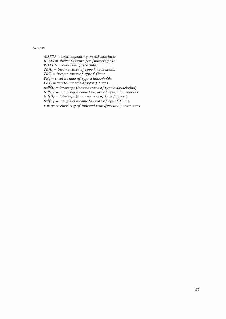
47

where: = = = = ℎℎ ℎ = = ℎℎ ℎ = ℎ0 = ( ℎℎ ℎ ) ℎ1 = ℎℎ ℎ 0 = ( ) 1 = =

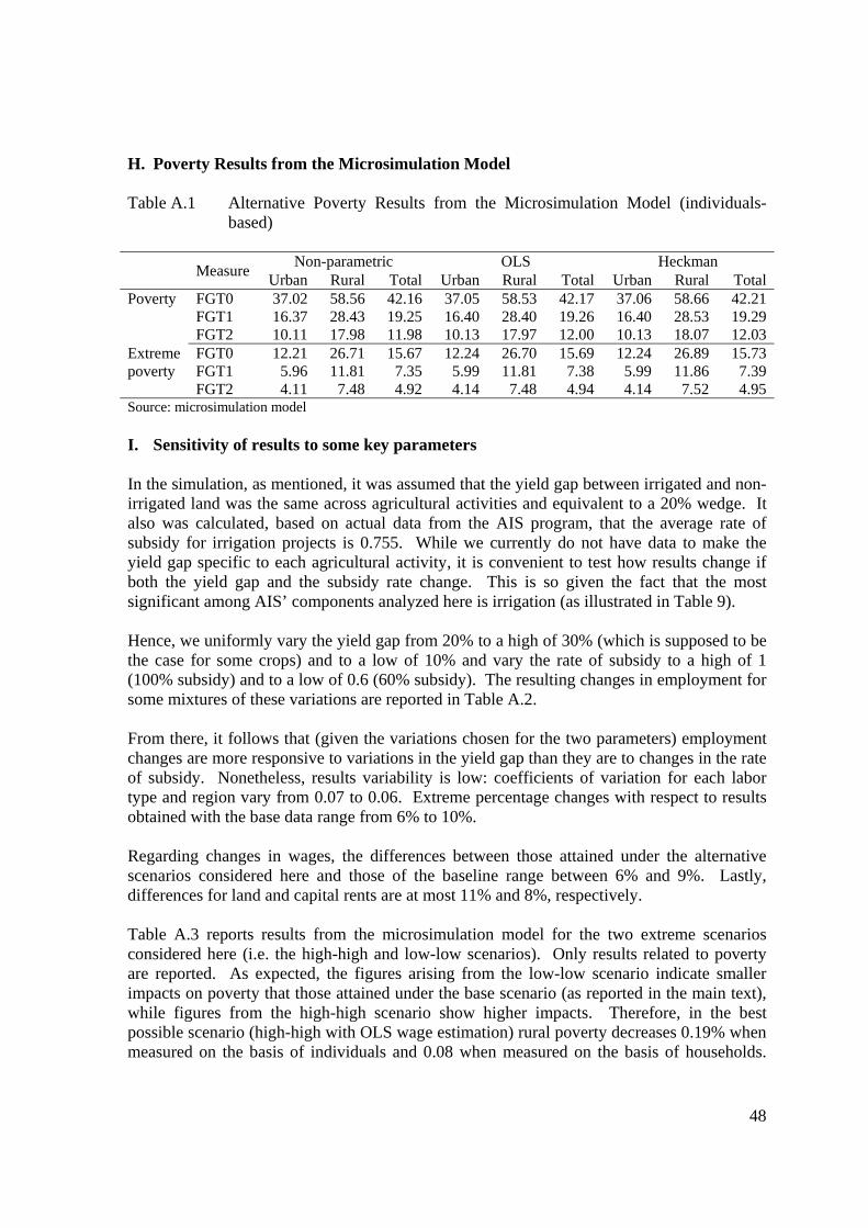
48

H. Poverty Results from the Microsimulation Model Table A.1 Alternative Poverty Results from the Microsimulation Model (individuals-

based)

Measure

Non-parametric OLS Heckman Urban Rural Total Urban Rural Total Urban Rural TotalPoverty FGT0 37.02 58.56 42.16 37.05 58.53 42.17 37.06 58.66 42.21

FGT1 16.37 28.43 19.25 16.40 28.40 19.26 16.40 28.53 19.29FGT2 10.11 17.98 11.98 10.13 17.97 12.00 10.13 18.07 12.03

Extreme poverty

FGT0 12.21 26.71 15.67 12.24 26.70 15.69 12.24 26.89 15.73FGT1 5.96 11.81 7.35 5.99 11.81 7.38 5.99 11.86 7.39FGT2 4.11 7.48 4.92 4.14 7.48 4.94 4.14 7.52 4.95

Source: microsimulation model I. Sensitivity of results to some key parameters In the simulation, as mentioned, it was assumed that the yield gap between irrigated and non-irrigated land was the same across agricultural activities and equivalent to a 20% wedge. It also was calculated, based on actual data from the AIS program, that the average rate of subsidy for irrigation projects is 0.755. While we currently do not have data to make the yield gap specific to each agricultural activity, it is convenient to test how results change if both the yield gap and the subsidy rate change. This is so given the fact that the most significant among AIS’ components analyzed here is irrigation (as illustrated in Table 9). Hence, we uniformly vary the yield gap from 20% to a high of 30% (which is supposed to be the case for some crops) and to a low of 10% and vary the rate of subsidy to a high of 1 (100% subsidy) and to a low of 0.6 (60% subsidy). The resulting changes in employment for some mixtures of these variations are reported in Table A.2. From there, it follows that (given the variations chosen for the two parameters) employment changes are more responsive to variations in the yield gap than they are to changes in the rate of subsidy. Nonetheless, results variability is low: coefficients of variation for each labor type and region vary from 0.07 to 0.06. Extreme percentage changes with respect to results obtained with the base data range from 6% to 10%. Regarding changes in wages, the differences between those attained under the alternative scenarios considered here and those of the baseline range between 6% and 9%. Lastly, differences for land and capital rents are at most 11% and 8%, respectively. Table A.3 reports results from the microsimulation model for the two extreme scenarios considered here (i.e. the high-high and low-low scenarios). Only results related to poverty are reported. As expected, the figures arising from the low-low scenario indicate smaller impacts on poverty that those attained under the base scenario (as reported in the main text), while figures from the high-high scenario show higher impacts. Therefore, in the best possible scenario (high-high with OLS wage estimation) rural poverty decreases 0.19% when measured on the basis of individuals and 0.08 when measured on the basis of households.

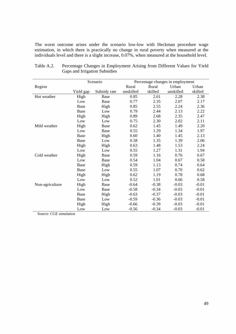
49

The worst outcome arises under the scenario low-low with Heckman procedure wage estimation, in which there is practically no change in rural poverty when measured at the individuals level and there is a slight increase, 0.07%, when measured at the household level. Table A.2. Percentage Changes in Employment Arising from Different Values for Yield

Gaps and Irrigation Subsidies

Region Scenario Percentage changes in employment

Yield gap Subsidy rate Rural

unskilled Rural skilled

Urban unskilled

Urban skilled

Hot weather High Base 0.85 2.61 2.28 2.38 Low Base 0.77 2.35 2.07 2.17 Base High 0.85 2.55 2.24 2.36 Base Low 0.79 2.44 2.13 2.22 High High 0.89 2.68 2.35 2.47 Low Low 0.75 2.30 2.02 2.11

Mild weather High Base 0.62 1.45 1.49 2.20 Low Base 0.55 1.29 1.34 1.97 Base High 0.60 1.40 1.45 2.13 Base Low 0.58 1.35 1.39 2.06 High High 0.63 1.48 1.53 2.24 Low Low 0.55 1.27 1.31 1.94

Cold weather High Base 0.59 1.16 0.76 0.67 Low Base 0.54 1.04 0.67 0.58 Base High 0.59 1.13 0.74 0.64 Base Low 0.55 1.07 0.70 0.62 High High 0.62 1.19 0.78 0.68 Low Low 0.52 1.01 0.66 0.58

Non-agriculture High Base -0.64 -0.38 -0.03 -0.01 Low Base -0.58 -0.34 -0.03 -0.01 Base High -0.63 -0.37 -0.03 -0.01 Base Low -0.59 -0.36 -0.03 -0.01 High High -0.66 -0.39 -0.03 -0.01 Low Low -0.56 -0.34 -0.03 -0.01

Source: CGE simulation

50

Table A.3 Poverty Results from the Microsimulation Model under the Alternative Values for Yield Gaps and Irrigation Subsidies

Non-parametric OLS Heckman Urban Rural Total Urban Rural Total Urban Rural Total

Scenario Low-Low; levels, individuals FGT0 37,082 58,579 42,207 37,112 58,548 42,222 37,125 58,697 42,268FGT1 16,376 28,406 19,244 16,404 28,379 19,259 16,405 28,521 19,294FGT2 10,111 17,968 11,984 10,139 17,951 12,001 10,139 18,056 12,026

Scenario Low-Low; levels, households FGT0 31,973 52,199 36,372 31,984 52,202 36,381 31,991 52,294 36,407FGT1 15,706 26,574 18,069 15,711 26,573 18,073 15,715 26,647 18,092FGT2 10,828 17,770 12,338 10,832 17,768 12,341 10,834 17,823 12,354

Scenario Low-Low; percentage changes, individuals FGT0 -0,031 -0,118 -0,052 -0,001 -0,149 -0,037 0,012 0,000 0,009FGT1 0,005 -0,191 -0,042 0,033 -0,218 -0,027 0,034 -0,076 0,008FGT2 0,014 -0,148 -0,025 0,042 -0,165 -0,008 0,042 -0,060 0,017

Scenario Low-Low; percentage changes, households FGT0 0,000 -0,022 0,003 0,020 -0,019 0,012 0,027 0,073 0,038FGT1 0,000 -0,093 -0,012 0,015 -0,094 -0,008 0,019 -0,020 0,011FGT2 0,000 -0,076 0,001 0,026 -0,078 0,004 0,028 -0,023 0,017

Scenario High-High; levels, individuals FGT0 37,035 58,545 42,163 37,066 58,510 42,179 37,071 58,637 42,213FGT1 16,370 28,444 19,249 16,400 28,422 19,266 16,401 28,541 19,295FGT2 10,105 17,998 11,987 10,135 17,983 12,006 10,135 18,074 12,028

Scenario High-High; levels, households FGT0 31,954 52,169 36,350 31,965 52,145 36,353 31,968 52,217 36,371FGT1 15,702 26,595 18,071 15,707 26,604 18,077 15,711 26,656 18,091FGT2 10,825 17,793 12,340 10,829 17,799 12,345 10,831 17,840 12,355

Scenario High-High; percentage changes, individuals FGT0 -0,078 -0,152 -0,096 -0,047 -0,187 -0,080 -0,042 -0,060 -0,046FGT1 -0,001 -0,153 -0,037 0,029 -0,175 -0,020 0,030 -0,056 0,009FGT2 0,008 -0,118 -0,022 0,038 -0,133 -0,003 0,038 -0,042 0,019

Scenario High-High; percentage changes, households FGT0 0,000 -0,052 -0,019 0,001 -0,076 -0,016 0,004 -0,004 0,002FGT1 0,000 -0,072 -0,010 0,011 -0,063 -0,004 0,015 -0,011 0,010FGT2 0,000 -0,053 0,003 0,023 -0,047 0,008 0,025 -0,006 0,018Source: microsimulation model