global poverty and distributional impacts of agricultural
TRANSCRIPT

Global Poverty and Distributional Impacts of
Agricultural Distortions
Maurizio Bussolo, Rafael De Hoyos and Denis Medvedev
World Bank, Washington DC
and
Mexico Under-Secretary of Education, Mexico City
Agricultural Distortions Working Paper 97, June 2009 This is a product of a research project on Distortions to Agricultural Incentives, under the leadership of Kym Anderson of the World Bank’s Development Research Group. The authors are grateful to Xiang Tao for research assistance; to Harry de Gorter, Alessandro Olper, and Gordon Rausser for many discussions and insights on this issue; to Kym Anderson for excellent collaboration and encouragement on the project; and to the World Bank for Trust Funds provided by the governments of the Netherlands (BNPP) and the United Kingdom (DfID). This paper will appear in Agricultural Price Distortions, Inequality and Poverty, edited by K. Anderson, J. Cockburn and W. Martin (forthcoming 2010). This is part of a Working Paper series (see www.worldbank.org/agdistortions) that is designed to promptly disseminate the findings of work in progress for comment before they are finalized. The views expressed are the authors’ alone and not necessarily those of the World Bank and its Executive Directors, nor the countries they represent, nor of the institutions providing funds for this research project.
Pub
lic D
iscl
osur
e A
utho
rized
Pub
lic D
iscl
osur
e A
utho
rized
Pub
lic D
iscl
osur
e A
utho
rized
Pub
lic D
iscl
osur
e A
utho
rized
Pub
lic D
iscl
osur
e A
utho
rized
Pub
lic D
iscl
osur
e A
utho
rized
Pub
lic D
iscl
osur
e A
utho
rized
Pub
lic D
iscl
osur
e A
utho
rized

Global Poverty and Distributional Impacts of
Agricultural Distortions
Maurizio Bussolo,a Rafael De Hoyosb and Denis Medvedevc
Abstract This paper assesses the potential impacts of the removal of agricultural and other trade
distortions using a newly developed dataset and methodological approach for evaluating the
global poverty and inequality effects of policy reforms. It finds that liberalization of
agriculture would increase global extreme poverty (US$1 a day) slightly and by almost 1
percent if other goods trade is also liberalized; but the number of people living on less than
$2 a day would fall by almost 1 percent. Beneath these small aggregate changes, most
countries witness a substantial reduction in poverty while South Asia – where half of the
world's poor reside – would experience an increase in extreme (but not moderate) poverty
incidence due to high rates of protection afforded to its unskilled labor-intensive agricultural
sectors. The distributional changes also are projected to be mild, but again exhibit a strong
regional pattern: inequality falls in Latin America, which is characterized by high initial
inequality, and rises in South Asia, has relatively low income inequality.
Keywords: Agricultural distortions, global poverty, income distribution, inequality
JEL classification: Q17, F17, D63, I32
a Senior Economist, Economic Policy Sector, Latin America and Caribbean Region, World Bank, Washington, DC, USA; [email protected] b Chief of Advisors, Under-Secretary of Education, Government of Mexico, Mexico City, Mexico; [email protected] c Economist, West Africa Poverty Reduction and Economic Management, World Bank, Washington, DC, USA; [email protected]

1
Global Poverty and Distributional Impacts of
Agricultural Distortions
Maurizio Bussolo, Rafael De Hoyos and Denis Medvedev
Trade liberalization is almost always welfare increasing nationally and globally, but it also
brings about large income redistributions. Simulation models calibrated on real world data
show that the aggregate gains for a country eliminating its tariffs are at best only a very few
percentage points of its initial GDP. Similarly, gains from multilateral trade policy reforms
for the whole world tend to be small. By contrast, losses suffered by specific, initially
protected, sectors or factors can be much larger. As Rodrik (1998) puts it, “the [static]
efficiency consequences of trade reform pale in comparison to its redistributive effects”.
These effects often create complicated policy challenges at both domestic and
international levels because, in most cases, losers tend to be a smaller and more vocal group
than winners.1 Perhaps the most recent and glaring example of this trade-related
distributional tension is the impasse of the Doha Round of the World Trade Organization
(WTO). Disputes over the reduction of agricultural market distortions have stalled the whole
multilateral trade negotiation process. The controversy is centered on the demands of
developing and agricultural-exporting countries for the phasing out of export subsidies and
domestic farm supports that are mainly in developed countries, in addition to the reduction of
import barriers.
This example illustrates that a distributional tension between countries can have
important implications for international relations and global welfare. An additional question
is: would resolving trade disputes improve the distribution of income not only between
countries but also within national economies? The answer depends in part on own-country
distortions to agricultural and other producer incentives in individual developing countries.
1 According to Anderson and Martin (2005), self-interested vocal groups lobbying hard for excluding agricultural liberalization from multilateral negotiations include “not just farmers in the highly protecting countries and net food importing developing countries but also those food exporters receiving preferential access to those markets including holders of tariff rate quotas, members of regional trading agreements, and parties to non-reciprocal preference agreements including all least-developed countries.”

2
Often those policies privilege urban dwellers by protecting their industries and maintaining
low prices for food items to the disadvantage of often-poorer local farmers, although much
less so now than in the 1960s and 1970s (Krueger, Schiff and Valdes 1988, Anderson 2009).
Given that poverty is highest among farmers (Chen and Ravallion 2007), the poverty
reduction potential of agricultural trade liberalization is promising.
Using an ex-ante simulation analysis, this chapter answers the following questions: how
much would global inequality and poverty be reduced if all distortions to trade in agricultural
and other goods were removed? How much of that change would be due to just agricultural
policy reform? What share of the change in inequality would be due to changes between
countries versus within countries (bearing in mind that a lowering of inequality between
agricultural and non-agricultural groups could be offset by, for example, increased inequality
within the agricultural sector)? What would happen to global poverty, and to the incidence of
poverty in specific countries and regions? Does it matter whether we use the 1 dollar or 2
dollar a day international poverty line (because, for example, more non-agricultural
households than farm households may be clustered between those two poverty lines)?
The empirical results of this study are produced using the World Bank’s LINKAGE
global general equilibrium model (van der Mensbrugghe 2005) and the newly developed
Global Income Distribution Dynamics (GIDD) tool (Bussolo, De Hoyos and Medvedev
2008). GIDD is a framework for ex-ante analyses of the income distributional and poverty
effects of changes in macroeconomic, trade and sectoral policies and/or trends in global
markets. It complements a global CGE analysis by providing global micro-simulations based
on standardized household surveys. The tool pools most of the currently available household
surveys covering 1.2 million households in 73 developing countries. Household information
from developed countries completes the dataset. Overall, the GIDD sample covers more than
90 percent of the world’s population.2
The chapter is organized as follows. The next section presents the GIDD datasets and the
main features of the global income distribution, as a way of establishing the initial conditions
or baseline. This descriptive analysis sets the stage for the following sections which illustrate
the modeling methodology, lay out the reform scenarios, and summarize the main results.
The two core simulations involve liberalizing all merchandise trade and agricultural domestic
distortions, and – so as to see the contribution of farm and food policies – liberalizing just
2 The GIDD dataset, methodology and applications are available from: www.worldbank.org/prospects/gidd

3
agricultural trade and domestic price-distorting measures. Some final remarks are provided in
the concluding section.
What is at stake? The initial conditions
Almost 45 percent of the world’s people – most of them in developing countries – live in
households where agricultural activities represent the main occupation of the head. A large
share of this agriculture-dependent group, close to 32 percent, is poor. Agricultural
households thus contribute disproportionably to global poverty: three out of every four poor
people belong to this group. Thus changing economic opportunities in agriculture can
significantly affect global poverty and inequality. The specific opportunity considered in this
study is the removal of agricultural subsidies and taxes and all merchandise trade distortions.
Direct effects of this global liberalization will be changes in the international prices of food
and other agricultural products and in the returns of factors used intensively in agriculture,
with these changes determining winners and losers through their impacts on different
households’ earnings and spending.
Before considering these effects in detail, this section describes what is at stake by
considering the socio-economic characteristics of the world’s population, especially those
engaged in agriculture. This initial descriptive analysis is based on the GIDD dataset that has
been recently developed at the World Bank. The GIDD dataset consists of 73 detailed
household surveys for low- and middle-income countries, complemented with more
aggregate information on income distribution for 25 high-income and 22 other developing
countries.3 Together, data on these 120 countries cover more than 90 percent of the global
population. Country coverage varies by region: while the GIDD dataset includes more than
97 percent of population in East Asia, South Asia, Latin America, and Eastern Europe and
Central Asia,, its coverage in Sub-Saharan Africa and in the Middle East and North Africa is
limited to 76 and 58 percent of population, respectively. Among the detailed surveys, the
majority (54) use per capita consumption as the welfare indicator, while the remaining
surveys—all but one for countries in Latin America—include only per capita income as a 3 This more aggregate information usually consists of 20 data points for each country, with each data point representing the average per capita income (or consumption) of 5 percent of the country’s population. In the absence of full survey data, using these “vintile” data provides a close approximation to most economy-wide measures of inequality.

4
measure of household welfare. Both income and consumption data are monthly; the data are
standardized to the year 2000 and are expressed in 1993 PPP prices for consistency with the 1
and 2 dollar a day poverty lines, which are calculated at 1993 PPP exchange rates.4
Three facts about the agricultural sector help determine the welfare effects of a global-
scale removal of trade distortions: the proportion of the world’s people whose real incomes
depend on the agricultural sector; the initial position of the agricultural population in the
global income distribution; and the dispersion of incomes among the agricultural population.
Using the GIDD dataset, figure 1 shows a kernel density for the global income
distribution of household per capita income/consumption and kernel densities for
income/consumption of the population in and out of the agricultural sector, respectively.5 The
area below the kernel density for the agricultural sector is equal to 0.45, indicating that 45
percent of the world population relies on agriculture for its livelihood. The distribution of the
agricultural population is located to the left of the non-agricultural distribution, implying that
households in the agricultural sector earn, on average, lower incomes than their counterparts
in other sectors. In Purchasing Power Parity (PPP) US dollars, the average agricultural
household’s per capita monthly income is $65, just 20 percent of the $320 per capita income
earned by the average households in the non-agriculture group. The differences in shape
between the two distributions corroborates what Kuznets hypothesized more than 50 years
ago, which is that incomes in the traditional sector are less dispersed than in the modern
sectors. A more egalitarian traditional sector is depicted in the form of a taller and thinner
distribution for agricultural population in figure 1.
Income inequality can be estimated from the global income distribution data depicted in
figure 1. The Gini index for the world is equal to 0.67, which denotes a high level of
inequality. In fact, the global Gini is about 28 points worse than that of the United Sates and
even higher than the level observed in extremely unequal countries such as Mexico. As
Bourguignon et al. (2004) note: “if the world were a country, it would be among the most
unequal countries of the world.” How much of this inequality can be explained by the 4 The adjustment procedure for expressing welfare indicators in 1993 international dollars (PPP) is as follows. First, for countries with a survey year different from 2000, the welfare indicator (household per capita income or consumption) is scaled to the year 2000 using the cumulative growth in real income per capita between the survey year and 2000. Then, the welfare indicator is converted to 1993 national prices by multiplying the welfare indicator by the ratio of CPI in 1993 to the CPI in the survey year. Finally, the welfare indicator is converted to 1993 international prices by multiplying the outcome of the previous calculations by the 1993 PPP exchange rate. 5 The distributions for the agricultural and non-agricultural populations are not, strictly speaking, density functions since the area below the curve does not add to 1. The densities of the agricultural and non-agricultural population had been rescaled so that the area under the curve represents the proportion of the world’s population within these two groups.

5
disparity on average incomes between the agricultural group and the rest? Inequality
decomposition analysis shows that one-quarter of global income disparities can be explained
by the difference in average incomes between the two groups of households, the remaining
three-quarters are due to within-group income variation.
Based on the pre-established poverty line of 1 dollar (PPP) per day, the GIDD global
income data also provide information about the differences in poverty incidence among the
two population subgroups. Despite the fact that incomes are better distributed among the
agricultural population (the Gini coefficient is 18 points lower in agriculture than in non-
agriculture), lower average incomes in this sector result in a much higher poverty incidence:
32 percent of agricultural households are poor compared with 8 percent of non-agricultural
households.
In terms of personal characteristics of the poor in and out of the agricultural sector, no
noticeable differences are observed in the average age of the head or in the household size.
However, poor people in agriculture tend to have lower education levels: only 32 percent of
them has completed primary education, compared with 46 percent for non-farm households.
In agriculture, poor households headed by a woman are a small minority, less than 9 percent,
which is significantly below the 14 percent observed for non-agricultural households (table
1).
Up to this point the welfare information on agricultural and non-agricultural populations
has been derived by agglomerating all households within these two groups irrespective of
their nationality. In fact, the kernel densities in figure 1 exploit full income heterogeneity
across households, including variations between and within countries. Countries display large
differences in terms of their population size, their level of development, and the importance
of the agricultural sector in their economies. These three country-specific characteristics are
important determinants of prospective change of global poverty and global inequality. As can
be seem from figure 2, global poverty would be strongly reduced if China and India were to
move to higher income levels. Given their initial large share of the global population and
their position in the global income distribution, the economic expansion of these two giants is
a key factor shaping the evolution of the world economy.6 Figure 2 also depicts a negative
relationship between income levels and share of workers in agriculture, and although this
relationship is imperfectly inferred from a cross-section of countries at a particular point in
time, it suggests that structural shifts will likely affect income distribution within countries. 6 For a specific analysis of the importance of China and India for global growth and income distribution, see Bussolo et al. (2007).
6
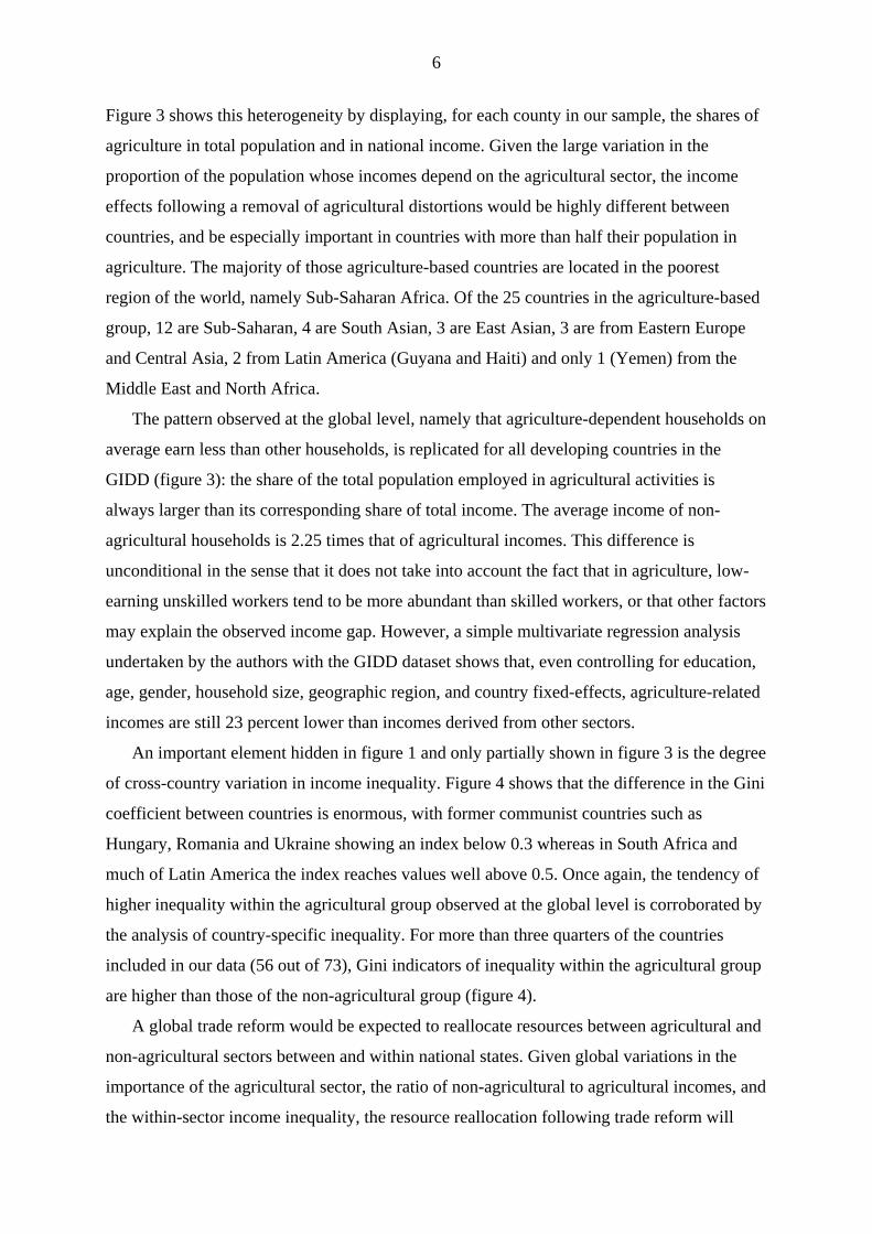
Figure 3 shows this heterogeneity by displaying, for each county in our sample, the shares of
agriculture in total population and in national income. Given the large variation in the
proportion of the population whose incomes depend on the agricultural sector, the income
effects following a removal of agricultural distortions would be highly different between
countries, and be especially important in countries with more than half their population in
agriculture. The majority of those agriculture-based countries are located in the poorest
region of the world, namely Sub-Saharan Africa. Of the 25 countries in the agriculture-based
group, 12 are Sub-Saharan, 4 are South Asian, 3 are East Asian, 3 are from Eastern Europe
and Central Asia, 2 from Latin America (Guyana and Haiti) and only 1 (Yemen) from the
Middle East and North Africa.
The pattern observed at the global level, namely that agriculture-dependent households on
average earn less than other households, is replicated for all developing countries in the
GIDD (figure 3): the share of the total population employed in agricultural activities is
always larger than its corresponding share of total income. The average income of non-
agricultural households is 2.25 times that of agricultural incomes. This difference is
unconditional in the sense that it does not take into account the fact that in agriculture, low-
earning unskilled workers tend to be more abundant than skilled workers, or that other factors
may explain the observed income gap. However, a simple multivariate regression analysis
undertaken by the authors with the GIDD dataset shows that, even controlling for education,
age, gender, household size, geographic region, and country fixed-effects, agriculture-related
incomes are still 23 percent lower than incomes derived from other sectors.
An important element hidden in figure 1 and only partially shown in figure 3 is the degree
of cross-country variation in income inequality. Figure 4 shows that the difference in the Gini
coefficient between countries is enormous, with former communist countries such as
Hungary, Romania and Ukraine showing an index below 0.3 whereas in South Africa and
much of Latin America the index reaches values well above 0.5. Once again, the tendency of
higher inequality within the agricultural group observed at the global level is corroborated by
the analysis of country-specific inequality. For more than three quarters of the countries
included in our data (56 out of 73), Gini indicators of inequality within the agricultural group
are higher than those of the non-agricultural group (figure 4).
A global trade reform would be expected to reallocate resources between agricultural and
non-agricultural sectors between and within national states. Given global variations in the
importance of the agricultural sector, the ratio of non-agricultural to agricultural incomes, and
the within-sector income inequality, the resource reallocation following trade reform will

7
have significant distributional effects both between and within countries. Can economic
theory provide some guidance on the expected global welfare effects following the removal
of agricultural and other trade distortions?
As shown in Winters (2002) and McCulloch, Winters and Cirera (2001), trade
liberalization and household welfare are linked via prices, factor markets, and consumer
preferences. International prices of many agricultural products would increase with the
removal of trade barriers (Anderson and Martin 2005; Anderson, Valenzuela and van der
Mensbrugghe 2010). Assuming some degree of pass-through, the increase in international
prices would be followed by a rise in domestic agricultural prices, encouraging a
redistribution of resources from non-agricultural activities to the agricultural sector of the
economy. Based on figure 1, such redistribution could help reduce global poverty and
inequality. However, household consumption patterns will also change as a result of the shift
in prices, making the link between trade liberalization and global household welfare more
complex. As a consequence of the agricultural price changes, a redistribution of real income
will take place between net sellers and net buyers of agricultural products, with the welfare of
the former improving at the expense of the latter.7 Finally, factor prices will also change after
trade liberalization, thus changing real incomes of households that are not directly involved in
agricultural production.
The transition from trade theory to real world analysis presents serious challenges. A
sound empirical strategy has to estimate the effects of the reform on prices, monetary
incomes (via profits in the case of farm households and returns to factors of production for
non-farm households), consumption, and transfers.8 The framework used in this chapter, and
described in more detail below, accounts for the impact of trade liberalization through at least
some of these channels.
Methodology
7 A household is defined as a net producer (consumer) of agricultural products when the monetary income it derives from merchandising these products is greater (smaller) than the amount spent on them. 8 For empirical applications of trade’s effect on household welfare that take into account these effects, see for example the Mexican case studies by Nicita (2004) and De Hoyos (2007).

8
The empirical analysis in this paper relies on the GIDD database, a newly developed tool for
analyzing Global Income Distribution Dynamics.9 The GIDD, developed at the Development
Prospects Group of the World Bank, combines a consistent set of price and volume changes
from a global CGE model with micro data at the household level to create a hypothetical or
counterfactual income distribution capturing the welfare effects of the policy under
evaluation.10 Therefore, the GIDD has the ability to map CGE-consistent macroeconomic
outcomes to disaggregated household survey data.
The GIDD’s framework is based on micro-simulation methodologies developed in the
recent literature, including Bourguignon and da Silva (2003), Ferreira and Leite (2003, 2004),
Chen and Ravallion (2003), and Bussolo, Lay and van der Mensbrugghe (2005). The starting
point is the global income distribution in 2000, assembled using data from household surveys
(see above).11 The hypothetical distribution is then obtained by applying three main
exogenous changes to the initial distribution: changes in relative wages across skills and
sectors for each country, changes in household purchasing power due to shifts in food and
other prices, and changes in the average level of welfare (real income) for each country.
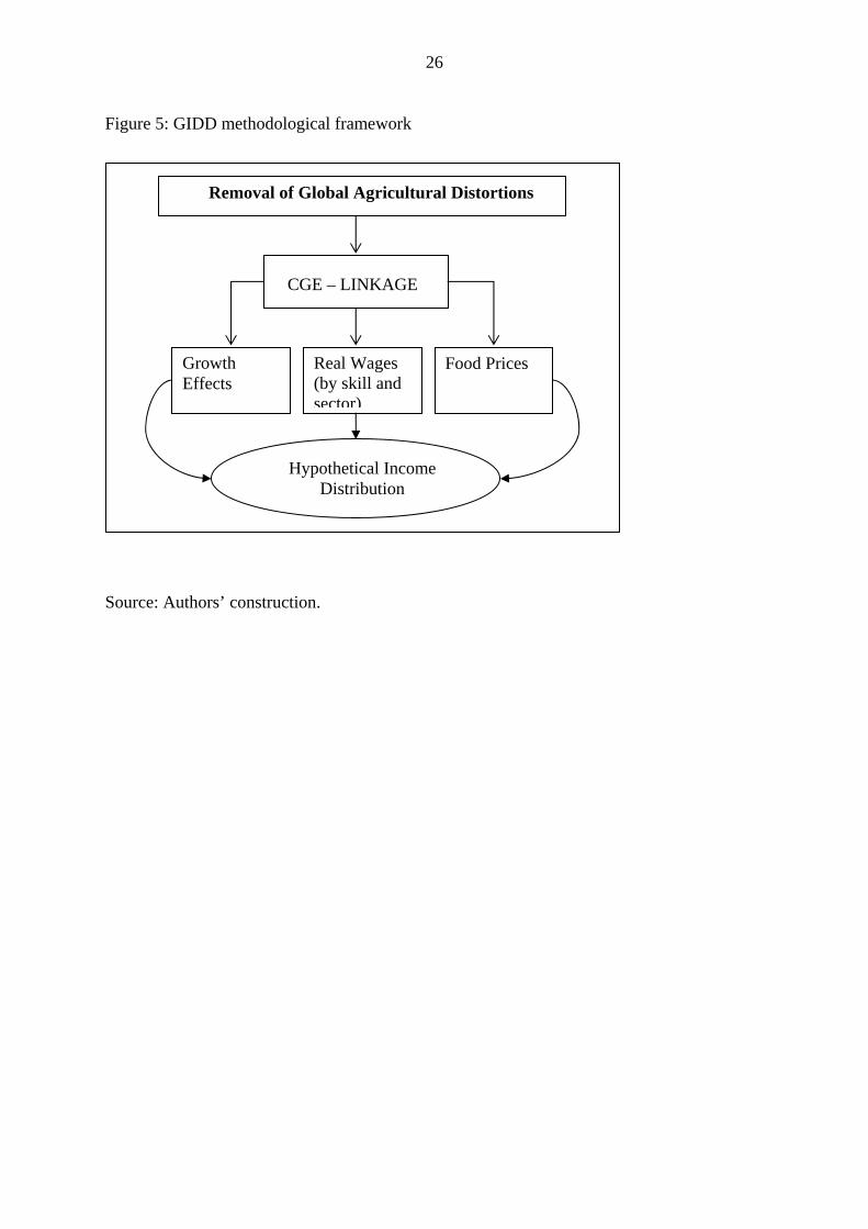
The methodological framework used here is depicted in figure 5. The starting point is the
price and quantity effects following the removal of trade distortions, which are computed
using the global CGE Linkage model (top part of figure 5). The CGE model will compute the
values of the three variables linking the macro and micro levels of the model (middle part of
figure 5): overall economic growth, real wage premiums among agricultural/non-agricultural
and skilled/unskilled groups, and the consumption (or real income) effects brought about by
the change in the relative price of food. These CGE results are passed on to the household
survey data, creating a new, hypothetical household income distribution (bottom part of
figure 5). This is accomplished by differentiating four types of households: those where the
household head is an (1) unskilled agricultural worker, (2) skilled agricultural worker, (3)
unskilled non-agricultural worker, or (4) skilled non-agricultural worker. The initial income
premium earned by groups (2)-(4) relative to group (1) is changed in accordance with
changes in the wage premiums in the CGE model, which uses the GIDD's information on a
number of workers in each of the segments (1)-(4). For example, if initially an unskilled-
headed household in non-agriculture earns 50 percent more than an unskilled-headed
9 A detailed methodological description of the GIDD can be found in Bussolo, De Hoyos and Medvedev (2008). 10 The GIDD uses the LINKAGE model as the global CGE framework. See van der Mensbrugghe (2005) for a detailed description of LINKAGE. 11 Throughout this chapter, when we talk about the global distribution we are referring to the GIDD’s sample, which covers 92 percent of the world’s population.

9
household in agriculture, and the CGE results show that this premium would reduce by one-
tenth, the micro-simulation part of the GIDD changes the incomes of all unskilled-headed
households in non-agriculture such that the new wage premium is 45 percent. In addition to
these wage shocks, the GIDD also accounts for changes in relative prices and changes in per
capita income, therefore indirectly picking up the impact on returns to factors other than
labor.
In the real world the changes depicted in figure 5 take place simultaneously, but in the
GIDD’s simplified framework they are accommodated in a sequential fashion. In the first
step, changes in labor remuneration by skill level and sectoral location are applied to each
household in the sample, depending on their education and sector of employment. In the
second step, consistent with an overall growth rate of real income per capita, real household
incomes are affected by the change in the price of food versus non-food: households with a
higher share of household income allocated to food consumption will bear a larger
proportional impact after a change in the price of food.
Comparisons between the initial and the counterfactual income distributions will capture
the welfare and inequality effects of the removal of global trade distortions. By taking into
account labor market effects (returns to skills in the agricultural sector and in the rest of the
economy) and consumption effects, GIDD’s framework closely maps the theoretical linkages
outlined in the previous section.12 However, the framework reshapes national income
distributions under a set of strong assumptions. In particular, income inequality within
population subgroups, formed by skills and sector of employment, is assumed to remain
constant after the trade reform. Moreover, data limitations affect estimates of the initial
inequality and its evolution. Although consumption expenditure is a more reliable welfare
measure than income, and its distribution is normally more equal than the distribution of
income, consumption data are not available for all countries’ surveys. To get a global picture,
the present study had to include countries for which only income data were available along
with countries with consumption information. Finally, measurement errors implicit in
purchasing power parity exchange rates, which have been used to convert local currency
units, also affect comparability across countries. The resulting hypothetical income
distribution should thus not be seen as a forecast of what the future distribution might look
like; rather, it should be interpreted as the result of an exercise that captures the distributional
effect of trade liberalization, ceteris paribus. 12 The GIDD does not take into account the welfare impacts via any changes in remittances/ transfers between households resulting from trade reform.

10
What happens to poverty and income distribution when trade is liberalized globally?
In this section, we link the macro outcomes of global agricultural and other trade policy
reforms to the changes in the distribution of income between and within countries. Our
analysis is carried out in three stages. First, we briefly examine the macroeconomic results
from the LINKAGE model simulations of global trade reform similar to those presented in
the previous chapter (Anderson, Valenzuela and van der Mensbrugghe 2010),13 focusing on
the variables that are passed on to the household survey data. Second, we consider the income
distributional results from a global perspective, quantifying the likely changes in global
poverty and inequality and identifying groups of countries and individuals that are likely to
benefit the most (least) from global trade reform. Third, we assess the potential trends in the
distribution of income within countries, identifying countries where inequality and poverty
pressures may heighten and thus erode support for additional reforms.
Macroeconomic general equilibrium results
The LINKAGE simulation analysis has been carried out with version 7.0 of the GTAP
database, amended by Valenzuela and Anderson (2008) to take account of new estimates of
distortions to agricultural incentives in developing countries (compiled by Anderson and
Valenzuela 2008). The LINKAGE model disaggregates global trade into bilateral flows
between more than 100 countries/regions in 57 commodity groups. The base year for the
simulations is 2004, and the baseline data have taken into account changes in the global trade
and tariff structure due to the implementation of the Uruguay Round commitments, EU
enlargement, China’s accession to the WTO, and implementation of most major preferential
trade agreements in place at that time. The model is solved in a comparative static mode,
which means that simulations are implemented as one-time shocks and do not take into 13 The Linkage results used here are not identical to those in the previous chapter because labour mobility in this chapter has been restricted to better match up with the available micro data. In the version of Linkage used in the previous chapter, the assumption of full factor mobility leads to an equalization of factor prices across sectors. However, the household survey data shows large and persistent differences between labour earnings in agriculture and non-agriculture, controlling for other relevant characteristics. Imposing the equalization of wages in the GIDD would lead to large and implausible changes in the distribution of income; therefore, in order to maintain consistency between macro and micro models, labour mobility in the macro model was limited.

11
account potential growth effects through changes in capital accumulation rates or variations
in productivity.
Our two simulations envision the full removal globally of trade taxes and subsidies on all
agricultural goods and lightly processed food without, and with, trade reform of non-
agricultural goods. With these two scenarios we are able to see the relative contribution to
changes in the global economy following the removal of just agricultural distortions.
The removal of distortions to trade in agricultural products causes global consumption to
rise by 0.29 percent, or two-thirds of the improvement expected under a trade liberalization
scenario involving all goods. Developing countries gain more than the average, with their
consumption rising by 0.47 percent compared to 0.24 percent for high-income countries. No
less than 50 out of 60 LINKAGE country/regions—representing nearly 95 percent of the
world’s people—experience positive changes in consumption following the removal of
agricultural distortions, compared to 47 country/regions that enjoy consumption gains from
liberalizing all goods trade (figure 6).
There are three main channels that transmit the trade reform shocks to household
consumption in the LINKAGE model and help explain the heterogeneity of the results in
figure 6. The first channel is the changes in the terms of trade, the ratio of export prices to
import prices without taking into account domestic price distortions caused by own-country
policies. Net exporters of agriculture and food, such as Brazil, Ecuador and New Zealand,
reap significant welfare gains when their export prices of farm commodities rise by an
average of 8, 19, and 11 percent, respectively.14 On the other hand, net importers of food,
such as China, Mexico and Senegal, experience real consumption losses due to higher import
prices.
The second channel is tightly linked to the first, and has to do with the impact of own-
country policies. Thus, countries with high pre-reform tariffs or export taxes, such as
Lithuania, Nigeria and the group in North Africa, tend to experience larger consumption
gains than countries where the initial distortions are low. If the initial agricultural import
barriers are sufficiently high, consumers may face lower post-reform prices of food even if
import prices are rising. This is the case in North Africa, which experiences an increase in
real consumption despite being a net food importer.
14 The price increases are calculated using the Paasche price index, i.e. using the post-reform exports as weights for aggregating the prices of individual commodities. Unless explicitly noted, all price indices in this section are calculated using the Paasche formula. Price indices differ by country due to differences in the composition of exports (i.e., aggregation weights).

12
The third channel is the impact of trade reform on government budgets. Since the model
does not include an explicit transversality condition, we maintain a fixed budget deficit
closure, which means that any losses in public revenue (such as a reduction in tariff income)
must be offset by a compensatory increase in the direct tax rate on households.15 Therefore,
welfare gains are more limited in countries such as Tanzania and Zimbabwe, which rely
heavily on international trade taxes as an important provider of public revenue.16
In addition to changes in levels of per capita consumption across countries, the
LINKAGE results hint at important distributional consequences of trade reform within
countries, which come about through changes in returns to labor in different sectors and at
varying skill levels. Figure 7 shows the contributions of payments to different factors to the
total change in real GDP at factor cost (in percentage points) following the removal of just
agricultural distortions. With the exception of China, all those countries experiencing an
increase in payments to unskilled labor in agriculture also register consumption gains due to
agricultural policy reform. However, the converse does not hold: real consumption increases
in 32 out of 41 countries that show a decline in unskilled agricultural wages. Since unskilled
workers in agriculture tend to be the poorest part of the population, these results suggest that
pressures towards increased inequality may intensify.17 Furthermore, the losses and gains in
agricultural wages exhibit strong regional patterns: real wages of unskilled farmers rise in
Latin America, the Middle East and East Asia, while declining in other developing regions,
and, much more strongly, in high-income countries.
The initial level of protection in agriculture, combined with the terms of trade shock,
represent the main determinants of the trends in farm factor prices. Consider the example of
India, where unskilled farm wages decline by 6.1 percent following trade reform.18 Indian
farmers must contend with falling international prices of imported farm products (a decline of
1.7 percent) as well as a loss of tariff protection (2.0 percent), export subsidies (3.3 percent),
and output subsidies (6.9 percent) if all farm policies are scrapped. The first two channels
decrease the farmers’ competitiveness on the domestic market and lead to higher import 15 In other words, this closure choice gives rise to consistent measurement of household utility, as the utility function does not include the consumption of public goods. 16 In this situation, the ability of households to gain or lose from trade reform depends on (in addition to the impacts of the first two channels) their ability to substitute out of more expensive goods into now-cheaper alternatives. 17 Note that trends in consumption per capita are unlikely to be representative of the welfare of agricultural households, since their weight in total consumption is low due to limited incomes and a high incidence of poverty. 18 The 6.1 percent figure refers to the decline in the nominal wages. The change in real wages depends on the choice of deflator: while the consumer price index increases by 2 percent relative to the base year, the GDP deflator falls by 1 percent.

13
penetration, the third channel erodes their competitiveness on the international markets, and
the fourth channel increases production costs and makes Indian farmers less competitive
overall. Together, these effects result in a strong negative shock to farm labor earnings.
In Mexico, the income losses among unskilled farmers are lower than in India. This is
partially attributable to its close trading relationship with the United States. Mexico purchases
75 percent of its agricultural imports from the US, whose export prices rise by 5.7 percent
due to the elimination of export and production subsidies. Thus, the removal of agricultural
price supports in the US puts upward pressure on import prices of farm products in Mexico,
which hurts consumers but increases the competitiveness of Mexican farmers on the domestic
market. On the other hand, this trend is counteracted by the removal of Mexico’s tariff
protection on agriculture (1.2 percent) and its farm output subsidies (0.8 percent), which lead
to a decrease in competitiveness of farmers in Mexico and market share losses for them in
both domestic and export markets.
Brazil, by contrast, is an example of a country where a number of positive developments
combine to produce a nearly 34 percent gain in the wages of unskilled agricultural workers.19
The import prices of farm products in Brazil rise by 1.8 percent, bolstering the domestic
competitiveness of its farmers, while export prices increase by more than 10 percent. Because
Brazilian farmers do not receive export or production subsidies, they are well-positioned to
take advantage of these opportunities and gain market share both domestically and abroad.
Although some of the gains to agricultural producers are offset by the loss in domestic
protection (import tariff of 2.4 percent), Brazilian agriculture is still able to increase its
production volume by 18 percent following farm trade reform.
Micro-simulation results: a first look at global poverty and inequality effects
In this section, we use the GIDD model and data to simulate the likely changes in global
poverty and inequality due to the elimination of trade distortions. Given the richness of the
data and the numerous factors affecting global poverty and inequality within the GIDD, this
section starts with two simulations that illustrate, in a simple way, the expected effects of a
global trade policy reform. Focusing only on developing countries in our dataset, both
simulations raise the average income in the developing world by 1 percent. In the first
simulation, national income increases due to an increase in incomes of agricultural
19 This is a nominal, not a real increase. Consumer prices in Brazil rise by 4 percent following trade reform.

14
households only, while in the second simulation the increase is due entirely to an expansion
in non-agricultural incomes. The results of these examples are shown with two growth
incidence curves (GIC)20 in figure 8. The thin GIC captures the effects of assigning income
gains only to agricultural households, while the thick GIC raises incomes only for those
households whose head works in non-agricultural activities.
As expected, the increase in agricultural incomes is more pro-poor than the same income
change taking place in other sectors where households are relatively richer. This pro-poor
bias of growth in agricultural incomes is reflected in the downward slope of the thin GIC,
with the poorest households reaping the largest income gains. A different way of interpreting
the results of figure 8 is to observe that, if agricultural sectors in all developing countries
receive income gains above those in the non-agricultural sectors as a result of the elimination
of distortions, global poverty and inequality would fall. As shown in the discussion below,
the reality tends to be much more complex than these simple simulations, but nonetheless the
central message of figure 8 captures the essence of the GIDD simulations.
Global poverty and inequality impacts
Translating the shocks from the LINKAGE model into poverty and inequality outcomes with
the GIDD shows that the effects of a full removal of agricultural price and trade distortions
on extreme poverty globally are close to zero (column 3 of table 2). This limited impact is
explained by several factors. First, the impacts come from a comparative static rather than a
dynamic model, and so they do not capture the growth effects of the reform. Thus the
changes in per capita consumption are very small, arising just from the income boost from
more-efficient resource allocation. According to the GIDD, the world’s average monthly
household income increases 0.3 percent after the removal of just agricultural distortions,
passing from an initial level of $204 to a final value of $210 in 1993 PPP. Even when
nonagricultural trade is also liberalized, global income increases only slightly more but the
number of households living on less than $1 a day still remains the same in total.
Second, there is an income redistribution from farm to nonfarm households, so that the
incidence of extreme poverty among farm households rises by around 1 percent in both
scenarios while its incidence among nonfarm households falls by 0.2 or 0.3 percent. As a
20 The GIC shows the changes in welfare along the entire income distribution, therefore capturing, in a single graph, the growth and distributional components of overall welfare changes. For a detailed description of the properties characterizing growth incidence curves, see Ravallion and Chen (2003).

15
result, the share of extremely poor households that are farmers rises from 76 to 77 percent
(columns 3 and 4 of table 1)
Third, the definition of poverty matters. The extreme level of less than $1 a day suggests
only 8 percent of nonfarm households are poor and that they account for just one in four poor
households, whereas that share is 27 percent and they account for nearly one in three poor
households at the moderate poverty definition of less than $2 a day. When we use that
moderate definition of poverty, we find that both agricultural and all merchandise trade
liberalization globally lower the poverty incidence by nearly 1 percent in total, and they
reduce it for farm as well as non-farm households (compare columns 3 and 5 of table 2).
The policy reforms also have only a slight impact in reducing income inequality at the
overall global level. Incomes rise in both the agricultural and non-agricultural sectors, and
agricultural incomes increase by twice as much in the all-goods reform scenario and by five
times as much in the agriculture-only reform (1.1 percent compared just 0.2 percent – see
column 2 of table 2). Yet while that reduction in the non-agricultural income premium on its
own reduces inequality, income dispersion within the agricultural sector also increases such
that the final change in global income distribution is close to zero, according to the Gini
coefficient changes in column 1 of table 2.
It is because of these distributional changes taking place within the agricultural sector that
the incidence of extreme poverty (under $1 a day, PPP) in this sector rises. It increases by 0.9
percentage points as a consequence of the elimination of agricultural price and trade
distortions, and by 1.1 points when nonfarm trade policies also are reformed. At the same
time, poverty among non-agricultural households experiences a reduction equal to 0.3 or 0.2
percentage points. The combination of poverty changes occurring in and out of the
agricultural sector ends up increasing extreme poverty by 0.2 percentage points from
agricultural-only reform, and by 0.4 points when all goods markets are freed, the latter
pushing 9 million additional individuals below the extreme poverty line of $1 a day. Bear in
mind, though, that the poverty effect of those reforms depends on where the poverty line is
set. While the global number of people in poverty measured by the $1 a day poverty line
shows an increase of 1.0 percent as a consequence of all-goods reform, the number when
measured using the $2 a day criterion actually falls, by about 20 million or 0.8 percent
(columns 4 and 5 of table 3).
The above results have treated the world as a single entity, making no distinction between
regions or countries. Lack of major changes at the global level can be the outcome of
offsetting impacts across regions. As discussed above, farmers in Latin America are big

16
winners from agricultural price and trade reform, with an impressive increase of 16 percent in
their household income. By contrast, incomes of farmers in South Asia would shrink more
than 3 percent if agricultural distortions are dismantled globally. In order to show the
incidence of these changes among the population in the different regions, figure 9(a) plots the
GIC for Latin America, South Asia and the rest of the world. The GIC for Latin America
shows that agriculture-based growth in the region is highly pro-poor. By contrast, agriculture-
based growth in South Asia is highly regressive, with the poorest households losing from
such reform. East Asia and, to a lesser extent, Sub-Saharan Africa would benefit from global
agricultural reform, and the effects of such reform would be progressive, albeit small, for the
rest of the world.
The differences in reform outcomes across regions help explain the lack of significant
change in global poverty. With nearly half a billion of its people in extreme poverty and
another 625 million moderately poor, South Asia alone accounts for about half of global
poverty, while Latin America accounts for less than 5 percent (column 1 of table 3). Hence,
although removing agricultural distortions alleviates extreme poverty in most regions in the
world, the increase in South Asia’s headcount ratio slightly more than offsets these gains.
The results using the $2 a day poverty line show a more positive picture. Poverty by that
standard is alleviated in all key regions except (very marginally) for Sub-Saharan Africa
(final column of table 3). The results at the moderate poverty line are particularly interesting
for South Asia, where agricultural reform becomes pro-poor, instead of anti-poor as it was
when using the $1 a day extreme poverty line. This result is explained by the large number of
non-agricultural households that are between the two poverty lines in South Asia, who would
experience an increase in purchasing power if global agricultural markets were liberalized.
The reduction in moderate poverty is somewhat less when nonfarm goods trade also is
liberalized, but is still 0.8 percent or 20 million people globally.
Poverty and inequality effects within regions and countries
Global agricultural liberalization has distributional and poverty effects that vary not only
across regions but also between neighboring countries and within countries. This section
summarizes the poverty effects for each of the countries included in our sample and the
distributional changes taking place within them. Table 3 shows that the 5 million individuals
that would be pushed into poverty as a consequence of agricultural reform is the combination
of a 15 million increase in poverty in South Asia and a 10 million decrease in poverty in all
other regions. Figure 10 shows the specific countries that contribute the most to this reduction

17
and increase in global poverty, respectively. On the one hand, among the new poor, 92
percent—about 15 million—are in India, while 2.2 percent are in Mexico and 1.8 percent are
in South Africa (both of whom protect their farmers currently and would face higher prices
for imported farm products). On the other hand, the gross reduction in global poverty is
distributed more evenly among the many winning countries, with the great majority of them
being located in Latin America and East Asia. In fact, no country in East Asia and only Chile
and Mexico in Latin America experience an increase in the number of extreme poor as a
result of global agricultural reform – and even those latter two would experience poverty
alleviation if the reform was broadened to include also non-farm goods (table 4).
The contributions to the global entry and exit of poverty depicted in figure 10 are, to a
certain extent, the outcomes of differences in population size. For instance, a very populous
country such as India can have a substantial contribution to global poverty without
necessarily implying a large increase in the country’s headcount ratio. Another way of
ranking countries in terms of their poverty outcomes is to consider the post-reform change in
the headcount ratio following all merchandise trade liberalization globally. Undertaking this
exercise shows that, among countries where poverty falls, Peru and Ecuador would enjoy the
largest declines in Latin America, while in Asia it would be the Philippines, Thailand and
Vietnam (and Kazakhstan). India is still the country with the largest increase in extreme
poverty incidence but, using the moderate poverty line of $2 a day, its incidence falls, by 0.3
percentage points (table 4). Note that these changes in India occur while average household
income remains virtually constant, and are therefore entirely a result of a deterioration in
income distribution. This is reflected in the increase of 1.0 percentage points in the country’s
Gini coefficient. Three-quarters of that inequality increase is attributable to a rise in the
agricultural/non-agricultural income gap in India. By contrast, the poverty reduction in Brazil
is the outcome of a combination of a 1 percent increase in average income and a reduction in
the Gini inequality coefficient of around 0.6-0.7 percentage points (table 4).
The changes in overall growth and distribution that would take place in India and Brazil
with global agricultural reform are summarized by the GIC for these two countries plotted in
figure 9(b). Given the importance of Brazil and India in their respective regions, it is not
surprising that the shape of the GIC for these countries are very similar to the GICs of their
respective regions plotted in figure 9(a).
Figure 9(b) shows that the only beneficiaries of global agricultural liberalization in India
are those in the top 22 percent of the distribution; given than 83 percent of the Indian
18
population is below the $2 a day poverty line, part of the top 22 percent is accounted for by
households under moderate poverty.
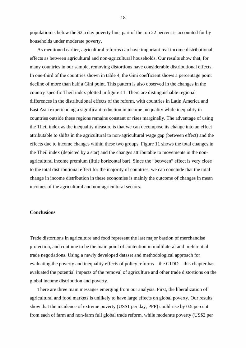
As mentioned earlier, agricultural reforms can have important real income distributional
effects as between agricultural and non-agricultural households. Our results show that, for
many countries in our sample, removing distortions have considerable distributional effects.
In one-third of the countries shown in table 4, the Gini coefficient shows a percentage point
decline of more than half a Gini point. This pattern is also observed in the changes in the
country-specific Theil index plotted in figure 11. There are distinguishable regional
differences in the distributional effects of the reform, with countries in Latin America and
East Asia experiencing a significant reduction in income inequality while inequality in
countries outside these regions remains constant or rises marginally. The advantage of using
the Theil index as the inequality measure is that we can decompose its change into an effect
attributable to shifts in the agricultural to non-agricultural wage gap (between effect) and the
effects due to income changes within these two groups. Figure 11 shows the total changes in
the Theil index (depicted by a star) and the changes attributable to movements in the non-
agricultural income premium (little horizontal bar). Since the “between” effect is very close
to the total distributional effect for the majority of countries, we can conclude that the total
change in income distribution in these economies is mainly the outcome of changes in mean
incomes of the agricultural and non-agricultural sectors.
Conclusions
Trade distortions in agriculture and food represent the last major bastion of merchandise
protection, and continue to be the main point of contention in multilateral and preferential
trade negotiations. Using a newly developed dataset and methodological approach for
evaluating the poverty and inequality effects of policy reforms—the GIDD—this chapter has
evaluated the potential impacts of the removal of agriculture and other trade distortions on the
global income distribution and poverty.
There are three main messages emerging from our analysis. First, the liberalization of
agricultural and food markets is unlikely to have large effects on global poverty. Our results
show that the incidence of extreme poverty (US$1 per day, PPP) could rise by 0.5 percent
from each of farm and non-farm full global trade reform, while moderate poverty (US$2 per

19
day, PPP) is likely to fall by 0.9 percent from agricultural reform alone. The second message
is that these small aggregate changes are produced by a combination of offsetting trends at
the regional and national levels. Farmers in Latin America—the region that accounts for less
than 5 percent of global poverty—experience significant income gains, while 15 million more
people in South Asia—where half of the world’s poor reside—would fall below the extreme
poverty line from freeing world agricultural markets and another 2.8 million if barriers to
non-farm goods trade also were to be removed. There are some countries or regions that
would experience considerable distributional changes following global trade reform.
Inequality is projected to fall in regions such as Latin America, which are characterized by
high initial inequality, and is projected to rise in South Asia which is characterized by low
initial inequality. As a result, the projected changes for developing countries as a group are
small overall.
There are several important caveats to our analysis. First, it should be emphasized that,
although poverty reduction is a most worthy goal, it should not be the only, or even the first,
metric with which to measure trade policy. Trade reform cannot be expected to benefit all
constituents, and can only do so only if accompanied by other complimentary domestic
policies. Second, our analysis is confined to examination of the effects of static efficiency
gains only, and does not consider the potential growth effects of trade liberalization.
Although our results show that the static gains from agricultural and other trade reform may
not contribute to a reduction in extreme poverty and may do little to combat moderate
poverty, they do not imply that this pattern of trade liberalization cannot be an effective tool
for poverty reduction. Finally, our micro-simulation model considers only changes in labor
income: while this is the most important income source for households at or near the poverty
line, accounting for changes in other factor returns may yield somewhat different inequality
results.
References
Anderson, K. (ed.) (2009), Distortions to Agricultural Incentives: A Global Perspective,
1955-2007, London: Palgrave Macmillan and Washington DC: World Bank.
Anderson, K. and W. Martin (2005), “Agricultural Trade Reform and the Doha Development
Agenda”, The World Economy 28(9): 1301–27.

20
Anderson K. and E. Valenzuela (2008),”Estimates of Global Distortions to Agricultural
Incentives, 1955 to 2007”, World Bank, Washington DC, October, accessible at
www.worldbank.org/agdistortions.
Anderson, K., E. Valenzuela and D. van der Mensbrugghe (2010), “Global Welfare and
Poverty Effects Using the Linkage Model”, Ch. 2 in this volume.
Bourguignon, F. and L. P. da Silva (eds.) (2003), The Impact of Economic Policies on
Poverty and Income Distribution: Evaluation Techniques and Tools, Washington DC:
World Bank and London: Oxford University Press.
Bussolo, M., R. De Hoyos and D. Medvedev (2008), “Economic Growth and Income
Distribution: Linking Macroeconomic Models with Household Survey Data at the
Global Level.” Paper presented at the 30th general conference of the International
Association for Research in Income and Wealth (IARIW), Portoroz, Slovenia, 24-30
August.
Bussolo, M., R. De Hoyos, D. Medvedev and D. van der Mensbrugghe (2007), “Global
Growth and Distribution: Are China and India Reshaping the World?” World Bank
Policy Research Working Paper 4392, Washington DC: World Bank.
Bussolo, M., J. Lay and D. van der Mensbrugghe (2005), “Structural Change and Poverty
Reduction in Brazil: The Impact of the Doha Round”, pp. 249-285 (Ch. 9) in T.W.
Hertel and L.A. Winters (eds.) Poverty and the WTO: Impacts of the Doha
Development Agenda, London: Palgrave Macmillan and Washington DC: World
Bank.
Chen, S. and M. Ravallion (2003), “Household Welfare Impacts of China’s Accession to the
World Trade Organization”, World Bank Economic Review 18(1): 29-57.
Chen, S. and M. Ravallion (2007), ‘Absolute Poverty Measurtes for the Developing World,
1981-2004’, Policy Research Working Paper 4211, World Bank, Washington DC,
April.
De Hoyos, R.E. (2007), “North-South Trade Agreements and Household Welfare: Mexico
under NAFTA”, mimeo, World Bank, Washington DC.
Ferreira, F.H.G. and P.G. Leite (2003), “Meeting the Millennium Development Goals in
Brazil: Can Microsimulations Help?” Economía 3(2): 235–79.

21
Ferreira, F.H.G. and P.G. Leite (2004), “Educational Expansion and Income Distribution: A
Microsimulation for Ceará,”, pp. 222-50 in A. Shorrocks and R. van der Hoeven
(eds.), Growth, Inequality and Poverty, London: Oxford University Press.
Krueger, A.O., M. Schiff and A. Valdés (1988), “Measuring the Impact of Sector-specific
and Economy-wide Policies on Agricultural Incentives in LDCs”, World Bank
Economic Review 2(3): 255-72.
McCulloch, N., L.A. Winters and X. Cirera (2001), Trade Liberalization and Poverty: A
Handbook, London: Centre for Economic Policy Research.
Nicita, A. (2004), “Who Benefited From Trade Liberalization in Mexico? Measuring the
Effects on Household Welfare”, Policy Research Working Paper 3265, World Bank,
Washington DC.
Ravallion, M. and S. Chen (2003), “Measuring Pro-poor Growth”, Economics Letters 78: 93-
99.
Rodrik D. (1998), “Why Is Trade Reform So Difficult in Africa?” Journal of African
Economies 7(1): 43-69.
Valenzuela, E. and K. Anderson (2008), ‘Alternative Agricultural Price Distortions for CGE
Analysis of Developing Countries, 2004 and 1980-84’, Research Memorandum No.
13, Center for Global Trade Analysis, Purdue University, West Lafayette IN
https://www.gtap.agecon.purdue.edu/resources/res_display.asp?RecordID=2925
van der Mensbrugghe, D. (2005), ‘LINKAGE Technical Reference Document: Version 6.0’,
Unpublished, World Bank, Washington DC, January, accessible at
www.worldbank.org/prospects/linkagemodel
van der Mensbrugghe, D., E. Valenzuela and K. Anderson (2010), ‘Border Price and Export
Demand Shocks for Developing Countries from Rest-of-World Trade Liberalization
Using the Linkage Model’, Appendix to this volume.
Winters, L.A. (2002), “Trade, Trade Policy and Poverty: What Are the Links?” The World
Economy 25(9): 1339-68.

22
Figure 1: Income distributions for agricultural and non-agricultural populations of the world, 2000
0
.1.2
.3.4
Den
sity
1 3 5 7 9Monthly household per capita income (1993 PPP, log)
Poverty Line
Global Income Distribution, 2000 Global Agricultural Population
Global Non-Agricultural Population
Source: Authors’ compilation using GIDD

23
Figure 2: Relationship between income levels and employment in agriculture, by country, 2000
(proportion of national workforce employed in agriculture)
0.2
.4.6
.8
0 500 1000 1500Monthly household per capita income (1993 PPP)
Area of symbol proportional to the country's population
China
India
Brazil EU US
Russia
Source: Authors’ compilation using GIDD

24
Figure 3: Share of population in agriculture and income share, by developing country, 2000
(percent)
0 10 20 30 40 50 60 70 80 90 100
BulgariaRussian Federation
JordanMexico
HungaryBelarusEstonia
EcuadorPoland
MauritaniaChile
Venezuela, RBBrazil
LithuaniaRomania
BeninPanamaSenegalUkraine
El SalvadorSouth Africa
ColombiaCosta Rica
JamaicaDominican Republic
GuineaMacedonia, FYR
MaliPeru
TajikistanBolivia
ParaguayTurkey
IndonesiaNicaraguaSri Lanka
AzerbaijanArmenia
HondurasKazakhstanUzbekistanGuatemalaPhilippines
MoroccoGeorgiaThailand
HaitiGhana
IndiaMoldovaPakistan
Cote d'IvoireNigeria
Gambia, TheAlbaniaGuyana
Kyrgyz RepublicYemen, Rep.
CameroonUganda
BangladeshVietnam
CambodiaMadagascar
KenyaEthiopia
TanzaniaNepal
Lao PDRBurkina Faso
Burundi
Agriculture incomes (% of total)
Agriculture population (% of total)
Source: Authors’ compilation using GIDD (showing only developing countries and transition economies).

25
Figure 4: Inequality variation in agricultural, nonagricultural and all households, by developing country, 2000
(Gini coefficient)
0.15
0.25
0.35
0.45
0.55
0.65
Den
mar
kFi
nlan
dSw
eden
Net
herla
nds
Kor
ea, R
ep.
Aus
tria
Luxe
mbo
urg
Ger
man
yA
lban
iaFr
ance
Tajik
ista
nSw
itzer
land
Can
ada
Aus
tralia EU
Spai
nG
reec
eIta
lyN
ew Z
eala
ndG
eorg
iaPo
rtuga
lG
hana
Isra
elN
iger
iaU
nite
d St
ates
Sing
apor
eC
hina
Hon
g K
ong,
…G
ambi
a, T
heEl
Sal
vado
rM
exic
oN
icar
agua
Col
ombi
aEc
uado
rB
oliv
iaB
razi
lG
uate
mal
aH
unga
ryU
krai
neC
zech
Rep
ublic
Slov
enia
Paki
stan
Bel
arus
Rus
sian
…R
oman
iaK
yrgy
z R
epub
licLi
thua
nia
Arm
enia
Kaz
akhs
tan
Ethi
opia
Bul
garia
Pola
ndM
ongo
liaB
angl
ades
hEs
toni
aIn
dia
Indo
nesi
aY
emen
, Rep
.Ir
elan
dU
zbek
ista
nM
oldo
vaTa
nzan
iaV
ietn
amLa
o PD
RN
epal
Ben
inA
zerb
aija
nTu
rkey
Mac
edon
ia, F
YR
Sri L
anka
Uni
ted
Kin
gdom
Mor
occo
Mal
iSe
nega
lG
uine
aTh
aila
ndM
aurit
ania
Jam
aica
Guy
ana
Cam
bodi
aJo
rdan
Bur
undi
Ven
ezue
la, R
BU
gand
aC
amer
oon
Ken
yaC
ote
d'Iv
oire
Cos
ta R
ica
Mad
agas
car
Phili
ppin
esB
urki
na F
aso
Dom
inic
an …
Peru
Chi
leH
ondu
ras
Pana
ma
Para
guay
Sout
h A
fric
aH
aiti
Gini in agriculture (-) Gini in non-agriculture (x)
Overall Gini (♦ )
Source: Authors’ compilation using GIDD.
26
Figure 5: GIDD methodological framework
Removal of Global Agricultural Distortions
CGE – LINKAGE
Growth Effects
Real Wages (by skill and sector)
Hypothetical Income Distribution
Food Prices
Source: Authors’ construction.

27
Figure 6: Effects on national real consumption of removal globally of agricultural and all merchandise trade distortions (percent)
Note: The black bars show the percent increase in consumption (at pre-reform prices) due to the removal of price and trade distortions in agriculture and food products (excluding beverages and tobacco). The grey bars show the additional gains in consumption due to the removal of all remaining barriers to merchandise trade. The combined length of the two bars shows the consumption gains from global trade reform of all merchandise.
-4.0 -2.0 0.0 2.0 4.0 6.0 8.0 10.0
EcuadorLithuania
New ZealandBulgaria
NigeriaRest of North Africa
ColombiaRest of Western Europe
ArgentinaMozambique
SlovakiaEstonia
Czech RepublicBrazil
MoroccoSlovenia
PolandRussia
Rest of East AsiaVietnam
NicaraguaHungaryMalaysiaThailand
ZimbabweLatvia
Rest of LACKorea
IndonesiaRest of ECAKazakhstanPhilippines
Middle EastEU 15
BangladeshRomania
TurkeyAustralia
JapanZambiaCanada
Rest of Sub-Saharan AfricaTanzania
TaiwanPakistan
IndiaHong Kong and Singapore
United StatesEgypt
South AfricaOther South Asia
Sri LankaMexico
ChinaRest of West & Central Africa
ChileMadagascar
UgandaSenegal
Kyrgystan
Percent change in real consumption
Global liberalization of trade in agriculture and food products
Global liberalization of all trade
Source: Authors’ compilation using Linkage model results similar to those in Anderson, Valenzuela and van der Mensbrugghe (2010) except with more-limited factor mobility.

28
Figure 7: Effects on national real factor rewards of removal globally of just agricultural price and trade policies (percent)
-4.0 -3.0 -2.0 -1.0 0.0 1.0 2.0 3.0 4.0 5.0
ArgentinaEcuador
MozambiqueNew Zealand
ColombiaBulgaria
PhilippinesVietnam
ZimbabweKazakhstanMiddle East
BrazilRest of LAC
ThailandChina
Rest of North AfricaRest of East Asia
AustraliaRest of ECA
Hong Kong and SingaporeCanada
IndonesiaChile
SenegalEgypt
United StatesMalaysia
MexicoEstonia
South AfricaPakistan
Other South AsiaKyrgystan
SloveniaNicaragua
TaiwanTanzania
West & Central AfricaJapan
Rest of Western EuropeRussiaLatvia
Sri LankaZambia
BangladeshRomania
EU 15Slovakia
Rest of Sub-Saharan AfricaKorea
TurkeyHungary
LithuaniaCzech Republic
IndiaUgandaPolandNigeria
MadagascarMorocco
Percent change in real value added
Unskilled Agri LaborUnskilled Non-agri LaborSkilled Agri LaborSkilled Non-Agri LaborCapitalLand
Note: Each bar shows a contribution of changes in value added of a specific factor to the total change in value added, deflated by the price of GDP at factor cost. Countries are sorted (in descending order) by the increase in payments to unskilled farm labor. Source: Authors’ compilation using Linkage model results similar to those in Anderson, Valenzuela and van der Mensbrugghe (2010) except with more-limited factor mobility.

29
Figure 8: National Growth Incidence Curves: effects on per capita household income distribution of a hypothetical 1 percent increase in agricultural versus nonagricultural incomes in developing countries
(percent change in income)
0.2
.4.6
.81
1% increase in nonagricultural incomes
1% increase in agricultural incomes
0 20 40 60 80 100Percentiles
Vertical line represents the extreme poverty line
Source: Authors’ compilation using GIDD (dataset for developing countries only).

30
Figure 9: Regional and National Growth Incidence Curves: effects on per capita household income distribution of full global agricultural policy reform
(percent change in income)
(a) Regional -2
02
46
810
12%
Cha
nge
in P
er-c
apita
Inco
me
0 20 40 60 80 100Percentiles
% of poor in Latin America
% of poor in South Asia
Latin America Other developing countries
South Asia
(b) National: Brazil and India
% of poor in India
% of poor in Brazil
India Brazil
Source: Authors’ compilation using GIDD (dataset for developing countries only).

31
Figure 10: Poverty changes as a share of the total change among the most losing/winning developing countries from full global agricultural policy reform
(percent)
Share of the global increase in poverty
India
Mexico
South Africa Kenya
Pakistan
Morocco
Bangladesh
Turkey
Sri Lanka
RoW
100806040200
1.0
0.2
0.3
0.5
0.7
0.7 0.7 1.8
2.2
92.0
Share of the global reduction in poverty
Philippines Brazil
Indonesia Nigeria
Thailand Peru
Vietnam
Yemen
Ecuador
RoW Colombia
403020100
10.1
1.6
1.9 2.1
2.1
5.5
6.1
8.3
11.5
12.1
38.6
Source: Authors’ compilation using GIDD (dataset for developing countries only).

32
Figure 11: Theil Indexa of overall and between-group income distributional changes from full global agricultural policy reform
-0.035
-0.025
-0.015
-0.005
0.005
Yem
en, R
epub
lic o
fH
aiti
Vie
tnam
Hon
dura
sG
uate
mal
aPe
ruPh
ilipp
ines
Para
guay
Thai
land
Ecua
dor
Jord
anC
ambo
dia
Bra
zil
Col
ombi
aB
oliv
iaG
uyan
aJa
mai
caD
omin
ican
Rep
ublic
El S
alva
dor
Cos
ta R
ica
Kaz
akhs
tan
Pana
ma
Aze
rbai
jan
Ven
ezue
la, R
ep. B
ol.
Chi
na,P
.R.:
Mai
nlan
dK
yrgy
z R
epub
licG
eorg
iaR
ussi
aM
oldo
vaU
krai
neA
lban
iaTa
jikis
tan
Bul
garia
Indo
nesi
aC
hile
Sene
gal
Tanz
ania
Uzb
ekis
tan
Mon
golia
Mau
ritan
iaC
ôte
d'Iv
oire
Ben
inG
uine
aPa
kist
anM
ali
Rom
ania
Gha
naN
icar
agua
Gam
bia,
The
Cam
eroo
nM
exic
oB
urki
na F
aso
Nep
alSr
i Lan
kaEs
toni
aA
rmen
iaN
iger
iaU
gand
aH
unga
ryTu
rkey
Bur
undi
Sout
h A
fric
aPo
land
Ban
glad
esh
Indi
aK
enya
Ethi
opia
Lith
uani
a
0.015
Change in the overall Theil index
Change in the between-group (agri / non-agri) component of the Theil index
a The Theil Index is an inequality measure of the family of general entropy which has the property of yielding perfectly additive inequality decompositions by population subgroups.
Source: Authors’ compilation using GIDD (dataset for developing countries only).

33
Table 1: Characteristics of the poor for agricultural and nonagricultural households of developing countries, 2000
Pop’n share (%)
Primary school completed by
household head (%)
Age of household
head (years)
Number of people in household
Share of households with female
head (%) Agricultural 44.8 32.3 44.8 7.11 8.7
Non-Agricultural 55.2 46.0 44.4 7.06 14.0
Source: Authors’ compilation using GIDD.

34
Table 2: Effects of removing agricultural and all merchandise trade distortions on global poverty and inequality
(percentage point change)
Initial levels:
Gini coefficient
(%)
Real average monthly income (2000, US$ PPP)
$1 a day poverty
incidence (%)
$1 a day poverty share (%)
$2 a day poverty
incidence (%)
$2 a day poverty share (%)
Agricultural 0.45 65 31.5 76 73.8 70 Nonagricultural 0.63 320 8.3 24 26.7 30 All households 0.67 204 18.9 100 48.2 100 Agricultural liberalization, difference from baseline (percentage points): Agricultural 0.7 1.1a 0.86 1.13 -0.86 0.47 Nonagricultural -0.1 0.2a -0.29 -1.13 -0.90 -0.47 All households -0.1 0.3a 0.23 0.00 -0.88 0.00 All merchandise trade liberalization, difference from baseline (percentage points): Agricultural 0.8 0.8a 1.09 1.02 -0.66 0.57 Nonagricultural -0.2 0.4a -0.19 -1.02 -0.95 -0.57 All households -0.0 0.4a 0.39 0.00 -0.82 0.00
a Changes in average income are expressed in percentages. Source: Authors’ compilation using Linkage model results similar to those in Anderson, Valenzuela and van der Mensbrugghe (2010)except with more-limited factor mobility, and GIDD data.

35
Table 3: Effects of removing agricultural and all merchandise trade distortions on the incidence of poverty using the GIDD model, by region
Share of
global Change in no. of poor from global trade reform of: (a)extremely poor poverty Agriculture only All merchandise (<$1 a day) (%) (million) (%) (million) (%)East Asia 24 -6.4 -2.8 -6.3 -2.8South Asia 50 15.4 3.3 18.2 3.9Sub-Saharan Africa 21 -1.0 -0.5 0.5 0.3Latin America 4 -2.8 -6.9 -3.5 -8.7Globala 100 5.0 0.5 8.9 1.0 (b)moderately and extremely poor (<$2 a day) (%) (million) (%) (million) (%)East Asia 33 -12.8 -1.6 -13.2 -1.7South Asia 46 -3.6 -0.3 -2.0 -0.2Sub-Saharan Africa 14 0.1 0.0 1.1 0.3Latin America 4 -4.8 -4.6 -5.7 -5.4Globala 100 -22.1 -0.9 -19.8 -0.8
. a Includes Middle East & North Africa, Eastern Europe & Central Asia, and high-income countries, which together account for no more than 2 percent of the world’s poor.
Source: Authors’ compilation using Linkage model results similar to those in Anderson, Valenzuela and van der Mensbrugghe (2010) except with more-limited factor mobility, and GIDD data.

36
Table 4: Effects of full global liberalization of agricultural and all merchandise trade on the incidence of inequality and poverty, by developing country
(percentage point change)
Agriculture-only reform All merchandise trade reform Gini
coefficient <$1 a day headcount
<$2 a day headcount
Gini coefficient
<$1 a day headcount
<$2 a day headcount
East Asia
-0.72 -0.38 -0.76 -0.62 -0.37 -0.78
Cambodia -0.75 -0.40 0.17 -0.69 -0.90 -0.05China -0.37 0.00 0.00 -0.35 0.00 0.00Indonesia 0.05 -0.49 -0.83 0.04 -0.57 -1.26Philippines -6.88 -6.31 -9.91 -6.65 -6.15 -9.80Thailand -1.25 -0.40 -2.29 -1.10 -0.38 -2.29Vietnam -1.85 -0.89 -3.57 0.08 -0.66 -2.97
South Asia 0.82 1.16 -0.27 0.81 1.37 -0.15Bangladesh 0.46 0.06 -0.19 -0.09 0.07 0.05India 1.01 1.49 -0.33 1.04 1.71 -0.26Nepal 0.05 -0.12 0.04 0.05 0.11 0.18Pakistan 0.04 0.09 0.03 0.10 0.49 0.44Sri Lanka 0.03 0.14 -0.01 0.17 -0.20 -0.69
Sub-Saharan Africa -0.04 -0.23 0.02 0.06 0.11 0.25
Burundi 0.27 -0.35 0.17 0.26 0.12 0.37Benin 0.00 -0.05 0.09 0.02 0.79 0.74Burkina Faso -0.02 0.00 0.05 0.02 0.78 0.43Cote d'Ivoire 0.02 0.14 0.61 0.06 0.43 0.89Cameroon -0.01 0.24 0.06 0.05 0.72 0.70Ethiopia -0.13 -0.27 -0.20 -0.07 0.24 0.22Ghana 0.08 0.10 0.09 0.08 0.62 0.62Guinea -0.04 -0.10 0.04 0.03 0.62 0.42Gambia, The -0.12 0.05 0.00 -0.11 0.61 0.40Kenya 0.30 0.41 0.54 0.38 0.52 0.94Madagascar 0.95 0.24 0.06 0.98 0.56 0.36Mali 0.01 -0.01 -0.03 0.03 0.93 0.45Mauritania 0.03 0.09 0.18 0.07 0.60 0.60Nigeria 0.10 -1.04 -0.30 0.27 -0.75 -0.21Senegal -0.28 -0.12 -0.24 0.01 0.75 0.31Tanzania -0.03 0.01 0.03 0.02 0.54 0.26Uganda 0.30 -0.05 0.01 0.45 0.12 -0.03South Africa 0.32 0.68 0.68 0.21 0.39 0.50

37
Table 3.4 (continued): Effects of full global liberalization of agricultural and all merchandise trade on the incidence of inequality and poverty, by developing/transition economy
(percentage point change)
Agriculture-only reform All merchandise trade reform Gini
coefficient <$1 a day headcount
<$2 a day headcount
Gini coefficient
<$1 a day headcount
<$2 a day headcount
Latin America -0.51 -0.61 -1.06 -0.65 -0.77 -1.26Bolivia -0.55 -0.64 -0.65 -0.71 -0.74 -0.61Brazil -0.58 -0.82 -1.16 -0.70 -0.92 -1.31Chile 0.03 0.02 0.02 0.09 -0.02 -0.10Colombia -0.71 -0.45 -1.30 -0.85 -0.49 -1.40Costa Rica -0.56 -0.13 -0.50 -0.72 -0.22 -0.62Dominican Rep. -0.76 -0.24 -0.75 -0.95 -0.24 -0.89Ecuador -0.90 -1.75 -2.78 -1.29 -1.98 -3.09El Salvador -1.09 -1.25 -0.79 -1.29 -1.34 -0.88Guatemala -0.87 -1.26 -1.54 -1.11 -1.59 -1.44Guyana -1.49 -0.27 -0.39 -1.66 -0.46 -0.54Honduras -1.06 -0.57 -1.58 -1.30 -0.72 -1.63Haiti -0.80 -0.61 -0.55 -1.04 -0.65 -0.53Jamaica -0.75 -0.10 -1.44 -0.91 -0.05 -1.49Mexico 0.20 0.36 0.35 -0.05 0.01 -0.07Nicaragua -2.42 -3.03 -1.42 -2.38 -3.07 -1.42Panama -0.40 -0.44 -0.74 -0.53 -0.51 -0.85Peru -1.21 -2.92 -6.41 -1.51 -3.10 -6.77Paraguay -0.77 -1.30 -1.41 -0.99 -1.38 -1.92Venezuela -0.29 -0.44 -0.71 -0.42 -0.55 -0.82Europe’s transition econs. 0.07 -0.02 -0.26 0.22 0.00 -0.12
Armenia 0.42 0.34 0.14 0.45 0.23 0.13Azerbaijan -0.23 0.10 -1.36 -0.12 0.14 -1.21Georgia -0.48 -0.49 -0.57 -0.37 -0.45 -0.61Kazakhstan -0.97 -0.39 -2.07 -1.00 -0.43 -2.22Kyrgyz Republic -0.50 0.08 0.57 -0.27 0.19 1.09Moldova -0.20 -0.22 -0.75 -0.06 -0.09 -0.24Russian Fed. -0.16 0.00 -0.32 -0.06 0.00 -0.31Tajikistan -0.12 -0.77 -0.75 -0.32 -0.67 -0.74Ukraine -0.11 -0.03 -0.33 -0.02 0.00 -0.04Uzbekistan -0.07 0.00 -0.06 0.29 0.00 0.03
World -0.1 0.23 -0.88 -0.0 0.39 -0.82Source: Authors’ compilation using Linkage model results similar to those in Anderson, Valenzuela and van der Mensbrugghe (2010) except with more-limited factor mobility, and GIDD data.