distributional impacts of the self-sufficiency project · distributional impacts of the...

Journal of Public Economics 92 (2008) 748–765www.elsevier.com/locate/econbase

Distributional impacts of the Self-Sufficiency Project☆

Marianne P. Bitler a,d, Jonah B. Gelbach b, Hilary W. Hoynes c,d,⁎

a University of California—Irvine, United Statesb University of Arizona, United States

c University of California, Davis, United Statesd NBER, United States

Received 4 January 2006; received in revised form 8 January 2007; accepted 19 July 2007Available online 27 July 2007

Abstract

A large literature has been concerned with the impacts of recent welfare reforms on income, earnings, transfers, and labor-forceattachment. While one strand of this literature relies on observational studies conducted with large survey-sample data sets, asecond makes use of data generated by experimental evaluations of changes to means-tested programs. Much of the overallliterature has focused on mean impacts. In this paper, we use random-assignment experimental data from Canada's Self-SufficiencyProject (SSP) to look at impacts of this unique reform on the distributions of income, earnings, and transfers. SSP offered membersof the treatment group a generous subsidy for working full time. Quantile treatment effect (QTE) estimates show there wasconsiderable heterogeneity in the impacts of SSP on the distributions of earnings, transfers, and total income; this heterogeneitywould be missed by looking only at average treatment effects. Moreover, these heterogeneous impacts are consistent with thepredictions of labor supply theory. During the period when the subsidy is available, the SSP impact on the earnings distribution iszero for the bottom half of the distribution. The quantiles of the SSP earnings distribution are higher for much of the upper third ofthe distribution except at the very top, where the quantiles of the earnings distribution are the same under either program orpossibly lower under SSP. Further, during the period when SSP receipt was possible, the impacts on the quantiles of thedistributions of transfer payments (Income Assistance plus the subsidy) and total income (earnings plus transfers) are also differentat different points of the distribution. In particular, positive impacts on the quantiles of the transfer distribution are concentrated atthe lower end of the transfer distribution, while positive impacts on the quantiles of the income distribution are concentrated in theupper end of the income distribution. Impacts of SSP on these distributions were essentially zero after the subsidy was no longeravailable.© 2007 Elsevier B.V. All rights reserved.

Keywords: Welfare programs; Labor supply; Policy evaluation; Heterogenous treatment effects

☆ We are grateful to Human Resources Development Canada for funding this experiment and to SRDC for research support and for making the SSPdata available. We thank Joshua Angrist, David Brownstone, David Green, Jeff Smith, Douglas Tattrie, and Kevin Milligan for helpful conversations,participants at Berkeley, Koc University, EALE, Irvine, PPIC, San Diego, SOLE, and the IZA/IFAU Conference on Program Evaluation for helpfulcomments, and Peter Huckfeldt for research assistance. All conclusions in this paper are solely the responsibility of the authors, and do not representthe opinions or conclusions of HDRC, SRDC, the Canadian government, the sponsors of the Self-Sufficiency Project, or any other institution.⁎ Corresponding author. UC Davis, Department of Economics, 1152 Social Sciences and Humanities Building, One Shields Avenue, Davis, CA

95616-8578, United States. Tel.: +1 530 752 3226; fax: +1 530 752 9382.E-mail addresses: [email protected] (M.P. Bitler), [email protected] (J.B. Gelbach), [email protected] (H.W. Hoynes).

0047-2727/$ - see front matter © 2007 Elsevier B.V. All rights reserved.doi:10.1016/j.jpubeco.2007.07.001

mailto:mbitler@uci.�edu

mailto:[email protected]

mailto:[email protected]

http://dx.doi.org/10.1016/j.jpubeco.2007.07.001

749M.P. Bitler et al. / Journal of Public Economics 92 (2008) 748–765

1. Introduction

As we move into the 21st century, government assistance for poor families has undergone major reform acrossEurope, Canada and the United States. In some cases, changes have taken place within traditional government welfareprograms (e.g., the SSP demonstration in Canada and welfare reform in the United States) to reduce the negative workincentives embodied in programs that tax away welfare benefits at a high rate with each extra dollar in earnings. Inother cases, new programs have been added or expanded, providing in-work subsidies for low income workers andfamilies. Prominent examples of these policies are the United States' Earned Income Tax Credit and the UnitedKingdom's Working Family Tax Credit. Further, a recent report identifies nine OECD countries (including the UnitedStates and United Kingdom) that offer in-work subsidies (Owens, 2005). A common feature of these program changesis expanding the financial gains to working. In so doing, the goal of the policy changes is to ‘make work pay’ andincrease self sufficiency.

In this dynamic policy environment, a large literature has developed.1 A common feature of this literature is thefocus on the mean impacts of the policy of interest. In this paper, we make an important contribution to the literature byusing a simple nonparametric estimator – quantile treatment effects, or QTEs – to estimate the impact of the SSPprogram on the distribution of earnings, hours worked, wages, transfers, and income.

In this paper, we contribute to the literature on the impacts of financial incentives on labor supply and to our ownearlier work on estimating distributional impacts (Bitler et al., 2006) in two ways. First, SSP is an important policy thathas received a great deal of attention in the international policy arena, influencing adoption of new policies andexperiments in Europe. The minimum work requirement and relatively generous benefits in SSP make the policyunique and have important implications for the impacts of the policy. For example, SSP moved long term recipientsinto the labor force while nearly paying for itself, costing a scant $4000 more per recipient over a 5-year period than thepreexisting welfare program (Michalopoulos et al., 2002). Our distributional analysis adds to our understanding of SSPin a fundamental way and provides a powerful test of the (expected) heterogeneity in labor supply effects.2 Second, theSSP experiment is unusual in that it provides data on wages and hours (other experiments tend to provide data only onearnings) thereby allowing for a much richer analysis of the labor supply implications relative to our earlier work(Bitler et al., 2006).

SSP was designed to test the impact of a generous earnings subsidy for full-time work on long-term welfareparticipants. The subsidy was evaluated through a randomized experiment which was sponsored by Human ResourcesDevelopment Canada and conducted by the Social Research Demonstration Corporation. Between 1992 and 1995, SSPrandomly assigned a group of single-parent recipients and applicants for welfare benefits (called Income Assistance orIA) in two provinces, New Brunswick and British Columbia, to treatment and control groups. Control group membersfaced the rules of IA in their home province. Treatment group members who had been on IA for 12 of the previous13 months were eligible for a generous earnings supplement if within a year they could find full time work (at least30 hours a week) at or above the minimum wage. The earnings supplement was one-half the difference between theirearnings and a benchmark earnings level ($30,000 in New Brunswick and $37,000 in British Columbia) and wasavailable for 36 months. Persons receiving the supplement had to forego their IA payments, although if they gave upthe supplement, they could receive IA if they were otherwise eligible.

Several final reports (Michalopoulos et al., 2002; Ford et al., 2003), and a large number of research papers (e.g.,Blank et al., 2000; Card and Hyslop, 2005; Card et al., 2001; Connolly and Gottschalk, 2004; Foley, 2004; Foley andSchwartz, 2003; Harknett and Gennetian, 2003; Kamionka and Lacroix, 2005; Lise et al., 2005; Michalopoulos et al.,

1 For example, in the United States, Grogger and Karoly (2005) provide a summary of welfare reform and Hotz and Scholz (2003) and Eissa andHoynes (2006) provide reviews of the Earned Income Tax Credit. Blundell and Hoynes (2004) compare the United States' and United Kingdom'sin-work policies, and evaluations of the Working Family Tax Credit appear in Blundell et al. (2000, 2006), Brewer et al. (2005), Francesconi andvan der Klaauw (2007), Gregg and Harkness (2003), and Leigh (2007). Bargain and Orsini (2006) and Smith et al. (2003) use cross-country data toevaluate European reforms.2 Michalopoulos et al. (2002, 2005) examine the impact of SSP on poverty rates and on ranges of hours worked and hourly wage rates. While this

provides some insight into the distributional analysis, our analysis is more comprehensive in that it also analyzes impacts on earnings, income, andtransfers. We also examine the full 54 month follow-up period rather than analyzing data from a few months, making our results more representativeof the longer run impacts of SSP. Finally, their analyses focus mostly on wages among the employed. By contrast, we consider the distribution ofwages for everyone, which takes account of the changes in employment rates and allows for more clean interpretation of the results. Employment isaffected by the supplement, and without strong assumptions, the distribution among the employed is a mixture of effects along the extensive andintensive margins.

750 M.P. Bitler et al. / Journal of Public Economics 92 (2008) 748–765

2005; Zabel et al., 2006) have looked at the overall impacts of the SSP experiment on income, earnings, labor forceattachment, unemployment durations, wages, wage growth, job choice, and marriage. These papers find that theprogram increased employment, earnings, and income considerably during the years when the supplement wasavailable, while having little or no impacts after the supplement was no longer available.

The existing literature focuses on SSP's mean impacts, in the full sample and in demographic subgroups. Meanimpacts, however, may conceal heterogeneous impacts across the distribution of earnings and income. For example,SSP generates an increase in total income and net wages at 30 hours of work and above. The income gains aresubstantial — most families had after-tax annual incomes $3000–$7000 higher with SSP than they would have had ifthey had worked the same number of hours under IA (Michalopoulos et al., 2002). Static labor supply theory predictsthat this increase in nonlabor income would lead some recipients to increase work and leave IA, thereby increasingearnings and income. On the other hand, workers who would work full-time under IA-only assignment receive awindfall payment under SSP, which could lead to much smaller (and possibly negative) earnings effects based onstandard labor supply analysis.

In this paper, we move beyond mean impacts and examine the impacts of SSP on the distribution of earnings, hours,wages, transfers, and income using QTE estimation.3 We estimate the QTEs very simply as the difference in outcomesat various quantiles of the treatment (SSP) and control (IA-only) group distributions. Thus, QTEs tell us how theearnings distribution changes when we assign SSP treatment randomly. The QTE is a simple nonparametric estimatorthat requires only that the treatment is randomly assigned. As we discuss in more detail below, QTEs identify only theimpact of treatment on the distribution; this impact is distinct from, and in general not equal to, the distribution oftreatment effects (as well as other interesting estimates, such as the treatment effect on people whose control-groupoutcome would have been the median).

Our results show that the SSP program indeed had heterogeneous impacts across the earnings, hours, wages,transfer, and income distributions. During the period when the subsidy is available, the impact of SSP on the earningsdistribution is zero for the bottom half of the distribution. The SSP earnings distribution is higher for much of the upperthird of the distribution except at the very top, where the earnings distribution is the same under either program orpossibly lower under SSP. Importantly, the changes in the earnings distribution reflect changes in the hours and wagedistributions, suggesting changes in reservation wages and desired labor supply. Further, during the SSP receipt period,the impacts on the distributions of transfer payments (IA plus the subsidy) and total income (earnings plus transfers) arealso different at different points of these distributions. Positive impacts on the transfer distribution are concentrated atthe lower end of the transfer distribution. By contrast, positive impacts on the income distribution are concentrated atthe upper end of the income distribution, suggesting that within this group of long term welfare recipients, the programbenefited the top of the distribution more than the bottom.4 Impacts of SSP on these distributions were essentially zeroor negative after the subsidy was no longer available.5

We argue that these findings are consistent with labor supply theory — workers respond to the financial incentivesby changing their hours worked and, in some cases, reducing the reservation wages at which they will just be willing totake a job. We can explore these pathways more completely in this setting than in others because we have data on wagesand hours.

The remainder of this paper is organized as follows. In Section 2, we discuss the SSP experiment and the financialincentives in IA and SSP. In Section 3, we use theoretical predictions about labor supply to discuss the expected effectsof SSP on labor supply, welfare receipt, and income. Section 4 discusses the empirical methods and Section 5 describesour data and presents descriptive statistics and reviews the mean treatment effects. Our main QTE results are presentedin Section 6 and we conclude in Section 7.

3 A host of authors have used QTEs (e.g., Heckman et al., 1997; Firpo, 2007). Closest to our work is Friedlander and Robins (1997), Koenker andBilias (2001), and Bitler et al. (2006) who each use experimental data and estimate QTEs to evaluate government transfer programs. Friedlander andRobins evaluate the impact of employment training programs in early welfare-reform experiments on earnings and Koenker and Bilias evaluate theimpact of a reemployment bonus on unemployment durations. Bitler et al. (2006) examine the impact of a welfare-reform experiment in Connecticutin the mid-1990s on earnings, transfers, and total income.4 As we discuss below, a person whose transfer payments are at the bottom of the transfers distribution will not necessarily have income at the

bottom of the income distribution (in fact, we would typically expect the opposite to be true, and generally that is what we empirically find).5 Note that persons assigned to the supplement group could always obtain Income Assistance (indefinitely) if they were income eligible and not

receiving the supplement. This suggests that we might not see large “losers” in the supplement group as IA provided a safety net. This is in contrastto the findings for welfare recipients facing time limits in the post-TANF policy setting in the U.S. (Bitler et al., 2006).


2. SSP, income assistance, and the SSP experiment

The SSP experiment randomly assigned welfare recipients to a treatment group – who could obtain SSP – or acontrol group – who had access only to the existing Income Assistance (IA) program. We use data from the SSPRecipient sample which consists of about 6000 single parents aged 19 or older in British Columbia and NewBrunswick who had been on IA for at least 12 month of the last 13 months.6 Random assignment began in November1992 and ended in March 1995.

Income assistance was (at the time of the SSP experiment) Canada's universal cash safety net program available toall demographic groups.7 Benefits are means tested using income and asset tests, and eligibility thresholds and benefitlevels vary by province and family size. The IA benefit structure is typical of means-tested transfer programs and ischaracterized by a guaranteed income (the benefit received if the family has no other income) and a benefit reductionrate or phase-out rate leading to high work disincentives. The IA program is quite generous — in 1992 the annualguarantee for a single-parent family with one child was $11,352 in British Columbia and $8448 in New Brunswick. Forcomparison, at 1992 exchange rates, the New Brunswick benefit level for a family of two is higher than thecorresponding 1994 U.S. AFDC benefit level for every state but Alaska, Hawaii, and New York's Suffolk county andthe British Columbia one higher than for any state but Alaska. As is common with welfare programs, the long-runbenefit reduction rate was very high, leading to large work disincentives. Specifically, in 1992, IA recipients in NewBrunswick faced a 100% benefit reduction rate for every dollar earned over $200 per month. In British Columbia, thedisregard was also $200 a month while the benefit reduction rate was 75% for 12 out of each 36 months and 100% forthe other 24 months out of 36.

The SSP earnings supplement is a negative-income-tax style transfer payment with a minimum hours of workrestriction. The supplement is equal to one-half the difference between recipient earnings and a benchmark earningsamount. The annual benchmark was quite high-$37,000 in British Columbia and $30,000 in New Brunswick.Eligibility requires maintaining full-time work (an average of at least 30 hours a week over a four-week period) at oneor more jobs paying at least the minimum wage. Further, there was a limited time period to establish eligibility for thesupplement—to be eligible to receive SSP, recipients had to establish full-time work within 12 months after randomassignment. The experimental group had access to the supplement over the next 3 years. Supplement recipients couldnot receive IA at the same time as they received the supplement, but supplement recipients could return to IA at anytime (including at the end of the SSP period). Lastly, to target the program to long-term welfare recipients, eligibility forthe supplement required having been on IA for 12 of the past 13 months.

The SSP benefit was very generous, leading to large increases in the returns to work. For example, a single motherwith one child in British Columbia working 30 hours a week at the minimum wage ($5.50 an hour at the start of theexperimental period) would have monthly income of $1899 under SSP, compared to $946 if she did not work and amaximum of $1146 if she combined work with IA receipt. In New Brunswick, an SSP recipient working at theminimum wage (which increased to $5.50 in 1996 from $5.00) would experience similar increases in income comparedto combining work and IA.

3. Expected impacts of the SSP supplement

We examine potentially heterogeneous impacts of SSP on earnings, transfers, and income through the lens of twomodels. We begin with a static labor supply model where women can freely choose hours of work at the given offeredwage and offered wages are constant. (Note that we use women to refer to persons in the experiment for expediency:96% of those in our final sample were females.) We then discuss the expected impacts on wages using the dynamicsearch model in Card and Hyslop (2005). We should note that this section describes incentives for individuals and doesnot necessarily map directly into our QTE measures of impacts of SSP on the distributions.

6 We exclude the SSP Plus sample (293 observations) from our analysis because we wish to focus on the impact of the financial incentives in SSPalone, which may be confounded with the effects of the employment services also offered in SSP Plus (e.g., Michalopoulos et al., 2002). We alsoignore the SSPApplicant sample, made up of new applicants at the time of random assignment, who had to stay on welfare for 12 months to becomeeligible for the supplement.7 Information about IA is drawn from Barrett et al. (1996), Michalopoulos et al. (2002), and Ford et al. (2003). Between 1995 and 1996, recipients

in both provinces experienced changes in IA and other transfer programs. While the changes alter the magnitude of any expected effects, thechanges do not substantively impact any theoretical predictions about the effects of the supplement.

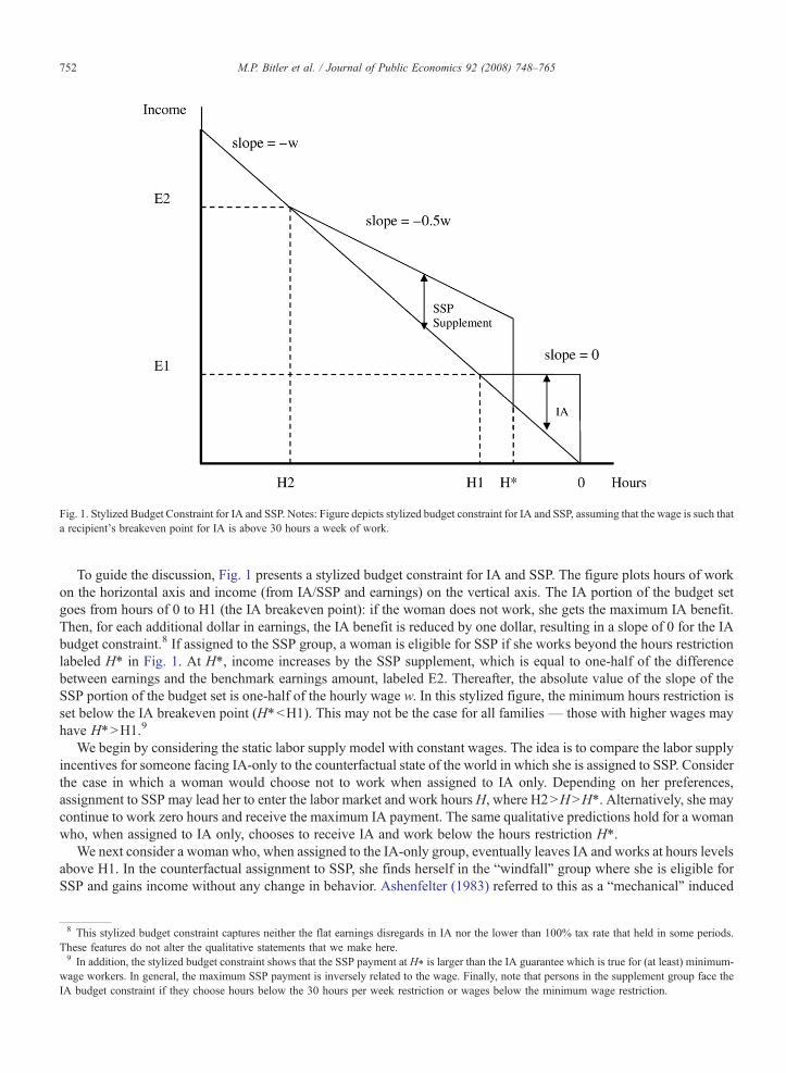
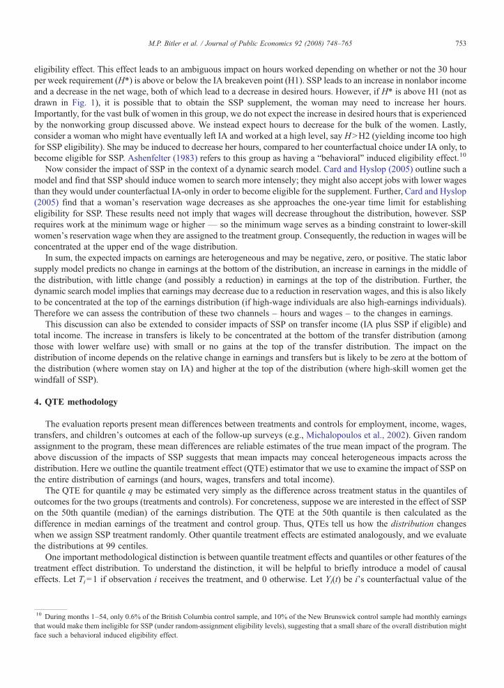
Fig. 1. Stylized Budget Constraint for IA and SSP. Notes: Figure depicts stylized budget constraint for IA and SSP, assuming that the wage is such thata recipient's breakeven point for IA is above 30 hours a week of work.


To guide the discussion, Fig. 1 presents a stylized budget constraint for IA and SSP. The figure plots hours of workon the horizontal axis and income (from IA/SSP and earnings) on the vertical axis. The IA portion of the budget setgoes from hours of 0 to H1 (the IA breakeven point): if the woman does not work, she gets the maximum IA benefit.Then, for each additional dollar in earnings, the IA benefit is reduced by one dollar, resulting in a slope of 0 for the IAbudget constraint.8 If assigned to the SSP group, a woman is eligible for SSP if she works beyond the hours restrictionlabeled H⁎ in Fig. 1. At H⁎, income increases by the SSP supplement, which is equal to one-half of the differencebetween earnings and the benchmark earnings amount, labeled E2. Thereafter, the absolute value of the slope of theSSP portion of the budget set is one-half of the hourly wage w. In this stylized figure, the minimum hours restriction isset below the IA breakeven point (H⁎bH1). This may not be the case for all families — those with higher wages mayhave H⁎NH1.9

We begin by considering the static labor supply model with constant wages. The idea is to compare the labor supplyincentives for someone facing IA-only to the counterfactual state of the world in which she is assigned to SSP. Considerthe case in which a woman would choose not to work when assigned to IA only. Depending on her preferences,assignment to SSP may lead her to enter the labor market and work hours H, where H2NHNH⁎. Alternatively, she maycontinue to work zero hours and receive the maximum IA payment. The same qualitative predictions hold for a womanwho, when assigned to IA only, chooses to receive IA and work below the hours restriction H⁎.

We next consider a woman who, when assigned to the IA-only group, eventually leaves IA and works at hours levelsabove H1. In the counterfactual assignment to SSP, she finds herself in the “windfall” group where she is eligible forSSP and gains income without any change in behavior. Ashenfelter (1983) referred to this as a “mechanical” induced

8 This stylized budget constraint captures neither the flat earnings disregards in IA nor the lower than 100% tax rate that held in some periods.These features do not alter the qualitative statements that we make here.9 In addition, the stylized budget constraint shows that the SSP payment at H⁎ is larger than the IA guarantee which is true for (at least) minimum-

wage workers. In general, the maximum SSP payment is inversely related to the wage. Finally, note that persons in the supplement group face theIA budget constraint if they choose hours below the 30 hours per week restriction or wages below the minimum wage restriction.


eligibility effect. This effect leads to an ambiguous impact on hours worked depending on whether or not the 30 hourper week requirement (H⁎) is above or below the IA breakeven point (H1). SSP leads to an increase in nonlabor incomeand a decrease in the net wage, both of which lead to a decrease in desired hours. However, if H⁎ is above H1 (not asdrawn in Fig. 1), it is possible that to obtain the SSP supplement, the woman may need to increase her hours.Importantly, for the vast bulk of women in this group, we do not expect the increase in desired hours that is experiencedby the nonworking group discussed above. We instead expect hours to decrease for the bulk of the women. Lastly,consider a woman who might have eventually left IA and worked at a high level, say HNH2 (yielding income too highfor SSP eligibility). She may be induced to decrease her hours, compared to her counterfactual choice under IA only, tobecome eligible for SSP. Ashenfelter (1983) refers to this group as having a “behavioral” induced eligibility effect.10

Now consider the impact of SSP in the context of a dynamic search model. Card and Hyslop (2005) outline such amodel and find that SSP should induce women to search more intensely; they might also accept jobs with lower wagesthan they would under counterfactual IA-only in order to become eligible for the supplement. Further, Card and Hyslop(2005) find that a woman's reservation wage decreases as she approaches the one-year time limit for establishingeligibility for SSP. These results need not imply that wages will decrease throughout the distribution, however. SSPrequires work at the minimum wage or higher — so the minimum wage serves as a binding constraint to lower-skillwomen's reservation wage when they are assigned to the treatment group. Consequently, the reduction in wages will beconcentrated at the upper end of the wage distribution.

In sum, the expected impacts on earnings are heterogeneous and may be negative, zero, or positive. The static laborsupply model predicts no change in earnings at the bottom of the distribution, an increase in earnings in the middle ofthe distribution, with little change (and possibly a reduction) in earnings at the top of the distribution. Further, thedynamic search model implies that earnings may decrease due to a reduction in reservation wages, and this is also likelyto be concentrated at the top of the earnings distribution (if high-wage individuals are also high-earnings individuals).Therefore we can assess the contribution of these two channels – hours and wages – to the changes in earnings.

This discussion can also be extended to consider impacts of SSP on transfer income (IA plus SSP if eligible) andtotal income. The increase in transfers is likely to be concentrated at the bottom of the transfer distribution (amongthose with lower welfare use) with small or no gains at the top of the transfer distribution. The impact on thedistribution of income depends on the relative change in earnings and transfers but is likely to be zero at the bottom ofthe distribution (where women stay on IA) and higher at the top of the distribution (where high-skill women get thewindfall of SSP).

4. QTE methodology

The evaluation reports present mean differences between treatments and controls for employment, income, wages,transfers, and children's outcomes at each of the follow-up surveys (e.g., Michalopoulos et al., 2002). Given randomassignment to the program, these mean differences are reliable estimates of the true mean impact of the program. Theabove discussion of the impacts of SSP suggests that mean impacts may conceal heterogeneous impacts across thedistribution. Here we outline the quantile treatment effect (QTE) estimator that we use to examine the impact of SSP onthe entire distribution of earnings (and hours, wages, transfers and total income).

The QTE for quantile q may be estimated very simply as the difference across treatment status in the quantiles ofoutcomes for the two groups (treatments and controls). For concreteness, suppose we are interested in the effect of SSPon the 50th quantile (median) of the earnings distribution. The QTE at the 50th quantile is then calculated as thedifference in median earnings of the treatment and control group. Thus, QTEs tell us how the distribution changeswhen we assign SSP treatment randomly. Other quantile treatment effects are estimated analogously, and we evaluatethe distributions at 99 centiles.

One important methodological distinction is between quantile treatment effects and quantiles or other features of thetreatment effect distribution. To understand the distinction, it will be helpful to briefly introduce a model of causaleffects. Let Ti=1 if observation i receives the treatment, and 0 otherwise. Let Yi(t) be i's counterfactual value of the

10 During months 1–54, only 0.6% of the British Columbia control sample, and 10% of the New Brunswick control sample had monthly earningsthat would make them ineligible for SSP (under random-assignment eligibility levels), suggesting that a small share of the overall distribution mightface such a behavioral induced eligibility effect.

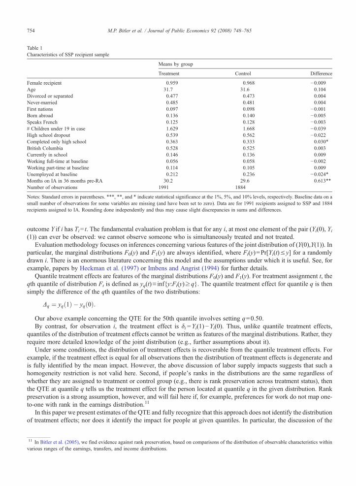
Table 1Characteristics of SSP recipient sample

Means by group

Treatment Control Difference

Female recipient 0.959 0.968 −0.009Age 31.7 31.6 0.104Divorced or separated 0.477 0.473 0.004Never-married 0.485 0.481 0.004First nations 0.097 0.098 −0.001Born abroad 0.136 0.140 −0.005Speaks French 0.125 0.128 −0.003# Children under 19 in case 1.629 1.668 −0.039High school dropout 0.539 0.562 −0.022Completed only high school 0.363 0.333 0.030⁎

British Columbia 0.528 0.525 0.003Currently in school 0.146 0.136 0.009Working full-time at baseline 0.056 0.058 −0.002Working part-time at baseline 0.114 0.105 0.009Unemployed at baseline 0.212 0.236 −0.024⁎Months on IA in 36 months pre-RA 30.2 29.6 0.613⁎⁎

Number of observations 1991 1884

Notes: Standard errors in parentheses. ⁎⁎⁎, ⁎⁎, and ⁎ indicate statistical significance at the 1%, 5%, and 10% levels, respectively. Baseline data on asmall number of observations for some variables are missing (and have been set to zero). Data are for 1991 recipients assigned to SSP and 1884recipients assigned to IA. Rounding done independently and thus may cause slight discrepancies in sums and differences.


outcome Y if i has Ti= t. The fundamental evaluation problem is that for any i, at most one element of the pair (Yi(0), Yi(1)) can ever be observed: we cannot observe someone who is simultaneously treated and not treated.

Evaluation methodology focuses on inferences concerning various features of the joint distribution of (Y(0),Y(1)). Inparticular, the marginal distributions F0(y) and F1(y) are always identified, where Ft(y)=Pr[Yi(t)≤y] for a randomlydrawn i. There is an enormous literature concerning this model and the assumptions under which it is useful. See, forexample, papers by Heckman et al. (1997) or Imbens and Angrist (1994) for further details.

Quantile treatment effects are features of the marginal distributions F0(y) and F1(y). For treatment assignment t, theqth quantile of distribution Ft is defined as yq(t)≡ inf{y:Ft(y)≥q}. The quantile treatment effect for quantile q is thensimply the difference of the qth quantiles of the two distributions:

Dq ¼ yqð1Þ � yqð0Þ:Our above example concerning the QTE for the 50th quantile involves setting q=0.50.By contrast, for observation i, the treatment effect is δi=Yi(1)−Yi(0). Thus, unlike quantile treatment effects,

quantiles of the distribution of treatment effects cannot be written as features of the marginal distributions. Rather, theyrequire more detailed knowledge of the joint distribution (e.g., further assumptions about it).

Under some conditions, the distribution of treatment effects is recoverable from the quantile treatment effects. Forexample, if the treatment effect is equal for all observations then the distribution of treatment effects is degenerate andis fully identified by the mean impact. However, the above discussion of labor supply impacts suggests that such ahomogeneity restriction is not valid here. Second, if people's ranks in the distributions are the same regardless ofwhether they are assigned to treatment or control group (e.g., there is rank preservation across treatment status), thenthe QTE at quantile q tells us the treatment effect for the person located at quantile q in the given distribution. Rankpreservation is a strong assumption, however, and will fail here if, for example, preferences for work do not map one-to-one with rank in the earnings distribution.11

In this paper we present estimates of the QTE and fully recognize that this approach does not identify the distributionof treatment effects; nor does it identify the impact for people at given quantiles. In particular, the discussion of the

11 In Bitler et al. (2005), we find evidence against rank preservation, based on comparisons of the distribution of observable characteristics withinvarious ranges of the earnings, transfers, and income distributions.


expected effects of SSP above relies on an individual model of behavior that we cannot, in general, fully identify withonly the QTEs. Instead, our method identifies the impact of the SSP treatment on the distributions of earnings,transfers, and income. Identifying these effects does allow one to examine some important issues— for example, howSSP affects the lower end of the earnings distribution compared to its effects on the higher end of the distribution. Thisknowledge can be very important in policy evaluation— where the distributions of outcomes in two different regimesare compared and social welfare calculations are applied. The advantage of our approach is that it is fullynonparametric and we require no further assumptions beyond random assignment of the treatment. In fact, this is thenatural analog to estimating mean impacts in experimental studies by simply differencing means for the treatment andcontrol groups.

As we will show below in Table 1, the SSP treatment and control samples are well balanced and there are fewstatistical differences in the observables in the two groups. Accordingly, we present simple QTEs and do not adjust forany covariates. Were there clearly significant differences in baseline characteristics between the two groups, we couldappropriately adjust for them by using inverse propensity score weighting, as implemented in Bitler et al. (2006), andformally discussed in Firpo (2007) and Wooldridge (in press).

5. Data, descriptive statistics and mean impacts

We use data made available by SRDC to outside researchers upon completion of an application process. SRDCobtained administrative data on IA participation and payment amounts from provincial records covering a period of upto 4 years before random assignment and as many as 95 months after. The experiment tracked SSP participation andsupplement payment data. Information on monthly employment, earnings, usual hours, usual weeks, wages, and otheroutcomes come from retrospective surveys conducted at baseline, and at 18, 36, and 54 months after randomassignment.12 This is one distinction between the SSP experiment and many U.S. experiments, where earnings datacome from administrative records of the Unemployment Insurance system rather than self reports, while wages andhours are generally unavailable. Thus, while the earnings data here may not be as accurate as administrative earningsdata from other welfare reform experiments, we believe that the advantage of having hours, earnings, and wage data forthe whole experimental period offsets the disadvantages of using self-reported data.

Demographic data – including information on the sample members' number of children, educational attainment,age, race and ethnicity, language(s), nativity, marital status, and work history – were collected at the baseline interview.

The full Recipient sample (excluding the 293 members of the SSP Plus sample) includes a total of 5685 persons—2858 in the treatment (SSP) group and 2827 in the control (IA-only) group. We limit our analysis to persons withcomplete data on earnings, hours, and wages for months 1–54.13 Our final estimation sample includes 3875 persons—1991 in the SSP group and 1884 in the IA-only group.14

Our unit of observation is the person-month, with 54 months of data leading to a sample of 209,250. We choose toanalyze the data at the person-month level because IA and SSP benefits are calculated monthly. We have also estimatedmodels using averages over various time periods and the results are qualitatively similar to those presented here (seeBitler et al., 2005). We examine two time periods: months 1–48, the period during which persons assigned to thetreatment group could have gotten the supplement; and months 49–54, after which all supplement payments shouldhave ended (1 year to establish eligibility and 3 years to receive SSP). Our outcome measures include: monthlyearnings, average monthly wages (averaged over multiple jobs), usual weekly hours (for weeks worked during that

12 Card and Hyslop (2005) note that there is evidence of seam bias and reporting bias in the self-reported hours and wage data.13 We realigned the data (shifting back or forward in time) following the suggestions of Douglas Tattrie of SRDC. The purpose of the realignmentwas to make the month of the transfer payment consistent with the month for the earned income that determines transfer payments. This led tomoving IA payments back one month and SSP payments back one or two months. We adjust the supplement payments to be those of the followingmonth if the first supplement payment was in the first month after the month of random assignment and those of the second month after this month(t+2) if the first supplement payment was the second month after random assignment or after.14 We drop 833 observations that did not complete the 54 month survey, 336 observations that were interviewed before month 54, 611 observationsthat were missing an hours or earnings observation in months 1–54, and 30 observations that were both interviewed before month 54 and missing anhours or earnings observation during months 1–54. Selectivity is unlikely to be a problem as we find that the probability of an observation beingdropped from the sample does not statistically differ between the treatment and control group. Further, estimated transfer QTEs for the full sample(we have administrative data for IA and SSP payments) are virtually identical to those reported here.

Table 2Outcomes and mean impacts in SSP recipient sample

Months 1–48 Months 49–54

SSP mean IA mean Difference SSP mean IA mean Difference

Full sampleEarnings 334 263 72⁎⁎⁎ 455 423 32⁎⁎⁎

(1.9) (2.0) (2.8) (6.7) (7.2) (9.9)Weekly hours 10.7 7.8 2.9⁎⁎⁎ 12.7 11.3 1.3⁎⁎⁎

(0.05) (0.05) (0.07) (0.2) (0.2) (0.2)Average wage 2.69 2.25 0.44⁎⁎⁎ 3.49 3.28 0.22⁎⁎⁎

(0.01) (0.01) (0.02) (0.05) (0.05) (0.07)IA 586 659 −73⁎⁎⁎ 440 474 −34⁎⁎⁎

(1.5) (1.5) (2.1) (3.9) (4.0) (5.6)IA+SSP 718 659 58⁎⁎⁎ 441 474 −33⁎⁎⁎

(1.4) (1.5) (2.0) (3.9) (4.0) (5.6)Total income 1052 922 130⁎⁎⁎ 896 897 −1

(2.1) (1.9) (2.9) (5.8) (6.3) (8.6)N 95,568 90,432 11,946 11,304

Notes: Standard errors in parentheses. ⁎⁎⁎, ⁎⁎, and ⁎ indicate statistical significance at the 1%, 5%, and 10% levels, respectively (only fordifferences). Data are for 1991 recipients assigned to SSP and 1884 recipients assigned to IA. Rounding done independently and thus may causeslight discrepancies in sums and differences.


month),15 total monthly transfers (IA payments plus supplement payments if eligible), and total monthly income(earnings plus total transfers).16

We begin by examining whether the treatment and control groups are well-balanced (as would be expected givenrandom assignment). Table 1 presents means for a wide array of pre-random assignment measures separately for thetreatment and control groups. As would be expected from the random assignment process, the characteristics of theSSP group are very similar to the characteristics of the IA group. T-tests of the equality of means suggest that for a vastarray of pre-random assignment measures (including many more variables than we present in the table), the treatmentand control groups do not differ in a statistically significant sense. There are three exceptions: the IA group is 3percentage points less likely to have completed only high school (relative to high school dropout and some post-secondary) with a p-value of 0.052; 2 percentage points more likely to be unemployed at baseline (p-value of 0.076);and the IA group received welfare for 0.6 fewer months out of the 36 preceding random assignment (p-value of 0.015).A joint test across the 16 pre-random assignment measures listed in Table 1 plus seven others denoting whether variousmeasures are missing fails to reject equality with a p-value of 0.16, suggesting that our sample is well balanced acrossthe treatment and control groups.17

Table 1 also demonstrates that these women are relatively disadvantaged. About one-half of the group have neverbeen married and half have not completed high school. Not surprisingly, given that they were all on IA for 12 of theprevious 13 months, only about 6% were working full-time and 10–11% were working part-time at randomassignment.

Table 2 presents mean impacts of SSP on average monthly earnings, hours, wages, IA payments, total governmentpayments (IA+SSP), and total income (earnings plus total government transfers). Mean impacts are calculated for theSSP period (months 1–48) and after SSP (months 49–54). Note that earnings, hours, and wages are unconditional andinclude the 0s when the person is not working. This is not standard, especially for wages, but is the only availableoption if we want to avoid conditioning on working, which is obviously affected by assignment to the SSP treatment.

15 The hours variables collected are “usual hours worked during weeks worked” for persons who were with a particular employer for the entiremonth summed across all jobs, and account for hours during partial months.16 We have also estimated QTEs for the highest wage during a given month and total monthly hours and results were not substantively changedfrom the average wage and weekly hours results reported here.17 We have also estimated QTEs (defined below) for earnings for the year before random assignment and for IA payments for the one year beforeand 4 years before random assignment. The IA and earnings QTEs for the year before random assignment are never significantly different from zeroat even the 10% level. The QTEs for IA payments during the 4 years before random assignment are significantly different from zero (and positive)at the 5% level for quantiles 22 through 26, but insignificant and generally zero elsewhere.

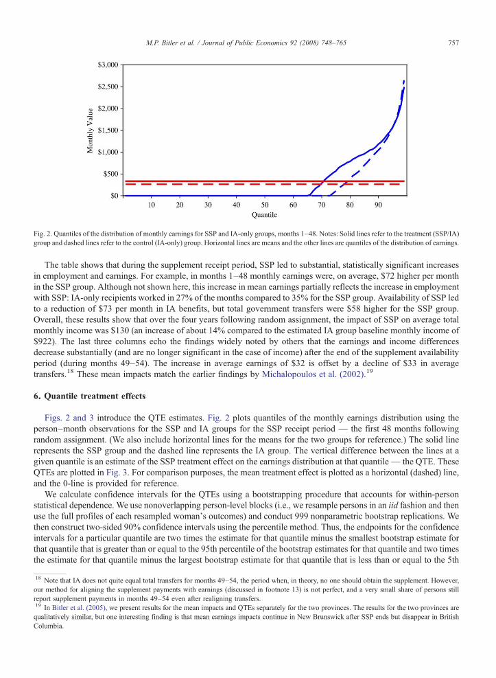
Fig. 2. Quantiles of the distribution of monthly earnings for SSP and IA-only groups, months 1–48. Notes: Solid lines refer to the treatment (SSP/IA)group and dashed lines refer to the control (IA-only) group. Horizontal lines are means and the other lines are quantiles of the distribution of earnings.


The table shows that during the supplement receipt period, SSP led to substantial, statistically significant increasesin employment and earnings. For example, in months 1–48 monthly earnings were, on average, $72 higher per monthin the SSP group. Although not shown here, this increase in mean earnings partially reflects the increase in employmentwith SSP: IA-only recipients worked in 27% of the months compared to 35% for the SSP group. Availability of SSP ledto a reduction of $73 per month in IA benefits, but total government transfers were $58 higher for the SSP group.Overall, these results show that over the four years following random assignment, the impact of SSP on average totalmonthly income was $130 (an increase of about 14% compared to the estimated IA group baseline monthly income of$922). The last three columns echo the findings widely noted by others that the earnings and income differencesdecrease substantially (and are no longer significant in the case of income) after the end of the supplement availabilityperiod (during months 49–54). The increase in average earnings of $32 is offset by a decline of $33 in averagetransfers.18 These mean impacts match the earlier findings by Michalopoulos et al. (2002).19

6. Quantile treatment effects

Figs. 2 and 3 introduce the QTE estimates. Fig. 2 plots quantiles of the monthly earnings distribution using theperson–month observations for the SSP and IA groups for the SSP receipt period — the first 48 months followingrandom assignment. (We also include horizontal lines for the means for the two groups for reference.) The solid linerepresents the SSP group and the dashed line represents the IA group. The vertical difference between the lines at agiven quantile is an estimate of the SSP treatment effect on the earnings distribution at that quantile— the QTE. TheseQTEs are plotted in Fig. 3. For comparison purposes, the mean treatment effect is plotted as a horizontal (dashed) line,and the 0-line is provided for reference.

We calculate confidence intervals for the QTEs using a bootstrapping procedure that accounts for within-personstatistical dependence. We use nonoverlapping person-level blocks (i.e., we resample persons in an iid fashion and thenuse the full profiles of each resampled woman's outcomes) and conduct 999 nonparametric bootstrap replications. Wethen construct two-sided 90% confidence intervals using the percentile method. Thus, the endpoints for the confidenceintervals for a particular quantile are two times the estimate for that quantile minus the smallest bootstrap estimate forthat quantile that is greater than or equal to the 95th percentile of the bootstrap estimates for that quantile and two timesthe estimate for that quantile minus the largest bootstrap estimate for that quantile that is less than or equal to the 5th

18 Note that IA does not quite equal total transfers for months 49–54, the period when, in theory, no one should obtain the supplement. However,our method for aligning the supplement payments with earnings (discussed in footnote 13) is not perfect, and a very small share of persons stillreport supplement payments in months 49–54 even after realigning transfers.19 In Bitler et al. (2005), we present results for the mean impacts and QTEs separately for the two provinces. The results for the two provinces arequalitatively similar, but one interesting finding is that mean earnings impacts continue in New Brunswick after SSP ends but disappear in BritishColumbia.

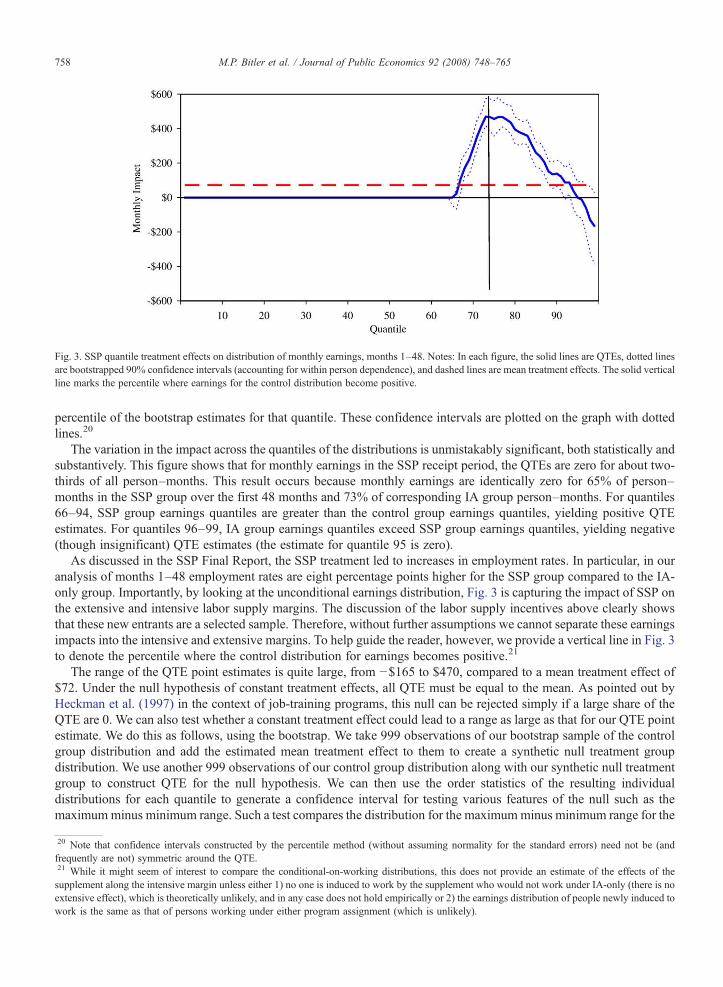
Fig. 3. SSP quantile treatment effects on distribution of monthly earnings, months 1–48. Notes: In each figure, the solid lines are QTEs, dotted linesare bootstrapped 90% confidence intervals (accounting for within person dependence), and dashed lines are mean treatment effects. The solid verticalline marks the percentile where earnings for the control distribution become positive.


percentile of the bootstrap estimates for that quantile. These confidence intervals are plotted on the graph with dottedlines.20

The variation in the impact across the quantiles of the distributions is unmistakably significant, both statistically andsubstantively. This figure shows that for monthly earnings in the SSP receipt period, the QTEs are zero for about two-thirds of all person–months. This result occurs because monthly earnings are identically zero for 65% of person–months in the SSP group over the first 48 months and 73% of corresponding IA group person–months. For quantiles66–94, SSP group earnings quantiles are greater than the control group earnings quantiles, yielding positive QTEestimates. For quantiles 96–99, IA group earnings quantiles exceed SSP group earnings quantiles, yielding negative(though insignificant) QTE estimates (the estimate for quantile 95 is zero).

As discussed in the SSP Final Report, the SSP treatment led to increases in employment rates. In particular, in ouranalysis of months 1–48 employment rates are eight percentage points higher for the SSP group compared to the IA-only group. Importantly, by looking at the unconditional earnings distribution, Fig. 3 is capturing the impact of SSP onthe extensive and intensive labor supply margins. The discussion of the labor supply incentives above clearly showsthat these new entrants are a selected sample. Therefore, without further assumptions we cannot separate these earningsimpacts into the intensive and extensive margins. To help guide the reader, however, we provide a vertical line in Fig. 3to denote the percentile where the control distribution for earnings becomes positive.21

The range of the QTE point estimates is quite large, from −$165 to $470, compared to a mean treatment effect of$72. Under the null hypothesis of constant treatment effects, all QTE must be equal to the mean. As pointed out byHeckman et al. (1997) in the context of job-training programs, this null can be rejected simply if a large share of theQTE are 0. We can also test whether a constant treatment effect could lead to a range as large as that for our QTE pointestimate. We do this as follows, using the bootstrap. We take 999 observations of our bootstrap sample of the controlgroup distribution and add the estimated mean treatment effect to them to create a synthetic null treatment groupdistribution. We use another 999 observations of our control group distribution along with our synthetic null treatmentgroup to construct QTE for the null hypothesis. We can then use the order statistics of the resulting individualdistributions for each quantile to generate a confidence interval for testing various features of the null such as themaximumminus minimum range. Such a test compares the distribution for the maximumminus minimum range for the

20 Note that confidence intervals constructed by the percentile method (without assuming normality for the standard errors) need not be (andfrequently are not) symmetric around the QTE.21 While it might seem of interest to compare the conditional-on-working distributions, this does not provide an estimate of the effects of thesupplement along the intensive margin unless either 1) no one is induced to work by the supplement who would not work under IA-only (there is noextensive effect), which is theoretically unlikely, and in any case does not hold empirically or 2) the earnings distribution of people newly induced towork is the same as that of persons working under either program assignment (which is unlikely).

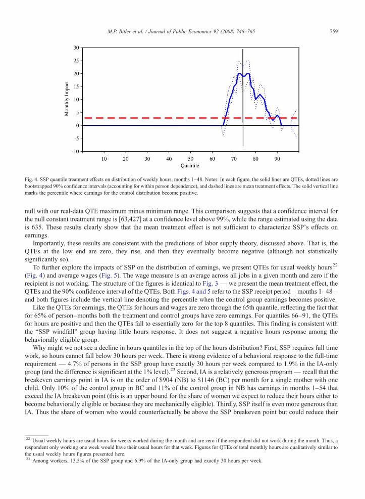
Fig. 4. SSP quantile treatment effects on distribution of weekly hours, months 1–48. Notes: In each figure, the solid lines are QTEs, dotted lines arebootstrapped 90% confidence intervals (accounting for within person dependence), and dashed lines are mean treatment effects. The solid vertical linemarks the percentile where earnings for the control distribution become positive.


null with our real-data QTE maximum minus minimum range. This comparison suggests that a confidence interval forthe null constant treatment range is [63,427] at a confidence level above 99%, while the range estimated using the datais 635. These results clearly show that the mean treatment effect is not sufficient to characterize SSP's effects onearnings.

Importantly, these results are consistent with the predictions of labor supply theory, discussed above. That is, theQTEs at the low end are zero, they rise, and then they eventually become negative (although not statisticallysignificantly so).

To further explore the impacts of SSP on the distribution of earnings, we present QTEs for usual weekly hours22

(Fig. 4) and average wages (Fig. 5). The wage measure is an average across all jobs in a given month and zero if therecipient is not working. The structure of the figures is identical to Fig. 3 — we present the mean treatment effect, theQTEs and the 90% confidence interval of the QTEs. Both Figs. 4 and 5 refer to the SSP receipt period –months 1–48 –and both figures include the vertical line denoting the percentile when the control group earnings becomes positive.

Like the QTEs for earnings, the QTEs for hours and wages are zero through the 65th quantile, reflecting the fact thatfor 65% of person–months both the treatment and control groups have zero earnings. For quantiles 66–91, the QTEsfor hours are positive and then the QTEs fall to essentially zero for the top 8 quantiles. This finding is consistent withthe “SSP windfall” group having little hours response. It does not suggest a negative hours response among thebehaviorally eligible group.

Why might we not see a decline in hours quantiles in the top of the hours distribution? First, SSP requires full timework, so hours cannot fall below 30 hours per week. There is strong evidence of a behavioral response to the full-timerequirement — 4.7% of persons in the SSP group have exactly 30 hours per week compared to 1.9% in the IA-onlygroup (and the difference is significant at the 1% level).23 Second, IA is a relatively generous program— recall that thebreakeven earnings point in IA is on the order of $904 (NB) to $1146 (BC) per month for a single mother with onechild. Only 10% of the control group in BC and 11% of the control group in NB has earnings in months 1–54 thatexceed the IA breakeven point (this is an upper bound for the share of women we expect to reduce their hours either tobecome behaviorally eligible or because they are mechanically eligible). Thirdly, SSP itself is even more generous thanIA. Thus the share of women who would counterfactually be above the SSP breakeven point but could reduce their

22 Usual weekly hours are usual hours for weeks worked during the month and are zero if the respondent did not work during the month. Thus, arespondent only working one week would have their usual hours for that week. Figures for QTEs of total monthly hours are qualitatively similar tothe usual weekly hours figures presented here.23 Among workers, 13.5% of the SSP group and 6.9% of the IA-only group had exactly 30 hours per week.

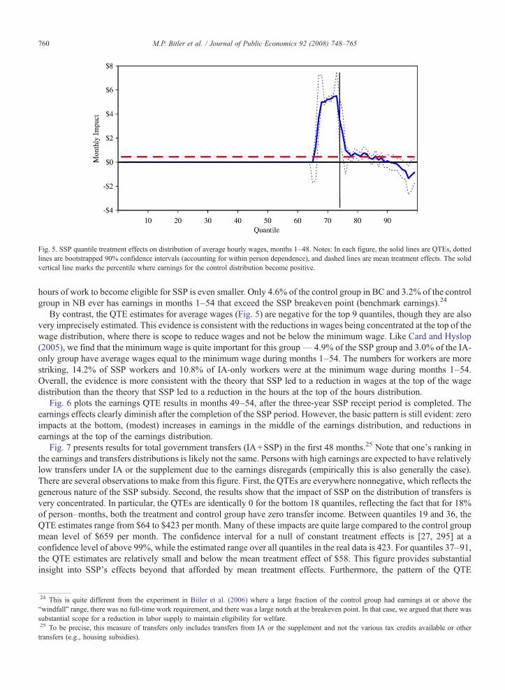
Fig. 5. SSP quantile treatment effects on distribution of average hourly wages, months 1–48. Notes: In each figure, the solid lines are QTEs, dottedlines are bootstrapped 90% confidence intervals (accounting for within person dependence), and dashed lines are mean treatment effects. The solidvertical line marks the percentile where earnings for the control distribution become positive.


hours of work to become eligible for SSP is even smaller. Only 4.6% of the control group in BC and 3.2% of the controlgroup in NB ever has earnings in months 1–54 that exceed the SSP breakeven point (benchmark earnings).24

By contrast, the QTE estimates for average wages (Fig. 5) are negative for the top 9 quantiles, though they are alsovery imprecisely estimated. This evidence is consistent with the reductions in wages being concentrated at the top of thewage distribution, where there is scope to reduce wages and not be below the minimum wage. Like Card and Hyslop(2005), we find that the minimum wage is quite important for this group— 4.9% of the SSP group and 3.0% of the IA-only group have average wages equal to the minimum wage during months 1–54. The numbers for workers are morestriking, 14.2% of SSP workers and 10.8% of IA-only workers were at the minimum wage during months 1–54.Overall, the evidence is more consistent with the theory that SSP led to a reduction in wages at the top of the wagedistribution than the theory that SSP led to a reduction in the hours at the top of the hours distribution.

Fig. 6 plots the earnings QTE results in months 49–54, after the three-year SSP receipt period is completed. Theearnings effects clearly diminish after the completion of the SSP period. However, the basic pattern is still evident: zeroimpacts at the bottom, (modest) increases in earnings in the middle of the earnings distribution, and reductions inearnings at the top of the earnings distribution.

Fig. 7 presents results for total government transfers (IA+SSP) in the first 48 months.25 Note that one's ranking inthe earnings and transfers distributions is likely not the same. Persons with high earnings are expected to have relativelylow transfers under IA or the supplement due to the earnings disregards (empirically this is also generally the case).There are several observations to make from this figure. First, the QTEs are everywhere nonnegative, which reflects thegenerous nature of the SSP subsidy. Second, the results show that the impact of SSP on the distribution of transfers isvery concentrated. In particular, the QTEs are identically 0 for the bottom 18 quantiles, reflecting the fact that for 18%of person–months, both the treatment and control group have zero transfer income. Between quantiles 19 and 36, theQTE estimates range from $64 to $423 per month. Many of these impacts are quite large compared to the control groupmean level of $659 per month. The confidence interval for a null of constant treatment effects is [27, 295] at aconfidence level of above 99%, while the estimated range over all quantiles in the real data is 423. For quantiles 37–91,the QTE estimates are relatively small and below the mean treatment effect of $58. This figure provides substantialinsight into SSP's effects beyond that afforded by mean treatment effects. Furthermore, the pattern of the QTE

24 This is quite different from the experiment in Bitler et al. (2006) where a large fraction of the control group had earnings at or above the“windfall” range, there was no full-time work requirement, and there was a large notch at the breakeven point. In that case, we argued that there wassubstantial scope for a reduction in labor supply to maintain eligibility for welfare.25 To be precise, this measure of transfers only includes transfers from IA or the supplement and not the various tax credits available or othertransfers (e.g., housing subsidies).

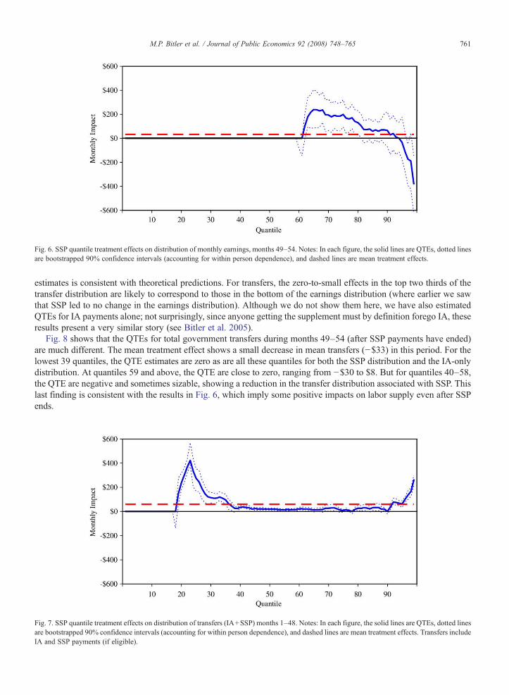
Fig. 6. SSP quantile treatment effects on distribution of monthly earnings, months 49–54. Notes: In each figure, the solid lines are QTEs, dotted linesare bootstrapped 90% confidence intervals (accounting for within person dependence), and dashed lines are mean treatment effects.


estimates is consistent with theoretical predictions. For transfers, the zero-to-small effects in the top two thirds of thetransfer distribution are likely to correspond to those in the bottom of the earnings distribution (where earlier we sawthat SSP led to no change in the earnings distribution). Although we do not show them here, we have also estimatedQTEs for IA payments alone; not surprisingly, since anyone getting the supplement must by definition forego IA, theseresults present a very similar story (see Bitler et al. 2005).

Fig. 8 shows that the QTEs for total government transfers during months 49–54 (after SSP payments have ended)are much different. The mean treatment effect shows a small decrease in mean transfers (−$33) in this period. For thelowest 39 quantiles, the QTE estimates are zero as are all these quantiles for both the SSP distribution and the IA-onlydistribution. At quantiles 59 and above, the QTE are close to zero, ranging from −$30 to $8. But for quantiles 40–58,the QTE are negative and sometimes sizable, showing a reduction in the transfer distribution associated with SSP. Thislast finding is consistent with the results in Fig. 6, which imply some positive impacts on labor supply even after SSPends.

Fig. 7. SSP quantile treatment effects on distribution of transfers (IA+SSP) months 1–48. Notes: In each figure, the solid lines are QTEs, dotted linesare bootstrapped 90% confidence intervals (accounting for within person dependence), and dashed lines are mean treatment effects. Transfers includeIA and SSP payments (if eligible).

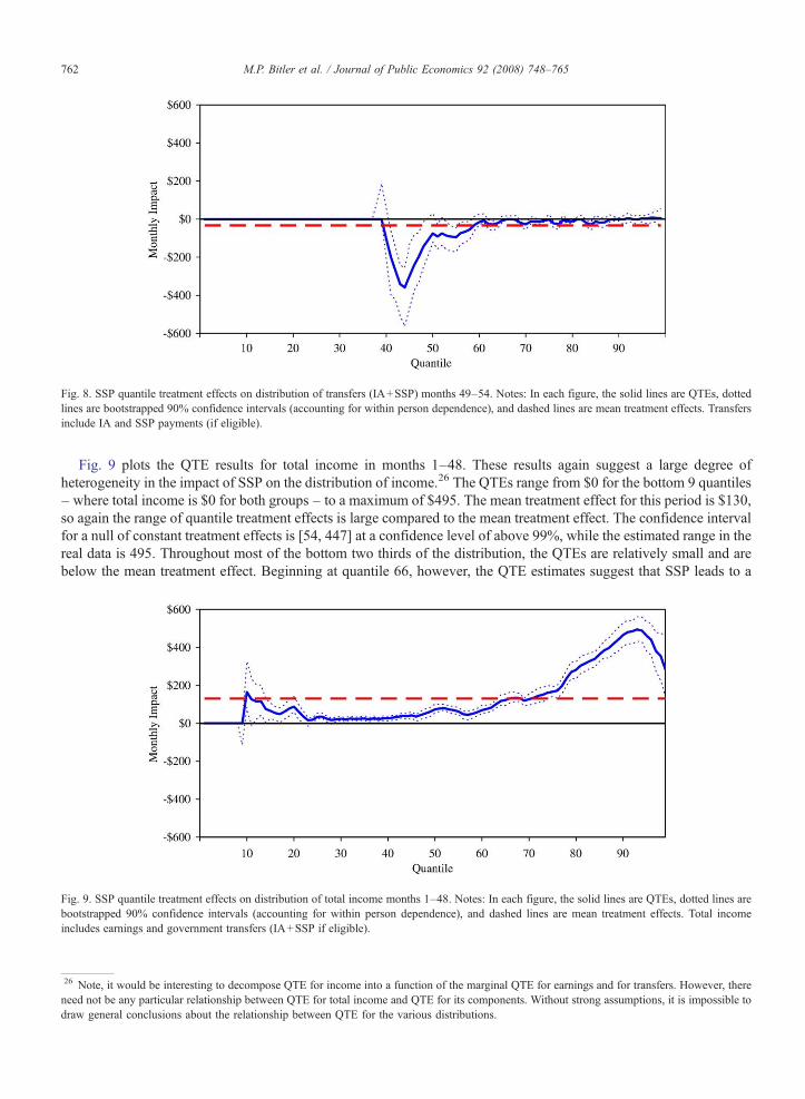
Fig. 8. SSP quantile treatment effects on distribution of transfers (IA+SSP) months 49–54. Notes: In each figure, the solid lines are QTEs, dottedlines are bootstrapped 90% confidence intervals (accounting for within person dependence), and dashed lines are mean treatment effects. Transfersinclude IA and SSP payments (if eligible).


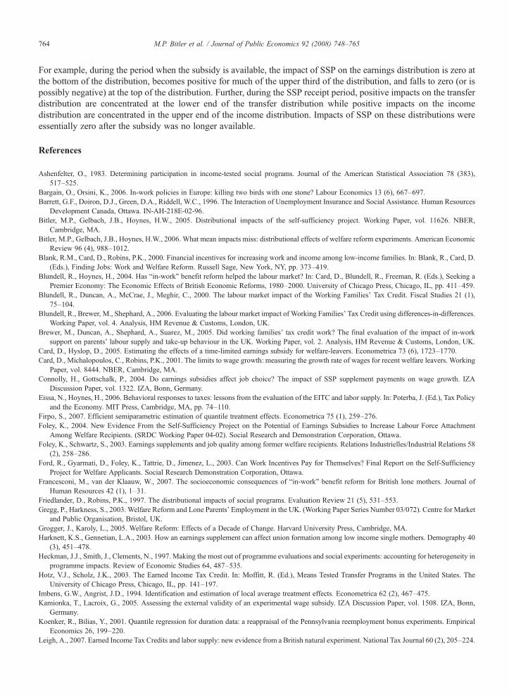
Fig. 9 plots the QTE results for total income in months 1–48. These results again suggest a large degree ofheterogeneity in the impact of SSP on the distribution of income.26 The QTEs range from $0 for the bottom 9 quantiles– where total income is $0 for both groups – to a maximum of $495. The mean treatment effect for this period is $130,so again the range of quantile treatment effects is large compared to the mean treatment effect. The confidence intervalfor a null of constant treatment effects is [54, 447] at a confidence level of above 99%, while the estimated range in thereal data is 495. Throughout most of the bottom two thirds of the distribution, the QTEs are relatively small and arebelow the mean treatment effect. Beginning at quantile 66, however, the QTE estimates suggest that SSP leads to a

Fig. 9. SSP quantile treatment effects on distribution of total income months 1–48. Notes: In each figure, the solid lines are QTEs, dotted lines arebootstrapped 90% confidence intervals (accounting for within person dependence), and dashed lines are mean treatment effects. Total incomeincludes earnings and government transfers (IA+SSP if eligible).

26 Note, it would be interesting to decompose QTE for income into a function of the marginal QTE for earnings and for transfers. However, thereneed not be any particular relationship between QTE for total income and QTE for its components. Without strong assumptions, it is impossible todraw general conclusions about the relationship between QTE for the various distributions.

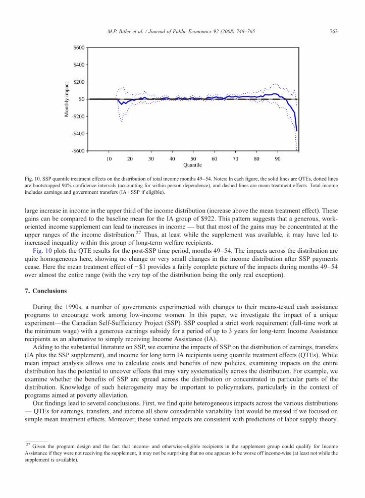
Fig. 10. SSP quantile treatment effects on the distribution of total income months 49–54. Notes: In each figure, the solid lines are QTEs, dotted linesare bootstrapped 90% confidence intervals (accounting for within person dependence), and dashed lines are mean treatment effects. Total incomeincludes earnings and government transfers (IA+SSP if eligible).


large increase in income in the upper third of the income distribution (increase above the mean treatment effect). Thesegains can be compared to the baseline mean for the IA group of $922. This pattern suggests that a generous, work-oriented income supplement can lead to increases in income — but that most of the gains may be concentrated at theupper ranges of the income distribution.27 Thus, at least while the supplement was available, it may have led toincreased inequality within this group of long-term welfare recipients.

Fig. 10 plots the QTE results for the post-SSP time period, months 49–54. The impacts across the distribution arequite homogeneous here, showing no change or very small changes in the income distribution after SSP paymentscease. Here the mean treatment effect of −$1 provides a fairly complete picture of the impacts during months 49–54over almost the entire range (with the very top of the distribution being the only real exception).

7. Conclusions

During the 1990s, a number of governments experimented with changes to their means-tested cash assistanceprograms to encourage work among low-income women. In this paper, we investigate the impact of a uniqueexperiment—the Canadian Self-Sufficiency Project (SSP). SSP coupled a strict work requirement (full-time work atthe minimum wage) with a generous earnings subsidy for a period of up to 3 years for long-term Income Assistancerecipients as an alternative to simply receiving Income Assistance (IA).

Adding to the substantial literature on SSP, we examine the impacts of SSP on the distribution of earnings, transfers(IA plus the SSP supplement), and income for long term IA recipients using quantile treatment effects (QTEs). Whilemean impact analysis allows one to calculate costs and benefits of new policies, examining impacts on the entiredistribution has the potential to uncover effects that may vary systematically across the distribution. For example, weexamine whether the benefits of SSP are spread across the distribution or concentrated in particular parts of thedistribution. Knowledge of such heterogeneity may be important to policymakers, particularly in the context ofprograms aimed at poverty alleviation.

Our findings lead to several conclusions. First, we find quite heterogeneous impacts across the various distributions— QTEs for earnings, transfers, and income all show considerable variability that would be missed if we focused onsimple mean treatment effects. Moreover, these varied impacts are consistent with predictions of labor supply theory.

27 Given the program design and the fact that income- and otherwise-eligible recipients in the supplement group could qualify for IncomeAssistance if they were not receiving the supplement, it may not be surprising that no one appears to be worse off income-wise (at least not while thesupplement is available).


For example, during the period when the subsidy is available, the impact of SSP on the earnings distribution is zero atthe bottom of the distribution, becomes positive for much of the upper third of the distribution, and falls to zero (or ispossibly negative) at the top of the distribution. Further, during the SSP receipt period, positive impacts on the transferdistribution are concentrated at the lower end of the transfer distribution while positive impacts on the incomedistribution are concentrated in the upper end of the income distribution. Impacts of SSP on these distributions wereessentially zero after the subsidy was no longer available.

References

Ashenfelter, O., 1983. Determining participation in income-tested social programs. Journal of the American Statistical Association 78 (383),517–525.

Bargain, O., Orsini, K., 2006. In-work policies in Europe: killing two birds with one stone? Labour Economics 13 (6), 667–697.Barrett, G.F., Doiron, D.J., Green, D.A., Riddell, W.C., 1996. The Interaction of Unemployment Insurance and Social Assistance. Human Resources

Development Canada, Ottawa. IN-AH-218E-02-96.Bitler, M.P., Gelbach, J.B., Hoynes, H.W., 2005. Distributional impacts of the self-sufficiency project. Working Paper, vol. 11626. NBER,

Cambridge, MA.Bitler, M.P., Gelbach, J.B., Hoynes, H.W., 2006. What mean impacts miss: distributional effects of welfare reform experiments. American Economic

Review 96 (4), 988–1012.Blank, R.M., Card, D., Robins, P.K., 2000. Financial incentives for increasing work and income among low-income families. In: Blank, R., Card, D.

(Eds.), Finding Jobs: Work and Welfare Reform. Russell Sage, New York, NY, pp. 373–419.Blundell, R., Hoynes, H., 2004. Has “in-work” benefit reform helped the labour market? In: Card, D., Blundell, R., Freeman, R. (Eds.), Seeking a

Premier Economy: The Economic Effects of British Economic Reforms, 1980–2000. University of Chicago Press, Chicago, IL, pp. 411–459.Blundell, R., Duncan, A., McCrae, J., Meghir, C., 2000. The labour market impact of the Working Families' Tax Credit. Fiscal Studies 21 (1),

75–104.Blundell, R., Brewer, M., Shephard, A., 2006. Evaluating the labour market impact of Working Families' Tax Credit using differences-in-differences.

Working Paper, vol. 4. Analysis, HM Revenue & Customs, London, UK.Brewer, M., Duncan, A., Shephard, A., Suarez, M., 2005. Did working families' tax credit work? The final evaluation of the impact of in-work

support on parents' labour supply and take-up behaviour in the UK. Working Paper, vol. 2. Analysis, HM Revenue & Customs, London, UK.Card, D., Hyslop, D., 2005. Estimating the effects of a time-limited earnings subsidy for welfare-leavers. Econometrica 73 (6), 1723–1770.Card, D., Michalopoulos, C., Robins, P.K., 2001. The limits to wage growth: measuring the growth rate of wages for recent welfare leavers. Working

Paper, vol. 8444. NBER, Cambridge, MA.Connolly, H., Gottschalk, P., 2004. Do earnings subsidies affect job choice? The impact of SSP supplement payments on wage growth. IZA

Discussion Paper, vol. 1322. IZA, Bonn, Germany.Eissa, N., Hoynes, H., 2006. Behavioral responses to taxes: lessons from the evaluation of the EITC and labor supply. In: Poterba, J. (Ed.), Tax Policy

and the Economy. MIT Press, Cambridge, MA, pp. 74–110.Firpo, S., 2007. Efficient semiparametric estimation of quantile treatment effects. Econometrica 75 (1), 259–276.Foley, K., 2004. New Evidence From the Self-Sufficiency Project on the Potential of Earnings Subsidies to Increase Labour Force Attachment

Among Welfare Recipients. (SRDC Working Paper 04-02). Social Research and Demonstration Corporation, Ottawa.Foley, K., Schwartz, S., 2003. Earnings supplements and job quality among former welfare recipients. Relations Industrielles/Industrial Relations 58

(2), 258–286.Ford, R., Gyarmati, D., Foley, K., Tattrie, D., Jimenez, L., 2003. Can Work Incentives Pay for Themselves? Final Report on the Self-Sufficiency

Project for Welfare Applicants. Social Research Demonstration Corporation, Ottawa.Francesconi, M., van der Klaauw, W., 2007. The socioeconomic consequences of “in-work” benefit reform for British lone mothers. Journal of

Human Resources 42 (1), 1–31.Friedlander, D., Robins, P.K., 1997. The distributional impacts of social programs. Evaluation Review 21 (5), 531–553.Gregg, P., Harkness, S., 2003. Welfare Reform and Lone Parents' Employment in the UK. (Working Paper Series Number 03/072). Centre for Market

and Public Organisation, Bristol, UK.Grogger, J., Karoly, L., 2005. Welfare Reform: Effects of a Decade of Change. Harvard University Press, Cambridge, MA.Harknett, K.S., Gennetian, L.A., 2003. How an earnings supplement can affect union formation among low income single mothers. Demography 40

(3), 451–478.Heckman, J.J., Smith, J., Clements, N., 1997. Making the most out of programme evaluations and social experiments: accounting for heterogeneity in

programme impacts. Review of Economic Studies 64, 487–535.Hotz, V.J., Scholz, J.K., 2003. The Earned Income Tax Credit. In: Moffitt, R. (Ed.), Means Tested Transfer Programs in the United States. The

University of Chicago Press, Chicago, IL, pp. 141–197.Imbens, G.W., Angrist, J.D., 1994. Identification and estimation of local average treatment effects. Econometrica 62 (2), 467–475.Kamionka, T., Lacroix, G., 2005. Assessing the external validity of an experimental wage subsidy. IZA Discussion Paper, vol. 1508. IZA, Bonn,

Germany.Koenker, R., Bilias, Y., 2001. Quantile regression for duration data: a reappraisal of the Pennsylvania reemployment bonus experiments. Empirical

Economics 26, 199–220.Leigh, A., 2007. Earned Income Tax Credits and labor supply: new evidence from a British natural experiment. National Tax Journal 60 (2), 205–224.


Lise, J., Seitz, S., Smith, J., 2005. Equilibrium policy experiments and the evaluation of social programs. Mimeograph. Kingston, Ontario; Queen'sUniversity.

Michalopoulos, C., Tattrie, D., Miller, C., Robins, P.K., Morris, P., Gyarmati, D., Redcross, C., Foley, K., Ford, D., 2002. Making Work Pay: FinalReport on the Self-Sufficiency Project for Long-term Welfare Recipients. Social Research and Demonstration Corporation.

Michalopoulos, C., Robins, P., Card, D., 2005. When financial work incentives pay for themselves: evidence from a randomized social experiment forwelfare recipients. Journal of Public Economics 89 (1), 5–29.

Owens, J., 2005. Fundamental Tax Reform: The Experience of OECD Countries. Tax Foundation, Washington, DC. Background Paper Number 47.Smith, N., Dex, S., Vlasblom, J., Callan, T., 2003. The effects of taxation on married women's labour supply across four countries. Oxford Economic

Papers 55 (3), 417–439.Wooldridge, J.M., in press. Inverse Probability Weighted Estimation for General Missing Data Problems. Journal of Econometrics.Zabel, J., Schwartz, S., Donald, S., 2006. An Econometric Analysis of the Impact of the Self-Sufficiency Project on Unemployment and Employment

Durations. IZA Discussion Paper, vol. 2122. IZA, Bonn, Germany.

distributional impacts of the self-sufficiency project · distributional impacts of the...

Documents