Working paper

Poverty and Productivity

Small-Scale Farming in Tanzania, 1991-2007

Razack Lokina Måns Nerman Justin Sandefur

April 2011

When citing this paper, please use the title and the following reference number: F-40006-TZA-1

Poverty & Productivity:

Small-Scale Farming in Tanzania, 1991-2007

⇤

Razack Lokina, University of Dar es SalaamMans Nerman, University of Gothenburg

Justin Sandefur, Center for Global Development

April 29, 2011

Abstract

We examine the role of agriculture, and in particular smallholder farming,in economic growth and poverty reduction in Tanzania in the 1990s and 2000s.A large, but steadily declining majority of Tanzanians earned their living fromfarming over this period, and the relative poverty of farm households com-pared to non-farm households actually worsened. Household survey data from1991 to 2007 reveals that occupational shifts away from the agriculture sector– what we refer to as structural change – made a larger contribution to overallconsumption growth than did income growth within agriculture. Within thefarming sector, we find that the very modest gains in maize output, for in-stance, are due entirely to area expansion rather than any increase in averagecrop-level productivity. Reinforcing this point, crop-level production func-tions for 2001 and 2007 indicate strong declines in total factor productivityfor maize. Finally, we use these production-function results to investigate thedeterminants of productivity, and the potential for policies promoting inor-ganic fertilizer and hybrid seeds for staple crops to raise farm productivityand household incomes. These technologies appear profitable on average, buttheir viability is likely to vary with soil conditions and market access, areasmeriting further research.

⇤This paper was commissioned by the International Growth Centre (IGC) Tanzania,www.theigc.org, with funding from the UK Department for International Development (DfID).We are grateful to the National Bureau of Statistics and the Ministry of Industry, Trade and Mar-keting for providing access to data sources, to Trudy Owens for sharing her calculations underlyingthe consumption aggregates for the Household Budget Surveys, and to Christopher Adam, StefanDercon, and Doug Gollin for helpful comments. For further information on the data sources usedhere and o�cial statistics, please contact the Director General, National Bureau of Statistics atdg@nbs.go.tz. The views expressed are solely those of the authors.

1

Contents

1 Introduction 4

2 Data sources 82.1 Household Budget Surveys: 1991/92, 2000, 2007 . . . . . . . . . . . . 82.2 National Sample Census of Agricultural: 2002-03 . . . . . . . . . . . 92.3 National Panel Survey: 2008-09 . . . . . . . . . . . . . . . . . . . . . 102.4 Rainfall data: 2002 - 2008 . . . . . . . . . . . . . . . . . . . . . . . . 10

3 Growth and exit: two roles for agriculture in consumption growth 123.1 Structural change: the decrease in peasant farming . . . . . . . . . . 143.2 Growth within agriculture: falling further behind . . . . . . . . . . . 14

4 Intensive and extensive margins: Sources of output growth withinsmallholder agriculture 194.1 The intensive margin: declining farm yields . . . . . . . . . . . . . . . 214.2 The extensive margin: area expansion and fairly stable cropping pat-

terns . . . . . . . . . . . . . . . . . . . . . . . . . . . . . . . . . . . . 234.3 The farm size–productivity relationship . . . . . . . . . . . . . . . . . 24

5 Technology adoption and TFP 305.1 Empirical model . . . . . . . . . . . . . . . . . . . . . . . . . . . . . . 305.2 Trends in technology adoption . . . . . . . . . . . . . . . . . . . . . . 325.3 Trends in TFP . . . . . . . . . . . . . . . . . . . . . . . . . . . . . . 335.4 Is fertilizer profitable? . . . . . . . . . . . . . . . . . . . . . . . . . . 37

5.4.1 Are adopters & non-adopters comparable? . . . . . . . . . . . 395.4.2 Can new adopters expect the same returns? . . . . . . . . . . 405.4.3 Which crop price is relevant for profitability? . . . . . . . . . . 42

6 Conclusions 53

List of Tables

1 Definitions of Key Variables . . . . . . . . . . . . . . . . . . . . . . . 112 Occupational Shares and Average Consumption, 1991-2007 . . . . . 133 Sources of Crop Output Growth: Changes in Yield, Area Planted and

the Size-Productivity Relationship, 2002/03-2008/09 . . . . . . . . . 224 Percent of households using ‘improved’ farming techniques . . . . . . 325 OLS production functions for NPS and NSCA for Maize . . . . . . . 456 OLS production functions for NPS and NSCA for Rice Paddy . . . . 467 OLS production functions for NPS and NSCA for Beans . . . . . . . 478 Returns to Fertilizer Usage: Results from On-Farm Verification in

Tanzania . . . . . . . . . . . . . . . . . . . . . . . . . . . . . . . . . 489 OLS production functions for NPS only: maize, paddy, and beans . . 49

2

10 Physical returns to inorganic fertilizer implied by Cobb-Douglas spec-ification . . . . . . . . . . . . . . . . . . . . . . . . . . . . . . . . . . 50

11 Median sales and consumption prices reported in the NPS . . . . . . 5112 Value-to-cost ratios of fertilizer usage for di↵erent crops and prices . . 52

List of Figures

1 Schematic Structure of the Paper . . . . . . . . . . . . . . . . . . . . 62 Structural Change, 1991-2007: Sector of Occupation in the HBS . . . 163 Consumption Growth by Occupation of Household Head: 1991-2007 . 174 Sources of Consumption Growth, 1991-2007 . . . . . . . . . . . . . . 185 Intensive versus Extensive Growth: Maize . . . . . . . . . . . . . . . 266 Intensive versus Extensive Growth: Paddy . . . . . . . . . . . . . . . 277 Intensive versus Extensive Growth: Sorghum . . . . . . . . . . . . . . 288 Intensive versus Extensive Growth: Beans . . . . . . . . . . . . . . . 29

3

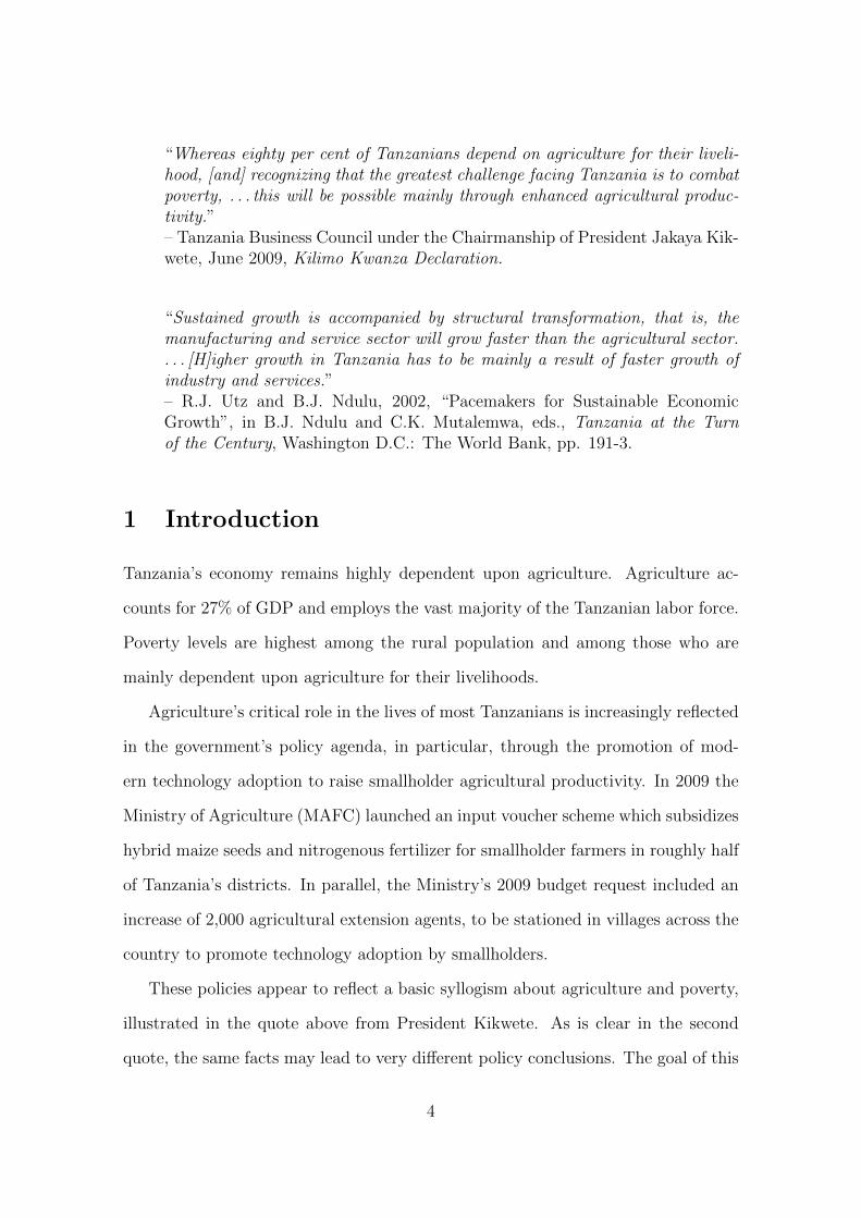
“Whereas eighty per cent of Tanzanians depend on agriculture for their liveli-hood, [and] recognizing that the greatest challenge facing Tanzania is to combatpoverty, . . . this will be possible mainly through enhanced agricultural produc-tivity.”– Tanzania Business Council under the Chairmanship of President Jakaya Kik-wete, June 2009, Kilimo Kwanza Declaration.

“Sustained growth is accompanied by structural transformation, that is, themanufacturing and service sector will grow faster than the agricultural sector.. . . [H]igher growth in Tanzania has to be mainly a result of faster growth ofindustry and services.”– R.J. Utz and B.J. Ndulu, 2002, “Pacemakers for Sustainable EconomicGrowth”, in B.J. Ndulu and C.K. Mutalemwa, eds., Tanzania at the Turnof the Century, Washington D.C.: The World Bank, pp. 191-3.

1 Introduction

Tanzania’s economy remains highly dependent upon agriculture. Agriculture ac-

counts for 27% of GDP and employs the vast majority of the Tanzanian labor force.

Poverty levels are highest among the rural population and among those who are

mainly dependent upon agriculture for their livelihoods.

Agriculture’s critical role in the lives of most Tanzanians is increasingly reflected

in the government’s policy agenda, in particular, through the promotion of mod-

ern technology adoption to raise smallholder agricultural productivity. In 2009 the

Ministry of Agriculture (MAFC) launched an input voucher scheme which subsidizes

hybrid maize seeds and nitrogenous fertilizer for smallholder farmers in roughly half

of Tanzania’s districts. In parallel, the Ministry’s 2009 budget request included an

increase of 2,000 agricultural extension agents, to be stationed in villages across the

country to promote technology adoption by smallholders.

These policies appear to reflect a basic syllogism about agriculture and poverty,

illustrated in the quote above from President Kikwete. As is clear in the second

quote, the same facts may lead to very di↵erent policy conclusions. The goal of this

4

paper is not to advocate one position or the other.1 In either case, the evidence base

necessary to draw firm policy conclusions is woefully lacking.

The goal of this paper is to fill in some of those empirical gaps in the logical

chain from investments in smallholder farm productivity to poverty reduction. We

bring together a wide range of nationally-representative household survey data to

enable comparisons over time. This link between multiple rounds of household and

farm surveys provides, to our knowledge, the most comprehensive picture of small-

scale agricultural development in Tanzania available to date. Parallel work also

commissioned by the International Growth Centre (Kirchberger and Mishili 2011)

will focus on just one of Tanzania’s twenty-one mainland regions, Kagera – for which

more detailed longitudinal household survey data is available – to examine a similar

set of issues.

Figure 1 shows the schematic structure of the paper, which revolves around a

descriptive decomposition of consumption growth over the past two decades into

its various sources. The steps in this decomposition correspond to the outline of

the three main sections of the paper: first examining the role of agricultural in

household consumption growth (Section 3); turning next to the role of yield growth

in agricultural growth (Section 4); and finally investigating the roles of technology

adoption and total-factor productivity (TFP) growth in yield growth (Section 5).

The various stages of this decomposition can be re-phrased in the form of three

empirical questions.

Question 1. Did smallholder productivity growth lift farm households out of poverty?

Or did farmers exit to better opportunities?

In Section 3 we assess the relative importance of these two channels empirically

in recent Tanzanian history. We use household survey data from 1991 to 2007 to

1Indeed, we would argue that these positions are not in fact contradictory, given the potentialrole for agricultural productivity to spur structural change, as emphasized in dual economy models.

5

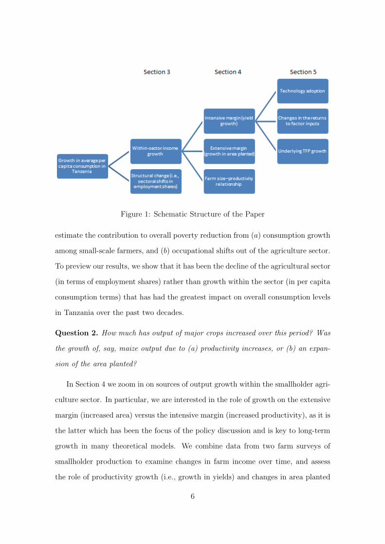
Figure 1: Schematic Structure of the Paper

estimate the contribution to overall poverty reduction from (a) consumption growth

among small-scale farmers, and (b) occupational shifts out of the agriculture sector.

To preview our results, we show that it has been the decline of the agricultural sector

(in terms of employment shares) rather than growth within the sector (in per capita

consumption terms) that has had the greatest impact on overall consumption levels

in Tanzania over the past two decades.

Question 2. How much has output of major crops increased over this period? Was

the growth of, say, maize output due to (a) productivity increases, or (b) an expan-

sion of the area planted?

In Section 4 we zoom in on sources of output growth within the smallholder agri-

culture sector. In particular, we are interested in the role of growth on the extensive

margin (increased area) versus the intensive margin (increased productivity), as it is

the latter which has been the focus of the policy discussion and is key to long-term

growth in many theoretical models. We combine data from two farm surveys of

smallholder production to examine changes in farm income over time, and assess

the role of productivity growth (i.e., growth in yields) and changes in area planted

6

in explaining this income growth. For maize and most other major crops (rice paddy

being the key exception), we find that average yields have actually declined, and

where output growth is present it is primarily attributable to area expansion.

One variable conspicuously absent from this portion of the analysis is crop prices.

We lack comparable data across time (2002-2008) and space (all regions of mainland

Tanzania) on a full set of crops. Thus we are unable to aggregate total output value

across crops or analyze shifts in the terms of trade. Instead we conduct the analysis

separately by crop. We would note that this is one area where the longitudinal

data used by Kirchberger and Mishili (2011) poses the greatest advantage despite

its narrow geographic coverage, in that their survey data enables them to provide

a single, farm-level output measure. Using this measure they document a dramatic

decline of 46% in total crop value from 1991 to 2004 for their Kagera sample.

Question 3. Has use of inorganic fertilizer, hybrid seeds, irrigation, etc. increased?

Why or why not? Are these technologies profitable for smallholders at prevailing

prices?

Finally, in Section 5 we drill down yet another level, focusing on the underlying

determinants of changes in farm yields. We examine changes in the use of improved

farm inputs, and the evolution of the returns to these inputs over time. The latter

task, measuring returns to fertilizer and other inputs, is a much more fraught econo-

metric excercise. Careful alignment of production and input data across two farmer

surveys (from 2002/03 and 2008/09) allows us to estimate a pooled, farm/crop-level

production function. Even so, our results must be treated as correlations rather than

precise evidence of causal parameters. We discuss potential endogeneity problems

that may bias the estimated returns in this section, and compare our results to ex-

perimental (Duflo, Kremer, and Robinson 2009) and longitudinal (Suri 2011) work

on fertilizer returns among maize farmers in neighboring Kenya that has addressed

7

some of these concerns, looking for clues about what this parallel research can tell

us about Tanzania in light of our more descriptive results.

2 Data sources

We draw on three principal data sources. The first is the series of Household Bud-

get Surveys (HBS), conducted in 1991, 2000, and 2007. The HBS surveys are pri-

marily designed to assess household welfare; we use increases in consumption for

smallholder farmers as a first window into trends in agricultural productivity in the

1990s and 2000s, and show how agricultural growth and occupational shifts away

from agriculture have contributed to poverty reduction.

The second and third primary data sources focus on agricultural production

per se. Both are nationally representative, household surveys covering smallholder

farmers. For reasons of comparability we were forced to exclude Zanzibar from the

analysis. While the questionnaires for the two data sources di↵er, they both o↵er

input and output data at the crop level for all major crops, allowing us to estimate

household-level yields and production functions by crop in a comparable way over

time, and to examine changes in cropping patterns and area planted.

2.1 Household Budget Surveys: 1991/92, 2000, 2007

Each round of the HBS is a nationally representative household survey covering all

regions of mainland Tanzania, but not Zanzibar. The primary focus of the HBS is to

measure household consumption, as a basis for poverty measurement. A comparable

consumption aggregate has been compiled for three successive rounds of the HBS,

spanning the period from 1991 to 2007. The basic needs poverty lines which have

been constructed for each geographic stratum (Dar es Salaam, other urban areas,

and rural areas) and each round of the HBS provide an estimate of the cost of

8

acquiring a basic basket of essential food and non-food items. We use these poverty

lines as the basis for deflating nominal consumption figures from each round.

The HBS also includes data on occupational status. We categorize households by

the sector of the main occupation of the household head, which we divided into five

sectors: agriculture, which includes crop farming, livestock and fishing; non-farm

self-employment; wage employment in the public sector, which includes NGOs and

international organizations; wage employment in the private sector which includes

parastatal enterprises; and a category for heads of household who are not working,

which encompasses both the unemployed as well as those outside the labor force.

Our focus here is on the changes in consumption among households engaged in

agriculture, as well as the changes in average consumption due to movements away

from agriculture.

2.2 National Sample Census of Agricultural: 2002-03

The second primary data source is the National Sample Census of Agriculture

(NSCA), 2002-03, conducted by the Ministry of Agriculture, Food Security and

Cooperatives (MAFC) and the National Bureau of Statistics (NBS). The NSCA

includes detailed production data for smallholder farmers, including land area, la-

bor and capital inputs, yields and sales. The sample is large, covering over 48,000

households across 3,200 villages - su�cient to provide district-level estimates for all

of Tanzania. One weakness of the NSCA which should be noted early on is the fairly

coarse treatment of chemical fertilizer, improved seeds, pesticides and herbicides in

the questionnaire. These are asked as binary response questions (used/did not use)

rather than soliciting quantities or prices. (Additionally, the NSCA also includes a

parallel survey of large-scale farmers. We provide basic comparisons between the

smallholder and large-scale farm results, without conducting primary data analysis

on the large farm sample, due to the lack of any comparable data for later time

9

periods as noted below.)

2.3 National Panel Survey: 2008-09

Our third main data source is the baseline round of the National Panel Survey

(NPS), 2008-09, also conducted by NBS with the collaboration of MAFC. The na-

tionally representative sample of the NPS returned to a sub-set of the villages which

participated in the 2002-03 NSCA. (Note this is not a panel of households, only

of villages at this stage.) The NPS sample is relatively small, with approximately

2,000 rural households, but the questionnaire is fairly detailed, and overcomes many

of the weaknesses of the NSCA questionnaire regarding details on input usage and

cost.

2.4 Rainfall data: 2002 - 2008

Finally, to complement the farm and household survey data, we use data from

the Tanzania Meteorological Agency (TMA) measuring monthly rainfall. The TMA

data provides the total millimeters of rainfall from observation points covering nearly

all of Tanzania’s twenty-one mainland regions. Thus we have, roughly speaking,

one rainfall observation per month per region from January 2002 to December 2008

which can be merged with the survey data to control for climate e↵ects in the

determination of farm output in the analysis below.

In order to keep the analysis simple and transparent, our preferred measure of

rainfall is the cumulative millimeters of rainfall (and its square) in a given region for

the months of March, April and May. These months (in 2003 for the NSCA, and

2008 for the NPS) constitute the peak months for the long-rainy season for which

crop output is available. We experiment with more flexible and less parsimonious

rainfall measures to ensure the robustness of the analysis.

10

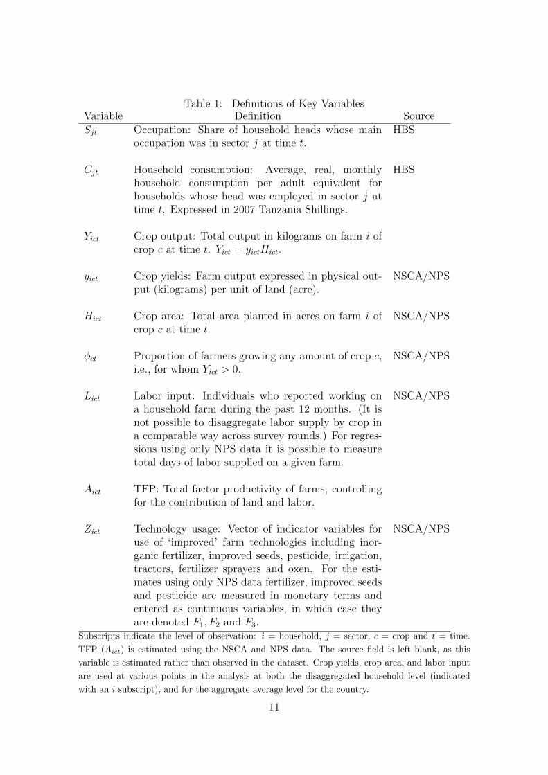
Table 1: Definitions of Key VariablesVariable Definition SourceSjt Occupation: Share of household heads whose main

occupation was in sector j at time t.HBS

Cjt Household consumption: Average, real, monthlyhousehold consumption per adult equivalent forhouseholds whose head was employed in sector j attime t. Expressed in 2007 Tanzania Shillings.

HBS

Yict Crop output: Total output in kilograms on farm i ofcrop c at time t. Yict = yictHict.

yict Crop yields: Farm output expressed in physical out-put (kilograms) per unit of land (acre).

NSCA/NPS

Hict Crop area: Total area planted in acres on farm i ofcrop c at time t.

NSCA/NPS

�ct Proportion of farmers growing any amount of crop c,i.e., for whom Yict > 0.

NSCA/NPS

Lict Labor input: Individuals who reported working ona household farm during the past 12 months. (It isnot possible to disaggregate labor supply by crop ina comparable way across survey rounds.) For regres-sions using only NPS data it is possible to measuretotal days of labor supplied on a given farm.

NSCA/NPS

Aict TFP: Total factor productivity of farms, controllingfor the contribution of land and labor.

Zict Technology usage: Vector of indicator variables foruse of ‘improved’ farm technologies including inor-ganic fertilizer, improved seeds, pesticide, irrigation,tractors, fertilizer sprayers and oxen. For the esti-mates using only NPS data fertilizer, improved seedsand pesticide are measured in monetary terms andentered as continuous variables, in which case theyare denoted F

1

, F2

and F3

.

NSCA/NPS

Subscripts indicate the level of observation: i = household, j = sector, c = crop and t = time.

TFP (Aict) is estimated using the NSCA and NPS data. The source field is left blank, as this

variable is estimated rather than observed in the dataset. Crop yields, crop area, and labor input

are used at various points in the analysis at both the disaggregated household level (indicated

with an i subscript), and for the aggregate average level for the country.

11

Comparing rainfall across the two years, by almost any measure 2008 was a

better year. Averaging over households in the sample the mean cumulative rainfall

from March to April in 2003 was 268 millimeters, rising to 322 millimeters in 2008.

The fifth and ninety-fifth percentiles also rose, from 77 to 196 millimeters and from

664 to 811 millimeters. Looking across the entire year, average rainfall rose for nine

of the twelve months when comparing 2003 to 2008.

3 Growth and exit: two roles for agriculture in

consumption growth

Most Tanzanian households earn their living through farming; to be precise, as

of 1991 the main occupation of 82.1% of household heads was farming, livestock or

fishing. By 2007 his share had fallen to 64.0%. Farm households are also significantly

poorer than other households; in 1991 their real per capita consumption was just

68.6% of the average for non-farm households, and this deficit has widened over time

to just 62.6% by 2007.

In a purely arithmetical sense, the concentration of poor households in the agri-

cultural sector suggests two paths to poverty reduction in Tanzania: consumption

growth among smallholder farmers, and structural change, i.e., movement out of

agriculture into other sectors where average consumption is higher. The HBS data

sets allow us to disentangle the relative importance of these channels in overall con-

sumption growth, as well as the role of consumption growth in other sectors outside

of agriculture.

We begin with a simple decomposition of overall average consumption levels:

Ct =X

j

SjtCjt (1)

12

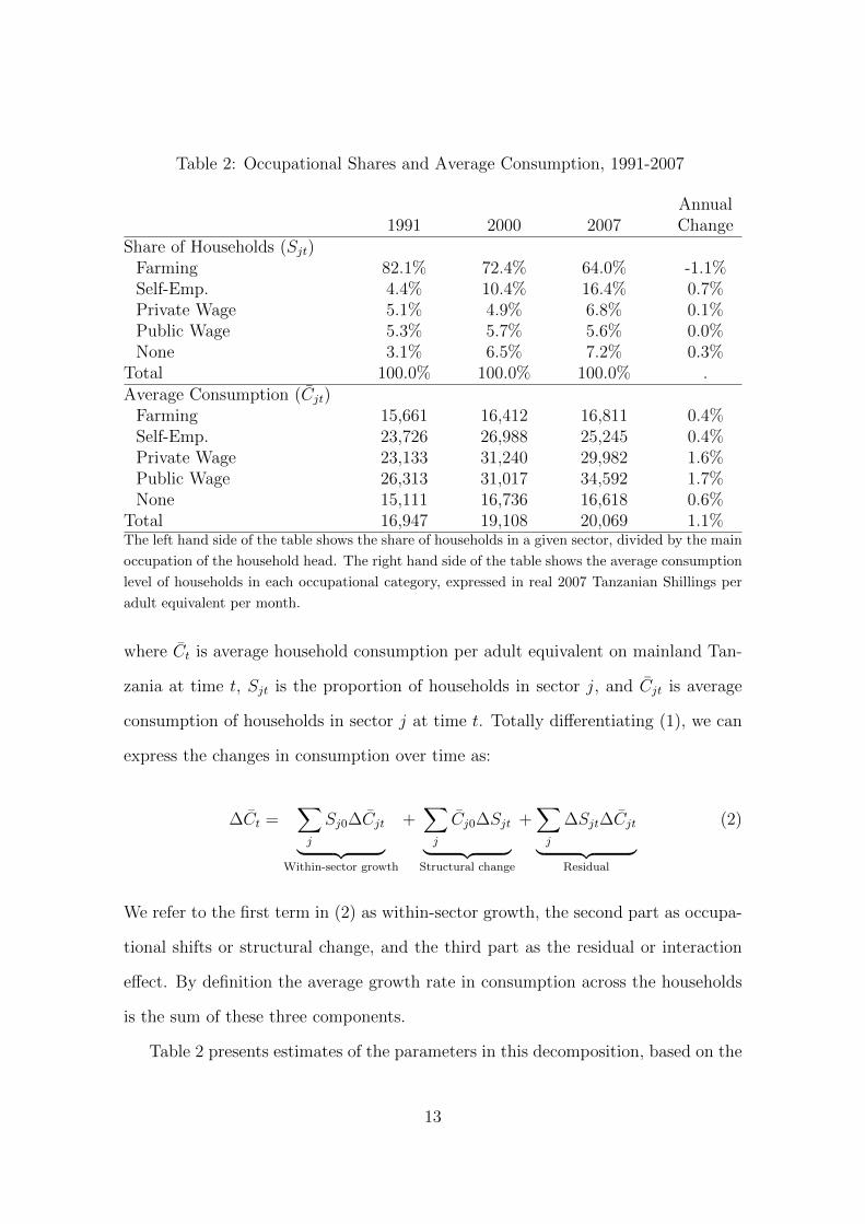
Table 2: Occupational Shares and Average Consumption, 1991-2007

Annual1991 2000 2007 Change

Share of Households (Sjt)Farming 82.1% 72.4% 64.0% -1.1%Self-Emp. 4.4% 10.4% 16.4% 0.7%Private Wage 5.1% 4.9% 6.8% 0.1%Public Wage 5.3% 5.7% 5.6% 0.0%None 3.1% 6.5% 7.2% 0.3%

Total 100.0% 100.0% 100.0% .Average Consumption (Cjt)Farming 15,661 16,412 16,811 0.4%Self-Emp. 23,726 26,988 25,245 0.4%Private Wage 23,133 31,240 29,982 1.6%Public Wage 26,313 31,017 34,592 1.7%None 15,111 16,736 16,618 0.6%

Total 16,947 19,108 20,069 1.1%The left hand side of the table shows the share of households in a given sector, divided by the main

occupation of the household head. The right hand side of the table shows the average consumption

level of households in each occupational category, expressed in real 2007 Tanzanian Shillings per

adult equivalent per month.

where Ct is average household consumption per adult equivalent on mainland Tan-

zania at time t, Sjt is the proportion of households in sector j, and Cjt is average

consumption of households in sector j at time t. Totally di↵erentiating (1), we can

express the changes in consumption over time as:

�Ct =X

j

Sj0�Cjt

| {z }Within-sector growth

+X

j

Cj0�Sjt

| {z }Structural change

+X

j

�Sjt�Cjt

| {z }Residual

(2)

We refer to the first term in (2) as within-sector growth, the second part as occupa-

tional shifts or structural change, and the third part as the residual or interaction

e↵ect. By definition the average growth rate in consumption across the households

is the sum of these three components.

Table 2 presents estimates of the parameters in this decomposition, based on the

13

five occupation categories described in Section 2.1. The top panel shows shifts in the

occupational structure over time. Households are classified into sectors based on the

main occupation of the household head. The bottom panel shows average levels of

monthly household consumption per adult equivalent for households in each sector.

All figures are expressed in real 2007 Tanzanian Shillings, deflated using the o�cial

basic needs poverty lines published by the National Bureau of Statistics. The main

messages from Table 2 are summarized in Figures 2 through 4.

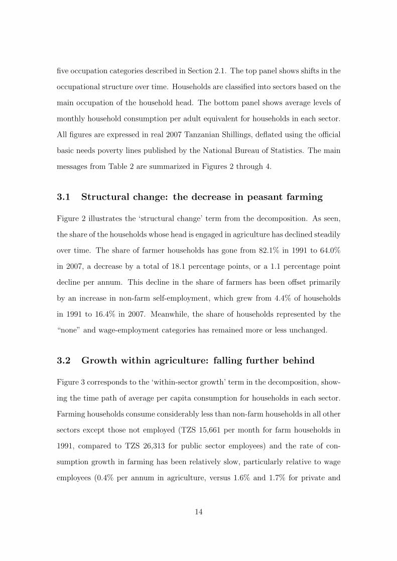
3.1 Structural change: the decrease in peasant farming

Figure 2 illustrates the ‘structural change’ term from the decomposition. As seen,

the share of the households whose head is engaged in agriculture has declined steadily

over time. The share of farmer households has gone from 82.1% in 1991 to 64.0%

in 2007, a decrease by a total of 18.1 percentage points, or a 1.1 percentage point

decline per annum. This decline in the share of farmers has been o↵set primarily

by an increase in non-farm self-employment, which grew from 4.4% of households

in 1991 to 16.4% in 2007. Meanwhile, the share of households represented by the

“none” and wage-employment categories has remained more or less unchanged.

3.2 Growth within agriculture: falling further behind

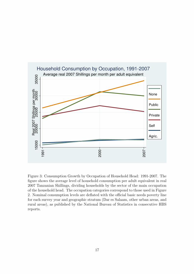
Figure 3 corresponds to the ‘within-sector growth’ term in the decomposition, show-

ing the time path of average per capita consumption for households in each sector.

Farming households consume considerably less than non-farm households in all other

sectors except those not employed (TZS 15,661 per month for farm households in

1991, compared to TZS 26,313 for public sector employees) and the rate of con-

sumption growth in farming has been relatively slow, particularly relative to wage

employees (0.4% per annum in agriculture, versus 1.6% and 1.7% for private and

14

public wage employees, respectively). This means that from 1991 to 2007 the per

capita consumption increased by 5% in the farming sector, compared to 30% and

31% in the private and public wage sectors respectively.

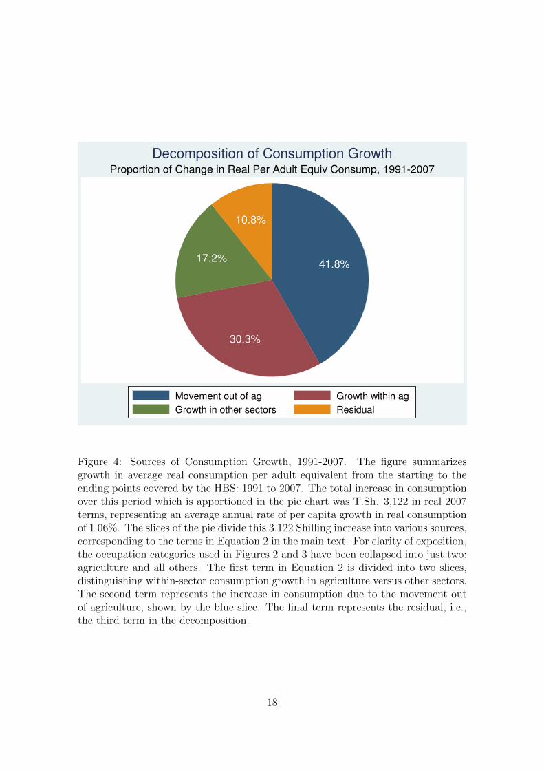
Finally, Figure 4 summarizes the decomposition of total consumption growth

given in Equation 2. Rather than attempting to graph the movements for all five

sectors, we collapse the sectors into just two: farming and other. The slices of pie

chart show the share of total consumption growth attributable to each of the three

main terms of the decomposition. We split the ‘within-sector growth’ term into

two parts, however, to highlight the separate contributions of growth within agri-

culture and within other sectors. This yields a total of four shares. The largest of

these, accounting for 41.8% of total consumption growth is the occupation shift of

households out of agriculture and into other sectors. Growth within agriculture –

although slower than growth in other sectors – accounts for 30.3% of total consump-

tion growth, due to the large initial size of the sector, while growth in other sectors

accounts for just 17.2% of overall consumption growth. Finally, the residual term

accounts for the remaining 10.8% of consumption growth.

15

0.2

.4.6

.81

% o

f H

ouse

hold

s

1991 2000 2007

Occupation of Household Heads, 1991-2007

None

Public

Private

Self

Agric.

Figure 2: Structural Change, 1991-2007: Sector of Occupation in the HBS. Thefigure shows the sector of the main occupation of the household head across threerounds of the HBS, in 1991, 2000 and 2007, covering mainland Tanzania. “Agri-culture” includes crop farming, livestock and fishing. “Self” refers to non-farmself-employment. “Public” and “Private” refer to wage employment in the publicand private sectors, respectively, where parastatal enterprises are included in theprivate category. “None” encompasses both the unemployed as well as those out-side the labor force. As seen, the share of the households whose head is engagedin agriculture has declined steadily over time, o↵set primarily by an increase innon-farm self-employment. The share of households represented by the “none” andwage-employment categories has remained more or less unchanged.

16

15000

20000

25000

30000

35000

Real 2

007 S

hill

ings

per

month

1991

2000

2007

None

Public

Private

Self

Agric.

Average real 2007 Shillings per month per adult equivalent

Household Consumption by Occupation, 1991-2007

Figure 3: Consumption Growth by Occupation of Household Head: 1991-2007. Thefigure shows the average level of household consumption per adult equivalent in real2007 Tanzanian Shillings, dividing households by the sector of the main occupationof the household head. The occupation categories correspond to those used in Figure2. Nominal consumption levels are deflated with the o�cial basic needs poverty linefor each survey year and geographic stratum (Dar es Salaam, other urban areas, andrural areas), as published by the National Bureau of Statistics in consecutive HBSreports.

17

41.8%

30.3%

17.2%

10.8%

Movement out of ag Growth within ag

Growth in other sectors Residual

Proportion of Change in Real Per Adult Equiv Consump, 1991-2007

Decomposition of Consumption Growth

Figure 4: Sources of Consumption Growth, 1991-2007. The figure summarizesgrowth in average real consumption per adult equivalent from the starting to theending points covered by the HBS: 1991 to 2007. The total increase in consumptionover this period which is apportioned in the pie chart was T.Sh. 3,122 in real 2007terms, representing an average annual rate of per capita growth in real consumptionof 1.06%. The slices of the pie divide this 3,122 Shilling increase into various sources,corresponding to the terms in Equation 2 in the main text. For clarity of exposition,the occupation categories used in Figures 2 and 3 have been collapsed into just two:agriculture and all others. The first term in Equation 2 is divided into two slices,distinguishing within-sector consumption growth in agriculture versus other sectors.The second term represents the increase in consumption due to the movement outof agriculture, shown by the blue slice. The final term represents the residual, i.e.,the third term in the decomposition.

18

4 Intensive and extensive margins: Sources of out-

put growth within smallholder agriculture

The previous section looked at how much of the actual consumption growth achieved

in Tanzania has been due to increases in consumption for households in the agri-

cultural sector. This section drills down one step further, to look at the sources of

that growth. To do so requires that we shift focus from consumption to produc-

tion, and decompose output growth into its various components: expansion in the

area planted, growth in farm yields, and changes in the correlation between these

variables – i.e., the farm-size productivity relationship.

Ideally this analysis could be conducted both at the aggregate farm level, and by

disaggregated crops. Aggregating production at the farm level requires crop prices

that are comparable across time. While limited price data is available from the

Ministry of Industry, Trade and Marketing (MITM) it is lacking in several respects:

key crops such as paddy are missing; data is measured at markets rather than the

farm gate, so may not reflect true returns to farmers; etc. At this time we present

analysis exclusively at the individual crop level, and side-step all price calculations.

Readers should keep in mind that changes in income (an intermediate step between

production, as measured here, and consumption dealt with in the previous section)

may also reflect price variation not measured here. Indeed, Kirchberger and Mishili

(2011) observed declining terms of trade between 1991 and 2004 for farmers in the

Kagera region in Tanzania. Such a change may a↵ect farmers’ incomes negatively,

which may play a role in explaining the slow growth of per capita consumption found

within that sector.

Total farm output of crop c in time t on farm i, Yict, is the product farm yields

expressed in physical output per unit of land, yict, and total area planted for a

given crop, Hict. Decomposing output into yield and area planted requires careful

19

attention to the proportion of farms who plant zero maize, for instance, and thus

have no yield data. We use Yct to refer to average output of c, averaging across all

farms – regardless of whether they planted any c. When referring to the average

level of yield or area planted however, (denoted yct and Hct, respectively) we use

only those observations with positive output. We use �ct to denote the proportion

of farmers planting any of crop c in period t. Using this notation and the properties

of expectations, we can write:

Yict = yictHict

) Yct = �ct[yctHct + cov(yict, Hict)] (3)

The term inside the square brackets is equivalent to the average output of farms

that produce any of crop c. This is multiplied by �ct, the share of all farms growing

any of crop c, making the expression as a whole a measure of total output averaged

over all farms. Once again, totally di↵erentiating 3 provides a useful decomposition

of total changes in farm output into the changes of each of these underlying parts:

�Yct = �c0yc0�Hct +��ct[yctHct + cov(yict, Hict)]| {z }Extensive margin

+

�c0�yc0Hct| {z }Intensive margin

+ �c0�cov(yict, Hict)| {z }Size-productivity rel’n

+ "ic (4)

The first two terms show the change in revenue due to expansion of the area planted,

which we refer to as growth along the ‘extensive margin’. The first of these terms

captures the change in the average area planted among households cultivating any

of crop c, as captured by �Hct, and the second term shows the change in the share

of all households that cultivate crop c, as captured by the ��ct parameter. The

third term shows the change in revenue driven by increases in crop yields, which

we refer to as growth along the ‘intensive margin’, and the fourth term shows the

20

e↵ect of changes in the covariance of area and yield, which we refer to as the ‘farm

size–productivity relationship’. All of these terms individually rely on the other

parameters remaining unchanged. For instance, the first term shows the change in

revenue due to changes in the average area planted among cultivating households

– as we stated above – only insofar as the share of households cultivating crop c

and their average yields remain stable. As it is unlikely that these remain exactly

unchanged, there is also a (relatively small) residual term, "ic, which consists of the

cross-products in the total derivative.2

Our data for these calculations is based on the household surveys of smallholder

farmers conducted in 2002/03 and 2008/09, i.e., the NSCA and NPS, respectively.

These surveys e↵ectively provide data on farm production; in contrast the previous

section focused on consumption. While consumption is a more appropriate metric

of household welfare, production data enables us to examine the sources of welfare

gains and relate them to underlying economic activities.

4.1 The intensive margin: declining farm yields

Comparing columns (1) and (2) in Table 3 provides an indication of the relative

importance of yield growth in total output growth for various crops at the national

level, over the time period from 2002/03 to 2008/09.

The overall picture in Table 3 is one of gradually declining yields. Staring with

maize in the upper left corner of the Table, average production among maize farmers

in column (1) grew from 405 kg to 427 kg over this period, reflecting an increase of

21.2 kg over six years, or an annual growth rate in output of just 0.9% per annum.

2To be explicit, the residual term is " = �c0�yct�Hct+��ct[�yctHc0+ yc0�Hct+�yct�Hct+�cov(yct, Hct)]. As seen, these terms are ‘second order’ in the sense that they are the productof changes. Normalizing yields and land area to unity at time zero, it is easy to see that theirmagnitude will be quite small for realistic growth rates in the underlying variables. Thus the four-part decomposition in equation 4 provides a fairly comprehensive picture of the source of outputgrowth.

21

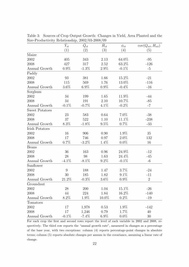
Table 3: Sources of Crop Output Growth: Changes in Yield, Area Planted and theSize-Productivity Relationship, 2002/03-2008/09

Yct Qct Hct �ct cov(Qict, Hict)(1) (2) (3) (4) (5)

Maize2002 405 343 2.13 64.0% -952008 427 317 2.52 63.2% -126Annual Growth 0.9% -1.3% 2.9% -0.1% -5Paddy2002 93 381 1.66 15.2% -212008 115 569 1.76 13.0% -116Annual Growth 3.6% 6.9% 0.9% -0.4% -16Sorghum2002 34 199 1.65 11.9% -442008 34 191 2.10 10.7% -85Annual Growth -0.1% -0.7% 4.1% -0.2% -7Sweet Potatoes2002 23 583 0.64 7.0% -382008 37 522 1.10 11.1% -238Annual Growth 8.3% -1.8% 9.5% 0.7% -33Irish Potatoes2002 16 906 0.90 1.9% 352008 17 746 0.97 2.0% 132Annual Growth 0.7% -3.2% 1.4% 0.0% 16Beans2002 36 163 0.96 24.9% -122008 28 98 1.63 24.4% -45Annual Growth -4.1% -8.1% 9.2% -0.1% -6Sunflower2002 9 188 1.47 3.7% -242008 30 185 1.82 9.1% -11Annual Growth 21.2% -0.3% 3.6% 0.9% 2Groundnut2002 28 200 1.04 15.1% -262008 44 224 1.84 16.2% -140Annual Growth 8.2% 1.9% 10.0% 0.2% -19Tomatoes2002 17 1,978 0.53 1.9% -1422008 17 1,246 0.79 1.7% 40Annual Growth -0.1% -7.4% 6.9% 0.0% 30For each crop the first and second rows report the level of each variable in 2002 and 2008, re-

spectively. The third row reports the “annual growth rate”, measured in changes as a percentage

of the base year, with two exceptions: column (4) reports percentage-point changes in absolute

terms; column (5) reports absolute changes per annum in the covariance, assuming a linear rate of

change.

22

Column (2) shows that average yields fell from 343 kg/acre to 317 kg/acre. Similar

declines in average yields were seen in other major crops as well, including sorghum

(-0.7% per annum), sweet potatoes (-1.8% p.a.), Irish potatoes (-3.2% p.a.), and

beans (-8.1% p.a.).

The notable exception among major crops, where gains in output were driven by

significant yield growth, was rice paddy. Average output increased 3.6% per annum

over this period, while yields grew at 6.9% per annum.

4.2 The extensive margin: area expansion and fairly stable

cropping patterns

Average area planted increased across almost all major crops – suggesting a general

expansion in the planted area, rather than pure substitution between crops. Column

(3) of Table 3 shows average area planted among growers (that is, the average of

E(Hict|Hict > 0)), and column (4) shows the proportion of small farmers planting

any amount of the given crop.

Area planted for maize grew at 2.9% per annum, from 2.13 acres to 2.52 acres.

The proportion of farmers growing maize remained consistently high, slipping very

slightly from 64.0% to 63.2%.

Looking across the full set of crops covered in the table, there were no major

changes in the proportion of farmers growing a given crop. Maize remained dominant

in terms of proportion of farmers growing, followed by beans, paddy and sorghum.

Looking at area planted, the largest increases came for groundnut, sweet potatoes

and beans.3

3Some caution is warranted in interpreting the results for beans, for which yields declined rapidlyand area planted increased rapidly. Beans are frequently intercropped. We have taken great careto standardize the area measurement for intercropping across the two surveys. However, smallremaining di↵erences (not apparent in the variable definitions) in how the intercropped area isrecorded here could create a spurious trade-o↵ between yield and area planted. Total output ofbeans should not be a↵ected by this issue.

23

4.3 The farm size–productivity relationship

Total output of, say, maize in Tanzania depends not only on average yield and av-

erage area planted, but also on the relationship between farm size and productivity.

Holding these average values constant, total output will depend on the nature of

heterogeneity across farms: total output will be higher if bigger farms have higher

productivity than small ones.

In matter of fact, the negative correlation between farm size and productivity is a

robust stylized fact from data sets across the developing world. As we show in Table

3, Tanzania is no exception. We measure the farm size–productivity relationship

using the covariance of yield and area planted, cov(Yict, Hict), shown in column (5).

As seen, the covariance is far below zero for most crops, including the main staples:

maize, rice paddy, and sorghum.

What is perhaps more surprising is that the inverse relationship between farm

size and productivity appears to be growing even more pronounced over time. Again,

this pattern holds for maize, rice paddy, and sorghum, among others.

What does this increasingly inverse relationship mean? Binswanger, Deininger

and Feder (1995) provide a comprehensive review of theoretical mechanisms which

may explain the empirical regularity of the inverse size-productivity relationship.

These include market failures in rural markets for land, labor and credit. The finding

of an inverse relationship is generally interpreted as evidence that the e↵ects of these

market failures overpower the inherent advantages of large farmers in capitalizing

on e�ciencies of scale. By the same logic, a secular increase in the magnitude

of the inverse size-productivity relationship would indicate a deterioration of rural

market institutions. Further research in this area appears warranted, as detailed

investigation of conditions in these factor markets is beyond the scope of this paper,

but overall trends point to deeper underlying problems.

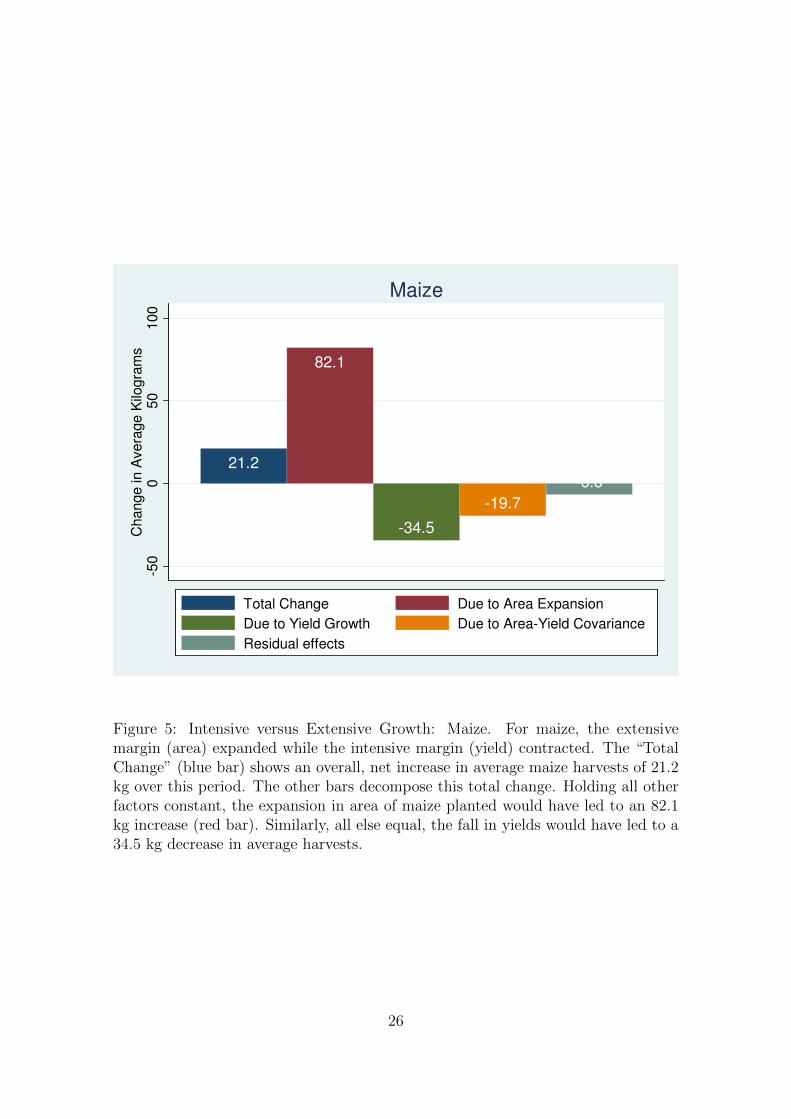
Combining all three of these forces, Figures 5 - 8 implement the decomposition

24

of output growth presented in equation (4). Results are described in the footnote

to each table. Once again, with the exception of rice paddy, small increases in total

output are the net e↵ect of area expansion (positive force) and declining yields and

an increasingly negative farm size–productivity relationship (both driving output

down).

25

21.2

82.1

-34.5

-19.7

-6.8

-50

050

100

Change in

Ave

rage K

ilogra

ms

Maize

Total Change Due to Area Expansion

Due to Yield Growth Due to Area-Yield Covariance

Residual effects

Figure 5: Intensive versus Extensive Growth: Maize. For maize, the extensivemargin (area) expanded while the intensive margin (yield) contracted. The “TotalChange” (blue bar) shows an overall, net increase in average maize harvests of 21.2kg over this period. The other bars decompose this total change. Holding all otherfactors constant, the expansion in area of maize planted would have led to an 82.1kg increase (red bar). Similarly, all else equal, the fall in yields would have led to a34.5 kg decrease in average harvests.

26

22.0

-7.9

47.5

-14.4

-3.2

-20

020

40

60

Change in

Ave

rage K

ilogra

ms

Paddy

Total Change Due to Area Expansion

Due to Yield Growth Due to Area-Yield Covariance

Residual effects

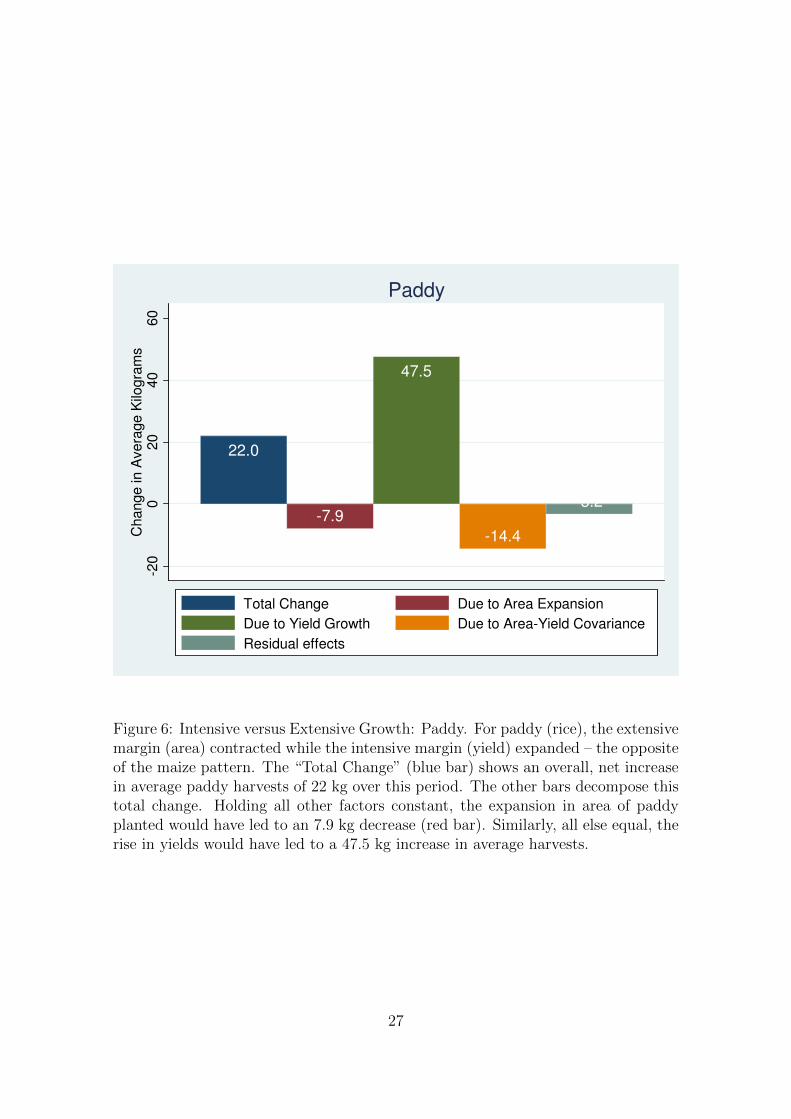
Figure 6: Intensive versus Extensive Growth: Paddy. For paddy (rice), the extensivemargin (area) contracted while the intensive margin (yield) expanded – the oppositeof the maize pattern. The “Total Change” (blue bar) shows an overall, net increasein average paddy harvests of 22 kg over this period. The other bars decompose thistotal change. Holding all other factors constant, the expansion in area of paddyplanted would have led to an 7.9 kg decrease (red bar). Similarly, all else equal, therise in yields would have led to a 47.5 kg increase in average harvests.

27

-0.2

7.0

-1.6

-4.9

-0.8

-50

510

Change in

Ave

rage K

ilogra

ms

Sorghum

Total Change Due to Area Expansion

Due to Yield Growth Due to Area-Yield Covariance

Residual effects

Figure 7: Intensive versus Extensive Growth: Sorghum. For sorghum, the extensivemargin (area) expanded while the intensive margin (yield) contracted. The notablefeature here is the change in the covariance of area and yield over time, i.e., the farmsize-productivity relationship. The “Total Change” (blue bar) shows that overall,there was virtually zero change in average sorghum harvests over this period. Theother bars decompose this total change. Holding all other factors constant, theexpansion in area of sorghum planted would have led to an 7.0 kg decrease (redbar). Similarly, all else equal, the fall in yields would have led to a 1.6 kg decrease inaverage harvests. The change in farm size-productivity relationship reduced harvestsby 4.9 kg, ceteris paribus.

28

-8.1

26.2

-15.5

-8.2-10.6

-20

-10

01

02

03

0C

ha

ng

e in

Ave

rag

e K

ilog

ram

s

Beans

Total Change Due to Area Expansion

Due to Yield Growth Due to Area-Yield Covariance

Residual effects

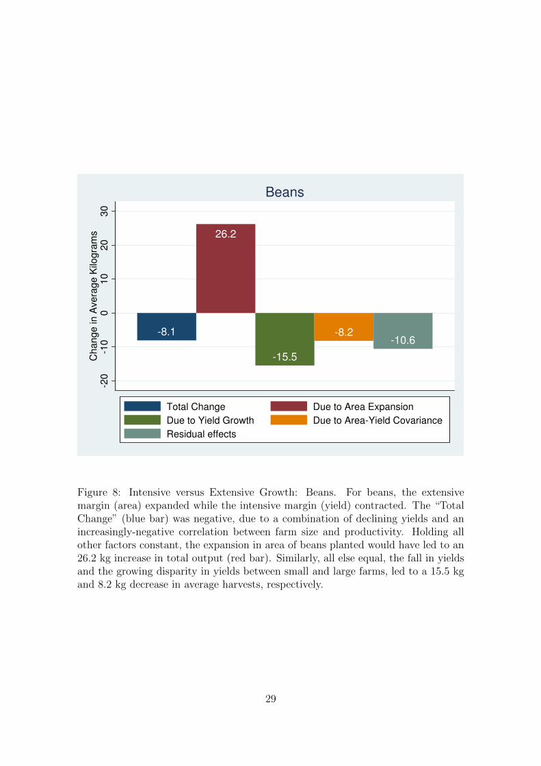
Figure 8: Intensive versus Extensive Growth: Beans. For beans, the extensivemargin (area) expanded while the intensive margin (yield) contracted. The “TotalChange” (blue bar) was negative, due to a combination of declining yields and anincreasingly-negative correlation between farm size and productivity. Holding allother factors constant, the expansion in area of beans planted would have led to an26.2 kg increase in total output (red bar). Similarly, all else equal, the fall in yieldsand the growing disparity in yields between small and large farms, led to a 15.5 kgand 8.2 kg decrease in average harvests, respectively.

29

5 Technology adoption and TFP

The previous section showed that farm yields have been relatively stagnant since

2002/03. In this section we attempt to explain this stagnation by looking at the

determinants of crop yields, and in particular, patterns of technology adoption by

smallholders. Our first task is descriptive: in Section 5.2 we draw on data from

the NSCA and the NPS to measure trends in adoption of new farming techniques

between 2002/03 and 2008/09, and in Section 5.3 we estimate comparable crop-level

production functions for both years to enable measurement of trends in farm-level

total factor productivity over time. Our second, more ambitious task is to explain

why technology adoption has stagnated, which we explore through more detailed

analysis of crop-level production functions in Section 5.4.

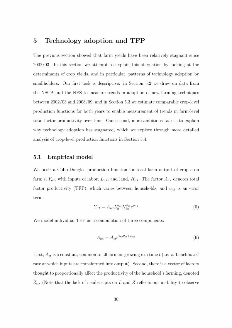
5.1 Empirical model

We posit a Cobb-Douglas production function for total farm output of crop c on

farm i, Yict, with inputs of labor, Lict, and land, Hict. The factor Aict denotes total

factor productivity (TFP), which varies between households, and �ict is an error

term.

Yict = AictL↵ctit H�ct

ict e�ict (5)

We model individual TFP as a combination of three components:

Aict = ActeZit✓ct+µict (6)

First, Act is a constant, common to all farmers growing c in time t (i.e. a ’benchmark’

rate at which inputs are transformed into output). Second, there is a vector of factors

thought to proportionally a↵ect the productivity of the household’s farming, denoted

Zit. (Note that the lack of c subscripts on L and Z reflects our inability to observe

30

these variables disaggregated by crop in the NSCA; data for these variables is at

the household level.) This vector includes indicators of organic or inorganic fertilizer

usage, of using improved seeds for sowing, of irrigating some of the household’s plots,

and of household characteristics. Finally, there is a residual term, µict.

Substituting the expression in (6) for Act in equation (5) gives us the following

production function

Yict = ActL↵ctict H

�ctict e

Zict✓ct+�ict+µict

Dividing both sides by land area, Hict, and denoting divisions by Hict with lower

case letters, we get

yict = Actl↵tictH

↵t+�t�1

ict eZict✓ct+"ict

where the composite error term "ict = �ict + µict. Taking logs of both sides we have

a linear equation, which is the basis for our econometric estimation:

ln(yict) = ln(Act) + ↵ct ln(lict) + �ct ln(Hict) + Zict✓ct + "ict (7)

where �ct = ↵ct + �ct � 1, and H0

: �ct = 0 is a test for constant returns to scale,

with values of � < 0 indicating decreasing returns to scale and � > 0 indicating

increasing returns. The residual term, "ict, will pick up any variation in unobserved

factors important for production, such as unobserved variation in the individual

households’ TFP (in µict), and other factors related to farming such as rainfall (in

�ict).

Endogeneity is a serious concern here. There may be legitimate reasons to sus-

pect that some of the factors picked up by the error term (µict, the unobserved part

of the household’s TFP), such as the innate ability, e�ciency, health, etc., of indi-

vidual farmers may be correlated with the explanatory variables in the regression.

Most importantly, the decision to adopt improved farming methods may be corre-

31

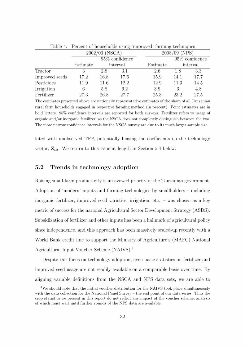
Table 4: Percent of households using ‘improved’ farming techniques2002/03 (NSCA) 2008/09 (NPS)

95% confidence 95% confidenceEstimate interval Estimate interval

Tractor 3 2.8 3.1 2.6 1.8 3.3Improved seeds 17.2 16.8 17.6 15.9 14.1 17.7Pesticides 11.9 11.6 12.2 12.9 11.3 14.5Irrigation 6 5.8 6.2 3.9 3 4.8Fertilizer 27.3 26.8 27.7 25.3 23.2 27.5The estimates presented above are nationally representative estimates of the share of all Tanzanian

rural farm households engaged in respective farming method (in percent). Point estimates are in

bold letters. 95% confidence intervals are reported for both surveys. Fertilizer refers to usage of

organic and/or inorganic fertilizer, as the NSCA does not completely distinguish between the two.

The more narrow confidence intervals for the NSCA survey are due to its much larger sample size.

lated with unobserved TFP, potentially biasing the coe�cients on the technology

vector, Zict. We return to this issue at length in Section 5.4 below.

5.2 Trends in technology adoption

Raising small-farm productivity is an avowed priority of the Tanzanian government.

Adoption of ‘modern’ inputs and farming technologies by smallholders – including

inorganic fertilizer, improved seed varieties, irrigation, etc. – was chosen as a key

metric of success for the national Agricultural Sector Development Strategy (ASDS).

Subsidization of fertilizer and other inputs has been a hallmark of agricultural policy

since independence, and this approach has been massively scaled-up recently with a

World Bank credit line to support the Ministry of Agriculture’s (MAFC) National

Agricultural Input Voucher Scheme (NAIVS).4

Despite this focus on technology adoption, even basic statistics on fertilizer and

improved seed usage are not readily available on a comparable basis over time. By

aligning variable definitions from the NSCA and NPS data sets, we are able to

4We should note that the initial voucher distribution for the NAIVS took place simultaneouslywith the data collection for the National Panel Survey – the end point of our data series. Thus thecrop statistics we present in this report do not reflect any impact of the voucher scheme, analysisof which must wait until further rounds of the NPS data are available.

32

produce comparable statistics on the usage of such ’improved’ farming techniques,

providing a first glimpse of technology adoption patterns over the past several years.

In Table 4 we present estimates of the share of rural Tanzanian farming house-

holds that use improved seeds, fertilizer, pesticides (including fungicides and her-

bicides), irrigation of plots and tractors. The results in Table 4 show very small

changes in adoption of improved farming methods between the two survey years.

The estimates of adoption are generally low, with about one in four farmers using

some kind of fertilizer (organic or inorganic), about one in six use improved seeds,

one in eight use some kind of pesticide/herbicide/fungicide, and only about three

percent reports using a tractor in farming. While the point estimates on tractor

use, improved seeds and fertilizer are somewhat lower in 2008 than in 2002, and

that of pesticides shows a small increase, the di↵erences between the two years are

statistically insignificant. There is, however, a statistically significant decline from

the already rather low level of six percent of households irrigating plots in 2002

to 3.9 percent in 2008. Of course, estimates of irrigation usage may vary between

years depending on di↵ering needs to irrigate plots due to variation in the amount

of rainfall. Still, the low and decreasing figure for irrigation is hardly a good sign,

especially given that a little more than 20 percent of the households reported not

harvesting the entire area they had planted due to droughts in 2008.

Overall, this comparison of farming techniques between 2002/03 and 2008/09

shows consistently low levels of adoption, and lends no support to the hypothesis of

increased productivity in farming due to adoption of more modern farming methods

among small-scale farmers between the survey years.

5.3 Trends in TFP

We measure trends in total factor productivity (TFP) over time by estimating equa-

tion (7) using pooled data from the two survey rounds (i.e., the NSCA and the NPS).

33

We carry out separate estimation for the three most common crops for which we

have comparable data, namely maize, beans and rice paddy. The results of these

estimations are presented in Tables 5-7 below.5 The dependent variable in all these

estimations are yields (i.e. output per acre).

The tables are organized as follows. For each crop, column (1) pools data for

both years and regresses log yields on a constant and a dummy for the 2008 season.

The coe�cient on the 2008 dummy represents approximate percentage change in

yields over this period. Columns (2) and (3) present the full production function

specification from equation (7), estimated separately for each survey round. Column

(4) lists the di↵erence in point coe�cients between the two years and tests for

di↵erences in these returns to factor inputs. The F-test at the bottom of column

(4) is a test for pooling, i.e., whether the data rejects common factor coe�cients

across years. The null hypothesis of equality of parameters is rejected for all crops.

Nevertheless, for the sake of transparency, column (5) presents the results from a

pooled regression where all parameters except the intercepts are restricted to be the

same in both years.

Column (1) replicates the findings from Section 4. As noted in Table 3, yields

have generally been found to be decreasing (with the notable exception of paddy),

whereas area cultivated has increased between the survey years. The new land taken

into use for crop growing is likely less productive than that previously in use (worse

soil quality, steeper slopes of plots, longer distances from home, etc.). To the extent

that previously farmed plots have been expanded, a decrease of the land parameter

5Our ability to empirically measure the variables in equation (7) is much better in the 2008/09NPS than the 2002/03 NSCA. In Tables 5-7 we take the ‘lowest common denominator’ of bothsurveys, limiting ourselves to the somewhat crude indicators measured comparably over time toestimate pooled production functions for 2002/03 and 2008/09. The most detailed variables inthese estimations are measured at the household-crop level (as opposed to the plot-crop levelwhich would have been desirable); fertilizer usage is measured by a dummy indicator rather thanbeing treated as a quantity input; and labor is measured as the number of people in the householdinvolved in agriculture during the past year. In Section 5.4 we are able to estimate more preciseproduction functions using only the NPS 2008/09 data.

34

between columns (2) and (3), indicating more decreasing returns to scale, should

follow. Likewise, to the extent that new, less productive plots have been brought

under cultivation, a decrease in farm e�ciency should follow. Hence the results here

corroborate the trends reported in the previous section. 6

Looking at the tables for maize and beans, the both statistically and economically

significant decreases in yields between the years in column (1) in Tables 5 and 7

can only to a small extent be explained by the inclusion of the other explanatory

variables in column (5). This means that the decline in TFP does not seem to

be due to changes in the input, technology or human capital variables included.

However, as the pooling restrictions for the estimations of column (5) were rejected

for all three crops, columns (2) and (3) of tables 5 to 7 removes those restrictions

and allows the parameters of all variables to vary between the two surveys.

The parameters of the variables on improved farming techniques included - i.e.

the use of fertilizer, improved seeds, pesticides, irrigation and tractors - remain

rather stable between the survey years. Noteworthy deviations from that result are

the estimated coe�cients of pesticide usage in maize production and fertilizer usage

in paddy production. In both cases, one should note that the variables included

are dummy indicators (due to the limits of survey compatibility), so di↵erences

in parameters may be due to changing quantities of pesticides and fertilizer used

among the households that have adopted fertilizer or pesticides. Furthermore, the

coe�cient on the pesticide variable should vary between years, depending on the

existence of pests. With few pests present, the e↵ect of pesticide usage should be

negligible.

Up to this point we have ignored the role of rainfall, which is obviously an

important determinant of farm yields. Apparent di↵erences in TFP as measured in

column (5), for instance, may be due to di↵erences between years in rainfall patterns.

6Unfortunately, as the NSCA data does not include any information at the plot level, we cannotinvestigate to what extent the area expansion is due to larger plots or due to more plots.

35

Columns (6) and (7) address this issue by testing whether our estimates of TFP

changes are a↵ected by controlling for regional rainfall measures from the Tanzanian

Meteorological Agency. Column (6) reproduces the specification in column (5), but

limited to the set of regions for which rainfall is available. Because the rainfall

coverage is somewhat incomplete (note the drop in the observation count), we also

add regional dummies in these last two columns to adjust for any inconsistencies

in the sample coverage over time. Finally, column (7) includes cumulative rainfall

from March to April as a regressor, as well as rainfall squared.

As seen in Tables 5 and 7, the changes in TFP measured in column (5) are

either unchanged or reinforced by controlling for rainfall. TFP fell by 27% for maize,

rose by 22% for rice paddy, and fell by 65% for beans. While not shown here in

the interests of space, replicating these regressions using a more flexible functional

form – i.e., by including the linear and quadratic measure of rainfall in each of

the 12 months of the relevant year, 24 additional regressors in all – also produces

qualitatively similar trends in underlying TFP. These results are also consistent with

the findings of Kirchberger and Mishili (2011) who find that the 46% decline in total

farm output in Kagera from 1991 to 2004 is not explained by changes in input usage,

but instead is larger after controlling for inputs.

To summarize the results from these regressions, while pooling is formally re-

jected, there is broad consistency in the determinants of crop yields from 2002/03 to

2008/09. Apart from the decreasing returns to land size becoming more accentuated,

we find very little evidence of any systematic change in the returns to factor inputs

or farming technologies over time. On the contrary, the secular decline in maize and

bean yields appears almost entirely due to a significant decline in underlying total

factor productivity.

36

5.4 Is fertilizer profitable?

Section 5.2 showed that there has been little or no increase in the use of modern

inputs by smallholders over the past several years in Tanzania. This begs the fun-

damental question of why small farmers fail to adopt modern inputs? There is stark

disagreement in the academic literature on this issue. At risk of oversimplification,

the camps can be grouped into advocates of two broad propositions (acknowledging

that the answer may di↵er across crops, technologies, regions, etc.):

1. Modern technologies are, on average, profitable for smallholders, but farmers

fail to adopt these profitable new inputs because of the uninsured risks asso-

ciated with high-volatility technologies (Dercon and Christiaensen 2010), an

inability to save up for lumpy inputs (Duflo, Kremer, and Robinson 2009), etc.

2. Regardless of the average returns across the population, modern technologies

are simply not profitable for smallholders given their scale, soil type, market

access and/or ability to a↵ord other complementary inputs (Suri 2011, Zeitlin,

Teal, Caria, Dzene, and Opoku 2010).

In either case, input subsidies such as the NAIVS, discussed above, may succeed in

raising technology adoption rates. The question is whether this is desirable. If the

first proposition is true in the case of fertilizer and improved maize seeds in Tanzania,

then the NAIVS will be socially welfare improving by helping to overcome market

failures and raising national output.7 If, on the other hand, the second proposition

is true, NAIVS will be a net loss. Though such subsidies may still be justified as

a form of welfare redistribution, they will detract from overall economic e�ciency

and, in all likelihood, growth.

7Of course, even if the policy is welfare improving it may not be ‘desirable’ in competition withother policies if the government has limited resources. Such an evaluation of desirability naturallyfalls outside the scope of this study.

37

This section asks whether – and for whom – adopting modern technologies is

profitable. We build on the production function specification from Section 5.3, but

restrict ourselves to the 2008/09 NPS data. Doing so allows us to exploit the finer

detail of this newer data, measuring fertilizer and pesticides as continuous variables

alongside land and labor. Hence, we revise the specification in (5) and adopt the

following production function :

Yic = AcL↵icF

�11,icF

�22,icF

�33,icH

�ice

Zic✓c+�ic+µic , (8)

where F1

, F2

and F3

are quantities of inorganic and organic fertilizer and pesticides

respectively. In the cases of inorganic fertilizer and pesticides, these are not ho-

mogenous inputs, and hence we measure these by their costs (in thousands of TSH)

rather than physical quantities.

Dividing by land area and taking logs, we get the equivalent of equation (7):

ln(yic) = ln(Ac)+↵ ln(lic)+�1

ln(f1,ic)+�

2

ln(f2,ic)+�

3

ln(f3,ic)+�Hic+Zic✓c+ "ic.

(9)

OLS estimates of equation (9) for maize, beans and paddy are presented in

Table 9. While the coe�cients of the estimations here are not strictly comparable

to those in Tables 5-7 above, the results remain qualitatively similar. There are

decreasing returns to scale, as the parameter of on land is negative and statistically

significant for all crops; the usage use of inorganic and organic fertilizer, pesticides

and tractors are each significantly correlated with higher yields, except in the case

of beans where small samples undermine statistical significance for some inputs.

Somewhat surprisingly, the parameter on improved seed usage are is statistically

insignificant in all estimates and even negative for both maize and paddy.

38

Interpreting these estimates further is di�cult without taking careful account of

possible endogeneity concerns. Some of these concerns are beyond the limits of our

data set to address. However, the empirical model in equations (8) and (9) provides

a framework to structure our discussion of existing empirical research on the returns

to fertilizer, which we organize around three types of heterogeneity that may a↵ect

our results:

1. Unobserved fixed e↵ects, µic

2. Heterogeneity in the returns to inputs, e.g., variation over i in ✓ic

3. Price variation a↵ecting the profitability of fertilizer at a given marginal prod-

uct.

The following sections discuss these three issues, placing the results of our relatively

simple, cross-section, OLS production function estimates for Tanzania in the context

of earlier experimental and longitudinal research for other countries.

5.4.1 Are adopters & non-adopters comparable?

Our estimation of the return to fertilizer derives from a comparison of yields be-

tween ‘adopters’ (i.e., fertilizer users) and non-adopters, controlling for observed

factor inputs. These groups may be non-comparable in ways unobserved to the

econometrician. As already noted, OLS estimates of ✓ will be biased upward if

farmers’ idiosyncratic TFP, µict, is positively correlated with fertilizer usage.

In order to estimate the financial return to fertilizer and overcome this source of

bias, Duflo et al. (2009) exploit a randomized field experiments of fertilizer applica-

tion in maize production. Randomization ensures complete comparability between

adopters and non-adopters. Relative to many similar agronomic experiments, this

particular trial is attractive in that it takes place on real-world, small-scale farms.

39

In this highly controlled setup, Duflo et al. find that application of inorganic

fertilizer produces significant physical returns and that these are – with a specific set

of prices, discussed more below – highly profitable. The optimal level of fertilization

has a mean financial return of about 36 percent over one season. They explore non-

linearities in the return, and find that applying the o�cially recommended amount

of improved seeds and fertilizer (twice the amount of the most profitable level in

the study) is highly unprofitable. Likewise, applying too little fertilizer (half the

optimal level) is highly unprofitable for most farmers.

Nevertheless, the main result to take away from the Duflo, et al. experiment is

that high physical returns to fertilizer on actual smallholder farmers in East Africa

are not entirely due to selection or unobserved TFP.

5.4.2 Can new adopters expect the same returns?

Even if adopters and non-adopters have comparable TFP levels, both OLS and IV

estimates will only capture the return to fertilizer for farmers who are observed

using fertilizer – i.e., a “local average treatment e↵ect” or the “average treatment

for the treated” to adopt the treatment e↵ects terminology. If such heterogeneity is

(positively) correlated with adoption, then finding that fertilizer is profitable does

not

Suri (2011) studies the heterogeneity of returns to adopting modern farm tech-

nologies in the form of using improved seeds. She allows for heterogeneity in both

the costs and benefits to technology adoption across farmers (i.e. di↵ering returns).

Using panel data from Kenya, she finds that the persistent lack of adoption can be

explained by these di↵erences; farmers are rational and complete adoption is unde-

sirable. There is more than one side to this story though. Some farmers with very

high returns to technology are supply constrained, i.e. their costs for adoption is

high due to underdeveloped supply. Developing the supply side of such technologies

40

would yield adoption profitable for these farmers.

Turning to our estimates from Tanzania, we lack the data to allow for the scope

of heterogeneity modeled in Suri’s Kenyan data. However, the basic Cobb-Douglas

specification we employ implicitly allows for limited heterogeneity in the return to

fertilizer across farmers. To see this, note that assuming the production function

specification in equation (9) the marginal e↵ect of using inorganic fertilizer in equa-

tion is given by:@Yic

@F1,ic

= �1

yicf1,ic

(10)

This marginal e↵ect depends on the parameter on inorganic fertilizer, �1

, as well

as the level of yield on the plot, yic, and the intensity of fertilizer usage, fic. As

the marginal e↵ect varies with yield, we evaluate the ‘e↵ect’ of fertilizer use at the

median of yict for all households, for fertilizing households, and for non-fertilizing

households separately. As the e↵ect also varies with the intensity of fertilization,

we evaluate the discrete increase of fertilization from zero to the mean of intensity

among the households using fertilization. The results of these calculations can be

seen in Table 10 below.

Table 10 shows that the median yield among households using inorganic fertilizer

is substantially higher than among non-fertilizer for maize and rice paddy.8 The ob-

served di↵erences in average yields between the households may come about because

of the di↵erence in fertilization itself, di↵erences in other inputs, or di↵erent TFP’s.

As we cannot completely disentangle these factors, we present yields ’as is’ here. In

the calculations of profitability we will rely on the median yield of all households as

this is the most robust measure.8Deducting the estimated ‘e↵ect’ of fertilization, the adjusted yield for the median household

among those using fertilizer is much closer to that of the non-users. For maize, the whole di↵erencein yields virtually disappears, indicating that the doubling of median yield among users seems tostem from fertilization. However, for beans we see the opposite pattern, with fertilizing householdshaving lower yields than others – a picture that is reinforced when adjusting for the e↵ect offertilization.

41

Table 10 also shows estimates of returns to fertilizer based on the Cobb-Douglas

production function given in in equation (9). Looking at the return to inorganic

fertilizer, an investment of 1,000 TSH in inorganic fertilizer will increase production

by almost 7 kg’s for maize, between 5.2 and 6.5 kg’s for paddy and between 1.25

and 2 kg’s for beans base. Hence, looking at the median yield of all non-fertilizing

households, the price of output required for an inorganic fertilizer investment to

bear its cost is about 150 TSH per kg of maize, just below 200 TSH per kg of paddy,

and just over 500 TSH per kg of beans.

5.4.3 Which crop price is relevant for profitability?

Crop prices vary considerably over the growing season and across regions at a given

point in time. Within a given region, the farm-gate price available to a remote

producer may be far below the sale price in urban market centers. The profitability

of fertilizer will hinge to a large degree on which price is used.

Lack of relevant price data is a major shortcoming of much existing research on

this topic. Table 8 lists the existing measures of the return to fertilizer that we

were able to locate for Tanzania. The value to cost ratio, defined as the increase

in gross income from application of inorganic fertilizer divided by the marginal cost

of the input, is the measure comparable to those of Duflo et al. (2009) and Suri

(2011) discussed above. The returns vary between 100 to 1400 percent depending on

location of study. Moreover, these estimates of price incentives relies on price data

from published FAO data, and hence provide a quite crude guide to the potential

viability of a fertilizer program.

Similar concerns arise with respect to the experimental evidence from Duflo et

al. (2009) discussed above. The authors’ calculations of a profitable return to

fertilizer use assume farmers sell (and/or forego purchase of) maize just before the

next cropping season, when the maize price is at its highest. If sales occurred at

42

any other time, the returns would decrease substantially, as market prices for maize

vary considerably over the year.

The NPS data allows us to compare various relevant prices for smallholder farm-

ers in Tanzania. These are presented in Table 11. The median sales price for maize

is just over 200 TSH, about 400 TSH for paddy and 500 TSH for beans. The sales

prices are somewhat higher among the fertilizing households, especially in the case

of beans. As many of the households are net buyers of crop, one can make a case for

valuing the output at purchasing prices instead, as an increased harvest may make

less purchases needed. Hence, we also present the median price paid for maize,

paddy and beans by the maize, paddy and beans growing households respectively.

It is evident from Table 11 that with the exception of paddy, quite a few of the

households have bought some quantity of a crop (consumed in the week just be-

fore the interview ) that they are growing themselves. The median prices paid are,

unsurprisingly, higher than the sales prices.

In view of this evidence, given that the di↵erent prices reported by the households

are often higher than the price required to break even, it seems that investment in

inorganic fertilizer has the potential of being profitable for farmers. In order to see

exactly how profitable, and to be able to compare these results to those of previous

researchers, we calculate the return to inorganic fertilizer as the value to cost ratio.

That is, using the six di↵erent output prices in Table 11, we value the estimated

increase in output due to fertilization, and divide this by the cost of fertilization.

The results are presented in Table 12.

Based on our estimations of the return to inorganic fertilizer, and the three

di↵erent categories of sales prices reported in the NPS, it seems from Table 12

that inorganic fertilizer usage is in a strict economic sense on average economically

profitable for farmers. The only exception to this rule is when including the non-

fertilizing households in the selling price of beans, which makes the investment

43

in fertilizer just pay back its cost. If one considers the purchasing prices, which

are higher than sales prices, the returns grow even larger. However, a common

rule of thumb is that an estimated value-to-cost ratio of about 2 is needed for

small-holder farmers to start using fertilizer, as fertilization not only brings higher

average revenues but also a high variation in revenues. This is true both between

farmers and between seasons: between farmers as the estimated adoption rates

may, as mentioned, reflect the benefits only among those who can be expected to

benefit the most; between seasons as the fertilizers do not give the same e↵ect each

season, potentially even making adoption non-profitable in some years. Hence, while

fertilization may be profitable on average for the individual farmer, there may still

be rational grounds for why fertilization has not been picked up by more households.

Returning to the value-to-cost ratios, which of the prices in Table 12 makes

most sense to use will vary from household to household. For instance, the fact that

fertilizing households have both higher sales and higher consumption prices indicate

that they are situated in areas where crop prices are higher. This highlight the fact

that location is an important aspect to consider. Moreover, whether a household

is a net buyer or net seller of crops will be highly important for the valuation of

the harvest. From the high variability in returns to fertilizer presented in Table 12,

it is evident that taking all these factors into consideration is key when assessing

profitability.

44

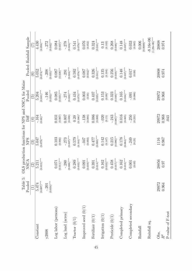
Tab

le5:

OLSproductionfunctionsforNPSan

dNSCA

forMaize

Poo

led

NSCA

NPS

Di↵

Poo

led

Poo

led–R

ainfallSam

ple

(1)

(2)

(3)

(4)

(5)

(6)

(7)

Con

stan

t5.474

5.211

5.047

-.164

5.204

5.052

4.430

(0.007)

⇤⇤⇤

(0.015)

⇤⇤⇤

(0.079)

⇤⇤⇤

(0.08)

⇤⇤(0.041)

⇤⇤⇤

(0.074)

⇤⇤⇤

(0.094)

⇤⇤⇤

y2008

-.201

-.146

-.208

-.272

(0.034)

⇤⇤⇤

(0.032)

⇤⇤⇤

(0.035)

⇤⇤⇤

(0.042)

⇤⇤⇤

Log

labor

(persons)

0.071

0.103

0.031

0.085

0.087

0.084

(0.011)

⇤⇤⇤

(0.066)

(0.067)

(0.031)

⇤⇤⇤

(0.038)

⇤⇤(0.037)

⇤⇤

Log

land(acres)

-.280

-.273

0.007

-.274

-.291

-.278

(0.008)

⇤⇤⇤

(0.037)

⇤⇤⇤

(0.038)

(0.022)

⇤⇤⇤

(0.024)

⇤⇤⇤

(0.024)

⇤⇤⇤

Tractor

(0/1)

0.289

0.579

0.29

0.434

0.592

0.541

(0.032)

⇤⇤⇤

(0.164)

⇤⇤⇤

(0.166)

⇤(0.073)

⇤⇤⇤

(0.078)

⇤⇤⇤

(0.079)

⇤⇤⇤

Improvedseed

(0/1)

0.091

-.047

-.138

0.003

0.087

0.076

(0.019)

⇤⇤⇤

(0.093)

(0.094)

(0.05)

(0.052)

⇤(0.052)

Fertilizer(0/1)

0.391

0.477

0.086

0.437

0.326

0.324

(0.014)

⇤⇤⇤

(0.068)

⇤⇤⇤

(0.069)

(0.035)

⇤⇤⇤

(0.041)

⇤⇤⇤

(0.041)

⇤⇤⇤

Irrigation

(0/1)

0.162

0.142

-.020

0.153

0.135

0.13

(0.033)

⇤⇤⇤

(0.147)

(0.15)

(0.09)

⇤(0.104)

(0.103)

Pesticide(0/1)

0.458

0.215

-.243

0.323

0.256

0.268

(0.017)

⇤⇤⇤

(0.086)

⇤⇤(0.087)

⇤⇤⇤

(0.049)

⇤⇤⇤

(0.049)

⇤⇤⇤

(0.049)

⇤⇤⇤

Com

pletedprimary

0.162

0.178

0.016

0.165

0.148

0.148

(0.013)

⇤⇤⇤

(0.064)

⇤⇤⇤

(0.065)

(0.034)

⇤⇤⇤

(0.037)

⇤⇤⇤

(0.037)

⇤⇤⇤

Com

pletedsecondary

0.001

-.249

-.250

-.091

0.017

0.033

(0.03)

(0.23)

(0.231)

(0.086)

(0.09)

(0.085)

Rainfall

0.006

(0.0009)

⇤⇤⇤

Rainfallsq.

-8.16e-06

(1.29e-06)

⇤⇤⇤

Obs.

29972

28856

1116

29972

29972

20808

20808

R2

0.964

0.97

0.967

0.968

0.968

0.974

0.974

P-valueof

F-test

.043

45

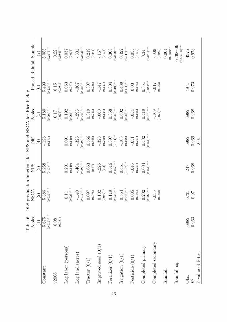
Tab

le6:

OLSproductionfunctionsforNPSan

dNSCA

forRicePad

dy

Poo

led

NSCA

NPS

Di↵

Poo

led

Poo

led–R

ainfallSam

ple

(1)

(2)

(3)

(4)

(5)

(6)

(7)

Con

stan

t5.675

5.386

5.258

-.128

5.180

5.493

5.055

(0.013)

⇤⇤⇤

(0.036)

⇤⇤⇤

(0.17)

⇤⇤⇤

(0.171)

(0.094)

⇤⇤⇤

(0.235)

⇤⇤⇤

(0.277)

⇤⇤⇤

y2008

0.08

0.17

0.15

0.22

(0.081)

(0.076)

⇤⇤(0.081)

⇤(0.084)

⇤⇤⇤

Log

labor

(persons)

0.11

0.201

0.091

0.192

0.053

0.037

(0.023)

⇤⇤⇤

(0.149)

(0.149)

(0.065)

⇤⇤⇤

(0.077)

(0.076)

Log

land(acres)

-.140

-.464

-.325

-.295

-.307

-.301

(0.017)

⇤⇤⇤

(0.096)

⇤⇤⇤

(0.095)

⇤⇤⇤

(0.046)

⇤⇤⇤

(0.053)

⇤⇤⇤

(0.053)

⇤⇤⇤

Tractor

(0/1)

0.097

0.663

0.566

0.319

0.307

0.219

(0.078)

(0.57)

(0.565)

(0.243)

(0.236)

(0.244)

Improvedseed

(0/1)

0.102

-.226

-.328

-.060

-.147

-.167

(0.049)

⇤⇤(0.3)

(0.299)

(0.124)

(0.121)

(0.113)

Fertilizer(0/1)

0.119

0.516

0.397

0.358

0.304

0.308

(0.036)

⇤⇤⇤

(0.152)

⇤⇤⇤

(0.154)

⇤⇤(0.089)

⇤⇤⇤

(0.091)

⇤⇤⇤

(0.092)

⇤⇤⇤

Irrigation

(0/1)

0.564

0.461

-.103

0.602

0.439

0.422

(0.043)

⇤⇤⇤

(0.197)

⇤⇤(0.198)

(0.083)

⇤⇤⇤

(0.111)

⇤⇤⇤

(0.117)

⇤⇤⇤

Pesticide(0/1)

0.005

-.046

-.051

-.054

0.03

0.055

(0.085)

(0.251)

(0.261)

(0.195)

(0.175)

(0.179)

Com

pletedprimary

0.202

0.634

0.432

0.419

0.351

0.34

(0.027)

⇤⇤⇤

(0.151)

⇤⇤⇤

(0.151)

⇤⇤⇤

(0.076)

⇤⇤⇤

(0.08)

⇤⇤⇤

(0.081)

⇤⇤⇤

Com

pletedsecondary

-.055

-.169

-.017

-.009

(0.062)

(0.075)

⇤⇤(0.083)

(0.082)

Rainfall

0.004

(0.002)

⇤⇤

Rainfallsq.

-7.30e-06

(2.55e-06)

⇤⇤⇤

Obs.

6982

6735

247

6982

6982

4975

4975

R2

0.963

0.97

0.968

0.969

0.968

0.973

0.973

P-valueof

F-test

.001

46

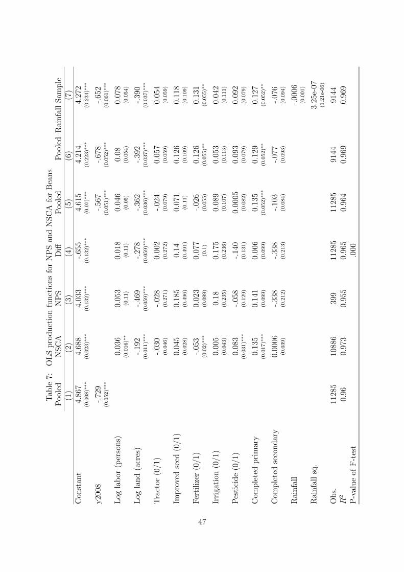
Tab

le7:

OLSproductionfunctionsforNPSan

dNSCA

forBeans

Poo

led

NSCA

NPS

Di↵

Poo

led

Poo

led–R

ainfallSam

ple

(1)

(2)

(3)

(4)

(5)

(6)

(7)

Con

stan

t4.867

4.688

4.033

-.655

4.615

4.214

4.272

(0.008)

⇤⇤⇤

(0.023)

⇤⇤⇤

(0.132)

⇤⇤⇤

(0.132)

⇤⇤⇤

(0.07)

⇤⇤⇤

(0.223)

⇤⇤⇤

(0.234)

⇤⇤⇤

y2008

-.729

-.567

-.678

-.652

(0.052)

⇤⇤⇤

(0.051)

⇤⇤⇤

(0.052)

⇤⇤⇤

(0.061)

⇤⇤⇤

Log

labor

(persons)

0.036

0.053

0.018

0.046

0.08

0.078

(0.016)

⇤⇤(0.11)

(0.11)

(0.05)

(0.054)

(0.054)

Log

land(acres)

-.192

-.469

-.278

-.362

-.392

-.390

(0.011)

⇤⇤⇤

(0.059)

⇤⇤⇤

(0.059)

⇤⇤⇤

(0.036)

⇤⇤⇤

(0.037)

⇤⇤⇤

(0.037)

⇤⇤⇤

Tractor

(0/1)

-.030

-.028

0.002

-.024

0.057

0.054

(0.046)

(0.271)

(0.272)

(0.079)

(0.059)

(0.059)

Improvedseed

(0/1)

0.045

0.185

0.14

0.071

0.126

0.118

(0.028)

(0.496)

(0.491)

(0.11)

(0.109)

(0.109)

Fertilizer(0/1)

-.053

0.023

0.077

-.026

0.126

0.131

(0.02)

⇤⇤⇤

(0.099)

(0.1)

(0.055)

(0.055)

⇤⇤(0.055)

⇤⇤

Irrigation

(0/1)

0.005

0.18

0.175

0.089

0.053

0.042

(0.043)

(0.235)

(0.236)

(0.107)

(0.113)

(0.111)

Pesticide(0/1)

0.083

-.058

-.140

0.0005

0.093

0.092

(0.031)

⇤⇤⇤

(0.129)

(0.131)

(0.082)

(0.079)

(0.079)

Com

pletedprimary

0.135

0.141

0.006

0.135

0.129

0.127

(0.017)

⇤⇤⇤

(0.099)

(0.099)

(0.052)

⇤⇤⇤

(0.052)

⇤⇤(0.052)

⇤⇤

Com

pletedsecondary

0.0006

-.338

-.338

-.103

-.077

-.076

(0.039)

(0.212)

(0.213)

(0.084)

(0.093)

(0.094)

Rainfall

-.0006

(0.001)

Rainfallsq.

3.25e-07

(1.21e-06)

Obs.

11285

10886

399

11285

11285

9144

9144

R2

0.96

0.973

0.955

0.965

0.964

0.969

0.969

P-valueof

F-test

.000

47

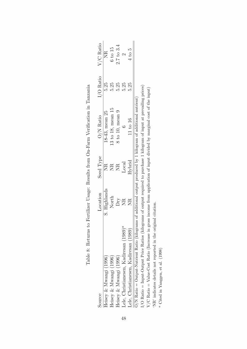
Tab

le8:

Returnsto

FertilizerUsage:Resultsfrom

On-Farm

Verification

inTan

zania

Sou

rce

Location

SeedTyp

eO/N

Ratio

I/O

Ratio

V/C

Ratio

Heisey&

Mwan

gi(1996)

S.Highlands

NR

18-43,

mean25

5.25

NR

Heisey&

Mwan

gi(1996)

North

NR

13to

18,mean15

5.25

6to

15Heisey&

Mwan

gi(1996)

Dry

NR

8to

10,mean9

5.25

2.7to

3.4

Lele,

Christianesen,Kad

iresan

(1989)

aNR

Local

65.25

2Lele,

Christianesen,Kad

iresan

(1989)

NR

Hyb

rid

11to

165.25

4to

5O/N

Ratio

=Output-Nutrient

Ratio

(kilog

ramsof

additional

outputproducedby

1kilogram

ofad

ditional

nutrient)

I/O

Ratio

=Input-OutputPrice

Ratios(kilog

ramsof

outputrequ

ired

topurchase1kilogram

ofinputat

prevailingprices)

V/C

Ratio

=Value-CostRatio

(Increase

ingrossincomefrom

application

ofinputdivided

bymarginal

cost

oftheinput)

‘NR’indicates

details

not

reportedin

theoriginal

citation

.aCited

inYan

ggen,et

al.(199

8)

48

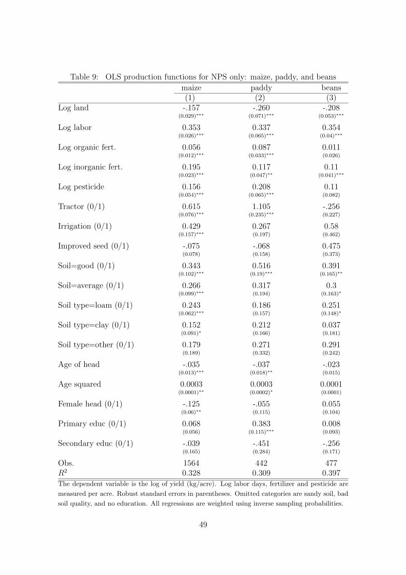
Table 9: OLS production functions for NPS only: maize, paddy, and beansmaize paddy beans(1) (2) (3)

Log land -.157 -.260 -.208(0.029)

⇤⇤⇤(0.071)

⇤⇤⇤(0.053)

⇤⇤⇤

Log labor 0.353 0.337 0.354(0.026)

⇤⇤⇤(0.065)

⇤⇤⇤(0.04)

⇤⇤⇤

Log organic fert. 0.056 0.087 0.011(0.012)

⇤⇤⇤(0.033)

⇤⇤⇤(0.026)

Log inorganic fert. 0.195 0.117 0.11(0.023)

⇤⇤⇤(0.047)

⇤⇤(0.041)

⇤⇤⇤

Log pesticide 0.156 0.208 0.11(0.054)

⇤⇤⇤(0.065)

⇤⇤⇤(0.082)

Tractor (0/1) 0.615 1.105 -.256(0.076)

⇤⇤⇤(0.235)

⇤⇤⇤(0.227)

Irrigation (0/1) 0.429 0.267 0.58(0.157)

⇤⇤⇤(0.197) (0.462)

Improved seed (0/1) -.075 -.068 0.475(0.078) (0.158) (0.373)

Soil=good (0/1) 0.343 0.516 0.391(0.102)

⇤⇤⇤(0.19)

⇤⇤⇤(0.165)

⇤⇤

Soil=average (0/1) 0.266 0.317 0.3(0.099)

⇤⇤⇤(0.194) (0.163)

⇤

Soil type=loam (0/1) 0.243 0.186 0.251(0.062)

⇤⇤⇤(0.157) (0.148)

⇤

Soil type=clay (0/1) 0.152 0.212 0.037(0.091)

⇤(0.166) (0.181)

Soil type=other (0/1) 0.179 0.271 0.291(0.189) (0.332) (0.242)

Age of head -.035 -.037 -.023(0.013)

⇤⇤⇤(0.018)

⇤⇤(0.015)

Age squared 0.0003 0.0003 0.0001(0.0001)

⇤⇤(0.0002)

⇤(0.0001)

Female head (0/1) -.125 -.055 0.055(0.06)

⇤⇤(0.115) (0.104)

Primary educ (0/1) 0.068 0.383 0.008(0.056) (0.115)

⇤⇤⇤(0.093)

Secondary educ (0/1) -.039 -.451 -.256(0.165) (0.284) (0.171)

Obs. 1564 442 477R2 0.328 0.309 0.397The dependent variable is the log of yield (kg/acre). Log labor days, fertilizer and pesticide are

measured per acre. Robust standard errors in parentheses. Omitted categories are sandy soil, bad

soil quality, and no education. All regressions are weighted using inverse sampling probabilities.

49

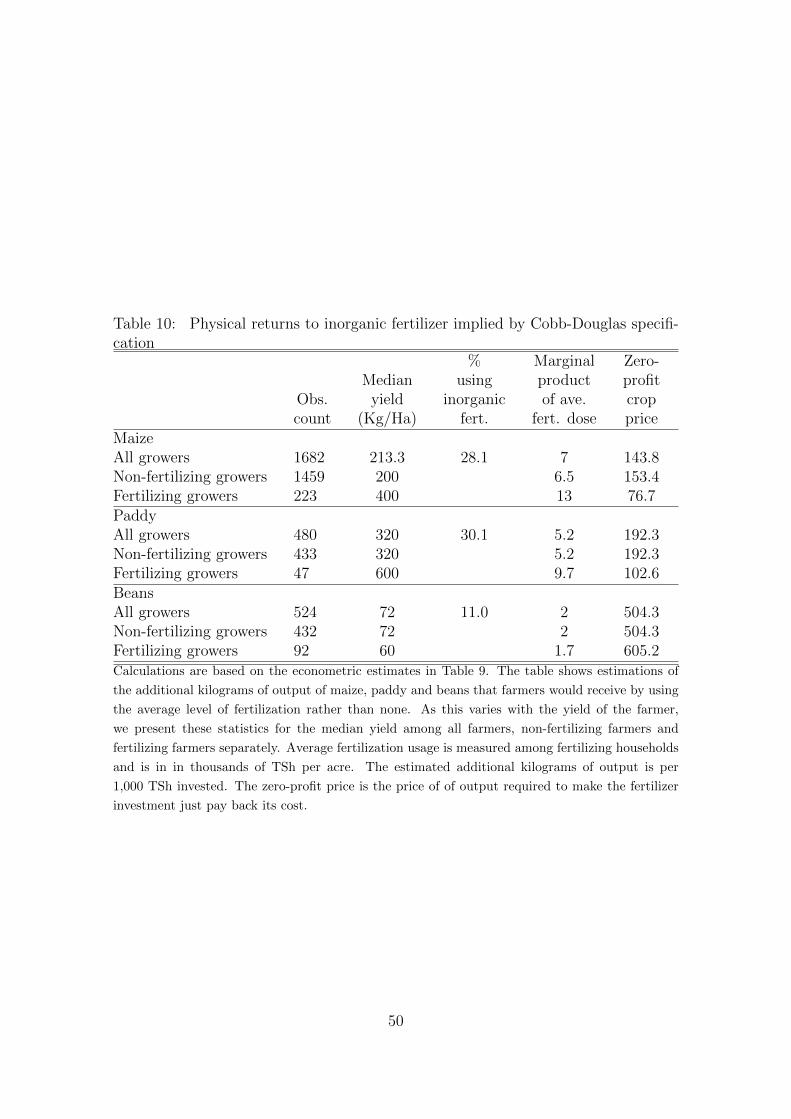
Table 10: Physical returns to inorganic fertilizer implied by Cobb-Douglas specifi-cation

% Marginal Zero-Median using product profit

Obs. yield inorganic of ave. cropcount (Kg/Ha) fert. fert. dose price

MaizeAll growers 1682 213.3 28.1 7 143.8Non-fertilizing growers 1459 200 6.5 153.4Fertilizing growers 223 400 13 76.7PaddyAll growers 480 320 30.1 5.2 192.3Non-fertilizing growers 433 320 5.2 192.3Fertilizing growers 47 600 9.7 102.6BeansAll growers 524 72 11.0 2 504.3Non-fertilizing growers 432 72 2 504.3Fertilizing growers 92 60 1.7 605.2Calculations are based on the econometric estimates in Table 9. The table shows estimations of

the additional kilograms of output of maize, paddy and beans that farmers would receive by using

the average level of fertilization rather than none. As this varies with the yield of the farmer,

we present these statistics for the median yield among all farmers, non-fertilizing farmers and

fertilizing farmers separately. Average fertilization usage is measured among fertilizing households

and is in in thousands of TSh per acre. The estimated additional kilograms of output is per

1,000 TSh invested. The zero-profit price is the price of of output required to make the fertilizer

investment just pay back its cost.

50

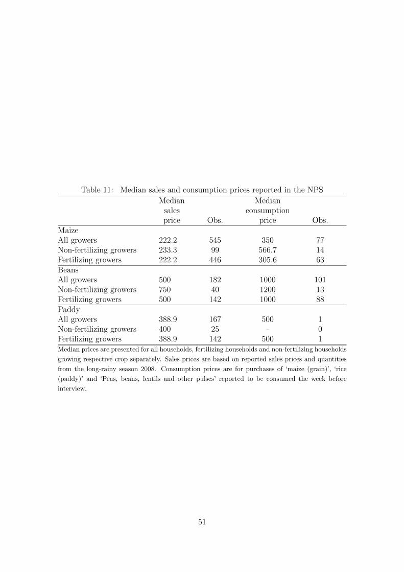
Table 11: Median sales and consumption prices reported in the NPSMedian Mediansales consumptionprice Obs. price Obs.

MaizeAll growers 222.2 545 350 77Non-fertilizing growers 233.3 99 566.7 14Fertilizing growers 222.2 446 305.6 63BeansAll growers 500 182 1000 101Non-fertilizing growers 750 40 1200 13Fertilizing growers 500 142 1000 88PaddyAll growers 388.9 167 500 1Non-fertilizing growers 400 25 - 0Fertilizing growers 388.9 142 500 1Median prices are presented for all households, fertilizing households and non-fertilizing households

growing respective crop separately. Sales prices are based on reported sales prices and quantities

from the long-rainy season 2008. Consumption prices are for purchases of ‘maize (grain)’, ‘rice

(paddy)’ and ‘Peas, beans, lentils and other pulses’ reported to be consumed the week before

interview.

51

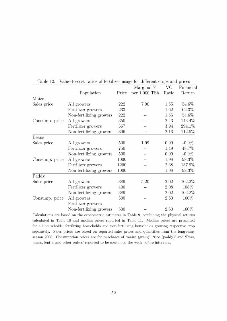
Table 12: Value-to-cost ratios of fertilizer usage for di↵erent crops and pricesMarginal Y VC Financial

Population Price per 1,000 TSh Ratio ReturnMaizeSales price All growers 222 7.00 1.55 54.6%

Fertilizer growers 233 -- 1.62 62.3%Non-fertilizing growers 222 -- 1.55 54.6%

Consump. price All growers 350 -- 2.43 143.4%Fertilizer growers 567 -- 3.94 294.1%Non-fertilizing growers 306 -- 2.13 112.5%

BeansSales price All growers 500 1.99 0.99 -0.9%

Fertilizer growers 750 -- 1.49 48.7%Non-fertilizing growers 500 -- 0.99 -0.9%

Consump. price All growers 1000 -- 1.98 98.3%Fertilizer growers 1200 -- 2.38 137.9%Non-fertilizing growers 1000 -- 1.98 98.3%

PaddySales price All growers 389 5.20 2.02 102.2%

Fertilizer growers 400 -- 2.08 108%Non-fertilizing growers 389 -- 2.02 102.2%

Consump. price All growers 500 -- 2.60 160%Fertilizer growers - -- - -Non-fertilizing growers 500 -- 2.60 160%

Calculations are based on the econometric estimates in Table 9, combining the physical returns

calculated in Table 10 and median prices reported in Table 11. Median prices are presented

for all households, fertilizing households and non-fertilizing households growing respective crop

separately. Sales prices are based on reported sales prices and quantities from the long-rainy

season 2008. Consumption prices are for purchases of ‘maize (grain)’, ‘rice (paddy)’ and ‘Peas,

beans, lentils and other pulses’ reported to be consumed the week before interview.

52

6 Conclusions

To summarize our findings, we return to the three empirical questions posed in

Section 1.

Question 1. Did smallholder productivity growth lift farm households out of poverty?

Or did farmers exit to better opportunities?

In Section 3 we used data from three rounds of the Household Budget Surveys to

show that it has been the decline of the agricultural sector (in terms of employment

shares) rather than growth within the sector (in per capita consumption terms) that

has had the greatest impact on overall consumption levels in Tanzania over the past

two decades. While the overall rate of average consumption growth has been slow,

at approximately 1.1% per annum from 1991 to 2007, over 40% of this growth was

attributable to structural change, i.e., movement out of agriculture and primarily

into non-farm self-employment.

As noted in the introduction, the fact that most poor people in Tanzania earn

their living through small-scale farming does not imply that raising smallholder pro-

ductivity is a policy priority for poverty reduction – though other facts may indeed

justify such a focus (Jayne, Mason, Myers, Ferris, Mather, Beaver, Lenski, Chapoto,

and Boughton 2010). Income diversification and rural to urban migration might be

equally valid strategies, as our findings regarding structural change reinforce. Con-

versely though, international experience showing a close connection between poverty

reduction and a declining share of agriculture in GDP does not provide justifica-

tion for focusing policy on industrial sectors. A variety of theoretical and empiri-

cal evidence suggests that agricultural productivity growth may be a pre-condition

for structural transformation and industrial development (Dercon 2009, Datt and

Ravallion 2002). We emphasize that our descriptive findings alone cannot provide

an answer to this sequencing debate.

53

Question 2. How much has output of major crops increased over this period? Was

the growth of, say, maize output due to (a) productivity increases, or (b) an expan-

sion of the area planted?

Very little comparable data on crop yields over time exists for Tanzania. Aligning

the NSCA 2002/03 and NPS 2008/09 sources of yield information was one of the ma-

jor objectives of this paper. For maize and most other major crops (rice paddy being

the key exception), we find that average yields have actually declined, and where

output growth is present it is primarily attributable to area expansion. While our

analysis was conducted on individual crops, area expansion is found across almost all

major crops, suggesting an expansion in total area planted rather than substitution

between crop varieties. Finally, we also find that an increasingly inverse relationship

between farm size and productivity explains part of the decline in output for staple

crops such as maize and sorghum. This trend is consistent with exacerbated input

market failures in rural areas, though this hypothesis requires further investigation

and more direct corroboration to complement our fairly indirect evidence on this

front.

Question 3. Has use of inorganic fertilizer, hybrid seeds, irrigation, etc. increased?

Why or why not? Are these technologies profitable for smallholders at prevailing

prices?

Beginning with secular trends, we find no increase in use of key modern tech-

nologies such as inorganic fertilizer, hybrid seeds, irrigation, etc. Adoption of these

technologies is low and stable over time. Estimating pooled production functions

across the two rounds of data, we find fairly stable returns to these technologies.

This implies that the declining yields measured in the previous section are primarily

attributable to falling total factor productivity (TFP). This can possibly be ex-

plained by the area expansion, if the new land cultivated is less suited for farming

54

than that previously used. Given the importance of this issue further investigation

to explain the decline of the TFP is needed.

The final question posed in the paper was whether modern inputs, and in partic-

ular inorganic fertilizer, is potentially profitable for smallholder farmers? Estimates

of the rate of return to inorganic fertilizer from the NPS 2008/09 data suggest

that it is. However, our simple estimates of this return are subject to a number of

econometric concerns. Viewing our results in light of existing research from other

countries that has addressed many of these methodological concerns, there is some

cause for optimism that our simple estimates may accurately reflect the true aver-

age return. However, this average return may not be attainable by all farmers due

to heterogeneity in returns and variation in prices. More precise measurement of

this heterogeneity is needed before making a general assessment of the viability of

schemes to promote new technology adoption.

References

Binswanger, H. P., K. Deininger, and G. Feder (1995): “Power, distor-

tions, revolt and reform in agricultural land relations,” Handbook of Development

Economics, 3, 2659–2772.

Datt, G., and M. Ravallion (2002): “Why has economic growth been more pro-

poor in some states of India than others?,” Journal of Development Economics,

68, 381–400.

Dercon, S. (2009): “Rural poverty: Old challenges in new contexts,” World Bank

Research Observer, 24, 1 – 28.

Dercon, S., and L. Christiaensen (2010): “Consumption risk, technology adop-

tion and poverty traps: evidence from Ethiopia,” Journal of Development Eco-

55

nomics, Forthcoming.

Duflo, E., M. Kremer, and J. Robinson (2009): “Nudging Farmers to Use

Fertilizer: Evidence from Kenya,” .

Heisey, P., and W. Mwangi (1996): “Fertilizer Use and Maize Production in

Sub-Saharan Africa,” CIMMYT Economics Working Paper 96-01.

Jayne, T., N. Mason, R. Myers, J. Ferris, D. Mather, M. Beaver,

N. Lenski, A. Chapoto, and D. Boughton (2010): “Patterns and trends

in food staples markets in Eastern and Southern Africa: Toward the identifica-

tion of priority investments and strategies for developing markets and promoting

smallholder productivity growth,” Michigan State University.

Kirchberger, M., and F. Mishili (2011): “Agricultural Productivity Growth

in Tanzania between 1991 and 2004,” International Growth Centre, mimeo.

Suri, T. (2011): “Selection and comparative advantage in technology adoption,”

Econometrica, Forthcoming.

Yanggen, D., V. Kelly, T. Reardon, and A. Naseem (1998): “Incentives

for Fertilizer Use in Sub-Saharan Africa: A Review of Empirical Evidence on

Fertilizer Response and Profitability,” Michigan State University International

Development Working Paper No. 70.

Zeitlin, A., F. Teal, S. Caria, R. Dzene, and E. Opoku (2010): “Heteroge-

neous returns and the persistence of agricultural technology adoption,” Discussion

paper, CSAE, Oxford University.

56

Designed by soapbox.co.uk

The International Growth Centre (IGC) aims to promote sustainable growth in developing countries by providing demand-led policy advice based on frontier research.

Find out more about our work on our website www.theigc.org

For media or communications enquiries, please contact mail@theigc.org

Subscribe to our newsletter and topic updates www.theigc.org/newsletter

Follow us on Twitter @the_igc

Contact us International Growth Centre, London School of Economic and Political Science, Houghton Street, London WC2A 2AE