MARINE ECOLOGY PROGRESS SERIESMar Ecol Prog Ser

Vol. 439: 223–240, 2011doi: 10.3354/meps09321

Published October 20

INTRODUCTION

Atlantic bluefin tuna Thunnus thynnus (ABFT) is acommercial fish species of high market value. Themedia has recently publicized the most prominentproblems of many types of fisheries, notably ABFT,including severe overcapacity, open access in international waters, geographical expansion anddeficient governance at both the international and

national levels (Larkin 1996, García et al. 2005,Hilborn et al. 2005, Beddington et al. 2007). The sci-entific community, especially the scientific commit-tee of the International Commission for the Conser-vation of Atlantic Tunas (ICCAT, the body mandatedto monitor and manage ABFT resources), raised seri-ous concerns over the West Atlantic ABFT stock sta-tus in the early 1980s, and over the Eastern ABFTstock status in the mid-1990s. A Total Allowable

© Inter-Research 2011 · www.int-res.com*Email: jean-noel.druon@jrc.ec.europa.eu

Potential feeding and spawning habitats of Atlantic bluefin tuna in the Mediterranean Sea

Jean-Noël Druon1,*, Jean-Marc Fromentin2, Florian Aulanier1,3, Jukka Heikkonen1,4

1Joint Research Centre of the European Commission, Maritime Affairs Unit, Institute for the Protection and Security of the Citizen, Via Fermi, TP 051, 21027 Ispra (VA), Italy

2IFREMER, Centre de Recherche Halieutique Méditerranéen et Tropical, Avenue Jean Monnet, BP 171, 34203 Sète, France

3Present address: Gipsa-lab, 961 rue de la Houille Blanche, BP 46, 38402 Grenoble Cedex, France4Present address: Department of Information Technology, University of Turku, 20014 Turku, Finland

ABSTRACT: Atlantic bluefin tuna Thunnus thynnus (ABFT) is a fish of high market value whichhas recently become strongly overexploited, notably in the Mediterranean Sea. This area is anessential habitat for ABFT reproduction and growth. We present here an approach for deriving thedaily mapping of potential ABFT feeding and spawning habitats based on satellite-derived seasurface temperature (SST) and chl a concentration. The feeding habitat was mainly derived fromthe simultaneous occurrence of oceanic fronts of temperature and chl a content while the spawn-ing habitat was mostly inferred from the heating of surface waters. Generally, higher chl a con-tents were found to be preferred for the feeding habitat and a minimum SST value was found forthe spawning habitat. Both habitats were defined by the presence of relevant oceanographic fea-tures and are therefore potential and functionally-linked habitats. This approach provides, for thefirst time, a synoptic view of the potential ABFT habitats in the Mediterranean Sea. The modelperforms well in areas where both satellite data and ABFT observations are available, as 80% ofpresence data are in the vicinity of potential habitats. The computed monthly, seasonal and annualmaps of potential feeding and spawning habitat of ABFT from 2003 to 2009 are in good agreementwith current knowledge on ABFT. Overall, the habitat size of ABFT is about 6% of the Medi -terranean Sea surface. The results displayed a strong seasonality in habitat size and locations aswell as high year-to-year variations (30 to 60%), particularly for the potential spawning habitat,which is key information for evaluating the utility of ABFT Marine Protected Areas in the Medi -terranean Sea.

KEY WORDS: Habitat mapping · Bluefin tuna · Thunnus thynnus · Feeding · Spawning · Mediterranean Sea · Remote sensing · Satellite data

Resale or republication not permitted without written consent of the publisher

Mar Ecol Prog Ser 439: 223–240, 2011224

Catch (TAC) system, together with size limit regula-tions and time/area closures, were progressivelyimplemented. These management regulations wereineffective in limiting catches in the MediterraneanSea (mostly international waters) because of a lack ofcompliance and control (ICCAT 2007). Therefore,significant misreporting took place until 2007 andoverexploitation carried on for more than 10 yr(ICCAT 2009). These repetitive failures of ABFTmanagement (as with those for many world fisheries)led to contemplation of alternative/complementarymanagement options, such as the implementation ofMarine Protected Areas (MPAs; Halpern & Warner2002, Sumaila et al. 2007).

However, improving management through theimplementation of an adequate web of MPAs re -quires a reasonably accurate description of ABFTfeeding and spawning habitats (de Juan & Lleonart2010). ABFT is a large pelagic fish which lives in theNorth Atlantic and adjacent seas, primarily theMediterranean Sea (Mather et al. 1995, Fromentin &Powers 2005). Among the Atlantic tunas, it has thewidest geographical distribution and is the only oneliving permanently in temperate waters (Bard et al.1998, Fromentin & Restrepo 2001). The spatial distri-bution and movement of ABFT were suspected to berelated to horizontal temperature gradients, as hasbeen suggested for other tuna species (Laurs et al.1984, Lehodey et al. 1997, Inagake et al. 2001). How-ever, spatial dynamics of bluefin tuna species arelikely to result from an interplay between biologicalprocesses and physical factors (both varying in timeand space), such as preferred ambient temperatures,oceanographic structures (e.g. ocean fronts, upwellingareas), foraging and spawning events (Kitagawa etal. 2004, Royer et al. 2004, Schick et al. 2004, Block etal. 2005, Rooker et al. 2008, Lawson et al. 2010).

The accumulation of observations from electronictagging has considerably improved our understand-ing of migratory patterns and preferential residencyareas of ABFT in the North Atlantic (see e.g. Block etal. 2005, Sibert et al. 2006a, Walli et al. 2009), but notin the Mediterranean Sea because of the rather lowlevel of successful electronic and conventional sur-veys (Fromentin 2010). This is problematic becausethe Mediterranean Sea is the primary spawning andfishing area of ABFT (Fromentin & Powers 2005,ICCAT 2009). Therefore, we developed an alterna-tive approach, assuming that specific oceanic struc-tures derived from MODIS (MODerate resolutionImaging Spectroradiometer)-Aqua satellite sensorscan be efficiently used to appraise ABFT-favourablehabitats. To do so, we generalised the approach initi-

ated by Royer et al. (2004), who assessed the role ofthe environment on ABFT spatial distribution in thenorthwestern Mediterranean to derive the potentialABFT feeding habitat in the whole MediterraneanSea. More specifically, we tested whether the poten-tial feeding habitat can be charted primarily from thedetection of horizontal oceanic fronts of temperatureand chl a. We further extended and tested theapproach on the ABFT spawning habitat which ismainly inferred from the heating of surface waters.Specific ranges of chl a content were employed, aswell as a minimum temperature value for the spawn-ing habitat.

The originality of this work is thus that both habitats are solely based on relevant oceano gra -phic structures that have been identified or hypo -thesised to play a key role on ABFT feedingand spawning activity. This oceanographic-drivenapproach allowed us to produce a daily mapping ofABFT potential habitats, but not of effective habitatwhich is always difficult to produce for marine ani-mals (especially highly migratory ones). The dailymaps of ABFT potential habitats were calibrated(tuned) with ABFT geo-located observations fromscientific surveys or fisheries operations and thenvalidated with an independent dataset of the calibra-tion. Finally we computed monthly, seasonal andannual maps of potential feeding and spawning habi-tat of ABFT from 2003 to 2009 and interpreted ourresults with respect to general biological and ecolog-ical knowledge on ABFT. Thus, we quantitativelyestimated, for the first time, the spatial and temporalvariations of ABFT potential habitat, which is keyinformation for evaluating the utility of ABFT MPAsin the Mediterranean Sea.

DATA

The objective of this work is to demonstratethe capacity of a model based on satellite-derivedoceanic features to reveal the potential feeding andspawning habitat of ABFT in the Mediterranean Seawith high precision. To do so, 2 sources of data areneeded: (1) narrow-band optical and thermal remotesensing data at large scale and medium resolution,and (2) geo-located ABFT occurrences.

Satellite remote sensing data

The habitat model uses the daily surface chl a con-tent (CHL) and sea surface temperature (SST) from

Druon et al.: Bluefin tuna potential habitat mapping in the Mediterranean

the MODIS-Aqua sensor. This sensor was launchedin July 2002 and is still active in 2011. The 4.6 kmhorizontal resolution of the NASA Standard MappedImage is appropriate to enhance the meso-scaleoceanographic features related to ABFT behaviour,as this species can cover up to 100 km daily. Thenight temperature (NSST) product was chosen inorder to avoid the skin effect of daytime solar heat-ing, and is therefore likely to provide a closer esti-mate of the mixed layer temperature. CHL and NSSTdaily data thus have a shifted timescale of 12 h, NSSTbeing sensed 12 h prior to CHL. The gain in NSSTquality overrides the drift of oceanographic featuresthat might occur in that delay. Indeed, the phasevelocities of the Northern Current (the major compo-nent of the circulation in the western MediterraneanSea) are generally equal to or lower than 10 km d−1,i.e. one satellite pixel per 12 h period (Sammari et al.1995). This approach is consistent with the observa-tion of well-identified CHL fronts between 2 consec-utive days.

In order to highlight frontal structures for the feed-ing habitat, we must calculate the horizontal gradientthat tends to erode the habitat coverage around miss-ing values. To reduce the occurrence of irregular SSTor CHL fields due to cloud occlusion, several itera-tions of median filtering were applied to the originaldata when sufficient information was available in theneighbourhood of 2 pixels, i.e. 9.2 km. At the last iter-ation, the filtered values were superimposed with theoriginal data to avoid divergence from the originalinformation. A Gaussian filter was then applied todecrease the error in recovered pixel value, which islikely to be significant in areas of strong gradient.The quality of the recovered data in the vicinity ofmissing values was tested on SST and CHL data. Todo so, daily data with good coverage was impairedwith a cloud mask from another day. The meanabsolute error for SST between the recovered andoriginal values was about 0.2°C (Aulanier & Druon2010) which remains below the general mean error ofsatellite sensors (~0.5°C). The corresponding meanerror for CHL recovery is 0.005 mg m−3. Consideringthe range of CHL where ABFT was observed (5th to95th percentile range = 0.07 to 0.33 mg m−3), thiswould lead to errors of about 7 and 1.5%, respec-tively. This is also significantly below the mean errorof the satellite-derived CHL estimates in oceanicwaters deeper than 200 m, 33% for MODIS-Aqua (S.Bailey pers. comm.). The median filter and Gaussiansmoothing procedure allows an increase in the SSTand CHL coverage of ~8%. The relative gain in cov-erage is much higher after the gradient calculation,

with 42% for SST and 38% for CHL. As the feedinghabitat requires the horizontal gradient computation,the relative increase of coverage due to median filter-ing is high, i.e. about 57%. Since the spawning habi-tat uses only the original SST and CHL data, theincrease of coverage is similar to the original datarecovery (about 8%). The use of the median filter andGaussian smoothing is therefore particularly rele-vant in the case of dappled cloud occlusions for thepotential feeding habitat.

If the same-day SST and CHL data are used forcomputing the horizontal gradient of SST and CHL(feeding habitat) and the temporal gradient of SST(spawning habitat, see ‘Habitat model methodology’and Fig. 2), a 3-day composite of SST and CHL datais created to be used as a preferred range of valuesfor the spawning habitat. As these environmentalvariables generally show a low variability within24 h, data from the previous and the following daysare integrated in order to gain coverage. Current-daydata are superimposed on the 3-day average to retainthe closest measurement for the computation of thedaily spawning habitat (see Fig. 2). Neither the hori-zontal nor the temporal gradient are computed withthese 3-day composites.

Atlantic Bluefin tuna observations

The ABFT geographical positions came from 3sources of information: (1) aerial surveys, (2) taggingsurveys and (3) fishing operations. Aerial surveyshave been carried out by Ifremer since 2000 in thenorthwestern Mediterranean Sea to compute anindex of relative abundance from fishery-indepen-dent observations (Fromentin et al. 2003, Bonhom-meau et al. 2010). During these surveys, the exactposition of each detected ABFT school (mostly juve-niles feeding on small pelagic fish) is recorded usinga global positioning system (GPS). The second sourceof information was 2 Ifremer tagging programs (bothelectronic and conventional) carried out in the north-western Mediterranean Sea (Fromentin 2010). Thisdataset included the GPS positions of the releasedABFT (i.e. locations at tagging) for which individuallength or weight information was also available.Note that only the geographical positions of the tag-ging releases were employed, without consideringthe positions reconstructed from the archived datawhich display low spatial precision. Thirdly, we col-lected ABFT geographical positions from commercialfisheries, using extensive logbook information pro-vided by a French purse seiner. This database

225

Mar Ecol Prog Ser 439: 223–240, 2011

included 1258 sightings with precise geographicalpositions (i.e. having an error lower than 1’ of lati-tude/longitude; Fig. 1). These data correspond toGPS positions of ABFT schools that were caught inthe Western and Central Mediterranean Sea fromMarch to October between 2002 and 2010. Theapproximate fish weight (mean value of schools esti-mated by fishermen) was available for 727 observa-tions showing that 40% of ABFT accounted for in ourdata were adult fish (>30 kg). While most scientificsurveys (aerial survey and tagging) took place inknown feeding areas (e.g. the Gulf of Lions), a largefraction of the purse seine-derived data is in thevicinity of the targeted spawning grounds, so that theABFT observations cover both the feeding and thespawning behaviors. The entire ABFT dataset wasfinally separated into 2 approximately equal sizedsets, one employed for model calibration and theother for model validation.

HABITAT MODELLING METHODS

Our approach is based on a technique used in otherresearch studies for mapping marine habitat which‘recognised correlation between environmentalparameters and ecological character, such that map-ping environmental parameters in an integratedmanner can successfully be used to produce ecologi-

cally relevant maps’ (Connor et al. 2006). Thisapproach is commonly referred to as multi-criteriaevaluation projected in a geographical grid (i.e.NASA-MODIS regular grid using the equidistantcylindrical projection). The main gridded data to beused were (1) CHL (1-day data and 3-day composite),(2) NSST (1-day data and 3-day composite), (3) thehorizontal gradient of daily NSST and CHL, and (4)the mean temporal gradient of NSST over 5 d andover several weeks (Fig. 2). The originality of themodel lies in the fact that the habitat is largelydefined by the vicinity of ABFT to specific oceanicfeatures which are believed to be relevant to a givenbehaviour, i.e. CHL and SST fronts for feeding ormonthly heating of surface waters for spawning. Aspecific CHL range (and a minimum SST for thespawning habitat) at the position of the identifiedoceanic features are also used to detect the preferredhabitat. Thus we derived a potential habitat identify-ing the favourable environmental conditions in thevicinity (few km) of ABFT observations. This is differ-ent to the effective habitat that defines the positionsand/or the conditions at the locations of the sightings.The following sections describe more technicallyhow and why the criteria were chosen for each habi-tat and how the ABFT observations were used tooptimize the model parameterization.

ABFT feeding habitat

ABFT is a visual predator that isoften distributed at the vicinity of ther-mal and chlorophyll fronts, so theseoceanographic structures appear toplay a key role in its feeding, growthand physiology (e.g. Humston et al.2000, Royer et al. 2004, Teo et al. 2007,Schick & Lutcavage 2009). Many zoo-plankton species are abundant infronts (Le Fèvre 1986), and the concen -tration of small and large zooplanktonin convergence areas attracts highertrophic level predators leading to theassemblage of a complete pelagic foodweb (Olson et al. 1994, Munk et al.1995). Although Brill et al. (2002) andSchick et al. (2004) found no correla-tion between juvenile ABFT presenceand SST fronts, they did not specifi-cally analyse CHL fronts. Moreover,Brill et al. (2002) showed that ABFTtend to remain in the frontal area

226

Fig. 1. Thunnus thynnus. Geo-located presence data for Atlantic bluefin tuna (s) in the Mediterranean Sea

Druon et al.: Bluefin tuna potential habitat mapping in the Mediterranean

between the turbid and phytoplankton-rich plumeand the clear oligotrophic water (using a satellite-derived diffuse attenuation coefficient). This hasbeen confirmed by more recent works which showedthat ABFT seems to prefer rather low to medium chla concentrations in the Mediterranean Sea, i.e. below~0.50 mg m−3 (Royer et al. 2004, Druon 2010). Ouranalysis on 3-day CHL composites indicated similarvalues with 90% of ABFT sightings in the range from0.07 to 0.33 mg m−3 (data not shown). Past archivaltagging experiments and fisheries data showed thatABFT can sustain a large range of water tempera-ture, i.e. from 3 to 29°C (Fromentin & Powers 2005).In our study, ABFT was observed in the rangebetween 10 and 27°C (3-day SST composite, ntotal =1170) with no difference in temperature preferencebetween juveniles and adults. Therefore, ABFT feed-ing habitat was defined by the 3 following variables:SST fronts, CHL fronts and CHL.

The front enhancement is calculated with an edge-detection algorithm using CHL and SST daily data.Ullman & Cornillon (2000) showed that automatededge-detection algorithms perform better than thehistogram methods in detecting fronts given clearviewing conditions. Spurious detections resultingfrom cloud masking were avoided by detecting theoverlap of SST and CHL fronts. Since SST and CHLare affec ted differently by clouds due to spectral dif-

ferences (near-infrared versus visible), the detectionof overlapping fronts is likely to result from oceanicprocesses and not due to atmospheric effects. Inother words, the co-identification of SST and CHLfronts is used in the model to prevent respectivecloud edge issues. This edge-detection methodbased on the computation of horizontal gradient wassuccessfully applied to demonstrate the presence ofABFT schools at the vicinity of CHL and SST fronts(Royer et al. 2004). In the present study, a 2 stage pro-cedure was applied: (1) SST and CHL images wereprocessed using median and Gaussian filters (see‘Data’) prior to computing the norm of the horizontalgradients, and (2) a specific minimum threshold esti-mated using ABFT geo-located data during the cali-bration process was then applied to remove sec-ondary features and highlight relevant fronts. Notethat the ABFT observations were used solely for thesecond step and not in the edge-detection algorithmitself. The overlap of the relevant daily CHL and SSTfronts was the main criterion for representing thepotential feeding habitat. Note however that theCHL front is retained here as a major criterion for thefeeding habitat, the SST front being mainly used as acloud-edge masking. Therefore, the potential feed-ing habitat (Fig. 2) resulted from (1) the overlap ofCHL and SST frontal areas and (2) a low CHL (rangealso estimated by the calibration).

227

Day Loop Start

Daily SST and CHL

Median Filtering andGaussian smoothing

of SST and CHL

Day Loop End

Horizontal gradient of SST and CHL,

thresholdingand merging

SST temporal gradient over the30 previous daysand thresholding

3-day SST and CHL (day-1 to day+1) and

preferred ranges for spawning

Daily potentialfeeding habitat

Daily potential spawning habitat

Daily mapping of both potential habitats

Preferred CHLrange for feeding

Building time seriesfrom daily habitats

SST temporal gradient over the5 previous days

> 0

Fig. 2. Atlantic bluefin tuna Thunnus thynnushabitat modelling flowchart. SST, CHL: seasurface temperature and daily surface chl acontent, respectively, from MODIS-Aquasatellite data (see ‘Habitat modelling methods’

for further details)

Mar Ecol Prog Ser 439: 223–240, 2011228

ABFT spawning habitat

Environmental conditions suitable to spawning ofABFT (and large pelagic fish in general) have beenstudied for decades. ABFT spawning takes place inwarming waters of the Mediterranean Sea from mid-May to early July and of the Gulf of Mexico aroundMay (see Nishikawa et al. 1985, Mather et al. 1995,Schaefer 2001). These studies, which were mostlybased on larvae surveys and fisheries data, wererecently confirmed by electronic tagging information(e.g. Teo et al. 2007), which further gave detailsabout ABFT movement patterns, diving behavior,and thermal biology during the spawning period.Spawners aggregate in large shoals in areas thatshould have, on average, good potential for larvalsurvival and development: primarily, well-stratifiedsurface waters and a significant abundance of smallzooplankton, mainly copepods and copepoda nauplii,on which larvae of bluefin tuna species feed (Uotaniet al. 1990, Fromentin & Powers 2005). Zooplanktonpopulation, when settled, may control the primaryproduction after the spring bloom and can hold downthe chlorophyll content to low values (~0.05 to0.15 mg m−3). Since surface temperature integratesthe degree of mixing with subsurface waters, low tur-bulence levels in surface waters are traced by a highSST increase in springtime. High-frequency mixingepisodes (e.g. wind events) that reveal temporarypoor weather conditions and are identified as un -favourable spawning conditions are spotted by a SSTdecrease for several consecutive days (Fig. 2). Infor-mation from larval surveys in the Mediterranean Sea(Nishikawa et al. 1985, García et al. 2003, 2005) andobservation from spawning in captivity (Lioka et al.2000) indicate that spawning in the MediterraneanSea always occurs in warm waters (>20°C) and mostoften in waters ranging from 22.5 to 25.5°C (Schaefer2001, Rooker et al. 2007). From these elements, thecriteria that were retained for the spawning habitat(Fig. 2) are (1) a high increase of SST over severalweeks, (2) an increase of SST over the previous 5 d,(3) a minimum SST value (3-day composite) and (4) arelatively low CHL (3-day composite).

Calibration of the habitat model

The criteria that were retained for both potentialhabitats imply the estimation (calibration) of 11 para-meters, of which 5 are for the feeding habitat and 6for the spawning habitat. The potential feeding habi-tat was defined using a minimum horizontal gradient

of SST (∇hSST, °C km−1) and of CHL (∇hCHL, mg m−3

km−1), together with a preferred CHL range (mgm−3). The width of the edge detector window (innumber of pixels) also determines the size of oceanicstructures which are relevant for ABFT feeding. Thepotential spawning habitat was primarily determinedby the mean temporal gradient of SST (°C d−1) over agiven number of days (i.e. 30 d, see ‘Results: Maincharacterisitics of the habitat’), considering that aminimum number of SST differences (%) is requiredto obtain consistent mean SST gradients with time.The unfavourable high-frequency mixing phenom-ena for spawning such as wind events were traced bya positive mean of SST difference over a period of 5 dprior to the day of habitat computation (Fig. 2).Finally, a minimum SST value and a specific range ofCHL (mg m−3) also contributed to the identification ofthe spawning habitat.

The calibration of the model (i.e. estimation of theparameters that may be seen as a model tuning) wasperformed using a fraction of our ABFT geo-locateddata with no a priori knowledge as to which habitateach observation belonged. Therefore each observa-tion has the same weight in the calibration processand can be classified closer to either habitat depend-ing on its position and the parameterization of bothhabitats. In other words, the model calibration deter-mines the feeding and spawning habitat boundariesby taking into account all the ABFT observations andthe selected environmental criteria. To do so, wedefined the minimization function (fmin) as follows:

where, for a given parameterization, Dout are the dis-tances between ABFT observations and the closesthabitat boundary when the fish are outside of thepotential habitat. Din are the same distances whenthe fish are inside the habitat (Fig. 3) and Wf is aweighting coefficient. Since the potential habitat isdefined by specific oceanic features (and not directlyby ABFT observations), the habitat size is variableand could be chosen to be large enough to enclosemost or all ABFT sightings. However, we examinedwhether a reduced habitat size could in addition re -strict the distances from presence data to the clos-est habitat. To do so, we introduced the factor Wf.Depending on the value of Wf, and the calibratedparameterization, a single observation may be locatedinside or outside the potential habitat (e.g. Din4 andDout4 in Fig. 3). In other words, Wf has been intro-duced to explore whether an optimum compromiseexists between the size of the habitat and the dis-

f D W Dfmin = −∑ ∑out in

Druon et al.: Bluefin tuna potential habitat mapping in the Mediterranean

tances from observations to these habitats: the higherthe value of Wf, the lower the size of the habitat, thusthe higher the number of ABFT observations outsideof the habitats. Conversely, a habitat that included allof the geo-located ABFT observations would cover agreat part, or the whole of the Mediterranean Sea,which would be of little utility.

It is expected that a proportion of ABFT observa-tions are outside of the habitats because fish mayseek favourable habitat and/or migrate towards oraway from a habitat, especially during spawningmigration. In addition, clouds may mask potentialhabitats in the vicinity of ABFT observations. To cir-cumvent these 2 difficulties, the 90th percentile ofthe distances is used to optimize the parameter set(i.e. 10% of the highest distances are removed so asto minimize fmin). Note that above the 90th percentile,the increase of the percentile distances between theobservations and closest habitat is about twice that of

the distance below the 90th percentile, whatever thevalue of Wf.

With the purpose of seeking an optimal value of Wf

for ABFT (i.e. an optimal habitat size), we calibratedthe model using the minimization function for a widerange of Wf values (from 1 to 7, with a step of 0.1around the optimum value). A value for Wf of 3.1 wasfound to optimize the compromise between habitatsize and number of ABFT observations outside ofhabitat. This optimization leads to a potential habitatwhich is, on average, less than half the size of thatfound with a value Wf of 1.

The model calibration based on the minimizationfunction fmin was performed using the ‘fminsearch’function of Matlab software (Matlab 2006). The func-tion is made for unconstrained nonlinear optimiza-tion of a scalar objective function of several variablesand is based on the Nelder-Mead simplex (directsearch) method (Nelder & Mead 1965). In our case,the 11 parameters to be optimized and their initialestimates (mainly from the literature) were deter-mined by educated guesses from the previous re -search. We noticed that after 80 to 120 iterations thesolution converged without any large changes inparameter and objective function values, thus pro-viding an accurate calibration solution.

Finally, the estimation of the model parameters wasperformed using a fraction of the ABFT geo-locatedobservations (650 sightings). In order to validate themodel, we additionally ran the calibrated model withthe other fraction of ABFT observations (including618 sightings).

RESULTS

Performance of the model

Of the 650 observations used for the calibration,210 occurred at a place and time during which suit-able satellite data for the MODIS-Aqua sensor couldbe obtained (i.e. no cloud coverage). Of these 210 ob -servations, 100 and 110 were related to the feedingand spawning habitat, respectively: 31% and 40%were located within the potential feeding or spawn-ing habitats, respectively, and 80% of the observa-tions were within 11.2 km and 10.6 km of the feedingand spawning habitats, respectively (Table 1). Inother words, 80% of the observations were less than3 pixels distant from the potential habitat (pixels areof 4.6 km resolution). The histograms of the distancesfrom ABFT observations to the closest habitat bound-ary (positive values) displayed a negative exponen-

229

Low Wf

Dout1

Dout1

Din2

Din2

Din1

Din1

Dout3

Dout3

Dout2

Dout2

Din3

Din3

Din4

Dout4

High Wf

Observation (presence data)

Potential habitat (oceanic feature)

Fig. 3. Thunnus thynnus. Relative influence of the weightfactor value Wf on habitat size and distances from Atlanticbluefin tuna presence data to the closest potential habitat:(A) low Wf, (B) high Wf. Note that an observation may exitthe potential habitat when Wf increases. For bluefin tuna inour model, optimal Wf = 3.1 (see ‘Calibration of the habitat

model’ for details)

Mar Ecol Prog Ser 439: 223–240, 2011

tial form, as would be expected of a diffusive processfrom the favourable habitats (Fig. 4A).

Among the 618 observations used for the valida-tion, 220 presented suitable satellite coverage (171and 49 for the feeding and spawning habitats respec-tively). The distances from the closest habitat bound-ary were also regularly distributed (Fig. 4B). Regard-ing the feeding habitat, 53% of the observationswere within the habitat, while 80% of the observa-tions were within 7.3 km. These statistics are thusbetter than those for the calibration which gives goodsupport to the feeding habitat model and its esti-mated parameters. For the spawning habitat, thenumber of observations (n = 49) was unfortunatelylower and probably too low to reach any firm indica-tions about the validation. However, the general pat-tern of the histogram is also regular and the resultswere significantly better than for the calibration (the80th percentile distance is 6.1 km, see Table 1).Among the 8 outliers (i.e. above 50 km) for both thecalibration and validation (Fig. 4), 5 were either dueto a low habitat coverage or, for the spawning habi-tat, to a relatively low number of SST differences inthe 30-day period. In the 3 other cases, it is likely thatthe tuna schools were migrating or being disturbedwhile chased by fishermen.

To further test that the potential habitat is not ran-domly distributed and actually represents ABFT spa-tial distribution, we calculated the distances separat-ing the calibrated habitat with an equivalent numberof observations (i.e. 528) being randomly distributedin the Mediterranean Sea throughout the year. Com-pared to the calibration results, the 80th percentiledistances were 30× higher for the spawning habitat(i.e. 181 km) and 16× higher for the feeding habitat(i.e. 135 km). This result shows that the potentialhabitat fitted from ABFT geo-located observations issignificantly different from the one that could be

obtained with random data. In other words, thepotential habitat of ABFT in the Mediterranean Seais not randomly distributed in space and time.

Main characteristics of potential habitat

The values for the minimum horizontal gradient ofSST and CHL that characterizes fronts relevant forthe potential feeding habitat of ABFT in the Mediter-ranean Sea were found to be 0.11°C km−1 and0.0053 mg m−3 km−1 respectively. The optimal rangeof CHL obtained for the ABFT feeding habitat isbetween 0.11 and 0.34 mg m−3, which is consistentwith Royer et al. (2004), who studied ABFT feedinghabitat in the northwestern Mediterranean and withPolovina et al. (2001), who performed a large-scalestudy of forage habitats over the North Pacific. Thepotential spawning habitat of ABFT in the Mediter-

230

Modelling step n Percentile distance (km)50th 80th

Feeding habitatCalibration 100 3.0 11.2Validation 171 0 7.3

Spawning habitatCalibration 110 0.7 10.6Validation 49 0 6.1

Table 1. Number of ABFT presence data and 50th (i.e.median) and 80th percentile distances to the closest habitatfor the calibration and validation of the habitat model (see

‘Habitat modelling methods’ and Figs. 2 & 3)

−15 0 15 30 45 60 75 90 105 120 135 1500

10

20

−15 0 15 30 45 60 75 90 105 120 135 1500

10

20

30

−15 0 15 30 45 60 75 90 105 120 135 1500

20

40

−15 0

Feeding

Feeding

Spawning

Spawning

15 30 45 60 75 90 105 120 135 1500

5

10

15

20

Fre

quency o

f o

bserv

atio

ns

D

A

B

Fig. 4. Distances (D) separating the presence data for At -lantic bluefin tuna from the closest predicted habitat bound-ary for (A) model calibration and (B) model validation. Notethat positive values correspond to observations outside thehabitat (Dout) and negative values to observations within thehabitat (Din) (see ‘Calibration of the habitat model’ and

Fig. 3)

Druon et al.: Bluefin tuna potential habitat mapping in the Mediterranean

ranean Sea is mainly defined by a mean SST differ-ence during a floating period of 30 d (dtSST) above0.35°C d−1, which corresponds to the formation of astable thermocline in spring. Different integrationtimes were tested from 20 to 45 d, but 30 d providedthe best model performances, possibly because thisperiod corresponds approximately to the thermoclinebuild-up in spring. The minimum number of SST dif-ferences to ensure that the calculated dtSST is rele-vant was found to be 9 d over the 30 d period (34%).Taking the wind-induced decrease of SST during the30 d period into account, the overall SST increasewas generally about 5°C. A minimum SST of 19°Cwas also found to characterize the spawning habitat,which is significantly lower than the values assumedin the literature (about 24°C). However, the compari-son of in situ and satellite-derived measurement ofSST is difficult, mainly due to the different waterdepths sensed by the 2 techniques (a few meters vs. afew micrometers respectively). The range of CHLfound (0.08 to 0.15 mg m−3) is globally lower than forthe forage habitat which is in agreement with gen-eral knowledge and further generates a low overlapwith the feeding habitat.

It is worth noting that 80% of ABFT observations>40 kg were observed in a CHL range from 0.06 and0.15 mg m−3, while 80% of ABFT observations<40 kg were observed in a CHL range from 0.10 and0.30 mg m−3 (3-day CHL composite). This result sug-gests that most adult ABFT in our data have a prefer-ence for CHL content potentially favourable forspawning, and that most juvenile ABFT have a pref-erence for CHL content potentially favourable forfeeding. Of ABFT data closest to the potential feed-ing habitat, 90% were juvenile fish (<30 kg, ntotal =178). Consequently, we can assert that the potentialfeeding habitat in this study is mainly focused onjuvenile ABFT. Of ABFT observations closest to thepotential spawning habitat, 83% weighed >20 kg(limit for which maturity starts in the MediterraneanSea, i.e. at age 4, ntotal = 71). The 12 ABFT observa-tions <20 kg (remaining 17%) were located in theBalearic Islands area in June where both habitats areparticularly close to each other. Note that if we focuson the validation exercise only, 97% of the ABFTclosest to the spawning habitat were adults (>30 kg,ntotal = 33) and the mean weight was 85 kg.

Main spatial patterns

The potential feeding habitat of ABFT was recur-rent (>15% of the time) in several specific and well

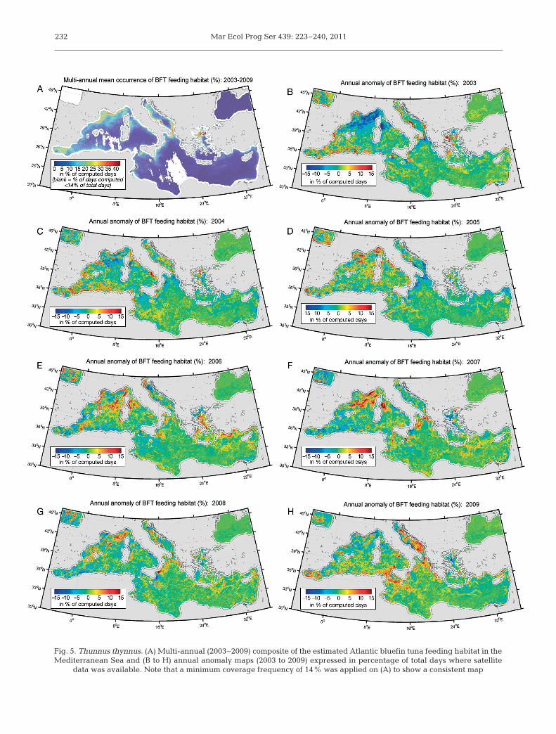
defined areas, such as the Alboran Sea, the Gulf ofLions, the Ligurian Sea, the southern Adriatic Seaand the northern Aegean Sea (Fig. 5A). In contrast,the Tyrrhenian Sea and most of the central andsouthern part of the eastern Mediterranean Seashowed a low occurrence of potential forage habitat(<5% of the time). Whereas the feeding habitat wasconcentrated on the edge of the basin, the mainpotential spawning grounds (>1.6% of the time,Fig. 6A) were mostly in the central parts of the west-ern Mediterranean Sea (around the Balearic Islandsand Sardinia as well as north of the Algerian andSicilian coasts) and in the Gulf of Syrta, east of Sicily,the central Aegean Sea and the northern LevantineSea. Note that there is little overlap between bothhabitats. While the feeding habitat was rather contin-uous and stretched out, the spawning habitat waspatchier with a round shape. This is understandableas the feeding grounds are mostly influenced by thegeneral circulation, while the spawning habitat isprimarily affected by the spring surface heating,which displays a higher year-to-year spatial variabil-ity. From the daily to seasonal time scales (see anom-aly maps, Fig. 6B−H), the integration of SST differ-ences over 30 d emphasizes mostly large andcontinuous patches of potential spawning habitat.

Spatial variability at the annual scale

The computation of annual anomalies of habitatoccurrence compared to the mean value for theperiod 2003−2009 showed that the main spatial pat-terns significantly changed year-to-year (Figs. 4 & 5).For instance, the heatwave during the summer of2003 in Europe is likely to have caused a strongreduction in the feeding habitat of the northwesternMediterranean (except in the Gulf of Lions), while itincreased in the southwestern Mediterranean Sea(from ±5 to ±15%; Fig. 5B). A positive anomaly in thenorthwestern Mediterranean Sea was detected in2005−2008. Even if patterns varied locally, the anom-aly of the feeding habitat from 2003 to 2005 was glob-ally low or negative at the scale of the central andeastern Mediterranean Sea, while it was positive forthe period 2006−2009. The ABFT feeding habitat alsoshows a strong inter-annual variability in the AdriaticSea in 2003 and 2009 with strong anomalies (from 10to 30%) between the northeast Adriatic coastal areaand the central and eastern basin (Fig. 5B,H). Similardifferences between 2003 and 2009 also took place inthe Sicilian Strait, the northern Ionian Sea and west-ern Aegean Sea. The spawning habitat displayed

231

Mar Ecol Prog Ser 439: 223–240, 2011232

Fig. 5. Thunnus thynnus. (A) Multi-annual (2003−2009) composite of the estimated Atlantic bluefin tuna feeding habitat in theMediterranean Sea and (B to H) annual anomaly maps (2003 to 2009) expressed in percentage of total days where satellite

data was available. Note that a minimum coverage frequency of 14% was applied on (A) to show a consistent map

Druon et al.: Bluefin tuna potential habitat mapping in the Mediterranean 233

Fig. 6. Thunnus thynnus. (A) Multi-annual (2003−2009) composite of the predicted Atlantic bluefin tuna spawning habitat inthe Mediterranean Sea and (B to H) annual anomaly maps (2003 to 2009) expressed in percentage of total days where satellite

data was available. Note that a minimum coverage frequency of 28% was applied on (A) to show a consistent map

Mar Ecol Prog Ser 439: 223–240, 2011234

Fig. 7. Thunnus thynnus. (A−D) Seasonal composite of Atlantic bluefin tuna feeding habitat in the Mediterranean Sea for theperiod 2003−2010, as percentage of total days where satellite data was available: (A) winter, (B) spring, (C) summer, (D)autumn. A minimum value of 6% of available data was applied to show consistent maps. (E−H) Mean fortnight composite(2003−2010) of bluefin tuna spawning habitat in the Mediterranean Sea as percentage of total days where satellite data wasavailable: (E) second half of May, (F) first and (G) second half of June, and (H) first half of July. A minimum value of 22% of

available data was applied to show consistent maps

Druon et al.: Bluefin tuna potential habitat mapping in the Mediterranean

even higher year-to-year variations; the most spec-tacular occurring around Sardinia in 2006 (Fig. 6E).This anomaly was supported by unusual purse seinefishing west of Sardinia in June 2006 (J. M. Fro-mentin pers. obs.) as well as the observation ofnumerous ABFT juveniles of ~35 cm in September2006 in the coastal area southeast of Sardinia(P. Addis pers. comm.). In 2003, the spawning habitatdisplayed smaller favourable areas than on averageor in 2006 (Fig. 6B).

Spatial variability at the seasonal scale

Both the feeding and spawning habitats were alsohighly variable between seasons, but these varia-tions were not equally distributed. Regarding thefeeding habitat, the northwestern MediterraneanSea and the Alboran Sea were more dynamic thanthe others, as these key feeding areas were mostlyactive in summer and autumn, while the other keyfeeding grounds (Adriatic Sea and Aegean Sea)appear more stable all year round (Fig. 7A−D). Thesummer and autumn are also characterized by amore concentrated feeding habitat than in winterand spring. The ABFT spawning habitat occurs frommid-May to July following a heating wave and strat-ification build-up from east to west as shown by themean fortnight composites (Fig. 7E−H). Although theinter-annual variability is high (Fig. 6), this longitudi-nal dynamic is recurrent every year.

Main temporal patterns

To better quantify these different sources of varia-tions at the basin scale, we computed the surface ofthe Mediterranean Sea displaying favourable feed-ing or spawning habitats for ABFT for each month ofeach year for the 2003−2009 period (Fig. 8). Regard-ing the feeding habitat, the seasonal cycle was wellmarked with minimum surface values during sum-mer (~5% of the Mediterranean Sea) and maximumsurface values in late autumn (10% of the basin).Year-to-year variations may reach 25 to 35%, butwere less important than the seasonal variation.However, there was no specific trend in the year-to-year variations. Regarding the spawning habitat, theseasonal pattern is even more obvious, as the spawn-ing is strongly restricted in time (i.e. from May toJuly). As expected from the literature, the maximumvalues mostly occurred in June and ranged from4.7% to 8.1% of the Mediterranean Sea (2008 and

2003, respectively). However, the size of spawninghabitat did not always peak in June. In 2009, thelargest areas favourable for spawning took placealmost equally in May and June, while in 2006 itpeaked in July (owing to an unusual extensionaround Sardinia; Fig. 6E). The standard deviation ofthe predicted surface for the spawning habitat wasabout 50 to 65% for the period May to July, twice thatof the feeding habitat. This higher variability isexpected since the former is mainly influenced bymeteorological conditions (stratification build-up)and the latter by a mixed influence of meteorologicalconditions and the general oceanic circulation.

The mean annual values of habitat surfaces for theperiod 2003−2009 were 2 to 3× less variable than themonthly surfaces (results not shown). Similarly, thevariability was higher for the spawning habitat (highin 2003, 2006 and 2009 and low in 2005 and 2008)

235

2

A

B

4 6 8 10 12 143

4

5

6

7

8

9

10

11

12

13

Mo

nth

ly m

ean

sea s

urf

ace o

f th

e

feed

ing

hab

itat

(%)

2003200420052006200720082009mean

2 4 6 8 10 12 140

1

2

3

4

5

6

7

8

9

Month

Mo

nth

ly m

ean

sea s

urf

ace o

f th

e

sp

aw

nin

g h

ab

itat

(%)

Fig. 8. Monthly mean surface (%) of the Mediterranean Seaestimated to be favourable for Atlantic bluefin tuna Thunnusthynnus (A) feeding and (B) spawning from 2003 to 2009 and

for the 2003−2009 period

Mar Ecol Prog Ser 439: 223–240, 2011

than for the feeding habitat (high in 2006, 2007 and2009 and low in 2003). More interestingly, there wasa 6% increase in the surface of the potential feedinghabitat over the period 2003−2009. However, the 7-yrtime series of the present study remains too short toreach any clear conclusion about the variations atlow frequency.

DISCUSSION

Our approach provides, for the first time, a synopticview of the potential feeding and spawning habitatsof ABFT in the Mediterranean Sea as well as theirspatial and temporal variations, which are both cru-cial to evaluate the utility of MPAs or to correct keyinputs in stock assessment models such as the Catchper Unit Effort indices. Nonetheless, this approachhas a few limitations, mostly the cloud cover, and thequantity and distribution (in time and space) of ABFTobservations. Druon (2010) discussed the impact ofcloud cover on the habitat coverage in the Mediter-ranean Sea, which is seasonal (maximum in winterand minimum in summer). For instance, for the years2006 and 2007, the mean annual habitat coveragewhen computing the daily feeding habitat of 22 ± 6%of the Mediterranean Sea is lower than that of theperiod from May to July with a value of 29 ± 8%. Forcomparison with the feeding habitat, the mean habi-tat coverage when computing the spawning habitatfrom May to July is significantly higher with a valueof 55 ± 14%. For operational use, the 3-day compos-ite habitat map is therefore fairly well covered duringthe spawning (and currently fishing) season. We alsoinvestigated the use of other sensors for SST andCHL in parallel, i.e. MODIS-Terra for NSST and Sea-WiFS for CHL, which lag 3 and 1.5 h behind MODIS-Aqua, respectively. The mean increase of habitatcoverage due to changes in cloud coverage whenusing both pairs of sensors was 13% for the spawninghabitat and 36% for the feeding habitat in 2003(Aulanier & Druon 2010). When the model was cali-brated using only SeaWiFS/MODIS-Terra, there waslittle difference in habitat classification (5% for feed-ing and 11% for spawning) from that with the cali-bration based on MODIS-Aqua. This indicates thatthe data from both sensors could be used in parallel(Aulanier & Druon 2010). Although this approachneeds to be confirmed with additional ABFT obser-vations, the combination of several satellite sensorsappears to be a promising approach to partially cir-cumvent the difficulties induced by cloud cover. Theuse of smoother and cloud free SST data, such as pro-

posed by GHRSST (https://www.ghrsst.org/), couldimprove the signal:noise ratio by removing a propor-tion of high frequency noise that can be observed inthe potential spawning habitat when computing the30 d gradient. This needs to be further explored onABFT, but also on other species for which the SSTcoverage is poorer, such as tropical tuna species.However, the lack of ABFT observations and the highcloud coverage during winter in the western andcentral Mediterranean Sea as well as the low numberof ABFT observations in the eastern MediterraneanSea remain the most prominent technical limitationsof our current approach.

One might question what potential habitat repre-sents compared to effective habitat. Most of the cur-rent habitat models (Barry & Elith 2006) or catch−effort standardization for fish stock assessments(Maunder & Punt 2004) rely on statistical approaches(e.g. regression models such as generalized linear oradditive models) where correlation or co-occurrenceis examined between the targeted species and envi-ronmental variables. However, such approaches alsodisplay some limitations, e.g. in some cases theabsence of the given species remains uncertain (e.g.for marine mammals) and biases can be introduceddue to the lack of homogeneous distribution of thepopulation in the area of interest. Moreover, theabsolute values of environmental variables at theposition of the occurrence of the species might be notrelevant, because large pelagic species, such asABFT, albacore tuna, right or rorqual whales, seem toseek specific oceanic features showing high horizon-tal gradients such as fronts (see e.g. Royer et al. 2004,Schick et al. 2004, Stokesbury et al. 2004, Zainuddinet al. 2006, Doniol-Valcroze et al. 2007, Rooker et al.2008, Pershing et al. 2009, Lawson et al. 2010). This isin line with Barry & Elith (2006) when reviewingerrors and uncertainties of species distribution mod-els, who concluded that the most robust modellingapproaches are likely to be those in which care istaken to match the model with knowledge of ecology.Therefore, we believe that the potential habitat, asdefined in this study, better describes the functionalhabitat than standard GLM or GAM approaches,especially for highly migratory species which spenda significant time searching for favourable areas fortheir reproduction. Because the potential habitat isdefined by oceanic features, it was necessary todefine its size using the factor Wf in the cost functionfmin (see ‘Methods: Calibration of the habitat model’)and we found an optimal extension. This parameteris likely to include several characteristics, such as thedistance covered by the target species per time unit,

236

Druon et al.: Bluefin tuna potential habitat mapping in the Mediterranean

the quantity and quality of environmental informa-tion collected and the fish or school behaviour.Therefore, this parameter is likely to be species- specific. Since the potential habitat is traced bymeso-scale oceanic structures close to (but notdirectly by) ABFT presence, a single observation maychange habitat classification depending on therespective size of each habitat (driven by the respec-tive parameterization). In fact, while processing dif-ferent calibration runs, a few observations (<5%)changed habitat classification in areas where feedingand spawning habitats are close to each other (in theBalearic Islands area).

Emphasis was placed on the use of relative satellitedata (computation of spatial and temporal gradients)with a minor contribution of absolute values whichare less consistent. As mentioned above, satellite-derived SST and CHL data are influenced by specificmeasurement characteristics (water depth and at -mos pheric influence, respectively) leading to higheruncertainties in the absolute values compared tofield measurements. However, the variability atmeso-scale and over several weeks indicates thatsatellite data adequately describe the oceanic fea-tures. The spatial resolution of 4.6 km appears to berelevant to detect oceanic features of importance forABFT. The use of the original (non geo-projected)data at 1 km resolution is likely to allow a slightimprovement in the model performances and wouldallow accessing the potential feeding habitat closerto the coast (~3 km vs. ~15 km currently). However,this would also notably impede progress in themethodology by increasing the computing time for aminor benefit.

The present model performs well in areas whereboth satellite data and ABFT observations are avail-able. Indeed, (1) a large fraction of ABFT observa-tions are in the vicinity of the potential habitat (over-all, 80% of observations are within 9.0 km of apotential habitat, n = 430), (2) the general shapes ofthe histograms of ABFT occurrences against dis-tances from the habitat boundary are very satisfac-tory, (3) the validation with an independent datasetclearly supports the former calibration of the model,(4) further tests showed that potential habitat fittedfrom ABFT geo-located observations is notably dif-ferent from the one that could be obtained with ran-dom data and (5) the information on fish weight thatis not used in the habitat model is in agreement withthe model results, as adult ABFT (i.e. fish weight>30 kg) were mostly found within the potentialspawning habitat during the spawning season, whilejuveniles (i.e. fish weight <30 kg) were mostly found

close to the potential feeding habitat. Therefore, itcould be of interest to obtain access to a largerdataset on ABFT to test whether the characteristicsand spatial distribution of the feeding habitat wouldchange when a larger proportion of adult fish is con-sidered. It is also worth noting that the general loca-tions of potential feeding and spawning habitats thathave been detected in the Mediterranean Sea by ourmodel are in good agreement with current knowl-edge (Mather et al. 1995, Fromentin & Powers 2005,Rooker et al. 2007). Furthermore, the general timingof the spawning as well as the east−west sequence offavourable spawning habitat in the MediterraneanSea from mid-May to mid-July is also correctly esti-mated by the model. This result is in agreement with(1) studies on ABFT gonadosomatic index wheremaximum values were found in late May and earlyJune in the Levantine Sea (eastern MediterraneanSea), and 2 and 4 wk later in the central (Malta) andwestern (Balearic Islands) locations, respectively(Heinisch et al. 2008) and (2) the general movementof the purse seine fleet tracking ABFT spawners thatstart fishing in the Eastern Mediterranean in Mayand end in July in the Balearic Islands area. The out-puts that are not fully supported by current knowl-edge mostly concern the spawning habitat, espe-cially the areas of the Ligurian Sea, east of Sicily andthe northern Aegean Sea. Regarding the Ionian Seaarea east of Sicily, the model identified an importantpotential spawning habitat which is in accordancewith the reported occurrence of ABFT larvae in thatarea (Rooker et al. 2007). Catches of large individuals(spawners) in the Gulf of Syrta since 2002 werereported in May and June which suggest that thisarea could be a key spawning ground, although fewABFT larvae have been reported. The importance ofthe potential feeding and spawning habitat in theAegean Sea also appears to be disproportionate, con-sidering current knowledge and the low occurrenceof commercial fleets in this area. However, the poten-tial spawning habitat in this area is mainly inferredover the 2003−2009 period by the event of 2008(Fig. 6G). The purse seine fleet was also twice as effi-cient in fishing in spawning grounds as in feedinggrounds (Druon 2010) and a significant number ofpop-up positions from electronic tags are reported inthe Aegean Sea compared to the rest of the Mediter-ranean Sea (De Metrio et al. 2005, review in Rookeret al. 2007). However, no satisfactory explanation hasbeen found for the remaining problematic area, thenorthern Ligurian Sea. This problem might revealsome limitations in the current model, especially thelack of one or more covariates to specify the spawn-

237

Mar Ecol Prog Ser 439: 223–240, 2011

ing habitat, such as currents. Another im provementof the method for the potential feeding habitat wouldbe to estimate the age of frontal structures in order toretain only features old enough (~2 wk) to sustain thedevelopment of micro-zoo plankton, which in turnattracts higher-level pre dators. Additional informa-tion of ABFT spatial distribution needs to be col-lected, especially from current electronic taggingexperiments in the Mediterranean Sea (Fromentin2010), to help us to distinguish between possible spu-rious predictions of habitat and incomplete knowl-edge. Nevertheless, the general consistency of themodel outputs with current knowledge clearly indi-cates that defining a potential habitat on a given setof oceanographic structures appears to be relevantfor ABFT.

The application of this methodology on ABFTreveals other patterns of interest. The feeding habitatdisplays a stretched shape while the spawning habi-tat is patchier. Depending on the occurrence and sizeof each pattern type, it could be worth investigatingwhether the geometrical aspect has an impact on thecapacity of the species to find its favourable habitat.If most of the feeding and spawning grounds are inagreement with current knowledge, the presentstudy further shows large spatial and temporal varia-tions in both habitats at both the seasonal and annualscales (thanks to the high temporal and spatial reso-lution of remote-sensing data). This result, which isin agreement with local observations from scientistsor fishermen, is of particular interest as it embraces,for the first time, a synoptic view of the entireMediterranean Sea over 7 continuous years. Thus,this approach can detect special features, such as thelow occurrence of potential feeding habitat in theMediterranean Sea in 2003 or the unusually strongoccurrence of potential spawning habitat aroundSardinia in 2006 (the latter being supported by fish-eries information and the high abundance of smallABFT southeast of Sardinia 2 mo later).

Such unusual events shed light on key biologicaland ecological processes. The 2006 Sardinian epi -sode as well as the general spatial variability in thepotential spawning habitat would indeed advocatespatial learning, rather than imprinting, whenexplaining the underlying mechanisms of ABFThoming (Fromentin & Powers 2005). It would beworth sampling (including with electronic tags) thatarea to investigate whether ABFT born in 2006return during June−July in subsequent years. Over-all, the high seasonal and annual variability in poten-tial habitats that we detected is in agreement withthe outputs from electronic tagging, which empha-

sizes high variations in migratory behaviour amongindividuals in terms of both season and year (e.g.Block et al. 2005, Sibert et al. 2006b, Galuardi et al.2010). Similarly, the analyses of long-term fisheriesdata have already put forward the key role ofchanges in ABFT migration patterns to explain thelong-term fluctuations in trap catches (Ravier & Fro-mentin 2001, 2004) as well as the appearance anddisappearance of key ABFT fishing grounds duringthe 20th century (Tiews 1978, Mather et al. 1995, Fro-mentin 2009). Thus our study shows that changes inABFT migration patterns could be related to naturalvariations in their feeding and spawning habitats,but analysis of the key role of prey distribution vari-ability was beyond the scope of this study.

Finally, mapping potential fish habitats may have apossible role in the spatial management and the con-trol of fisheries, as this has been already shown forthe Chilean anchovy, southern bluefin tuna andswordfish (see Yáñez et al. 2004, Hobday & Hart-mann 2006, Hobday et al. 2010). The near real-timemaps have also been recently proposed for ABFT todefine open and closed fishing areas or to enforcecontrols at sea (Casey et al. 2009, Druon 2010). Thecomposites over a decade may also be useful todefine essential habitats requiring protection, prefer-ably through a web of MPAs. This generic approachcan be transposed a priori to other pelagic species(e.g. other pelagic tuna, small pelagic, and shallowdemersal fish). The approach has also been success-fully applied on the finback whale Balaenopteraphysalus (potential feeding habitat only) in the Medi -terranean Sea with similar performances (Druon etal. unpubl.). This top predator, which mainly feeds onkrill in this area, displays a feeding habitat that iswell defined by frontal structures. This gives furthersupport to the key role of the frontal systems in theproductivity of the Mediterranean Sea. Chl a frontsare indeed sufficiently persistent to sustain a com-plete food web starting with micro- zooplankton.Planktonic feeders, such as anchovy and sardine, aretherefore likely to also be related to these productivefrontal systems while being a prey for ABFT (Royer etal. 2004, Schick et al. 2004). We now plan to applyour approach of using earth ob servation data to de -scribe potential habitat for anchovy, hake and tropi-cal pelagic tunas (skipjack and yellowfin tunas).

Acknowledgements. The authors thank the Ocean BiologyProcessing Group (Code 614.2) at the GSFC, Greenbelt, MD20771, for the efficient production and distribution of oceancolour and sea surface temperature data. The authors areespecially grateful to R. Delponte who provided a significantfraction of ABFT sightings from his logbooks as well as Ifre-

238

Druon et al.: Bluefin tuna potential habitat mapping in the Mediterranean 239

mer for the field campaigns targeting ABFT. We are thank-ful for valuable comments and suggestions provided by 4anonymous reviewers and the subject editor. We alsoexpress our gratitude to E. MacAoidh for correcting the English.

LITERATURE CITED

Aulanier F, Druon JN (2010) Habitat modelling of marinespecies derived from satellite data: technical aspects.European Commission EUR 24498 EN — Scientific andTechnical Research series — Joint Research Centre. Pub-lications Office of the European Union, Luxembourg

Bard FX, Bach P, Josse E (1998) Habitat et écophysiologiedes thons: Quoi de neuf depuis 15 ans? Collect Vol SciPap ICCAT 50: 319−342

Barry S, Elith J (2006) Error and uncertainty in habitat mod-els. J Appl Ecol 43: 413−423

Beddington JR, Agnew DJ, Clark CW (2007) Current prob-lems in the management of marine fisheries. Science316: 1713−1716

Block BA, Teo SLH, Walli A, Boustany A and others (2005)Electronic tagging and population structure of Atlanticbluefin tuna. Nature 434: 1121−1127

Bonhommeau S, Farrugio H, Poisson F, Fromentin JM (2010)Aerial surveys of bluefin tuna in the western Mediter-ranean Sea: retrospective, prospective, perspectives.Collect Vol Sci Pap ICCAT 65:801–811

Brill R, Lutcavage M, Metzer G, Bushnell P and others (2002)Horizontal and vertical movements of juvenile bluefintuna (Thunnus thynnus, in relation to oceanographicconditions of the western North Atlantic, determinedwith ultrasonic telemetry. Fish Bull 100: 155−167

Casey J, Vanhee W, Druon JN (eds) (2009) Advice on stocksof interest to the European Community in areas underthe jurisdiction of CCAMLR, CECAF, WECAF, ICCAT,IOTC, IAATC, GFCM, NAFO, and stocks in the NorthEast Atlantic. Report of the European Scientific, Techni-cal and Economic Committee for Fisheries, Vigo, Spain,19−23 October 2009. EC Joint Research Centre, Brussels.http://stecf.jrc.ec.europa.eu/c/document_library/get_file?p_l_id=53322&folderId=44863&name=DLFE-4716.pdf

Connor DW, Gilliland PM, Golding N, Robinson P, Tod D,Verling E (2006) UKSeaMap: the mapping of seabed andwater column features of UK seas. Joint Nature Conser-vation Committee, Peterborough. www.vliz.be/imisdocs/publications/125357.pdf

de Juan S, Lleonart J (2010) A conceptual framework for theprotection of vulnerable habitats impacted by fishingactivities in the Mediterranean high seas. Ocean CoastManage 53: 717−723

De Metrio G, Arnold GP, de la Serna JM, Block BA and oth-ers (2005) Movements of bluefin tuna (Thunnus thynnusL.) tagged in the Mediterranean Sea with pop-up satel-lite tags. Collect Vol Sci Pap ICCAT 58: 1337−1340

Doniol-Valcroze T, Berteaux D, Larouche P, Sears R (2007)Influence of thermal fronts on habitat selection by fourrorqual whale species in the Gulf of St. Lawrence. MarEcol Prog Ser 335: 207−216

Druon JN (2010) Habitat mapping of the Atlantic bluefintuna derived from satellite data: Its potential as a tool forthe sustainable management of pelagic fisheries. MarPolicy 34: 293−297

Fromentin JM (2009) Lessons from the past: investigating

historical data from bluefin tuna fisheries. Fish Fish 10: 197−216

Fromentin JM (2010) Tagging bluefin tuna in the Mediter-ranean Sea: challenge or mission impossible? Collect VolSci Pap ICCAT 65: 812−821

Fromentin JM, Powers JE (2005) Atlantic bluefin tuna: pop-ulation dynamics, ecology, fisheries and management.Fish Fish 6: 281−306

Fromentin JM, Restrepo V (2001) Recruitment variabilityand environment: Issues related to stock assessments ofAtlantic tunas. Collect Vol Sci Pap ICCAT 52: 1780−1792

Fromentin JM, Farrugio H, Deflorio M, De Metrio G (2003)Preliminary results of aerial surveys of bluefin tuna in thewestern Mediterranean Sea. Collect Vol Sci Pap ICCAT55: 1019−1027

Galuardi B, Royer F, Golet W, Logan J, Neilson J, LutcavageM (2010) Complex migration routes of Atlantic bluefintuna (Thunnus thynnus) question current populationstructure paradigm. Can J Fish Aquat Sci 67: 966−976

García A, Alemany F, Velez-Belchí P, Jurado JLL and others(2005) Characterization of the bluefin tuna spawninghabitat off the Balearic Archipelago in relation to keyhydrographic features and associated environmentalconditions. Collect Vol Sci Pap ICCAT 58: 535−549

Garcia A, Alemany F, Velez-Belchi P, Lopez Jurado JL andothers (2006) Characterization of the bluefin tuna spawn-ing habitat off the Balearic archipelago in relation tokey hydrographic features and associated environmentalconditions. ICCAT, SCRS/2003/76

Halpern BS, Warner RR (2002) Marine reserves have longand lasting effects. Ecol Lett 5: 361−366

Heinisch G, Corriero A, Medina A, Abascal FJ and others(2008) Spatio-temporal pattern of bluefin tuna (Thunnusthynnus L. 1758) gonad maturation across the Mediter-ranean Sea. Mar Biol 154: 623−630

Hilborn R, Orensanz J, Parma A (2005) Institutions, incen-tives and the future of fisheries. Philos Trans R Soc B 360: 47−57

Hobday AJ, Hartmann K (2006) Near real-time spatial man-agement based on habitat predictions for a longlinebycatch species. Fish Manag Ecol 13: 365−380

Hobday AJ, Hartog JR, Timmiss T, Fielding J (2010)Dynamic spatial zoning to manage southern bluefin tuna(Thunnus maccoyii) capture in a multi species longlinefishery. Fish Oceanogr 19: 243−253

Humston R, Ault JS, Lutcavage M, Olson DB (2000) School-ing and migration of large pelagic fishes relative to envi-ronmental cues. Fish Oceanogr 9: 136−146

ICCAT (2007) Report of the 2006 Atlantic Bluefin Tuna StockAssessment Session. Collect Vol Sci Pap ICCAT 60: 652−880

ICCAT (2009) Report of the 2008 Atlantic Bluefin TunaStock Assessment Session. Collect Vol Sci Pap ICCAT 64: 1−352

Inagake D, Yamada H, Segawa K, Okazaki M, Nitta A, ItohT (2001) Migration of young bluefin tuna, Thunnus ori-entalis Temminck et Schlegel, through archival taggingexperiments and its relation with oceanographic condi-tions in the Western North Pacific. Bull Natl Res Inst FarSeas Fish 38: 53−81

Kitagawa T, Kimura S, Nakata H, Yamada H (2004) Divingbehavior of immature, feeding Pacific bluefin tuna(Thunnus thynnus orientalis ) in relation to season andarea: the East China Sea and the Kuroshio-Oyashio tran-sition region. Fish Oceanogr 13: 161−180

Mar Ecol Prog Ser 439: 223–240, 2011

Larkin PA (1996) Concepts and issues in marine ecosystemmanagement. Rev Fish Biol Fish 6: 139−164

Laurs RM, Fiedler PC, Montgomery DR (1984) Albacoretuna catch distributions relative to environmental features observed from satellites. Deep-Sea Res A 31: 1085−1099

Lawson GL, Castleton MR, Block BA (2010) Movements anddiving behavior of Atlantic bluefin tuna Thunnus thyn-nus in relation to water column structure in the north-western Atlantic. Mar Ecol Prog Ser 400: 245−265

Le Fèvre J (1986) Aspects of the biology of frontal systems.Adv Mar Biol 23: 163−299

Lehodey P, Bertignac M, Hampton J, Lewis A, Picaut J(1997) El Nino Southern Oscillation and tuna in the west-ern Pacific. Nature 389: 715−718

Lioka C, Kani K, Nhhala H (2000) Present status andprospects of technical development of tuna sea-farming.Cah Opt Méditerr 47: 275−285 http: //ressources.ciheam.org/om/pdf/c47/00600628.pdf

Mather FJ, Mason JM Jr, Jones A (1995) Historical docu-ment: life history and fisheries of Atlantic bluefin tuna.NOAA Tech Memo NMFS-SEFSC-370, Miami, FL

Matlab (2006) Matlab R2006a, The language of technicalcomputing, MathWorks, Natick, MA

Maunder MN, Punt AE (2004) Standardizing catch and effortdata: a review of recent approaches. Fish Res 70: 141−159

Munk P, Larsson PO, Danielsen D, Moksness E (1995) Larvaland small juvenile cod Gadus morhua concentrated inthe highly productive areas of a shelf break front. MarEcol Prog Ser 125: 21−30

Nelder JA, Mead R (1965) A simplex method for functionminimization. Comput J 7: 308–313

Nishikawa Y, Honma M, Ueyanagi S, Kikawa S (1985) Aver-age distribution of larvae of oceanic species of scombroidspecies, 1956−1981. Far Seas Fisheries Research Labora-tory Series S 12

Olson DB, Hitchcock GL, Mariano AJ, Ashjian CJ, Peng G,Nero RW, Podesta GP (1994) Life on the edge: marine lifeand fronts. Oceanography 7: 52−60

Pershing AJ, Record NR, Monger BC, Mayo CA and others(2009) Model-based estimates of right whale habitat usein the Gulf of Maine. Mar Ecol Prog Ser 378: 245−257

Polovina JJ, Howell E, Kobayashi DR, Seki MP (2001) Thetransition zone chlorophyll front, a dynamic global fea-ture defining migration and forage habitat for marineresources. Prog Oceanogr 49: 469−483

Ravier C, Fromentin JM (2001) Long-term fluctuations in theEastern Atlantic and Mediterranean bluefin tuna popu-lation. ICES J Mar Sci 58: 1299−1317

Ravier C, Fromentin JM (2004) Are the long-term fluctua-tions in Atlantic bluefin tuna (Thunnus thynnus) popula-tion related to environmental changes? Fish Oceanogr13: 145−160

Rooker JR, Alvarado Bremer JR, Block BA, Dewar H andothers (2007) Life history and stock structure of Atlanticbluefin tuna (Thunnus thynnus). Rev Fish Sci 15: 265−310

Rooker JR, Secor DH, DeMetrio G, Kaufman AJ, BelmonteRios A, Ticina V (2008) Evidence of trans-Atlantic move-ment and natal homing of bluefin tuna from stable iso-topes in otoliths. Mar Ecol Prog Ser 368: 231−239

Royer F, Fromentin JM, Gaspar P (2004) Association

between bluefin tuna schools and oceanic features in thewestern Mediterranean. Mar Ecol Prog Ser 269: 249−263

Sammari C, Millot C, Prieur L (1995) Aspects of the seasonaland mesoscale variabilities of the Northern Current inthe western Mediterranean Sea inferred from the PRO-LIG-2 and PROS-6 experiments. Deep-Sea Res I 42: 893−917

Schaefer KM (2001) Reproductive biology of tunas. In: BlockBA, Stevens ED (eds) Tuna physiology, ecology and evo-lution. Academic Press, San Diego, CA, p 225−270

Schick RS, Lutcavage ME (2009) Inclusion of prey dataimproves prediction of bluefin tuna (Thunnus thynnus)distribution. Fish Oceanogr 18: 77−81

Schick RS, Goldstein J, Lutcavage ME (2004) Bluefin tuna(Thunnus thynnus) distribution in relation to sea surfacetemperature fronts in the Gulf of Maine (1994–96). FishOceanogr 13: 225−238

Sibert JR, Lutcavage ME, Nielsen A, Brill RW, Wilson SG(2006a) Interannual variation in large-scale movement ofAtlantic bluefin tuna (Thunnus thynnus) determinedfrom pop-up satellite archival tags. Can J Fish Aquat Sci63: 2154−2166

Sibert J, Hampton J, Kleiber P, Maunder M (2006b) Biomass,size, and trophic status of top predators in the PacificOcean. Science 314: 1773−1776

Stokesbury MJW, Teo SLH, Seitz A, O’Dor RK, Block BA(2004) Movement of Atlantic bluefin tuna (Thunnusthynnus) as determined by satellite tagging experimentsinitiated off New England. Can J Fish Aquat Sci 61: 1976−1987

Sumaila UR, Zeller D, Watson R, Alder J, Pauly D (2007)Potential costs and benefits of marine reserves in thehigh seas. Mar Ecol Prog Ser 345: 305−310

Teo SLH, Boustany A, Dewar H, Stokesbury MJW and others (2007) Annual migrations, diving behavior, andthermal biology of Atlantic bluefin tuna, Thunnus thyn-nus, on their Gulf of Mexico breeding grounds. Mar Biol151: 1−18

Tiews K (1978) On the disappearance of bluefin tuna in theNorth Sea and its ecological implications for herring andmackerel. Rapp P-V Reùn Cons Int Explor Mer 172: 301−309

Ullman DS, Cornillon PC (2000) Evaluation of front detec-tion methods for satellite-derived SST data using in situobservations. J Atmos Ocean Technol 17: 1667−1675

Uotani I, Saito T, Hiranuma K, Nishikawa Y (1990) Feedinghabit of bluefin tuna Thunnus thynnus larvae in thewestern north Pacific Ocean. Bull Jpn Soc Sci Fish 56: 713−717

Walli A, Teo SLH, Boustany A, Farwell CJ and others (2009)Seasonal movements, aggregations and diving behaviorof Atlantic bluefin tuna (Thunnus thynnus) revealed witharchival tags. PLoS ONE 4: e6151

Yáñez E, Silva C, Nieto K, Barbieri MA, Martínez G (2004)Using satellite technology improve Chilean purseinefishing fleet. Gayana 68: 578−585

Zainuddin M, Kiyofuji H, Saitoh K, Saitoh SI (2006) Usingmulti-sensor satellite remote sensing and catch data todetect ocean hot spots for albacore (Thunnus alalunga)in the northwestern North Pacific. Deep-Sea Res II 53: 419−431

240

Editorial responsibility: Konstantinos Stergiou, Thessaloniki, Greece

Submitted: November 26, 2010; Accepted: July 26, 2011Proofs received from author(s): September 30, 2011