NBER WORKING PAPER SERIES

POST-1500 POPULATION FLOWS AND THE LONG RUN DETERMINANTS OFECONOMIC GROWTH AND INEQUALITY

Louis PuttermanDavid N. Weil

Working Paper 14448http://www.nber.org/papers/w14448

NATIONAL BUREAU OF ECONOMIC RESEARCH1050 Massachusetts Avenue

Cambridge, MA 02138October 2008

We thank Charles Jones, Oded Galor and seminar participants at Brown University, the NBER SummerInstitute, the Stockholm School of Economics, The CEGE annual conference at the University of Californiaat Davis, and University College London for helpful comments. We also thank Federico Droller, BryceMillett, Momotazur Rahman, Isabel Tecu, Ishani Tewari, Yaheng Wang, and Joshua Wilde for valuableresearch assistance. The views expressed herein are those of the author(s) and do not necessarily reflectthe views of the National Bureau of Economic Research.

NBER working papers are circulated for discussion and comment purposes. They have not been peer-reviewed or been subject to the review by the NBER Board of Directors that accompanies officialNBER publications.

© 2008 by Louis Putterman and David N. Weil. All rights reserved. Short sections of text, not to exceedtwo paragraphs, may be quoted without explicit permission provided that full credit, including © notice,is given to the source.

Post-1500 Population Flows and the Long Run Determinants of Economic Growth and InequalityLouis Putterman and David N. WeilNBER Working Paper No. 14448October 2008,Revised October 2009JEL No. F22,N30,O40

ABSTRACT

We construct a matrix showing the share of the year 2000 population in every country that is descendedfrom people in different source countries in the year 1500. Using this matrix, we analyze how post-1500migration has influenced the level of GDP per capita and within-country income inequality in the worldtoday. Indicators of early development such as early state history and the timing of transition to agriculturehave much better predictive power for current GDP when one looks at the ancestors of the peoplewho currently live in a country than when one considers the history on that country’s territory, withoutadjusting for migration. Measures of the ethnic or linguistic heterogeneity of a country’s current populationdo not predict income inequality as well as measures of the ethnic or linguistic heterogeneity of thecurrent population’s ancestors. An even better predictor of current inequality in a country is the varianceof early development history of the country’s inhabitants, with ethnic groups originating in regionshaving longer histories of agriculture and organized states tending to be at the upper end of a country’sincome distribution. However, high within-country variance of early development also predicts higherincome per capita, holding constant the average level of early development.

Louis PuttermanDepartment of EconomicsBrown University64 Waterman StreetProvidence, RI 02912Louis_Putterman@brown.edu

David N. WeilDepartment of EconomicsBox BBrown UniversityProvidence, RI 02912and NBERdavid_weil@brown.edu

2

Economists studying income differences among countries in the world today have been increasingly drawn to examine the influence of long-term historical factors. While the theories underlying these analyses vary, the general finding is that things that were happening 500 or more years ago matter for economic outcomes today. Hibbs and Olsson (2004) and Olsson and Hibbs (2005), for example, find geographic factors that predict the timing of the Neolithic revolution in a country also predict income and the quality of institutions in 1997. Comin, Easterly, and Gong (2006, 2009) show that the state of technology in a country 500, 1500, or even 3000 years ago has predictive power for the level of output today. Bockstette, Chanda and Putterman (2002) find that an index of the presence of state-level political institutions from year 1 to 1950 has positive correlations, significant at the 1% level, with both 1995 income and 1960-95 income growth. And Galor and Moav (2007) provide empirical evidence for a link from the timing of the transition to agriculture to current variations in life expectancy. Examining this sort of historical data immediately raises a problem, however: the further back into the past one looks, the more the economic history of a given place tends to diverge from the economic history of the people who currently live there. For example, the territory that is now the United States was inhabited in 1500 largely by hunting, fishing, and horticultural communities with pre-iron technology, organized into relatively small, pre-state political units.1 By contrast, a large fraction of current U.S. population is descended from people who in 1500 lived in settled agricultural societies with advanced metallurgy, organized into large states. The example of the United States also makes it clear that, because of migration, the long-historical background of the people living in a given country can be quite heterogeneous. This observation, combined with the finding that long-history of a country’s residents affects the average level of income, naturally raises the question of whether heterogeneity in background of a country’s residents is a determinant of income inequality within the country. Previous attempts to deal with the impact of migration in modifying the influence of long-term historical factors have been somewhat ad hoc. Hibbs and Olsson, for example, acknowledge the need to account for the movement of peoples and their technologies, but do so only by treating four non European countries (Australia, Canada, New Zealand and the U.S.) as if they were in Europe. Comin, Easterly, and Gong (2006) similarly add dummy variables to their regression model for countries with “major” European migration (the four mentioned above) and “minor” European migration (mostly in Latin America).2 In other cases, variables meant to measure other things may in fact be proxying for migration. For example, the measure of the origin of a country’s legal systems examined by La Porta et al. (1998) may be proxying for the origins of countries’ people. This is also true of Hall and Jones’s (1999) proportion speaking European languages measure. The apparent effect of institutions that were either brought along by European settlers or imposed by non-settling colonial powers, as found in Acemoglu,

1 Anthropologists subscribing to cultural evolutionary models speak of political institutions evolving from the band to the tribe to the chiefdom and finally the state (see, for instance, Johnson & Earle, 1987). There were no pre-Columbian states north of the Rio Grande, according to such schema. 2 Comin, Easterly, and Gong use this technique in their 2006 working paper. In the 2009 version of the paper, they adjust for migration using Version 1.0 of our migration matrix.

3

Johnson, and Robinson (2001, 2002), may be proxying for population shifts themselves, despite their attempt (discussed below) to control for the European-descended population share. In this paper we pursue the issue of migration’s role in shaping the current economic landscape in a much more systematic fashion than previous literature. We construct a matrix detailing the year-1500 origins of the current population of almost every country in the world. (Throughout the paper, we use the term “migration” to refer to any movement of population across current nation borders, although we are cognizant that these movements included transport of slaves and forced relocation as well as voluntary migration.) We then use this matrix as a tool to examine how early development and the pattern of population movements across borders have impacted current income and inequality.

The most thorough previous work along these lines is in the papers by Acemoglu, Johnson, and Robinson (AJR) mentioned above, where they calculate the share of the population that is of European descent for 1900 and 1975. There are a number of conceptual and operational differences between our approach and theirs. Our estimates break down ancestor populations much more finely than “European” and “non-European.” This distinction is important both in the Americas, where there is great variation in the fraction of the population descended from Amerindians vs. Africans, and also in other regions, where important non-native populations are not descended from Europeans (consider the large Chinese-descended populations in Singapore and Malaysia, or Indian descendants in South Africa, Malaysia, and Fiji). Even when we use our matrix to construct a measure of the European population fraction, there are considerable differences between our data and AJR’s. They use as their measure of the European population the fraction of people who are “white,” while we also include an estimate of the fraction of European ancestors among mestizo populations. In Mexico, for example, AJR estimate the European population in 1975 to be 15%, even though (in their data) there is an additional 55% of the population that is mestizo. Our estimate of the European share of ancestors for today’s Mexicans is 29%. The AJR estimates are primarily based on data in McEvedy and Jones (1978), which sometimes apply to whole regions, and occasionally involve extrapolation from as far in the past as 1800. Our data are based on a broader selection of more recent sources, including genetic analyses, encyclopedias, government reports, and compilations by religious groups, which are summarized in Appendices A and B. The correlation between our measure of the European fraction and the AJR measure is 0.89.3

3 The largest differences occur in the Americas. For example, for the five Central American

countries of El Salvador, Nicaragua, Panama, Costa Rica, and Honduras, AJR use a uniform value of 20% European; our estimates range from 45% in Panama to 60% in Costa Rica. The largest outlier in the other direction is Trinidad and Tobago, which they list as 40% European and is only 7% in our measure. Here they seem to have erroneously counted all non-Africans as European, despite the presence of a large Asian population.

4

The rest of this paper is structured as follows. Section 1 describes the construction of our migration matrix, and then uses the matrix to lay out some of the important facts regarding the population movements that have reshaped genetic and cultural landscapes in the world since 1500. We find that a significant minority of the world’s countries have populations mainly descended from the people of other continents and that these countries themselves are quite economically heterogeneous. In Section 2, we apply our migration matrix to analyze the determinants of current income. Using several measures of early development, we show that adjusting the data to reflect where people’s ancestors came from improves the ability of measures of early social and technological development to predict current levels of income. The positive effect of ancestry-adjusted early development on current income is robust to the inclusion of a variety of controls for geography, climate, and current language. We also examine the effect on current income of heterogeneity in early development. We find that, holding constant the average level of early development, heterogeneity in early development raises current income, a finding that might indicate spillovers of growth-promoting traits among national origin groups. In Section 3, we turn to the issue of inequality. We show that heterogeneity in the early development of a country’s ancestors predicts current income inequality and that this effect is robust to the inclusion of several other measures of the heterogeneity of the current population. We also show that ethnic groups originating in regions with higher levels of early development tend to be placed higher in a recipient country’s income distribution. Section 4 concludes. 1. Large-scale population movements since 1500 We use the year 1500 as a rough starting point for the era of European colonization of the other continents. It is well known that most contemporary residents of countries such as Australia and the United States are not descendants of their territory’s inhabitants circa 1500, but of people who arrived subsequently from Europe, Africa, and other regions. But exactly what proportions of the ancestors of today’s inhabitants of each country derive from what regions and from the territories of which present-day countries has not been systematically studied. Accordingly, we examined a wide array of secondary compilations to form the best available estimates of where the ancestors of the long-term residents of today’s countries were living in 1500. Generally, these estimates have to work back from information presented in terms of ethnic groupings in modern populations. For example, sources roughly agree on the proportion of Mexico’s population considered to be mestizo, that is having both Spanish and indigenous ancestors, on the proportion having exclusively Spanish ancestors, on the proportion exclusively indigenous, and on the proportion descended from migrants from other countries. There is similar agreement about the proportion of Haitians descended from African slaves, the proportion of people of (east) Indian origin in Guyana, the proportion of “mixed” and “Asian” people in South Africa, and so on. A crucial and challenging piece of our methodology is the attribution, with proper weights, of mixed populations such as mestizos and mulattoes to their original source countries. Saying, for example, that Mexican mestizos are descended from Spanish

5

immigrants and native Mexicans gives no information about the shares of these different groups in that ancestry. Socially constructed descriptions of race and ethnicity may differ from the mathematical contributions to individuals’ ancestry in which we are interested. Contributions from particular groups may be suppressed, exaggerated, or simply forgotten. For these reasons, whenever possible we have used genetic evidence as the basis for dividing the ancestry of modern mixed groups that account for large fractions of their country’s population.4 The starting point for this analysis is differences in the frequency with which different alleles (alternative DNA sequences at a fixed position on a chromosome) appear in ancestor populations from different parts of the world. Comparing the allele frequency in a modern population to the frequency in source populations, one can derive an estimate of the percentage contribution of each source. Early studies in this literature used blood group frequencies in modern populations to estimate ancestry. More recent studies use allele frequencies for multiple genes. In selecting among studies, we favored those based on larger samples with well-identified source populations as well as those done in more recent years using modern techniques.5 The genetic studies we consulted were sometimes of specific groups (such as mestizos) and sometimes of the population as a whole, unconditional on race or ethnicity. In the former case, we applied the genetic evidence to divide up ancestry in the particular mixed group, and multiplied by that group’s representation in the overall population.6

Examination of this genetic evidence produced a number of surprises regarding the ancestry of new-world populations. For example, the usual historical narrative is that many native populations in the Caribbean, such as the Arawak who occupied the island of Hispaniola (present day Haiti and Dominican Republic), died out during the early decades of colonial rule due to disease and the effects of enslavement. However, genetic evidence suggests that of the ancestors of current residents of the Dominican Republic alive in 1500, 3.6% were local Amerindians. In the case of Costa Rica, 86.5% of residents describe themselves as being of Spanish origin, but genetic evidence (unconditional on ethnicity or race) shows Costa Rican’s ancestry (apart from a small Chinese minority) to be 61% Spanish, 30% Amerindian, and 9% African. A final

4 By “substantial,” we mean 30% or greater. In addition, we incorporated findings from genetic studies on U.S. African-Americans and on Puerto Ricans and Costa Ricans of primarily Spanish descent, for whom modern genetic studies indicate appreciable admixture (with Europeans and Amerindians, respectively) since 1500. 5 We focus on autosomal DNA, which is not sex linked, in preference to information on either the Y chromosome, indicating descent along the male line, or mitochondrial DNA, which indicates descent along the female line. However, evidence from sex-linked genes can provide a useful check on our historical understanding. For example, among many mixed populations in the Caribbean, Native American characteristics are far more common in mitochondrial DNA than on Y chromosomes, indicating that native men were largely unable to breed, while native women produced children with European and African men. 6 We used genetic evidence in our analyses of Belize, Bolivia, Brazil, Cape Verde, Chile, Colombia, Costa Rica, Cuba, Dominican Republic, Ecuador, Guatemala, Mexico, Nicaragua, Paraguay, Peru, Puerto Rico, United States, and Venezuela. We also searched for genetic data for other countries for which our conventional sources list large mixed ancestry populations, but were unsuccessful in finding anything in the cases of El Salvador, Honduras, and Panama. See section II.4 of the Main Appendix as well as the individual country entries in the regional appendices for details.

6

example: the genetic data we examined show a significant contribution of Africans (10%) to the ancestry of the mestizos who make up 60% of Mexico’s population.

In cases where genetic evidence on the ancestry of mixed groups was not available, we relied on textual accounts and/or generalizations from countries with similar histories for which genetic data were available. Genetic information can only distinguish between broad ancestry groups, such as Africans, Native Americans, and Europeans. Beyond this genetic information, other sources were brought to bear to help in the decomposition of mixed categories. For example, we use an archive on the slave trade to estimate the proportion of slaves in a given region who originated from parts of Africa identifiable with certain present-day countries. We apply estimates of where the world’s Ashkenazi Jews and Gypsies lived in 1500 to map people with these ethnic identifications to specific countries of today. Similarly, in some countries such as the United States and Canada, national censuses contain information on the breakdown by specific country of ancestry. Using these methods, we constructed a matrix of migration since 1500. The matrix has 165 rows, each for a present-day country, and 172 columns (the same 165 countries plus seven other source countries with current populations of less than one half million.) Its entries are the proportion of long-term residents’ ancestors estimated to have lived in each source country in 1500. Each row sums to one. To give an example, the row for Malaysia has five non-zero entries, corresponding to the five source countries for the current Malaysian population: Malaysia (0.60), China (0.27), India (0.075), Indonesia (0.04) and the Philippines (0.025). 7 The principal diagonal of the matrix provides a quick indication of differences in the degree to which countries are now populated by the ancestors of their historical populations. The diagonal entries for China and Ethiopia (with shares below half a percent being ignored) are 1.0, while the corresponding entries for Jamaica, Haiti and Mauritius are 0.0 and that of Fiji is close to 0.5. In some cases, the diagonal entry may give a misleading impression without further analysis; for example, the diagonal entry for Botswana is 0.31 because only 31% of Botswanans’ ancestors are estimated to have lived in present-day Botswana in 1500, but another 67% were Africans who migrated to Botswana from what is now neighboring South Africa in the 17th and 18th centuries. Figures 1a and 1b are histograms of the proportion of countries and people, respectively, falling into decile bands with respect to the proportion of the current people’s ancestors residing in the same or an immediate neighboring country in 1500.8 The figures show bimodal distributions, with 9.7% of countries having 0 to 10% indigenous or near-indigenous ancestry and 70.3% of countries having 90 to 100% such

7 The entire matrix and all appendices can be downloaded at http://www.econ.brown.edu/fac/Louis_Putterman/ . Appendix A to this paper briefly describes our sources and methods. Appendix B provides further details, including summaries of the factors behind the estimate for each row. 8 We define immediate neighbor as sharing a land boundary or being separated by less than 24 miles of water. Data are from Correlates of War Project (2000).

7

ancestry. Altogether, 80.9% of the world’s people (excluding those in the smallest countries, which are not covered) live in countries that are more than 90% indigenous in population, while 10.0% live in countries that are less than 30% indigenous, with the rest (dominated by Central America, the Andes, and Malaysia) falling in between. The compositions of non-indigenous populations are also of interest. The populations of Australia, New Zealand and Canada are overwhelmingly of European origin, while Central American and Andean countries have both large Amerindian and substantial European-descended populations, and Caribbean countries and Brazil have substantial African-descended populations. Guyana, Fiji, Malaysia and Singapore are among those countries with substantial minorities descended from South Asians, while Malaysia and Singapore also have large Chinese-descended populations.9 We illustrate differences both in the proportions of people of non-local descent and in the composition of those people by means of Map 1. Country shading indicates the proportion of the population not descended from residents of the same or immediate neighboring countries. Pie charts, drawn for thirteen macro-regions, show the average proportions descended from European migrants, from migrants (or slaves) from Africa, and from migrants from other regions, as well as the proportion descended from people of the same region.10 In terms of territory, about half the world’s land mass (excluding Greenland and Antarctica), comprising almost all of Africa, Europe and Asia, is in countries with almost entirely indigenous populations (shown in black), while about a third has less than 20% indigenous inhabitants, and the remainder, dominated by Central America, the Andes and Malaysia, falls somewhere in between. The heterogeneity of regions in the Americas and Australia/New Zealand is highlighted by the pie charts, showing strong European dominance in Australia/New Zealand, the U.S., Canada, and eastern South America, stronger indigenous presence in the Andes, and strong African representation in the Caribbean. We consider the effects of this heterogeneity in Section 3. While we are mostly interested in using the migration matrix to better understand the determinants of long-run economic performance in countries as presently populated, the versatility of the data can be illustrated by using it to calculate the number of descendants of populations that lived five centuries ago and to see how they’ve fared. Given data on country populations in 2000, the matrix will tell the total number of people

9 The populations of Hong Kong and Taiwan are also overwhelmingly descended from Chinese who came to their territories after 1500, giving those entities 97.1% and 98% ancestry from what is now China, according to the matrix. 10 Regions were defined with the aim of keeping their number small enough for purposes of display and grouping countries with similar population profiles. The Caribbean includes Cuba, Dominican Republic, Haiti, Jamaica, Puerto Rico, and Trinidad and Tobago. Europe is inclusive of the Russian Republic. North Africa, West and Central Asia includes all African and Asian countries bordering the Mediterranean, including Turkey, the traditional Middle East, Afghanistan, and former Soviet republics in the Caucasus and Central Asia. South Asia includes Pakistan, India, Bangladesh, Sri Lanka, Nepal and Bhutan. East Asia includes Mongolia, China, Hong Kong, North and South Korea, Japan, and Taiwan. Southeast Asia includes the remainder of Asia plus New Guinea and Fiji. Note that for calculation of the pie chart shares, ancestors are assumed to be from “the same region” if they are from countries in the regions as thus indicated. This assumption means that Europeans are left out of the “European migrant” category of the pie charts if they live in Europe, even if they’ve migrated within the continent, and likewise for sub-Saharan Africans in SSA.

8

today who are descended from each 1500 source country, and where on the globe they are to be found. For instance, using 2000 population figures from Penn World Tables 6.2, we find that there were 32.9 million descendants of 1500’s Irish alive at the turn of the millennium, of whom 11.3% lived in Ireland itself, 77.2% in the U.S., 5.0% in Australia, and 4.1% in Canada.

Combining the information in the matrix with population data for the years 1500 and 2000 yields a number of interesting insights. Because population data for 1500 are very noisy, particularly at the country level, we confine our analysis to looking at 11 large regions.11 The first two columns of Table 1 list the estimated population of each region in 1500 and 2000. The third column shows the increase in total population over the 500 year period. The primary determinant of this increase in density is the level of economic development in 1500. Europe, East Asia, and South Asia, which were highly developed, had the smallest increases in density. The U.S. and Canada, Australia and New Zealand, and the Caribbean, which were relatively lightly populated, lacked urban centers, and were still home to many pre-agricultural societies in 1500, had the largest increases.12 The next four columns of the table use the matrix to track the relationship between ancestor and descendant populations. In column 4, we calculate the number of descendants per capita for each region in 1500, which can be thought of as a kind of “genetic success” quotient. The lowest values of this measure are in the US and Canada and Australia and New Zealand, where native populations were largely displaced by European colonizers. Among the regions that were relatively developed in 1500, Europe, not surprisingly, has the largest number of descendants per capita. The two regions with the highest genetic success are sub-Saharan Africa and Southeast Asia, which were both relatively poor (and thus less densely populated) in 1500 but in which the native population was hardly at all displaced by migrants. Column 5 calculates the fraction of the current regional population that is descended from the region’s own 1500 ancestors. This ranges from 0.03 for the US and Canada and Australia and New Zealand to almost one for South Asia and East Asia. Column 6 shows the fraction of descendants of the 1500 population that still live in the same region. This is lowest in the Caribbean (38%), Europe (54%), Mexico and Central America (85%) and sub-Saharan Africa (86%). The last column of the table calculates the total number of people descended from a region who live outside it. There were a total of 777 million such people in 2000, amounting to 12.8% of world population. Here Europe is by far the dominant contributor, with 578 million descendents living outside the region, followed by sub-Saharan Africa with 103 million and East Asia with 37 million.13

11 Data are from McEvedy and Jones (1978). The regions are the same as those in Map 1, except that the three parts of South America are collapsed into a single region. 12 Estimates of pre-Columbian population in the Americas are highly controversial due to considerable uncertainty about the death rates in epidemics that followed European contact. Since McEvedy and Jones’s estimates fall toward the low end of some more recent appraisals, the resulting estimates of the increase in population density since 1500 could be overstated. 13 It is worth reminding the reader that we calculate “descendents” by adding up fractions of individuals’ ancestry. Thus two individuals who each have half their ancestry from Europe add up to one descendent in our usage.

9

2. Reassessing the Effects of Early Economic Development 2.1 Measures of Early Development In the introduction, we noted that studies including Hibbs and Olsson (2004, 2005), Comin, Easterly, and Gong (2006) and Chanda and Putterman (2006) find strong correlations between measures of early agricultural, technological, or political development and current levels of economic development, but that these studies make relatively ad hoc adjustments, if any, to account for the large population movements on which this paper focuses. The new migration matrix puts us in a position to remedy these shortcomings and thereby put the theory that very early development persists in its effects on economic outcomes to a more stringent test. We use two measures of early development. The first is an index of state history called statehist. The index takes into account whether what is now a country had present a supra-tribal government, the geographic scope of that government, and whether that government was indigenous or by an outside power. The version used by us, as in Chanda and Putterman (2006, 2007), considers state history for the fifteen centuries to 1500, and discounts the past, reducing the weight on each half century before 1451-1500 by an additional 5%. Let sit be the state history variable in country i for the 50 year period t. sit ranges between 0 and 50 by definition, being 0 if there was no supra-tribal state, 50 if there was a home-based supra-tribal state covering most of the present-day country’s territory, 25 if there was supra-tribal rule over that territory by a foreign power, and taking values ranging from 15 (7.5) to 37.5 (18.75) for home- (foreign-) based states covering between 10 and 50% of the present-day territory or when several small states co-exist on that territory. statehist is computed by taking the discounted sum of the state history variables over the thirty half centuries and normalizing it to be between 0 and 1 (by dividing it by the maximum achievable, i.e. the statehist value of a country that had sit = 50 in each period). In a formula:

statehist = ∑

∑

=

−

=

−

29

0

29

0,

50)05.1(

)05.1(

t

t

tti

t s

For illustration, Ethiopia has the maximum value of 1, China’s statehist value is 0.906 (due to periods of political disunity), Egypt’s value is 0.760, Spain’s 0.562, Mexico’s 0.533, Senegal’s 0.398, and Canada, the U.S., Australia and New Guinea have statehist values of 0.14 14 Bockstette et al. (2002) and Chanda and Putterman (2006) also use versions of statehist that include data for the years between 1501 and 1950. The variable that we call statehist in this paper is the same as what Chanda and Putterman (2006, 2007) call statehist1500. Details on the construction of the state history index, and the data itself, can be found in Putterman (2004). Note that by beginning with 1 C.E., statehist ignores some difference in the onset of state-level society, i.e. those between the most ancient states like Mesopotamia and Egypt (third millennium, B.C.E.), and more recent ones like Rome and pre-Colombian Mesoamerica (first millennium, B.C.E.).

10

Our second measure of early development, agyears, is the number of millennia since a country transitioned from hunting and gathering to agriculture. Unlike a similar measure used by Hibbs and Olsson, which had values for eight macro regions, these data are based on individual country information augmented by extrapolation to fill gaps within regions. The data were assembled by Putterman with Trainor (2006) by consulting region- and country-specific as well as wider-ranging studies on the transition to agriculture, such as MacNeish (1991) and Smith (1995). The variable agyears is simply the number of years prior to 2000, in thousands, since a significant number of people in an area within the country’s present borders are believed to have met most of their food needs from cultivated foods. The highest value, 10.5, occurs for four Fertile Crescent countries (Israel, Jordan, Lebanon and Syria) followed closely by Iraq and Turkey (10), Iran (9.5), China (9) and India (8.5). Near the middle of the pack are countries like Belarus (4.5), Ecuador (4), Ivory Coast (3.5) and Congo (3). At the bottom are countries like Haiti and Jamaica (1) which received crop-growing immigrants from the American mainland only a few hundred years before Columbus, New Zealand (0.8), which obtained agriculture late in the Austronesian expansion, and Cape Verde (0.5), Australia (0.4) and others in which agriculture arrived for the first time with European colonists.15 It is worth noting that while statehist measures a stock of experience with state-level organization that takes into account, for example, set-backs like the disappearance, break-up, or annexation of an existing state by a neighboring empire, agyears simply measures the time elapsed since agriculture’s founding in the country, with no attempt to gauge temporal changes in the kind, intensity, or prevalence of farming within the country’s territory.16

We examine each of these variables both in its original form and adjusted to account for migration. Supposing the “early developmental advantages” proxied by statehist and agyears to be something that migrants bring with them to their new country, the adjusted variables measure the average level of such advantages in a present-day country as the weighted average of statehist or agyears in the countries of ancestry, with weights equal to population shares. For instance, ancestry-adjusted statehist for Botswana is simply 0.312 times the statehist value for Botswana plus 0.673 times statehist for South Africa (referring to the people in South Africa in 1500, not those there presently) plus weights of 0.005 each times the statehist values of France, Germany and the Netherlands (the ancestral homes of Botswana’s small Afrikaner population). Algebraically, the “matrix adjusted” form of any variable is Xv, where X is the migration matrix and v is the variable in its unadjusted form.

Figures 2 and 3 show the effect of this adjustment on the variables statehist and agyears, respectively. The horizontal axis shows the variable in its unadjusted form and the vertical axis shows the variable in its adjusted form. In the case of statehist the data form a sort of check mark: there are a large number of countries along the 45 degree line, where adjusted and unadjusted statehist are the same because there has been little or no in 15 For further description, see Putterman with Trainor (2006). 16 The difference is primarily due to data availability. Accounts of the histories of kingdoms, dynasties, and empires are considerably easier to come by than are detailed agricultural histories.

11

migration. These range from China and Ethiopia, with very high levels of statehist, down to eleven countries at or very near the origin, where there was no history of organized states before 1500 and there has been insignificant migration of people from countries that did have organized states in 1500. There are also a large number of countries along the vertical axis, where a population that had zero statehist has been replaced by migrants who have positive values. There is a great deal of dispersion in the adjusted values of statehist in this group, however, reflecting different mixes of immigrants (primarily European vs. African) and different degrees to which the native population was displaced. Only a handful of countries do not fall into one of these two categories.

In the case of agyears, as show in Figure 3, there are still a lot of countries along

the 45 degree line where there has been no in-migration. However, because almost all countries had a history of agriculture prior to the spread of European colonialization after 1500, there is not the strong vertical element that is seen in Figure 2. In this sense, agyears is clearly picking up a different and prior aspect of early development than is statethist.17

2.2 The Effect of Early Development on Current National Income

Table 2 shows the results of regressing the log of year 2000 per capita income on

our early development measures. Each regression includes the unadjusted form of one early development measure, the adjusted form, or both. Not surprisingly, given previous work, the tests suggest significant predictive power for the unadjusted variables. However, for both measures of early development, adjusting for migration produces a very large increase in explanatory power. In the case of statehist, the R2 goes from .06 to .22, while in the case of agyears it goes from .08 to .24. The coefficients on the measures of early development are also much larger using the adjusted than the unadjusted values. In the third and sixth columns of the table we run “horse race” regressions including both the adjusted and unadjusted measures of early development. We find that the coefficients on the adjusted measures retain their significance and become larger while the coefficients on the unadjusted measures become negative and significant. Before proceeding further we test the robustness of our finding to different indicators of population flows, the addition of controls for geography, and alternative measures of early development. In Table 3, we start by constructing measures of statehist and agyears that are adjusted in the spirit of Hibbs and Olsson (2004, 2005) by simply assigning to four “neo European” countries (the United States, Canada, New Zealand, and Australia) the statehist and agyears values of the United Kingdom.18 As the table shows, these adjusted versions perform better than the unadjusted ones, but not nearly as well as the versions we construct using the migration matrix. When we run

17 Agriculture began in places like the Fertile Crescent, China and Mesoamerica millennia before states arose there, and there are numerous present-day countries, e.g. in the Americas and Africa, on the territories of which agriculture had arisen but states had not as of 1500. 18 Hibbs and Olsson actually assign these countries the values for the region treated as inheriting the Mesopotamian agrarian tradition, which includes all of North Africa, the Middle East and Europe.

12

“horserace” regressions including statehist and agyears adjusted using both our matrix and the “neo Europes” method (columns 2 and 4), the coefficients on the matrix-adjusted measures rise in size and significance, while the coefficient on the “neo Europes” adjusted measures become negative and significant.

We then construct a series of other measures from our matrix. The first is the

fraction of the population made up of “natives” (that is, people whose ancestors lived there in 1500). We include this alongside our measures of adjusted statehist and agyears in order to check that we are not just picking up the fact that there is a correlation between the share of a population’s ancestors who lived elsewhere and the types of countries they lived in. In a similar spirit we construct a measure of the fraction of the descendants of each country’s people in 1500 who live in that country today, which we call “retained population.” For example, only 40.2% of those descended from the 1500 population of what’s now the United Kingdom live there today, whereas 97.4% of Indian descendants still live in India.19 Neither of these measures eliminates the statistical significance of our adjusted history measures. Native is negative and significant, showing that immigrant-populated countries are better off on average. Retained population enters our regression with a negative sign and is marginally significant, suggesting either that the venting of surplus population may have aided growth or that characteristics that led to countries being able to implant their population abroad also led them to be richer today.

Our third set of robustness checks examines whether our adjusted measures of

statehist and agyears are simply proxying for a large European population or for speaking a European language. In columns 7-9 we include the fraction of the population descended from 1500 inhabitants of European countries, a variable that we create using the matrix. Not surprisingly, given that most of the world’s highest income countries are either in Europe or mainly populated by persons of European descent, the European descent variable comes in very significantly. By itself, it explains 46 percent of the variance in the log of GDP per capita. However, even controlling for this variable, our adjusted measures of state history and agriculture are quite significant. It is also worth pointing out that in controlling for European descent rather than, say, Chinese or Indian descent, we are implicitly taking advantage of ex-post knowledge about which of the regions that were well developed in 1500 would have the wealthiest descendents today. In columns 10-12, we include the fraction of the population speaking one of five European languages (English, French, German, Spanish, and Italian), which is used by Hall and Jones (1999) as an instrument for “social infrastructure.” This variable explains only 20 percent of the variation in log of income per capita by itself, and has a negligible effect on the magnitude and significance of our measures of early development.

19 Note that the migration matrix is a rather blunt tool to use for this sort of exercise, because (even with the added population data) it doesn’t tell us how many people left the country in question but only how many descendants they have today and where the descendants live. A small number of émigrés may have produced a large number of descendants (for example, the French Canadians) or a large number of émigrés may have produced relatively few (for example, African slaves shipped to the Caribbean).

13

In Table 4, we consider the effect of a series of measures of geography on the statistical significance of our adjusted statehist and agyears variables, in order to make sure that our measures of early development are not somehow proxying for physical characteristics of the countries to which people moved. Specifically, we control for a country’s absolute latitude, a dummy for being landlocked, a dummy for being in Eurasia (defined as Europe, Asia, and North Africa), and a measure of the suitability of a country for agriculture. This last variable, constructed by Hibbs and Olsson (2004), takes discrete values between 0 (tropical dry) and 3 (Mediterranean). Taken one at a time, each of these controls has a significant effect on log income, with the predictable sign. However, none of them individually, or even all four taken together, eliminates the statistical significance of matrix-adjusted statehist or agyears.

Our final check for robustness is to see whether our matrix-adjustment procedure

works similarly well on measures of early development other than statehist and agyears. We consider four other measures of early development. The first two come from Hibbs and Olsson (2005) and are meant to capture the conditions that favored the early transition of a region to agriculture, as proposed by Diamond (1997). Geo Conditions is the first principal component of climate (as measured above), latitude, the size of the landmass on which a country is located, and a measure of a landmass’s East-West orientation. Bio Conditions is the first principal component of the number of heavy-seeded wild grasses and the number of large domesticable animals known to have existed in a macro region in prehistory. The other two measures come from Comin, Easterly, and Gong (2009), and measure the degree of technological sophistication in the years 1 and 1500 CE in the regions that correspond to modern countries.

In Table 5 we show univariate regressions in which the dependent variable is the log of GDP per capita in 2000 and each measure of early development appears in either its original form or adjusted using the migration matrix. The most notable finding of the table is that, as expected, adjusting for migration substantially improves the predictive power of any of the alternative measures of early development that we consider. In the cases of the two Hibb-Olsson measures as well as the technology index for 1 CE, the R-squared of the regression rises by roughly 15 percentage points. In the case of the technology index for 1500, the R-squared rises by 34 percentage points.20

A second finding of Table 5 is that the migration-adjusted versions of three of the

variables we look at – bio conditions, geo conditions, and the technology index for 1500 – do a better job of predicting income today than the matrix adjusted version of statehist and agyears. In the case of technology in 1500, this is not particularly surprising. Statehist and agyears are meant to measure political and economic development in the millennia before the great shuffling of population that is captured in the migration matrix (for example, the average value of agyears is 4.7 millennia). The technology measure, by contrast, measures development immediately prior to that shuffling, and so focuses on information that is more likely to be predictive of current outcomes. By contrast, the fact that the matrix-adjusted versions of geo conditions and bio conditions outperform the similarly adjusted versions of agyears in predicting income today is more mysterious. 20 Comin, Easterly, and Gong (2009) perform a similar exercise using version 1.0 of our matrix.

14

The Hibbs and Olsson variables are designed to be a measure of the suitability of local conditions to the emergence of agriculture. Hibbs and Olsson think that these variables should predict the timing of the Neolithic revolution, and through that channel predict income today. One would thus expect that a measure of when agriculture actually did emerge, agyears, would have superior predictive power.21

Overall, the results in Tables 2-5 show that adjusting for migration improves the predictive power of measures of early development, and that once migration is taken into account, the ability of these historical measures to predict income today is surprisingly high. This finding is consistent with the hypothesis that especially Europeans and to some extent East and South Asians carried something with them – human capital, culture, institutions, or something else – that raised the level of income in the Americas, Australia, Malaysia, and elsewhere. The findings are also consistent with the possibility that a corresponding disadvantage of Africans has played out in new homes such as Jamaica and Haiti, although not ruling out the possibility that their arrival in these places as slaves rather than as migrants may also have played a role.

By contrast, the findings of Tables 2-5 cast doubt on the idea that the same

favorable climactic conditions that led some regions to develop early are also responsible for those regions enjoying an economic advantage today This can be seen in both the superiority of migration-adjusted measures of early development to the unadjusted versions of these measures, and also in the robustness of migration adjusted early development measures to inclusion of measures of countries’ geographic characteristics.

As implied above, our preferred interpretation of these results is that they reflect a

causal link from migration of people from countries with higher levels of early development to subsequent economic growth. It is nonetheless worth considering whether the results might instead simply reflect, or at least be biased by, the endogeneity of migration. Suppose that people from countries with earlier development ended up migrating to places that were better in some respect (climate, institution, etc.), and that it

21 The superior predictive power of bio conditions results from the classification of the world into only eight “macro regions” and, most importantly, the grouping of Europe and the Fertile Crescent into a single region. This region, which stretches all the way from Sweden to Pakistan, has the highest values of bio conditions. By contrast, our variable agyears has a value of 5.5 millennia for the United Kingdom and 10 millennia on average for the Fertile Crescent countries. By assigning to Europe, the region that was the source of most rich country populations today, the high value of the Fertile Crescent, the Hibbs-Olsson measure mechanically makes bio conditions an excellent predictor of income today, when adjusted by the migration matrix. Another way to see this problem is to note that despite the fact that China had lower values for bio conditions than does a Europe treated as part of a ‘greater Fertile Crescent’ macro region (0.153 vs. 1.46, on a scale with a mean of zero and standard deviation of one), China developed agriculture some three thousand years earlier than Europe. Thus the prediction of the Hibbs-Olsson story – that biogeographic conditions should predict the timing of the Neolithic revolution, which in turn predicts income today – is falsified by more location-specific Neolithic revolution timing. Similarly, the mapping from geo conditions to the development of agriculture does not work nearly as well as the mapping from geo conditions (in its matrix adjusted form) to current income. For example, within Europe, the region with the highest values of geo conditions, the correlation between geo conditions and agyears is slightly negative, driven by the strongly negative correlation between latitude and agyears.

15

was this aspect of quality rather than the presence of migrants from areas of early development that ended up making these places wealthy. Some reassurance that this is not all that is going on is provided by Tables 3 and 4. Controlling for aspects of the quality of physical environment in destination countries, such as climate and latitude, does not make the effect of early development go away. Similarly, if relative emptiness of some countries both attracted a lot of migrants from early developing areas and also made those countries wealthy, then this effect would be picked up by the variables native in Table 4. Further, Engerman and Sokolof (2002) show that European migrants , when they were able to choose where in the New World to migrate, were not attracted to those regions which in the long run would achieve the highest levels of economic success. In future work we hope to further address the issue of causality by looking more closely at the timing of migration and changes in institutions and income. For now, however, we continue to examine the link between early development of a population and the subsequent income of their descendants, wherever they may live, with the strong suspicion that this is causal.

Under the assumption that early development of a country’s population is causally

linked to current income, one would want to know the specific channel through which this effect flows. For the most part, we consider this an issue for future research. However, we cannot resist taking an initial look at one possibility. Recent literature has stressed the role of institutions as a fundamental determinant of national income. One could well imagine that whatever it was that immigrants with long histories of state development took with them that led to higher income manifests itself in better institutions. In Table 6, we look at the relationship between our statehist measure and three indicators of institutional quality: executive constraints, expropriation risk, and government effectiveness (all from Glaeser et al., 2004). In each case, the dependent variable is normalized to have a standard deviation of one. Not surprisingly, using the matrix to adjust statehist to reflect the experience of a country’s population greatly improves the ability of this variable to predict the quality of institutions. Once matrix adjusted, it is also statistically significant in all three cases. Similarly, the estimated coefficient on statehist rises in each case moving from the unadjusted to the adjusted measure. The coefficient in column (6), for example, implies that moving from statehist of zero (for example, Rwanda) to statehist of one (Ethiopia), raises government effectiveness by 1.32 standard deviations – roughly the difference between Bhutan or Bahrain, on the one hand, and the United States, on the other. Of course this exercise does not say anything about the path of causality from early development to high income and good institutions. Early development could cause good institutions, which cause high income; or early development could cause high income through some other channel, and only affect institutions through income.

2.3 Source Region and Current Region Regressions

Although our interest in most of this paper is in how the migration matrix can be

used to map data on place-specific early development into a measure of early development appropriate to a country’s current population, the matrix can also be used to infer characteristics of the source countries based only on current data. More

16

specifically, if we assume that emigrants from a particular region share some characteristics that affect the income of countries to which they have migrated, then we can back out these characteristics by looking at data on current outcomes and migration patterns.

To pursue this idea we regress log GDP per capita in 2000 on the fraction of the

current population that comes from each of the 11 regions defined previously for the exercises of Table 1. We call the coefficients from this regression, shown in column (1) of Table 7, “source region coefficients.” Loosely speaking, they measure how having a country’s population composed of people from a particular region can be expected to affect GDP per capita. For example, the source region coefficient for Europe is 2.35, while that for sub-Saharan Africa is zero, since this is the omitted category. Thus these coefficients say that moving 10% of a country’s population from European to African origin would be expected to lower ln(GDP) by .235 points.22

The second column of Table 3 shows a more conventional regression of the log of

GDP per capita in the year 2000 on dummies for the region in which the country is located (as in the first column, sub-Saharan Africa is the omitted region). We call these “current region coefficients.” The R2 of the regression with current region dummies is about .05 lower than the R2 of the regression with source region shares. It is also interesting to compare the coefficients on the source and current regions. There is a strong tendency for regions that are rich to also have large values for their source region coefficients. For example, among the six source regions that account for 97% of the world’s population (in size order: East Asia, South Asia, Europe, sub-Saharan Africa, Southeast Asia, and North Africa/West and Central Asia) the magnitudes of the coefficients are very similar, with the single exception of South Asia. This similarity of coefficients in the two regressions is not much of a surprise, given the fact, discussed above, that most countries are populated primarily by people whose ancestors lived in that same country 500 years ago. In column (3) of Table 3, we regress log income in 2000 on both the source region and current region measures. The R2 is somewhat higher than in the first two columns, indicating that source regions are not simply proxying for current regions, or vice versa. F-tests easily reject the null hypotheses that either the coefficients on source region or on current region are zero. Interestingly, the source region coefficients on Europe and East Asia remain positive, while the current region coefficients become negative, suggesting that having population from these regions, rather than being located in them, is what tends to make countries rich. 2.4 Population Heterogeneity and Income Levels 22 There are three surprisingly high coefficients in this column: US and Canada, the Caribbean, and Australia and New Zealand. In all three cases the explanation is that the source populations in question contributed a small share of the population to only a few current countries. For example, descendants of people living in the US and Canada as of 1500 contribute only 3.1% and 3.3% of the populations of those two countries, and are found nowhere else in the world. Thus, because the US and Canada are wealthy, this source population gets assigned a high coefficient in the regression. For this reason, we focus our attention on source region coefficients for populations that account for larger population shares in more countries.

17

The exercises in Section 2.2 show that a higher average level of early development in a country is robustly correlated with higher current income. The most likely explanation for this finding is that people whose ancestors were living in countries that developed earlier (in the sense of implementing agriculture or creating organized states) brought with them some advantage—such as human capital, knowledge, culture, or institutions—which raises the level of income in their country up until today. Depending on what exact advantage is conferred by earlier development, there might also be implications for how the variance of early development among a country’s contributing populations would affect output. For example, if early development conferred some cultural attribute that was good for growth, then in a population containing some people with a long history of development and some with a short history, this growth-promoting cultural trait might simply be transferred from the long history group to the short history group. Similarly, growth-promoting institutions brought along by people with a long history of development could be extended to benefit people with short histories of development. An obvious model for such transfer is language: in many parts of the world, descendents of people with short histories of development speak languages that come from Europe, which has a long history of development. If growth-promoting characteristics also transfer in this fashion, then a country with half its population coming from areas with high statehist and half from areas with low statehist might be richer than a country with the same average statehist but no heterogeneity. The above logic would tend to predict that, holding average history of early development constant, a higher variance of early development would raise a country’s level of income. However, there are channels that work in the opposite direction. As will be shown below, higher variance of early development predicts higher inequality. Inequality is often found to negatively impact growth (see, for example, Easterly 2007), and one could easily imagine that the inequality generated by heterogeneity in early development history would lead to the inefficient struggles over income redistribution or the creation of growth-impeding institutions. This is certainly the flavor of the story told by Sokoloff and Engermann (2000). Similarly, the ethnic diversity that comes along with a population that is heterogeneous in its early development history could hinder the creation of growth-promoting institutions. To assess the effect of heterogeneity in early development, we create measures of the weighted within-country standard deviations of statehist, agyears, and source region coefficients, where the weights are the fractions of that source country’s descendants in current population. The mean within-country standard deviation of statehist is .097, and the standard deviation across countries is .089. For agyears the mean standard deviation is .764, and the standard deviation across countries is .718. For the source region coefficients, the values are .347 and .686, respectively. In all cases, the distribution of the heterogeneity measures is skewed to the right, with a significant number of countries (those which experienced no immigration) having values of zero. In Table 8 we present regressions of the log of current income per capita on the standard deviation of each of our three measures of early development (statehist, agyears,

18

and source region coefficients), with and without controls for the mean of each of the variables. Once the mean level of statehist is controlled for, the standard deviation of statehist has a positive and significant effect on current income. The same is true for agyears. Interestingly, the coefficient on the standard deviation of the source region coefficient is not significant at all once the mean of the source region coefficients is included. Including these measures of standard deviation has little effect on the size or significance of the coefficients on the means of statehist or agyears, as seen in Table 2.23 The positive coefficients on the standard deviations of statehist and agyears imply, as discussed above, that a heterogeneous population will be better off than a homogeneous population with the same average level of early development. For example, using the coefficients in Column 2 of Table 8, a country with a population composed of 50% people with a statehist of 0.4 and 50% with a statehist of 0.6 will be 20% richer than a homogenous country with statehist of 0.5. A country with 50% of the population having statehist of 1.0 and 50% with statehist of zero would be twice as rich as a homogenous country with the same average statehist. (This latter example is quite outside the range of the data, however. The highest values of the standard deviation of statehist in our data set are Fiji (0.346), Cape Verde (0.301) and Guyana (0.293). In the example, the standard deviation is 0.5). The coefficients also have the unpalatable property that a country’s predicted income can sometimes be raised by replacing high statehist people with low statehist people, since the decline in the average level of statehist will be more than balanced by the increase in the standard deviation. For example, the coefficients just discussed imply that combining populations with statehist of 1 and 0, the optimal mix is 86% statehist=1 and 14% statehist=0. A country with such a mix would be 41% richer than a country with 100% of the population having a statehist of 1.24

We think that this somewhat counterintuitive finding may result from a particular set of historical contingencies that make simple policy inferences problematic. First,

23 We also considered the possibility that the effect of heterogeneity in early development on current income is non-linear. Ashraf and Galor (2008) argue that this is the case for genetic diversity: people with different genetic backgrounds are complements in production of knowledge, but genetic diversity also reduces social cohesion and hinders the transmission of human capital within and across generations. As a result, there should be a hump-shaped relationship between genetic diversity and income. Ashraf and Galor find evidence for this in cross country data. Proxying for genetic diversity with migratory distance from East Africa, they find that the optimal level of genetic diversity occurs in East Asia. About three quarters of the countries in the world have genetic diversity that is higher than optimal. We tested for a similar effect by including the square of the standard deviation of the relevant early development in columns (2), (4), and (6) of Table 8. In the cases of statehist and agyears, this new term entered insignificantly. In the case of the source region coefficients, the coefficient on the square of the standard deviation was negative and significant, implying a hump-shaped relationship. However, the peak of the hump was when the standard deviation of the source region coefficients was equal to 2.95. Only two countries, the US and Canada, had values that exceeded this level. 24 The specification that we use implies that this property must hold as long as the coefficients on both the mean and standard deviation are positive. However, when we use variance on the right hand side, in which case the property does not automatically hold, it is nonetheless implied by the estimates.

19

during the long era of European expansion spanning the 15th to early 20th centuries, European-settled countries like the United States, Chile, Mexico and Brazil having substantial African and/or Amerindian minorities attained considerably higher incomes than many homogenously populated Asian countries with relatively long state histories, including Bangladesh, Pakistan, India, Sri Lanka, Indonesia and China. Second, the latter group of countries experienced little growth, or negative growth, during those same centuries. Chanda and Putterman (2007) argue that the underperformance of the populous Asian countries during the 1500 – 1960 period is an exception to the rule (which they find to have held up to 1500 and again since 1960) that earlier development of agriculture and states has been associated with faster economic development during most of world history. While our regression result reflects the fact that population heterogeneity has not detracted from economic development in the first group of countries, it seems best not to infer from it that “catch up” by homogeneous Old World countries would be speeded up by infusions of low statehist populations into existing high statehist countries. 3. Population Heterogeneity and Income Inequality

The finding that current income is influenced by the early development of a country’s people, rather than of the place itself, provides evidence against some theories of why early development is important, but leaves many others viable. Early development may matter for income today because of the persistence of institutions (among people, rather than places), because of cultural factors that migrants brought with them, because of long-term persistence in human capital, or because of genetic factors that are related to the amount of time since a population group began its transition to agriculture. Many of the theories that explain the importance of early development in determining the level of income at the national level would also support the implication that heterogeneity in the early development of a country’s population should raise the level of income inequality. For example, if experience living in settled agricultural societies conveys to individuals some cultural characteristics that are economically advantageous in the context of an industrial society, and if these characteristics have a high degree of persistence over generations, then a society in which individuals come from heterogeneous backgrounds in terms their families’ economic history should ceteris paribus be more unequal. We pursue three different approaches to examining the determinants of within-country income inequality. We begin by showing that heterogeneity in the historical level of development of countries’ residents predicts the level of income inequality in a cross-country regression. Second, we construct measures of population heterogeneity based both on the current ethnic and linguistic groupings and on the ethnic and linguistic differences among the sources of a country’s current population. We show that allowing for these other measures of heterogeneity does not reduce the importance of heterogeneity in historical development as a predictor of current inequality. Finally, we

20

pursue an implication of these findings by asking whether, within a country, people originating from countries that had characteristics predictive of low national income are in fact found to be lower in the income distribution. 3.1 Historical Determinants of Current Inequality In this exercise our dependent variable is the gini coefficient 2000-2004 or in the most recent decade using data from the UN World Income Inequality Database as supplemented by Barro (2008). Our key right hand side variables are the weighted within-country standard deviations of statehist, agyears, and source region coefficients, as constructed in Section 2.4. We experiment with including as additional controls the levels of these matrix-adjusted early development measures. The results are show in Table 9. Our finding is that heterogeneity in the early development experience of the ancestors of a country’s population is significantly related to current inequality. To give a feel for the size of the coefficients, we look at the case of agyears. The standard deviation of agyears in Brazil is 1.976 millennia. By contrast, in countries which have essentially no in-migration, such as Japan, the standard deviation is zero. Applying the regression coefficient of .0571 from the fourth column of Table 9, this would say that variation in early development in Brazil would be expected to raise the gini there by .11, which is certainly an economically significant amount. Since Brazil’s gini was .57 and Japan’s .25, the exercise suggests that about one third of the difference in inequality between the two countries may be attributable to the difference in the heterogeneity of their populations’ early development experiences. The results in columns (5) and (6) for source region coefficients are similar in flavor but somewhat smaller in magnitude. Taking the case of Brazil again, the variance of the source region coefficient in that country is 0.888, reflecting a composition of 74.4% people from Europe (SRC of 2.53), 9.1% from South America (SRC of .498) and 15.7% from Africa (SRC of 0). The coefficient in the sixth column of Table 9 implies that the difference in standard deviation of the source region coefficients between Brazil, on the one hand, and a country like Japan where the standard deviation of source region coefficients is zero, on the other, would be expected to raise the gini coefficient by .043 . 3.2 Other Measures of Heterogeneity Our main finding in the last section was that heterogeneity of a country’s population’s ancestors with respect to measures of early development contributes to current income inequality. We now pursue the question of whether heterogeneity in the background of migrants more generally may affect the level of income inequality in a country. If this were the case, then in our previous findings heterogeneity of early development might simply be proxying for more general heterogeneity. To address this issue, we examine two standard measures of heterogeneity as well as two new measures

21

created using the matrix, and we compare the predictive power of these measures to each other and to the measures that incorporate early development. The theory implicit in this exercise is that a country made up of people who are similar in terms of culture, language, religion, skin color, or similar attributes will ceteris paribus have lower inequality. This could come about through a number of different channels. Populations that are similar in the dimensions just listed may be more likely to intermarry and mix socially than populations that are diverse. This mixing could by itself reduce any inequality in the groups’ initial endowments, and would also likely be associated with an absence of institutions that magnify ethnic, racial, or economic distinctions. Countries in which people feel a strong sense of kinship with other citizens might also be expected to more actively redistribute income or promote economic mobility.

The first heterogeneity measure we use is ethnic fractionalization from Alesina et al (2003). This is the probability that two randomly selected individuals will belong to the same ethnic group. Alesina et al. find that higher ethnic fractionalization is robustly correlated with poor government performance on a variety of dimensions.

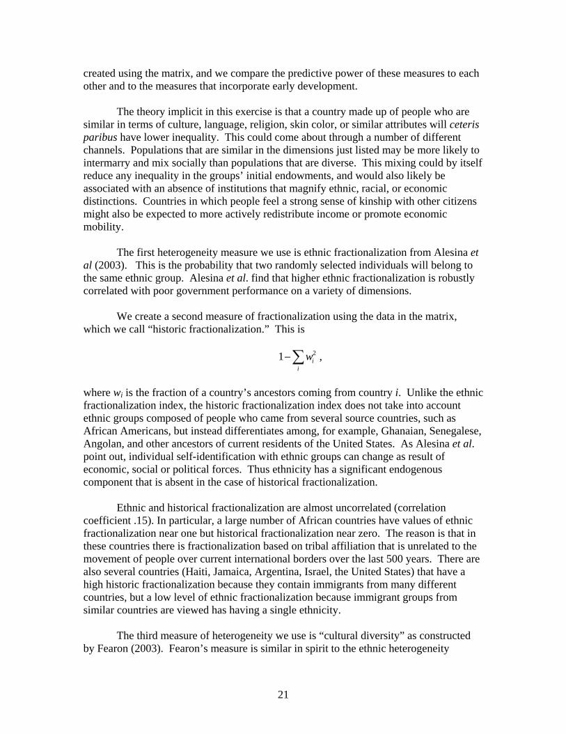
We create a second measure of fractionalization using the data in the matrix, which we call “historic fractionalization.” This is

21 i

iw−∑ ,

where wi is the fraction of a country’s ancestors coming from country i. Unlike the ethnic fractionalization index, the historic fractionalization index does not take into account ethnic groups composed of people who came from several source countries, such as African Americans, but instead differentiates among, for example, Ghanaian, Senegalese, Angolan, and other ancestors of current residents of the United States. As Alesina et al. point out, individual self-identification with ethnic groups can change as result of economic, social or political forces. Thus ethnicity has a significant endogenous component that is absent in the case of historical fractionalization.

Ethnic and historical fractionalization are almost uncorrelated (correlation coefficient .15). In particular, a large number of African countries have values of ethnic fractionalization near one but historical fractionalization near zero. The reason is that in these countries there is fractionalization based on tribal affiliation that is unrelated to the movement of people over current international borders over the last 500 years. There are also several countries (Haiti, Jamaica, Argentina, Israel, the United States) that have a high historic fractionalization because they contain immigrants from many different countries, but a low level of ethnic fractionalization because immigrant groups from similar countries are viewed has having a single ethnicity. The third measure of heterogeneity we use is “cultural diversity” as constructed by Fearon (2003). Fearon’s measure is similar in spirit to the ethnic heterogeneity

22

measure described above, but goes further in making an additional adjustment for different degrees of dissimilarity (as measured by linguistic distance) among the ethnic groups in a country’s population. Desmet, Ortuño-Ortín, and Weber (2009), using a similar measure, find that higher linguistic heterogeneity predicts a lower degree of government income redistribution. Our final measure of heterogeneity is similar in approach to Fearon’s, but instead of using the language that a country’s residents speak today, we use data on the languages spoken in the countries inhabited by their ancestors in 1500, according to our matrix. Differences in language may directly impede mixing of people from different source countries. In addition, linguistic closeness may well be proxying for other dimensions of culture (such as religion) that could have similar impacts on the degree of mixing among a country’s constituent populations and/or the openness of institutions.25 For these reasons, historical diversity in languages of a country’s ancestors may have an impact on inequality that lasts long after the residents of a country have come to speak the same language. We call the variable we create historical linguistic fractionalization (Our methodology and data are described in Appendix C). Table 10 presents regressions of income inequality, as measured by the gini coefficient, on our various measures of heterogeneity. The first four columns compare the four measures of heterogeneity described above. Cultural (linguistic) diversity is statistically insignificant. By contrast, the two variables that use the matrix to measure historical heterogeneity, historical fractionalization and historical linguistic fractionalization, as well as ethnic fractionalization enter very significantly with the expected positive sign. It is notable that in each case the measure of diversity based on historic variation performs better than the corresponding measure based on the current variation. For example, distance among the languages spoken by people’s ancestors predicts inequalities today far better than does distance among the languages spoken by those people themselves. In the case of variation in language, much of the superior predictive power is driven by Latin America which in terms of language currently spoken does not look very heterogeneous, but does look heterogeneous in terms of historic languages. Patterns of social differentiation which arose during the encounters of people from different continents appear to show persistence even after extensive intermixing and linguistic homogenization. Part of the reason for this could be that linguistic distance between ancestral populations posed barriers to transmission of technologies within countries of a similar kind to those which Spolaore and Wacziarg (2009) posit for genetic distance in international diffusion of technology. The next four columns of Table 10 repeat these regressions, controlling for the mean and standard deviation of the state history measures, as in columns 1 and 2 of Table

25 Spolaore and Wacziarg (2009) use genetic distance, a measure of the time since two populations shared a common ancestor, as an indicator of cultural similarity between countries. They argue that genetic distance determines the ability of countries to learn from each other, and show that it predicts income gaps among pairs of countries. Ethnic distance and genetic distance are closely related in practice, as shown by Cavalli-Sforza and Cavalli-Sforza (1995).

23

9.26 The somewhat surprising finding here is that variation in terms of state history dominates the other forms of heterogeneity that we examine. None of the other four measures of heterogeneity is statistically significant. Variation in early development among a country’s people is far more important than more standard forms of heterogeneity (in language or ethnicity) as an explanation for inequality. Similarly, variation in the linguistic background of a country’s ancestors, despite its surprising predictive power relative to that of present languages spoken, is not important once one controls for variation in early development. 3.3 Source Country Early Development as a Determinant of Relative Income The results in Tables 9 and 10 show that heterogeneity in the historical background of a country’s residents is correlated with income inequality today. A number of mechanisms could produce such a correlation. One simple theory is that when people with high and low statehist are mixed together, the high statehist people have some advantage which leads them to percolate up to the top of the income distribution, and then there is enough persistence that their descendants are still there hundreds of years later. A second theory is that situations in which high and low statehist people are mixed together tended to occur in cases of colonialization and/or slavery, and that in these circumstances high statehist people were able to create institutions that led groups at the top of the income distribution to remain there. We do not propose to test these theories against each other. Instead we test an auxiliary prediction that follows from either of them: specifically, in countries with a high standard deviation of statehist, it is the ethnic groups that come from high statehist countries that tend to be at the top of the income distribution. Confirming this prediction would give us additional confidence that the link between the standard deviations of statehist and the current level of inequality is not spurious. To test this prediction, we looked for accounts of socio-economic heterogeneity by country or region of ancestral origin in the ten countries in our sample having the highest standard deviation of statehist. It is in countries where statehist is highly variable where we would be most likely to find differences in outcomes among nationality groups with different values of statehist. The countries are listed in Table 11. Not surprisingly, all are former colonies, seven of them in the Americas. Of the latter, three are in Central America, three in South America, and one in the Caribbean. We also list in Table 11 the United States, which has the 17th highest standard deviation of statehist in the sample, and is of particular interest due to its size, economic importance, and good data availability. For each country in the table we first show the breakdown of the population in terms of origin countries or groups of similar countries, according to the matrix. We then

26 To save space, we don’t report parallel exercises using the standard deviation of agyears. In Section 3.3, we also focus on statehist. Tables 2, 3, and 4 show that statehist and agyears have similar explanatory power, and we accord slight priority to statehist because of its more nuanced tracking of 1500 years of social history (see our discussion comparing the two measures in Section 2).

24

show the weighted average value of statehist for each origin country or group. The next three columns are based on information about the current ethnic breakdown in the country. Ethnic groups as currently identified sometimes correspond to individual origin groups, but are often combinations, frequently labeled mestizos, mulatto, or creole. For each current ethnic group, we then present estimates of average statehist and the relative value of current income, listed as high, middle and low or high, upper middle, lower middle, and low. To estimate statehist for a mixed ethnic group we use the assumptions underlying the matrix that relate mixed groups to source populations. For example, the group termed “colored” in South Africa is assumed to have half of its ancestors coming in equal proportions from five European countries (England, Portugal, and Afrikaner source countries Netherlands, France and Germany) and the other half in unequal proportions from South Africa itself (35%), India (10%) and Indonesia (5%). These assumptions are reported in the region appendices describing the construction of the matrix.

Leaving details to Appendix D, we note immediately that the ordering of statehist values and the ordering of socio-economic status in Table 11 has at least some correspondence in every country. For nine of the eleven countries listed—Fiji, Cape Verde, Guyana, Paraguay, Panama, South Africa, Brazil, El Salvador and Nicaragua —the socio-economic ordering perfectly dovetails with that of statehist values. In two countries—Trinidad and Tobago and the United States—there are discrepancies in the orderings of Asians and “Whites,” with Chinese and (S. Asian) Indians having lower incomes than Whites in the first country despite having higher statehist, while Asians in general have higher incomes than Whites in the U.S. despite lower average statehist. For the U.S., there is a further discrepancy in that “Black” Americans have lower average incomes than American Indians and Alaska Natives, despite having somewhat higher average statehist values. While no statistical significance should be attached to the counts just mentioned, since the categorizations are quite broad and require some judgments to be made, the general pattern clearly supports the expectation.

A few patterns are noteworthy. Paraguay and El Salvador are representative of

the many Latin American countries in which the main identifiable groupings, listed in order of both socio-economic status and of average statehist, are European, mestizo, and Amerindian. Three of the represented countries— Panama, Nicaragua and Brazil—add a group of largely African descent to this tri-partite pattern. In each of the latter countries, the White group remains on top and the Amerindian group on the bottom. The Black group, with higher statehist than the Amerindians,27 is variously found on approximate par with the mestizos (Nicaragua) or between the mestizo and Amerindian groups (Panama). In fact in Brazil, mestizos, Blacks, and Amerindians are classified as low since data that discriminates more carefully between them is unavailable.

In two of the other represented countries of the Americas—Guyana and Trinidad

and Tobago—there are substantial populations of South Asian origin. In Trinidad and

27 This is due to the existence of some states in Africa before 1500 but their absence in the Americas outside of Mexico, Guatemala and the Andes. Note that the situation is reversed in some cases, for instance the indigenous people of South Africa have a lower statehist value than do those of Mexico and Peru.

25

Tobago, the socio-economic positioning of this group is lower than predicted by their average statehist. This result, contradicting our general hypothesis, may be related to the economic hard times on which South Asia itself had fallen by the 19th Century (mentioned in Section 2.4) and the manner in which millions were brought from that region to the Caribbean to work in indentured servitude after Britain outlawed slavery. Consistent with the expectations based on their homelands’ state histories, however, people of South Asian ancestry occupy middle or upper-middle socio-economic positions in Guyana and also in two of the three non-Americas examples, South Africa and Fiji.

Of the two African countries represented in Table 11, Cape Verde began as a

Portuguese plantation economy employing slaves brought from the African mainland. At the time of the country’s independence from Portugal, in 1975, the society was described as being stratified along color lines, with people of darker complexion usually found in the lower class and people of lighter complexion constituting the “bourgeoisie” (Meintel, 1984; Lobban, 1995). The correlation between complexion and socioeconomic class is consistent with our proposed explanation of the correlation between standard deviation of statehist and the gini coefficient seen in Tables 9 and 10. In South Africa, the major population categories are Black African, White, “colored” (with both European and either African, Indian, or Malay ancestors), and Indian or Asian. The socio-economic standings of these groups today remain heavily influenced by the history of European settlement and subordination of the local population, and partly as a result, the average incomes for those in the four groupings are ordered exactly in accord with the ordering of average statehist.

The only case in Table 11 not located in the Americas or Africa is Fiji, whose

population is classified by government statisticians as indigenous (55.0%), Indian (41.0%) and other (mainly European and Chinese, 4.0%). Average household incomes per adult in the three groups are ordered identically to average statehist values. Although the reported income gap between the Indian and native Fijian populations is far smaller than the difference in statehist, the government statisticians comment that the incomes of Indo-Fijians are probably undercounted, since much of it comes from private business activities likely to be underreported.

Turning finally to the U.S., the Census Bureau reports a breakdown of the population into White non-Hispanic, Hispanic any race, Black, Asian, American Indian and Alaska Native, and other small categories. These groups’ reported median incomes have the same ordering as their average statehist values, with the exception of the higher Asian than White income and the higher American Indian than Black income. The simple correlation between the five statehist and the five income values (as reported in Appendix D), with equal weighting on all observations, is 0.741. On balance, the evidence from the ten countries with the highest internal variation of statehist and from the seventeenth-ranking United States appears to support the idea that correlation between within-country differences in income and corresponding differences in the early development indicator statehist at least partially account for the predictive power of the standard deviation of statehist in the Table 9 and 10 regressions.

26

Indeed, in this section we have found within countries (as the previous section found between countries) that there is considerable persistence and reproduction of income differences which appears to reflect social differences dating back up to half a millennium. To be sure, in the majority of cases just discussed differences in societal capabilities during the era of European expansion played themselves out to a considerable degree in the form of outright dominance of some over others, including appropriation of land, control of government and monopoly of armed force, and involuntary movement of millions of people between macro-regions to meet the conquering population’s labor demands. How persistent early differences would have proven to be in the absence of the exercise of raw power is a question that goes beyond the scope of our paper. The point for present purposes is that as history has in fact unfolded, such differences have been remarkably persistent. 4. Conclusion

Conquest, colonialism, migration, slavery, and epidemic disease reshaped the world that existed before the era of European expansion. Over the last 500 years, there have been dramatic movements of people, institutions, cultures, and languages among the world’s major regions. These movements clearly have implications for the course of economic development. Existing literature has already made a good start at examining how institutions were transferred between regions and the long lasting economic effects of these transfers. However the human side of the story – the relationship between where the ancestors of a country’s current population lived and current outcomes – has received relatively little attention, in part due to the absence of suitable data. In this paper, we introduce a “world migration matrix” to account for international movements of people since the year 1500. We use the matrix to document some major features of world migration history such as the bi-modality of the distribution of indigenous and non-indigenous people by country and the variations in the primary source regions for immigrant-populated countries.

In the second part of the paper, we demonstrate the utility of the migration data by using it to re-visit the hypothesis that early development of agrarian societies and their sociopolitical correlates—states—conferred developmental advantages that remain relevant today. We confirm that in a global sample, countries on whose territories agriculture and states developed earlier have higher incomes. But we conjecture that people who moved from one region to another carried the human capabilities built up in that area with them. We find that re-calculating state history and agriculture measures for each country as weighted averages by place of origin of their people’s ancestors considerably improves the fit of these regressions. We also find that heterogeneity of early development, holding the mean level constant, is associated with higher per capita income. We interpret this finding as indicating that the effect of spillovers of growth-promoting characteristics between groups having different early development histories more than compensated for any negative effect on growth of higher inequality due to heterogeneity.

27

In Part 3, we show that the heterogeneity of a country’s population in terms of the

early development of its ancestors as of 1500 is strongly correlated with income inequality. We also show that heterogeneity with respect to country of ancestry or with respect to the ancestral language does a better job than does current linguistic or ethnic heterogeneity in predicting income inequalities today. As an additional test of the theory that early development conferred lasting advantage, we show that the rankings of ethnic or racial groups within a country’s income distribution are strongly correlated with the average levels of groups’ early development indicators.

The overall finding of our paper is that the origins of a country’s population – more specifically, where the ancestors of the current population lived some 500 years ago – matters for economic outcomes today. Having ancestors who lived in places with early agricultural and political development is good for income today, both at the level of country averages and in terms of an individual’s position within a country’s income distribution. Exactly why the origins of the current population matter is a question on which we can only speculate at this point. People who moved across borders brought with them human capital, cultures, genes, institutions, and languages. People who came from areas which developed early evidently brought with them versions of one or more of these things that were conducive to higher income. Future research will have to sort out which ones were the most significant. The fact that early development explains an ethnic group’s position within a country’s income distribution suggests that “good institutions” coming from regions of early development cannot be the whole story, although it does not prove that institutions are not of enormous importance. More research is also needed to understand how early development led to the creation of growth promoting characteristics (whatever these turn out to be), how these characteristics were transmitted so persistently over the centuries, as well as the process by which these characteristics are transferred between populations of high and low early development. Our hope is that the availability of a compilation of data on the reconfiguration of country populations since 1500 will make it easier to address such issues in future research.

28

References Acemoglu, D., Johnson, S., Robinson, J. (2001). “The colonial origins of comparative development: An empirical investigation,” American Economic Review 91 (5), 1369–1401. Acemoglu, D., Johnson, S., Robinson, J. (2002). “Reversal of fortunes: Geography and institutions in the makingof the modern world income distribution,” Quarterly Journal of Economics 117 (4), 1231–1294. Alesina, Alberto, Arnaud Devleeschauwer , William Easterly, Sergio Kurlat, and Romain Wacziarg, 2003. " Fractionalization," Journal of Economic Growth, vol. 8(2), pages 155-94, June. Ashraf, Quamrul, and Oded, Galor, “Human Genetic Diversity and Comparative Economic Development,” Working Paper, Brown University, 2008. Barro, Robert J., 2008, “Inequality and Growth Revisited,” Asian Development Bank Working Paper Series on Regional Economic Integration no. 11, January. Bockstette, Valerie, Areendam Chanda and Louis Putterman (2002). “States and Markets: The Advantage of an Early Start,” Journal of Economic Growth 7: 347-69. Burkett, John P., Catherine Humblet and Louis Putterman (1999). “Pre-Industrial and Post-War Economic Development: Is There a Link?” Economic Development and Cultural Change, 47 (3): 471-95. Cavalli-Sforza, Luigi L., and Frencesco Cavalli-Sforza (1995), The Great Human Diasporas. Reading, MA: Addison Wesley Publishing Co. Chanda, Areendam and Louis Putterman, 2006, “State Effectiveness, Economic Growth, and the Age of States,” pp. 69-91 in Matthew Lange and Dietrich Rueschemeyer, eds., States and Development: Historical Antecedents of Stagnation and Advance Basingstoke, England, Palgrave MacMillan, 2005. Chanda, Areendam and Louis Putterman (2007). “Early Starts, Reversals and Catch-up in the Process of Economic Development,” Scandinavian Journal of Economics 109, 387-413. Comin, Diego, William Easterly, and Erick Gong, “Was the Wealth of Nations determined in 1000 BC?” NBER Working Paper No. W12657, 2006. Comin, Diego, William Easterly, and Erick Gong, “Was the Wealth of Nations determined in 1000 BC?” Working paper, May 2009.

29

Correlates of War Project. (2000) Direct Contiguity Data, 1816-2000. Version 3.0. Online: http://correlatesofwar.org. Deininger, Klaus, and Lyn Squire, “A New Data Set and Measure of Income Inequality,” World Bank Economic Review, 10 (September) 1996, 565-591. Desmet, Klaus, Ignacio Ortuño-Ortín, and Shlomo Weber, “Linguistic Diversity and Redistribution,” Journal of the European Economic Association, 7:9, December 2009. Diamond, Jared, 1997, Guns, Germs and Steel. New York: W. W. Norton and Co. Easterly, William, “Inequality Does Cause Underdevelopment: Insights from a New Instrument,” Journal of Development Economics, Volume 84, Issue 2, November 2007, Pages 755-776. Engerman, Stanley, and Kenneth Sokoloff, “Factor Endowments, Inequality, and Paths of Development among New World Economies,” Economia 3.1 (2002) 41-109. Fearon, James, D., “Ethnic Structure and Cultural Diversity by Country,” Journal of Economic Growth, 8:2, June 2003, 195-222. Galor, Oded, and Omer Moav, “The Neolithic Origins of Contemporary Variation in Life Expectancy,” Mimeo, November 2007. Glaeser, Edward L., Rafael La Porta, Florencio Lopez-de-Silanes, and Andrei Shleifer, “Do Institutions Cause Growth?” Journal of Economic Growth, 2004, v9(3,Sep), 271-303. Hall, R., and C. Jones, (1999). “Why do some countries produce so much more output than others?” Quarterly Journal of Economics 114 (1), 83–116. Hibbs, Douglas A., and Ola Olsson, 2004, “Geography, biogeography, and why some countries are rich and others are poor,” Proceedings of the National Academy of Sciences 101: 3715-3720. Johnson, Allen and Timothy Earl, 1987, The Evolution of Human Societies: From Foraging Groups to Agrarian State. Stanford, CA: Stanford University Press. La Porta, Rafael, Florencio Lopez-de-Silanes, Andrei Shleifer, and Robert Vishny (1998). “Law and Finance,” Journal of Political Economy 106(6), 1113-1155. MacNeish, Richard (1991). The Origins of Agriculture and Settled Life. Norman, OK: University of Oklahoma Press. McEvedy, C. and R. Jones (1978). Atlas of World Population History, Viking Press.

30

Olsson, Ola, and Douglas A. Hibbs Jr., (2005). “Biogeography and Long-Run Economic Development,” European Economic Review, 49: 909-938. Putterman, Louis (2004). “State Antiquity Index Version 3”, available at http://www.econ.brown.edu/fac/Louis_Putterman/. Putterman, Louis, with Cary Anne Trainor (2006). “Agricultural Transition Year Country Data Set”, available at http://www.econ.brown.edu/fac/Louis_Putterman. Smith, Bruce (1995). The Emergence of Agriculture. New York: Scientific American Library. Sokoloff, Kenneth and Stanley Engermann (2000). “Institutions, Factor Endowments and Paths to Development in the New World,” Journal of Economic Perspectives 14: 217-232. Spolaore, Enrico, and Romain Wacziarg, 2009, “The Diffusion of Development” Quarterly Journal of Economics 124(2), May 2009, 469-527.

31

Table 1. Current population and descendants, by region.

Region

Population 1500 (millions)

Population 2000 (millions)

Population Growth Factor

Descendants per person of 1500

Fraction of current population descended from region’s 1500 ancestors

Fraction of descendants of 1500 population that live in same region

Number of descendants living outside the region (millions)

U.S. and Canada 1.12 315 281 9.14 .0325 1.00 0.00Mexico and Central America 5.80 137 23.6 16.8 .602 .846

15.0

The Caribbean 0.186 34.4 185 17.8 .0367 .381 2.05South America 7.65 349 45.6 10.5 .227 .988 0.927Europe 77.7 680 8.76 16.0 .975 .535 578North Africa/West and Central Asia 35.5 530 14.9 14.6 .939 .958

22.0

South Asia 103 1,320 12.8 12.9 .999 .990 13.2East Asia 132 1,490 11.3 11.6 1.00 .976 36.7Southeast Asia 18.7 555 29.7 28.5 .946 .988 6.50Australia and New Zealand 0.200 22.9 114 3.68 .0322 1.00 0.00Sub Saharan Africa 38.3 656 17.1 19.5 .981 .862 103

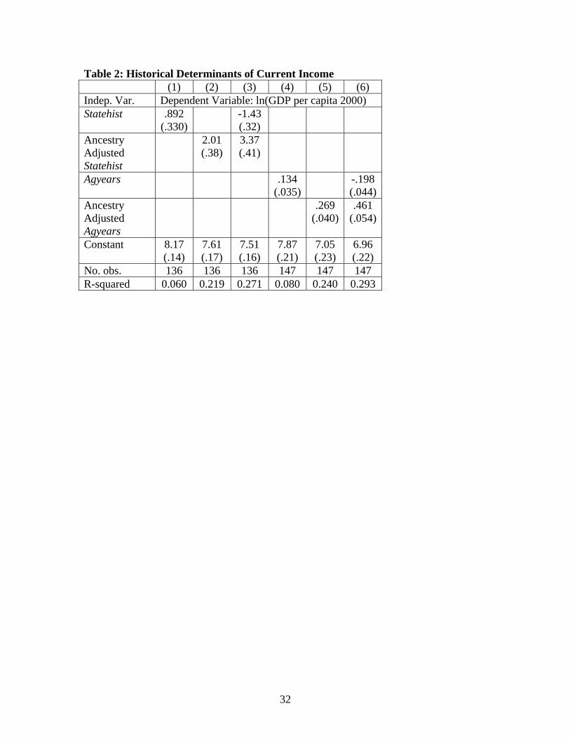
32

Table 2: Historical Determinants of Current Income (1) (2) (3) (4) (5) (6) Indep. Var. Dependent Variable: ln(GDP per capita 2000) Statehist .892

(.330) -1.43

(.32)

Ancestry Adjusted Statehist

2.01 (.38)

3.37 (.41)

Agyears .134 (.035)

-.198 (.044)

Ancestry Adjusted Agyears

.269 (.040)

.461 (.054)

Constant 8.17 (.14)

7.61 (.17)

7.51 (.16)

7.87 (.21)

7.05 (.23)

6.96 (.22)

No. obs. 136 136 136 147 147 147 R-squared 0.060 0.219 0.271 0.080 0.240 0.293

33

Table 3: Robustness to Alternative Measures of Migration, Descent, and Language (1) (2) (3) (4) (5) (6) (7) (8) (9) (10) (11) (12) Indep. Var. Dependent Variable: ln(GDP per capita 2000) Ancestry Adjusted Statehist

2.76 (.46)

2.09 (.38)

1.48 (.32)

2.11 (.38)

Ancestry Adjusted Agyears

.400 (.050)

.270 (.041)

.152 (.035)

.256 (.043)

“neo Europes” adjusted Statehist

1.27 (.32)

-.741 (.355)

“neo Europes” adjusted Agyears

.173 (.034)

-.133 (.040)

Native -.867 (.265)

-.744 (.270)

Retained -.800 (.361)

-.583 (.358)

Fraction European Descent

1.82 (.16)

1.63 (.16)

1.58 (.17)

Fraction European Languages

1.31 (.21)

1.04 (.18)

1.06 (.19)

Constant 8.02 (.14)

7.55 (.17)

7.66 (.19)

7.00 (.22)

8.87 (.44)

8.07 (.43)

7.83 (.10)

7.27 (.13)

7.11 (.19)

8.10 (.14)

7.26 (.17)

6.86 (.23)

No. obs. 136 136 147 147 129 139 138 138 138 113 113 113 R-squared 0.122 0.230 0.127 0.259 0.286 0.281 0.458 0.572 0.526 0.195 0.418 0.393

34

Table 4: Historical and Geographical Determinants of Current Income Panel A (1) (2) (3) (4) (5) (6) Indep. Var. Dependent Variable: ln(GDP per capita 2000) Ancestry Adjusted Statehist

2.38 1.32 2.21 1.75 1.31 1.24 (0.40) (0.43) (0.41) (0.55) (0.42) (0.42)

Absolute Latitude

0.0386 0.0337 (0.0062) (0.0084)

Landlocked -0.628 -0.558 (0.272) (0.172) Eurasia 0.594 -0.327 (0.286) (0.247) Climate 0.609 0.235 (0.096) (0.121) Constant 7.44 6.94 7.65 7.44 6.92 6.99 (0.17) (0.15) (0.21) (0.16) (0.17) (0.20) No. Obs. 111 111 111 111 111 111 R-squared 0.294 0.527 0.339 0.334 0.494 0.593

Panel B (1) (2) (3) (4) (5) (6) Indep. Var. Dependent Variable: ln(GDP per capita 2000) Ancestry Adjusted Agyears

0.313 0.172 0.289 0.219 0.178 0.153 (0.048) (0.053) (0.051) (0.062) (0.060) (0.054)

Absolute Latitude

0.0393 0.0404 (0.0058) (0.0087)

Landlocked -0.500 -0.577 (0.236) (0.160) Eurasia 0.631 -0.172

(0.250) (0.237) Climate 0.516 0.053 (0.101) (0.133) Constant 6.85 6.61 7.07 7.04 6.74 6.80 (0.25) (0.21) (0.28) (0.26) (0.25) (0.25) No. Obs. 116 116 116 116 116 116 R-squared 0.293 0.523 0.320 0.334 0.426 0.563

35

Table 5: Alternative Measures of Early Historical Development (1) (2) (3) (4) (5) (6) (7) (8) Indep. Var. Dependent Variable: ln(GDP per capita 2000) Geo Conditions 0.752

(0.075) Ancestry Adjusted Geo Conditions

0.952 (0.069)

Bio Conditions 0.746 (0.081)

Ancestry Adjusted Bio Conditions

0.947 (0.074)

Technology Index 1 CE

0.0924 (0.3758)

Ancestry Adjusted Technology Index 1 CE

2.51 (0.59)

Technology Index 1500 CE

1.55 (0.30)

Ancestry Adjusted Technology Index 1500 CE

3.26 (0.30)

Constant 8.42 8.19 8.43 8.21 8.42 6.41 7.77 6.54 (0.09) (0.08) (0.09) (0.07) (0.28) (0.46) (0.20) (0.21)

Observations 105 105 105 105 125 125 114 114 R-squared 0.415 0.574 0.417 0.581 0.000 0.133 0.183 0.525

36

Table 6: Historical Determinants of Current Institutions (1) (2) (3) (4) (5) (6) Indep. Var. Executive

Constraints Expropriation Risk Government

Effectiveness Statehist 0.158 0.658 0.445

(0.274) (0.287) (0.271) Ancestry Adjusted Statehist

0.670 1.33 1.32 (0.309) (0.33) (0.30)

Constant 1.95 1.71 3.89 3.51 -0.180 -0.604 (0.13) (0.15) (0.13) (0.15) (0.114) (0.118)

No. obs. 141 141 111 111 144 144 R-squared 0.002 0.033 0.047 0.134 0.019 0.123 Note: All dependent variables are normalized to have a standard deviation of one.

37

Table 7: Source Regions and Current Regions as Determinants of Current Income Regression number

(1) (2) (3)

Independent Variables

Source Regions

Current Regions

Source Regions

Current Regions

U.S. and Canada 33.7 (5.6)

3.03 (0.16)

-2,273 (384)

74.8 (12.4)

Mexico and Central America

0.380 (0.495)

1.10 (0.24)

1.90 (1.25)

-0.870 (0.710)

The Caribbean 3.67

(0.81) 1.33

(0.30) 0.834

(1.884) 0.268

(0.221)

South America 0.498

(0.229) 1.35

(0.20) 1.11

(0.51) -0.415

(0.419)

Europe 2.35

(0.16) 2.23

(0.18) 2.66

(0.47) -0.265 (0.476)

North Africa/West and Central Asia

1.29 (0.21)

1.28 (0.21)

0.654 (1.349)

0.613 (1.248)

South Asia 0.872

(0.265) 0.388

(0.175) 3.05

(0.39) -2.53 (0.39)

East Asia 2.15

(0.54) 1.81

(0.56) 4.77

(0.57) -2.81 (0.87)

Southeast Asia 0.805

(0.242) 1.07

(0.32) 1.59

(0.63) -0.913 (0.500)

Australia and New Zealand

8.09 (2.10)

2.72 (0.17)

-1.59 (0.87)

0.436 (0.444)

Constant 7.27 (0.11)

7.34 (0.13)

7.22 (0.12)

No. obs. 152 152 152 R-squared 0.631 0.584 0.681 Note: In regression 1, the independent variables are the shares of the population in each country originating in each region. In regression 2, the independent variables are dummies for a country being located in a particular region. In regression 3 the independent variables are both of the above.

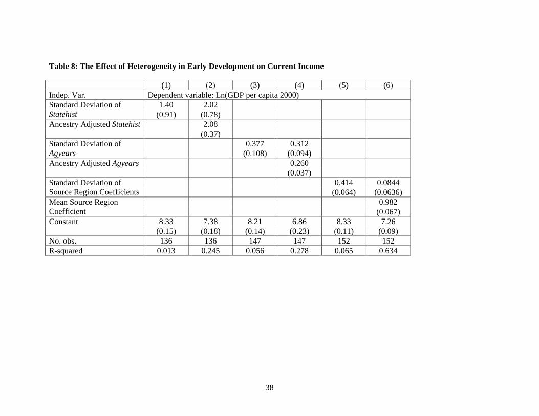
38

Table 8: The Effect of Heterogeneity in Early Development on Current Income (1) (2) (3) (4) (5) (6) Indep. Var. Dependent variable: Ln(GDP per capita 2000) Standard Deviation of Statehist

1.40 2.02 (0.91) (0.78)

Ancestry Adjusted Statehist 2.08 (0.37)

Standard Deviation of Agyears

0.377 0.312 (0.108) (0.094)

Ancestry Adjusted Agyears 0.260 (0.037)

Standard Deviation of Source Region Coefficients

0.414 0.0844 (0.064) (0.0636)

Mean Source Region Coefficient

0.982 (0.067)

Constant 8.33 7.38 8.21 6.86 8.33 7.26 (0.15) (0.18) (0.14) (0.23) (0.11) (0.09)

No. obs. 136 136 147 147 152 152 R-squared 0.013 0.245 0.056 0.278 0.065 0.634

39

Table 9: Historical Determinants of Current Inequality (1) (2) (3) (4) (5) (6) Indep. Var. Dependent variable: Gini Coefficient Standard Deviation of statehist

0.456 0.408 (0.088) (0.084)

Ancestry Adjusted statehist

-0.148 (0.036)

Standard Deviation of agyears

0.0512 0.0571 (0.0121) (0.0108)

Ancestry Adjusted agyears

-0.0217 (0.0052)

Standard Deviation of Source Region Coefficients

0.0207 0.0453

(0.0166) (0.0153)

Mean Source Region Coefficient

-0.0743 (0.0089)

Constant 0.375 0.445 0.381 0.493 0.413 0.498 (0.014) (0.024) (0.014) (0.031) (0.011) (0.016)

No. obs. 135 135 140 140 141 141 R-squared 0.140 0.267 0.108 0.260 0.018 0.365

40

Table 10: Ethnic, Linguistic, and Historical Determinants of Current Inequality (1) (2) (3) (4) (5) (6) (7) (8) Indep. Var. Dependent variable: Gini Coefficient from WIID2 Ethnic Fractionalization

0.117 0.0517 (0.037) (0.0355)

Historical Fractionalization

0.134 -0.0116 (0.034) (0.0489)

Cultural Diversity 0.0354 0.0126 (0.0437) (0.0382)

Historical Linguistic Fractionalization

0.168 0.0460 (0.039) (0.0721)

Standard Deviation of Statehist

0.392 0.435 0.401 0.310 (0.085) (0.124) (0.086) (0.167)

Ancestry Adjusted Statehist

-0.130 -0.148 -0.151 -0.149 (0.040) (0.037) (0.038) (0.036)

Constant 0.367 0.382 0.407 0.385 0.415 0.446 0.441 0.445 (0.019) (0.014) (0.017) (0.013) (0.033) (0.025) (0.030) (0.024)

No. obs. 132 135 132 135 132 135 132 135 R-squared 0.073 0.101 0.005 0.115 0.276 0.267 0.275 0.269

41

Table 11: Statehist and relative income for ancestry groups and current ethnic groups

# Country Standard Dev. of Statehist

Gini28 Component groups (region)

Percent population29

Statehist (average)

Component groups (ethnic)

Percent population30

Statehist (average)

Relative Income

1 Fiji .346 .441 European 2.2 0.693 Other31 4 0.745 High Indian 45.0 0.688 Indo-Fijian 41 0.688 Middle Fijian 52.1 0.000 Fijian 55 0.000 Low

2 Cape Verde

.301 .51 Portuguese 41.4 0.723 White 1.0 0.723 High African 58.6 0.142 Creole 71.0 0.473 Middle Black 28.0 0.142 Low

3 Guyana .293 .540 Chinese 0.7 0.906 Chinese 0.3 0.906 High Portuguese 1.3 0.723 Portuguese 0.4 0.723 Middle Mixed32 11.2 0.410 Middle S. Asian 54.0 0.677 East-Indian 51.9 0.677 Middle African 39.0 0.142 Black 30.8 0.142 Middle Guyanese 5.0 0.000 Amerindian 5.3 0.000 Low

4 Panama .292 .548 Chinese 1.5 0.906 Chinese 2.0 0.906 High S. Asian 4.0 0.677 White 10.0 0.578 High European 45.2 0.578 Mestizo 68.0 0.281 Upper

Middle

28Source: UN World Income Inequality Database (2007), except: Cape Verde – World Development Indicators, 2001 29 Computed from Matrix. 30 Based on: Fiji – Household Survey 2002-03; Cape Verde – Census 1950 (quoted in Lobban, R., “Cape Verde: Crioulo Colony to Independent Nation”, 199); Guyana – Census 1980; Paraguay – Census 2002; Panama – Fearon, J. D. Data set described in "Ethnic and Cultural Diversity by Country". Journal of Economic Growth 8, 2 (June 2003): 195-222.; South Africa – Household Survey 2005; Trinidad and Tobago - Continuous Sample Survey of Population; El Salvador – CIA Factbook; Nicaragua – CIA Factbook; Venezuela – CIA Factbook,; United States - U.S. Census, Vintage 2004 31 Europeans, Chinese 32 ½ East Indian, ½ African

42

African 13.0 0.150 mixed West-Indian (Black)

13.0 0.150 Lower Middle

Panamanian 35.7 0.000 Amerindian 6.0 0.000 Low 5 Paraguay .291 .552 European,

non-Spanish5.5 0.749 European

(incl. Spanish)

3.8 0.575 High

Spanish 46.8 0.562 Mestizo 94.7 0.281 Middle Paraguayan / Brazilian

46.1 0.000 Amerindian 1.1 0.000 Low

6 South Africa

.289 .565 European 18.0 0.710 White 9.2 0.710 High Indian / S. Asian

3.4 0.670 Indian / Asian

2.5 0.670 Upper Middle

South-African

78.7 0.000 Colored (mixed)33

8.9 0.452 Lower Middle

Black African

79.4 0.000 Low

7 Brazil .288 .566 Japanese 0.8 0.834 Asian 0.4 0.834 High European 74.4 0.715 White 53.7 0.715 Middle Mixed34 38.5 0.384 Low African 15.7 0.086 Black 6.2 0.086 Low Brazilian 9.1 0.000 Amerindian 0.4 0.000 Low

8 Trinidad and Tobago

.284 .402 Chinese 1.5 0.906 Chinese 0.2 0.906 Upper Middle

European 7.1 0.671 White / Caucasian

0.7 0.671 High

S. Asian 45.4 0.677 Indian 40.5 0.677 Low

33 .35 African, .1 S. Asian, .05 Indonesian, .1 UK, .1 Netherlands, .1 France, .1 Germany and .1 Portugal 34 .506 European, .239 Amerindian, .255 African

43

African 46.0 0.166 Mixed35 14.9 0.504 Lower Middle

African 43.5 0.166 Low 9 El

Salvador .281 .484 Spanish 50.0 0.562 White 9.0 0.562 High

Salvadoran 50.0 0.000 Mestizo 90.0 0.281 Middle Amerindian 1.0 0.000 Low

10 Nicaragua .277 .544 European 51.0 0.568 White 17.0 0.568 High African 9.0 0.150 African

(Creole) 9.0 0.150 Middle

Nicaraguan 40.0 0.000 Mestizo 69.0 0.281 Middle Amerindian 5.0 0.000 Low

17 United States

.232 .464 European 75.7 0.648 White not Hispanic

67.4 0.650 Upper Middle

Asian 4.1 0.640 Asian 4.2 0.640 High Central and South American

6.3 0.433 Hispanic of any race

14.1 0.485 Lower Middle

Sub-Saharan African

9.6 0.146 Black 12.8 0.240 Low

North-American36

3.2 0.000 American Indian and Alaska Native

1.0 0.000 Lower Middle

35 1/3 African, 1/3 S. Asian, 1/3 European. 36 Includes Hawaii and Alaska

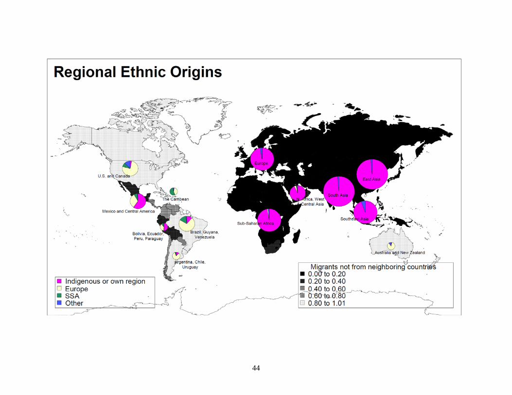
44

45

Figure 1a Distribution of countries by Figure 1b Distribution of world proportion of ancestors from own or population by proportion of immediate neighboring country. ancestors from own or immediate neighboring country.

46

47

48

Appendix A: World Migration Matrix, 1500 – 2000*

The goal of the matrix is to identify where the ancestors of the permanent residents of today’s countries were living in 1500 C.E. In this abbreviated description, we address some major conceptual issues relevant to the construction of the matrix and identify some of the main sources of information consulted. The migration matrix is a table in which both row and column headings are the names of presently existing countries, and cell entries are estimates of the proportion of the ancestors of those now permanently residing in the country identified in the row heading who lived in the country identified by the column heading in 1500. An ancestor is treated as having lived in what is now, say, Indonesia, if the place they resided in that year is within the borders of Indonesia today. When ancestors could be identified only as part of an ethnic group that lived in a region now straddling the borders of two or more present-day countries, we try to estimate the proportion of that group living in each country and then allocate ancestry accordingly. For example, if a given ancestor is known to have been a “Gypsy” (Roma) but if we have no information on which country he or she lived in during the year 1500, we apply an assumption (see Appendix B) regarding the proportion of Gypsies who lived in Greece, Romania, Turkey, etc., as of 1500. The Gypsy example is one of many illustrating the fact that most of our data sources organize their information around ethnic groups rather than territory of origin. While the use of information on ethnicity was unavoidable in the process of constructing the matrix, it was not a focus of attention in its own right. In cases in which ancestors are known to have migrated more than once between 1500 and 2000, countries of intervening residence are not indicated in the matrix. For example, an Israeli whose parents lived in Argentina but whose grandparents arrived in Argentina from Ukraine, is listed as having had ancestors in Ukraine. People of mixed ancestry are common in many countries, for example people of mixed Amerindian and Spanish ancestry in Mexico. Such individuals are treated as having a certain proportion of their ancestry deriving from each source country. When members of such groups are reported to account for 30% or more of a country’s population, we searched the specialized scientific literature on genetic admixture for the best available estimates. For smaller mixed groups we base estimates on the stated or implicit assumptions of conventional sources or on extrapolation from similar countries in which we had genetic estimates. Our

* This is an abbreviated version of Appendix B, which is linked to region summaries and the data set itself. All can be found at http://www.econ.brown.edu/fac/Louis_Putterman/ .

49

assumed breakdowns of mixed populations for each country are discussed in Appendix B. Because our interest is in the possible impact of its people’s origins on each country’s economic performance, we try to identify the origins of long-term residents only, thus leaving out guest or temporary workers. Very little data is available about the duration of stay of most temporary workers, so we made educated guesses as to what portion of the originally temporary residents have become permanent, understood as having been in the country at least ten years as of 2000. The matrix includes entries on all countries existing in 2000 having populations of one half million or larger. A country is included as a source country for ancestors of the people of another country if at least 0.5% of all ancestors alive in 1500 are estimated to have lived there. Some entries smaller than 0.5% are found in the matrix, but these occur as a result of special decompositions applied to populations that our sources identify by ethnic group rather than by country of origin—e.g. Gypsies, Africans (descended from slaves, especially in the Americas), and Ashkenazi Jews. Appendix B details the method of assigning fractions of these populations to individual source countries.

Some of the more important sources from which data were drawn for the construction of the matrix are listed below. See Appendix B and its regional sub appendices for other sources and details.

Columbia Encyclopedia (online edition) CIA World Factbook Countriesquest.com Encyclopædia Britannica (online edition) Everyculture.com Library of Congress, Federal Research Division, Country Studies MSN Encarta Encyclopedia (online edition) Nationsencyclopedia.com World Christian Database (Original source for WCE) World Christian Encyclopedia