Research Office A State Affiliate of the U.S. Census Bureau

Population Projections Methodology

March 2013

1

I. INTRODUCTION

The Population Projections for Ohio and Counties by Age and Sex: 2010 to 2040 are recognized as the State of Ohio projections to be used for planning and forecasting by state, county and local governments. The Projections are an extrapolation of past and current demographic trends into the future. The projections do not attempt to model policy initiatives. The projections are not intended to constrain or to advocate specific levels of growth at the county level. These projections should be viewed as a guide, as a starting point, for planning the future needs of Ohio residents. This monograph is an explanation of the methods and procedures employed in generating Ohio's population projections. The report includes the decisions made in data collection, projection method, as well as fertility, mortality, and migration assumptions. All input data -- base year population by age/sex, institutional population by age/sex, age-specific fertility rates by county, census survival rates by county, estimated and projected migration rates and age/sex proportion of migration by county -- were calculated and prepared using Microsoft Excel software. II. METHODOLOGICAL OVERVIEW Projection Model Populations of 2010-2040 for the State of Ohio and its 88 counties were projected using a demographic based cohort-component projection model. The basic logic of this model is that future population is a function of present (baseline) population plus the three components of demographic change: births, deaths, and migration. Computations are carried out individually to reflect variations in birth, death, and migration rates for each cohort. The base formula used in the projection model to express this function is: Populationt+5 = Populationt + t+5Birtht - t+5Deatht + t+5Net Migrationt

Where t = time, in years. The birth component is calculated by multiplying the base-year female population age 15-19 through 40-44 by the projected Age-Specific Fertility Rates (ASFRs), summing the six products (six female age groups), then multiplying by five (the period of the projection is five years). The result of this calculation is the number of births projected to occur over the projection period.

2

The death component is calculated by multiplying each age/sex specific baseline-year cohort population by the projected five-year survival rate. This calculation results in the number of survivors of that cohort to the projected year. The actual number of projected deaths can be calculated, then, as the difference between the base population minus the survived (or expected) population, although number of deaths do not enter directly into the calculation of projected population. The migration component is calculated for each county by multiplying the expected population by the appropriate projected county total net migration rate. The county total net migration rates are projected based on the historical (1970-2010) net migration rates, as well as the most recent (2000-2010) gross migration trend from Internal Revenue Service (IRS) migration data. Both migration data sets are available by county. The county age/sex-specific migrants are calculated by multiplying each county's 2000-2010 age/sex proportionate rates of migration by the appropriate projected county total net migration. Use of the following formulas are explained and documented in the following text. a. Projected Sex-Specific Population Aged 0-4 Years Old:

)1(**)5115.0*(ˆ0404

504

ttty MSBM

)1(**)4885.0*(ˆ0404

504

ttty MSBF

Where,

504

ˆ yM and 504

ˆ yF are the projected male and female populations 0-4 years old in

the projected year y+5; Bt is total births in the 5-year time interval t; 4S0

t is the survival rate for persons age 0-4 (by sex) in the 5-year time interval t;

4M0

t is the net migration rate for persons 0-4 years old (by sex) in the 5-year time interval t; 0.488 is the ratio of male-to-total births; and,

0.512 is the ratio of female-to-total births (birth ratios based on Ohio live births,

3

2000-2010). b. Projected Population Age 5-84 Years Old:

)1(**ˆ555

5

15t

it

iy

iy

i MSPP

Where,

5

15ˆ

yiP is the projected population of 5-year age interval i+1 (by sex), in the

projected year y+5; 5Pi

t is the population of 5-year age interval i (by sex), in year y;

5Sit is the survival rate for persons in the 5-year age interval i (by sex) for the 5-

year time interval t; 5Mi

t is the net migration rate for persons in the 5-year age interval i (by sex) for the 5-year time interval t. c. Projected Population Age 85 and Over: P85

y+5 = (5P80y + P85

y) *85S80t * (1 + M85

t) Where, P85

y+5 is the projected population age 85 and over (by sex) in the projected year y+5; 5P80

y and P85y are the total populations age 80-84 and 85 and over (by sex) in

year y; 85S80

t is the survival rate for age group 80 and over surviving to 85 and over in the 5-year time interval t (by sex); M85

t is the total net migration rate for persons age 85 and over (by sex) in the five-year time interval t. Appendix 1 shows a flow chart describing the population projection procedure in its entirety.

4

Deriving Base-Line Rates Several tests were done at the state level to determine which fertility and mortality rates should be used in this projection series. Projected 2000-2005 and 2005-2010 county births were forced to align with the 2000-2005 and 2005-2010 registered county births recorded with the Ohio Department of Health (Appendix 7). This was accomplished by adjusting the projected fertility rates until the projected births matched the registered births. The result showed that, for obtaining a better match between the projected and registered births, a linear extrapolation of the Age-Specific Fertility Rates (ASFRs) for 2000-2005 and 2005-2010 could be used to derive projected ASFRs and Total Fertility Rates (TFRs). Therefore, this linear method was used for most of the counties. However, for eleven counties, a percent adjustment was made to the linear extrapolations to get projected ASFRs and TFRs. Those eleven counties are: Clinton, Geauga, Paulding, Preble, Licking, Lawrence, Warren, Mercer*, Meigs*, Noble*, and Van Wert* counties. In the counties with “*”, the percent adjustment was used for only part of the age groups or part of the projected years. The state level projected ASFRs and TFRs were used for the counties of Athens, Franklin and Wood. Projected 2000-2005 and 2005-2010 county deaths were forced to align, respectively, with the 2000-2005 and 2005-2010 registered county deaths, recorded with the Ohio Department of Health (Appendix 8). The projected deaths were calculated by different survival rate methods, such as the census survival rate method and the life table survival rate method. By comparing the projected deaths with the registered deaths, the census survival rate method was chosen because of the better match. Projected 2005 and 2010 state populations were forced to align, respectively, with 2005 estimates and 2010 Census county population counts produced by the U.S. Bureau of the Census (see Appendix 9). This was accomplished by using different migration rates until the projections matched the state total estimate and census population counts. By comparing the projected population with the estimate and census population, a projected migration model which combined the historical migration rates and the last ten years’ (2000-2010) IRS migration trends was chosen because of the better match. Projecting future trends of these three components from the base year (2010) is an important aspect of the methodology. Assumptions concerning fertility, mortality and migration trends at both state and county levels are discussed separately in this report.

5

III. BASE AND INSTITUTIONAL POPULATIONS Base Population The base year for the population projections is 2010. Specifically, the base time is April 1, 2010 - the official day of the census enumeration. All projected figures stem from that date. Five-year age cohorts by sex, ranging from 0-4 years of age to 80-84 and 85+ at the county level were drawn from the 2010 Census of Population and Housing, Summary File 1 {Source: Census of Population and Housing, 2010: SF 1 (Ohio) [machine-readable data files] / prepared by the Census Bureau. Washington, D.C.: the Bureau [producer and distributor], 2011. Tables P12, P12A, P12B, PCT13, PCT13A & PCT13B}. Institutional Population The calculation of sub-state projections customarily requires special treatment of institutional populations such as universities, prisons and military installations. It is important to separate these institutional populations from the county residents, since their fertility and migration patterns are vastly different. These special populations usually are replaced periodically by other individuals of the same age group. For this reason, it is expected that the age and sex composition of these groups will remain approximately the same over the projected period. Not isolating the populations in these institutions would pose several problems:

1. If these individuals are “survived” – i.e., survival rates applied to them so as to age them to the subsequent age group, as they are to county residents, an inaccurate migration and cohort population would result in the next projected period for the subsequent age cohort;

2. Applying standard fertility rates to female university students would produce unrealistically high county birth figures, since births to students are relatively rare. To circumvent these potential errors, institutional populations of each county were extracted from the 2010 Census counts by age and sex. These populations subsequently were projected separately from the resident population. After calculating mortality, fertility and migration for the county resident population, the institutional populations were added into the county populations by age and sex for each projected period. The assumption was that these groups will remain consistent in age/sex structure composition, unlike the general population.

6

Projected Institutional Population The projection of institutional populations within a context of an aging population presented a problematic situation. Institutional populations, to a certain extent, reflect the age structure at that point in time. In 2000, the population most “at risk” of being a student, inmate, or member of the Armed Forces (18-24 years old) was disproportionately large, commonly known as the "baby boom" population. Over the projected time period, this population is replaced by a significantly smaller population. On the other hand, more recent population information indicates a higher or lower institutional participation rate of the population at risk. The state total institutional population has increased or decreased. To average both the influences of aging and the increasing institutionalization rate, two assumptions were made, as follows: 1. The projected institutional populations would remain at the 2010 proportionate rates of institutional population to county population, by age and sex, but would not remain at the 2010 proportionate numbers of institutional population to county population, by age and sex. These proportionate rates were applied to the county-level projected populations at each five-year time interval to derive county total institutional population by age and sex. This assumption will result in more projected institutional persons for older age groups than for younger age groups because of the aging of the population. 2. The increased or decreased of the institutional population will be decided by the change of the institutional population between 2000 and 2010 by each county for each five year period throughout the projection period. This assumption would allow for increasing/decreasing institutional populations in the future. The following is the formula to project and add the institutional population into the total population by age/sex: 5TPy+5

i = 5UGQy+5i + GQ2010 * xn * 5GQP000-10

i Where,

5TPy+5i is the projected total population for the year y+5 and the 5-year age group i,

where y can take a value from 2010 to 2035 and i can take a value from 0-4 to 80-84 age group;

5UGQy+5i is the projected population without institutional population for the year y+5

and the 5-year age group i; GQ2000 is the total institutional population for the year 2000; x is the rate of change in institutional population for each projection period; and n represents the number of the projection period, which can change from 1 to 6; 5GQP90-00

i is the proportion of institutional population for each age/sex group to the total for the time period 2000-2010.

7

IV. FERTILITY Fertility Assumptions Generally speaking, the fertility trend for Ohio from 2000 to 2010 increased slightly in total fertility rates (total fertility rate of 1,954 for 2000-2005 and 1,972 for 2005-2010). This slight increase is due to countervailing increases in fertility rates for the 25-29, 35-39 and 40-44 age groups, and declines in the fertility rates for the female age groups 15-19, 20-24 and 30-34 (See Table 1). As a result, Ohio's fertility rates were projected to increase slightly for the entire 2010 to 2040 projection time frame. Ohio's total fertility rate (births per thousand women age 15 to 49) is projected to increase from 1,981 (2010-2015) to 2,027 (2035-2040) (see Table 1).

TABLE 1

ESTIMATED & PROJECTED AGE-SPECIFIC FERTILITY RATES AND TOTAL FERTILITY RATES:

OHIO, 1980-1985 TO 2035-2040 ==================================================================== ESTIMATED ASFR PROJECTED ASFR --------------------------- ------------------------------------------------------------------------- AGE 00-05 05-10 10-15 15-20 20-25 25-30 30-35 35-4015-19 0.040 0.039 0.038 0.038 0.038 0.037 0.037 0.03620-24 0.107 0.103 0.101 0.098 0.096 0.094 0.092 0.08925-29 0.112 0.118 0.122 0.125 0.128 0.132 0.135 0.13930-34 0.090 0.089 0.089 0.088 0.088 0.087 0.087 0.08635-39 0.035 0.038 0.039 0.040 0.042 0.043 0.044 0.04640-44 0.007 0.007 0.008 0.008 0.008 0.009 0.009 0.009

TFR 1,954 1,972 1,981 1,990 1,999 2,009 2,018 2,027 ====================================================================

Data source: Ohio Development Services Agency, Office of Research (JH), P.O. Box 1001, Columbus, Ohio 43216-1001, March, 2013 The projected total number of Ohio births, however, will increase from 704,313 (2010-2015) to 731,079 (2035-2040) due, in large part, to the assumption that the relatively large female cohort comprised of the children of the “baby boomers” – commonly referred to as the “baby boomlet”-- will continue the recent trend of delaying childbearing until into their thirties. Table 2 below shows Ohio's five year total births and age-specific births over the projected years.

8

TABLE 2

PROJECTED FIVE-YEAR TOTAL & AGE-SPECIFIC BIRTHS:

OHIO, 2010-2015 to 2035-2040

AGE 10-15 15-20 20-25 25-30 30-35 35-40

15-19

71,133

68,608

65,796

66,254

66,472

67,271

20-24

177,317

178,981

169,495

164,256

167,530

164,218

25-29

217,905

220,797

232,156

231,933

237,505

251,893

30-34

152,760

156,497

154,234

156,799

151,435

151,224

35-39

70,351

69,014

73,628

75,429

79,624

79,846

40-44

14,846

14,398

14,193

15,231

15,691

16,628

TOTAL

704,313

708,294

709,503

709,902

718,257

731,079 Data source: Ohio Development Services Agency, Research Office (JH), P.O. Box 1001, Columbus, Ohio 43216-1001, March, 2013 Age-specific fertility rates (ASFR) are used in this series to project future birth rates and births. ASFRs are determined for each five-year female age group between 15-19 to 40-44, and are calculated by dividing the number of live births to women in the appropriate five-year age groups by the number of females within that age group. A linear extrapolation based on the ASFRs of 2000-2005 and 2005-2010 was used to produce projected ASFRs: Estimated ASFRs: x+5ASFRx

t = x+5Bxt / x+5Fx

t

Projected ASFRs: 5x+5ASFRx

t = 05x+5ASFRx

00 * [1 + (105ASFRx

05 - 055ASFRx

00) / 2 * n] Where, ASFR is the age-specific fertility rate; x and x+5 is a five-year female cohort beginning with initial age x, to x+5;

9

t is time in single years; x+5Bx

t is the average number of births to a stationary female five-year age cohort (e.g., average births [x+5Bx

t] to females 20-24 years old in the time period 2000-05 is the average of births to females 20-24 years old in 2001, 2002…2005); F is the female population within the five-year age cohort; 95

i+5ASFRx95 and 95

x+5ASFRx90 are single-year age-specific fertility rates for the

years 2005-2010 and 2000095 by county; n is the number of projection periods from 2010, 1 being 2015, 2 being 2020, etc.. The 2005-2010 ASFRs were used for the entire projection period for eleven counties: Clinton, Geauga, Paulding, Preble, Licking, Lawrence, Warren, Mercer*, Meigs*, Noble* and Van Wert*. The 2005-2010 ASFRs for were used for part of female age groups or part of the projected years for the last four counties with the “*”. The 2005-2010 ASFRs for these counties were so high that a decision was made not to allow them to increase further. The state level ASFRs were used for the counties of Athens, Franklin and Wood because the option to remove an unquantifiable number of 15 to 24 year-old females, in order to bring the ASFRs to reasonable values, may have been more problematic. Appendix 10 shows the estimated ASFRs and TFRs for the periods 2000-2005 and 2005-2010 by county. Total births for each five-year period can be projected based on the projected ASFRs and the female populations of each childbearing age group: t+5Bt = t+5

49 Ó 15t [(t+5

x+5ASFRxt * 5 * x+5Fi

y)] Where, t+5Bt is the total projected births for the five-year time interval t; t+5

49Ó15t is the sum of births for each female childbearing age group (15-19 to 45-

49) in the five-year time interval t; t+5

5ASFRxt is the single-year age-specific fertility rate for females age x to x+5 in

the projected five-year time interval t; and 5Fi

y is the female population within the five-year age cohort i in year y; multiplication by 5 translates single-year ASFRs to five-year ASFRs. The input data used to derive county-level ASFRs for 2000-2005 and 2005-2010 include:

10

1. April 1, 2000 to March 30, 2005 and April 1, 2005 to March 30, 2010 live births, by age of mother, and her county of residence (Ohio Department of Health, 2000 to 2010). County births for 2000-05 are registered counts. All of the registered births were assigned according to the county of the mother's residence as opposed to the county of birth (Ohio Department of Health). This will safeguard against over-representation in urban counties with hospitals serving neighboring rural county clients. Although occurring in Ohio, births to mothers who are residents of other states are excluded from the resident data; while births and deaths in other states, of Ohio residents, are included;

2. 2000 Census counts of females and group quarter populations, by county and age groups between 15 and 44 years (STF2B, Ohio, 2000, U.S. Bureau of the Census); 3. 2010 Census counts of females and group quarter populations, by county and age groups between 15 and 44 years (SF 1, Ohio, 2010, U.S. Bureau of the Census); 4. Estimates of females by county and age groups between 15 and 44 years old, for the years 2000-05 (National Cancer Institute Experimental County Estimates: 2000 to 2005, U.S. Bureau of the Census). Female group quarter populations 15 to 44 years old for the 2000-2005 time period were estimated as the average of 2000 and 2010 census group quarters, then removed from the 2000-20055 female populations for the purpose of calculating ASFRs for 2000-2005 and 2005-2010. V. MORTALITY Mortality Assumptions In this projection series, age-specific survival rates (ASSR) for 2000-2005 were calculated for each individual county based on recent death and population information. The county ASSRs for 2000-2005 were then used to project deaths for each county over the projection period. County-specific 2000-2005 national census survival rates were used for each projection period because these rates are more recent and, therefore, may reflect future survival rates better than survival rates taken from an earlier period. Using the 2000-2005 national census survival rates produces generally lower death rates than using life table survival rates over the next 25 years. These lower mortality rates produce larger expected population numbers, especially for the age group 65 and over, given a non-mobile population. Since Ohio infant mortality rates presently are substantially lower than the national average, there is not as much difference in the initial and terminal survival rates for persons 0-4 years old as might otherwise be expected. Although the

11

2000-2005 national census survival rates are higher than 2000 life table survival rates, the total number of deaths for the state will increase somewhat during the projection period simply because of the growing elderly population. The projected total number of deaths for the state is 616,852 for 2010-2015 and goes up to 808,158 for 2035-2040. 2000-2005 Revised Census Survival Rates Projected mortality is measured inversely as survival rates. The most recent survival rates available were put into the projection program to calculate the mortality component. Survival rates express survival from a younger age to an older age and, therefore, are defined in terms of two ages, hence two time references--the initial age and date and the terminal age and date. For example, the expected population of persons 5-9 years old in 2010 is the product of persons 0-4 years old in 2005 multiplied by the 5-year survival rate for persons 0-4 years-old. The term "expected population" refers to the number of survivors in a stationary, or non-mobile, population. The most common form of survival rate employed in population studies is a 5-year age group and a 5-year time period. The general formula used to derive expected populations is: x+5E

t+5x = xP

tx-5 * xS

5x-5

Where,

x+5Et+5

x = expected population of the five-year age cohort, ages x to x+5, in projected year t+5; xP

tx-5 = the 5-year age cohort, ages x-5 to x, in initial year t;

xS

5x-5 = the five-year survival rate for the 5-year age/sex cohort, ages x-5 to x.

There are two ways to calculate survival rates (Shryock, 1976). One method is called Life Table Survival Rates and uses life table functions to produce survival rates (Appendix 11, 12, 13 and 14): Life Table Survival Rates: 5S

5x = 5Lx+5 / 5Lx

For the population 85 and over, the T function of the life table is used: 5S

580 = L85 / L80

Where L is a life table function which represents the number of person-years that would be lived within the indicated age interval; T is a life table function also and represents the total number of person-years that would be lived after the beginning of the indicated age interval; and S is the survival rate which expresses survival from a younger age to an older age.

12

A complete life table readily permits calculation of survival rates. The 1990, 2000 and 2010 survival rates were calculated by sex and five-year age group from 1990, 2000 and 2010 Ohio life table Lx functions (see Appendix 11, 12 and 13). All the Life Tables were constructed using the method suggested by T.N.E. Greville (Shryock and Siegel, 1973: 444-445). In the application of this method, the following definitions are used: (1) 4m0 = Deathsinfant / Births elsewhere, 5mx = 5Deathsx / 5Populationx (2) 4q0 = 4m0 q85 = 1.000 elsewhere, 5qx = (5mx) / [1/n + 5mx * (0.5 + n / 12 (5mx - 0.095))] (3) 4l0 = 100000 elsewhere, 5lx = 5lx-5 - 5dx-5 (4) 5dx = 5qx * 5lx (5) 5Lx = [(5lx + 5Lx-5) / 2] * 5 elsewhere, l85 = d85 / m85 (6) 5Tx = 5Tx-5 + 5lx Where x to x+5 is the period of life between two exact ages -- for instance, "20-25"; q represents the probability that a person at his xth birthday will die before reaching his x+5th birthday; l is the number of persons who reach the beginning of the age interval each year; d is the number dying during the age interval; L is the number of person-years that would be lived within the indicated age interval; T is the total number of person-years that would be lived after the beginning of the indicated age interval. A second series of survival rates, called national census survival rates, employs life table concepts, but does not involve the actual use of life table functions in their calculation. National census survival rates essentially represent the ratio of the population in a given age group in one census to the population in the same age cohort at the previous census. National census survival rates measure mortality, but the population involved must be a closed one, i.e., there is no migration during the intercensal period. For the purpose of this study, revised national census survival rates were produced. The step-by-step procedures for this method follow: (1) Est2005

x = Population2000x + 2005Birth2000

x - 2005Death2000

x where Population2000

x = Census2000x – GQ2000

x

13

(2) xS

00-05 = Est2005x+5 / Population2000

x

Where,

x represents a five-year age/sex group; Est is the estimated population; Census represents the census enumerated population; GQ is the census institutional population; xS

00-05 are survival rates by age/sex group for the period from 2000-2005. Appendix 14 describes this method in more detail.

National census survival rates cannot be calculated for 2000-2005, simply because there was no census in 2005. The 2000-2005 national census survival rates, therefore, are used in this projection based on a test using life table survival rates and national census survival rates. This test consisted of projecting Ohio's 2000 population by age/sex forward to 2010, using both survival rate methods separately then comparing the resulting figures to the enumerated 2010 cohort populations. The results show that the projected 2010 populations derived from the national census survival rates are closer to the 2010 Census figures than projections using the life table survival rates. Therefore, the projected deaths by age/sex groups for each five-year period were produced with the following equation: x+5Dx = x+5Px - (x+5Px * x+5Sx) Where,

x+5Dx is the number of deaths for the age/sex group x to x+5; x+5Px represents the population of the age/sex group x to x+5; and x+5Sx is the survival rate for the age/sex group x to x+5.

14

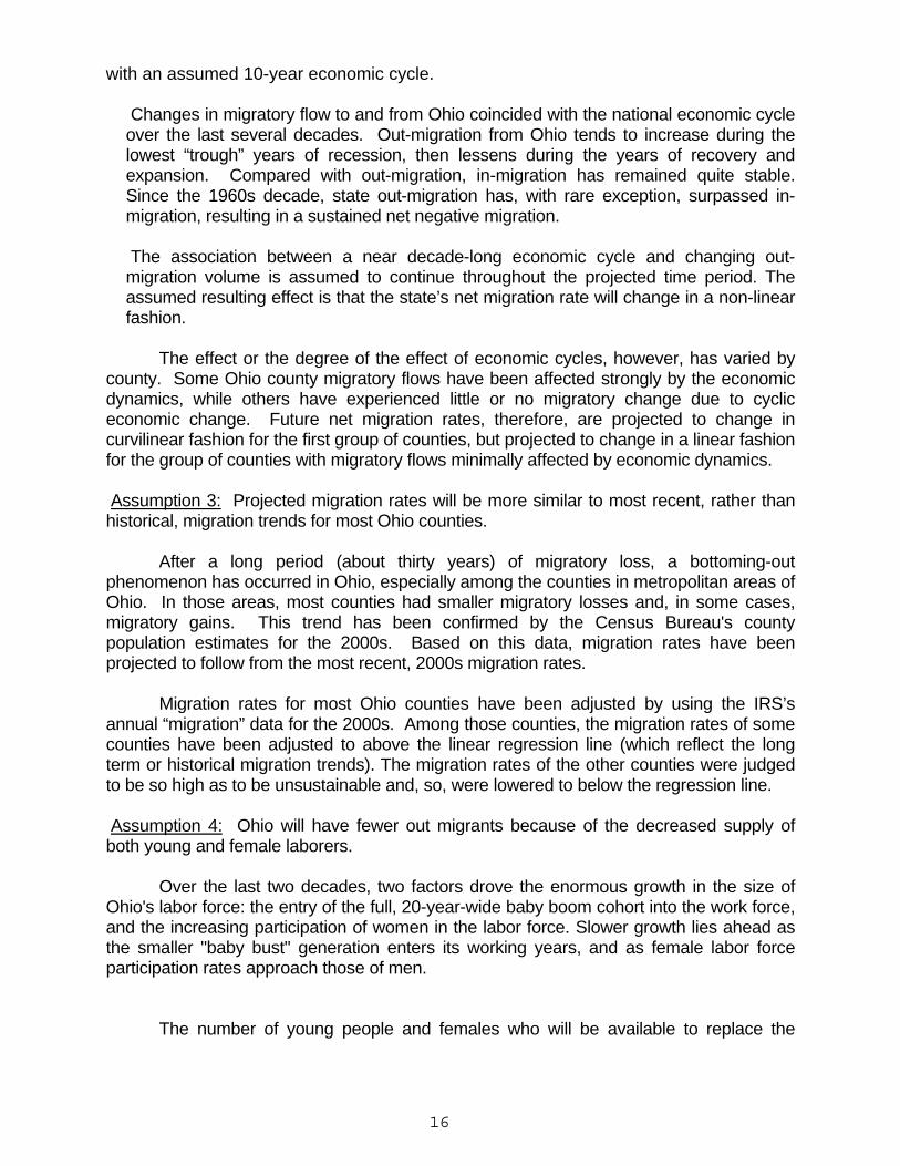
VI. MIGRATION In this projection series, the migration projections were done for Ohio and each county separately. Projected migration trends are based on the most current migration data available and five critical assumptions. This section of the documentation is an explanation of the assumptions and methods employed in making migration projections. This section includes two parts: the first part outlines our migration assumptions; the second part describes the methods employed in projecting migration rates. Migration Assumptions Ohio experienced a net loss of 288,117 persons through migration between 2000 and 2010. The migratory loss between 1980 and 1990 was 621,000 persons, which is the second largest migratory loss in Ohio's history. The largest migratory loss was 635,700 between 1970 and 1980. The net loss through migration between 1990 and 2000 is 63,777 persons. The smaller migration losses reflect Ohio's improved economic and employment conditions in the early 1990's. Therefore, projected Ohio and county net migration continue an improving trend over the projected time period. The projected state migration rates change from -0.7 percent for 2010-2015 period to 1.1 percent for the 2035-2040 period (see Table 3 and Figure 1).

TABLE 3

PROJECTED NET MIGRATION & RATE:

OHIO, 2010-2015 TO 2035-2040

================================== YEAR NET MIGRATION RATE --------- ------------------------ ----------- 00-05 -78,205 -0.69% 05-10 36,267 0.32% 10-15 4,906 0.04% 15-20 44,712 0.40% 20-25 82,331 0.73% 25-30 117,976 1.05% ================================== Data source: Ohio Development Services Agency, Research Office (JH), P.O. Box 1001, Columbus, Ohio 43216-1001, March, 2013

15

Note: The migration rates from 1970-75 to 2005-2010 are the IRS migration rates from the Bureau of Census. The migration rates from 2010-2015 to 2035-2040 are the projected migration rates based on this projection. Assumptions concerning migration trends from 2010 to 2040 for both state and county levels are discussed below. There were four basic assumptions made for projecting future migration trends. Assumption 1: Ohio and counties' future migration rates will follow recent historical (1970-2010) and the most current migration trends. This is a standard projection assumption, based on the logic that the best predictor of short-term future events are the most recent past events. The use of annual Internal Revenue Service data, which provide county-to-county matched filer records for the years 2000-2001 through 2009-2010 allows for the development of a recent migration trend line, to which derived residual migration rates can be applied to provide estimates of age/sex mobility. (Internal Revenue Service, Department of the Treasury, Washington, D.C.) (Appendix 15). Past migration trends for Ohio and each Ohio County are represented by a linear regression line between the initial and terminal periods, calculated by using the migration rates from the previous three decades for each particular county. For Ohio and some Ohio counties with small or moderate changes in migration, future migration rates were adjusted on the past thirty years' (1980-2010) migration trends. For counties with rapid increases or decreases in net migration, forty year (1970-2010) migration trends were used for adjustment. Assumption 2: Population movement occurs within a complex socio-economic environment, and economic conditions create impetus for people to move. Ohio and counties' future net migration rates will vary in curvilinear fashion, in a pattern consistent

‐4.80

‐3.80

‐2.80

‐1.80

‐0.80

0.20

1.20

70‐75 75‐80 80‐85 85‐90 90‐95 95‐00 00‐05 05‐10 10‐15 15‐20 20‐25 25‐30 30‐35 35‐40

Migration Rates:  Ohio, 1970‐2040

16

with an assumed 10-year economic cycle. Changes in migratory flow to and from Ohio coincided with the national economic cycle over the last several decades. Out-migration from Ohio tends to increase during the lowest “trough” years of recession, then lessens during the years of recovery and expansion. Compared with out-migration, in-migration has remained quite stable. Since the 1960s decade, state out-migration has, with rare exception, surpassed in-migration, resulting in a sustained net negative migration. The association between a near decade-long economic cycle and changing out-migration volume is assumed to continue throughout the projected time period. The assumed resulting effect is that the state’s net migration rate will change in a non-linear fashion.

The effect or the degree of the effect of economic cycles, however, has varied by county. Some Ohio county migratory flows have been affected strongly by the economic dynamics, while others have experienced little or no migratory change due to cyclic economic change. Future net migration rates, therefore, are projected to change in curvilinear fashion for the first group of counties, but projected to change in a linear fashion for the group of counties with migratory flows minimally affected by economic dynamics. Assumption 3: Projected migration rates will be more similar to most recent, rather than historical, migration trends for most Ohio counties. After a long period (about thirty years) of migratory loss, a bottoming-out phenomenon has occurred in Ohio, especially among the counties in metropolitan areas of Ohio. In those areas, most counties had smaller migratory losses and, in some cases, migratory gains. This trend has been confirmed by the Census Bureau's county population estimates for the 2000s. Based on this data, migration rates have been projected to follow from the most recent, 2000s migration rates. Migration rates for most Ohio counties have been adjusted by using the IRS’s annual “migration” data for the 2000s. Among those counties, the migration rates of some counties have been adjusted to above the linear regression line (which reflect the long term or historical migration trends). The migration rates of the other counties were judged to be so high as to be unsustainable and, so, were lowered to below the regression line. Assumption 4: Ohio will have fewer out migrants because of the decreased supply of both young and female laborers. Over the last two decades, two factors drove the enormous growth in the size of Ohio's labor force: the entry of the full, 20-year-wide baby boom cohort into the work force, and the increasing participation of women in the labor force. Slower growth lies ahead as the smaller "baby bust" generation enters its working years, and as female labor force participation rates approach those of men. The number of young people and females who will be available to replace the

17

growing number of older retirees will be reduced over the projected years, creating a higher potential for in-state employment. The “baby boomers” also age out of the most mobile 20-39 year-old age groups. If the smaller cohorts temporally following the baby boom migrate at similar rates, the absolute number of migrants will decline So, it is expected that there will be fewer out migrants over the projection period. Migration Projection Methodology The migration component was calculated for each county by multiplying the total county base-year population by the appropriate projected county total net migration rate. Ohio and counties' projected migration rates were based on 2000-2010 gross migration information, as well as the recent historical net migration rates for each county (1980-2000 for most of the Ohio counties and 1970-2000 for the remainder of counties). The projected net migration rates, however, will vary in a curvilinear pattern consistent with an assumed ten-year economic cycle. Each age-sex group's net migration was held constant in proportion to the county's net migration. This proportion was established on the proportion of cohort migrants to county total migrants during 2000-2010 (Ohio and Counties Net Migration by Age and Sex, 2000-2010, The Office of Strategic Research). The migration projections were done for the state and each Ohio County separately. Appendix 16 is a sample of the numerical and graphical migration projections for Ohio and its counties. A step-by-step procedure, consistent with the above assumptions, is outlined below: 1. Obtain a regression line. In this study, the relationship between independent variable x (projected year) and dependent variable y (migration rate) is expressed in the linear regression formula: Y = a + bX To obtain migration rates (y values) for each projected year (x values), a and b values must be calculated first by using previous migration rates. The six previous migration rates (the rates for 1980-1985, 1985-1990 …2000-2010) were employed to calculate a and b values. The migration rates for 1970-1975 and 1975-1980 also went into the calculation for counties with relatively extreme increases or decreases in net migration. Next, each x value (interval between the base and the projected years) was put into the regression equation to obtain the y values (migration rates). For example, the projected migration rate for 2010-2015 is obtained by setting x equal to 30 (2010-1980=30 years) into the regression equation. In this study, the b value (regression coefficient) indicates how much the dependent variable (migration rate) changes as the independent variable (years) changes. As used, the regression line estimates the direction (up or down) of the migration trend as well as the degree of migration rate change (slope of the line).

18

2. Obtain projected migration rates. Since the future migration rates for Ohio and most of Ohio's counties are assumed to change in a non-linear fashion, the projected migration rates will be distributed above the regression line in those five-year periods corresponding to assumed economic cycle peaks, and below in those five-year periods corresponding to economic cycle troughs. Most of Ohio's counties experienced high out-migration to low in-migration (a larger negative value or smaller positive value) for the period 2000-2005, associated with the early-`90s recession. As the economy recovered and began its mid-`2000s expansion, these counties experienced low out-migration to high in-migration (a smaller negative value or larger positive value). Therefore, the estimated migration rates for 2000-2005 and 2005-2010 were used as the high (2000-05) and low (2005-2010) points. The third point is the projected migration rate for the period 2035-2040 (the last y value). A line was drawn between the high point (the y value for 2000-05) and the third point. The y values for each x values for 2010-2015, 2020-2025 and 2030-2035 are located on this line, which shows the migration rates for the projected economic peak years. Another straight line was drawn between the low point (the y value of 2005-2010) and the third point. The y values for each x values for 2015-2020 and 2025-2030 are located on this line, which show the migration rates for the projected recession years. 3. An adjustment of the migration rates was done based on gross migration rates from the end of the 2000s. The projected 2010-2015 county migration rates were forced to align line with the net migration rates of the late 1990's and the estimated 2001 migration rates from the U.S. Bureau of Census. This was accomplished by adjusting the projected target (2035-2040) migration rates until the projected 2010-2015 migration rates matched the most recent migration rates, as well as the estimated 2012 migration rates. 4. Projected migration rates were then reviewed to assure that none surpassed the maximum negative migration rates from the past thirty years. The migration rates for 2000-2005 and 2005-2010 are assumed the largest ones; migration rates of the subsequent projected years are then attenuated, positioned closer and closer to the regression line as time periods move forward. This manner of adjusting the projected rates is the operationalization of our third assumption that future migration rates for Ohio counties will change in a curvilinear fashion, but more and more close to the mean of the trend (the regression line). 5. Age-Sex Cohort Net Migration. Age and sex group migration is dependent on the changing values of the county net migration rates. Each age-sex group's net migration was held constant in proportion to the county's net migration, based on the proportion of cohort migrants to county total migrants during 2000-2010 (Ohio and Counties Net Migration by Age and Sex, 2000-2010, The Office of Strategic Research, Ohio Department of Development). 6. The "plus-minus" adjustment method was used for those counties with extremely high migration proportions for some age groups or/and extremely high and low migration rates

19

for the years of projection. The "plus-minus" method is a proportionate adjustment of a distribution to meet a control total, conforming to a least-squares adjustment of the original frequencies. The marginal total, in this case, is the county's total net migration figure. A procedure that minimizes the adjustment requires the use of two factors, one for the positive items and one for the negative items. The formulas for the factors are as follows: Factors for the positive migration values of ni: { Ó|ni| + (N - n) } / Ó|ni| Factors for the negative migration values of ni: { Ó|ni| - (N - n) } / Ó|ni| where Ó|ni| represents the sum of the absolute values (i.e., without regard to sign) of the original distribution, N is the assigned total (i.e., the projected total net migration), and n is the algebraic sum of the original observations (Shryock, Pg. 546). Appendix 6 is a work sheet illustrating the adjustment procedure of the "plus-minus" method. The "plus-minus" method was used to adjust the cohort migration proportions for the following six counties: Hardin, Jefferson, Lake, Morgan, Portage and Washington. The state level 2000-2010 age/sex proportionate rates of migration were used for four counties -- Athens, Delaware, Franklin and Warren -- because the migration proportions for some age groups for these four counties are so high or so low that even the "plus-minus" method does not sufficiently correct them.

VII. DATA SOURCES The following data were used as input to the calculation program:

-- 2000 and 2010 male and female population in five-year age groups, Census of Population and Housing, 2000 and 2010, U.S. Bureau of the Census;

-- 2000 and 2010 male and female institutional population in five-year age groups, Census of Population and Housing, 2000 and 2010, U.S. Bureau of the Census; -- 2005 estimated population by age, sex, and county, 2006, Population Division, U.S. Bureau of the Census; -- "Student Inventory Data", 2000 and 2010, Ohio Board of Regents, Columbus, Ohio;

-- Live resident births from 2000 and 2010 by single year, county and sex, Vital Statistics (Births), 2000 and 2010, Systems File Specification, Ohio Department of Health, Data Services Division;

-- 2000-2005 and 2005-2010 Age-Specific Fertility Rates by county, The Office

20

Research, Ohio Development Services Agency, Columbus, Ohio, 2012; -- Resident deaths, 2000 and 2010 by single year, county, and sex Vital Statistics (Deaths), 2000 and 2010, Systems File Specification, Ohio Department of Health, Data Services Division; -- Revised National Census 2000-2005 Age/Sex-Specific Survival Rates by county, The Office of Research, Ohio Development Services Agency, Columbus, Ohio, 2012; -- IRS state and county migration flows, 2000 and 2010, Internal Revenue Service (IRS), U.S. Bureau of the Census;

-- Estimated 2000 and 2010 age/sex-specific net migration rates and proportion of migrants, "Net Migration: Ohio and Counties, By Age, Sex and Race: 2000 and 2010 ", The Research Office, Ohio Development Services Agency, Columbus, Ohio, 2012;

-- "Ohio and Counties, Net Migration By Age and Sex: 1990 to 2000", Ohio Data Users Center, Ohio Department of Development, Columbus, Ohio, 1995;

-- "Ohio and Counties, Net Migration By Age and Sex: 1980 to 1990", Ohio Data Users Center, Ohio Department of Development, Columbus, Ohio, 1995; -- "Net Migration of the Population, 1970-80, by Age, Sex, and Color: Part 2-- North Central States", Economic Research Service, U.S. Department of Agriculture, Institute for Behavioral Research, University of Georgia and Research Applied to National Needs, National Science Foundation, The University of Georgia Printing Department, Athens, Georgia, 1985; -- "Net Migration of the Population, 1960-1970", Economic Research Service, U.S. Department of Agriculture, Research Foundation, Oklahoma State University and Area Redevelopment Administration, U.S. Department of Commerce, Washington, D.C., U.S. Government Printing Office, 1975; -- Projected 2010-2015 to 2035-2040 Net Migration Rates by County, The Office Research, Ohio Development Services Agency, Columbus, Ohio, 2012.