Polymorphic versus MonomorphicFlow-insensitive Points-to Analysis for C†

Jeffrey S. Foster1, Manuel Fahndrich2, and Alexander Aiken1

1 University of California, Berkeley, 387 Soda Hall #1776, Berkeley, CA 94720{jfoster,aiken}@cs.berkeley.edu

2 Microsoft Research, One Microsoft Way, Redmond, WA 98052maf@microsoft.com

Abstract We carry out an experimental analysis for two of the de-sign dimensions of flow-insensitive points-to analysis for C: polymorphicversus monomorphic and equality-based versus inclusion-based. Holdingother analysis parameters fixed, we measure the precision of the four de-sign points on a suite of benchmarks of up to 90,000 abstract syntax treenodes. Our experiments show that the benefit of polymorphism variessignificantly with the underlying monomorphic analysis. For our equality-based analysis, adding polymorphism greatly increases precision, whilefor our inclusion-based analysis, adding polymorphism hardly makes anydifference. We also gain some insight into the nature of polymorphismin points-to analysis of C. In particular, we find considerable polymor-phism available in function parameters, but little or no polymorphism infunction results, and we show how this observation explains our results.

1 Introduction

When constructing a constraint-based program analysis, the analysis designermust weigh the costs and benefits of many possible design points. Two importanttradeoffs are:

– Is the analysis polymorphic or monomorphic? A polymorphic analysis sepa-rates analysis information by call site, while monomorphic analysis conflatesall call sites. A polymorphic analysis is more precise but also more expensivethan a corresponding monomorphic analysis.

– What is the underlying constraint relation? Possibilities include equalities(solved with unification) or more precise and expensive inclusions (solvedwith dynamic transitive closure), among many others.

Intuitively, if we want the greatest possible precision, we should use a poly-morphic inclusion-based analysis, while if we are mostly concerned with effi-ciency, we should use a monomorphic equality-based analysis. But how much† This research was supported in part by the National Science Foundation Young

Investigator Award No. CCR-9457812, NASA Contract No. NAG2-1210, an NDSEGfellowship, and an equipment donation from Intel.

MonomorphicSteensgaard’s

PolymorphicSteensgaard’s

MonomorphicAndersen’s

PolymorphicAndersen’s

���+

QQQs

QQQs

���+

Figure 1. Relation between the four analyses. There is an edge from analysis x toanalysis y if y is at least as precise as x.

more precision does polymorphism add, and what do we lose by using equal-ity constraints? In this paper, we try to answer these questions for a particularconstraint-based program analysis, flow-insensitive points-to analysis for C. Ourgoal is to compare the tradeoffs between the four possible combinations of poly-morphism/monomorphism and equality constraints/inclusion constraints.

Points-to analysis computes, for each expression in a C program, a set ofabstract memory locations (variables and heap) to which the expression couldpoint. Our monomorphic inclusion-based analysis (Sect. 4.1) implements a ver-sion of Andersen’s points-to analysis [4], and our monomorphic equality-basedanalysis (Sect. 4.2) implements a version of Steensgaard’s points-to analysis [29].To add polymorphism to Andersen’s and Steensgaard’s analyses (Sect. 4.3), weuse Hindley-Milner style parametric polymorphism [21].

Our analyses are designed such that monomorphic Andersen’s analysis is atleast as precise as monomorphic Steensgaard’s analysis [16, 28], and similarlyfor the polymorphic versions. Given the construction of our analyses, it is atheorem that the hierarchy of precision shown in Fig. 1 always holds. The maincontribution of this work is the quantification of the exact relationship amongthese analyses. A secondary contribution of this paper is the development ofpolymorphic versions of Andersen’s and Steensgaard’s points-to analyses.

Running the analyses on our suite of benchmarks, we find the following results(see Sect. 5), where � is read “is significantly less precise than.” In general,

Monomorphic Steensgaard’s�Polymorphic Steensgaard’s�

Polymorphic Andersen’s

Monomorphic Steensgaard’s�Monomorphic Andersen’s ≈Polymorphic Andersen’s

The exact relationships vary from benchmark to benchmark. These results arerather surprising—why should polymorphism not add much precision to Ander-sen’s analysis but benefit Steensgaard’s analysis? While we do not have definitiveanswers to these questions, Sect. 5.3 suggests some possible explanations.

Notice from this table that monomorphic Andersen’s analysis is approxi-mately as precise as polymorphic Andersen’s analysis, while polymorphic Steens-gaard’s analysis is much less precise than polymorphic Andersen’s analysis. Note,however, that polymorphic Steensgaard’s analysis and monomorphic Andersen’sanalysis are in general incomparable (see Sect. 5.1). Still, given that polymorphicanalyses are much more complicated to understand, reason about, and imple-ment than their monomorphic counterparts, these results suggest that monomor-phic Andersen’s analysis may represent the best design choice among the fouranalyses. This may be a general principle: in order to improve a program analysis,developing a more powerful monomorphic analysis may be preferable to addingcontext-sensitivity, one example of which is Hindley-Milner style polymorphism.

Carrying out an experimental exploration of even a portion of the designspace for non-trivial program analyses is a painstaking task. In interpreting ourresults there are two important things to keep in mind. First, our exploration ofeven the limited design space of flow-insensitive points-to analysis for C is stillpartial—there are dimensions other than the two that we explore that may notbe orthogonal and may lead to different tradeoffs. For example, it may matterhow precisely heap memory is modeled, how strings are modeled, whether Cstructs are analyzed by field or all fields are summarized together, and so on.Section 5 details our choices for these parameters. Also, Hindley-Milner stylepolymorphism is only one way to add context-sensitivity to a points-to analy-sis, and other approaches (e.g., polymorphic recursion [15]) may yield differenttradeoffs.

Second, our experiments measure the relative precision of each analysis. Theydo not measure the relative impact of each analysis in a compiler. For example, itmay be that some points-to sets are more important than others to an optimizer,and thus increases in precision may not always lead to better optimizations. How-ever, a more precise analysis should not lead to worse optimizations than a lessprecise analysis. We should also point out that it is difficult to separate the bene-fit of a pointer analysis in a compiler from the design of the rest of the optimizer.Measures of relative precision have the advantage of being independent of thespecific choices made in using the analysis information by a particular tool.

2 Related Work

Andersen’s [4] and Steensgaard’s [29] points-to analyses are only two choices ina vast array of possible alias analyses, among them [5, 6, 7, 8, 9, 10, 11, 15, 19,20, 27, 28, 31, 33, 34]. As our results suggest, the benefit of polymorphism (moregenerally, context-sensitivity) may vary greatly with the particular analysis.

Hindley-Milner style polymorphism [21] has been studied extensively. Theonly direct applications of Hindley-Milner polymorphism to C of which we are

aware are the analyses in this paper, the polymorphic recursive analysis proposedin [15] (see below), and the Lackwit system [23]. Lackwit, a software engineeringtool, computes ML-style types for C and appears to scale very well to largeprograms.

Mossin [22] develops a polymorphic flow analysis based on polymorphic re-cursion and atomic subtyping constraints. Mossin’s system starts with a type-annotated program and infers atomic flow constraints, whereas we infer the typeand flow annotations simultaneously and do not have an atomic subtyping sys-tem. [15] develops an efficient algorithm for both subtyping and equality-basedpolymorphic recursive flow analyses, and shows how to construct a polymorphicrecursive version of Steensgaard’s analysis. (In contrast, in this paper we useHindley-Milner style polymorphism, which can be less precise.) We believe thatthe techniques of [15] can also be adapted to Andersen’s analysis.

Other research has explored making monomorphic inclusion-based analysesscalable. [14] describes an online cycle-elimination algorithm for simplifying in-clusion constraints. [30] describes a related optimization technique, projectionmerging, which merges multiple projections of the same set variable. Our cur-rent implementation uses both of these techniques, which makes it possible torun the polymorphic inclusion-based analysis on our larger benchmarks.

Finally, we discuss a selection of related analyses. Wilson and Lam [31] pro-pose a flow-sensitive alias analysis that distinguishes calls to the same functionin different aliasing contexts. Their system analyzes a function once for eachaliasing pattern of its actual parameters. In contrast, we analyze each functiononly once, independently of its context, by constructing types that summarizefunctions’ points-to effects in any context.

Ruf [26] studies the tradeoff between context-sensitivity and context-insen-sitivity for a particular dataflow-style alias analysis, discovering that context-sensitivity makes little appreciable difference in the accuracy of the results. Ourresults partially agree with his. For Andersen’s inclusion-based analysis we findthe same trend. However, for Steensgaard’s equality-based analysis, which issubstantially less precise than Ruf’s analysis, adding polymorphism makes asignificant difference

Emami, Ghiya, and Hendren [11] propose a flow-sensitive, context-sensitiveanalysis. The scalability of this analysis is unknown.

Landi and Ryder [20] study a very precise flow-sensitive, context-sensitiveanalysis. Their flow-sensitive system has difficulty scaling to large programs;recent work has focused on combined analyses that apply different alias analysesto different parts of a program [35].

Chatterjee, Ryder, and Landi [6] propose an analysis for Java and C++ thatuses a flow-sensitive analysis with conditional points-to relations whose validitydepends on the aliasing and type information provided by the context. Whilethe style of polymorphism used in [6] appears related to Hindley-Milner stylepolymorphism, the exact relationship is unclear.

Das [7] proposes a monomorphic alias analysis with precision close to An-dersen’s analysis but cost close to Steensgaard’s analysis. The effect of adding

polymorphism to Das’s analysis is currently unknown but cannot yield moreprecision than polymorphic Andersen’s analysis.

3 Constraints

Our analyses are formulated as non-standard type systems for C. We followthe usual approach for constraint-based program analysis: As the analyses infertypes for a program’s expressions, a system of typing constraints is generatedon the side. The solution to the constraints defines the points-to graph of theprogram.

Our analyses are implemented with the Berkeley Analysis Engine (BANE)[1], which is a framework for constructing constraint-based analyses. BANE sup-ports analyses involving multiple sorts of constraints, two of which are used byour points-to analyses. Our implementation of Andersen’s analysis uses inclusion(or set) constraints [2, 18]. Our implementation of Steensgaard’s analysis uses amixture of equality (or term) and inclusion constraints. The rest of this sectionprovides background on the constraint formalisms.

Each sort of constraint comes equipped with a constraint relation. The rela-tion between set expressions is ⊆, and the relation between term expressions is=. For our purposes, set expressions se consist of set variables X ,Y, . . . from afamily of variables Vars (caligraphic text denotes variables), terms constructedfrom n-ary constructors c ∈ Con, a special form proj (c, i, se), an empty set 0,and a universal set 1.

se ::= X | c(se1, . . . , sen) | proj (c, i, se) | 0 | 1

Similarly, term expressions are of the form

te ::= X | c(te1, . . . , ten) | 0

Here 0 represents a special, distinguished nullary constructor.Each constructor c is given a signature Sc specifying the arity, variance, and

sort of c. If S is the set of sorts (in this case, S = {Term,Set}), then constructorsignatures are of the form

c : ι1 × · · · × ιarity(c) → S

where ιi is s (covariant) or s (contravariant) for some s ∈ S. Intuitively, a con-structor c is covariant in an argument X if the set denoted by a term c(. . . ,X , . . .)becomes larger as X increases. Similarly, a constructor c is contravariant in anargument X if the set denoted by a term c(. . . ,X , . . .) becomes smaller as Xincreases. To improve readability, we mark contravariant arguments with over-bars.

One example constructor from Andersen’s analysis is

lam : Set×Set× Set→ Set

The lam constructor models function types. The first (covariant) argument namesthe function, the second (contravariant) argument represents the domain, andthe third (covariant) argument represents the range.

Steensgaard’s analysis uses a constructor

ref : Set×Term×Term→ Term

to model locations. The first field models the set of aliases of this location, andthe second and third fields model the contents of this location. See Sect. 4.2 fora discussion of why a set is needed for the first field. More discussion of mixedconstraints can be found in [12, 13].

Our system also includes conditional equality constraints L ≤ R (defined onterms) to support Steensgaard’s analysis (see Sect. 4.2). The constraint L ≤ Rholds if either L = R or L = 0 holds. Intuitively, if L is ever unified with aconstructed term, then the constraint L ≤ R becomes L = R. Otherwise L ≤ Rmakes no constraint on R.

Our language of set constraints has no explicit operation to select componentsof a constructor. Instead we use constraints of the form

L ⊆ c(. . . ,Yi, . . .) (∗)

to make Yi contain c−i(L) if c is covariant in i, and to make c−i(L) contain Yiif c is contravariant in i. However, such a constraint is inconsistent if L containsterms whose head constructor is not c. To overcome this limitation, we defineconstraints of the form

L ⊆ proj (c, i,Yi)This constraint has the same effect as (∗) on the elements of L constructed withc, and no effect on the other elements of L.

Solving a system of constraints involves computing an explicit solved form ofall solutions or of a particular solution. See [3, 12, 13] for a thorough discussionof the constraint solver used in BANE.

4 The Analyses

This section develops monomorphic and polymorphic versions of Andersen’s andSteensgaard’s analyses. The presentation of the monomorphic version of Ander-sen’s analysis mostly follows [14, 30] and is given primarily to make the paperself contained.

For a C program, points-to analysis computes a set of abstract memory loca-tions (variables and heap) to which each expression could point. Andersen’s andSteensgaard’s analyses compute a points-to graph [11]. Graph nodes representabstract memory locations, and there is an edge from a node x to a node y ifx may contain a pointer to y. Informally, the analyses begin with some initialpoints-to relationships and close the graph under the rule

For an assignment e1 = e2, anything in the points-to set for e2 must alsobe in the points-to set for e1.

a = &b;

a = &c;

*a = &d;

a

b

d

c

����1

PPPPq

PPPPq

����1 a b,c d- -

(a) Andersen’s Analysis (b) Steensgaard’s Analysis

Figure 2. Example points-to graph

For Andersen’s analysis, each node in the points-to graph may have directededges to any number of other nodes. For Steensgaard’s analysis, each node mayhave at most one out-edge, and graph nodes are coalesced if necessary to enforcethis requirement. Figure 2 shows the points-to graph for a simple C programcomputed by Andersen’s analysis (a) and Steensgaard’s analysis (b).

4.1 Andersen’s Analysis

In Andersen’s analysis, types τ represent sets of abstract memory locations andare described by the following grammar:

ρ ::= Px | lxτ ::= X | ref (ρ, τ, τ) | lam(ρ, τ , τ)

Here the constructor signatures are

ref : Set×Set×Set→ Setlam : Set×Set× Set→ Set

X and Px are set variables, and lx is a constant (a constructor of arity 0).Contravariant arguments are marked with overbars. Note that function typeslam(· · ·) are contravariant in the domain (second argument) and covariant inthe range (third argument).

Memory locations can be thought of as abstract data types with two oper-ations, one to get the value stored in the location and one to set it. Intuitively,the get and set operations have types

– get : void→ X– set : X → void

where X is the type of data held in the memory location. Dereferencing a locationcorresponds to applying the get operation, and updating a location correspondsto applying the set operation. Note that the type variable X appears covari-antly in the type of the get operation and contravariantly in the type of the setoperation.

Translating this intuition into a set constraint formulation, the location of avariable x is modeled with the type ref (lx,X ,X ), where lx is a constant repre-senting the name of the location, the covariant occurrence of X represents theget method, and the contravariant occurrence of X (marked with an overbar)represents the set method. For convenience, we choose not to represent the voidcomponents of the get and set methods’ types.

We also associate with each location x a set variable Px and add the con-straints X ⊆ proj (ref , 1,Px) and X ⊆ proj (lam, 1,Px). This constrains Px tocontain the set of abstract locations, including functions, in the points-to set X .The points-to graph is then defined by the least solution of Px for every locationx. In the set formulation, the least solution for the points-to graph shown inFig. 2a is

Pa = {lb, lc} Pb = {ld} Pc = {ld}

In addition to reference types we also must model function types, since Callows pointers to functions to be stored in memory. The type lam(lf, τ1, τ2)represents the function named f (every C function has a name) with argumentτ1 and return value τ2. For simplicity the grammar allows only one argument. Inour implementation, arguments are modeled with an ordered record {τ1, . . . , τn}[25].1

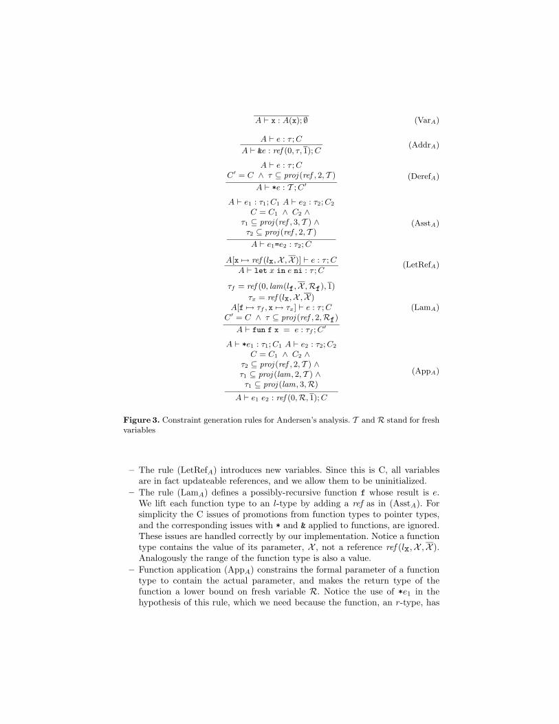
Figure 3 shows a fragment of the type rules for the monomorphic versionof Andersen’s analysis. Judgments are of the form A ` e : τ ;C, meaning thatin typing environment A, expression e has type τ under the constraints C. Forsimplicity we present only the interesting type rules. The full rules for all of Ccan be found in [16].

We briefly discuss the rules. To avoid having separate rules for l- and r-values, we model all variables as l-types. Thus the type of a variable x is ourrepresentation of its location, i.e., a ref type.

– Rule (VarA) states that typings in the environment trivially hold.– The address-of operator (AddrA) adds a level of indirection to its operand

by adding a ref constructor. The location (first) and set (third) fields of theresulting type are 0 and 1, respectively, because &e is not itself an l-valueand cannot be updated.

– The dereferencing operator (DerefA) removes a ref and makes the freshvariable T a superset of the points-to set of τ . Note the use of proj in caseτ also contains a function type.

– The assignment rule (AsstA) uses the same technique as (DerefA) to get thecontents of the right-hand side, and then uses the contravariant set field ofthe ref constructor to store the contents in the left-hand side location. See[16] for detailed explanations and examples.

1 Note that we do not handle variable-length argument lists (varargs) correctly evenwith records. Handling varargs requires compiler- and architecture-specific knowl-edge of the layout of parameters in memory. See Sect. 5.

A ` x : A(x); ∅ (VarA)

A ` e : τ ;C

A ` &e : ref (0, τ, 1);C(AddrA)

A ` e : τ ;CC′ = C ∧ τ ⊆ proj (ref , 2, T )

A ` *e : T ;C′(DerefA)

A ` e1 : τ1;C1 A ` e2 : τ2;C2

C = C1 ∧ C2 ∧τ1 ⊆ proj (ref , 3, T ) ∧τ2 ⊆ proj (ref , 2, T )

A ` e1=e2 : τ2;C

(AsstA)

A[x 7→ ref (lx,X ,X )] ` e : τ ;C

A ` let x in e ni : τ ;C(LetRefA)

τf = ref (0, lam(lf,X ,Rf), 1)

τx = ref (lx,X ,X )A[f 7→ τf , x 7→ τx] ` e : τ ;C

C′ = C ∧ τ ⊆ proj (ref , 2,Rf)

A ` fun f x = e : τf ;C′

(LamA)

A ` *e1 : τ1;C1 A ` e2 : τ2;C2

C = C1 ∧ C2 ∧τ2 ⊆ proj (ref , 2, T ) ∧τ1 ⊆ proj (lam, 2, T ) ∧τ1 ⊆ proj (lam, 3,R)

A ` e1 e2 : ref (0,R, 1);C

(AppA)

Figure 3. Constraint generation rules for Andersen’s analysis. T and R stand for freshvariables

– The rule (LetRefA) introduces new variables. Since this is C, all variablesare in fact updateable references, and we allow them to be uninitialized.

– The rule (LamA) defines a possibly-recursive function f whose result is e.We lift each function type to an l-type by adding a ref as in (AsstA). Forsimplicity the C issues of promotions from function types to pointer types,and the corresponding issues with * and & applied to functions, are ignored.These issues are handled correctly by our implementation. Notice a functiontype contains the value of its parameter, X , not a reference ref (lx,X ,X ).Analogously the range of the function type is also a value.

– Function application (AppA) constrains the formal parameter of a functiontype to contain the actual parameter, and makes the return type of thefunction a lower bound on fresh variable R. Notice the use of *e1 in thehypothesis of this rule, which we need because the function, an r-type, has

been lifted to an l-type in (LamS). The result R, which is an r-type, is liftedto an l-type by adding a ref constructor, as in (AddrA).

4.2 Steensgaard’s Analysis

Intuitively, Steensgaard’s analysis replaces the inclusion constraints of Ander-sen’s analysis with equality constraints. The type language is a small modifica-tion of the previous system:

ρ ::= Px | Lx | lxτ ::= X | ref (ρ, τ, η)η ::= X | lam(τ, τ)

with constructor signatures

ref : Set×Term×Term→ Termlam : Term×Term→ Term

As before, ρ denotes locations and τ denotes updateable references. Following[29], in this system function types η are always structurally within ref (· · ·) typesbecause in a system of equality constraints we cannot express a union ref (. . .)∪lam(. . .). For a similar reason location sets ρ consist solely of variables Px or Lxand are modeled as sets (see below).

Each program variable x is modeled with the type ref (Lx,X ,Fx), where Lxis a Set variable. For each location x we add a constraint lx ⊆ Lx, where lx is anullary constructor (as in Andersen’s analysis). We also associate with locationx another set variable Px and add the constraint X ≤ ref (Px, ∗, ∗), where ∗stands for a fresh unnamed variable.

We compute the points-to graph by finding the least solution of the Pxvariables. For the points-to graph in Fig. 2b, the result is

Pa = {lb, lc} Pb = {ld} Pc = {ld}

Notice that b and c are inferred to be aliased, i.e., Lb = Lc. If we had insteadused nullary constructors directly in the ρ field of ref , or had the ρ field been aTerm sort, then the constraints would have been inconsistent, since lb 6= lc.

In Steensgaard’s formulation [29], the relation between locations x and theircorresponding term variables Px is implicit. While this suffices for a monomor-phic analysis, in a polymorphic analysis maintaining this map is problematic, asgeneralization, simplification, and instantiation (see Sect. 4.3) all cause variablesto be renamed.

Mixed constraints provide an elegant solution to this problem. By explicitlyrepresenting the mapping from locations to location names in a constraint for-mulation, we guarantee that any sound constraint manipulations preserve thismapping.

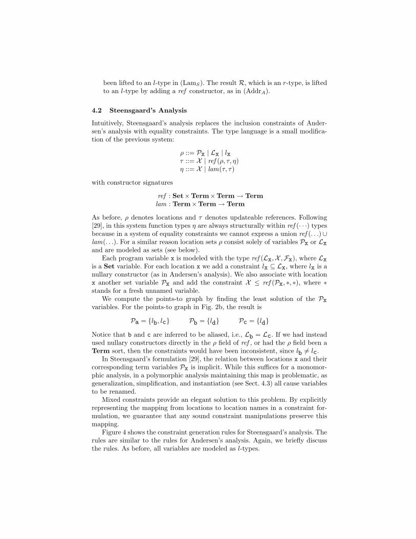
Figure 4 shows the constraint generation rules for Steensgaard’s analysis. Therules are similar to the rules for Andersen’s analysis. Again, we briefly discussthe rules. As before, all variables are modeled as l-types.

A ` x : A(x); ∅ (VarS)

A ` e : τ ;C

A ` &e : ref (∗, τ, ∗);C (AddrS)

A ` e : τ ;CC′ = C ∧ τ ≤ ref (∗, T , ∗)

A ` *e : T ;C′(DerefS)

A ` e1 : τ1;C1 A ` e2 : τ2;C2

C = C1 ∧ C2 ∧τ1 ≤ ref (∗, T1, ∗) ∧ τ2 ≤ ref (∗, T2, ∗) ∧

T2 ≤ T1

A ` e1=e2 : τ2;C

(AsstS)

A[x 7→ ref (Lx,X ,Fx)] ` e : τ ;C

A ` let x in e ni : τ ;C(LetRefS)

τf = ref (∗, ref (Lf, Tf, lam(X ,Rf)), ∗)τx = ref (Lx,X ,Fx)

A[f 7→ τf , x 7→ τx] ` e : τ ;CC′ = C ∧ τ ≤ ref (∗, T , ∗) ∧ T ≤ Rf

A ` fun f x = e : τf ;C′

(LamS)

A ` *e1 : τ1;C1 A ` e2 : τ2;C2

C = C1 ∧ C2 ∧τ1 ≤ ref (∗, ∗,F) ∧ F ≤ lam(Y,R) ∧

τ2 ≤ ref (∗, T , ∗) ∧ T ≤ YA ` e1 e2 : ref (∗,R, ∗);C

(AppS)

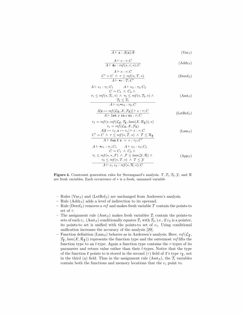
Figure 4. Constraint generation rules for Steensgaard’s analysis. T , T1, T2,Y, and Rare fresh variables. Each occurrence of ∗ is a fresh, unnamed variable

– Rules (VarS) and (LetRefS) are unchanged from Andersen’s analysis.– Rule (AddrS) adds a level of indirection to its operand.– Rule (DerefS) removes a ref and makes fresh variable T contain the points-to

set of τ .– The assignment rule (AsstS) makes fresh variables Ti contain the points-to

sets of each ei. (AsstS) conditionally equates T1 with T2, i.e., if e2 is a pointer,its points-to set is unified with the points-to set of e1. Using conditionalunification increases the accuracy of the analysis [29].

– Function definition (LamS) behaves as in Andersen’s analysis. Here, ref (Lf,Tf, lam(X ,Rf)) represents the function type and the outermost ref lifts thefunction type to an l-type. Again a function type contains the r-types of itsparameter and return value rather than their l-types. Notice that the typeof the function f points to is stored in the second (τ) field of f’s type τf, notin the third (η) field. Thus in the assignment rule (AsstS), the Ti variablescontain both the functions and memory locations that the ei point to.

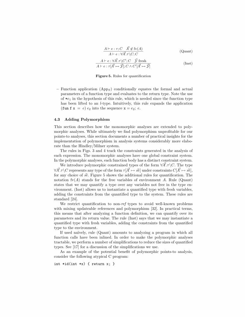
A ` e : τ ;C ~X 6∈ fv(A)

A ` e : ∀ ~X .τ\C;C(Quant)

A ` e : ∀ ~X .τ\C′;C ~Y fresh

A ` e : τ [ ~X 7→ ~Y];C ∧ C′[ ~X 7→ ~Y](Inst)

Figure 5. Rules for quantification

– Function application (AppS) conditionally equates the formal and actualparameters of a function type and evaluates to the return type. Note the useof *e1 in the hypothesis of this rule, which is needed since the function typehas been lifted to an l-type. Intuitively, this rule expands the application(fun f x = e) e2 into the sequence x = e2; e.

4.3 Adding Polymorphism

This section describes how the monomorphic analyses are extended to poly-morphic analyses. While ultimately we find polymorphism unprofitable for ourpoints-to analyses, this section documents a number of practical insights for theimplementation of polymorphism in analysis systems considerably more elabo-rate than the Hindley/Milner system.

The rules in Figs. 3 and 4 track the constraints generated in the analysis ofeach expression. The monomorphic analyses have one global constraint system.In the polymorphic analyses, each function body has a distinct constraint system.

We introduce polymorphic constrained types of the form ∀ ~X .τ\C. The type∀ ~X .τ\C represents any type of the form τ [ ~X 7→ ~se] under constraints C[ ~X 7→ ~se],for any choice of ~se. Figure 5 shows the additional rules for quantification. Thenotation fv(A) stands for the free variables of environment A. Rule (Quant)states that we may quantify a type over any variables not free in the type en-vironment. (Inst) allows us to instantiate a quantified type with fresh variables,adding the constraints from the quantified type to the system. These rules arestandard [24].

We restrict quantification to non-ref types to avoid well-known problemswith mixing updateable references and polymorphism [32]. In practical terms,this means that after analyzing a function definition, we can quantify over itsparameters and its return value. The rule (Inst) says that we may instantiate aquantified type with fresh variables, adding the constraints from the quantifiedtype to the environment.

If used naıvely, rule (Quant) amounts to analyzing a program in which allfunction calls have been inlined. In order to make the polymorphic analysestractable, we perform a number of simplifications to reduce the sizes of quantifiedtypes. See [17] for a discussion of the simplifications we use.

As an example of the potential benefit of polymorphic points-to analysis,consider the following atypical C program:

int *id(int *x) { return x; }

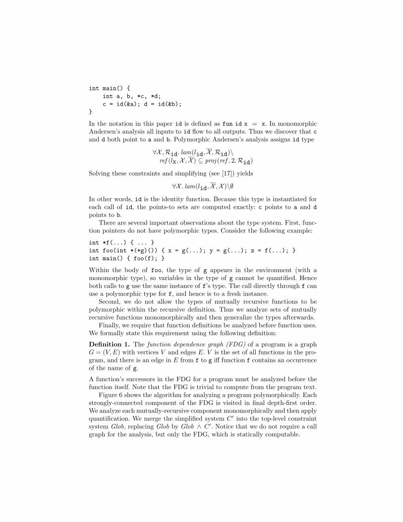
int main() {int a, b, *c, *d;c = id(&a); d = id(&b);

}

In the notation in this paper id is defined as fun id x = x. In monomorphicAndersen’s analysis all inputs to id flow to all outputs. Thus we discover that cand d both point to a and b. Polymorphic Andersen’s analysis assigns id type

∀X ,Rid. lam(lid,X ,Rid)\ref (lx,X ,X ) ⊆ proj (ref , 2,Rid)

Solving these constraints and simplifying (see [17]) yields

∀X . lam(lid,X ,X )\∅

In other words, id is the identity function. Because this type is instantiated foreach call of id, the points-to sets are computed exactly: c points to a and dpoints to b.

There are several important observations about the type system. First, func-tion pointers do not have polymorphic types. Consider the following example:

int *f(...) { ... }int foo(int *(*g)()) { x = g(...); y = g(...); z = f(...); }int main() { foo(f); }

Within the body of foo, the type of g appears in the environment (with amonomorphic type), so variables in the type of g cannot be quantified. Henceboth calls to g use the same instance of f’s type. The call directly through f canuse a polymorphic type for f, and hence is to a fresh instance.

Second, we do not allow the types of mutually recursive functions to bepolymorphic within the recursive definition. Thus we analyze sets of mutuallyrecursive functions monomorphically and then generalize the types afterwards.

Finally, we require that function definitions be analyzed before function uses.We formally state this requirement using the following definition:

Definition 1. The function dependence graph (FDG) of a program is a graphG = (V,E) with vertices V and edges E. V is the set of all functions in the pro-gram, and there is an edge in E from f to g iff function f contains an occurrenceof the name of g.

A function’s successors in the FDG for a program must be analyzed before thefunction itself. Note that the FDG is trivial to compute from the program text.

Figure 6 shows the algorithm for analyzing a program polymorphically. Eachstrongly-connected component of the FDG is visited in final depth-first order.We analyze each mutually-recursive component monomorphically and then applyquantification. We merge the simplified system C ′ into the top-level constraintsystem Glob, replacing Glob by Glob ∧ C ′. Notice that we do not require a callgraph for the analysis, but only the FDG, which is statically computable.

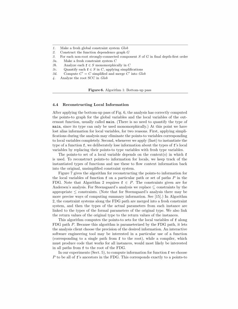
1. Make a fresh global constraint system Glob2. Construct the function dependence graph G3. For each non-root strongly-connected component S of G in final depth-first order3a. Make a fresh constraint system C3b. Analyze each f ∈ S monomorphically in C3c. Quantify each f ∈ S in C, applying simplifications3d. Compute C′ = C simplified and merge C′ into Glob4. Analyze the root SCC in Glob

Figure 6. Algorithm 1: Bottom-up pass

4.4 Reconstructing Local Information

After applying the bottom-up pass of Fig. 6, the analysis has correctly computedthe points-to graph for the global variables and the local variables of the out-ermost function, usually called main. (There is no need to quantify the type ofmain, since its type can only be used monomorphically.) At this point we havelost alias information for local variables, for two reasons. First, applying simpli-fications during the analysis may eliminate the points-to variables correspondingto local variables completely. Second, whenever we apply (Inst) to instantiate thetype of a function f, we deliberately lose information about the types of f’s localvariables by replacing their points-to type variables with fresh type variables.

The points-to set of a local variable depends on the context(s) in which fis used. To reconstruct points-to information for locals, we keep track of theinstantiated types of functions and use these to flow context information backinto the original, unsimplified constraint system.

Figure 7 gives the algorithm for reconstructing the points-to information forthe local variables of function f on a particular path or set of paths P in theFDG. Note that Algorithm 2 requires f ∈ P . The constraints given are forAndersen’s analysis. For Steensgaard’s analysis we replace ⊆ constraints by theappropriate ≤ constraints. (Note that for Steensgaard’s analysis there may bemore precise ways of computing summary information. See [15].) In Algorithm2, the constraint systems along the FDG path are merged into a fresh constraintsystem, and then the types of the actual parameters from each instance arelinked to the types of the formal parameters of the original type. We also linkthe return values of the original type to the return values of the instances.

This algorithm computes the points-to sets for the local variables of f alongFDG path P . Because this algorithm is parameterized by the FDG path, it letsthe analysis client choose the precision of the desired information. An interactivesoftware engineering tool may be interested in a particular use of a function(corresponding to a single path from f to the root), while a compiler, whichmust produce code that works for all instances, would most likely be interestedin all paths from f to the root of the FDG.

In our experiments (Sect. 5), to compute information for function f we chooseP to be all of f’s ancestors in the FDG. This corresponds exactly to a points-to

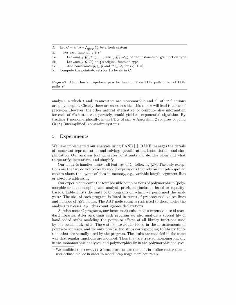
1. Let C = Glob ∧∧g∈P Cg be a fresh system

2. For each function g ∈ P2a. Let lam(lg,G1,R1), . . . , lam(lg,Gn,Rn) be the instances of g’s function type.

2b. Let lam(lg,G,R) be g’s original function type2c. Add constraints Gi ⊆ G and R ⊆ Ri for i ∈ [1..n].3. Compute the points-to sets for f’s locals in C.

Figure 7. Algorithm 2: Top-down pass for function f on FDG path or set of FDGpaths P

analysis in which f and its ancestors are monomorphic and all other functionsare polymorphic. Clearly there are cases in which this choice will lead to a loss ofprecision. However, the other natural alternative, to compute alias informationfor each of f’s instances separately, would yield an exponential algorithm. Bytreating f monomorphically, in an FDG of size n Algorithm 2 requires copyingO(n2) (unsimplified) constraint systems.

5 Experiments

We have implemented our analyses using BANE [1]. BANE manages the detailsof constraint representation and solving, quantification, instantiation, and sim-plification. Our analysis tool generates constraints and decides when and whatto quantify, instantiate, and simplify.

Our analysis handles almost all features of C, following [29]. The only excep-tions are that we do not correctly model expressions that rely on compiler-specificchoices about the layout of data in memory, e.g., variable-length argument listsor absolute addressing.

Our experiments cover the four possible combinations of polymorphism (poly-morphic or monomorphic) and analysis precision (inclusion-based or equality-based). Table 1 lists the suite of C programs on which we performed the anal-yses.2 The size of each program is listed in terms of preprocessed source linesand number of AST nodes. The AST node count is restricted to those nodes theanalysis traverses, e.g., this count ignores declarations.

As with most C programs, our benchmark suite makes extensive use of stan-dard libraries. After analyzing each program we also analyze a special file ofhand-coded stubs modeling the points-to effects of all library functions usedby our benchmark suite. These stubs are not included in the measurements ofpoints-to set sizes, and we only process the stubs corresponding to library func-tions that are actually used by the program. The stubs are modeled in the sameway that regular functions are modeled. Thus they are treated monomorphicallyin the monomorphic analyses, and polymorphically in the polymorphic analyses.2 We modified the tar-1.11.2 benchmark to use the built-in malloc rather than a

user-defined malloc in order to model heap usage more accurately.

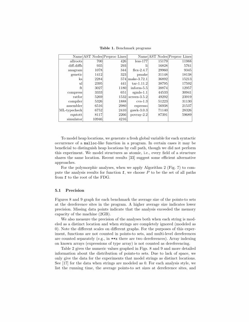
Table 1. Benchmark programs

Name AST Nodes Preproc Lines Name AST Nodes Preproc Lines

allroots 700 426 less-177 15179 11988diff.diffh 935 293 li 16828 5761anagram 1078 344 flex-2.4.7 29960 9345

genetic 1412 323 pmake 31148 18138ks 2284 574 make-3.72.1 36892 15213ul 2395 441 tar-1.11.2 38795 17592ft 3027 1180 inform-5.5 38874 12957

compress 3333 651 sgmls-1.1 44533 30941ratfor 5269 1532 screen-3.5.2 49292 23919

compiler 5326 1888 cvs-1.3 51223 31130assembler 6516 2980 espresso 56938 21537

ML-typecheck 6752 2410 gawk-3.0.3 71140 28326eqntott 8117 2266 povray-2.2 87391 59689

simulator 10946 4216

To model heap locations, we generate a fresh global variable for each syntacticoccurrence of a malloc-like function in a program. In certain cases it may bebeneficial to distinguish heap locations by call path, though we did not performthis experiment. We model structures as atomic, i.e., every field of a structureshares the same location. Recent results [33] suggest some efficient alternativeapproaches.

For the polymorphic analyses, when we apply Algorithm 2 (Fig. 7) to com-pute the analysis results for function f, we choose P to be the set of all pathsfrom f to the root of the FDG.

5.1 Precision

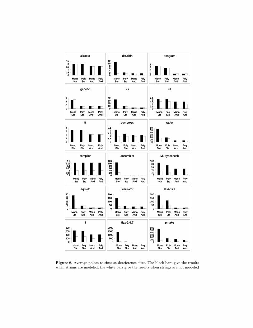
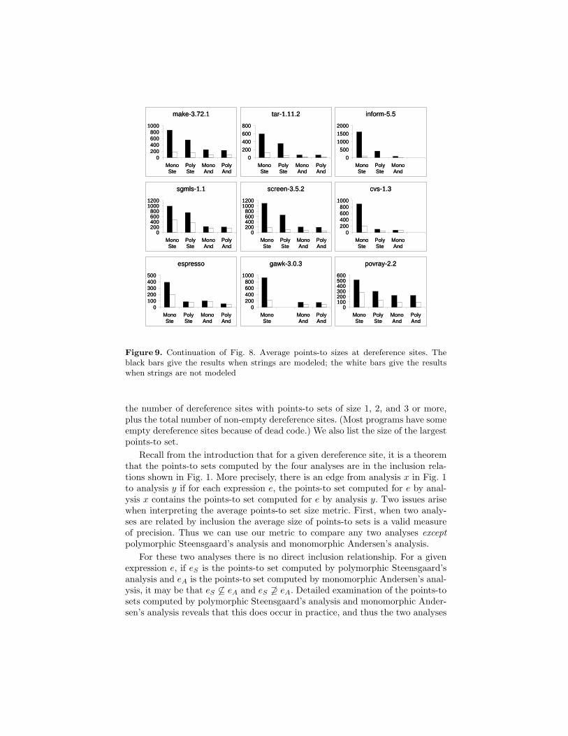
Figures 8 and 9 graph for each benchmark the average size of the points-to setsat the dereference sites in the program. A higher average size indicates lowerprecision. Missing data points indicate that the analysis exceeded the memorycapacity of the machine (2GB).

We also measure the precision of the analyses both when each string is mod-eled as a distinct location and when strings are completely ignored (modeled as0). Note the different scales on different graphs. For the purposes of this exper-iment, functions are not counted in points-to sets, and multi-level dereferencesare counted separately (e.g., in **x there are two dereferences). Array indexingon known arrays (expressions of type array) is not counted as dereferencing.

Table 2 gives the numeric values graphed in Figs. 8 and 9 and more detailedinformation about the distribution of points-to sets. Due to lack of space, weonly give the data for the experiments that model strings as distinct locations.See [17] for the data when strings are modeled as 0. For each analysis style, welist the running time, the average points-to set sizes at dereference sites, and

allroots

00.5

11.5

22.5

MonoSte

PolySte

MonoAnd

PolyAnd

diff.diffh

02468

1012

MonoSte

PolySte

MonoAnd

PolyAnd

anagram

02468

MonoSte

PolySte

MonoAnd

PolyAnd

genetic

0

2

4

6

MonoSte

PolySte

MonoAnd

PolyAnd

ks

010203040

MonoSte

PolySte

MonoAnd

PolyAnd

ul

00.5

11.5

22.5

MonoSte

PolySte

MonoAnd

PolyAnd

ft

0

1

2

3

4

MonoSte

PolySte

MonoAnd

PolyAnd

compress

00.5

11.5

22.5

MonoSte

PolySte

MonoAnd

PolyAnd

ratfor

0102030405060

MonoSte

PolySte

MonoAnd

PolyAnd

compiler

0.90.95

11.051.1

1.151.2

MonoSte

PolySte

MonoAnd

PolyAnd

assembler

020406080

100120

MonoSte

PolySte

MonoAnd

PolyAnd

ML-typecheck

020406080

100

MonoSte

PolySte

MonoAnd

PolyAnd

eqntott

05

1015202530

MonoSte

PolySte

MonoAnd

PolyAnd

simulator

0

50

100

150

200

MonoSte

PolySte

MonoAnd

PolyAnd

less-177

0

50

100

150

200

MonoSte

PolySte

MonoAnd

PolyAnd

li

0

200

400

600

800

MonoSte

PolySte

MonoAnd

PolyAnd

flex-2.4.7

0

500

1000

1500

2000

MonoSte

PolySte

MonoAnd

PolyAnd

pmake

0100200300400500600

MonoSte

PolySte

MonoAnd

PolyAnd

Figure 8. Average points-to sizes at dereference sites. The black bars give the resultswhen strings are modeled; the white bars give the results when strings are not modeled

make-3.72.1

0200400600800

1000

MonoSte

PolySte

MonoAnd

PolyAnd

tar-1.11.2

0

200

400

600

800

MonoSte

PolySte

MonoAnd

PolyAnd

inform-5.5

0

500

1000

1500

2000

MonoSte

PolySte

MonoAnd

sgmls-1.1

0200400600800

10001200

MonoSte

PolySte

MonoAnd

PolyAnd

screen-3.5.2

0200400600800

10001200

MonoSte

PolySte

MonoAnd

PolyAnd

cvs-1.3

0200400600800

1000

MonoSte

PolySte

MonoAnd

espresso

0100200300400500

MonoSte

PolySte

MonoAnd

PolyAnd

gawk-3.0.3

0200400600800

1000

MonoSte

MonoAnd

PolyAnd

povray-2.2

0100200300400500600

MonoSte

PolySte

MonoAnd

PolyAnd

Figure 9. Continuation of Fig. 8. Average points-to sizes at dereference sites. Theblack bars give the results when strings are modeled; the white bars give the resultswhen strings are not modeled

the number of dereference sites with points-to sets of size 1, 2, and 3 or more,plus the total number of non-empty dereference sites. (Most programs have someempty dereference sites because of dead code.) We also list the size of the largestpoints-to set.

Recall from the introduction that for a given dereference site, it is a theoremthat the points-to sets computed by the four analyses are in the inclusion rela-tions shown in Fig. 1. More precisely, there is an edge from analysis x in Fig. 1to analysis y if for each expression e, the points-to set computed for e by anal-ysis x contains the points-to set computed for e by analysis y. Two issues arisewhen interpreting the average points-to set size metric. First, when two analy-ses are related by inclusion the average size of points-to sets is a valid measureof precision. Thus we can use our metric to compare any two analyses exceptpolymorphic Steensgaard’s analysis and monomorphic Andersen’s analysis.

For these two analyses there is no direct inclusion relationship. For a givenexpression e, if eS is the points-to set computed by polymorphic Steensgaard’sanalysis and eA is the points-to set computed by monomorphic Andersen’s anal-ysis, it may be that eS 6⊆ eA and eS 6⊇ eA. Detailed examination of the points-tosets computed by polymorphic Steensgaard’s analysis and monomorphic Ander-sen’s analysis reveals that this does occur in practice, and thus the two analyses

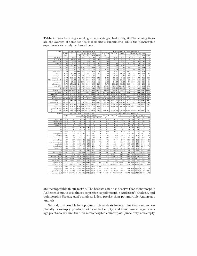
Table 2. Data for string modeling experiments graphed in Fig. 8. The running timesare the average of three for the monomorphic experiments, while the polymorphicexperiments were only performed once.

Name Monomorphic Steensgaard’s Polymorphic Steensgaard’sTime Av. Num. deref sites Up Tm Dn Tm Av. Num. deref sites(s) 1 2 3+ tot max (s) (s) 1 2 3+ tot max

allroots 0.17 2.00 0 42 0 42 2 0.27 0.29 2.00 0 42 0 42 2diff.diffh 0.23 11.25 12 1 23 36 17 0.29 0.55 2.36 14 13 9 36 5anagram 0.25 6.74 11 1 30 42 9 0.37 1.00 5.45 12 0 30 42 8

genetic 0.36 4.95 22 8 46 76 15 0.45 1.18 1.43 62 10 4 76 10ks 0.43 33.83 3 13 99 115 39 0.53 1.38 8.86 3 13 99 115 10ul 0.49 2.22 55 129 54 238 4 0.59 2.97 2.16 55 137 46 238 4ft 0.65 3.39 29 8 133 170 4 1.05 4.58 3.35 37 0 133 170 4

compress 0.73 2.13 181 44 36 261 8 0.94 5.32 1.44 181 44 36 261 3ratfor 1.65 53.41 36 4 125 165 80 2.71 30.90 18.65 36 7 122 165 62

compiler 1.15 1.17 65 13 0 78 2 2.47 5.76 1.17 65 13 0 78 2assembler 2.54 108.03 79 31 273 383 213 5.22 58.96 2.98 223 36 124 383 120

ML-typecheck 2.92 88.41 28 0 285 313 97 3.92 60.87 70.33 28 27 258 313 85eqntott 2.70 27.82 68 110 436 614 42 3.45 54.17 6.17 76 133 405 614 11

simulator 3.78 150.11 24 13 259 296 223 5.70 118.20 33.71 105 5 186 296 89less-177 5.66 185.55 69 13 490 572 219 18.28 321.89 114.13 80 14 478 572 173

li 18.67 643.88 8 0 933 941 657 33.33 695.71 629.01 8 0 933 941 644flex-2.4.7 64.33 1431.68 13 0 1613 1626 1445 22.09 818.25 43.83 15 2 1609 1626 1226

pmake 20.98 556.19 40 2 2501 2543 570 373.97 4416.16 151.69 100 9 2434 2543 218make-3.72.1 40.05 863.25 90 222 3170 3482 975 265.43 1045.70 556.94 311 158 3013 3482 666

tar-1.11.2 26.10 597.13 87 70 2031 2188 656 23.16 776.65 356.20 183 114 1888 2185 434inform-5.5 47.81 1618.62 21 0 1268 1289 1648 2601.61 67608.52 408.47 28 0 1261 1289 601sgmls-1.1 69.70 987.71 96 11 2382 2489 1046 126.08 3961.22 749.20 123 15 2351 2489 867

screen-3.5.2 64.79 1093.00 27 9 4915 4951 1110 65.37 1991.28 656.86 112 36 4803 4951 768cvs-1.3 47.42 894.44 97 680 2276 3053 1242 124.80 2949.33 100.18 1159 141 1753 3053 367

espresso 34.40 391.59 101 530 5479 6110 456 104.65 3368.75 86.78 1238 595 4277 6110 171gawk-3.0.3 78.30 927.57 139 50 4930 5119 966 — — — — — — — —povray-2.2 64.72 515.85 761 407 8044 9212 618 111.38 6606.45 299.41 1027 659 7526 9212 434

Name Monomorphic Andersen’s Polymorphic Andersen’sTime Av. Num. deref sites Up Tm Dn Tm Av. Num. deref sites(s) 1 2 3+ tot max (s) (s) 1 2 3+ tot max

allroots 0.18 1.57 18 24 0 42 2 0.14 0.22 1.57 18 24 0 42 2diff.diffh 0.18 1.56 25 2 9 36 3 0.21 0.49 1.56 25 2 9 36 3anagram 0.24 1.10 38 4 0 42 2 0.16 0.72 1.10 38 4 0 42 2

genetic 0.22 1.43 62 10 4 76 10 0.21 0.76 1.43 62 10 4 76 10ks 0.37 3.58 9 22 84 115 5 0.33 0.98 3.58 9 22 84 115 5ul 0.24 1.61 184 8 46 238 4 0.23 0.91 1.61 184 8 46 238 4ft 0.42 2.12 75 0 95 170 3 0.56 2.25 2.12 75 0 95 170 3

compress 0.34 1.18 215 46 0 261 2 0.41 1.42 1.18 215 46 0 261 2ratfor 0.63 6.27 56 9 100 165 47 1.22 5.99 6.27 56 9 100 165 47

compiler 0.57 1.17 65 13 0 78 2 0.96 5.07 1.17 65 13 0 78 2assembler 1.07 2.87 225 36 122 383 120 3.02 80.46 2.87 225 36 122 383 120

ML-typecheck 0.99 45.87 101 30 182 313 78 1.79 14.81 45.87 101 30 182 313 78eqntott 1.03 1.92 239 199 176 614 5 1.50 11.20 1.92 239 199 176 614 5

simulator 1.35 28.53 107 10 179 296 72 2.32 51.70 27.78 107 10 179 296 71less-177 2.55 12.98 221 92 259 572 110 4.35 184.03 12.72 238 101 233 572 110

li 4.44 421.23 28 0 913 941 465 189.49 9929.88 421.23 28 0 913 941 465flex-2.4.7 4.81 6.22 734 204 688 1626 1226 8.61 173.97 6.21 735 204 687 1626 1226

pmake 5.11 129.16 401 98 2044 2543 175 21.38 682.71 88.64 452 98 1993 2543 144make-3.72.1 9.02 250.85 619 268 2595 3482 494 13.18 390.35 230.12 652 264 2566 3482 487

tar-1.11.2 6.89 69.07 330 741 1117 2188 200 7.74 327.48 66.11 336 742 1107 2185 194inform-5.5 6.95 80.51 657 20 612 1289 227 — — — — — — — —sgmls-1.1 8.14 224.11 687 321 1481 2489 506 40.52 1121.89 205.63 703 323 1463 2489 492

screen-3.5.2 7.45 206.48 339 39 4573 4951 241 1277.15 2028.85 195.83 342 44 4565 4951 232cvs-1.3 10.82 71.27 1281 192 1580 3053 203 — — — — — — — —

espresso 12.89 101.21 1824 300 3986 6110 175 28.81 967.64 56.34 1973 304 3833 6110 152gawk-3.0.3 12.40 157.28 1177 226 3716 5119 237 22.14 763.62 148.77 1184 228 3707 5119 225povray-2.2 22.40 223.61 2474 588 6150 9212 402 169.51 5574.82 223.61 2474 588 6150 9212 402

are incomparable in our metric. The best we can do is observe that monomorphicAndersen’s analysis is almost as precise as polymorphic Andersen’s analysis, andpolymorphic Steensgaard’s analysis is less precise than polymorphic Andersen’sanalysis.

Second, it is possible for a polymorphic analysis to determine that a monomor-phically non-empty points-to set is in fact empty, and thus have a larger aver-age points-to set size than its monomorphic counterpart (since only non-empty

points-to sets are included in this average). However, we can eliminate this pos-sibility by counting the total number of nonempty dereference sites. (A polymor-phic analysis cannot have more nonempty dereference sites than its monomor-phic counterpart.) The data in Table 2 shows that for all benchmarks excepttar-1.11.2, the total number of non-empty dereference sites is the same acrossall analyses, and the difference between the polymorphic and monomorphic anal-yses for tar-1.11.2 is miniscule. Therefore we know that averaging the sizes ofnon-empty dereference sites is a valid measure of precision.

5.2 Speed

Table 2 also lists the running times for the analyses. The running times includethe time to compute the least model of the Px variables, i.e., to find the points-tosets. For the polymorphic analyses, we separate the running times into the timefor the bottom-up pass and the time for the top-down pass.

For purposes of this experiment, whose goal is to compare the precision ofmonomorphic and polymorphic points-to analysis, the running times are largelyirrelevant. Thus we have made little effort to make the analyses efficient, andthe running times should all be taken with a grain of salt.

5.3 Discussion

The data presented in Figs. 8 and 9 and Table 2 shows two striking and consistentresults:

1. Polymorphic Andersen’s analysis is hardly more precise than monomorphicAndersen’s analysis.

2. Polymorphic Steensgaard’s analysis is much more precise than monomorphicSteensgaard’s analysis.

The only exceptions to these trends are some of the smaller programs (all-roots, ul, ft, compiler, li), for which polymorphic Steensgaard’s analysis isnot much more precise than monomorphic Steensgaard’s analysis, and one largerprogram, espresso, for which Polymorphic Andersen’s analysis is noticeablymore precise than Monomorphic Andersen’s analysis. Additionally, notice thatfor all programs except espresso, polymorphic Steensgaard’s analysis has ahigher average points-to set size than monomorphic Andersen’s analysis. (Recallthat this does not necessarily imply strictly increased precision.)

To understand these results, consider the following code skeleton:

void f() { ... h(a); ... }void g() { ... h(b); ... }void h(int *c) { ... }

In Steensgaard’s equality-based monomorphic analysis, the types of all argu-ments for all calls sites of a function are equated. In the example, this resultsin a = b = c, where a is a’s points-to type, b is b’s points-to type, and c is c’s

Table 3. Potential polymorphism. The measurements include library functions.

Name Call Sites % Void Name Call Sites % Void

allroots 55 69 less-177 1091 56

diff.diffh 67 58 li 1243 37

anagram 59 75 flex-2.4.7 1205 79

genetic 79 75 pmake 1943 56

ks 101 84 make-3.72.1 1955 50

ul 103 74 tar-1.11.2 1586 54

ft 152 70 inform-5.5 2593 72

compress 138 73 sgmls-1.1 1614 62

ratfor 306 75 screen-3.5.2 2632 75

compiler 448 89 cvs-1.3 3036 55

assembler 519 66 espresso 2729 51

ML-typecheck 430 31 gawk-3.0.3 2358 51

eqntott 364 61 povray-2.2 3123 59

simulator 677 75

points-to type. In the polymorphic version of Steensgaard’s analysis, a and bcan be distinct. Our measurements show that separating function parameters isimportant for points-to analysis.

In contrast, in Andersen’s monomorphic inclusion-based system, the points-to types of arguments at call sites are potentially separated. In the example, wehave a ⊆ c and b ⊆ c. However, function results are all conflated (i.e., every callsite has the same result, the union of points-to results over all call sites). The factthat polymorphic Andersen’s analysis is hardly more precise than monomorphicAndersen’s analysis suggests that separating function parameters is by far themost important form of polymorphism present in points-to analysis for C.

Thus, we conclude that polymorphism for points-to analysis is useful pri-marily for separating inputs, which can be achieved very nearly as well by amonomorphic inclusion-based analysis. This conclusion begs the question: Whyis there so little polymorphism in points-to results available in C? Directly mea-suring the polymorphism available in output side effects of C functions is difficult,although we hypothesize that C functions tend to side-effect global variables andheap data (which our analyses model as global) rather than stack-allocated data.

We can measure the polymorphism of result types fairly directly. Table 3 listsfor each benchmark the number of call sites and percentage of calls that occurin void contexts. These results emphasize that most C functions are called fortheir side effects: for 25 out of 27 benchmarks, at least half of all calls are invoid contexts. Thus, there is a greatly reduced chance that polymorphism canbe beneficial for Andersen’s analysis.

It is worth pointing out that the client for a points-to analysis can also havea significant, and often negative, impact on the polymorphism that actually canbe exploited. In the example above, when computing points-to sets for h’s local

variables we conflate information for all of c’s contexts. This summarizationeffectively removes much of the fine detail about the behavior of h in differentcalling contexts. However, many applications require points-to information thatis valid in every calling context. In addition, if we attempt to distinguish all callpaths, the analysis can quickly become intractable.

6 Conclusion

We have explored two dimensions of the design space for flow-insensitive points-to analysis for C: polymorphic versus monomorphic and inclusion-based versusequality-based. Our experiments show that while polymorphism is potentiallybeneficial for equality-based points-to analysis, it does not have much benefit forinclusion-based points-to analysis. Even though we feel that added engineeringeffort can make the running times of the polymorphic analyses much faster, theprecision would still be the same.

Monomorphic Andersen’s analysis can be made fast [30] and often providesfar more precise results than monomorphic Steensgaard’s analysis. PolymorphicSteensgaard’s analysis is in general much less precise than polymorphic Ander-sen’s analysis, which is in turn little more precise than monomorphic Andersen’sanalysis. Additionally, as discussed in Sect. 4.3, implementing polymorphism isa complicated and difficult task. Thus, we feel that monomorphic Andersen’sanalysis may be the best choice among the four analyses.

Acknowledgements We thank the anonymous referees for their helpful com-ments. We would also like to thank Manuvir Das for suggestions for the imple-mentation.

References

[1] A. Aiken, M. Fahndrich, J. S. Foster, and Z. Su. A Toolkit for ConstructingType- and Constraint-Based Program Analyses. In X. Leroy and A. Ohori, edi-tors, Proceedings of the second International Workshop on Types in Compilation,volume 1473 of Lecture Notes in Computer Science, pages 78–96, Kyoto, Japan,Mar. 1998. Springer-Verlag.

[2] A. Aiken and E. L. Wimmers. Solving Systems of Set Constraints. In Proceedings,Seventh Annual IEEE Symposium on Logic in Computer Science, pages 329–340,Santa Cruz, California, June 1992.

[3] A. Aiken and E. L. Wimmers. Type Inclusion Constraints and Type Inference.In FPCA ’93 Conference on Functional Programming Languages and ComputerArchitecture, pages 31–41, Copenhagen, Denmark, June 1993.

[4] L. O. Andersen. Program Analysis and Specialization for the C ProgrammingLanguage. PhD thesis, DIKU, Department of Computer Science, University ofCopenhagen, May 1994.

[5] M. Burke, P. Carini, J.-D. Choi, and M. Hind. Flow-Insensitive InterproceduralAlias Analysis in the Presence of Pointers. In K. Pingali, U. Banerjee, D. Gelern-ter, A. Nicolau, and D. Padua, editors, Proceedings of the Seventh Workshop on

Languages and Compilers for Parallel Computing, volume 892 of Lecture Notes inComputer Science, pages 234–250. Springer-Verlag, 1994.

[6] R. Chatterjee, B. G. Ryder, and W. A. Landi. Relevant Context Inference. In Pro-ceedings of the 26th Annual ACM SIGPLAN-SIGACT Symposium on Principlesof Programming Languages, pages 133–146, San Antonio, Texas, Jan. 1999.

[7] M. Das. Unification-based Pointer Analysis with Directional Assignments. InProceedings of the 2000 ACM SIGPLAN Conference on Programming LanguageDesign and Implementation, Vancouver B.C., Canada, June 2000. To appear.

[8] S. Debray, R. Muth, and M. Weippert. Alias Analysis of Executable Code. In Pro-ceedings of the 25th Annual ACM SIGPLAN-SIGACT Symposium on Principlesof Programming Languages, pages 12–24, San Diego, California, Jan. 1998.

[9] A. Deutsch. Interprocedural May-Alias Analysis for Pointers: Beyond k-limiting.In Proceedings of the 1994 ACM SIGPLAN Conference on Programming LanguageDesign and Implementation, pages 230–241, Orlando, Florida, June 1994.

[10] N. Dor, M. Rodeh, and M. Sagiv. Detecting Memory Errors via Static PointerAnalysis. In Proceedings of the ACM SIGPLAN/SIGSOFT Workshop on ProgramAnalysis for Software Tools and Engineering, pages 27–34, Montreal, Canada,June 1998.

[11] M. Emami, R. Ghiya, and L. J. Hendren. Context-Sensitive InterproceduralPoints-to Analysis in the Presence of Function Pointers. In Proceedings of the1994 ACM SIGPLAN Conference on Programming Language Design and Imple-mentation, pages 242–256, Orlando, Florida, June 1994.

[12] M. Fahndrich. BANE: A Library for Scalable Constraint-Based Program Analysis.PhD thesis, University of California, Berkeley, 1999.

[13] M. Fahndrich and A. Aiken. Program Analysis using Mixed Term and Set Con-straints. In P. V. Hentenryck, editor, Static Analysis, Fourth International Sym-posium, volume 1302 of Lecture Notes in Computer Science, pages 114–126, Paris,France, Sept. 1997. Springer-Verlag.

[14] M. Fahndrich, J. S. Foster, Z. Su, and A. Aiken. Partial Online Cycle Elimina-tion in Inclusion Constraint Graphs. In Proceedings of the 1998 ACM SIGPLANConference on Programming Language Design and Implementation, pages 85–96,Montreal, Canada, June 1998.

[15] M. Fahndrich, J. Rehof, and M. Das. Scalable Context-Sensitive Flow Analysisusing Instantiation Constraints. In Proceedings of the 2000 ACM SIGPLAN Con-ference on Programming Language Design and Implementation, Vancouver B.C.,Canada, June 2000. To appear.

[16] J. S. Foster, M. Fahndrich, and A. Aiken. Flow-Insensitive Points-to Analysiswith Term and Set Constraints. Technical Report UCB//CSD-97-964, Universityof California, Berkeley, Aug. 1997.

[17] J. S. Foster, M. Fahndrich, and A. Aiken. Polymorphic versus Monomorphic Flow-insensitive Points-to Analysis for C. Technical report, University of California,Berkeley, Apr. 2000.

[18] N. Heintze and J. Jaffar. A Decision Procedure for a Class of Set Constraints. InProceedings, Fifth Annual IEEE Symposium on Logic in Computer Science, pages42–51, Philadelphia, Pennsylvania, June 1990.

[19] M. Hind and A. Pioli. Assessing the Effects of Flow-Sensitivity on Pointer AliasAnalyses. In G. Levi, editor, Static Analysis, Fifth International Symposium,volume 1503 of Lecture Notes in Computer Science, pages 57–81, Pisa, Italy, Sept.1998. Springer-Verlag.

[20] W. Landi and B. G. Ryder. A Safe Approximate Algorithm for InterproceduralPointer Aliasing. In Proceedings of the 1992 ACM SIGPLAN Conference on Pro-gramming Language Design and Implementation, pages 235–248, San Francisco,California, June 1992.

[21] R. Milner. A Theory of Type Polymorphism in Programming. Journal of Com-puter and System Sciences, 17:348–375, 1978.

[22] C. Mossin. Flow Analysis of Typed Higher-Order Programs. PhD thesis, DIKU,Department of Computer Science, University of Copenhagen, 1996.

[23] R. O’Callahan and D. Jackson. Lackwit: A Program Understanding Tool Based onType Inference. In Proceedings of the 19th International Conference on SoftwareEngineering, pages 338–348, Boston, Massachusetts, May 1997.

[24] M. Odersky, M. Sulzmann, and M. Wehr. Type Inference with Constrained Types.In B. Pierce, editor, Proceedings of the 4th International Workshop on Foundationsof Object-Oriented Languages, Jan. 1997.

[25] D. Remy. Typechecking records and variants in a natural extension of ML. In Pro-ceedings of the 16th Annual ACM SIGPLAN-SIGACT Symposium on Principlesof Programming Languages, pages 77–88, Austin, Texas, Jan. 1989.

[26] E. Ruf. Context-Insensitive Alias Analysis Reconsidered. In Proceedings of the1995 ACM SIGPLAN Conference on Programming Language Design and Imple-mentation, pages 13–22, La Jolla, California, June 1995.

[27] M. Sagiv, T. Reps, and R. Wilhelm. Parametric Shape Analysis via 3-ValuedLogic. In Proceedings of the 26th Annual ACM SIGPLAN-SIGACT Symposiumon Principles of Programming Languages, pages 105–118, San Antonio, Texas,Jan. 1999.

[28] M. Shapiro and S. Horwitz. Fast and Accurate Flow-Insensitive Points-To Anal-ysis. In Proceedings of the 24th Annual ACM SIGPLAN-SIGACT Symposium onPrinciples of Programming Languages, pages 1–14, Paris, France, Jan. 1997.

[29] B. Steensgaard. Points-to Analysis in Almost Linear Time. In Proceedings of the23rd Annual ACM SIGPLAN-SIGACT Symposium on Principles of ProgrammingLanguages, pages 32–41, St. Petersburg Beach, Florida, Jan. 1996.

[30] Z. Su, M. Fahndrich, and A. Aiken. Projection Merging: Reducing Redun-dancies in Inclusion Constraint Graphs. In Proceedings of the 27th AnnualACM SIGPLAN-SIGACT Symposium on Principles of Programming Languages,Boston, Massachusetts, Jan. 2000. To appear.

[31] R. P. Wilson and M. S. Lam. Efficient Context-Sensitive Pointer Analysis for CPrograms. In Proceedings of the 1995 ACM SIGPLAN Conference on Program-ming Language Design and Implementation, pages 1–12, La Jolla, California, June1995.

[32] A. K. Wright. Simple Imperative Polymorphism. In Lisp and Symbolic Compu-tation 8, volume 4, pages 343–356, 1995.

[33] S. H. Yong, S. Horwitz, and T. Reps. Pointer Analysis for Programs with Struc-tures and Casting. In Proceedings of the 1999 ACM SIGPLAN Conference on Pro-gramming Language Design and Implementation, pages 91–103, Atlanta, Georgia,May 1999.

[34] S. Zhang, B. G. Ryder, and W. A. Landi. Program Decomposition for PointerAliasing: A Step toward Practical Analyses. In Fourth Symposium on the Foun-dations of Software Engineering, Oct. 1996.

[35] S. Zhang, B. G. Ryder, and W. A. Landi. Experiments with Combined Analysisfor Pointer Aliasing. In Proceedings of the ACM SIGPLAN/SIGSOFT Workshopon Program Analysis for Software Tools and Engineering, pages 11–18, Montreal,Canada, June 1998.