Institute for International Economic Policy Working Paper Series Elliott School of International Affairs The George Washington University

Pollution or Crime: The Effect of Driving Restrictions on Criminal Activity

IIEP-WP-2016-31

Paul E. Carrillo

George Washington University

Andrea Lopez George Washington University

Arun Malik

George Washington University

May 2016 Institute for International Economic Policy 1957 E St. NW, Suite 502 Voice: (202) 994-5320 Fax: (202) 994-5477 Email: iiep@gwu.edu Web: www.gwu.edu/~iiep

Pollution or Crime:The Effect of Driving Restrictions on Criminal Activity∗

Paul E. Carrillo†

Andrea Lopez‡

Arun Malik§

May 2016

Abstract

Driving restriction programs have been implemented in many cities around theworld to alleviate pollution and congestion problems. Enforcement of such programsis costly and can potentially displace policing resources used for crime prevention andcrime detection. Hence, driving restrictions may increase crime. To test this hypoth-esis, we exploit both temporal and spatial variation in the implementation of Quito,Ecuador’s Pico y Placa program, and evaluate its effect on crime. Both difference-in-difference and spatial regression discontinuity estimates provide credible evidence thatdriving restrictions can increase crime rates.

Keywords: Crime, Difference-in-Differences, Regression Discontinuity, Crime displace-mentJEL Codes: C20, Q52, R28, R48

∗We would like to thank Antonio Bento, Samuel Berlinski, Laura Jaitman, Carlos Scartascini, Anthony Yezer, and partici-pants at the 2015 ASSA-AREUEA Conference, the Inter-American Bank Research Department seminar, the George WashingtonUniversity Applied Micro Workshop, and Flacso-Ecuador seminar for comments and useful discussions. We are also grateful tothe staff of the Observatorio Metropolitano de Seguridad Ciudadana and Centro de Estudios Fiscales for outstanding collabo-ration. This document is also available at the Inter-American Development Bank’s (IADB) website (IADB Working Paper No.698). Paul Carrillo would like to acknowledge research support from the IADB. The views expressed in this paper are entirelyours, and no endorsement by the Inter-American Development Bank, its Board of Executive Directors, or the countries theyrepresent is expressed or implied.†George Washington University and Inter-American Development Bank, pcarrill@gwu.edu.‡George Washington University, aflopez@gwu.edu.§George Washington University, amalik@gwu.edu.

1

1 Introduction

Many cities in Latin America, Asia and Europe have imposed restrictions on the use of motor

vehicles in an effort to reduce traffic congestion or improve air quality. The restrictions limit

use of vehicles in either all or part of a city for part of the day.1 The various programs differ

in terms of the types of vehicles that are targeted, the size of the restricted zone, and the

times of day during which restrictions are in effect, but they share common goals of either

reducing traffic congestion or improving air quality, or both.

A handful of studies have examined the effectiveness of these programs, focusing pri-

marily on their ability to improve air quality. Mexico City’s program has received the most

attention,2 but recent papers also examine the programs in Sao Paolo, Bogota, Beijing, Tian-

jin, Santiago and Quito.3 Most studies in the literature conclude that permanent driving

restrictions have not reduced traffic congestion or air pollution. Where reductions have been

detected, they have been short-lived, lasting less than a year. The exception are the studies

of Beijing and Quito’s programs, where noticeable improvements in air quality are attributed

to the implementation of driving restrictions. Viard and Fu (2015) find that every-other-day

driving restrictions in Beijing can decrease pollution levels by as much as 19%; Carrillo et al.

(2015) show that Quito’s driving restriction program, which restricts vehicles one day a week

during peak hours, reduces carbon monoxide levels by almost 10%. The “success” of Quito’s

program is attributed, to a large extent, to its strict enforcement.

In this paper we identify a side-effect of driving restrictions that has yet to be studied:

1The best known is Mexico City’s Hoy No Circula (HNC) program introduced in 1989 to improve airquality. Sao Paulo (Brazil) and Bogota (Colombia) introduced similar programs in 1996 and 1998, respec-tively. Beijing and Tianjin (China) introduced temporary driving restrictions during the 2008 OlympicGames. Athens (Greece) introduced permanent driving restrictions in 1982. Santiago (Chile) has used acombination of permanent and temporary driving restrictions since 1998 to reduce air pollution. Most re-cently, in 2015, Paris and several cities in Italy introduced temporary driving restrictions in response to poorair quality.

2See for example, Eskeland and Feyzioglu (1997), Davis (2008), and Gallego et al. (2013).3Lin et al. (2011), Chen et al. (2011), de Grange and Troncoso (2011), Troncoso et al. (2012) and Bonilla

(2011).

2

Driving restrictions may increase crime rates.4 It is clear that driving restrictions can have a

direct impact on congestion and pollution, but, why would they affect criminal activity? The

crime-and-punishment literature suggests at least two reasons. First, enforcement of driving

restrictions is a resource-intensive endeavor that is typically the responsibility of the police.

The marginal cost of committing a crime depends on the frequency with which criminal

activities are detected. When driving restrictions are imposed, the burden of enforcement

could result in fewer policing resources being allocated to crime prevention. As crime pre-

vention decreases, so does the marginal cost of crime.5 Second, the cost of committing a

crime also depends on the availability of opportunities to engage in criminal activities. If a

driving restriction policy is successfully enforced, it can increase pedestrian flows and public

transportation use, raising the number of potential victims. In equilibrium, a decrease in

the marginal cost of committing a crime would result in higher crime rates.

To test these hypotheses we evaluate the effects of Quito’s Pico y Placa program on

crime. Pico y Placa (PyP) went into effect in Quito on May 3, 2010. It restricts access to

the central part of the city. The last digit of a vehicle’s license plate number determines

the one day of the week on which the vehicle is barred from the road. The PyP program is

well suited to being studied because of the availability of data on criminal offenses for the

parts of the city that are subject to PyP restrictions as well as those that are not. Moreover,

the program restricts vehicles during workday rush (or peak) hours but not weekends or

holidays. These features of the program are exploited to identify treatment effects.

Crime data were gathered from two sources. The first is the Ecuadorian National Police.

We obtain records of every crime reported to the police between January 2010 and May 2012

in Quito and Guayaquil, the two largest urban areas of the country. Our second source of

data is Quito’s Municipal Government (“Observatorio Municipal Ciudadano OMS). OMS

4Davis (2008) is the only study we are aware of that briefly mentions this possibility.5DiTella and Schargrodsky (2004) and Draca et al. (2011) offer evidence that police presence reduces

crime.

3

collects crime data from the police and creates monthly reports on citizen security. They

shared all of their property crime records for the period 2008-2012. Each of these two data

source has advantages and weaknesses. The police data is for all crimes reported to the

police. This data has information on the time of each crime, but it does not have geocoded

information on location of the crimes. The police data are used to calculate the number of

crimes of all types that took place every hour in Quito and in Guayaquil. The OMS data

from Quito’s municipality is a subset of the police records with geocoded information on the

location of crimes. Unfortunately, OMS data are not comparable across time. Their sample

selection criteria changed in April 2009 and reverted back a year later.

Police crime data and a difference-in-difference (DD) strategy are used to assess whether

crime rates during the hours when PyP is in effect changed after the introduction of the

program. In all specifications, the treatment group is working-day peak hours in Quito.

Finding an appropriate control group is not straightforward. Ideally, one would want a

control group that, in the absence of treatment, has the same trend as the treatment group.

Rather than making an ad hoc choice, we use three alternative control groups, each of which

can be a reasonable representation of the counterfactual trend, under appropriate conditions.

The control groups are: a) non-working-day peak hours in Quito, b) working-day off-peak

hours in Quito, and c) working-day peak hours in Guayaquil. Our regression models include

a comprehensive set of controls, including month-year fixed effects, day-hour fixed effects

obtained by interacting each hour of the day with each working day, and a long list of

weather variables. Results show that crime rates in Quito increased during peak hours after

the introduction of PyP relative to changes in each of the control groups. The magnitude of

the effects is large, between 5% and 10%, and statistically significant at conventional levels.

Estimates from our preferred specification suggest that PyP led to an increase of about 0.4

crimes per hour (about 10%) during the restricted hours. Models are also estimated with

several “placebo” samples and no statistically significant results are found.

4

OMS data are used to analyze changes in the spatial distribution of crimes before and

after PyP was introduced. We focus on the spatial distribution of crimes near the boundary

of the restricted zone. The portion of the boundary that passes through populated areas is

demarcated by major roads. Policing resources on these roads, and adjacent areas, are likely

to have been diverted to staff a small number of PyP checkpoints located on the boundary.

Thus, intensity of PyP enforcement and the potential for displacement of policing resources

is likely higher along the boundary. We show that the post-treatment frequency of crimes

as a function of the distance to the boundary has a large spike, or “excess bunching,” at

the boundary. The estimate of excess bunching is large: about 1.6 crimes per meter, over

60% higher than the baseline predicted by a counterfactual without excess bunching. More

importantly, we show that in the pre-treatment period, there is very little excess bunching

at the boundary.6

Excess bunching is much higher in areas just inside the boundary compared to areas

just outside. Even though the displacement of policing resources likely affects both sides

of the boundary, driving restrictions can dispropoportionately affect economic activity and

pedestrian flows inside the restricted zone. For these reason, we also employ a spatial re-

gression discontinuity design to assess if crime rates change discontinuously at the boundary.

Intuitively, crime rates just inside the boundary are compared to their counterparts just out-

side. While in a comparable pre-treatment period the spatial distribution of crime is smooth

around the driving restriction boundary, there is a sharp spike just inside the restricted

zone in the post-treatment sample. Our preferred model’s estimates suggest that PyP has

increased the number of crimes along the inside edge of the boundary by as much as 100%

compared to crime rates on the outside edge.

The combined empirical findings provide credible evidence that PyP has increased crime

rates in Quito during peak hours and near the driving restriction boundary. Do these in-

6The difference between post and pre-treatment excess bunching is 1.39 crimes per meter.

5

creased crime rates reflect a shift in police enforcement allocation or an increase in the use

of public transportation and pedestrian flows, or both? We report evidence of a substantial

commitment of police resources to PyP. As a result, driving restrictions enforcement has

been vigorous: tens of thousands of violations were punished during the first year of the

program alone. On the other hand, we find little evidence that pedestrian flows or public

transportation use has increased. PyP may induce drivers to use alternative forms of trans-

portation, such as walking or public transportation, during the days when they are subject

to the driving restriction, and make them more vulnerable to criminal activities. But we

find no evidence that a crime is more likely to occur on a day when the use of one of the

victim’s vehicles is restricted.

This paper is closely related to studies that analyze the relationship between shifts in

monitoring resources and crime displacement. For example, trade-offs in the allocation

of police resources have been discussed in Benson et al. (1998), Benson et al. (1992) and

Benson and Rasmussen (1991); Yang (2008) also shows evidence of crime displacement in

the contexts of a customs reform; Carrillo et al. (2014) find that an increase of monitoring

efforts on one specific margin of a firm’s tax return can shift misreporting to other margins.

Ours is the first study to document that driving restrictions can increase crime rates.

The rest of this paper is organized as follows. The next section provides a simple con-

ceptual framework. Section 3 describes Quito’s PyP program. Section 4 describes the data

and identification strategy. In Section 5, we discuss our empirical results. The last section

concludes.

2 Conceptual Framework

In this section we present a very simple theoretical model that allows us to illustrate the

channels through which driving restrictions can affect criminal activity. The seminal work of

6

Becker (1968) provides a natural framework to model criminal behavior and to understand

the potential links between driving restrictions and crime.

In our stylized model, a representative criminal devotes a fixed amount of time T to

criminal activity each day, and allocates this time between two mutually exclusive periods

j = {0, 1}. The periods correspond to peak hours (j = 1) and non-peak hours (j = 0), so

that t1 + t0 = T . The total time devoted to daily criminal activities T is exogenous, but

the criminal chooses the optimal intra-day allocation of his time. Alternatively, we can view

the criminal as choosing to allocate his time over space, with j = 1 denoting an area inside

the restricted zone and j = 0 denoting an area outside it. This simplified setup allows us to

focus on the within-day (or within-region) distribution of crime and is consistent with the

setup of the empirical models in subsequent sections. For the sake of brevity and clarity,

the presentation below assumes an intra-day allocation of time. We note, however, that the

model will also serve as a guide to explaining the optimal time allocated to criminal activity

in the areas just inside and outside the restricted zone.

The production of crime, measured by the number of (successful) crimes in a period,

depends on the time allocated to that period and on the number of potential victims νj.

Formally, we let N(tj, νj) be the number of crimes produced during period j and assume that

this function is concave and increasing in each argument (N1 > 0, N2 > 0, N11 < 0, N22 < 0).

Furthermore, we assume that a larger number of victims increases the marginal product of

time devoted to crime (N12 > 0). To keep our exposition simple, we let N(tj, νj) ≡ n(tj)νj ,

with n′ > 0 and n′′ < 0.

Crime costs are a function of the expected value of punishment, and depend on the prob-

ability of detection, arrest and conviction, as well as on penalties (fines and imprisonment).

Without loss of generality, we normalize the penalty to one, and we define θj as the joint

probability of detection, arrest and conviction. Let g denote the average gain from a crime

and assume that g > θj .

7

A risk-neutral criminal’s problem is

maxt0,t1

E[π] = (g − θ0) ∗ n(t0)ν0 + (g − θ1) ∗ n(t1)ν1

subject to the constraint t0 + t1 = T . First-order conditions imply that

(g − θ0) ∗ n′(t∗0)ν0 = (g − θ1) ∗ n′(t∗1)ν1. (1)

Given the concavity of n′(.) it is easy to see that, ceteris paribus, the time allocated for

criminal activities during peak hours increases with ν1; similarly, t∗1 increases as θ1 dimin-

ishes.7 As t∗1 increases, so does the number of crimes during peak hours.

How do driving restrictions affect the intra-day or the intra-regional distribution of crime?

Let us assume that a driving restriction during peak-times is imposed. As is the case in

Quito, Mexico D.F. and many other cities, the enforcement of driving restrictions is typically

the responsibility of the police. Enforcement is a resource-intensive endeavor. Police have

to invest resources both to monitor compliance and to impose penalties. The burden of

enforcement could displace resources and result in fewer policing resources being allocated

to crime prevention, at least in the short run. As we pointed out in the introduction, the

literature has documented trade-offs in the allocation of police resources (Benson et al., 1998,

1992; Benson and Rasmussen, 1991), and provided evidence of crime displacement due to

changes in enforcement (Yang, 2008). In the context of our paper, the shift in enforcement

allocation due to the driving restriction decreases θ1, causing crime rates to rise. If a driving

7Rearranging the optimality condition we obtain that t∗1 solves:

h(t∗1) ≡ n′(T − t∗1)

n′(t∗1)=

(g − θ1) ∗ ν1(g − θ0) ∗ ν0

.

The concavity assumption ensures that n′(.) is decreasing; hence, h(.) is an increasing function. Assumethat an interior solution exists. An increase (decrease) in ν1 (θ1) shifts the right hand side of the equationup, leading to a higher level of t∗1.

8

restriction policy is successfully enforced, it can also increase pedestrian flows and public

transportation use, raising the number of potential victims. In our simple model, ν1 would

increase, leading to a higher production of crime during peak hours (or in areas inside the

restricted zone).

Thus, driving restrictions could affect crime prevention, pedestrian flows or both, increas-

ing crime rates during restricted hours and/or in areas inside the restricted zone. To test

these implications we evaluate the effects of Quito’s Pico y Placa (PyP) program on crime.

3 Pico y Placa Program

The city of Quito is located in north-central Ecuador. The city is part of the much larger

Metropolitan District of Quito (MDQ), which is shown in Figure 1. The city has an area

of 372 square km and a population of 1.6 million, whereas the MDQ has an area of 4,218

square km and a population of 2.2 million.

PyP restricts the circulation of vehicles in a restricted zone identified by the solid line in

Figure 1. The boundary was carefully chosen and coincides with highly trafficked roads that

skirt the city. Particularly in the north and south west portions of the city, the boundary

crosses areas with high population density and economic activity. The program regulates

access to the city center during non-holiday weekday rush hours, 7:00-9:30am and 4:00-

7:30pm. On weekends and holidays, there are no restrictions. While both private and

government-owned light vehicles (motorcycles, cars, SUVs, and pickup trucks) face PyP

restrictions, heavy vehicles, taxis, and other forms of public transportation are exempt. As

is the case in other cities, vehicle use on particular days is restricted based on the last digit

of each vehicle’s license plate number. For example, as of December 2012, circulation of

vehicles with license plates ending in 1 or 2 (3 or 4) face restrictions on Monday (Tuesday),

etc.

9

The enforcement of PyP began on May 3, 2010, and it has been extended every six

months since its implementation. Unlike other programs, the days associated with particu-

lar license numbers has not changed since PyP’s inception. According to the municipality

(ADMQ, 2010), PyP was designed with several aims in mind: (i) to reduce emissions of

conventional mobile-source pollutants as well as emissions of greenhouse gases, (ii) to reduce

traffic congestion during rush hours, and (iii) to reduce gasoline and diesel fuel consumption

in order to lower government expenditures on subsidies to these fuels. Theoretically, PyP

should reduce the number of vehicles in the restricted categories by up to 20% during rush

hour. Quito’s municipal government predicted a 2.36% reduction in the number of vehicles

on the road each day, and an equal reduction in vehicular emissions (ADMQ, 2010). Car-

rillo et al. (2015) find evidence that PyP led to a reduction of ambient carbon monoxide

concentration (CO) during peak hours of about 9%. Because levels of CO have been shown

to be correlated with traffic flows, Carrillo et al. (2015) conclude that PyP may have also

decreased traffic congestion.

Enforcement of PyP has been the responsibility of both national and municipal police.

Police officers gather in 12 strategic locations near the main access points to the restricted

zone (shown in Figure 1), and 15 additional teams locate in random points inside the city

(Municipio del Distrito Metropolitano de Quito, Secretaria de Movilidad 2012). While the

exact allocation of policing resources is confidential to the police, internal reports confirm

that police presence has been historically strong along many of the streets that form the

boundary, and that after the introduction of PyP, the police allocated its manpower to both

crime prevention and enforcement of the driving restrictions.

Penalties for violating the PyP rules are stiff. For the first violation, cars are impounded

for one day, and for up to five days for three or more violations. Violators must also pay fines,

the amounts of which are linked to Ecuador’s monthly minimum wage. The first violation

requires a payment of one-third of the monthly minimum wage (USD 97 as of 2012), half

10

the monthly wage for the second violation, and the full monthly wage for the third and

subsequent violations (USD 292 as of 2012). According to the municipal government, PyP

has been stringently enforced, with over 55,000 violations punished over the first 13 months

(EMMOP, 2011, 2012). Police resources are also needed to impose the stiff penalties. With

over 200 daily vehicle violations per working day, the manpower needed to handle this number

of impoundments is likely very large.

4 Data and Methods

4.1 Crime Data

Crime data come from two sources. Our first source is the Ecuadorian National Police

(Policıa Nacional del Ecuador.) The National Police allowed us to collect information from

their administrative records. We obtained descriptions of every crime (including property

and other types of crimes) reported between January 1, 2010 and May 31, 2012 in Quito

and Guayaquil, the two largest urban areas in the country. More than 140,000 crimes were

reported over this period. Crime data from previous years were unavailable. Using crime data

from the original source (the police) has several advantages. The data have not been subject

to any type of manipulation, nor have they been aggregated in any way. They include all

information available to police including the date and time of each reported crime.8 Finally,

police administrative records could be used to find certain characteristics of victims, such as

vehicle ownership.9 We use the individual records to calculate the total number of crimes

that took place every hour in Quito and in Guayaquil. We will exploit time variation of

8The identity of the victim was not included. The description of the crime is, unfortunately, not stan-dardized.

9We exploit these features of the data in the last section to assess if individuals are more likely to bevictimized on a day when they face a driving restriction. Even though we obtained the last digit of thelicense plate number of the cars owned by crime victims, the identity of the victim remained anonymous tous.

11

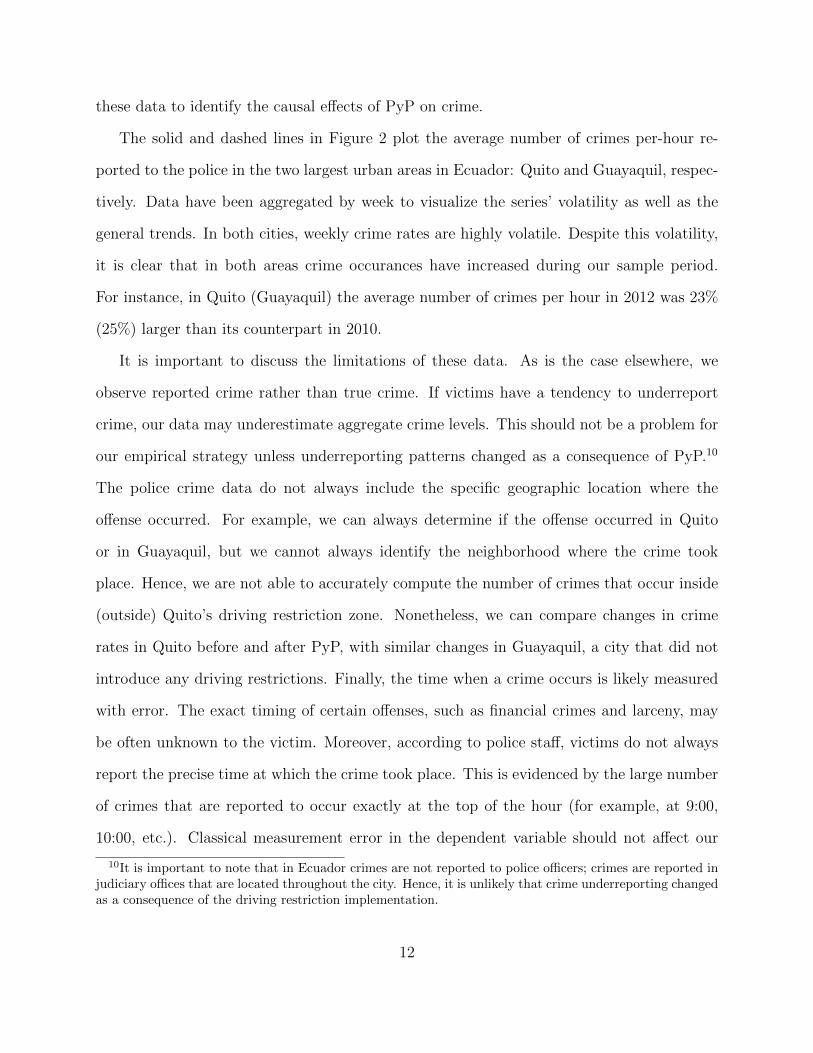
these data to identify the causal effects of PyP on crime.

The solid and dashed lines in Figure 2 plot the average number of crimes per-hour re-

ported to the police in the two largest urban areas in Ecuador: Quito and Guayaquil, respec-

tively. Data have been aggregated by week to visualize the series’ volatility as well as the

general trends. In both cities, weekly crime rates are highly volatile. Despite this volatility,

it is clear that in both areas crime occurances have increased during our sample period.

For instance, in Quito (Guayaquil) the average number of crimes per hour in 2012 was 23%

(25%) larger than its counterpart in 2010.

It is important to discuss the limitations of these data. As is the case elsewhere, we

observe reported crime rather than true crime. If victims have a tendency to underreport

crime, our data may underestimate aggregate crime levels. This should not be a problem for

our empirical strategy unless underreporting patterns changed as a consequence of PyP.10

The police crime data do not always include the specific geographic location where the

offense occurred. For example, we can always determine if the offense occurred in Quito

or in Guayaquil, but we cannot always identify the neighborhood where the crime took

place. Hence, we are not able to accurately compute the number of crimes that occur inside

(outside) Quito’s driving restriction zone. Nonetheless, we can compare changes in crime

rates in Quito before and after PyP, with similar changes in Guayaquil, a city that did not

introduce any driving restrictions. Finally, the time when a crime occurs is likely measured

with error. The exact timing of certain offenses, such as financial crimes and larceny, may

be often unknown to the victim. Moreover, according to police staff, victims do not always

report the precise time at which the crime took place. This is evidenced by the large number

of crimes that are reported to occur exactly at the top of the hour (for example, at 9:00,

10:00, etc.). Classical measurement error in the dependent variable should not affect our

10It is important to note that in Ecuador crimes are not reported to police officers; crimes are reported injudiciary offices that are located throughout the city. Hence, it is unlikely that crime underreporting changedas a consequence of the driving restriction implementation.

12

identification strategy.

Our second source of data is Quito’s Citizen Security Department, the “Observatorio

Metropolitano de Seguridad Ciudadana” (OMS). OMS is part of Quito’s local government,

and it is in charge of monitoring criminal activity in the city. OMS periodically receives

information from the National Police about most types of reported crimes in this city, in-

cluding property crimes, sexual assaults, and homicides. OMS adds geographic references to

each reported crime and produces monthly crime activity reports.11 OMS crime data contain

information about the type of offense, the date on which it occurred and an indicator if it

included an assault. The data provided to us do not contain the exact time (hour) when the

reported crime took place. We collected property crime OMS data for the years 2008, 2009,

2010, 2011 and 2012.

Unfortunately, OMS data are not entirely comparable across time. After March 2009,

certain types of robberies (some non-violent larceny and thefts) were excluded from OMS’s

sample. Hence, the number of crimes recorded by OMS sharply decreased after this date.

This sharp decrease, of course, does not reflect a drop in criminal activity per se, but rather

reflects a change in the way OMS collected its crime statistics. In March 2010, OMS reverted

back to its original criteria and, as a result, reported crime rates climbed significantly. A

discussion of these issues is found in the 2010 OMS Annual Report (OMS, 2010). As a

result, we cannot exploit time variation of these data to identify the effects of PyP on crime.

Instead, we will take advantage of the geographic coordinates to assess if crime rates change

discontinuously at the driving restriction boundary.

It is useful to compare our two data sources. Police data are used to calculate the total

number of crimes that took place every hour in Quito and in Guayaquil. This allows us

to estimate changes in the distribution of crime within the day after the introduction of

11Police crime reports do not have geographic identifiers. They contain long narratives that include theaddress where the crime occurred. OMS looks at these addresses and finds the corresponding geographiccoordinates. Monthly reports are available at http://omsc.quito.gob.ec.

13

PyP. Police data, however, do not contain exact geographic references. The OMS dataset is

basically a subset of the police administrative records that contains geographic references,12

but it does not contain the exact hour when the offense took place and is not comparable

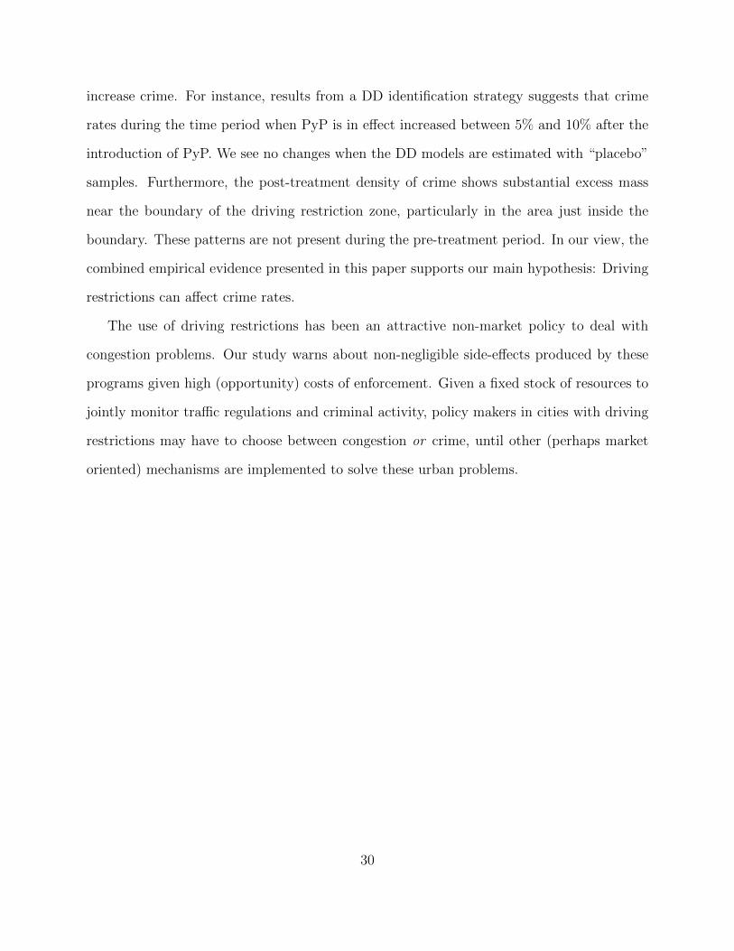
before and after PyP. Figure 3 plots the evolution of total crimes aggregate by month for

the two datasets. As expected, the total number of crimes in the police records is somewhat

higher than in OMS’s, but the trends are fairly similar. Police crime data are used to assess

if the distribution of crime within a day has changed after the introduction of the program.

We use OMS data to assess if crime rates change discontinuously at the driving restriction

boundary after the introduction of PyP.

4.2 Methods

To identify the effect of PyP on crime we use a two-pronged approach. First, we exploit time

variation and employ a difference-in-difference strategy, where we assess if crimes rates during

working day peak hours –the period affected by PyP– has changed after the introduction of

the program relative to three potential control groups. Our second strategy exploits spatial

variation of crime rates. Here we assess if, after PyP was implemented, crime rates change

discontinuously at the driving restriction boundary.

4.2.1 Exploiting Time Variation

To explore the relationship between PyP and crime we use a difference-in-difference (DD)

identification strategy and a series of “placebo” tests. In all empirical models below the

treatment group consists of the period affected by PyP: peak hours of working days in Quito.

The choice of a valid control group, however, is not obvious. The DD strategy requires that, in

the absence of treatment, there should be a common trend for treatment and control groups.

Put differently, the pre-treatment trends of treatment and control should be parallel. Rather

12Some crimes such as financial crimes, or fraud appear in the police data but not in OMS’s.

14

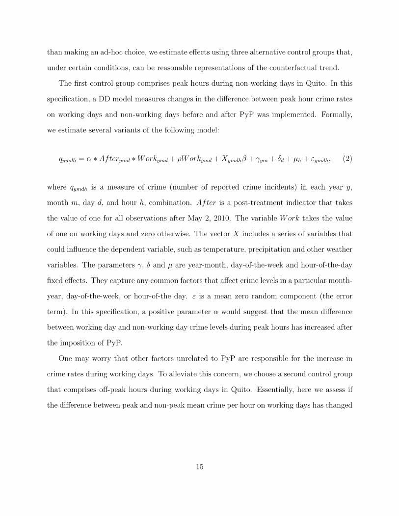
than making an ad-hoc choice, we estimate effects using three alternative control groups that,

under certain conditions, can be reasonable representations of the counterfactual trend.

The first control group comprises peak hours during non-working days in Quito. In this

specification, a DD model measures changes in the difference between peak hour crime rates

on working days and non-working days before and after PyP was implemented. Formally,

we estimate several variants of the following model:

qymdh = α ∗ Afterymd ∗Workymd + ρWorkymd +Xymdhβ + γym + δd + µh + εymdh, (2)

where qymdh is a measure of crime (number of reported crime incidents) in each year y,

month m, day d, and hour h, combination. After is a post-treatment indicator that takes

the value of one for all observations after May 2, 2010. The variable Work takes the value

of one on working days and zero otherwise. The vector X includes a series of variables that

could influence the dependent variable, such as temperature, precipitation and other weather

variables. The parameters γ, δ and µ are year-month, day-of-the-week and hour-of-the-day

fixed effects. They capture any common factors that affect crime levels in a particular month-

year, day-of-the-week, or hour-of-the day. ε is a mean zero random component (the error

term). In this specification, a positive parameter α would suggest that the mean difference

between working day and non-working day crime levels during peak hours has increased after

the imposition of PyP.

One may worry that other factors unrelated to PyP are responsible for the increase in

crime rates during working days. To alleviate this concern, we choose a second control group

that comprises off-peak hours during working days in Quito. Essentially, here we assess if

the difference between peak and non-peak mean crime per hour on working days has changed

15

after the introduction of the policy. Formally, variants of the following model are estimated

qymdh = α ∗ Afterymd ∗ Peakh +Xymdhβ + γym + δd + µh + εymdh, (3)

where the variable Peak takes the value of one for peak hours and zero otherwise. The

parameter α measures the treatment effect: the change in the mean difference between peak

and non-peak crime levels after the imposition of PyP. This DD specification implicitly

assumes that crime trends during non-peak hours are a valid counterfactual trend in the

absence of the program. This is a somewhat strong assumption that may not hold if there

is crime displacement between peak and non-peak hours. Thus, the parameter α should be

interpreted with caution. It certainly measures changes in the distribution of crime within

the day before and after PyP, but it may not be an unbiased estimate of the program’s

treatment effect.

Our third control group consists of working day peak hours in Guayaquil. Guayaquil

is an appealing control for several reasons: a) it is comparable in size to Quito, b) it has

not been subject to driving restrictions, and c) crime displacement between these two cities

is unlikely.13 When Guayaquil is chosen as a control, the DD model tests if the difference

between working day peak hours crime rates in Quito and Guayaquil has increased after the

introduction of PyP. Formally, we estimate several variants of the model

qcymdh = α ∗ Afterymd ∗Quitoc + βQuitoc + γym + δd + µh + εcymdh, (4)

where the subscript c denotes city and the treatment effect is captured by the parameter α.

The general specification of equations (2),(3), and (4) deserves some discussion. To

analyze the determinants of crime, DiTella and Schargrodsky (2004) use a linear model. The

13Travelling costs between these cities are not small: the shortest road trip is over 250 miles and takesabout 7 hours.

16

data used by DiTella and Schargrodsky (2004) is similar in spirit to ours. In their study,

total counts of individuals’ car theft reports are computed in each block-month combination,

and this variable is used as the dependent variable. In our study, we also aggregate crime

reports by location but at a much higher frequency (hourly). Given these similarities, we

choose to follow their approach and employ a linear specification.

As noted, PyP restricts vehicle use in the city of Quito and not elsewhere in Ecuador, and

is in effect only on working day peak hours. We exploit these additional sources of variation

to conduct several “placebo” tests. Specifically, we estimate equations (2), (3), and (4) using

these“placebo” samples and compare estimates with the treatment effects. For instance,

equations (2) and (3) could be estimated with the sample of Guayaquil, and equation (4)

could be estimated using the sample of non-working days. Since all of these samples are not

affected by PyP, finding statistically significant “placebo” effects would call into question

our identification strategy.

4.2.2 Exploiting Spatial Variation

In Section 3 we highlight that: a) enforcement of PyP is limited to areas inside the restriction

zone; b) the restriction boundary coincides with a network of highly trafficked roads; c) police

regularly patrol these boundary roads to monitor crime activity; and d) to enforce driving

restrictions, the police have 12 fixed check points at strategic road intersections near the

boundary. While the actual distribution of policing resources in the city is unknown to us

(and confidential to the police), it is clear that PyP enforcement efforts must have changed

both the level and spatial distribution of crime monitoring activities. Moreover, economic

activity (pedestrian flows) inside the restricted zone may also have been affected by the

introduction of PyP. Hence, to identify the effect of driving restrictions on crime, we also

analyze changes in the spatial distribution of crimes before and after PyP was introduced.

Specifically, a nonparametric estimate of the density of crimes near the boundary is

17

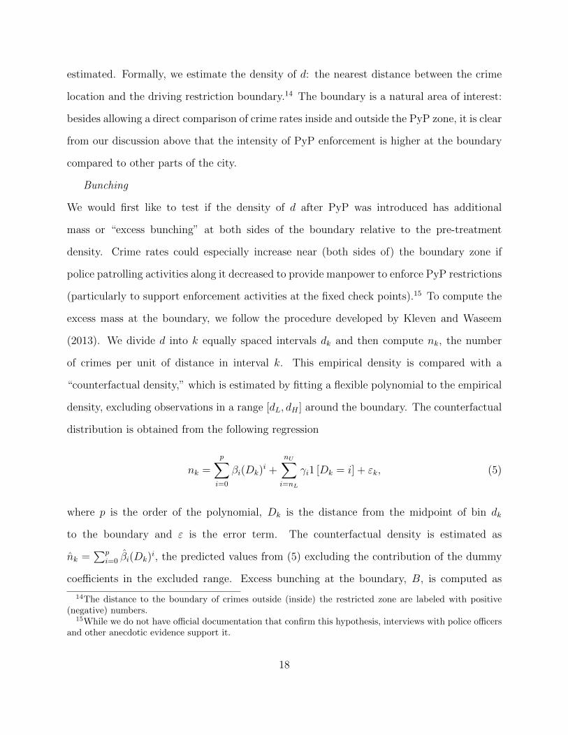
estimated. Formally, we estimate the density of d: the nearest distance between the crime

location and the driving restriction boundary.14 The boundary is a natural area of interest:

besides allowing a direct comparison of crime rates inside and outside the PyP zone, it is clear

from our discussion above that the intensity of PyP enforcement is higher at the boundary

compared to other parts of the city.

Bunching

We would first like to test if the density of d after PyP was introduced has additional

mass or “excess bunching” at both sides of the boundary relative to the pre-treatment

density. Crime rates could especially increase near (both sides of) the boundary zone if

police patrolling activities along it decreased to provide manpower to enforce PyP restrictions

(particularly to support enforcement activities at the fixed check points).15 To compute the

excess mass at the boundary, we follow the procedure developed by Kleven and Waseem

(2013). We divide d into k equally spaced intervals dk and then compute nk, the number

of crimes per unit of distance in interval k. This empirical density is compared with a

“counterfactual density,” which is estimated by fitting a flexible polynomial to the empirical

density, excluding observations in a range [dL, dH ] around the boundary. The counterfactual

distribution is obtained from the following regression

nk =

p∑i=0

βi(Dk)i +

nU∑i=nL

γi1 [Dk = i] + εk, (5)

where p is the order of the polynomial, Dk is the distance from the midpoint of bin dk

to the boundary and ε is the error term. The counterfactual density is estimated as

nk =∑p

i=0 βi(Dk)i, the predicted values from (5) excluding the contribution of the dummy

coefficients in the excluded range. Excess bunching at the boundary, B, is computed as

14The distance to the boundary of crimes outside (inside) the restricted zone are labeled with positive(negative) numbers.

15While we do not have official documentation that confirm this hypothesis, interviews with police officersand other anecdotic evidence support it.

18

the difference between the observed and counterfactual densities in the relevant range,

B =∑nU

k=nL(dk − dk).

A spike in the density of crime rates in the period after PyP was implemented could

simply reflect a concentration of economic activity (and crime) along the busy boundary

highways. For this reason, we also compute excess bunching in a pre-treatment period and

estimate the treatment effect as the difference between excess bunching in the post and

pre-treatment densities. As was previously discussed, the OMS data do not allow us to

compare the period just before PyP was implemented with the period just after. We can,

however, use data from an earlier period that is comparable to the dataset we use in the

post-treatment sample. This period corresponds to the dates between March 1, 2008 and

February, 28, 2009. As a final robustness test, we also compute the distance between each

crime and the nearest police check point. All check points have strong police presence and

are located at the driving restriction boundary. Excess bunching near check points would

suggest that factors other than PyP are driving the increase in crime rates along the rest of

the boundary.

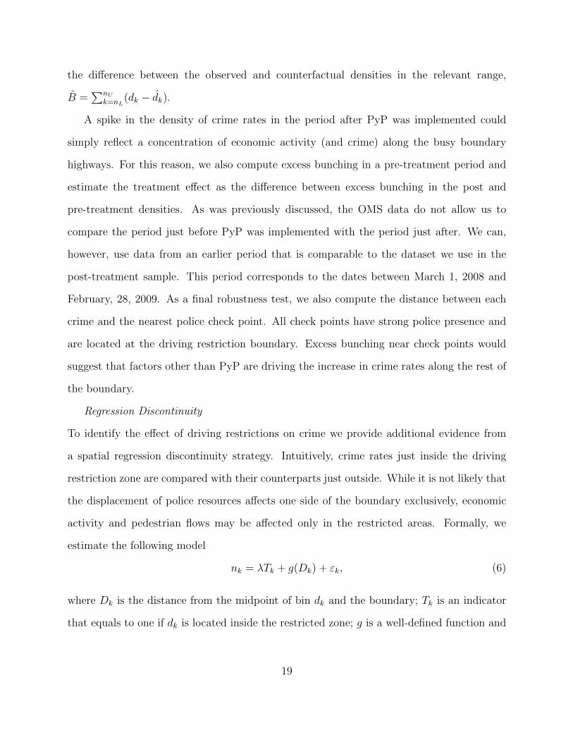
Regression Discontinuity

To identify the effect of driving restrictions on crime we provide additional evidence from

a spatial regression discontinuity strategy. Intuitively, crime rates just inside the driving

restriction zone are compared with their counterparts just outside. While it is not likely that

the displacement of police resources affects one side of the boundary exclusively, economic

activity and pedestrian flows may be affected only in the restricted areas. Formally, we

estimate the following model

nk = λTk + g(Dk) + εk, (6)

where Dk is the distance from the midpoint of bin dk and the boundary; Tk is an indicator

that equals to one if dk is located inside the restricted zone; g is a well-defined function and

19

ε captures all other unobservables that explain crime rates. We focus our attention on the

parameter λ, which captures the discontinuity at the driving restriction boundary.

For robustness and completeness, the function g is modeled in several ways. Besides

conventional linear, quadratic and cubic specifications, we also estimate models that allow

coefficients of these polynomials to vary on each side of the boundary. Moreover, models

are estimated using different “windows” that restrict the sample to crimes within 1000, 800,

600, 500 and 400 meters of the boundary. The choice of k is, to a certain extent, arbitrary.

For these reason, we estimate models for various values of k.

Again, to test the fundamental assumption that the discontinuity is related to PyP and

not to other unobserved factors, we also analyze crime rates near the boundary in a period

before PyP was implemented. These additional empirical tests should alleviate concerns

about omitted factors that might result in crime rates being systematically higher or lower

on one side of the boundary.

5 Results

5.1 Difference-in-Difference (DD)

In this section we estimate treatment effects using the DD strategy and our first source of

crime data (the National Police). Recall that these data can be compared before and after

treatment.

In all empirical models, the treatment group consists of working-day peak hours in Quito.

As we mentioned in Section 4.2.1, we consider three alternative control groups: a) non-

working-day peak hours in Quito, b) working-day off-peak hours in Quito, and c) working-

day peak hours in Guayaquil. Before presenting our results it is worth discussing the main

assumption underlying the DD strategy: the pre-treatment trends of treatment and control

groups should be parallel. To verify this assumption, we plot in each panel of Figure 4 the

20

evolution of the average number of crimes-per-hour for the treatment group and each of

the control groups, as well as the difference between this two. Despite the relatively short

pre-treatment period, it appears that the pre-treatment difference between treatment and

control groups is stationary.16

We estimate several versions of equation (2) and present results in Table 1. In all spec-

ifications, the dependent variable is the number of crimes h during peak hours in Quito–

between 7:00am and 9:59am, and between 4:00pm and 7:59pm. Our simplest specification in

column (1) includes a covariate that equals 1 if the crime measurement was taken after the

implementation of PyP (After); a variable that indicates a working day (Work); and the

treatment variable, PyP , that equals one during any working day peak hour in the treatment

period. This simple difference-in-difference pooled specification provides a useful benchmark

to interpret our coefficients. First note that peak-hour crime rates on workdays is notably

larger (about 1.04 crime per hour higher) than during weekends and holidays. Crimes are

also more likely to occur during the post-treatment period. The estimated coefficient of the

treatment variable, (α = 0.39), suggests that the average difference between the number

of weekday and weekend crimes per hour increased by 0.39 (about 9%) after imposition of

PyP. The standard errors, which are clustered at the week level to account for any potential

serial correlation between crime levels in consecutive hours, show that these estimates are

statistically significant almost at the 1% significance level. As shown in columns (2)-(5), the

estimate of α is notably robust when other covariates are added to the benchmark model.

For instance, the coefficient barely changes even when year-month fixed effects, day-of-the-

week fixed effects, hour-of-the-day fixed effects, day-hour interactions, and a comprehensive

set of weather covariates are included.

The results from estimating equation (3) are shown in Table 2. In this specification

16Given the short pre-treatment period, we do not report any formal tests to validate this assumption.(Once we cluster standar errors at the week level, we are unable to detect statistically significant differencesbetween the pre-treatment trends.)

21

we focus on the sample of working day hours in Quito. In the simplest specification in

column (1) we include a covariate that equals 1 during the post-treatment period (After),

a variable that indicates a peak hour (Peak), and the treatment variable, PyP . Notice

that the average number of crimes per-hour during the non-peak period increased by 1.02

after PyP introduction; crimes are also substantially more likely to occur during peak hours.

The estimated treatment effect (α = 0.23), suggests that the average difference between

the number of peak and non-peak crimes per hour increased by 0.23 (about 5%) after the

program implementation. As was the case with equation (2), the estimate of the treatment

effect does not change when other covariates are added to the basic model.

Finally, we estimate equation (4), which identifies treatment effects using crime rates

during working-day peak hours in Guayaquil as the counterfactual trend. The dependent

variable in all specifications is the total number of crimes during peak hours in Quito and

Guayaquil. Results shown in Table 3 highlight positive and large effects. For instance,

the difference in crime rates between Quito and Guayaquil during peak hours increased by

as much as 0.4 crimes per hour after PyP was introduced. This estimate is robust across

specifications and statistically significant at conventional levels.17

Crime data are only available from January 2010. Hence, the pre-treatment period (a

little over 4 months) is much shorter than the post-treatment (25 months). Most empirical

studies that analyze the effects of driving restrictions that exploit the policy discontinuity

have used a symmetric window of observations. As a robustness check, we take a similar

approach and estimate equations (2), (3) and (4) restricting the sample to observations

between January 1, 2010, and August 31, 2010. This gives us a symmetric window of 4

months before and after policy implementation. Results are shown in Table 4. Each row-

column combination in this table displays the coefficient of interest, i.e., the treatment effect

17We have not been able to collect hourly weather data in Guayaquil. For this reason, models do notinclude weather controls.

22

of a different model-specification, respectively. The estimated treatment effects using the

restricted sample range between 0.2 and 0.8 and, overall, are consistent with our previous

findings. Of course, given that the resticted sample includes only about 8 months of data,

the estimated effects could be reflecting seasonal trends in crime rates. Hence, the restricted

sample results should be interpreted with caution.

To assess whether the increase in crime rates during working-day peak hours is caused

by factors other than PyP, we estimate equations (2), (3) and (4) using several “placebo”

samples. The parameter α in equation (2) measures the change in the difference between

peak hour crime rates for working and non-working days in Quito. This parameter is now

estimated using the corresponding “placebo” sample of hours in Guayaquil. Results shown in

the first row of Table 5 show no statistically significant effect in any of the specifications. The

treatment effect estimated with equation (3) exploits differences between weekday peak and

off-peak crime rates in Quito. Again, we estimate the same model using data for Guayaquil

and show results of several specifications in the second row of Table 5. Results suggest that

the placebo treatment effect is close to zero in all specifications (−0.034) and statistically

insignificant. Finally, we estimate equation (4) using the sample of non-working days in both

Quito and Guayaquil. Because PyP affected working days only, one should not expect to

find any treatment effect in this placebo sample. As expected, results shown in the third

row of Table 5 confirm our priors.

In sum, the combined empirical evidence supports our hypothesis: Driving restrictions

can affect crime rates.

5.2 Spatial Distribution of Crime

In this section we exploit OMS property crime data and the identification strategy described

in Section 4.2.1 to identify the causal effect of PyP on crime. Recall that OMS data include

the geographic coordinates where a property crime occurred, allowing us to compute crime

23

rates on each side of the boundary.

Given Quito’s geography, we focus our attention on crimes that occurred within a 1 km

“window” of the driving restriction boundary. As shown in Figure 1, areas far to the East

and far to the West of the driving restriction are unpopulated. Moreover, in some areas, the

distance between the East and West boundaries is less than 4 km. Hence a “top window” of

1 km seems appropriate (as a starting point) to measure differences in crime rates on each

side of the driving restriction zone.

Figure 5 illustrates this approach: we would like to compute crime rates to the left and

to the right of the driving restriction boundary. The right panel displays the location of

crimes in the post-treatment calendar year. The left panel displays the location of crimes in

a pre-treatment period.18 From these figures alone, it is not possible to visualize any excess

bunching or discontinuity in crime rates across space, and it is hard to spot any differences

between the pre and post-treatment periods. The figures are useful, however, to identify the

areas in the city that are more prone to crime. Note that the driving restriction boundary

crosses unpopulated areas with very low or no crime occurrences, particularly in the east.

Hence, most of the crimes in our sample are located near the western boundary of the city.

5.2.1 Results: Bunching

In Figure 6 we compute the density of crime rates near the boundary. Each point in this

figure shows the average number of crimes per meter at that location, and the solid line

displays the counterfactual density estimated using the methods described in section 4.2.2.

The top panel computes the density for the pre-treatment period. It shows that the average

number of crimes per meter declines with distance-from-the-city-center. This is expected,

since population density is generally lower the further an area is from the central business

18Due to the way in which the OMS data were collected, we cannot compare the post-treatment periodwith the calendar year just before PyP was implemented. The closest calendar year to PyP implementationthat is comparable to the post-treatment data is the period between March 1, 2008 and February 28, 2009.

24

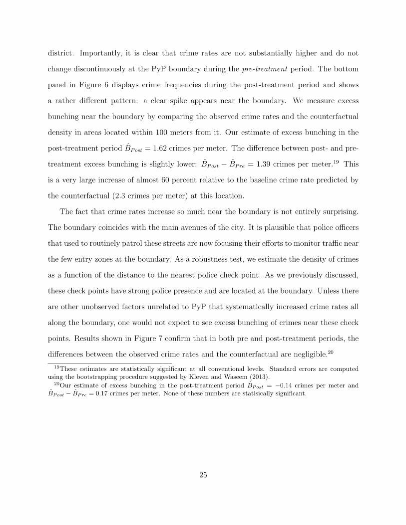
district. Importantly, it is clear that crime rates are not substantially higher and do not

change discontinuously at the PyP boundary during the pre-treatment period. The bottom

panel in Figure 6 displays crime frequencies during the post-treatment period and shows

a rather different pattern: a clear spike appears near the boundary. We measure excess

bunching near the boundary by comparing the observed crime rates and the counterfactual

density in areas located within 100 meters from it. Our estimate of excess bunching in the

post-treatment period BPost = 1.62 crimes per meter. The difference between post- and pre-

treatment excess bunching is slightly lower: BPost − BPre = 1.39 crimes per meter.19 This

is a very large increase of almost 60 percent relative to the baseline crime rate predicted by

the counterfactual (2.3 crimes per meter) at this location.

The fact that crime rates increase so much near the boundary is not entirely surprising.

The boundary coincides with the main avenues of the city. It is plausible that police officers

that used to routinely patrol these streets are now focusing their efforts to monitor traffic near

the few entry zones at the boundary. As a robustness test, we estimate the density of crimes

as a function of the distance to the nearest police check point. As we previously discussed,

these check points have strong police presence and are located at the boundary. Unless there

are other unobserved factors unrelated to PyP that systematically increased crime rates all

along the boundary, one would not expect to see excess bunching of crimes near these check

points. Results shown in Figure 7 confirm that in both pre and post-treatment periods, the

differences between the observed crime rates and the counterfactual are negligible.20

19These estimates are statistically significant at all conventional levels. Standard errors are computedusing the bootstrapping procedure suggested by Kleven and Waseem (2013).

20Our estimate of excess bunching in the post-treatment period BPost = −0.14 crimes per meter andBPost − BPre = 0.17 crimes per meter. None of these numbers are statisically significant.

25

5.2.2 Results: Regression Discontinuity

In Figure 8 we compute again the average crime frequency as a function of the distance to the

boundary, but also include a flexible non-parametric estimate of the density at each side of

the boundary. The bottom panel of this figure shows a large discontinuous “jump” just inside

the boundary. To compute the size of the jump, we estimate several versions of equation (6)

and present results in Table 6. The top and bottom panels display results for the pre-

and post-treatment periods, respectively. In both panels, each row and column combination

presents the estimate of λ, the treatment effect. Each column displays results from a different

“window” of observations, while each row corresponds to a different specification for the

function g. In all models, we set the number of bins, k, equal to the total window width.

Hence, the dependent variable is always the number of crimes in each one-meter-bin within

our “window.”

Results confirm the patterns observed in Figure 8. Before PyP, there is little evidence of

a discontinuous jump at the boundary. In the post-treatment period, however, crime rates

notably increase just inside the restriction zone. Both Bayesian Information Criteria (BIC)

and Akaike Information Criteria (AIC) have been computed and favor model (6) over the

others. Based on the estimates of model (6), PyP has increased the total number of crimes

just inside the boundary by as much as 5.5 per meter, over a 100% increase compared to

prevalent crime rates at the other side.

5.3 Discussion

The combined empirical evidence suggests that the introduction of PyP led to an increase

in crime rates in Quito. However, the magnitude of the effect depends on the identification

strategy we use. When spatial variation is exploited, results suggest that PyP led to a large

increase of crime rates near the boundary (60 to 100 percent). Caution must be exercised

26

when interpreting these results. While our findings show that crime along the boundary

drastically increased, we cannot assess if PyP raised the overall level of crime in the city. It

might well be that criminal activity was displaced from one part of the city to another. The

spatial models identify local effects at the boundary but cannot identify aggregate effects.

The difference-in-difference models, on the other hand, might assess the effect of PyP

on aggregate crime levels. And results point to much smaller (yet still large) treatment

effects. DD results suggest that the implementation of PyP increased crime levels (during

peak working day hours) by as much as 10%. Of course, results depend on the chosen

control group (counterfactual trend), and every potential control group can be subject to

criticism. For example, our second control group in the DD specification assumes that

crime trends during non-peak hours are a valid counterfactual trend in the absence of the

program. Because crimes could be displaced from off-peak to peak hours, however, this

fundamental assumption may fail. To alleviate such concerns, we compute results using

three alternative counterfactual trends. It is reassuring that results from all specifications

are generally consistent and point to a clear conclusion: the introduction of PyP increased

crime rates during peak hours in Quito.

5.4 Channels

As discussed in Section 2, driving restrictions have the potential to increase crime rates

during restricted times through two channels: Crime rates go up due to higher pedestrian

flows (ν1 increases) and/or due to a shift in police enforcement allocation resulting in lower

crime detection rates (θ1 decreases). How much have pedestrian flows and crime enforcement

changed after PyP? The answer to this question will help us understand the channels through

which driving restrictions influence criminal activity.

As noted in Section 3, there has been a substantial commitment of police resources to PyP

enforcement. Besides gathering in 12 strategic locations along the boundary, 15 additional

27

teams locate at random points inside the city. Moreover, driving restrictions enforcement

has been vigorous. As previously discussed, there have been tens of thousands of reported

violations during the first year of the program; the number of detected violations might be

much larger.21 It seems clear that enforcement of PyP imposed a non-negligible burden on

policing resources. At least in the short run, we would expect that policing resources were

shifted from other crime detection activities, decreasing θ1.

Ideally, to analyze the relationship between PyP and ν1 we would like to assess the

evolution of pedestrian flows in Quito since 2008. Unfortunately, these data are unavailable.

As an alternative, we evaluate the trend in the use of Quito’s main public transportation

system, the Trolebus. The Trolebus is a trolleybus system that has over 15 miles of dedicated

street lanes and is limited to North-South travel within the city. It serves more than 300

thousand passengers per day. Figure 9 plots the evolution of public transportation customers

since 2008. No obvious shift in the level or slope appears after May 2010, when PyP was

introduced.

PyP may induce drivers to use alternative forms of transportation, such as walking or

public transportation, during the days when they are subject to the driving restriction, and

make them more vulnerable to criminal activities. To test this hypothesis, we exploit the

administrative records of the Ecuadorian Police and Tax Authority to obtain the license

plate number of the vehicles owned by crime victims in Quito. Less than 10 percent of

crime victims own a car (registered under their name in the police records). We focus on

about 5,000 reported crimes whose victims owned fewer than three cars. Using a simple

multinomial logit we test if an individual is more likely to be a victim of crime on a day

when the use of one of the individulal’s vehicles is restricted. Formally, let Di ∈ {1, 2, 3...7}

be the day of the week when individual i was victimized, and let Xij be an indicator that

21Anecdotic evidence suggest that paying bribes to police officers to avoid fines for traffic violations is acommon practice in Ecuador, but one can only speculate about the size of this black market.

28

takes the value of one if individual i faced a driving restriction on day j. The multinomial

assumption implies that

Pr{Di = k} =eτj+γjXij

1 +7∑

k=2

eτk+γkXik

. (7)

The model is estimated using maximum likelihood. Interestingly, we cannot reject the

joint null hypothesis that all γj’s are equal to zero (p-value is 0.65); hence, there is no

evidence that individuals are more likely to be victimized on a day when they face driving

restrictions.

Summarizing, it is likely that policing resources devoted to crime detection and crime

prevention decreased after the introduction of PyP. On the other hand, we find no direct

evidence that the increase in crime rates is associated with higher pedestrian flows.

6 Conclusions

Driving restrictions have been a popular instrument in many cities around the world to al-

leviate pollution and congestion problems. While there is mixed evidence in the literature

about the effectiveness of these programs to improve air quality and alleviate congestion,

our study is the first to document an important side-effect: increasing crime. Programs that

restrict vehicle flows may primarily affect criminal activity because program enforcement

is costly and can potentially displace resources used for crime prevention and crime detec-

tion. Driving restrictions may also raise pedestrian flows, increasing the number of potential

victims.

To test these hypotheses we evaluate the effect of Quito’s Pico y Placa program on

crime. Our identification strategy exploits both temporal and spatial variation in the imple-

mentation of the program. Findings provide credible evidence that driving restrictions can

29

increase crime. For instance, results from a DD identification strategy suggests that crime

rates during the time period when PyP is in effect increased between 5% and 10% after the

introduction of PyP. We see no changes when the DD models are estimated with “placebo”

samples. Furthermore, the post-treatment density of crime shows substantial excess mass

near the boundary of the driving restriction zone, particularly in the area just inside the

boundary. These patterns are not present during the pre-treatment period. In our view, the

combined empirical evidence presented in this paper supports our main hypothesis: Driving

restrictions can affect crime rates.

The use of driving restrictions has been an attractive non-market policy to deal with

congestion problems. Our study warns about non-negligible side-effects produced by these

programs given high (opportunity) costs of enforcement. Given a fixed stock of resources to

jointly monitor traffic regulations and criminal activity, policy makers in cities with driving

restrictions may have to choose between congestion or crime, until other (perhaps market

oriented) mechanisms are implemented to solve these urban problems.

30

References

ADMQ (2010). Resolucion A 0017, Alcaldia Distrito Metropolitano de Quito (ADMQ).

Becker, G. S. (1968). Crime and punishment: An economic approach. Journal of PoliticalEconomy, 76(2):169–217.

Benson, B. L., Kim, I., Rasmussen, D. W., and Zhehlke, T. W. (1992). Is property crimecaused by drug use or by drug enforcement policy? Applied Economics, 24(7):679–692.

Benson, B. L. and Rasmussen, D. W. (1991). Relationship between illicit drug enforcementpolicy and property crimes. Contemporary Economic Policy, 9(4):106–115.

Benson, B. L., Rasmussen, D. W., and Kim, I. (1998). Deterrence and Public Policy: Trade-Offs in the Allocation of Police Resources. International Review of Law and Economics,18(1):77–100.

Bonilla, J. A. (2011). Effects of the Increased Stringency of Driving Restrictions on AirQuality and Car Use in Bogota. Working paper, Department of Economics, University ofGothenburg.

Carrillo, P. E., Malik, A. S., and Yoo, J. (2015). Driving Restrictions That Work? Quito’sPico y Placa Program. Canadian Journal of Economics, forthcoming.

Carrillo, P. E., Pomeranz, D., and Singhal, M. (2014). Dodging the taxman: Firm misre-porting and limits to tax enforcement. NBER Working Papers 20624, National Bureau ofEconomic Research.

Chen, Y., Jin, G. Z., Kumar, N., and Shi, G. (2011). The promise of Beijing: Evaluating theimpact of the 2008 olympic games on air quality. Working Paper 16907, National Bureauof Economic Research.

Davis, L. W. (2008). The Effect of Driving Restrictions on Air Quality in Mexico City.Journal of Political Economy, 116(1):38–81.

de Grange, L. and Troncoso, R. (2011). Impacts of vehicle restrictions on urban transportflows: The case of Santiago, Chile. Transport Policy, 18(6):862 – 869.

DiTella, R. and Schargrodsky, E. (2004). Do Police Reduce Crime? Estimates Using the Al-location of Police Forces After a Terrorist Attack. American Economic Review, 94(1):115–133.

Draca, M., Machin, S., and Witt, R. (2011). Panic on the streets of london: Police, crime,and the july 2005 terror attacks. American Economic Review, 101(5):2157–2181.

EMMOP (2011). Pico y placa se mantiene sin cambios en la programacion. Boletın deprensa, june 29, 2011, Empresa Municipal de Movilidad y Obras Publicas (EMMOP).

31

EMMOP (2012). Se actualizan valores de multas para pico y placa. Boletın de prensa,january 3, 2012, Empresa Municipal de Movilidad y Obras Publicas (EMMOP).

Eskeland, G. S. and Feyzioglu, T. (1997). Rationing can backfire: The “day without a car”in Mexico City. The World Bank Economic Review, 11(3):383–408.

Gallego, F., Montero, J.-P., and Salas, C. (2013). The effect of transport policies on car use:Evidence from latin american cities. Journal of Public Economics, 107:47 – 62.

Kleven, H. J. and Waseem, M. (2013). Using Notches to Uncover Optimization Frictionsand Structural Elasticities: Theory and Evidence from Pakistan. The Quarterly Journalof Economics, 128(2):669–723.

Lin, C.-Y. C., Zhang, W., and Umanskaya, V. I. (2011). The Effects of Driving Restrictionson Air Quality: Sao Paulo, Bogota, Beijing, and Tianjin. 2011 Annual Meeting, July 24-26,2011, Pittsburgh, Pennsylvania 103381, Agricultural and Applied Economics Association.

OMS (2010). Informe segundo semestre del 2010. Informe 15, Observatorio Metropolitantode Seguridad Ciudadana (OMS).

Troncoso, R., de Grange, L., and Cifuentes, L. A. (2012). Effects of environmental alerts andpre-emergencies on pollutant concentrations in Santiago, Chile. Atmospheric Environment,61(0):550 – 557.

Viard, V. B. and Fu, S. (2015). The effect of Beijing’s driving restrictions on pollution andeconomic activity. Journal of Public Economics, 125:98 – 115.

Yang, D. (2008). Can enforcement backfire? crime displacement in the context of customsreform in the Philippines. Review of Economics and Statistics, 90(1):1 – 14.

32

Figure 1:Driving Restriction Boundary

!!

!

!

!

!

!

!!

!

ÜLegend! Checkpoints

Limit PyPStreetsQuito Populated Area

0 3.5 7 10.51.75Kilometers

Notes: This Figure shows the Pico y Placa driving restriction boundary in Quito, Ecuador. Dashed linesdenote the boundary in areas with no population.

33

Figure 2:Police Crime Data: Quito vs. Guayaquil

6

4

5

er h

our

3

4

of c

rim

es p

e

2

3

age

num

ber

1

Aver

a

0

18 14 10 -6 -2 2 6 10 14 18 22 26 30 34 38 42 46 50 54 58 62 66 70 74 78 82 86 90 94 98 02 06- - - 1 1Number of Weeks After the Introduction of Pico y Placa

Guayaquil Quito

34

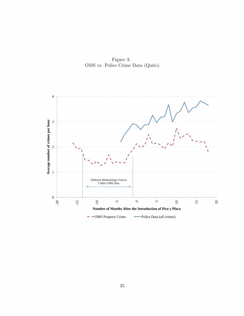
Figure 3:OMS vs. Police Crime Data (Quito)

4

3

r ho

ur

2of c

rim

es p

er

2

age

num

ber

o

1Aver

a

Different Methodology Used to Collect OMS Data

0

20 15 10 -5 0 5 10 15 20-2 -1 -1 - 1 1 2

Number of Months After the Introduction of Pico y Placa

OMS Property Crime Police Data (all crimes)

35

Figure 4:Average Number of Crimes Per Hour

−2

02

46

8N

umbe

r of

crim

es p

er h

our

−50 0 50 100Number of weeks since introduction of PyP

Working day Non−Working Day Difference

A. Quito: Peak Hours

−2

02

46

8N

umbe

r of

crim

es p

er h

our

−50 0 50 100Number of weeks since introduction of PyP

Peak Off−Peak Difference

B. Quito: Working Days

−2

02

46

8N

umbe

r of

crim

es p

er h

our

−50 0 50 100Number of weeks since introduction of PyP

Quito Guayaquil Difference

C. Working Days: Peak Hours

Notes: Figure shows the average number of crimes per hour for different samples in Quito and Guayaquil.Crime rate during (working day) peak hours in Quito, the treatment group, is compared with crime ratesfor three potential counterfactual control groups: a) non-working day peak hours in Quito, b) working dayoff-peak hours in Quito, and b) working day peak hours in Guayaquil.

36

Figure 5:Location of Property Crimes Near PyP Boundary

Before PyPPeriod: 3/1/2008 − 2/28/2009

After PyPPeriod: 5/3/2010 − 5/2/2011

Notes: Each point shows the location of a property crime within 1 km of the driving restriction boundary (solid line). Sample includes allproperty crimes (excluding vehicle thefts)reported to the police. The pre-treatment period is between 3/1/2008 and 2/28/2009. The year afterPyP corresponds to the period between 5/3/2010 and 5/2/2011.

37

Figure 6:Average Crime Frequency as a Function of Distance To Boundary: Property Crimes

Excess Bunching at the Boundary

02

46

810

Num

ber

of c

rimes

per

met

er

−1000 −500 0 500 1000Distance to Driving Restriction Boundary (Meters)

Non−parametric Counterfactual

Before PyPPeriod: 3/1/2008 − 2/28/2009

02

46

810

Num

ber

of c

rimes

per

met

er

−1000 −500 0 500 1000Distance to Driving Restriction Boundary (Meters)

Non−parametric Counterfactual

After PyPPeriod: 5/3/2010 − 5/2/2011

− Each bin has a 25 m length −

Notes: Each point shows the number of crimes per meter within the bin. Negative (positive) values denote areas inside (outside) the restrictedzone. The vertical line shows the driving restriction boundary. Sample includes all property crimes (excluding vehicle thefts) reported to thepolice. Solid line is a parametric estimate of the crime density excluding crimes within 100 meters of the boundary (see text for details). Thepre-treatment period is between 3/1/2008 and 2/28/2009. The year after PyP corresponds to the period between 5/3/2010 and 5/2/2011.

38

Figure 7:Average Crime Frequency as a Function of Distance To Nearest Police Check Point: Property Crimes

Excess Bunching at the Boundary

01

23

4N

umbe

r of

crim

es p

er m

eter

−1000 −500 0 500 1000Distance to Nearest Check Point (Meters)

Non−parametric Counterfactual

Before PyPPeriod: 3/1/2008 − 2/28/2009

01

23

4N

umbe

r of

crim

es p

er m

eter

−1000 −500 0 500 1000Distance to Nearest Check Point (Meters)

Non−parametric Counterfactual

After PyPPeriod: 5/3/2010 − 5/2/2011

− Each bin has a 25 m length −

Notes: Each point shows the number of crimes per meter within the bin. Each bin denotes the distance to the nearest PyP police check point(which are located at the boundary). Negative (positive) values denote areas inside (outside) the restricted zone. The vertical line shows thedriving restriction boundary. Sample includes all property crimes (excluding vehicle thefts) reported to the police. Solid line is a parametricestimate of the crime density excluding crimes within 100 meters of the boundary (see text for details). The pre-treatment period is between3/1/2008 and 2/28/2009. The year after PyP corresponds to the period between 5/3/2010 and 5/2/2011.

39

Figure 8:Average Crime Frequency as a Function of Distance To Boundary: Property Crimes

Discontinuous Jump at the Boundary After PyP

02

46

810

Num

ber

of c

rimes

per

met

er

−1000 −500 0 500 1000Distance to Driving Restriction Boundary (Meters)

Before PyPPeriod: 3/1/2008 − 2/28/2009

02

46

810

Num

ber

of c

rimes

per

met

er

−1000 −500 0 500 1000Distance to Driving Restriction Boundary (Meters)

After PyPPeriod: 5/3/2010 − 5/2/2011

− Each bin has a 25 m length −

Notes: Each point shows the number of crimes within the bin. Negative (positive) values denote areas inside (outside) the restricted zone.The vertical line shows the driving restriction boundary. Sample includes all property crimes (excluding vehicle thefts) reported to the police.Solid lines are non parametric estimates of relationship. The pre-treatment period is between 3/1/2008 and 2/28/2009. The year after PyPcorresponds to the period between 5/3/2010 and 5/2/2011.

40

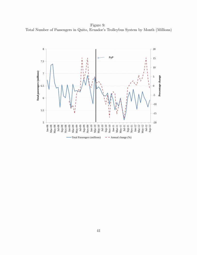
Figure 9:Total Number of Passengers in Quito, Ecuador’s Trolleybus System by Month (Millions)

15

208

PyP

10

7

7.5

ns)

0

5

6.5

7

age

chan

ge

gers

(mill

ion

-5

0

6

6.5

Perc

enta

Tota

l pas

seng

-15

-10

5.5

T

-20

-15

5

08 08 08 08 08 08 09 09 09 09 09 09 10 10 10 10 10 10 11 11 11 11 11 11 12 12 12 12 12

Jan-

0M

ar-0

May

-0Ju

l-0Se

p-0

Nov

-0Ja

n-0

Mar

-0M

ay-0

Jul-0

Sep-

0N

ov-0

Jan-

1M

ar-1

May

-1Ju

l-1Se

p-1

Nov

-1Ja

n-M

ar-

May

-Ju

l-Se

p-N

ov-

Jan-

1M

ar-1

May

-1Ju

l-1Se

p-1

Total Passengers (millions) Annual change (%)

41

PyP: Workday * After 0.385 ** 0.381 ** 0.387 ** 0.387 ** 0.405 **

(0.154) (0.164) (0.159) (0.160) (0.163)

After: 1 (Current Date > Policy Implementation) 0.868 ***

(0.178)

Workday: 1 (Working Day) 1.044 *** 1.055 *** 1.543 *** 1.543 *** 1.591 ***

(0.128) (0.139) (0.221) (0.222) (0.227)

Month-Year Interactions (29) NO YES YES YES YESDay-of-the-week fixed effects (6) NO NO YES YES YESHour-of-the-day fixed effects (23) NO NO YES YES YESDay-Hour Interactions NO NO NO YES YESWeather variables NO NO NO NO YES

Number of Observations 6,174 6,174 6,174 6,174 6,141R2 0.079 0.134 0.283 0.304 0.307

This table analyzes the relationship between hourly crimes and driving restrictions. The dependentvariable is the number of crimes reported to the police for each peak hour in Quito between January 1,2010 and May 31, 2012. A new driving policy was implemented on 5/3/2010. This policy imposeddriving restrictions during non-holiday weekday peak hours (working days). In our study, peak hours arethose between 7am and 9:59am and between 4pm and 7:59pm. Weather variables include temperature,rain, wind speed, solar radiation, relative humidity, their square, cubic and quartic terms. Sample isrestricted to peak hours. Sample size is smaller in last column due to missing observations (weathervariables). Standard errors (in parenthesis) have been clustered at the week level. *, **, ***, denotesignificance at the 10, 5, and 1 percent level, respectively.

Table 1: Effect of Driving Restrictions (PyP) on Crime Using Non-Working Days as Control

(1) (2) (3) (4) (5)

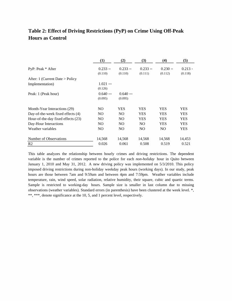
PyP: Peak * After 0.233 ** 0.233 ** 0.233 ** 0.230 ** 0.213 *

(0.110) (0.110) (0.111) (0.112) (0.118) After: 1 (Current Date > Policy Implementation) 1.021 ***

(0.126) Peak: 1 (Peak hour) 0.640 *** 0.640 ***

(0.095) (0.095)

Month-Year Interactions (29) NO YES YES YES YESDay-of-the-week fixed effects (4) NO NO YES YES YESHour-of-the-day fixed effects (23) NO NO YES YES YESDay-Hour Interactions NO NO NO YES YESWeather variables NO NO NO NO YES

Number of Observations 14,568 14,568 14,568 14,568 14,453R2 0.026 0.061 0.508 0.519 0.521

This table analyzes the relationship between hourly crimes and driving restrictions. The dependentvariable is the number of crimes reported to the police for each non-holiday hour in Quito betweenJanuary 1, 2010 and May 31, 2012. A new driving policy was implemented on 5/3/2010. This policyimposed driving restrictions during non-holiday weekday peak hours (working days). In our study, peakhours are those between 7am and 9:59am and between 4pm and 7:59pm. Weather variables includetemperature, rain, wind speed, solar radiation, relative humidity, their square, cubic and quartic terms.Sample is restricted to working-day hours. Sample size is smaller in last column due to missingobservations (weather variables). Standard errors (in parenthesis) have been clustered at the week level. *,**, ***, denote significance at the 10, 5, and 1 percent level, respectively.

Table 2: Effect of Driving Restrictions (PyP) on Crime Using Off-Peak Hours as Control

(1) (2) (3) (4) (5)

PyP: Quito * After 0.402 * 0.402 ** 0.402 ** 0.402 **

(0.227) (0.181) (0.181) (0.181) After: 1 (Current Date > Policy Implementation) 0.852 ***

(0.144) Quito: 1 (Quito) 0.524 *** 0.524 *** 0.524 *** 0.524 ***

(0.200) (0.161) (0.162) (0.162)

Month-Year Interactions (29) NO YES YES YESDay-of-the-week fixed effects (4) NO NO YES YESHour-of-the-day fixed effects (23) NO NO YES YESDay-Hour Interactions NO NO NO YES

Number of Observations 8,498 8,498 8,498 8,498R2 0.049 0.088 0.211 0.221

This table analyzes the relationship between hourly crimes and driving restrictions. Thedependent variable is the number of crimes reported to the police for each peak hour in Quitoand Guayaquil between January 1, 2010 and May 31, 2012. A new driving policy wasimplemented on 5/3/2010. This policy imposed driving restrictions during non-holidayweekday peak hours (working days) in Quito. In our study, peak hours are those between 7amand 9:59am and between 4pm and 7:59pm. Sample is restricted to peak hours in both cities.Standard errors (in parenthesis) have been clustered at the city-week level. *, **, ***, denotesignificance at the 10, 5, and 1 percent level, respectively.

Table 3: Effect of Driving Restrictions (PyP) on Crime Using Working Day Peak Hours in Guayaquil as Control

(1) (2) (3) (4)

Model

Model (1) : Using non-working day peak hours in Quito as control 0.205 0.205 0.235 0.235 0.203

(0.215) (0.224) (0.219) (0.222) (0.212) Model (2) : Using working day off-peak hours in Quito as control 0.406 ** 0.406 ** 0.406 ** 0.402 ** 0.400 **

(0.176) (0.176) (0.177) (0.180) (0.187) Model (3) : Using peak hours in Guayaquil as control 0.810 *** 0.810 *** 0.810 *** 0.810 ***

(0.283) (0.246) (0.246) (0.247)

Month-Year Interactions NO YES YES YES YESDay-of-the-week fixed effects (6) NO NO YES YES YESHour-of-the-day fixed effects (23) NO NO YES YES YESDay-Hour Interactions NO NO NO NO YESWeather variables NO NO NO NO YES

Each column-row combination in this table displays the coefficient of interest, i.e., the treatment effect of adifferent model specification. A new driving policy was implemented on 5/3/2010. The sample is restricted to4 months before and after PyP implementation. The dependent variable in all models is the number of crimesreported to the police by hour-of-the-day. Standard errors (in parenthesis) have been clustered at the week-citylevel. *, **, ***, denote significance at the 10, 5, and 1 percent level, respectively.

Table 4: Estimating Treatment Effects Using Symmetric Samples

(1) (2) (3) (4) (5)

Model / Sample

Model (1) using Guayaquil sample 0.178 0.162 0.177 0.177(0.235) (0.212) (0.209) (0.210)

Model (2) using Guayaquil sample -0.034 -0.034 -0.034 -0.034(0.099) (0.099) (0.099) (0.099)

Model (3) using Non-Working day sample 0.195 0.125 0.133 0.133

(0.300) (0.199) (0.192) (0.193)

Month-Year Interactions (29) NO YES YES YESDay-of-the-week fixed effects (6) NO NO YES YESHour-of-the-day fixed effects (23) NO NO YES YESDay-Hour Interactions NO NO NO YESWeather variables NO NO NO NO

Each column-row combination in this table displays the coefficient of interest, i.e., the treatmenteffect of a different model specification. A new driving policy in Quito was implemented on5/3/2010. The dependent variable in all models is the total number of crimes reported to thepolice by hour-of-the-day. Models reported in Tables (1), (2) and (3) are estimated using samplesnot directly affected by PyP. Standard errors (in parenthesis) have been clustered at the week-city level. *, **, ***, denote significance at the 10, 5, and 1 percent level, respectively.

Table 5: Effect of Driving Restrictions (PyP) on Crime Using "Placebo" Samples

(1) (2) (3) (4)

Table 6: Effect of PyP on Property Crime: RD EstimatesDependent variable is the number of crimes

A] Pre-Treatment Period

Model 1000 800 600 500 400

1) Linear 0.845 *** 1.042 *** 0.709 *** 0.413 * 0.049(0.156) (0.178) (0.209) (0.231) (0.260)

2) Quadratic 0.845 *** 1.042 *** 0.709 *** 0.413 * 0.049(0.156) (0.175) (0.205) (0.227) (0.257)

3) Cubic 0.930 *** 0.318 -0.252 -0.523 -0.929 **

(0.221) (0.243) (0.284) (0.320) (0.372)4) Linear x Treatment 0.845 *** 1.042 *** 0.709 *** 0.413 * 0.049

(0.155) (0.174) (0.204) (0.226) (0.256)5) Quadratic x Treatment 0.719 *** -0.036 -0.618 * -0.866 ** -1.200 ***

(0.245) (0.274) (0.325) (0.369) (0.428)6) Cubic x Treatment -0.924 *** -1.068 *** -1.259 *** -1.394 *** -1.138 *

(0.339) (0.392) (0.475) (0.532) (0.609)Model with lowest AIC 6 6 6 6 6Model with lowest BIC 6 6 5 3 3

Number of Observations 2,000 1,600 1,200 1,000 800

B] Post-Treatment Period

Model 1000 900 750 500 400

Linear 0.794 *** 1.457 *** 1.676 *** 1.927 *** 2.144 ***

(0.231) (0.272) (0.340) (0.391) (0.467)Quadratic 0.794 *** 1.457 *** 1.676 *** 1.927 *** 2.144 ***

(0.232) (0.263) (0.327) (0.374) (0.442)Cubic 1.877 *** 2.038 *** 2.531 *** 2.721 *** 3.336 ***

(0.360) (0.418) (0.519) (0.594) (0.695)Linear x Treatment 0.794 *** 1.457 *** 1.676 *** 1.927 *** 2.144 ***

(0.229) (0.256) (0.316) (0.359) (0.420)Quadratic x Treatment 2.309 *** 2.363 *** 2.943 *** 3.198 *** 3.906 ***

(0.380) (0.448) (0.537) (0.601) (0.676)Cubic x Treatment 3.168 *** 3.470 *** 4.123 *** 4.947 *** 5.513 ***

(0.555) (0.637) (0.737) (0.786) (0.869)Model with lowest AIC 6 6 6 6 6Model with lowest BIC 6 6 6 6 6

Number of Observations 2,000 1,600 1,200 1,000 800

Maximum Distance to Driving Restriction Boundary (m)

Maximum Distance to Driving Restriction Boundary (m)

Note: Each cell in this table displays the treatment effect using a particular model and sample combination. Panel A measures the discontinuity in the density of crime rates at the PyP boundary before the driving restriction was introduced. The second panel measures the discontinuity after the program started. Robust standard errors are shown in parenthesis. *, **, and *** denote significance at the 10, 5 and 1 percent level, respectively.