University of CalgaryPHYS 443: Quantum Mechanics I

Polarization state measurement and tomography

Laboratory experiment

1 Purpose

• To understand the concepts of optical wave polarization;

• to become familiar with optical polarization instruments, such as the half- and quarter-waveplates and the polarizing beam splitter;

• to experimentally test the Measurement Postulate of quantum mechanics;

• to practice the application of operators to calculate transformations of quantum states;

• to experimentally reconstruct an unknown quantum state through measurements.

2 Equipment

• optical bench;

• 2 photodetectors connected to multimeters;

• helium-neon Laser;

• polarizing beam splitter (PBS);

• 2 half-wave plates (HWP);

• 2 quarter-wave plates (QWP)

3 Safety advice

Never look directly into the laser beam.

4 Equipment care and maintenance

Every optical element in this experiment costs several hundred dollars. Exercising proper care isessential for maintaining the experiment in a proper operational condition for future generations ofstudents.

It is most important to avoid touching optical surfaces. If you do happen to accidentally touch asurface and leave a fingerprint, inform the lab manager immediately to have it cleaned. If you don’tnotice / forget / neglect to clean it, your body fat residue will enter a chemical reaction with theglass surface and damage it permanently after a few hours.

Another important advice is not to lay your optical elements flat on the table. Even a briefexposure to dust can permanently damage them. Whenever you remove an optic from the apparatus,place it in a holder or lay it down sideways, so the surfaces are vertical.

Do not forget to replace protective covers on your optics when you are leaving the lab.

1

5 Introductory note

This experiment deals with macroscopic quantities of light. All the results you are about to see canbe explained by means of classical electromagnetic wave theory. However, because our goal is tounderstand quantum mechanics, this manual is written in terms of quantum polarization states ofsingle photons. Because each photon in an electromagnetic wave has the same polarization state,macroscopic measurements on large numbers of photons, such as those performed here, reflect thequantum behavior of each individual photon.

The theory behind optical polarization states, quantum measurements and tomography is ex-plained in Chapter 1 and Appendix C of the lecture notes.

6 Procedure

6.1 Preparation and alignment

a) Remove protective covers from the optics. Remember to replace them when finished.

b) Make sure the photodetectors are connected to power supplies and multimeters. Set thephotodetectors’ resistance to 3.3 kΩ. Make sure the power supplies and multimeters are turnedon. Set the multimeters’ limits to 2 Volts.

c) Turn on the laser. Align the laser beam parallel to the optical bench.

d) Place one of the photodetectors onto the optical bench about 30 cm in front of the laser. Alignthe detector so that the laser shines into the center of the detector’s sensitive area.

The multimeter’s reading should be on the order of −1 Volt with the laser beam present and0 when it is blocked (the negative sign is hereafter omitted). Move the photodetector in thetransverse plane by ±1 mm and check that the voltage reading does not change by more thana few per cent.

e) Place the PBS ∼ 5 cm immediately before the detector. Because the laser is vertically polar-ized, the PBS should reflect the beam almost completely. Check that the voltmeter readingfor the transmitted beam is less than 5% of the value measured without the PBS.

f) Place the second detector into the reflected beam. Make sure the beam hits the detector’ssensitive area by repositioning the detector and/or tweaking the PBS mount screws. Check thereading on the corresponding multimeter to be on the order of 1 Volt. Move the photodetectorin the transverse plane by ±1 mm and check that the voltage reading does not change by morethan a few per cent.

Try to avoid bumping the laser, PBS and detectors for the remainder of the experiment. Other-wise you may have to repeat the above alignment procedure.

6.2 Measuring linear polarization in the canonical basis

You have set up an apparatus for measuring the polarization in the canonical basis. Our next goalis to use this apparatus to measure various linearly polarized states.

detectors

horizontalpolarization

verticalpolarization

laser

HWP1 PBS

preparation measurement

2

a) Place one of the half-waveplates (HWP1) in front ot the PBS. For consistency, orient allwaveplates so that the rotor of the waveplate frame is facing the laser.

b) Rotate the HWP to minimize the transmission of the laser through the PBS. This means thatthe HWP is not changing the laser’s polarization state, so the vertical laser polarization iseither purely ordinary or purely extraordinary with respect to that waveplate. This means thewaveplate’s optic axis is either horizontal or vertical.

For the physics we are studying here, it does not matter whether the orientation of the optic axisis horizontal or vertical. Indeed, if the matrix of the half-waveplate operator with a horizontal

optic axis in the canonical basis is AHWP(0) '(−1 00 1

), then the same waveplate with

the optic axis oriented vertically it is AHWP(90) '(

1 00 −1

). The photon states obtained

through the action of these two operators are different only by the unphysical overall phasefactor −1. As a matter of convention, we shall assume the optic axis in the present positionof the waveplate to be horizontal.

Record the angle reading βHWP1 on the waveplate frame. Although the optic axis is horizontal,this reading may not equal zero because the waveplate is glued to the frame at a randomangle. For any other reading β, the angle between the waveplate’s axis and the horizontal isα = β − βHWP1

.

Tips:

• Write down the number on the sticker attached to the waveplate.

• Do not use any markings on the wavelpate frame to determite the optic axis angle. Thesemarkings are not reliable.

c) Record the voltage Vr,max of the multimeter in the reflected channel.

Then rotate the waveplate by about 45 to turn the polarization to horizontal. Make a fineadjustment to the waveplate to minimize the reflection from the PBS. Record the voltageVt,max of the multimeter in the transmitted channel.

We shall refer to the procedure of measuring Vt,max and Vr,max as calibrating the detectors.Keep in mind that the calibration values may drift during the measurement run. You maywish to re-calibrate your detectors both before and after each series of data, and perhapseven a few times during the data run. Also, the detectors should be re-calibrated for everydata acquisition run with a different set of waveplates because the waveplates are partiallyabsorptive.

d) Rotate the waveplate to prepare a set of linearly polarized states |θ〉. The waveplate fill “flip”the vertically polarized input photon about its optic axis. If the optic axis is at the angleα = β − βHWP1

to horizontal, you will produce a photon linearly polarized at θ = 2α − 90

with respect to horizontal. For each θ, measure the voltage in the transmitted and reflectedchannels, Vt and Vr, respectively, as a function of the waveplate angle β. These voltagestranslate into photon detection probabilities according to prt = Vt/Vt,max and prr = Vr/Vr,max.

Record your data into Table 1. Plot the experimentally acquired prt and prr as a function ofθ together with theoretical curves:

prt = | 〈H| θ〉 |2 =

∣∣∣∣( 1 0)( cos θ

sin θ

)∣∣∣∣2 = cos2 θ;

prr = | 〈V | θ〉 |2 =

∣∣∣∣( 0 1)( cos θ

sin θ

)∣∣∣∣2 = sin2 θ.

3

The last column in the table is for self-check. If you get a value that is significantly differentfrom 1, you are doing something wrong; probably the detectors are not correctly calibrated.

A typical error observed in these experiments should not exceed a few per cent. If the behavioryou see is dramatically different from the theoretically expected, stop and think!

6.3 Measuring linear polarization in the diagonal basis

laser

HWP1 PBS

preparation measurement

HWP2

a) Remove HWP1. Place another half-waveplate (HWP2) in front ot the PBS. Record the angleβHWP2 for which no polarization rotation is taking place. Again, we shall assume that thisangle corresponds to the optic axis being horizontal.

b) Rotate the waveplate by angle 22.5. In this position, the waveplate will transform photonpolarization states according to |+45〉 → |H〉, |−45〉 → |V 〉, thereby facilitating measurementin the diagonal basis.

c) Reinsert HWP1 in front of HWP2. Similarly to the previous subsection, use HWP1 to preparedifferent linear polarization states |θ〉. Perform measurements of these states in the diagonalbasis. Acquire the data into Table 1. Plot the experimentally acquired prt and prr as afunction of θ together with theoretical curves: prt = | 〈+45| θ〉 |2 and prr = | 〈−45| θ〉 |2.This time, please derive the theoretical expression independently.

In order to calibrate the detectors, you can temporarily set HWP1 to angle βHWP1and HWP2 to

βHWP2or βHWP2

+45. In this way, the first waveplate will not affect the laser’s vertical polarizationand the second one will either keep it vertical or rotate to horizontal. You may wish to adjust thewaveplates a bit in order to minimize the amount of light going to the other detector.

6.4 Measuring linear polarization in the circular basis

laser

HWP1 PBS

preparation measurement

QWP1

a) Remove both HWPs. Place a quarter-waveplate (QWP1) in front ot the PBS. Record the angleβQWP1

for which no polarization transformation is taking place. Again, let us assume that thisangle corresponds to the horizontal orientation of the optic axis (in the case of quarter-waveplates, there is a subtlety that we shall address later, but for now, let us use this assumption).

b) Rotate the QWP by 45. In this position, the waveplate will transform photon polarizationstates according to |L〉 → |H〉, |R〉 → |V 〉, thereby facilitating measurement in the circular

4

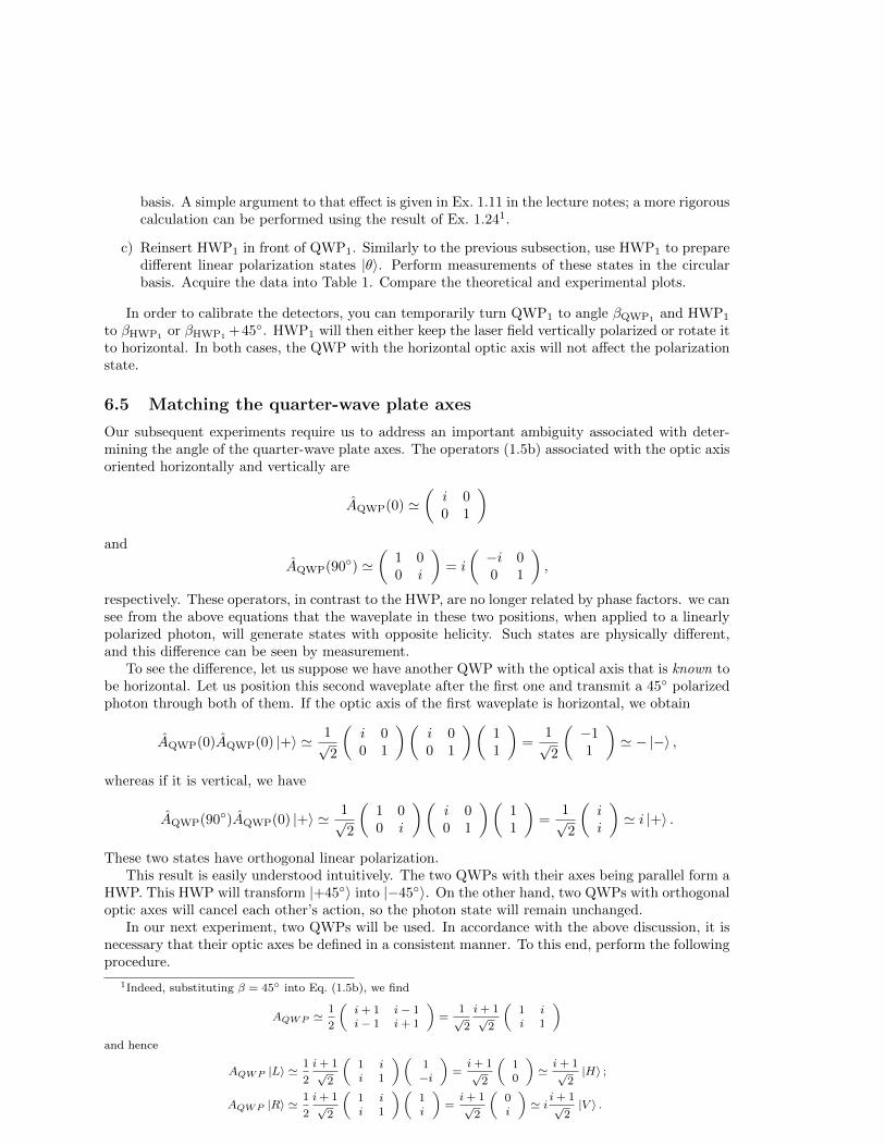
basis. A simple argument to that effect is given in Ex. 1.11 in the lecture notes; a more rigorouscalculation can be performed using the result of Ex. 1.241.

c) Reinsert HWP1 in front of QWP1. Similarly to the previous subsection, use HWP1 to preparedifferent linear polarization states |θ〉. Perform measurements of these states in the circularbasis. Acquire the data into Table 1. Compare the theoretical and experimental plots.

In order to calibrate the detectors, you can temporarily turn QWP1 to angle βQWP1and HWP1

to βHWP1 or βHWP1 +45. HWP1 will then either keep the laser field vertically polarized or rotate itto horizontal. In both cases, the QWP with the horizontal optic axis will not affect the polarizationstate.

6.5 Matching the quarter-wave plate axes

Our subsequent experiments require us to address an important ambiguity associated with deter-mining the angle of the quarter-wave plate axes. The operators (1.5b) associated with the optic axisoriented horizontally and vertically are

AQWP(0) '(

i 00 1

)and

AQWP(90) '(

1 00 i

)= i

(−i 00 1

),

respectively. These operators, in contrast to the HWP, are no longer related by phase factors. we cansee from the above equations that the waveplate in these two positions, when applied to a linearlypolarized photon, will generate states with opposite helicity. Such states are physically different,and this difference can be seen by measurement.

To see the difference, let us suppose we have another QWP with the optical axis that is known tobe horizontal. Let us position this second waveplate after the first one and transmit a 45 polarizedphoton through both of them. If the optic axis of the first waveplate is horizontal, we obtain

AQWP(0)AQWP(0) |+〉 ' 1√2

(i 00 1

)(i 00 1

)(11

)=

1√2

(−11

)' − |−〉 ,

whereas if it is vertical, we have

AQWP(90)AQWP(0) |+〉 ' 1√2

(1 00 i

)(i 00 1

)(11

)=

1√2

(ii

)' i |+〉 .

These two states have orthogonal linear polarization.This result is easily understood intuitively. The two QWPs with their axes being parallel form a

HWP. This HWP will transform |+45〉 into |−45〉. On the other hand, two QWPs with orthogonaloptic axes will cancel each other’s action, so the photon state will remain unchanged.

In our next experiment, two QWPs will be used. In accordance with the above discussion, it isnecessary that their optic axes be defined in a consistent manner. To this end, perform the followingprocedure.

1Indeed, substituting β = 45 into Eq. (1.5b), we find

AQWP '1

2

(i+ 1 i− 1i− 1 i+ 1

)=

1√

2

i+ 1√

2

(1 ii 1

)and hence

AQWP |L〉 '1

2

i+ 1√

2

(1 ii 1

)(1−i

)=i+ 1√

2

(10

)'i+ 1√

2|H〉 ;

AQWP |R〉 '1

2

i+ 1√

2

(1 ii 1

)(1i

)=i+ 1√

2

(0i

)' i

i+ 1√

2|V 〉 .

5

a) Remove all waveplates from the setup and insert another quarter-wave plate, QWP2. Recordthe angle βHWP2

such that QWP2 makes no change to the laser polarization.

b) Insert QWP1 either in front of or behind QWP2. Turn both waveplates to angles βHWP1 +45

and βHWP2 + 45, respectively. Check the polarization of the transmitted light. If the polar-ization is horizontal, the two QWPs together act as a HWP, so βHWP2

is recorded correctly. Ifit is vertical, add 90 to βHWP2

and record the value as the new βHWP2. Repeat the procedure

to verify that the two waveplates’ axes are now parallel.

Note that the above procedure does not determine the direction of the waveplates’ optic axes;it only ensures that they are defined consistently with each other. This is however sufficient for thepurposes of our experiment.

6.6 Measuring an arbitrary polarization state and quantum tomography

laser

QWP2 PBS

preparation measurement

c) nothingd) HWP1

e) QWP1

HWP2

a) Let us now prepare an arbitrary polarization state. Remove all waveplates from the apparatus.Then reinsert QWP2 in the position closest to the laser and set it to the angle βQWP2

+ αQ,where αQ is equal to your birth date plus ten degrees. For example, if you were born onSeptember 11, αQ = 21.

b) Insert HWP2 after QWP2 and set it to angle βHWP2+ αH that is equal to twice your birth

month plus ten degrees. For September 11, set αH = 28.

c) Perform the polarization measurement in the canonical basis by recording Vt and Vr. Calibratethe detector by temporarily setting αQ = 0 and αH = 0, 45.

d) Perform the polarization measurement in the diagonal basis. Insert HWP1 after both QWP2

and HWP2, but before the PBS. Set HWP1 to βHWP1+ 22.5 and record Vt and Vr. Calibrate

the detector by setting both QWP1 and HWP1 to βQWP1and βHWP1

, respectively (so theydon’t change the horizontally or vertically polarized light); then set HWP2 to angles βHWP2

or βHWP2 + 45 to make all the light vertically or horizontally polarized, respectively. Adjustthe waveplates slightly to minimize the emission to the other detector.

e) Perform the polarization measurement in the circular basis. Replace HWP1 by QWP1. SetQWP1 to βQWP1

+ 45 and record Vt and Vr. Calibrate the detector in the same manner asabove.

f) Record the data into Table 2 and calculate the respective experimental and theoretical valuesfor the probabilities prH,V,+,−,R,L.

For the theoretical calculation, use the waveplate operators to determine the transformationof the vertically polarized photons that the laser emits by the two waveplates:

|ψ〉 = AHWP(αH)AQWP(αQ) |V 〉

'(− cos 2αH − sin 2αH− sin 2αH cos 2αH

)(sin2 αQ + i cos2 αQ (i− 1) sinαQ cosαQ(i− 1) sinαQ cosαQ i sin2 αQ + cos2 αQ

)(01

);

6

then calculate the expected probability according to the Measurement Postulate of quantummechanics. Verify consistency between the theory and experiment. In the event of significantinconsistency, repeat the measurements and calculations. Do include the values of αH , αQ as

well as the calculated matrices of AHWP(αH), AQWP(αQ) and |ψ〉 in your report.

g) Perform quantum state tomography based on your measured probabilities. First, notice that,by multiplying by a phase factor, any qubit state |ψ〉 can be brought to the form |ψ′〉 '(

aHaV e

iφ

), where aH and aV are real and positive, φ is real and a2H + a2V = 1. Our goal is to

find aH , aV and φ. This can be done, for example, as follows.

• Notice that

prH =

∣∣∣∣( 1 0)( aH

aV eiφ

)∣∣∣∣2 = a2H

(because aH is real and positive). The values of prH and prV are therefore sufficient tofind aH,V .

• We also have

pr+ =1

2

∣∣∣∣( 1 1)( aH

aV eiφ

)∣∣∣∣2 =1

2(a2H + a2V + 2aHaV cosφ) =

1

2+ aHaV cosφ;

prR =1

2

∣∣∣∣( 1 −i)( aH

aV eiφ

)∣∣∣∣2 =1

2(a2H + a2V + 2aHaV sinφ) =

1

2+ aHaV sinφ.

With the knowledge of aH , these equations can be unambiguously solved to find φ. For bestprecision, determine this angle using

tanφ =

(prL −

1

2

)/(pr+ −

1

2

)and adjust the inverse tangent by ±π based on your knowledge of the signs of cosφ and sinφ.

After you have found aH aV and φ, verify that your |ψ〉 and |ψ′〉 can be related by a phasefactor. Note that in the calculation of |ψ′〉 may be significantly affected by the accumulationof experimental errors, so the discrepancy may be higher than a few per cent expected in theremainder of the experiment.

h) Use software to plot the polarization patterns associated with the theoretically expected stateas well as the state reconstructed by quantum tomography.

7 What to include in the lab report

• For Sec. 6.2–6.4:

– theoretical calculations of the expected probabilities;

– tables containing all data;

– theoretical and experimental plots (superimposed) for the probabilities prt, prr as func-tions of the state’s polarization angle θ.

• For Sec. 6.6:

– theoretical calculation of the expected state;

– tables containing all data;

– calculation for the state tomography reconstruction;

– polarization pattern plots for the theoretically expected and reconstructed state.

7

Table 1: a suggested template for recording measurement data for parts 6.2–6.4.

β() βHWP1() α() θ() Vt(V) Vt,max(V) prt Vr(V) Vr,max(V) prr prt + prr

0

10

20

30

40

50

60

70

80

90

β() βHWP1() α() θ() Vt(V) Vt,max(V) prt Vr(V) Vr,max(V) prr prt + prr

0

10

20

30

40

50

60

70

80

90

β() βHWP1() α() θ() Vt(V) Vt,max(V) prt Vr(V) Vr,max(V) prr prt + prr

0

10

20

30

40

50

60

70

80

90

8

Table 2: A suggested template for recording measurement data for part 6.6. Abbreviation “th.”stands for “theoretical”

Canonical basis

Vt Vt,max prH = prt th. prH Vr Vr,max prV = prr th. prV prH + prV

Diagonal basis

Vt Vt,max pr+ = prt th. pr+ Vr Vr,max pr− = prr th. pr− pr+ + pr−

Circular basis

Vt Vt,max prL = prt th. prL Vr Vr,max prR = prr th. prR prL + prR

9