pls regression hervé abdi the university of texas at dallas [email protected]
TRANSCRIPT


An Example: What is Mouthfeel?
From Folkenberg D.M., Bredie W.L.P., Martend M., (1999). What is mouthfeel: Sensory-rheological relationship in instant hot cocoa drinks. Journal of Sensory Studies, 14, 181-195.(Data set courtoisie ofMarten, H., Marten M. (2001) Multivariate Analysis of Quality: An introduction. London: Wiley.Downloaded from: www.wiley.co.uk/chemometricsData set: Cocoa-ii.mat
Goal.Predict sensory attributes (mouthfell): Dependent variables (Y set)from physical/chemical/rheological properties: Predictors / independent variables (X set)
An Example: What is Mouthfeel?
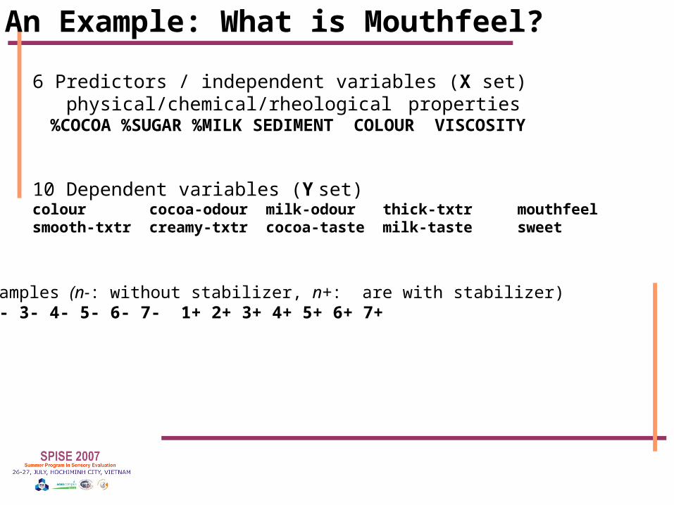
6 Predictors / independent variables (X set) physical/chemical/rheological properties %COCOA %SUGAR %MILK SEDIMENT COLOUR VISCOSITY
10 Dependent variables (Y set)colour cocoa-odour milk-odour thick-txtr mouthfeel smooth-txtr creamy-txtr cocoa-taste milk-taste sweet
14 Samples (n-: without stabilizer, n+: are with stabilizer)1- 2- 3- 4- 5- 6- 7- 1+ 2+ 3+ 4+ 5+ 6+ 7+
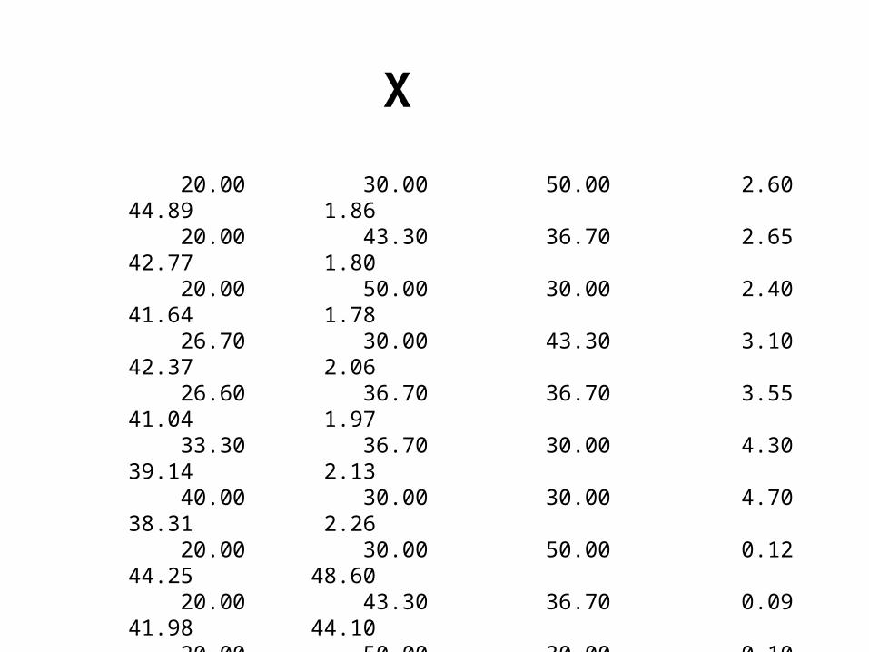
20.00 30.00 50.00 2.60 44.89 1.86 20.00 43.30 36.70 2.65 42.77 1.80 20.00 50.00 30.00 2.40 41.64 1.78 26.70 30.00 43.30 3.10 42.37 2.06 26.60 36.70 36.70 3.55 41.04 1.97 33.30 36.70 30.00 4.30 39.14 2.13 40.00 30.00 30.00 4.70 38.31 2.26 20.00 30.00 50.00 0.12 44.25 48.60 20.00 43.30 36.70 0.09 41.98 44.10 20.00 50.00 30.00 0.10 41.18 43.60 26.70 30.00 43.30 0.10 41.13 47.80 26.60 36.70 36.70 0.10 40.39 50.30 33.30 36.70 30.00 0.10 38.85 51.40 40.00 30.00 30.00 0.09 37.91 54.80
X
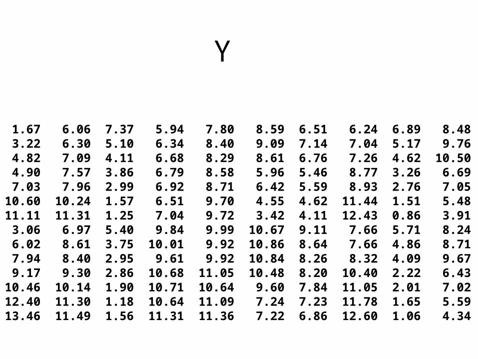
1.67 6.06 7.37 5.94 7.80 8.59 6.51 6.24 6.89 8.48 3.22 6.30 5.10 6.34 8.40 9.09 7.14 7.04 5.17 9.76 4.82 7.09 4.11 6.68 8.29 8.61 6.76 7.26 4.62 10.50 4.90 7.57 3.86 6.79 8.58 5.96 5.46 8.77 3.26 6.69 7.03 7.96 2.99 6.92 8.71 6.42 5.59 8.93 2.76 7.0510.60 10.24 1.57 6.51 9.70 4.55 4.62 11.44 1.51 5.4811.11 11.31 1.25 7.04 9.72 3.42 4.11 12.43 0.86 3.91 3.06 6.97 5.40 9.84 9.99 10.67 9.11 7.66 5.71 8.24 6.02 8.61 3.75 10.01 9.92 10.86 8.64 7.66 4.86 8.71 7.94 8.40 2.95 9.61 9.92 10.84 8.26 8.32 4.09 9.67 9.17 9.30 2.86 10.68 11.05 10.48 8.20 10.40 2.22 6.43 10.46 10.14 1.90 10.71 10.64 9.60 7.84 11.05 2.01 7.0212.40 11.30 1.18 10.64 11.09 7.24 7.23 11.78 1.65 5.5913.46 11.49 1.56 11.31 11.36 7.22 6.86 12.60 1.06 4.34
Y

Why using PLS and PCA and MLR
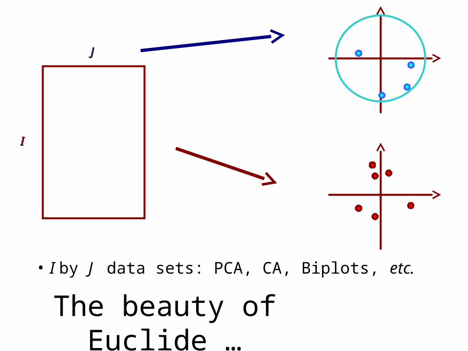
• I by J data sets: PCA, CA, Biplots, etc.
II
JJ
The beauty of Euclide …

• I by J I by 1 (with J << I) data sets: Multiple Regression
II
JJ 11
The beauty of Euclide

• I by J I by K data sets: PLS, CANDIS, etc.
II
JJ KK
The beauty of Euclide
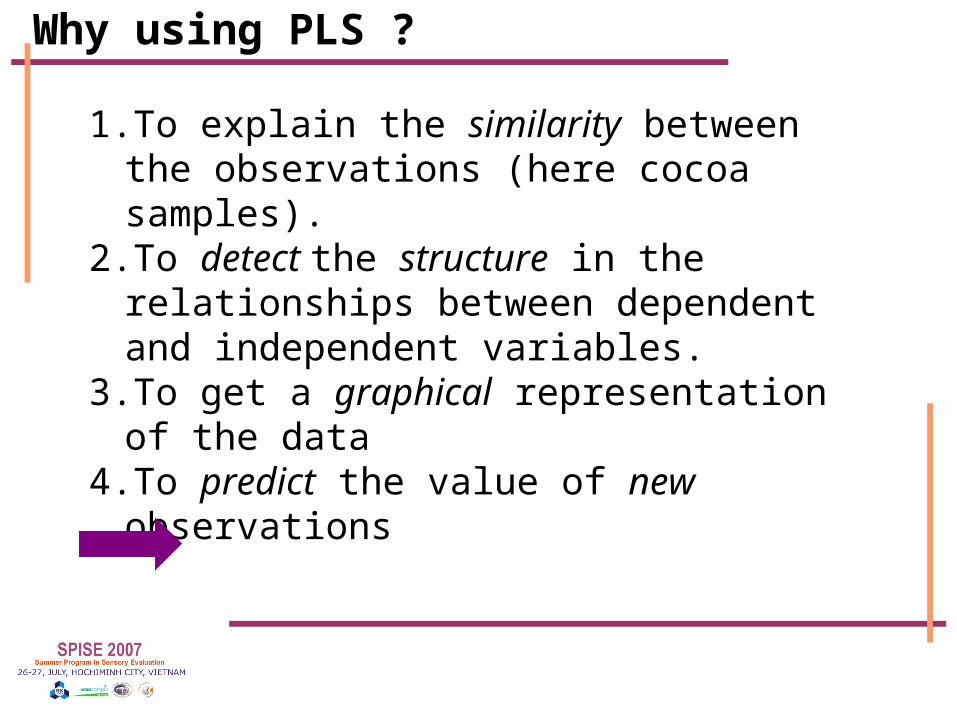
Why using PLS ?
1.To explain the similarity between the observations (here cocoa samples).
2.To detect the structure in the relationships between dependent and independent variables.
3.To get a graphical representation of the data4.To predict the value of new observations

PLS combines features of Principal Component Analysis (PCA) and Multiple Linear Regression (MLR).
Like PCA: PLS extracts factors from X.Like MLR: PLS predicts Y from X
Combine PCA & MLR.PLS extracts factors from X in order to predict Y
What is PLS Regression ?

When to use PLS ?
To analyze two data tables describing the same I observations with J predictors and K dependent variables
1 … j … J
1...i...I
xi,j…...
……
...
IndependentVariables
Obs
erva
tions
1 … k … K
1...i...I
yi,k...............
……
...DependentVariables

General principle of PLS:
1 … j … J1
...i
...I
xij…...
……
...
Predictors XO
bse
rva
tions
t1 … tℓ ... tL1
...i
...I
ti,ℓ…...…
…...
Latent Variables
tℓ= Xwℓ
1 … k … K
1...i...I
yi,k...............
……
...
DependentVariables
Predict
NIPALS
ℓ= tℓ cTY
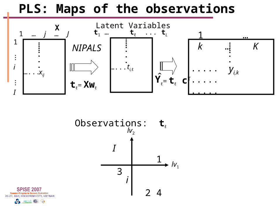
PLS: Maps of the observations
…... xijti,ℓ
t1 … tℓ ... tL
…...
……
...
Latent Variables1 … j … J
1
...i
...I
……
...
X1 … k … K
yi,k...............
……
...
tℓ= Xwℓ
NIPALS
ℓ= tℓ cTY
lv2
lv1
Observations: tℓ
I
i
3
1
2 4

PLS: Maps of the variables
…... xijti,ℓ
t1 … tℓ ... tL
…...
……
...
Latent Variables1 … j … J
1
...i
...I
……
...
X1 … k … K
yi,k...............
……
...
tℓ= Xwℓ
NIPALS
ℓ= tℓ cTY
lv1
lv2
Circle of correlations lv2
lv1
Common map wℓ & cℓ
xx yx
y y y
y y

PLS: Predicting Y from X
…... xijti,ℓ
t1 … tℓ ... tL
…...
……
...
Latent Variables1 … j … J
1
...i
...I
……
...
X1 … k … K
yi,k...............
……
...
tℓ= Xwℓ
NIPALS
ℓ= tℓ cTY
tℓ= Xwℓ & = tℓ cT = XBpls Y Y
Some
Magic
Here!
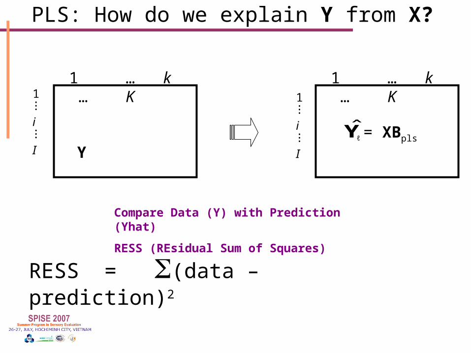
PLS: How do we explain Y from X?
RESS = (data – prediction)2
Compare Data (Y) with Prediction (Yhat)
RESS (REsidual Sum of Squares)
1 … k … K
Y
1...i...I
1 … k … K
ℓ = XBpls Y
1...i...I
1 … k … K
(-1) = X(-1) Bpls Y
2...i...I
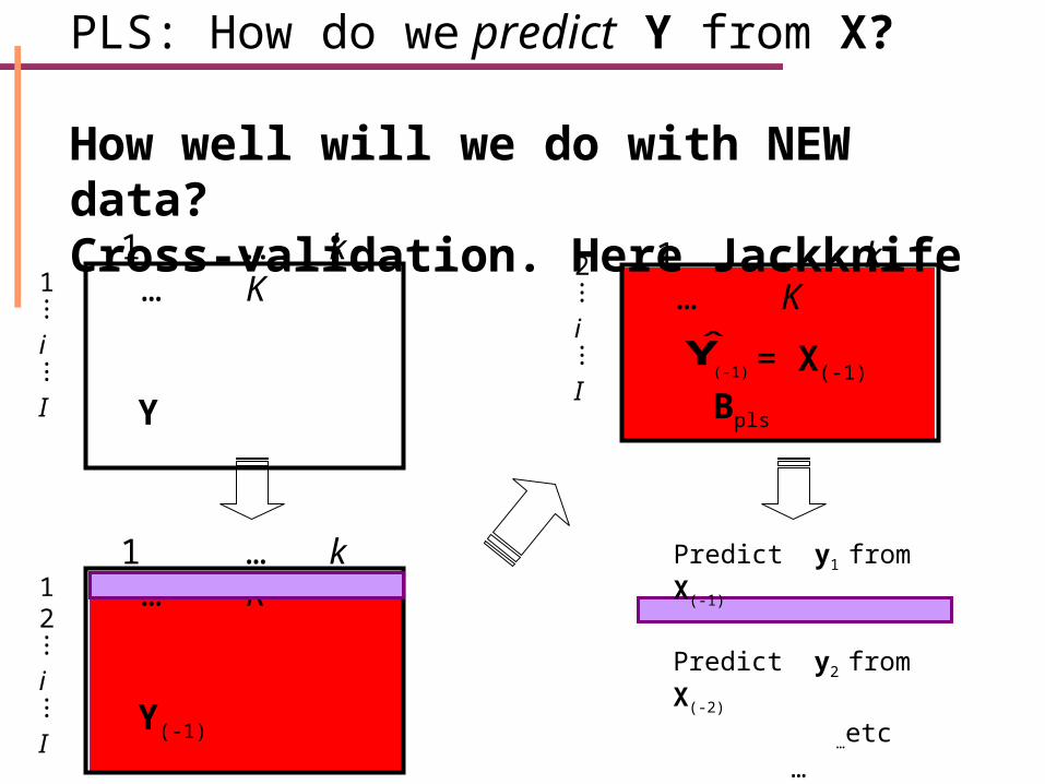
PLS: How do we predict Y from X?
How well will we do with NEW data?Cross-validation. Here Jackknife
1 … k … K
Y
1...i...I
Predict y1 from X(-1) 1 … k … K
Y(-1)
12...i...I
Predict y2 from X(-2)
…etc…
Predict yI from X(-I)
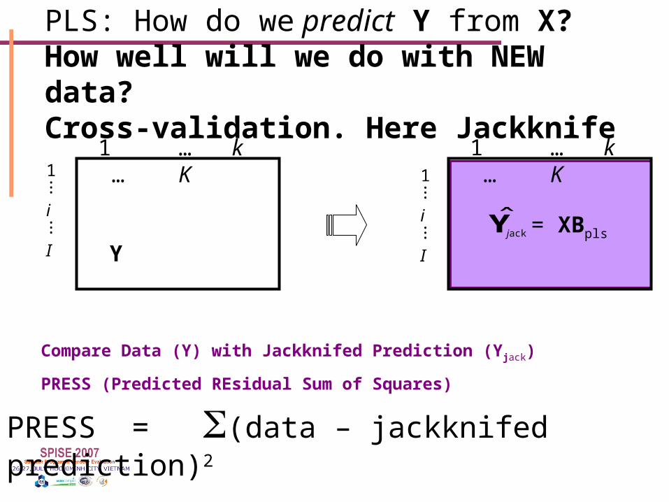
PLS: How do we predict Y from X?How well will we do with NEW data?Cross-validation. Here Jackknife
PRESS = (data – jackknifed prediction)2
Compare Data (Y) with Jackknifed Prediction (Yjack)
PRESS (Predicted REsidual Sum of Squares)
1 … k … K
Y
1...i...I
1 … k … K
jack = XBpls Y
1...i...I
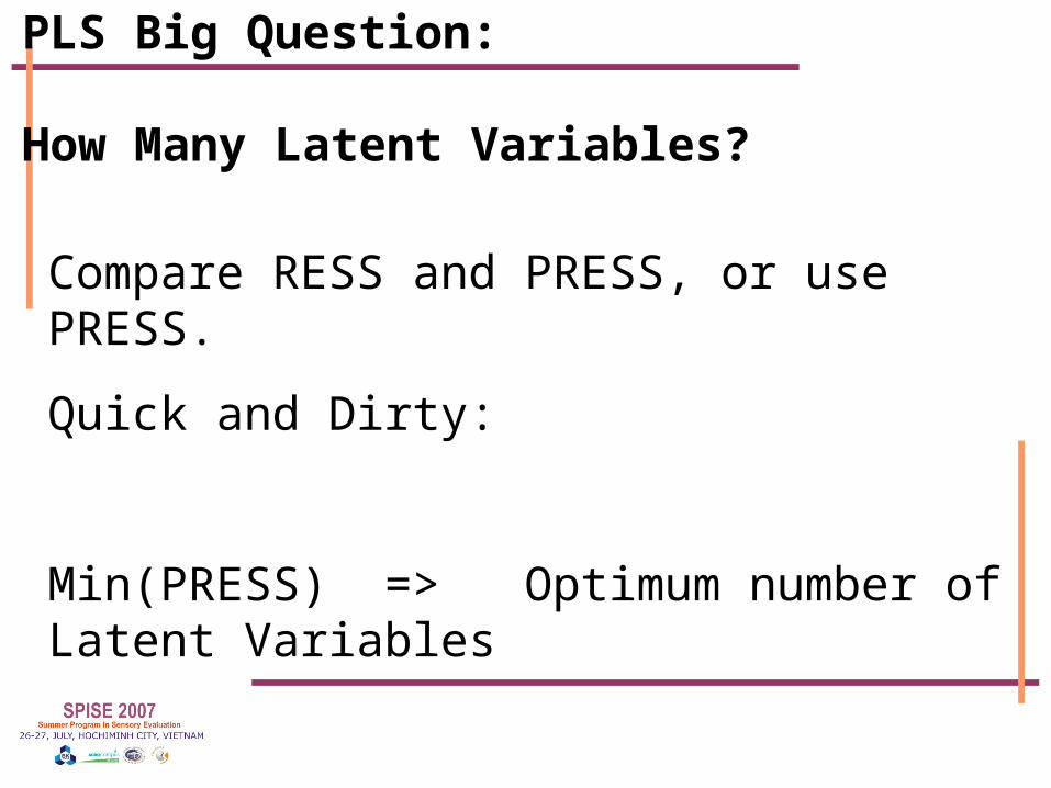
PLS Big Question:
How Many Latent Variables?
Compare RESS and PRESS, or use PRESS.
Quick and Dirty:
Min(PRESS) => Optimum number of Latent Variables
Back to cocoa
Goals: Explain and Predict Sensory (Y) from Physico-Chemical (X)

20.00 30.00 50.00 2.60 44.89 1.86 20.00 43.30 36.70 2.65 42.77 1.80 20.00 50.00 30.00 2.40 41.64 1.78 26.70 30.00 43.30 3.10 42.37 2.06 26.60 36.70 36.70 3.55 41.04 1.97 33.30 36.70 30.00 4.30 39.14 2.13 40.00 30.00 30.00 4.70 38.31 2.26 20.00 30.00 50.00 0.12 44.25 48.60 20.00 43.30 36.70 0.09 41.98 44.10 20.00 50.00 30.00 0.10 41.18 43.60 26.70 30.00 43.30 0.10 41.13 47.80 26.60 36.70 36.70 0.10 40.39 50.30 33.30 36.70 30.00 0.10 38.85 51.40 40.00 30.00 30.00 0.09 37.91 54.80
X

1.67 6.06 7.37 5.94 7.80 8.59 6.51 6.24 6.89 8.48 3.22 6.30 5.10 6.34 8.40 9.09 7.14 7.04 5.17 9.76 4.82 7.09 4.11 6.68 8.29 8.61 6.76 7.26 4.62 10.50 4.90 7.57 3.86 6.79 8.58 5.96 5.46 8.77 3.26 6.69 7.03 7.96 2.99 6.92 8.71 6.42 5.59 8.93 2.76 7.0510.60 10.24 1.57 6.51 9.70 4.55 4.62 11.44 1.51 5.4811.11 11.31 1.25 7.04 9.72 3.42 4.11 12.43 0.86 3.91 3.06 6.97 5.40 9.84 9.99 10.67 9.11 7.66 5.71 8.24 6.02 8.61 3.75 10.01 9.92 10.86 8.64 7.66 4.86 8.71 7.94 8.40 2.95 9.61 9.92 10.84 8.26 8.32 4.09 9.67 9.17 9.30 2.86 10.68 11.05 10.48 8.20 10.40 2.22 6.43 10.46 10.14 1.90 10.71 10.64 9.60 7.84 11.05 2.01 7.0212.40 11.30 1.18 10.64 11.09 7.24 7.23 11.78 1.65 5.5913.46 11.49 1.56 11.31 11.36 7.22 6.86 12.60 1.06 4.34
Y

0 50 10035 40 450 2 430 40 5030 40 5020 30 400
50
10035
40
45024
30
40
5030
40
5020
30
40
Correlation within the X set

010200 510510150 5100 1020510155 10150 5105 10150 10200
102005
105
101505
100
10205
10155
101505
105
10150
1020
Correlation within the Y set
0 50 10035 40 450 2 430 40 5030 40 5020 30 400
102005
105
101505
100
10205
10155
101505
105
10150
1020
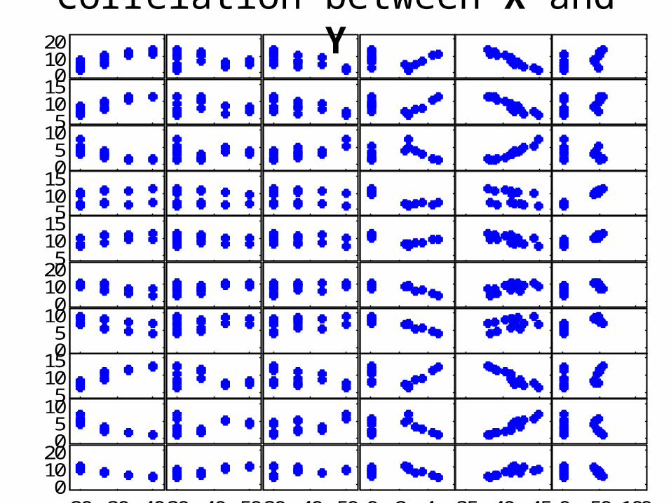
Correlation between X and Y

Show The t (latent) variables• -0.42 -0.19 -0.34 -0.35• -0.25 -0.17 0.22 -0.20• -0.17 -0.14 0.50 -0.22• -0.13 -0.25 -0.26 -0.11• -0.03 -0.27 0.02 0.33• 0.23 -0.36 0.10 0.30• 0.41 -0.42 -0.11 0.06• -0.32 0.27 -0.37 0.04• -0.15 0.27 0.19 0.14• -0.08 0.27 0.46 0.03• 0.01 0.25 -0.29 0.38• 0.07 0.27 -0.02 0.33• 0.32 0.25 0.05 -0.22• 0.51 0.23 -0.16 -0.50
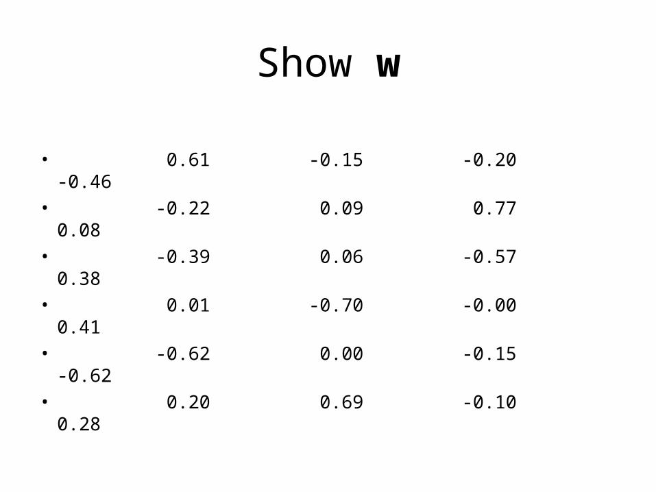
Show w
• 0.61 -0.15 -0.20 -0.46• -0.22 0.09 0.77 0.08• -0.39 0.06 -0.57 0.38• 0.01 -0.70 -0.00 0.41• -0.62 0.00 -0.15 -0.62• 0.20 0.69 -0.10 0.28

Show c
• 0.38 0.12 0.07 0.28• 0.38 0.11 -0.07 0.25• -0.37 -0.05 -0.30 -0.57• 0.15 0.55 -0.18 0.18• 0.27 0.41 -0.25 0.36• -0.23 0.46 0.22 0.10• -0.16 0.53 0.09 0.04• 0.38 0.03 -0.28 0.30• -0.37 0.03 0.07 -0.50• -0.33 0.09 0.81 -0.16
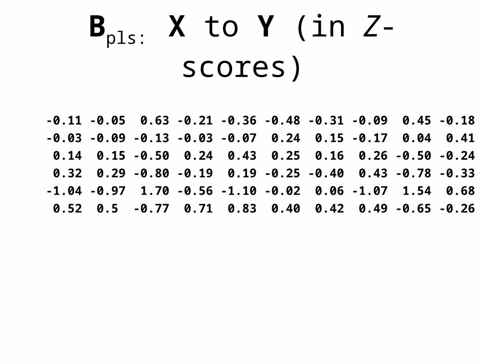
Bpls: X to Y (in Z-scores)
-0.11 -0.05 0.63 -0.21 -0.36 -0.48 -0.31 -0.09 0.45 -0.18
-0.03 -0.09 -0.13 -0.03 -0.07 0.24 0.15 -0.17 0.04 0.41
0.14 0.15 -0.50 0.24 0.43 0.25 0.16 0.26 -0.50 -0.24
0.32 0.29 -0.80 -0.19 0.19 -0.25 -0.40 0.43 -0.78 -0.33
-1.04 -0.97 1.70 -0.56 -1.10 -0.02 0.06 -1.07 1.54 0.68
0.52 0.5 -0.77 0.71 0.83 0.40 0.42 0.49 -0.65 -0.26
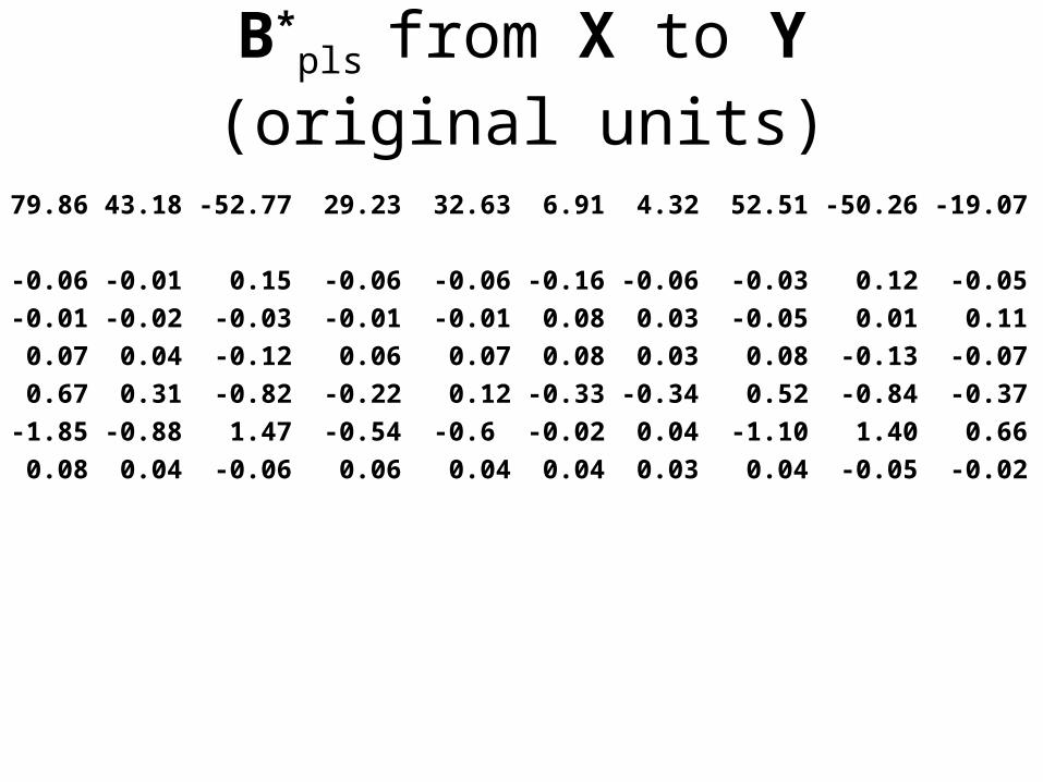
B*pls from X to Y (original units)
79.86 43.18 -52.77 29.23 32.63 6.91 4.32 52.51 -50.26 -19.07
-0.06 -0.01 0.15 -0.06 -0.06 -0.16 -0.06 -0.03 0.12 -0.05
-0.01 -0.02 -0.03 -0.01 -0.01 0.08 0.03 -0.05 0.01 0.11
0.07 0.04 -0.12 0.06 0.07 0.08 0.03 0.08 -0.13 -0.07
0.67 0.31 -0.82 -0.22 0.12 -0.33 -0.34 0.52 -0.84 -0.37
-1.85 -0.88 1.47 -0.54 -0.6 -0.02 0.04 -1.10 1.40 0.66
0.08 0.04 -0.06 0.06 0.04 0.04 0.03 0.04 -0.05 -0.02

Show RESS & PRESS
1 182.39 8505.472 50.86 8318.843 30.28 8292.234 15.69 8286.955 13.00 8299.236 11.91 8309.38
< min PRESS for 4
Keep 4 latent variables
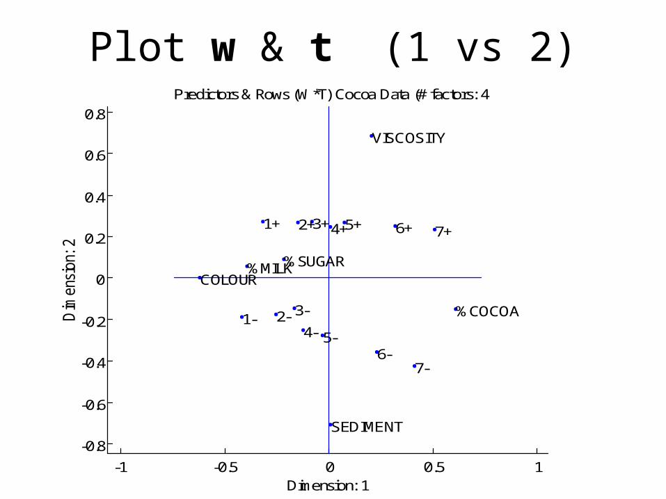
Plot w & t (1 vs 2)
-1 -0.5 0 0.5 1
-0.8
-0.6
-0.4
-0.2
0
0.2
0.4
0.6
0.8
Dimension: 1
Dim
ens
ion:
2
%COCOA
%SUGAR%MILK
SEDIMENT
COLOUR
VISCOSITY
1- 2- 3-
4- 5-6-
7-
1+ 2+3+4+5+ 6+ 7+
Predictors & Rows (W*T) Cocoa Data (# factors: 4
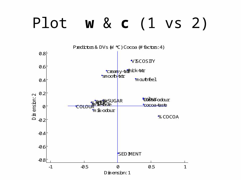
Plot w & c (1 vs 2)
-1 -0.5 0 0.5 1
-0.8
-0.6
-0.4
-0.2
0
0.2
0.4
0.6
0.8
Dimension: 1
Dim
ens
ion:
2
%COCOA
%SUGAR%MILK
SEDIMENT
COLOUR
VISCOSITY
colourcocoa-odour
milk-odour
thick-txtr
mouthfeelsmooth-txtr
creamy-txtr
cocoa-tastemilk-tastesweet
Predictors & DVs (W*C) Cocoa (# factors: 4)
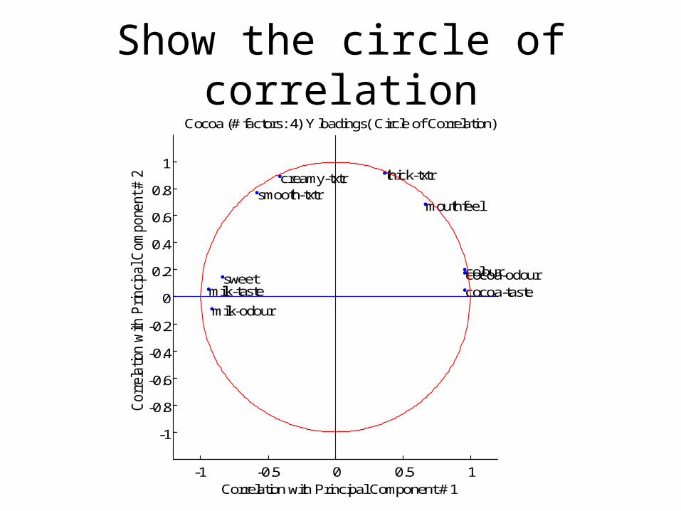
Show the circle of correlation
-1 -0.5 0 0.5 1
-1
-0.8
-0.6
-0.4
-0.2
0
0.2
0.4
0.6
0.8
1
Correlation with Principal Component # 1
Corr
elation
with
Princi
pal C
om
pone
nt # 2
colourcocoa-odour
milk-odour
thick-txtr
mouthfeelsmooth-txtr
creamy-txtr
cocoa-tastemilk-tastesweet
Cocoa (# factors: 4) Y loadings( Circle of Correlation)
Conclusion
• Useful References (contain bibliography):
Abdi (2007, 2003) see www.utd.edu/~herve