planckian distributions in molecular machines, living
TRANSCRIPT
1
Planckian distributions in molecular machines, living cells, and
brains: The wave-particle duality in biomedical sciences
Sungchul Ji*
Abstract --- A new mathematical formula
referred to as the Planckian distribution
equation (PDE) has been found to fit long-
tailed histograms generated in various fields,
including protein folding, single-molecule
enzymology, whole-cell transcriptomics, T-
cell receptor variable region diversity, and
brain neuroscience. PDE can be derived
from the Gaussian distribution law by
applying the simple rule of transforming the
random variable, x, non-linearly, while
keeping the Gaussian y coordinate constant.
There appears to be a common mechanism
underlying all Planckian processes (defined
as those physicochemical processes
generating data that obey PDE), which has
been suggested to be the SID-TEM-TOF
mechanism, the acronym for Signal-Induced
Deactivation of Thermally Excited
Metastable state leading TO Functions. The
universal applicability of PDE to many long-
tailed histograms is attributed to (i) its role
in generating functions and organizations
through goal-directed selection of subsets of
Gaussian processes, and (ii) the wave-
particle duality operating in living systems.
Keywords --- blackbody radiation, fMRI,
Planck distribution equation, single-
molecule enzymology, wave-particle
duality, whole-cell metabolism
*Department of Pharmacology and Toxicology,
Ernest Mario School of Pharmacy, Rutgers
University, Piscataway, N.J.
Proceedings of the International Conference on
Biology and Biomedical Engineering, Vienna, March
15-17, 2015. Pp. 115-137.
I. INTRODUCTION
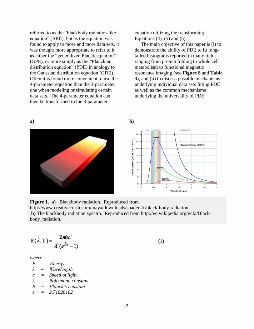
Blackbody radiation refers to the emission
of photons by material objects that
completely absorb photons impinging on
them (hence appearing black). An example
of blackbody radiation is given in Figure 1
a) which shows the emission of different
wavelength light as a function of
temperature. When the light intensity of a
blackbody is measured at a fixed
temperature, the so-called “blackbody
radiation spectrum” is obtained as shown in
Figure 1 b).
M. Planck (1858-1947) succeeded in
deriving the mathematical equation given in
Equation (1) that quantitatively accounted
for the blackbody radiation spectra. The key
to his successful derivation of the so-called
Planck radiation equation was his
assumption that light is emitted or absorbed
by matter in discrete quantities called
“quanta of action,” which led to the birth of
quantum mechanics revolutionizing physics
in the early 20th century [1].
In 2008 [2, Chapter 11], the author
noticed that the single-molecule enzyme-
turnover-time histogram (see the bar graph
in Figure 3 d)) published by Lu et al. [3]
resembled the blackbody radiation spectrum
at 5000 °K (Figure 1 b)). This observation
led me to generalize the Planck radiation
equation, Eq. (1), by replacing its universal
constants and temperature by free
parameters as shown in Equations (2) and
(3), the former having 4 parameters, a, b, A
and B, and the latter 3 parameters, A, B and
C. Depending on the data set to be
analyzed, either the 4- or 3-parameter
equation can be employed. The
“generalized equation” was originally
2
referred to as the “blackbody radiation-like
equation” (BRE), but as the equation was
found to apply to more and more data sets, it
was thought more appropriate to refer to it
as either the “generalized Planck equation”
(GPE), or more simply as the “Planckian
distribution equation” (PDE) in analogy to
the Gaussian distribution equation (GDE).
Often it is found more convenient to use the
4-parameter equation than the 3-parameter
one when modeling or simulating certain
data sets. The 4-parameter equation can
then be transformed to the 3-parameter
equation utilizing the transforming
Equations (4), (5) and (6).
The main objective of this paper is (i) to
demonstrate the ability of PDE to fit long-
tailed histograms reported in many fields,
ranging from protein folding to whole cell
metabolism to functional magnetic
resonance imaging (see Figure 8 and Table
3), and (ii) to discuss possible mechanisms
underlying individual data sets fitting PDE
as well as the common mechanisms
underlying the universality of PDE.
a) b)
Figure 1. a) Blackbody radiation. Reproduced from
http://www.creativecrash.com/maya/downloads/shaders/c/black-body-radiation
b) The blackbody radiation spectra. Reproduced from http://en.wikipedia.org/wiki/Black-
body_radiation.
(1)
where
E = Energy
λ = Wavelength
c = Speed of light
k = Boltzmann constant
h = Planck’s constant
e = 2.71828182
3
[T] = Kelvin (temperature)
[λ] = Meters
h = 6.626.1034 J.s
c = 2.998.108 m/s
k = 1.381.10-23 J/K.
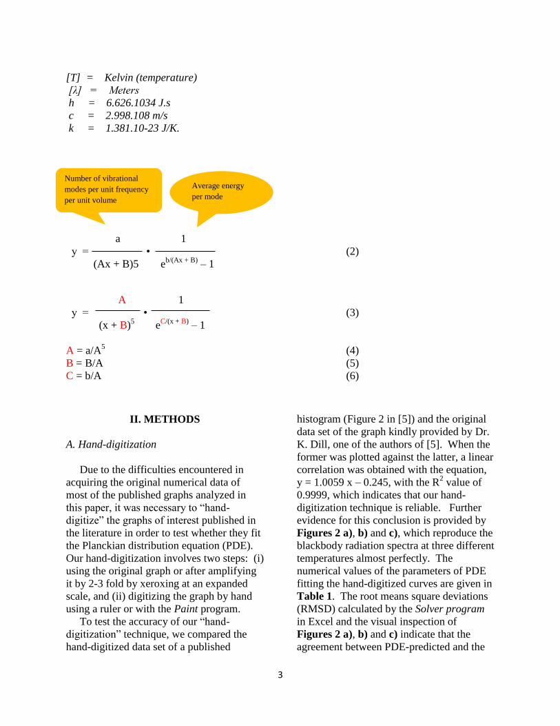
a 1
y = •
(Ax + B)5 eb/(Ax + B)
– 1
(2)
A 1
y = •
(x + B)5
eC/(x + B)
– 1
A = a/A5
B = B/A
C = b/A
(3)
(4)
(5)
(6)
II. METHODS
A. Hand-digitization
Due to the difficulties encountered in
acquiring the original numerical data of
most of the published graphs analyzed in
this paper, it was necessary to “hand-
digitize” the graphs of interest published in
the literature in order to test whether they fit
the Planckian distribution equation (PDE).
Our hand-digitization involves two steps: (i)
using the original graph or after amplifying
it by 2-3 fold by xeroxing at an expanded
scale, and (ii) digitizing the graph by hand
using a ruler or with the Paint program.
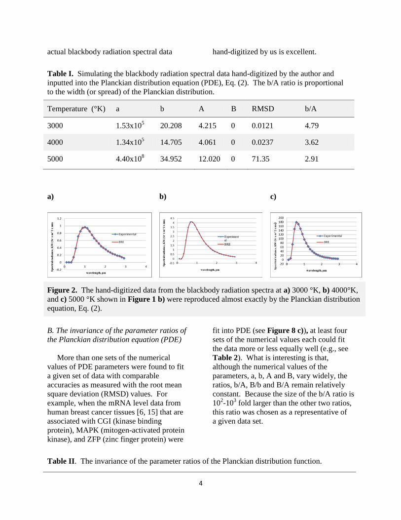
To test the accuracy of our “hand-
digitization” technique, we compared the
hand-digitized data set of a published
histogram (Figure 2 in [5]) and the original
data set of the graph kindly provided by Dr.
K. Dill, one of the authors of [5]. When the
former was plotted against the latter, a linear
correlation was obtained with the equation,
y = 1.0059 x – 0.245, with the R2 value of
0.9999, which indicates that our hand-
digitization technique is reliable. Further
evidence for this conclusion is provided by
Figures 2 a), b) and c), which reproduce the
blackbody radiation spectra at three different
temperatures almost perfectly. The
numerical values of the parameters of PDE
fitting the hand-digitized curves are given in
Table 1. The root means square deviations
(RMSD) calculated by the Solver program
in Excel and the visual inspection of
Figures 2 a), b) and c) indicate that the
agreement between PDE-predicted and the
Number of vibrational
modes per unit frequency per unit volume
Average energy
per mode
4
actual blackbody radiation spectral data hand-digitized by us is excellent.
Table I. Simulating the blackbody radiation spectral data hand-digitized by the author and
inputted into the Planckian distribution equation (PDE), Eq. (2). The b/A ratio is proportional
to the width (or spread) of the Planckian distribution.
Temperature (°K) a b A B RMSD b/A
3000 1.53x10⁵ 20.208 4.215 0 0.0121 4.79
4000 1.34x10⁵ 14.705 4.061 0 0.0237 3.62
5000 4.40x10⁸ 34.952 12.020 0 71.35 2.91
a) b) c)
Figure 2. The hand-digitized data from the blackbody radiation spectra at a) 3000 °K, b) 4000°K,
and c) 5000 °K shown in Figure 1 b) were reproduced almost exactly by the Planckian distribution
equation, Eq. (2).
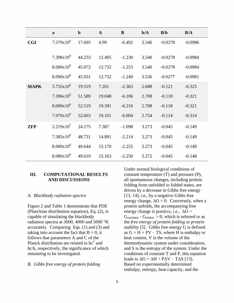
B. The invariance of the parameter ratios of
the Planckian distribution equation (PDE)
More than one sets of the numerical
values of PDE parameters were found to fit
a given set of data with comparable
accuracies as measured with the root mean
square deviation (RMSD) values. For
example, when the mRNA level data from
human breast cancer tissues [6, 15] that are
associated with CGI (kinase binding
protein), MAPK (mitogen-activated protein
kinase), and ZFP (zinc finger protein) were
fit into PDE (see Figure 8 c)), at least four
sets of the numerical values each could fit
the data more or less equally well (e.g., see
Table 2). What is interesting is that,
although the numerical values of the
parameters, a, b, A and B, vary widely, the
ratios, b/A, B/b and B/A remain relatively
constant. Because the size of the b/A ratio is
102-10
3 fold larger than the other two ratios,
this ratio was chosen as a representative of
a given data set.
Table II. The invariance of the parameter ratios of the Planckian distribution function.
5
a b A B b/A B/b B/A
CGI 7.579x10⁶ 17.695 4.99 -0.492 3.546 -0.0278 -0.0986
7.398x10⁸ 44.233 12.495 -1.230 3.540 -0.0278 -0.0984
8.000x10⁸ 45.072 12.732 -1.253 3.540 -0.0278 -0.0984
8.090x10⁸ 45.031 12.732 -1.249 3.536 -0.0277 -0.0981
MAPK 5.755x10⁶ 19.519 7.261 -2.363 2.688 -0.121 -0.325
7.396x10⁸ 51.589 19.048 -6.106 2.708 -0.118 -0.321
8.000x10⁸ 52.519 19.391 -6.216 2.708 -0.118 -0.321
7.970x10⁸ 52.603 19.101 -6.004 2.754 -0.114 -0.314
ZFP 2.219x10⁷ 24.175 7.387 -1.098 3.273 -0.045 -0.149
7.383x10⁸ 48.731 14.891 -2.214 3.273 -0.045 -0.149
8.000x10⁸ 49.644 15.170 -2.255 3.273 -0.045 -0.149
8.080x10⁸ 49.610 15.163 -2.250 3.272 -0.045 -0.148
III. COMPUTATIONAL RESULTS
AND DISCUSSIONS
A. Blackbody radiation spectra
Figure 2 and Table 1 demonstrate that PDE
(Planckian distribution equation), Eq. (2), is
capable of simulating the blackbody
radiation spectra at 3000, 4000 and 5000 °K
accurately. Comparing Eqs. (1) and (3) and
taking into account the fact that B = 0, it
follows that parameters A and C of the
Planck distribution are related to hc2 and
hc/k, respectively, the significance of which
remaining to be investigated.
B. Gibbs free energy of protein folding
Under normal biological conditions of
constant temperature (T) and pressure (P),
all spontaneous changes, including protein
folding from unfolded to folded states, are
driven by a decrease in Gibbs free energy
[13, 14], i.e., by a negative Gibbs free
energy change, ΔG < 0. Conversely, when a
protein unfolds, the accompanying free
energy change is positive, i.e., ΔG =
Gunfolded - Gfolded > 0, which is referred to as
the free energy of protein folding or protein
stability [5]. Gibbs free energy G is defined
as G = H + PV – TS, where H is enthalpy or
heat content, V is the volume of the
thermodynamic system under consideration,
and S is the entropy of the system. Under the
conditions of constant T and P, this equation
leads to ΔG = ΔH + PΔV – TΔS [13].
Based on experimentally determined
enthalpy, entropy, heat capacity, and the
6
length distributions of 4, 3000 proteins from
E. coli, Dill and his coworkers derived a
theoretical equation for protein stability
which generated the experimental curve
shown in Figure 8 a) [5]. As shown, this
theoretical curve is simulated by the
Planckian distribution equation with a great
precision.
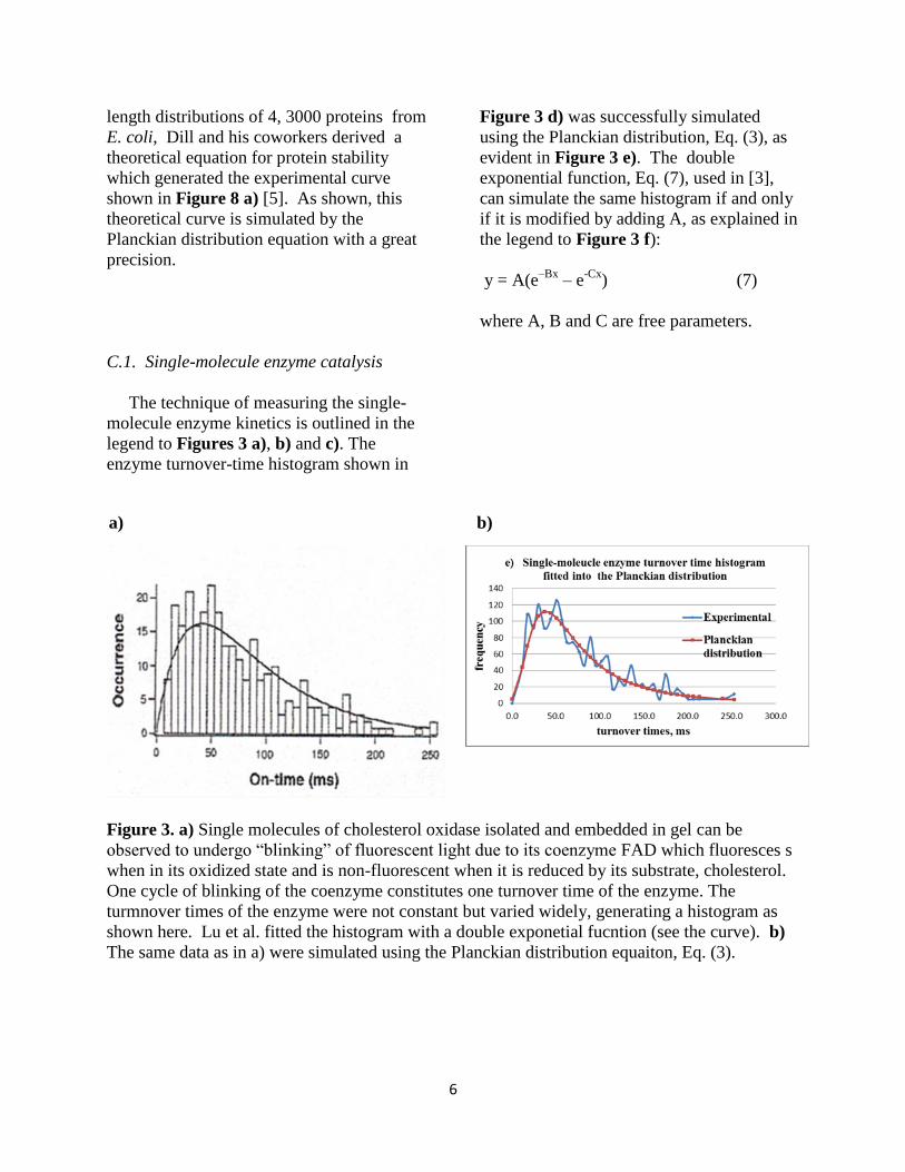
C.1. Single-molecule enzyme catalysis
The technique of measuring the single-
molecule enzyme kinetics is outlined in the
legend to Figures 3 a), b) and c). The
enzyme turnover-time histogram shown in
Figure 3 d) was successfully simulated
using the Planckian distribution, Eq. (3), as
evident in Figure 3 e). The double
exponential function, Eq. (7), used in [3],
can simulate the same histogram if and only
if it is modified by adding A, as explained in
the legend to Figure 3 f):
y = A(e–Bx
– e-Cx
) (7)
where A, B and C are free parameters.
Figure 3. a) Single molecules of cholesterol oxidase isolated and embedded in gel can be
observed to undergo “blinking” of fluorescent light due to its coenzyme FAD which fluoresces s
when in its oxidized state and is non-fluorescent when it is reduced by its substrate, cholesterol.
One cycle of blinking of the coenzyme constitutes one turnover time of the enzyme. The
turmnover times of the enzyme were not constant but varied widely, generating a histogram as
shown here. Lu et al. fitted the histogram with a double exponetial fucntion (see the curve). b)
The same data as in a) were simulated using the Planckian distribution equaiton, Eq. (3).
a) b)
7
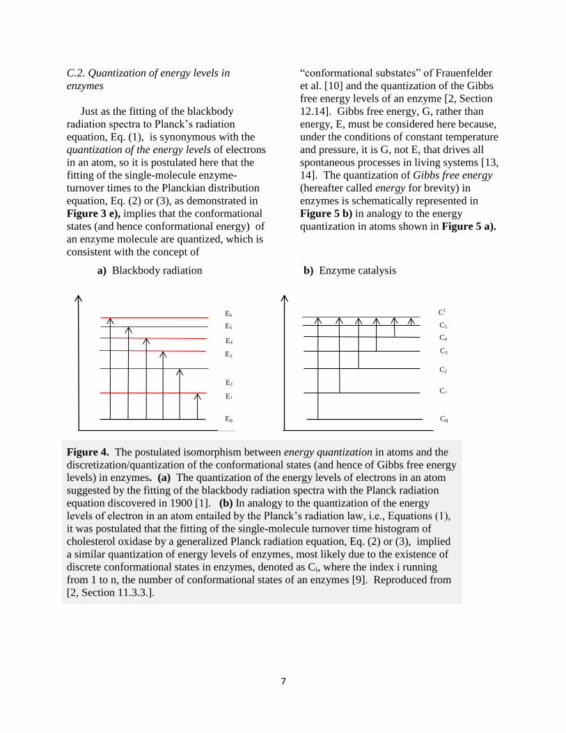
C.2. Quantization of energy levels in
enzymes
Just as the fitting of the blackbody
radiation spectra to Planck’s radiation
equation, Eq. (1), is synonymous with the
quantization of the energy levels of electrons
in an atom, so it is postulated here that the
fitting of the single-molecule enzyme-
turnover times to the Planckian distribution
equation, Eq. (2) or (3), as demonstrated in
Figure 3 e), implies that the conformational
states (and hence conformational energy) of
an enzyme molecule are quantized, which is
consistent with the concept of
“conformational substates” of Frauenfelder
et al. [10] and the quantization of the Gibbs
free energy levels of an enzyme [2, Section
12.14]. Gibbs free energy, G, rather than
energy, E, must be considered here because,
under the conditions of constant temperature
and pressure, it is G, not E, that drives all
spontaneous processes in living systems [13,
14]. The quantization of Gibbs free energy
(hereafter called energy for brevity) in
enzymes is schematically represented in
Figure 5 b) in analogy to the energy
quantization in atoms shown in Figure 5 a).
a) Blackbody radiation b) Enzyme catalysis
Figure 4. The postulated isomorphism between energy quantization in atoms and the
discretization/quantization of the conformational states (and hence of Gibbs free energy
levels) in enzymes. (a) The quantization of the energy levels of electrons in an atom
suggested by the fitting of the blackbody radiation spectra with the Planck radiation
equation discovered in 1900 [1]. (b) In analogy to the quantization of the energy
levels of electron in an atom entailed by the Planck’s radiation law, i.e., Equations (1),
it was postulated that the fitting of the single-molecule turnover time histogram of
cholesterol oxidase by a generalized Planck radiation equation, Eq. (2) or (3), implied
a similar quantization of energy levels of enzymes, most likely due to the existence of
discrete conformational states in enzymes, denoted as Ci, where the index i running
from 1 to n, the number of conformational states of an enzymes [9]. Reproduced from
[2, Section 11.3.3.].
E6
E5
E4
E3
E2
E1
E0
C‡
C5
C4
C3
C2
C1
C0
8
Blackbody radiation involves promoting the
energy levels (vibrational, electronic, or
vibronic) of oscillators from their ground
state E0 to higher energy levels, E1 through
E6. The wavelength of the radiation (or
quantum) absorbed or emitted is given by
ΔE = Ei – E0 = hυ, where Ei is the ith
excited-state energy level, h is the Planck
constant, υ is the frequency, and ΔE is the
energy absorbed when an oscillator is
excited from its ground state to the ith
energy
level. Blackbody radiation results when
electrons transition from a given energy
level to a lower energy level within matter,
e.g., from E1 to E0, or from E2 to E0, etc. [2,
Section 11.3.3].
A single molecule of cholesterol oxidase
is postulated to exist in n different
conformational states (i.e., conformational
substates of Frauenfelder et al. [10]. Each
conformational state (also called a
conformer, or conformational isomer) is
thought to exist in a unique Gibbs free
energy level and carries a set of sequence-
specific conformational strains (called
conformons) [2, Chapters 8 and 11] and can
be excited to a common transition state
(denoted as C‡) by thermal fluctuations (or
Brownian motions), leading to catalysis [2,
Section 11.3.3].
C.3. The Energy Quantization as a Prelude
to Organization
A possible meaning of the energy
quantization invoked in Figure 5 b) to
account for the fitting of the single-molecule
enzyme kinetic data into the Planckian
distribution function, Eq. (2), was proposed
in the following quote reproduced from [2,
p. 111]:
“Quantization (or discretization) may be essential for any organization, since organization
entails selection and selection in turn requires the existence of discrete entities to choose from.
In Sections 11.3.3 and 12.12, experimental evidence is presented that indicates that biological
processes such as single-molecule enzymic activities . . . , whole-cell RNA metabolism . . . and
protein folding . . . are quantized because they all obey mathematical equations similar in form
to the blackbody radiation equation . . . that was discovered by M. Planck in physics in 1900
which led to the emergence of quantum mechanics two and a half decades later. . . .
To make the blackbody radiation data fit a mathematical equation, Planck had to assume that
the product of energy and time called “action” is quantized in the unit later called the Planck
constant, h, which has the numerical value of 6.625x10⁻²⁷
erg∙sec. This quantity seems too small
to have any measurable effects on biological processes which occur in the background of
thermal fluctuations involving energies in the order of kT, where k is the Boltzmann constant,
1.381 x 10⁻¹⁶
erg/degree and T is the absolute temperature. The numerical value of kT is 4.127 x
10-14
ergs at room temperature, T = 298 ºK, which is thirteen orders of ten greater than h. Thus
it appears reasonable to assume that biological processes are quantized in the unit of k rather
than in the unit of h as in physics, which leads me to suggest that
“The Boltzmann constant k is to biology (4-36)
what the Planck constant h is to physics.”
Thus by combining the evidence for the quantization of biological processes provided by Table
4-6 and Statement (4-36), it appears logical to conclude that
9
“Biological processes at the molecular and cellular levels (4-37)
are quantized in the unit of the Boltzmann constant k.”
Elsewhere in [2, p. 110], I also suggested that both information and energy are essential for
organization:
“For the purpose of discussing living processes, it appears sufficient to define ‘organization’
as the nonrandom arrangement of material objects in space and time. I have long felt that both
energy and information are required for any organization, from the Belousov-Zhabotinsky
reaction-diffusion system . . . to the living cell . . . and higher structures. This vague feeling may
now be given a more concrete expression by asserting that ‘organization’ is the complementary
union of information and energy or that information and energy are the complementary aspects
of organization . . . . In other words, the information-energy complementarity may well turn out
to be the elusive physical principle underlying all organizations not only in living systems but
also nonliving systems including the Universe Itself . . . .”
If these speculations turn out to be true in
the future, the fitting of experimental data
into the Planckian distribution equation
displayed in Figure 8 may provide the
empirical basis for integrating energy
quantization, organization, and the
information-energy complementarity into a
coherent theoretical framework previously
referred to as “gnergetics”, defined as the
integrated science (-etics) of information
(gn-) and energy (-erg) [2, pp. 15-18].
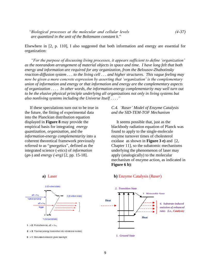
C.4. ‘Raser’ Model of Enzyme Catalysis
and the SID-TEM-TOF Mechanism
It seems possible that, just as the
blackbody radiation equation of Planck was
found to apply to the single-molecule
enzyme turnover times of cholesterol
oxidase as shown in Figure 3 e) and [2,
Chapter 11], so the subatomic mechanisms
underlying the phenomenon of laser may
apply (analogically) to the molecular
mechanism of enzyme action, as indicated in
Figure 6 b):
a) Laser b) Enzyme Catalysis (Raser)
Heat
2. Transition State
1. Ground State
3. Metastable State
4. Substrate-induced
emission of enhanced
rates (i.e., Catalysis)
Heat

10
Figure 5. a) Mechanism underlying Laser (Light Amplification based on the Stimulated
Emission of Radiation). b) Raser (Rate Amplification based on the Substrate-Enhanced reaction
Rates) model of enzyme catalysis, also called the SID-TEM-TOF mechanisms (Stimulus-Induced
Deactivation of Thermally Excited Metastable state leading TO Function).
In the mechanism of laser, the input of
“pumping” photons, hν1, causes the
electrons of the atoms constituting the laser
medium (e.g., ruby crystal) to undergo a
transition from the ground- state energy
level to the excited-state energy level (see
the 1 to 2 arrow in Fig. 6 a)). The excited
state is short-lived, lasting for only about
10-12
seconds, and lose some of its energy
as heat and undergo a transition to a lower
energy level called “metastable” state (see
the 2 to 3 arrow, Figure 6 a)). Sate 3 is
more stable than State 2 but still much more
unstable than the ground state (see 1).
When there are enough number of electrons
in the metastable/excited state (thereby
creating the so-called ”population
inversion”), the arrival of triggering
photons, hν2, induces the de-excitation of
electrons from the metastable excited state
back to the ground state (see the 3 to 1
arrow), accompanied by the emission of
photons identical to the triggering photons,
hν2, but larger in number than the original
triggering photons leading to amplification.
The emitted photons are “coherent” in that
they are identical with respect to (i)
amplitude, (ii) frequency, and (ii) phase.
Unlike electrons in atoms that are all in
the lowest-energy ground state before
absorbing photons, enzymes appear to exist
in different ground states to begin with,
before thermal excitation (i.e., before
absorbing thermal energy), as indicated by
the four solid bars in Figure 6 b), which is
enabled by the quantization of the Gibbs
free energy.
It is possible that, when an enzyme molecule
absorbs enough thermal energies through
Brownian motions, it is excited to the
transition state lasting only for a short period
of time, probably for 10-14
to 10-12
seconds,
the periods of chemical bond vibrations. The
thermally excited enzyme is thought to
undergo a transition to a more stable state
called the “metastable” or “activated” state
lasting probably up to 10-9
seconds. It
appears that the metastable/activated state
can be deactivated in two ways – (i)
spontaneously (as in “spontaneous
emission” in laser), and (ii) induced by
substrate binding (as in “induced emission”).
During spontaneous deactivation of the
active/metastable state of an enzyme, the
excess energy may be released as
uncoordinated random infrared photons,
whereas, during the substrate-induced
deactivation, the excess energy of the
enzyme-substrate complex may be released
in a coordinated manner, resulting in
catalysis, just as the triggering photon-
induced de-activation of population-inverted
electrons in atoms results in the
amplification of emitted photons in laser.
The enzyme catalytic mechanism
depicted in Figure 6 b) may be referred to
as the SID-TEM-TOF mechanism because it
embodies the following three key processes:
(i) Substrate- or Stimuli-Induced
Deactivation in Step 4,
(ii) Thermally Excited Metastable state in
the 1 to 2 and 2 to 3 steps
(iii) leading TO Function i.e., catalysis, in
the 3 to 1 Step.
11
It is here postulated that the SID-TEM-
TOF mechanism underlies many processes
(and/or their records/results) that obey the
Planckian distribution, Eqs. (2) or (3).
D. RNA levels in budding yeast
When glucose is switched to galactose
within a few minutes, budding yeast cells
undergo massive changes in the copy
numbers (from 0 to several hundreds) of its
mRNA molecules encoded by 6,300 genes
over the observational period of hours [11,
12]. Garcia-Martinez et al. [11] measured
the levels of over 5,000 mRNA molecules at
6 time points (0, 5, 120, 360, 450, and 85
minutes) after glucose-galactose shift using
microarrays, generating over 30,000 mRNA
level data oints. Of these data, 2159 mRNA
levels were chosen arbitrarily and grouped
into 250 bins to generate a histogram shown
in Figure 8 b) (see Experimental). As can
be seen in this figure, the histogram fits the
Planckian distribution almost exactly, with
RMSD value of 10.64. The numerical
values of the Planckian distribution
parameters are given in Table 3, Row b).
E. RNA levels in human breast tissues
Perou et al. [6] measured the mRNA
levels of 8,102 genes in the normal cells, the
breast cancer tissues before and after
treating with the anticancer drug,
doxorubicin, in 20 breast cancer patients
using microarrays. Of 8,102 genes, we
analyzed 4,740 genes and their transcripts
from 20 patients. A total of 4,740 x 20 =
94,800 mRNA levels were divided into 60
bins to generate a histogram shown in
Figure 8 c) (see Experimental). Again the
experimental curve fitted the Planckian
distribution equation with great fidelity, the
RMSD value being 368.8. (It should be
pointed out that the magnitude of the RMSD
values depend on the total number of the
points in the data set; the greater the number
of data points, the greater is the RMSD even
if the fit between the experimental and
theoretical curves are comparable by visual
inspection.)
F. Human T-cell receptor gene sequence
diversity
The T-cell receptor consists of two
chains, α and β, and each chain in turn
consists of the transmembrane, constant and
variable regions. The variable regions of T-
cell receptors, called CDR3 (Complement
Determining Region 3), recognize pathogens
and initiate an immune response. The
CDR3 length between conserved residues
ranges from 20 to 80 nucleotides. Murugan
et al. [16] analyzed the nucleotide sequence
data of T-cell beta chain CDR3 regions
obtained from nine human subjects, each
subject generating on average 232,000
unique CDR3 sequences. The germline
DNA encoding the beta chain of human T-
cell receptors has 48 V-genes, 2 D-genes
and 13 J-genes. These gene segments are
recombined via a series of stochastic
recombination mechanisms catalyzed by
appropriate enzymes to generate a large
repertoire of CDR3 sequences. Each CDR3
sequence can be viewed as the result of a
generative event describable by several
random variables, including V-, D- and J-
gene choices.
From the set of observed CDR3
sequences, Murugan et al. [16] was able to
formulate a mathematical equation called
the generative probability function that
predicts the probability of generating CDR3
sequence σ, Pgen(σ). Pgen(σ) is the sum of
the probabilities of all recombination events
12
involved in producing CDR3 sequence σ.
A typical example of the CDR3 sequence
histogram predicted by Pgen(σ) for one
subject is given in Figure 9 d) (see
Experimental). This histogram was obtained
by transforming the original left long-tailed
histogram to the right long-tailed histogram
by replacing - log Pgen(σ) with (30 -
|Pgen(σ)|) , where |Pgen(σ)| is the absolute
value of Pgen(σ). As evident in Figure 8 d),
the agreement between the Pgen(σ)
distribution and the Planckian distribution is
excellent.
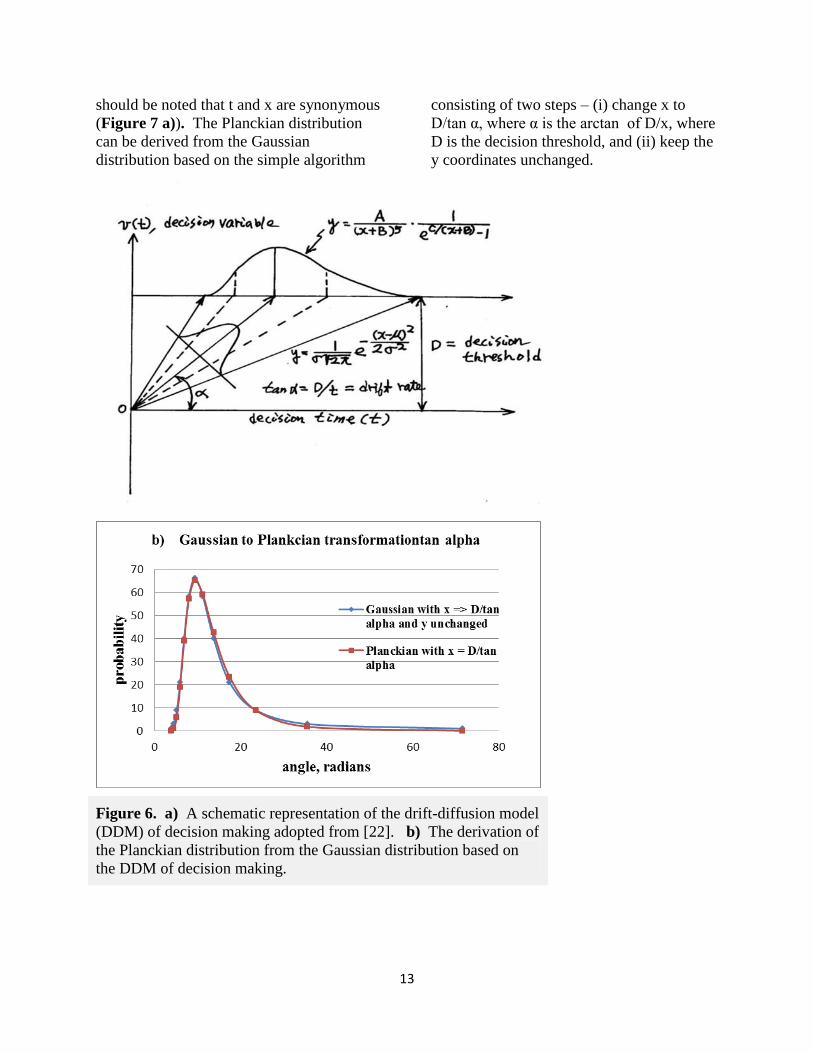
G. Decision-time histogram
The drift-diffusion model (DDM) of
decision-making is a widely employed
theoretical model in behavioral
neurobiology [7, 17, 20, 21, 22]. DDM
accurately reproduces the decision-time
histograms (see Experimental in Figure 8
e)), reflecting the well-known phenomena
[7] that it takes the brain longer to process
more difficult tasks than easier ones. Figure
7 a) depicts the two essential features of
DDM, i.e., (i) the Gaussian-distributed drift
rates (i.e., the rates of evidence
accumulation in the brain), which can be
represented as tan α, where α is the
arctangent of the drift rate, D/t, with D as
the decision threshold (i.e., the level at
which, when reached by accumulating
evidence, a decision is made) and t is the
time when a decision is made, and (ii) the
non-linear relation between the independent
variable of the Gaussian distribution
function and the decision times.
Because of these two features, the
Gaussian-distributed drift rates can produce
a right-long-tailed decision-time histogram
as shown in Figure 7 b), where the right-
long tailed distribution was derived from the
Gaussian distribution based on two
operations: (i) transform the x coordinates of
the Gaussian distribution (obtained by hand-
digitizing the Gaussian curve found at
http://en.wikipedia.org/wiki/Normal_distrib
ution) to D/tan α, and (ii) retain the y
coordinates of the Gaussian distribution
unchanged. As Figurer 7 b) demonstrates,
the Gaussian distribution transformed
according to operations (i) and (ii) above
coincides with the Planckian distribution
based on x, demonstrating that the Planckian
distribution can be derived from the
Gaussian distribution based on DDM, i.e.,
DDM can act as a bridge between the
Gaussian and Planckian distributions.
As shown in Figure 8 e), the
experimentally observed decision-time
histogram was almost perfectly simulated by
the Planckian distribution equation. Just as
random mechanisms can be claimed to
underlie the Gaussian distribution, it may be
claimed that the SID-TEM-TOF (Signal-
Induced Deactivation of Thermally Excited
Metastable state leading TO Function)
mechanism underlies the Planckian
distributions. The SID-TEM-TOF
mechanisms, in turn, can be viewed as the
generalized Raser model of enzyme
catalysis (Figure 6 b)).
It would be convenient to define as the
“Planckian processes” all those processes in
nature that obey the Planckian distribution
law, just as the Gaussian processes can be
defined as those processes that obey the
Gaussian distribution law. Since random
processes are implicated in all Gaussian
processes, so it would be reasonable to
assume that, underlying all Planckian
processes, there exists one or more
mechanisms common to many, if not all,
Planckian processes. One of such common
mechanisms is suggested to be the SID-
TEM-TOF mechanism, i.e., Figure 6 b), or
its equivalent.
The mathematical relation between the
Gaussian and Planckian distributions can be
established based on the drift-diffusion
model (DDM) of decision making [22]. It
13
should be noted that t and x are synonymous
(Figure 7 a)). The Planckian distribution
can be derived from the Gaussian
distribution based on the simple algorithm
consisting of two steps – (i) change x to
D/tan α, where α is the arctan of D/x, where
D is the decision threshold, and (ii) keep the
y coordinates unchanged.
Figure 6. a) A schematic representation of the drift-diffusion model
(DDM) of decision making adopted from [22]. b) The derivation of
the Planckian distribution from the Gaussian distribution based on
the DDM of decision making.
14
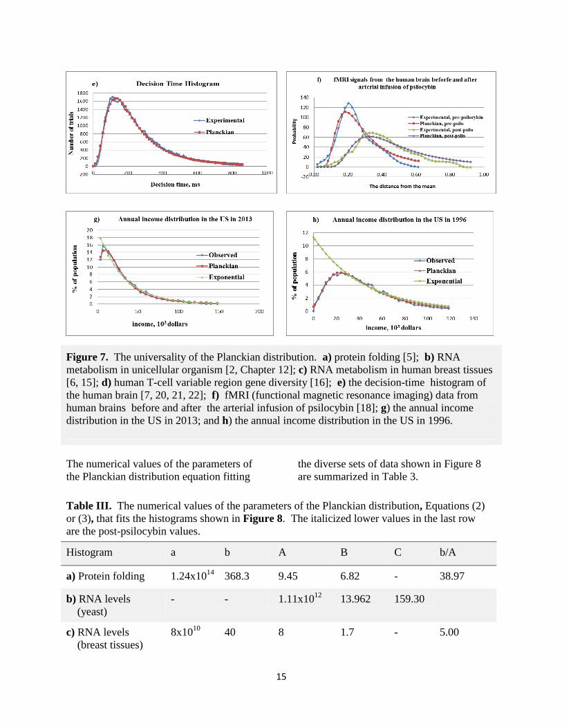
H. fMRI signals from the human brain
before and after psilocybin
The functional magnetic resonance
imaging (fMRI) technique, when applied to
the human brain, allows neuroscientists to
monitor neuronal firing activities in different
regions of the brain noninvasively within
seconds of infusing a psychedelic drug such
as psilocybin. Carhart-Harris et al. [18]
measured the fMRI signals from the brains
of 15 healthy volunteers before and after the
intravenous infusion of psilocybin lasting
for 60 seconds. The subject’s
consciousness, cerebral blood flow (CBF),
and fMRI signals responded within seconds.
CBF values decreased in all regions of the
brain and the subject reported that their
“thoughts wandered freely”. Out of the 9
brains regions examined (2° visual, 1°
visual, motor, DAN, auditory, DMN, R-FP,
L-FP, salience), four regions exhibited
significant changes in their fMRI signals
characterized by increases in the deviations
of the local signals from their mean, i.e., an
increase in variance. By “local” is meant to
indicate brain tissue volume elements
(voxels) measuring a few mm in linear
dimensions. When the distances of the
signals from individual voxels from the
group-mean fMRI signal are calculated and
grouped into bins and their frequencies are
counted, histograms are obtained such as
shown in Figures 8 f), which could be fitted
reasonably well to the Planckian distribution
equation (see Planckian). The numerical
values of the Planckian distribution
equation fitting these two histograms
differed, especially the b/A ratios which
increased from 0.93 to 1.62 by the
psilocybin infusion (see the last two rows in
Table 3).
0
100
200
300
400
0 20 40 60
Nu
mb
er o
f P
ro
tein
s
ΔG, in units of RT
a) Protein folding
Planckian
Experimental
-100
0
100
200
300
0 100 200 300
freq
uen
cy
RNA level bins
b) RNA levels in budding yeast
Experimental
Planckian
15
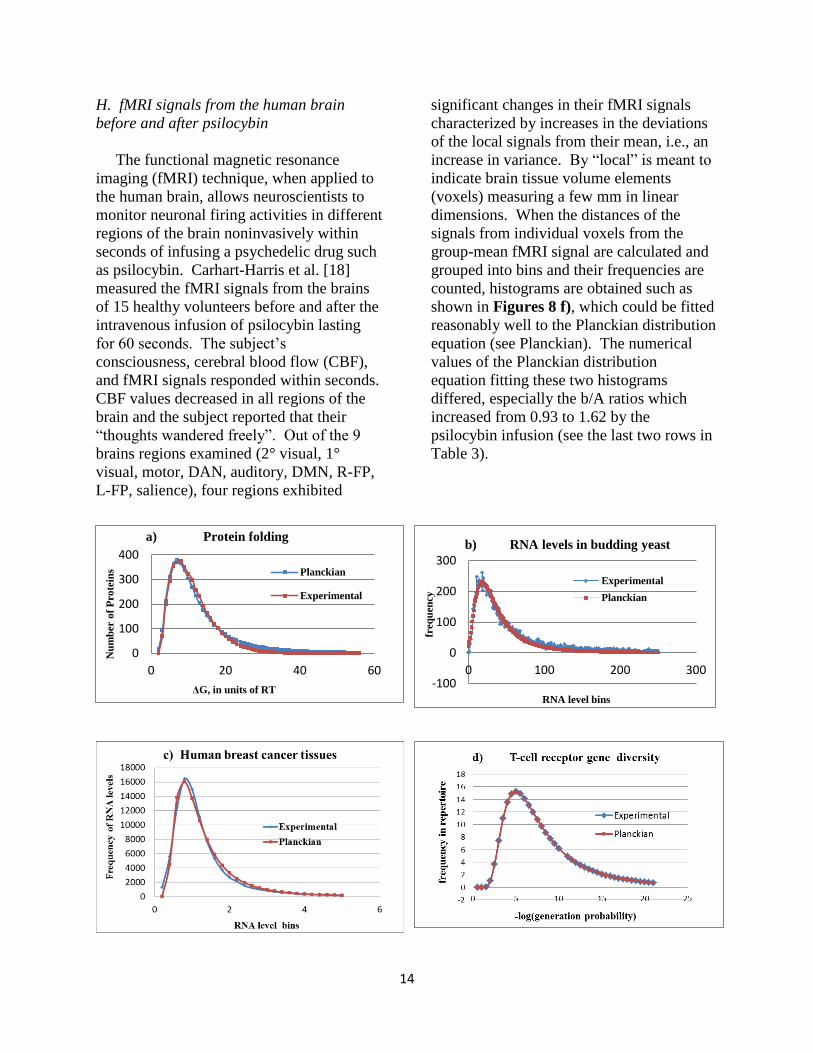
Figure 7. The universality of the Planckian distribution. a) protein folding [5]; b) RNA
metabolism in unicellular organism [2, Chapter 12]; c) RNA metabolism in human breast tissues
[6, 15]; d) human T-cell variable region gene diversity [16]; e) the decision-time histogram of
the human brain [7, 20, 21, 22]; f) fMRI (functional magnetic resonance imaging) data from
human brains before and after the arterial infusion of psilocybin [18]; g) the annual income
distribution in the US in 2013; and h) the annual income distribution in the US in 1996.
The numerical values of the parameters of
the Planckian distribution equation fitting
the diverse sets of data shown in Figure 8
are summarized in Table 3.
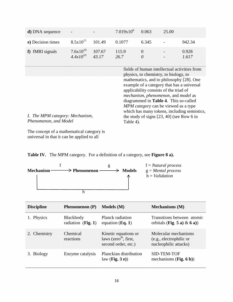
Table III. The numerical values of the parameters of the Planckian distribution, Equations (2)
or (3), that fits the histograms shown in Figure 8. The italicized lower values in the last row
are the post-psilocybin values.
Histogram a b A B C b/A
a) Protein folding 1.24x10¹⁴
368.3 9.45 6.82 - 38.97
b) RNA levels
(yeast)
- - 1.11x10¹²
13.962 159.30
c) RNA levels
(breast tissues)
8x10¹⁰
40 8 1.7 - 5.00
16
d) DNA sequence - - 7.019x10⁶ 0.063 25.00
e) Decision times 8.5x10¹¹
101.49 0.1077 6.345 - 942.34
f) fMRI signals
7.6x10¹⁰
4.4x10¹⁰
107.67
43.17
115.9
26.7
0
0
-
-
0.928
1.617
I. The MPM category: Mechanism,
Phenomenon, and Model
The concept of a mathematical category is
universal in that it can be applied to all
fields of human intellectual activities from
physics, to chemistry, to biology, to
mathematics, and to philosophy [28]. One
example of a category that has a universal
applicability consists of the triad of
mechanism, phenomenon, and model as
diagrammed in Table 4. This so-called
MPM category can be viewed as a type
which has many tokens, including semiotics,
the study of signs [23, 40] (see Row 6 in
Table 4).
Table IV. The MPM category. For a definition of a category, see Figure 8 a).
f g f = Natural process
Mechanism Phenomenon Models g = Mental process
h = Validation
h
Discipline Phenomenon (P) Models (M) Mechanisms (M)
1. Physics Blackbody
radiation (Fig. 1)
Planck radiation
equation (Eq. 1)
Transitions between atomic
orbitals (Fig. 5 a) & 6 a))
2. Chemistry Chemical
reactions
Kinetic equations or
laws (zeroth
, first,
second order, etc.)
Molecular mechanisms
(e.g., electrophilic or
nucleophilic attacks)
3. Biology Enzyme catalysis Planckian distribution
law (Fig. 3 e))
SID-TEM-TOF
mechanisms (Fig. 6 b))
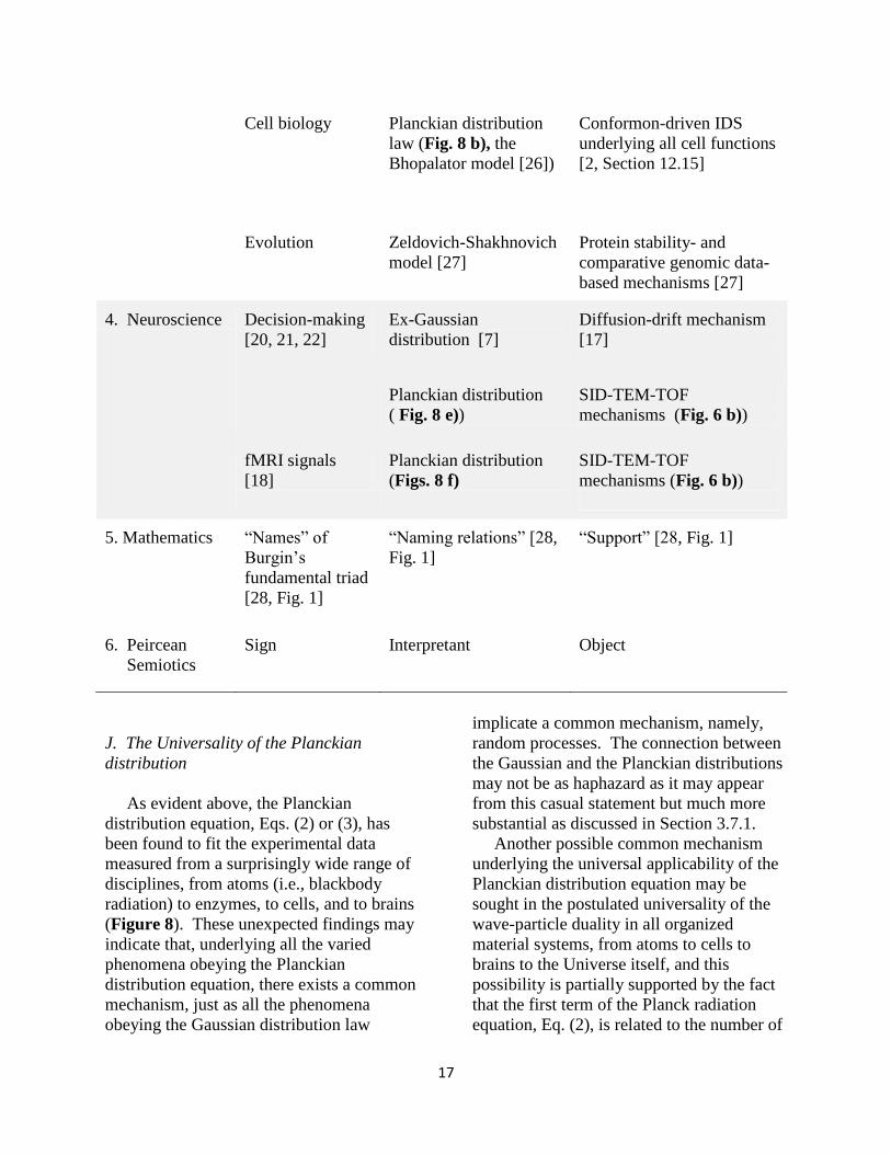
17
Cell biology Planckian distribution
law (Fig. 8 b), the
Bhopalator model [26])
Conformon-driven IDS
underlying all cell functions
[2, Section 12.15]
Evolution Zeldovich-Shakhnovich
model [27]
Protein stability- and
comparative genomic data-
based mechanisms [27]
4. Neuroscience Decision-making
[20, 21, 22]
Ex-Gaussian
distribution [7]
Diffusion-drift mechanism
[17]
Planckian distribution
( Fig. 8 e))
SID-TEM-TOF
mechanisms (Fig. 6 b))
fMRI signals
[18]
Planckian distribution
(Figs. 8 f)
SID-TEM-TOF
mechanisms (Fig. 6 b))
5. Mathematics
“Names” of
Burgin’s
fundamental triad
[28, Fig. 1]
“Naming relations” [28,
Fig. 1]
“Support” [28, Fig. 1]
6. Peircean
Semiotics
Sign Interpretant Object
J. The Universality of the Planckian
distribution
As evident above, the Planckian
distribution equation, Eqs. (2) or (3), has
been found to fit the experimental data
measured from a surprisingly wide range of
disciplines, from atoms (i.e., blackbody
radiation) to enzymes, to cells, and to brains
(Figure 8). These unexpected findings may
indicate that, underlying all the varied
phenomena obeying the Planckian
distribution equation, there exists a common
mechanism, just as all the phenomena
obeying the Gaussian distribution law
implicate a common mechanism, namely,
random processes. The connection between
the Gaussian and the Planckian distributions
may not be as haphazard as it may appear
from this casual statement but much more
substantial as discussed in Section 3.7.1.
Another possible common mechanism
underlying the universal applicability of the
Planckian distribution equation may be
sought in the postulated universality of the
wave-particle duality in all organized
material systems, from atoms to cells to
brains to the Universe itself, and this
possibility is partially supported by the fact
that the first term of the Planck radiation
equation, Eq. (2), is related to the number of
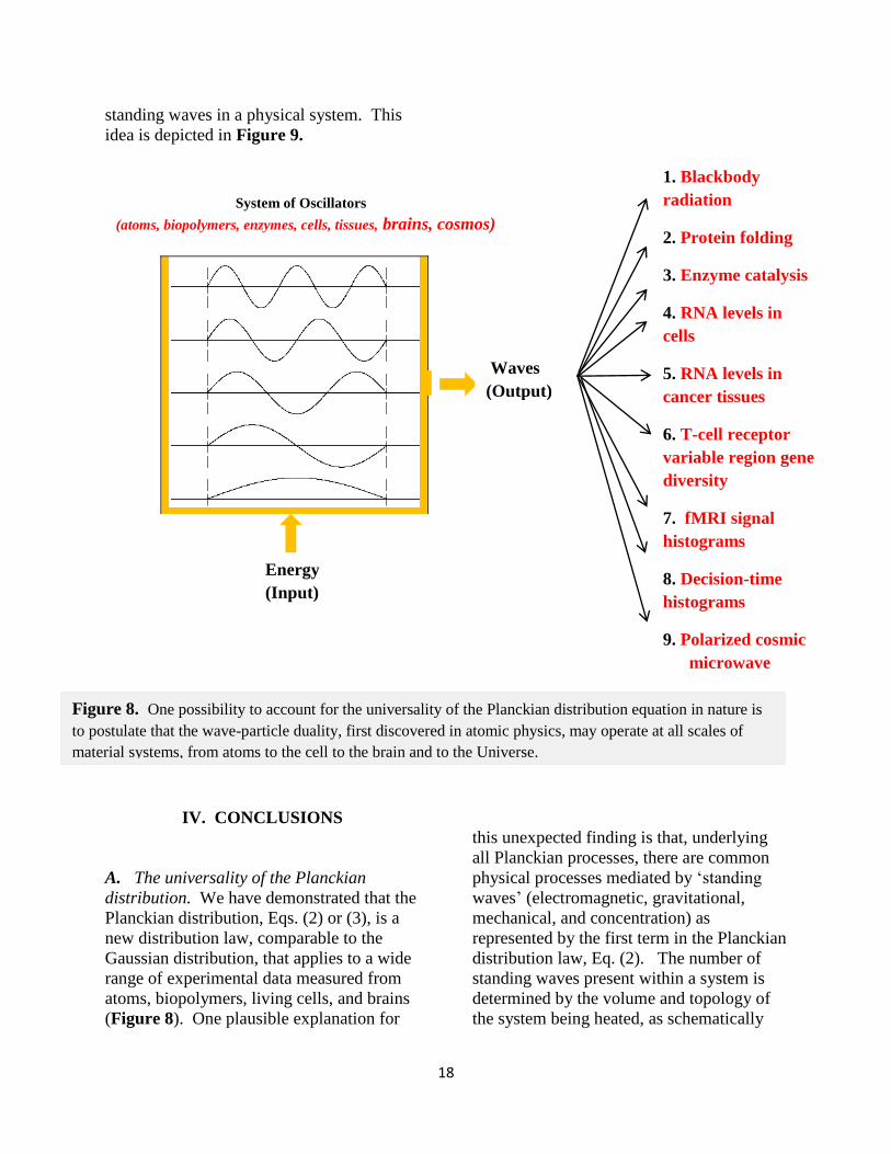
18
standing waves in a physical system. This
idea is depicted in Figure 9.
Energy
(Input)
Waves
(Output)
System of Oscillators
(atoms, biopolymers, enzymes, cells, tissues, brains, cosmos)
1. Blackbody
radiation
2. Protein folding
3. Enzyme catalysis
4. RNA levels in
cells
5. RNA levels in
cancer tissues
6. T-cell receptor
variable region gene
diversity
7. fMRI signal
histograms
8. Decision-time
histograms
9. Polarized cosmic
microwave
background
IV. CONCLUSIONS
A. The universality of the Planckian
distribution. We have demonstrated that the
Planckian distribution, Eqs. (2) or (3), is a
new distribution law, comparable to the
Gaussian distribution, that applies to a wide
range of experimental data measured from
atoms, biopolymers, living cells, and brains
(Figure 8). One plausible explanation for
this unexpected finding is that, underlying
all Planckian processes, there are common
physical processes mediated by ‘standing
waves’ (electromagnetic, gravitational,
mechanical, and concentration) as
represented by the first term in the Planckian
distribution law, Eq. (2). The number of
standing waves present within a system is
determined by the volume and topology of
the system being heated, as schematically
Figure 8. One possibility to account for the universality of the Planckian distribution equation in nature is
to postulate that the wave-particle duality, first discovered in atomic physics, may operate at all scales of
material systems, from atoms to the cell to the brain and to the Universe.
19
represented in Figure 9.
B. Planckian processes as selected
Gaussian processes. Many, if not all,
Planckian processes may derive from the
subset of Gaussian (or random/chaotic)
processes that have been selected because of
their functional roles in physical systems
under given environmental conditions. The
mechanisms enabling such a function-
realizing selection processes may be
identified with the SID-TEM-TOF
mechanism which is in turn dependent on
the Raser model of enzyme catalysis
(Figure 6 b)).
C. The wave-particle duality in biology.
Since (i) the Planckian distribution, Eqs.
(2) or (3), consists of two components – one
related to the number of standing waves per
volume and the other to the average energy
of such oscillatory modes, Eq. (2), (ii) the
wave aspect of the Planck radiation
equation is fundamental in accounting for
not only blackbody radiation spectra but also
subatomic organization of atoms in terms of
atomic orbitals, and (iii) the Planck
distribution applies to both atoms (Figure 2
a), b) and c)) and living systems (Figures
8 a), b), c), d), e), and f)), it appears
logical to infer that the wave aspect of the
wave-particle duality plays a fundamental
role in the behavior of living structures and
processes in biology and medicine. In other
words, it may be impossible for biomedical
scientists to completely account for living
processes, both normal and diseased,
without taking into account of their wave
aspect along with their particle aspect.
D. Science as an irreducible triad of data,
mathematical models, and mechanisms. The
concept of an irreducible triad is basic to the
triadic philosophy of C. S. Peirce [24, pp. 1-
16]. Applying this concept to the definition
of science leads to the conclusion that
science cannot be defined in terms of two or
less of the triad, i.e., data (also known as
measurement), mathematical models, and
physical mechanisms. We may refer to this
philosophical position as the M x M x M or
M3
doctrine of science, where the first M
stands for measurement, the second for
mathematical models, and the third for
physical mechanisms, all of which are
simultaneously required to define science.
The M3 doctrine of science described here
may be viewed as a token or example of the
MPM category defined in Table 4.
ACKNOWLEDGEMENT
I thank my students for their invaluable help
in computing in the Theoretical and
Computational Cell Biology Lab at Rutgers.
My special thanks go to Kenneth So,
Weronika Szafran, Larry Cheng, David Yao,
and Matthew Cheung.
REFERENCES
[1] See Planck’s Law at
http://en.wikipedia.org/wiki/Planck's_law.
[2] S. Ji, Molecular Theory of the Living
Cell: Concepts, Molecular Mechanisms, and
Biomedical Applications, New York:
Springer, 2012.
[3] H. P. Lu, L. Xun, and X. S. Xie,
“Single-Molecule Enzymatic Dynamics,”
Science vol. 282, pp. 1877-1882, 1998.
[4] S. Ji, “Experimental and Theoretical
Evidence for the Energy Quantization in
Molecular Machines and Living Cells, and
the Generalized Planck Equation (GPE),” a
poster presentation at the EMBO/EMBL
Symposium on Molecular Machines:
Lessons from Integrating Structures,
Biophysics and Chemistry, Heidelberg, May
18-21, 2014.
[5] K. A. Dill, K. Ghosh, and J. D. Schmit,
“Physical limits of cells and proteomes,”
20
Proc. Nat. Acad. Sci. USA, vol. 108, no. 44,
pp. 17876-17582, 2011.
[6] C. M. Perou, T. Sorlie, M. B., et al.,
“Molecular portraits of human breast
tumors,” Nature, vol. 406, no. 6797, pp.
747-52, 2000.
[7] R. D. Luce, Response Times: Their
Role in Inferring Elementary Mental
Organization. New York: Oxford
University Press, 1986, Figure 11.4.
[8] H. Frauenfelder, B. H. McMahon, R. H.
Austin, K. Chu, and J. T. Groves, “The role
of structure, energy landscape, dynamics,
and allostery in the enzymatic function of
myoglobin,” Proc. Nat. Acad. Sci. (U.S.),
vol. 98, no. 5, pp. 2370-74, 2001.
[9] J. Garcia-Martinez , A. Aranda, and J. E.
Perez-Ortin, “Genomic Run-On Evaluates
Transcription Rates for all Yeast Genes and
Identifies Gene Regulatory Mechanisms,”
Mol Cell, vol. 15, pp. 303-313, 2004.
[10] S. Ji, A. Chaovalitwongse, N.
Fefferman, W. Yoo, and J. E. Perez-Ortin, “
Mechanism-based Clustering of Genome-
wide mRNA Levels: Roles of Transcription
and Transcript-Degradation Rates,” in
Clustering Challenges in Biological
Networks (S. Butenko, A. Chaovalitwongse,
and P. Pardalos, eds.), Singapore: World
Scientific Publishing Co., 2009, pp. 237-
255.
[11] M. A. Lauffer, “The Significance of
Entropy-Driven Processes in Biological
Systems,” Comments Mol. Cell. Biophys.,
vol. 2, no. 2, pp. 99-109, 1983.
[12] H. B. Callen, Thermodynamics: An
introduction to the physical theories of
equilibrium thermostatics and irreversible
thermodynamics, New York: John Wiley &
Son, Inc., 1985, pp. 90-101.
[13] D. Yao, S. Ji, “Experimental Evidence
for the Cell Force and the Cell Metabolic
Field,” Abstract #31, Ernest Mario School
of Pharmacy Research Day, Great Hall,
Rutgers University, Piscataway, N.J., April
22, 2014.
[14] A. Murugan, T. Mora, A. M. Walczak,
C. G. Callan Jr, “Statistical inference of the
generation probability of T-cell receptors
from sequence repertoires, “ arXiv:
1208.3925v1 [q-bio.QM], 20 Aug 2012.
[15] G. Deco, E. T. Rolls, L. Albantakis, R.
Romo, “Brain mechanisms for perceptual
and reward-related decision-making,”
Progr. Neurobiol., vol. 103, pp. 194–213,
2013.
[16] R. L. Carhart-Harris, R. Leech, P. J.
Hellyer PJ, et al., “The entropic brain: a
theory of consciousness informed by
neuroimaging research with psychedelic
drugs,” Front Human Neurosci, vol. 8, pp.
1-22, 2014. [17] A. Roxin, A. Lederberg,
“Neurobiological Models of Two-choice
Decision Making Can Be Reduced to a One-
Dimensional Nonlinear Diffusion Equation,”
PLoS Computational Biology, vol. 4, no. 3,
pp. 1-13, 2008.
[18] J. Vandekerckhove, F. Tuerlinckx,
“Fitting the Ratcliff diffusion model to
experimental data,” Psychonomic Bulletin
& Review, vol. 14, no. 6, pp. 1011-1026,
2007.
[19] R. Ratcliff, G. McKoon, “The
Diffusion Decision Model,”
http://digitalunion.osu.edu/r2/summer06/we
bb/index.html, 2006.
[20] Arbitrariness of signs. See, for
example,
http://en.wikipedia.org/wiki/Sign_(linguistic
s).
[21] S. Ji, “The Bhopalator – A Molecular
Model of the Living Cell Based on the
Concepts of Conformons and dissipative
Structures,” J. theoret. Biol., vol. 116, pp.
399-426, 1985.
[22] S. Ji S (2012), “The Zeldovich-
Shkhnovich and the MTLC Models of
Evolution,” in Molecular Theory of the
Living Cell: Concepts, Molecular
Mechanisms, and Biomedical
Applications, New York: Springer, pp. 509-
21
519, 2012.
[23] M. Burgin, “Unified Foundations for
Mathematics,”
arXiv:math/0403186[math.LO], 2004.
[24] R. Marty, “76 Definitions of The Sign
by C. S. Peirce,” 2014,
http://www.cspeirce.com/rsources/76defs/76
defs.htm.
[25] C.S. Peirce at
http://en.wikipedia.org/wiki/Charles_Sander
s_Peirce.
[26] Category Theory at
http://en.wikipedia.org/wiki/Category_theor
y