Pivotal Suppliers and Market Power in Experimental Supply Function Competition

Jordi Brandts, Stanley S. Reynolds and Arthur Schram

February 18, 2013

Abstract

In the process of regulatory reform in the electric power industry, the mitigation of market power is one of the basic problems regulators have to deal with. We use experimental data to study the sources of market power with supply function competition, akin to the competition in wholesale electricity markets. An acute form of market power may arise if a supplier is pivotal; that is, if the supplier’s capacity is required in order to meet demand. To be able to isolate the impact of demand and capacity conditions on market power, our treatments vary the distribution of demand levels as well as the amount and symmetry of the allocation of production capacity between different suppliers. We relate our results to a descriptive power index and to the predictions of two alternative models: a supply function equilibrium (SFE) model and a multi-unit auction (MUA) model. We find that pivotal suppliers do indeed exercise their market power in the experiments. We also find that observed behavior is consistent with the range of equilibria of the unrestricted SFE model and inconsistent with the unique equilibria of two refinements of the SFE model and of the MUA model.

Keywords :Market Power,Electric Power Markets, Pivotal Suppliers, Experiments

JEL Classification Codes : C92, D43, L11, L94

Acknowledgements

Financial support by the Spanish Ministerio de Economía y Competitividad (Grant: ECO2011-29847-C02-01), the Generalitat de Catalunya (Grant: 2009 SGR 820), the Antoni Serra Ramoneda Research Chair (UAB-Catalunya Caixa), Consolider-Ingenio 2010 (CSD2006-00016) and the Barcelona GSE Research Support Program is gratefully acknowledged. David Rodríguez provided excellent research assistance. Three anonymous referees and the editor provided very helpful suggestions for improving a previous version of this paper. Remaining errors are ours.

Authors

JordiBrandts Stanley S. Reynolds Arthur Schram

Department of Business Economics UniversitatAutònoma de Barcelona, Institutd’AnàlisiEconòmica(CSIC)

and Barcelona GSE Campus UAB

08193 Bellaterra (Barcelona) Spain

Department of Economics McClelland Hall

Eller College of Management University of Arizona

Tucson, AZ 85721-0108 U.S.A.

CREED Amsterdam School of Economics

Department of Economics and Business

University of Amsterdam Roeterstraat 11

1018 WB Amsterdam The Netherlands

phone +34-93-5814300 Jordi.Brandts@uab.es

phone 1-520-621-6251 Reynolds@eller.arizona.edu

phone +31-20-525.4293 Schram@uva.nl

1

1. Introduction

In the worldwide process of regulatory reform in the electricity industry, the possible

existence of market power is one of the basic problems analysts and policy makers have to

deal with. Field data document the existence of reduced competition due to market power in

some electric power markets (Wolfram 1999; Borenstein et al. 2002). The severe welfare

losses this may cause are a major concern that needs to be addressed to fully assess the

success of the reforms. If non-competitive prices can easily persist in these markets, this

creates the need to find measures to mitigate market power.

Among the features of markets that need to be taken into account in relation to market

power is the presence of one or more pivotal suppliers. In a general sense, a producer can be

considered to be pivotal if, without his capacity, the supply cannot serve the whole demand. It

is important that the issue is not simply one of insufficient total capacity to serve the market

demand, but one of particular producers controlling large enough parts of the capacity. We

will refer to market power due to pivotal suppliers as pivotal power.

Concerns about pivotal power are the basis for some energy policy provisions. Several

organizations that coordinate and regulate wholesale electricity markets in the U.S. – PJM,

Electric Reliability Council of Texas (ERCOT) and California Independent System Operator

(ISO) – employ pivotal supplier screening tests as a trigger for market power mitigation

measures (Reitzes, et al 2007). In addition, the U.S. Federal Energy Regulatory Commission

(FERC) may block a generation company from charging market-based rates for energy if the

company fails a pivotal supplier test for market power. Under the FERC test, a generation

supplier is deemed pivotal, and therefore fails the test, if peak demand cannot be met in the

relevant market without production from the supplier’s capacity.1

A major goal of this paper is to provide evidence from laboratory experiments regarding

the effects of pivotal power. Our design of these experiments and analyses of the data they

generate is guided by a combination of theoretical analysis and tools used in the field. To our

knowledge this is the first experimental study focusing on the specific issue of pivotal power.

A potentially important distinction for policy-makers is the presence of a pivotal supplier vs.

the supplier’s incentive to exercise market power. We examine in the laboratory the extent to

which pivotal suppliers actually exercise market power under varying market conditions. We

1The following quote is from FERC Order No. 697 (2007), pp. 18-19: “The second screen is the pivotal supplier screen, which evaluates the potential of a seller to exercise market power based on uncommitted capacity at the time of the balancing authority area’s annual peak demand. This screen focuses on the seller’s ability to exercise market power unilaterally. It examines whether the market demand can be met absent the seller during peak times. A seller is pivotal if demand cannot be met without some contribution of supply by the seller or its affiliates.”

2

study both the cases where pivotal power is evenly spread among producers and where it is

concentrated in a subset of producers. The first case corresponds more to a situation of tight

market capacity and the second more to a case in which particular firms may have strong

influence on market outcomes, even though market capacity is large. To study more closely

the circumstances under which pivotal power may matter, we also analyze the impact on

market power of a variation in the extent of demand uncertainty.

The use of laboratory experiments makes it possible to implement variations in capacity

distributions with a high degree of control, in order to isolate their effects under conditions

that are strongly ceteris paribus. This control makes the experimental method a useful tool for

studying electric power markets (Rassenti et al. 2002; Staropoli and Jullien 2006). In fact,

experimental research has been very influential in studying and designing mechanisms in a

variety of real world markets, including matching markets (Kagel and Roth, 2000), auctions

(Brunner et al. 2010), and railway competition (Cox et al. 2002). Though pivotal power as

such has not been studied experimentally, previous laboratory experiments do show that

market power is easily exerted in environments that mirror the wholesale electricity market.

Moreover, experiments have been useful for studying how certain market features can

increase or limit market power; demand side bidding (Rassenti, Smith and Wilson 2003) and

forward trading (Brandts, Pezanis-Christou and Schram 2008) have been shown to enhance

competition.

A second important goal of this paper is to provide evidence from laboratory experiments

on the predictive power of two types of theoretical models in settings with and without

pivotal suppliers. One of the advantages of the use of laboratory experiments is that it

facilitates the interplay between theory and data in a way that is not easy to accomplish with

field data. The variations of the conditions in the different treatments of our experiments are

guided by theory and yield specific theoretical predictions for the different cases that can be

directly tested with the experimental data. Our experimental data can, hence, be used to

evaluate theories pertaining to the effect of pivotal suppliers in electric power markets. (See

Falk and Heckman 2009 for a recent methodological discussion of laboratory experiments).

Theoretical analyses of strategic behavior and market power in wholesale electricity

markets have been based on either a multi-unit auction model (Anwar 1999; Fabra von der

Fehr and Harbord 2006), hereafter MUA, or the supply function equilibrium model

(Klemperer and Meyer 1989), hereafter SFE. Both are models of one-shot strategic

interaction. The MUA is a discrete unit model in which each supplier submits price offers for

units of capacity under their control.The SFE assumes a completely divisible good and has

3

been used to study a variety of issues related to electric power markets (Newbery 1998;

Green 1999; Bolle 2001; Baldick et al. 2004; Genc and Reynolds 2011). We explain below

that both the MUA and SFE models can be used to generate equilibrium predictions for

subjects’ behavior in our experiments; moreover, there are differences in equilibrium

predictions for these two models.

A third goal of this paper is to link our analysis of experimental results to the Residual

Supply Index, a measure of pivotal power that has been used in empirical studies with field

data from electric power markets. The Residual Supply Index (hereafter, RSI) measures the

aggregate capacity of all suppliers except the largest as a fraction of total demand. The largest

supplier is pivotal when this index is less than one; lower values of RSI can be interpreted as

yielding more market power for the largest supplier. Rahimi and Sheffrin (2003) find that

higher values of the RSI yield significantly lower price-cost margins for California wholesale

electricity market data for summer peak hours in year 2000. Wolak (2009) develops a

measure of a supplier’s ability to exercise unilateral market power in each half-hour period in

his study of the New Zealand wholesale electricity market. He notes that this ability to

exercise market power is strengthened the greater the probability that the supplier is pivotal

during the period.2 Wolak finds a positive correlation between the average half-hourly firm-

level ability to exercise unilateral market power and half-hourly market prices.

Our experimental design involves three pivotal supplier treatments; two treatments

involve symmetric reductions in sellers’ capacities, and the third involves a reallocation of

sellers’ capacities to create two large, pivotal suppliers. The experimental results allow us to

reject the hypotheses that pivotal power does not matter for these three treatments. Average

market prices are higher in treatments with pivotal power; the way in which average prices

change is intuitive and consistent with the qualitative predictions of the RSI. In contrast to

these effects of capacities, variations in the distribution of demand quantities have smaller

effects on observed market prices. In none of the cases we study does pivotal power lead to

monopoly prices.

Both MUA and SFE models have multiple equilibria for one or more of our experimental

treatment conditions; multiplicity is more pronounced for SFE. Overall, we find that observed

behavior is consistent with the range of equilibria of the unrestricted SFE model and

inconsistent with the equilibria of the MUA model and two refinements of the SFE model. In

2Wolak discusses pivotal suppliers and their significance in the New Zealand wholesale market in Section 3.4 of part 2 of his report. He defines a pivotal supplier as follows: “A supplier that faces a residual demand curve that is positive for all possible positive prices is said to be a pivotal because some of its supply is necessary to serve the market demand regardless of the offer price.” [Wolak (2009), p. 115]

4

treatments without pivotal power, observed prices are on average higher than the (near)

marginal cost level of the MUA equilibrium, though there is a tendency for them to move

towards the competitive MUA prediction. For treatments with pivotal power observed prices

are consistent with the qualitative feature of the SFE that market power caused by a

symmetric reduction in capacity has a stronger effect on prices than market power caused by

an asymmetric distribution of overall high capacity (which is also predicted by the RSI). With

caution one can say that our results suggest that the continued use of the SFE model to study

electric power market as in the work of Niu, Baldick, and Zhu (2005), Hortaçsu and Puller

(2008), Sioshansi and Oren (2007) and Vives (2012) seems warranted.

We also study the best response behavior of our subjects. We compare actual profits to

optimal profits for subjects and compare these results to those from a similar analysis with

field data from the Texas (ERCOT) wholesale power balancing market (Hortacsu and Puller

2008). We find that the behavior we observe in our experiments is closer to best responding

than behavior in the particular field environment we compare our data to.

Our experiments bear some similarity to multi-unit auction experiments reported on in

Sefton and Zhang (2010); these are sales auctions with three buyer subjects, in contrast to our

procurement auctions with four seller subjects. Subjects in their experiments bid on multiple

discrete units, and bids for individual units are from a discrete price grid. The bidding game

corresponding to their experiments has multiple equilibria, with equilibrium prices ranging

from the (common) valuation of bidders (competitive bidding) to a price of zero (tacitly

collusive bidding). Experimental results in Sefton and Zhang are consistent with bids equal to

or slightly below values; they find relatively little evidence of bid shading. This is in contrast

with results in our high-capacity treatments, in which average offers remained well above

marginal cost for some groups. We discuss possible reasons for the differences in

experimental results below.

The remainder of this paper is organized as follows. In the following section, we present

our experimental design and procedures. Specific theoretical predictions are provided in

section 3. The results follow in section 4. Section 5 concludes and discusses the implications

of our findings.

2. Design and Procedures

In the experiment there are 25 rounds each consisting of five periods. The demand is

simulated using a simple box-design (Davis and Holt, 1993). In each of the five periods t in

round r, a perfectly inelastic demand rtd is randomly chosen from the set r

td {dmin,…,dmax}

5

with equal probabilities for each element in the set. In all of our treatments, dmax=35. We

define ldmin/dmax as the load ratio, which is our first treatment variable. All sessions have

either l=4/7 (i.e., dmin=20) or l=6/7 (dmin=30).3 There is a price cap given by pmax=25, i.e. no

units can be traded above this price. Prices and quantities are restricted to integers.

On the supply side there are four firms in each market. Each subject represents one firm.

Each firm j offers a discrete number of units in round r, which will apply to each period t in r.

Any units sold are produced at constant marginal costs c=5.4 Individual supply is limited by

an exogenously enforced maximum capacity maxjs . These determine industry capacity, which

is given by

4

1

maxmax .j

jsS

Our second treatment variable is this industry capacity. This is given by either Smax=48 or

Smax=36. Note that in both cases dmax<Smax, i.e., in all cases industry capacity suffices to

satisfy the maximum demand. Our third treatment variable pertains to the Smax=48 case. We

distinguish between the case where this capacity is distributed evenly across firms (

4,..,1,12max js j ) and the case where there is asymmetric capacity ( 215 ,j,smaxj ,

4319 ,j,smaxj ). For the Smax=36 treatment we only consider the symmetric case (

4,..,1,9max js j ).

Firm j offers units for sale in round r by bidding a discrete ‘supply function’, rjs . This is

a vector of up to maxjs supply prices, sr

jkp , ordered from low to high at which firm j is willing

to sell units: rjs =( sr

js

srj

srj

jppp max,...,, 21 ), with .2,1 kpp sr

jksrjk

5

Subjects can offer fewer than

maxjs units by not entering prices for them. Equivalently, they can offer m< max

js units by

setting .,...,1,26 maxj

srjk smkp 6

The individual supply functions are combined and

supply prices are ordered from low to high to obtain the market supply function for round r,

denoted by sr=( )(),....,1( maxSss rr ), which is a vector of the Smax submitted supply prices

ordered from low to high (if necessary, supplemented with infinite prices for units not

supplied). Finally, a uniform transaction price, rtp , is determined in each period t of r by

comparing rtd to sr: maxmin{ ( ), }.r r r

t tp s d p Note that if max)( pds rt

r , then supply cannot 3 The load ratio affects the theoretically predicted outcomes (cf. section 3). 4 Given our focus on pivotal power, the assumption of constant marginal costs is not restrictive. 5 The “s” superscript on the price variable indicates that the variable is a price offer made by a seller. 6 Units offered at a price above the price cap, pmax=25 will not be sold.

6

satisfy demand at a price below pmax, and k < rtd units are sold, where k is uniquely

determined by sr(k)<25 and sr(k+1)>25.

Finally, the payoffs of firm j in round r, rj , are determined by the uniform prices in each

of the five periods of a round and the marginal costs:

5

1

1 4

r r rj t tj

t

p c q , j ,...,

where rtjq denotes the number of units sold by j in period t of round r.

In the experiment, subjects submit supply functions by entering a price for each possible

unit in a table. To ease the task, the software fills gaps between units priced. For example, if a

subject enters a price of 5 for unit 1 and then 7 for unit 5, then units 2-4 are automatically

priced at 7, though the subject can subsequently change them. In addition, the software does

not allow decreasing prices across units. The subject is free to withhold units from the market

by leaving them unpriced, as long as all subsequent units remain unpriced as well. No supply

price is submitted until the subject finalizes and confirms the complete set. There is no time

limit for submission of the supply functions.

After all four subjects have submitted a supply function, they are aggregated and the

result is confronted with 5 subsequent demand realizations – the 5 periods of a round −

yielding 5 prices. Each realization appears on the subjects’ monitors for 5 seconds. After the

5 periods, the subject can page back and forth between the periods until satisfied. After

everyone has indicated that they are ready the next round commences.

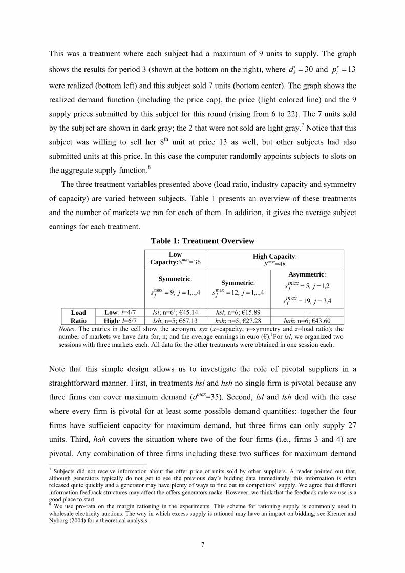
The results of a period appear on the screen graphically and in numbers. Figure 1 shows

an example of the graph a subject could see – the text is in Dutch.

Figure 1: Screenshot of Period Results

Notes. Translation from Dutch: Prijs = Price; Verkocht/Vraag = Sold/Demand; Verkocht door u = Sold by you; Toonperiodes = Show periods.

7

This was a treatment where each subject had a maximum of 9 units to supply. The graph

shows the results for period 3 (shown at the bottom on the right), where 303 td and 13r

tp

were realized (bottom left) and this subject sold 7 units (bottom center). The graph shows the

realized demand function (including the price cap), the price (light colored line) and the 9

supply prices submitted by this subject for this round (rising from 6 to 22). The 7 units sold

by the subject are shown in dark gray; the 2 that were not sold are light gray.7 Notice that this

subject was willing to sell her 8th unit at price 13 as well, but other subjects had also

submitted units at this price. In this case the computer randomly appoints subjects to slots on

the aggregate supply function.8

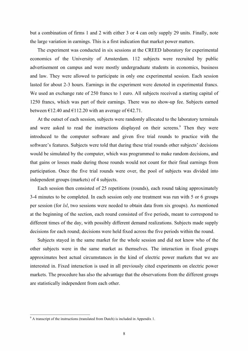
The three treatment variables presented above (load ratio, industry capacity and symmetry

of capacity) are varied between subjects. Table 1 presents an overview of these treatments

and the number of markets we ran for each of them. In addition, it gives the average subject

earnings for each treatment.

Table 1: Treatment Overview

Low

Capacity:Smax=36 High Capacity:

Smax=48

Symmetric:

4,..,1,9max js j

Symmetric:

4,..,1,12max js j

Asymmetric:

215 ,j,smaxj

4319 ,j,smaxj

Load Ratio

Low: l=4/7 lsl; n=61; €45.14 hsl; n=6; €15.89 -- High: l=6/7 lsh; n=5; €67.13 hsh; n=5; €27.28 hah; n=6; €43.60

Notes. The entries in the cell show the acronym, xyz (x=capacity, y=symmetry and z=load ratio); the number of markets we have data for, n; and the average earnings in euro (€).1For lsl, we organized two sessions with three markets each. All data for the other treatments were obtained in one session each.

Note that this simple design allows us to investigate the role of pivotal suppliers in a

straightforward manner. First, in treatments hsl and hsh no single firm is pivotal because any

three firms can cover maximum demand (dmax=35). Second, lsl and lsh deal with the case

where every firm is pivotal for at least some possible demand quantities: together the four

firms have sufficient capacity for maximum demand, but three firms can only supply 27

units. Third, hah covers the situation where two of the four firms (i.e., firms 3 and 4) are

pivotal. Any combination of three firms including these two suffices for maximum demand 7 Subjects did not receive information about the offer price of units sold by other suppliers. A reader pointed out that, although generators typically do not get to see the previous day’s bidding data immediately, this information is often released quite quickly and a generator may have plenty of ways to find out its competitors’ supply. We agree that different information feedback structures may affect the offers generators make. However, we think that the feedback rule we use is a good place to start. 8 We use pro-rata on the margin rationing in the experiments. This scheme for rationing supply is commonly used in wholesale electricity auctions. The way in which excess supply is rationed may have an impact on bidding; see Kremer and Nyborg (2004) for a theoretical analysis.

8

but a combination of firms 1 and 2 with either 3 or 4 can only supply 29 units. Finally, note

the large variation in earnings. This is a first indication that market power matters.

The experiment was conducted in six sessions at the CREED laboratory for experimental

economics of the University of Amsterdam. 112 subjects were recruited by public

advertisement on campus and were mostly undergraduate students in economics, business

and law. They were allowed to participate in only one experimental session. Each session

lasted for about 2-3 hours. Earnings in the experiment were denoted in experimental francs.

We used an exchange rate of 250 francs to 1 euro. All subjects received a starting capital of

1250 francs, which was part of their earnings. There was no show-up fee. Subjects earned

between €12.40 and €112.20 with an average of €42.71.

At the outset of each session, subjects were randomly allocated to the laboratory terminals

and were asked to read the instructions displayed on their screens.9 Then they were

introduced to the computer software and given five trial rounds to practice with the

software’s features. Subjects were told that during these trial rounds other subjects’ decisions

would be simulated by the computer, which was programmed to make random decisions, and

that gains or losses made during those rounds would not count for their final earnings from

participation. Once the five trial rounds were over, the pool of subjects was divided into

independent groups (markets) of 4 subjects.

Each session then consisted of 25 repetitions (rounds), each round taking approximately

3-4 minutes to be completed. In each session only one treatment was run with 5 or 6 groups

per session (for lsl, two sessions were needed to obtain data from six groups). As mentioned

at the beginning of the section, each round consisted of five periods, meant to correspond to

different times of the day, with possibly different demand realizations. Subjects made supply

decisions for each round; decisions were held fixed across the five periods within the round.

Subjects stayed in the same market for the whole session and did not know who of the

other subjects were in the same market as themselves. The interaction in fixed groups

approximates best actual circumstances in the kind of electric power markets that we are

interested in. Fixed interaction is used in all previously cited experiments on electric power

markets. The procedure has also the advantage that the observations from the different groups

are statistically independent from each other.

9 A transcript of the instructions (translated from Dutch) is included in Appendix 1.

9

3. Theoretical Predictions and Hypotheses

As mentioned in the introduction, we center our theoretical analysis on a descriptive index,

the RSI (Residual Supply Index) and two theoretical models, the MUA (multi-unit auction

model) and SFE (supply function equilibrium model). In this section we formulate specific

hypotheses derived from these benchmarks. Our hypotheses will pertain to prices. In

particular, we will use the volume weighted average price (VWAP, hereafter), which is

defined as the monetary value of trades divided by the number of units traded per round. The

VWAP provides a useful way to compare observed prices in experiments to theoretical

predictions. Formally, let be the expected price when d units of output are demanded.

The expected VWAP is defined as,

35

20

( )

[ ]

e

d

d p dP

E d,

Where superscript e denotes expectation and δ is the probability of each possible demand

level.

The RSI is an indicator of market power given by the following expression:

′

where we have used the fact that in our notation seller j=3 has the highest capacity in all

treatments (as does seller j=4). Table 2 shows the range of RSI for each of our treatments, as

well as the midpoint of the interval.

Table 2: RSI

Low Capacity High Capacity: Symmetric: Symmetric: Asymmetric:

Load Ratio

Low [0.71,1.25], 0.98, lsl [1.03,1.80], 1.415, hsl -- High [0.71,0.83], 0.77, lsh [1.03,1,20], 1.115, hsh [0.83,0,97], 0.90, hah

Notes. The first entry in the cell shows the range within which the RSI falls for the various possible demand realizations in the treatment concerned. The second entry shows the midpoint of that interval. The third entry is the treatment acronym defined in table 1.

If no firms are pivotal for any demand quantity, as in high-capacity treatments hsh and hsl,

then the RSI exceeds one in all periods of all rounds; in this case any group of three firms has

enough capacity to meet demand. If the largest firm is pivotal for all demand quantities, as in

treatments lsh and hah, then the RSI is less than one for all periods of all rounds. For

treatment lsl firms are pivotal for low demand quantities but not for high quantities. RSI is

less than one for some periods and greater than one for other periods in treatment lsl. We

expect treatments with higher average values of RSI to have lower market prices.

( )p d

10

The descriptive index is useful but has clear limitations, as it does not propose specific

price levels for the different parameter configurations we analyze. The MUA and the SFE

take us a bit further in this regard. Both models analyze the interaction between firms as a one

shot strategic game, where the strategies consist of supply functions. Of course, the subjects

in our experiment are engaged in a 25-round repeated game, so that the equilibrium

prescriptions do not exactly pertain to the environment we study. However, as in many other

studies the equilibria of the one shot game are relevant benchmarks, particularly given the

known and finite time horizon we use. The central difference between the two models is that

the MUA pertains to discrete production units while the SFE specifies continuously divisible

output.

MUA Predictions

The MUA considers the game as an auction in which each firm j submits a vector of offer

prices, selected from non-negative real numbers, for discrete units of output, .rjs This game is

analyzed in Anwar (1999) and Fabra, et al. (2006). For our parameters, this formulation

yields pure strategy equilibria for treatments hsh, hsl, hah, and lsh; the equilibrium is in

mixed strategies for treatment lsl. Details are given in Appendix 2.

Equilibria for high-capacity treatments hsh and hsl involve market-clearing prices equal

to or slightly above marginal cost (c = 5); the intervals of predicted equilibrium VWAP are

provided in Table 3. The excess capacity present in treatments hsh and hsl provides

incentives for price cutting when offers are above marginal cost. Price cutting incentives are

mitigated to some degree because price offers are restricted to discrete units in the

experiments.10

Pure strategy equilibria of MUA for hah and lsh involve asymmetric strategies, in which

3 firms offer all units at a low price, and the 4th firm (one of the two high-capacity firms for

hah) offers all of its units at 25 (the price cap). The equilibrium price is equal to 25 for all

demand realizations. The firm submitting high-price offers earns lower expected profit than 10The MUA model with continuous price offers provides a simple prediction for these treatments; any pure strategy Nash equilibrium (PSNE) yields market-clearing prices equal to marginal cost (c = 5). This prediction is driven by strong incentives to undercut rivals price offers in the symmetric, high capacity treatments. Our experimental design departs from the continuous price interval assumption by specifying that price offers must be chosen from a set of discrete prices. When price offers are restricted to a set of discrete price offers the incentive to undercut is weakened, since a discrete price cut may involve a significant loss of revenue for infra-marginal units. Indeed, Sefton and Zhang (2010) have an experimental design for a multi-unit sales auction with discrete units and n = 3 bidders for which a PSNE of the one-shot game can sustain collusive bidding, even in a setting in which n – 1 bidders value units above the cost of all of the units available from the seller. Derivation of equilibrium strategies for our procurement auction setting is more complex than for the Sefton and Zhang design since we allow n = 4 subject bidders, and have a larger number of quantity units per subject to bid on and a larger number of discrete prices to choose from.

11

its rivals; the low-price offers of rivals leave the high-price firm with no incentive to reduce

its offers. These equilibria embody maximal exercise of market power; firms extract the

maximum possible surplus in equilibrium.11,12

In treatment lsl firms are pivotal for high demand quantities, but not for low demand

quantities. There are no pure strategy equilibria of the MUA for lsl. Fabra, et al (2006) derive

a mixed strategy equilibrium for the case in which firms are restricted to make a single price

offer for their capacity. However, Anwar (1999) shows that mixing over a single offer is not

an equilibrium when each firm can make distinct offers for multiple units. We are not aware

of analytical results for mixed strategy equilibria of MUA in which each firm can submit

multiple offers. However, we can provide bounds on mixed strategy prices. Our experiment

requires firms to submit offers in discrete price units from the set {5,6,…,25,26}; a unit

offered at 26 will not be accepted and is equivalent to withholding the unit. In lsl, each firm

submits offers for 9 units. A firm’s strategy is a non-decreasing offer schedule for 9 units;

each firm has a finite set of strategies to choose from.13 It is well known that any finite n-

person non-cooperative game has at least one mixed strategy Nash equilibrium. In Appendix

2 we show that expected equilibrium profit for a seller has a positive lower bound. This profit

bound permits us to bound the equilibrium VWAP for treatment lsl: 11.55e

P .

SFE Predictions

The second theoretical approach permits firms to submit continuous supply functions to an

auctioneer. Klemperer and Meyer (1989) formulate and analyze game-theoretic models in

which demand is uncertain and strategies are continuous, non-decreasing supply functions for

infinitely divisible output. A Nash equilibrium for such a game is termed a Supply Function

Equilibrium (SFE). Genc and Reynolds (2011) extend the SFE analysis of Klemperer and

Meyer to permit capacity constraints and supply functions with discontinuities (e.g., step

functions).

The SFE formulation has been used in a number of studies to predict behavior in naturally

occurring wholesale electricity markets (Green 1999; Newbery 1998; Baldick et al. 2004;

11 This effect of the asymmetric distribution of capacities is reminiscent of the price competition environment with capacity constraints studied experimentally by Davis and Holt (1994). With a symmetric distribution of capacity the (pure strategy) equilibrium price is equal to marginal cost, while for a certain asymmetric distribution of the same capacity the equilibrium prices are above marginal cost. 12 Since the pure strategy equilibria for lsh involve strong asymmetries in strategies and payoffs across players, we also compute a lower bound for expected VWAP (reported in Table 3) that is based on necessary conditions for a symmetric mixed strategy equilibrium. 13 The strategy set is finite, but very large. There are 14,307,150 strategies to choose from.

12

Bolle 2001) in which suppliers submit offers for discrete units of output.14 Output is not

infinitely divisible in our experiments either. Each firm (subject) submits offers for between 5

and 19 discrete units of output, depending on the treatment. This permits us to explore

whether or not the SFE model provides useful predictions of behavior in an environment with

discrete units. In addition, our experiments permit us to compare the predictive power of the

SFE model to that of the MUA model in a particular setting.15

Details of the SFE method applied to our parameters are presented in Appendix 3. Here,

we present the main results derived from this theory. The first point to make is that Nash

equilibrium pure strategies of the MUA model are also equilibrium strategies of the SFE

model. Second, the SFE model admits additional pure strategy equilibria compared to the

MUA model.

Consider our high-capacity hsh and hsl treatments. The equilibria for the MUA model

have price equal to marginal cost (or slightly above marginal cost, for discrete prices); a firm

has an incentive to undercut any rival offers that are above marginal cost. However, with

infinitely divisible output, if a firm’s rivals submit smooth upward sloping supply curves then

the firm’s best response is to offer its supply at prices above marginal cost. Klemperer and

Meyer (1989) show that in general there are multiple supply function equilibria and these

equilibria involve non-negative price-cost markups. Supply function equilibria for some of

the treatments are illustrated in Figure 2. For hsh and hsl any aggregate supply function

between (and including) the two bold curves indicated by A and B is consistent with a SFE.16

One way to characterize supply function equilibria is by the equilibrium price they

generate when dmax is realized, i.e., )35(max

r

d

rt sp . As illustrated in Figure 2, the set of SFE

for hsh and hsl is characterized by ]25,5[)35( rs , i.e., the price at maximum demand can lie

anywhere between the competitive price and the highest possible price, which in this case is

the same as the monopoly price.

14The assumption of completely devisable goods yields equilibria where prices are continuous functions of quantity. In real world electricity markets (as in our experiments) prices are discrete step functions, however. Holmberg, Newbery and Ralph (2008) show that under certain conditions such step functions converge to continuous supply functions as the number of steps increases. This provides a justification for approximating step functions with smooth supply functions. 15 Under some market rules, one theory may be much more suitable than the other. If market rules limit firms to submitting offers with one or two steps, then the MUA model seems more appropriate than SFE. Some market rules allow firms to submit upward sloping supply functions. For example, the Southwest Power Pool RTO runs an energy balancing market in which each firm submits multiple price-quantity pairs. This RTO interpolates linearly between pairs to yield a piece-wise linear, upward sloping supply curve for the firm. See: http://www.spp.org/section.asp?group=328&pageID=27. A SFE model would seem more appropriate than a MUA model for such market rules. 16 We refer to a SFE in which the aggregate supply function is differentiable over the range of possible demand quantities as a smooth SFE. For example, supply function equilibria associated with aggregate supply functions labeled A and C in figure 2 are smooth.

13

Figure 2: Aggregate Supply Functions for SFE

Notes. The curves show possible aggregate supply curves for smooth supply function equilibria. The vertical dashed line at Q=35 indicates maximum demand dmax. For hsh and hsl, any curve between A and B constitutes a SFE. For lsh and lsl the set of aggregate supply curves for smooth SFE is reduced to the curves between A and some curve C, above curve B.

Consider now treatments lsh and lsl for which each firm is pivotal; other firms cannot fully

compensate if one firm withholds units. The market power induced in these treatments has as

a consequence that supply functions at or near marginal cost for all units for all firms are not

equilibrium strategies. In fact only the aggregate supply functions between some function C

(above B) and A are SFE for these low capacity treatments (cf. figure 2). More specifically,

for lsh, functions characterized by ]25,21[)35( rs are SFE and for lsl this holds for functions

with ]25,18[)35( rs .

For lsh we have to also consider non-smooth SFE. If one allows firms to submit non-

smooth step-function supply functions (formally, right-continuous functions of price) then the

asymmetric equilibria of the MUA with price equal to 25, in which 3 firms offer all units at a

low price and the 4th firm offers all of its units at 25 are also SFE for treatment lsh (but not

for any of the other treatments with symmetric capacity distribution).

For treatment hah the asymmetric equilibria of the MUA, with one of the two high-

capacity firms bidding in all units at a price of 25 (yielding price equal to 25 for all demand

realizations), are also supply function equilibria. There are additional supply function

equilibria for treatment hah with prices below the price cap. In these equilibria, low-capacity

firms offer all units at a low price and high-capacity firms have upward sloping (in fact,

linear) supply functions, which are between supply curves A and B in Figure 3;

]25,9.11[)35( rs for these equilibria.

0

5

10

15

20

25

0 2 4 6 8 10 12 14 16 18 20 22 24 26 28 30 32 34

Pri

ce

Q

A

B

C

14

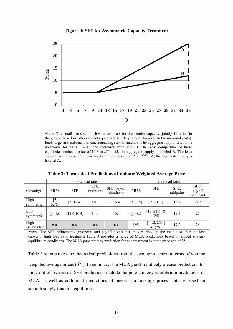
Figure 3: SFE for Asymmetric Capacity Treatment

Notes. The small firms submit low price offers for their entire capacity, jointly 10 units (in the graph, these low offers are set equal to 5, but they may be larger than the marginal costs). Each large firm submits a linear, increasing supply function. The aggregate supply function is horizontal for units 1 – 10 and increases after unit 10. The most competitive of these equilibria reaches a price of 11.9 at dmax =35; the aggregate supply is labeled B. The least competitive of these equilibria reaches the price cap of 25 at dmax =35; the aggregate supply is labeled A.

Table 3: Theoretical Predictions of Volume Weighted Average Price

low load ratio high load ratio

Capacity: MUA SFE SFE:

midpoint SFE: payoff

dominant MUA

SFE

SFE: midpoint

SFE: payoff

dominant High symmetric

[5, 5.75]

[5, 16.4] 10.7 16.4 [5, 7.5] [5, 21.3] 13.2 21.3

Low symmetric

> 11.6 [12.4,16.4] 14.4 16.4 > 18.5 [18, 21.3] &

{25} 19.7 25

High asymmetric

n.a. n.a. n.a n.a {25} [11.2, 23.1]

& {25} 17.2 25

Notes. The SFE refinements (midpoint and payoff dominant) are described in the main text. For the low capacity, high load ratio treatment Table 3 provides a range of MUA predictions based on mixed strategy equilibrium conditions. The MUA pure strategy prediction for this treatment is at the price cap of 25.

Table 3 summarizes the theoretical predictions from the two approaches in terms of volume

weighted average prices (e

P ). In summary, the MUA yields relatively precise predictions for

three out of five cases. SFE predictions include the pure strategy equilibrium predictions of

MUA, as well as additional predictions of intervals of average prices that are based on

smooth supply function equilibria.

0

5

10

15

20

25

1 3 5 7 9 11 13 15 17 19 21 23 25 27 29 31 33 35

Pri

ce

Q

A

B

15

We will also apply two refinements to SFE and investigate how well they organize the

data we observe. First, the ‘midpoint equilibrium’ selects the mean SFE in the range of

symmetric SFE. This is an easy heuristic that attempts to predict average behavior across

markets, assuming that distinct SFE occur with more or less equal probability. Second, the

‘payoff-dominant’ equilibrium is the SFE with the highest VWAP. This has the intuitive

appeal of being best for the players concerned. Both refinements are given in table 3.17

We will use these theoretical predictions to organize our data on volume-weighted-

average prices in several ways. We will study whether observed prices remain within the

interval prescribed by the SFE and, if so, whether they are well approximated by the more

extreme predictions of the SFE refinements or the MUA model, all shown in table 3.

In addition, we will take a more qualitative look at the data and test a set of formal

hypotheses about the comparative static effects that the results in table 3 predict for our

treatment variables. The null hypothesis we use as a benchmark stems from the naive view

that prices should not be expected to differ across treatments, since in all our treatments total

capacity is sufficient to serve the maximum demand. The distinct alternative hypotheses are

based on both the midpoint values of the RSI (table 2) and the predictions that have been

derived using MUA and the two SFE refinements (table 3). The comparisons we perform

pertain to the distinguished treatment variations of total capacity, capacity distribution and

demand load ratio and to the direct comparison of the two ways in which pivotal power is

present in our design.

In the following hypotheses, xP stands for the volume weighted average price in

treatment x. The first two hypotheses refer to the symmetric reduction of capacity, with a

high and low demand load ratio respectively:

1. With a high load ratio, the presence of pivotal firms, due to symmetrically distributed

low total capacity, increases average prices (predicted by RSI, MUA and both SFE

refinements). Formally:

H10: lshhsh PP vs. H11: lshhsh PP

17Alternatively, one may think that the set of SFE equilibria could be refined by a restriction to linear supply functions (as demonstrated by Klemperer and Meyer 1989). This refinement only works with linear, downward sloping demand and linear marginal cost, however. In our environment such an approach does not refine the set of SFE equilibria.

16

2. With a low load ratio, market power caused by a symmetric reduction in capacity

causes an increase in average prices (predicted by RSI, MUA and the midpoint SFE

refinement). Formally:

H20: lslhsl PP vs. H21: lslhsl PP

The next hypothesis refers to the change in distribution of the high total capacity level for the

high demand load ratio.

3. With a high load ratio, the presence of pivotal firms, due to asymmetrically

distributed high total capacity, increases average prices (predicted by RSI, MUA and

both SFE refinements). Formally:

H30: hahhsh PP vs. H31: hahhsh PP

The next hypothesis refers to the two ways in which pivotal power can appear.

4. With ahigh load ratio, market power caused by a symmetric reduction in capacity has

a stronger effect on average prices than market power caused by asymmetry

(predicted by RSI and midpoint-refined SFE). Formally18:

H40: hahlsh PP vs. H41: hahlsh PP

The two remaining pair-wise comparisons pertain to the impact of changing the load ratio.

5. With a high symmetric capacity, the change from a low to a high load ratio yields

higher prices (predicted by RSI and both SFE refinements). Formally:

H50: hslhsh PP vs. H51: hslhsh PP

6. With a low symmetric capacity, the change from a low to a high load ratio leads to

higher prices (predicted by RSI, MUA and both SFE refinements). Formally:

H60: lsllsh PP vs. H61: lsllsh PP

18 The RSI predicts a shift simply because the aggregate capacity that is left after a pivotal supplier withdraws his capacity from the total is smaller under lsh than under hah. The midpoint-SFE picks this up; some of the lower prices that are equilibrium for the hah treatment are not part of the equilibria for lsh. In contrast, the MUA model and the payoff-dominant SFE do not suggest a difference between these two cases; both ways of introducing pivotal power lead to the same (asymmetric) equilibrium with the highest possible price.

17

Observe that both the RSI and the midpoint SFE refinement prescribe a directional shift for

all the cases we consider. The prescriptions of the MUA and of the payoff-dominant SFE do

not change for two of the parameter changes.

4. Results

We start with a general qualitative overview of the supply functions submitted by our

subjects. This is followed by an analysis of the aggregate supply functions. We then present

data on average volume weighted average prices, compare them with the equilibrium

predictions and formally test our hypotheses H1-H6. In the latter part of the section we

analyze individual best responses and assess the theoretical predictions of the two models.

When submitting their individual supply functions, subjects typically submitted all units

that they had available. In the low capacity treatments (where each subject had a capacity of 9

units) on average 8.9 units were offered at a price lower than or equal to pmax(=25). In the

symmetric high capacity cases (12 units each) on average 11.7 units were offered. In the

asymmetric treatment hah (two firms with 5 units and two with 19) the low capacity firms

always offered all units whereas the firms with high capacity on average offered 18.6 out of

19 units at a price lower than or equal to 25. This is an indication that attempts to exert

market power were done by offering units at high prices, not by withholding them

altogether.19

Figure 4 gives the average aggregate supply function per treatment, distinguishing

between the low load ratio and high load ratio cases. In both panels the ranking of the

functions, in relation to the load ratio, is the same. The highest prices are asked for the low

capacity treatments lsh and lsl and the lowest for the symmetric high capacity cases hsh and

hsl. The supply function for the asymmetric capacity case lies somewhere in between, in the

top panel.

Note that the average supply function for hah combines units supplied by small and large

firms. Figure 5 separates the two.20 The figure shows that the ten units of the small firms are

offered at higher prices than the first units of large firms. In equilibrium, all units offered by

the small firms are (on average) sold for any demand realization (which is between 30 and 35

in this treatment), however, because all are within the first 29 units of the aggregate supply

19 Across all treatments, in 82.2% of the rounds the aggregate supply function offered the maximum total capacity at prices lower than or equal to 25. 20We are grateful to an anonymous referee for suggesting this analysis.

18

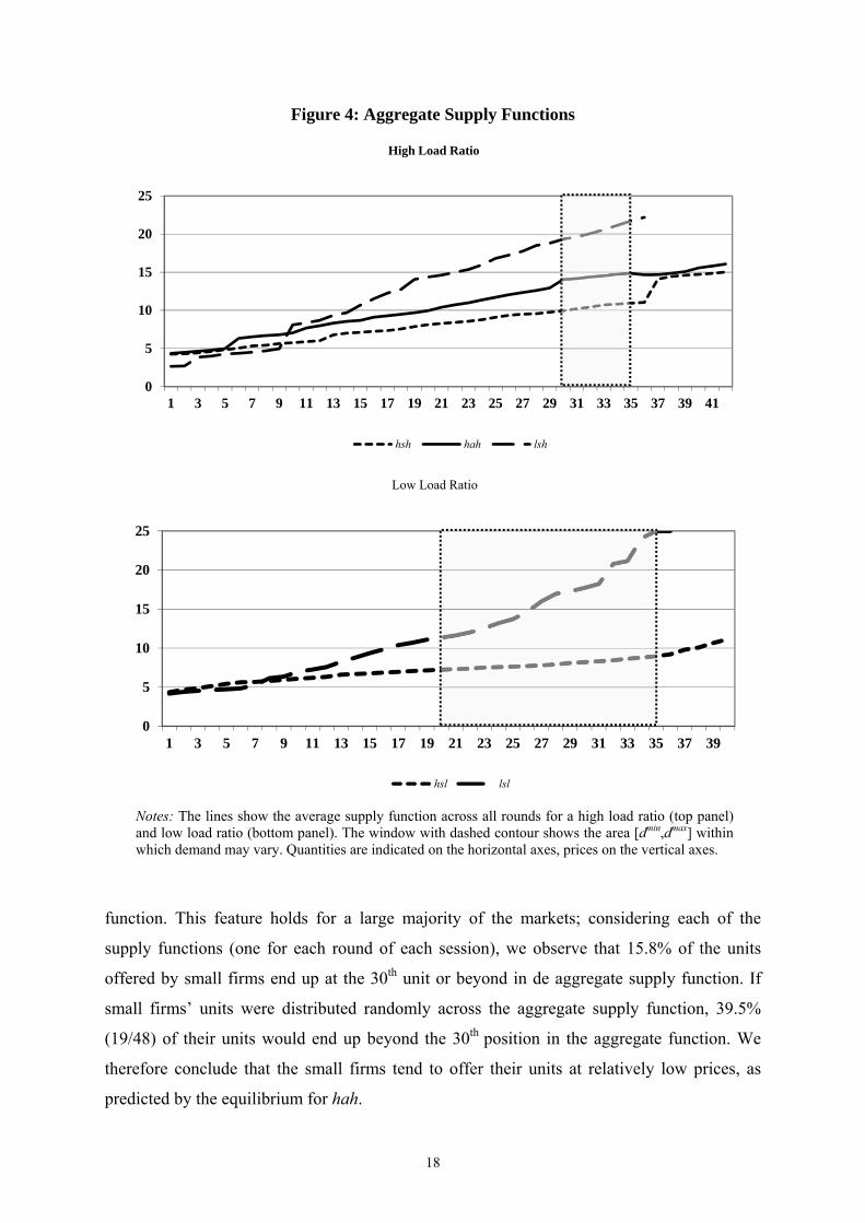
Figure 4: Aggregate Supply Functions

Notes: The lines show the average supply function across all rounds for a high load ratio (top panel) and low load ratio (bottom panel). The window with dashed contour shows the area [dmin,dmax] within which demand may vary. Quantities are indicated on the horizontal axes, prices on the vertical axes.

function. This feature holds for a large majority of the markets; considering each of the

supply functions (one for each round of each session), we observe that 15.8% of the units

offered by small firms end up at the 30th unit or beyond in de aggregate supply function. If

small firms’ units were distributed randomly across the aggregate supply function, 39.5%

(19/48) of their units would end up beyond the 30th position in the aggregate function. We

therefore conclude that the small firms tend to offer their units at relatively low prices, as

predicted by the equilibrium for hah.

0

5

10

15

20

25

1 3 5 7 9 11 13 15 17 19 21 23 25 27 29 31 33 35 37 39 41

High Load Ratio

hsh hah lsh

0

5

10

15

20

25

1 3 5 7 9 11 13 15 17 19 21 23 25 27 29 31 33 35 37 39

Low Load Ratio

hsl lsl

19

Figure 5: Aggregate Supply Functions Small and Large Firms

Notes: The lines show the average supply function across all rounds for small (short line) and large (long line) firms. Quantities are indicated on the horizontal axes, prices on the vertical axes.

Table 4 shows volume weighted average prices both for all rounds and for the last 5 rounds,

averaged over all groups of each treatment, together with the equilibrium predictions for the

two models we consider.

Table 4: Predicted and Actual Volume Weighted Average Prices

Equilibrium Predictions Actual

MUA SFE SFE:

midpoint

SFE: payoff

dominant

All rounds

Last 5 rounds

High Load Ratio High Sym Cap(hsh) [5,7.5] [5, 21.3] 13.2 21.3 10.53 9.30 Low Sym Cap (lsh) > 18.5 [18,21.3]&{25} 19.7 25 20.48 20.02 High Asym Cap (hah)

{25} [11.2,23.1]&{25} 17.2 25 14.47 13.47

Low Load Ratio High Sym Cap (hsl) [5,5.75] [5, 16.4] 10.7 16.4 8.07 7.00 Low Sym Cap (lsl) > 11.6 [12.4, 16.4] 14.4 16.4 16.56 18.02

We calculated the realized VWAP by a group in a round by using the aggregate submitted

supply function and determining the expected VWAP across the possible demand

realizations.21 In cases where fewer units are offered at a price lower than the maximum than

are demanded for some realizations, total supply is offered at the maximum price and we use

the quantity traded to determine the weights.22

21 Alternatively, one could use the realized demand in the five periods of the round. The outcome then depends on the realized draws of demand, however. Because we aim at testing hypotheses derived from strategies used and because the information about the strategies is contained in the aggregate supply function, we prefer to use the expected demand to weight the supply prices with. 22For example, assume for a high-load case that only 34 units are offered. Units 30, 31…, 34 are offered at prices 10,11…, 14, respectively. For demand realization d<35, these are also the (uniform) trading prices and all units are sold. If d=35, then

0

5

10

15

20

25

1 4 7 10 13 16 19 22 25 28 31 34 37

20

Focus first on the two cases with high symmetric capacity, hsh and hsl. For both load

ratios prices are within the range of the SFE predictions, but below the two refinements and

above the prediction of the MUA. Note also that prices are lower in the last five rounds than

in earlier rounds. This means that they are moving away from the SFE refinements and in the

direction of the MUA predictions. For low symmetric capacity with the high load ratio, lsh,

prices are again within the interval of the SFE. They are close to the SFE midpoint

refinement and below the SFE payoff dominant. They are also above the lower limit of the

mixed strategy equilibrium support for the MUA. For lsl, observe that prices are somewhat

above the upper limit of the SFE interval and therefore above both refinements. They are also

above the lower limit of the mixed-strategy equilibrium support. Finally, for the high

asymmetric case, hah, prices are within the SFE interval and below all point predictions.23

Formal tests of differences in average VWAP are presented below, when we discuss the

results for our hypotheses testing.

Given that average prices are (slightly) different in the final five rounds than across all

rounds, the dynamics of the VWAP may be important. Therefore, we now examine how these

prices changed across rounds. Figure 6 presents their development across rounds, separately

for each treatment. Starting with the symmetric treatments, figure 6 shows that prices for both

low capacity treatments lsl and lsh are substantially and consistently above those for the high

capacity treatments hsl and hsh. The differences increase over rounds: the primary reason is

that average prices for high symmetric capacity treatments decrease steadily. This decrease

across rounds is statistically significant. Linearly regressing the VWAP on the round gives

coefficient –0.13 for hsl and –0.14 for hsh, both with p-values <0.001.

Comparing hsh to hsl one can see that prices for the former are above those for hsl in all

rounds. In addition, average prices in these high symmetric capacity experiments are above

the (highest) MUA predictions of 7.5 (hsh) and 5.75 (hsl) in all rounds. Thus, aggregate

behavior in these high symmetric capacity experiments appears to be inconsistent with MUA

predictions, although prices are slowly moving toward the MUA prediction over time. We

will explore this issue further when we examine data from individual markets. The ordering

of average prices in hsh and hsl would be consistent with a single upward sloping aggregate

34 units are sold at p=25. The average quantity traded is then 1/6*(30+31+…+34+34)=32.33. The VWAP is 1/6*{(30/32.33)*10+(31/32.33)*11+…+(34/32.33)*14+(34/32.33)*25}=14.33. 23 The fact that prices stay away from the extreme predictions of the MUA could be attributed to a behavioral tendency not to choose prices at the edges of the choice space. However, it is worth pointing out here that in experiments with the double auction and the box demand design prices often do go all the way to the extremes (Davis and Holt, 1993).

21

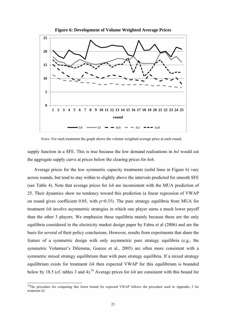
Figure 6: Development of Volume Weighted Average Prices

Notes. For each treatment the graph shows the volume weighted average price at each round.

supply function in a SFE. This is true because the low demand realizations in hsl would cut

the aggregate supply curve at prices below the clearing prices for hsh.

Average prices for the low symmetric capacity treatments (solid lines in Figure 6) vary

across rounds, but tend to stay within to slightly above the intervals predicted for smooth SFE

(see Table 4). Note that average prices for lsh are inconsistent with the MUA prediction of

25. Their dynamics show no tendency toward this prediction (a linear regression of VWAP

on round gives coefficient 0.05, with p=0.35). The pure strategy equilibria from MUA for

treatment lsh involve asymmetric strategies in which one player earns a much lower payoff

than the other 3 players. We emphasize these equilibria mainly because these are the only

equilibria considered in the electricity market design paper by Fabra et al (2006) and are the

basis for several of their policy conclusions. However, results from experiments that share the

feature of a symmetric design with only asymmetric pure strategy equilibria (e.g., the

symmetric Volunteer’s Dilemma, Goeree et al., 2005) are often more consistent with a

symmetric mixed strategy equilibrium than with pure strategy equilibria. If a mixed strategy

equilibrium exists for treatment lsh then expected VWAP for this equilibrium is bounded

below by 18.5 (cf. tables 3 and 4).24 Average prices for lsh are consistent with this bound for

24The procedure for computing this lower bound for expected VWAP follows the procedure used in Appendix 2 for treatment lsl.

0

5

10

15

20

25

1 2 3 4 5 6 7 8 9 10 11 12 13 14 15 16 17 18 19 20 21 22 23 24 25

round

lsh lsl hsh hsl hah

22

expected VWAP. Average prices for lsl are consistent with the MUA prediction, in the sense

that they are also above the lower bound prediction for the mixed strategy MUA equilibrium.

There is a marginally significant upward trend (coefficient 0.06, with p=0.08).

Finally, average prices for hah vary over rounds but tend to lie within the interval of

equilibrium prices for smooth SFE. In later rounds, average prices are in the lower portion of

this predicted interval. The decreasing trend is marginally significant (coefficient –0.09,

p=0.06) Average prices for hah are clearly inconsistent with the pure strategy equilibrium

prediction of 25 for MUA. If anything, they are converging away from this predicted level.

We conclude that the time trends in our data could be interpreted as convergence in the

direction of the MUA prediction only in the symmetric high capacity cases. As for the two

SFE refinements, a comparison between figure 6 and the predictions in table 3 reveals that

the data do not appear to be converging towards either prediction in any of the treatments.

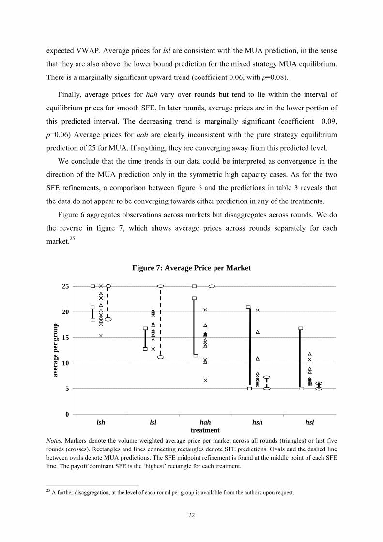
Figure 6 aggregates observations across markets but disaggregates across rounds. We do

the reverse in figure 7, which shows average prices across rounds separately for each

market.25

Figure 7: Average Price per Market

Notes. Markers denote the volume weighted average price per market across all rounds (triangles) or last five rounds (crosses). Rectangles and lines connecting rectangles denote SFE predictions. Ovals and the dashed line between ovals denote MUA predictions. The SFE midpoint refinement is found at the middle point of each SFE line. The payoff dominant SFE is the ‘highest’ rectangle for each treatment.

25 A further disaggregation, at the level of each round per group is available from the authors upon request.

0

5

10

15

20

25

lsh lsl hah hsh hsl

aver

age

per

gro

up

treatment

23

To highlight the effects of learning we distinguish between the average across all rounds and

the average across the final five rounds. This figure confirms that just like the aggregate

prices (figure 6), the average prices per market lie largely within the bounds predicted by

SFE. In the absence of market power, the observations for hsh and hsl appear to be drawn

towards the competitive prices predicted by MUA. For each of these two treatments, all

groups but one had average prices at the MUA prediction for the last five rounds. For the

treatments with market power, the observations appear to be more or less uniformly spread

over the predicted interval of smooth SFE prices.26

Our symmetric, high-capacity treatments (hsh and hsl) are similar in some respects to the

multi-unit sales auction experiments reported on in Sefton and Zhang (2010). In their no-

communication treatment, they find that subjects’ bids converge to their values, which is

consistent with pure strategy Nash equilibrium.27 By contrast, some offers remained above

the discrete-units Nash prediction of offers equal to marginal cost for some groups in our hsh

and hsl treatments. Factors that might account for the differences in results include relatively

greater excess capacity in Sefton and Zhang and a random demand quantity in our

experiments compared to the fixed sales quantity in Sefton and Zhang.

We now move to the tests of the hypotheses 1 to 6 about differences in prices across

treatments presented in section 3.28 Table 5 presents the results of Mann-Whitney tests for all

pairwise differences in means across the five treatments. It takes the (volume weighted)

average price per market (across all rounds) as the unit of observation. The p-values

pertaining to our six hypotheses are shown in italics. For the hypotheses, we only need to

consider these results. Observe that five out of six of the differences in italics are statistically

Table 5: Pairwise Mann-Whitney Tests for Volume Weighted Average Prices

hsl hah lsh lsl hsh 0.165 0.089 0.004 0.009 hsl - 0.002 0.002 0.001 hah - - 0.002 0.047 lsh - - - 0.002

Notes. Cell entries give the p-value for the Mann-Whitney test for the null hypothesis that the dif-ference in means between the treatments in the row and column concerned are equal to zero. Group averages across rounds are taken as the units of observation.Results in italics are relevant for the hypotheses developed in section 3, as explained in the main text.

26 Note that for lsh there is one group that has VWAP at the pure strategy MUA prediction of 25 in the last 5 rounds. In the MUA equilibrium, three firms offer all units at a low price and one firm offers all units at a price of 25. The data for this group reveal that there are two firms offering all units at a low price and two firms offering at the price cap. 27As noted in fn. 11, there are multiple pure strategy equilibria in the Sefton and Zhang design, including some with collusive bidding. 28 Given the directional nature of our hypotheses, the p-values reported in Table 5 are based on one-tailed tests. All other p-values in this section are based on two-tailed tests.

24

significant at the 10%-level or better (four are significant at the 1%-level) and therefore

support the alternative hypotheses against the null of no differences in average prices.

We summarize the results of our hypotheses testing in the following way:

(1) for H1-H3, the alternative hypotheses are supported: symmetrically decreasing

capacity (with either load ratio) and asymmetrically redistributing a given total capacity (with

the high load ratio) all have the positive effects on prices predicted by the RSI and both

theoretical models. In other words, when the RSI, MUA and at least one SFE refinement all

yield the same comparative static prediction, this is confirmed by our data.

(2) for H4, the alternative hypothesis is supported: with a high load ratio, market power

caused by a symmetric reduction in capacity has a stronger effect than market power caused

by asymmetry; this is in accordance with the hypothesis based on the RSI and the SFE

midpoint refinement, while MUA and the payoff-dominant SFE are mute on this particular

comparison.

(3) for H5, the null hypothesis cannot be rejected: with high symmetric capacity the

change from a low to a high load ratio does not significantly affect prices, an effect predicted

both by RSI and the two SFE refinements. Note that the VWAP for a low load ratio the

possible demand realizations include the demand set for a high load ratio. In addition, lower

levels of demand (i.e, between 20 and 29) are possible. With a non-decreasing aggregate

supply function this may load the deck in favor of a higher VWAP when the load ratio is

high. Though a formal test of H4 requires comparison across the two demand domains, for

completeness’ sake we also present the comparison for the case where demand is restricted to

{30,…,35}. We then find that the average VWAP is still higher with a high load ratio (10.53

versus 8.59), but the difference is not statistically significant (Mann Whitney, N=11,

p=0.165).29

(4) for H6, the alternative hypothesis is supported: for low symmetric capacity, the

change in load ratio does lead to higher prices, an effect predicted by RSI, MUA and both

SFE refinements. We again present the comparison for the case where demand is restricted to

{30,…,35}. The average VWAP is again higher with a high load ratio (20.48 versus 19.57),

but the difference is not statistically significant (Mann Whitney, N=11, p=0.396).

29We thank an anonymous referee for suggesting this additional test.

25

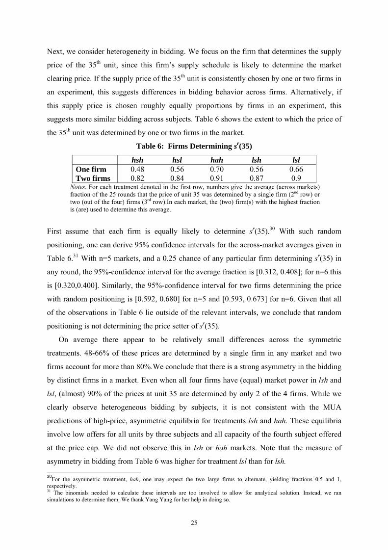
Next, we consider heterogeneity in bidding. We focus on the firm that determines the supply

price of the 35th unit, since this firm’s supply schedule is likely to determine the market

clearing price. If the supply price of the 35th unit is consistently chosen by one or two firms in

an experiment, this suggests differences in bidding behavior across firms. Alternatively, if

this supply price is chosen roughly equally proportions by firms in an experiment, this

suggests more similar bidding across subjects. Table 6 shows the extent to which the price of

the 35th unit was determined by one or two firms in the market.

Table 6: Firms Determining sr(35)

hsh hsl hah lsh lsl One firm 0.48 0.56 0.70 0.56 0.66 Two firms 0.82 0.84 0.91 0.87 0.9

Notes. For each treatment denoted in the first row, numbers give the average (across markets) fraction of the 25 rounds that the price of unit 35 was determined by a single firm (2nd row) or two (out of the four) firms (3rd row).In each market, the (two) firm(s) with the highest fraction is (are) used to determine this average.

First assume that each firm is equally likely to determine sr(35).30 With such random

positioning, one can derive 95% confidence intervals for the across-market averages given in

Table 6.31 With n=5 markets, and a 0.25 chance of any particular firm determining sr(35) in

any round, the 95%-confidence interval for the average fraction is [0.312, 0.408]; for n=6 this

is [0.320,0.400]. Similarly, the 95%-confidence interval for two firms determining the price

with random positioning is [0.592, 0.680] for n=5 and [0.593, 0.673] for n=6. Given that all

of the observations in Table 6 lie outside of the relevant intervals, we conclude that random

positioning is not determining the price setter of sr(35).

On average there appear to be relatively small differences across the symmetric

treatments. 48-66% of these prices are determined by a single firm in any market and two

firms account for more than 80%.We conclude that there is a strong asymmetry in the bidding

by distinct firms in a market. Even when all four firms have (equal) market power in lsh and

lsl, (almost) 90% of the prices at unit 35 are determined by only 2 of the 4 firms. While we

clearly observe heterogeneous bidding by subjects, it is not consistent with the MUA

predictions of high-price, asymmetric equilibria for treatments lsh and hah. These equilibria

involve low offers for all units by three subjects and all capacity of the fourth subject offered

at the price cap. We did not observe this in lsh or hah markets. Note that the measure of

asymmetry in bidding from Table 6 was higher for treatment lsl than for lsh. 30For the asymmetric treatment, hah, one may expect the two large firms to alternate, yielding fractions 0.5 and 1, respectively. 31 The binomials needed to calculate these intervals are too involved to allow for analytical solution. Instead, we ran simulations to determine them. We thank Yang Yang for her help in doing so.

26

Now we take a closer look at the degree of rationality of the behavior we observe. Since

we have detailed data on round-by-round offers submitted by subjects it is possible for us to

assess the extent to which individual choices are best responses to choices made by rival

subjects.32 We would not expect outcomes in the experiment to be consistent with Nash

equilibrium predictions unless subjects are making best responses to rivals’ choices. The

game that subjects are playing is complex with a very large strategy set. Both MUA and SFE

predict multiple equilibria. In addition, our subjects have only limited feedback regarding

auction results. After each period (there are 5 periods per round) subjects observe the market

clearing price, the quantity demanded, and the position of their own offers in the aggregate

offer queue; see Figure 1. Subjects do not directly observe the offers made by other subjects,

although they may be able to infer approximate offers of rivals. Given the size of the strategy

set, multiplicity of equilibria, and limited information feedback, it is not at all obvious that

subjects would play best responses in the experiments.

In order to assess individual choices we compare the actual profit of subjects to what we

call ex-post optimal profit.33 We calculate the ex-post optimal profit for a subject in a round

of play by finding an offer that yields the highest possible profit given the actual offers

submitted by other subjects for that round.34 Note that a subject’s ex-post optimal offer in a

particular round need not be unique. For example, if rival subjects submit relatively high

offers then a subject’s best response would be any offer schedule that offers all units up to

capacity at prices below rivals’ offers, allowing the market price to be dictated by rivals’

offers.35

Table 7 summarizes results for actual profit as a percentage of ex-post optimal profit over

all rounds for each subject. This figure ranged between 100%and 29%, with a median of 79%

across all 112 subjects in the experiments. There are differences in actual/ex post optimal

profit across decision-making conditions. Differences across all symmetric treatments are

statistically significant (KW, 2=15.10, p=0.00, N=22), as are differences between high- and

low-capacity subjects in the asymmetric treatment (MW, Z=2.21, p=0.03, N=6 paired

32 Note that we consider here the round-by-round best response and neglect the possibility of strategic play across rounds (which would be very difficult to implement). Moreover, ex post (i.e., after realization of demand), the optimal profit based on a best response may not be attainable. 33A similar approach of comparing actual profit to ex-post optimal profit was used in Hortacsu and Puller (2008) in their examination of behavior of electricity generation suppliers in the Texas ERCOT wholesale power balancing market. We compare the results of our analysis to theirs, below. 34 The set of possible offer schedules for high-capacity subjects in hah is extremely large. For these subjects we approximate the best response in each round by sampling from the set of possible offers. 35 Similarly, for actual profit, we do not take the realized profit after demand realization, but the expected profit, given the subject's own supply curve, its rivals' actual aggregate supply curve, and the distribution of demand quantities. This ensures that actual profits cannot exceed ex-post optimal profits. We thank an anonymous referee for suggesting this procedure.

27

Table 7: Actual Subject Profit as Percent of Ex-post Optimal Profit

#units Median Max Min

high load ratio

symmetric high capacity (hsh) 12 66 (€14.05) 79 42 low capacity (lsh) 9 84 (€12.79) 100 73

asymmetric (hah-high capacity trader) 19 80 (€14.42) 96 61 (hah-low capacity trader) 5 88 (€2.89) 100 61

low load ratio

symmetric high capacity (hsl) 12 45 (€19.42) 66 29 low capacity (lsl) 9 85 (€7.97) 99 66

All subjects -- 79 100 29 Notes. Numbers represent average/ex post optimal profit for the treatment concerned. Ex post optimal profits were calculated in the way described in the main text. The column #units gives the maximum number of units each trader had available to offer. To see why a ratio larger than 100 may occur, see footnote 23. The amount in parentheses in euro’s denotes the median loss in euro’s that follows from the median suboptimal choice.

observations). Subjects with a small amount of capacity (low capacity subjects in hah and

subjects in treatments lsh and lsl) have higher average actual/ex post optimal profit than sub

jects with higher capacity (high capacity subjects in hah and subjects in treatments hsl and

hsh). More specifically, from high to low, the treatment-average actual/ex post optimal profit

is ordered as follows:

hahlow>0.662lsh>0.792lsl>0.030hahhigh>0.004hsh>0.004hsl

where hahlow (hahhigh) refers to the low (high) capacity traders in hah and >xx indicates the p-

value of the Mann-Whitney test of the difference concerned (using market averages as units

of observations). These tests confirm that the percentage of actual to ex post optimal profit is

significantly greater the lower the capacity per subject. It appears that the larger strategy sets

associated with greater capacity contribute to a more complex decision making environment

and greater departures from optimality.36 Finally, note that the numbers in euro’s show that

the losses due to suboptimal responses are substantial.

Hortacsu and Puller (2008) conduct a similar analysis using market data and report on

actual profit vs. ex post optimal profit for firms that offer electricity generation into the

ERCOT wholesale power balancing market. It is possible to make these calculations because

of the detailed information available about generation costs and about bids submitted by

firms. They use data from a single trading period within each day (6 – 6:15 pm) for days that

did not experience transmission congestion across zones within ERCOT. The reported results

for actual to ex post optimal profit range from a high of 79% to a low of 81 %; the median

figure for the sample of 35 firms is 15%. This contrasts with results from our experiments; 36 Note, however, that the percentage is significantly higher in the 19-unit hahhigh case than in the 12 unit hsh and hsl cases. This may be due to the fact that subjects in hahhigh have to deal with only one other large firm.

28

approximately half of our subjects achieved higher actual to ex post optimal profit than the

firm with the highest percentage in the Hortacsu and Puller study.

Hortascsu and Puller (2008) also found differences in performance across firms, but

seemingly in the opposite direction of our experimental results. They find that large firms

(those with a high volume of sales under ex post optimal bidding) have significantly higher

actual/ex post optimal profit than smaller firms. Hortacsu and Puller attribute this result to the

fixed costs associated with activities required in order to profit in the balancing market:

acquiring information, analyzing information, and running a trading operation. The higher

profit stakes available to larger firms made it worthwhile for them to invest in the fixed costs,

but the lower profit stakes for small firms left them with weak incentives to invest. By

contrast, subjects in our experiments did not bear any costs of participating in the market

except perhaps the opportunity cost of their attention.

This difference in results from the field and the laboratory are interesting.37 They point to

the particular advantages both methods have. On the one hand, the advantage of laboratory

control is that it allows us to isolate causal effects when comparing realized-profit-to-optimal-

profit ratios across distinct environments. They are less informative about the actual level of

such ratios, however. For this, data from the field are more relevant. Moreover, our

laboratory data allow us to isolate the effects of production capacity holding other

characteristics (such as fixed costs) constant, while the field data allow for a comparison

between large en small firms that take into account all differences between the two.

As a final exercise, we turn to an assessment of the theoretical predictions of market

prices. The SFE and MUA models each provide equilibrium predictions of prices. We do not

attempt to compare directly the predictive success of the MUA model to the complete set of

equilibria predicted by the SFE model because the latter model predicts large intervals of

equilibrium prices for every treatment and MUA equilibrium prices are a small subset of SFE

prices. What we do instead is to simply report on test statistics for predictive success for

MUA, for unrestricted SFE and for the two refinements of SFE distinguished above.

The following statistical model is the basis for the tests. Let,

pij= average VWAP for group i of treatment j, j {lsl, lsh, hsl, hsh, hah}

37 Our laboratory market experiments differ from the ERCOT energy balancing market in several ways. Subjects in our experiments make repeated decisions in markets with stable costs and capacities, and a fixed group of participants. The ERCOT market environment is considerably more complex. It involves costs and capacities that change from day to day (e.g., due to generation outages, fuel cost changes and contractual commitments), several different types of generation, start-up and ramping costs for generation, and changes in the set of market participants over time. Given these differences between our experiments and the ERCOT environment, we would not necessarily expect to see similar ratios of actual to optimal profit.

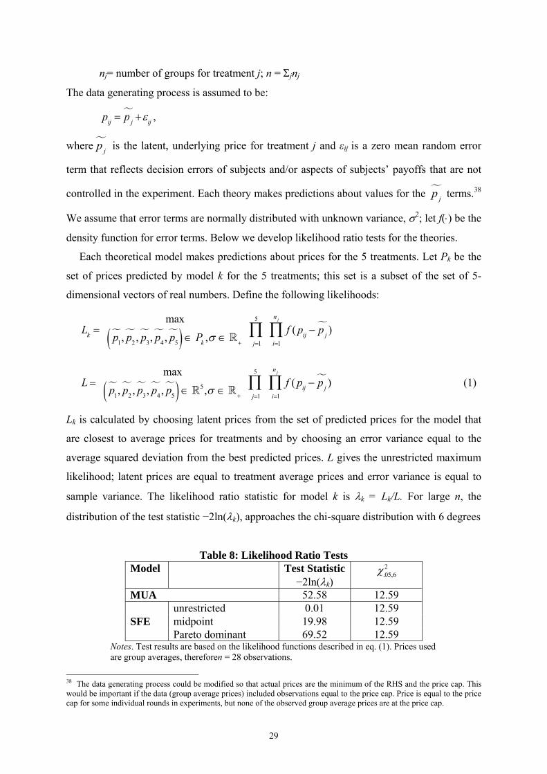
29

nj= number of groups for treatment j; n = jnj

The data generating process is assumed to be:

pij p

j

ij,

where pj

is the latent, underlying price for treatment j and εij is a zero mean random error

term that reflects decision errors of subjects and/or aspects of subjects’ payoffs that are not

controlled in the experiment. Each theory makes predictions about values for the pj

terms.38

We assume that error terms are normally distributed with unknown variance, 2; let f() be the

density function for error terms. Below we develop likelihood ratio tests for the theories.

Each theoretical model makes predictions about prices for the 5 treatments. Let Pk be the

set of prices predicted by model k for the 5 treatments; this set is a subset of the set of 5-

dimensional vectors of real numbers. Define the following likelihoods:

Lk

max

p1 , p

2 , p

3 , p

4 , p

5 P

k, j1

5

f ( pij p

j

i1

n j

)

L max

p1 , p

2 , p

3 , p

4 , p

5 5, j1

5

f ( pij p

j

i1

n j

) (1)

Lk is calculated by choosing latent prices from the set of predicted prices for the model that

are closest to average prices for treatments and by choosing an error variance equal to the

average squared deviation from the best predicted prices. L gives the unrestricted maximum

likelihood; latent prices are equal to treatment average prices and error variance is equal to

sample variance. The likelihood ratio statistic for model k is k = Lk/L. For large n, the

distribution of the test statistic −2ln(k), approaches the chi-square distribution with 6 degrees

Table 8: Likelihood Ratio Tests Model Test Statistic

−2ln(k)

2.05,6

MUA 52.58 12.59

SFE unrestricted 0.01 12.59

midpoint 19.98 12.59

Pareto dominant 69.52 12.59 Notes. Test results are based on the likelihood functions described in eq. (1). Prices used are group averages, thereforen = 28 observations.

38 The data generating process could be modified so that actual prices are the minimum of the RHS and the price cap. This would be important if the data (group average prices) included observations equal to the price cap. Price is equal to the price cap for some individual rounds in experiments, but none of the observed group average prices are at the price cap.

30

of freedom. Table 8 reports results for tests of the hypothesis that latent prices for treatments

are in the set of equilibrium prices predicted by theoretical models. We use a 95 percent

confidence interval for the tests. Values of the test statistic that are larger than 2.05,6 therefore

reject the null hypothesis that our data are generated by the model concerned.

We observe that the only model that is not rejected by the test is the unrestricted SFE

model, for which we calculate SFE=0.993, yielding a test statistic close to zero. This result

reflects that there are SFE equilibrium price predictions that are either equal to or close to

average observed prices for each treatment. For the restricted SFE models and the MUA

model we find that the test statistics exceed the 2 statistic and therefore reject the hypothesis

that observed group average prices are drawn from distributions with mean values in the

equilibrium sets for these models.39 As mentioned above, this higher predictive power if the

unrestricted SFE model comes at a cost, however. The unrestricted SFE model is far less

parsimonious than either of its refinements or the MUA alternative. The bottom line remains,

however, that we have found no more parsimonious model capable of organizing our data in

a satisfactory way.

5. Concluding Discussion

We set out to experimentally study the effects of pivotal power, motivated both by the results

of empirical field data studies and by the predictions of recent theoretical models. A first

conclusion from our experiments is that the more fundamental intuitions about the impact of

pivotal power are supported by our data. Prices are higher when (some) firms are pivotal. The

existence of aggregate excess capacity is not enough to guarantee competitive prices. This

general result is accordance both with the predictions of the intuitive RSI and of the SFE

model based on divisible output and MUA modelbased on discrete output units.

Our experiments also permit us to assess in more detail the predictive power of these

theoretical models as well as of two refinements of the SFE model. The MUA model

provides sharp predictions for 3 out of our 5 treatments; for these treatments pure strategy

equilibria of the MUA predict either near competitive pricing or monopoly pricing. The SFE

model predicts a larger set of equilibria that includes the sharp MUA equilibria as well as

additional equilibria based on upward sloping supply functions. One can see the SFE model

prescriptions as a more modest proposal for organizing observed behavior, in contrast to the 39The likelihood for MUA is computed using the lower bound for VWAP from a mixed strategy equilibrium condition for treatment lsh. If we restrict MUA predictions to those from pure strategy equilibria for lsh then the test statistic is higher and MUA is rejected more decisively.

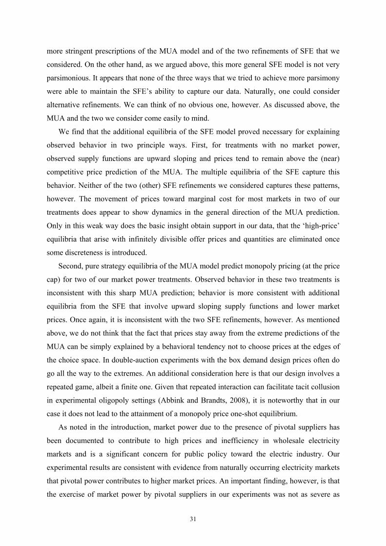
31

more stringent prescriptions of the MUA model and of the two refinements of SFE that we

considered. On the other hand, as we argued above, this more general SFE model is not very

parsimonious. It appears that none of the three ways that we tried to achieve more parsimony

were able to maintain the SFE’s ability to capture our data. Naturally, one could consider

alternative refinements. We can think of no obvious one, however. As discussed above, the

MUA and the two we consider come easily to mind.

We find that the additional equilibria of the SFE model proved necessary for explaining

observed behavior in two principle ways. First, for treatments with no market power,

observed supply functions are upward sloping and prices tend to remain above the (near)

competitive price prediction of the MUA. The multiple equilibria of the SFE capture this

behavior. Neither of the two (other) SFE refinements we considered captures these patterns,

however. The movement of prices toward marginal cost for most markets in two of our

treatments does appear to show dynamics in the general direction of the MUA prediction.

Only in this weak way does the basic insight obtain support in our data, that the ‘high-price’

equilibria that arise with infinitely divisible offer prices and quantities are eliminated once

some discreteness is introduced.

Second, pure strategy equilibria of the MUA model predict monopoly pricing (at the price

cap) for two of our market power treatments. Observed behavior in these two treatments is

inconsistent with this sharp MUA prediction; behavior is more consistent with additional

equilibria from the SFE that involve upward sloping supply functions and lower market

prices. Once again, it is inconsistent with the two SFE refinements, however. As mentioned

above, we do not think that the fact that prices stay away from the extreme predictions of the

MUA can be simply explained by a behavioral tendency not to choose prices at the edges of

the choice space. In double-auction experiments with the box demand design prices often do

go all the way to the extremes. An additional consideration here is that our design involves a

repeated game, albeit a finite one. Given that repeated interaction can facilitate tacit collusion

in experimental oligopoly settings (Abbink and Brandts, 2008), it is noteworthy that in our

case it does not lead to the attainment of a monopoly price one-shot equilibrium.

As noted in the introduction, market power due to the presence of pivotal suppliers has

been documented to contribute to high prices and inefficiency in wholesale electricity

markets and is a significant concern for public policy toward the electric industry. Our

experimental results are consistent with evidence from naturally occurring electricity markets

that pivotal power contributes to higher market prices. An important finding, however, is that

the exercise of market power by pivotal suppliers in our experiments was not as severe as

32

equilibrium predictions of the MUA model. These predictions require that agents adopt

strategies that support an asymmetric equilibrium with payoffs that differ substantially across

agents (even for agents with identical costs and capacities). Experimental results for

treatments with pivotal suppliers were more consistent with SFE predictions involving lower

prices.

A final result that we wish to highlight here pertains to the effects of increasing the load

ratios. We find that when both models suggest that it will affect prices it does have this effect.

We interpret this as indicating that the models do identify a potential influence factor, but that

it only shows up in the data when it is a strong force. Stronger variations in demand reduce

market power, in a situation where this power is otherwise strongest.

33

Appendix 1

This appendix gives the English translation of the original Dutch instructions for the sessions with symmetric high capacity (12 units per producer) and low load ratio. The instructions were programmed as html pages. Horizontal lines indicate page separations. INSTRUCTIONS You are about to participate in an economic experiment. The instructions are simple. if you follow them carefully, you can make a substantial amount of money. Your earnings will be paid to you in euro’s at the end of the experiment. In the experiment, we use the currency 'franc'. At the end of the experiment, we will exchange the francs for guilders. The exchange rate to be used is 1 euro for 250 francs. For each 1000 francs, you will therefore receive € 4. We will use numerical examples in these instructions. These are only meant to be an illustration and are irrelevant for the experiment itself. In these instructions, you may click on the links at the bottom of each page to move forward or backward. Sometimes, there will be more text on a page than can fit onto your screen. When that is the case, you can use the scroll bar on the right to move down. Next page ROUNDS AND PERIODS The experiment will consist of 25 rounds today, preceded by5 practice rounds. In the 25 rounds, you will be a member of a group. Aside from you, the group will consist of 3 other people. The composition of the group is anonymous. You will not know who is in the group with you. Others will not know that you are in their group. The composition of your group is the same for the whole experiment. You will have nothing to do with people in other groups. In the experiment, you will participate in a market, in which fictitious goods will be produced and sold. The final consumers of the good will be simulated by the computer. All participants will be producers of the good. There are 4 producers in each group. In the practice rounds, you will not be in a group with other participants. The computer will simulate the choices of other group members. It does so in a completely random manner. You cannot learn anything about others' behavior from these simulated choices. Each round will consist of 5 periods. In each period, the computer will decide how many of the goods to buy. You do not need to do anything between periods. At the beginning of the round, you will decide how many units you are willing to produce and sell.

34

This choice will be valid in each of the 5 periods in that round. The remainder of these instructions will explain the market and the rules you must abide by. previous page next page SIMULATED BUYERS In this experiment, the decisions to buy (fictitious) goods are not made by participants but by the computer. This will be done as follows. In each period, the computer will buy between 20 and 35 units of the good. Each number between 20 and 35 (inclusive) is equally likely. Because there are 16 integer numbers between 20 and 35, in each period there is a probability of 1/16 that any one of these number will be drawn. After a number has been drawn, it may be drawn again in a next period of a round. To determine the price that the computer will pay per unit bought in a period, it is determined at what (minimum) prices the group members are willing to sell each unit. Below, we will explain how this determines the price paid by the computer. The computer will never pay more than 25 francs per unit, however. If not enough sellers are willing to sell for a price lower than 25, the computer will buy as many as it can for 25 francs. previous page next page PRODUCTION AND COSTS At the beginning of the experiment, each participant will receive 1250 francs as a starting capital. You will see this amount on your screen when the experiment starts. In each round, each participant is a producer who must decide how many units of the good he or she wishes to produce. No producer is allowed to produce more than 12 units. For each unit a producer is willing to produce, he or she must determine the minimum price that he or she wishes to receive for that unit. We will call this the 'ask price'. How this is reported, will be explained shortly. There are costs related to producing goods. For each unit you produce, you must pay 5 francs. previous page next page ASK PRICES

35

For each unit you would like to offer, you need to indicate at what price (the 'ask price') you are willing to sell it. You may ask different prices for distinct units. For this, the following rules apply. If you offer a unit for sale, you must also offer all preceding units. For example, if you indicate a minimum price asked for unit 3, you must also offer units 1 and 2. Your price asked for a unit must always be higher than or equal to the price asked for the preceding unit. So: your ask price for the second unit may not be lower than for the first unit. Your ask price for the third unit may again not be lower than your ask price for the second unit, etc. Each producer can produce at most 12 units. Your ask price may be lower than the costs. Note that you may make a loss on that unit in that case. For example.assume that your price asked for the first three units is 3. Assume that the three units are bought by the computer at a price of 4. For each unit, your production costs are 5 and your revenue is 4, so you make a loss of 1. For the three units together, your loss is 3. All units for which you ask a positive price are offered on the market. However, a unit is only sold if the computer is willing to pay your ask price for that unit. How this is determined will be discussed shortly. previous page next page SUBMITTING YOUR ASK PRICES

To enter your ask prices, you will use a window that looks like this. Note that you can only see the first 4 units. In the experiment, you will be able to scroll down to the other units. This is not possible in these instructions. The first column (nr) indicates the number of the unit. The second column (cost) gives the cost per unit (5). The next column (cumm) gives the total costs for that level of production. The last column (ask price) will be used to enter the minimum price you wish to receive for that unit. You indicate your willingness to sell units by entering the amount you want to receive in the column ask price. It is up to you to decide how many different numbers you wish to enter, as long as no ask price is lower than the preceding one. You may enter a different number for

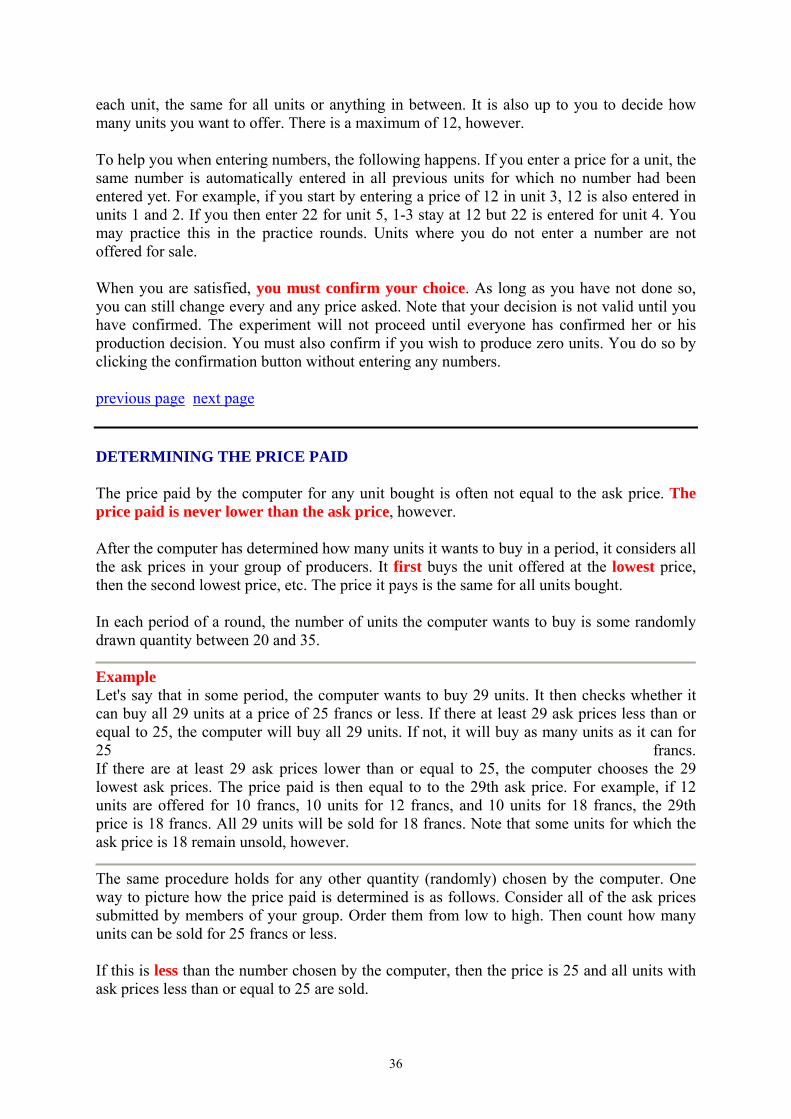
36

each unit, the same for all units or anything in between. It is also up to you to decide how many units you want to offer. There is a maximum of 12, however. To help you when entering numbers, the following happens. If you enter a price for a unit, the same number is automatically entered in all previous units for which no number had been entered yet. For example, if you start by entering a price of 12 in unit 3, 12 is also entered in units 1 and 2. If you then enter 22 for unit 5, 1-3 stay at 12 but 22 is entered for unit 4. You may practice this in the practice rounds. Units where you do not enter a number are not offered for sale. When you are satisfied, you must confirm your choice. As long as you have not done so, you can still change every and any price asked. Note that your decision is not valid until you have confirmed. The experiment will not proceed until everyone has confirmed her or his production decision. You must also confirm if you wish to produce zero units. You do so by clicking the confirmation button without entering any numbers. previous page next page DETERMINING THE PRICE PAID The price paid by the computer for any unit bought is often not equal to the ask price. The price paid is never lower than the ask price, however. After the computer has determined how many units it wants to buy in a period, it considers all the ask prices in your group of producers. It first buys the unit offered at the lowest price, then the second lowest price, etc. The price it pays is the same for all units bought. In each period of a round, the number of units the computer wants to buy is some randomly drawn quantity between 20 and 35.

Example Let's say that in some period, the computer wants to buy 29 units. It then checks whether it can buy all 29 units at a price of 25 francs or less. If there at least 29 ask prices less than or equal to 25, the computer will buy all 29 units. If not, it will buy as many units as it can for 25 francs. If there are at least 29 ask prices lower than or equal to 25, the computer chooses the 29 lowest ask prices. The price paid is then equal to to the 29th ask price. For example, if 12 units are offered for 10 francs, 10 units for 12 francs, and 10 units for 18 francs, the 29th price is 18 francs. All 29 units will be sold for 18 francs. Note that some units for which the ask price is 18 remain unsold, however.

The same procedure holds for any other quantity (randomly) chosen by the computer. One way to picture how the price paid is determined is as follows. Consider all of the ask prices submitted by members of your group. Order them from low to high. Then count how many units can be sold for 25 francs or less. If this is less than the number chosen by the computer, then the price is 25 and all units with ask prices less than or equal to 25 are sold.

37

If this is more than or equal to the number chosen, the computer is able to buy the units it wants. It looks for the lowest price at which it can by all of these units. This is the price the computer pays for all units. Note that this price paid is the ask price of the last unit bought. For all other units bought the ask price is lower. For all units not bought, the ask price is at least as high as the price paid. previous page next page 5 PERIODS After everyone has confirmed their ask prices at the beginning of the round, the computer orders these from low to high. If two ask prices are equal, the computer randomly determines their order. Then, it runs the 5 periods of the round. In each period, it randomly determines the number of units it wants to buy. In every period, it determines which units are bought and what price is to be paid. It will show you the results for a few seconds and then move on to the next period. After the 5th period, you will be able to review all of the periods of the round at your own pace. The experiment will only proceed to the next round after all participants have indicated that they are ready. previous page next page

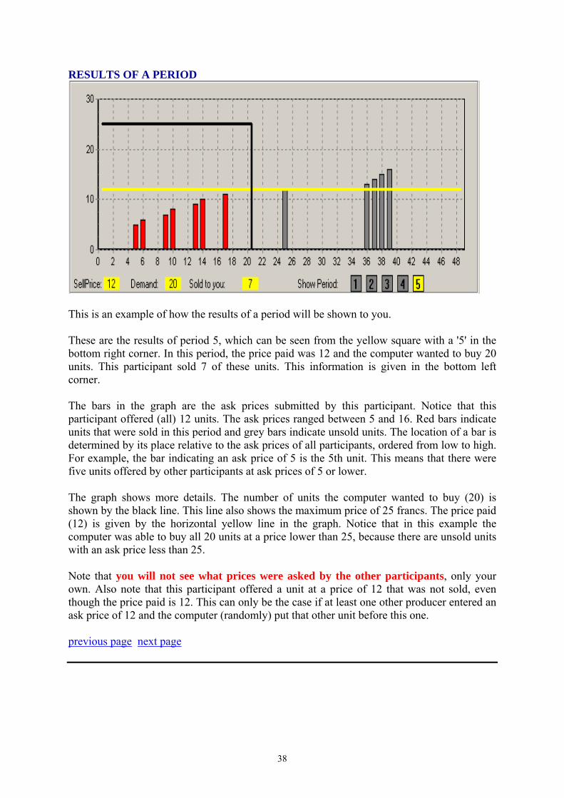
38

RESULTS OF A PERIOD

This is an example of how the results of a period will be shown to you. These are the results of period 5, which can be seen from the yellow square with a '5' in the bottom right corner. In this period, the price paid was 12 and the computer wanted to buy 20 units. This participant sold 7 of these units. This information is given in the bottom left corner. The bars in the graph are the ask prices submitted by this participant. Notice that this participant offered (all) 12 units. The ask prices ranged between 5 and 16. Red bars indicate units that were sold in this period and grey bars indicate unsold units. The location of a bar is determined by its place relative to the ask prices of all participants, ordered from low to high. For example, the bar indicating an ask price of 5 is the 5th unit. This means that there were five units offered by other participants at ask prices of 5 or lower. The graph shows more details. The number of units the computer wanted to buy (20) is shown by the black line. This line also shows the maximum price of 25 francs. The price paid (12) is given by the horizontal yellow line in the graph. Notice that in this example the computer was able to buy all 20 units at a price lower than 25, because there are unsold units with an ask price less than 25. Note that you will not see what prices were asked by the other participants, only your own. Also note that this participant offered a unit at a price of 12 that was not sold, even though the price paid is 12. This can only be the case if at least one other producer entered an ask price of 12 and the computer (randomly) put that other unit before this one. previous page next page

39

RESULTS OF A PERIOD

After everyone has entered and confirmed their ask prices, a graph like this is shown for each of the 5 periods. Each period is shown for a few seconds. After the 5th period, you will be able to review any period by clicking on the numbers in the bottom right corner. You will have to indicate that you have finished reviewing all of the information of a round by clicking on a 'Ready' button (not shown here). We will not proceed to the next round until everyone has indicated that they are ready. previous page next page RESULTS OF A PERIOD

Here you see the 'Ready' button where you can indicate that you have finished reviewing the periods of a round.

40

You also see a table summarizing the results of a round. This will appear after period 5 has been completed by the computer. The table has one row for each period. The first column gives the period. The second column (demand) shows the quantity that the computer wants to buy in that period. If the number is in black, it was able to buy all units. If it is in red, there were not enough ask prices smaller than or equal to 25. Under the header 'price' you will find the price paid per unit in that period. The number of units sold by you is given in the column 'sold'. Your production costs (the number sold times 5) are given in the column 'costs'. Finally, your profit in this period (the price multiplied by the number sold minus your costs) is given under 'profit'. Between the table and the 'Ready'-button, we give your aggregate earnings in this round. This is the sum of your profits in the five rounds. previous page next page AGGREGATE EARNINGS During the whole experiment, a window in the op left corner will keep track of the round and period you are in. It also gives your aggregate earnings in francs. At the end of the experiment, your francs will be converted into euros. This brings you to the end of the instructions. You may now take your time to reread parts of the instructions. When you are satisfied that you understand them, you can indicate to us that you are finished, by clicking the 'ready' button at the bottom of this screen. After that, you may still page through the instructions. However, when everyone has indicated that they are ready, we will move on to the practice rounds. previous page back to first page

41

Appendix 2 – Equilibria of the MUA

Treatments hsh and hsl:

Each seller has 12 units of capacity in these treatments. In hsh demand quantities have a

discrete uniform distribution from 30 to 35; the distribution is from 20 to 35 for hsl. No seller

is pivotal in these treatments. The MUA model with continuous price offers provides a

simple prediction for these treatments; any pure strategy Nash equilibrium (PSNE) yields

market clearing prices equal to marginal cost (c = 5). This prediction is driven by strong

incentives to undercut rivals price offers in the symmetric, high capacity treatments.

Our experimental design departs from the continuous price interval assumption by

specifying that price offers must be chosen from a set of discrete prices, P {5,6,…,25,26}.

When price offers are restricted to a set of discrete price offers the incentive to undercut is

weakened, since a discrete price cut may involve a significant loss of revenue for infra-

marginal units. Below we describe our derivation of equilibrium results for a discrete price

version of the MUA model for our symmetric, high capacity treatments. First we state two

lemmas that support our computations.

Lemma 1 – Consider a PSNE with market clearing price p> c at demand quantity ̅. Then

price offers for equilibrium strategies are less than or equal to p for all units.

Remark – If a player offers any units at a price above p then the player could increase their

expected payoff by lowering offers on those units to p. Such a deviation would not affect

their payoff for any demand realizations that yield price less than p. And such a deviation

would raise their expected payoff for demand realizations that yield price equal to p, since

offering additional units at p would increase the player’s expected sales for those demand

realizations.

There are two implications of Lemma 1. First, an aggregate supply function s(p) that is

consistent with PSNE strategies with market clearing price p> c at demand quantity ̅ must

specify s(p) = 4k (total capacity of sellers). Second, when testing whether a particular vector

of strategies with market clearing price p> c at demand quantity ̅ is a PSNE, it is sufficient

to check deviations with all offers less than or equal to p. This can dramatically reduce the

number of payoff function evaluations when numerically checking for best responses.

42

Lemma 2 – Consider any vector of PSNE strategies. There exists a vector of PSNE strategies

with exactly the same market clearing prices and payoffs for players such that the lowest

1 offers are equal to marginal cost.

Remark – The first part of the argument for Lemma 2 is that if there is any offer among the

lowest 1 offers that is equal to the lowest market clearing price, then a player making

such an offer would have an incentive to reduce the offer below that price. So PSNE

strategies must have the property that the lowest 1 offers are less than the lowest market-

clearing price. Furthermore, reducing the lowest 1 offers to marginal cost has no effect

on market clearing prices or players’ payoffs, and cannot increase the payoff associated with

a deviation by any player. The joint implication of Lemmas 1 and 2 is that the set of

aggregate supply functions consistent with a PSNE can be limited to a relatively small set,

given a maximum market clearing PSNE price.

In principle one could search for all PSNE of the game with discrete prices via a

numerical search procedure, since the game has a finite set of strategies, and payoffs can be

computed for all strategies. However, the strategy set is enormous; there are roughly 225

million non-decreasing supply functions for 12 units and 25 discrete prices. An exhaustive

search for vectors of mutual best responses over such a large strategy set is not

computationally feasible. Our approach for analyzing the game with discrete prices combines

computation with the lemmas stated above. The computational algorithm has several parts.

Step One: Fix a maximum market clearing price p associated with a possible PSNE vector of

strategies.

Step Two: Identify the set of strategies (i.e., non-decreasing offer schedules) that have

minimum offer c and maximum offer p.

Step Three: Identify the set of aggregate supply schedules that are potentially consistent with

a PSNE with maximum clearing price p. Note that these aggregate supply schedules must be

consistent with Lemmas 1 and 2.

Step Four: For each possible aggregate supply schedule (from step 3), check each possible

strategy (from step 2) to see whether it is (1) consistent with the aggregate supply schedule

and (2) a best response to the implied sum of rivals’ offers. Collect all of the strategies that

pass tests (1) and (2) for a given aggregate supply schedule. From this set of strategies, check

whether there is a combination of 4 strategies that sum to the proposed aggregate supply

schedule. Any such vector of 4 strategies is a PSNE with maximum clearing price p.

43

This algorithm will indicate whether or not there are any PSNE that are consistent with a

particular maximum clearing price p, and if PSNE exist, this approach will identify the set of

equilibrium strategies. Matlab programs were written to perform the computations. Results

are reported in the table below, for several values of p.

Computation Results hsl hsh p # strategies # PSNE max VWAP # PSNE max VWAP 6 13 1 5.75 multiple 6 7 91 0 - multiple 7 8 455 0 - multiple 7.52 9 1820 0 - 0 - 10 6188 0 - 11 18564 0 - For a maximum market clearing price of p = 6 (one tick above marginal cost) there are 13

possible supply strategies. For treatment hsl there is exactly one PSNE with p = 6. Each

player offers 6 units at price equal to 5 and 6 units at price equal to 6. There are no PSNE for

maximum clearing prices 7 through 9 for HSL. For treatment hsh there are multiple PSNE for

maximum clearing prices 6 through 8. The maximum VWAP for these PSNE is 7.52. For

clearing prices 9 – 11 there are no PSNE.

We have not computed the set of equilibria for p> 9 for hsl or for p> 11 for hsh. As p

increases both the number of possible supply schedules (step 2) and the number of possible

strategies (step 3) get larger. Treatment hsl has a larger number of possible aggregate supply

schedules for each p than hsh, so the computation time increases faster for HSL as p

increases.40 While we have not performed computations for higher market clearing prices, the

computations reported above are the basis for our conjecture that price cutting incentives are

strong enough to rule out PSNE with market clearing prices greater than p = 6 for hsl and

greater than p = 8 for hsh.

Treatment lsl:

The only equilibrium is in mixed strategies. By offering all of its capacity at the price cap, a

single seller can guarantee itself expected profit of, 40 Computations were run using Matlab on a MacBook Pro. The p = 9 computation for hsl ran for 22 hours; the p = 11 computation for hsh ran for 55 hours.

44

35

max

20

25 5 max 0, 45ld l j

E d s

,

where is the probability of each possible demand level for lsl. This expected profit is

a lower bound for a firm’s mixed strategy equilibrium profit. This bound on profit permits us

to bound a measure of expected equilibrium price.

Given the definition of in the main text, total expected equilibrium profit for the

four firms in the market is defined by:

35

20d

Total profit d p d c

.

Since each firm must earn at least in equilibrium, we have the following inequality:

4

This implies that:

4

and this permits us to place a lower bound on the volume weighted average price:

411.55

Treatments lsh and hah:

In lsh each seller has 9 units of capacity and demand quantities are d {30,31,…,35}, with

equal probabilities. Let seller j offer its entire capacity at the price cap; that is,

max 25srlkp p , for k = 1,…,9. Let sellers lj choose offers, 17sr

lkp , for k = 1,…,9. Then

the market price is 25 for each demand realization. Expected profit for seller j is,

max(25 5) 110j ll j

E E d s

.

Sellerslj earn the maximum possible profit for a seller in this environment:

1/16

( )p d

45

max25 5 180j lE s . Seller j has no incentive to defect since she would have to

reduce her offers to 17 or less in order to increase her quantity sold. Even if seller j sold her

entire capacity at a price of 17 her payoff would be 108, which is less than the payoff of 110

associated with the high price strategy. So the asymmetric strategies described above are

Nash equilibrium strategies; see Fabra, et al (2006) for more details. There are four pure

strategy, asymmetric equilibria of this type, with a different seller acting as the high price

seller in each equilibrium.

Any of the pure strategy equilibria for lsh involve a substantially lower payoff for the

‘high price’ player, relative to other players. Players may resist settling on asymmetric

strategies, and instead opt for symmetric mixed strategies. If a mixed strategy equilibrium

exists, then we can use the security profit, 110, to place a lower bound of 18.5 for

expected VWAP, just as we did above for treatment lsl.

In hah there are two small sellers, each with 5 units of capacity, two large sellers, each

with 19 units of capacity, and demand quantities are d {30,31,…,35}, with equal

probabilities. Suppose that one of the large sellers offers their entire capacity at the price cap.

This would ensure that the market price is at the price cap (25) for each possible demand

realization. If the other three sellers offer all of their units at prices less than or equal to 8, the

high price seller has no incentive to change their strategy. These strategies are a Nash

equilibrium. There are two asymmetric Nash equilibria for hah, with one of the large sellers

acting as the high price seller in each equilibrium.

46

Appendix 3 – Equilibria of the SFE Model

In the derivations for the SFE model we treat both price and quantity as continuous variables.

Treatments hsh and hsl :

There are no pivotal suppliers for these two treatments. Consider the profit for firm i

in the event that demand is d, given that rival firm j chooses a differentiable supply function

sj(p) for ji.If the clearing price is p and firm i supplies the residual demand, jj i

d s p

,

then its profit is:

,i jj i

p d p c d s p

We seek a supply function si(p) for firm i that has the property that the clearing price

maximizesi(p,d) with i jj i

s p d s p

, for each possible ,d d d . The necessary

conditions for an (interior) optimal price for d for each firm i yield a system of ordinary

differential equations for supply functions:

' ( )

( )i

jj i

s ps p

p c

For i = 1,…,4. There is a continuum of symmetric solutions to this system of the form:

(*) ̅

where 'p is a price parameter that can take on any value in the interval, max, ; 'c p p is the

market clearing price associated with equilibrium supply strategies in (*) at maximum

demand quantity, d . Figure 2 in the main text illustrates aggregate supply functions based on

the strategies in (*). Note that in the limit as 'p approaches c the supply strategy in (*)

converges to the Bertrand strategy of offering all units at marginal cost. There are also

asymmetric supply function equilibria [see Genc and Reynolds (2011)]; the set of aggregate

supply functions associated with these asymmetric equilibria coincides with the set of

aggregate supply functions associated with symmetric equilibrium strategies in (*).

Treatments lsh and lsl :

For these treatments any one of the sellers is pivotal for some or all demand quantities. When

pivotal suppliers are present a strategy of offering capacity at prices close to marginal cost

p

47

will not be a symmetric equilibrium strategy. If a seller’s rivals use strategies in (*) with 'p

close to c then the seller would prefer to offer all of their capacity at the price cap rather than

use strategy (*). Genc and Reynolds (2011) show that the symmetric supply function

strategies in (*) are equilibrium strategies for capacity constrained pivotal sellers for a

restricted set of 'p parameters. For treatment lsh the supply functions in (*) are equilibrium

strategies for 'p [21.7,25]; for treatment lsl the supply functions in (*) are equilibrium

strategies for 'p [17.7,25]. The equilibria associated with these price parameters are the

basis for the (volume weighted) average equilibrium price predictions that we provide in

Table 3 of the main text. As for the symmetric high-capacity treatments, there are also

asymmetric supply function equilibria.

Treatment hah:

In this treatment there are two small sellers (each with 5 units of capacity) and two large

sellers (each with 19 units of capacity). There are quasi-symmetric supply function equilibria

of the following form. The small sellers each offer their capacity at a low price (e.g., at or

near marginal cost). The two large sellers compete for the remaining residual demand (d –

10) by choosing supply functions that are increasing in price. By using arguments similar to

those used earlier in this Appendix one can show that there is a supply function equilibrium

in which each large seller i uses the linear strategy:

(A3.4) 12( ) 10

'i

p cs p d

p c

where the price parameter satisfies, 'p [11.9,25]. As in the other treatments there is a

continuum of equilibria.

48

References:

Abbink, K. and J. Brandts (2008), “24. Pricing in Bertrand Competition with Increasing Marginal Costs”, Games and Economic Behavior, 63, 1-31. Anwar, A. W. (1999), “The Case for a Discriminatory Pricing Rule in Competitive Electricity Pools”, Mimeo, Department of Economics, University of Edinburgh. Baldick, R. and W. Hogan (2002), “Capacity Contrained Supply Function Equilibrium Models of Electricity Markets: Stability, Non-decreasing Constraints, and Function Space Iterations”, University of California Berkeley, PWP-089 Working Paper, August 2002. Baldick, R., R. Grant and E. Kahn (2004), “Theory and Applications of Linear Supply Function Equilibrium in Electricity Markets”, Journal of Regulatory Economics, 25, 143-167. Bolle F. (2001), “Competition with supply and demand functions”, Energy Economics, 23,253-277. Borenstein, S. J. Bushnell and F. Wolak (2002), “Measuring Market Inefficiencies in California’s Restructured Wholesale Electricity Market”, American Economic Review, 92, 1376-1405. Brandts, J., P. Pezanis-Christou and A. Schram (2008), “Competition with Forward Contracts: A Laboratory Analysis Motivated by Electricity Market Design”, The Economic Journal, 118, 192-214. Brunner, Ch., J.K. Goeree, Ch. A. Holt, and J. O. Ledyard (2010), “An Experimental Test of Flexible CombinatorialSpectrumAuctionFormats”, American Economic Journal: Microeconomics , 2, 39–57. Cox, J., T. Offerman, M. Olson and A.Schram (2002), “Competition for vs on the Rails, a Laboratory Experiment”, International Economic Review,43, 709-735. Davis, D. and C. Holt (1993), Experimental Economics, Princeton University Press. Davis, D. and C. Holt (1994), "Market Power and Mergers in Laboratory Experiments with Posted Prices”, RAND Journal of Economics, 25(3), 467-487. Fabra, N., N.-H. von der Fehr and D. Harbord (2006), “Designing Electricity Auctions,” Rand Journal of Economics, 37, 1, 23-46. Falk, A. and J Heckman (2009), “Lab Experiments are a Major Source of Knowledge in the Social Sciences,” Science, 326, 535-538. Federal Energy Regulatory Commission (2007), 18 CFR Part 35 (Docket No. RM04-7-000; Order No. 697), June 21, 2007. Genc, T. and S. Reynolds (2011), “Supply Function Equilibria with Capacity Constraints and Pivotal Suppliers,” International Journal of Industrial Organization, 29, 432-442. Green, R. (1999), “The Electricity Contract Market in England and Wales”, Journal of Industrial Economics, 47, 1, 107-124. Holmberg, P., D. Newbery and D. Ralph (2008), “Supply Function Equilibria: Step Functions and Continuous Representations”, Electricity Policy Research Group WP#EPRG0829. Cambridge: University of Cambridge. Hortacsu, A. and S. Puller (2008), “Understanding strategic bidding in multi-unit auctions: a case study of the Texas electricity spot market”, RAND Journal of Economics, 39, 86–114.

49

Kagel, J. and A. Roth (2000), “The Dynamics of Reorganization in Matching Markets: A Laboratory Experiment Motivated by a Natural Experiment”, Quarterly Journal of Economics,115, 201-235. Klemperer, P. and M. Meyer (1989), “Supply Function Equilibria in Oligopoly under Uncertainty”, Econometrica, 57, 6, 1243-1277. Kremer, I. and K. Nyborg (2004), “Divisible Good Auctions: The Role of Allocation Rules”, RAND Journal of Economics, 35,147-159. Newbery, D. (1998), “Competition, contracts, and entry in the electricity spot market”, RAND Journal of Economics, 29, 4, 726-749. Newbery, D. (2002), “Problems of liberalising the electricity industry”, European Economic Review, 46, 919-927. Rahimi, A. and A. Sheffrin (2003), “Effective Market Monitoring in Deregulated Electricity Markets”, IEEE Transactions on Power Systems, 18, 2, pp. 486-493. Rassenti, S., V. Smith and B. Wilson (2002), “Using experiments to Inform the Privatization/Deregulation Movement in Electricity”, The Cato Journal, 22, 3, winter 2002. Rassenti, S., V. Smith and B. Wilson (2003), “Controlling Market Power and Price Spikes in Electricity Networks: demand-side bidding”, Proceedings of the National Academy of Science, 100, 5, 2998-3003. Reitzes, J., J. Pfeifenberger, P. Fox-Penner, G. Basheda, J. Garcia, S. Newell and A. Schumacher (2007), “Review of PJM’s Market Power Mitigation Practices in Comparison to Other Organized Electricity Markets”, Report by The Brattle Group for PJM Interconnection, LLC. Sefton, M. and P. Zhang (2010), “Divisible-good uniform price auctions: the role of allocation rules and communication among bidders”, University of Nottingham working paper. Sheffrin, A.(2001), “Critical Actions Necessary for Effective Market Monitoring”, Mimeo, Department of Market Analysis, California ISO. Sheffrin, A.(2002), “Predicting Market Power Using the Residual Supply Index”, Mimeo, Department of Market Analysis, California ISO. Staropoli C. and C. Jullien (2006), “Using Laboratory Experiments to Design Efficient Market Institutions: The Case of Wholesale Electricity Markets,” Annals of Public and Cooperative Economics, 77, 4, 555-577. Wolak, F. “An Assessment of the Performance of the New Zealand Wholesale Electricity Market”, Investigation report, May 2009, available athttp://www.comcom.govt.nz/BusinessCompetition/ Publications/Electricityreport/DecisionsList.aspx Wolfram, C. (1999), “Measuring Duopoly Power in the British Electricity Spot Market”, The American Economic Review, Vol. 89, No. 4.