pilot tests of an international definition of urban
TRANSCRIPT

Pilot tests of an international definition of urban – rural territories
Summary report
Publication prepared in the framework of the Global Strategy to improve Agricultural and Rural Statistics
December 2018

Pilot tests of an international definition of urban – rural territories
Summary report

Table of Contents Acronyms and Abbreviations .................................................................................. 6 Preface .................................................................................................................. 7 Acknowledgements ................................................................................................ 8 Introduction .......................................................................................................... 9 1. Comparison of the international categorization to national practices................. 13
1.1 Brazil .............................................................................................................. 14 1.2 Colombia ....................................................................................................... 15 1.3 Ethiopia ......................................................................................................... 16 1.4 France ............................................................................................................ 17 1.5 Malaysia ........................................................................................................ 18 1.6 Pakistan ......................................................................................................... 20 1.7 United States of America .............................................................................. 20
2. Main conclusions on the comparison and the way forward ............................... 23
2.1 Urban and rural as a continuum ................................................................... 23 2.2 Variables and criteria in country practices ................................................... 25 2.3 Discrepancies and mismatches in classifications .......................................... 26 2.4 Going forward with regard to the international definition ........................... 27
3. Assessment of the application of the definition to data collection and for indicators construction......................................................................................... 28
3.1 Census data ................................................................................................... 29 3.2 Survey data.................................................................................................... 30 3.3 Administrative records .................................................................................. 30
4. Feasibility assessment ...................................................................................... 31
4.1 Brazil .............................................................................................................. 31 4.2 Ethiopia ......................................................................................................... 31 4.3 France ............................................................................................................ 32 4.4 Malaysia ........................................................................................................ 32 4.5 Pakistan ......................................................................................................... 33 4.6 United States of America .............................................................................. 34
5. Main conclusions regarding the indicators reporting ......................................... 35 6. Going forward regarding data collection and indicators reporting ...................... 37

Annex 1. National Institutions and Focal Points .................................................... 39 Annex 2. Tests Protocol ........................................................................................ 40 Annex 3. Country Factsheet: Brazil ....................................................................... 51 Annex 4. Country factsheet: Colombia .................................................................. 54 Annex 5. Country factsheet: Ethiopia .................................................................... 58 Annex 6. Country factsheet: France ...................................................................... 61 Annex 7. Country factsheet: Malaysia ................................................................... 64 Annex 8. Country factsheet: Pakistan ................................................................... 67 Annex 9. Country factsheet: United States of America .......................................... 71 References ........................................................................................................... 74
List of Figures and Tables Figure 1. Rural Grid System vs DEGURBA, Malaysia. .................................................... 19 Table 1. Levels 1 and 2 of the conceptual schema of the refined urban–rural definition. ...................................................................................................................... 10 Table 2. Summary of Level 1 and Level 2 comparison in the countries. ...................... 13 Table 3. Population size and density, cut-off values in the US Census Bureau’s definition of urban areas. ............................................................................................. 21 Table 4. Subset of SDG indicators for pilot tests*. ....................................................... 28

6
Acronyms and Abbreviations CIESIN Center for International Earth Science Information Network CSA Central Statistical Agency, Ethiopia DANE Departamento Administrativo Nacional de Estadística, Colombia DEGURBA Degree of Urbanisation DG REGIO Directorate-General Regional and Urban Policy DOSM Department of Statistics, Malaysia EC European Commission FAO Food and Agriculture Organization of the United Nations GHSL Global Human Settlement Layer GSARS Global Strategy to Improve Agricultural and Rural Statistics GPW Gridded Population of the World HDC High Density Clusters IBGE Instituto Brasileiro de Geografia e Estatística (IBGE), Brazil INSEE Institut national de la statistique et des études économiques,
France JRC Joint Research Centre of the European Commission MGN Marco Geostatístico Nacional, Colombia MDC Moderate Density Clusters PBS Pakistan Bureau of Statistics OECD Organisation for Economic Co-operation and Development SDG Sustainable Development Goals SMOD Settlements Model USDA United States Department of Agriculture

7
Preface
A proposed internationally-consistent definition of urban–rural territories
characterizes settlements based on population size and density. The definition is
purely people-based and relies on a population grid with cells of one square
kilometer (km2). Its application has been tested in seven countries: Brazil,
Colombia, Ethiopia, France, Malaysia, Pakistan, and the United States. There
were two objectives of the test. First, it aimed to evaluate the definition in a
country-specific context and contrast its characterization of population
settlements with those currently in use domestically. Second, it sought to assess
the feasibility of countries’ employing the definition to report on a subset of
Sustainable Development Goals (SDG) indicators using existing data collections.
The test results show heterogeneity in the degree of congruence between
domestic classifications and those of the definition. To varying degrees, the
differences can be attributed to the use of legal, non-population based
administrative boundaries for classification, adoption of other thresholds to
separate the classes in the definition, and the imposition of additional non-
population criteria, such as economic activity and remoteness, in classifying
settlements. Nonetheless, all countries showed familiarity and agreement with
the definition’s portrayal of urban and rural as a continuum rather than as a
dichotomy and acknowledged the value of having a consistent definition for
international reporting and comparisons. As for indicator reporting, the major
constraints to using the definition at present are the lack of congruence between
the geography of statistical reporting and the areas in the classes of the definition.
This mismatch is most problematic for survey data, where statistical validity
depends on having the sampling strata line up with the definition’s classes. Going
forward, the increasing integration of geospatial and statistical information will
address many of the current impediments to applying and using the international
definition while countries continue to employ their own approaches to urban–
rural classification for domestic purposes.

8
Acknowledgements The European Commission, the Global Strategy for improvement of Agricultural
and Rural Statistics (GSARS) and the Food and Agriculture Organization (FAO)
would like to thank colleagues in national statistical agencies who so kindly
participated in the test of the definition. These were informal tests, performed in
addition to their regular duties, and the time it took to engage on these tasks is
greatly appreciated. The lead contacts in each country and their affiliation are
reported in Annex, though many analysts were involved in implementing the test
protocols and their contributions are much valued, as well. In Brazil, Claudio
Stenner was the lead; in Colombia, Angélica Maria Palma Robayo and Sandra
Liliana Moreno Mayorga; in Ethiopia, Aberash Tariku; in Malaysia, Manisah
Othman; in Pakistan, Munwar Ali Ghanghro; and in the United States, John
Cromartie. The collective efforts of these colleagues and of involved staff
ensured a robust evaluation of the usefulness of the definition in varied country
settings.

9
Introduction
In 2016, the Global Strategy to Improve Agricultural and Rural Statistics
(GSARS) and FAO joined a voluntary commitment (VC) comprised of the
Directorate-General Regional and Urban Policy (DG REGIO) of the European
Commission, the Organisation for Economic Co-operation and Development
(OECD) and the World Bank to develop a proposal for an internationally-
consistent classification of urban–rural territories. The proposed definition
characterizes settlements across the urban–rural continuum based on population
size and density. The definition is people-based and relies on a population grid
with cells of 1 km2. The grid is developed by the Joint Research Centre of the
European Commission within the Global Human Settlement Layer (GHSL)
project1. The Degree of Urbanization (DEGURBA+) is the conceptual schema
that applies globally to the population grids of the GHSL2. Hereinafter, the layer
with the urban-rural categorization is called SMOD/DEGURBA.
The context for this request is the ongoing emphasis of the United Nations
Statistics Division on the integration of geospatial and statistical information and
on the use of geospatial referencing in enumeration of the 2020 census3.
Moreover, the United Nations General Assembly has stipulated that the
Sustainable Development Goals (SDG) indicators be disaggregated by key
demographic categories and by geographic location4. While the use of geocoded
data and geographical information systems is not at present widespread among
countries, there is consensus that moving toward global adoption is a goal that
will enhance the value of statistics in a wide range of applications in the public
and private sector. The pilot test results shed some light on the challenges and
1 http://ghsl.jrc.ec.europa.eu/ 2 It can be freely downloaded here. The layer with the urban-rural categorization is called GHS-SMOD http://ghsl.jrc.ec.europa.eu/ 3 Principles and Recommendations for Population and Housing Censuses, available at https://unstats.un.org/unsd/demographic/meetings/egm/NewYork/2014/P&R_Revision3.pdf 4 UN General Assembly resolution 71.313, Work of the Statistical Commission Pertaining to the 2030 Agenda for Sustainable Development, 6 July 2017.

10
opportunities in applying the urban–rural definition in reporting SDG indicators
at the present time and in moving forward.
The refined urban–rural categorization delineates the urban versus rural areas to
capture the full settlement hierarchy in a nested system with increasing level of
disaggregation. A higher level of detail or disaggregation facilitates the analysis
and understanding of how variations in people’s circumstances and well-being
are based on the places where they live and permits the design of policies
meaningful to each reality. Table 1 below shows the first two levels of the urban–
rural characterization.
Table 1. Levels 1 and 2 of the conceptual schema of the refined urban–rural definition.
Level 1 Level 2
Code Description Rule Code Description Rule
Rural (RUR)
Rural grid cells
Cells with a population <=
300 or > 300 but outside moderate density clusters
(MDC)
10
Uninhabited permanent water surfaces
No population and less than 50% land area
11 Mostly uninhabited area
Population density between 0 and 50
12
Dispersed rural area
Population density between 50 and 300
13 Villages
Contiguous grid cells with population density of at least 300 and a cluster population between 500 and 5 000; excluding MDC;
Moderate density cluster (MDC)
Urban clusters
Contiguous cells with a density of
at least 300 residents per km2 and a minimum
population in the cluster of 5 000
22 Suburbs
Contiguous grid cells with a density of at least 300 residents per km2and a minimum cluster population of 5 000; excluding

11
cities (HDC) and towns
21
Towns
Contiguous grid cells with a density of at least 1,500 residents and a cluster population between 5 000 and 50 000; excluding cities (HDC);
High density cluster (HDC)
Urban centres
Contiguous cells with a density of at least 1 500 residents per km2 (or at least 50% built-up) and a minimum population in the cluster of 50 000. Gaps are filled and edges are smoothed
30 Cities Same as Level
1
Note: “Contiguous” refers to the 4 cells adjacent to each cell in the grid (cells that touch at the corners are not included).
DG REGIO, the JRC, the GSARS and FAO tested in the summer of 2018 this
refined definition in seven pilot countries. Having both Level 1 and Level 2 tested
in countries over the entire rural–urban continuum is expected to provide a more
systematic and robust presentation of the concepts towards an agreed
international definition and to help understanding the main constraints and
challenges countries might face in adopting it. These were informal analytical
tests, carried out with the kind cooperation of country statistical agencies.
Countries were not asked to take an official position on adoption of the definition
by their governments or by any international body.
Countries participating in the pilots are the following: Brazil, Colombia,
Ethiopia, France, Malaysia, Pakistan and United States of America (USA).
Countries vary widely by the distribution of their population as some have highly
concentrated versus highly dispersed settlement patterns. They also differ by
geographical features such as the heterogeneity of landscapes and of land cover
types, climate and topography. This variability accounts for areas that may have
pockets of settlements or may be entirely uninhabited, such as mountains or

12
glaciers. They also have diverse levels of development as they include both high-
and low-income countries, which in turn may correspond to distinctive patterns
of settlement density. Finally, the availability of relevant information also varies
significantly in the pilot countries: in some cases, socio-economic and
environmental data are only available by administrative unit whereas others
already have data systems available in a georeferenced format and fully
compatible with the cells of the population grid.
The objectives of the pilots were twofold.
1) The first aims at applying the urban–rural continuum in country-specific
context to compare and contrast its characterization of population
settlements with those currently in use domestically.
2) The second objective aims at assessing countries’ opportunities,
capacities and constraints to report a subset of core SDG indicators on
livelihoods and wellbeing using the proposed definition and existing data
and sources (e.g. Census, administrative sources, household surveys,
multipurpose survey, and others).
Countries were provided with an instructions protocol and with supporting
material including country factsheets and geo-spatial layers (Annex).
13
1 Comparison of the international categorization to national practices
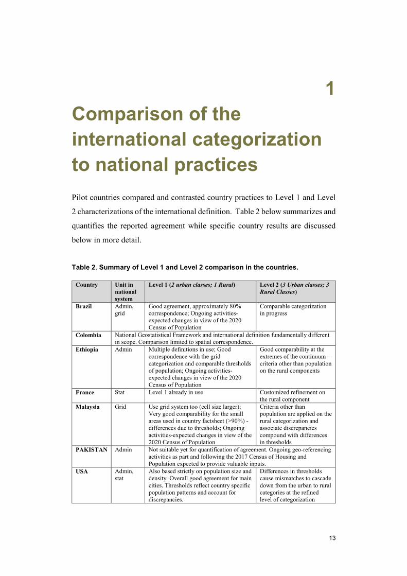
Pilot countries compared and contrasted country practices to Level 1 and Level
2 characterizations of the international definition. Table 2 below summarizes and
quantifies the reported agreement while specific country results are discussed
below in more detail.
Table 2. Summary of Level 1 and Level 2 comparison in the countries.
Country Unit in national system
Level 1 (2 urban classes; 1 Rural) Level 2 (3 Urban classes; 3 Rural Classes)
Brazil Admin, grid
Good agreement, approximately 80% correspondence; Ongoing activities-expected changes in view of the 2020 Census of Population
Comparable categorization in progress
Colombia National Geostatistical Framework and international definition fundamentally different in scope. Comparison limited to spatial correspondence.
Ethiopia Admin Multiple definitions in use; Good correspondence with the grid categorization and comparable thresholds of population; Ongoing activities-expected changes in view of the 2020 Census of Population
Good comparability at the extremes of the continuum – criteria other than population on the rural components
France Stat Level 1 already in use Customized refinement on the rural component
Malaysia Grid Use grid system too (cell size larger); Very good comparability for the small areas used in country factsheet (>90%) - differences due to thresholds; Ongoing activities-expected changes in view of the 2020 Census of Population
Criteria other than population are applied on the rural categorization and associate discrepancies compound with differences in thresholds
PAKISTAN Admin Not suitable yet for quantification of agreement. Ongoing geo-referencing activities as part and following the 2017 Census of Housing and Population expected to provide valuable inputs.
USA Admin, stat
Also based strictly on population size and density. Overall good agreement for main cities. Thresholds reflect country specific population patterns and account for discrepancies.
Differences in thresholds cause mismatches to cascade down from the urban to rural categories at the refined level of categorization

14
1.1 Brazil
Brazil currently applies for statistical purposes the dichotomy urban–rural. By
constitution, the 5 570 Brazilian municipalities are defined as urban, regardless
of their population size. Whereas the Level 2 categorization of the international
proposed method, does not currently find a direct correspondence in country
practices, an on-going work in preparation of the Demographic Census 2020
shows many elements of comparability with the refined categorization of Level
2. The Brazil Institute of Geography (IBGE) published in 2017 a preliminary
categorization5, which closely aligns methodologically to those applied to the
DEGURBA/SMOD grids. As part of this activity, the IBGE developed a 1 km2
statistical grid with data of total population and households derived from the 2010
Census. The definition of urban includes cells with at least 300 inhabitants per
km2 and at least 3 000 inhabitants in the cluster. Unlike the more restrictive rules
for cluster connectivity in the DEGURBA/SMOD grid, the preliminary
categorization considers all neighboring cells, including on the diagonal (8-conn
cells). Criteria for inclusion into the urban categories (both high and moderate
densities) are thus less stringent than in the international definition. This
discrepancy accounts for a larger share of the population (84%) defined as urban
in the Brazil system when compared with the international definition (79.5%).
Brazil reports that the new classification should coexist with the current one to
ensure comparability with past years. The new form of delimitation aims to
maintain the binary separation between the urban and rural categories but also
introduces subcategories to show the diversity of settlements of the territory. The
categorization aims to identify the territorial patterns that exist in the country
such as dispersed rural occupation, rural occupation in riverside, rural occupation
in planned settlements, rural occupation in villages, urban occupation,
metropolitan urban occupation and natural areas. Brazil preliminary categories
define the municipalities hierarchically taking into account their population size
as well as the road distance from the principal urban center in the upper urban
5 IBGE, 2017, Characterization and Classification of Rural and Urban Spaces in Brazil. As the categorization is in progress, this may differ from the final retained version.

15
hierarchy. The approach is thus comparable to the Level 2 of the international
definition as it categorizes the urban–rural continuum from the 1) Predominantly
urban municipality to 2)Adjacent intermediate municipality to 3) Remote
intermediate municipality, 4) Adjacent rural municipality and to5)Remote rural
municipality. Unlike the international categorization, it introduces an additional
criterion of remoteness from the main urban centers to categorize the rural
components.
1.2 Colombia
In Colombia, the National Administrative Department of Statistics (DANE) has
created and is updating the National Geostatistical Framework (Marco
Geostatístico Nacional – MGN), which is a system that allows the geo-
referencing of statistical information from censuses, sample surveys, derived
statistics, and administrative registers to their geographical location. It is
composed of geostatistical areas that support DANE calculations and
dissemination of statistics on population and built-up areas. The available level
of information includes the Country, Departments, Municipalities and classes
such as the Municipal Township (Cabecera Municipal), the Populated Center
(Centro Poblado) and rural area (Área Rural Dispersa) as well as other
geostatistical areas, bounded mainly by geographical and cultural features,
identifiable in the field.6 The Cabecera Municipal or Municipal Township refers
to a geographic boundary applied by DANE for statistical purposes, allusive to
the geographical area bounded by the census perimeter. The administrative
headquarters are located within, i.e. the town hall. The Municipal rest describes
the remaining municipal territories. It includes the Centros Poblados or
Populated Centers. This is a concept created by DANE for statistical purposes,
whose scope is the geographic location of population nuclei or population
settlements. A Populated Center corresponds to a concentration of at least 20
contiguous dwellings, neighbors or semi-detached houses.7 The Área Rural
6 For more information: https://geoportal.dane.gov.co/v2/?page=elementoMapaDane 7 DANE. Methodology for the Codification of the Political-Administrative Division of Colombia -DIVIPOLA-.

16
Dispersa8 is characterized by a sparse occupancy of the settlements and by the
predominance of agricultural and livestock activities.
The MGN does not explicitly articulates a distinction of the urban and rural
territories. Because the National Geostatistical Framework and the international
categorization differ in scope, a comparison between them was done, at a general
level, in terms of quantities, areas, population and density between the levels that
were equivalent or approximately coincident with each other. The comparison
suggests that there is no good degree of correspondence between the two systems;
therefore, it is not possible to draw conclusions on the suitability of the
international proposition to represent a categorization of the urban – rural
continuum in the country. Although the urban cells of the international
categorization coincide largely with 798 Municipal Townships of the 1,121
belonging to the MGN (71%); only 113 Municipal Townships (10%) have a
spatial coincidence with cells belonging to cities of the international
categorization. Cells belonging to the dispersed rural and mostly uninhabited
categories largely coincide with the Dispersed rural areas of the MGN.
Even though there are differences in the results obtained with respect to the
urban–rural classification and although DANE is not the official entity in the
country to define this concept, the desktop assessment in Colombia indicates that
methodologies maybe established to standardize the concepts worldwide
allowing international comparisons of relevant statistics and calculation of
sustainable development objectives.
1.3 Ethiopia
The Ethiopia Central Statistical Agency (CSA) defines, in its statistical system,
as urban centers all the administrative capitals and entities regardless of their
population size. These include the Regional capitals, Zone capitals, Woreda
capitals, Localities with Urban Dweller Associations, Municipal towns. It also
8 Available at: http://microdata.worldbank.org/index.php/catalog/490/download/14776

17
defines as urban all localities that do not belong to the above categories and that
have a population of 1 000 people or more, and whose inhabitants are primarily
(more than 50%) engaged in non-agricultural activities. On the other hand, all the
localities with population less than 1000 people are considered rural.9 Boundaries
are natural and human made features, which are identified by the local, zonal,
and regional administrative bodies. The national statistical system thus relies on
a categorization based on criteria other than the population size and density as in
the proposed international definition. Ethiopia also applies a categorization of the
capitals based on cut-off values of population that indicate a good
correspondence, if not directly quantifiable, between the national and
international system. The national system defines as Large and Medium cities
those having respectively 100 000 and more people and those with 50 000 to 100
000 inhabitants. Together, they would correspond to the Cities in the proposed
international definition. Small Capitals are those with a population size of less
than 50 000 inhabitants. These are expected to match well to the Moderate
Density cells of the urban clusters. The lower bound on the rural domain is 1 000
people. This also agrees well with the rural component of the international
definition, which however has a higher bound (maximum 5 000 in the cluster)
for the rural areas. It is worth noticing however that the country is preparing for
the forthcoming Census of Housing and Population. In this context, a new
categorization of the urban areas (and thus of the rural areas) is under
development.
1.4 France
In France, the National Institute of Statistics and Economic Studies (INSEE)
already applies the Level 1 of the DEGURBA. National practice expands the
rural component of the continuum and distinguishes further between thinly and
very thinly populated rural areas. Thus, the national system matches fully the
Level 1 – where the Densely populated area (cities) are those with at least 50%
9 Statistical Concepts and definitions, Central Statistical Agency of Ethiopia.

18
living in high density clusters, i.e. the cities; the Intermediate10 density areas are
those with less than 50% of population living in rural grid cells & less than 50%
of population living in high density cluster, i.e. towns and suburbs. The Thinly
populated areas (rural area) are those with less than 50% living in urban cells (1
and 2) & less than 50% living in very thinly cells. France also distinguishes the
Very thinly area (deep rural area) with at least 50% living in very thinly density
cluster. This distinction introduces criteria of distance from the main urban
centers and their economic influence. Nonetheless, the distinction is expected to
match closely to the refined categorization of the Dispersed rural areas and
Mostly uninhabited rural areas of Level 2 in the SMOD/DEGURBA conceptual
schema.
1.5 Malaysia
The Department of Statistics, Malaysia (DOSM) defines for statistical purposes
the urban areas based on i) the Gazetted area: areas under the jurisdiction of a
local authority that were classified based on their urban characteristics; ii)
Threshold of at least 10 000 people; iii) Economics activities - Built-up area: with
60 per cent of the population (aged 15 years and over) involved in non-agriculture
activities. In this categorization, agriculture activities are interpreted as common
part and proxy for rural social characteristics. Rural is the residual of urban. A
separate categorization is also in use in the country, which support the Rural Grid
System (cell size of 10 km2) of the Federal Department of Town and Country
Planning (PlanMalaysia). Figure 1 reports this national definition compared to
the SMOD/DEGURBA schema as from the country pilot.
10 Coinciding with “Moderate density cluster” as renamed in most recent versions of the conceptual schema.

19
Figure 1. Rural Grid System vs DEGURBA, Malaysia.
Source: Malaysia pilot test
Level 1 of the proposed international definition matches the national
categorization to reach over 90% of correspondence for the small areas that were
tested in the Malaysia test. As it moves to a refined categorization, Malaysia
introduces criteria other than only population size to include also the distance
from the town centres as well as land cover and land use aspects, which are
proxies for increasing rurality across the continuum. These criteria integrated
within the Village Grid System are used to identify gaps and links between
municipalities and rural areas arranged according to physical typography,
demographics and economics. This system determines the physical position of a
village and is able to solve the problem of the village boundaries. It assists the
design and setting of specific policies based on village characteristics and
according to their respective categories and needs. The application of criteria
other than population together with the observed differences in thresholds,

20
contribute to the discrepancies on the rural component of the continuum that were
observed between the national practice and the international definition.
1.6 Pakistan
In the 1981 census, the Pakistan Bureau of Statistics (PBS) moved away from a
population size-specific criterion to adopt instead an administrative criterion.
Urban areas and their boundaries are defined by official notification of the
respective provincial governments. Rural on the other hand encompasses all
population, housing and territory not included within an urban area. The country
test revealed a correspondence between the High Density Cluster (City) of Level
1 with the Major cities notified by the administration. The Moderate Density
Cluster would thus correspond to the rest of the urban area that is not a major
city. The rural grid cells of the proposed international definition would then
correspond to the residual of the urban areas and might be compared spatially to
the smallest revenue unit of the country. This corresponds to the “Mauza/Deh”
which is the term for Settled Rural Areas where as the term “Village” indicates
the Unsettled Rural Areas11. To date, the congruence between the national and
international methods could not be quantified. However, as part of the 2017
Population and Housing Census, the PBS produced geo referenced information
of the Enumeration Blocks (EB)12 applied to collect information on the urban
areas, and work is in progress to extend the coverage to the EB of the rural areas.
In the future, it will be then possible to measure the congruence between the two
methods.
1.7 United States of America
In the USA, the Department of Agriculture’s Economic Research Service (ERS)
compared the US Census Bureau’s definition of urban area to the international
11 Settled Rural Areas have proper measurements thatmay be identified through cadastral paper maps (massavies). Conversely, the Unsettled Rural Areasdo not have proper measurements (e.g. (KPK;- FATA,Tribal, Uper Dir, Lower Dir, Kohistan, Torgar. Balochistan: Awaran,WashuK, Makran Sherani etc). 12 The EB is the smallest unit of enumeration. It comprises on average 250 to 350 households.

21
proposed method. This US definition is strictly based on measures of population
size and density and on very small geographic building blocks– i.e. census tracts
and block groups–that are closer in size to the cells of the population grid of the
SMOD/DEGURBA. Table 3 below summarizes the thresholds of population size
and density applied in the US definition to characterize the urban areas, urban
clusters and the residual rural areas.
Table 3. Population size and density, cut-off values in the US Census Bureau’s definition of urban areas.
US Census Bureau’s definition of
urban areas
Criteria
Urbanized areas >= 50 000 people & pop. density >= 390/ km2
May contain suburban territory with pop. density >= 195/ km2
Urban clusters 2 500 – 50 000 people & pop. density >= 390/ km2
Rural < 2 500 people & pop. density < 195/ km2
As in the international proposed grid, cut-off values of both population size and
density should be met to match the inclusion in a given class. A comparison of
the two categorizations is therefore not straightforward. Nonetheless, the schema
shows an overall good agreement between the national categorization and Level
1 of the SMOD although the USA practice applies less stringent conditions to
define the urban areas given the lower cut-off value of population size (2,500
people as opposed to 5 000 people in the upper bound of the SMOD/DEGURBA).
As the focus moves towards the comparison with the Level 2 categorization,
mismatches become however significant. In general, ERS observed that cities,
towns and villages are much more narrowly defined in the proposed international
definition than in national practice. Differences in thresholds applied to the
distinction of the urban areas cascade down to the rural level and its refined
categorization. For instance, the country test reports that nearly 65 000 km2 of
territory that is characterized as urban (cities or towns) in the national definition,
falls in the Level 2 category of “Dispersed rural areas” and over 20 000 km2
correspond “Mostly uninhabited rural areas”. In general, the country pilot
observes that the thresholds of population density in the proposed international

22
method are set at a high level. This hinders a more adherent representation and
categorization of the sparser density pattern that characterizes the urban areas in
the USA.

23
2 Main conclusions on the comparison and the way forward 2.1 Urban and rural as a continuum
Heterogeneity in the geographical and socio-economic contexts of the pilot
countries likely contributes to the variability in national practices when defining
what territories are urban or rural. As noted in the field test reports of the United
States, the existence of multiple definitions reflects the reality that rural and urban
are multidimensional concepts, encompassing administrative, structural, and
economic constructs. Thus, and included within the same country (e.g. USA,
Malaysia), different definitions serve different research and policy applications.
Notwithstanding this heterogeneity, all countries showed familiarity with the
concept of urban and rural as a continuum rather than a dichotomy and
appreciated the refined categorization along the spectrum that is offered by the
Level 2 of the proposed international definition. Indeed, most of the countries
already adopt or are in the process of establishing national categorizations of the
urban–rural continuum for statistical purposes as well as for planning and fine-
tuning of relevant policies.
Examples of country categorizations that take into account this concept were
observed earlier in the text. Ongoing work in Brazil moves towards a refined
categorization of the rural domain, considering primarily the distance from the
urban domain as the main perspective. France already adopts the Level 1 of the
SMOD/DEGURBA. The national definition expands the rural component of the
urban–rural continuum to distinguish further between thinly and very thinly
populated rural areas. This further category accounts for the fact that the majority
of the settlement area in France is classified as rural cells according to the

24
international proposed system (country factsheet in Annex). France decided to
combine a functional and a morphological approach to separate the rural cells
within and outside the economic influence of the urban cores, i.e., those that offer
economic opportunities to the surrounding population. Interestingly, the national
practice in France focused on a refinement of the rural domain, there where Brazil
works towards a categorization of the more densely populated components of the
spectrum. This different emphasis finds a correspondence in the different results
of the international categorization in the two countries. Unlike France, the
SMOD/DEGURBA categorizes the Brazil population as primarily urban
(country factsheet in Annex).
A statistical grid supports the urban–rural characterization of Malaysia. Despite
the differences in applied cut-off values of population, this national statistical
system articulates a categorization of the urban–rural continuum that closely
resembles the Level 2 of the internationally proposed definition. Even in
countries such as Colombia and Ethiopia where current national definitions rely
on administrative units and legally prescribed entities, the categorizations
incorporate elements that describe aspects of the urban–rural continuum in the
national specific contexts. In Colombia, dispersed rural areas are identified by
sparse settlements, prevalence of agricultural activities, and limited availability
of services. In Ethiopia, the prevalence of agricultural income is part of the
definition for rural locality. In the USA test, the reported definition characterizes
the urban–rural continuum with a methodological approach that is similar to the
proposed international definition as it is essentially based on population. Diverse
definitions however coexist in national practices in support of different statistical
processes including the gathering of socio-economic data across the urban and
rural continuum.
Regardless of the technical differences, pilot countries share a common
understanding of the need for categorizing the degrees of urbanization and
rurality along the continuum. Pilot tests generally recognized that the Level 2

25
categorization of the SMOD/DEGURBA might contribute significantly to a
refined description of their urban and rural territories.
2.2 Variables and criteria in country practices
The country tests confirm expectations based on background analysis and
preliminary work and discussed in the UN Principles and Recommendations for
Population and Housing Censuses13. The traditional distinction between urban
and rural areas within a country has been based on the assumption that urban
areas, no matter how they are defined, provide a different way of life and usually
a higher standard of living than are found in rural areas. In many developed
countries, this distinction has however become blurred, and the principal
difference between urban and rural areas in terms of the living standards tends to
be the degree of population concentration or density. On the other hand, the
differences between urban and rural ways of life and standards of living remain
significant in developing countries, but even here, rapid urbanization has created
a great need for information related to different sizes of urban areas.
Country tests seem align well to these concepts. Typically, national practices
adopt the classification by size of locality to supplement the traditional urban–
rural dichotomy or even replace it there, where the major concern is with
characteristics related only to the population density along the continuum. Thus,
countries’ definitions look at the continuum from the sparsely settled areas to the
most densely built-up localities. However, pilot tests showed also that population
density alone is not a sufficient criterion in many countries (e.g. Colombia,
Ethiopia, and Malaysia) particularly where there are large localities that are still
characterized by a truly rural way of life. These countries indeed include to their
definitions additional criteria such as the prevalence of agricultural income,
distance and remoteness, land use aspects that are more distinctive than a simple
urban–rural dichotomy. The France test showed that, even in the industrialized
13Available at: https://unstats.un.org/unsd/demographic/meetings/egm/NewYork/2014/P&R_Revision3.pdf

26
countries, it was important to incorporate criteria other than the population size
of localities to categorize appropriately the specific pattern of settlements and
rural population.
2.3 Discrepancies and mismatches in classifications
Causes for the discrepancies that were observed between the national
categorizations and the international proposition may be separated in three main
groups. Firstly, differences are due to the statistical reporting unit that supports
the national practice. Typically, definitions that are based on prescribed legal
entities such as those observed in Colombia, Ethiopia and Pakistan agree less
with the population grid that underlies the SMOD/DEGURBA. The second
common reason for mismatches are the thresholds (cut-off values) in population
size. This was observed particularly in the Malaysia and USA tests and to some
extent in the preliminary categorization reported by Brazil. Thirdly, the inclusion
of additional criteria to national practices – typically applied to the categorization
in the rural domain –is another important cause for discrepancies. This was
observed in the country reports of Brazil, Ethiopia, France and Malaysia. Often,
all of these discrepancies are present in national categorizations of the urban–
rural continuum, as was observed for Ethiopia and Malaysia.
France has welcomed the greater level of categorization offered by the Level 2
of the SMOD/DEGURBA particularly in providing more detail to distinguish
between towns and suburbs. Categorization of the latter seems however
challenging. For instance, Brazil reported that the class “Suburbs” is not directly
meaningful in the national context and does not appear frequently in urban
concentrations. It also suggested that a more neutral labeling might help
understanding the correspondence in the national contexts. Also, Colombia,
Ethiopia and Pakistan definitions do not have a correspondence for this category.
USA test also pointed to the class “Surburbs” as source for mismatches and that,
in the country context, suburbs are typically identified with the cities or towns of
which they are a part. In this respect, very recent developments introduced at the

27
lowest hierarchical level (Level 3) of the SMOD/DEGURBA14made a refinement
in the category “Surburbs”, to account for the distance from the closest town.
This might partially address some of the concerns expressed by country pilots on
this category.
2.4 Going forward with regard to the international definition
As reported in Brazil, Ethiopia, Pakistan and Malaysia pilots, the 2020 round of
the Census of Housing and Population offers great opportunities for the
development of a geocoding and geo-referencing system at the national level
(UN, 2009)15. In general, efforts to build a national spatial data infrastructure
may be an opportunity for countries to integrate in country practices the
population grid and the urban–rural categorization offered by the
SMOD/DEGURBA. On a different angle, more recent and fine-grained census
data will contribute to the refinement of the population grid – reducing some of
the mismatches that were observed by countries, particularly in countries such as
Ethiopia and Pakistan where the input census data is outdated and rather
aggregated.
Countries also reported on the challenges presented by the integration to the
SMOD/DEGURBA system. There, where the availability of georeferenced data
is still limited, technical and financial constraints such as those mentioned in the
Ethiopia pilot might hinder, at least in the short term, this alignment. Legal
challenges were mentioned particularly by Pakistan given the political and
constitutional basis of the urban definition.
14 Communication from the Joint Research Centre, August 2018. 15 Handbook on Geospatial Infrastructure in Support of Census Activities. Available at: https://unstats.un.org/unsd/demographic/standmeth/handbooks/series_f103en.pdf

28
3 Assessment of the application of the definition to data collection and for indicators construction
The objective in this part of the pilot was the application of the urban–rural
definition in collecting the data necessary to construct the SDG indicators.
Countries were asked to focus on a subset (Table 4 is an excerpt from the
complete table in the Tests Protocol, reported in Annex) of Tier I indicators, those
for which the conceptual basis is clear, established methodology and standards
are available, and data are regularly produced by countries. The test protocol
requested an assessment of the feasibility of construction and calculation of a few
of these indicators as selected by each country.
Table 4. Subset of SDG indicators for pilot tests*.
*Excerpt from the complete table in Test Protocol, Annex.
Goals Selected SDG Indicators Tier Possible
Data Source
Available at what geographic level?*
Grid cells
Spatial units (enumeration area or municipality)
Cell size
Type of unit and
average surface or
population size
(Goal 1) End poverty
1.2.1 Proportion of population below the international poverty line, by sex, age, employment status, and geographical location (urban/rural)
I Household surveys

29
Because indicator construction depends on data collection appropriate to that use,
countries were asked to comment on the sources of data for a sub-set of these
indicators16: census, survey, or administrative record. The source of the data is
important because it determines how observations can be aggregated to align with
the classes in each of the two levels of the international definition. Grid cells are
individually classified and then viewed as groups of cells with the same
classification. These aggregations are compared against the boundaries of a
country’s own definition, as discussed earlier. The issue becomes how to align
data collected using different methods and geographies with these aggregates.
3.1 Census data
Census data are population-wide observations on individuals and households. In
the pilot countries, census-taking is done within enumeration units or blocks that
cover the entire or just settled regions, where each unit usually contains 150-300
households. Because a census is a universal enumeration, these household
observations can be aggregated as desired without concern for statistical validity.
On the other hand, survey data, as discussed below, are not so easily handled.
The method of aggregation must thus be addressed. If individual household data
are not georeferenced, they cannot necessarily be located in a particular
SMOD/DEGURBA grid cell. However, enumeration units may be
georeferenced. In that case, a list of households will be associated with each unit,
which can be located on a map. The boundaries of the census blocks can then be
superimposed on the SMOD/DEGURBA grid in which each cell is identified
uniquely with one of the three (Level 1) or six (Level 2) classes.
The class of the enumeration unit could be derived as that to which the majority
of cells belong. Depending on the area covered by each unit, the result could be
16 Countries were asked to identify a sub-set of 4-5 indicators for which data collection processes are already available in the country and, whenever possible, to select indicators that rely on diverse data collection methods.

30
more or less representative of the grid cells contained within it. However,
determination of the most representative class within an administrative unit by
reference to the area covered by each could produce counterintuitive results. In
very large spatial units, sparsely settled rural areas could account for much of the
geography and so by area the dominant class would be rural. However, if a large
densely settled city were contained within that unit, it would seem odd to
categorize the entire unit as something other than urban. The solution to this
dilemma lies in data collection according to the smallest possible geographic unit,
with geocoding at the household level being the ultimate refinement.
3.2 Survey data
Survey data are a sample drawn from a larger population, and the characteristics
of that population are estimated from the sample using statistical methodology.
Many SDG indicators are to be constructed on the basis of survey estimates using
sample stratification (see Table 4 above for examples). In the application of the
urban–rural definition, equal reliability is required for each of the three (or six)
classes. Therefore, the sampling strata would have to align with the areas
associated with each class.
3.3 Administrative records
Not collected for statistical purposes, these data may not cover all of a country’s
individuals or households or be representative of the characteristics of the
underlying population. If the records are geocoded to reflect location, then it may
be possible to aggregate what records there are according to Level 1 or 2 of the
SMOD/DEGURBA. Linking these records to statistical list or area frames could
facilitate their use in indicator construction.

31
4 Feasibility assessment Currently, this assessment was not possible for the pilot test of Colombia. 4.1 Brazil
At present, Brazil’s statistical reporting is based on administrative units that are
designated as either urban or rural. As discussed earlier, at Level 1, there is
approximately 80 percent correspondence of these units with the international
urban–rural definition. So, census and survey data might be used to construct
indicators at Level 1, although with some inconsistency in alignment with the
urban–rural definition’s geographies. With the refinements envisioned for the
2020 census, the congruence is expected to increase and reporting at Levels 1 and
2 will likely be feasible for census data. Survey data would have to be collected
according to the definition’s boundaries, and this would likely require larger
samples and more expense.
4.2 Ethiopia
Ethiopia evaluated the feasibility of indicators 3.c.1 (health worker density), 1.2.1
(proportion of population below poverty line), and 6.2.1 (proportion of
population using safely managed sanitation services). For the indicator on health
worker density, Ethiopia would rely on administrative reporting from each
facility in the country. The indicator on poverty would use data from its
Household Consumption and Expenditure Survey, and the indicator on sanitation
services would draw from its Demographic and Health Survey.
Ethiopia reports statistical data at the regional level. There are eleven
administrative regions, including two cities (Addis Ababa and Dire Dawa). As
discussed earlier, there is some degree of correspondence between Ethiopia’s
administrative units classed as cities and the urban areas in the Level 1 and 2

32
definitions. However, cities may be found within regions that also encompass
rural areas, so survey results at the regional level would not permit a distinction
between the urban and rural areas within the region. This situation constrains
indicator reporting at Levels 1 and 2.
4.3 France
France as noted is already using Level 1, with the added distinction of two classes
of rural instead of one. Therefore, its statistical reporting is aligned with the
international definition and so consistent indicators can be constructed. The
National Statistical Institute (Institut national de la statistisque et des études
économiques – INSEE) will release an update of the population grid at the
beginning of 2019 in which it will further extend from the two rural classes of
Level 1 to the four classes of Level 2 as in the international categorization. Thus,
good perspectives for the adoption of Level 2 are also envisaged.
4.4 Malaysia
Malaysia evaluated indicator 1.2.1 (population below poverty line), 3.2.1 (under
five mortality rate), and 4.6.1 (level of proficiency in literacy and numeracy).
Indicator 1.2.1 is collected using a household income survey, and 4.6.1 using
administrative data on skills assessment and national adult literacy. The indicator
on under five infant mortality would also be collected using administrative
records.
DOSM at present reports using units with administrative boundaries at the district
and state level. The Department defines enumeration blocks that are used in
census taking and in survey sampling. The major urban areas that Malaysia
identifies do align with the cities category of the international definition.
However, as discussed earlier, the agreement is limited for other classes because
Malaysia’s criteria for designating an area as rural includes more factors than
population size and density. Consequently, meaningful reporting at either Levels
1 or 2 is not currently feasible because of these mismatches.

33
In future, the Department expects to finish construction of the Malaysia Statistical
Address Register (MSAR), in which each living quarter will be assigned to a
unique ID and geocoded. At that point, it will be able to switch its methodology
from an area frame to a comprehensive housing unit frame. This will enable
census results to be aggregated in accordance with the international definition,
though survey data strata would still need to be aligned with the definition’s
classes.
4.5 Pakistan
PBS evaluated the feasibility of collecting data for nine of the sixteen selected
SDG indicators in Table 4, addressing all Goals in Table 4 including indicators
related to goals 15 and 16. Under Goals 15 and 16, indicators 15.3.1 and 16.6.2
are covered by PBS through Agriculture Census and Pakistan Social and Living
Standards (PSLM) district level survey respectively. The data sources for
monitoring of SDG indicators are surveys that mainly include those collected
under the PSLM initiative and cover Household Income& Consumption,
Education, Health, Employment, Water & Sanitation and Environment,. SDGs
are monitored by the following surveys conducted by PBS:
i. PSLM District level Survey;
ii. HIES Provincial Level Survey;
iii. LFS Provincial level Survey.
These surveys’ methodology samples from two strata, urban and rural. These
strata are defined by administrative units, where the urban domain corresponds
roughly to large-sized cities and then all other cities, and the rural strata is the
residual. In District level survey, each administrative district has been taken as
an independent stratum for four provinces. In Provincial level survey, each
administrative division has been taken as an independent stratum for the urban
domain. Conversely, for the rural domain, administrative district has been taken
as an independent stratum for Punjab, Sindh and Khyber Pakhtunkhwa (KP). For
the rural domain in Baluchistan, each administrative division has been taken as
an independent stratum. For Azad Jammu and Kashmir (AJK) and Gilgit-

34
Baltistan (GB) each administrative division has been taken as an independent
stratum for both urban and rural domains. The Major/Big cities are further
stratified in to low, middle & high-income groups but after Census 2017
information related to low, middle and high income groups is not available.
Hence, at this stage only urban and rural domains have been used. At present, as
discussed, the congruence between these units and those delineated in the
international definition has yet to be evaluated.
4.6 United States of America
The Economic Research Service (ERS) of the US Department of Agriculture
(USDA),considered that, if a grid-based harmonized definition were found to be
suitable for delineating urban categories (see its concerns in Section 2.7), then it
would be feasible to construct a range of socio-economic indicators using census
data, administrative sources, and household and multi-purpose surveys. ERS
uses grid-cell methodology and GIS techniques to combine data based on
different geographic building blocks. As an example of a possible strategy for
constructing SDG indicators, urban-area geography, block-level population data,
and a detailed road network map are downcast onto 0.5x0.5kilometer grid cells
to identify remote areas in the USA. ERS did note the limitations of this
approach, which include challenges in accurately allocating data reported using
relatively large geographic units to grid-based urban–rural categories. It
suggested that a better method would be to start with data collected using smaller
geographic building blocks, as those available from the US Census. However,
data on economic conditions, in particular, are collected at higher levels of
aggregation in surveys.
35
5 Main conclusions regarding the indicators reporting
A country’s ability to report indicators based on current data collections that are
consistent with the proposed international definition depends on the alignment of
its statistical data reporting with the classes in Levels 1 and 2. The possibilities
vary according to the source of the data to be used in constructing the indicator.
• With census data identified by enumeration block or geocode, indicators
could be reported according to the Level 1 urban–rural classes and for
Level 2 where enumeration blocks can be associated with the areas in
each class of the continuum. Because of the relatively good agreement
about urban areas between the proposed urban–rural definition and
countries’ current classifications, reporting of some indicators at Level 1
seems possible for census data. Also, population data could be reported
using this scheme. While Level 2 was endorsed as useful in policy
analysis and in program administration, not all countries in the pilot saw
reporting by Level 2 as immediately feasible. Without geocoded
household or census block data, breaking existing data into smaller
aggregates could not be done according to the six categories. France
reported that an aggregated four levels might be possible. Brazil
suggested it might be able to report at Level 2 for census data. The United
States also believed it could report some indicators at Level 2 but that, in
some cases, down casting from larger survey units would be necessary
and result in a loss in accuracy.
• With survey data, reporting indicators using the definition appears at
present problematic for most countries, especially for Level 2. To achieve
consistency with the definition, data collection would need to be aligned

36
with the geography appropriate to each class in order to produce
statistically valid results. Moving to align survey sampling frames with
the classes in the definition would require changes in statistical strategies
across most countries. While the Level 1 definition may compare
reasonably well to individual country designations of urban and rural
territory, the matches are not exact. Either sample strata must be aligned
with the definition or a judgment must be made that reporting according
to existing strata is acceptable. For Level 2, alignment of the definition
classes and strata may well require more extensive sampling in order to
produce statistically reliable results over a larger number of smaller
geographies. The costs of data collection would be increased
accordingly, a potential barrier to the use of the more highly
disaggregated Level 2 definition.
• With administrative data, geocoding of each observational unit would be
necessary for alignment with the definition’s classes. To do so would
likely have to be supported by a national geocoded address file. Malaysia
currently has one under construction, but it is not clear this work is
underway in any other country for use in statistical reporting.

37
6 Going forward regarding data collection and indicators reporting Using Level 1 to report SDG indicators would be a move toward consistency on
a global basis and therefore represent an improvement over the status quo.
However, in the immediate future, there would not likely be precise alignment of
the reporting with the urban–rural definition based on the SMOD/DEGURBA
cell classes. The test results show that countries can roughly align their internal
urban definitions with SMOD, which would still yield results that are more
comparable on an international basis, especially for indicators based on census
data. Level 2 is acknowledged as making meaningful distinctions across the
urban–rural continuum. However, capability to align census and especially
survey data with the more refined classes is not found in all countries. In this
more detailed context, the question of aggregation of existing data to fit the
classes has to be confronted on a county-by-country basis. Survey frames by
geography vary across countries, as do the classifications according to the
definition. In its principles for censuses, the UN Statistical Division has
identified the need to move in the direction of small area reporting (see footnote
3). Having smaller reporting units would facilitate adoption of the Level 2
classifications by reducing the size of geographical aggregates that may contain
different numbers of cells in different classes, complicating the determination of
the appropriate class to which the large unit belongs.
The pilot tests demonstrate that, at least for the immediate future, there will be
variability in the geographic resolution of each country’s data collection and
indicator reporting. Those differences should be recorded as a means of assessing
data quality and as a resource for analysts. With adoption of a global urban–rural
definition, it may be possible to assess each country’s reporting against that

38
standard. The point would not be to say which reporting is “correct” and which
is not, but to allow characterization of the sensitivity of global totals to variability
in definitions across countries.

39
Annex 1. National Institutions and Focal Points
Pilot Country
Institution Lead contact Email
Brazil Instituto Brasileiro de Geografia e Estatística (IBGE)
Mr. Claudio Stenner, Geography Coordinator
Colombia
Departamento Administrativo Nacional de Estadística (DANE)
Ms. Angélica Maria Palma Robayo, Coordinator Cooperation & International Relation Office
Ms. Sandra Liliana Moreno Mayorga, Directora Técnica, Dirección de Geoestadística
Ethiopia
Central Statistical Agency (CSA)
Ms. Aberash Tariku, Deputy Director General, Data Quality and Standard Coordination
France Institut national de la statistique et des études économiques (INSEE)
Mr. David Levy, Chef de pôle analyse territoriale, Région de Marseille
Malaysia Department of Statistics Malaysia (DOSM)
Ms Manisah Othman, Principal Assistant Director, Agriculture and Environment Statistics Division
Pakistan Pakistan Bureau of Statistics (PBS)
Mr. Munwar Ali
Ghanghro, Director
United States of America
Economic Research Service, US Department of Agriculture (USDA)
Mr. John Cromartie, Geographer

40
Annex 2. Tests Protocol
Paragraphs follow the numeration as in the original document. PILOT-TESTING AN URBAN/RURAL DEFINITION AND ITS APPLICATION FOR REPORTING SDG INDICATORS
1. Overview
A harmonised definition of urban and rural areas is important for making cross-
country comparisons of progress towards the Sustainable Development Goals
(SDGs) and for meeting the associated rural policy objectives. Leveraging the work
already dedicated to the SDGs, such a definition may also support national processes
thus ensuring efficient use of limited resources.
Consultation with country experts has led to a consensus about the value of adopting
such a definition for the purposes of international comparisons, and especially with
respect to SDG indicators. The proposed internationally comparable definition is
not intended to replace existing national schemas but rather to supplement them.
Countries will always retain and use their own definitions based on administrative
units or cultural and traditional political boundaries or other considerations. Still, in
this test, it will be useful to know whether the proposed definition has value in
national context and applications – for instance in supporting the design of data
collection mechanisms amongst other considerations.
The urban-rural definition presents a continuum that characterizes settlements
based on population size and density. This definition is thus people-based. This
continuum allows delineation of Urban versus Rural areas and makes it possible to
distinguish between Cities, Towns and Suburbs in densely settled urban areas and
among Villages, Dispersed areas, and Mostly uninhabited areas in thinly populated
areas. This higher level of detail or disaggregation facilitates the analysis and
understanding of how variations in people’s circumstances and well-being are based
on the places where they live and to design policies meaningful to each reality.

41
The spatial population grid that underlies the definition assigns population to cells
of uniform size across the landscape. These can then be aggregated using any
administrative or political boundaries that have significance in domestic contexts,
but they work best with small units.
This pilot test is a desktop exercise. This will help to save resources and to minimize
the efforts required.
• For the urban/rural definition, the principles used in its design promote
cost effective implementation. The method proposed for an international
definition is globally applicable, feasible with input data currently available
free of charge, and adaptable when more refined data become available. This
activity builds momentum as several organizations FAO, GSARS, the
European Commission, the World Bank, and the OECD closely collaborate
to provide a platform that ensures consistency between international urban
and rural definitions.
• For the key indicators, the set can be selected by your institute to leverage
the resources currently devoted to producing the SDGs indicators. The
value-added for countries is the context provided on urban and rural
development, so that the SDG indicators can be placed in domestic use, in
addition to meeting international reporting requests.
The pilot exercises will inform a judgment about the extent to which this
effort at parsimony has been successful. Cost-effectiveness is but one criteria
by which the definition and indicators should be evaluated. Their value in
domestic decision making and in international reporting is equally, if not
more, important. For instance, the proposed people-based definition may
support the design of data collection efforts.
2. What are the objectives
In the context above, these pilot tests have two main objectives:
1) The first aims at applying the urban/rural continuum in country-specific
context to compare and contrast its characterization of population settlements with
those currently in use domestically.

42
2) The second objective aims at assessing countries’ opportunities, capacities
and constraints to report a subset of core SDG indicators on livelihoods and
wellbeing using the proposed definition and existing data and sources (e.g. Census,
administrative sources, household surveys, multipurpose survey, and others).
3. Technical specifications of the urban/rural definition
The definition of urban/rural areas applied to this pilot testing is based on the Degree
of Urbanisation or “DEGURBA”17 concepts and models developed by the European
Commission.
The DEGURBA relies on a population grid with cells of 1 square kilometre. The
population grid is developed by the Joint Research Centre of the European
Commission within the Global Human Settlement Layer project18. The DEGURBA
is applied to the population grid19. Table 1 explains what thresholds are used to
assign each grid cell to one the classes in this urban -rural typology. This means that
all areas, inhabited or not, cities and towns, rural and suburban places are classified.
The refined urban-rural categorisation subdivides the three main classes to capture
the full settlement hierarchy. Table 1 shows the subdivisions created by level two.
• At Level 1, the DEGURBA distinguishes Urban centres (which define
cities); Urban clusters (which define towns and suburbs); and Rural cell
(which define rural areas);
• At Level 2 it divides the rural cells into Mostly uninhabited rural, Dispersed
rural areas and Villages. It splits the Towns from the Suburbs, which are a
single class at Level 1. The Cities are not subdivided.
It should be noted that the rural categorization is developed from the best available
data globally. Higher spatial resolution data, more detailed and updated information
17http://ec.europa.eu/eurostat/web/degree-of-urbanisation/background 18http://ghsl.jrc.ec.europa.eu/ 19 It can be freely downloaded here. The layer with the urban-rural categorisation is called GHS-SMOD http://ghsl.jrc.ec.europa.eu/

43
on human population and detailed statistics on the actual use of the built-up areas
will overcome current data constraints, when available.
Table 5. Levels 1 and 2 of the conceptual schema of the refined urban-rural
categorisation
LEVEL 1 LEVEL 2
Code Description Rule Code
Description
Rule
Rural (RUR)
Rural grid cells
Cells with a population <= 300 or > 300 but outside moderate density clusters (MDC)
10
Uninhabited permanent
water surfaces
No population and less than 50% land area
11 Mostly uninhabited area
Population density between 0 and 50
12
Dispersed rural area
Population density between 50 and 300
13 Villages
Contiguous grid cells with population density of at least 300 and a cluster population between 500 and 5,000; excluding MDC;
Moderate density cluster (MDC)
Urban clusters
Contiguous cells with a density of at least 300 residents per square km and a minimum population in the cluster of 5,000
22 Suburbs
Contiguous grid cells with a density of at least 300 residents per sq km and a minimum cluster population of 5,000; excluding cities (HDC) and towns

44
21
Towns
Contiguous grid cells with a density of at least 1,500 residents and a cluster population between 5,000 and 50,000; excluding cities (HDC);
High density cluster (HDC)
Urban centres
Contiguous cells with a density of at least 1,500 residents per square km (or at least 50% built-up) and a minimum population in the cluster of 50,000. Gaps are filled and edges are smoothed
30 Cities Same as
Level 1
Note: Contiguous refers to the 4 cells adjacent to each cell in the grid (cells that touch at the corners are not included).

45
Figure 1. Summary representation of refined urban-rural categorisation
Figure 2. Refined categorisation of rural cells in the population density grid
4. Key questions
The pilot testing should cover both the Level 1 and Level 2 classifications.
Comparing the definition with current domestic practices is intended to provide
insight into feasibility of use in international reporting and the value it may have in
a domestic context. The first questions concern the application of the definition
Small Medium Large500-5,000 5,000-50,000 >50,000
High density >1500 Dense urban cluster Urban centre
Moderate density 300-1500
Moderately dense, urban cluster
Low density 50-300Low density
rural grid cells
Very low density
<50Very Low
Density Rural grid cells
Urban clusters Urban centresRural grid cells
Not applicable
Areas outside settlementsSettlements by population size
Cel
l lev
el c
rite
ria
resi
dent
s pe
r sq
km
Rural cluster

46
itself, and the next ones explore how the definition can be used to organize statistics
for reporting for internationally-comparable SDG indicators.
• How does the Level 1 urban and rural definition compare to the national
urban-rural definition(s)?
• Do the more refined classes in Level 2 provide helpful distinctions about
where the population lives and in what circumstances? In particular, does
having a consistent people-based classification of settlements across the
country facilitate policy and program analysis?
• What would be the main constraints (institutional, technical, and financial)
for this Level 2 definition to be applied as a valid categorization?
• How could the definition be applied to existing data to construct a few SDG
indicators as demonstrations? Is georeferenced data used in indicator
construction currently available? Are there plans to adopt georeferencing in
sampling and collecting data?
Based on these questions, the testing may be subdivided in two complementary
parts: the evaluation of the rural definition with respect to current national practices
(section 5 in this document) and the evaluation of its application in the context of
developing key indicators (section 6).
5. Evaluation of the definition
Specific results of the application of the proposed definition in your country are
provided together with these instructions. Thus, based on the evaluation of these
results and comparison to national practices:
a) Please indicate how the Level 1 and Level 2 categorisation in urban and rural areas
differ from national practices. Are differences due to the identified thresholds?
b) A key aspect of the evaluation is to understand the value of the refined Level 2
classes in your country. Please review the thresholds and rules applied in the
categorisation of the urban and rural areas and compare them with those currently
in use in the national context. If applicable, could you prepare a corresponding

47
table between urban and rural categories in use in your Country and the proposed
Level 2 categorisation?
c) Please also indicate to what extent the method appears to identify rural areas at
the expense of urban centres and clusters and/or if the opposite occurs. Note
that, with the proposed definition, the assignment of rural to urban (or urban to
rural) areas may occur at Level 1, the highest hierarchical level (urban and rural),
as well as between categories of the same type (e.g. Villages that are coded as
Dispersed rural areas) in Level 2 (see Table 6).
Table 6. Mismatches in detection of rural and urban areas
Under-detection Over-detection
URBAN
Cities Some urban are missing Some rural are included
Towns and Suburbs
RURAL
Villages
Some rural areas are missing
Some urban areas are included as rural
Dispersed rural areas
Mostly inhabited areas
d) Please indicate to what extent the use of the urban/rural continuum would be
valuable in domestic policy decision making and analysis.
6. Assessing the application of the definition
The objective of this section is your assessment of the application of the proposed
definition of urban and rural areas in constructing indicators and in data collection.
Here, the emphasis is on Tier One indicators, those for which the conceptual basis
is clear, established methodology and standards are available, and data are regularly
produced by countries. Calculation of the specific indicator values is not needed;
instead an assessment of the feasibility of construction and calculation is sought.
The following list of key indicators of wellbeing are drawn from the existing SDG
set. Metadata (as of June 2018) are available from download from
https://unstats.un.org/sdgs/metadata/.

48
Table 7. Subset of SDG indicators for assessing the application of the definition
Goals Selected SDG Indicators Tier Possible Data Source Available at what geographic level?*
Grid cells Spatial units (enumeration area or municipality)
Cell size
Type of unit and
average surface or
population size
(Goal 1) End poverty 1.2.1 Proportion of population below the international poverty line, by sex, age, employment status, and geographical location (urban/rural)
I Household surveys
(Goal 2) End hunger 2.1.2 Prevalence of moderate or severe food insecurity in the population, based on the Food Insecurity Experience Index (FIES)
I Household surveys
(Goal 3) Ensure healthy lives
3.2.1 Under five mortality rate I Households surveys, administrative records
3.c.1 Health worker density and distribution I
Census, labor and employment surveys, administrative records
(Goal 4) Ensure inclusive and equitable quality education
4.1.1 Proportion of children and young people: (a) in grades 2-3;
(b) at the end of primary; and (c) at the end of lower secondary achieving at least a minimum proficiency level in (i) reading and (ii) mathematics, by sex
II Cross-national learning assessments
4.6.1 Percentage of population in a given age group achieving at least a fixed level of proficiency in functional (a) literacy and (b) numeracy skills, by sex
II Skills assessment and national adult literacy surveys
(Goal 6) Ensure availability of water and sanitation
6.1.1 Proportion of population using safely managed drinking water sources
I Household surveys, administrative records
6.2.1 Proportion of population using safely managed sanitation services, including a hand-washing facility with soap and water
I Household surveys, censuses
(Goal 7) Ensure access to energy
7.1.1 Proportion of population with access to electricity I Household surveys
7.1.2 Proportion of population with primary reliance on clean fuels and technology
I Household surveys
(Goal 8) Promote economic growth
8.3.1 Proportion of informal employment in non-agriculture employment, by sex
II Household and labor surveys

49
*Both grid and area units may be applicable.
Your Institution is kindly requested to identify a subset of 4–5 indicators for which
data collection processes are already available in the country. Whenever possible, it
would be ideal to select indicators that rely on diverse data collection methods (e.g.
Census, administrative sources, household surveys, multipurpose survey, and
others).
A key issue concerns aggregation of grid cells into the administrative or political
units that define the geographical areas over which data are collected. If data are
not georeferenced, they cannot necessarily be located in a particular grid cell. In that
case, the boundaries of a census enumeration unit, for example, could be overlaid
on the underlying settlement grid cells, and the classification of that group of cells
could be derived as the class to which the majority of cells belong (see Country Fact
Sheet). Depending on the area covered by each administrative unit, the result could
be more or less representative of the grid cells contained within it. A census unit
could contain all the same class (say, suburb) or could have more than one class (say,
town and suburb).
In the context of the definition, this part of the evaluation seeks to answer the
following questions:
8.5.2 Unemployment rate, by sex, age and persons with disabilities
I Household and labor surveys
(Goal 9) Build infrastructure, promote industrialization, foster innovation
9.c.1 Proportion of population covered by a mobile network, by technology I
Information and communication ministry data collected from internet providers
(Goal 11) Make cities and human settlements inclusive, safe, resilient and sustainable
11.6.2 Annual mean levels of fine particulate matter (e.g. PM2.5 and PM10) in cities (population weighted)
I Ground measurements monitoring networks, satellite remote sensing, topography, population
(Goal 15) Protect ecosystems, manage forests, combat desertification, halt land degradation, halt biodiversity loss
15.1.2 Proportion of important sites for terrestrial and freshwater biodiversity that are covered by protected areas, by ecosystem type
I
Inventories and surveys, remote sensing observations
(Goal 16) Significantly reduce all forms of violence and related death rates everywhere
16.1.1 Number of victims of intentional homicide per 100,000 population, by sex and age
I a) Criminal justice system; b) Public health/civil registration.

50
a) What data collection method are used for each selected indicator? Are these
indicators all relying on the same national definition of urban and rural areas?
If not, please specify how these differ. Is your Institution the one primarily
responsible for the collection of the selected indicators?
b) What would be the opportunities to apply the Level 2 definition for each
particular indicator?
c) What would be the main constraints in apply the Level 2 definition to each
data process? Would these constraints be of technical, financial, or of
institutional nature?
7. Supporting material
For each country participating in the testing, a factsheet is provided jointly to these
instructions to facilitate the quantitative and qualitative components of the
evaluation. Additional material will include:
a) Country Fact Sheet with results from the categorisation;
b) Interactive visualisation of categorisation in the country in Google Earth
(KMZ files) and instructions for visualisation (1 page).

51
Annex 3. Country factsheet: Brazil
Introduction This country summary is provided to support the assessment of an international definition of urban and rural areas by National Statistical Institutes. The goal of this assessments is to see whether the proposed definition and its categorisation accurately captures a country’s rural and urban areas.
Please note that inaccuracies in this country summary may be due to data quality. The results presented here are based on a combination of two data sources: population and built-up areas. The method ensures greater comparability and a harmonization of spatial concepts. The urban and rural characterisation can be applied to other data (e.g. census updates, better spatial resolution) that may improve the available classification of both rural and urban components.
The population source data are collected by the Center for International Earth Science Information (CIESIN) mostly from the National Statistical Offices. For Brazil, baseline data source are summarised in Table 1.
Table 8. Summary of the population data used by CIESIN for Brazil
Country Highest administrative level used
Number of units (polygons)
Population year
Population Source type
Brazil 5 316,461 2010 Final Census Population source citation The Brazilian Institute of Geography and Statistics (IBGE), Synopse do Censo Demografico 2010, ftp://ftp.ibge.gov.br/Censos/Censo_Demografico_2010/Sinopse/Agregados_por_Setores_Censitarios/, Accessed 07/05/2011.
Built-up areas are detected by the European Commission's Joint Research Centre using the Global Human Settlement Layer to define a Degree of Urbanization (DEGURBA). The DEGURBA classification schema is described in: http://ec.europa.eu/eurostat/web/degree-of-urbanisation/background. This classification in further refined into 6 classes instead of 3 (see the Global Human Settlement Layer or “GHS-SMOD” by the Joint Research Center of the European Commission – http://ghsl.jrc.ec.europa.eu/).
The degree of urbanisation has three classes based on three types of grid cells:
1. Rural grid cells is as all grid cells with a population density of less than 300 residents per square km and other cells that are outside an urban cluster.
2. An urban cluster consists of contiguous cells with a density of at least 300 residents per square km and a minimum population in the cluster of 5,000.
3. An urban centre consists of contiguous cells with a density of at least 1,500 residents per square km and a minimum population in the cluster of 50,000.

52
These three classes of local spatial units are defined using the three types grid cells as following:
1. A rural area has the majority of its population in rural grid cells.
2. Towns and suburbs have the majority of their population in an urban cluster (and it is not a city).
3. A city has the majority of its population in an urban centre.
Urban areas consist of cities, towns and suburbs. Please note that in some countries, the intermediate category ‘towns & suburbs’ is considered as part of the rural domain. The refined degree of urbanisation has six classes. It splits the towns from the suburbs. The rural areas are divided into villages, dispersed rural areas and mostly uninhabited areas.
Figure 2. Refined urban-rural categorisation – São Paolo, Brazil
Definitions: Rural grid cells (1 sqkm) include low density population cells
Mostly uninhabited _1 (pale green): Grid cells with a density below 50 residents per sq km; Dispersed rural areas_2 (bright green): Grid cells with a density between 50 and 300 residents per sq km; Villages_3 (dark green): Contiguous grid cells with population density of at least 300 and a cluster population between 500 and 5,000; excluding urban clusters;
Urban cells (1 sqkm) include urban clusters (or moderate density clusters) and urban centres (or high density clusters)
Suburbs _4 (yellow): Contiguous grid cells with a density of at least 300 residents per sq km and a minimum cluster population of 5,000; excluding cities and towns; Towns_5 (orange): Contiguous grid cells with a density of at least 1,500 residents and a cluster population between 5,000 and 50,000; excluding cities; Cities_6 (dark red): Contiguous grid cells with a density of at least 1,500 residents and a cluster population of at least 50,000;

53
Figure 3. Country results for Brazil based on the refined urban-rural categorisation
Table 9. Distribution of population by the refined urban-rural categorisation, example for three administrative zones – Minas Gerais, Brazil*
Administrative unit (Level 2)**
Mostly uninhabited
Dispersed rural areas Villages Suburbs Towns Cities Total
Population Belo Horizonte 0.0% 0.1% 0.0% 0.3% 0.3% 99.3% 2,491,174
Contagem 0.1% 0.3% 0.1% 1.9% 1.3% 96.2% 639,437
Sabará 0.9% 2.0% 2.5% 12.7% 41.9% 39.9% 144,822 *FAO calculations based on the Global Administrative Areas (GADM version 3.6); the refined urban-rural categorisation (v9s10C, 2015 results) and the population grid (GHS_POP_GPW41MT_GLOBE pre-Release version 2018); **Corresponding spatial representation is shown in Figure 3.
Figure 4. Spatial representation of example in Table 2 – Minas Gerais, Brazil
Notes about data:
In case of cross-border settlement areas, only population and surfaces estimates related to the Country are considered in this summary. The summary includes results from automatic data analytics workflows including global best available satellite data records collected by Earth Observations and census data made available by National Statistical Offices. The data in the GHS-SMOD model is aggregated for four reference years 1975, 1990, 2000, 2015. This fact sheet only shows results for the most recent year (2015). These years should be considered as nominal dates aggregating the best suitable data in any given period. The statistics presented in this document are based on the country borders as defined in the database of Global Administrative Areas (GADM version 2.8). The underlying data for this assessment are expected to be released publicly by late 2018.

54
Annex 4. Country factsheet: Colombia
Introduction This country summary is provided to support the assessment of an international definition of urban and rural areas by National Statistical Institutes. The goal of this assessments is to see whether the proposed definition and its categorisation accurately captures a country’s rural and urban areas.
Please note that inaccuracies in this country summary may be due to data quality. The results presented here are based on a combination of two data sources: population and built-up areas. The method ensures greater comparability and a harmonization of spatial concepts. The urban and rural characterisation can be applied to other data (e.g. census updates, better spatial resolution) that may improve the available classification of both rural and urban components.
The population source data are collected by the Center for International Earth Science Information (CIESIN) mostly from the national statistical offices. For Colombia, baseline data source are summarised in in Table 1.
Table 10. Summary of the population data used by CIESIN for Colombia
Country Highest administrative level used
Number of units (polygons)
Population year
Population Source type
Colombia 3 932 2010 Final Census Population source citation Department of Statistics - Colombia, Population and Housing Census 2010, Tables 18.3 - 32.3: Total population by sex, households and living quarters, administrative district and state, http://www.statistics.gov.my/, Accessed 06/06/2013.
Built-up areas are detected by the European Commission's Joint Research Centre using the Global Human Settlement Layer to define a Degree of Urbanization (DEGURBA). The DEGURBA classification schema is described in: http://ec.europa.eu/eurostat/web/degree-of-urbanisation/background. This classification in further refined into 6 classes instead of 3 (see the Global Human Settlement Layer or “GHS-SMOD” by the Joint Research Center of the European Commission – http://ghsl.jrc.ec.europa.eu/).
The degree of urbanisation has three classes based on three types of grid cells:
4. Rural grid cells is as all grid cells with a population density of less than 300 residents per square km and other cells that are outside an urban cluster.
5. An urban cluster consists of contiguous cells with a density of at least 300 residents per square km and a minimum population in the cluster of 5,000.
6. An urban centre consists of contiguous cells with a density of at least 1,500 residents per square km and a minimum population in the cluster of 50,000.

55
These three classes of local spatial units are defined using the three types grid cells as following:
4. A rural area has the majority of its population in rural grid cells.
5. Towns and suburbs have the majority of their population in an urban cluster (and it is not a city).
6. A city has the majority of its population in an urban centre.
Urban areas consist of cities, towns and suburbs. Please note that in some countries, the intermediate category ‘towns & suburbs’ is considered as part of the rural domain. The refined degree of urbanisation has six classes. It splits the towns from the suburbs. The rural areas are divided into villages, dispersed rural areas and mostly uninhabited areas.
Figure 5. Refined urban-rural categorisation – Bogotá, Colombia
Definitions: Rural grid cells (1 sqkm) include low density population cells
Mostly uninhabited _1 (pale green): Grid cells with a density below 50 residents per sq km; Dispersed rural areas_2 (bright green): Grid cells with a density between 50 and 300 residents per sq km; Villages_3 (dark green): Contiguous grid cells with population density of at least 300 and a cluster population between 500 and 5,000; excluding urban clusters;
Urban cells (1 sqkm) include urban clusters (or moderate density clusters) and urban centres (or high density clusters)
Suburbs _4 (yellow): Contiguous grid cells with a density of at least 300 residents per sq km and a minimum cluster population of 5,000; excluding cities and towns; Towns_5 (orange): Contiguous grid cells with a density of at least 1,500 residents and a cluster population between 5,000 and 50,000; excluding cities; Cities_6 (dark red): Contiguous grid cells with a density of at least 1,500 residents and a cluster population of at least 50,000;

56
Figure 6. Country results for Colombia based on the refined urban-rural categorisation
Table 11. Distribution of population by the refined urban-rural categorisation, example for three administrative zones – Antioquia, Colombia*
Administrative unit (Level 2)**
Mostly uninhabited
Dispersed rural areas Villages Suburbs Towns Cities Total
Population
Bello 0.0% 0.2% 0.1% 0.6% 0.0% 99.0% 525,032
Guarne 0.8% 4.9% 7.4% 18.2% 68.8% 0.0% 42,449
Medelín 0.0% 0.1% 0.1% 0.4% 0.0% 99.4% 2,302,470 *FAO calculations based on the Global Administrative Areas (GADM version 3.6); the refined urban-rural categorisation (v9s10C, 2015 results) and the population grid (GHS_POP_GPW41MT_GLOBE pre-Release version 2018); **Corresponding spatial representation is shown in Figure 3.
Figure 7. Spatial representation of example in Table 2 – Antioquia, Colombia
Notes about data:
In case of cross-border settlement areas, only population and surfaces estimates related to the Country are considered in this summary. The summary includes results from automatic data analytics workflows including global best available satellite data records collected by Earth Observations and census data made available by National Statistical Offices. The data in the GHS-SMOD model is aggregated for four reference years 1975, 1990, 2000, 2015. This fact sheet only shows results for the most recent year (2015). These years should be considered as nominal dates aggregating the best suitable data in any given period. The statistics presented in this document are based on the country borders as defined in the database of Global

57
Administrative Areas (GADM version 2.8). The underlying data for this assessment are expected to be released publicly by late 2018.

58
Annex 5. Country factsheet: Ethiopia
Introduction This country summary is provided to support the assessment of an international definition of urban and rural areas by National Statistical Institutes. The goal of this assessments is to see whether the proposed definition and its categorisation accurately captures a country’s rural and urban areas.
Please note that inaccuracies in this country summary may be due to data quality. The results presented here are based on a combination of two data sources: population and built-up areas. The method ensures greater comparability and a harmonization of spatial concepts. The urban and rural characterisation can be applied to other data (e.g. census updates, better spatial resolution) that may improve the available classification of both rural and urban components.
The population source data are collected by the Center for International Earth Science Information (CIESIN) mostly from the National Statistical Offices. For Ethiopia, baseline data source are summarised in in Table 1.
Table 12. Summary of the population data used by CIESIN for Ethiopia*
Country Highest administrative level used
Number of units (polygons)
Population year
Population Source type
Ethiopia 3 734 2007 Final Census Population source citation Central Statistics Agency, The 2007 Population and Housing Census, Published 06/18/2010, http://www.csa.gov.et/newcsaweb/images/documents/surveys/Population%20and%20Housing%20census/ETH-pop-2007/survey0/data/Doc/Reports/National_Statistical.pdf, Accessed 10/26/2010.
*Data for the 2017 Population Census not available yet
Built-up areas are detected by the European Commission's Joint Research Centre using the Global Human Settlement Layer to define a Degree of Urbanization (DEGURBA). The DEGURBA classification schema is described in: http://ec.europa.eu/eurostat/web/degree-of-urbanisation/background. This classification in further refined into 6 classes instead of 3 (see the Global Human Settlement Layer or “GHS-SMOD” by the Joint Research Center of the European Commission – http://ghsl.jrc.ec.europa.eu/).
The degree of urbanisation has three classes based on three types of grid cells:
7. Rural grid cells is as all grid cells with a population density of less than 300 residents per square km and other cells that are outside an urban cluster.
8. An urban cluster consists of contiguous cells with a density of at least 300 residents per square km and a minimum population in the cluster of 5,000.
9. An urban centre consists of contiguous cells with a density of at least 1,500 residents per square km and a minimum population in the cluster of 50,000.

59
These three classes of local spatial units are defined using the three types grid cells as following:
7. A rural area has the majority of its population in rural grid cells.
8. Towns and suburbs have the majority of their population in an urban cluster (and it is not a city).
9. A city has the majority of its population in an urban centre.
Urban areas consist of cities, towns and suburbs. Please note that in some countries, the intermediate category ‘towns & suburbs’ is considered as part of the rural domain. The refined degree of urbanisation has six classes. It splits the towns from the suburbs. The rural areas are divided into villages, dispersed rural areas and mostly uninhabited areas.
Figure 8. Refined urban-rural categorisation – Addis Ababa, Ethiopia
Definitions: Rural grid cells (1 sqkm) include low density population cells
Mostly uninhabited _1 (pale green): Grid cells with a density below 50 residents per sq km; Dispersed rural areas_2 (bright green): Grid cells with a density between 50 and 300 residents per sq km; Villages_3 (dark green): Contiguous grid cells with population density of at least 300 and a cluster population between 500 and 5,000; excluding urban clusters;
Urban cells (1 sqkm) include urban clusters (or moderate density clusters) and urban centres (or high density clusters)
Suburbs _4 (yellow): Contiguous grid cells with a density of at least 300 residents per sq km and a minimum cluster population of 5,000; excluding cities and towns; Towns_5 (orange): Contiguous grid cells with a density of at least 1,500 residents and a cluster population between 5,000 and 50,000; excluding cities; Cities_6 (dark red): Contiguous grid cells with a density of at least 1,500 residents and a cluster population of at least 50,000;

60
Figure 9. Country results for Ethiopia based on the refined urban-rural categorisation
Table 13. Distribution of population by the refined urban-rural categorisation, example for three administrative zones – Harari People / Oromia, Ethiopia*
Administrative unit (Level 3)**
Mostly uninhabited
Dispersed rural areas Villages Suburbs Towns Cities Total
Population
Harar 0.0% 2.1% 3.8% 0.5% 0.0% 93.7% 246,252
Haro Maya 0.0% 7.1% 9.7% 26.0% 30.0% 27.2% 388,798
Kombolcha 0.0% 6.4% 14.5% 7.7% 23.8% 47.6% 193,900 *FAO calculations based on the Global Administrative Areas (GADM version 3.6); the refined urban-rural categorisation (v9s10C, 2015 results) and the population grid (GHS_POP_GPW41MT_GLOBE pre-Release version 2018); **Corresponding spatial representation is shown in Figure 3.
Figure 10. Spatial representation of example in Table 2 – Harari People / Oromia, Ethiopia
Notes about data:
In case of cross-border settlement areas, only population and surfaces estimates related to the Country are considered in this summary. The summary includes results from automatic data analytics workflows including global best available satellite data records collected by Earth Observations and census data made available by National Statistical Offices. The data in the GHS-SMOD model is aggregated for four reference years 1975, 1990, 2000, and 2015. This fact sheet only shows results for the most recent year (2015). These years should be considered as nominal dates that aggregate the best suitable data in any given period. The statistics presented in this document are based on the country borders as defined in the database of Global Administrative Areas (GADM version 2.8). The underlying data for this assessment are expected to be released publicly by late 2018.

61
Annex 6. Country factsheet: France
Introduction This country summary is provided to support the assessment of an international definition of urban and rural areas by National Statistical Institutes. The goal of these assessments is to see whether the proposed definition and its categorisation accurately captures a country’s rural and urban areas.
Please note that inaccuracies in this country summary may be due to data quality. The results presented here are based on a combination of two data sources: population and built-up areas. The method ensures greater comparability and a harmonization of spatial concepts. The urban and rural characterisation can be applied to other data (e.g. census updates, better spatial resolution) that may improve the available classification of both rural and urban components.
The population source data are collected by the Center for International Earth Science Information (CIESIN) mostly from the National Statistical Offices. For France, baseline data source are summarised in Table 1.
Table 14. Summary of the population data used by CIESIN for France
Country Highest administrative level used
Number of units (polygons)
Population year
Population Source type
France 5 36,610 2009 Final census Population source citation: The Institut National de la Statistique et des Études Économiques (INSEE), Recensement de la Population 2009, Table: Densité de population, generated using INSEE Statistiques locales, http://www.statistiques-locales.insee.fr/carto/ESL_CT_cartethematique.asp?nivgeo=COM&submit=Ok, Accessed 08/08/2013.
Built-up areas are detected by the European Commission's Joint Research Centre using the Global Human Settlement Layer to define a Degree of Urbanization (DEGURBA). The DEGURBA classification schema is described in http://ec.europa.eu/eurostat/web/degree-of-urbanisation/background. This classification in further refined into six classes instead of three (see the Global Human Settlement Layer or “GHS-SMOD” by the Joint Research Centre of the European Commission – http://ghsl.jrc.ec.europa.eu/).
The degree of urbanisation has three classes based on three types of grid cells:
10. Rural grid cells is as all grid cells with a population density of less than 300 residents per square km and other cells that are outside an urban cluster.
11. An urban cluster consists of contiguous cells with a density of at least 300 residents per square km and a minimum population in the cluster of 5,000.

62
12. An urban centre consists of contiguous cells with a density of at least 1,500 residents per square km and a minimum population in the cluster of 50,000.
These three classes of local spatial units are defined using the three grid cells types as following:
10. A rural area has the majority of its population in rural grid cells.
11. Towns and suburbs have the majority of their population in an urban cluster (and it is not a city).
12. A city has the majority of its population in an urban centre.
Urban areas consist of cities, towns and suburbs. Please note that in some countries, the intermediate category ‘towns & suburbs’ is considered as part of the rural domain. The refined degree of urbanisation has six classes. It splits the towns from the suburbs. The rural areas are divided into villages, dispersed rural areas and mostly uninhabited areas.
Figure 11. Refined urban-rural categorisation – Paris, France
Definitions: Rural grid cells (1 sqkm) include low density population cells
Mostly uninhabited _1 (pale green): Grid cells with a density below 50 residents per sq km; Dispersed rural areas_2 (bright green): Grid cells with a density between 50 and 300 residents per sq km; Villages_3 (dark green): Contiguous grid cells with population density of at least 300 and a cluster population between 500 and 5,000; excluding urban clusters;
Urban cells (1 sqkm) include urban clusters (or moderate density clusters) and urban centres (or high density clusters)
Suburbs _4 (yellow): Contiguous grid cells with a density of at least 300 residents per sq km and a minimum cluster population of 5,000; excluding cities and towns; Towns_5 (orange): Contiguous grid cells with a density of at least 1,500 residents and a cluster population between 5,000 and 50,000; excluding cities; Cities_6 (dark red): Contiguous grid cells with a density of at least 1,500 residents and a cluster population of at least 50,000;

63
Figure 12. Country results for France based on the refinedurban-rural categorisation
Table 15. Distribution of population by the refined urban-rural categorisation, example for three administrative zones – Côte d’Or, France*
Administrative unit (Level 5)**
Mostly uninhabited
Dispersed rural areas Villages Suburbs Towns Cities Total
Population Dijon 0.0% 0.2% 0.0% 0.6% 0.0% 99.2% 150,297
Plombières-lès-Dijon 0.9% 8.8% 0.0% 22.4% 0.0% 67.9% 9,932
Saint-Apollinaire 18.0% 82.0% 0.0% 0.0% 0.0% 0.0% 269 *FAO calculations based on the Global Administrative Areas (GADM version 3.6); the refined urban-rural categorisation (v9s10C, 2015 results) and the population grid (GHS_POP_GPW41MT_GLOBE pre-Release version 2018); **Corresponding spatial representation is shown in Figure 3.
Figure 13. Spatial representation of example in Table 2 – Côte d’Or, France
Notes about data:
In case of cross-border settlement areas, only population and surfaces estimates related to the Country are considered in this summary. The summary includes results from automatic data analytics workflows including global best available satellite data records collected by Earth Observations and census data made available by National Statistical Offices. The data in the GHS-SMOD model is aggregated for four reference years 1975, 1990, 2000, 2015. This fact sheet only shows results for the most recent year (2015). These years should be considered as nominal dates aggregating the best suitable data in any given period. The statistics presented in this document are based on the country borders as defined in the database of Global Administrative Areas (GADM version 2.8). The underlying data for this assessment are expected to be released publicly by late 2018.

64
Annex 7. Country factsheet: Malaysia
Introduction This country summary is provided to support the assessment of an international definition of urban and rural areas by National Statistical Institutes. The goal of this assessments is to see whether the proposed definition and its categorisation accurately captures a country’s rural and urban areas.
Please note that inaccuracies in this country summary may be due to data quality. The results presented here are based on a combination of two data sources: population and built-up areas. The method ensures greater comparability and a harmonization of spatial concepts. The urban and rural characterisation can be applied to other data (e.g. census updates, better spatial resolution) that may improve the available classification of both rural and urban components.
The population source data are collected by the Center for International Earth Science Information (CIESIN) mostly from the National Statistical Offices. For Malaysia, baseline data source are summarised in in Table 1.
Table 16. Summary of the population data used by CIESIN for Malaysia
Country Highest administrative level used
Number of units (polygons)
Population year
Population Source type
Malaysia 3 932 2010 Final Census Population source citation Department of Statistics - Malaysia, Population and Housing Census 2010, Tables 18.3 - 32.3: Total population by sex, households and living quarters, administrative district and state, http://www.statistics.gov.my/, Accessed 06/06/2013.
Built-up areas are detected by the European Commission's Joint Research Centre using the Global Human Settlement Layer to define a Degree of Urbanization (DEGURBA). The DEGURBA classification schema is described in http://ec.europa.eu/eurostat/web/degree-of-urbanisation/background. This classification in further refined into six classes instead of three (see the Global Human Settlement Layer or “GHS-SMOD” by the Joint Research Centre of the European Commission – http://ghsl.jrc.ec.europa.eu/).
The degree of urbanisation has three classes based on three types of grid cells:
13. Rural grid cells is as all grid cells with a population density of less than 300 residents per square km and other cells that are outside an urban cluster.
14. An urban cluster consists of contiguous cells with a density of at least 300 residents per square km and a minimum population in the cluster of 5,000.
15. An urban centre consists of contiguous cells with a density of at least 1,500 residents per square km and a minimum population in the cluster of 50,000.

65
These three classes of local spatial units are defined using the three grid cells types as following:
13. A rural area has the majority of its population in rural grid cells.
14. Towns and suburbs have the majority of their population in an urban cluster (and it is not a city).
15. A city has the majority of its population in an urban centre.
Urban areas consist of cities, towns and suburbs. Please note that in some countries, the intermediate category ‘towns & suburbs’ is considered as part of the rural domain. The refined degree of urbanisation has six classes. It splits the towns from the suburbs. The rural areas are divided into villages, dispersed rural areas and mostly uninhabited areas.
Figure 14. Refined urban-rural categorisation – Kuala Lumpur, Malaysia
Definitions: Rural grid cells (1 sqkm) include low density population cells
Mostly uninhabited _1 (pale green): Grid cells with a density below 50 residents per sq km; Dispersed rural areas_2 (bright green): Grid cells with a density between 50 and 300 residents per sq km; Villages_3 (dark green): Contiguous grid cells with population density of at least 300 and a cluster population between 500 and 5,000; excluding urban clusters;
Urban cells (1 sqkm) include urban clusters (or moderate density clusters) and urban centres (or high density clusters)
Suburbs _4 (yellow): Contiguous grid cells with a density of at least 300 residents per sq km and a minimum cluster population of 5,000; excluding cities and towns; Towns_5 (orange): Contiguous grid cells with a density of at least 1,500 residents and a cluster population between 5,000 and 50,000; excluding cities; Cities_6 (dark red): Contiguous grid cells with a density of at least 1,500 residents and a cluster population of at least 50,000;

66
Figure 15. Country results for Malaysia based on the refined urban-rural categorisation
Table 17. Distribution of population by the refined urban-rural categorisation, example for three administrative zones – Selangor, Malaysia*
Administrative unit (Level 2)**
Mostly uninhabited
Dispersed rural areas Villages Suburbs Towns Cities Total
Population Gombak 0.1% 1.4% 0.1% 10.7% 5.2% 82.5% 849,017
Kuala Lumpur 0.0% 0.0% 0.0% 0.0% 0.0% 100.0% 1,867,580
Petaling 0.0% 0.1% 0.0% 1.5% 0.0% 98.4% 1,909,086 *FAO calculations based on the Global Administrative Areas (GADM version 3.6); the refined urban-rural categorisation (v9s10C, 2015 results) and the population grid (GHS_POP_GPW41MT_GLOBE pre-Release version 2018); **Corresponding spatial representation is shown in Figure 3.
Figure 16. Spatial representation of example in Table 2 – Selangor, Malaysia
Notes about data:
In case of cross-border settlement areas, only population and surfaces estimates related to the Country are considered in this summary. The summary includes results from automatic data analytics workflows including global best available satellite data records collected by Earth Observations and census data made available by National Statistical Offices. The data in the GHS-SMOD model is aggregated for four reference years 1975, 1990, 2000, 2015. This fact sheet only shows results for the most recent year (2015). These years should be considered as nominal dates aggregating the best suitable data in any given period. The statistics presented in this document are based on the country borders as defined in the database of Global Administrative Areas (GADM version 2.8). The underlying data for this assessment are expected to be released publicly by late 2018.

67
Annex 8. Country factsheet: Pakistan
Introduction This country summary is provided to support the assessment of an international definition of urban and rural areas by National Statistical Institutes. The goal of this assessments is to see whether the proposed definition and its categorisation accurately captures a country’s rural and urban areas. Please note that inaccuracies in this country summary may be due to data quality. The results presented here are based on a combination of two data sources: population and built-up areas. The method ensures greater comparability and a harmonization of spatial concepts. The urban and rural characterisation can be applied to other data (e.g. census updates, better spatial resolution) that may improve the available classification of both rural and urban components. The population source data are collected by the Center for International Earth Science Information (CIESIN) mostly from the National Statistical Offices. For Pakistan, baseline data source are summarised in in Table 1. Table 18. Summary of the population data used by CIESIN for Pakistan
Country Highest administrative level used
Number of units (polygons)
Population year
Population Source type
Pakistan 3 396 2010 Population Estimate/Projection
Population source citation United States Census Bureau, Demobase - Gridded Mapping, Table: 3rd administrative level (Tehsils) with 1998 census data and 2010 estimates, http://www.census.gov/population/international/data/mapping/demobase.html, Accessed 03/07/2013.
Built-up areas are detected by the European Commission's Joint Research Centre using the Global Human Settlement Layer to define a Degree of Urbanization (DEGURBA). The DEGURBA classification schema is described in: http://ec.europa.eu/eurostat/web/degree-of-urbanisation/background. This classification in further refined into 6 classes instead of 3 (see the Global Human Settlement Layer or “GHS-SMOD” by the Joint Research Center of the European Commission – http://ghsl.jrc.ec.europa.eu/). The degree of urbanisation has three classes based on three types of grid cells:
16. Rural grid cells is as all grid cells with a population density of less than 300 residents per square km and other cells that are outside an urban cluster.
17. An urban cluster consists of contiguous cells with a density of at least 300 residents per square km and a minimum population in the cluster of 5,000.
18. An urban centre consists of contiguous cells with a density of at least 1,500 residents per square km and a minimum population in the cluster of 50,000.

68
These three classes of local spatial units are defined using the three types grid cells as following:
16. A rural area has the majority of its population in rural grid cells. 17. Towns and suburbs have the majority of their population in an urban cluster
(and it is not a city). 18. A city has the majority of its population in an urban centre.
Urban areas consist of cities, towns and suburbs. Please note that in some countries, the intermediate category ‘towns & suburbs’ is considered as part of the rural domain. The refined degree of urbanisation has six classes. It splits the towns from the suburbs. The rural areas are divided into villages, dispersed rural areas and mostly uninhabited areas. Figure 17. Refined urban-rural categorisation – Islamabad, Pakistan
Definitions: Rural grid cells (1 sqkm) include low density population cells
Mostly uninhabited _1 (pale green): Grid cells with a density below 50 residents per sq km; Dispersed rural areas_2 (bright green): Grid cells with a density between 50 and 300 residents per sq km; Villages_3 (dark green): Contiguous grid cells with population density of at least 300 and a cluster population between 500 and 5,000; excluding urban clusters;
Urban cells (1 sqkm) include urban clusters (or moderate density clusters) and urban centres (or high density clusters)
Suburbs _4 (yellow): Contiguous grid cells with a density of at least 300 residents per sq km and a minimum cluster population of 5,000; excluding cities and towns; Towns_5 (orange): Contiguous grid cells with a density of at least 1,500 residents and a cluster population between 5,000 and 50,000; excluding cities; Cities_6 (dark red): Contiguous grid cells with a density of at least 1,500 residents and a cluster population of at least 50,000;

69
Figure 18. Country results for Pakistan based on the refined urban-rural categorisation
Table 19. Distribution of population by the refined urban-rural categorisation, example for three administrative zones – Sindh, Pakistan*
Administrative unit (Level 2)**
Mostly uninhabited
Dispersed rural areas Villages Suburbs Towns Cities Total
Population Hyderabad 0.0% 1.6% 1.4% 7.8% 1.9% 87.3% 2,080,198
Matiari 0.0% 4.3% 21.3% 26.5% 24.6% 23.2% 666,936
Tando Allahya 0.0% 2.8% 19.0% 5.8% 7.7% 64.8% 677,908 *FAO calculations based on the 2017 Pakistan population census administrative boundaries; the refined urban-rural categorisation (v9s10C, 2015 results) and the population grid (GHS_POP_GPW41MT_GLOBE pre-Release version 2018); **Corresponding spatial representation is shown in Figure 3.
Figure 19. Spatial representation of example in Table 2 – Sindh, Pakistan
Notes about data: In case of cross-border settlement areas, only population and surfaces estimates related to the Country are considered in this summary. The summary includes results from automatic data analytics workflows including global best available satellite data records collected by Earth Observations and census data made

70
available by National Statistical Offices. The data in the GHS-SMOD model is aggregated for four reference years 1975, 1990, 2000, 2015. This fact sheet only shows results for the most recent year (2015). These years should be considered as nominal dates aggregating the best suitable data in any given period. The statistics presented in this document are based on the country borders as defined in the database of Global Administrative Areas (GADM version 2.8). The underlying data for this assessment are expected to be released publicly by late 2018.

71
Annex 9. Country factsheet: United States of America
Introduction This country summary is provided to support the assessment of an international definition of urban and rural areas by National Statistical Institutes. The goal of this assessments is to see whether the proposed definition and its categorisation accurately captures a country’s rural and urban areas.
Please note that inaccuracies in this country summary may be due to data quality. The results presented here are based on a combination of two data sources: population and built-up areas. The method ensures greater comparability and a harmonization of spatial concepts. The urban and rural characterisation can be applied to other data (e.g. census updates, better spatial resolution) that may improve the available classification of both rural and urban components.
The population source data are collected by the Center for International Earth Science Information (CIESIN) mostly from the National Statistical Offices. For USA, baseline data source are summarised in Table 1.
Table 20. Summary of the population data used by CIESIN for USA
Country Highest administrative level used
Number of units (polygons)
Population year
Population Source type
United States of America 5 10,535,212 2010 Final Census
Population source citation: United States Census Bureau, 2010 Census, table: SF1_00004, http://www2.census.gov/census_2010/04-Summary_File_1/, Accessed 05/01/2012.
Built-up areas are detected by the European Commission's Joint Research Centre using the Global Human Settlement Layer to define a Degree of Urbanization (DEGURBA). The DEGURBA classification schema is described in: http://ec.europa.eu/eurostat/web/degree-of-urbanisation/background. This classification in further refined into 6 classes instead of 3 (see the Global Human Settlement Layer or “GHS-SMOD” by the Joint Research Center of the European Commission – http://ghsl.jrc.ec.europa.eu/).
The degree of urbanisation has three classes based on three types of grid cells:
19. Rural grid cells is as all grid cells with a population density of less than 300 residents per square km and other cells that are outside an urban cluster.
20. An urban cluster consists of contiguous cells with a density of at least 300 residents per square km and a minimum population in the cluster of 5,000.
21. An urban centre consists of contiguous cells with a density of at least 1,500 residents per square km and a minimum population in the cluster of 50,000.

72
These three classes of local spatial units are defined using the three types grid cells as following:
19. A rural area has the majority of its population in rural grid cells.
20. Towns and suburbs have the majority of their population in an urban cluster (and it is not a city).
21. A city has the majority of its population in an urban centre.
Urban areas consist of cities, towns and suburbs. Please note that in some countries, the intermediate category ‘towns & suburbs’ is considered as part of the rural domain. The refined degree of urbanisation has six classes. It splits the towns from the suburbs. The rural areas are divided into villages, dispersed rural areas and mostly uninhabited areas.
Figure 20. Refined urban-rural categorisation, Washington D.C., USA
Definitions: Rural grid cells (1 sqkm) include low density population cells
Mostly uninhabited _1 (pale green): Grid cells with a density below 50 residents per sq km; Dispersed rural areas_2 (bright green): Grid cells with a density between 50 and 300 residents per sq km; Villages_3 (dark green): Contiguous grid cells with population density of at least 300 and a cluster population between 500 and 5,000; excluding urban clusters;
Urban cells (1 sqkm) include urban clusters (or moderate density clusters) and urban centres (or high density clusters)
Suburbs _4 (yellow): Contiguous grid cells with a density of at least 300 residents per sq km and a minimum cluster population of 5,000; excluding cities and towns; Towns_5 (orange): Contiguous grid cells with a density of at least 1,500 residents and a cluster population between 5,000 and 50,000; excluding cities; Cities_6 (dark red): Contiguous grid cells with a density of at least 1,500 residents and a cluster population of at least 50,000;

73
Figure 21. Country results for USA based on therefinedurban-rural categorisation
Table 21. Distribution of population by the refined urban-rural categorisation, example for three administrative zones – Louisiana, USA*
Administrative unit (Level 2)**
Mostly uninhabited
Dispersed rural areas Villages Suburbs Towns Cities Total
Population East Baton Rouge 1.2% 9.6% 3.0% 22.3% 4.4% 59.5% 449,948
Livingston 5.0% 43.2% 6.2% 45.7% 0.0% 0.0% 149,286
West Baton Rouge 7.0% 42.1% 26.3% 12.9% 11.7% 0.0% 24,488 *FAO calculations based on the Global Administrative Areas (GADM version 3.6); the refined urban-rural categorisation (v9s10C, 2015 results) and the population grid (GHS_POP_GPW41MT_GLOBE pre-Release version 2018); **Corresponding spatial representation is shown in Figure 3.
Figure 22. Spatial representation of example in Table 2 – Louisiana, USA
Notes about data: In case of cross-border settlement areas, only population and surfaces estimates related to the Country are considered in this summary. The summary includes results from automatic data analytics workflows including global best available satellite data records collected by Earth Observations and census data made available by National Statistical Offices. The data in the GHS-SMOD model is aggregated for four reference years 1975, 1990, 2000, 2015. This fact sheet only shows results for the most recent year (2015). These years should be considered as nominal dates aggregating the best suitable data in any given period. The statistics presented in this document are based on the country borders as defined in the database of Global Administrative Areas (GADM version 2.8). The underlying data for this assessment are expected to be released publicly by late 2018.
74
References
Dijkstra, L. & Poelman, H. 2014. A Harmonised Definition of Cities and Rural Areas: The New Degree of Urbanisation. Working Paper WP 01/2014. Working Papers. Directorate-General REGIO, European Commission, 2014. Available https://ec.europa.eu/regional_policy/sources/docgener/work/2014_01_new_urban.pdf, accessed December 2018. Favareto Da Silva, A. 2017. The Social Dimension of Rural Statistics. Technical Report No. 17. Global Strategy Technical Report: Rome. Available http://gsars.org/wp-content/uploads/2017/02/TR-27.01.2017-The-Social-Dimension-of-Rural-Statistics.pdf, accessed December 2018. Van Wijk, M.T., Offutt, S., Bolliger, F., & Khan, A. 2016. A Minimum Set of Environmental Indicators for Improving Rural Statistics. Global Strategy Technical Report GO-16-2016. Global Strategy: Rome. Available http://gsars.org/wp-content/uploads/2016/12/TR_Minimum-Set-of-Environmental-Indicators-for-Improving-Rural-Statistics-051216.pdf, accessed December 2018.
Offutt, S. 2016. Conceptual Framework and Territorial Definitions for Improving Rural Statistics. Global Strategy Working Papers. Working Paper No. 10. Global Strategy: Rome. Available http://gsars.org/wp-content/uploads/2016/12/WP_Conceptual-framework-and-territorial-definitions-for-improving-rur-statistics_rev-Nov16.pdf, accessed December 2018. Pesaresi, M., Ehrlich, D., Florczyk, A.J., Freire, S., Julea, A., Kemper, T., & Syrris, V. 2016. The Global Human Settlement Layer from Landsat Imagery. In Geoscience and Remote Sensing Symposium (IGARSS). IEEE International, 7276–79. IEEE, 2016. Pesaresi, M. & Freire, S. 2016. GHS Settlement Grid Following the REGIO Model 2014 in Application to GHSL Landsat and CIESIN GPW v4-Multitemporal (1975-1990-2000-2015). European Commission, Joint Research Centre, JRC Data Catalogue, 2016.

75
Sabo, F., Corbane, C., Florczyk, A.J., Ferri, S., Pesaresi, M. & Kemper, T. 2018. Comparison of Built-up Area Maps Produced within the Global Human Settlement Framework. Transactions in GIS, 2018. Doxsey-Whitfield, E., MacManus K., Adamo S.B., Pistolesi. L., Squires, J., Borkovska, O., & Baptista, S.R. 2015. Taking Advantage of the Improved Availability of Census Data: A First Look at the Gridded Population of the World, Version 4. Papers in Applied Geography 1 (3): 226–34.