Report Prepared for the Florida Department of Citrus Contract Number 02-17 May 15, 2003

Pilot Research Project: Investigation of Very High Resolution Spaceborne Imagery for Citrus Tree Counting

Prepared by: United States Department of Agriculture National Agricultural Statistics Service Research and Development Division & The Florida Agricultural Statistics Service

2

Table of Contents Executive Summary .............................................................................................................3 Introduction ..........................................................................................................................4 Total Citrus Area Inventory .................................................................................................5 Multiple Resolution Tree Inventory.....................................................................................5 Methods to Locate Citrus Inventory ....................................................................................5

Landsat TM Multi-Resolution Approach Scene #1 ................................................................................ 7 Landsat TM Multi-Resolution Approach Scene #2 ................................................................................ 8

QuickBird Satellite Specifications .......................................................................................9 Tested Software Applications ............................................................................................11

1. Olicount............................................................................................................................................ 11 2. MatLab............................................................................................................................................. 12 3. eCognition........................................................................................................................................ 12 4. Applied Analysis Inc........................................................................................................................ 12 5. GMT & R......................................................................................................................................... 12 6. CLC-Camint..................................................................................................................................... 15 7. ESRI................................................................................................................................................. 15 8. Imagine ............................................................................................................................................ 15 9. CRISP .............................................................................................................................................. 16

Image Enhancement ...........................................................................................................17 CRISP Program Evaluation................................................................................................17 CRISP Image Analysis.......................................................................................................19 CRISP With Shadow Removal ..........................................................................................23 CRISP Statistical Analysis.................................................................................................24 CRISP Software Recommendations ..................................................................................27 Conclusion..........................................................................................................................28 Acknowledgments..............................................................................................................28 Appendices .........................................................................................................................28

Appendix A Chosen Sample Sites and Counts........................................................................ 29 Appendix B Photos, Raw, and Processed Images.................................................................... 42

Authors ...............................................................................................................................47 References ..........................................................................................................................47

3

Executive Summary

For the Florida Department of Citrus (FDOC), Contract Number 02-17, the following final report is being delivered May 15, 2003 as per contract extension discussions with Dr. Joe Ahrens in mid-April 2003. The USDA’s National Agricultural Statistics Service’s Research and Development Division, in concert with FDOC and the Florida Agricultural Statistics Service (FASS) and USDA’s Foreign Agricultural Service (FAS) conducted a pilot level research project, investigating for the first time the use of very high resolution spaceborne imagery (digital) for citrus tree counting purposes. The quality of the Digital Globe QuickBird imagery taken over several test sites (citrus groves) in Florida was excellent with no atmospheric interference from clouds or haze. However, it took several months to acquire the imagery due to issues with persistent cloud cover over the test sites.

The pilot was designed to answer several basic questions. These include: • Can citrus trees be reliably counted using QuickBird very high resolution imagery? • What would be the reliability of the estimates? • What steps are necessary to conduct a similar investigation on a larger scale outside the

United States?

Executive Table Table 1: Data With Comparable Computer Assisted Calculation (N=33)

Compared to FASS FASS CompAssist Raw_1 Edged_1 HighP_V1 HighP_V2Mean 1438 1420 1055 1051 1185 1157 Bias -18.00 -383.00 -387.00 -253.00 -281.00 Relative Bias -1.25% -26.63% -26.91% -17.59% -19.54%

The pilot study determined that citrus tree counts could reliably be counted from QuickBird, however, with various degrees of consistent downward bias. The most accurate method was developed by NASS (Hanuscak and Mueller) and is 98 percent accurate. However, it cannot be used for larger scale applications due to extensive expert analyst time involved. The second, completely automated algorithm, called CRISP from the University of Singapore, had a significant but also very consistent (20%) downward bias. If there is a phase II project, NASS and the University of Singapore could further examine the sources of bias and refine the CRISP algorithm to reduce the downward bias. However, the consistency of the bias could allow for a bias adjustment in the meantime.

The reliability of the citrus tree inventory was influenced by a variety of factors. These include:

variations in the age composition of trees (mature versus resets) within blocks and inaccuracies resulting from tree shadows. Also, spectral confusion caused by soil reflectivity, weeds, swales, and grower grooming practices, including; mechanical pruning on all sides, canopy closure altering the natural tree crown, grounds maintenance between rows, planting density and planting orientation north/south versus east/west. Additional factors affecting accuracy include: the angle of image acquisition (nadir versus off-nadir) and seasonal issues affecting data acquisition, specifically fall/winter image acquisition in near tropical environments because of cloud coverage.

Two “computer-assisted” methods were examined in this investigation to determine their usefulness and reliability for the counting citrus trees. The first method developed by NASS was

4

designed to complete the analysis, if no further software could be acquired and utilized for the duration of the pilot project. The accuracy of the method was an impressive 98 percent, but it would be unsuitable for any larger scale application because of the extensive time required by expert analysts. The second, more automated method was based on a three month trial license of a tree counting algorithm developed by the University of Singapore, Centre for Remote Imaging, Sensing and Processing (CRISP) group. NASS received the software on April 19th, leaving little time for extensive analysis. The software, also called CRISP, was originally designed for palm oil tree counting, and was ported for citrus tree counting. Both NASS and the University of Singapore are performing software testing to optimize the CRISP software for citrus tree counting. Any larger scale investigation would require a near fully automated mechanism for completing a citrus tree inventory. NASS examined several other commercial options, but found all of them deficient for this application.

A larger scale application, such as a growing region in Costa Rica or Brazil, could be conducted using a multiple resolution approach. An initial inventory of the citrus growing area could be conducted using moderate resolution Landsat (30 meter) data followed by a targeted sampling using QuickBird data. Sampling could be focused on areas suspected of disease progression or new planting or statistically designed to derive the average number of trees per acre or hectare.

The development of a fruit yield (per tree) model was not a part of this pilot study. A phase II pilot study would focus attention on this area if FDOC chooses. Any yield model would likely require soils, weather and crop calendar data, in addition to, vegetative indices derived from a variety of remote sensing data sources.

It is important to note that the methods currently used by the Florida Agricultural Statistics Service, based largely upon an aerial tree census and sound statistically designed ground surveys, are the best in the world for fruit crop forecasting and estimation. This pilot study was designed to determine if a tree inventory could be conducted, with reliability, using little or no ground information except for the purpose of verification. Any efficiencies identified through this pilot study or in future pilot will be examined for usefulness and operational feasibility in Florida.

Introduction This paper discusses the application of very high resolution QuickBird imagery to detect and count citrus trees in Florida. Two site visits were made by NASS and FASS personnel to gain a better understanding of the image collection sites while orienting personnel to the complexities of the particular citrus groves and the citrus industry. Expansion of the scope of the program, including a larger scale investigation using multi-resolution data, is discussed. The multi-resolution approach could facilitate an increase in program coverage, a reduction in program cost, the building of a statistical sample, and a reduction in variance.

Several vendors were asked to provide assistance in this investigation using their own proprietary systems to analyze the imagery to seek out the best software solution. The vendors were supplied the same small image sample, and their efforts and results are documented. One vendor’s methods stood out from all the others for performing large scale counting, it was the CRISP software from Singapore. The CRISP results, as well as, recommendations for its continued development and cooperation between CRISP, FDOC and NASS are discussed.

5

Total Citrus Area Inventory As a follow up to this pilot study, the simplest and most affordable second phase would be to

conduct a Landsat TM (30 m) based inventory of total citrus area and geographic location for the FDOC regions of interest. Using Landsat TM data, inventories could be accomplished for 1985, 1990, 1995, and 2002. In addition, quantitative analysis would be supported with graphic illustrations. Acreage estimation can be performed for areas that went into citrus production, are currently in production, or came out of production. An estimated cost for a Landsat TM inventory of this type is approximately $250,000, most of which can be attributed to the cost of highly trained analyst time, as the cost for historic Landsat data is minimal. Multiple Resolution Tree Inventory

Due to the high cost of QuickBird per square kilometer, a wall to wall inventory is likely to be considered unaffordable. The estimated cost to conduct a wall to wall inventory of citrus trees in Brazil, for example, using QuickBird data and an automated tree counting algorithm, such as CRISP, would be over $1,000,000 for the data and $500,000 for the analysis. An inventory using multiple spatial resolution data would be a cost effective alternative. A total citrus area inventory could be conducted using Landsat based data with a nominal data collection footprint of 185 square kilometers, followed by sampling using QuickBird, which has a nominal collection footprint of 40 square kilometers, to derive a statistical average and variance of trees per hectare (NASA 2003). The approximate cost of a multiple resolution approach using one out of every ten QuickBird scenes over a citrus area would be about $150,000 for the data and $200,000 for the analysis. Added to the cost of the initial Landsat inventory, the total cost for the multiple resolution approach would be $600,000, as compared to the wall to wall alternative at $1,500,000. In addition, sampling of QuickBird could be carried out in targeted areas where change appears evident on the Landsat based inventory (areas where disease occurred or significant new plantings in new production areas). The cost would be proportionate to the aerial extent of those events. Methods to Locate Citrus Inventory

The ability to locate and identify and estimate agriculturally intensive cropland areas throughout the United States has been accomplished by the USDA/NASS remote sensing program since the early 1970’s, including cost benefit analysis (Craig, 2001 and Hanuschak, 2003). NASS has also been involved in several cooperative agreement efforts to count orchard trees in New York State (Gordon and Philipson 1986, Gordon et al., 1986, and Taberner et al., 1987). Initial efforts attempted to separate orchards from mixed forest stands, fruit trees by species, and estimate total acreage. Project results were accomplished using a variety of image enhancement techniques including several vegetation indices, classification, filtering, smoothing, ratioing and principal component analysis. The results show promise for isolating orchard acreage to estimate total acreage.

Efforts to locate citrus groves and map their locations can be performed by using a multi-

resolution approach. Additional efforts can be made to determine the spatial extent of recently cleared land, along with diseased or reset groves. To test the theory that moderate spatial resolution data are appropriate for this type of macro analysis approach, Landsat data was acquired for the same test sites as

6

those analyzed using the Quickbird data. Two Landsat TM observation dates for each site were acquired, clipped out and co-registered to one another using ERDAS Imagine (ERDAS, 2003).

A variety of tests were run to identify if the citrus inventory could be easily identified with some

commonly available GIS/image processing tools. The ArcView GIS Image Analyst Extension was utilized for this process. The raw Landsat images of the study areas are show on Figures 1 and 5. The Normalized Difference Vegetation Index (NDVI) was also computed for both images using bands 3 (Red) & 4 (Near IR) (Figures 2 and 6). An unsupervised classification using ISODATA clustering is illustrated in Figures 3 & 7. The correspondence between the NDVI image and the categorized image is evident. A differencing procedure was run against the two scenes. The differencing procedure is particularly helpful for evaluating the degree of change over large areas such as multiple citrus blocks in order to determine the spatial extent of the acreage involved. The differencing process also picks up anomalies not associated with citrus change. For instance, the sandy bright reflective roads are classified as major change areas, which could be attributed to either moisture levels contained within the sandy road, or recent grading of the road surface.

7

Landsat TM Multi-Resolution Approach Scene #1

Figure 1) Raw Landsat TM 05/13/2001 Figure 2) NDVI bands 4 & 3 Figure 3) Categorization Bands 4,3,2 01/16/1999 – 05/13/2001

Figure 4) Image difference 01/16/1999 – 05/13/2001 Green indicates > 30 percent reduction

in reflectance

8

Landsat TM Multi-Resolution Approach Scene #2

Figure 5) Landsat TM 02/26/1999 Figure 6) NDVI bands 4 & 3 Figure 7) Categorization Bands 4,3,2 02/26/1999 – 06/02/2002

Figure 8) Image difference 02/26/1999 – 06/02/2002 Green indicates > 20 percent reduction

in reflectance Red indicated > 5 percent increase in

reflectance

9

QuickBird Satellite Specifications

QuickBird is equipped with five bands including a 0.6 meter panchromatic band and four 2.4 meter multi-spectral bands. The bandwidths of the four multi-spectral bands are band 1 = 450-520 nm (visible blue); band 2 = 520-600 nm (visible green); band 3 = 630-690 nm (visible red); and band 4 = 760-890 nm (near infrared). QuickBird is a pointable satellite, and is capable of performing site revisits every two to three days (temporal resolution) at 30 degrees off-nadir. The acquired imagery was georeferenced to the Universal Transverse Mercator (UTM) projection, Zone 17 with a WRS 84 spheroid and datum. The published swath width of the sensor is 16.5 km and the area of data collection is 40 km x 40 km. The images used in this pilot covered 8 km x 13 km, and 9 km x 14 km respectively. Image positional accuracy has a root mean square error (RMSE) of 14-meters. Corrections applied to the data include radiometric, sensor and geometric corrections. There are eleven image bits per pixel (Digital Globe, 2003). The images acquired under contract with the Florida Department of Citrus and the USDA/Foreign Agricultural Service called for the images to be resampled to 8 bit, and were delivered in GeoTiff format on DVD media. The two QuickBird images collected for this pilot are displayed in multispectral format, bands 4, 2 and 1, Figures 9 & 10.

Figure 9. 11-23-2002 Figure 10. 12-03-2002

It was discovered after numerous discussions with vendors, industry growers, and reading

background literature (Kay, 2003) that the QuickBird images needed to be analyzed for geometric

10

quality. Image orthorectification is feasible given the availability of ortho-quadrangle images available for most of Florida. However, given the limited time frame of this pilot, another method had to be investigated. Additionally, if this type of imagery is used where there exists no capability to collect GPS type ground truth, alternative registration methods are necessary. Recent literature publications state that another method of image ortho-rectification is available, and it involves using the rigorous sensor models that are published and distributed with each original raw image. These models offer ortho-correction capabilities, without having to perform tie point registration (Kay, 2003 and Toutin, 2003). Further investigation is necessary to determine the validity of using the rigorous sensor models to rectify images. Image to image registration was the method selected for this project. The Panchromatic .7 meter channel was used as a basis to co-register the 2.8 meter multi-spectral image. A first order polynomial transformation was chosen, and 12-15 tie points were selected throughout each image. The multi-spectral image was then co-registered to the panchromatic image and a spatial enhancement known as resolution merge was applied to increase the spatial resolution.

QuickBird’s very high spatial resolution and ERDAS Imagine’s ability to enhance the lower

resolution multi-spectral bands using the resolution merge feature offers the capability of visually distinguishing tree age, based on measurable size and citrus trees canopy closure. Figure 11 shows trees of various levels of maturity ranging from very young replants or “reset” on the right to fully enclosed mature canopy on the left. It is not currently possible to determine a citrus tree’s age without an analyst manually intervening and assigning age to a certain block or region, as there is no software currently in the marketplace that can routinely stratify the images by age. Figures 12 and 13 show mostly mature Hamlin and Valencia blocks respectively. Note the lack of visual contrast between the different varieties. However, the citrus varieties were not evaluated for spectral separability, as that is beyond the scope of the initial pilot.

Figure 11 Citrus tree ages, from QuickBird resolution merge image, mature to young from left to right

11

Figure 12 Various Hamlin blocks Figure 13 Various Valencia blocks

Tested Software Applications 1. Olicount

The OLICOUNT www.mars.jrc.it/wine_olive/olicount olive tree counting software from Ispra, Italy was evaluated for inclusion in this pilot. The OLICOUNT system is an extension to Environmental System Research Institute’s ArcView 3.X software. OLICOUNT was used to generate statistics on olive stands throughout the major olive tree growing regions of Europe. Minor modifications were necessary to install the extension, however, the application was a demo and only handles canned pre-configured images. OLICOUNT allowed for interactive editing of the images as trees could be added or subtracted from the analysis, before final counting began. Attempts were made to utilize the software to analyze the project’s QuickBird image, but the software could not process the images at this time. There are ongoing development efforts to re-write the application for the next generation of sensors that are currently in the marketplace. The OLICOUNT group was initially contacted 11/05/2002. It is unclear when delivery will occur.

The statistical package MatLab www.mathworks.com/ from Natick, Massachusetts was

evaluated. The fully functional statistical package along with the image and signal processing add-ons were tested. The MatLab package offered the ability to separate trees using the watershed segmentation methodology. Extensive documentation and process methodologies were made available to users. The ability to extract individual tree crowns was tested, but limitations existed due to the extremely close proximity of tree planting. MatLab’s software engineering team performed extensive testing, and concluded that the spatial resolution of the imagery was presently too coarse, and algorithm development was necessary to solve the tree separation problem.

12

2. MatLab

The MatLab software tests were based on findings written in a paper on the watershed segmentation method http://www.cobblestoneconcepts.com/ucgis2summer2002/wang/wang.htm presented at the University Consortium of Geographic Information Sciences 2002 by Leo Wang. It discusses the watershed segmentation method using an edge-based method to delineate tree crowns. This method uses utilizes both radiometric and spatial information in the image to detect individual trees and is effective at estimating tree population. Accuracy results were high enough (92.65 %) to justify engaging resources to investigate the potential of this method.

Watershed segmentation is the process of partitioning an image into non-overlapping segments

or regions. A watershed transform can be used to segment touching objects. The transform finds image intensity valleys based on high and low intensities. Segmentation partitions images into unique spectral groups similar to ISODATA, however, segmentation evaluates a spatial component, where grouped pixels are spatially contiguous, perhaps providing a more accurate classification. ISODATA groups all spectrally similar pixels across the entire image into classes without regard to location. 3. eCognition

The image processing system eCognition from Munich, Germany www.definiens-imaging.com/ was also tested. The marketing team was provided the same sample image that other vendors received. Testing was performed on their demo software application, where the full software application was available, but with the ability to save processed analysis. Requests for assistance were not answered in a timely manner, and this stopped the investigation into this software. An initial request for assistance was sent on 3/25/2003, and a response followed on 4/30/2003 after the message was resent. An email was received from their technical support group on 4/30/2003, explaining the misplacement of our request for assistance. ECognition’s technical support recommended contacting Dr. Richard Lucas @ rml@aber.ac.uk on using the eCognition software to solve tree counting. A message was sent to Dr. Lucas on 5/5/2003, with no reply as of press time. ECognition also uses image segmentation techniques, but limited success was achieved in the separation of tree canopies. 4. Applied Analysis Inc

The USDA/NASS Research and Development Division were contacted by Applied Analysis Inc, from Billerica, Massachusetts www.discover-aai.com to test their application’s ability to solve the project’s problem. Applied Analysis Inc. provides a sub-pixel classifier that is integrated with ERDAS Imagine. The initial image was delivered to the vendor on 3/19/2003 and no results have yet to be received by USDA/NASS. 5. GMT & R

Mike Fleming a Mathematical Statistician within USDA/NASS investigated an independent tree counting method. The goal was to determine if there exists methods or tools available to develop an automated tree counting system, using software associated with the Linux/Unix operating systems. The tools evaluated fall under the General Public License, where access to licensed software is granted to the user as freeware or at nominal cost. The system runs on a Linux computer, using the statistical package R and the mapping program Generic Mapping Tool (GMT). The investigation began by providing an ASCII dump of the four-channel pan-merged .7 meter resolution image projected in decimal degrees. It was determined that band four (i.e., Near IR) provided the most favorable results. The tree counting

13

method first created closed contours via GMT and secondly computed tree centers using R. A third step involved calibrating the contours and smoothing the image, and finally assigning trees to their rows.

The method for counting the number of cultivated citrus trees depends on the regular and straight

rows which form an block. A certain amount of discretion in choosing the number of levels in the contour plot of the original image must be made as well as the longitudes of each row of the block.

Band 4 of the resolution-merged multispectral image admits the best resolution of the contours over the other bands (Figure 14). From the GeoTiff image, an ASCII file is produced from which contours are made by means of the Generic Mapping Tool (GMT).

Each tree corresponds to a packet of pixels around which a contour is constructed. The same reflectance in a packet leads to a contour of constant level. If the packet of pixels is compact, meaning that it can be covered by a disk, then a contour will be closed. If each image of a tree corresponds to a compact packet of pixels, then it would be sufficient to count the number of centers of the contours, in order to estimate the number of trees in an block.

The trees, however, appear in different sizes so that the resolution of them is not consistent about the entire image. The trees having a large crown correspond to large packets of pixels with low reflectance, while small trees correspond to small packets with moderate reflectance. As a result, many irregularly shaped contours are produced from the ASCII file. The problem which requires some amount of discretion is the one of choosing the range of reflectance and the levels of contours which produce the finest resolution of the original image.

The contours shown in Figure 15, is the product of using band 4 and the range of reflectance, 45-55 with contours drawn at 2 unit intervals over a grid with .1 second of arc in spacing. It was produced by means of GMT. It generated a surface of coordinates taken from the ASCII file with a linear projection by a method of splines in tension such that the curvature of the surface is a minimum. The method used by GMT is based on the theory of harmonic partial differential equations of the fourth order. An important feature of the GMT is its capability to generate an ASCII file for each contour and more importantly to identify which contours are closed or opened. As revealed in Figure 15, the perimeter of the block leads to long open contours. We want the closed contours, because they represent the location of a tree.

A careful inspection of Figure 15 shows that a tree may be surrounded by several concentric contours. The centers of them are very close together and may be consolidated into one coordinate, and hence a single coordinate for a single tree. A more troublesome problem occurs when the crowns of large trees interleave so that a group of large trees might produce an elongated contour. It is in this regard that band 4 proves best because it allows for the highest resolution among the trees and between the trees and the roads. Even though a group of large trees produce elongated contours, the mingling of the crowns is not necessarily uniform. Some aspects of each crown on the fringe of the group produces very small contours. These small contours which lie beside the elongated contours provide sufficient additional information to separate the elongated contour into individual trees.

Figure 14

14

The third problem with the method concerns the counting of centers. Because a tree might be surrounded by several contours, it is necessary to associate the multiple centers with one tree. This is accomplished by rounding the coordinates in such a way as to consolidate the centers of a tree but not confound the centers with the centers of other trees.

To accomplish the consolidation of centers and the discrimination of neighboring trees from one another require the right amount of rounding and the correct assignment of contours to a row of the block. Upon consolidating concentric contours and assigning a center to a row, it is possible to count the number of trees in a row and ultimately the number of trees in the block. The assignment of a contour to a row is performed by means of the multivariate statistical procedure known as clustering. Specifically, there is a routine in R which is call kmeans which clusters a set of data into k different means and assigns each element of the set of data to a cluster. If the block consists of fourteen rows, then the set of consolidated centers can be assigned to fourteen different clusters. The number of centers in each cluster represents the number of trees in that row of the block.

The number of rows of the block is a necessary ingredient in the method. Figure 16 shows the clustering of the centers into fourteen rows. Each cluster is depicted by a different color except the

middle pair.

Figure 15

Figure 16

15

Of the problems which I cited, the one of rounding appears to affect the estimate of the number of trees the most. To the end of determining the right amount of rounding, four corners of the original image were cropped and the number of trees in each were estimated by this method and an actual count of was gotten by inspecting the original image. In a certain sense, the method must be calibrated for rounding. In my initial attempt of calibrating, the estimated number of trees in the entire image is 1121.

If this method is deemed feasible, then more research needs to be performed for resolving the problems of calibrating for rounding, determining a systematic procedure of finding the best resolution of the contours, and developing an efficient and comprehensive computer program. The method depends on the Generic Mapping Tool and on R both of which are GPL and can be installed on a Solaris system 6. CLC-Camint

The company CLC-Camint Consulting of Gatineau, Quebec www.clc-camint.com was contacted after reading an article written on the DigitalGlobe website. CLC was provided with the same test image as the other vendors. CLC-Camint specializes in natural resource management and the identification of tree crowns in forested areas. Currently, CLC is unable to provide documentation of their work efforts, but wants to continue working on the project if follow-up work is required. Pierre Labrecque was the contact at p.labrecque@clc-camint.com, Pierre was originally contacted with the project scope and demo image on 3/26/2003. 7. ESRI

The latest software releases from Environmental Systems Research Institute (ESRI) including; Arc/Info, ArcView GIS, Spatial Analyst and Image Analyst were evaluated to determine their ability to extract tree counts from imagery. The ESRI software suite, online help and user community built tools were examined to determine if

• There already exists a user developed tree counting tool • Determine the feasibility of developing a counting algorithm.

There are currently no scripts arcscripts.esri.com or tools that can directly produce tree counts.

However, there are some techniques that can assist in the tree counting process. Scripts dealing with crime scene analysis software were investigated to determine if they could assist in computer-assisted counting. The grid crime scene scripts basically operate by having the user specify the area of interest and then enter the grid spacing, specifically the row/column coordinates. Gridlines were drawn onto the image, and a crude grid was created for overlaying onto the citrus image. A number of difficulties were encounter using the crime scene scripts. The scripts were computationally intensive. For example, the scripts expected the image units to be stored as feet/inches rather than the native unit meters and variable planting distance across multiple rows tended to cause undercounting of trees when planting distance changed. The development of a tree counting algorithm from scratch is beyond the scope of this initial pilot project. It was determined that the evaluation of current systems already in the marketplace, was the best place to begin this pilot. 8. Imagine

A new version of ERDAS Imagine version 8.6 was released in early 2003. New image analysis tools were tested to ascertain whether tree counting was possible with the new toolsets. One of the new tools tested was a counter tool to digitize trees in selected blocks. The trees could be stratified and

16

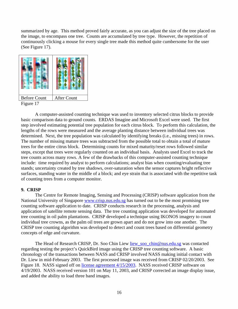
summarized by age. This method proved fairly accurate, as you can adjust the size of the tree placed on the image, to encompass one tree. Counts are accumulated by tree type. However, the repetition of continuously clicking a mouse for every single tree made this method quite cumbersome for the user (See Figure 17).

Before Count After Count Figure 17

A computer-assisted counting technique was used to inventory selected citrus blocks to provide

basic comparison data to ground counts. ERDAS Imagine and Microsoft Excel were used. The first step involved estimating potential tree population for each citrus block. To perform this calculation, the lengths of the rows were measured and the average planting distance between individual trees was determined. Next, the tree population was calculated by identifying breaks (i.e., missing trees) in rows. The number of missing mature trees was subtracted from the possible total to obtain a total of mature trees for the entire citrus block. Determining counts for mixed maturity/reset rows followed similar steps, except that trees were regularly counted on an individual basis. Analysts used Excel to track the tree counts across many rows. A few of the drawbacks of this computer-assisted counting technique include: time required by analyst to perform calculations; analyst bias when counting/evaluating tree stands; uncertainty created by tree shadows, over-saturation when the sensor captures bright reflective surfaces, standing water in the middle of a block; and eye strain that is associated with the repetitive task of counting trees from a computer monitor. 9. CRISP

The Centre for Remote Imaging, Sensing and Processing (CRISP) software application from the National University of Singapore www.crisp.nus.edu.sg has turned out to be the most promising tree counting software application to date. CRISP conducts research in the processing, analysis and application of satellite remote sensing data. The tree counting application was developed for automated tree counting in oil palm plantations. CRISP developed a technique using IKONOS imagery to count individual tree crowns, as the palm oil trees are grown apart and do not grow into one another. The CRISP tree counting algorithm was developed to detect and count trees based on differential geometry concepts of edge and curvature.

The Head of Research CRISP, Dr. Soo Chin Liew liew_soo_chin@nus.edu.sg was contacted

regarding testing the project’s QuickBird image using the CRISP tree counting software. A basic chronology of the transactions between NASS and CRISP involved NASS making initial contact with Dr. Liew in mid-February 2003. The first processed image was received from CRISP 02/20/2003. See Figure 18. NASS signed off on license agreement 4/15/2003. NASS received CRISP software on 4/19/2003. NASS received version 101 on May 11, 2003, and CRISP corrected an image display issue, and added the ability to load three band images.

17

An email response received from Dr.

Liew 02/20/2003 upon processing the citrus blocks stated, “We tested them out on our tree detecting software. The results are encouraging. We did not do much tweaking, just changed the window size of the filters. Our software expects to see trees brighter than the background, but your citrus trees are dark. So

we just inverted the brightness of the images before input to our software. It works pretty well, even for the mature trees, though there are still some undetected trees. A few large trees are counted twice. I think these minor problems can be overcome. I attach here the results of tree detection. The borders of each image have been excluded due to the nature of the windowing algorithm we use.” (Liew, 2003)

Image Enhancement

Before citrus tree counting could begin, much effort was made to determine which image enhancement modeling function would provide the highest degree of accuracy when used in conjunction with the CRISP software. Image enhancement is a processing procedure used to alter an image for ease of interpretation (NASA, 2003; Faust 1989). Types of image enhancement include spatial, radiometric and spectral enhancements. Spatial enhancement or filtering modifies the digital number (DN) values of pixels in an image, relative to the pixels that surround them was preferred for this investigation (ERDAS, 1999). Spatial enhancement examines the distribution of pixels of varying digital number (DN) value or “spatial frequency” over an image. The spatial frequency is defined as “the number of changes in brightness value per unit for any particular part of an image.” (Jensen, 1996; NASA, 2003)

ERDAS Imagine was used to import the images and begin preliminary processing. The resolution merge function using the principal components transform was performed on the QuickBird data to sharpen the spatial resolution of the imagery. This function fuses the PAN (0.61) meter with the multi-spectral (2.44) meter data to produce a multi-spectral four band image with a 0.61 meter ground resolution. Each raw panchromatic image is approximately 60 megabytes in size, while the four band multi-spectal image is 260 megabytes in size. The output from the resolution merge, created images nearly four gigabytes in size or larger.

Convolution filtering is a mathematical procedure for implementing spatial enhancement filters. With a convolution filter, pixel DN values are averaged over a square area, typically 3 x 3, 5 x 5 or 9 x 9, and all pixels values are replaced by this average DN value (NASA, 1999). Initial testing included fourteen convolution and six alternate filters using 3 x 3 and 5 x 5 kernels. Filters that provided the best results were retested. These filters included Edge Detect, Edge Enhance, High Pass, Haze Reduction, Laplacian, Summary, Prewitt, Sobel, Adaptive and Crisp. The High Pass Filter using a 3 x 3 kernel provided the best results in our study. This filter that passes or “emphasizes” high frequencies is an excellent tool for accentuating small details and edges (NASA, 1999). CRISP Program Evaluation

The CRISP software is currently being evaluated by NASS under a three month trial license. The agreement calls for NASS to provide the CRISP group with effective feedback on results and

Figure 18

18

performance, while abiding by their strict software license requirements. CRISP in return would attempt to work with NASS to enhance the software if possible and to meet the needs of NASS, and our customer, the Florida Department of Citrus. The CRISP User Manual states that CRISP uses intensity gradients to locate tree crowns. “It makes use of the concept of curvature in differential geometry to detect the edge pixels of each tree crown, and forms a model of intensity profile for each crown.” (Center for Remote Imagine, Sensing and Processing, 2003)

The CRISP software package offers the most promising software applications for separating and

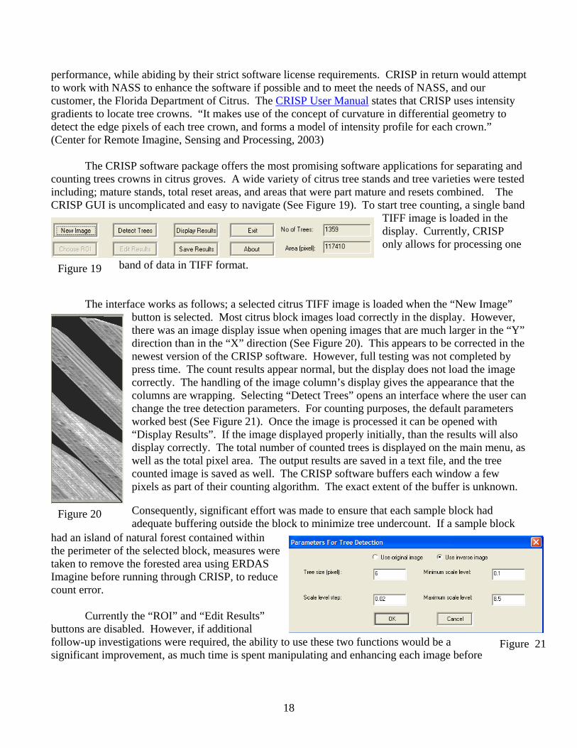
counting trees crowns in citrus groves. A wide variety of citrus tree stands and tree varieties were tested including; mature stands, total reset areas, and areas that were part mature and resets combined. The CRISP GUI is uncomplicated and easy to navigate (See Figure 19). To start tree counting, a single band

TIFF image is loaded in the display. Currently, CRISP only allows for processing one

band of data in TIFF format.

The interface works as follows; a selected citrus TIFF image is loaded when the “New Image”

button is selected. Most citrus block images load correctly in the display. However, there was an image display issue when opening images that are much larger in the “Y” direction than in the “X” direction (See Figure 20). This appears to be corrected in the newest version of the CRISP software. However, full testing was not completed by press time. The count results appear normal, but the display does not load the image correctly. The handling of the image column’s display gives the appearance that the columns are wrapping. Selecting “Detect Trees” opens an interface where the user can change the tree detection parameters. For counting purposes, the default parameters worked best (See Figure 21). Once the image is processed it can be opened with “Display Results”. If the image displayed properly initially, than the results will also display correctly. The total number of counted trees is displayed on the main menu, as well as the total pixel area. The output results are saved in a text file, and the tree counted image is saved as well. The CRISP software buffers each window a few pixels as part of their counting algorithm. The exact extent of the buffer is unknown.

Consequently, significant effort was made to ensure that each sample block had adequate buffering outside the block to minimize tree undercount. If a sample block

had an island of natural forest contained within the perimeter of the selected block, measures were taken to remove the forested area using ERDAS Imagine before running through CRISP, to reduce count error.

Currently the “ROI” and “Edit Results” buttons are disabled. However, if additional follow-up investigations were required, the ability to use these two functions would be a significant improvement, as much time is spent manipulating and enhancing each image before

Figure 20

Figure 19

Figure 21

19

processing through CRISP. Additionally, the ability to edit the output interactively could result in a reduction in error rates. CRISP Image Analysis

A detailed count analysis for all of the testing sites can be found in Appendix A where the

official tree counts are compared to the automated methods using various image bands and extraction techniques. Test sites one through three and thirty-two through thirty-nine were used as a basis to determine what image bands and enhancement techniques would provide the best counting results. Band one (visible blue) was chosen as the optimum band to use with CRISP, as the automated extraction was driven mainly by tree shadows, and perhaps the blue channel offers the best contrast between canopy/bare ground/shadow or penetration between them. For analysis purposes every test site was counted using the computer assisted count where possible, and for CRISP the raw image band one (blue), edge detection and high-pass filter were used.

The first three test sites were used for extensive testing of the CRISP software. See Appendix B

for the ground truth photos of the citrus block, panchromatic, multispectral, and CRISP images of the test sites. Test site 1 is a mature block characterized by very dense enclosed canopy resets generally planted where trees have been pushed. For all test sites, individual bands were stripped out from the main “resolution merged” image and run through CRISP separately. The visible blue, green, red, near IR and panchromatic bands were tested. Results derived from the processing of the single band data were evaluated. The best single band data were subsequently used to determine the best spatial enhancement (convolution) filters. Test site 2 is a part mature block mixed in with young trees and many young resets. The majority of convolution testing was performed on this site because of its diverse population, and to determine which band performed the best. Twenty-six different filters were run through this block, with the blue band performing the best in most cases. Test site 3 is characterized by a majority of resets and young trees with three full rows of mature trees. To complete the evaluation, the visible blue band was selected because it demonstrated the highest degree of accuracy, and three filters were chosen to run against it. The high pass spatial enhancement filter demonstrated the highest degree of accuracy followed closely by the edge detection filter and the unprocessed individual blue band of data with no enhancements. As expected the un-enhanced blue band performed the lowest compared to the enhanced images, while edge detection tended to fit in the middle of the pack, and the high pass filter was the best filter for determining tree counts.

The two other test sites were visited because of their unique physical orientation. Most of the

groves in our previous tests were characterized by a north/south orientation. Test site 4 is characterized by diagonal tree planting from true north. The rows run in a southeasterly to northwesterly direction. The rows in test site 5 run in an east to west direction. The orientation of these sites offered analysts the opportunity to examine the tree shadow complications that arise when imagery is acquired in the late Fall.

The raw image band and CRISP results for test site one, are displayed in Figures 22-24. The

individual bands are picking up unique tree properties, and CRISP is using the unique band properties to detect tree edges, and the results vary across all bands. For this example, bands 1 through 3 or Blue, Green, Red and the panchromatic band perform nearly identical with an 11 to 12 percent error rate. While band 4 or Near IR performs at near 18 percent error, which was an unexpected find, given the

20

belief that the Near IR band was assumed to be the best. An edge enhancement was performed on channel 2 or Green band, and the results performed as expected, where CRISP was able to determine the tree edges more efficiently, and reduced the error rate to 6 percent.

21

Figure 22 - Test site 1 Raw bands 1 & 2 with CRISP Results

Two images on left: Band 1 (blue) & CRISP Count 1309 Two images on right Band 2 (green) & CRISP Count 1324

Figure 23 Bands 3 & 4 with CRISP Results

Two images on left: Band 3 (red) & CRISP Count 1307 Two images on right: Band 4 (near ir) & CRISP Count 1227

Figure 24 Bands 5 & 2 with CRISP Results

Two images on left: Panchromatic & CRISP Count 1290 Two images on right: Band 2 Edge Enhanced & CRISP Count 1398 FASS Count 1495

22

The CRISP system places an oversized red pixel where the software determines that a tree centroid resides (See Figure 25). CRISP is able to accurately count the total number of trees in most areas to within 10-20 percent. The tree shadows appear to drive the placement of the tree centers, as CRISP looks for low pixel values to indicate the center of the tree’s canopy. Throughout the image, tree shadows have the lowest pixel value, while citrus trees have pixel values a little bit greater than shadows, and CRISP is placing tree centers where the shadows lie. Considering when the images were

observed; very late fall and sun angles are at their highest, it is amazing is that the tree counts are within an acceptable tolerance. Some of the trees are actually getting counted twice, but additional programs filter, or interactive editing could remove unacceptable tree placements. If the output results lying within rows are a little jagged, but the results accurate, where a tree center pixel is placed either at the center of a tree or the center of its shadow, then the software analysis is correctly performing its job.

Figure 25 Figure 26 is an enlargement of Test Site 1, an almost complete mature citrus block with only a handful of resets. The image on the left is a composite image of raw bands 1, 2, 3 or red, green, blue. The image in the middle was processed with ERDAS Imagine’s “3x3 high pass” filter, it is a single band unsigned 8 bit image. The “high pass” filter was then run through CRISP. The image on the right is the output from CRISP processing. CRISP computed 1,470 trees, while the grower reported 1498, a less than two percent difference. However, accuracies this close were not frequently observed. The CRISP output appears somewhat irregular in relation to the rows. In fact, it appears that the tree shadows are driving the tree count. And that is exactly what the CRISP algorithm looks for, the lowest pixel value in a given area. There does appear to be some double counting of trees, but most trees are getting counted in either the tree shadow or somewhere on the tree itself. There are some trees that are being placed outside the expected tree area or in the “buffer area”. However, the scene buffering in distance is unclear as of press time.

23

Figure 26 Enlargement of Test Site 1

QuickBird Bands 1,2,3 Bands 1,2,3 High Pass Filter CRISP Output

CRISP With Shadow Removal

Since CRISP seems to be counting a combination of trees and/or their shadows, a test was conducted to determine if CRISP could count citrus trees if all tree shadows from a selected block were removed. CRISP operates under the assumption that the citrus tree is the lowest pixel value in the scene. An unsupervised classification was run using ArcView GIS’s Image Analyst and 25 categories were chosen as output. The 25 categories were examined for shadows and the “shadow” categories were reassigned to category 255, effectively removing them from contaminating the tree count, and all other categories were set to 0, therefore making it a null pixel value. The original raw image was then mosaicked with the reassigned categorized image, where shadows in the original image were changed to 255, and the remaining values were not changed, because the mosaic process will not overlay a null pixel value over a valid one. The Citrus trees now had the lowest pixel values, and the shadows had a pixel value of 255. The mosaicked image was titled “shadow merged”. Figure 27 illustrates the CRISP

24

output derived from the “shadow merged” image without enhancements. The number of trees detect was 808 with this method. Figure 28 is the “shadow merged” image processed through the high pass filter, the results increased to 976 total trees. Figure 29 is the original raw image, processed through CRISP without enhancements, 1174 trees were counted. Figure 30 is the original image with a high pass filter run against it, 1304 trees were counted, and Figure 31 is the original resolution merge raw image. The FASS official number is 1497. The “shadow merge” image did not perform as well as expected, even when running through the high pass filter. A twenty six percent drop in accuracy occurred when comparing the normal high pass filter to the “shadow merge” filter, and a thirty six percent drop from the official FASS number.

Figure 27 Figure 28 Figure 29 Figure 30 Figure 31 CRISP Statistical Analysis

Two separate tree counting methods were tested; computer-assisted and CRISP. Initially all bands were tested on selected sample sites using CRISP to determine which band was optimum for tree counting. The blue band provided the best results for automated edge detection using CRISP. The sites were broken into three major categories based on the majority tree composition in a block. The categories were “Mature”, where the majority of tree rows had closed canopies, “Mixed Mature/Reset, where the majority could be either Mature or Resets, and “Reset” where most of the trees are resets, but there could be mature trees somewhere in the block.

The 53 testing sites were all run through CRISP’s software using the raw band 1 (visible blue)

“Raw_1”, edge detection enhancement (band 1) “EdgeD_1”, and high pass filter (band 1) “HighP_1” on

25

the original CRISP version, and the high pass filter “V2_HighP” on the newest CRISP version. The four automated tree detection methods were evaluated against the 53 sites, but the computer-assisted method was only evaluated with only 33. Two analyses were performed, one based on all 53 observations and another based only on those observations with comparable computer-assisted values. The computer-assisted technique was the most accurate of all measures, performing with a -1.25% average bias. The original CRISP high pass filter performed best (a measured average bias of approximately –14%) for the automated tree detection methods, with the newest CRISP high pass filter coming in second (-17% average bias). The newest CRISP version allows for three image bands, but the bands are averaged before computing the tree count, and that could account for the 3 percentage point drop. The edge detection filter provided the third most accurate results (-19% average bias), and the raw un-enhanced data performed the poorest (-24% average bias). As a footnote, surprisingly band 4 (Near IR) performed with the lowest accuracies of all bands, (i.e., 1, 2, 3, Pan). Table 2 shows bias, absolute deviation, and error measurement results comparing the four automated methods to the FASS values that are considered to be 'truth'. The best Bias (method - truth) performance among the automated methods is seen to be from the HighP_1 measure, followed closely by the V2_HighP value. The HighP_1 method is the 'best' considering all the measures available. It is interesting to note that all of the Bias estimates are negative, meaning that the automated methods consistently underestimate the tree count. Most of the total (Mean Squared Error, MSE) error between each methods measure and the actual count comes from sampling variation (Relative Variance), not from bias (MSE - Relative Variance).

Table 3 shows bias, absolute deviation, and error measurement results comparing the computer-assisted method and the four automated methods to the FASS values as 'truth'. These calculations are based only on the 33 comparable observations where all sites have all measures. In this analysis, the computer-assisted measure is clearly the best possible alternative, with the HighP_1 measure leading all the automated methods. Although the Bias estimate for computer-assisted is negative, it is sufficiently close to zero (approximately 1 percent) that you could not say it was over- or under-estimating the true value. The Relative MSE as a measure of total error is just under 10 percent.

26

However, the computer-assisted technique should not be relied upon as the best method, because it requires subjective decision making skills and requires significant analyst labor inputs. A regression analysis approach shows some promise for combining the computer-assisted approach with an automated method (such as HighP_1) to use the strengths of both approaches. The computer-assisted value would replace the FASS number as the dependent (Y) variable in a regression, while the automated method value would be the independent (X) variable in a regression estimation approach. Table 4 shows some preliminary data for regression analysis, using the FASS number as the (Y) variable since the computer-assisted value is not available in all observations. Data for both the entire set of observations and the subsets containing computer-assisted are shown. Figure 32 shows the HighP_1 regression versus FASS data based on 53 sites. Figure 33 shows the computer-assisted regression versus FASS data on 33 sites, and Figure 34 shows the comparable HighP_1 regression on 33 sites.

There were three sample sites deleted; one because a computer-assisted tree count was not visually possible because of ground noise, while the other two sites were not included because FASS recorded the sites as pushed while CRISP counted significant numbers of trees. The pushed blocks were not revisited due to the time constraints of press time.

27

Figure 32 Figure 33

Figure 34

CRISP Software Recommendations The following are some recommendations for CRISP software enhancements:

• Load file name currently processing in active window display • Fix display error when loading small area blocks for processing, error appears on column

wrapping o Fixed, but not fully evaluated

• Allow for dynamic region or area of interest selection (ROI) o Allow saving of ROI to disc o Not for trial version

• Allow for multi-band image analysis, currently only one band can be processed at a time o Newest CRISP version allows for three bands, but they are averaged

• Provide mechanism to dynamically edit processed trees to delete or add trees o Not for trail version

• Allow greater bit depth, currently 8-bit is the max, QuickBird is native 11 bit

28

• Create a filtering routine to examine tree placement just before the final results are displayed, to ensure that a tree does not get double counted and placed

Conclusion

The CRISP software proved to be a valuable tool for automating the counting of citrus trees. CRISP offers a unique opportunity to leverage the CRISP staff’s development experience in the palm oil counting field and apply their knowledge and techniques to solve many of the issues facing citrus tree counting. Although the computer-assisted method is the most accurate, it can be used to verify sampled CRISP counts in a certain area. High pass filtering was determined to be the best spatial enhancement; improving tree counts to within a –14 % average downward bias. However, more research is necessary to improve CRISP’s ability to separate tree canopies and improve the final tree counts for citrus.

If the program is to be expanded into large growing regions, it is recommended that a multi-resolution approach be used. First, using moderate resolution Landsat to identify the major citrus areas and estimate acreage, followed by targeted sampling using QuickBird data. The sampling could focus on areas where change detection from moderate resolution sensors determined that a significant event occurred, and QuickBird targeted on those sites could tell the extent of change. The sites could then be estimated using applications like CRISP to determine tree counts, using statistical analysis to support the findings.

From the authors perspective, this small scale pilot project was a good starting point and

provided considerable insight into the complexities and potential for citrus tree counting via QuickBird, in an area where ground counts were available to compare to. The information provided to the FDOC was substantial for a relatively small investment of resources. Acknowledgments The authors would like to thank the Florida Agricultural Statistics Service for their assistance and insight on this project. We want to especially recognize the Florida State Statistican John Witzig, along with Bob Terry, Harry Whittaker, Paul Messenger and Carol Armstrong. Their efforts and contributions are truly appreciated.

The authors would like to acknowledge and thank the members of the CRISP group in Singapore, especially Dr. Soo Chin Liew, Annie Hui and Mr. Fusheng Shi for developing and supporting the tree counting application and allowing NASS use of the trial version of the CRISP tree counting software.

The authors thank the Foreign Agricultural Service for their continued support and assistance on this project, especially Production Estimates and Crop Assessment Division Director, Allen Vandergriff, and Brazilian Analyst Michael Shean.

Appendices Appendix A Chosen Sample Sites & Counts Appendix B Ground Truth Testsites 1 – 5

29

Appendix A Chosen Sample Sites and Counts Band 1 Blue %diff Band 2 Green %diff Band 3 Red %diff Band 4 Near IR %diff Pan Band %diff Testsite 1 FASS Count 1498 Comp Assist 1443 -1.87 Raw Channel 1310 -12.6 1343 -10.3 1330 -11.2 1226 -18.2 1297 -13.4 Edge Detection 1359 -9.3 1333 -11.0 1358 -9.3 1387 -7.4 1321 -11.8 Edge Enhanced 1394 -6.9 1398 -6.7 1366 -8.8 1293 -13.7 1325 -11.5 High Pass 1543 3.0 1484 -0.9 1421 -5.1 1482 -1.1 1561 4.2 Haze Reduction 1478 -1.3 1453 -3.0 1408 -6.0 1366 -8.8 1408 -6.0 Laplacian 1287 -14.1 1290 -13.9 1371 -8.5 1306 -12.8 1248 -16.7 Summary 1499 0.1 1511 0.9 1415 -5.5 1406 -6.1 1510 0.8 Tree Age Mature Testsite 2 FASS Count 1495 Comp Assist 1269 Raw Channel 985 -34.1 985 -34.1 988 -33.9 963 -35.6 963 -35.6 Image Convolution 3x3 Kernel Edge Detection 1078 -27.9 1043 -30.2 1051 -29.7 1053 -29.6 1010 -32.4 Edge Enhanced 1028 -31.2 1028 -31.2 1043 -30.2 1020 -31.8 1015 -32.1 Low Pass 864 -42.2 862 -42.3 841 -43.7 885 -40.8 832 -44.3 High Pass 1117 -25.3 1131 -24.3 1087 -27.3 1131 -24.3 1099 -26.5 Haze Reduction 1078 -27.9 1089 -27.2 1063 -28.9 1074 -28.2 1064 -28.8 Vertical 849 -43.2 829 -44.5 817 -45.4 735 -50.8 770 -48.5 Laplacian 1158 -22.5 1121 -25.0 1151 -23.0 1074 -28.2 1072 -28.3 Horizontal Edge Detection 777 -48.0 742 -50.4 744 -50.2 766 -48.8 710 -52.5 Summary 1107 -26.0 1112 -25.6 1080 -27.8 1097 -26.6 1111 -25.7 Right Diagonal Edge 885 -40.8 873 -41.6 857 -42.7 845 -43.5 864 -42.2 Cross Edge Detection 952 -36.3 885 -40.8 893 -40.3 894 -40.2 939 -37.2 Horizontal 975 -34.8 883 -40.9 911 -39.1 892 -40.3 836 -44.1 Vertical Edge Detection 827 -44.7 807 -46.0 837 -44.0 777 -48.0 823 -44.9 Left Diagonal Edge 851 -43.1 787 -47.4 747 -50.0 729 -51.2 770 -48.5 5x5 Kernel Edge Detection 1032 -31.0 1015 -32.1 1021 -31.7 1113 -25.6 1033 -30.9 Edge Enhanced 1077 -28.0 1094 -26.8 1052 -29.6 1020 -31.8 1070 -28.4 High Pass 1004 -32.8 965 -35.5 958 -35.9 1067 -28.6 1024 -31.5 Haze Reduction 1124 -24.8 1089 -27.2 1077 -28.0 1081 -27.7 1076 -28.0 Summary 1069 -28.5 1112 -25.6 1045 -30.1 1058 -29.2 1036 -30.7

30

Other Filters Non-Directional Edge Pre 1061 -29.0 1050 -29.8 1007 -32.6 1020 -31.8 1052 -29.6 Non-Directional Edge Sob 1054 -29.5 1053 -29.6 1023 -31.6 1038 -30.6 1017 -32.0 Statistical Filter 765 -48.8 774 -48.2 880 -41.1 1036 -30.7 705 -52.8 Crisp 1053 -29.6 1059 -29.2 1079 -27.8 1036 -30.7 1029 -31.2 Focal Analysis 838 -43.9 849 -43.2 847 -43.3 869 -41.9 846 -43.4 Wallis Adaptive Filter (3x3) 1077 -28.0 1094 -26.8 1043 -30.2 1020 -31.8 1015 -32.1 Wallis Adaptive Filter (5x5) 1028 -31.2 1051 -29.7 1052 -29.6 1083 -27.6 1070 -28.4 Tree Age Mature/Reset Testsite 3 FASS Count 1498.0 Comp Assist 863.0 Raw Channel 1073 -28.4 1072 -28.4 1039 -30.6 936 -37.5 1028 -31.4 Edge Detection 1164 -22.3 1180 -21.2 1167 -22.1 1166 -22.2 1150 -23.2 Edge Enhanced 1163 -22.4 1156 -22.8 1114 -25.6 1039 -30.6 1118 -25.4 High Pass 1318 -12.0 1268 -15.4 1216 -18.8 1245 -16.9 1276 -14.8 Haze Reduction 1218 -18.7 1219 -18.6 1194 -20.3 1130 -24.6 1181 -21.2 Laplacian 1206 -19.5 1195 -20.2 1203 -19.7 1187 -20.8 1134 -24.3 Summary 1268 -15.4 1272 -15.1 1232 -17.8 1165 -22.2 1214 -19.0 Tree Age Reset Testsite 4 %diff Raw Channel 1 1142 -23.7 Channel 1 Edge Detection 1109 -25.9 Channel 1 High Pass 1283 -14.2 FASS Count 1496 Computer Assisted Count 1475 -1.4 Tree Age Mature Testsite 5 Raw Channel 1 1142 -22.9 Channel 1 Edge Detection 1231 -16.9 Channel 1 High Pass 1255 -15.3 FASS Count 1482 Computer Assisted Count 1560 5.3 Tree Age Mature Testsite 6 Raw Channel 1 1122 -25.0 Channel 1 Edge Detection 1105 -26.1 Channel 1 High Pass 1275 -14.8 FASS Count 1496 Computer Assisted Count 1609 7.6 Tree Age Mature

31

Testsite 7 Raw Channel 1 1092 -27.0 Channel 1 Edge Detection 1095 -26.8 Channel 1 High Pass 1160 -22.5 FASS Count 1496 Computer Assisted Count 1526 2.0 Tree Age Mature Testsite 8 Raw Channel 1 1186 -20.7 Channel 1 Edge Detection 1164 -22.2 Channel 1 High Pass 1282 -14.3 FASS Count 1496 Computer Assisted Count 1424 -4.8 Tree Age Mature Testsite 9 Raw Channel 1 1138 -20.3 Channel 1 Edge Detection 973 -31.9 Channel 1 High Pass 1271 -11.0 FASS Count 1428 Computer Assisted Count 1363 -4.6 Tree Age Mature Testsite 10 Raw Channel 1 1160 -22.5 Channel 1 Edge Detection 1176 -21.4 Channel 1 High Pass 1241 -17.1 FASS Count 1497 Computer Assisted Count 1487 -0.7 Tree Age Mature Testsite 11 Raw Channel 1 1122 -25.1 Channel 1 Edge Detection 1177 -21.4 Channel 1 High Pass 1255 -16.2 FASS Count 1498 Computer Assisted Count 1446 -3.5 Tree Age Mature/Reset Testsite 12 Raw Channel 1 1087 -32.0 Channel 1 Edge Detection 997 -37.6

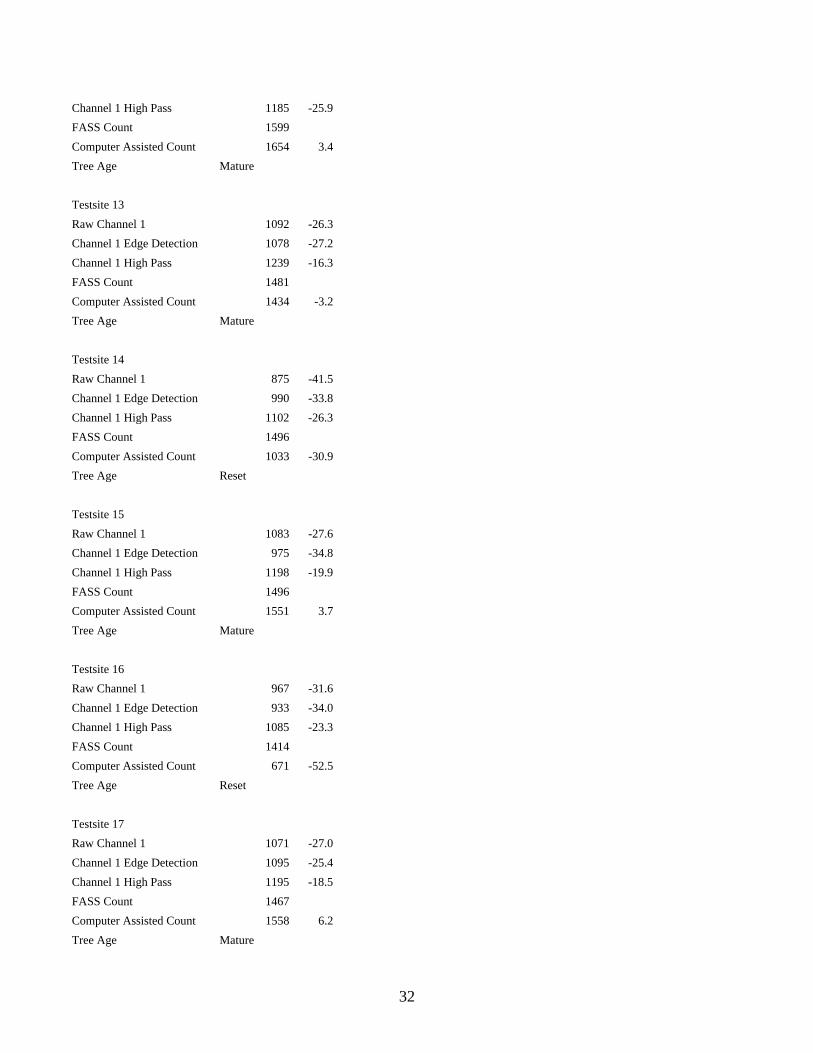
32

Channel 1 High Pass 1185 -25.9 FASS Count 1599 Computer Assisted Count 1654 3.4 Tree Age Mature Testsite 13 Raw Channel 1 1092 -26.3 Channel 1 Edge Detection 1078 -27.2 Channel 1 High Pass 1239 -16.3 FASS Count 1481 Computer Assisted Count 1434 -3.2 Tree Age Mature Testsite 14 Raw Channel 1 875 -41.5 Channel 1 Edge Detection 990 -33.8 Channel 1 High Pass 1102 -26.3 FASS Count 1496 Computer Assisted Count 1033 -30.9 Tree Age Reset Testsite 15 Raw Channel 1 1083 -27.6 Channel 1 Edge Detection 975 -34.8 Channel 1 High Pass 1198 -19.9 FASS Count 1496 Computer Assisted Count 1551 3.7 Tree Age Mature Testsite 16 Raw Channel 1 967 -31.6 Channel 1 Edge Detection 933 -34.0 Channel 1 High Pass 1085 -23.3 FASS Count 1414 Computer Assisted Count 671 -52.5 Tree Age Reset Testsite 17 Raw Channel 1 1071 -27.0 Channel 1 Edge Detection 1095 -25.4 Channel 1 High Pass 1195 -18.5 FASS Count 1467 Computer Assisted Count 1558 6.2 Tree Age Mature

33

Testsite 18 Raw Channel 1 1107 -26.1 Channel 1 Edge Detection 1099 -26.6 Channel 1 High Pass 1223 -18.3 FASS Count 1497 Computer Assisted Count 1400 -6.5 Tree Age Mature Testsite 19 Raw Channel 1 916 -35.7 Channel 1 Edge Detection 962 -32.4 Channel 1 High Pass 1024 -28.1 FASS Count 1424 Computer Assisted Count 1398 -1.8 Tree Age Mature Testsite 20 Raw Channel 1 874 -24.3 Channel 1 Edge Detection 877 -24.1 Channel 1 High Pass 980 -15.2 FASS Count 1155 Computer Assisted Count 1189 2.9 Tree Age Mature Testsite 21 Raw Channel 1 1181 -20.3 Channel 1 Edge Detection 1130 -23.7 Channel 1 High Pass 1307 -11.7 FASS Count 1481 Computer Assisted Count 1415 -4.5 Tree Age Reset Testsite 22 Raw Channel 1 825 -37.8 Channel 1 Edge Detection 730 -45.0 Channel 1 High Pass 914 -31.1 FASS Count 1327 Computer Assisted Count 1340 1.0 Tree Age Mature Testsite 23 Raw Channel 1 1174 -21.6 Channel 1 Edge Detection 1157 -22.7

34

Channel 1 High Pass 1304 -12.9 FASS Count 1497 Computer Assisted Count 1634 9.2 Tree Age Mature Testsite 24 Raw Channel 1 1039 -30.5 Channel 1 Edge Detection 1009 -32.6 Channel 1 High Pass 1247 -16.6 FASS Count 1496 Computer Assisted Count 1634 9.2 Tree Age Mature Testsite 25 Raw Channel 1 1046 -41.8 Channel 1 Edge Detection 1033 -42.5 Channel 1 High Pass 1240 -31.0 FASS Count 1798 Computer Assisted Count 1694 -5.8 Tree Age Mature Testsite 26 Raw Channel 1 1211 -18.2 Channel 1 Edge Detection 1219 -17.7 Channel 1 High Pass 1365 -7.8 FASS Count 1481 Computer Assisted Count 1567 5.8 Tree Age Mature testsite null Dropped from analysis dataset, trees visually undetectable Raw Channel 1 976 -34.8 Channel 1 Edge Detection 1090 -27.1 Channel 1 High Pass 1189 -20.5 FASS Count 1496 Computer Assisted Count 0 -100.0 Tree Age Reset Testsite 27 Raw Channel 1 1025 -24.4 Channel 1 Edge Detection 1017 -24.9 Channel 1 High Pass 1197 -11.7 FASS Count 1355 Computer Assisted Count 1352 -0.2 Tree Age Mature

35

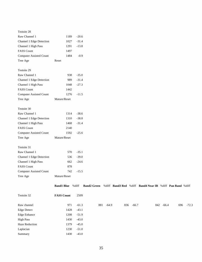
Testsite 28 Raw Channel 1 1189 -20.6 Channel 1 Edge Detection 1027 -31.4 Channel 1 High Pass 1291 -13.8 FASS Count 1497 Computer Assisted Count 1484 -0.9 Tree Age Reset Testsite 29 Raw Channel 1 938 -35.0 Channel 1 Edge Detection 989 -31.4 Channel 1 High Pass 1048 -27.3 FASS Count 1442 Computer Assisted Count 1276 -11.5 Tree Age Mature/Reset Testsite 30 Raw Channel 1 1314 -38.6 Channel 1 Edge Detection 1310 -38.8 Channel 1 High Pass 1468 -31.4 FASS Count 2140 Computer Assisted Count 1592 -25.6 Tree Age Mature/Reset Testsite 31 Raw Channel 1 570 -35.1 Channel 1 Edge Detection 536 -39.0 Channel 1 High Pass 662 -24.6 FASS Count 878 Computer Assisted Count 742 -15.5 Tree Age Mature/Reset Band1 Blue %diff Band2 Green %diff Band3 Red %diff Band4 Near IR %diff Pan Band %diff Testsite 32 FASS Count 2509 Raw channel 971 -61.3 881 -64.9 836 -66.7 842 -66.4 696 -72.3 Edge Detect 1428 -43.1 Edge Enhance 1208 -51.9 High Pass 1430 -43.0 Haze Reduction 1379 -45.0 Laplacian 1230 -51.0 Summary 1430 -43.0

36

Non-Directional Edge Pre 1333 -46.9 Non-Directional Edge Sob 1338 -46.7 Wallis Adaptive Filter 1208 -51.9 Crisp 1276 -49.1 Tree Age Mature Testsite 33 FASS Count 12260 Raw channel 11263 -8.1 11121 -9.3 11130 -9.2 10759 -12.2 10918 -10.9 Edge Detect 12760 4.1 Edge Enhance 11581 -5.5 High Pass 12179 -0.7 Haze Reduction 11938 -2.6 Laplacian 13299 8.5 Summary 12066 -1.6 Non-Directional Edge Pre 12379 1.0 Non-Directional Edge Sob 12499 1.9 Wallis Adaptive Filter 11581 -5.5 Crisp 11746 -4.2 Tree Age Mature Testsite 34 FASS Count 5923 Raw channel 2423 -59.1 2381 -59.8 2388 -59.7 2188 -63.1 2284 -61.4 Edge Detect 2833 -52.2 Edge Enhance 2504 -57.7 High Pass 2713 -54.2 Haze Reduction 2609 -56.0 Laplacian 2849 -51.9 Summary 2639 -55.4 Non-Directional Edge Pre 2571 -56.6 Non-Directional Edge Sob 2573 -56.6 Wallis Adaptive Filter 2504 -57.7 Crisp 2557 -56.8 Tree Age Mature Testsite 35 FASS Count 13429 Raw channel 8307 -38.1 8226 -38.7 8274 -38.4 7682 -42.8 7976 -40.6 Edge Detect 9649 -28.1 Edge Enhance 8550 -36.3 High Pass 9057 -32.6 Haze Reduction 8765 -34.7 Laplacian 9612 -28.4

37

Summary 8913 -33.6 Non-Directional Edge Pre 9228 -31.3 Non-Directional Edge Sob 9203 -31.5 Wallis Adaptive Filter 8550 -36.3 Crisp 8615 -35.8 Tree Age Mature Testsite 36 FASS Count 3564 Raw channel 4275 19.9 4234 18.8 4213 18.2 3928 10.2 4042 13.4 Edge Detect 4670 31.0 4316 21.1 Edge Enhance 4381 22.9 4110 15.3 High Pass 4636 30.1 4443 24.7 Haze Reduction 4518 26.8 4252 19.3 Laplacian 4515 26.7 4403 23.5 Summary 4574 28.3 4326 21.4 Non-Directional Edge Pre 4337 21.7 4292 20.4 Non-Directional Edge Sob 4336 21.7 4336 21.7 Wallis Adaptive Filter 4361 22.4 4110 15.3 Crisp 4417 23.9 4152 16.5 Tree Age Mature Testsite 37 Band1 Blue %diff Band2 Green %diff Band3 Red %diff Band4 Near IR %diff Pan Band %diff FASS Count 2903 Raw channel 2180 -24.9 2094 -27.9 2152 -25.9 1767 -39.1 1892 -34.8 Edge Detect 2388 -17.8 Edge Enhance 2321 -20.1 High Pass 2592 -10.7 Haze Reduction 2447 -15.7 Laplacian 2375 -18.2 Summary 2521 -13.2 Non-Directional Edge Pre 2127 -26.8 Non-Directional Edge Sob 2167 -25.4 Wallis Adaptive Filter 2321 -20.1 Crisp 2386 -17.8 Tree Age Mature Testsite 38 FASS Count 1323 Raw channel 1027 -22.4 971 -26.6 1022 -22.8 787 -40.5 838 -36.7 Edge Detect 1158 -12.5 Edge Enhance 1116 -15.6

38

High Pass 1217 -8.0 Haze Reduction 1173 -11.3 Laplacian 1133 -14.4 Summary 1191 -10.0 Non-Directional Edge Pre 1053 -20.4 Non-Directional Edge Sob 1054 -20.3 Wallis Adaptive Filter 1116 -15.6 Crisp 1138 -14.0 Tree Age Mature Testsite 39 FASS Count 4186 Raw channel 3776 -9.8 3716 -11.2 3752 -10.4 3582 -14.4 3646 -12.9 Edge Detect 4210 0.6 Edge Enhance 3897 -6.9 High Pass 4065 -2.9 Haze Reduction 3986 -4.8 Laplacian 4525 8.1 Summary 4051 -3.2 Non-Directional Edge Pre 4150 -0.9 Non-Directional Edge Sob 4115 -1.7 Wallis Adaptive Filter 3897 -6.9 Crisp 3943 -5.8 Tree Age Mature Not used in analysis FASS Count 0.0 Pushed Not used in analysis Raw channel 5502 N/A 5502 N/A 4921 N/A 4916 N/A 4491 N/A Edge Detect Edge Enhance High Pass Haze Reduction Laplacian Summary Non-Directional Edge Prewitt Filter Non-Directional Edge Sobel Filter Wallis Adaptive Filter Crisp Tree Age Reset Not used in analysis FASS Count 0.0 Pushed Not used in analysis Raw channel 2911 N.A 2690 N.A 2911 N.A 2920 N.A 2597 N/A Edge Detect 3757

39

Edge Enhance 3521 High Pass Haze Reduction Laplacian Summary Non-Directional Edge Prewitt Filter Non-Directional Edge Sobel Filter Wallis Adaptive Filter Crisp Tree Age Reset Testsite 40 %diff Raw Channel 1 1316 -51.7 Channel 1 Edge Detection 1318 -51.7 Channel 1 High Pass 1481 -45.7 FASS Count 2726 Tree Age Mature Testsite 41 Raw Channel 1 1288 -64.3 Channel 1 Edge Detection 1331 -63.1 Channel 1 High Pass 1496 -58.5 FASS Count 3606 Tree Age Mature Testsite 42 Raw Channel 1 4593 -8.5 Channel 1 Edge Detection 4695 -6.4 Channel 1 High Pass 5029 0.2 FASS Count 5017 Tree Age Mature Testsite 43 Raw Channel 1 7298 -9.5 Channel 1 Edge Detection 7735 -4.1 Channel 1 High Pass 8451 4.8 FASS Count 8066 Tree Age Mature Testsite 44 Raw Channel 1 3808 0.4 Channel 1 Edge Detection 4403 16.1 Channel 1 High Pass 4391 15.8 FASS Count 3792

40

Tree Age Mature Testsite 45 Raw Channel 1 3870 -1.6 Channel 1 Edge Detection 4373 11.2 Channel 1 High Pass 4335 10.2 FASS Count 3934 Tree Age Mature/Reset Testsite 46 Raw Channel 1 5725 5.5 Channel 1 Edge Detection 6703 23.6 Channel 1 High Pass 6651 22.6 FASS Count 5425 Tree Age Mature Testsite 47 Raw Channel 1 15492 -19.7 Channel 1 Edge Detection 16902 -12.4 Channel 1 High Pass 17277 -10.5 FASS Count 19294 Tree Age Mature/Reset Testsite 48 Raw Channel 1 5340 -16.8 Channel 1 Edge Detection 5923 -7.7 Channel 1 High Pass 6504 1.3 FASS Count 6419 Tree Age Reset Testsite 49 Raw Channel 1 13702 -12.7 Channel 1 Edge Detection 11,442 -27.1 Channel 1 High Pass 15891 1.2 FASS Count 15698 Tree Age Mature Testsite 50 Raw Channel 1 15438 -37.0 Channel 1 Edge Detection 17453 -28.8 Channel 1 High Pass 17518 -28.5 FASS Count 24516 Tree Age Mature

41

Testsite 51 Raw Channel 1 1624 -5.0 Channel 1 Edge Detection 1685 -1.5 Channel 1 High Pass 1755 2.6 FASS Count 1710 Tree Age Mature Testsite 52 Raw Channel 1 2878 -29.5 Channel 1 Edge Detection 3069 -24.8 Channel 1 High Pass 3333 -18.3 FASS Count 4082 Tree Age Reset Testsite 53 Raw Channel 1 556 48.7 Channel 1 Edge Detection 592 58.3 Channel 1 High Pass 619 65.5 Manual Count 702 -39.2 Berry Count 374 Tree Age Mature/Reset Testsite 54 Raw Channel 1 1155 -9.9 Channel 1 Edge Detection 1284 0.2 Channel 1 High Pass 1301 1.5 Manual Count 1289 0.5 Berry Count 1282 Tree Age Mature

42

Appendix B Photos, Raw, and Processed Images Testsite 1, Ground Truth 4/23/2003

Panchromatic Multispectral CRISP

43

Testsite 2, Ground Truth 4/23/2003

Panchromatic Multispectral CRISP

44

Testsite 3, Ground Truth 4/23/2003

Panchromatic Multispectral CRISP

45

Testsite 4, Ground Truth 4/23/2003

Panchromatic

Multispectral

CRISP

46

Testsite 5, Ground Truth 4/23/2003

Panchromatic

Multispectral

CRISP

47

Authors USDA/NASS/Research & Development Division

George Hanuschak, Director Rick Mueller, Remote Sensing Analyst Claire Boryan, Remote Sensing Analyst Mike Craig, Senior Remote Sensing Analyst

USDA/NASS/Information Technology Division Mike Fleming, Mathematical Statistician

References Craig, M.E. (2001) “A Resource Sharing Approach to Crop Identification and Estimation.” ASPRS

2001 Annual Convention Technical Papers, St. Louis, Missouri, April 2001. Center for Remote Imaging, Sensing and Processing (CRISP), Tree Counting Software (Trial Version 1)

User Manual, April 2003. Digital Globe, “Standard Imagery System Features and Benefits.” at http://www.digitalglobe.com/. 6 May 2003. ERDAS, 1999. ERDAS: Field Guide, Fifth Edition. Atlanta, Georgia. Faust, Nickolas L. 1989. “ Image Enhancement.” Volume 20, Supplement 5 of Encyclopedia of

Computer Science and Technology, edited by Allen Kent and James G. Williams. New York: Marcel Dekker, Inc.

Gordon, D.K., and W.R. Philipson. 1986. “A Texture-Enhancement Procedure for Separating Orchard

from Forest in Thematic Mapper Data.” International Journal of Remote Sensing, Vol. 7, No. 2: 301-304.

Gordon, D. K., et al. 1986. “Fruit Tree Inventory with Landsat Thematic Mapper Data.”

Photogrammetric Engineering and Remote Sensing, Vol. 52, No. 12:1871-1876. Hanuschak, G., and R. Mueller. 2002. "Cost and Benefit Analysis of a Cropland Data Layer", Pecora 15

Conference on 'Integrating Remote Sensing at the Global, Regional, and Local Scale', Denver, CO. Jensen, John R. 1996. Introductory Digital Image Processing: A Remote Sensing Perspective.

Englewood Cliffs, New Jersey: Prentice Hall. Kay, Simon et al., 2003. “Geometric Quality Assessment of Orthorectified VHR Space Image Data.”

Photogrammetric Engineering & Remote Sensing, Vol. 69, No. 5: 484-491. Liew, S.C. Re: Palm Oil Tree Counting. (3 March 2003).

48

Mueller, R. and Ozga, M. (2002) "Creating a Cropland Data Layer For an Entire State", Proceedings of the ACSM-ASPRS 2002 Conference, in Washington DC, ASPRS, Bethesda, MD, April 2002.

NASA. “ The Remote Sensing Tutorial: What You Can Learn From Sensors On Spacecraft that Look

Inward at the Earth and Outward at the Planets, The Galaxies and , Going Back in Time, The Cosmos.” at http://rst.gsfc.nasa.gov/AppD/glossary.html, 5 May 2003.

Taberner, M.J., et al. 1987. “Spectral and Spatial Characterisation of Orchards in New York State Using

Thematic Mapper Imagery.” Paper presented at the Twenty First International Symposium on Remote Sensing of the Environment, Ann Arbor, Michigan.

Toutin, T. 2003, “Geometric Processing of Remote Sensing Images: Models Algorithms, and Methods.” International Journal of Remote Sensing (in press).