pilot investigation of slowsand filtration and reverse ... · pilot investigation of slowsand...

Pilot Investigation of Slowsand Filtrationand Reverse Osmosis Treatment ofCentral Arizona Project Water

Advanced Water Treatment Research ProgramReport No. 90

U.S. Department of the InteriorBureau of Reclamation

August 2002

REPORT DOCUMENTATION PAGE Form ApprovedOMB No. 0704-0188

Public reporting burden for this collection of information is estimated to average 1 hour per response, including the time for reviewing instructions, searching existingdata sources, gathering and maintaining the data needed, and completing and reviewing the collection of information. Send comments regarding this burdenestimate or any other aspect of this collection of information, including suggestions for reducing this burden to Washington Headquarters Services, Directoratefor Information Operations and Reports, 1215 Jefferson Davis Highway, Suit 1204, Arlington VA 22202-4302, and to the Office of Management and Budget,Paperwork Reduction Report (0704-0188), Washington DC 20503.

1. AGENCY USE ONLY (Leave Blank) 2. REPORT DATE August 2002

3. REPORT TYPE AND DATES COVERED

4. TITLE AND SUBTITLE

Pilot Investigation of Slowsand Filtration and Reverse Osmosis Treatmentof Central Arizona Project Water

5. FUNDING NUMBERS

6. AUTHOR(S)

Charles Moody, Bruce Garrett, and Eric Holler7. PERFORMING ORGANIZATION NAME(S) AND ADDRESS(ES)

U.S. Department of the InteriorBureau of ReclamationPhoenix Area OfficePO Box 81169Phoenix AZ 85069-1169

8. PERFORMING ORGANIZATIONREPORT NUMBERAdvanced Water TreatmentResearch Program ReportNo. 90

9. SPONSORING/MONITORING AGENCY NAME(S) AND ADDRESS(ES)

Bureau of Reclamation Science & Technology Program, Denver, COCentral Arizona Water Conservation District, Phoenix, AZTown of Marana, Marana, AZFlowing Wells Irrigation District, Tucson, AZTown of Oro Valley, Tucson, AZMetropolitan Domestic Water Improvement District, Tucson, AZ

10. SPONSORING/MONITORINGAGENCY REPORT NUMBER

11. SUPPLEMENTARY NOTES

12a. DISTRIBUTION/AVAILABILITY STATEMENT

Available from the National Technical Information Service,Operations Division, 5285 Port Royal Road, Springfield, Virginia 22161

12b. DISTRIBUTION CODE

13. ABSTRACT (Maximum 200 words)

Because the August 2000 Bureau of Reclamation report, Alternatives for Using Central ArizonaProject Water in the Northwest Tucson Area, identified slowsand filtration (SSF) as the lowest costwater treatment alternative for a proposed 40-MGD water treatment plant, this pilot investigationevaluated the technical effectiveness of SSF treatment of Central Arizona Project (CAP) water. Based on low turbidity levels in the SSF-treated water, subject to obtaining successful operationduring the summer, the authors recommend SSF treatment. At a filtration rate of 0.11 gal/min/ft2

(0.27 m/h, 6.9 MGD/acre) the SSF filter run length measured 22 days. With 17 SSF cleanings peryear, the revised SSF treatment cost estimate is $0.16 per thousand gallons. For treatment withdesalting, based on low fouling of low-pressure reverse osmosis (RO) polyamide membraneequipment operating on SSF-treated CAP water, the authors recommend either of two treatmentcombinations: (1) microfiltration or ultrafiltration - RO or (2) SSF - RO.14. SUBJECT TERMS–

water treatment, desalting, Colorado River, pilot tests, slowsand filtration, reverseosmosis

15. NUMBER OFPAGES 60

16. PRICE CODE

17. SECURITY CLASSIFICATION OF REPORT UL

18. SECURITY CLASSIFICATIONOF THIS PAGE UL

19. SECURITY CLASSIFICATIONOF ABSTRACT UL

20. LIMITATION OFABSTRACT UL

NSN 7540-01-280-5500 Standard Form 298 (Rev. 2-89)Prescribed by ANSI Std. 239-18

298-102

Pilot Investigation of SlowsandFiltration and Reverse OsmosisTreatment of Central ArizonaProject Water

Advanced Water Treatment Research ProgramReport No. 90

byCharles MoodyBruce GarrettEric Holler

Department of the InteriorBureau of Reclamation

August 2002

Mission Statements

The mission of the Department of the Interior is to protect and provideaccess to our Nation’s natural and cultural heritage and honor our

trust responsibilities to tribes.

The mission of the Bureau of Reclamation is to manage, develop, andprotect water and related resources in an environmentally and economically

sound manner in the interest of the American Public.

Acknowledgments

The Bureau of Reclamation’s (Reclamation) Science and Technology Program, Reclamation’s Phoenix AreaOffice, and the water provider oganizations listed below contributed funds and services to conduct this study. Eric Holler (Reclamation) initiated and advocated the study and coordinated its implementation.

This report summarizes work undertaken by various agencies for the Southern Arizona Water ManagementStudy to study the effectiveness of slowsand filtration (SSF) and reverse osmosis treatment of Central ArizonaProject (CAP) water. The organizations and their participation follow:

Central Arizona Water Conservation District (CAWCD) – Hosted the pilot test at the Twin PeaksPumping Plant Complex. The CAWCD provided water, installed wiring and provided power duringoperation, provided the earthen pad on which the slowsand tank was placed, and provided sitesecurity.

Town of Marana – Demobilized the SSF tank from Tucson Water’s Hayden-Udall Treatment Plant andtransported the tank to the Twin Peaks site. Marana representatives set the tank in place, providedequipment (including a crane) and labor to place the gravel underdrain and the specialty sand,provided a water meter to measure inlet flows, and demobilized and removed the tank uponcompletion of the testing.

Flowing Wells Irrigation District – Provided professional installation of the plumbing and piping betweenthe SSF and the Mobile Treatment Plant, including overflows, drains, stands, supports, and SSFproduct water piping; and installed a float valve (at their suggestion) on the inlet to the SSF tank,which significantly improved operation.

Town of Oro Valley – Provided materials and installation of the inlet water piping, provided weeklysampling and water quality testing for the extensive monitoring that was required. Water qualitytesting included sampling at five locations for a large variety of constituents.

Metropolitan Domestic Water Improvement District (MDWID) – Provided comprehensive monthly waterquality sampling and testing using the same methodology as Oro Valley. Acted as a clearinghouse forOro Valley and MDWID to gather water quality information and input the data into the spreadsheet.

I thank the following individuals representing these water providers: Mark Stratton, Charlie Maish,Mike Block, and Stephanie Pranshke, MDWID; Bob Bradford, Dave Gunn, Mike Early, andTom Plasay, CAWCD; Brad DeSpain, Town of Marana; Alan Forrest, Mary Kobida, and Charlie Soper, Townof Oro Valley; David Crockett and Jim Cavanaugh, Flowing Wells Irrigation District; Joe Crowson, BradPrudhom, and Eric Holler, Reclamation. A special thank you is extended to Reclamation’s consultingchemical engineer, Bruce Garrett, P.E., who made the pilot operational, operated and maintained the pilot,provided water quality testing, participated in presentations, and prepared the extensive data documentationand data reduction contained in appendices B and C. Without Mr. Garrett’s expertise and dedication, thepilot would not have been possible.

It was a pleasure to work with this group of people. Their unflagging willingness to contribute to ourcommon goals made this investigation possible. Together, they have continued to illustrate the positiveimpact a collaborative effort can make.

And, finally, I thank the others on the team from Reclamation who put together technical information andcompiled and edited the report: Qian Zhang, water treatment; Sharon Leffel, editing and desktop publishing;Rodney Tang, technical support; Robert Michaels, management support; and Suzanne Sikora, financialmanagement.

Charles ”Chuck“ Moody, Ph.D., P.E., Project Manager

Acronyms and Abbreviations

A

ADEQ Arizona Department of Environmental QualityAFY acre-feet per year of water flow; multiply by 0.620 to convert to gallons

per minute; divide by 724 to convert to cubic feet per secondASR aquifer storage and recoveryAWWA American Water Works Association

C

°C degrees CelsiusCA cellulose acetateCAP Central Arizona ProjectCASI Central Arizona Salinity InterceptorCAWCD Central Arizona Water Conservation Districtcfs cubic feet per secondcfu colony forming unitsCO2 carbon dioxideCOU coefficient of uniformityCT conventional treatment (coagulation, flocculation, and rapid sand

filtration)CT - RO combination of conventional treatment and reverse osmosis

D

DBPs disinfection byproductsD/DBPR Disinfectant/Disinfection Byproducts RuleDO dissolved oxygendP difference in pressure between two locations

E

EPA Environmental Protection AgencyERT energy recovery turbine

F

ft foot; feetft2 square feet

G

gal/min gallons per minutegal/min/ft2 gallons per minute per square footgfd gallons of permeate per square foot of membrane per daygal/f2/day gallons per square foot per day membrane water fluxgpd gallons per daygpg grains per gallongpm gallons per minutegpm/ft2 gallons per minute per square foot

H

HAA haloacetic acidHAA5 group of five haloacetic acids regulated by the Safe Drinking Water Act

Stage 1 Disinfectants and Disinfection Products Rule with an MCL of 0.080 milligrams per liter

hp horsepowerHPC heterotrophic plate count

I

ICP inductively coupled plasma

K

kg kilogram(s)

L

LOI loss on ignitionL/m liters per minute

M

m meter(s)m2 square metersMBD mass balance deviation

MCL maximum contaminant levelMF microfiltrationMF/UF microfiltration or ultrafiltrationMF/UF - RO combination of microfiltration/ultrafiltration and reverse osmosisMGD million gallons per day; multiply by 1,121 to convert to acre-feet per yearmg/L milligrams per liter concentrationm/h meters per hourm3/h cubic meters per hourmm millimeter(s)MTP Mobile Water Treatment Plant�m micrometer(s)�g/L micrograms per liter

N

NTU nephelometric turbidity unit

O

O&M operation and maintenance

P

PA polyamidepH A measure of the relative acidity of water. pH depends on the

composition of salts (electrolytes) dissolved in the water. Acid waters have pH values less than 7. Basic waters have pH values greater than 7.

ppm parts per millionpsi pounds per square inch pressure; divide by 14.5 to convert to bars;

multiply by 6.895 to convert to kilopascalspsid psi differential pressurepsig psi gage pressure (add atmospheric pressure to get absolute pressure)

R

Reclamation Bureau of ReclamationRO reverse osmosisROSA Reverse Osmosis System Analysis (DOW computer program)

S

SARWMS Southern Arizona Regional Water Management StudySDI Silt Density Index

SDS simulated distribution systemSDSDBP simulated distribution system disinfection byproductSDSHAA simulated distribution system haloacetic acidSDSTHM simulated distribution system trihalomethaneSDWA Safe Drinking Water ActSSF slowsand filtrationSSF - RO combination of slowsand filtration and reverse osmosisSWTR Surface Water Treatment Rule

T

TDS total dissolved solids, milligrams per literTHM trihalomethaneTHMFP Trihalomethane Formation PotentialTOC total organic carbon, milligrams per literTTHM total trihalomethanest-value statistical students' t-value

U

UF ultrafiltration

V

VFD variable frequency drive

Contents

Page

S-1 Executive Summary

1 Introduction4 Education and Public Information5 Slowsand Filtration8 SSF Pilot Tests8 Test Site

10 Pilot Equipment13 Test Period14 Water Supply14 Operating Conditions15 Filtration Rates15 Filter Cleaning16 SSF Results16 Filter Run Lengths18 Filter Permeability18 SSF Filtrate Quality19 Turbidity20 Silt Density Index21 RO Fouling Rate23 Total Dissolved Solids23 Hardness24 SSF pH26 Dissolved Oxygen26 Heterotrophic Plate Count28 SSF Removal of Total Organic Carbon28 SSF Disinfection Byproduct Levels28 Trihalomethane Formation Potential29 SSF Simulated Distribution System Disinfection

Byproducts32 SSF Post-Test Sand Inspection33 Reverse Osmosis Description35 SSF - RO Pilot Process Description36 Chemical Feed Systems and Operating Conditions37 RO Pilot Plant Operation37 Reverse Osmosis Equipment and Operating

Conditions

iiContents

Pilot Investigation of Slowsand Filtration and Reverse Osmosis Treatment

Page

40 RO Startup, Cleaning, and Shutdown Procedures42 Reverse Osmosis Results42 Membrane Equations42 Water Flows, Compositions, and Operating Pressures43 Fouling – RO Fouling Rate48 Scaling50 Salt Passage50 RO Solute Removal50 TDS Removal51 Hardness51 RO Removal of Total Organic Carbon51 Disinfection Byproduct Measurements52 Design and Cost Revisions55 Conclusions58 Recommendations

ReferencesTables

Table Page

1 Cost comparison of three CAP water treatment plants without desalting . . . . . . . . . . 22 Slowsand filter design and pilot operating conditions . . . . . . . . . . . . . . . . . . . . . . . . . 103 SSF filter runs periods, filter run water production, and filter

permeabilities with 200-ft2 filter . . . . . . . . . . . . . . . . . . . . . . . . . . . . . . . . . . . . . . . . . 174 SDI . . . . . . . . . . . . . . . . . . . . . . . . . . . . . . . . . . . . . . . . . . . . . . . . . . . . . . . . . . . . . . . . . 215 Comparison of 15-minute SDI measurements of less than 5 at two

locations . . . . . . . . . . . . . . . . . . . . . . . . . . . . . . . . . . . . . . . . . . . . . . . . . . . . . . . . . . . 216 RO water transport coefficient “A” and change in “A” during the

pilot test . . . . . . . . . . . . . . . . . . . . . . . . . . . . . . . . . . . . . . . . . . . . . . . . . . . . . . . . . . . . 227 SSF hardness . . . . . . . . . . . . . . . . . . . . . . . . . . . . . . . . . . . . . . . . . . . . . . . . . . . . . . . . . . 248 Qualitative classification of waters according to level of hardness . . . . . . . . . . . . . . . 259 SSF pH . . . . . . . . . . . . . . . . . . . . . . . . . . . . . . . . . . . . . . . . . . . . . . . . . . . . . . . . . . . . . . 25

10 SSF dissolved oxygen . . . . . . . . . . . . . . . . . . . . . . . . . . . . . . . . . . . . . . . . . . . . . . . . . . . 2711 SSF heterotrophic plate counts (cfu/mL) . . . . . . . . . . . . . . . . . . . . . . . . . . . . . . . . . . . 2812 SSF TOC . . . . . . . . . . . . . . . . . . . . . . . . . . . . . . . . . . . . . . . . . . . . . . . . . . . . . . . . . . . . 2913 SSF THMFP levels and removals . . . . . . . . . . . . . . . . . . . . . . . . . . . . . . . . . . . 3014 Expected log-removals of Giardia and viruses . . . . . . . . . . . . . . . . . . . . . . . . . 3015 SDSTHM . . . . . . . . . . . . . . . . . . . . . . . . . . . . . . . . . . . . . . . . . . . . . . . . . . . . . . 3116 SDSHAA . . . . . . . . . . . . . . . . . . . . . . . . . . . . . . . . . . . . . . . . . . . . . . . . . . . . . . . . . . . . 31

iiiContents

Pilot Investigation of Slowsand and Reverse Osmosis Treatment

Tables (continued)

Table Page

17 Chemical feed operating criteria and doses . . . . . . . . . . . . . . . . . . . . . . . . . . . . . . . . . . 3718 Reverse osmosis pilot equipment flow rate setpoints for 80 percent

water recovery . . . . . . . . . . . . . . . . . . . . . . . . . . . . . . . . . . . . . . . . . . . . . . . . . . . . . . . 4119 Comparison of observed and projected RO performance at beginning

of test . . . . . . . . . . . . . . . . . . . . . . . . . . . . . . . . . . . . . . . . . . . . . . . . . . . . . . . . . . . . . . 4420 Comparison of observed and projected RO performance midway

through the test . . . . . . . . . . . . . . . . . . . . . . . . . . . . . . . . . . . . . . . . . . . . . . . . . . . . . . 4521 Comparison of observed and projected RO performance at end of test . . . . . . . . . . 4622 Treatment alternatives summary . . . . . . . . . . . . . . . . . . . . . . . . . . . . . . . . . . . . . . . . . . 53

Figures

Figure Page

1 Estimated CAP water treatment costs . . . . . . . . . . . . . . . . . . . . . . . . . . . . . . . . . . . . . . 32 Basic components of an outlet-controlled slowsand filter . . . . . . . . . . . . . . . . . . . . . . . 73 Blaisdell slowsand filter washing machine in Yuma, Arizona . . . . . . . . . . . . . . . . . . . . 84 SARWMS Pilot Plant, process and instrumentation drawing

(Mobile Water Treatment Plant) . . . . . . . . . . . . . . . . . . . . . . . . . . . . . . . . . . . . . . . . . 95a Inflow piping of slowsand tank . . . . . . . . . . . . . . . . . . . . . . . . . . . . . . . . . . . . . . . . . . . 115b Outflow piping of slowsand tank . . . . . . . . . . . . . . . . . . . . . . . . . . . . . . . . . . . . . . . . . 12

6 SSF outlet flow control structure . . . . . . . . . . . . . . . . . . . . . . . . . . . . . . . . . . . . . . . . . . 137 Antiscalant feed system . . . . . . . . . . . . . . . . . . . . . . . . . . . . . . . . . . . . . . . . . . . . . . . . . 388 Acid feed system . . . . . . . . . . . . . . . . . . . . . . . . . . . . . . . . . . . . . . . . . . . . . . . . . . . . . . 389 Chlorine feed system . . . . . . . . . . . . . . . . . . . . . . . . . . . . . . . . . . . . . . . . . . . . . . . . . . . 39

10 Ammonia feed system . . . . . . . . . . . . . . . . . . . . . . . . . . . . . . . . . . . . . . . . . . . . . . . . . . 3911 Estimated CAP water treatment costs revised to include increased SSF labor

and sand replacement cost estimates . . . . . . . . . . . . . . . . . . . . . . . . . . . . . . . . . . . . . 56

Appendices

Appendix

A Summary of Slowsand Filter AssemblyB Pilot Test Data: Tables and Figures

ivContents


Appendices (continued)

Appendix

C Chemical Balances and RemovalsD WQIC Reverse Osmosis EquationsE Cleaning Procedures for FILMTec FT30 ElementsF RO Element DissectionG Revised Cost EstimatesH Survey of Slowsand Filter Cleaning Techniques

Executive Summary

To address water supply and water quality issues in the northwest Tucson area, local, State, andFederal agencies prepared the appraisal study, Alternatives for Using Central Arizona Project Water inthe Northwest Tucson Area (Bureau of Reclamation [Reclamation], 2000). The study estimatedcosts for a 40-million-gallon-per-day (MGD) municipal treatment plant to treat Central ArizonaProject (CAP) water by three non-desalting processes: conventional treatment (coagulation andrapid sand filtration), slowsand filtration (SSF), and micofiltration (MF) or ultrafiltration (UF), aswell as desalting by reverse osmosis (RO).

The 2000 study estimated that SSF had lower capital and unit costs than conventional treatmentor MF/UF. The study estimated capital costs for the 40-MGD plant at $12 million for SSFcompared to $47 million for conventional treatment and $60 million for MF/UF. Comparingunit costs, SSF, at $0.13 per thousand gallons, has less than one-fourth the cost of $0.57 perthousand gallons for conventional treatment or MF/UF.

The 2000 study also estimated that the SSF - RO combination costs less than either conventionaltreatment with RO or MF/UF with RO by about $0.30 per thousand gallons.

Slowsand filtration has previously been used extensively to treat Colorado River water, includingplants at Yuma, Arizona; Calexico, California; and El Centro, California. With delivery of CAPwater to central Arizona, recent pilot studies (Cluff et al., 1989; Cluff, 1993; Chowdhury et al.,2002) have also reported success with SSF. Because, to the authors’ knowledge, no SSF watertreatment plants presently treat Colorado River water in Arizona or southern California, thestudy recommended pilot tests to confirm the effectiveness of SSF to produce potable water andto serve as pretreatment to RO desalting.

To address the recommendation to conduct pilot tests, Reclamation, the Central Arizona WaterConservation District, Town of Marana, Flowing Wells Irrigation District, Town of Oro Valley,and Metropolitan Domestic Water Improvement District cooperated in funding, installing, andoperating SSF and RO pilot equipment. In August 2001, a 200-square-foot slowsand filter beganoperation at the Twin Peaks Pumping Plant Complex near Marana, Arizona. After 2 months ofslowsand filter conditioning, an RO pilot unit began operation in October 2001. Testingcontinued for 5 more months (until March 2002).

The pilot slowsand filter operated with minimal operation and maintenance requirements. Atthe design filtration rate of 0.11 gal/min/ft2 (0.27 m/h, 6.9 MGD/acre), filter runs lasted22 days, corresponding to 17 cleanings per year. Because the appraisal study assumed onlysix cleanings per year, the higher cleaning frequency increases the estimated cost of SSF to$0.15 per thousand gallons.

S-2Executive Summary


The pilot slowsand filter meets the Surface Water Treatment Rule for turbidity by producingwater with turbidity levels less than 1.0 nephelometric turbidity unit for over 95 percent ofdaily samples. Disinfection byproduct levels with chloramine disinfection appear to meet theSafe Drinking Water Act Stage 1 Disinfectants and Disinfection Byproducts Rule, but furthertests are needed for confirmation.

SSF effectively removes particulates that foul RO equipment based on low-fouling operation ofan RO pilot unit. In addition, cleaning the RO pilot unit after 3 months of low-fouling operationeffectively restored RO production to new performance. This performance was maintained forthe remaining 2 months of operation.

During the pilot tests, with an average feed salinity of 670 milligrams per liter (mg/L) totaldissolved solids (TDS), low-pressure RO membranes (FilmTec NF90), and 80 percent waterrecovery, the RO product salinity measured 10 to 31 mg/L TDS. In the summer, higher watertemperatures would result in an estimated RO product salinity of 50 to 60 mg/L TDS.

Low trihalomethane formation potentials of 0.001 to 0.003 mg/L in the RO product indicatethat free chlorine disinfection can be used to meet the maximum contamininant level (MCL) fortrihalomethanes (0.080 mg/L) and other disinfection byproducts. Chloramine disinfection canalso be used, but is not required to meet the disinfection byproduct MCLs.

The pilot tests demonstrate that for the treatment of CAP water, SSF can be used to meet allprimary drinking water standards, and the combination of SSF and low-pressure RO can be usedto meet all primary and secondary drinking water standards. Because SSF effectively treats CAPwater at one-fourth the cost of either conventional treatment or MF/UF, subject to future testsdemonstrating successful year-round operation, the authors recommend SSF for CAP watertreatment without desalting.

For CAP water treatment with desalting, the authors recommend two alternatives: onealternative is MF/UF in combination with low-pressure RO; the second alternative,recommended subject to the successful completion of additional pilot tests, is SSF incombination with low-pressure RO. Of the two alternatives, the SSF - RO combination costsless (by about $0.30 per thousand gallons).

Pilot Investigation of SlowsandFiltration and Reverse OsmosisTreatment of Central ArizonaProject Water

Introduction

This Slowsand Filtration and Reverse Osmosis Treatment pilot investigation was initiated as aresult of recommendations in the August 2000 Southern Arizona Regional Water ManagementStudy (SARWMS) report, Alternatives for Using Central Arizona Project Water in the Northwest TucsonArea, Appraisal Study (Bureau of Reclamation [Reclamation], 2000). To utilize Central ArizonaProject (CAP) water as one of the water supply alternatives, SARWMS evaluated several CAPwater treatment processes that meet primary and secondary drinking water standards. This pilotinvestigation exemplifies Reclamation's mission to evaluate, improve, and reduce the cost ofdesalting and other advanced water treatment technologies for the benefit of the water treatmentindustry, water utilities, and water users.

SARWMS explored the treatment of Colorado River water that is conveyed by Reclamation'sCAP. For treatment without desalting, the study considered three alternatives: conventionaltreatment (CT), slowsand filtration (SSF), and microfiltration (MF) or ultrafiltration (UF).

Advanced treatment alternatives included the above treatments followed by low-pressure reverseosmosis (RO). Reclamation, 2000, included advanced treatment of 700 milligram per liter(mg/L) total dissolved solids (TDS) CAP water with RO desalting to produce low-salinity waterbecause of its many health, aesthetic, and economic benefits. Health benefits include meeting allrequired primary drinking water standards plus all recommended secondary drinking waterstandards for inorganic contaminants. Health benefits include the physical disinfection affordedby the RO membrane serving as an additional barrier to disease micro-organisms (e.g., giardia,cryptosporidium, and viruses). Aesthetic benefits include improved water taste and the optionof using free chlorine disinfection instead of chloramine disinfection in the water distributionsystem.

The economic benefits of using low-salinity waters are significant for the entire range offreshwater uses, including residential, commercial, industrial, utility, agricultural, and water reuse(Reclamation, 2000, appendix E, page E-70). In addition, for water reuse, an importanteconomic benefit of using desalted CAP water is that low-salinity water produces low-salinitywastewater. Municipal wastewater is a valuable water supply in the southwest, but with CAPwater, the high wastewater salinity of approximately 950 mg/L TDS reduces its value and limitsits use. An RO-desalted water supply of 100 mg/L would result in a wastewater TDS of about350 mg/L.

Costs for treatment without desalting were estimated for variable-production plants to supplywater deliveries to meet maximum day deliveries of 40.14 million gallons per day (MGD) with an

2Introduction


average annual plant production of 26.76 MGD. Table 1 summarizes these estimated costs. Theestimated SSF capital cost of $12.4 million, corresponding to $0.31-per-gallon-per-day capacity,is about one-fourth that of conventional treatment and one-fifth that of MF/UF. Comparingunit costs, SSF, at $0.13 per thousand gallons, has less than one-fourth the cost of $0.57 perthousand gallons for conventional treatment or MF/UF.

Costs for treatment with desalting were estimated for constant-production RO plants (withaquifer storage and recovery [ASR] of desalted water) producing 22.8 MGD throughout the year.

Table 1.—Cost comparison of three CAP water treatment plants1 without desalting(Reclamation, 2000; table E-41, p. E-96)

Treatmentprocess

Costcategory

Capital and operation andmaintenance (O&M) costs

Annual costs Unit costs

million $/yr $/1,000 gal

CT Capital $47.0 million 3.93 0.57

O&M $1.67 million/yr 1.67

SSF Capital $12.4 million 1.03 0.13


MF/UF Capital $59.8 million 5.01 0.57


1 Variable production plant capacity of 40.1 MGD (45,000 acre-feet per year [AFY]) meets peak-day demand. Average production is 26.8 MGD (30,000 AFY).

With a design RO water recovery of 85 percent, the pre-treatment process (SSF, CT, or MF/UF)operates at a constant of 26.8 MGD. The 15-percent concentrate that must be disposed of is4.0 MGD.

Figure 1 summarizes the treatment costs in dollars per thousand gallons, including capitaland operation and maintenance (O&M) costs, for three treatments without desalting (SSF, CT,and MF/UF) and three treatments with desalting (SSF-RO, CT-RO, and MF/UF-RO). Treatment using SSF has the lowest product water cost for treatment without desalting. Treatment of CAP water with the SSF-RO alternative has the lowest product water cost forproducing desalted water in a constant-production plant with ASR by about $0.30 per thousandgallons.

Because SSF has a significantly lower estimated cost than conventional treatment or MF/UF,and because recent operating experience with SSF treatment of Colorado River water is limited,

3Introduction


0.00

0.20

0.40

0.60

0.80

1.00

1.20

1.40

1.60

CT SSF MF/UF CT-RO SSF-RO MF/UF-RO

$/1,

000

gal

lon

s

Figure 1.—Estimated CAP water treatment costs. For treatments with RO desalting, concentrate disposalcosts are based on a Central Arizona Salinity Interceptor (CASI) pipeline to Yuma conveying 37.6 MGDfrom Tucson and the Arizona Municipal Water Users Association Sub-Regional Operating Group (SROG)(Reclamation, 2000, p. II-14.)

4Introduction


the August 2000 report recommended pilot testing of SSF and SSF - RO. The pilot testsaddress the effectiveness of SSF with respect to the following questions:

1. Can SSF be used to treat CAP water to primary drinking water standards? Specifically:

A. What turbidity levels does SSF produce? To meet the Surface Water TreatmentRule (SWTR) for turbidity, does SSF reduce turbidity to less than 1 nephelo-metric turbidity unit (NTU) for 95 percent of daily samples in a month?

B. What are the disinfection byproduct (DBP) levels in SSF product water that havebeen disinfected by chlorination - chloramination? Expected in a water treatmentplant is post-SSF chlorination disinfection to meet the SWTR for giardia andvirus removal and chloramination disinfection for the water distribution system. With this disinfection, are the 7-day simulated distribution system (SDS)disinfection byproduct levels less than the maximum contaminant levels (MCLs)listed by the Safe Drinking Water Act (SDWA) Stage 1 Disinfectants andDisinfection Byproducts Rule (D/DBPR) of 0.080 mg/L total trihalomethanes(TTHM) and 0.060 mg/L of five haloacetic acids (HAA5) ?

In addition, because total organic carbon (TOC) levels affect levels of DBPs producedduring chlorination or chloramination, and because TOC levels may affect biologicalfouling of RO membranes, what is the TOC removal of SSF?

2. How effective is SSF as a pretreatment to RO? Specifically, does a slowsand pilot systemprovide adequate removal of particulates that foul RO membranes and reduce ROproductivity?

3. What is the salinity and composition of CAP water treated by SSF and RO? Does theRO product water meet all primary and secondary drinking water standards for inorganiccontaminants?

4. For disinfection of RO product, can free chlorine without ammonia be used to meet theSDWA Stage 1 D/DBPR of 0.080 mg/L TTHM and 0.060 mg/L of HAA5?

5. What changes to SSF costs estimated in the August 2000 SARWMS are indicated by thepilot tests?

Education and Public Information

An additional goal of performing the pilot tests was to familiarize Reclamation and local waterprovider staff, managers, and policy makers with the objectives, procedures, and technologies

5Slowsand Filtration


used. To achieve this goal, tours were performed while the pilot was operating. One activityduring the tour was a PowerPoint presentation that outlined the reasons for doing the study, andit included a description of the pilot setup and preliminary results. Following the presentation,the tour included a step-by-step visit to each part of the operation. The tours ended with a tastetest of the finished RO product.

The groups were limited in size to 10 people. Participants included staff, senior managementfrom the utilities and towns, as well as elected policy makers and representatives from otherinterested agencies. Over 12 tours were conducted for representatives from partners in the studyand other entities interested in water resources, including the Arizona Department of WaterResources, Pima County Wastewater Management, University of Arizona Water ResourcesResearch Center, Community Water Company of Green Valley, Arizona Wetlands Research,City of Goodyear, West Maricopa Combine, Inc., the Tohono O’odham Nation, San XavierDistrict, and the Bureau of Indian Affairs. The feedback on the tours was very positive,indicating a high interest level from the participants.

The pilot also provided an opportunity for technology transfer. Partners in the study partici-pated in assembling the pilot components and provided valuable expertise and suggestions. Inaddition, partners' staff worked on the pilot—operating it, providing water quality testing, andeven assisting with maintenance. The partners were kept up-to-date on the progress of the pilotby “Progress Reports” e-mailed out on a biweekly basis.

Slowsand Filtration

Slowsand filtration water treatment is considered applicable primarily for relatively high-qualitywater supplies with turbidities less than 10 NTU (American Water Works Association [AWWA],1991). Because of its low capital and operating costs and low requirement for operator attention,SSF is particularly attractive to small communities. SSF does not require chemical coagulation orbackwashing. Operation requires only the adjustment of water flow, the monitoring of headlossand turbidity, and the periodic (ca. monthly or longer) removing of the “schmutzdecke,” a thinlayer of particulates deposited on top of the filter. Slowsand filters remove turbidity andbiological particles such as Giardia cysts, Cryptosporidium oocysts, algae, bacteria, and viruses(AWWA, 1991).

The slowsand filter system can be constructed of reinforced concrete, ferro-cement, stone/brickmasonry, or earthen berms lined with high-density polyethylene geomembrane liner. A slowsandfilter system consists of the following:

� A supernatant layer of raw water

� A bed of fine sand, with a depth of 1.6 to 3.3 feet (0.5 to 1.0 meter)



� Gravel layers and perforated piping (filter underdrain) to collect the filtered water

� Inlet and outlet structures

� Flow control instrumentation and valves

� Drain and overflow components for controlling the supernatant water level duringoperation and filter cleaning

The water flow into a slowsand filter can be controlled at either the inlet or outlet of the filter. Under “inlet control,” an inlet valve controls the inlet flow, and the height of the water abovethe filter increases during the filter run. Under “outlet control,” the supernatant water is fixednear its maximum level, and the filter flow is controlled by gradually opening an outlet valveduring a filter run. Figure 2 shows the basic components of an outlet-controlled slowsandfilter.

The water in the filter slowly passes through the porous sand bed. The Arizona Department ofEnvironmental Quality (Arizona Department of Environmental Quality, 1978) specifies a rangeof 0.032 to 0.16 gal/min/ft2 [0.08 to 0.4 m/h, 2.0 to 10.0 MGD/acre]. This is in contrast toconventional treatment with rapid sand filters that operate at filtration rates of 2 to 5 gal/min/ft2

(5 to 12 m/h, 130 to 310 MD/acre). At a filtration rate of 6.9 MGD/acre, 6 acres of slowsandfilter area (not including access roads, piping galleries, and other components of a watertreatment plant) produce 40 MGD of treated water.

During this passage, the physical and biological quality of raw water improves through acombination of biological assimilation and physical filtration. A thin layer forms on the surfaceof the sand bed as the bed matures. This thin layer (schmutzdecke) consists of retained organicand inorganic materials and micro-organisms that may consume some of the natural organicmatter (NOM) in the raw water. As these materials are collected, the resistance to filter flowincreases. The filtration capacity can be restored by cleaning the filter, which involves scrapingor washing off the top 1/4- to1-inch depth of the sand filter bed, including the retained organicand inorganic material filter skin. In contrast with CT's rapid sand filters, the SSF is neverbackwashed.

Slowsand filters remove particles and micro-organisms, but do not reduce hardness or salinity(TDS) levels in the water.

Slowsand filters have been extensively used to treat Colorado River water in the past—includingplants at Yuma, Arizona; Calexico, California; and El Centro, California. As reported in 1918,the Calexico SSF operated at 0.22 gal/min/ft2 (0.55 m/h, 14 MGD/acre), the El Centro SSFoperated at 0.13 gal/min/ft2 (0.32 m/h, 8.3 MGD/acre), and the Yuma SSF operated at as highas 0.46 gal/min/ft2 (1.1 m/h, 29 MGD/acre) (Engineering New-Record, 1918).



1 Slowsand filter cleaning patents by Hiriam W. Blaisdell from 1903 to 1909 include patent numbers: 729,718;729,719; 729,720; 729,721; 729,722; 752,196; 763,354; 12,488 (reissue); 840,104; 842,850; 845,744; 845,746; 864,151;867,003; 873,010; 882,738; 894,873; and 12,932 (reissue).

Figure 2.—Basic components of an outlet-controlled slowsand filter (Visscher et al., 1987, p. 21).A – Raw-water inlet valveB – Valve for drainage of supernatant water layerC – Valve for back-filling the filter bed with clean waterD – Valve for drainage of filter bed and outlet chamberE – Valve for regulation of the filtration rateF – Valve for delivery of treated water to wasteG – Valve for delivery of treated water to the clear-water reservoirH – Outlet weirI – Calibrated flow indicator

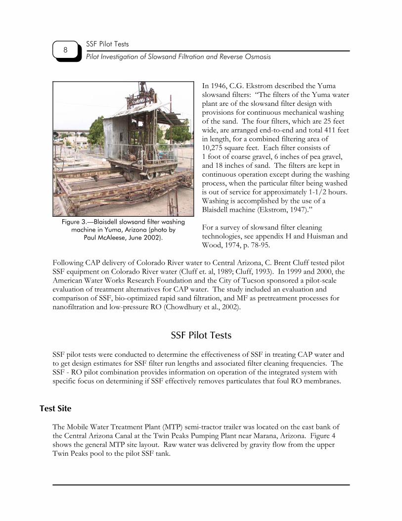
Hiriam W. Blaisdell developed, patented1, and built several slowsand filter washing machines(see figure 3), the first of which was installed in Yuma and operated until 1954 when SSF was replaced with conventional treatment with rapid sand filtration (Doyle & Associates and CarolloEngineering, ca. 1995).

In 1908, William F. Fuller described use of the Blaisdell machine (see figure 3) and slowsandfilter operation at Yuma:

Such a machine has already been in operation at Yuma, Arizona. For 4 or more years, ona slowsand filter, clarifying Colorado River water, having an average turbidity of over2,000 at a rate of 3,000,000 gallons per acre per day, through sand having an effective sizeof 0.13 millimeter, without the use of any coagulants, at a very small maintenance costand with satisfactory results (Fuller, 1908).

8SSF Pilot Tests

Pilot Investigation of Slowsand Filtration and Reverse Osmosis

Figure 3.—Blaisdell slowsand filter washingmachine in Yuma, Arizona (photo by

Paul McAleese, June 2002).

In 1946, C.G. Ekstrom described the Yumaslowsand filters: “The filters of the Yuma waterplant are of the slowsand filter design withprovisions for continuous mechanical washingof the sand. The four filters, which are 25 feetwide, are arranged end-to-end and total 411 feetin length, for a combined filtering area of10,275 square feet. Each filter consists of1 foot of coarse gravel, 6 inches of pea gravel,and 18 inches of sand. The filters are kept incontinuous operation except during the washingprocess, when the particular filter being washedis out of service for approximately 1-1/2 hours. Washing is accomplished by the use of aBlaisdell machine (Ekstrom, 1947).”

For a survey of slowsand filter cleaningtechnologies, see appendix H and Huisman andWood, 1974, p. 78-95.

Following CAP delivery of Colorado River water to Central Arizona, C. Brent Cluff tested pilotSSF equipment on Colorado River water (Cluff et. al, 1989; Cluff, 1993). In 1999 and 2000, theAmerican Water Works Research Foundation and the City of Tucson sponsored a pilot-scaleevaluation of treatment alternatives for CAP water. The study included an evaluation andcomparison of SSF, bio-optimized rapid sand filtration, and MF as pretreatment processes fornanofiltration and low-pressure RO (Chowdhury et al., 2002).

SSF Pilot Tests

SSF pilot tests were conducted to determine the effectiveness of SSF in treating CAP water andto get design estimates for SSF filter run lengths and associated filter cleaning frequencies. TheSSF - RO pilot combination provides information on operation of the integrated system withspecific focus on determining if SSF effectively removes particulates that foul RO membranes.

Test Site

The Mobile Water Treatment Plant (MTP) semi-tractor trailer was located on the east bank ofthe Central Arizona Canal at the Twin Peaks Pumping Plant near Marana, Arizona. Figure 4shows the general MTP site layout. Raw water was delivered by gravity flow from the upperTwin Peaks pool to the pilot SSF tank.

9SSF Pilot Tests


Figu

re 4

.—SA

RWM

S Pi

lot P

lant

, pr

oces

s an

d in

stru

men

tatio

n dr

awin

g (M

obile

Wat

er T

reat

men

t Pla

nt).

10SSF Pilot Tests


Pilot Equipment

The pilot SSF consists of a 16-foot-diameter by 10-foot-high galvanized tank (previously used inthe study by Chowdhury et al., 2002). The SSF tank was placed on a 4-foot high soil pad toelevate the discharge and provide sufficient head for gravity flow to downstream equipment(refer to figure 4). The tank contains perforated polyvinyl chloride (PVC) collection piping at thebottom of 1.5 feet of three (1-inch, 3/4-inch, and 3/8-inch) gravel layers, 3.0 feet of 0.3-milli-meter sand, 4.5 feet of water being filtered, and 1.0 foot of freeboard (see table 2, figures 5(a)and 5(b), and appendix A for a detailed description of the slowsand filter assembly). A geotexfabric layer was installed as a precaution to prevent sand from penetrating into the gravel.

Table 2.—Slowsand filter design1 and pilot operating conditions

Design criteria Full-scale designAugust 7, 2001 -January 2, 2002

January 2, 2002 -March 18, 2002

Period of operation 24 hours/day 24 hours/day 24 hours/day

Product flow 40.14 MGD 22 gal/min(31,680 gal/day)

16 gal/min(23,040 gal/day)

Filtration rate 0.112 gal/min/ft2

0.274 m/h7.0 MGD/acre

0.110 gal/min/ft2

0.269 m/hr6.9 MGD/acre

0.080 gal/min/ft2 0.196 m/hr5.0 MGD/acre

Total filter area 330,450 ft2 or7.6 acres

200 ft2 (16-foot diameter)

200 ft2 (16-foot diameter)

Number of filters 1 with 4 cells at13.38 MGD each

One One

Initial height of filter sand bed 3.0 ft 3.0 ft 3.0 ft

Minimum height of filter sandbed

1.5 ft 1.5 ft 1.5 ft

Sand effective size, d10 0.27 to 0.33 mm 0.27 to 0.31 mm 0.27 to 0.31 mm

Sand uniformity coefficient2,d60/d10

Less than 2.5 1.5 1.5

Height of underdrains, includinggravel layers

1.5 ft 1.5 ft (0.5 ft of 1-in,0.5 ft of 3/4-in, and0.5 ft of 3/8-in gravel)

1.5 ft (0.5 ft of 1-in,0.5 ft of 3/4-in, and0.5 ft of 3/8-in gravel)

Height of supernatant water 5 ft 4.5 ft 4.5 ft

Free board 2 ft 1.0 ft 1.0 ft

Total filter basin depth 11.5 ft 10 ft 10 ft

1 Reclamation, 2000, table E-2, p. E-7. 2 The ratio of the sieve size through which 60 percent of the sand will pass to the size through which 10 percent will pass.

11SSF Pilot Tests


Figure 5(a).—Inflow piping of slowsand tank. The tank is 10 feet tall andhas a diameter of 16 feet.

12SSF Pilot Tests


Figure 5(b).—Outflow piping of slowsand tank.

13SSF Pilot Tests


Figure 6.—SSF outlet flow control structure.

The SSF pilot was operated with “outlet control.” The tank water level was held constant atmaximum height with an inlet float valve. The water height above the initial sand level wasmonitored with a sight tube manometer and is shown as the “SSF inlet level” in appendix B,figure B-8. With an outlet valve, the filter flow was controlled, generally to either 22 or16 gal/min. A second sight tube on the filter outlet (upstream of the control valve) served as amanometer to measure the outlet pressure. This pressure is shown as the “SSF exit level” inappendix B, figure B-8. The difference in water heights of the two manometers is the filterpressure drop and is shown as “SSF dP” in appendix B, figure B-7.

Figure 6 is a photo of the SSF outlet flow control structure. The total flow of 16 or 22 gal/minof SSF-filtered water enters from the 2-inch hose in the center of the photo between thetwo pallets. The total flow ismeasured by the first rotameterflowmeter. The flow then splits,with flow to the right controlled at6 gal/min by a ball valve at thebase of the second rotameter. The rotameters have opaque greensleeves to minimize the growth ofalgae in the clear tubes. To the leftof the 6-gal/min rotameterflowmeter is the sample tap(location SSF-Out) for waterquality analyses of the SSFeffluent. The 6-gal/min flowfrom the rotameter outlet flowsinto the chemical mixing tank andbecomes the “RO feed.”

SSF production in excess of that needed for RO operation flows to the left of the tee. Thisexcess flow (10 or 16 gal/min of filtered water) was returned by natural drainage to the CAPCanal. As the SSF outlet head decreased during a filter run, the gate valve located to the left ofthe tee was gradually opened to maintain SSF flow at 16 or 22 gal/min.

Test Period

The SSF pilot equipment operated 5,000 hours, from August 2001 through March 2002. TheSSF began operation August 7, 2001. After four filter runs for SSF “conditioning,” ROequipment was loaded with membranes, and RO operations began on October 11, 2001.Both SSF and RO equipment operated until March 19, 2002. The SSF equipment operatedcontinuously with planned outages of approximately 8 hours every 3 or 4 weeks at the end of a

14SSF Pilot Tests


filter run when the SSF surface was scraped. The RO equipment was offline during SSFcleanings, during a few short power outages in December 2001, and during two RO cleaningsin January and February 2002.

Water Supply

The water supply to the SSF came from the Central Arizona Project Canal, Twin PeaksPumping Plant discharge pool, gravity siphoned back to the inlet of the SSF tank. CAP wateris dominated by water from the Colorado River, which is pumped from Lake Havasu to Phoenixand then to Tucson.

During the pilot study, the SSF inlet water temperature range was 9 to 24 degrees Celsius (°C)(48 to 75 degrees Fahrenheit) (see appendix B, figure B-4). The TDS of the canal is expected tobe about 700 mg/L (SARWMS, August 2000, table III-7, p. III-10). During the pilot study, theaverage TDS was 670 mg/L (see appendix B, figure B-5). The TOC levels, expected to be about3.5 mg/L (Reclamation, 2000, table III-7, p. III-10) during the pilot study, measured from 2 to7 mg/L, with an average of 3.3 mg/L (see appendix B, figure B-11).

In November 2001, the canal was taken out of service for 3 weeks of maintenance. The pilotequipment was not without water, however, as the upper pool was filled before the shutdown. The quality changed (as indicated by color changing from blue toward green and increased odor)as the canal operations contributed to stagnant water. On December 12, 2001, the turbidityincreased markedly when Twin Peak pumps began to deliver fine black mud in suspension to theupper pool and to the SSF. Because of the proximity of the SSF supply intake, the dischargefrom the Twin Peaks Pumping Plant probably caused localized mixing and increased turbiditylevels (nevertheless, SSF outlet turbidity rarely changed, remaining near 0.2 NTU throughoutthe study). The SSF inlet turbidity levels during the pilot study are shown in appendix B,figure B-9.

Operating Conditions

The pilot SSF was operated at two filtration rates. From August 7, 2001, to August 2002, the200-ft2 pilot SSF operated at 22 gal/min, corresponding to the “high-level” filtration rate of0.110 gal/min/ft2 (0.27 m/h, 6.9 MGD/acre). From January 2, 2002, to March 18, 2002, thepilot SSF operated at 16 gal/min at the mid-level filtration rate of 0.080 gal/min/ft2 (0.20 m/h,5.0 MGD/acre). Table 2 describes the pilot SSF construction and operating conditions and howthese compare with the proposed full-scale design (SARWMS, 2000).

15SSF Pilot Tests


Filtration Rates

During the conditioning phase (August 6, 2001 through September 11, 2001), the filter wasoperated with manual controls by adjusting inlet and outlet valves to achieve constant waterlevel and to maintain 22 gal/min (0.11 gal/min/ft2 through the 200-ft2 filter). For moreconsistent level control, a simple inlet float was installed that maintained the inlet level at55 inches above the initial sand level. On September 11, the outlet rate was set at 22 gal/min,and it was checked frequently. Few (approximately weekly) adjustments to the outlet controlvalve were made during the first 2 weeks of the filter run.

On January 3, 2002, the rate was adjusted to the mid-level filtration rate of 16 gal/min(0.080 gal/min/ft2) to determine if the filtration rate significantly affected the filter run periodand water production.

The SSF pilot was not operated at a planned optional low-level filtration rate of 10 gal/min(0.050 gal/min/ft2, 0.122 m/h, 3.1 MGD/acre) because filtrate quality and filter run lengthswere found acceptable at the mid-level and high-level filtration rates.

Filter Cleaning

The progress of a filter run was tracked by monitoring the filter pressure drop. The filterpressure drop in inches of water head is calculated as the inlet water level (55 inches abovesand as controlled by a float valve) minus the outlet sight tube manometer level.

The SSF component that primarily contributed to the filter pressure drop was the growth andeventual plugging of the schmutzdecke. After each filter scraping removal of the schmutzdecke,the filter pressure drop returned to 5 to 7 inches of water (see appendix B, figure B-8).

When the outlet sight tube manometer level, which was 48 to 51 inches above the sand at thestart of a filter run, approached the level of the sand surface, the SSF was drained to a water level5 to 20 inches below the sand surface. The supernatant water drained via a drain port to a levelof 2 inches above the sand. Draining the last 2 inches through the bed required several (4 ormore) hours. Sometimes areas of water remained perched on top of the schmutzdecke althoughthe sand bed below had drained.

Filter restoration was done by manually scraping the top 3/8 to 1 inch of the filter surface with ahand shovel. The required scraping depth was made obvious by the color contrast of the greenish-black schmutzdecke layer versus the white sand beneath.

Scraping was performed by entering the tank via ladders and shoveling the schmutzdecke intobuckets. Typically, it required 15 buckets and 1 hour of scraping to complete the job. A few

16SSF Results


variations in the scraping methods were tested. Generally, the schmutzdecke was raked intowindrows and then picked up with a shovel. On other occasions, it was shoveled directly intothe buckets. In both cases, the scraped surface was leveled with a shovel and left scored with arake. Raking tended to leave remnants of the schmutzdecke. Shoveling removed more of theschmutzdecke material, but possibly removed excess sand. No effect of the above scrapingvariations was observed on the time required for filter-to-drain following each scraping, waterquality, or filter run length. Except at the end of run 7, permeability upon return to service wasrestored to that the original levels (see the “Filter Run Lengths” section below), indicating thatthe performance was restored to “new” and was independent of method of scraping or rate offiltration. Appendix H describes several mechanized techniques used to clean slowsand filters.

SSF Results

Filter Run Lengths

Filter run lengths and filter run water productions for filter runs 4 - 10 are shown in appendix B,figures B-1 and B-2. Runs prior to run 7 were terminated before the complete head of water wasutilized (see appendix B, figure B-8) to avoid filter cleaning on weekends and holidays.

Table 3 documents the SSF filter run periods, filter run water production, and filterpermeabilities for runs 7 through 10, when the SSF pilot filter was operated to utilize thecomplete head of water. For comparison with values reported for other plants, the SSFparameters are listed in two systems of units.

At the high filtration rate of 0.11 gal/min/ft2 (0.27 m/h, 6.9 MGD/acre), the average filter runperiod for filter runs 7 and 8 was 22 days. At the mid-level filtration rate of 0.08 gal/min/ft2

(0.20 m/h, 5.0 MGD/acre), the average filter run period for filter runs 9 and 10 was 30 days.

Letterman (Logsdon, 1991, p. 151) reports that filter run periods are site specific and have arange of 1 week to 1 year, with an average of about 1.5 months. The August 2000 SARWMSreport (Reclamation, 2000; table E-3 on p. E-10) anticipated a filter run period of 2 months andsix filter cleanings per year at a filtration rate of 0.112 gal/min/ft2 (0.28 m/hr, 7.0 MGD/ acre).At the high filtration rate, the filter run period of 22 days observed in runs 7 and 8 is half the1.5-month average reported by Letterman and one-third the 2-month period anticipated in theAugust 2000 SARWMS report. The costs associated with the shorter filter run periods and morefrequent cleanings are discussed in the “Design and Cost Revisions” section.

Although the run period was shorter with the high-level filtration rate compared to the mid-levelfiltration rate, filter run water production was the same or higher. At the high-level filtration

17SSF Results


Table 3.—SSF filter run periods, filter run water production, and filter permeabilities with 200-ft2 filter

High filtration rate Mid-level filtration rate

Filter run number 7 87and 8average 9 10

9 and 10average

Operating dates Nov. 20, 2001-Dec. 14, 2001

Dec. 14, 2001-Jan. 3, 2002

— Jan. 3, 2002-Feb. 4, 2002

Feb. 4, 2002-March 5, 2002

—

Filtration rate

gal/min 22 22 22 16 16 16

gal/min/ft2 0.110 0.110 0.110 0.080 0.080 0.080

m/h 0.27 0.27 0.27 0.20 0.20 0.20

MGD/acre 6.9 6.9 6.9 5.0 5.0 5.0

Filter run period, days 24 21 22.5 32 29 30.5

Initial filter dP

in H2O 6.5 9 — 5 4 —

m H2O 0.16 0.23 — 0.13 0.10 —

Final filter dP

in H2O 45.5 45 45.2 55.5 54.5 55

m H2O 1.15 1.14 1.15 1.41 1.38 1.40

Water production

gallons 750,600 624,200 687,400 690.900 648,200 669,600

million gallons/acre 164 136 150 151 141 146

m = m3/m2 153.1 127.3 140.2 140.9 132.2 136.6

ft = ft3/ft2 502.3 417.6 460.0 462.3 433.7 448.0

Initial permeability

gal/min/ft2/ inch H2O 0.020 0.012 — 0.020 0.020 —

h-1 1.6 1.2 — 1.5 1.9 —

Final permeability

gal/min/ft2/ inch H2O 0.0024 0.0024 — 0.0015 0.0016 —

h-1 0.23 0.24 0.14 0.14

18SSF Results


rate, the average filter run water production was 140 meters versus 137 meters at the mid-levelfiltration rate (in addition, the 140-meter production occurred with 10 inches less final head (dP)of water across the filter). Both values are at the lower end of the filter run production range of112 to 650 meters reported by Letterman (Logsdon, 1991, p. 151).

Filter Permeability

After each cleaning, the filter permeability was consistently restored to 0.016 to 0.018 gal/min/ft2 per inch of water head (see appendix B, figure B-7). The exception was the December 14,2001, cleaning after filter run 7, indicating incomplete cleaning. Subsequent cleanings after filterruns 8, 9, and 10, however, restored the initial filter permeability to its previous initial levels.

At the high filtration rate of 0.11 gal/min/ft2 (0.27 m/h, 6.9 MGD/acre), the initial SSF pressuredrop at the start of each filter run measured 6 to 7 inches of water (the exception was the startfilter run 8, when on December 15, the pressure drop measured 10 inches of water). At the mid-level filtration rate of 0.08 gal/min/ft2 (0.20 m/h, 5.0 MGD/acre), the initial SSF pressure dropmeasured 4 to 5 inches of water. With a maximum of 4 feet of water above the filter, thesepressure drops for the SSF without schmutzdecke represent 8 to 15 percent of available head.

SSF Filtrate Quality

Twenty six sets of water samples of the SSF inlet and SSF outlet were collected for water qualityanalyses by off-site laboratories (see appendix C, tables C-2 to C-27).

To evaluate the particulate-removal effectiveness of SSF, daily measurements of turbidity and siltdensity index (SDI) were recorded. In addition, the rate of fouling of a downstream pilot ROunit was observed over a 6-month period.

The SSF treatment process does not remove inorganic solutes and TDS. For documentation ofwater compositions, appendix C (tables C-2 to C-7) lists the inorganic water compositions in theSSF feed and product water measured during the study. Levels of TDS, hardness, and pH arediscussed below.

Because of potential oxygen depletion problems at low SSF filtration rates, dissolved oxygenconcentrations were measured daily.

To evaluate the physical disinfection afforded by SSF, heterotrophic plate counts were measuredweekly.

19SSF Results


To evaluate the TOC removal and disinfection byproduct levels that are produced in the SSFproduct, weekly TOC, monthly Trihalomethane Formation Potential (THMFP), and onesimulated distribution system Disinfection Byproduct (SDSDBP) chemical analyses wereconducted.

Turbidity

Turbidity, based on light-scattering, was measured daily with a Hach Turbidimeter 2100Pcalibrated between 20 NTU {clear} and 800 NTU {translucent}. For SSF outlet water, theinstument operated near its generally considered detection limit of 0.1 NTU. Measurementerrors included use of a scratched sample cell before October 30, 2001, fingerprints on thesample cell, a cold sample (relative to the air temperature), causing condensation on the vial, andthe refractive index silicon oil film on the cell being too thick or too thin. These measurementerrors may have contributed to more of the data scatter than any real change in SSF productwater quality.

Appendix B, figure B-9 shows the turbidity levels observed during the study. SSF inlet valuesranged from 0.3 to 24 NTU. The maximum values of 12 and 24 NTU measured at the end ofthe test are higher than the maximum value of 10.2 NTU from 4 years of monthly turbidityreadings of CAP water near the Twin Peaks site.

At Brady (42 miles upstream) and San Xavier (21 miles downstream), from 1998 - 2001, theaverage monthly turbidity was 1.7 NTU and the maximum was 10.2 NTU (Central ArizonaWater Conservation District, 1999-2002). Because these levels are generally less than the10-NTU maximum turbidity level recommended for SSF (AWWA, 1991), CAP water appearsto meet the recommended turbidity criterion for treatment with SSF.

SSF outlet turbidity levels were consistently below 1.0 NTU. Values above 1.0 NTU weremeasured on eight days: five days in October, two days in December, and one day in January (ascratchy sample cell sometimes used before October 30, 2001, is the likely cause of the four highOctober readings). For the period of October 1, 2001, through March 19, 2002, 170 dailyturbidity measurements were recorded (of which seven were greater than or equal to 1 NTU,and 162, or 95.2 percent of the daily measurements, were less than 1.0 NTU). Omitting Octoberdata due to probable measurement errors for the period of November 1, 2001, throughMarch 19, 2002, of 140 measurements, three greater than 1 NTU, and 137, or 97.9 percent, wereless than 1 NTU. Therefore, during this study, SSF treatment of CAP water met the SWTR forturbidity requiring less than 1 NTU for 95 percent of daily samples in a month.

20SSF Results


Silt Density Index

The Silt Density Index (SDI) measurement provides data on concentration and characteristics ofparticulate materials in water. The measurement involves passing water maintained at a constantpressure of 30 pounds per square inch (psi) through a membrane filter with 0.45-micrometer(�m) pore size. As the measurement proceeds, the progressive blockage of the filter pores byparticulates causes the filtration flow rate to decrease. The relative flow decrease yields a percentplugging factor value after a given test duration. SDI is obtained by dividing plugging factor bythe filtration duration. A duration of 15 minutes is standard. If the 15-minute SDI value isgreater than 5, then shorter times of 5 and 10 minutes are used. In this study, SDI values wererecorded with a Chemtec Filter Plugging Analyzer model FPA-3300.

Compared with turbidity, SDI measures lower concentrations of particulates and is generallyused only on filtered water. Therefore, during this study, no SDI measurements of SSFfeedwater were conducted.

Appendix B, figure B-14 shows the SDI values for SSF filtrate and RO feed, where the RO feedlocation is downstream of chemical additions (for a description of chemicals additions, see the“Chemical Feed Systems and Operating Conditions” section) and a 5-�m cartridge filter(Osmonics II GX-05-20). In appendix B, figure B-14 is a horizontal line at SDI of 5. To avoidfouling RO membranes with a coating of particulates, a 15-minute SDI of 5 is the maximumvalue recommended for RO feedwater.

The SDI values were highest immediately after cleaning the SSF filter, sometimes being near 5.0. These anticipated high values generally required a filter-to-drain period of 2 hours (two sandpore volumes) before returning the SSF to RO service. In later cycles, for convenience instarting up the RO equipment during the day, the filter-to-drain period lasted overnight. Duringindividual filter runs, the SDI values improved toward approximately 2.5 at the end of a filterrun. On December 9, 2001, a second SDI unit began measuring SSF outlet upstream ofchemical addition.

Table 4 lists summary statistics for the SDI measurements. Because all statistics presentedassume no dependence between daily samples, and because some dependence is expected, theresults may indicate tighter 95-percent intervals and higher significance than warranted.

For 96 SDI measurements of SSF outlet water from December 8, 2001, through March 19, 2002,the average is 3.59. For 162 SDI measurements of RO feed water from October 9, 2001,through March 19, 2002, the average is 3.90. The average SDI of 3.6 of SSF outlet water iswithin acceptable limits for RO operation.

The chemical additions caused an increase in SDI levels (no biases appeared to be introducedby the different instruments and two sample lines when checked by switching flows to the

21SSF Results


Table 4.—SDI

SSF outletRO feed

(SSF outlet + chemicals)

Dates December 8, 2001 - March 19, 2002 October 5, 2001 - March 19, 2002

Number of measurements 96 162

Mean 3.59 3.90

Standard deviation 1.60 1.06

Standard deviation of the mean 0.126 0.84

95 percent upper bound 3.84 4.06

95 percent lower bound 3.33 3.73

instruments and also by operating with both flows to the same instrument). For 15-minute SDIlevels of 5 and less, the average SDI increase, the SSF outlet, and RO feed for 96 measurementswas 0.45 and was significantly different from zero at the 95-percent confidence level (table 5).

Table 5.—Comparison of 15-minute SDI measurements of less than 5 at two locations

SSF outlet

RO feed(SSF outlet +chemicals)

Difference fromchemical addition

Dates October 5, 2001 -March 19, 2002

October 5, 2001 -March 19, 2002

October 5, 2001 -March 19, 2002

Number of measurements 96 96 96

Mean 3.29 3.74 0.45

Standard deviation 0.84 0.67 0.78

Standard deviation of the mean 0.086 0.068 0.080

95 percent upper bound 3.46 3.88 0.61

95 percent lower bound 3.12 3.60 0.29

RO Fouling Rate

Operation of the pilot RO unit provided information on the effectiveness of SSF in removingparticulates that foul RO membranes. The most sensitive measure of RO fouling is the RO water transport coefficient, “A.” “A” is the proportionality coefficient between the membranewater flux and the driving pressures (hydrostatic and osmotic; see appendix D).

22SSF Results


Because “A” varies with temperature (at approximately 3 percent per °C), “A” is reported at areference temperature of 25 oC using the following temperature correction equation (Beardsley,2001):

tcorr = exp (-3020 x (1 / 298.15) - (1 / (273.15 + T)) (1)

where T is the temperature in °C.

Temperature compensation is critical to evaluating the change in “A” because during the first3 months of RO operation, the temperature decreased 11.3 °C, from 22.4 °C on October 18,2001, to 11.1 °C on January 21, 2002 (see appendix B, figure B-4). Even in the absence offouling, by equation 1, the temperature decrease alone would cause the nontemperature-compensated “A” values to decrease by 33 percent.

Appendix B, figure B-33 shows the “A” values during pilot tests. Table 6 summarizes the valuesof “A” for the RO pilot unit on October 18, 2001 (1 week after startup), before cleaning onJanuary 21, 2002, and at the end of the test on March 19, 2001. During the first 3 months, theaverage of the “A” values for the pilot unit decreased 17 percent, or 8 percent per 1,000 hours ofoperation.

Table 6.—RO water transport coefficient “A” and change in “A” during the pilot test

RO vessel

1 2 3a 3b3

(avg.) Average

Description Date

Operatinghours

(approx.) Parameter Stage 1 Stage 2 Unit

1 week after RO startup 10/18/01 168 A, 10-12 m/s/Pa 23.3 23.4 23.6 22.1 22.8 23.2

Before first cleaning 1/21/02 2,328 A, 10-12 m/s/Pa 20.7 19.1 18.5 17.1 17.8 19.2

Change in “A” after3 mos, % / 3 mos

-11.0% -18% -22% -23% -22% -17%

Change in “A” after3 mos, %/1,000 hrs

-5.2% -8.5% -10% -10.5% -10.2% -8%

At end of test 3/19/02 3,684 A, 10-12 m/s/Pa 24.5 21.7 21.7 19.9 20.8 22.3

Change in “A” after5 mos, % / 5 mos

5% -7% -8% -10% -9% -4%

Change in “A” after5 mos, %/1,000 hrs

1.4% -2.1% -2.3% -2.9% -2.6% -1.1%

23SSF Results


Because of the decline in “A” values, on January 21, 2002, and February 7, 2002, the ROequipment was cleaned at pH 12. The cleaning restored the “A” values to approximately theiroriginal values. The RO pilot test ended after 5 months on March 19, 2002 (with a watertemperature of 13.1 °C). During the 5-month test period, the average of the “A” values for thepilot unit decreased 4 percent, corresponding to a decrease of 1.1 percent per 1,000 hours ofoperation. The 4-percent change between the 1-week and 5-month performances is within theexpected accuracy of flow instrumentation and temperature compensation (see equation 1) and isnot considered significantly different from zero.

A second measure of RO fouling is the pressure drop across each RO stage. Because pressuredrop varies with flow rate and inversely with temperature, an element flow coefficient (Ce;analogous to the valve coefficient Cv) was calculated (see appendix B, figure B-37). AfterOctober 19, 2001, (when interstage pressure lines were connected), Ce for stage 1 remainedsteady at 1.5 gal/min/psid0.6 per element, and Ce for the first three elements in stage 2 (vessel 3a)remained at 1.4 gal/min/psid0.6 per element. Ce for the tail three elements of stage 2 (vessel 3b)decreased approximately 20 percent, from 1.5 to 1.2 gal/min/psid0.6 per element, over the5-month period. Thus, based on Ce values, the RO equipment appeared to experience fouling(and/or scaling) in the tail three elements of stage 2.

In summary, although the initial decline of “A” at the rate 8 percent per 1,000 hours indicatesparticulate fouling, the fouling was apparently effectively removed with two simple high-pHcleanings.

Five weeks after cleaning, and 5 months after startup, the average of the “A” values was only4 percent less than observed at 1 week after startup. Because the initial decline in “A” wasremoved by cleaning, and because after 5 months the values of “A” remained at or near their1-week level, the authors conclude that the pilot SSF served as an effective pretreatment ofColorado River water for removing particulates that foul RO membranes.

Total Dissolved Solids

The TDS (estimated daily from conductivity) of the SSF inlet and outlet waters is shown inappendix B, figure B-5. No difference in TDS was observed between the SSF inlet and outlet.From October 19, 2001 (when the conductivity instrument was calibrated) to March 19, 2002,the average TDS was 673 mg/L. TDS values based on monthly laboratory analyses are listed inappendix C, tables C-2 through C-7.

Hardness

Total hardness is the sum of the calcium and magnesium ion concentrations. For hardnessexpressed as mg/L CaCO3, the relationship is:

24SSF Results


Total hardness [mg/L as CaCO3] = 2.5 x Ca2+ [mg/L] + 4.1 x Mg2+ [mg/L]

Total hardness can also be expressed as grains per gallon (gpg), where 17.12 mg/L as CaCO3equals 1 gpg.

Appendix C, tables C-2 through C-7 list monthly values of hardness, calcium, and magnesium. These are summarized in table 7.

Table 7.—SSF hardness

Date Location Ca2+, mg/L Mg2+, mg/LTotal hardness, mg/L

as CaCO3

August 28, 2001 SSF inlet 68 27 280

SSF outlet 69 27 280

September 25, 2001 SSF inlet 74 28 300


October 25, 2001 SSF inlet 66 28 280


November 19, 2001 SSF inlet 66 29 280


December 17, 2001 SSF inlet 55 26 240


January 15, 2002 SSF inlet 65 27 270


The hardness levels of 240 to 300 mg/L as CaCO3 (14 to 17.5 gpg) correspond to a qualitativeclassification of “hard” water where the four classifications of soft, moderately hard, hard, andvery hard, are listed in table 8. No change in hardness levels was observed between SSF inletand outlet.

SSF pH

In CAP water with calcium and bicarbonate solutes, the natural high pH of about 8.5 reducescorrosion in water pipes. For RO treatment with polyamide (PA) membranes, acid is added toRO feedwater to lower the pH to about 7 to prevent calcium carbonate scaling in the tail ROelements. Because of its low TDS, the pH of the RO product is readily increased to about8.3 by adding a small amount of base (e.g., lime).

25SSF Results


Table 8.—Qualitative classification of waters according tolevel of hardness

(adapted from Sawyer, 1994)

Total hardness

Descriptionmg/L asCaCO3

Grains pergallon

Soft < 50 < 3.0

Moderately hard 50 - 150 3.0 - 9.0

Hard 150 - 300 9.0 - 17.5

Very hard > 300 > 17.5

Appendix B, figure B-12 shows the pH levels of the SSF inlet and outlet. Table 9 summarizesthe pH statistics from November 5, 2001, through March 18, 2002.

Table 9.—SSF pH

SSF inlet SSF outlet SSF reduction

Dates November 5, 2001 -March 19, 2002

November 5, 2001 -March 19, 2002

November 5, 2001 -March 19, 2002


Mean 8.45 8.20 0.25





The average SSF inlet pH was 8.45. The average SSF outlet pH was 8.20. The SSF reduced themeasured pH values by an average of 0.25. This reduction is significantly different from zero atthe 95-percent confidence level.

Similar pH reductions of 0.13 and 0.18 were observed during 1987 pilot SSF tests inNew Hampshire. Collins suggested the respiratory production of carbon dioxide or organicacid intermediates from NOM in the water as a possible cause for the pH reduction (Collinsand Graham, 1994).

The pH reduction could also be caused by the deposition of calcium carbonate solids in the filterbed. This possibility can be explored in future tests with pre- and post-test sand analyses.

26SSF Results


Dissolved Oxygen

Dissolved oxygen (DO) levels of the SSF inlet and outlet streams were measured daily beginningOctober 1, 2001, with a YSI model Y55012 dissolved oxygen meter to monitor oxygen depletionin the SSF outlet. Depletion of the DO within the SSF may create a variable and unstableoperating environment.

The oxygen content is important; if it falls to zero during filtration, anaerobicdecomposition occurs, with consequent production of hydrogen sulfide, ammonia, andother taste- and odor-producing substances together with dissolved iron andmanganese. . . .Thus, the average oxygen content of the filtered water should not beallowed to fall below 3 mg/L if anaerobic conditions are to be avoided throughout thewhole area of the filter-bed (Huisman and Wood, 1974).

Appendix B, figure B-15 shows the daily measurements of DO in the SSF inlet and outlet.Table 10 summarizes DO statistics.

At the high-level filtration rate from October 1, 2001, to January 2, 2002, DO was measured on85 days. The DO concentration in the SSF inlet averaged 7.78. The DO concentration in theSSF outlet averaged 7.34. The water experienced an average reduction of 0.43 mg/L.

At the mid-level filtration rate from January 3, 2002, to March 19, 2002, the DO concentration inthe SSF inlet averaged 7.78 mg/L. The DO concentration in the SSF outlet averaged 7.34. Thewater experienced an average reduction of 0.78 mg/L. At the 95-percent confidence level, thisis significantly greater than the 0.43 mg/L reduction observed at the high-level filtration rate.

The DO depletions of 0.4 mg/L observed at the high-level filtration rate and 0.8 mg/L at thelow-level filtration rate indicate that DO depletion was minor and presented no problem duringthe pilot study.

Operation with warmer summer water at low filtration rates may result in lower DO concentra-tions in the SSF outlet because the solubility of water is less in warm water, and the longerresidence time permits more time for biological activity to deplete the oxygen. Because the studyoperated at mid- and high-level filtration rates, the SSF did not operate under conditions wheresignificant oxygen depletion is likely to occur.

Heterotrophic Plate Count

Weekly water samples were collected for heterotrophic plate count (HPC) analysis of the SSFinlet, SSF outlet, RO feed, RO product, and RO reject streams. The results are shown inappendix B, figure B-10. The primary drinking water standard for HPC is a MCL of 500 bacteriacolony forming units (cfu) per mL. Out of 26 sample collection times, this MCL was exceeded

27SSF Results


Table 10.—SSF dissolved oxygen(mg/L)


High-level filtration rate (0.11 gal/min/ft2, 0.27 m/h, 6.9 MGD/acre)

DatesOctober 1, 2001 -

2002October 1, 2001 -

2002October 1, 2001 -

2002


Mean 7.78 7.34 0.43



95 percent interval upper 7.98 7.51 0.64

95 percent interval lower 7.57 7.18 0.23

Mid-level filtration rate (0.08 gal/min/ft2, 0.20 m/h, 5.0 MGD/acre)

DatesJanuary 3, 2002 -March 19, 2002

January 3, 2002 -Mach 19, 2002

January 3, 2002 -March 19, 2002


Mean 8.45 7.68 0.78





only once (in September 2001) during the pilot study, and that was in the untreated CAPfeedwater (SSF inlet), not the SSF product. Table 11 summarizes the geometric means and95-percent confidence intervals for the SSF inlet and outlet. A geometric mean and logtransformations of the data were used to help create a normal distribution of the data.

The geometric mean HPC values of the SSF inlet and outlet are 48 cfu/mL and 27 cfu/mL for a44-percent reduction. The 95-percent confidence intervals and the t-value of 2.1 indicate thatthe HPC reduction by the SSF is significantly different from zero at the 95-percent confidencelevel.

28SSF Results


Table 11.—SSF heterotrophic plate counts (cfu/mL)

SSF inlet SSF outlet SSF reductiont-value ofreduction

Is reductiondifferent from

zero at the95-percentconfidence

level?

Dates August 28, 2001-February19, 2002

August 28, 2001-February 19, 2002

August 28, 2001-February 19, 2002


Geometric mean 48 27 21 2.1 Yes

95 percent upper bound 76 44 37

95 percent lower bound 31 17 12

SSF Removal of Total Organic Carbon

Although an on-site TOC instrument (Anatel A-2000) was used initially, its use was abandonedon October 9, 2001. Because replicate analyses from the same sample vials producedincreasingly higher TOC values—increasing from 0.5 parts per million (ppm) to 7.0 ppm.

Differences between SSF inlet and outlet TOC values were dwarfed by this analytical variation. Additionally, the instrument sample lines were constructed of very fine capillary tubes—so smallas to be easily blinded by the algae and canal debris in the inlet water samples. After using theinstrument for over 1 month and obtaining inconsistent values, the instrument was taken offline, and samples were sent to an off-site lab for analysis. The off-site lab seemed to have similartroubles, including intermittent measurements of high TOC values in the RO product, wherevery low TOC levels are expected. In summary, TOC measurements did not achieve theexpected levels of accuracy during the study.

Table 12 summarizes the statistics of the weekly SSF TOC measurements from October 9, 2001,to February 19, 2002. The average SSF inlet TOC concentration was 3.3 mg/L. The averageSSF outlet TOC concentration was 2.9 mg/L. The SSF reduced the measured TOC values by anaverage of 0.4 mg/L, or 12 percent. This reduction is significantly different from zero at the95-percent confidence level.

SSF Disinfection Byproduct Levels

Trihalomethane Formation Potential

The THMFP performed per Standard Methods 5710B measures the trihalomethane (THM)concentrations formed during 7 days in the presence of chlorinated water. In the procedure, the

29SSF Results


Table 12.—SSF TOC


Dates October 9, 2001 -March 19, 2002

October 9, 2001 -March 19, 2002

October 9, 2001 -March 19, 2002

No. of measurements 20 20 20

Mean 3.32 2.91 0.41





free chlorine level at the end of the 7-day period is 3 to 5 mg/L. This study uses the THMFPmeasurement to evaluate SSF and RO removals of DBP (specifically THM) precursors. THMand THMFP measurements were performed monthly.

The THM levels of the SSF inlet and outlet (operated without chlorination) were measured as0.0007 mg/L on August 28, 2001, and less than the detection limit of 0.005 mg/L in the otherfive monthly analyses.

Table 13 summarizes the SSF inlet and outlet THMFP levels and the THMFP reductionafforded by SSF. The average SSF inlet THMFP concentration was 0.133 mg/L. The averageSSF outlet THMFP concentration was 0.121 mg/L. The SSF reduced the measured THMFPvalues by an average of 0.013 mg/L, or 10 percent. This reduction is not significantly differentfrom zero at the 95-percent confidence level.

SSF Simulated Distribution System Disinfection Byproducts

Expected in a water treatment plant is post-SSF chlorination for the contact disinfection neededto meet the SWTR for giardia and virus removal and chloramination disinfection for the waterdistribution system. The SWTR requires a combination of filtration and chemical disinfection toprovide 3-log (99.9 percent) reduction of Giardia and 4-log (99.99 percent) reduction of viruses. One way to meet these criteria is SSF and disinfection of the SSF product for 35 minutes with afree chlorine residual of 1.0 mg/L before adding ammonia to form chloramines. The expectedinactivation of Giardia and viruses is shown in table 14.

To estimate the concentrations of DBPs that would be delivered to the consumer with thistreatment, a SDSDBP analysis (Standard Methods 5710C and D) was conducted. For the

30SSF Results


Table 13.—SSF THMFP levels and removals(mg/L)

Date SSF inlet SSF outlet SSF reduction

August 28, 2001 0.236 0.159 0.077

September 25, 2001 0.120 0.114 0.006

October 25, 2001 0.110 0.144 -0.034 (increase)

November 19, 2001 0.133 0.125 0.008

December 17, 2001 0.115 0.103 0.012

January 15, 2002 0.090 0.081 0.009


Mean 0.133 0.121 0.013


Standard deviation of themean

0.021 0.011 0.015


95 percent lower bound 0.079 0.091 -0.025 (increase)

Table 14.—Expected log-removals of Giardia and viruses(AWWA, 1991)

Organism

Treatment Giardia Viruses

SSF 2.0 2.0

Free chlorine (35 minutes at 1.0 mg/L) 1.0 > 4.0

Total 3.0 > 6.0

SWTR requirement 3.0 4.0

Compliance expected Yes Yes

31SSF Results


SDSDBP analysis, water samples were collected February 25, 2002, and delivered to theanalytical laboratory (ATEL, Melmore OH, lab. no. MEL02-02127). The laboratory added1.0 mg/L of free chlorine, added 0.2 mg/L ammonia after 35 minutes to form chloraminedisinfection, and then incubated the sample for 7 days. At the end of the 7-day period, theresidual total chlorine was 0.43 mg/L.

Tables 15 and 16 list the SDSDBP results. At the end of the 7-day period, the TTHM concen-tration (per Environmental Protection Agency [EPA] 524.2) was 0.0147 mg/L (14.7 microgramsper liter [�g/L]), and the total HAA concentration (per EPA 552.2) was 0.0074 mg/L (7.4 �g/L).

Table 15.—SDSTHM(µg/L)

Parameter Concentration Typical

report limit

Chloroform 3.2 0.5

Bromoform 1.7 0.5

Bromodichlromethane 4.4 0.5

Dibromochloromethane 5.4 0.5

Total THM 14.7 2

Table 16.—SDSHAA(µg/L)

ParameterResult(µg/L )

Typical reportlimit

Bromochloroacetic acid 3.1 1

Dibromoacetic acid 2.6 1

Dichloroacetic acid 1.7 1

Monobromoacetic acid <1.0 1

Monochloroacetic acid <1.0 1

Trichloroacetic acid <1.0 1

Total HAA 7.4 6

32SSF Results


These concentrations are less than the MCLs listed by the SDWA Stage 1 D/DBPR. Themeasured SDSTHM of 0.0147 mg/L is 18 percent of the 0.080 mg/L MCL for TTHM. Themeasured SDSHAA of 0.0074 mg/L is 12 percent of the 0.060 mg/L MCL for HAA5.

Because the SDSDBP procedure had less than the intended 1.0-mg/L free chlorineconcentration at the end of the initial 35 minutes, the measured SDSDBP concentrationsreported above underestimate the DBP levels associated with the intended disinfection. Withhigher chlorine dosages of 2.0 to 2.5 mg/L (instead of 1.0 mg/L) and contact times longer than35 minutes, the SDSDBP concentrations are expected to be higher but probably still less thanthe DBP MCLs. To confirm or correct the SDSDBP concentrations, SDSDBP analyses shouldbe repeated in future tests.

SSF Post-Test Sand Inspection

Upon completion of the pilot test, the sand was inspected. Several core samples were obtainednear the center of the tank. Test pits were dug at the center and near the outside circumference. The test pits and core samples were visually examined, and gradations were run on several of thesamples. See appendix A for pictures taken during the examination.

The visual analysis of both core samples and test pits indicated that the sand cross-section belowthe schmutzdecke appeared unaltered. The schmutzdecke layer, about one-half inch thick, wasclearly visible due to the slightly darkened appearance. No signs of piping or channeling wereseen in any of the test pits.

Gradations were performed at the near-surface (schmutzdecke layer), at a depth of 2 feet, and ata depth of 3 feet. The surface layer gradation contained a slightly higher fines content of1.3 percent compared to a pretest gradation reading of 0.5 percent fines. The 2- and 3-footdepth gradations indicated a fines content of 0.3 percent, compared with a pretest averagereading of 0.5 percent.

In summary, there appeared to be essentially no change in the fines content of the sand based onpre- and post-pilot gradation analyses. The fines content in the top schmutzdecke layerincreased slightly as would be expected. The gradations at depth indicated fewer fines than atpretest, possibly due to flushing action during the test. No piping or channeling of the flowthrough the filter cross-section was observed. The flow through the filter matrix was evidentlyvery uniform.

The sand used in the pilot test provided a very effective filter. Very little (if any) migration orpenetration of fines was observed.

33Reverse Osmosis Description


Reverse Osmosis Description

RO pilot equipment was operated to evaluate the effectiveness of SSF for removing particulatesthat foul RO membranes. The RO pilot equipment was also operated to demonstrate operationof the complete SSF - RO process, document RO solute removals and product water composi-tions, and determine if disinfection of the RO product can use free chlorine without ammoniaand still meet the SDWA Stage 1 D/DBPR of 0.080 mg/L TTHM and 0.060 mg/L of HAA5.

RO is a barrier process that uses hydraulic pressure to overcome the osmotic pressure of the feedflow. Osmosis is a natural process whereby water is transported through a semipermeablemembrane from a solution of low concentration to one of high concentration. For example, iffresh water and salty water are separated by a semipermeable membrane, the fresh water willtend to move through the semipermeable membrane in an attempt to equalize the saltconcentrations of the waters on both sides of the membrane. This tendency produces a drivingforce that operates in a manner similar to pressure. The term “osmotic pressure” is used todescribe it.

RO operates by applying sufficient pressure on the feedwater (salty) side of the membrane toforce water through the membrane to the fresh water side, thus reversing the osmotic process. The pressure required depends on several factors, including the TDS salinity of the feedwater, temperature of the feedwater, the membrane water transport coefficient, the design membraneflux (gallons of permeate per square foot of membrane per day [gfd]), and the water recovery. Recovery is the percentage of feedwater recovered as RO product. RO membranes permit verylittle passage of dissolved salts so that the RO product TDS is much lower than the feedwaterTDS.

Another aspect of RO as a barrier process is it rejects other contaminants in the feedwater inaddition to dissolved salts. RO rejects not only Giardia and Cryptosporidium, but also viruses,dissolved salts, and many organic solutes (often measured as TOC). Because many organicsolutes form DBPs when free chlorine is used for disinfection, RO removal of these DBPprecursors greatly reduces the levels of DBPs in the finished water. Present and proposedregulations for THM, HAA, and DBPs are readily met with RO treatment. Because of the verylow DBP levels, use of free chlorine (instead of chloramine) becomes an option for disinfectionof the finished water.

There are several types of RO membranes that can be used. The selection of the appropriatemembrane for a particular case depends on the TDS level of the feedwater and the permeatequality goals. “Nanofiltration” is a form of RO that is useful in softening hard water. Nano-filtration membranes are most effective in rejecting divalent ions (ions with a positive or negativecharge of two) such as calcium, magnesium, and sulfate. Typically, rejection rates for divalentions are in excess of 95 percent, whereas the rejection rates for monovalent ions (ions with a

34Reverse Osmosis Description


single charge) are much lower (approximately 50 to 70 percent). Nanofiltration typically operatesat feedwater pressures of about 80 to 100 psi. Depending on the feedwater quality, permeaterecoveries of 80 percent or more are common.

For treatment of Colorado River water with a TDS of about 700 mg/L, low-pressure ROmembranes appear to have the appropriate combination of low to moderate operating pressuresand moderate salt rejection. Applicable commercial RO membranes include DOW FilmTecmodel NF90 (where NF indicates nanofiltration RO), Fluid Systems model TFC ULP (whereULP indicates ultra-low pressure RO), and Hydranautics model ESPA 3 (a.k.a. ESNA). Therecommended RO design in the SARWMS report was based on the FilmTec NF90 membraneprojections with fouling allowances estimated from pilot tests conducted by Reclamation withthe City of Tucson (Reclamation, 2002).

Particulates in feedwater, as well as microbiological growth in the RO equipment, can coat or“foul” RO membranes. Fouling causes loss of flux and/or an increase in operating pressure. Fouling can sometimes be removed by cleaning, but at additional costs. If the fouling coatingseverely restricts the passage of water and cannot be removed, the resulting low-water fluxand/or high operating pressures require premature replacement of the RO membranes.

The RO membrane chemistry type selected in the August 2000 SARWMS design and operatedin the pilot test is PA. PA membranes operate at lower pressures and have correspondinglylower energy costs than cellulose acetate (CA) membranes.

PA membranes are much more sensitive than CA membranes to fouling by particulates in thefeedwater. Because membrane fouling results in higher operating pressures, it can partially offsetsome of the energy savings associated with PA membranes and may require frequent cleaning.

For pilot tests evaluating the effectiveness of SSF in removing particulates that foul ROmembranes, the fouling sensitivity of PA membranes provides a stricter standard than would CAmembranes. If PA membranes can operate with low fouling with SSF pretreatment, then one would expect that CA would operate with much lower fouling. Membrane manufacturerscontinue to develop improved PA membranes with increased resistance to chlorine degradationand fouling.

For treating Colorado River water, less acid is need with PA membranes than with CAmembranes, which require water acidification to about pH 5.5. PA membranes, however,degrade in the presence of free chlorine.

A critical design parameter for inland desalting plants is water recovery, the percentage ofproduct water that is recovered from the feedwater. Achieving the highest water recoverypossible without precipitation (scaling) of sparingly soluble solutes in the concentrate is generallythe goal for inland sites and for brackish (waters with TDS of 3,000 to 10,000 mg/L) and lower

35SSF - RO Pilot Process Description


salinity waters. Water recovery is a critical design parameter because high recovery correspondsto high utilization of the feedwater supply and to low volumes of waste concentrate to bedischarged.

The design water recovery is 85 percent. Recovery appears to be limited by barium sulfatesolubility (barium and sulfate concentrations in the design CAP Canal water are 10 times bariumsulfate solubility). A conservative estimate of maximum barium sulfate concentration in thereject stream is 60 times solubility. When a mix of Colorado River water and Aqua Fria Riverwater (from Lake Pleasant) is delivered with a TDS of 700 mg/L, 60 times solubility corresponds to a water recovery of 72 to 79 percent. At the design 85 percent recovery andfeed pH adjusted to 7.2 with sulfuric acid, the barium sulfate concentration is about 120 timessolubility.

The CAP Canal operation includes periods when 100 percent of Colorado River water isdelivered (Central Arizona Water Conservation District, 1997, 1998). With the Colorado Riverwater composition, barium sulfate remains the principal scaling compound of concern. At85-percent recovery and feed pH of 7.2, the barium sulfate concentration is about 130 timessolubility.

Based on pilot test results at the Hayden-Udall Water Treatment Facility and the Water QualityImprovement Center, operation at 85-percent water recovery (at 120 to 130 times the solubilityof barium sulfate) appears feasible with the use of antiscalants. Higher water recoveries may beachievable but require confirmation with additional high-recovery pilot tests on Colorado Riverwater.

The design water flux is 12 gfd, and the intent was to operate the pilot RO equipment at 12 gfdbased on FilmTec Product Information listing a membrane area of 23 square feet for 2.5-inch-diameter by 40-inch-long RO elements. The membrane area, however, has apparently beenincreased because the DOW FilmTec website (http://www.dow.com/liquidseps/pc/nfe.htm) asof June 6, 2002, lists an active element area of 28 square feet for NF90-2540 elements. Post-testdissections of two NF90-2540 test elements measured an active membrane area of 25.4 squarefeet. With 25.4 square feet of membrane area per element, the RO equipment operated at10.9 gfd.

SSF - RO Pilot Process Description

A flow schematic of the pilot SSF - RO process is shown in figure 4. The pilot SSF is containedin a 16-foot-diameter tank and has an area of 200 square feet. SSF feedwater was drawn fromthe CAP Canal at the discharge of the Twin Peaks pumping station in Marana, Arizona. Nochemical treatments (e.g., disinfection or coagulation) were used on the SSF feed.



Between the SSF outlet and feed to the RO processes, four chemicals were added. Antiscalant(Ecolab Flocon 100) was added to prevent scaling by barium sulfate. Sulfuric acid (J.T.BakerCMOS 9684-05; 95 - 97 percent H2SO4) was used to adjust the RO feed pH from about 8.3 to 7.0 to avoid scaling by calcium carbonate. Bleach (Clorox, 6 percent) was used for chlorinationdisinfection. Ammonium sulfate (Fisher A702-10 technical grade) was added to combine withthe free chlorine to produce chloramine disinfection.

The August 2000 SARWMS report (Reclamation, 2000) describes a 24-MGD (27,000 acre-feetper year) RO design with a water recovery of 85 percent. Because three-stage RO equipment isrecommended for achieving greater than 80-percent recovery, and because the MTP pilot systemhas only two stages, a water recovery of 80 percent was used during the pilot tests.

The pilot test was not designed to address biological fouling of commercial PA membranesoperated with no disinfectant in the RO feedwater. Because commercial PA membranes areconsidered susceptible to damage and loss of salt-rejection with chlorinated water, they are notpresently recommended for operation on chlorinated or chloraminated water. For this short-term study, however, to obtain an accurate picture of particulate fouling in the absence ofbiological fouling, chloramine disinfection was used in the RO feedwater.

Chemical Feed Systems and Operating Conditions

The chemical feed systems consist of four ProMinent diaphragm metering pumps (ProMinentGala and g/4b), two static mixers (Chemineer Kenics HEV-6) in a 30-gal/min mixing loop (referto figure 4). On the suction side of the RO feed pump, four chemicals are added in a specificorder: antiscalant, acid, bleach, ammonia (see figures 7 - 10). These were added in a rapidlyflowing mixing loop. The order of addition was considered important. Because adding sulfuricacid adds sulfates, which could begin forming barium sulfate scale, the antiscalant was addedupstream of the acid injection point. This mixture was then passed through a static mixer. Sulfuric acid was added to lower the pH from 8.3 to 7.0 to prevent calcium carbonate scaling. Next, Clorox brand bleach was injected. For operation with polyamide membranes, ammoniumsulfate is added to convert free chlorine to chloramine disinfection. The pumped mixing loopwas used to provide adequate flow through the static mixers and served to externally mix the150-gallon RO feed tank (table 17).

The process flow is 6.0 gal/min. Dilution water is RO product with less than 25-mg/L TDS andwith chloramine residual.

Post-test review of the doses listed in table 17 revealed that 1/10th the intended dose was usedfor the antiscalant because of a dilution error. The dilution error resulted in an antiscalant doseof 0.4 mg/L instead of the intended 3.6 mg/L and may have contributed to scaling indicatedby the analyses of solids scraped from the tail element (see the “Scaling” section below).



Table 17.—Chemical feed operating criteria and doses

Concentration(percent)

Criteria and dose of100 percent chemical

Chemical Source Neat Diluted Criteria

Dose

mL/min mg/L

Antiscalant Ecolab Flocon100

100 0.5 3.6 mg/L 1.8 0.4

Sulfuric acid J.T.Baker CMOS9684-05

95 - 97 5.2 pH = 7.0 5.0 15

Sodium hypochlorite Clorox 6 1.0 1.0 to1.5 mg/Lresidualchlorine

3.15 1.4

Ammonia(ammonium sulfate)

Fisher A702-10technical grade

26 as NH3 1.2 Excess NH3 4.0 2.2

RO Pilot Plant Operation

Reverse Osmosis Equipment and Operating Conditions

The MTP RO equipment consists of a series of six 2.5-inch, 3-element pressure vessels thatcontain a total of 18 membrane elements in a 12:6 element (and 2:1 6-element vessel) array (referto figure 4). A VFD pump boosts the feed pressure to about 90 psi, where the feedwater splitsto feed vessel 1a & 1b (V1) and vessel 2a and 2b (V2). The pressurized concentrate from V1and V2 feeds V3. V1 and V2 each contain six 2.5-inch-diameter by 40-inch-long “2540" spiral-wound NF90 elements by Dow FilmTec. Water which passes through the RO membranetravels through a spiral path and collects into a center product water tube. The feedwater whichdoes not permeate through the first element leaves the annular space of the first element andenters the annular passages of the second element. This inter-element water is at slightly lowerpressure than seen by the first element and slightly more concentrated—being deprived of the



Figure 8.—Acid feed system (sulfuric acid), with spill pallet,17-gallon supply tank, calibration cylinder, and back pressure valve.

Figure 7.—Antiscalant feed system (Flocon 100) with spill pallet,5-gallon supply tank, calibration cylinder, and back pressure valve.



Figure 9.—Chlorine feed system (bleach), with spill pallet,17-gallon supply tank, calibration cylinder, bypass relief line,

pulsation dampener, and back pressure valve.

Figure 10.—Ammonia feed system (ammonia sulfate), withspill pallet, 17-gallon supply tank, calibration cylinder, bypass

relief line, pulsation dampener, and back pressure valve.



permeate water produced by the first element. At slightly lower hydrostatic pressure, ca. 11 per-cent higher osmotic pressure, and ca. 11-percent higher feed salinity, each succeeding identicalelement produces slightly less permeate water and with higher salinity than the permeate water ofthe preceding element.

As RO product water is produced from the six elements of V1, it is collected into a commonproduct tube and directed to a sample sink. Just prior to entering the sink, it encounters a needlevalve which controls the RO product back pressure and hence the volume of RO product. Thedischarge from the needle valve is measured by a rotameter flowmeter.

The rotameter calibration was checked by graduated cylinder, stopwatch, and mass scale. Fromthis mass measurement, a rotameter float set point was determined, and frequent RO productflow rate checks could be made quickly and accurately. In the pilot RO unit, the product valveswere used to approximately equalize element product flows for both stages. In a full-scale ROplant, interstage booster pumps may be used to increase pressures by about 30 psid per stage tocompensate for the hydrostatic pressure drop across each stage and for the higher osmoticpressure of the feedwater in each succeeding stage.

The flow through V2 also encountered six elements and produced P2 RO product. Theinterstage concentrate from V1 and V2 enters V3a, which has three elements and produces ROproduct as P3a. The second stage concentrate from V3a enters V3b and produces P3b ROproduct and the final rejected concentrate as R.

The RO reject and four product flows were controlled by manually adjusting the reject valve (aflow control valve on V3b discharge), the four RO product valves, and the VFD speed. When the system production was affected by water temperature, fouling, or cleaning, flow rates weremaintained approximately constant by daily adjustments to the RO reject and four RO productvalves and infrequent (three times during the 5-month test) adjustments to the RO feed pumpVFD.

A portion of the RO product was diverted and collected in a RO product tank. During normaloperations, RO product was measured and then discharged back to the CAP Canal.

RO Startup, Cleaning, and Shutdown Procedures

When starting the RO equipment after installing new elements, or restarting after being down formore than 4 hours, the process started at low pressure and flow to purge the RO equipment ofair bubbles. Initially, the feed-forward pump operated at about 30 psi with the reject valve fullyopen and the RO product valves closed. After about 5 minutes, the reject and RO productvalves were brought to about 80 percent of their normal operating positions. After recheckingthe chemical metering systems, the VFD pump was ramped up (taking about 5 minutes to reach



full speed). Flow control valves and pump speed were adjusted in rapid rotation to achieve thespecified product and reject flows (table 18). As flows and pressures increased, the sound ofremaining air in the equipment was noticeable. After this 15-minute startup sequence, thesystem would be nearly stable. Minor changes continued to occur during the next 4 hours.After this startup, the system usually remained stable for weeks before the next adjustment wasrequired.

Table 18.—Reverse osmosis pilot equipment flow ratesetpoints for 80-percent water recovery

Stream locationFlow rate setpoint

(L/min)

Feed 16.32

Reject 3.26

Total product 13.06

Product, stage 1

Vessel 1 (six elements) 4.35

Vessel 2 (six elements) 4.35

Product, stage 2

Vessel 3a (three elements) 2.39

Vessel 3b (three elements) 1.96

Because of the observed decline in water transport coefficient “A” during the first 3 months ofthe test, the RO equipment was cleaned in January and February. With SSF pretreatment andthe absence of iron or aluminum coagulants, high-pH cleaning solutions were used to addressfouling by organic matter.

On January 21, 2002, an 18-gallon batch of chlorine-free RO product was heated to 20 °C andadjusted to pH 12 with sodium hydroxide (Red Devil lye). This solution was circulated throughthe RO system at low pressure and high velocity.

Because the target water temperature of 30 °C (see appendix E) was not achieved, on February 7,2002, a second cleaning was conducted with RO product at pH 12 and 30 °C.

42Reverse Osmosis Results


Prior to both cleaning events, the RO equipment operated without chloramine disinfection toproduce RO product water free of chloramines. The cleaning solutions were circulated forseveral hours, while maintaining the original temperature with stainless steel immersion heaters(Cole Parmer U-03046-50). During the January 21 cleaning, foaming and minor amounts ofparticulates (pepper flake in appearance) appeared in the return line (these particulates couldhave come from the action of the cleaner on dirty rubber circulation hoses). During theFebruary 7 cleaning, the water was slightly foamy but remained clear with a slight tea color.

When the RO equipment was shut down for SSF cleaning, it was flushed with collected ROproduct until the reject concentration was essentially equal to inventoried RO productconcentration. This flush took approximately 15 minutes and three system volumes at5 gal/min. (one system volume is approximately 15 gallons). The RO equipment operated atlower pressure after each RO flush, as described in the “Reverse Osmosis Results” section.

The RO reject (concentrate) water was discharged into an evaporation bed. Figure 4 shows theSARWMS pilot plant process and instrumentation drawing for the MTP.

Reverse Osmosis Results

Operating conditions and performance are shown in figures in appendix B. Water compositions,mass balance checks, and solute removals are listed in tables in appendix C.

Membrane Equations

To monitor and evaluate RO equipment performances under varying feedwater and operatingconditions, mathematical descriptions of the RO process can be used to try to eliminateoperational variations to get a clearer description of the performance of the RO equipment atconstant operating conditions. Sometimes called “normalization” equations, the equations usedin this report, as well as a symbol list and sample calculations, are described in appendix DWQIC Reverse Osmosis Equations.

Appendix D also describes mass balance equations used to check RO flows and watercomposition listed in appendix C.

Water Flows, Compositions, and Operating Pressures

To maintain RO product membrane fluxes of 10.9 gfd and 80-percent water recovery, the ROfeed and RO product pressures were adjusted. The RO feed flow was maintained at 16.3 L/min



(4.31 gal/min). The total RO product was maintained at 13.06 L/min (3.45 gal/min). The ROreject (concentrate) flow was maintained at 3.26 L/min (0.86 gal/min), which is slightly less thanthe minimum 3.8 L/min (1.0 gal/min) recommended by the manufacturer.

The RO pilot equipment operated with a maximum hydrostatic pressure difference of 644 kilo-pascals (90 psid) across the RO membranes (see appendix B, figure B-31). This maximumpressure occurred December 14, 2001, the coldest day of the test, with a feedwater temperatureof 8.9 oC.

Tables 21, 22, and 23 summarize the RO performance at the start of the test, after 3 months,and at the end of the test. For comparison, the tables also show the DOW FilmTec Reverse Osmosis System Analysis (ROSA) version 5.0 prediction for the RO pilot unit. Although theROSA program lists an active membrane area of 28 square feet per element, post-test dissectionof two test elements measured an active membrane area of 25.4 square feet per element.

The RO product TDS estimated from conductivity on the three dates ranged from 15 to23 mg/L, approximately 30 percent of the 55- to 79-mg/L levels predicted by ROSA. Theindividual solute concentrations in the RO product were frequently less than the laboratorydetection limit, and none exceeded the ROSA predictions.

RO pilot equipment pressure measurements were used to estimate the ROSA fouling factorwhere a fouling factor of 1.0 corresponds to “new” membrane elements and a positive value lessthan 1.0 corresponds to fouled elements. At 2 weeks after startup, the estimated fouling factor is0.81 (see table 19). After 3 months and observed fouling, the estimated fouling factor is0.70 (see table 20). At the end of the test after 5 months of operation and 5 weeks after a pairof cleanings, the estimated fouling factor is 0.86 (see table 21). The final fouling factor of0.86 indicates that the high-pH cleanings conducted in the 4th month (January and February)were effective in removing deposited foulants and restoring RO operation to “near new”performance.

Fouling – RO Fouling Rate

The ROSA fouling factors estimated above (see tables 21, 22, and 23) of 0.87 at 2 weeks afterstart and 0.75 at 3 months after start indicate that the RO equipment required higher operating pressures due to fouling over the first 3 months. The estimated fouling factor of0.93 at 5 months after start (and 5 weeks after cleaning) indicates that the RO performance wasrestored to better than at 2 weeks after start.

As described above under the SSF “RO Fouling Rate,” section, the most sensitive measure ofRO fouling is the RO water transport coefficient “A” at a reference temperature of 25 °C. “A”is the proportionality coefficient between the membrane water flux and the driving pressures,


Pilot Investigation of Slowsand Filtration and Reverse Osmosis TreatmentTa

ble

19.—

Com

paris

on o

f obs

erve

d an

d pr

ojec

ted

RO p

erfo

rman

ce a

t beg

inni

ng o

f tes

t

Dat

eTe

st p

erio

dC

onfig

urat

ion

Feed

tem

pera

ture

, °C

Prod

uct f

low

, gal

/min

Feed

flow

, gal

/min

Wat

er r

ecov

ery

Oct

ober

25,

200

12

wee

ks a

fter

star

tEi

ghte

en N

F90-

2540

ele

men

ts in

a 2

:1 a

rray

of 6

-ele

men

t ves

sels

20.9

3.46

4.31

80.4

%

Mea

sure

dRO

SA p

redi

ctio

n

Wat

er c

ompo

sitio

nRO

feed

RO p

rodu

ctRO

rej

ect

RO fe

edRO

pro

duct

RO r

ejec

t

Bica

rbon

ate

- H

CO

3 (m

g/L)

Cal

cium

- C

a (m

g/L)

Chl

orid

e -

Cl

(mg/

L)M

agne

sium

- M

g (m

g/L)

Pota

ssiu

m -

K (m

g/L)

Silic

a -

SiO

2 (m

g/L)

Sodi

um -

Na

(mg/

L)St

ront

ium

- S

r (m

g/L)

Sulfa

te -

SO

4 (m

g/L)

Tota

l dis

solv

ed s

olid

s -

TDS

(mg/

L)TD

S (re

sidu

e at

180

°C

) (m

g/L)

TDS

estim

ated

from

con

duct

ivity

(mg/

L)La

b pH

(S.U

.)

61 65 65 28 6 8 88 2 260

581

690

694

6.8

8.54 <4

7.8

<3

<5

0.4

7.3

<0.

2<

5<

41.9

130

22.8

5.2

281

290

310

130

30 39 390 9

1,20

02,

666

3,00

02,

943

7.3

61 65 147

28 6 8 88 2 260

685

685

685

6.8

16.8

1.1

26.1

0.3

1.5

1.2

22.0

0.02 3.0

72.0

72.0

72.0

4.6

240

324

457

140

26 35 356 8

1,30

22,

891

2,89

12,

891

7.5

Mea

sure

dA

djus

ted

to m

atch

mea

sure

d pr

essu

res

Pres

sure

s, p

sig

8232

.5(s

tg. 1

)21

.5(s

tg. 2

)69

8532

.5(s

tg. 1

)21

.5(s

tg. 2

)61

ROSA

foul

ing

fact

or e

stim

ated

from

m

easu

red

pres

sure

s0.81

N

ote:

To

achi

eve

ion

bala

nce

in th

e RO

feed

wat

er, t

he R

OSA

pro

gram

add

ed 4

6 m

g/L

of c

hlor

ide.


Pilot Investigation of Slowsand and Reverse Osmosis TreatmentTa

ble

20.—

Com

paris

on o

f obs

erve

d an

d pr

ojec

ted

RO p

erfo

rman

ce m

idw

ay th

roug

h te

st

Dat

eTe

st p

erio

dC

onfig

urat

ion

Feed

tem

pera

ture

, °C

Prod

uct f

low

, gal

/min

Feed

flow

, gal

/min

Wat

er r

ecov

ery

Janu

ary

15, 2

002

3 m

onth

s af

ter

star

tEi

ghte

en N

F90-

2540

ele

men

ts in

a 2

:1 a

rray

of 6

-ele

men

t ves

sels

13.3

3.45

4.35

79.5

%

Mea

sure

dRO

SA p

redi

ctio

n

Wat

er c

ompo

sitio

nRO

feed

RO p

rodu

ctRO

rej

ect

RO fe

edRO

pro

duct

RO r

ejec

t

Bica

rbon

ate

- H

CO

3 (m

g/L)

Cal

cium

- C

a (m

g/L)

Chl

orid

e -

Cl

(mg/

L)M

agne

sium

- M

g (m

g/L)

Pota

ssiu

m -

K (m

g/L)

Silic

a -

SiO

2 (m

g/L)

Sodi

um -

Na

(mg/

L)St

ront

ium

- S

r (m

g/L)

Sulfa

te -

SO

4 (m

g/L)

Tota

l dis

solv

ed s

olid

s -

TDS

(mg/

L)TD

S (re

sidu

e at

180

°C

) (m

g/L)

TDS

estim

ated

from

con

duct

ivity

(mg/

L)La

b pH

(S.U

.)

61 64 59 27 6.1

6.9

86 1.7

250

560

520

685

6.8

1.22 4 3.8 3 5 0.6 5 0.2 5

28.6

20 14.8

4.8

262

300

270

120

27 30 380 9

1,10

02,

486

2,60

02,

905

7.3

61 6411

0.8

27 6.1

6.9

86 1.7

250

614

614

614

6.8

13.1

0.9

19.7

0.2

1.1

0.8

16.6

0.01 2.1

55.0

55.0

55.0

6.2

247

309

464

131

25 31 355 8

1,21

12,

784

2,78

42,

784

7.5

Mea

sure

dA

djus

ted

to m

atch

mea

sure

d pr

essu

res

Pres

sure

s, p

sig

9426

(stg

1)

6(s

tg. 2

)78

9826

(stg

. 1)

6(s

tg. 2

)70

ROSA

foul

ing

fact

or e

stim

ated

from

m

easu

red

pres

sure

s0.70

N

ote:

To

achi

eve

ion

bala

nce

in th

e RO

feed

wat

er, t

he R

OSA

pro

gram

add

ed 5

2 m

g/L

of c

hlor

ide.



Tabl

e 21

.—C

ompa

rison

of o

bser

ved

and

proj

ecte

d RO

per

form

ance

at e

nd o

f tes

t

Dat

eTe

st p

erio

dC

onfig

urat

ion

Feed

tem

pera

ture

, °C

Prod

uct f

low

, gal

/min

Feed

flow

, gal

/min

Wat

er r

ecov

ery

Mar

ch 1

9, 2

002

5 m

onth

s af

ter

star

tEi

ghte

en N

F90-

2540

ele

men

ts in

a 2

:1 a

rray

of 6

-ele

men

t ves

sels

13.1

3.44

4.34

79.3

%

Mea

sure

dRO

SA p

redi

ctio

n

Wat

er c

ompo

sitio

nRO

feed

RO p

rodu

ctRO

rej

ect

RO fe

edRO

pro

duct

RO r

ejec

t

TDS

est.

from

con

duct

ivity

(mg/

L)69

418

.82,

499

685

60.0

3,05

5

Fiel

d pH

(S.U

.)7.

05.

97.

37.

06.

37.

7

Mea

sure

dA

djus

ted

to m

atch

mea

sure

d pr

essu

res

Pres

sure

s, p

sig

9333

(stg

. 1)

15(s

tg. 2

)76

9733

(stg

. 1)

15(s

tg. 2

)69

ROSA

foul

ing

fact

or e

stim

ated

from

m

easu

red

pres

sure

s0.86

N

ote:

Bec

ause

the

RO fe

ed c

ondu

ctiv

ity v

alue

s w

ere

the

sam

e on

Oct

ober

25,

200

1, a

nd M

arch

19,

200

2, th

e O

ctob

er 2

5, 2

002,

RO

feed

wat

er c

ompo

sitio

n w

as u

sed

in th

e RO

SA p

redi

ctio

n fo

r M

arch

19,

200

2.



both hydrostatic and osmotic, and its calculation is described in appendix D. High values of “A”correspond to high membrane water flux and/or low feed pressure. For the pilot test operatedat constant RO product flow, high values of “A” correspond to low feed pressure. Appendix B,figure B-33 shows the values of “A” during the pilot test.

During the first 3 months (see table 6), the average of the “A” values for the pilot unit decreased17 percent, or 8 percent per 1,000 hours of operation.

Because of the decline in “A” values, on January 21, 2002, and February 7, 2002, the ROequipment was cleaned at pH 12. The cleaning restored the “A” values to approximately theiroriginal values. The RO pilot test ended after 5 months on March 19, 2002. During the5-month test period, the average of the “A” values for the pilot unit decreased 4 percent,corresponding to a decrease of 1.1 percent per 1,000 hours of operation (see table 6). The4-percent decrease in performance between the beginning of the test (1-week after start) and theend of the test 5 months later is within the expected accuracy of flow instrumentation andtemperature compensation (see equation 1) and is not considered significantly different fromzero.

Another measure of RO fouling is the pressure drop across each RO stage. Because pressuredrop varies with flow rate and inversely with temperature, an element flow coefficient (Ce;analogous to the valve coefficient Cv) was calculated (see appendix B, figure B-37). AfterOctober 19, 2001, (when interstage pressure lines were connected), Ce for stage 1 remainedsteady at 1.5 gal/min/psid0.6 per element, and Ce for the first three elements in stage 2 (vessel 3a)remained at 1.4 gal/ min/psid0.6 per element. Ce for the tail three elements of stage 2 (vessel 3b)decreased approximately 20 percent, from 1.5 to 1.2 gal/min/psid0.6 per element, over the5-month period. Thus, based on Ce values, fouling was not observed in stage 1 or the leadthree elements of stage 2. Based on a 20-percent decrease in Ce values for vessel 3b, the ROequipment appeared to experience fouling in the tail three elements of stage 2.

In summary, fouling was evident during the first 3 months of operation. The estimated ROSAfouling factor decreased from 0.81 to 0.70, for a relative decrease of 14 percent. This decrease isconsistent with the change in calculated “A” values, which decreased by 17 percent.

Although the initial declines of fouling factor and “A” at the rate of 7 percent and 8 percent per1,000 hours indicates particulate fouling, the fouling was apparently effectively removed with twosimple high-pH cleanings. Five weeks after cleaning and 5 months after startup, the estimatedfouling factor was 0.93 (higher than the 0.87 value at 2 weeks after start), and the average of the“A” values was only 4 percent less than observed at 1 week after start. Because the initial declinein fouling factor and “A” was removed by cleaning, and because after 5 months the values offouling factor and “A” remained at or near their initial 1- and 2-week levels, we conclude that thepilot SSF served as an effective pretreatment of Colorado River water for removing particulatesthat foul RO membranes.



Scaling

In the RO process, the feedwater becomes more concentrated between the lead and tailmembrane elements. The high concentrations in the tail elements may cause precipitation outof solution of sparingly soluble solutes. This precipitation is called “scaling.” Whereas foulingcoats the membrane with particulates already in the feedwater, scaling coats the membrane withparticulates formed within the RO equipment. Scaling and fouling have similar operationaleffects, but initially, scaling generally occurs only in the tail elements. For CAP water, scale-forming compounds of concern are barium sulfate, calcium sulfate, strontium sulfate, andcalcium carbonate. Organic solutes from dissolved natural organic matter and organicantiscalant may also possibly precipitate out of solution and coat the RO membrane.

The values of “A” declined during the first 3 months, and the rate of decline was somewhathigher in stage 2 than in stage 1 (see table 6 and appendix B, figure B-33). The stage 2 decreasein “A” could be from either fouling or scaling.

The value of Ce for stage 2 decreased 20 percent during the test while the value of Ce for stage 1did not decrease (see appendix B, figure B-37). The stage 2 decrease in Ce could be from eitherfouling or scaling.

Mass balance deviations (MBDs) with high positive values may indicate deposition of soluteswithin the RO equipment and are another indication of scaling. The MBDs for mineral andorganic solutes in four monthly chemical analyses are listed in appendix C, tables C-4, C-5, C-6,and C-7.

Barium levels are generally below detection in the RO feed, so the MBD for barium cannot becalculated.

The highest MBD for calcium was calculated for October 25, 2001, to be between 7.5 and12.4 percent. This is within the accuracy of the chemical analysis and the flow measurementsand is not considered significant.

All MBDs for sulfate are less than 10 percent.

None of the MBDs for strontium are positive.

Organic solutes from dissolved natural organic matter and organic antiscalant may possiblyprecipitate out of solution and coat the RO membrane. The MBDs for TOC are listed inappendix C, figures C-2 through C-25 and C-27. On six dates (October 25, 2001; November 19,2001; December 4, 2001; December 17, 2001; January 15, 2002; and February 19, 2002), theMBDs for TOC are positive (with an average bracket of 13 to 29 percent). On the other dates,



the TOC is zero (within the accuracy of the measurements) or negative. With both positive andnegative MBDs for TOC, the MBD does not indicate a deposition of TOC in the ROequipment.

Appendix F describes post-test dissections of one lead element (from vessel 1) and one tailelement (from vessel 3b). The tail element operated at approximately 50 percent lower waterflux and processed approximately 50 percent less water during the pilot test. Scrapings of oneleaf (with an area of 12.7 ft2 = 1.18 m2 ) measured 5.6 times the mass of solids on the tail element than on the lead element. After drying at 105 °C, the density of solids calculated was70.1 mg/m2 ( = 82.7 mg/1.18 m2 ) for the lead element and 393 mg/m2 ( = 464 mg/1.18 m2 )for the tail element.

Eleven times the mass of carbon compounds was found on the tail element compared to thelead element. The difference in mass between drying at 105 °C and 600 °C is called “loss onignition (LOI)” and provides an estimate of the carbon compound content of the solids. TheLOI measured 31 percent for the lead element and 62 percent for the tail element (seeappendix F, “Membrane Foulant Analysis”). Assuming that all of the LOI consists of carboncompounds, then the density of carbon compounds scraped from the membranes can becalculated as 22 mg/m2 ( = 0.31 x 70.1 mg/m2 ) for the lead element and 244 mg/m2

( = 0.62 x 393 mg/m2 ) for the tail element.

Possible sources of carbon compounds include NOM in the water and antiscalant. Calciumcarbonate may also be present, but a high concentration of calcium carbonate is consideredunlikely because of the success in cleaning the RO membranes at pH 12.

The inorganic analyses indicate possible scaling with barium sulfate, calcium sulfate, andstrontium sulfate. Appendix F, figures F-1 and F-2 summarize the results of inductively coupledplasma (ICP) analyses of the solids after drying at 600 °C. Scaling of the tail element is indicatedbecause the barium, calcium, and strontium mass concentrations in appendix F, figure F-1 aregreater than ten times higher for the tail element than for the lead element. The sulfurconcentration is four times higher for the tail element than for the lead element.

In summary, ICP analyses of solids scraped from the lead and tail elements indicate possiblescaling of the tail element by barium sulfate, calcium sulfate, and strontium sulfate. This isconsistent with the observations of somewhat higher rates of decline for “A” and Ce in stage 2than in stage 1. In contrast, the MBDs do not indicate scaling.

Because ICP analysis of solids scraped from the tail element indicates that scaling may haveoccurred at a water recovery of 80 percent and because incorrectly low levels of antiscalant wereused, further tests are needed to evaluate RO water recovery levels that are achievable withoutscaling. Monitoring of the performance of the individual tail element in future tests can providemore sensitive and rapid detection of changes in “A” due to scaling.



Salt Passage

Appendix B, figure B-29 shows the RO salt passage calculated from TDS values estimated fromdaily conductivity measurements. Because the RO equipment operated at constant water flow,salt passage varies with water temperature. The salt passage of the FilmTec NF90 elementsmeasured 2.4 to 3.0 percent with a water temperature of 21.8 °C at the start of the test and 1.3 to1.9 percent with a water temperature of 13.1 °C at the end of the 5-month test. With thecoldest water temperature of 8.6 °C on December 14, 2001, the salt passages measured 1.0 to1.5 percent.

Salt passage measures membrane desalting performance, and significant increases in salt passagewould indicate degradation, for example from chloramine disinfection or cleaning. The stabilityof the salt passage values do not indicate degradation.

A similar RO performance parameter that does not vary with temperature is the ratio of the saltand water transport coefficients. The parameter “B/A” (see appendix B, figure B-35) exhibited atemporary increase following cleaning. This increase could indicate membrane degradation. Nevertheless, the final values of B/A approximately equal the initial values and do not indicatedegradation. Further tests with repeated cleanings are recommended to determine if cleaningadversely increases salt passage and B/A.

RO Solute Removal

Appendix C, tables C-4 through C-7 list the concentrations of solutes in the RO feed, product,and reject waters and the calculated RO removals of solutes for four dates: October 25, 2001,November 19, 2001, December 17, 2001, and January 15, 2002. Appendix B, figure B-26 alsoshows TDS levels estimated from daily conductivity measurements. Discussed below are TDS,hardness, TOC, and THMFP. See appendix C, tables C-4 through C-7 for other compositionmeasurements.

Based on measured concentrations listed in appendix C, tables C-4 through C-7 and on expectedRO removal of contaminants not analyzed, RO product concentrations meet all primary andsecondary drinking water standards for inorganic contaminants.

TDS Removal

The RO product TDS measured 31 mg/L at the start of the test, 10 mg/L on December 14,2001, and 19 mg/L at the end of the 5-month test (see appendix B, figure B-26). At constant



production, higher TDS levels of 50 to 60 mg/L would occur in the summer. These TDS levelsreadily meet the secondary drinking water standard of 500 mg/L for TDS and are less than theapproximately 200-mg/L TDS levels in area groundwater.

With a feed TDS of 670 mg/L and a reject TDS of approximately 3,000 mg/L (see appendix B,figure B-27), the RO removal of TDS during the test ranged from 97 to 99 percent (note thatRO removal of TDS equals 100 percent minus salt passage discussed above).

Appendix C, tables C-4 through C-7 list TDS levels measured by evaporation at 180 °C. Becauseof the low TDS levels in the RO product, however, the authors consider TDS estimated fromconductivity to provide more accurate values for the RO product.

Hardness

With 250 to 280 mg/L hardness in the RO feed and 1,200 to 1,400 mg/L hardness in the ROreject, the RO product hardness measured less than the 22-mg/L laboratory detection limit on allfour dates (see appendix C, tables C-4 through C-7). These levels correspond to greater than95.4 to 96.0 percent removal of hardness (based on average feed and reject concentrations). TheRO product hardness level places the RO product in the “soft” water classification (see table 8).

RO Removal of Total Organic Carbon

With 2.8 to 3.9 mg/L TOC in the RO feed and 9.3 to 13 mg/L in the RO reject, the ROproduct TOC measured less than the 0.5-mg/L laboratory detection limit on all four dates (seeappendix C, tables C-4 through C-7). These levels correspond to greater than 90.3 to93.2 percent removal of hardness (based on average feed and reject concentrations).

Disinfection Byproduct Measurements

With chloramine disinfection, the TTHM concentrations in the RO feed, RO product, andRO reject measured less than the 1.0-�g/L laboratory detection limit on all four dates (seeappendix C, tables C-4 through C-7).

To obtain estimates of RO removal of THM precursors and to determine if disinfection withfree chlorine alone (without ammonia addition to form chloramines), THM formation potential(THMFP) measurements were conducted. THMFP measures the THM concentrations after7 days of storage with a final free chlorine concentration of 3 to 5 mg/L.

52Design and Cost Revisions


With 85 to 138 �g/L total THMFP in the RO feed and 148 to 208 �g/L in the RO reject, theRO product total THMFP measured 0.9 to 3 �g/L (see appendix C, tables C-4 through C-7). These levels correspond to 98.9 to 99.6 percent removal of hardness (based on average feed andreject concentrations).

The total THMFP levels of 0.9 to 3 �g/L in the RO product are much less than the MCLs listedby the SDWA Stage 1 D/DBPR of 80 �g/L TTHM. In addition, the THMFP 7-day freechlorine levels of 3 to 5 mg/L are much higher than the 0.5 to 1.0 mg/L required fordisinfection of water distribution systems. For these two reasons, with RO product water-freechlorine alone (without ammonia addition to form chloramines) can be used as the disinfectantand meet the SDWA D/DPR MCL for TTHM.

Design and Cost Revisions

Based on these pilot tests, no major changes are recommended to the SSF design described inappendix E of the August 2000 report (Reclamation, 2000).

During pilot tests, the SSF was run to exhaustion and cleaned when the schmutzdecke becameplugged. Draining the bulk of supernatant was accomplished quickly through a drain valve, butthe final dewatering of the top few inches of sand media required several hours. To avoid thisdelay, the supernatant filter drain should be designed to drain all of the supernatant water.

The appraisal-level estimates of O&M labor costs (Reclamation, 2000, tables E-5 and E-6) arebased on using a single operator for a 42-MGD facility. Many activities at a water treatmentfacility, however, require at least two persons for safe and efficient operations. For this reason,and to accommodate the increased SSF cleaning frequency from 6 to 17 times per year (seebelow), the revised estimate includes increased labor costs for a staff of three operators. Thischange increases the labor cost from $41,600 per year to $124,800 per year.

The August 2000 SARWMS report (Reclamation, 2000, table E-3, p. E-10) estimates a sand filtercleaning frequency of six times a year. Based on pilot results with 22-day filter runs (refer toappendix B, figure B-1, runs 7 and 8), the estimated sand filter cleaning frequency has beenincreased to 17 times per year. The higher SSF cleaning frequency is estimated to increase costsof sand replacement by a factor of 17/6 per year.

Appendix G incorporates the increased costs of labor and sand replacement which, in turn,increase the total O&M costs. For SSF treatment without desalting, the estimated total of theO&M costs for administration and chemistry laboratory, SSF, and finished water reservoirincreases from $ 0.24 million per year to $ 0.41 million per year (see table 22 and appendix G,figure G-3). The increased O&M cost changes the estimated unit cost of SSF-treated water from$0.13 per thousand gallons to a revised estimate of $0.15 per thousand gallons.


Pilot Investigation of Slowsand and Reverse Osmosis TreatmentTa

ble

22.—

Trea

tmen

t alte

rnat

ives

sum

mar

y

Varia

ble-

prod

uctio

n pl

ant t

o m

eet p

eak-

day

40.1

4-M

GD

cap

acity

, 26.

76-M

GD

ave

rage

, and

67-

perc

ent p

lant

fact

or (4

5,00

0 AF

Y)

Trea

tmen

tAn

nual

and

uni

t cos

ts

Con

figur

atio

nC

osts

$mill

ion/

year

$/1,

000

gallo

ns

Cap

ital c

osts

($ m

illio

n)O

&M

cos

ts ($

mill

ion/

year

)C

AP-C

T46

.97

1.67

3.93

1.67

0.57

Cap

ital c

osts

($ m

illio

n)O

&M

cos

ts ($

mill

ion/

year

)C

AP-S

SF12

.35

0.41

1.03

0.41

0.15

Cap

ital c

osts

($ m

illio

n)O

&M

cos

ts ($

mill

ion/

year

)C

AP-M

F/U

F59

.80

0.54

5.01

0.54

0.57

Con

stan

t-pro

duct

ion

plan

t with

ASR

for

23.9

5-M

GD

ave

rage

, 26.

76-M

GD

pea

k ca

paci

ty, a

nd 9

5-pe

rcen

t pla

nt fa

ctor

(30,

000

AFY)

Trea

tmen

tC

once

ntra

te d

ispo

sal

Annu

al a

nd u

nit c

osts

Con

figur

atio

nC

osts

Alte

rnat

ive

Cos

tsTo

tal c

osts

$mill

ion/

year

$/1,

000

gal

Cap

ital c

osts

($ m

illio

n)O

&M

cos

ts ($

mill

ion/

year

)a.

Pipe

line

to P

uerto

Pen

asco

(with

no

partn

ers)

75.0

20.

2013

2.35

3.53

10.5

13.

531.

61

Cap

ital c

osts

($ m

illio

n)O

&M

cos

ts ($

mill

ion/

year

)b.

Evap

orat

ion

pond

s62

.96

0.07

120.

293.

409.

593.

401.

49

Cap

ital c

osts

($ m

illio

n)O

&M

cos

ts ($

mill

ion/

year

)C

AP-C

T-RO

57.3

23.

32

c.Pi

pelin

e to

Pue

rto P

enas

cow

ith 1

7.6

MG

D fr

om T

ucso

n15

.50

0.04

72.8

23.

365.

983.

361.

07

Cap

ital c

osts

($ m

illio

n)O

&M

cos

ts ($

mill

ion/

year

)d.

CAS

I pip

elin

e to

Yum

aw

ith 3

7.6

MG

D fr

om T

ucso

n an

d SR

OG

48.6

40.

1310

5.96

3.45

8.50

3.45

1.37

Cap

ital c

osts

($ m

illio

n)O

&M

cos

ts ($

mill

ion/

year

)e.

CAS

I can

al to

Yum

aw

ith 3

7.6

MG

D fr

om T

ucso

n an

d SR

OG

28.4

70.

2385

.79

3.56

6.96

3.56

1.20

Cap

ital c

osts

($ m

illio

n)O

&M

cos

ts ($

mill

ion/

year

)f.

CAS

I can

al to

Yum

aw

ith 2

72-M

GD

tota

l flo

w13

.72

0.01

71.0

43.

335.

843.

331.

05

Cap

ital c

osts

($ m

illio

n)O

&M

cos

ts ($

mill

ion/

year

)a.

Pipe

line

to P

uerto

Pen

asco

(with

no

partn

ers)

75.0

20.

2010

9.95

2.72

8.63

2.72

1.30

Cap

ital c

osts

($ m

illio

n)O

&M

cos

ts ($

mill

ion/

year

)b.

Evap

orat

ion

pond

s62

.96

0.07

97.8

92.

597.

712.

591.

18

Cap

ital c

osts

($ m

illio

n)O

&M

cos

ts ($

mill

ion/

year

)C

AP-S

SF-R

O34

.93

2.51

c.Pi

pelin

e to

Pue

rto P

enas

cow

ith 1

7.6

MG

D fr

om T

ucso

n15

.50

0.04

50.4

22.

554.

102.

550.

76

Cap

ital c

osts

($ m

illio

n)O

&M

cos

ts ($

mill

ion/

year

)d.

CAS

I pip

elin

e to

Yum

aw

ith 3

7.6

MG

D fr

om T

ucso

n an

d SR

OG

48.6

40.

1383

.56

2.64

6.62

2.64

1.06

Cap

ital c

osts

($ m

illio

n)O

&M

cos

ts ($

mill

ion/

year

)e.

CAS

I can

al to

Yum

aw

ith 3

7.6

MG

D fr

om T

ucso

n an

d SR

OG

28.4

70.

2363

.40

2.75

5.09

2.75

0.90

Cap

ital c

osts

($ m

illio

n)O

&M

cos

ts ($

mill

ion/

year

)f.

CAS

I can

al to

Yum

aw

ith 2

72-M

GD

tota

l flo

w13

.72

0.01

48.6

52.

523.

972.

520.

74



Tabl

e 22

.—Tr

eatm

ent a

ltern

ativ

es s

umm

ary

(con

tinue

d)

Con

stan

t-pro

duct

ion

plan

t with

ASR

for

23.9

5 M

GD

ave

rage

, 26.

76 M

GD

pea

k ca

paci

ty, a

nd 9

5-pe

rcen

t pla

nt fa

ctor

(30,

000

AFY

) (co

ntin

ued)

Trea

tmen

tC

once

ntra

te d

ispo

sal

Annu

al a

nd u

nit c

osts

Con

figur

atio

nC

osts

Alte

rnat

ive

Cos

tsTo

tal c

osts

$mill

ion/

year

$/1,

000

gal

Cap

ital c

osts

($ m

illio

n)O

&M

cos

ts ($

mill

ion/

year

)a.

Pipe

line

to P

uerto

Pen

asco

(with

no

partn

ers)

75.0

20.

2013

4.76

2.88

10.7

12.

881.

55

Cap

ital c

osts

($ m

illio

n)O

&M

cos

ts ($

mill

ion/

year

)b.

Evap

orat

ion

pond

s62

.96

0.07

122.

702.

759.

792.

751.

43

Cap

ital c

osts

($ m

illio

n)O

&M

cos

ts ($

mill

ion/

year

)C

AP-

MF/

UF-

RO59

.74

2.68

c.Pi

pelin

e to

Pue

rto P

enas

cow

ith 1

7.6

MG

D fr

om T

ucso

n15

.50

0.04

75.2

42.

726.

182.

721.

02

Cap

ital c

osts

($ m

illio

n)O

&M

cos

ts ($

mill

ion/

year

)d.

CAS

I pip

elin

e to

Yum

aw

ith 3

7.6

MG

D fr

om T

ucso

n an

d SR

OG

48.6

40.

1310

8.38

2.81

8.70

2.81

1.32

Cap

ital c

osts

($ m

illio

n)O

&M

cos

ts ($

mill

ion/

year

)e.

CAS

I can

al to

Yum

aw

ith 3

7.6

MG

D fr

om T

ucso

n an

d SR

OG

28.4

70.

2388

.21

2.91

7.17

2.91

1.15

Cap

ital c

osts

($ m

illio

n)O

&M

cos

ts ($

mill

ion/

year

)f.

CAS

I can

al to

Yum

aw

ith 2

72-M

GD

tota

l flo

w13

.72

0.01

73.4

62.

696.

042.

691.

00

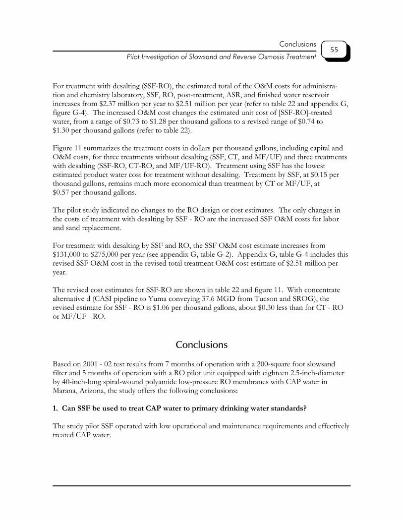
55Conclusions


For treatment with desalting (SSF-RO), the estimated total of the O&M costs for administra-tion and chemistry laboratory, SSF, RO, post-treatment, ASR, and finished water reservoirincreases from $2.37 million per year to $2.51 million per year (refer to table 22 and appendix G,figure G-4). The increased O&M cost changes the estimated unit cost of [SSF-RO]-treatedwater, from a range of $0.73 to $1.28 per thousand gallons to a revised range of $0.74 to$1.30 per thousand gallons (refer to table 22).

Figure 11 summarizes the treatment costs in dollars per thousand gallons, including capital andO&M costs, for three treatments without desalting (SSF, CT, and MF/UF) and three treatmentswith desalting (SSF-RO, CT-RO, and MF/UF-RO). Treatment using SSF has the lowestestimated product water cost for treatment without desalting. Treatment by SSF, at $0.15 perthousand gallons, remains much more economical than treatment by CT or MF/UF, at$0.57 per thousand gallons.

The pilot study indicated no changes to the RO design or cost estimates. The only changes inthe costs of treatment with desalting by SSF - RO are the increased SSF O&M costs for laborand sand replacement.

For treatment with desalting by SSF and RO, the SSF O&M cost estimate increases from$131,000 to $275,000 per year (see appendix G, table G-2). Appendix G, table G-4 includes thisrevised SSF O&M cost in the revised total treatment O&M cost estimate of $2.51 million peryear.

The revised cost estimates for SSF-RO are shown in table 22 and figure 11. With concentratealternative d (CASI pipeline to Yuma conveying 37.6 MGD from Tucson and SROG), therevised estimate for SSF - RO is $1.06 per thousand gallons, about $0.30 less than for CT - ROor MF/UF - RO.

Conclusions

Based on 2001 - 02 test results from 7 months of operation with a 200-square foot slowsandfilter and 5 months of operation with a RO pilot unit equipped with eighteen 2.5-inch-diameterby 40-inch-long spiral-wound polyamide low-pressure RO membranes with CAP water inMarana, Arizona, the study offers the following conclusions:

1. Can SSF be used to treat CAP water to primary drinking water standards?

The study pilot SSF operated with low operational and maintenance requirements and effectivelytreated CAP water.

56Conclusions


1.32

1.06

1.37

0.57

0.15

0.57

0.00

0.20

0.40

0.60

0.80

1.00

1.20

1.40

1.60

CT SSF MF/UF CT-RO SSF-RO MF/UF-RO

$/10

00 g

allo

ns

Figure 11.—Estimated CAP water treatment costs revised to include increased SSF labor and sandreplacement cost estimates. For treatments with desalting, concentrate disposal costs are based on aCentral Arizona Salinity Interceptor (CASI) pipeline to Yuma conveying 37.6 MGD from Tucson and theArizona Municipal Water Users Association Sub-Regional Operating Group (SROG).

57Conclusions


During this study, SSF treatment of CAP water met the SWTR for turbidity requiring lessthan 1 NTU for 95 percent of daily samples in a month.

Expected disinfection in a water treatment plant is post-SSF chlorination disinfection to meetthe SWTR for giardia and virus removal and chloramination disinfection for the waterdistribution system. With lower free chlorine concentration than specified to achieve 4-loggiardia removal, the 7-day SDSDBP levels from one analysis measured 0.015 mg/L forTTHM and 0.007 mg/L for HAA5. These levels are much less than the SDWA Stage 1D/DBPR MCLs of 0.080 mg/L TTHM and 0.060 mg/L HAA5. With higher free chlorineconcentrations, we expect the SDSDBP levels to be higher but still meet the TTHM andHAA5 MCLs.

Based on TOC and THMFP measurements, SSF does not greatly reduce DBP precursorconcentrations. SSF removed 0.4 mg/L, or 12 percent of the TOC. SSF reduction ofTTHMFP was not statistically significant at the 95-percent confidence level.

2. How effective is SSF as a pretreatment to RO?

SSF treatment of CAP water appears adequate for removing particulates that foul reverseosmosis polyamide membranes. SSF should also to provide adequate pretreatment for celluloseacetate membranes, which were not tested but generally foul much less than polyamidemembranes. Although the initial decline of membrane water transport coefficient “A” at therate of 8 percent per 1,000 hours indicates particulate fouling, two simple high-pH cleaningseffectively restored the “A” values. Five weeks after cleaning, and 5 months after startup, theaverage of the “A” values was only 4 percent less than observed at 1 week after startup.

3. What is the salinity and composition of CAP water treated by SSF and RO?

During the pilot test, the RO product TDS measured 10 to 31 mg/L, hardness measured lessthan 22 mg/L, and TOC measured less than 0.5 mg/L. Based on results listed in appendix C,water treated by SSF - RO meets all primary and secondary drinking water standards forinorganic contaminants.

4. For disinfection of RO product, can free chlorine without ammonia be used to meetthe SDWA Stage 1 D/DBPR MCLs of 0.080 mg/L TTHM and 0.060 mg/L of HAA5?

Based on very low measured total THMFP levels of 0.001 to 0.003 mg/L in the RO product,free chlorine without ammonia be used to meet the MCL for TTHM and most probably alsomeet the MCL for HAA5.

58Recommendations


5. What changes to SSF costs estimated in the August 2000 SARWMS are indicated bythe pilot tests?

The estimated cost of SSF treatment is revised to $0.15 per 1,000 gallons, increased from the$0.13 per 1,000 gallons estimated in the August 2000 SARWMS report (Reclamation, 2000). Theincrease is based on cleaning the SSF 17 times per year (every 21 days) as required with the pilotSSF at the high filtration rate of 0.11 gal/min/ft2 (0.27 m/h, 6.9 MGD/acre). The August 2000SARWMS report assumed six cleanings per year.

Recommendations

Because SSF effectively treats CAP water at one-fourth the cost of either CT or MF/UF, subjectto future tests demonstrating successful year-round operation, the authors recommend SSF forCAP water treatment without desalting.

For CAP water treatment with desalting, the authors recommend two alternatives. Onealternative is MF/UF in combination with low-pressure RO. The second alternative,recommended subject to the successful completion of additional pilot tests, is SSF incombination with low-pressure RO.

Because SSF has significantly lower costs than CT, MF treatment, or UF treatment, and becausethe present pilot test has demonstrated the effectiveness of SSF filtration during 7 months ofoperation and SSF has little operational flexibility once constructed, the authors recommendfollowing the advice of Leland and Logsdon to conduct pilot tests for at least 1 year (Logsdon,1991, p. 194). Because SSF cleaning costs represent 60 percent of the estimated O&M costs, theauthors also recommend evaluating SSF cleaning technologies. The recommended pilot testsand evaluation of cleaning technologies should address the following questions:

(1) What are the effects of a range of seasonal (i.e., spring and summer) CAP waterconditions on SSF filtrate quality, filter run lengths, and filter run production volumes?

(2) What are the effects of using locally available sand with a different size and uniformitycoefficient than the sand used in the present pilot study (shipped from California) onSSF filtrate quality, filter run lengths, and filter run production volumes?

(3) What SSF filtration rates provide filter runs lasting at least 1 month over a range of CAPwater conditions, and what are the associated filter run production volumes?

(4) How effective are mechanized SSF cleaning technologies, and which technologies appearmost cost-effective?

59Recommendations


(5) What are the effects of changes in water conditions and SSF loading rates on SSFeffluent DO, HPC, pH, TOC, and SDSDBP levels and on effluent particulate levels asindicated by turbidity, SDI, and fouling rates of RO pilot equipment?

(6) What range of combinations of filtration rates and cleaning frequency appear mostpractical when used with mechanized SSF cleaning technologies?

For RO treatment of CAP water, the authors recommend pilot tests to address the followingquestions:

(7) To ensure that the apparently successful RO cleanings conducted during the pilot testsdo not damage the RO membranes, what are the effects of multiple high-pH, high-temperature RO cleanings on RO salt passage?

(8) Can RO pilot equipment be operated at the plant design recovery of 85 percent withoutscaling? To provide more sensitive and rapid detection of changes in “A” due to scaling,include instrumentation to monitor the performance of the tail RO element.

pilot investigation of slowsand filtration and reverse ... · pilot investigation of slowsand...

Documents