physics - i laboratory manual for engineering undergraduates
TRANSCRIPT

BURSA ULUDAĞ UNIVERSITY FACULTY OF ARTS & SCIENCE - 2019
PHYSICS - I LABORATORY MANUAL FOR ENGINEERING
UNDERGRADUATES

i
Contents 0. ERROR ANALYSIS ........................................................................................................................... 1
0.1. Error ............................................................................................................................................. 1
0.2. Absolute Error .............................................................................................................................. 1
0.3. Relative Error ............................................................................................................................... 2
0.4. Arithmetical Mean ........................................................................................................................ 2
0.5. Standart Error in the Mean Value ................................................................................................. 2
0.6. The Error in a Single Measurement with a Tool .......................................................................... 2
0.7. Error in Composite Quantities ...................................................................................................... 2
0.8. Error Calculation in Fundamental Algebra .................................................................................. 3
0.9. Calculating Error of a Quantity measured over a Graphic ........................................................... 3
1. MOTION IN ONE DIMENSION ....................................................................................................... 5
2. SIMPLE PENDULUM ...................................................................................................................... 10
3. ANALYSIS OF A SPRING .............................................................................................................. 15
4. CONSERVATION OF ENERGY ..................................................................................................... 19
1
0. ERROR ANALYSIS
0.1. Error
All experimentally determined physical quantities contain some degree of error or uncertainty. The error
in a measurement is defined as the difference between the measured value and the real value of a physical
quantity determined in the experiment.
The numerical value of a measured physical quantity cannot be expressed with its real value due to the
experimental errors. The sensitivity and the confidentiality of a measurement are determined with the
level of errors, which occur in experiments. An experimental result does not have any scientific meaning
unless the error level is provided. Thus, the error, which arises in measurements of the experimental
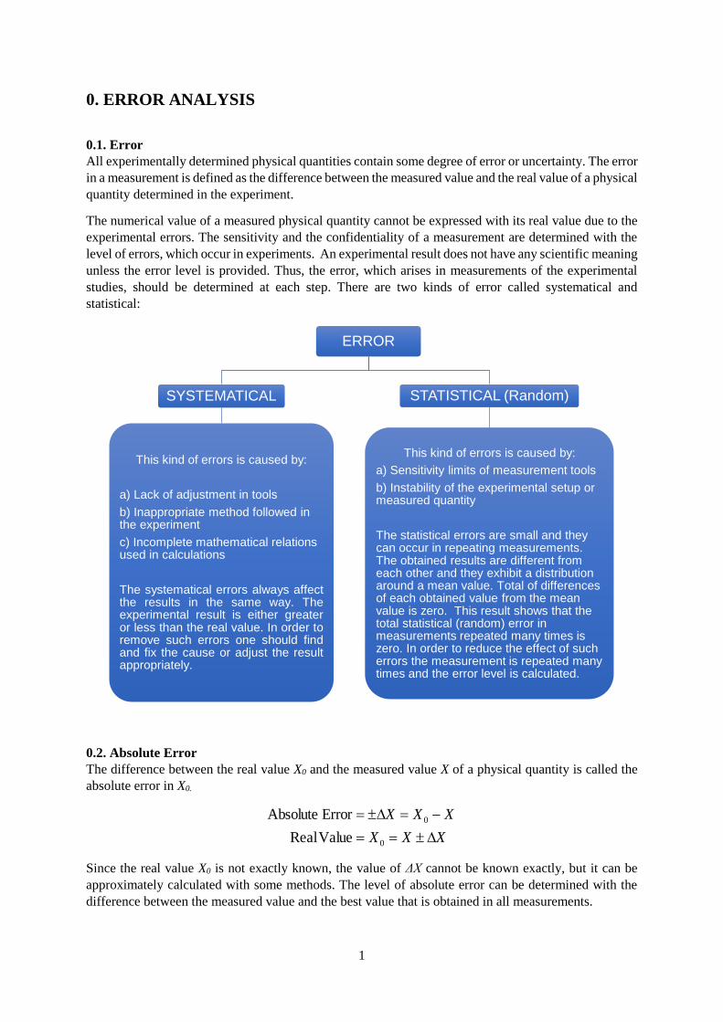
studies, should be determined at each step. There are two kinds of error called systematical and
statistical:
0.2. Absolute Error
The difference between the real value X0 and the measured value X of a physical quantity is called the
absolute error in X0.
XXX
XXX
0
0
ValueReal
ErrorAbsolute
Since the real value X0 is not exactly known, the value of ΔX cannot be known exactly, but it can be
approximately calculated with some methods. The level of absolute error can be determined with the
difference between the measured value and the best value that is obtained in all measurements.
ERROR
SYSTEMATICAL
This kind of errors is caused by:
a) Lack of adjustment in tools
b) Inappropriate method followed in the experiment
c) Incomplete mathematical relations used in calculations
The systematical errors always affectthe results in the same way. Theexperimental result is either greateror less than the real value. In order toremove such errors one should findand fix the cause or adjust the resultappropriately.
STATISTICAL (Random)
This kind of errors is caused by:
a) Sensitivity limits of measurement tools
b) Instability of the experimental setup or measured quantity
The statistical errors are small and they can occur in repeating measurements. The obtained results are different from each other and they exhibit a distribution around a mean value. Total of differences of each obtained value from the mean value is zero. This result shows that the total statistical (random) error in measurements repeated many times is zero. In order to reduce the effect of such errors the measurement is repeated many times and the error level is calculated.

2
0.3. Relative Error
The relative error is defined as the ratio of the absolute error, ΔX, to the measured value, X. Multiplying
the relative error by 100 gives the percentage error:
100ErrorPercentage
ErrorRelative
X
X
X
X
0.4. Arithmetical Mean
The values obtained by repeating the same measurements many times form a distribution around a
certain value. Such a central value is called “mean”.
If X1, X2, X3, … , XN are the values obtained in repeating measurements, the arithmetical mean of them
N
X
N
XXXXX
N
i
i
N
1321
X is the value of X in the best approximation. Then, if a quantity is measured N times, the mean value
can be considered the result of measurements.
0.5. Standart Error in the Mean Value
The mean value can be different depending on the distribution of values obtained in a set of
measurements. Therefore, the mean value has also a standard deviation and this is called “standard
error”, which is calculated by
)1(
)(1
2
NN
XX
X
N
i
i
0.6. The Error in a Single Measurement with a Tool
In the cases in which it is not possible to repeat measurements, the most appropriate way to determine
the error is to take the half of the least amount that can be measured with the tool used in the
measurement. For instance, the largest error for a ruler that can measure the least length of 1 mm should
be taken as ΔX=0.5 mm.
0.7. Error in Composite Quantities
If a result depends on various quantities and the error in each of them is known, the total error in the
results should be calculated. The standard error in 𝑄 is generally calculated as follows:
222
zz
Qy
y
Qx
x
where x
Q
is the partial derivation of Q with respect to x,
y
Q
is the partial derivation of Q with respect
to y and z
Q
is the partial derivation of Q with respect to z.

3
0.8. Error Calculation in Fundamental Algebra
In Addition and Subtraction:
yxQyxQyxQ or
In Multiplication and Division:
y
y
x
x
Q
Q
y
xQyxQ
or
In Exponential Functions:
x
xn
Q
QxQ n
In Trigonometric Functions:
Q=sin x, if the error in x is Δx and x, Δx are given in radian
180cos
xxQ
0.9. Calculating Error of a Quantity measured over a Graphic
The slope of the line drawn in the graphic can be found by
12
12tanII
VVR
Following the error calculation in multiplication and division, the error in 𝑅 can be written as

4
12
12
12
12 )()(
II
II
VV
VV
R
R
where Δ(V2-V1) = ΔV2+ΔV1 denotes the error in (V2-V1) and Δ(I2-I1) = ΔI2+ΔI1 denotes the error in
(I2-I1). Then the relative error in R is obtained by
12
12
12
12
II
II
VV
VV
R
R
Determining over the graphic
ΔV=ΔV2=ΔV1 : The measure between two tics next to each other on V-axis
ΔI=ΔI2=ΔI1 : The measure between two tics next to each other on I-axis
Substituting yields
1212
22
II
I
VV
V
R
R

5
1. MOTION IN ONE DIMENSION Equipment :
Purpose : The main purpose of this experiment is to study and analyze:
The position and velocity of the motion with constant velocity,
The acceleration of a straight-line motion with constant acceleration,
Horizontal projectile (two-dimensional) motion of an object moving on an
inclined air table,
Conservation of linear momentum.
1.1. Experimental Principle
1.1.1. Straight Line Motion with Constant Velocity
When a particle moves along a straight line, we can describe its position with respect to an origin (O),
by means of a coordinate (such as x). If there is no net force acting on a moving object, it moves on a
straight line with a constant velocity. The particle’s average velocity (vav) during a time interval
(Δt = t2 – t1) is equal to its displacement (Δx = x2 – x1) divided by Δt:
𝑣𝑎𝑣 =𝑥2−𝑥1
𝑡2−𝑡1=
∆𝑥
∆𝑡 (1)
From the Eq.1, the average velocity is the displacement (Δx) divided by the time interval (Δt) during
which the displacement occurs. If we plot a graph x versus t, then we will have a straight line with a
slope. The slope of the line gives the average velocity of the motion.
For a displacement along the x-axis, the average velocity (vav) of the object is equal to the slope of a line
connecting the corresponding points on the graph of position versus time (x-t graph). The average
velocity depends only on the total displacement (x) that occurs during the motion time (t). The position,
x(t) of an object moving in a straight line with constant velocity is given as a function of time as:
𝑥(𝑡) = 𝑥0 + 𝑣𝑡 (2)
If the object is at the origin with the initial position x0 = 0, the equation of the motion becomes at any
time:
𝑥(𝑡) = 𝑣𝑡 (3)
So, the object travels equal distance in the equal time intervals along a straight line (Fig.1.1).
Figure 1.1. Position as a function of time.

6
1.2. Straight Line Motion with a Constant Acceleration
When a particle slides straight down a frictionless inclined plane, its acceleration is constant, and it will
move in a straight line down the plane. The magnitude of the acceleration depends on the angle at which
the plane is inclined. If the inclination angle is 90°, the object will slide down with an acceleration which
is equal to the Earth’s gravitational acceleration g with the magnitude of 9.8 m/s2.
In this experiment, we will observe the motion of a puck moving in a straight line with a velocity
changing uniformly. The back side of the air table is raised to form an inclined plane on the air table.
The air table is inclined at an angle of θ with the horizontal plane as shown in the Fig.1.2.
Figure 1.2. The straight down motion on an inclined air table.
If you put the puck at the top of the inclined air table and let it slide down the plane, it will move
downwards on a straight line but with increasing velocity. The rate of change of the velocity is the
acceleration of the puck. If at time t1, the puck is at the point x1 with a velocity of v1, then at a later time
t2, it will be at a point of x2 with a velocity v2.
The average acceleration of the puck in this time interval Δt = t2 – t1 is defined as:
𝑎𝑎𝑣 =∆𝑣
∆𝑡=
𝑣2−𝑣1
𝑡2−𝑡1 (4)
Suppose that at an initial time t1=0, the puck is at the position of x0 and has a velocity of v1=v0. At a later
time t2=t, it is in position x and has a velocity of v2=v. Then, the average acceleration will be equal to:
𝑎𝑎𝑣 = 𝑣−𝑣0
𝑡−0 (5)
Then, the velocity of the puck will be:
𝑣 = 𝑣0 + 𝑎𝑡 (6)
If we consider the instantaneous acceleration (simply the acceleration) of the motion in the x-direction,
it would be:
𝑎 = 𝑙𝑖𝑚∆𝑡→0∆𝑣
∆𝑡=
𝑑𝑣
𝑑𝑡 (7)
The instantaneous acceleration in a straight line motion equals the instantaneous rate of change of
velocity with time.
The equitation for an object’s motion with constant acceleration in one dimension (x) is:
𝑥 = 𝑥0 + 𝑣0𝑡 +1
2𝑎𝑡2 (8)
where:
x0: The displacement at time t = 0 (initial displacement),
v0: The speed at time t = 0 (initial speed) and,
a: The object’s acceleration.

7
If the motion of object starts from rest (x0=0, v0=0) at t = 0, the object’s position at any time t
(insta1ntaneous position) will be:
𝑥 =1
2𝑎𝑡2 (9)
A graph of Eq.9, that is, a x-t graph for motion with constant acceleration, is always a parabola that
passes through the origin in the x-y plane. However, If a graph of x-t2 is plotted, we find a straight line
which has a slope of 1
2𝑎 and it will pass through the origin.

8
1.3. Experimental Procedure
1.3.1. Straight Line Motion with Constant Velocity
In this section of the experiment, you will study and calculate the velocity of an object moving in a
straight line with a constant velocity.
1. Level the air table glass plate horizontally by using the adjustable legs.
2. Place the black carbon paper (50x50 cm) which is semiconducting on the glass plate. The
carbon paper should be flat and on the air table.
3. Place white recording paper as data sheet on the flat carbon paper.
4. Place two pucks on white paper. Keep one of the pucks stationary on a folded piece of data
sheet at one corner of the air table.
5. For the alignment of the air table, adjust the legs of the air table so that the puck will come
to rest about the center of the table.
6. Test both two switches for the compressor and spark timer operations. With the puck pedal,
the single puck should move easily, almost without friction when compressor works. When
the spark timer foot switch is pressed, black dots on white paper should be observed (on the
side that faces the carbon paper).
7. Set the spark timer to f=20Hz.
8. Now again, test the compressor only by pressing the puck footswitch. Make sure that the
puck is moving freely on the air table. By activating both the puck pedal and spark timer
pedal (foot switches) in the same time, test also the spark timer and observe the black dots
on the recording paper.
9. Place the puck at the edge of the table then press both compressor and spark timer pedals as
you push the puck on the surface of air table. It will move along the whole diagonal distance
across the air table in a straight line with constant velocity. Then, stop the pedals.
10. Remove the white recording paper from air table. The dots on the data sheet will look like
those given in the Fig.1.3.
Figure 1.3. The dots produced by the puck on the data sheet.
11. Enumerate dots as 0, 1, 2,.... Measure the distances of the first “5” dots starting from dot
“0” (as shown in Fig2.3). And then, find the time corresponding to each dot. The time
between two dots is 1/20 seconds since the spark timer frequency was set to f=20 Hz.
12. Plot the x-t graph. The graph must show a linear function.
13. Draw the best line that fits a linear graph. Then, calculate the velocity of the puck by using
the slope of the line.
1.3.2. Straight Line Motion with a Constant Acceleration
In this part of the experiment, you will examine straight-line motion of an object (puck) with a constant
acceleration on an inclined frictionless air table. By plotting the experimental data, you will find the
acceleration of the puck sliding down on an inclined air table.

9
1. To perform this experiment, first place a sheet of carbon paper and then a sheet of white
paper on the air table.
2. Place the foot leveler to the upper leg of the air table to give an inclination angle (the angle
with the horizontal plane) as θ=9°. Use an angle finder to measure the inclination angle.
3. Put the puck at the top of the inclined plane and press the compressor pedal and check if the
puck is falling freely.
4. Set the spark timer frequency to f=20 Hz
5. Put the puck at the top of the inclined plane to start the experiment. Press both puck and
spark timer switches simultaneously and stop pressing when the puck reaches the bottom
part of the inclined plane.
6. Remove the data recording paper from air table and examine the dots produced on it. Take
the positive x-axis as direction of the puck’s motion. Number and circle the dots from 0 to
5. Take the first dot as your initial data point (x0=0, t0=0), measure the distance from the
other four dots to 0 dots. Determine the time of the first five dots starting from "0".
7. Plot x versus t2. Then, draw the best line that fits your data points and using the slope of this
line. Determine the acceleration, a, of the puck.

10
2. SIMPLE PENDULUM Equipment : Pendulum cord, pendulum mass, photogate timer unit and connection cables
Purpose : To study the motion of a simple pendulum, to learn the relationships between
the period, frequency, amplitude and length of a simple pendulum, to determine
the acceleration due to gravity using the motion of a simple pendulum
2.1. Experimental Principle
A simple pendulum consists of a small object (the pendulum bob) hung from the end of a lightweight
cord. We assume that the cord does not stretch and that its mass can be ignored relative to that of the
bob. The bob is free to swing back and forth through the pendulum’s pivot point. The motion of a simple
pendulum moving back and forth with negligible friction resembles simple harmonic motion. The
pendulum oscillates along the arc with an equal amplitude on either side of its equilibrium point and as
it passes through the equilibrium point with its maximum speed (Fig.2.1).
We present the forces on the mass in terms of
tangential and radial components. The path of the
point mass is an arc with radius ℓ equal to the
length of the cord. The displacement of the
pendulum along the arc is given by:
𝑥 = ℓ𝜃 (1)
Here θ is the angle in radians that the cord makes
with the vertical line and, ℓ is the length of the
cord.
The equilibrium position of the simple pendulum
corresponds to the situation in which the mass is
stationary and hanging vertically down (θ=0°).
The restoring force is the net force on the bob,
which is equal to the component of the weight,
mg, tangent to the arc:
F=-mg sin θ (2)
where g is the gravitational acceleration.
The minus sign here means that the force is in
the opposite direction to the angular
displacement, θ.
If the restoring force is proportional to x or θ, the
motion will be simple harmonic. The tangential
component of the gravitational force is a restoring
force that brings the pendulum back to its central
(equilibrium) position. Here the restoring force is
proportional to sin θ instead of θ, so the motion is
not simple harmonic. However, if the angle θ is
infinitesimal, sin θ is approximately equal to θ in
radians. For example, when θ =0.1 rad (about
60°), sin θ =0.0998, a difference of only 0.2%.
Figure 2.1. Simple pendulum consists of a small
bob of mass suspended by a massless cord of
length (a). The restoring force is the tangential
component of the net force (b).

11
Note that the arc length x (= 𝓵𝜽 ) is nearly equal to the straight line (=𝓵 sin𝜽) as seen in the Fig.3.1b
if 𝜽 is small. For angles less than 15°, the difference between 𝜽 and sin𝜽 is less than 1%.
So, the maximum angle of swing must be small. For small angles, sin θ can be approximated by θ (in
radians) so that Eq.2 can be written as:
𝐹 = −𝑚𝑔𝜃 (3)
𝐹 = −𝑚𝑔𝑥
ℓ (4)
𝐹 = −𝑚𝑔
ℓ𝑥 (5)
For small displacements, the motion is essentially simple harmonic, since this equation fits
Hooke’s law, F=-kx.
If the motion is simple harmonic, as we have seen, the restoring force must be directly proportional to
𝑥 (since 𝑥 = ℓ𝜃). The restoring force is then proportional to the coordinate for small displacements and
the force constant, k is given by:
𝑘 =𝑚𝑔
ℓ (6)
The angular frequency, ω of a simple pendulum with small amplitude is given by:
𝜔 = √𝑘
𝑚 (7)
By using Eq.6, we get:
𝜔 = √𝑚𝑔 ℓ⁄
𝑚 (8)
So, we conclude that the angular frequency of small oscillations of a simple pendulum is given by:
𝜔 = √𝑔
ℓ (9)
In this case, the pendulum’s frequency is dependent only on the length of the pendulum and the
acceleration due to gravity. However, it is independent of the mass of the pendulum and the amplitude
of the pendulum swings (provided that sin𝜃 ≈ 𝜃 ). The corresponding frequency, f and period, T
relationships will be:
𝑓 =𝜔
2𝜋 (10)
𝑇 =1
𝑓=
2𝜋
𝜔 (11)
𝑇 = 2𝜋√ℓ
𝑔 (12)
When the angular displacement is θ < 15°, the period of a pendulum can be determined with the Eq.12.
For small amplitudes, the period of a simple pendulum depends only on its length and the value of the
gravitational acceleration.
By measuring the length and period of the pendulum, we can determine the gravitational acceleration
(g) by the Eq.12:
𝑇2 = 4𝜋2 ℓ
𝑔 (13)

12
𝑔 = 4𝜋2 ℓ
𝑇2 (14)
As seen from the Eq.14, the gravitational acceleration can be determined experimentally for different
lengths of the pendulum by means of the oscillating period.

13
2.2. Experimental Procedure
1. Construct the simple pendulum apparatus.
2. Attach the mass (bob) to the cord of the pendulum so that the pendulum bob hangs vertically
downward approximately 50 cm from the pivot point.
3. Start the photogate timer unit.
4. Pull the mass back such that the rod makes an angle of θ=5° with its equilibrium position.
5. Measure the period (T) of the pendulum using Number-3 button on the photogate timer unit
when it is displaced θ=5° from its equilibrium position.
6. Calculate the gravitational acceleration (g) using the period of the pendulum. Record the
values in the appropriate column of your data table.
7. Compare your experimental value of the gravitational acceleration with the accepted value
of g = 9.80 m/s2 to obtain percentage error.
8. Now, you will calculate the angular frequency (ω) of the pendulum using its length and
the acceleration (g) that you have found experimentally and the frequency ( f ) of the simple
pendulum from Eq.10.
9. Repeat all the experimental procedures made in the previous steps for different lengths of
the pendulum while keeping the mass and angle constant (θ =5°):
ℓ = 60 cm.
ℓ = 65 cm.
10. Now, you will determine experimentally the acceleration of gravity, angular frequency and
frequency for different displacement angle (θ=10°).
11. Record all values in the appropriate columns of your data tables-1, 2, 3, 4.

14
Table 2.1.
θ (degree) m (kg) L (m) T (s) g (m/s2)
Experimental
g (m/s2)
Accepted
Percentage
Error
5
0.50
0.60
0.65
Table 2.2.
θ (degree) m (kg) L (m) T (s) ω (s-1)
Experimental
ω (s-1)
Accepted
Percentage
Error
5
0.50
0.60
0.65
Table 2.3.
θ (degree) m (kg) L (m) T (s) g (m/s2)
Experimental
g (m/s2)
Accepted
Percentage
Error
10
0.50
0.60
0.65
Table 2.4.
θ (degree) m (kg) L (m) T (s) ω (s-1)
Experimental
ω (s-1)
Accepted
Percentage
Error
10
0.50
0.60
0.65

15
3. ANALYSIS OF A SPRING Equipment : Two types of helical springs, various masses, stopwatch, ruler
Purpose : Determination of spring constants of helical springs by Hooke’s Law and
vibration method
3.1. Experimental Principle
3.1.1 Hooke’s Law
Real materials are not perfectly rigid. When subjected to forces, they can deform. If a body deforms
when subjected to a force, it returns to its initial shape when the force is removed, the body is elastic.
Main reason to get back to the original shape is internal restoring forces. A helical spring is a very
simple example of an elastic body (see in Fig.3.1). If deviation ∆𝑙, (∆𝑙 = |𝑥1 − 𝑥0|) from the
equilibrium position 𝑙0 of the helical spring is not very large, the restoring force F of the spring is found
to be proportional to its elongation ∆𝑙 :
𝐹 = −𝑘. ∆𝑙 (1)
This is Hooke’s law, where the proportionality constant 𝑘, which is a general magnitude of reference, is
called as spring constant of the helical spring. If an external force acts on the spring, such as the weight
𝐹 = 𝑚. 𝑔 of a mass 𝑚 (𝑔 = 9.81 𝑚 𝑠2⁄ : gravitational acceleration), for which the weight of the mass
𝑚 is equal to the restoring force of the spring:
𝐹 = 𝑘. ∆𝑙 = 𝑚. 𝑔 (2)
Figure 3.1. Measurement of the elongation of the helical spring
3.1.2 Springs Connected in Series
If an external force 𝐹 acts on a spring system which is connected in series, force felt by each spring
would be the same. If the force acting on the spring system is F and forces experienced by each spring
are 𝐹1 and 𝐹2, we can write;
𝐹 = 𝐹1 = 𝐹2 (3)
For the elongations, the relationship can be written:
∆𝑙 = ∆𝑙1 + ∆𝑙2 (4)

16
If we substitute Eq.3 and Eq.4 in Eq.1, we get the spring constant as
𝐹
𝑘=
𝐹
𝑘1+
𝐹
𝑘2 (5)
1
𝑘=
1
𝑘1+
1
𝑘2 (6)
or
𝑘 =𝑘1.𝑘2
𝑘1+𝑘2 (7)
3.1.3 Springs Connected in Parallel
If the ends of two springs with spring constants 𝑘1 and 𝑘2 are connected side-by-side, the type of the
connection is called parallel. When an external force F acts on the system, the elongations of each spring
are the same and the total force is sum of the forces experienced by each spring:
𝐹 = 𝐹1 + 𝐹2 (8)
∆𝑙 = ∆𝑙1 = ∆𝑙2 (9)
Therefore, sum of the forces acting on each springs in the spring system equal to force acting on the
system, and also the elongations or compressions of the springs equal to each other. Using these
relations, spring constant of the system can be written as
𝑘. 𝑥 = 𝑘. 𝑥1 + 𝑘. 𝑥2
k=k1+k2 (10)
As seen in Eq.10, when the springs are connected in parallel, the equivalent spring constant of the system
would be greater than the spring constants of each spring.
3.1.4 Vibration Method
While an body of mass 𝑚 hung the end of the spring is in the equilibrium position ∆𝑙 = 0, if it is pulled
down and released, restoring force of the spring causes acceleration toward the equilibrium position and
thus mass starts to do simple harmonic motion. When the body is oscillating, the time for one complete
oscillation is called period, 𝑇. Force acting on the mass, 𝑚 during simple harmonic motion is equal to
𝐹 = −𝑘. ∆𝑙. The magnitude of the force, 𝐹, changes with the ∆𝑙. Therefore, force acting on the body is
proportional to the distance between the body and the equilibrium position. In the simple harmonic
motion, another parameter is frequency 𝑓, which is defined as the number of oscillation per unit time.
The relation between frequency and period is
𝑇 =1
𝑓 (11)
The period T is determined by the spring constant 𝑘 and the mass 𝑚 hung the spring:
𝑇 = 2𝜋√𝑚
𝑘 (12)
If Eq.12 is modified, the spring constant is obtained as
𝑘 =4𝜋2𝑚
𝑇2 (13)

17
3.2. Experimental Procedure
3.2.1 Determination of spring constants using Hooke’s Law
1. Prepare experimental setup as in Fig.3.2.
2. First, attach the pan to end of thin spring and determine the place of the equilibrium
position using the ruler.
3. Put various masses 𝑚 into pan, measure the elongations (∆𝑙) from the equilibrium
position for each mass and write the values into Table 3.1.
4. Draw a graph showing mass m on vertical axis and corresponding elongations (∆𝑙) on
horizontal axis.
5. Calculate 𝑘𝑡ℎ𝑖𝑛 using slope of graph.
6. Repeat the same procedures from 1 to 5 for thick spring and calculate 𝑘𝑡ℎ𝑖𝑐𝑘.
7. Connect to the springs in series and apply the same procedures and calculate 𝑘𝑠𝑒𝑟𝑖𝑎𝑙.
Calculate 𝑘𝑠𝑒𝑟𝑖𝑎𝑙 using Eq.7 and compare this experimental 𝑘𝑠𝑒𝑟𝑖𝑎𝑙.
8. Calculate the error.
Figure 3.2. Hooke’s Law Experimental Set-up
Table 3.1: Data Table for Hooke’s Law Experiment
Thin spring Thick spring Springs connected in serial
𝒎(𝒈) ∆𝒍(𝒄𝒎) 𝒎(𝒈) ∆𝒍(𝒄𝒎) 𝒎(𝒈) ∆𝒍(𝒄𝒎)

18
3.2.2 Determination of spring constants using vibration method
1. Put a mass of 250 g into pan when thin spring is in hanger.
2. Up slightly lift the mass from the equilibrium position and then release it. See
vibrational motion.
3. Measure time spent for 10 oscillations using stopwatch when the spring and mass are
doing a vibrational motion.
4. Calculate 𝑇𝑡ℎ𝑖𝑛 using data, which was found before.
5. Calculate 𝑘𝑡ℎ𝑖𝑛 using Eq.13.
6. Repeat the same procedures for thick spring and calculate 𝑘𝑡ℎ𝑖𝑐𝑘.
7. Calculate the error.
Note: To calculate 𝑚 value, which is needed for Eq.13, use equation 𝑚 = 𝑚𝑝𝑎𝑛 + 𝑚𝑚𝑎𝑠𝑠𝑒𝑠 +𝑚𝑠𝑝𝑟𝑖𝑛𝑔
3
(Why ?)

19
4. CONSERVATION OF ENERGY Equipment : Pulley, 2 optic gates, mass hanger and mass set, air rail , air pump
Purpose : Studying law of conservation of energy
4.1. Experimental Principle
In mechanics it is natural that we should be concerned primarily with the various mechanical forms of
energy. It is convenient to distinguish between two types – potential energy and kinetic energy.
The energy that a body has depending on its position or configuration is called potential energy. The
measure of the potential energy, U is the work done against gravity in lifting the body. The upward force
required is equal to the weight of body, and the work done in lifting the body through a height h is given
by;
𝑈 = 𝑚𝑔ℎ (1)
Kinetic energy is the energy a body possesses depending on its motion. To find the kinetic energy, which
a body has, we consider the work, which must be done on the body in order to give it its speed. The
work W done on the body of mass m, which initially at rest is
𝑊 = 𝐹𝑥 (2)
where F is the force applied to the body and x is the displacement. By Newton’s second law F=ma; thus
the work is equal to max. Since the acceleration of the body is constant and v0=0,
𝑣2 = 2𝑎𝑥 (3)
If we substitute Eq.3 with Eq.2 and recall that the work done appears as kinetic energy, we have
𝐾 =1
2𝑚𝑣2 (4)
Much of physics involves the relationships among the many forms of energy and the transformations
from one to another. The study of these transformations has led to the statement of a very important
principle, known as the law of conservation of energy: Energy cannot be created or destroyed; it may
be transformed from one form to another, but the total amount of energy never changes.
According to the law of conservation of energy, if there are only conservative forces (no frictional force
or no external force but the gravitation) acting on a body, the mechanical energy never changes. We can
describe the mechanical energy, E as sum of the kinetic and the potential energies:
E=K+U (5)

20
4.2. Experimental Procedure
1. Attach some masses to mass hanger and record the total mass as m
2. Place the sled of mass M just front of the first optic gate
3. Measure the height of the m from the ground and record as h1
4. Calculate total initial energy Ei
5. Start up the timer which measures transition time of the sled between two optic gates
6. Turn the air pump on. When the pump begins to operate, the system will move
together.
7. When the sled exits from the second optic gate, measure the height of m again and
record as h2
8. Calculate the total final energy Ef
9. Compare your results and discuss
10. Calculate the error.
Figure 4.1. Experimental setup