Physics 401, Spring 2013 Eugene V. Colla

(1)

3/4/2013 2

1.Driven torsional oscillator. Equations

2.Setup. Kinematics

3.Resonance

4.Beats

5.Nonlinear effects

6.Comments

3/4/2013 3

Tacoma (WA) Narrows Bridge, 1940

3/4/2013 4

The goals: (i) analyze the response of the damped driven

harmonic oscillator to a sinusoidal drive. (ii) transient

response and (iii) steady-state solution.

L1 L2

M

R wire

disk

2

motor

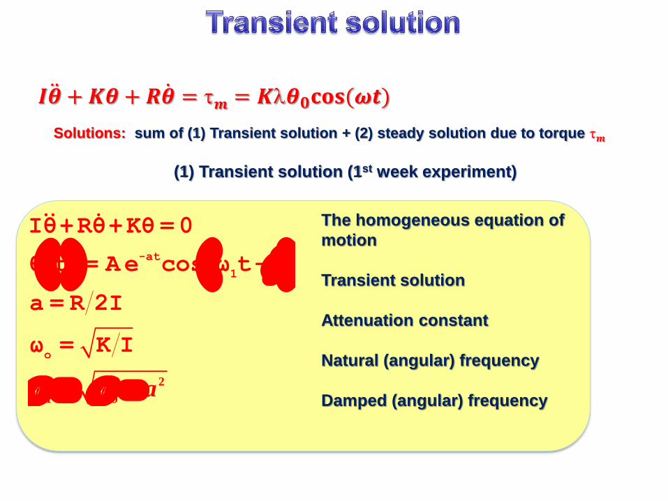
𝑰𝜽 + 𝑲𝜽 + 𝑹𝜽 = 𝒎 = 𝑲𝜽𝟎𝐜𝐨𝐬(𝝎𝒕)

𝜽𝟎𝐜𝐨𝐬(𝝎𝒕);

Angular displacement:

torque:

𝑲λ𝜽𝟎𝐜𝐨𝐬(𝝎𝒕)

Viscous damping

I is momentum of inertia, [kgm2]

R is a damping constant [N⋅m⋅s].

K is the total spring constant [Nm]

Torque by motor

𝝀 =𝑳𝟏

𝑳𝟏 + 𝑳𝟐

3/4/2013 5

Motor Pendulum

𝑰𝜽 + 𝑲𝜽 + 𝑹𝜽 = 𝒎 = 𝑲𝜽𝟎𝐜𝐨𝐬(𝝎𝒕)

Solutions: sum of (1) Transient solution + (2) steady solution due to torque 𝒎

2 2

1 oa

-at

1

o

Iθ+Rθ+Kθ=0

θ t = Ae cos ω t-

a = R 2I

ω = K I

The homogeneous equation of

motion

Transient solution

Attenuation constant

Natural (angular) frequency

Damped (angular) frequency

(1) Transient solution (1st week experiment)

3/4/2013 6

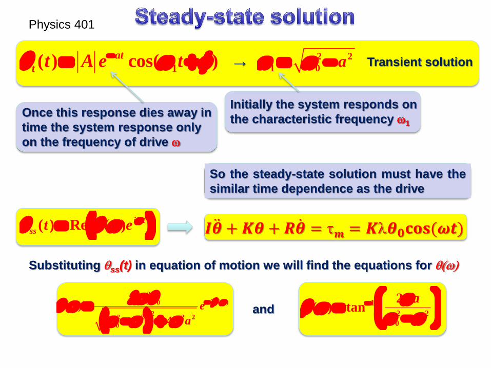
Physics 401

1( ) cos( )

at

tt A e t →

2 2

1 0a

So the steady-state solution must have the

similar time dependence as the drive

( ) Re ( )i t

sst e

Substituting ss(t) in equation of motion we will find the equations for

2

( )0 0

22 2 2 2

0

( )

4

ie

a

and

1

2 2

0

2( ) tan

a

Transient solution

Initially the system responds on

the characteristic frequency 1 Once this response dies away in

time the system response only

on the frequency of drive

𝑰𝜽 + 𝑲𝜽 + 𝑹𝜽 = 𝒎 = 𝑲𝜽𝟎𝐜𝐨𝐬(𝝎𝒕)

𝑰𝜽 + 𝑲𝜽 + 𝑹𝜽 = 𝒎 = 𝑲𝜽𝟎𝐜𝐨𝐬(𝝎𝒕)

(2) steady solution

2

22 2 2 2

2 2

cos

tan

2 22

s

o o

o

o

t B t

B

R Ra

I I

Steady state solution

Amplitude function

Phase function

Damping constant

3/4/2013 8

time domain form for steady-state solution will be

2

0 0

22 2 2 2

0

( ) cos( ( ))

4ss

t t

a

Amplitude B()

Phase

General solution for equation of motion consist of the sum of sum of

two components: (t) = t(t) + ss(t)

Coefficients A and could be determined from initial conditions

1( ) ( ) ( ) cos( ) cos( ( ))

at

t sst t t Ae t B t

0.1 1

0

1

2

(

rad

)

fd (Hz)

Fitting function:

2

0

22 2 2 2

0

( )A f

f

f f f

=2pf; =2a

-0.06 -0.04 -0.02 0.00 0.02 0.040

2

4

6

8

10

12

Count

Regular Residual of Sheet1 pend

Regular Residual of Sheet1 pend

Gauss Fit Counts

Model Gauss

Equation y=y0 + (A/(w*sqrt(PI/2)))*exp(-2*((x-xc)/w)^2)

Reduced Chi-Sqr

1.69162

Adj. R-Square 0.89685

Value Standard Error

Counts y0 1.01369 0.67924

Counts xc 6.5432E-4 0.00143

Counts w 0.02399 0.00358

Counts A 0.31875 0.05425

Counts sigma 0.01199

Counts FWHM 0.02824

Counts Height 10.60283

Model Resonance1 (User)

Equation y=A*f0^2/sqrt((f0^2-x^2)^2+x^2*gamma^2)

Reduced Chi-Sqr 3.00E-04

Adj. R-Square 0.999411988

Value Standard Error

pend A 0.286662 0.001663551

pend f0 0.500271 2.14E-04

pend gamma 0.062856 4.98E-04

f0=0.50Hz

(fitting)

To create a new fitting function

go “Tools”→”Fitting Function

Builder” or press F8

0.1 1

0

1

2

3

(

rad

)

fd (Hz)

Phase

Scanning the driving frequency we can measure the amplitude of the

pendulum oscillating and the phase shift

Both parameters Amplitude and phase can be

defined by DAQ program or using Origin

For correct representation of the resonance curve take

care about choosing of the step size in frequency.

3/4/2013 12

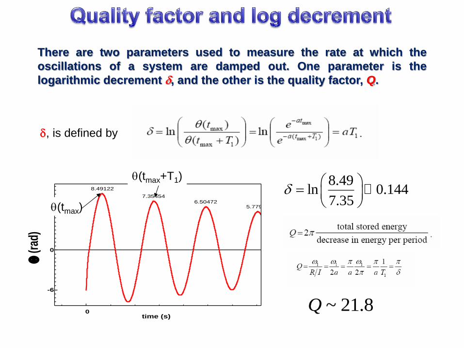
There are two parameters used to measure the rate at which the

oscillations of a system are damped out. One parameter is the

logarithmic decrement d, and the other is the quality factor, Q.

0

-6

0

6

8.49122

7.35454

6.504725.77915

5.158654.59185

4.133183.67989

3.238112.86765

2.465752.12904

1.780061.43875 1.13732 0.84893 0.57665 0.31204

time (s)

(r

ad)

(tmax)

(tmax+T1) 8.49ln 0.144

7.35d

~ 21.8Q

d, is defined by

0.3 0.4 0.5 0.6 0.7 0.8 0.9 1

0

1

2

Am

plitu

de

fd (Hz)

f=0.0626Hz

f1=0.496Hz

It can be shown that Q can

be calculated as 1/ or

f1/f. is bandwidth of the

resonance curve on the

half power level or for

amplitude graph

maxθ

2

Here Q~7.9

Consider sum of two harmonic signals of frequencies 1 and 2

y1=Asin(1t+1); y2=Bsin(2t+2)

In case A=B y=y1+y2=𝟐𝑨𝒔𝒊𝒏𝝎𝟏+𝝎𝟐

𝟐𝒕 + 𝜷𝟏 𝒄𝒐𝒔

𝝎𝟏−𝝎𝟐

𝟐𝒕 + 𝜷𝟐 ;

𝜷𝟏 =𝝋𝟏+𝝋𝟐

𝟐; 𝜷𝟐 =

𝝋𝟏−𝝋𝟐

𝟐

If 1≈2 ≈𝝎𝟏+𝝎𝟐

𝟐= and

𝝎𝟏−𝝎𝟐

𝟐 =W

y= 𝟐𝑨𝒄𝒐𝒔 W𝒕 + 𝜷𝟐 𝒔𝒊𝒏 𝒕 + 𝜷𝟏

0 5000 10000 15000

-2

0

2

y

time (s)

0.0027 0.0028 0.0029 0.003 0.0031

1

10

0.00278 0.00294

f (Hz)

1=

2=

More general case A≠B 1 and 2

y1=Asin(t); y2=Bsin((+)t)

y=y1+y2=𝑪𝒔𝒊𝒏( + )𝒕 where 𝐂 = 𝑨𝟐 + 𝑩𝟐 + 𝟐𝑨𝑩𝒄𝒐𝒔(𝒂𝒕)

𝜷 = 𝒕𝒂𝒏−𝟏𝑩sin(𝜶𝒕)

𝑨 + 𝑩cos 𝛼𝑡+

𝟎𝒊𝒇𝑨 + 𝑩𝒄𝒐𝒔(𝜶𝒕) ≥ 𝟎

𝝅𝒊𝒇𝑨 + 𝑩𝒄𝒐𝒔 𝜶𝒕 < 𝟎

0 5000 10000 15000

-2

0

2

y

time (s)

𝑨𝟐 + 𝑩𝟐 + 𝟐𝑨𝑩

𝑨𝟐 + 𝑩𝟐 − 𝟐𝑨𝑩

0.0028 0.003

0

1

10

100

0.00278 0.00294

f (Hz)

1=

2=

0 18 36 54 72

-5

0

5

(r

ad

)

t (sec)

pend

0.0 0.2 0.4 0.6 0.8 1.0 1.20

200

400

600

800

10000.42738

0.51642

Frequency (Hz)

Am

plitu

de

Two peaks

corresponding

and

Time domain trace Beating spectrum

Use Origin to analyze the frequency spectrum !

0 200 400

-4

0

4

(ra

d)

time (s)

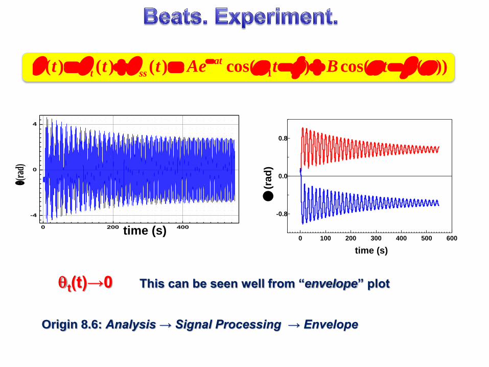
Beats dying in time.

How fast – it depends

on damping. When you

will work on resonance

data – wait until you will

see the steady state

oscillations.

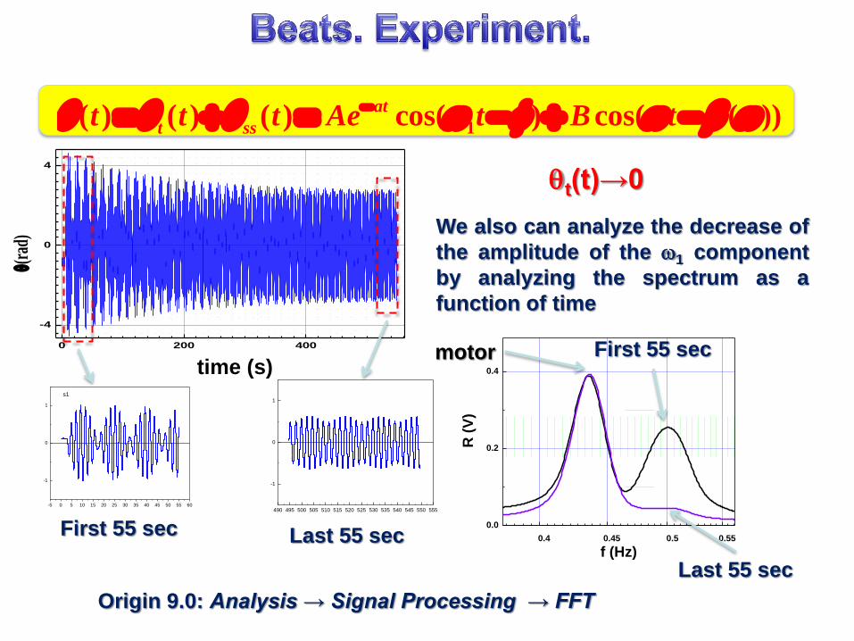
1( ) ( ) ( ) cos( ) cos( ( ))

at

t sst t t Ae t B t

t(t)→0

0 10 20 30 40 50 60

-4

0

4

time(s)

(r

ad

)

510 520 530 540 550

0

time(s)

(r

ad

)

0 200 400

-4

0

4

(ra

d)

time (s)

1( ) ( ) ( ) cos( ) cos( ( ))

at

t sst t t Ae t B t

0 100 200 300 400 500 600

-0.8

0.0

0.8

time (s)

(

rad

)

t(t)→0 This can be seen well from “envelope” plot

Origin 8.6: Analysis → Signal Processing → Envelope

1( ) ( ) ( ) cos( ) cos( ( ))

at

t sst t t Ae t B t C

First let we apply FFT

to find 1 and

Result: =3.1402rad-1 and =2.8298 rad-1

0

1( ) ( ) ( ) cos( ) cos( ( ))

t

t

t sst t t Ae t B t C

8 fitting parameters

Result from FFT: =3.1402rad-1 and =2.8298 rad-1

A 0.65012

t0 199.64912

3.13666

0.33135

B -0.74076

2.82464

-0.87829

C -0.11176

From fitting

FFT

Compare with original

pendulum spectrum Pendulum

Residuals

Possible origin of “extra” peaks:

(i) Nonlinear behavior of

pendulum

(ii) Not a single frequency driving

force provided by motor

(iii) Not ideal fitting function

0 200 400

-4

0

4

(ra

d)

time (s)

1( ) ( ) ( ) cos( ) cos( ( ))

at

t sst t t Ae t B t

t(t)→0

Origin 9.0: Analysis → Signal Processing → FFT

We also can analyze the decrease of

the amplitude of the 1 component

by analyzing the spectrum as a

function of time

-5 0 5 10 15 20 25 30 35 40 45 50 55 60

-1

0

1

s1

490 495 500 505 510 515 520 525 530 535 540 545 550 555

-1

0

1

First 55 sec Last 55 sec 0.4 0.45 0.5 0.55

0.0

0.2

0.4

R (

V)

f (Hz)

First 55 sec

Last 55 sec

motor

-5 0 5 10 15 20 25 30 35

0.0

0.4

d~0/3

time (s)

(

rad

)

0.1 1 10

10-4

10-3

10-2

10-1

Frequency (Hz)

Am

pli

tud

e

f0=0.4891Hz

fd=0.163 Hz

fd

=0.163

f0f0-fd

f0+fd

0 10 20 30

-0.3

0.0

0.3

time (s)

(

rad

)

d~0

0.1 1 10

10-4

10-3

10-2

10-1

f0

Frequency (Hz)A

mp

litu

de

f0=0.4891Hz

fd=0.244 Hz

fd

fd+f

0

In the case of driving frequency fd=f1/N where N is integer

we can observe more complicated motion of the pendulum

0.1 1 1010

2

103

104

105

106

107

0.43489

0.86796

1.30285

Frequency (Hz)

Magnitud

e

Detailed analyzes* shows that

even if ∅ = ∅𝟎 𝐬𝐢𝐧 𝝎𝒕

the driving torque contains

several harmonics of

*P. Debevec (UIUC, Department of Physics)

3/4/2013 27

R

0 10 20 30 40 50 60 70

0

1

2

3

420g step

(

rad

)

time (s)

𝝉 = 𝑹 × 𝑭

R’