Physics 370 Lab Manual

Advanced Lab

Spring 2017

Contents

1: Syllabus 5

2: Unix Tutorial 7

3: Mathematica Tutorial 11

4: Rocket Lab 15

5: Magnetopause Lab 25

6: Speed of Sound Lab 39

7: Torsion Pendulum Lab 43

3

Syllabus

Contact Information

Instructor: Jim CrumleyOffice: 107 Peter Engel Science CenterEmail: jcrumley@csbsju.edu

Phone: 363–3183Office Hour: 1:30 pm MWF days (or by appointment or just stop by)

Course Information

Lab: 12:45 – 4:45 pm T or RRoom: 112/118/146/319 Peter Engel Science CenterWeb Sites: http://www.physics.csbsju.edu/~jcrumley/370/

Canvas: https://csbsju.instructure.com/courses/6453

Experiments

Two lab assignments and three experiments will be completed by each lab group during thesemester. All groups will be doing the Rocket and Magnetopause experiments, and either thecoupled pendulum, speed of sound, or torsion pendulum experiment. The experiments will begraded based on your lab notebooks. As well as recording your data and doing the necessarycalculations, be sure to answer all of the questions from the lab in your notebook. The finalproject for this course is a formal lab report about one of your labs.

Course Schedule

Roughly half of the time there will be a lecture at 1:00 pm introducing the concepts behind alab and tools needed for a lab. You are free to work on the experiments when you like as longturn the assignments in on time, though I recommend that you do at least some of your workduring the scheduled lab periods. Note that points will be deducted for late assignments.Also, note the due dates for labs in the schedule below.

Lab Reports

Keeping a clear, complete lab notebook is an important scientific skill and much of your gradefor this class will be based on your notebooks. Refer back to your Physics 191 and 200 labmanuals for a list of what must be included in your lab notebook. Note in particular, thatyou must include a Procedure section which fleshes out what you actually did. Also, notethat though your partners and you are expected to work on the lab together, each partner

5

Syllabus

must hand in a lab notebook for each experiment. Finally, though you should discuss youranswers to the lab questions with you partner, each partner should answer the questions intheir own words.

Formal Lab Report

The formal presentation piece of this course will be a formal lab report. Specific guidelinesand topics will be provided later in the semester — see schedule below. Note that you shouldmake your first draft a complete draft, so that I can give you the most helpful feedback.

Schedule

Dates Lecture Due

1/17-19 Introduction / Unix Tutorial Pre-Survey1/24-26 Rocket Lab / Mathematica Tutorial Unix Tutorial1/31-02 Magnetopause Lab Mathematica Tutorial2/07-09 Torsion Pendulum & Speed of Sound labs —2/14-16 — —2/21-23 — —2/28-02 — 1st of 3 labs3/07-09 Spring Break —3/14-6 — —3/21-23 — —3/28-30 A few words on Formal Lab Reports 2nd of 3 labs4/04-06 Sr. thesis topics —4/11-13 — Draft of Formal Report4/18-20 Drafts returned –4/25-27 — —5/02-04 — 3rd of 3 labs5/12 — Formal Report & Thesis topic & Post Survey

Grading

The grade for this class will be based 25% on the formal lab report and 75% on the labnotebooks, tutorials, pre- and post-course surveys, and senior thesis proposals.

6

Unix Tutorial

Those who do not understand Unix are condemned to reinvent it, poorly.

Henry Spencer, University of Toronto

Unix: Some say the learning curve is steep, but you only have to climb it once.

Karl Lehenbauer

2.1 Introduction

Modern versions of Linux allow an experienced computer user to do normal computing tasksimmediately without any additional training, but to begin to harness some of the power ofLinux a little work is required. In particular, much of the power of Linux and other Unixvariants can be found in their command line interfaces (CLIs). Many current users of Microsoftand Apple operating systems have little experience with CLIs and are only used to graphicaluser interfaces (GUIs). The purpose of this exercise is to you expose to the Linux CLIs inorder to give you the experience necessary to be more productive using Linux and other Unixoperating systems in the future. Note that if you find the Unix tools that you will learn abouthere useful, there are options for available for installing them on your Microsoft Windowscomputers. MacIntosh OS X users will find that most of the tools mentioned here are alreadyinstalled on their computers (though they may not be well advertised), and the once that arenot can be downloaded fairly easily.

2.2 Account Setup

You will probably find many occasions during this lab when you will want to transfer filesback and forth between your Windows and Unix accounts. While there are many ways to dothis (including email them to yourself, put them a USB drive, or on a CD), the easiest waysinvolve transferring the files directly between the accounts involved. To get this to work takessome setup. In this section you will see how you can get direct access to your Windows filesfrom Linux, and vice-versa.

Also note that you can run a single Linux terminal window using ssh (https://sharepoint.csbsju.edu/itservices/kb/Pages/linux_ssh.asp) or a remote Linux desktop using NX(https://sharepoint.csbsju.edu/itservices/kb/Pages/misc_freenx_41.aspx) on yourown computer. You can also run some campus Windows programs using Citrix (https://sharepoint.csbsju.edu/itservices/kb/Pages/citrix_default.aspx) — you will usethis below.

7

Unix Tutorial

2.2.1 Windows File Access from Linux

1. Setup your M: drive so that it is web accessible (if you haven’t already done so) by goingto http://homedir.csbsju.edu/ .

2. Then you can access your M: Drive from Konqueror (which is both a web browser anda file manager) by opening links of the form:

webdavs://WINDOWS_USERNAME@homedir.csbsju.edu/homedir/WINDOWS_USERNAME,

where you should replace WINDOWS USERNAME with you username. When youattempt to go to that link, you should be prompted for your password. This shouldallow to to move files between your accounts using Konqueror by using Konqueror as afile manager similar to Microsoft’s Windows Explorer. You can drag and drop files, etc.

3. Once you have the link working, you should make a bookmark to your M: drive withKonqueror, so that you can easily get back there.

4. You can also get to your M: drive from other web browser like Firefox, but you youwon’t be able to drag and drop. Use the following:

https://homedir.csbsju.edu/homedir/WINDOWS USERNAME.

5. You can also use any webdavs URL, like the one for your M: drive, with other programssuch as cadaver, which is a text-mode file browser.

2.2.2 Linux File Access from Windows

While these directions are for accessing Linux files from Windows, we are going to set it upusing Citrix, a program which lets you run Windows programs from Linux.

1. Goto http://citrix.csbsju.edu/ and logon using your Windows account info. Oryou can use Citrix menu option under the CSBSJU menu on the foot menu. Cur-rently you can only use the Citrix plugin from Mozilla-based browsers (like Firefox andSeamonkey), so you can’t use Konqueror for this part. Note that you must use yourWindows username and password for Citrix.

2. Open up Windows Explorer (not Internet Explorer) from the top-level Applicationsscreen of Citrix.

3. Under the “Tools” menu of Windows Explorer, click “Map Network Drive”.

4. On the Map Network Drive Window, pick any unused letter for the Drive: choice (X:,Y:, Z:, etc.) . For the folder, put:

\\samba.csbsju.edu\YOUR UNIX USERNAME

where you should replace YOUR UNIX USERNAME with your Unix username (e.g.abstuden).

5. Your Linux directory should then show up as a drive under My Computer for WindowsExplorer whenever you startup the program. It should also be accessible from otherWindows programs.

8

Unix Tutorial

2.3 Playing with the GUI

Before we get to learning about the Linux CLI, I would like you to play around a bit with theLinux GUI. Explore the menus. Try out a few programs. Change some of the settings (maybethe wallpaper?). Then pick a game (alas, there used to be more choices) that you have neverplayed before and try it out for a few minutes. Record down the name of the game, howit works, and what score you got (if the game has a score) in your lab notebook. Or sincetheir are so few games, try another program that you have never used before, play with it,and write notes on what you have tried. Some good ones to try include gimp (Gnu ImageManipulation Program - under “Graphics” on the menu), pencil (also under “Graphics”), orAladin (under the “CSBSJU—Physics” menu.

2.4 Tutorial

The Unix tutorial at http://www.ee.surrey.ac.uk/Teaching/Unix/index.html will be the focusof this exercise. Start at the first section and work your way through the entire tutorial.Makesure that you do all of the exercises listed.

The tutorial is setup for users at another college, but all of the commands in it shouldwork here as well, though the file paths are different. Another thing to note about the tutorialis that it uses the command shell called csh. Here at CSB/SJU we use another shell, tcshwhich is based on csh, but has some more advanced features. This should not be a problembecause tcsh is more or less a superset of csh, so you should be able to do everything inthe tutorial. Note, though that there are other shells that are not as compatible with tcsh.In particular, the most commonly used shell on Linux is bash and bash has many syntaxdifferences from tcsh. If you would like to try a different shell, you can type its name at thecommand prompt. You can also change your default shell, but I wouldn’t recommend that atthis point.

To run through this tutorial you should log into one of the department’s Linux computers.Start up a web browser — Firefox, Google Chrome, Konqueror, or any other browser shouldwork fine — and go to the page mentioned above. To run the examples described in thetutorial you will also need to have a terminal window (also known as a command shell) open.There are several types that will work: xterm, konsole, gnome-terminal, and rxvt toname a few. You should be able to find them under one of the menus in the GUI.

For this exercise, you need to keep a record of the commands that you typed. I recommendthat you use the script command to do this. After you open a terminal type: script

tutorial.txt — where “tutorial.txt” is the file name that your commands will be saved in.When you are done with you session, type “exit” and it will be saved. If you have to stopthis exercise and start it up again you will want to use a different file name the second time(e.g. script tutorial2.txt, otherwise you will lose your work from the first file.

Note that for this exercise each of you should work on your own. You are free to ask forhelp from other students, but do the entire tutorial yourself.

Before you get started let me add a couple more time saving hints. In tcsh (and bash),you can scroll through previous commands that you have typed with the up and down arrowkeys. This is a big time saver if you make a typo. “Tab completion” is a related feature.When you are typing the name of a command (or file), if you hit the “Tab” key, bash willattempt to complete the command (or file) name for you.

9

Unix Tutorial

Also, Unix (or more accurately the X Windows System which provides the GUI for mostUnix systems) has several methods of copy and pasting. The Unix style way of copy andpasting is to select text using the left mouse button, then move the pointer to the place youwant to paste to, and then click the middle mouse button. Try it one or twice. Copying andpasting this way would make it quite easy to do this entire assignment without doing anytyping, but I suggest you type most of the commands given, since that will make it morelikely that you will remember them. Many programs also support the Microsoft Windowsstyle copy and pasting from their “Edit”menus (also available using Control-C, -V, and -X).Another trick with the middle mouse button involves web browsers. If you middle click on alink in most Unix browsers, the linked page will open in a new tab or window. Also, if youselect the text of an URL with the left mouse button, and you paste to a blank spot on webpage, the URL will be loaded on the browser. (You can also configure Firefox to act this wayon Windows and Mac computers.)

Also, if you get stuck while running a program from the terminal try hitting Control-C,which should exit out of the program. If that does not work, you can also try Control-Z,which suspend the program.

Another useful command is finger. Try: “finger YOUR USERNAME” and “finger jcrumley”.

2.5 Post-Test

After completing the tutorial, do the following tasks:

• Make a directory called “370” in your home directory, and put the text file(s) that youcreated recording your work on the tutorial in that directory. As part of your grade forthis tutorial I will look at those text files, so in order to enable me to do that, you willhave to change the permissions so that I can look at them. Note that you will needto add “read” and “execute” permissions for “group” for your home directory and the“370” directory. You will also have to add “read” permissions for the files that hold therecording of your session. You may want to use the “X” option to chmod (as opposedto “x”). I suggest that you keep all of your lab files in this directory, or even better insubdirectories for each lab.

• List full details about all of the files (including “hidden” files) in a directory usingls, listing the files from the newest file to the oldest. You will need to look at thedocumentation (man page) to figure this out. (Note: you should only have to use ls,sort will not be needed). Use this command to list the files in the directory “/usr/people/plasma/group_docs”. Save the command that you used and your results toa file, print the file using “enscript -r FILENAME”, and tape the results in your labnotebook.

• Type “more ∼jcrumley/public html/370/students/{$USER}” to receive a specialmessage. Write this message in your lab notebook. How does this command work?Listing the contents of that directory with “ls -l” may help you figure it out. ’

2.6 Turning in your work

Hand in your lab notebook when you are done with this exercise.

10

Mathematica Tutorial

I had a feeling once about mathematics – that I saw it all. Depth beyond depthwas revealed to me – the Byss and the Abyss. I saw – as one might see thetransit of Venus or even the Lord Mayor’s Show – a quantity passing throughinfinity and changing its sign from plus to minus. I saw exactly why it happenedand why tergiversation was inevitable – but it was after dinner and I let it go.

Winston Churchill

Anyone who cannot cope with mathematics is not fully human. At best he is atolerable subhuman who has learned to wear shoes, bathe and not make messesin the house.

Time Enough for LoveRobert Heinlein

3.1 Introduction

Computational tools beyond handled calculators are now a necessary part of any physicistsrepertoire. A wide variety of tools are available including computer codes that are written tosolve specific problems, mainstream software tools (such as spreadsheets and databases) whichcan be applied to physics problems and finally mathematical tools (such as Mathematica,Matlab, Maple, Mathcad, Sage et cetera). We will make use of tools of all of these types inthis course. The purpose of this exercise is to introduce you to one of these mathematical tools,Mathematica. Mathematica distinguishes itself from many of its competitors with its abilitiesto do exact symbolic, as well as numerical, calculations. These abilities allow Mathematicato, for example, give the solution of∫

cos(x)dx = sin(x),

while most other programs would only be able to solve problems such as∫ π/2

0cos(x)dx = 1.0.

Keep these differences in mind while doing the exercises below.In this exercise, you will first work through a Mathematica tutorial to get an idea of

Mathematica’s abilities. Then you will use Mathematica to work a more complicated physicsproblem.

11

Mathematica Tutorial

3.2 Tutorial

Start up Mathematica (this tutorial can be run on any OS that Mathematica works on).

For this tutorial you will have two choice. You can you the old-fashioned text-basedtutorial or a video screencast. It is up to you which one to try — you should get similarinformation from each.

If you want to use the text based tutorial, find and open up the “Ten Minute Tutorial” –there should be a link to it off of this lab (or the lab web site). Do not let the name fool you —it should take you much more than 10 minutes. Note that when you download Mathematicafiles you will often have to right click on them and “Save as ...”, then open them up withMathematica.

If you want to use the screencast, go to the “Hands on Start to Mathematica”

http://www.wolfram.com/broadcast/screencasts/handsonstart/. If you do the screen-cast when other people are around, please make sure that you use headphones. I will not beresponsible for any violence inflicted on you by other people if you blast this screencast in apublic lab.

As you are working through the tutorial feel free to change things in the examples. Tryout different numbers, functions, et cetera so that you have a better idea of how Mathematicaworks. Save a copy of the the tutorial in your home directory so that you can keep track ofthe changes you make while working through the tutorial.

Complete the following exercises based on the tutorial. For this exercise, you can either dothings on paper and hand-in a paper copy, or upload your results to the course Canvas site.Where appropriate print out (or save to a separate Mathematica sheet) plots and segmentsof Mathematica code showing your answers. If you decide to upload the assignment, pleaseupload the notebook (.nb) file and also a pdf copy of file. (Print the file to a pdf.)

The easiest way to answer the following questions is probably to have two Mathematicawindows open. Keep the tutorial open in one window, and do your calculations in separatewindow. In your calculations window you can copy and paste all of the questions below. Thenyou complete each calculation under the corresponding question. When you are done you canjust print the results from your window (or upload them to Canvas). Also, do not forget toinclude a written answer where one is requested.

The page numbers below refer to where you will find similar calculations in the texttutorial.

1. (p. 3) Calculate 2131 to the 31 power and 21.31 power. What is the difference betweenthese results? Why are they different? Which answer would most other mathematicaltools give? Why?

2. (p. 5) Get a numerical expression for the first 40 digits of eπ.

3. (p. 6) Expand and simplify (a+ b)(a− c)(b− d) + (d− c)(b− a)(c+ a).

4. (p. 8) Plot sinx, sinhx, and sin (sinh (x)) from 0 to 5 on the same plot. Also plot inthree dimensions the function

arctanx ln y

over the range from 0 to 5 for x and over the range from 1 to 3 for y.

12

Mathematica Tutorial

5. (p. 9) Calculated

dxarcsinh (ax) arcsinh (bx).

The compute ∫arctan (ax).

Integrate the result. Finally, numerically integrate∫ ∞−∞

e−2x2.

6. (p. 11) Solve the system of equations x2 − y2 = a and x+ 3y = b.

7. (p. 13) Solve and plot the solution to the differential equation

d2y

dx2+ y + 10 = 0,

where y(0) = 0 and y′(0) = 0.

3.3 Nonlinear Pendulum

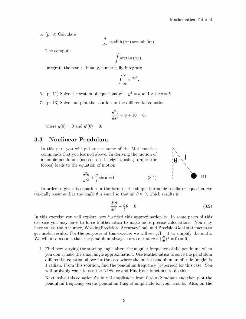
In this part you will put to use some of the Mathematicacommands that you learned above. In deriving the motion ofa simple pendulum (as seen on the right), using torques (orforces) leads to the equation of motion:

d2θ

dt2+g

lsin θ = 0 (3.1)

l

m

θ

In order to get this equation in the form of the simple harmonic oscillator equation, wetypically assume that the angle θ is small so that sin θ ≈ θ, which results in:

d2θ

dt2+g

lθ = 0 (3.2)

In this exercise you will explore how justified this approximation is. In some parts of thisexercise you may have to force Mathematica to make more precise calculations. You mayhave to use the Accuracy, WorkingPrecision, AccuracyGoal, and PrecisionGoal statements toget useful results. For the purposes of this exercise we will set g/l = 1 to simplify the math.We will also assume that the pendulum always starts out at rest (dθdt (t = 0) = 0).

1. Find how varying the starting angle alters the angular frequency of the pendulum whenyou don’t make the small angle approximation. Use Mathematica to solve the pendulumdifferential equation above for the case where the initial pendulum amplitude (angle) is1 radian. From this solution, find the pendulum frequency (1/period) for this case. Youwill probably want to use the NDSolve and FindRoot functions to do this.

Next, solve this equation for initial amplitudes from 0 to π/2 radians and then plot thependulum frequency versus pendulum (angle) amplitude for your results. Also, on the

13

Mathematica Tutorial

same figure include a plot of what the angular frequency versus amplitude is assumingthe pendulum is a simple harmonic oscillator. Take enough points so that you get afairly smooth curve. You don’t have to use Mathematica to plot your results — anyplotting program is fine.

2. Calculate at what amplitude the angular frequency differs from the ideal angular fre-quency by 10 % ? By 1 % ? By 0.01 % ? By 0.0001 % ? What does this tell youabout the accuracy of the small angle approximation? Under what conditions is thisapproximation valid?

3. One of the applications of pendulums is in clocks. Calculate how long it would takefor a clock using this pendulum to be displaying a time that is off by a minute if theamplitude of the pendulum is 0.1◦? 1◦? 10◦? 30◦? 90◦?

14

Rocket Lab

A Severe Strain on the CredulityAs a method of sending a missile to the higher, and even to the highest parts ofthe earth’s atmospheric envelope, Professor Goddard’s rocket is a practicable andtherefore promising device. It is when one considers the multiple-charge rocketas a traveler to the moon that one begins to doubt . . . for after the rocket quitsour air and really starts on its journey, its flight would be neither accelerated normaintained by the explosion of the charges it then might have left. ProfessorGoddard, with his “chair” in Clark College and countenancing of theSmithsonian Institution, does not know the relation of action to re-action, and ofthe need to have something better than a vacuum against which to react . . . Ofcourse he only seems to lack the knowledge ladled out daily in high schools.

New York Times Editorial, 1920Concerning Robert Goddard, rocketry pioneer

4.1 Introduction

The problem of the flight of a rocket is an interesting problem for both practical and more the-oretical reasons. The flight of a rocket can be pursued at several different levels theoretically.The simplest level is a basic constant force problem using Newton’s Laws:∑

~F = m~a. (4.1)

At this simple level we would only deal with two forces — gravity and rocket thrust. In thecase of vertical flight this leads to:

T −mg = ma = mdv

dt= m

d2y

dt2(4.2)

where T is the thrust. Assuming constant thrust, solution of this differential equation istrivial:

a =T

m− g (4.3)

v = v0 + at = v0 +

(T

m− g)t (4.4)

y = y0 +1

2at2 = y0 +

1

2

(T

m− g)t2. (4.5)

15

Rocket Lab

This solution is appropriate in cases such as in when the rocket’s mass is almost constant andair resistance is negligible, but neither of these conditions will hold for this lab.

In order to analyze our model rockets we will have to deal with at least three complicatingfactors. In our rocket engines, thrust as a function of time will be much closer parabolic thanconstant, so we will have to deal with varying the thrust. Next, the mass of the rocket willchange as it burns off its propellant, so we will not be able to use a constant mass in ourequations. Finally, the air resistance will add another force to our equation of motion.

4.1.1 Time-Varying Thrust

The simplest time-varying thrust that we can consider is essentially a square wave — therocket engine is on at some constant value until it burns out. While this is not a goodapproximation to our rocket, it is a useful case to consider because it shows some featuresthat will also appear in our more realistic thrust curves. The on/off character of this typeof thrust curve leads to the technique of splitting the problem in two. First, solve for therocket’s motion for the case of constant thrust, using the equations 4.3–4.5. Then after therocket engine quits, start with initial conditions based on when the engine stopped and solveusing the same equations with a thrust of 0.

In order to deal with thrust curves that are more realistic than square waves, we needto come up with expressions for thrust as a function of time: T → T (t). We will find thethrust curves in two ways: by using the manufacturer’s published curves (Section 4.2.2) andexperimentally using a force meter (Section 4.2.3).

4.1.2 Time-Varying Mass

Since we will not be able to directly measure how the mass of the rocket engine changes duringthe rocket’s flight, we a need a proxy that will allow us to deal with mass as a function oftime (m → m(t)). The obvious choice is to assume that for each unit of mass that is lost aconstant amount of thrust is derived:

− dme

dt∝ T. (4.6)

ordme

dt= −αT (t), (4.7)

where α is a proportionality constant. With this idea we can use the initial (mei) and final(mef ) mass of the rocket engine along with our thrust curve to get me(t). Solving thisdifferential equation we get:

me(t) = mei − α∫ t

0T (t′)dt′ (4.8)

or after the engine is exhausted:

α =mei −mef∫T (t)dt

(4.9)

The quantity∫T (t)dt is known as the impulse, and it is provided by the engine manu-

facturer, though it also can be calculated directly from the thrust function. So we can find αusing the equation 4.9 and then use it in the equation 4.8 for the time varying mass, me(t).

16

Rocket Lab

4.1.3 Air resistance

Air resistance is a complicated subject and for most real problems it cannot be dealt withanalytically. Typically one of a variety of approximations is applied depending upon whichfluid regime the problem falls under [Marion and Thorton, 1995]. For this lab we will use :

f(t) = −bv(t)2 (4.10)

where here “−” means that the drag force is in the opposite direction from the direction thatthe rocket moves and b is the drag constant. Other common forms for the drag force dependon the speed to the first power. The constant b depends on the fluid the rocket is movingthrough and the shape of the rocket:

b =1

2ρcdA (4.11)

where ρ is the density of air, cd is the drag coefficient, and A is the surface area of the cross-section of the rocket. We will measure the cross-sectional area, and the density of air can bedetermined from the ideal gas law and the weather conditions at the time of the flight of therocket. The drag coefficient depends on the shape of the rocket and the smoothness of itssurface. The drag coefficient is one of the major unknown quantities that we will determinein this lab. Values for this quantity should end up being somewhere between 0.2 and 2.

Since the form for the drag force law changes as the speed of an object changes, the dragcoefficient is not constant over wide speed ranges. In this lab we will first use one type ofrocket engine to determine the drag coefficient. With another type of rocket engine we willthen use the drag coefficient as a known value, and predict the maximum height of the rocket.

4.1.4 Combined Equation

Finally, we get to an equation including time-varying thrust, time-varying mass, and airresistance

a(t) =T (t)

m(t)− g − bv(t)2

m(t)(4.12)

This is the equation that we will solve to find the drag coefficient for the rocket.

4.2 Experimental Procedure

4.2.1 Building your Rocket

Follow the instructions included with the rockets for putting your rocket together. Put youparachute together, but do not attach the nose cone or parachute to the shock. You willattach the cargo section to the shock cord when you are going to launch. Sand and paint yourrockets in order to have a smooth surface that minimizes drag.

1. Does painting your rocket cause have any positive or negative effects on the range ofthe rocket? If so, try to estimate these effects.

17

Rocket Lab

4.2.2 Finding Thrust Function from Manufacturer’s Thrust Curves

In order to use the manufacturer’s thrust curves in data analysis, the curves must be convertedinto a numerical form. To do this we will convert the continuous curve into discrete thrustversus time values using a computer program available in room 118 PE. The program allowsyou to calibrate and then trace out a graph in order to convert the plot into data points. Usethis program to get thrust function data for both types of engines that will be used in thislab.

To use this program log into the Unix dummy terminal next to the digitizing board.(After logging in, you may have to enter the terminal type which is “vt100”.) Tape yourthrust plot to the board so that it won’t move while you are taking data. The program touse is called “digitizer.” Start the program by typing its name. Hit the “0” button on thecursor/mouse whenever you need to mark a location. For each axis in turn, choose a linearscale and then calibrate the digitizing board by choosing minimum and maximum locationsand enter the numerical values for those locations. Then the program will have enter youa name and comment for your data file. You will then trace out the thrust curve with thecursor, taking data points at intervals that you find appropriate. More points should be takenwhen the graph is curved, fewer when its straight. For the sake of this program, you will nothave to determine error bars. When you are done collecting data, press “Control-D” to stopthe program. You should then plot your data using a program of your choosing to check thatyour curves match the manufacturers curves. Include these plots in your lab notebook.

1. If we could assume that the manufacturer’s thrust curves were free of error, we wouldstill have uncertainty in our thrust versus time values because of the method that weare using to obtain our data from the curves. What factors limit our ability to convertthe curves into numerical data?

2. Estimate the uncertainty due to these limitations. How does this uncertainty compareto the variations between engines due to the manufacturing process? You may be betterable to answer these questions after firing some of the engines.

4.2.3 Experimental Determination of Thrust Curves

Thrust curves will be determined using a force meter connected to a computer. Make surethat the interface is set to take data at a rate of at least 100 samples per second. See thepictures on the web for one possible way to set up this equipment. The equipment should besetup under a hood to minimize the smoke dispersal through the building. Calibrate the forcemeter with known masses. Have your instructor check your setup before firing the rocketengines.

The Vernier Froce Sensor, LabQuest Mini sensor interface, and Logger Pro software. Whenyou plug connect the LabQuest Mini to the computer its LED will initially be red. If theinterface is getting enough power, the LED will turn amber. Then, when you start LoggerPro,it should turn green. If it does not turn green, the sensor will not work. Not that if you areusing a USB extension cable, you may also need to use a powered USB hub.

The Labquest Mini interface should be connect to the computer named yalow. You shouldrun Logger Pro on that computer. You can log into yalow using ssh:

ssh -Y yalow.physics.csbsju.edu

Note that the “.physics.csbsju.edu” won’t be needed from campus Linux machines.

18

Rocket Lab

Once logged into yalow, you can start LoggerPro by typing: loggerpro& at the commandprompt, or by finding LoggerPro on the menus if you are logged in directly at yalow.

Once you have your engine ready to be fired and LoggerPro started, you should zero outthe sensor by hitting the blue 0 with a slash through it button. You can then collect data byhitting the green arrow button, and stop data collection by hitting the red button.

Verify the thrust curve by firing three engines of a given type. Plot your three data curves.Include these plots in your lab notebook. Also, be sure to save a file of your data and exportyour data into a form that is usable by other programs (csv or txt files work best). You shouldthen transfer your data from yalow, to the campus Linux computers. One way to transfer thisdata is to run the makeyalow command on one of the regular campus Linux computers. Thiscommand will make a directory called 2yalow in whatever directory you run it from. Thisdirectory will link to directory called “/backup/$USER” (where $USER is replaced by yourusername), so if you copy your thrust to “/backup/$USER” on yalow, they will be visibleunder 2yalow on the other Linux computers.

Finally, please clean the fume hood when you are done with your rocket firings.

1. How much variation is there between the curves from the three trials? How much ofthis variation do you think is due to the instruments used to measure the thrust curvesand how much is due to intrinsic variations in the rocket engines?

2. How well do your thrust curves compare to the manufacturer’s curves? Are the differ-ences between them systematic or random?

Based on your results in this section and the previous section, decide whether you aregoing to use the data from the manufacturer’s thrust curves or your experimental data tomodel the thrust of the rockets. Justify your decision. If you decide to use your experimentaldata, then you should come up with an experimental thrust curve that combines your trialsand an estimate of the uncertainty for it.

4.2.4 Rocket Launches

At least four people will be needed to complete the rocket launches, so you will need tocoordinate with other groups to schedule your launches. If no one in your groups has donea launch previously, then your instructor will want to go with to help you set up. Note thatyou will want to record the temperatures and pressure for the dates of your launches so thatyou can calculate the air density.

Equipment Checklist

• Your rocket and parachute

• Cargo section and nose cone

• Altimeter with battery

• Laptop with cable for altimeter (optional)

• Four A and four B engines

• Igniters

19

Rocket Lab

• Recovery wadding

• Launch pad

• launcher with key

• Two tripods with angle measuring devices

• 300 foot measuring tape

• stop watches

Rocket engines are described by names such as A8-3. The letter in the name stands for thetotal impulse of the rocket, with A engines having total impulse of up to 2.5 N · s, with eachsubsequent letter having up to twice the total impulse (B has 5 N · s, etc.). The first numberin the name is the rockets average thrust in N. Finally, the last number is the delay time inseconds between the burnout of the rocket and the ejection of the parachute. In practice, thisdelay time seems to vary quite a bit from the published values.

Do three rocket launches with A engines and use this data to determine the drag coefficientof your rocket. If any of the three launches seem to be much higher or lower than the others, doa fourth launch. Also, do three launches with B engines and compare this data to predictionsbased on the drag coefficient from the A engine launches.

Several measurements will be needed for each rocket launch including the apogee (maxi-mum altitude) of the rocket, the flight time till apogee and the initial and final mass of therocket engine. Note that you will also need the total mass of the loaded rocket for the calcu-lations — the engine masses are just used to find how the rocket mass changes. As describedabove, you will also need to determine the cross-sectional area of the rocket. Finally, youwill need some weather conditions for each time that you launch, in order to determine thedensity of air. The name of individual measuring each piece of data should be recorded aswell as the data itself in order to aid in the isolation of any systematic error.

4.2.4.1 Apogee Time

While doing rocket launches, anyone (including the rocket launcher) not making angle mea-surements for the geometrical apogee determination should measure the time to apogee. Timeto apogee can be difficult to determine, so having several people measure it and taking a meanis advantageous.

These rockets have an explosive charge which will deploy their parachutes. The secondnumber on the rocket engine name is the number of seconds until the charge is supposed todetonate, but for real rockets the time till the charge varies wildly from this number. Duringa flight, depending on the engine and the mass of the rocket and the performance of theengine, the apogee will happen two different ways. Either the rocket’s motion will turn overbefore the parachute pops out, or the apogee will occur when the parachute pops out. If themotion turns over, determine the apogee based on when the rocket is at its highest height. Ifthe parachute comes out first, mark the apogee time as when the parachute comes out sincethe rocket’s upward motion will be halted by the parachute. You should keep this behaviorin mind when comparing your experimental results to the theoretical calculations, since thetheoretical calculations do not account for the possibility of the parachute coming out early.

20

Rocket Lab

4.2.4.2 Apogee Determination

Two methods will be used to the determine the maximum altitude of the rocket: geometricaland electronic. The geometrical method relies on multiple observers determining the angle therocket makes with respect to the horizontal at its maximum height. The electronic methodrelies on an altimeter that measures pressure changes that occur as the rocket rises in orderto find its altitude.

4.2.4.2.1 Electronic Apogee Determination

For the electronic method we will be using PerfectFlite Pnut manual [Perfect Flite, 2012c]and/or APRA manual [Perfect Flite, 2012a] altimeters. (See the links in the previous sectionfor more details on the altimeters. Note that the altimeter may not function properly whenthe temperature is much below 0 ◦C. The altimeter reports the apogee altitude as a seriesof beeps after the flight. The Pnut altimeter can also store flight profile information (heightversus time), which can be retrieved by attaching it to a computer. Keep track of the orderof your (and other groups) flights, so that the data can be matched up with the correct flight.Detailed instructions for using the data retrieval program are included in the DT3U manual[Perfect Flite, 2012b].

In order to use the altimeter you will have to install the payload section on your rocketand include the altimeter inside the payload section. Make sure to secure the payload andaltimeter section to the rest of your rocket, so that it all descends as one piece. After theflight connect the altimeter to the computer using the Serial/USB cable and extract the data.Be sure to save the data with a name that you will be able to remember later on.

4.2.4.2.2 Geometrical Apogee Determination

The simple method of geometrically determining the apogee of the rocket only requiresthe determination of one angle and one distance. An observer measures their distance fromthe launch site and then measures the angle the rocket is above the horizontal at its apogee.In this case the altitude is

h = x tan θ. (4.13)

This method’s accuracy is limited by the need for the rocket’s launch to be perfectly vertical,but it is still a good first approximation to finding the altitude. For each flight you shoulduse this method, as well as the one described below to determine the altitude. Note that thismethod gives the most accurate results when θ is near 45◦.

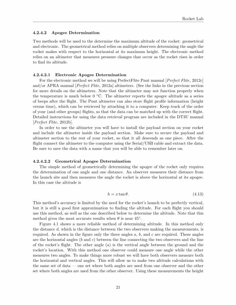
Figure 4.1 shows a more reliable method of determining altitude. In this method onlythe distance d, which is the distance between the two observers making the measurements, isrequired. As shown in the figure only the three angles a, b, and c are required. These anglesare the horizontal angles (b and c) between the line connecting the two observers and the lineof the rocket’s flight. The other angle (a) is the vertical angle between the ground and therocket’s location. With this method one observer could measure one angle while the othermeasures two angles. To make things more robust we will have both observers measure boththe horizontal and vertical angles. This will allow us to make two altitude calculations withthe same set of data — one set where both angles are used from one observer and the otherset where both angles are used from the other observer. Using these measurements the height

21

Rocket Lab

Figure 4.1: The figure above shows how to determine the altitude of the rocket usingmeasurements from two observers. This figure is adapted from http://www.grc.nasa.gov/.

of the rocket is

h =d tan a sin c

sin (b+ c)(4.14)

[Benson, 2003]. Beware that this formula assumes that all angles are less than 90 degrees.If your angles are larger, then you have probably made a mistake. When deciding where tolocate the observers for your launches, note that this method also gives the best results whenthe angles are near 45◦. For this reason, you probably want to set up your observers so thattheir locations make a equilateral right triangle, with the launching pad at the right angle.In order to get angles near 45◦ for the vertical angles, you will also want the distances fromthe observers to the launch pad to be roughly the same as the expected maximum altitude ofthe rocket. Typical apogees for the experiment are roughly 40 m for A engines and 100 m forB engines.

Note that you should end up with four geometrical estimates of the apogee height for eachlaunch — two from the simple one-angle method and two from the multi-angle method.

4.3 Data Analysis

4.3.1 Using Mathematica

We will use Mathematica to solve our version of the rocket equation (equation 4.12). Whileperforming this analysis you can refer to the sample file performing this calculation in asimplified case.

The first step in this calculation is to enter your thrust data. Those groups that determinedthe thrust curve experimentally should use evaluate their two types of thrust data, and usewhichever type they find appropriate here. Be sure to justify your choice. Note that whichwhichever type of data you use. you need to have your thrust curve defined from 0 up untilroughly 5 or 10 seconds. You may want to extend your thrust curve by putting in thrusts of

22

Rocket Lab

N for times greater than 1 second in your thrust curve files. In other other, add ordered pairslike “1 0” . . . “10 0” to your files.

In order for Mathematica to be able to use this data you must enter the data into a table.To do this you will likely want to use the Import or ReadList function. Something along thelines of

table1 = Import[“/home/f13/abstuden/A8 thrust data′′]

or

table1 = ReadList[“/home/f13/abstuden/A8 thrust data′′, {Number, Number, Number, Number}]

should work. The first parameter is the path to the data file, while the other parameterscorrespond to the columns in your data file. You may need to edit your file to get it into aform that Mathematica can deal with. In particular, you may want to use a text editor toremove the header lines from the data file. Once you have your data table, you will probablywant to use the Interpolation function to make the data into a continuous function. Besure to graph your thrust curve over the full time range that you want do calculations overto be sure that it looks reasonable. Mathematica sometimes puts spikes and other unphysicalfeatures into Interpolating Functions. If you have problems of this sort, you may have to altersome of the options to Interpolation. For each engine, calculate the total impulse of theengine and compare it to the expected value.

For the A engine data, consider the drag coefficient, cd to be an unknown and solve for itby trial and error for each of the three launches that you did with the A engines. To find cdvary it until your y(t) plot matches your measurements of the rocket flight. Find the meanand standard deviation for the drag coefficient.

For the B engines, use the drag coefficient that you determined above to find a predictedapogee (including uncertainty) for the B engine flights. Also, re-calculate the drag coefficientusing your B engine apogee data as the known quantities.

Include a printout of one version of A engine Mathematica analysis and one version ofyour B engine Mathematica analysis in your lab notebook.

1. Compare the prediction of the B engine apogee with your experimental determinationsof the apogee. Do they agree? Why or why not?

2. Compare the estimates of the drag coefficient that got for the A engines with the estimateform the B engines. Do they agree? If not, how could you explain the discrepancy?

4.4 Conclusion

As well as answering the questions listed above, comment on your results.

1. Describe in more detail than is presented here how the electronic altimeter works.

2. Explain how the geometrical method of determining altitude using two observers im-proves accuracy. Hint: there is more to it than simply having better statistics to averageover.

3. Do your results support the idea of the drag coefficient being a true constant for thespeed regime your rockets were tested in? Why or why not? Make sure to use theuncertainties that you obtained for the drag coefficients in defending your answer.

23

Rocket Lab

4.5 Bibliography

Benson, T., A beginner’s guide to model rockets, http://www.grc.nasa.gov/WWW/K-12/airplane/rkthowhi.html, 2003.

Marion, J. B., and S. T. Thorton, Classical Dynamics of Particle and Systems, Thomson,Brooks/Cole, Pacific Grove, California, 1995.

Perfect Flite, APRA Users Manual, http://perfectflite.com/APRA manual.pdf, 2012a.

Perfect Flite, DT3U Users Manual, http://perfectflite.com/DT3U manual.pdf, 2012b.

Perfect Flite, Pnut Users Manual, http://perfectflite.com/Pnut manual.pdf, 2012c.

24

Magnetopause Lab

Space is big. You just won’t believe how vastly, hugely, mind-bogglingly big it is.I mean, you may think it’s a long way down the road to the drug store, butthat’s just peanuts to space.

Douglas Adams, The Hitchhiker’s Guide to the Galaxy

It is contrary to reasoning to say that there is a vacuum or space in which thereis absolutely nothing.

Descartes

5.1 Introduction

Though outer space is often described as a vacuum, in actuality there are particles everywherein the solar system, and there is continuous activity in the region between the celestial bodies.The study of this part of the solar system is called Space Physics [Kivelson et al., 1995], orsometimes Plasma Space Physics after the particles that fill this region. A plasma is a ionizedgas, where some of the electrons have been stripped off of atoms creating a mixtures of freeelectrons and positively charged ions.

Most of the plasma particles filling the solar system can trace their origin to the solarwind, which comes from the outer region of the sun’s atmosphere continually being blown offof the sun. The solar wind typically has a speed of about 400 km/s, though it can range upto about 1200 km/s.

5.1.1 The Magnetosphere

When the solar wind reaches the earth, it interacts with the earth’s magnetic field to form aregion known as the magnetosphere (See Figure 5.1). The earth’s magnetosphere is the regionof space where the earth’s magnetic field dominates behavior of the plasma, just as the sun’smagnetic field does in the solar wind. The magnetosphere has many regions, though only afew will be of interest to us in this lab.

The first region of interest (though it is not technically part of the magnetosphere) isknown as the bow shock. The bow shock is caused by the solar wind meeting an obstructionits flow in the form of the earth. The solar wind has to flow around the the earth, and indoing a shock formed. The bow shock gets its name from the fact that the physics behindthe creation of this shock are similar to the shock formed by the bow of a boat as the boatmoves through the water.

25

Magnetopause Lab

Magnetosheath

Magnetopause

Solar wind

Bow shock Earth

Magnetosphere

Figure 5.1: This figure shows the basic structure of the magnetosphere.

Nearer to the earth is the magnetopause. The magnetopause marks the furthest that theearth’s magnetic field extends, which makes the magnetopause the boundary of the magne-tosphere. The magnetosheath is the region of space between the bow shock and the magne-topause.

Nearer still to the earth are the ring currents and radiation belts (also known as the VanAllen belts). These areas are located within a few RE of the earth above the equator and lowlatitudes. The relatively high number of high energy particles in these areas make this regiondangerous for spacecraft and difficult to observe.

5.1.2 Solar Activity

The surface of the sun, and consequently the solar wind, experiences a variety of events,including flares and coronal mass ejections (CMEs). These events can change both the speedand the number density (particles per volume) of the plasma in the solar wind. When thesolar wind from one of these events reaches the earth, the events are called Solar Storms orMagnetic Storms. These variations in the solar wind cause the location of the both the bowshock and the magnetopause vary. Studying the variation in the distance from the earth tothe magnetopause is one of the aims of this lab.

The location of the magnetopause is important because the magnetosphere shields theearth and most satellites that go around the earth from the direct effects of the solar wind.When the magnetopause moves, some satellite that are typically protected by the magne-tosphere can find themselves in the solar wind. In particular, many satellites are placed ingeosynchronous orbits so that they are always above a fixed location on the earth. Geosyn-chronous orbits are roughly 42000 km (or 6.6 RE , where 1 RE equals the radius of the earth)from the center of the earth. During normal solar wind conditions the standoff distance of themagnetopause (the distance from the center of the earth to the point of the magnetopausethat is on the line between the sun and the earth) is roughly 10 RE . During extremely strongSolar Storms the magnetopause can move in closer than geosynchronous orbit. This exposesmany satellites to direct contact with extreme solar wind conditions, and satellites are oftendamaged or lost when this happens.

26

Magnetopause Lab

5.2 Theory

5.2.1 Magnetopause Location

The location of the magnetopause along the line between the earth and the sun can be derivedby balancing the magnetic pressure of the magnetosphere with the dynamic pressure of thesolar wind (see Figure 5.2. The equation for this balance takes the form:

ro(RE) = 107.4(nswv2sw)−

16 (5.1)

where ro is the standoff distance from the earth to the magnetopause along the line to thesun measured in RE , nsw is the number density of the plasma in the solar wind in cm−3,and vsw is the speed of the solar wind in km/s [Kivelson et al., 1995, pages 173-4]. Theentire magnetopause boundary has also been fit to various empirical functions by a numberof researchers. We will use expressions from a set of models for the earth’s magnetopauseposition for normal solar wind conditions[Shue et al., 1997] and extreme events[Shue et al.,1998]. The expressions we will use are

r = ro

( 2

1 + cos θ

)α(5.2)

ro = (10.22 + 1.29 tanh [0.184(Bz + 8.14)])(Dp)−16.6 (5.3)

α = (0.58− 0.007Bz)[1 + 0.024 ln (Dp)] (5.4)

where r is the distance from the earth to the magnetopause boundary, ro is the magnetospherestandoff distance, Bz is the z-component of the solar wind’s magnetic field, Dp is the dynamicpressure of the solar wind, and α is the amount of tail flaring from the night side of themagnetopause.

5.2.2 Coordinate Systems

A variety of different coordinate systems are used to measure locations in space, and in thislab you will have to use data in several of these coordinate systems. More information onthese coordinate systems can be found in books [Kivelson et al., 1995] or online [ESA, 2005].

5.2.2.1 Geocentric Solar Ecliptic

The geocentric solar ecliptic (GSE) coordinate system has its x-axis point from the earth tothe sun and its y-axis is in the ecliptic plane (the plane of the earth’s orbit) pointing in thedirection of dusk (opposite the direction of the earth’s orbital motion). Its z-axis is in thedirection of the ecliptic pole.

5.2.2.2 Geocentric Solar Magnetospheric

In geocentric solar magnetospheric (GSM) coordinates, as in GSE coordinates, the x-axispoints from the earth to the sun. Its z-axis points in the direction of the north magnetic pole.Its y-axis, is perpendicular to the other two, so that a right-handed coordinate system results.The difference between the this system and the GSE system is a simple rotation about thex-axis.

27

Magnetopause Lab

EB

Magnetopause

Solar wind

Magnetosphere

θ

positive ions

electrons

Current

Figure 5.2: The pressure balance at the magnetopause between the solar wind dynamicpressure and Earth’s magnetic pressure. The electrons deflect counter-clockwise and thepositive ions deflect clockwise when reflecting at the magnetopause.

5.2.2.3 Geocentric Equatorial Inertial

In geocentric equatorial inertial (GEI) coordinates (also known as geocentric solar inertial(GCI)), the x-axis points from the earth to the the first point of Aries (the location of thesun at vernal equinox). This line is where the equatorial and ecliptic planes intersect. Thez-axis is parallel to the earth’s rotation axis, and the y-axis complete the the right-handedcoordinate system.

5.3 Simulation

In this portion of the lab you will use a computer simulation to model the location ofthe magnetopause. The model we will use is called BATS-R-US [Hansen et al., 2002], theBlock-Adaptive-Tree-Solarwind-Roe-Upwind-Scheme, which was developed at the Universityof Michigan. We will be running the simulations on super-computers at NASA-Goddard runby the Community Coordinate Modeling Center (CCMC) [NASA, 2005].

This code is a magnetohydrodynamics (MHD) simulation. In MHD, a plasma is approxi-mated as a quasi-neutral fluid, and that fluid is assumed to be governed by equations that aregeneralizations of the equations of fluid dynamics. MHD simulations ignore the behavior andphysics of individual particles, and deal with the collective behavior of the plasma as a fluid.For this reason, MHD simulations work well on large scales, but miss much of the smallerscale physics.

5.3.1 BATS-R-US Input File

To use BATS-R-US, you must first create an input file which tells the simulation the typeof conditions that you would like to simulate. The input file is a simple text file with the

28

Magnetopause Lab

Year M D Hr Mn s ms Bx By Bz Vx Vy Vz n TnT km/s cm−3 K

2000 1 1 0 0 0 0 5 0.0001 0.0001 -500 0 0 10 2000002000 1 1 0 5 0 0 5 0.0001 0.0001 -500 0 0 10 2000002000 1 1 0 10 0 0 5 0.0001 0.0001 -500 0 0 10 2000002000 1 1 0 15 0 0 5 0.0001 0.0001 -500 0 0 10 2000002000 1 1 0 20 0 0 5 0.0001 0.0001 -1000 0 0 10 2000002000 1 1 0 25 0 0 5 0.0001 0.0001 -1000 0 0 10 2000002000 1 1 0 30 0 0 5 0.0001 0.0001 -1000 0 0 10 2000002000 1 1 0 35 0 0 5 0.0001 0.0001 -1200 0 0 10 2000002000 1 1 0 40 0 0 5 0.0001 0.0001 -1200 0 0 10 2000002000 1 1 0 45 0 0 5 0.0001 0.0001 -1200 0 0 10 200000

Table 5.1: Sample BATRUS input file segment

conditions at different times listed. A sample input file is available (batrus input template.txt)and Table 5.1 includes a portion of one.

First, note that the first two lines are a header line which should not be included whenyou try to run the simulation. Next, note that the first 7 columns of the input file set thetime for the conditions that follow. Since we will not be simulating real conditions from areal day, the date we pick is arbitrary, though the usual convention is to pick 1/1/2000 forthe date. The time differences are significant, though for our work here we will just use a 5minute time difference between each of the points that we use. The next six columns give thethree components of the solar wind magnetic field in nT, followed by the three componentsof the solar wind speed in km/s. Note that Vx must be negative, so that the solar wind ismoving the earth and that the simulation adds the extra constraint that the magnitude of Vx

must be 200 km/s or greater. Also note that the components of B must not b 0. The finaltwo columns are the solar wind plasma number density in cm−3 and the solar wind plasmatemperature in Kelvin.

In this lab you will complete one simulation run where you vary, in turn, two parameters.In one part of the run you will vary Vx and in the other part you will vary n. For each run youwill compare the location of the subsolar point of the magnetopause to the location predictedby equation 5.1. Ask your instructor what specific range you should use for each. Note thatbecause of the way the simulation interpolates the parameters between input lines that youwill always want to have consecutive lines that have the same parameter values. If there areplaces where you have large jumps in input parameters (typically when you go from constantVx to constant n), you should have four lines in a row with the same values in order to givethe simulation more time to settle down to an equilibrium For most simulations, there will betwo places where you need to do this - at the beginning of the simulation and in the middle.Before submitting your simulation, have your instructor check your input parameters.

Make sure to save your input parameters in your lab notebook. Include either your inputtxt file or the graph of conditions, or preferably both.

29

Magnetopause Lab

-1400-1200

-1000

-800

-600

-400-200

N (

cm

-3)

0.0 0.5 1.0 1.5 2.0Time (hours)

5

10

15

20

Vx (

km

/s)

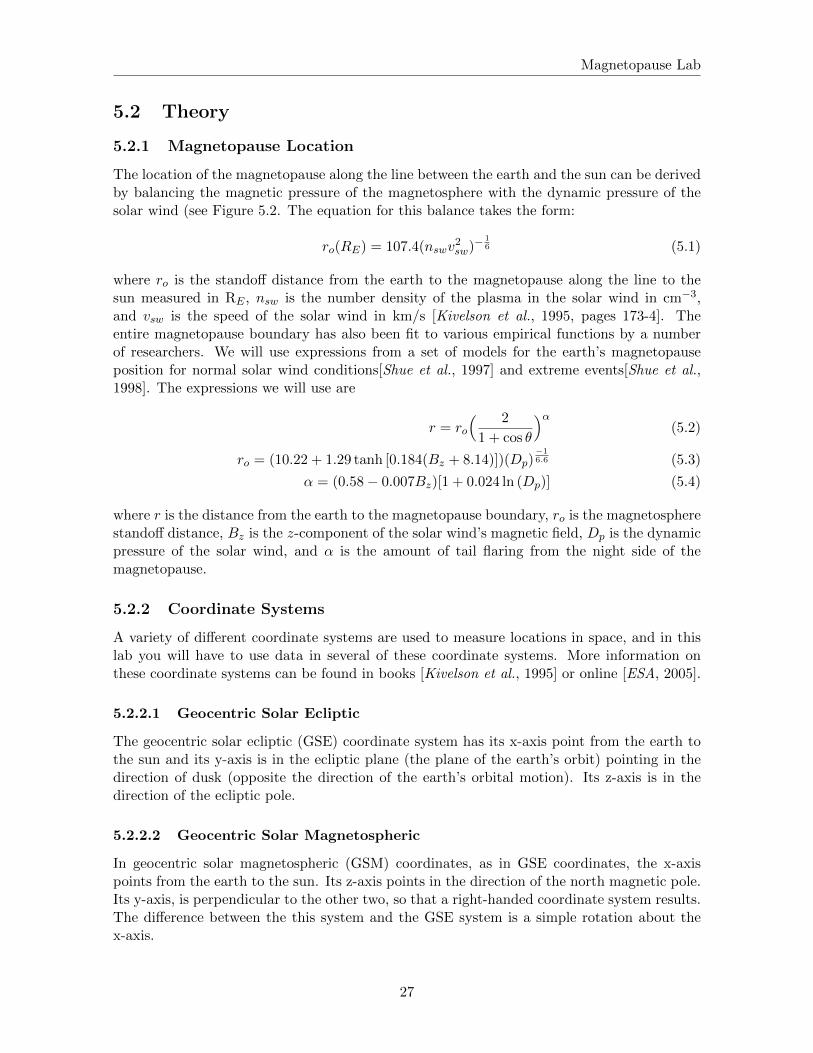
Figure 5.3: An excerpt of the interesting part of the solar wind conditions to input for thesimulation. Note that in this case the solar wind number density (upper plot) is held constantfor the first half and varied for the second half of the simulation, while the solar wind speed(lower plot) is held constant for the first half and varied for the second half of the simulation.Also note that the step pattern is used in the solar wind conditions to allow the magnetopauselocation to come to equilibrium after the conditions are varied.

5.3.2 Submitting Your BAT-R-US Simulation Run

As stated explained above, we will be running the BAT-R-US simulation using supercomputersat CCMC. This section describes how to submit your simulation run.

1. Go to http://ccmc.gsfc.nasa.gov/.

2. Click on “Request a Model Run” on the top.

3. In the “Magnetosphere” section, go to the “BATSRUS” line. Open “Magnetosphererun instructions” link in a new browser tab or window. Then click on the “Request aRun” link as well.

4. Fill in all required areas about yourself. Pick a title for your run — something like“Magnetopause location under various solar wind conditions” and add the key word“educational” to the appropriate boxes. Choose “BATSRUS version 20140611: withoutRCM and without RBE” for the simulation.

5. Also choose “Run Type: Model” and fill in the ending time for your simulation i( thelength of your run) and then hit the “Submit” button

6. On the next page, under “Solar Wind Input”, click “Upload file” button and then clickbrowse to find the file in your directories. Making sure that you input data looks likethe data above, except that your file should have with no header lines at the top. Hitthe “Browse” button to find the file. After you have found your file, also input a valuefor the “Fixed X Component of SW Magnetic Field” — that value will be 5.

30

Magnetopause Lab

7. Under “Magnetosphere Grid”, leave the simulation grid at 1,007,616 cells. Under “Iono-sphere Conductance Model:” leave the value in the “Auroral Conductances driven bysolar irradiance and field-aligned electric currents F10.7 parameter:” box at a value of150. Also, “No Dipole Update” and a “dipole tilt” of 0. Then click submit.

8. Under “Step 6”, set the “Output Frequency” to 300 and press the “Continue” button.Hit “Continue Submission” on the next screen as well.

Once you have submitted the job, you will be sent an email confirmation. After your runis complete, another email will be sent to you.

5.3.3 Viewing Your Results

After your simulation run has been completed, you can use the online tools to view the resultsof your run. To get to these tools, hit the “View Model Run Results” link from the mainCCMC page. The click Global Magnetosphere Models Results. Find your run either bysearching for your name or by browsing through the list of results, then click the link. Thenclick the link to “View Magnetosphere.” This will bring you to a complicated web form whichyou can use to view your results. The simulation results can be viewed in many differentways, though we will only use a few of them.

5.3.3.1 Making a Movie of your Results

First you should use the web form to make an animated movie of your results. To do thischoose “Create GIF movie with current plot settings” near the top of the screen. Thenjust below that set the start and end time of your movie to the start and end time of yoursimulation run and add your email address. Then you need to choose the type of plot to usefor the movie — for this first movie, just use the default choices of “ColorContour2D” and“N” (number density). Near the bottom, choose a plot range of X=(-80, 25), and Z=(-48,48). Choose Y to be the cut plane with a value of y=0. Then hit the “Update Plot” buttonand a short time later your will receive a link to your movie.

You should also try an animated gif with plot type “Contour (2D)” and clicking the “Showmagnetic topology” checkbox.

Save copies of your movies in your home directories and email copies of them to yourinstructor. Print one frame from each movie on a color printer, and include it in your labnotebook. Describe what you see in the movies in your lab notebook.

5.3.3.2 Finding Subsolar Magnetopause Location — Simulation Estimates

The simulation can determine the magnetopause location for you. To use these functions,go back to the page where you chose “View Magnetosphere” and now choose “View Magne-topause standoff and closest approach within 30 deg. of Sun-Earth line (local noon).”

For this plot type, choose to plot your whole time range (which will probably be setautomatically. Also, choose to display all three data types that are possible on this plot:“mpnose”, “rmin”, and “lt at rmin”. Take the uncertainity in all of the upplied distances tobe 0.1 RE . The one of these that you will be most interested in is “mpnose” which is thedistance from the center of the earth to the subsolar point of the magnetopause. Save a copyof this plot. Also click the option at the bottom to save the data to a text file, and be sureto save the text file.

31

Magnetopause Lab

15

20

25

N (

cm

-3)

-150

-100

-50

0

Vx (

km

/s)

8 10 12 14 16 18 20X GSM (RE)

20

40

60

80

100B

z (

nT

)

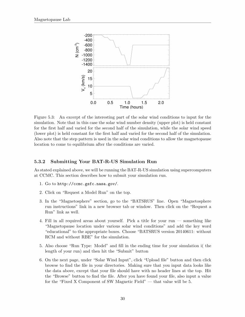
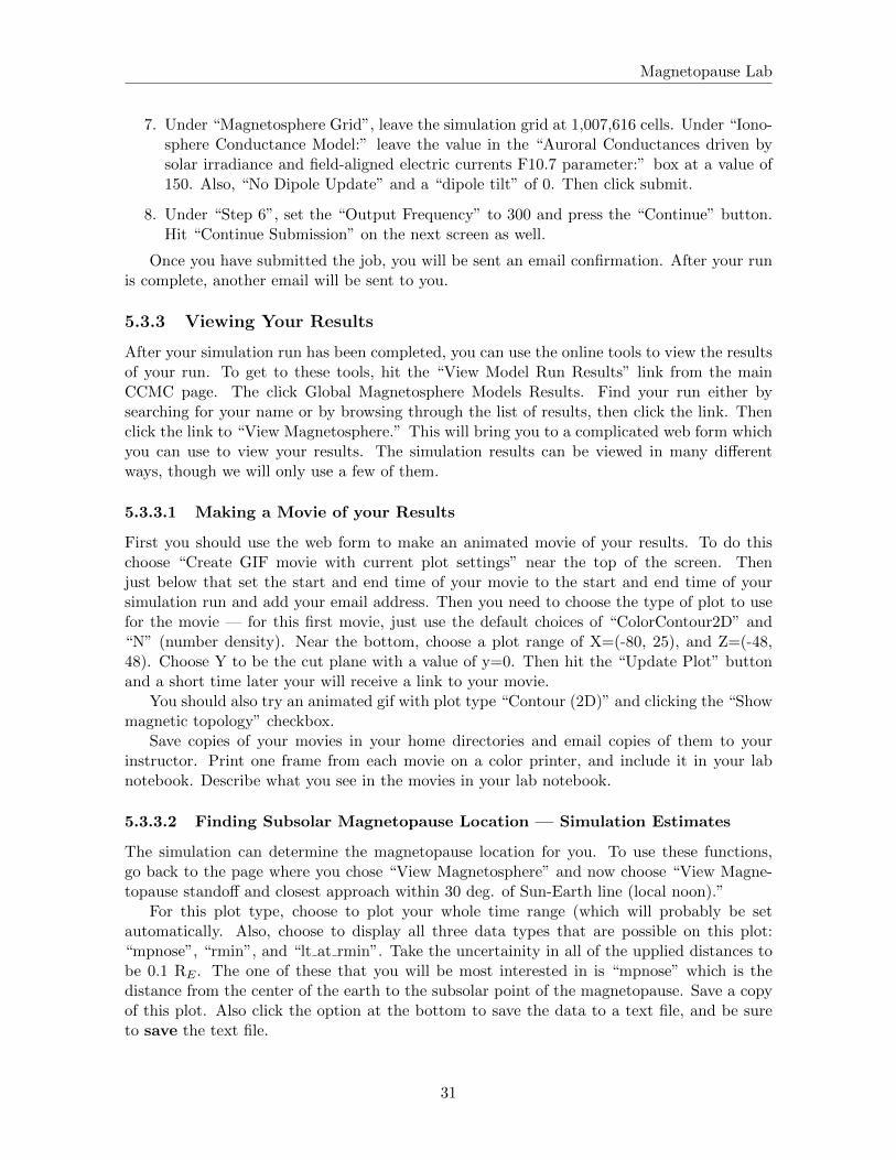
Figure 5.4: Simulation results plot used to find subsolar point of the magnetopause. Thedata are from five minutes into a typical simulation run and they are plotted along the linefrom the Earth to the Sun. The top panel shows the number density, the middle panel showsthe x-component of the plasma flow velocity, and the bottom panel shows z-component of themagnetic field. Geocentric solar magnetospheric (GSM) coordinates are used here.

5.3.3.3 Finding Subsolar Magnetopause Location —Your Interpretations

First you want to choose which time point of your simulation to look at under the “Choosedata time” option. If you used the data input scheme suggested above where the inputparameters are constant for times in a row, then you will want to look at the second time ofeach pair. In order to find the subsolar point of the magnetopause, it easiest to look at a lineplot of various plasma parameters, so choose “Plot Mode” of “Line Plot.” Since the subsolarpoint in on the x-axis, choose “Y1”,“Y2”, “Z1”, “Z2” all equal to 0 under the “Choose PlotArea” section at the bottom of the screen. For the x-limits you will want to start out with arange that is sure to include your magnetopause, and then zoom in once you have found thesubsolar point of the magnetopause. In order to determine your magnetopause, you shouldtake a look at several of the following data quantities: Vx, B, Bx, By, Bz, and n. Figure 5.4is an example of the sort of plot that you will want to make.

The magnetopause boundary should be roughly visible in your plots as the location wherethe plasma parameters are changing rapidly from the solar wind values which you input, tothe magnetosphere values. Recall, though there there are two boundaries near each other inthis region. The bow shock, which separates the solar wind from the magnetosheath and themagnetopause which separates the magnetosheath from the magnetosphere. The key point toremember when searching for the magnetopause location, is that the magnetopause definesthe outer boundary of the region where the earth’s magnetic field dominates.

In Figure 5.4, the magnetopause is located at roughly 11 RE . In the number density plot,the bump in the number density corresponds to the buildup of plasma in the magnetosheath,so the inner boundary of that bump corresponds to the magnetopause. In the plot of the

32

Magnetopause Lab

x-component of the velocity, the magnetopause is seen as the location where the value goesto 0, since the plasma from the solar wind is diverted around the magnetosphere at themagnetopause. Finally, in the plot of the z-component of the magnetic field, there is analmost imperceptible shift at 11 RE . So in this case, counter-intuitively, it is easier to find themagnetopause in the plasma results for the the simulation than in the magnetic field results.

Come up with your own standard to decide where the magnetopause is and make surethat you use more than one parameter in making your decision. Note that the point wheretwo lines representing different quantities cross has no physical significance. Based on yourstandard, you should assign a value for the uncertainty of the location of the subsolar pointbased on how precisely you can determine the locations from your plots. Be sure to save theplots that you use for finding the subsolar point to a file. You should include copies of theseplots in your lab notebook. Note that if you defined your input parameters as suggested, thenyou only need to find the magnetopause location for the last time for each of the sets of inputparameters that have the same parameter values.

5.3.3.4 Fits

The distance from the earth to is magnetopause is given roughly by the equation 5.1. Thisequation makes the assumption that the solar wind for a typical momentum flux of 2.6 nPa(nv2) leads to a magnetopause location at about 10RE [Kivelson et al.,1995, p. 171]. This isonly a general prediction of the location of the magnetopause. Plot your two sets of estimatesof the magnetopause location. From your results find your empirical constant factor (similar107.4) for both of your sets of estimates of the magnetopause location. To do this you willneed to fit your data to equation 5.1. You should come up with four fits to this equation: onefor each section of your input data (constant V and constant n for the solar wind) for eachestimate of the magnetopause location [your estimates (Section 5.3.3.3 and the simulation’sestimates (Section 5.3.3.2)].

5.3.4 Questions

1. Watch the movie that you made of your simulation results again and compare the behav-ior of the magnetopause to your input solar wind conditions. Describe what happensto the magnetosphere as the solar wind conditions vary. Pay particular attention towhat happens when there are large changes in the solar wind conditions. How quicklydo changes in the magnetosphere propagate from one end of the magnetosphere to theother?

2. Compare your two sets of estimates of the magnetopause location. Do they agree withinuncertainties? Are there systematic differences between the two? If so, attempt toexplain why.

3. How do those values compare to each other and to 107.4?

4. What are some possible reasons why in the BATRUS model the value for the magne-topause constant (107.4) changes? What approximations are being made when dealingwith MHD in space?

33

Magnetopause Lab

5.4 Spacecraft Data

For this part of the lab, you will be examining what spacecraft observations of the magneto-sphere tell us about the behavior of the magnetopause under extreme solar wind conditionsand how those results compare to the magnetopause models already mentioned. You will usesolar wind data to predict where the magnetopause is in the vicinity of a number of satellitesand you will check to see if the data from those spacecraft show the spacecraft crossing themagnetopause at the predicted times.

Three specific extreme solar wind events will be examined: October 31 2003, July 15 2000(Bastille Day storm), and May 4, 1998. For each event the solar wind data was collected fromthe Advanced Composition Explorer (ACE) satellite from cdaweb.gsfc.nasa.gov. ACE residesat about 210 RE from the earth on the line between the earth and the sun. On board ACEis an array of instruments to measure the solar wind. Solar wind plasma data (SWEPAM)and magnetic field data (MAG) are the two instruments that we will be using data from. TheSWEPAM instrument takes the solar wind velocity, ion density, and ion temperature, whileMAG takes the magnetic field intensity.

Along with ACE data, we will be using data from several other satellites. These satellitesare of several different classes. The GOES satellites are weather satellites and the data thatthey take that is of interest to us is magnetic field data (MAG) and energetic particle data(EP). The L satellites are run by Los Alamos National lab and contain plasma data, lowand high energy ions as well as electron number densities. All GOES and L satellites arein geosynchronous orbit. We will also be using data from two NASA satellites with moreinteresting orbits — Geotail and Polar. Geotail has ion number density and speed data(CPI), and magnetic field data (MGF) that we will be using. Polar has magnetic field (MFE)data that we will be using. During the events listed above these satellites spend at least sometime inside the magnetosphere. The point of this lab is to check the satellite data for signs ofhaving crossed the magnetopause and compare that to predictions of equation 5.2.

5.4.1 Procedure

For each event the earth’s magnetopause location has already been calculated using equa-tion 5.2 based on ACE data which is also included in the spreadsheet. The position of themagnetopause along with the location of a particular satellite. These results are includedin spreadsheet files which have been stored under the data directory on the course web site.These spreadsheets can be read using the “gnumeric” program. The predicted magnetopauselocation and the satellite’s distance from the earth have also been saved into text files endingwith “.txt”, but are otherwise named the same as the spreadsheets. You will need to use thesetext files to create your own plots of the predicted magnetopause crossings. Along with thespreadsheet files are data files which you will want to compare to the magnetopause locationdata. These files contain either magnetic field data, ion number density data, or particle fluxdata. The data files that you will want to use all end in “ nt.txt”.

1. Magnetic field data contains MAG, MFE, or MFG in the file (G0 K0 MAG 65544.txt)the txt is the actual data and the .gif is a graph of the data.

2. Ion data should be in a MPA (L1 K0 MPA 65778.txt) file from which you want the “lowP DENS” info. Or it will be an EP# (G0 K0 EP8 225752.txt) file where a large fluxusually means a transfer between barriers.

34

Magnetopause Lab

Figure 5.5 shows an example of the type of analysis you will be doing with this data,though you do not have to try to get all of the data on one plot. To make your plots, you canuse the the iplot feature of a program called idl. Directions on how to use this program arein the file iplot tutorial.txt.

Depending on the data that you are using, it may be easiest to have one plot with thespacecraft data open and another plot showing the spacecraft position as well as the predictedposition of the magnetopause. If you have the same time scale on each plot, then you cancompare the features on each plot to determine whether the data supports the idea of havingmagnetopause crossings where they are predicted by the other plot.

The example data in Figure 5.5 shows Geotail data from October 31, 2003. On that daya large CME hit Earth, causing auroras that were visible throughout much of the UnitedStates.

The top panel of Figure 5.5 predicts several magnetopause crossings, but the most notablecrossings are at roughly 5:00, 10:00, and 11:00. From 1:30–5:00 and from roughly 10:00–11:00,Geotail is predicted to be inside the magnetosphere. In other words, at those times Figure 5.5shows the magnetopause further from the Earth than the spacecraft is. For most of the rest ofthat day Geotail was inside the magnetosphere. The data in the middle and bottom panels ofFigure 5.5 shows the crossing from inside to outside the magnetosphere at 11:00 and the dataalso shows other magnetopause crossings, though as described below the crossings seen in thedata differ a bit from the predictions. Note that the prediction of the magnetopause locationis based on solar wind data from outside the magnetosphere. The time its takes the solarwind to get to the spacecraft from the place at which it is measured varies, but it typicallyabout 15 minutes. So we should expect to see magnetopause crossings slightly earlier in thepredictions than in the data.

The middle panel of Figure 5.5, which shows the ion flow velocity measured by Geotailand the x-component of the solar wind speed measured by ACE, has three visible regimes.During this day the x-component of the solar wind velocity slowly changes from −1200 km/sto −800 km/s. From 0:00–5:00 most of the Geotail ion flow velocity data is missing. From5:00–11:00 the three components of the ion flow velocity measured by Geotail oscillate nearvalues of −700 km/s, −400 km/s, and 200 km/s respectively. While from 11:00–24:00 they- and z-components oscillate near 0 km/s, and the x-component is based at roughly −1000km/s, with spikes up to almost 0 km/s. The behavior of the x-component during this last timeperiod can be interpreted as being due to the spacecraft being just outside the magnetopausein the magnetosheath. When the x-component is near −1000 km/s it matches the solar windspeed, suggesting that Geotail is outside the magnetopause at those times. The noisiness ofthese measurements of the ion speed in the magnetosheath is likely due to reflection of thesolar wind ions off the magnetopause and the movement of the magnetopause as the solarwind conditions vary.

The velocity measurements act much differently from 5:00–11:00, suggesting that thespacecraft is inside the magnetosphere during those times. Notice that during this time thereare several short time periods where all components of the data have spike which match theirmagnetosheath values. This suggests that during this time period the spacecraft is near themagnetopause boundary and that fluctuations in the solar wind cause the magnetopause tooscillate back and forth across Geotail’s position.

The third panel, showing Geotail’s magnetic field measurements, has similar regions ofbehavior. From 0:00–11:00 all three components have spiky measurements which trend down-

35

Magnetopause Lab

10

12

14

16

18

20

22D

ista

nce

fro

m E

art

h (

RE)

Magnetopause

Spacecraft

-1200

-1000

-800

-600

-400

-200

0

200

Sp

ee

d (

km

/s)

Solar wind vx

Ion vx

Ion vy

Ion vz

5:00 10:00 15:00 20:00Time of Day (UT) on 31 October 2003

0

50

100

150

Ma

gn

etic f

ield

(n

T)

Bx

By + 100

Bz

Figure 5.5: Plots showing Geotail’s magnetopause crossings on 31 October 2003 (color on-line). The top panel shows the Geotail spacecraft’s distance from Earth and the predictedlocation of the magnetopause along the line from the Earth to Geotail based on the ACEspacecraft measurements of solar wind conditions. The second panel shows Geotail’s mea-surements of the ion flow velocity and the x-component of the solar wind speed measuredby ACE, all in geocentric solar ecliptic (GSE) coordinates. The third panel shows Geotailmeasurements of the three components of the magnetic field in GSE coordinates. The bottomplot shows the ion number density measurement by Geotail.

36

Magnetopause Lab

ward. The downward trend is due to the decreasing magnitude of the Earth’s dipole field asGeotail gets further from Earth, while the spikes are due to disturbances in the plasma inthe magnetosphere during this magnetic storm. From 11:00–24:00, the three components aresteadier and oscillate near 10 nT, 5 nT, and −10 nT, respectively. During this time Geotailis in the magnetosheath where the solar wind magnetic field dominates. Note that duringseveral of the spikes in the magnetic field which occur between 0:00 and 11:00, that the mag-netic field matches the magnetosheath values. This supports the idea that the magnetopauseoscillated back and forth past the spacecraft, as was mentioned with the ion velocity data.

The number density plot shows similar behavior. There is a large spike in the numberdensity just after 5. That peak slowly decays until about 10, after which there are severalsmaller peaks. Once again, this plot shows Geotail inside the magnetopause from roughly5-10, and in the magnetosheath afterwards.

For the cases you will look at, for each satellite there is some sort of data you shouldexamine to try to confirm the location of the magnetopause. In some cases the satellite nevercrosses the theoretical magnetopause, but you need to check that the data shows the samething. When examining the satellite data, pay particular attention to the times at which thetheoretical magnetopause location plot shows the satellite crossing the magnetopause. Noteany signs of a magnetopause crossing. Based on your examination of the data and the theo-retical magnetopause location, determine if you believe the satellite crossed the magnetopauseand if so at what time[s].

***Be sure to analyze potential magnetopause crossings in each set of databefore going on to the questions.*** As part of that analysis, you should describewhether each data plot supports any potential crossings that you see in the spacecraft position/ predicted magnetopause position plot. It is a good practice to write that analysis on thepage you taped made the plot, or on the facing page.

Listed below are the events and the data that we have available for them. Your instructorwill tell you which events you should look at.

Event May 4, 1998 July 15, 2000 October 31, 2003

Satellites GOES 9 GOES 8 GeotailL4 GOES 10 GOES 10L7 L1 GOES 12Polar L4 L0

L9 L1L4L7

5.4.2 Questions

1. For which satellite and event pairs did you find magnetopause crossings? How strongdo you believe the evidence is for a crossing in this case?

2. In any of your events does it appear that the satellite crossed the magnetopause repeat-edly? If so, does it seem as though magnetopause is moving back and forth over thesatellite? What could explain this type of behavior?

3. Which data did you find easier to interpret - ion or magnetic field ? Why?

37

Magnetopause Lab

4. Which spacecraft data did you find easier to interpret? Why? Do you think that thisis a result of the behavior of a specific event? Or of the satellite’s position during thatevent?

5. In any of these cases does the data show the magnetopause crossing geosynchronousorbit?

5.4.3 Conclusion

For this experiment (and the others) you should add a conclusion discussing and critiquingthe lab and your results.

5.5 Acknowledgments

Simulation results have been provided by the Community Coordinated Modeling Center atGoddard Space Flight Center through their public Runs on Request system. The CCMC isa multi-agency partnership between NASA, AFMC, AFOSR, AFRL, AFWA, NOAA, NSFand ONR. The BAT-R-US Model was developed by Tamas Gombosi et al. at the Centerfor Space Environment Modeling at the University of Michigan. Spacecraft key parameterdata provided by CDAWeb. Solar wind data shown here is from ACE SWEPAM providedby D. J. McComas from SWRI and ACE MFI provided by N. Ness from Bartol Re- searchInstitute. Data shown here from Geotail MGF provided by S. Kokubun at STE- LAB, NagoyaUniversity, and Geotail CPI pro- vided by L. Frank at University of Iowa. GOES 8, 9,10, and12 data provided by T. Onsager and H. Singer from NOAA. L1, L4, L7, and L9 data shownhere was provided by provided by E. Dors, M. Thomsen, and D. McComas from LANL. GOES8, 9,10, and 12 data shown here was provided by T. Onsager and H. Singer from NOAA. Polardata shown here was provided by C. Russell (UCLA), D Gurnett (U. Iowa) and W.K. Peterson(LASP/University of Colorado).

5.6 Bibliography

ESA, Coordinate systems and transformations, http://www.spenvis.oma.be/spenvis/

help/background/coortran/coortran.html, 2005.

Hansen, K., G. Toth, A. Ridley, and D. DeZeeuw, BATS-R-US User Manual: Code Version7.5.0, http://csem.engin.umich.edu/docs/HTML/USERMANUAL/USERMANUAL.html, 2002.

Kivelson, A., M. G. Kivelson, and C. T. Russell, Introduction to Space Physics, CambridgeUniversity Press, London, 1995.

NASA, http://ccmc.gsfc.nasa.gov/, 2005.

Shue, J.-H., J. K. Chao, H. C. Fu, C. T. Russell, P. Song, K. K. Khurana, and H. J. Singer,A new functional form to study the solar wind control of the magnetopause size and shape,J. Geophys. Res., 102 (a5), 9497–9512, 1997.

Shue, J.-H., et al., Magnetopause location under extreme solar wind conditions, J. Geophys.Res., 103 (A8), 17,691–17,700, 1998.

38

Speed of Sound Lab

I believe the use of noise to make music will increase until we reach a musicproduced through the aid of electrical instruments which will make available formusical purposes any and all sounds that can be heard.

composer John Cage, 1937

6.1 Introduction

There are many ways to determine the speed of sound. The method we will use in this lab isboth fairly straight forward and the equipment needed is fairly minimal. We will be creatingsounds and recording them with two microphones. We will measure the difference in distancebetween the paths the sounds take from going to the two microphones. We will then study therecorded signals of the sound to see the time difference between how long the sound took toget to each microphone. Our measurement of the speed of sound will be the result of dividingthe difference in distance by the difference in time.

6.1.1 Theory

Sound is a vibrational wave that travels through a medium. The speed of sound in a mediumdepends on how quickly the energy of the vibration can be transferred across the medium.While the details of the equations that are used to find the speed of sound will vary dependingon the state of the medium, the basic equation

∂2u

∂t2= c2∇2u (6.1)

describes the wave where u describes the medium the wave is moving through, and c is thespeed of the wave [Hecht and Zajac, 1987].

In a sound wave, the general method to find the speed is from

vs =

öp

∂ρ(6.2)

where p is the pressure and ρ is the mass density [Landau and Lifshitz , 1993]. In fluids, thespeed can be recast in terms of the bulk modulus, B,

vs =

√B

ρ(6.3)

39

Speed of Sound Lab

which describes the change in volume undergone by a medium when the pressure changes[Halliday et al., 2001]. Similarly, in a solid the sound speed depends on the Young’s modulus,Y ,

vs =

√Y

ρ(6.4)

which describes the stress divided by the strain.

For gases, the bulk modulus is not always easy deal with, since it will in general vary withtemperature, pressure, and density. So the speed of sound equation is often recast using theterms of ideal gases:

vs =

√γkT

m(6.5)

where γ is adiabatic index (which is equivalent to the specific heat at constant pressure dividedby the specific heat at constant volume), k is Boltzmann’s constant, T is the temperature andm is the molecular mass [Landau and Lifshitz , 1993]. For dry air we will take γ = 1.4 andm = 28.9645 u. Unfortunately, air is not a perfectly ideal gas, so to determine the speed ofsound more exactly pressure and humidity must be considered. Consideration of these effectsdoes not lead to simple equations, though, so in practice tables or numerical approximationsare typically used.

6.2 Procedure

6.2.1 The Speed of Sound in Air

In this lab we will be using the program audacity on a Linux computer to record soundsreceived by two microphones. Using the provided adapters you will save one microphonessound as the left track of a stereo recording and one as the right track. For all of themeasurements that you make below, be sure to establish reasonable uncertainties and tomake notes in your lab notebook about why you picked the uncertainties that you used.

Record the air temperature, pressure and humidity for the time of your measurements.Currently we have 1 device that will make all three measurements.

Your first order of business is to figure out how you need to use the provided adapters andcords to hook up the microphones to the computer. Once you believe that you have the cordsset up right, open up audacity and configure that program to receive stereo input. Then testeach microphone separately, to be sure that they are providing signals to the correct channel.Once you are convinced that each microphone is working correctly, try both microphones atthe same time. Play with causing a sound closer to one microphone or the other and see ifyour recorded signals make sense.

Once you are convinced that your setup is correctly recording the signals to both micro-phones, take several sets of data that you can use to find the speed of sound. Remember thatthe distance that will go into your calculations is the difference in the path length traveledby the sound to each microphone.

For the time difference between how long it takes the sounds to get to each microphone,first use audacity directly. Zoom in on your recordings, pick notable locations in the soundwaves, and read off the time difference between when those portions of the wave appear in theleft and the right channels. Be sure to assign an uncertainty to the time difference. Be sure

40

Speed of Sound Lab

to print off at least one set of sample signals from audacity and use the plots when explainingyour method. You may need to create a screenshot in order to extract plots from audacity.

Mathematica can be used to increase the precision of your measurements of the timedelays. A file called sound analysis.nb shows examples using some of the commands below.

You should save your files as .wav files from audacity, using Export.

Then open them in Mathematica using:

sdata= Import["filename", "Data"]

c1 = sdata[[{1}]]

c2= sdata[[[{2}]]

ListPlot[c2, PlotRange -> {{1500, 1550}, {-.1, .2}}]

Repeat this process for at least five different path length differences for the sound’s travelto the two microphones. Be sure to have your path difference use the entire range of possiblevalues allowed by the supplied equipment. Plot your results as path length difference versustime delay and fit the line to find a value for the speed of sound in air.

6.2.2 The Speed of Sound in Some Other Material

In this section of the lab you are in charge. Use the techniques that you learned in theprevious section to find the speed of sound in some material other than air. In your labnotebook describe in detail what you do on this portion. Note that you should be verycareful to consider the fact that the sound may travel both through the material that you areattempting to test and the air.

6.3 Conclusions

1. Find online or in a book a source for the speed of sound in air that considers temperature,humidity, and pressure. This source may have equations, tables, or web forms that givethe speed of sound. Cite your source. Find the speed of sound using equation 6.5 andyour source and compare. Also, try slightly varying the temperature, pressure, andhumidity that you use and see how the results change. Variations in which parametersmake the most difference here? Why? Use these values to come up with a theoreticalvalue of the speed of sound in air with uncertainty for the time of your measurements.Explain how you decided on your value.

2. How do your results for the speed of sound in air compare to the published values? Arethe values consistent to within their uncertainties?

3. What is the published value for the speed of sound in the other material that youtested and what is your source for the speed? (http://www.engineeringtoolbox.com/sound-speed-solids-d_713.html and http://piano-tuners.org/sound.html havesome values.)

How do your results compare to the published values? Are the values consistent towithin their uncertainties?

41

Speed of Sound Lab

4. How could this lab be improved to increase the precision and accuracy of the measure-ments of the speed of sound for air or for other materials?

6.4 Bibliography

Halliday, D., R. Resnick, and J. Walker, Fundamentals of Physics, sixth ed., Wiley, 2001.

Hecht, E., and A. Zajac, Optics, second ed., Addison-Wesley, 1987.

Landau, L. D., and E. M. Lifshitz, Fluid Mechanics, second ed., Pergamon Press, 1993.

42

Torsion Pendulum Lab

Life swings like a pendulum backward and forward between pain and boredom.

Arthur Schopenhauer

7.1 Introduction

Oscillations show up throughout physics. From simple spring systems in mechanics to atomicbonds in quantum physics to bridges blowing the wind, physical systems often act like oscil-lators when they are displaced from stable equilibria.

In this experiment you will observe the behavior of a simple sort of oscillator: the torsionpendulum. In general a torsion pendulum is an object that has oscillations which are dueto rotations about some axis through the object. This apparatus allows for exploring bothdamped oscillations and forced oscillations.

7.2 Theory

Note that angular frequency (ω in rad/s) and frequency (f in Hz.) are not the same. Mostthe equations below concern ω, in many cases it is easier to measure f .

In the damped case, the torque balance for the torsion pendulum yields the differentialequation:

Jd2θ

dt2+ b

dθ

dt+ cθ = 0 (7.1)

where J is the moment of inertia of the pendulum, b is the damping coefficient, c is therestoring torque constant, and θ is the angle of rotation [Leybold Scientific, 2006a]. Thisequation can be rewritten in the standard form [Thornton and Marion, 2004]:

θ + 2βθ + ω20θ = 0, (7.2)

where the damping constant is β = b2J

and the natural frequency is ω0 =√

cJ

. The generalsolution to this differential equations is:

θ(t) = e−βt[A1e√β2−ω2

0t +A2e−√β2−ω2

0t], (7.3)

with three different types of solutions possible depending on the relationships between ω0 andβ.

43

Torsion Pendulum Lab

In the underdamped case (β < ω0):

θ(t) = θ0e−βt cos (ω1t− γ) (7.4)

with the oscillation frequency ω1 =√ω20 − β2, initial amplitude θ0, and phase γ.

In the critically damped case (β = ω0):

θ(t) = (A+Bt)e−βt. (7.5)

In the overdamped case (β > ω0):

θ(t) = e−βt[A1eω2t +A2e

−ω2t], (7.6)

where ω2 =√β2 − ω2

0.

For the forced oscillation case, an external torque is added to Equation 7.1:

Jd2θ

dt2+ b

dθ

dt+ cθ = τ0 sin (wt), (7.7)

where ω is the driving frequency and τ0 is the driving torque [Leybold Scientific, 2006b]. Thegeneral solution to the differential equation is the sum of the homogeneous solutions (whichare the solutions to the damped case above) plus a particular solution. The particular solutionhas the form:

θ(t) = θm(w) sin (wt− φ) (7.8)

with

θm(ω) =τ0

J√

(ω20 − ω2)2 + (bω/J)2

(7.9)

In this case the resonance frequency is ωr =√ω20 + 2β2 and the phase shift between the

pendulum and the external oscillator is:

tanφ =2βω

ω20 − ω2

(7.10)

7.3 Equipment

In this experiment you will use the torsion pendulum, the power supply for the driving motor,a low voltage power supply for the eddy current damper, two digital multimeters, and a stopwatch.

Figure 7.1 shows the torsion pendulum and associated electronics. The motor which isused to force the pendulum (which will only be used in the second half of the experiment) isshown on the left of the diagram. The eddy current damping device is shown on the bottomof the diagram.

7.3.1 Notes on the Torsion Pendulum

• Do not forget to consider uncertainties in your measurements and calculations.

• Do not allow the current through the eddy current damper to exceed 2 A.

44

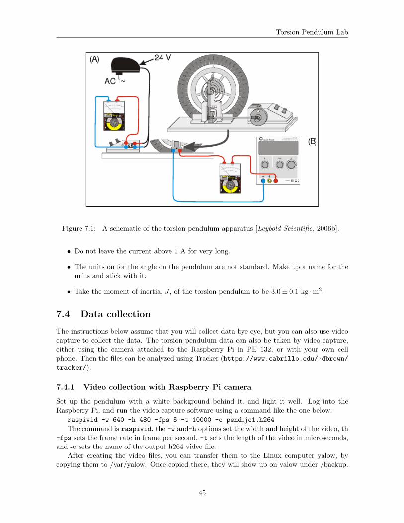
Torsion Pendulum Lab

Figure 7.1: A schematic of the torsion pendulum apparatus [Leybold Scientific, 2006b].

• Do not leave the current above 1 A for very long.

• The units on for the angle on the pendulum are not standard. Make up a name for theunits and stick with it.

• Take the moment of inertia, J , of the torsion pendulum to be 3.0± 0.1 kg ·m2.

7.4 Data collection

The instructions below assume that you will collect data bye eye, but you can also use videocapture to collect the data. The torsion pendulum data can also be taken by video capture,either using the camera attached to the Raspberry Pi in PE 132, or with your own cellphone. Then the files can be analyzed using Tracker (https://www.cabrillo.edu/~dbrown/tracker/).

7.4.1 Video collection with Raspberry Pi camera

Set up the pendulum with a white background behind it, and light it well. Log into theRaspberry Pi, and run the video capture software using a command like the one below:

raspivid -w 640 -h 480 -fps 5 -t 10000 -o pend jc1.h264

The command is raspivid, the -w and-h options set the width and height of the video, th-fps sets the frame rate in frame per second, -t sets the length of the video in microseconds,and -o sets the name of the output h264 video file.

After creating the video files, you can transfer them to the Linux computer yalow, bycopying them to /var/yalow. Once copied there, they will show up on yalow under /backup.

45

Torsion Pendulum Lab

From there, you will need to change the files into mp4 format, so that Tracker can use them:

avconv -i pend jc1.h264 -c copy -r 5 pend jc1.mp4

This command changes the h264 file into an mp4 file, which tracker can deal with. Thecommand avconv can do fancier things like change the frame rate or size of the image as well.(A similar command called ffmpeg is available on the regular Linux computers.)

Tracker

Tracker is currently just installed on yalow. To run it log into yalow from the console, orremotely using ssh:

ssh -Y physics@yalow

Then either find Tracker in the menu, or from a terminal type:

/opt/tracker/tracker.sh

To use Tracker, you can use the fine documentation under Help, particularly GettingStarted. Here’s an even briefer overview:

1. Open your .mp4 video file - other types may work, but not h264.

2. Set the origin. Click on the tool that looks like axes and drag the axes to the center ofthat axis of pendulum.

3. Click Create —Point mass - to pick the tool to follow the pendulum pointer.

4. Shift-click on point on pendulum pointer. Each Shift click advances one frame. Theseclicks digitize the location of the pendulum pointer. The data shows up on the plot.

5. You can display other quantities on your data table by clicking Table and choosing thequantities.

6. You should save your data as a Tracker (.trk) file.

7. Also, save your data as a .txt file for use elsewhere - File—Export—date file .

7.5 Procedure

7.5.1 Damped Oscillations

First, setup the torsion pendulum apparatus, with the forcing motor turned off and play withit to get an idea of how it works [Leybold Scientific, 2006a].

7.5.1.1 Nearly Free Motion

With damping magnet turned off, find the natural frequency by measuring the period ofthe torsion pendulum. You will probably get better results if you use the time it takes thependulum to oscillate 10 or 20 times to find the period. Note that even with the currentoff, friction does cause some damping of the pendulum. So the motion is not quite simpleharmonic motion.

46

Torsion Pendulum Lab

7.5.1.2 Damping Constant

Pick a small value of the damping current (0.1 A < I < 0.3 A) and determine the dampingconstant. To do this first measure the period several times. Then start the pendulum fromits furthest rotation point and measure θmax after each period. If you have difficulty takingthe θmax measurements, you may need to try again. If using video capture, you can just takeone long video at a given damping current, and collect all of the needed information fromthat video.

Plot φmax versus time. Your plot should look like a decreasing exponential. Fit your datato find a value for the damping constant, β.

Repeat this process for a higher value of the damping current (0.3 A < I < 0.6 A).

7.5.1.3 Nearly Critically and Critically Damped

Increase the damping current until the system only completes one oscillation after you let itgo from its furthest rotation point, so the pendulum only crosses 0 once and then approaches 0from the negative side. Find the oscillation time for this case by taking several measurementsand taking the average.

Then increase the current until the pendulum approaches 0 from the positive side, butnever crosses 0. This is the critically damped case. Use several measurements for the time ittakes the pendulum to reach the equilibrium in this case.

Now use the critically damped case to get an estimate of the damping constant, β, in thiscase. Find the damping constant from equation 7.5 by measuring the time that it takes thependulum to reach some fixed θ, say θ0/10, after releasing it from its furthest rotation point.Note that in this case you can assume B = 0 and that A = θ(t = 0) in equation 7.5. Sinceω0 = β in the critically damped case, you can use this β to get estimates of the dampingcoefficient, b, and the restoring torque, c. Recall that J = 3.0± 0.1 kg ·m2.

Now put the current at a higher value (but remember to keep it under 2.0 A). This is anoverdamped case. Find the oscillation time in this case.

7.5.2 Forced Oscillations

First, setup the torsion pendulum apparatus with the forcing motor turned on and play withit to get an idea of how it works [Leybold Scientific, 2006b]. Note that you may have to givethe pendulum an initial displacement to get it moving, but that initial motion will damp out,leaving only the forced oscillations.

7.5.2.1 Resonance Curve

Find the resonance frequency of the torsion pendulum from a amplitude (θmax) versus drivingfrequency plot for the torsion pendulum. In this section, you will need to decide on a procedureyourself, based on what you know about the device and resonance curves. While you are doingtaking data, be sure to note the phase behavior of the driver and the oscillator before, at, andpast resonance. You should find resonance curves and frequencies for three different brake(damping) currents (∼ 0 A, ∼ 0.4 A, and 0.8 A). Also, find the damping constant for thosethree cases.

Note that WAPP has a new option to fit resonance curves. You should attempt to use it,but be skeptical about its results. Your plots must have a fairly well-defined shape near the

47

Torsion Pendulum Lab

peak in order for WAPP to give good results. If WAPP gives suspect results, calculate theresonance frequency by eye from your resonance curve.

7.6 Conclusions

1. Comment on how well the WAPP resonance curve mode works.

2. Are the damping constants in Section 7.5.1.2 consistent with what you would expect?If not, attempt to explain why not.

3. How do the three average oscillation times found in Section 7.5.1.3 compare? Whatdoes this tell you about the critically damped case?

4. In Section 7.5.2.1, how did the phase difference between driver and the oscillator varywith frequency? What was the phase at low frequency? At high frequency? Nearresonance?

5. Considering the damping currents used, are the damping constants found in Sections7.5.1.3, 7.5.1.2 and 7.5.2.1, consistent with each other? If not, attempt to explain whynot.

7.7 Bibliography

Leybold Scientific, Free Rotational Oscillations, Leybold Scientific, http://www.

leybold-didactic.de/literatur/hb/e/p1/p1531_e.pdf, 2006a.

Leybold Scientific, Forced Rotational Oscillations, Leybold Scientific, http://www.

leybold-didactic.de/literatur/hb/e/p1/p1532_e.pdf, 2006b.

Thornton, S. T., and J. B. Marion, Classical Dynamics of Particles and Systems, fifth ed.,Brooks/Cole — Thomson Learning, Belmont, California, 2004.

48