PHYSICAL REVIEW APPLIED 16, 044057 (2021)

Variational Inference with a Quantum Computer

Marcello Benedetti ,1,* Brian Coyle ,1,2 Mattia Fiorentini ,1Michael Lubasch ,1 and Matthias Rosenkranz 1,†

1Cambridge Quantum Computing Limited, London SW1E 6DR, United Kingdom

2School of Informatics, University of Edinburgh, Edinburgh EH8 9AB, United Kingdom

(Received 26 April 2021; revised 17 September 2021; accepted 28 September 2021; published 28 October 2021)

Inference is the task of drawing conclusions about unobserved variables given observations of relatedvariables. Applications range from identifying diseases from symptoms to classifying economic regimesfrom price movements. Unfortunately, performing exact inference is intractable in general. One alter-native is variational inference, where a candidate probability distribution is optimized to approximatethe posterior distribution over unobserved variables. For good approximations, a flexible and highlyexpressive candidate distribution is desirable. In this work, we use quantum Born machines as varia-tional distributions over discrete variables. We apply the framework of operator variational inference toachieve this goal. In particular, we adopt two specific realizations: one with an adversarial objective andone based on the kernelized Stein discrepancy. We demonstrate the approach numerically using exam-ples of Bayesian networks, and implement an experiment on an IBM quantum computer. Our techniquesenable efficient variational inference with distributions beyond those that are efficiently representable ona classical computer.

DOI: 10.1103/PhysRevApplied.16.044057

I. INTRODUCTION

Probabilistic graphical models describe the dependen-cies of random variables in complex systems [1]. Thisframework enables two important tasks: learning andinference. Learning yields a model that approximates theobserved data distribution. Inference uses the model toanswer queries about unobserved variables given obser-vations of other variables. In general, exact inference isintractable and so producing good approximate solutionsbecomes a desirable goal. This article introduces approxi-mate inference solutions using a hybrid quantum-classicalframework.

Prominent examples of probabilistic graphical modelsare Bayesian and Markov networks. Applications acrossmany domains employ inference on those models, includ-ing in health care and medicine [2,3], biology, genetics,and forensics [4,5], finance [6], and fault diagnosis [7].

*marcello.benedetti@cambridgequantum.com†matthias.rosenkranz@cambridgequantum.com

Published by the American Physical Society under the terms ofthe Creative Commons Attribution 4.0 International license. Fur-ther distribution of this work must maintain attribution to theauthor(s) and the published article’s title, journal citation, andDOI.

These are applications where qualifying and quantifyingthe uncertainty of conclusions is crucial. The posterior dis-tribution can be used to quantify this uncertainty. It canalso be used in other downstream tasks such as determin-ing the likeliest configuration of unobserved variables thatbest explains observed data.

Approximate inference methods broadly fall into twocategories: Markov chain Monte Carlo (MCMC) and vari-ational inference (VI). MCMC methods produce samplesfrom the true posterior distribution in an asymptotic limit[8,9]. VI is a machine learning technique that casts infer-ence as an optimization problem over a parameterizedfamily of probability distributions [10]. If quantum com-puters can deliver even a small improvement to thesemethods, the impact across science and engineering couldbe large.

Initial progress in combining MCMC with quantumcomputing was achieved by replacing standard MCMCwith quantum annealing hardware in the training of sometypes of Bayesian and Markov networks [11–17]. Despitepromising empirical results, it proved difficult to show ifand when a quantum advantage could be delivered. Anarguably more promising path towards quantum advantageis through gate-based quantum computers. In this context,there exist algorithms for MCMC with proven asymptoticadvantage [18–21], but they require error correction andother features that go beyond the capability of existingmachines. Researchers have recently shifted their focus to

2331-7019/21/16(4)/044057(18) 044057-1 Published by the American Physical Society

MARCELLO BENEDETTI et al. PHYS. REV. APPLIED 16, 044057 (2021)

near-term machines, proposing new quantum algorithmsfor sampling thermal distributions [22–26].

The advantage of combining quantum computing withVI has not been explored to the same extent as MCMC.Previous work includes classical VI algorithms using ideasfrom quantum annealing [27–29]. In this work, we turnour attention to performing VI on a quantum computer.We adopt a distinct approach that focuses on improvinginference in classical probabilistic models by using quan-tum resources. We use Born machines, which are quantummachine learning models that exhibit high expressivity. Weshow how to employ gradient-based methods and amorti-zation in the training phase. These choices are inspired byrecent advances in classical VI [30].

Finding a quantum advantage in machine learning in anycapacity is an exciting research goal, and promising theo-retical works in this direction have recently been developedacross several prominent subfields. Advantages in super-vised learning have been proposed considering: informa-tion theoretic arguments [31–34], probably approximatelycorrect (PAC) learning [35–38], and the representation ofdata in such models [39–41]. More relevant for our pur-poses are results in unsupervised learning, which haveconsidered complexity and learning theory arguments fordistributions [42–44] and quantum nonlocality and con-textuality [45]. Furthermore, some advantages have beenobserved experimentally [46–49]. For further reading, seeRefs. [50–52] for recent overviews of some advances inquantum machine learning.

In Sec. II we describe VI and its applications. In Sec. IIIwe describe using Born machines to approximate posteriordistributions. In Sec. IV we use the framework of opera-tor VI to derive two suitable objective functions, and weemploy classical techniques to deal with the problematicterms in the objectives. In Sec. V we demonstrate the meth-ods on Bayesian networks. We conclude in Sec. VI with adiscussion of possible generalizations and future work.

II. VARIATIONAL INFERENCE ANDAPPLICATIONS

It is important to clarify what type of inference we arereferring to. Consider a probabilistic model p over someset of random variables, Y . The variables in Y can becontinuous or discrete. Furthermore, assume that we aregiven evidence for some variables in the model. This set ofvariables, denoted X ⊆ Y , is then observed (fixed to thevalues of the evidence) and we use the vector notation x todenote a realization of these observed variables. We nowwant to infer the posterior distribution of the unobservedvariables, those in the set Z := Y\X . Denoting these by avector z, our target is that of computing the posterior distri-bution p(z|x), the conditional probability of z given x. Bydefinition, the conditional can be expressed in terms of thejoint divided by the marginal: p(z|x) = p(x, z)/p(x). Also,

recall that the joint can be written as p(x, z) = p(x|z)p(z).Bayes’ theorem combines the two identities and yieldsp(z|x) = p(x|z)p(z)/p(x).

As described above, the inference problem is rathergeneral. To set the scene, let us discuss some concreteexamples in the context of Bayesian networks. These arecommonly targeted in inference problems, and as suchshall be our test bed for this work. A Bayesian networkdescribes a set of random variables with a clear condi-tional probability structure. This structure is a directedacyclic graph where the conditional probabilities are mod-eled by tables, by explicit distributions, or even by neu-ral networks. Figure 1(a) is the textbook example of aBayesian network for the distribution of binary variables:cloudy (C), sprinkler (S), rain (R), and the grass being wet(W). According to the graph this distribution factorizes asP(C, S, R, W) = P(C)P(S|C)P(R|C)P(W|S, R). A possible

Cloudy

Sprin-kler Rain

Grasswet

(a)

. . .

. . .

(b)

A S Risk factors

T L B DiseasesI

X D Symptoms

(c)

Noisy information bits

Information bits

Codewords

Noisy codewords

(d)

“Sprinkler” network

“Lung cancer” network

Regime switching in time series

Error correction codes

FIG. 1. Some applications of inference on Bayesian networks.Filled (empty) circles indicate observed (unobserved) randomvariables. (a) “Sprinkler” network. (b) Regime switching in timeseries. (c) “Lung cancer” network [53]. (d) Error correctioncodes.

044057-2

VARIATIONAL INFERENCE WITH A QUANTUM COMPUTER PHYS. REV. APPLIED 16, 044057 (2021)

inferential question is: what is the probability distributionof C, S, and R given that W = tr? This can be estimatedby “inverting” the probabilities using Bayes’ theorem:p(C, S, R|W = tr) = p(W = tr|C, S, R)p(C, S, R)/p(W).

Figures 1(b)–1(d) show a few additional applicationsof inference on Bayesian networks. The hidden Markovmodel in Fig. 1(b) describes the joint probability distribu-tion of a time series of asset returns and an unobserved“market regime” (e.g., a booming versus a recessive eco-nomic regime). A typical inference task is to detect regimeswitches by observing asset returns [54]. Figure 1(c) illus-trates a modified version of the “lung cancer” Bayesiannetwork that is an example from medical diagnosis (see,e.g., Ref. [3] and the references therein). This networkencodes expert knowledge about the relationship betweenrisk factors, diseases, and symptoms. In health care, care-ful design of the network and algorithm are critical inorder to reduce biases, e.g., in relation to health care access[55]. Note that inference in medical diagnosis is oftencausal instead of associative [3]. Bayesian networks canbe interpreted causally and help answer causal queriesusing Pearl’s do-calculus [56]. Finally, Fig. 1(d) showsa Bayesian network representation of turbo codes, whichare error correction schemes used in 3G and 4G mobilecommunications. The inference task for the receiver is torecover the original information bits from the informationbits and codewords received over a noisy channel [57].

Inference is a computationally hard task in all butthe simplest probabilistic models. Roth [58] extendedresults of Cooper [59] and showed that exact inferencein Bayesian networks with discrete variables is sharp-P-complete. Dagum and Luby [60] showed that evenapproximate inference is NP-hard. Therefore, unless someparticular constraints are in place, these calculations areintractable. In many cases one is able to perform a “for-ward pass” and obtain unbiased samples from the joint(x, z) ∼ p(x, z) = p(x|z)p(z). However, obtaining unbi-ased samples from the posterior z ∼ p(z|x) = p(x, z)/p(x)is intractable due to the unknown normalization constant.One can perform MCMC sampling by constructing anergodic Markov chain whose stationary distribution is thedesired posterior. MCMC methods have nice theoreticalguarantees, but they may converge slowly in practice [9].In contrast, VI is often faster in high dimensions but doesnot come with guarantees. The idea in VI is to optimizea variational distribution q by minimizing its “distance”from the true posterior p (see Ref. [10] for an introduc-tion to the topic and Ref. [30] for a review of the recentadvances).

VI has experienced a resurgence in recent years dueto substantial developments. First, generic methods havereduced the amount of analytical calculations required andhave made VI much more user friendly (e.g., black-boxVI [61]). Second, machine learning has enabled the useof highly expressive variational distributions implemented

via neural networks [62], probabilistic programs [63],nonparametric models [64], normalizing flows [65], andothers. In contrast, the original VI methods were mostlylimited to analytically tractable distributions such as thosethat could be factorized. Third, amortization methods havereduced the costs by optimizing qθ (z|x) where the vectorof parameters θ is “shared” among all possible observa-tions x instead of optimizing individual parameters foreach observation. This approach can also generalize acrossinferences.

Casting the inference problem as an optimization prob-lem comes itself with challenges, in particular when theunobserved variables are discrete. REINFORCE [66] isa generic method that requires calculation of the score∂θ log qθ (z|x) and may suffer from high variance. Gumbel-softmax reparameterizations [67,68] use a continuousrelaxation that does not follow the exact distribution.

We now show that near-term quantum computers pro-vide an alternative tool for VI. We use the quantum Bornmachine as a candidate for variational distributions. Thesemodels are highly expressive and they naturally representdiscrete distributions as a result of quantum measure-ment. Furthermore, the Born machine can be trained bygradient-based optimization.

III. BORN MACHINES AS IMPLICITVARIATIONAL DISTRIBUTIONS

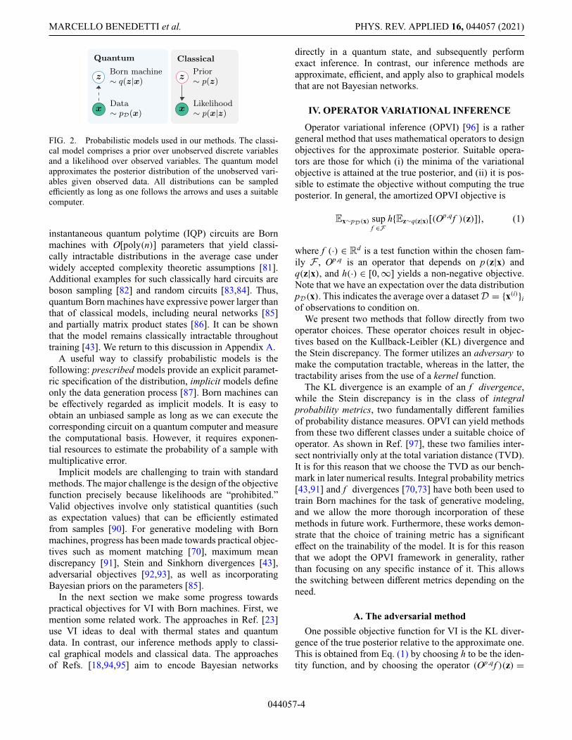
By exploiting the inherent probabilistic nature of quan-tum mechanics, one can model the probability distributionof classical data using a pure quantum state. This modelbased on the Born rule in quantum mechanics is referredto as the Born machine [69]. Let us consider binaryvectors z ∈ {0, 1}n, where n is the number of variables.The Born machine is a normalized quantum state |ψ(θ)〉parameterized by θ that outputs n-bit strings with probabil-ities qθ (z) = |〈z|ψ(θ)〉|2. Here |z〉 are computational basisstates, thus sampling the above probability boils down toa simple measurement. Other forms of discrete variablescan be dealt with by a suitable encoding. When usingamortization, the variational distribution requires condi-tioning on observed variables. To extend the Born machineand include this feature, we let x play the role of addi-tional parameters. This yields a pure state where the outputprobabilities are qθ (z|x) = |〈z|ψ(θ , x)〉|2. Figure 2 showsthe relation between the classical model and the quantummodel for approximate inference.

Born machines have been applied for benchmark-ing hybrid quantum-classical systems [70–73], generativemodeling [74–76], finance [47,48,77], anomaly detection[78], and have been proposed for demonstrating quantumadvantage [43,79]. These models can be realized in a vari-ety of ways, in both classical and quantum computers.When realized via certain classes of quantum circuits, theyare classically intractable to simulate [80]. For example,

044057-3

MARCELLO BENEDETTI et al. PHYS. REV. APPLIED 16, 044057 (2021)

z

x

Born machine∼ q(z|x)

Data∼ pD(x)

Quantum

z

x

Prior∼ p(z)

Likelihood∼ p(x|z)

Classical

FIG. 2. Probabilistic models used in our methods. The classi-cal model comprises a prior over unobserved discrete variablesand a likelihood over observed variables. The quantum modelapproximates the posterior distribution of the unobserved vari-ables given observed data. All distributions can be sampledefficiently as long as one follows the arrows and uses a suitablecomputer.

instantaneous quantum polytime (IQP) circuits are Bornmachines with O[poly(n)] parameters that yield classi-cally intractable distributions in the average case underwidely accepted complexity theoretic assumptions [81].Additional examples for such classically hard circuits areboson sampling [82] and random circuits [83,84]. Thus,quantum Born machines have expressive power larger thanthat of classical models, including neural networks [85]and partially matrix product states [86]. It can be shownthat the model remains classically intractable throughouttraining [43]. We return to this discussion in Appendix A.

A useful way to classify probabilistic models is thefollowing: prescribed models provide an explicit paramet-ric specification of the distribution, implicit models defineonly the data generation process [87]. Born machines canbe effectively regarded as implicit models. It is easy toobtain an unbiased sample as long as we can execute thecorresponding circuit on a quantum computer and measurethe computational basis. However, it requires exponen-tial resources to estimate the probability of a sample withmultiplicative error.

Implicit models are challenging to train with standardmethods. The major challenge is the design of the objectivefunction precisely because likelihoods are “prohibited.”Valid objectives involve only statistical quantities (suchas expectation values) that can be efficiently estimatedfrom samples [90]. For generative modeling with Bornmachines, progress has been made towards practical objec-tives such as moment matching [70], maximum meandiscrepancy [91], Stein and Sinkhorn divergences [43],adversarial objectives [92,93], as well as incorporatingBayesian priors on the parameters [85].

In the next section we make some progress towardspractical objectives for VI with Born machines. First, wemention some related work. The approaches in Ref. [23]use VI ideas to deal with thermal states and quantumdata. In contrast, our inference methods apply to classi-cal graphical models and classical data. The approachesof Refs. [18,94,95] aim to encode Bayesian networks

directly in a quantum state, and subsequently performexact inference. In contrast, our inference methods areapproximate, efficient, and apply also to graphical modelsthat are not Bayesian networks.

IV. OPERATOR VARIATIONAL INFERENCE

Operator variational inference (OPVI) [96] is a rathergeneral method that uses mathematical operators to designobjectives for the approximate posterior. Suitable opera-tors are those for which (i) the minima of the variationalobjective is attained at the true posterior, and (ii) it is pos-sible to estimate the objective without computing the trueposterior. In general, the amortized OPVI objective is

Ex∼pD(x) supf ∈F

h{Ez∼q(z|x)[(Op ,qf )(z)]}, (1)

where f (·) ∈ Rd is a test function within the chosen fam-

ily F , Op ,q is an operator that depends on p(z|x) andq(z|x), and h(·) ∈ [0, ∞] yields a non-negative objective.Note that we have an expectation over the data distributionpD(x). This indicates the average over a dataset D = {x(i)}iof observations to condition on.

We present two methods that follow directly from twooperator choices. These operator choices result in objec-tives based on the Kullback-Leibler (KL) divergence andthe Stein discrepancy. The former utilizes an adversary tomake the computation tractable, whereas in the latter, thetractability arises from the use of a kernel function.

The KL divergence is an example of an f divergence,while the Stein discrepancy is in the class of integralprobability metrics, two fundamentally different familiesof probability distance measures. OPVI can yield methodsfrom these two different classes under a suitable choice ofoperator. As shown in Ref. [97], these two families inter-sect nontrivially only at the total variation distance (TVD).It is for this reason that we choose the TVD as our bench-mark in later numerical results. Integral probability metrics[43,91] and f divergences [70,73] have both been used totrain Born machines for the task of generative modeling,and we allow the more thorough incorporation of thesemethods in future work. Furthermore, these works demon-strate that the choice of training metric has a significanteffect on the trainability of the model. It is for this reasonthat we adopt the OPVI framework in generality, ratherthan focusing on any specific instance of it. This allowsthe switching between different metrics depending on theneed.

A. The adversarial method

One possible objective function for VI is the KL diver-gence of the true posterior relative to the approximate one.This is obtained from Eq. (1) by choosing h to be the iden-tity function, and by choosing the operator (Op ,qf )(z) =

044057-4

VARIATIONAL INFERENCE WITH A QUANTUM COMPUTER PHYS. REV. APPLIED 16, 044057 (2021)

log[q(z|x)/p(z|x)] for all f :

Ex∼pD(x) Ez∼qθ (z|x)

[log

qθ (z|x)p(z|x)

]︸ ︷︷ ︸

Kullback-Leibler divergence

. (2)

Here qθ is the variational distribution parameterized by θ .To avoid singularities we assume that p(z|x) > 0 for all xand all z. The objective’s minimum is zero and is attainedby the true posterior qθ (z|x) = p(z|x) for all x.

There are many ways to rewrite this objective. Herewe focus on the form known as prior contrastive. Substi-tuting Bayes’ formula p(z|x) = p(x|z)p(z)/p(x) into theequation above we obtain

Ex∼pD(x)Ez∼qθ (z|x)

[log

qθ (z|x)p(z)

− log p(x|z)]

+ const.,

(3)

where we ignore the term Ex∼pD(x)[log p(x)] since it isconstant with respect to q. This objective has been usedin many generative models, including the celebrated varia-tional autoencoder (VAE) [62,98]. While the original VAErelies on tractable variational posteriors, one could also usemore powerful, implicit distributions as demonstrated inadversarial variational Bayes [99] and in prior-contrastiveadversarial VI [100].

Let us use a Born machine to model the variationaldistribution qθ (z|x) = |〈z|ψ(θ , x)〉|2. Since this model isimplicit, the ratio qθ (z|x)/p(z) in Eq. (3) cannot be com-puted efficiently. Therefore, we introduce an adversarialmethod for approximately estimating the ratio above. Thekey insight here is that this ratio can be estimated fromthe output of a binary classifier [87]. Suppose that weascribe samples (z, x) ∼ qθ (z|x)pD(x) to the first class,and samples (z, x) ∼ p(z)pD(x) to the second class. Abinary classifier dφ parameterized by φ outputs the prob-ability dφ(z, x) that the pair (z, x) belongs to one of twoclasses. Hence, 1 − dφ(z, x) indicates the probability that(z, x) belongs to the other class. There exist many possiblechoices of objective function for the classifier [87]. In thiswork we consider the cross-entropy

GKL(φ; θ) = Ex∼pD(x)Ez∼qθ (z|x)[log dφ(z, x)]

+ Ex∼pD(x)Ez∼p(z){log[1 − dφ(z, x)]}. (4)

The optimal classifier that maximizes this equation is [99]

d∗(z, x) = qθ (z|x)qθ (z|x)+ p(z)

. (5)

Since the probabilities in Eq. (5) are unknown, the classi-fier must be trained on a dataset of samples. This does notpose a problem because samples from the Born machine

qθ (z|x) and prior p(z) are easy to obtain by assump-tion. Once the classifier is trained, the logit transformationprovides the log odds of a data point coming from theBorn machine joint qθ (z|x)pD(x) versus the prior jointp(z)pD(x). The log odds are an approximation to the logratio of the two distributions, i.e.,

logit[dφ(z, x)] ≡ logdφ(z, x)

1 − dφ(z, x)≈ log

qθ (z|x)p(z)

, (6)

which is exact if dφ is the optimal classifier in Eq. (5). Now,we can avoid the computation of the problematic term inthe KL divergence. Substituting this result into Eq. (3) andignoring the constant term, the final objective for the Bornmachine is

LKL(θ ; φ) = Ex∼pD(x)Ez∼qθ (z|x){logit[dφ(z, x)] − log p(x|z)}. (7)

The optimization can be performed in tandem as

maxφ

GKL(φ; θ),

minθ

LKL(θ ; φ),(8)

using gradient ascent and descent, respectively. It can beshown [99,100] that the gradient of log[qθ (z|x)/p(z)] withrespect to θ vanishes. Thus, under the assumption of anoptimal classifier dφ , the gradient of Eq. (7) is significantlysimplified. This gradient is derived in Appendix B.

A more intuitive interpretation of the procedure justdescribed is as follows. The log likelihood in Eq. (3) canbe expanded as log p(x|z) = log[p(z|x)/p(z)] + log p(x).Then Eq. (3) can be rewritten as Ex∼pD(x)Ez∼qθ (z|x){log[qθ

(z|x)/p(z)] − log[p(z|x)/p(z)]}, revealing the differencebetween two log odds. The first is given by the optimalclassifier in Eq. (6) for the approximate posterior and prior.The second is given by a hypothetical classifier for the trueposterior and prior. The adversarial method is illustrated inFig. 3.

B. The kernelized method

Another possible objective function for VI is the Steindiscrepancy (SD) of the true posterior from the approx-imate one. This is obtained from Eq. (1), assuming thatthe image of f has the same dimension as z, choosing hto be the absolute value, and choosing Op ,q to be a Steinoperator. A Stein operator is independent from q and ischaracterized by having zero expectation under the trueposterior for all functions f in the chosen family F .

044057-5

MARCELLO BENEDETTI et al. PHYS. REV. APPLIED 16, 044057 (2021)

1 Optimize classifierdφ

Vary φ

Prior Born qθ

2 Optimize Born machinePosterior p

Vary θ

Born qθ

Approximation to log odds

Samples from Born machine

FIG. 3. Adversarial variational inference with a Born machine.Step 1 optimizes a classifier dφ to output the probabilities that theobserved samples come from the Born machine rather than fromthe prior. Step 2 optimizes the Born machine qθ to better matchthe true posterior. The updated Born machine is fed back into step1 and the process repeats until convergence of the Born machine.

For binary variables, a possible Stein operator is(Opf )(z) = sp(x, z)Tf (z)− tr[�f (z)], where

[sp(x, z)]i = �zip(x, z)p(x, z)

= 1 − p(x, ¬iz)p(x, z)

(9)

is the difference score function. The partial differenceoperator is defined for any scalar function g on binaryvectors as

�zig(z) = g(z)− g(¬iz), (10)

where ¬iz flips the ith bit in binary vector z. We havealso defined �f (z) as the matrix with entries [�f (z)]ij =�zi fj (z). Under the assumption that p(z|x) > 0 for all xand all z, we show in Appendix C that this is a validStein operator for binary variables. For more general dis-crete variables, we refer the interested reader to Ref. [101].Substituting these definitions into Eq. (1) we obtain [102]:

Ex∼pD(x) supf ∈F

|Ez∼qθ (z|x){sp(x, z)Tf (z)− tr[�f (z)]}|︸ ︷︷ ︸

Stein discrepancy

.

(11)

At this point one can parameterize the test function f andobtain an adversarial objective similar in spirit to that pre-sented in Sec. IV A. Here, however, we take a differentroute. If we take F to be a reproducing kernel Hilbert spaceof vector-valued functions, H, and restricting the Hilbertspace norm of f to be at most one (||f ||H ≤ 1), the supre-mum in Eq. (11) can be calculated in closed form usinga kernel [101]. This is achieved using the “reproducing”properties of kernels, f (z) = 〈k(z, ·), f (·)〉H, substitutinginto Eq. (11) and explicitly solving for the supremum (the

explicit form of this supremal f ∗ is not illuminating for ourdiscussion; see [101] for details). Inserting this f ∗ into theSD results in the kernelized Stein discrepancy (KSD),

Ex∼pD(x)

√Ez,z′∼qθ (z|x)[κp(z, z′|x)]︸ ︷︷ ︸kernelized Stein discrepancy

(12)

where κp is a so-called Stein kernel. For binary variables,this can be written as

κp(z, z′|x) = sp(x, z)Tk(z, z′)sp(x, z′)

− sp(x, z)T�z′k(z, z′)−�zk(z, z′)Tsp(x, z′)

+ tr[�z,z′k(z, z′)]. (13)

Here�zk(z, ·) is the vector of partial differences with com-ponents �zik(z, ·), �z,z′k(z, z′) is the matrix produced byapplying �z to each component of the vector �z′k(·, z′),and tr(·) is the usual trace operation on this matrix. Theexpression κp(z, z′|x) results in a scalar value.

Equation (12) shows that the discrepancy between theapproximate and true posteriors can be calculated fromsamples of the approximate posterior alone. Note thatthe Stein kernel, κp , depends on another kernel k. Forn unobserved Bernoulli variables, one possibility is thegeneric Hamming kernel k(z, z′) = exp[−(1/n)‖z − z′‖1].The KSD is a valid discrepancy measure if this “internal”kernel, k, is positive definite, which is the case for theHamming kernel [101].

1 Compute discrepancy

SD

Ff∗ = sup

f∈F· · ·

Find f∗

F := H

KSD

Hk ⇒ f∗

Explicit f∗

2 Optimize Born machine

Born qθ Posterior p

Vary θ

Discrepancy between Born and posterior

Samples from Born machine, kernel k

FIG. 4. Kernelized Stein variational inference with a Bornmachine. Step 1 computes the Stein discrepancy (SD) betweenthe Born machine and the true posterior using samples from theBorn machine alone. By choosing a reproducing kernel Hilbertspace H with kernel k, the kernelized Stein discrepancy (KSD)can be calculated in closed form. Step 2 optimizes the Bornmachine to reduce the discrepancy. The process repeats untilconvergence.

044057-6

VARIATIONAL INFERENCE WITH A QUANTUM COMPUTER PHYS. REV. APPLIED 16, 044057 (2021)

In summary, constraining ‖f ‖H ≤ 1 in Eq. (11) andsubstituting the KSD we obtain

LKSD(θ) = Ex∼pD(x)

√Ez,z′∼qθ (z|x)[κp(z, z′|x)], (14)

and the problem consists of finding minθ LKSD(θ). Thegradient of Eq. (14) is derived in Appendix D. The ker-nelized method is illustrated in Fig. 4.

The KSD was used in Ref. [43] for generative model-ing with Born machines. In that context the distribution pis unknown; thus, the authors derived methods to approx-imate the score sp from available data. VI is a suitableapplication of the KSD because in this context we do knowthe joint p(z, x). Moreover the score in Eq. (9) can be com-puted efficiently even if we have the joint in unnormalizedform.

V. EXPERIMENTS

To demonstrate our approach, we employ three exper-iments as the subject of the following sections. First,we validate both methods using the canonical “sprin-kler” Bayesian network. Second, we consider continuousobserved variables in a hidden Markov model (HMM), andillustrate how multiple observations can be incorporatedeffectively via amortization. Finally, we consider a largermodel, the “lung cancer” Bayesian network, and demon-strate our methods using an IBM quantum computer.

A. Proof of principle with the “sprinkler” Bayesiannetwork

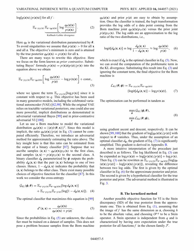
As a first experiment, we classically simulate the meth-ods on the “sprinkler” network in Fig. 1(a), one of thesimplest possible examples. The purpose is to show thatboth methods are expected to work well even when usinglimited resources and without much fine tuning. First, werandomly generate the entries of each probability tablefrom the uniform distribution U([0.01, 0.99]) and pro-duce a total of 30 instances of this network. For eachinstance, we condition on “Grass wet” being true, whichmeans that our data distribution is pD(W) = δ(W = tr). Weinfer the posterior of the remaining three variables usingthe three-qubit version of the hardware-efficient ansatzshown in Fig. 5. We use a layer of Hadamard gates asa state preparation, S(x) = H ⊗ H ⊗ H , and initialize allparameters to approximately 0. Such hardware-efficientansätze, while simple, have been shown to be vulnerableto barren plateaus [103–106], or regions of exponen-tially vanishing gradient magnitudes that make traininguntenable. Alternatively, one could consider ansätze thathave been shown to be somewhat “immune” to this phe-nomenon [107,108], but we leave such investigation tofuture work.

For the KL objective, we utilize a multilayer percep-tron (MLP) classifier made of three input units, six hidden

Repeat for L layers

|0〉

|0〉

|0〉

|0〉

|0〉

S(x)

Rz Rx Rz Rx

Rz Rx Rz Rx

Rz Rx Rz Rx

Rz Rx Rz Rx

Rz Rx Rz Rx

x

∼ pD(x)

z

∼ q(z|x)

FIG. 5. Example of hardware-efficient ansatz for the Bornmachine used in the experiments. All rotations Rx, Rz are param-eterized by individual angles. The layer denoted as S(x) encodesthe values of the observed variables x. The particular choice ofS(x) depends on the application (see the main text). The cor-responding classical random variables are indicated below thecircuit.

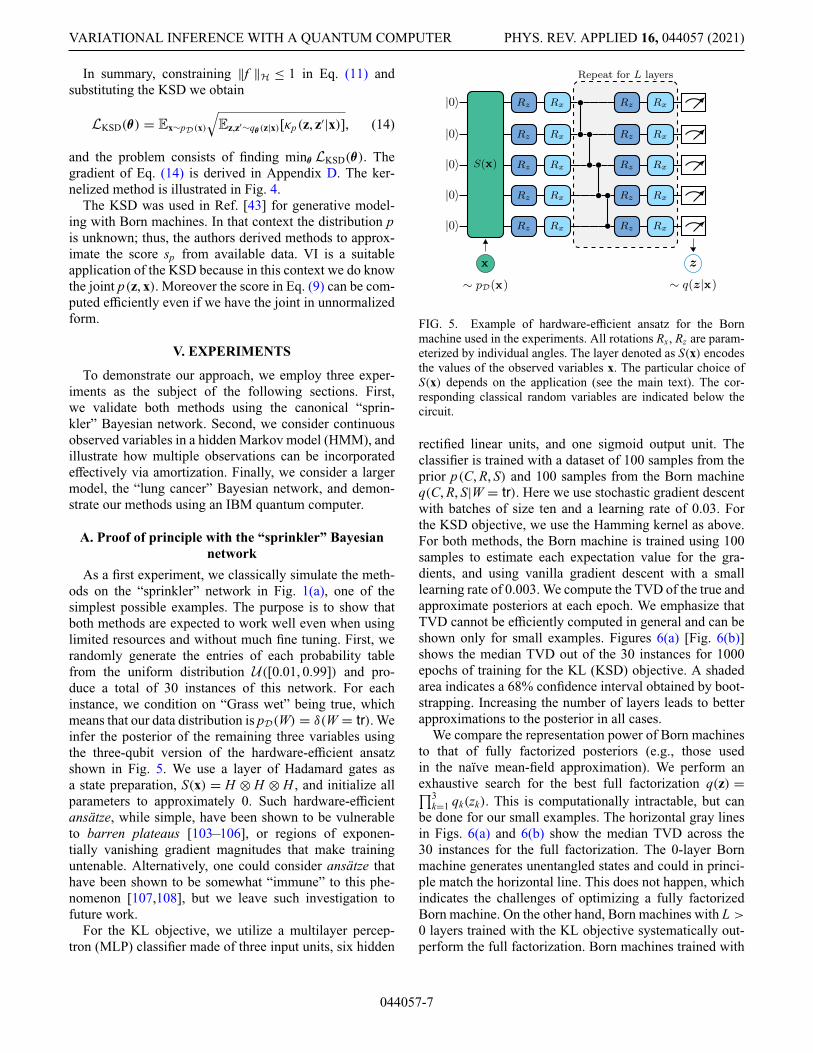
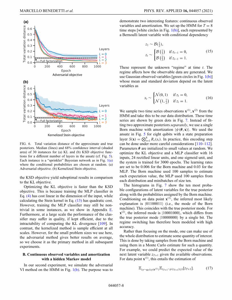
rectified linear units, and one sigmoid output unit. Theclassifier is trained with a dataset of 100 samples from theprior p(C, R, S) and 100 samples from the Born machineq(C, R, S|W = tr). Here we use stochastic gradient descentwith batches of size ten and a learning rate of 0.03. Forthe KSD objective, we use the Hamming kernel as above.For both methods, the Born machine is trained using 100samples to estimate each expectation value for the gra-dients, and using vanilla gradient descent with a smalllearning rate of 0.003. We compute the TVD of the true andapproximate posteriors at each epoch. We emphasize thatTVD cannot be efficiently computed in general and can beshown only for small examples. Figures 6(a) [Fig. 6(b)]shows the median TVD out of the 30 instances for 1000epochs of training for the KL (KSD) objective. A shadedarea indicates a 68% confidence interval obtained by boot-strapping. Increasing the number of layers leads to betterapproximations to the posterior in all cases.

We compare the representation power of Born machinesto that of fully factorized posteriors (e.g., those usedin the naïve mean-field approximation). We perform anexhaustive search for the best full factorization q(z) =∏3

k=1 qk(zk). This is computationally intractable, but canbe done for our small examples. The horizontal gray linesin Figs. 6(a) and 6(b) show the median TVD across the30 instances for the full factorization. The 0-layer Bornmachine generates unentangled states and could in princi-ple match the horizontal line. This does not happen, whichindicates the challenges of optimizing a fully factorizedBorn machine. On the other hand, Born machines with L >0 layers trained with the KL objective systematically out-perform the full factorization. Born machines trained with

044057-7

MARCELLO BENEDETTI et al. PHYS. REV. APPLIED 16, 044057 (2021)

(a)

(b)

Adversarial objective

Kernelized Stein objective

FIG. 6. Total variation distance of the approximate and trueposteriors. Median (lines) and 68% confidence interval (shadedarea) of 30 instances for (a) KL and (b) KSD objective func-tions for a different number of layers in the ansatz (cf. Fig. 5).Each instance is a “sprinkler” Bayesian network as in Fig. 1(a)where the conditional probabilities are chosen at random. (a)Adversarial objective. (b) Kernelized Stein objective.

the KSD objective yield suboptimal results in comparisonto the KL objective.

Optimizing the KL objective is faster than the KSDobjective. This is because training the MLP classifier inEq. (4) has cost linear in the dimension of the input, whilecalculating the Stein kernel in Eq. (13) has quadratic cost.However, training the MLP classifier may still be non-trivial in some instances, as we show in Appendix E.Furthermore, at a large scale the performance of the clas-sifier may suffer in quality, if kept efficient, due to theintractability of computing the KL divergence [109]. Incontrast, the kernelized method is sample efficient at allscales. However, for the small problem sizes we use here,the adversarial method gives better results on average,so we choose it as the primary method in all subsequentexperiments.

B. Continuous observed variables and amortizationwith a hidden Markov model

In our second experiment, we simulate the adversarialVI method on the HMM in Fig. 1(b). The purpose was to

demonstrate two interesting features: continuous observedvariables and amortization. We set up the HMM for T = 8time steps [white circles in Fig. 1(b)], each represented bya Bernoulli latent variable with conditional dependency

z1 ∼ B( 12 ),

zt ∼{B ( 1

3

)if zt−1 = 0,

B ( 23

)if zt−1 = 1.

(15)

These represent the unknown “regime” at time t. Theregime affects how the observable data are generated. Weuse Gaussian observed variables [green circles in Fig. 1(b)]whose mean and standard deviation depend on the latentvariables as

xt ∼{N (0, 1) if zt = 0,

N (1, 1

2

)if zt = 1.

(16)

We sample two time series observations x(1), x(2) from theHMM and take this to be our data distribution. These timeseries are shown by green dots in Fig. 7. Instead of fit-ting two approximate posteriors separately, we use a singleBorn machine with amortization |ψ(θ , x)〉. We used theansatz in Fig. 5 for eight qubits with a state preparationlayer S(x) = ⊗8

t=1 Rx(xt). In practice, this encoding stepcan be done under more careful considerations [110–112].Parameters θ are initialized to small values at random. Weoptimize the KL objective and a MLP classifier with 16inputs, 24 rectified linear units, and one sigmoid unit, andthe system is trained for 3000 epochs. The learning ratesare set to be 0.006 for the Born machine and 0.03 for theMLP. The Born machine used 100 samples to estimateeach expectation value, the MLP used 100 samples fromeach distribution and minibatches of size ten.

The histograms in Fig. 7 show the ten most proba-ble configurations of latent variables for the true posterioralong with the probabilities assigned by the Born machine.Conditioning on data point x(1), the inferred most likelyexplanation is |01100011〉 (i.e., the mode of the Bornmachine). This coincides with the true posterior mode. Forx(2), the inferred mode is |10001000〉, which differs fromthe true posterior mode |10000000〉 by a single bit. Theregime switching has therefore been modeled with highaccuracy.

Rather than focusing on the mode, one can make use ofthe whole distribution to estimate some quantity of interest.This is done by taking samples from the Born machine andusing them in a Monte Carlo estimate for such a quantity.For example, we could predict the expected value of thenext latent variable zT+1 given the available observations.For data point x(1), this entails the estimation of

EzT∼qθ (zT |x(1))EzT+1∼p(zT+1|zT)[zT+1]. (17)

044057-8

VARIATIONAL INFERENCE WITH A QUANTUM COMPUTER PHYS. REV. APPLIED 16, 044057 (2021)

0.00

0.05

0.10

0.15 ��

ModesP

roba

bilit

yTop 10 – True posteriorBorn machine posterior

LatentData

(a)

0.00

0.05

0.10

0.15 ��

Modes

Pro

babi

lity

Top 10 – True posteriorBorn machine posterior

LatentData

(b)

(c) (d)

1 2 3 4 5 6 7 8

−2−1

012

Time step t

Dat

ax(1

)t

Mode of posterior z(1)t

True

Born��

1 2 3 4 5 6 7 8

−2−1

012

Time step tD

ata

x(2)

t

Mode of posterior z(2)t

True

Born��

Posterior histogram given data x(1) Posterior histogram given data x(2)

Time series and posterior modes for x(2)Time series and posterior modes for x(1)

FIG. 7. Truncated, ordered histograms of the posteriors for two observed samples (a) x(1) and (b) x(2) of the hidden Markov model inEqs. (15)–(16). The histograms are sorted by probability of the true posterior. The blue bars are the probabilities of the correspondingapproximate posterior. The x axis shows the latent state for each bar and the observed data point x. The lower panels are the time seriesof the data (c) x(1) and (d) x(2), as well as the corresponding modes of the true posterior and Born machine posterior as indicated withstars in the upper panel. (a) Posterior histogram given data x(1). (b) Posterior histogram given data x(2). (c) Time series and posteriormodes for x(1). (d) Time series and posterior modes for x(2).

To conclude, we mention that inference in this HMM canbe performed exactly and efficiently with classical algo-rithms. The most likely explanation for the observed datacan be found with the Viterbi algorithm in time O(T|S|2),where T is the length of the sequence and |S| is the sizeof the unobserved variables (e.g., |S| = 2 for Bernoullivariables). This is not the case for more general models.For example, a factorial HMM has multiple indepen-dent chains of unobserved variables [113]. Exact inferencecosts O(TM |S|M+1), where M is number of chains, andis typically replaced by approximate inference [113,114].Our VI methods are generic and apply to factorial and otherHMMs without changes.

C. Demonstration on IBMQ with the “lung cancer”Bayesian network

As a final experiment, we test the performance on realquantum hardware using the slightly more complex “lungcancer” network [53], specifically using the five-qubitibmq_rome quantum processor. We access this deviceusing PyQuil [115] and tket [116].

The lung cancer network (also called the “Asia” net-work) is an example of a medical diagnosis Bayesian

network, and is illustrated by Fig. 1(c). This network waschosen since it is small enough to fit without adaptationonto the quantum device, but also comes closer to a “real-world” example. A more complicated version with extravariables can be found in Ref. [117]. We note that the ver-sion we use is slightly modified from that of Ref. [53] fornumerical reasons.

The network has eight variables: two “symptoms” forwhether the patient presented with dyspnoea (D) (shortnessof breath) or had a positive x ray (X ); four possible “dis-eases” causing the symptoms bronchitis (B), tuberculosis(T), lung cancer (L), or an “illness” (I ) (which could beeither tuberculosis or lung cancer or something other thanbronchitis); and two possible “risk factors” for whetherthe patient had traveled to Asia (A) or whether they hada history of smoking (S).

Based on the graph structure in Fig. 1(c), the distri-bution over the variables, p(A, T, S, L, I , X , B, D) can befactorized as

p(A)p(T|A)p(X |I)p(I |T, L)p(D|B, I)p(B|S)p(L|S)p(S).(18)

044057-9

MARCELLO BENEDETTI et al. PHYS. REV. APPLIED 16, 044057 (2021)

0.0

0.1

0.2

Pro

babi

lity

True posteriorBorn machine posterior (simulated)Born machine posterior (hardware)

Config

0 1 2 3 4ibmq rome quantum processor

FIG. 8. Histograms of true versus the learned posteriors with a simulated and hardware trained Born machine for the “lung cancer”network in Fig. 1(c). Here we use the ibmq_rome quantum processor (whose connectivity is shown in the inset). We conditionon X = fa, D = fa, I = tr. The x axis shows the configuration of observed (gray represents X , D, I ) and unobserved variables (bluerepresents A, S, T, L, B) corresponding to each probability (filled circles = tr, empty circles = fa). For hardware results, the histogramis generated using 1024 samples.

In Appendix F we show the explicit probability table weuse (Table I) for completeness. Modifying an illustrativeexample of a potential “real-world” use case in Ref. [53],a patient may present in a clinic with an “illness” (I = tr)but no shortness of breath (D = fa) as a symptom. Fur-thermore, an x ray has revealed a negative result (X = fa).However, we have no patient history and we do not knowwhich underlying disease is actually present. As such, inthe experiment, we condition on having observed the “evi-dence” variables, x: X , D, and I . The remaining five arethe latent variables, z, so we will require five qubits.

In Fig. 8, we show the results when using the five-qubitibmq_rome quantum processor, which has a linear topol-ogy. The topology is convenient since it introduces nomajor overheads when compiling from our ansatz in Fig. 5.We plot the true posterior versus the one learned by theBorn machine both simulated, and on the quantum proces-sor using the best parameters found (after about 400 epochssimulated and about 50 epochs on the processor). To trainin both cases, we use the same classifier as in Sec. V B withfive inputs and ten hidden rectified linear units using theKL objective, which we observed to give the best results.We employ a two-layer ansatz in Fig. 5 (L = 2), and 1024shots are taken from the Born machine in all cases. Weobserve that the simulated Born machine is able to learnthe true posterior very well with these parameters, but theperformance suffers on the hardware. That being said, thetrained hardware model is still able to pick three out of fourhighest probability configurations of the network (shownon the x axis of Fig. 8). The hardware results could likelybe improved with error mitigation techniques.

VI. DISCUSSION

We present two variational inference methods that canexploit highly expressive approximate posteriors given byquantum models. The first method is based on minimizing

the Kullback-Leibler divergence to the true posterior andrelies on a classifier that estimates probability ratios. Theresulting adversarial training may be challenging due to thelarge number of hyperparameters and well-known stabilityissues [118,119]. On the other hand, it only requires theability to (i) sample from the prior p(z), (ii) sample fromthe Born machine qθ (z|x), and (iii) calculate the likelihoodp(x|z). We can apply the method as is when the prior isimplicit. If the likelihood is also implicit, we can refor-mulate Eq. (3) in joint contrastive form [100] and applythe method with minor changes. This opens the possibilityto train a model where both the generative and inferenceprocesses are described by Born machines (i.e., replacingthe classical model in Fig. 2 with a quantum one). Thismodel can be thought of as an alternative way to imple-ment the quantum-assisted Helmholtz machine [15] andthe quantum variational autoencoder [16].

We also present a second VI method based on the ker-nelized Stein discrepancy. A limitation of this approachis that it requires explicit priors and likelihoods. On theother hand, it provides plenty of flexibility in the choiceof kernel. We use a generic Hamming kernel to computesimilarities between bit strings. For VI on graphical mod-els, a graph-based kernel [120] that takes into accountthe structure could yield improved results. Moreover, onecould attempt a demonstration of quantum advantage in VIusing classically intractable kernels arising from quantumcircuits [39–41].

Another interesting extension could be approximatingthe posterior with a Born machine with traced out addi-tional qubits, i.e., locally purified states. This may allowtrading a larger number of qubits for reduced circuit depthat constant expressivity [86].

We present a few examples with direct application tofinancial, medical, and other domains. Another area ofpotential application of our methods is natural languageprocessing. Quantum circuits have been proposed as a

044057-10

VARIATIONAL INFERENCE WITH A QUANTUM COMPUTER PHYS. REV. APPLIED 16, 044057 (2021)

way to encode and compose words to form meanings[121–123]. Question answering with these models couldbe phrased as variational inference on quantum computerswhere our methods fit naturally.

ACKNOWLEDGMENTS

This research was funded by Cambridge Quantum Com-puting. We gratefully acknowledge the cloud comput-ing resources received from the “Microsoft for Startups”program. We acknowledge the use of IBM Quantum Ser-vices for this work. We thank Bert Kappen, Konstanti-nos Meichanetzidis, Robin Lorenz, and David Amaro forhelpful discussions.

APPENDIX A: QUANTUM ADVANTAGE ININFERENCE

The intuitive reason for why approximate inference maybe a suitable candidate for a quantum advantage is simi-lar to that which has already been studied for the relatedproblem of generative modeling using quantum comput-ers [42–45,85]. Here, the primary argument for quantumadvantage reduces to complexity theoretic arguments forthe hardness of sampling from particular probability dis-tributions by any efficient classical means. At one endof the spectrum, the result of Ref. [44] is based on theclassical hardness of the discrete logarithm problem andis not suitable for near-term quantum computers. On theother end, the authors of Refs. [43,85] leveraged argu-ments from “quantum computational supremacy” to showhow Born machines are more expressive than their clas-sical counterparts. Specifically, assuming the noncollapseof the polynomial hierarchy, the Born machine is able torepresent IQP time computations [81].

A similar argument can be made for approximate infer-ence. The key distinction in this case over the previ-ous arguments for generative modeling is that now wemust construct a conditional distribution, the posteriorp(z|x), which at least requires a Born machine to rep-resent it. For an IQP circuit, probability amplitudes aregiven by partition functions of complex Ising models[88,89]. Thus, for a demonstration of quantum advantagein inference, we may seek posterior distributions of theform p(z|x) ∝ |tr(e−iH(z,x))|2. Here the Ising HamiltonianH(z, x) is diagonal and its coefficients depend on both zand x. Alternative “quantum computational supremacy”posteriors could arise from boson sampling [82] and ran-dom circuits [83,84]. In the latter case, experimental val-idations have been performed [124,125], demonstratingthe physical existence of candidate distributions. The for-mer experiment [124] used 53 qubits in the Sycamorequantum chip with 20 “cycles,” where a cycle is a layerof random single-qubit gates interleaved with alternatingtwo-qubit gates. Notably, a cycle is not conceptually verydifferent from a layer in our hardware-efficient ansatz in

Fig. 5 in the main text. The average (isolated) single-(two-)qubit gate error is estimated to be 0.13% (0.36%)in this experiment, which is sufficient to generate a cross-entropy (a measure of distribution “quality,” related to theKL divergence) benchmarking fidelity of 0.1%. The lat-ter [125] repeated this experiment by using 56 qubits fromthe Zuchongzhi processor, again with 20 cycles. In thiscase, the single- (two-)qubit gates carried an average errorof 0.14% (0.59%) to achieve a fidelity of approximately0.07%. Clearly, quantum processors exist that can expressclassically intractable distributions, and so are also likelycapable of representing intractable posterior distributionsfor suitably constructed examples. In all cases, the poste-rior shall be constructed nontrivially from the prior p(z)and likelihood p(x|z) via Bayes’ theorem. We leave thisconstruction for future work. As a final comment, it isalso important to note here that we are discussing onlyrepresentational power and not learnability, which is aseparate issue. It is still unknown whether a distributionfamily (a posterior or otherwise) exists that is learnableby (near-term) quantum means, but not classically. SeeRefs. [43,44] for discussions of this point.

APPENDIX B: GRADIENTS FOR THEADVERSARIAL METHOD

In the adversarial VI method we optimize the objectivefunctions given in Eqs. (4) and (7) via gradient ascent anddescent, respectively. Assuming that the optimal discrim-inator dφ = d∗ has been found, the objective in Eq. (7)becomes

Ex∼pD(x)Ez∼qθ (z|x){logit[d∗(x, z)] − log p(x|z)}. (B1)

While d∗ implicitly depends on θ , the gradient of its expec-tation vanishes. To see this, recall that logit[d∗(z, x)] =log qθ (z|x)− log p(z). Fixing x and taking the partialderivative for the j th parameter,

∂θj

∑z

qθ (z|x) log qθ (z|x) =∑

z

∂θj [qθ (z|x)] log[qθ (z|x)]

+∑

z

qθ (z|x)∂θj [log qθ (z|x)].(B2)

The second term is zero since∑z

qθ (z|x)∂θj [log qθ (z|x)] =∑

z

∂θj qθ (z|x)

= ∂θj

∑z

qθ (z|x)

= ∂θj 1

= 0. (B3)

The approximate posterior in Eq. (B2) is given by theexpectations of observables Oz = |z〉〈z|, i.e., qθ (z|x) =

044057-11

MARCELLO BENEDETTI et al. PHYS. REV. APPLIED 16, 044057 (2021)

〈Oz〉θ ,x. For a circuit parameterized by gates U(θj ) =exp[−i(θj /2)Hj ], where the Hermitian generator Hj haseigenvalues ±1 (e.g., single-qubit rotations), the deriva-tive of the first term in Eq. (B2) can be evaluated with theparameter shift rule [126–128]:

∂θj qθ (z|x) =qθ+

j(z|x)− qθ−

j(z|x)

2(B4)

with θ±j = θ ± (π/2)ej and ej a unit vector in the j th

direction. In summary, the partial derivative of the objec-tive with respect to θj given the optimal discriminator is

12Ex∼pD(x)

(Ez∼q

θ+j(z|x)

{logit[d∗(x, z)] − log p(x|z)}

− Ez∼qθ−

j(z|x){logit[d∗(x, z)] − log p(x|z)}

).

(B5)

APPENDIX C: THE STEIN OPERATOR

Here we prove that (Opf )(z) = sp(x, z)Tf (z)− tr[�f (z)] is a Stein operator for any function f : {0, 1}n →R

n and probability mass function p(z|x) > 0 on {0, 1}n. Todo so, we need to show that its expectation under the trueposterior vanishes. Taking the expectation with respect tothe true posterior we have

Ez∼p(z|x)[(Opf )(z)] =∑

z∈{0,1}n

p(z|x)�p(x, z)T

p(x, z)f (z)

−∑

z∈{0,1}n

p(z|x)tr[�f (z)]. (C1)

The first summation is

∑z∈{0,1}n

1p(x)

�p(x, z)Tf (z)

=∑

z∈{0,1}n

n∑i=1

[p(z|x)− p(¬iz|x)]fi(z), (C2)

while the second summation is∑

z∈{0,1}n

p(z|x)tr[�f (z)]

=∑

z∈{0,1}n

n∑i=1

p(z|x)[fi(z)− fi(¬iz)]. (C3)

Subtracting (C3) from (C2) we have

n∑i=1

[ ∑z∈{0,1}n

p(z|x)fi(z)−∑

z∈{0,1}n

p(¬iz|x)fi(z)

−∑

z∈{0,1}n

p(z|x)fi(z)+∑

z∈{0,1}n

p(z|x)fi(¬iz)]

= 0.

(C4)

The first and third terms cancel. The second and fourthterms are identical and also cancel. This can be seen bysubstituting y i = ¬iz into one of the summations and not-ing that z = ¬iy i. Thus, the operator Op satisfies Stein’sidentity Ez∼p(z|x)[(Opf )(z)] = 0 for any function f asdefined above, and is a valid Stein operator.

APPENDIX D: GRADIENTS FOR THE KERNELIZED METHOD

We wish to optimize the kernelized Stein objective, Eq. (14), via gradient descent. This gradient was derived inRef. [43] and is given by

∂θj LKSD(θ) = ∂θj Ex∼pD(x)

√Ez,z′∼qθ (z|x)[κp(z, z′|x)]

= Ex∼pD(x)∂θj

√Ez,z′∼qθ (z|x)[κp(z, z′|x)]

= 12Ex∼pD(x)

[1√

Ez,z′∼qθ (z|x)[κp(z, z′|x)] {∂θj Ez,z′∼qθ (z|x)[κp(z, z′|x)]}]

= 14Ex∼pD(x)

[1√

Ez,z′∼qθ (z|x)[κp(z, z′|x)]

{E

z∼qθ , z′∼qθ+

j

[κp(z, z′|x)] − Ez∼qθ , z′∼q

θ−j

[κp(z, z′|x)]

+ Ez∼q

θ+j

, z′∼qθ

[κp(z, z′|x)] − Ez∼q

θ−j

, z′∼qθ

[κp(z, z′|x)]}]

. (D1)

044057-12

VARIATIONAL INFERENCE WITH A QUANTUM COMPUTER PHYS. REV. APPLIED 16, 044057 (2021)

The last equality [suppressing the dependence on the vari-ables, z, x: qθ := qθ (z|x)] in Eq. (D1) follows from theparameter shift rule, Eq. (B4), for the gradient of the outputprobabilities of the Born machine circuit, under the sameassumptions as in Appendix B. The relatively simple formof the gradient is due to the fact that the Stein kernel, κp ,does not depend on the variational distribution, qθ (z|x).This gradient can be estimated in a similar way to theKSD itself, by sampling from the original Born machine,qθ (z|x), along with its parameter shifted versions, qθ±

j(z|x)

for each parameter j .

APPENDIX E: LEARNING CURVES FOR THEADVERSARIAL METHOD

In this section we provide examples of successful andunsuccessful VI using the KL objective and adversar-ial methods. We inspect the random instances used inthe “sprinkler” network experiment in Sec. V A. Wecherry-pick two out of the 30 instances where a one-layerBorn machine is employed. Figure 9(a) shows a success-ful experiment. Here the MLP classifier closely tracksthe ideal classifier, providing a good signal for the Bornmachine. The Born machine is able to minimize its loss,which in turn leads to approximately 0 total variationdistance. Figure 9(b) shows an unsuccessful experiment.Here, the MLP tracks the ideal classifier, but the Bornmachine is not able to find a “direction” that minimizesthe loss (see epochs 400 to 1000). We verified that a more

powerful two-layer Born machine performs much betterfor this instance (not shown).

In these figures gray lines correspond to quantities thatcan be estimated from samples, while blue and magentalines represent exact quantities that are not practical tocompute. It is challenging to assess the training looking atthe gray lines. This discussion is to emphasize the need fornew techniques to assess the models. These would providean early stopping criterion for unsuccessful experiments aswell as a validation criterion for successful ones. This is acommon problem among adversarial approaches.

APPENDIX F: PROBABILITY TABLE FOR THE“LUNG CANCER” NETWORK

We derived our VI methods under the assumption ofnonzero posterior probabilities. In tabulated Bayesian net-works, however, zero posterior probabilities may occur.The original “lung cancer” network [53] contains a vari-able “either” (meaning that either lung cancer or tuberculo-sis are present). This variable is a deterministic OR functionof its parent variables and yields zero probabilities in someposterior distributions. In order to avoid numerical issuesarising from zero probabilities, we replace “either” by “ill-ness,” which may be true even if both parent variables“lung cancer” and “tuberculosis” are false. In practice,this is done by adding a small ε > 0 to the entries ofthe “either” table and then renormalizing. This simpletechnique is known as additive smoothing, or Laplace

0 200 400 600 800 10000.0

0.5

1.0

1.5

2.0

2.5

KL loss LKL(θ; φ)

MLP classifier GKL(φ; θ) Ideal classifier

Total variation distance

Epoch

Obje

ctiv

ean

dT

VD

(a)

0 200 400 600 800 10000.0

0.5

1.0

1.5

2.0

2.5

KL loss LKL(θ; φ)

MLP classifier GKL(φ; θ) Ideal classifier

Total variation distance

Epoch

Obje

ctiv

ean

dT

VD

(b)

FIG. 9. Examples of successful (a) and unsuccessful (b) VI on the “sprinkler” Bayesian network in Sec. V A using the KL objectivewith the adversarial method. (a) Successful example. (b) Unsuccessful example.

044057-13

MARCELLO BENEDETTI et al. PHYS. REV. APPLIED 16, 044057 (2021)

TABLE I. Probability table corresponding to the network in Fig. 1(c).

Variable Probabilities Variable Probabilities

Asia (A) p(A = tr) = 0.01 Smoking (S) p(S = tr) = 0.5p(A = fa) = 0.99 p(S = fa) = 0.5

Tuberculosis (T) p(T = tr|A = tr) = 0.05 Illness (I ) p(I = tr|L = tr, T = tr) = 0.95p(T = tr|A = fa) = 0.01 p(I = tr|L = tr, T = fa) = 0.95p(T = fa|A = tr) = 0.95 p(I = tr|L = fa, T = tr) = 0.95p(T = fa|A = fa) = 0.99 p(I = tr|L = fa, T = fa) = 0.05

p(I = fa|L = tr, T = tr) = 0.05Lung cancer (L) p(L = tr|S = tr) = 0.1 p(I = fa|L = tr, T = fa) = 0.05

p(L = tr|S = fa) = 0.01 p(I = fa|L = fa, T = tr) = 0.05p(L = fa|S = tr) = 0.9 p(I = fa|L = fa, T = fa) = 0.95p(L = fa|S = fa) = 0.99

Dyspnoea (D) p(D = tr|B = tr, I = tr) = 0.9Bronchitis (B) p(B = tr|S = tr) = 0.6 p(D = tr|B = tr, I = fa) = 0.8

p(B = tr|S = fa) = 0.3 p(D = tr|B = fa, I = tr) = 0.7p(B = fa|S = tr) = 0.4 p(D = tr|B = fa, I = fa) = 0.1p(B = fa|S = fa) = 0.7 p(D = fa|B = tr, I = tr) = 0.1

p(D = fa|B = tr, I = fa) = 0.2X ray (X ) p(X = tr|I = tr) = 0.98 p(D = fa|B = fa, I = tr) = 0.3

p(X = tr|I = fa) = 0.05 p(D = fa|B = fa, I = fa) = 0.9p(X = fa|I = tr) = 0.02p(X = fa|I = fa) = 0.95

smoothing. Table I shows the modified probability tablefor the network in Fig. 1(c).

An alternative approach to deal with a deterministicvariable that implements the OR function is to marginal-ize its parent variables. It can be verified that the entriesof the resulting probability table are nonzero (unless theparent variables are also deterministic, in which case onemarginalizes these as well). One can perform variationalinference on this modified network with less variables.

[1] D. Koller and N. Friedman, Probabilistic Graphical Mod-els: Principles and Techniques (MIT Press, 2009).

[2] Q. Morris, in Proceedings of the Seventeenth Confer-ence on Uncertainty in Artificial Intelligence (UAI2001),edited by J. Breese and D. Koller (Morgan KaufmannPublishers Inc., Seattle, Washington, USA, 2001), p. 370,ArXiv:1301.2295.

[3] J. G. Richens, C. M. Lee, and S. Johri, Improving the accu-racy of medical diagnosis with causal machine learning,Nat. Commun. 11, 3923 (2020).

[4] M. Maathuis, M. Drton, S. Lauritzen, and M. Wainwright,Handbook of Graphical Models, Chapman & Hall/CRCHandbooks of Modern Statistical Methods (CRC Press,Boca Raton, 2018).

[5] W. Wiegerinck, B. Kappen, and W. Burgers, in InteractiveCollaborative Information Systems, edited by R. Babuškaand F. C. A. Groen (Springer, Berlin, Heidelberg, 2010),p. 547.

[6] A. Denev, Probabilistic Graphical Models: A New Way ofThinking in Financial Modelling (Risk Books, 2015).

[7] B. Cai, L. Huang, and M. Xie, Bayesian networks in faultdiagnosis, IEEE Trans. Ind. Inf. 13, 2227 (2017).

[8] R. M. Neal, Technical Report CRG-TR-93-1, Departmentof Computer Science, University of Toronto, Toronto,1993.

[9] S. Brooks, A. Gelman, G. L. Jones, and X.-L. Meng,eds., Handbook of Markov Chain Monte Carlo Meth-ods (Chapman & Hall/CRC, New York, NY, USA,2011).

[10] D. M. Blei, A. Kucukelbir, and J. D. McAuliffe, Varia-tional inference: A review for statisticians, J. Am. Stat.Assoc. 112, 859 (2017).

[11] S. H. Adachi and M. P. Henderson, Application ofquantum annealing to training of deep neural networks,ArXiv:1510.06356 [quant-ph] (2015).

[12] M. Benedetti, J. Realpe-Gómez, R. Biswas, and A.Perdomo-Ortiz, Estimation of effective temperatures inquantum annealers for sampling applications: A casestudy with possible applications in deep learning,Phys. Rev. A 94, 022308 (2016).

[13] M. Benedetti, J. Realpe-Gómez, R. Biswas, and A.Perdomo-Ortiz, Quantum-Assisted Learning of Hardware-Embedded Probabilistic Graphical Models, Phys. Rev. X7, 041052 (2017).

[14] D. Korenkevych, Y. Xue, Z. Bian, F. Chudak, W. G.Macready, J. Rolfe, and E. Andriyash, Benchmarkingquantum hardware for training of fully visible Boltzmannmachines, ArXiv:1611.04528 [quant-ph] (2016).

[15] M. Benedetti, J. Realpe-Gómez, and A. Perdomo-Ortiz, Quantum-assisted helmholtz machines: A quan-tum–classical deep learning framework for industrialdatasets in near-term devices, Quantum Sci. Technol. 3,034007 (2018).

044057-14

VARIATIONAL INFERENCE WITH A QUANTUM COMPUTER PHYS. REV. APPLIED 16, 044057 (2021)

[16] A. Khoshaman, W. Vinci, B. Denis, E. Andriyash, H.Sadeghi, and M. H. Amin, Quantum variational autoen-coder, Quantum Sci. Technol. 4, 014001 (2018).

[17] M. Wilson, T. Vandal, T. Hogg, and E. G. Rieffel,Quantum-assisted associative adversarial network: Apply-ing quantum annealing in deep learning, Quantum Mach.Intell. 3, 1 (2021).

[18] G. H. Low, T. J. Yoder, and I. L. Chuang, Quantum infer-ence on Bayesian networks, Phys. Rev. A 89, 062315(2014).

[19] A. Montanaro, Quantum speedup of monte carlo methods,Proc. R. Soc. A: Math., Phys. Eng. Sci. 471, 20150301(2015).

[20] A. N. Chowdhury and R. D. Somma, Quantum algorithmsfor gibbs sampling and hitting-time estimation, Quant. Inf.Comp. 17, 0041 (2017). ArXiv:1603.02940 [quant-ph].

[21] P. Wittek and C. Gogolin, Quantum enhanced inference inMarkov logic networks, Sci. Rep. 7 (2017).

[22] J. Wu and T. H. Hsieh, Variational Thermal Quantum Sim-ulation via Thermofield Double States, Phys. Rev. Lett.123, 220502 (2019).

[23] G. Verdon, J. Marks, S. Nanda, S. Leichenauer,and J. Hidary, Quantum Hamiltonian-Based Modelsand the Variational Quantum Thermalizer Algorithm,ArXiv:1910.02071 [quant-ph] (2019).

[24] A. N. Chowdhury, G. H. Low, and N. Wiebe, A Varia-tional Quantum Algorithm for Preparing Quantum GibbsStates, ArXiv:2002.00055 [quant-ph] (2020).

[25] Y. Wang, G. Li, and X. Wang, Variational quantumGibbs state preparation with a truncated Taylor series,ArXiv:2005.08797 [quant-ph] (2020).

[26] Y. Shingu, Y. Seki, S. Watabe, S. Endo, Y. Matsuzaki,S. Kawabata, T. Nikuni, and H. Hakoshima, Boltzmannmachine learning with a variational quantum algorithm,ArXiv:2007.00876 [quant-ph] (2020).

[27] I. Sato, K. Kurihara, S. Tanaka, H. Nakagawa, and S.Miyashita, in Proceedings of the Twenty-Fifth Confer-ence on Uncertainty in Artificial Intelligence UAI’09(AUAI Press, Arlington, Virginia, USA, 2009), p. 479,ArXiv:1408.2037.

[28] B. O’Gorman, R. Babbush, A. Perdomo-Ortiz, A. Aspuru-Guzik, and V. Smelyanskiy, Bayesian network structurelearning using quantum annealing, Eur. Phys. J. Spec. Top.224, 163 (2015).

[29] H. Miyahara and Y. Sughiyama, Quantum extension ofvariational bayes inference, Phys. Rev. A 98, 022330(2018).

[30] C. Zhang, J. Butepage, H. Kjellstrom, and S. Mandt,Advances in variational inference, ArXiv:1711.05597[cs.LG] (2018).

[31] A. Abbas, D. Sutter, C. Zoufal, A. Lucchi, A. Figalli, andS. Woerner, The power of quantum neural networks, Nat.Comput. Sci. 1, 403 (2021).

[32] H.-Y. Huang, R. Kueng, and J. Preskill, Information-Theoretic Bounds on Quantum Advantage in MachineLearning, Phys. Rev. Lett. 126, 190505 (2021).

[33] K. Poland, K. Beer, and T. J. Osborne, No free lunch forquantum machine learning, ArXiv:2003.14103 [quant-ph](2020).

[34] K. Sharma, M. Cerezo, Z. Holmes, L. Cincio, A. Sorn-borger, and P. J. Coles, Reformulation of the no-free-lunch

theorem for entangled data sets, ArXiv:2007.04900[quant-ph] (2020).

[35] R. A. Servedio and S. J. Gortler, Equivalences andseparations between quantum and classical learnability,SIAM J. Comput. 33, 1067 (2004).

[36] S. Arunachalam and R. de Wolf, Guest column: A surveyof quantum learning theory, ACM SIGACT News 48, 41(2017).

[37] S. Arunachalam and R. d. Wolf, Optimal quantum samplecomplexity of learning algorithms, J. Mach. Learn. Res.19, 1 (2018).

[38] Y. Liu, S. Arunachalam, and K. Temme, A rigorous androbust quantum speed-up in supervised machine learning,Nat. Phys. 17, 1013 (2021).

[39] V. Havlícek, A. D. Córcoles, K. Temme, A. W. Harrow,A. Kandala, J. M. Chow, and J. M. Gambetta, Supervisedlearning with quantum-enhanced feature spaces, Nature567, 209 (2019).

[40] M. Schuld and N. Killoran, Quantum Machine Learningin Feature Hilbert Spaces, Phys. Rev. Lett. 122, 040504(2019).

[41] H.-Y. Huang, M. Broughton, M. Mohseni, R. Babbush,S. Boixo, H. Neven, and J. R. McClean, Power of datain quantum machine learning, Nat. Commun. 12, 2631(2021).

[42] X. Gao, Z.-Y. Zhang, and L.-M. Duan, A quantummachine learning algorithm based on generative models,Sci. Adv. 4, eaat9004 (2018).

[43] B. Coyle, D. Mills, V. Danos, and E. Kashefi, The bornsupremacy: Quantum advantage and training of an isingborn machine, npj Quantum Inf. 6 (2020).

[44] R. Sweke, J.-P. Seifert, D. Hangleiter, and J. Eisert, On thequantum versus classical learnability of discrete distribu-tions, Quantum 5, 417 (2021).

[45] X. Gao, E. R. Anschuetz, S.-T. Wang, J. I. Cirac,and M. D. Lukin, Enhancing Generative Models viaQuantum Correlations, ArXiv:2101.08354 [quant-ph](2021).

[46] D. Ristè, M. P. da Silva, C. A. Ryan, A. W. Cross, A. D.Córcoles, J. A. Smolin, J. M. Gambetta, J. M. Chow, andB. R. Johnson, Demonstration of quantum advantage inmachine learning, npj Quantum Inf. 3, 1 (2017).

[47] B. Coyle, M. Henderson, J. C. J. Le, N. Kumar, M.Paini, and E. Kashefi, Quantum versus classical generativemodelling in finance, Quantum Sci. Technol. 6, 024013(2021).

[48] J. Alcazar, V. Leyton-Ortega, and A. Perdomo-Ortiz, Clas-sical versus quantum models in machine learning: Insightsfrom a finance application, Mach. Learning: Sci. Technol.1, 035003 (2020).

[49] S. Johri, S. Debnath, A. Mocherla, A. Singh, A. Prakash,J. Kim, and I. Kerenidis, Nearest centroid classificationon a trapped ion quantum computer, ArXiv:2012.04145[quant-ph] (2020).

[50] C. Ciliberto, M. Herbster, A. D. Ialongo, M. Pontil, A.Rocchetto, S. Severini, and L. Wossnig, Quantum machinelearning: A classical perspective, Proc. R. Soc. A: Math.,Phys. Eng. Sci. 474, 20170551 (2018).

[51] M. Benedetti, E. Lloyd, S. Sack, and M. Fiorentini, Param-eterized quantum circuits as machine learning models,Quantum Sci. Technol. 4, 043001 (2019).

044057-15

MARCELLO BENEDETTI et al. PHYS. REV. APPLIED 16, 044057 (2021)

[52] L. Lamata, Quantum machine learning and quantumbiomimetics: A perspective, Mach. Learning: Sci. Tech-nol. 1, 033002 (2020).

[53] S. L. Lauritzen and D. J. Spiegelhalter, Local computa-tions with probabilities on graphical structures and theirapplication to expert systems, J. R. Stat. Soc. Ser. B(Methodol.) 50, 157 (1988).

[54] M. Kritzman, S. Page, and D. Turkington, Regime shifts:Implications for dynamic strategies (corrected), Financ.Anal. J. 68, 22 (2012).

[55] Z. Obermeyer, B. Powers, C. Vogeli, and S. Mullainathan,Dissecting racial bias in an algorithm used to manage thehealth of populations, Science 366, 447 (2019).

[56] J. Pearl, Causality: Models, Reasoning and Inference(Cambridge University Press, New York, NY, USA,2009), 2nd ed.

[57] R. McEliece, D. MacKay, and Jung-Fu Cheng, Turbodecoding as an instance of pearl’s “belief propaga-tion” algorithm, IEEE J. Sel Areas Commun. 16, 140(1998).

[58] Dan Roth, On the hardness of approximate reasoning,Artif. Intell. 82, 273 (1996).

[59] G. F. Cooper, The computational complexity of proba-bilistic inference using bayesian belief networks, Artif.Intell. 42, 393 (1990).

[60] P. Dagum and M. Luby, Approximating probabilisticinference in Bayesian belief networks is NP-hard, Artif.Intell. 60, 141 (1993).

[61] R. Ranganath, S. Gerrish, and D. M. Blei, Black boxvariational inference, ArXiv:1401.0118 [stat.ML] (2013).

[62] D. P. Kingma and M. Welling, Auto-encoding variationalBayes, ArXiv:1312.6114 [stat.ML] (2014).

[63] D. Wingate and T. Weber, Automated variational infer-ence in probabilistic programming, ArXiv:1301.1299[stat.ML] (2013).

[64] S. Gershman, M. Hoffman, and D. Blei, Nonpara-metric variational inference, ArXiv:1206.4665 [cs.LG](2012).

[65] D. J. Rezende and S. Mohamed, in Proceedings ofthe 32nd International Conference on Machine Learn-ing (PMLR, 2015), Vol. 37, p. 1530, ArXiv:1505.05770[stat.ML].

[66] R. J. Williams, Simple statistical gradient-following algo-rithms for connectionist reinforcement learning, Mach.Learn. 8, 229 (1992).

[67] C. J. Maddison, A. Mnih, and Y. W. Teh, The concretedistribution: A continuous relaxation of discrete randomvariables, ArXiv:1611.00712 [cs.LG] (2017).

[68] E. Jang, S. Gu, and B. Poole, Categorical reparameteriza-tion with gumbel-softmax, ArXiv:1611.01144 [stat.ML](2017).

[69] S. Cheng, J. Chen, and L. Wang, Information perspectiveto probabilistic modeling: Boltzmann machines versusborn machines, Entropy 20, 583 (2018).

[70] M. Benedetti, D. Garcia-Pintos, O. Perdomo, V. Leyton-Ortega, Y. Nam, and A. Perdomo-Ortiz, A generativemodeling approach for benchmarking and training shal-low quantum circuits, npj Quantum Inf. 5 (2019).

[71] K. E. Hamilton, E. F. Dumitrescu, and R. C. Pooser, Gen-erative model benchmarks for superconducting qubits,Phys. Rev. A 99, 062323 (2019).

[72] V. Leyton-Ortega, A. Perdomo-Ortiz, and O. Perdomo,Robust implementation of generative modeling withparametrized quantum circuits, Quantum Mach. Intell. 3,17 (2021).

[73] D. Zhu, N. M. Linke, M. Benedetti, K. A. Landsman,N. H. Nguyen, C. H. Alderete, A. Perdomo-Ortiz, N.Korda, A. Garfoot, C. Brecque, L. Egan, O. Perdomo,and C. Monroe, Training of quantum circuits on a hybridquantum computer, Sci. Adv. 5 (2019).

[74] Z.-Y. Han, J. Wang, H. Fan, L. Wang, and P. Zhang,Unsupervised Generative Modeling Using Matrix ProductStates, Phys. Rev. X 8, 031012 (2018).

[75] M. S. Rudolph, N. B. Toussaint, A. Katabarwa, S. Johri,B. Peropadre, and A. Perdomo-Ortiz, Generation of high-resolution handwritten digits with an ion-trap quantumcomputer, ArXiv:2012.03924 [quant-ph] (2020).

[76] I. Cepaite, B. Coyle, and E. Kashefi, A continuous variableBorn machine, ArXiv:2011.00904 [quant-ph] (2020).

[77] C. Zoufal, A. Lucchi, and S. Woerner, Quantum genera-tive adversarial networks for learning and loading randomdistributions, npj Quantum Inf. 5 (2019).

[78] D. Herr, B. Obert, and M. Rosenkranz, Anomaly detectionwith variational quantum generative adversarial networks,Quantum Sci. Technol. 6, 045004 (2021).

[79] Some literature (e.g., Ref. [77]) refers to Born machines asquantum generative adversarial networks (QGANs) whenusing an adversarial objective function. It is more appro-priate to reserve the term QGAN to adversarial methodsfor quantum data (e.g., Refs. [129–131]).

[80] A quantum computer cannot efficiently implement arbi-trary circuits; thus, some Born machines are intractableeven for a quantum computer.

[81] M. J. Bremner, A. Montanaro, and D. J. Shepherd,Average-Case Complexity versus Approximate Simula-tion of Commuting Quantum Computations, Phys. Rev.Lett. 117, 080501 (2016).

[82] S. Aaronson and A. Arkhipov, in Proceedings of theForty-Third Annual ACM Symposium on Theory of Com-puting, STOC’11 (Association for Computing Machinery,New York, NY, USA, 2011), p. 333.

[83] S. Boixo, S. V. Isakov, V. N. Smelyanskiy, R. Babbush,N. Ding, Z. Jiang, M. J. Bremner, J. M. Martinis, andH. Neven, Characterizing quantum supremacy in near-term devices, Nat. Phys. 14, 595 (2018).

[84] A. Bouland, B. Fefferman, C. Nirkhe, and U. Vazirani, Onthe complexity and verification of quantum random circuitsampling, Nat. Phys. 15, 159 (2019).

[85] Y. Du, M.-H. Hsieh, T. Liu, and D. Tao, Expressivepower of parametrized quantum circuits, Phys. Rev. Res.2 (2020).

[86] I. Glasser, R. Sweke, N. Pancotti, J. Eisert, and I. Cirac,in Advances in Neural Information Processing Systems,edited by H. Wallach, H. Larochelle, A. Beygelzimer, F.d’Alché-Buc, E. Fox, and R. Garnett (Curran Associates,Inc., 2019), Vol. 32, p. 1496, ArXiv:1907.03741 [cs.LG].

[87] S. Mohamed and B. Lakshminarayanan, Learning inimplicit generative models, ArXiv:1610.03483 [stat.ML](2017).

[88] G. D. las Cuevas, W. Dür, M. V. den Nest, and M. A.Martin-Delgado, Quantum algorithms for classical latticemodels, New J. Phys. 13, 093021 (2011).

044057-16

VARIATIONAL INFERENCE WITH A QUANTUM COMPUTER PHYS. REV. APPLIED 16, 044057 (2021)

[89] K. Fujii and T. Morimae, Commuting quantum circuitsand complexity of ising partition functions, New J. Phys.19, 033003 (2017).

[90] Bias and variance of the estimates need to be analyzed andcontrolled, which is a challenge in itself.

[91] J.-G. Liu and L. Wang, Differentiable learning of quantumcircuit born machines, Phys. Rev. A 98, 062324 (2018).

[92] H. Situ, Z. He, Y. Wang, L. Li, and S. Zheng, Quan-tum generative adversarial network for generating discretedistribution, Inf. Sci. (Ny) 538, 193 (2020).

[93] J. Zeng, Y. Wu, J.-G. Liu, L. Wang, and J. Hu, Learningand inference on generative adversarial quantum circuits,Phys. Rev. A 99, 052306 (2019).

[94] S. E. Borujeni, S. Nannapaneni, N. H. Nguyen, E. C.Behrman, and J. E. Steck, Quantum circuit representa-tion of Bayesian networks, ArXiv:2004.14803 [quant-ph](2020).

[95] R. R. Tucci, Quantum Bayesian nets, Int. J. Mod. Phys. B09, 295 (1995).

[96] R. Ranganath, J. Altosaar, D. Tran, and D. M. Blei, Oper-ator variational inference, ArXiv:1610.09033 [stat.ML](2018).

[97] B. K. Sriperumbudur, K. Fukumizu, A. Gretton, B.Schölkopf, and G. R. G. Lanckriet, On integral prob-ability metrics, φ-divergences and binary classification,ArXiv:0901.2698 [cs.IT] (2009).

[98] D. J. Rezende, S. Mohamed, and D. Wierstra, Stochasticbackpropagation and approximate inference in deep gen-erative models, ArXiv:1401.4082 [stat.ML](2014).

[99] L. Mescheder, S. Nowozin, and A. Geiger, Adversar-ial variational Bayes: Unifying variational autoencodersand generative adversarial networks, ArXiv:1701.04722[cs.LG] (2018).

[100] F. Huszár, Variational inference using implicit distribu-tions, ArXiv:1702.08235 [stat.ML] (2017).

[101] J. Yang, Q. Liu, V. Rao, and J. Neville, in Proceedings ofthe 35th International Conference on Machine Learning,Proceedings of Machine Learning Research, edited by J.Dy and A. Krause (PMLR, 2018), Vol. 80, p. 5561.

[102] In contrast to Ref. [101] but in line with earlier worksuch as Ref. [132] we include the absolute value in thedefinition of the Stein discrepancy.

[103] J. R. McClean, S. Boixo, V. N. Smelyanskiy, R. Babbush,and H. Neven, Barren plateaus in quantum neural networktraining landscapes, Nat. Commun. 9, 4812 (2018).

[104] M. Cerezo, A. Sone, T. Volkoff, L. Cincio, and P. J.Coles, Cost function dependent barren plateaus in shal-low parametrized quantum circuits, Nat. Commun. 12(2021).

[105] S. Wang, E. Fontana, M. Cerezo, K. Sharma, A. Sone,L. Cincio, and P. J. Coles, Noise-induced barren plateausin variational quantum algorithms, ArXiv:2007.14384[quant-ph] (2021).

[106] Z. Holmes, K. Sharma, M. Cerezo, and P. J. Coles, Con-necting ansatz expressibility to gradient magnitudes andbarren plateaus, ArXiv:2101.02138 [quant-ph] (2021).

[107] A. Pesah, M. Cerezo, S. Wang, T. Volkoff, A.T. Sornborger, and P. J. Coles, Absence of barrenplateaus in quantum convolutional neural networks,ArXiv:2011.02966 [quant-ph] (2020).

[108] C. Zhao and X.-S. Gao, Analyzing the barren plateau phe-nomenon in training quantum neural network with theZX-calculus, Quantum 5, 466 (2021).

[109] V. Kontonis, S. Liu, and C. Tzamos, Convergence andsample complexity of SGD in GANs, ArXiv:2012.00732[cs.LG] (2020).

[110] R. LaRose and B. Coyle, Robust data encodings forquantum classifiers, Phys. Rev. A 102, 032420 (2020).

[111] M. Schuld, R. Sweke, and J. J. Meyer, Effect of dataencoding on the expressive power of variational quantum-machine-learning models, Phys. Rev. A 103, 032430(2021).

[112] A. Pérez-Salinas, A. Cervera-Lierta, E. Gil-Fuster, andJ. I. Latorre, Data re-uploading for a universal quantumclassifier, Quantum 4, 226 (2020).

[113] Z. Ghahramani and M. I. Jordan, Factorial hidden Markovmodels, Mach. Learn. 29, 245 (1997).

[114] J. Z. Kolter and T. Jaakkola, in Proceedings of theFifteenth International Conference on Artificial Intel-ligence and Statistics, Proceedings of Machine Learn-ing Research, edited by N. D. Lawrence and M. Giro-lami (PMLR, La Palma, Canary Islands, 2012), Vol. 22,p. 1472.

[115] R. S. Smith, M. J. Curtis, and W. J. Zeng, A practicalquantum instruction set architecture, ArXiv:1608.03355[quant-ph] (2016).

[116] S. Sivarajah, S. Dilkes, A. Cowtan, W. Simmons, A.Edgington, and R. Duncan, t|ket〉: A retargetable com-piler for NISQ devices, Quantum Sci. Technol. 6, 014003(2020).

[117] D. Barber, Bayesian Reasoning and Machine Learn-ing (Cambridge University Press, Cambridge, UK,2012).

[118] M. Arjovsky and L. Bottou, Towards principled methodsfor training generative adversarial networks, ArXiv:1701.04862 [stat.ML] (2017).

[119] M. Lucic, K. Kurach, M. Michalski, S. Gelly, andO. Bousquet, in Proceedings of the 32nd Interna-tional Conference on Neural Information ProcessingSystems, NIPS’18 (Curran Associates Inc., 2018), p. 698,ArXiv:1711.10337 [stat.ML].

[120] R. I. Kondor and J. D. Lafferty, in Proceedings of theNineteenth International Conference on Machine Learn-ing, ICML’02 (Morgan Kaufmann Publishers Inc., SanFrancisco, CA, USA, 2002), p. 315.

[121] B. Coecke, G. de Felice, K. Meichanetzidis, and A. Toumi,Foundations for near-term quantum natural language pro-cessing, ArXiv:2012.03755 [quant-ph] (2020).

[122] K. Meichanetzidis, A. Toumi, G. de Felice, and B. Coecke,Grammar-aware question-answering on quantum comput-ers, ArXiv:2012.03756 [quant-ph] (2020).

[123] R. Lorenz, A. Pearson, K. Meichanetzidis, D. Kartsak-lis, and B. Coecke, Qnlp in practice: Running com-positional models of meaning on a quantum computer,ArXiv:2102.12846 [cs.CL] (2021).

[124] F. Arute et al., Quantum supremacy using a pro-grammable superconducting processor, Nature 574, 505(2019).

[125] Y. Wu et al., Strong quantum computational advantageusing a superconducting quantum processor, ArXiv:2106.14734 [quant-ph] (2021).

044057-17

MARCELLO BENEDETTI et al. PHYS. REV. APPLIED 16, 044057 (2021)

[126] K. Mitarai, M. Negoro, M. Kitagawa, and K. Fujii, Quan-tum circuit learning, Phys. Rev. A 98, 032309 (2018).

[127] M. Schuld, V. Bergholm, C. Gogolin, J. Izaac, and N.Killoran, Evaluating analytic gradients on quantum hard-ware, Phys. Rev. A 99, 032331 (2019).

[128] L. Banchi and G. E. Crooks, Measuring analytic gra-dients of general quantum evolution with the stochasticparameter shift rule, Quantum 5, 386 (2021).

[129] P.-L. Dallaire-Demers and N. Killoran, Quantum gen-erative adversarial networks, Phys. Rev. A 98, 012324(2018).

[130] M. Benedetti, E. Grant, L. Wossnig, and S. Severini,Adversarial quantum circuit learning for pure stateapproximation, New J. Phys. 21, 043023 (2019).

[131] S. Chakrabarti, H. Yiming, T. Li, S. Feizi, and X. Wu,in Advances in Neural Information Processing Systems,edited by H. Wallach, H. Larochelle, A. Beygelzimer, F.d’Alché-Buc, E. Fox, and R. Garnett (Curran Associates,Inc., 2019), Vol. 32, p. 6781, ArXiv:1911.00111.

[132] J. Gorham and L. Mackey, Measuring Sample Qualitywith Stein’s Method, ArXiv:1506.03039 [cs, math, stat](2018).

044057-18