PHY 2404S Lecture Notes

Michael Luke

Winter, 2003

These notes are perpetually under construction. Please let me know of anytypos or errors. Once again, large portions of these notes have been plagiarizedfrom Sidney Coleman’s field theory lectures from Harvard, written up by BrianHill.

1

Contents

1 Preliminaries 3

1.1 Counterterms and Divergences: A Simple Example . . . . . . . . 31.2 Counterterms in Scalar Field Theory . . . . . . . . . . . . . . . . 11

2 Reformulating Scattering Theory 18

2.1 Feynman Diagrams with External Lines off the Mass Shell . . . . 182.1.1 Answer One: Part of a Larger Diagram . . . . . . . . . . 192.1.2 Answer Two: The Fourier Transform of a Green Function 202.1.3 Answer Three: The VEV of a String of Heisenberg Fields 22

2.2 Green Functions and Feynman Diagrams . . . . . . . . . . . . . . 232.3 The LSZ Reduction Formula . . . . . . . . . . . . . . . . . . . . 27

2.3.1 Proof of the LSZ Reduction Formula . . . . . . . . . . . . 29

3 Renormalizing Scalar Field Theory 36

3.1 The Two-Point Function: Wavefunction Renormalization . . . . 373.2 The Analytic Structure of G(2), and 1PI Green Functions . . . . 403.3 Calculation of Π(k2) to order g2 . . . . . . . . . . . . . . . . . . 443.4 The definition of g . . . . . . . . . . . . . . . . . . . . . . . . . . 503.5 Unstable Particles and the Optical Theorem . . . . . . . . . . . . 513.6 Renormalizability . . . . . . . . . . . . . . . . . . . . . . . . . . . 57

4 Renormalizability 60

4.1 Degrees of Divergence . . . . . . . . . . . . . . . . . . . . . . . . 604.2 Renormalization of QED . . . . . . . . . . . . . . . . . . . . . . . 65

4.2.1 Troubles with Vector Fields . . . . . . . . . . . . . . . . . 654.2.2 Counterterms . . . . . . . . . . . . . . . . . . . . . . . . . 66

2

1 Preliminaries

1.1 Counterterms and Divergences: A Simple Example

In the last semester we considered a variety of field theories, and learned tocalculate scattering amplitudes at leading order in perturbation theory. Unfor-tunately, although things were fine as far as we went, the whole basis of ourscattering theory had a gaping hole in it. Recall then when we used Wick’stheorem to calculate S matrix elements between some initial state | i〉 and somefinal state | f〉,

Sfi = 〈f |S| i〉 (1.1)

the incoming and outgoing states | i〉 and | f〉 were considered to be eigenstatesof the free Hamiltonian; that is, n particle Fock states. The idea was that far inthe past or future when the colliding particles are widely separated, they don’tfeel the interactions between them. Thus, the incoming and outgoing statesshould be eigenstates of the free theory.

This is clearly nonsense. Even when an electrons is far away from all otherelectrons, it doesn’t look anything like a single particle Fock state. It carrieswith it an electric field made up of photons: even when well-separated fromother electrons, it is always in a complicated superposition of Fock states. Itdoesn’t look anything like a free electron.

Nevertheless, we had a physical argument that suggested we could still cal-culate using free states in the distant past and future. The argument went asfollows: suppose we replaced the interaction term in the Hamiltonian HI by amodified interaction term,

HI → f(t)HI (1.2)

where f(t) (the “turning on and off function”) is some function which is one att = 0 but which vanishes for large |t|. Since the interaction turns off in the farpast and far future, we are justified in using free states in Eq. (1.1).

The question now is, can we do this without changing the physics? Clearly,if at t = −T/2 I suddenly turned the interaction on (that is, if f(t) were a stepfunction) all hell would break loose, and the scattering process would be drasti-cally altered. Since a free electron is in a horribly complicated superposition ofeigenstates of the full Hamiltonian (just as the electron with its electromagneticfield is in a horribly complicated superposition of eigenstates of the free Hamil-tonian), as soon as I turned the interaction on I would be left in a superpositionof states which looked nothing like a real electron. On the other hand, supposeI were to turn the interaction on slowly, very slowly (that is, adiabatically).Then maybe, just maybe, I would be ok, because if I took a very long timeturning the interaction on, I would expect the free state to slowly acquire aphoton field, and to smoothly, with probability 1, turn into an eigenstate of thefull theory. In this case, f(t) would look something like that shown in Fig. 1.1,in the combined limits T → ∞ (so the interaction is on until the particles arearbitrarily far apart, ∆ → ∞ (so the transition is adiabatic), and ∆/T → 0

3

(so the transition time is much less than the time the particle spends with thecorrect Hamiltonian).

f(t)

t

∆

1

T∆

Figure 1.1: Schematic form of the “turning on and off” function f(t), requiredto define scattering theory when the interaction doesn’t vanish in the far pastor future. In the limit T → ∞, ∆ → ∞,∆/T → 0 the results for the originaltheory should be recovered.

In other words, the scattering process goes something like this: a billionyears before the collision, its interaction with the photon field is turned off, andthe electron is a free particle. Then, over a time of a million years, its chargeis slowly turned on, and the electron picks up a photon cloud. Then at t = 0the fully interacting electron collides with a target, and produces a bunch ofparticles. A billion years later, when they are all well separated, these particlesslowly lose their photon clouds, and a million years later we have a bunch of freeparticles again. (An electron with its interactions turned off is usually knownas a “bare” electron; when it comes along with its photon cloud it’s known asa “dressed” electron). Now this approach clearly won’t work for bound states,since no matter how far in the future you go the constituents never get farenough apart not to feel their interactions. But for a low-budget scatteringtheory it should work. Soon we will develop a hi-tech scattering theory withoutthis kluge, but it will suffice for the moment.

To understand the importance of these considerations, it’s instructive to goback to a problem we have looked at before, that of free field theory with asource, and see how the subtleties with the turning on and off function arise.Let us consider a theory with a time-independent source,

LI = −gρ(~x)ϕ(~x, t), ρ(~x) → 0, |~x| → ∞ (1.3)

(where g is a coupling constant). This looks just like a special case of the problemwe considered before, but in fact it is much more subtle. The difference is thatthe source doesn’t vanish in the far future or the far past, which was implicitin the exact solution we obtained for free field theory with a source. So we aregoing to have to implement our turning on and off function to make sense of it.

Let’s see how this problem shows itself in perturbation theory. Recall fromthe perturbative solution to free field theory with a source that the Feynman

4

rule for the source term is that shown in Fig. 1.2, and that, diagrammatically,k i~(k)Figure 1.2: Feynman rule for a source term ρ(x).

the amplitude for the vacuum to be unchanged in the far future has the pertur-bative expansion shown in Fig. 1.3. Defining α to be the subdiagram with ah0jS 1j0i = + + : : :+ +

Figure 1.3: Perturbative expansion for 〈0 |S − 1| 0〉 in a theory with source.

two sources connected by a meson propagator (not including the factor of 1/2!coming from Wick’s theorem),

α = −ig2

∫

d4k

(2π)4ρ(k)ρ(−k)k2 − µ2 + iǫ

(1.4)

and taking into account the combinatorics of connecting n points, it is simpleto sum the series,

〈0 |S| 0〉 = 1 +1

2!α+

3 × 1

4!α2 +

5 × 3 × 1

6!α3 + . . .

= 1 +(α

2

)

+1

2!

(α

2

)2

+1

3!

(α

2

)3

+ . . .

= eα2 . (1.5)

Now, what do we expect the result to be? Since this is just a theory of astatic arrangement of charges, the system should just sit there. The source istime-independent, so it can’t impart any energy to the system. Thus, it can’tcreate mesons, so the vacuum state can’t change, and we should find

〈0 |S| 0〉 = 1 (1.6)

or α = 0. But this isn’t what we get. Instead, from the expression above, andusing the Fourier transform of a time-independent source (forgetting, for themoment, about f(t))

ρ(k) =

∫

d3k

(2π)3ρ(~x)

∫

dk0

2πeik0t−i

~k·~x

= δ(k0)ρ(~k) (1.7)

5

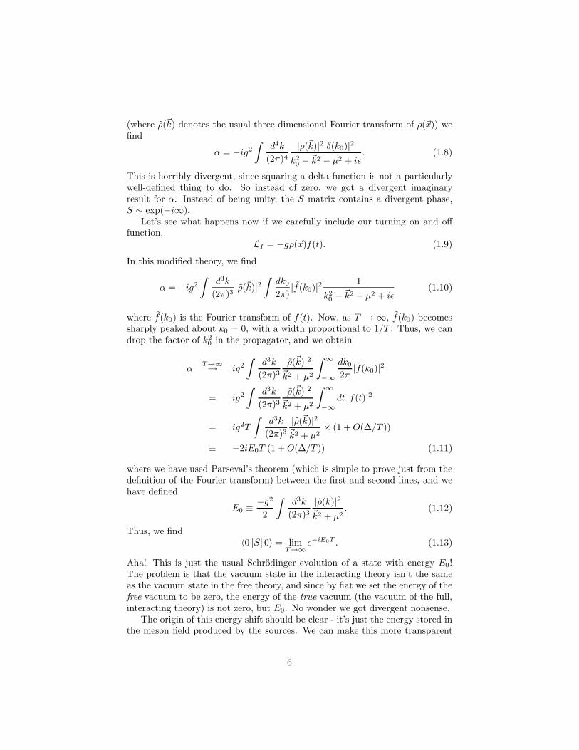
(where ρ(~k) denotes the usual three dimensional Fourier transform of ρ(~x)) wefind

α = −ig2

∫

d4k

(2π)4|ρ(~k)|2|δ(k0)|2

k20 − ~k2 − µ2 + iǫ

. (1.8)

This is horribly divergent, since squaring a delta function is not a particularlywell-defined thing to do. So instead of zero, we got a divergent imaginaryresult for α. Instead of being unity, the S matrix contains a divergent phase,S ∼ exp(−i∞).

Let’s see what happens now if we carefully include our turning on and offfunction,

LI = −gρ(~x)f(t). (1.9)

In this modified theory, we find

α = −ig2

∫

d3k

(2π)3|ρ(~k)|2

∫

dk0

2π)|f(k0)|2

1

k20 − ~k2 − µ2 + iǫ

(1.10)

where f(k0) is the Fourier transform of f(t). Now, as T → ∞, f(k0) becomessharply peaked about k0 = 0, with a width proportional to 1/T . Thus, we candrop the factor of k2

0 in the propagator, and we obtain

αT→∞→ ig2

∫

d3k

(2π)3|ρ(~k)|2~k2 + µ2

∫ ∞

−∞

dk0

2π|f(k0)|2

= ig2

∫

d3k

(2π)3|ρ(~k)|2~k2 + µ2

∫ ∞

−∞

dt |f(t)|2

= ig2T

∫

d3k

(2π)3|ρ(~k)|2~k2 + µ2

× (1 +O(∆/T ))

≡ −2iE0T (1 +O(∆/T )) (1.11)

where we have used Parseval’s theorem (which is simple to prove just from thedefinition of the Fourier transform) between the first and second lines, and wehave defined

E0 ≡ −g2

2

∫

d3k

(2π)3|ρ(~k)|2~k2 + µ2

. (1.12)

Thus, we find〈0 |S| 0〉 = lim

T→∞e−iE0T . (1.13)

Aha! This is just the usual Schrodinger evolution of a state with energy E0!The problem is that the vacuum state in the interacting theory isn’t the sameas the vacuum state in the free theory, and since by fiat we set the energy of thefree vacuum to be zero, the energy of the true vacuum (the vacuum of the full,interacting theory) is not zero, but E0. No wonder we got divergent nonsense.

The origin of this energy shift should be clear - it’s just the energy stored inthe meson field produced by the sources. We can make this more transparent

6

by expressing the potential in position, rather than momentum, space. We canwrite

V (~x) = −g2

∫

d3x

(2π)3ei~k·x

~k2 + µ2

= − g2

4π|~x|e−µ|~x| (1.14)

in terms of which we have

E0 =1

2

∫

d3xd3y ρ(~x)ρ(~y)V (~x− ~y). (1.15)

In analogy with electrostatics, this is just the potential energy of a charge dis-tribution ρ(~x), where the potential between two unit point charges a distancer apart is V (r) (the factor of 1/2 is there because by integrating over ~x and ~yyou double count each pair of point charges). This is the Yukawa potential wediscussed in the context of scattering, and provides another way of seeing theexchange of a scalar boson of mass µ produces an attractive Yukawa potential.In particular, if we consider the source to consist of two almost-point chargesat points ~y1 and ~y2,

ρ(~x) = ∆(~x − ~y1) + ∆(~x − ~y2) (1.16)

where ∆(~x) approaches a δ function, we get

E0 = (something independent of ~y1, ~y2) + V (~y1 − ~y2) (1.17)

The term independent of ~y1 and ~y2 is just the interaction of each “point” chargewith itself, and diverges as ∆(~x) → δ(3)(~x). This is the same problem as thedivergent energy stored in the field of a single point charge in classical electro-dynamics. But since it’s a constant, we don’t care about it: the internucleonpotential V (r), which is the only measurable quantity, is perfectly well-defined.

So now that we understand the origin of the divergent phase, it’s easy to seehow to fix it. We should just define our zero of energy to be the energy of thetrue vacuum, not the free vacuum. Thus, we just add a constant term to theinteraction Hamiltonian,

HI → HI − E0 (1.18)

or, equivalently,LI → LI + E0 (1.19)

or in terms of the Lagrange density,

LI → LI + a (1.20)

where

a ≡ 1

2

∫

d3yρ(~x)ρ(~y)V (~x− ~y) (1.21)

is called a counterterm. This is a term added to the Lagrangian which fixesup the fact that some property of the free theory (such as the vacuum energy)

7

is not the same in the interacting theory, and this must be corrected for. Wewill encounter more of these later on when we start looking at theories withdynamical sources. But for now, using the corrected Lagrangian, we have thenew (rather trivial) interaction shown in Fig. 1.4, which once again exponenti-iaFigure 1.4: Feynman rule corresponding to the vacuum energy counterterm.

ates, precisely cancelling each term of the previous series. Thus, in the modifiedtheory, we find

〈0 |S| 0〉 = 1 (1.22)

as required.A couple of comments:

1. In the case of a point source, ∆(~x) → δ(3)(~x), the counterterm a diverges.Nevertheless, the S matrix element is perfectly finite. The divergent coun-terterm is required to cancel the divergent energy of the field of a pointsource. While this infinity may be scary, it is not harmful. Since terms inthe Lagrangian are not observable, they need not be finite.

2. There is a simpler way to deal with the vacuum energy shift than worryingabout counterterms. Since the disconnected diagrams exponentiate, andevery S-matrix element contains the same set of disconnected diagrams,they contribute a common phase to every S-matrix element. Thus, we canwrite any S-matrix element as

〈k′1, . . . , k′n |S| k1, . . . , km〉 = (sum of connected diagrams)× 〈0 |S| 0〉(1.23)

where, when the counterterm is not included,

〈0 |S| 0〉 = exp (sum of disconnected diagrams) = exp(−iE0T ). (1.24)

Thus, if we adopt the rule of thumb that we only calculate connected di-agrams, we can completely neglect the vacuum energy counterterm. For-mally, this just means that we divide all amplitudes by 〈0 |S| 0〉:

〈k′1, . . . k′n |S| k1, . . . , km〉R =〈k′1, . . . k′n |S| k1, . . . , km〉

〈0 |S| 0〉 . (1.25)

where the subscript R indicates that the vacuum energy has been renor-malized to 0. This will be the approach we take.

Let’s push this model a bit harder. Having found the energy of the true vacuum,let’s find the particle content of the ground state in terms of eigenstates of the

8

free theory. We can find it by using the results for the case of a time-dependentsource, by considering the following form for the source:

ρ(x) = ρ(~x)eǫt, t < 0

ρ(x) = 0, t > 0 (1.26)

and then taking the limit ǫ→ 0+. Physically, what we are doing is turning theinteraction on very slowly, so that the free vacuum smoothly transforms intothe true vacuum of the static theory. Then we turn the interaction abruptlyoff, so that in the interaction picture the state doesn’t evolve at all after t = 0.This is not the same as the theory of a static source, since the interaction isnot adiabatically turned off far in the future. Instead of evolving smoothly backinto the free vacuum, when the source is suddenly turned off the system is leftin the physical vacuum.

Let us denote the vacuum of the static theory by |Ω〉, and the free vacuumas usual by | 0〉. Then the statement that the free vacuum at t = −∞ smoothlytransforms into the physical vacuum at t = 0 may be written as

|Ω〉 = UI(0,−∞)| 0〉 (1.27)

where UI(t1, t2) = T exp(

∫ t2t1dtHI(t)

)

is the usual time-evolution operator.

Furthermore, since the system does not evolve past t = 0, we have UI(t, 0) = 0for any positive time t. The 0 to n meson S-matrix elements may then bewritten

〈~k1, . . . , ~kn |S| 0〉 = 〈~k1, . . . , ~kn |UI(∞,−∞)| 0〉= 〈~k1, . . . , ~kn |UI(0,−∞)| 0〉= 〈~k1, . . . , ~kn|Ω〉 (1.28)

which is exactly what we are looking for: the overlap of the true vacuum withthe n-meson eigenstates of the free theory. Then, using the results for the theorywith a time-dependent source, we recall that the resulting state |Ω〉 is a coherentstate of mesons, and that the probability for the state to contain n mesons is

P (n) =1

n!αn exp(−α) (1.29)

where

α = g2

∫

d3k

(2π)31

2ωk|ρ(k)|2 . (1.30)

From the form of ρ(x), we then find

ρ(k) =

∫

d4xeik·xρ(x)

=

∫

d3xe−i~k·~xρ(~x)

∫ 0

−∞

dt eik0teǫt

9

= ρ(~k)1

ik0 + ǫ

ǫ→0= − i

k0ρ(~k) (1.31)

and therefore

α = g2

∫

d3k

(2π)3|ρ(~k)|22ω3

k

. (1.32)

Now, consider the simple case of a point charge at the origin, ρ(~x) → δ(3)(~x).

In this case, ρ(~k) → 1 for all ~k, and we find, for large |~k|,

α ∼∫

d3k

ω3k

∼∫ ∞ dk

k(1.33)

which is logarithmically divergent: if we only integrate up to |~k| = Λ, the upperlimit of integration will contribute a piece proportional to ln Λ. This is known asan ultraviolet divergence, and looks like bad news. Since the expectation valueof the number of mesons in the ground state 〈Ω |N |Ω〉 = α (from our previousresults), we see that not only the energy of field becomes infinite in the limit ofa point nucleon, but the ground state flees Fock Space. The problem is that apoint source can excite mesons of arbitrarily short wavelength, and arbitrarilyhigh energy. On the other hand, as we have already shown, physically observablequantities do not depend on this unpleasant fact. However, it does mean thatthe vacuum energy counterterm is formally divergent, and that we will have tobe careful to make sure that the theory remains well-defined.

Even if we don’t take the limit of a point source (so that our theory remainsfinite in the ultraviolet) we will also run into difficulties if we take the massless

limit, µ→ 0. In this case, we get, this time for small |~k|,

〈Ω |N |Ω〉 ∼∫

0

d3k

k3∼∫

0

dk

k(1.34)

which is also logarithmically divergent, this time at the lower limit of integration.This is known as an infrared divergence, and corresponds to an infinite numberof mesons with very large wavelengths, and correspondingly very low energies.

While having an infinite number of arbitrarily low-energy particles soundslike trouble, it turns out that this divergence is also unmeasurable. The numberof mesons with arbitrarily small energies is not observable. Any experimenthas only some finite lower limit of energy which it can resolve. Even if thereare 1020 photons with wavelengths between one light year and two light yearshitting your detector, you’ll never see them. It might be a problem if there werean infinite amount of energy stored by these photons, but there isn’t:

〈Ω |H |Ω〉 ∼∫

d3kωkω3k

∼∫

0

dk (1.35)

10

which is finite in the infrared. So, interestingly enough, the number of softmassless mesons (or photons, in QED) is not a physical observable. In gen-eral, infrared divergences signal that you have attempted to calculate somethingwhich is not observable.

To conclude, let me just restate the lessons we have learned from this section.While we have demonstrated them in a simple model, it shouldn’t be hard toconvince yourself that these issues will arise in any interacting field theory.

1. Properties of states of the free theory, such as the vacuum energy, may bedramatically modified by the interaction, and it in general it is necessaryto introduce counterterms into the interaction Lagrangian to correct forthis. This procedure is known as renormalization, and aspects of it willoccupy us for much of this course.

2. When pointlike interacting particles are present, the energy and number ofquanta of the states of the theory both suffer from ultraviolet divergences.Physical quantities are still finite, but this requires the introduction offormally divergent counterterms into the Lagrangian. The procedure ofintroducing an artificial prescription to make such terms finite (for exam-ple, by including a upper cutoff in momentum integrals and at the endtaking the cutoff to infinity) is known as regularization.

3. When massless particles are present, the theory will have infrared diver-

gences, resulting from the fact that there may be an arbitrarily large num-ber of unobservably low-energy quanta in a state. Infrared divergences ina calculation indicate that an observable quantity (such as the number ofsoft photons in a state) is being calculated. Physical quantities (such asthe energy difference between two states) are well-defined.

1.2 Counterterms in Scalar Field Theory

We now consider a more interesting theory with dynamics, and see how theseconsiderations will affect it. While we could be bold and jump straight into QEDat this point, QED suffers from all of the problems (particularly, infrared diver-gences) at once. Furthermore, it has special miracles due to gauge invariance.So for the next few lectures we will instead work with our scalar nucleon-mesontheory,

L = Lϕ + Lψ − gψ∗ψϕ (1.36)

keeping all the masses finite, to avoid infrared divergences.First of all, we will clearly need a vacuum energy counterterm in this theory,

since the ground state energy of the physical vacuum is not necessarily zero.Once again, the vacuum is not the simple vacuum state of the free theory,but something rather complicated. Vacuum-to-vacuum graphs (or “vacuumbubbles”) will all give (generally divergent) contributions to the vacuum energy.

We are actually helped out by a very nice formula. Recall that in the previoussection, we found for a theory with a source, that the sum of all vacuum-to-vacuum diagrams had a very simple form, shown in Fig. 1.5. In other words,

11

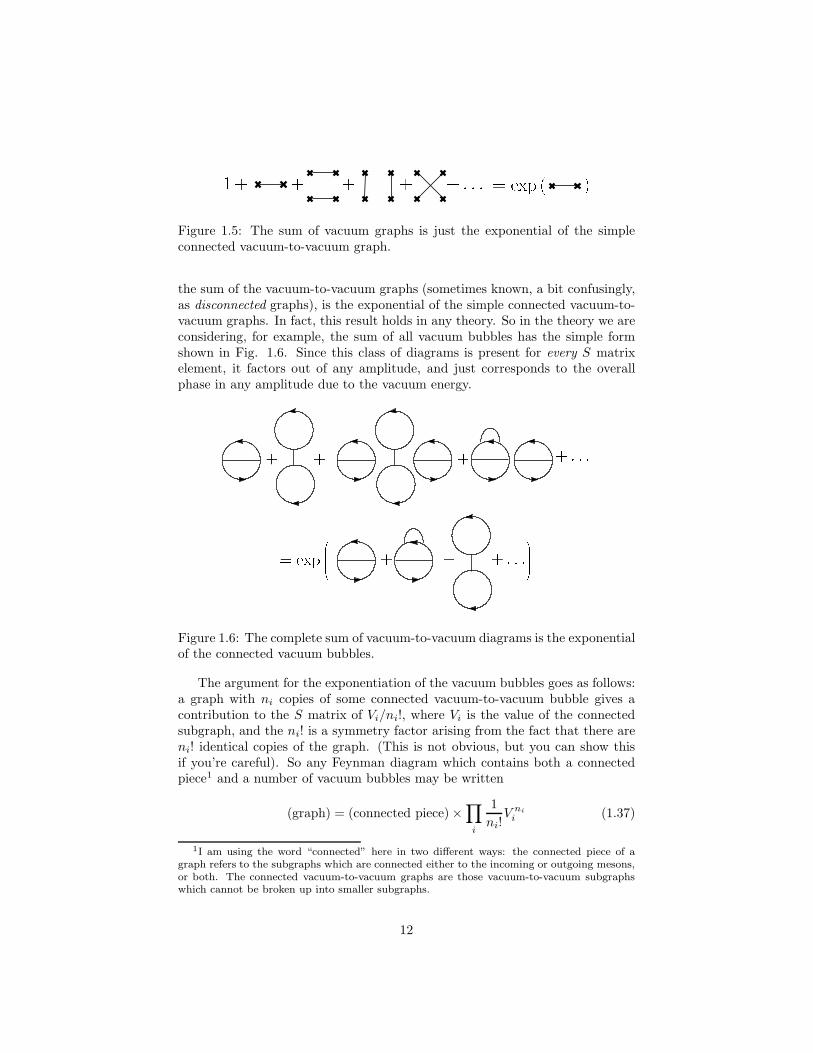
+ + : : :1+ + + = exp ( )Figure 1.5: The sum of vacuum graphs is just the exponential of the simpleconnected vacuum-to-vacuum graph.

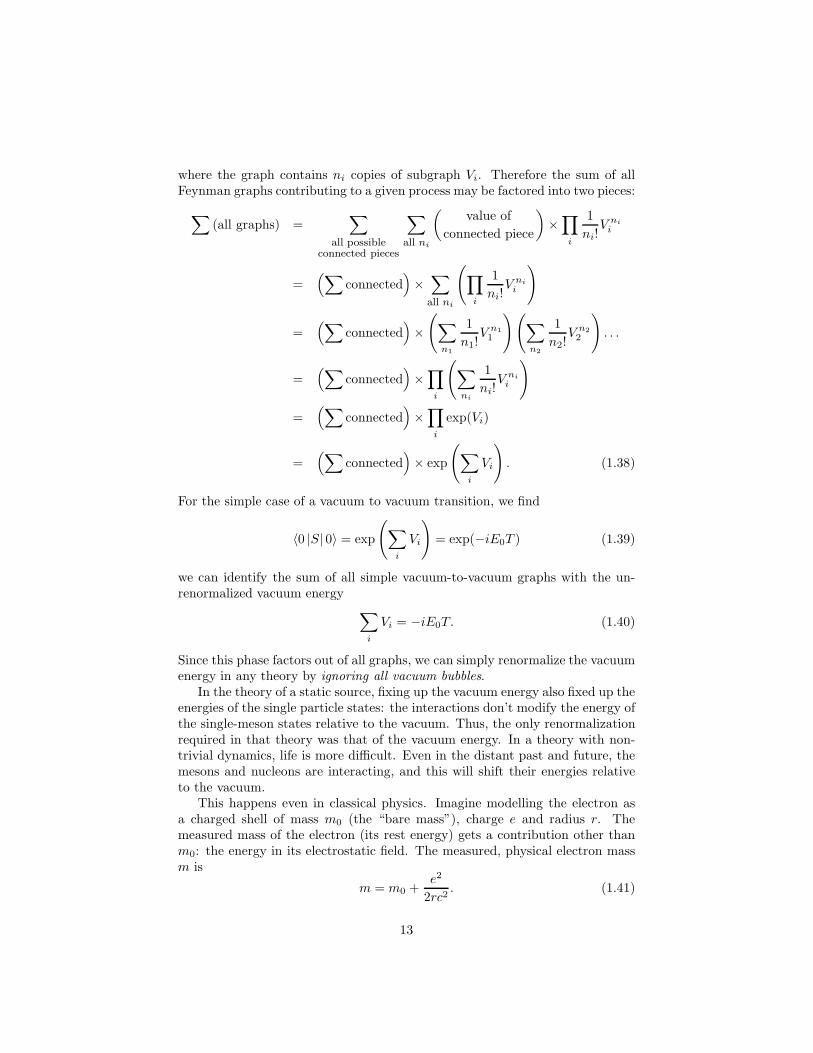
the sum of the vacuum-to-vacuum graphs (sometimes known, a bit confusingly,as disconnected graphs), is the exponential of the simple connected vacuum-to-vacuum graphs. In fact, this result holds in any theory. So in the theory we areconsidering, for example, the sum of all vacuum bubbles has the simple formshown in Fig. 1.6. Since this class of diagrams is present for every S matrixelement, it factors out of any amplitude, and just corresponds to the overallphase in any amplitude due to the vacuum energy.

= exp 0BBBB@ 1CCCCA+ + : : :+ +

++ + : : :Figure 1.6: The complete sum of vacuum-to-vacuum diagrams is the exponentialof the connected vacuum bubbles.

The argument for the exponentiation of the vacuum bubbles goes as follows:a graph with ni copies of some connected vacuum-to-vacuum bubble gives acontribution to the S matrix of Vi/ni!, where Vi is the value of the connectedsubgraph, and the ni! is a symmetry factor arising from the fact that there areni! identical copies of the graph. (This is not obvious, but you can show thisif you’re careful). So any Feynman diagram which contains both a connectedpiece1 and a number of vacuum bubbles may be written

(graph) = (connected piece) ×∏

i

1

ni!V ni

i (1.37)

1I am using the word “connected” here in two different ways: the connected piece of agraph refers to the subgraphs which are connected either to the incoming or outgoing mesons,or both. The connected vacuum-to-vacuum graphs are those vacuum-to-vacuum subgraphswhich cannot be broken up into smaller subgraphs.

12

where the graph contains ni copies of subgraph Vi. Therefore the sum of allFeynman graphs contributing to a given process may be factored into two pieces:

∑

(all graphs) =∑

all possibleconnected pieces

∑

all ni

(

value of

connected piece

)

×∏

i

1

ni!V ni

i

=(

∑

connected)

×∑

all ni

(

∏

i

1

ni!V ni

i

)

=(

∑

connected)

×(

∑

n1

1

n1!V n1

1

)(

∑

n2

1

n2!V n2

2

)

. . .

=(

∑

connected)

×∏

i

(

∑

ni

1

ni!V ni

i

)

=(

∑

connected)

×∏

i

exp(Vi)

=(

∑

connected)

× exp

(

∑

i

Vi

)

. (1.38)

For the simple case of a vacuum to vacuum transition, we find

〈0 |S| 0〉 = exp

(

∑

i

Vi

)

= exp(−iE0T ) (1.39)

we can identify the sum of all simple vacuum-to-vacuum graphs with the un-renormalized vacuum energy

∑

i

Vi = −iE0T. (1.40)

Since this phase factors out of all graphs, we can simply renormalize the vacuumenergy in any theory by ignoring all vacuum bubbles.

In the theory of a static source, fixing up the vacuum energy also fixed up theenergies of the single particle states: the interactions don’t modify the energy ofthe single-meson states relative to the vacuum. Thus, the only renormalizationrequired in that theory was that of the vacuum energy. In a theory with non-trivial dynamics, life is more difficult. Even in the distant past and future, themesons and nucleons are interacting, and this will shift their energies relativeto the vacuum.

This happens even in classical physics. Imagine modelling the electron asa charged shell of mass m0 (the “bare mass”), charge e and radius r. Themeasured mass of the electron (its rest energy) gets a contribution other thanm0: the energy in its electrostatic field. The measured, physical electron massm is

m = m0 +e2

2rc2. (1.41)

13

Note that as r → 0, the measured mass differs from the bare mass by a divergentquantity. This is just the UV divergence associated with point particles again.Since the measured mass is some finite number fixed by experiment, this meansthe bare mass must also be divergent. This puts us again in the somewhatunnerving but nevertheless necessary position of having formally divergent termsin the Lagrangian.

Once again, this is going to be bad news for scattering theory. Just as thefailure to match up the ground state energy for the noninteracting and fullHamiltonians in the previous section produced T dependent phases in 〈0 |S| 0〉,the failure to match up one particle state energies in this theory will yield Tdependent phases in 〈~k |S|~k′〉, when in fact we should have

〈~k |S|~k′〉 = δ(3)(~k − ~k′). (1.42)

Since there is nothing for a free particle to scatter off, it should just propagatefreely (along with its meson field) from t = −∞ to t = +∞. To fix this up, wewill require counterterms for the masses of both the nucleon and meson masses,

Lc.t. = a+ bψ∗ψ + cφ2 (1.43)

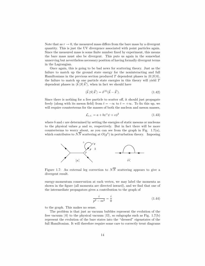
where b and c are determined by setting the energies of static mesons or nucleonsto the physical values µ and m, respectively. But in fact there will be morecounterterms to worry about, as you can see from the graph in Fig. 1.7(a),which contributes to NN scattering at O(g4) in perturbation theory. Imposingpk p p k(a) (b)Figure 1.7: An external leg correction to NN scattering appears to give adivergent result.

energy-momentum conservation at each vertex, we may label the momenta asshown in the figure (all momenta are directed inward), and we find that one ofthe intermediate propagators gives a contribution to the graph of

i

p2 −m2=i

0(1.44)

to the graph. This makes no sense.The problem is that just as vacuum bubbles represent the evolution of the

free vacuum | 0〉 to the physical vacuum |Ω〉, so subgraphs such as Fig. 1.7(b)represent the evolution of the bare states into the “dressed” eigenstates of thefull Hamiltonian. It will therefore require some care to correctly treat diagrams

14

with external leg corrections. The solution has to do with the normalization ofthe field operators themselves.

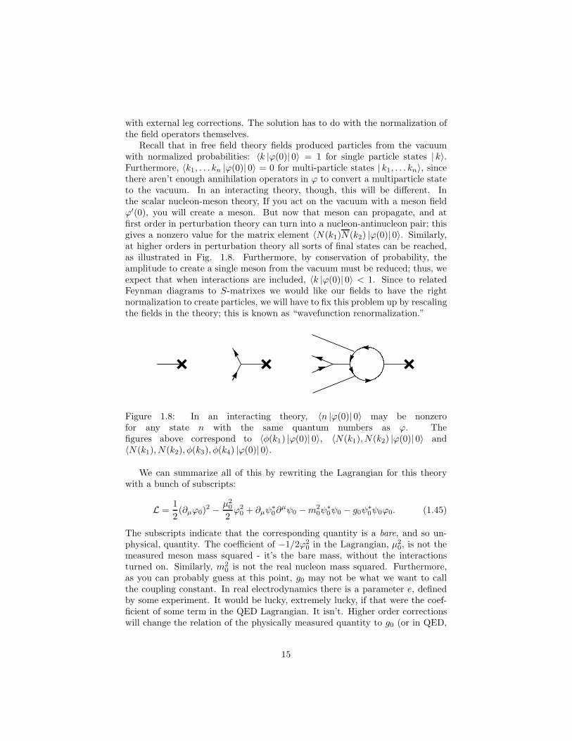
Recall that in free field theory fields produced particles from the vacuumwith normalized probabilities: 〈k |ϕ(0)| 0〉 = 1 for single particle states | k〉.Furthermore, 〈k1, . . . kn |ϕ(0)| 0〉 = 0 for multi-particle states | k1, . . . kn〉, sincethere aren’t enough annihilation operators in ϕ to convert a multiparticle stateto the vacuum. In an interacting theory, though, this will be different. Inthe scalar nucleon-meson theory, If you act on the vacuum with a meson fieldϕ′(0), you will create a meson. But now that meson can propagate, and atfirst order in perturbation theory can turn into a nucleon-antinucleon pair; thisgives a nonzero value for the matrix element 〈N(k1)N(k2) |ϕ(0)| 0〉. Similarly,at higher orders in perturbation theory all sorts of final states can be reached,as illustrated in Fig. 1.8. Furthermore, by conservation of probability, theamplitude to create a single meson from the vacuum must be reduced; thus, weexpect that when interactions are included, 〈k |ϕ(0)| 0〉 < 1. Since to relatedFeynman diagrams to S-matrixes we would like our fields to have the rightnormalization to create particles, we will have to fix this problem up by rescalingthe fields in the theory; this is known as “wavefunction renormalization.”

Figure 1.8: In an interacting theory, 〈n |ϕ(0)| 0〉 may be nonzerofor any state n with the same quantum numbers as ϕ. Thefigures above correspond to 〈φ(k1) |ϕ(0)| 0〉, 〈N(k1), N(k2) |ϕ(0)| 0〉 and〈N(k1), N(k2), φ(k3), φ(k4) |ϕ(0)| 0〉.

We can summarize all of this by rewriting the Lagrangian for this theorywith a bunch of subscripts:

L =1

2(∂µϕ0)

2 − µ20

2ϕ2

0 + ∂µψ∗0∂

µψ0 −m20ψ

∗0ψ0 − g0ψ

∗0ψ0ϕ0. (1.45)

The subscripts indicate that the corresponding quantity is a bare, and so un-physical, quantity. The coefficient of −1/2ϕ2

0 in the Lagrangian, µ20, is not the

measured meson mass squared - it’s the bare mass, without the interactionsturned on. Similarly, m2

0 is not the real nucleon mass squared. Furthermore,as you can probably guess at this point, g0 may not be what we want to callthe coupling constant. In real electrodynamics there is a parameter e, definedby some experiment. It would be lucky, extremely lucky, if that were the coef-ficient of some term in the QED Lagrangian. It isn’t. Higher order correctionswill change the relation of the physically measured quantity to g0 (or in QED,

15

e0). Finally, the field ϕ in the Lagrangian is not the one we actually want touse to create and annihilate particles. The field ϕ0 is normalized to satisfy thecanonical commutation relations,

[ϕ0(~x, t), ϕ0(~y, t)] = iδ(3)(~x− ~y) (1.46)

and in general won’t have the correct normalization to create a meson from thevacuum,

〈k |ϕ0(0)| 0〉 < 1. (1.47)

Now, at this point we can proceed in one of two ways. The two approachesdiffer in which terms of L we treat exactly, and which as perturbations.

1. We could work directly with the Lagrangian (1.45), and calculate physicalquantities from this. This is the approach used by Peskin & Schroeder inchapters 6 and 7. In this case, we would get expressions for the physicalquantities µ, m and g in terms of the bare parameters µ0, m0 and g0.All of our cross sections would also come out as functions of the bareparameters, but with a bit of work we could convert these to expressionsin terms of the physical quantities µ, m and g. The disadvantage of thisapproach is that everything is expressed in terms of unphysical (generallydivergent) quantities. Since we don’t actually care what the bare massesor couplings are, this approach is rather unwieldy, particularly at higherorders in perturbation theory.

2. A better approach (used by Peskin & Schroeder in chapter 10 and beyond),known as “renormalized perturbation theory”, is to express L in termsof the physical parameters right from the start. We therefore rewriteEq. (1.45) as

L =1

2(∂µϕ)2 − µ2

2ϕ2 + ∂µψ

∗∂µψ −m2ψ∗ψ − gψ∗ψϕϕ+ Lc.t. (1.48)

where Lc.t. is the counterterm Lagrangian

Lc.t. =A

2(∂µϕ)2 − B

2ϕ2 + C∂µψ

∗∂µψ −Dm2ψ∗ψ − Eψ∗ψϕ+ constant.

(1.49)It is a simple matter to compare Eqs. (1.45), (1.48) and (1.49) and readoff the relation between the counterterms A− E and the bare quantities:ϕ0 =

√1 +Bϕ, µ2

0 = (µ2 + C)/(1 + B), etc. The constant is just thevacuum energy counterterm. The two Lagrangians are identical; the onlydifference is that we have split up the free piece and the interacting piecedifferently. In the first approach, the meson propagator has a pole atthe bare mass µ0, as shown in Fig. 1.9(a). In the second, the mesonpropagator has a pole at the physical meson mass µ, and the countertermsgive new interactions, as shown in Fig. 1.9(b). The counterterms A − Eare determined, order by order in perturbation theory, by requiring thatthey exactly cancel the contributions to the leading order masses and

16

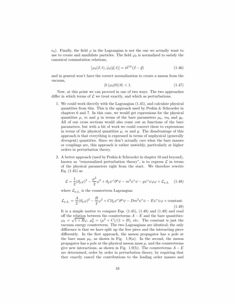
couplings due to the interactions, just as the vacuum energy countertermwas adjusted to exactly cancel the corrections to the energy of the vacuumstate. So for example, the meson mass shift produced at O(g2) by thediagram in Fig. 1.9(c) is precisely cancelled by C.2

ip2 20 ip2 2 p p p(a) (b)

(c)i(Bp2 C)

Figure 1.9: (a) In unrenormalized perturbation theory, the propagator has a poleat the bare mass µ0. (b) In renormalized perturbation theory, the pole of thepropagator is at the physical mass m; the counterterms B and C give additionalinteraction vertices. For example, at O(g2), the counterterm C precisely cancelsthe meson mass shift produced by the diagram (c).

In most instances the second approach is simpler. It allows us to avoiddealing with unphysical and uninteresting bare parameters, and deal insteaddirectly with the physical quantities.

Unfortunately, we are still stuck with the clumsy turning on and off functionf(t) we have been using as the basis of scattering theory. It has proved sufficientfor our limited purposes thus far, but it would be really nice to do away with italtogether. The real world doesn’t have a turning on and off function. Is therea way to define scattering theory without it? In the next section we will discusshow this can be done, and reformulate scattering theory in a more elegantlanguage. Then we can start calculating radiative corrections in renormalizedperturbation theory.

2This does not mean that the complete diagram (c) is cancelled by the counterterm! Thisdiagram is a function of p2, and only for p2 = m2 is it cancelled by the counterterm; at othervalues of p2 (relevant when the meson is off-shell) it contributes.

17

2 Reformulating Scattering Theory

With the last chapter as motivation, we now proceed to put scattering theory ona firmer foundation. To do that, it is useful first to think a bit about Feynmandiagrams in a somewhat more general way than we are used to. Note that thenext few subsections will be phrased in our old description of scattering theory,so we will not yet worry about the distinction between bare and full fields - wewill have that forced on us later.

2.1 Feynman Diagrams with External Lines off the Mass

Shell

Up to now, we’ve had a rather straightforward way to interpret Feynman di-agrams: with all the external lines corresponding to physical particles, theycorrespond to S matrix elements. In order to reformulate scattering theory,we will have to generalize this notion somewhat, to include Feynman diagramswhere the external legs are not necessarily on the mass shell; that is, the externalmomenta do not obey p2 = m2. Clearly, such quantities do not directly corre-spond to S matrix elements. Nevertheless, they will turn out to be extremelyuseful objects.

Let us denote the sum of all Feynman diagrams with n external lines carryingmomenta k1, . . . , kn directed inward by

G(n)(k1, . . . , kn)

as denote in the figure for n = 4. (For simplicity, we will restrict ourselvesk1 k2k3k4 ~G(4)(k1; k2; k3; k4)

Figure 2.1: The blob represents the sum of all Feynman diagrams; the momentaflowing through the external lines is unrestricted.

to Feynman diagrams in which only one type of scalar meson appears on theexternal lines. The extension to higher-spin fields is straightforward; it justclutters up the formulas with indices). The question we will answer in thissection is the following: Can we assign any meaning to this blob if the momenta

on the external lines are unrestricted, off the mass shell, and maybe not even

satisfying k1 + k2 + k3 + k4 = 0?In fact, we will give three affirmative answers to this question, each one of

which will give a bit more insight into Feynman diagrams.

18

2.1.1 Answer One: Part of a Larger Diagram

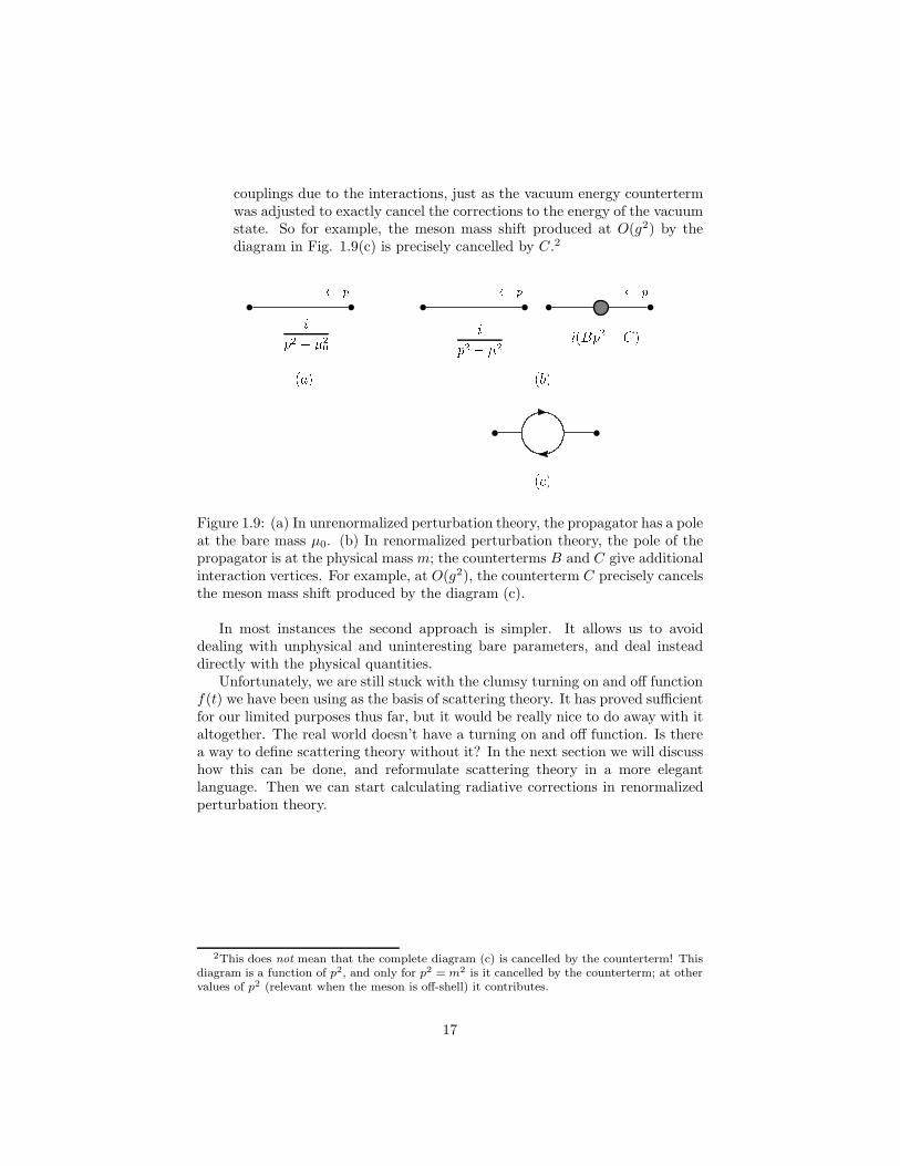
The most straightforward answer to this question is that the blob could bean internal part of a more complicated graph. Let’s say we were interested incalculating the graphs in Fig. 2.2(a-d), which all have the form shown in Fig.2.2(e), where the blob represents the sum of all graphs (at least up to someorder in perturbation theory). Recalling our discussion of Feynman diagrams

(a) (b)(c) (d) (e)

Figure 2.2: The graphs in (a-d) all have the form of (e).

with internal loops, we would label all internal lines with arbitrary momentaand integrate over them. So if we had a table of blobs, we could simply plug itinto this graph, do the appropriate integrals, and have something which we doknow how to interpret: an S-matrix element.

So this gives us a sensible, and possibly even useful, interpretation of theblob. Before we go any further, we should choose a couple of conventions.For example, we could include or not include the n propagators which hangoff G(k1, . . . , kn). We could also include or not include the overall energy-momentum conserving δ-function. We’ll include them both.

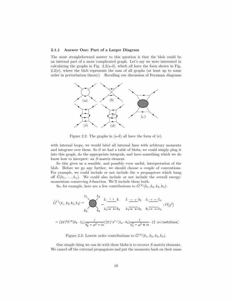
So, for example, here are a few contributions to G(4)(k1, k2, k3, k4):~G(2)(k1; k2; k3; k4) = +O(g2)= (2)4(4)(k1+k4) ik21 2 + i(2)4(4)(k2+k3) ik22 2 + i+(2 permutations)= +k1k2 k3k4 +k1k2 k3k4 k1 k2k3k4 k1k2 k3k4! ! ! ! ! ! Figure 2.3: Lowest order contributions to G(4)(k1, k2, k3, k4).

One simple thing we can do with these blobs is to recover S-matrix elements.We cancel off the external propagators and put the momenta back on their mass

19

shells. Thus, we get

〈k3, k4 |(S − 1)| k1, k2〉 =

4∏

r=1

k2r − µ2

iG(−k3,−k4, k1, k2). (2.1)

Because of the four factors of zero out front when the momenta are on theirmass shell, the graphs that we wrote out above do not contribute to S − 1,as expected (since they don’t contribute to scattering away from the forwarddirection).

2.1.2 Answer Two: The Fourier Transform of a Green Function

We have found one meaning for our blob. We can use it to obtain anotherfunction, its Fourier transform, which we can then give another meaning to.Using the convention for Fourier transforms,

f(x) =

∫

d4k

(2π)4f(k)eik·x

f(k) =

∫

d4xf(x)e−ik·x (2.2)

(again keeping with our convention that each dk comes with a factor of 1/(2π)),we have

G(n)(x1, . . . , xn) =

∫

d4k1

(2π)4. . .

∫

d4kn(2π)4

exp(ik1·x1+. . .+ikn·xn)G(n)(k1, . . . , kn)

(2.3)(hence the tilde over G defined in momentum space).

Now, consider adding a source to any given theory,

L → L + ρ(x)ϕ(x) (2.4)

where ρ(x) is a specified c-number source, not an operator. As you showed ina problem set back in the fall, this adds a new vertex to the theory, shown inFig. 1.2.

Now, consider the vacuum-to-vacuum transition amplitude, 〈0 |S| 0〉, in thismodified theory. At n’th order in ρ(x), all the contributions to 〈0 |S| 0〉 comefrom diagrams of the form shown in the figure.

Thus, the n’th order (in ρ(x)) contribution to 〈0 |S| 0〉 to all orders in g is

in

n!

∫

d4k1

(2π)4. . .

∫

d4kn(2π)4

ρ(−k1) . . . ρ(−kn) G(n)(k1, . . . , kn). (2.5)

The reason for the factor of 1/n! arises because if I treat all sources as distin-guishable, I overcount the number of diagrams by a factor of n!. Thus, to allorders, we have

〈0 |S| 0〉 = 1 +∞∑

n=1

in

n!

∫

d4k1

(2π)4. . .

∫

d4kn(2π)4

ρ(−k1) . . . ρ(−kn) G(n)(k1, . . . , kn)

20

k1k2 k3k4 k5kn

Figure 2.4: n’th order contribution to 〈0 |S| 0〉 in the presence of a source.

= 1 +∞∑

n=1

in

n!

∫

d4x1 . . . d4xn ρ(x1) . . . ρ(xn)G(n)(x1, . . . , xn). (2.6)

This provides us with the second answer to our question. The Fourier transformof the sum of Feynman diagrams with n external lines off the mass shell is aGreen function (that’s what the G stands for). Recall we already introduced then = 2 Green function (in free field theory) in connection with the exact solutionto free field theory with a source.

Let’s explicitly note that the vacuum-to-vacuum transition ampitude de-pends on ρ(x) by writing it as

〈0 |S| 0〉ρ.〈0 |S| 0〉ρ is a functional of ρ, which is how mathematicians denote functions offunctions. Really, it is just a function of an infinite number of variables, thevalue of the source at each spacetime point. It comes up often enough that itgets a name,

Z[ρ] = 〈0 |S| 0〉ρ. (2.7)

(The square bracket reminds you that this is a function of the function ρ(x).)Z[ρ] is called the generating functional for the Green function because, in theinfinite dimensional generalization of a Taylor series, we have

δnZ[ρ]

δρ(x1) . . . δρ(xn)

∣

∣

∣

∣

= inG(n)(x1, . . . , xn) (2.8)

where the δ instead of δ once again reminds you that we are dealing with func-tionals here: you are taking a partial derivatives of Z with respect to ρ(x),holding a 4 dimensional continuum of other variable fixed. This is called a func-

tional derivative. As discussed in Peskin & Schroeder, p. 298, the functionalderivative obeys the basic axiom (in four dimensions)

δ

δJ(x)J(y) = δ(4)(x − y), or

δ

δJ(x)

∫

d4y J(y)ϕ(y) = ϕ(x). (2.9)

This is the natural generalization, to continuous functions, of the rule for discrete

21

vectors,∂

∂xixj = δij , or

∂

∂xi

∑

j

xjkj = ki. (2.10)

The generating functional Z[J ] will be particularly useful when we study thepath integral formulation of QFT.

The term “generating functional” arises in analogy with the functions of twovariables, which when you Taylor expand in one variable, the coefficients area set of functions of the other. For example, the generating function for theLegendre polynomials is

f(x, z) =1√

z2 − 2xz + 1(2.11)

since when expanded in z, the coefficients of zn is the Legendre polynomialPn(x):

f(x, z) = 1 + xz +1

2(3x2 − 1)z2 + . . .

= P0(x) + zP1(x) + z2P2(x) + . . . . (2.12)

Similarly, when Z[ρ] in expanded in powers of ρ(x), the coefficient of ρn isproportional to the n-point Green function G(n)(x1, . . . , xn). Thus, all Greenfunctions, and hence all S matrix elements (and so all physical information aboutthe system) are encoded in the vacuum persistance amplitude in the presenceof an external source ρ.

2.1.3 Answer Three: The VEV of a String of Heisenberg Fields

But wait, there’s more. Once again, let us consider adding a source term to thetheory. Thus, the Hamiltonian may be written

H0 + HI → H0 + HI − ρ(x)ϕ(x) (2.13)

where H0 is the free-field piece of the Hamiltonian, and HI contains the in-teractions. Now, as far as Dyson’s formula is concerned, you can break theHamiltonian up into a “free” and interacting part in any way you please. Let’stake the “free” part to be H0 + HI and the interaction to be ρϕ. I put quotesaround “free”, because in this new interaction picture, the fields evolve accord-ing to

ϕ(~x, t) = eiHtϕ(~x, 0)e−iHt (2.14)

where H =∫

d3xH0+HI . These fields aren’t free: they don’t obey the free fieldequations of motion. You can’t define a contraction for these fields, and thusyou can’t do Wick’s theorem. They are what we would have called Heisenbergfields if there had been no source, and so we will subscript them with an H .

22

Now, just from Dyson’s formula, we find

Z[ρ] = 〈0 |S| 0〉ρ = 〈0 |T exp

(

i

∫

d4xρ(x)ϕH(x)

)

| 0〉 (2.15)

= 1 +

∞∑

n=1

in

n!

∫

d4x1 . . . d4xn ρ(x1) . . . ρ(xn)〈0 |T (ϕH(x1) . . . ϕH(xn)) | 0〉

and so we clearly have

G(n)(x1, . . . , xn) = 〈0 |T (ϕH(x1) . . . ϕH(xn)) | 0〉. (2.16)

For n = 2, we have the two-point Green function 〈0 |T (ϕH(x1)ϕH(x2)) | 0〉.This looks like our definition of the propagator, but it’s not quite the samething. The Feynman propagator was defined as a Green function for the free

field theory; the two-point Green function is defined in the interacting theory.One of the tasks of the next few sections is to see how these are related.

2.2 Green Functions and Feynman Diagrams

From the discussion in the previous section, we have three logically distinctobjects:

1. S-matrix elements (the physical observables we wish to measure),

2. the sum of Feynman diagrams (the things we know how to calculate), and

3. n-point Green functions, defined via by Eq. (2.8) or (2.16).

By introducing a turning on and off function, we could show that these were allrelated. Now we want to get rid of that crutch, and define perturbation theoryin a more sensible way. The question we will then have to address is, what isthe relation between these objects in our new formulation of scattering theory?

We set up the problem as follows. Imagine you have a well-defined theory,with a time independent Hamiltonian H (the turning on and off function isgone for good) whose spectrum is bounded below, whose lowest lying state isnot part of a continuum (i.e. no massless particles yet), and the Hamiltonianhas actually been adjusted so that this state, |Ω〉, the physical vacuum, satisfies

H |Ω〉 = 0. (2.17)

The vacuum is translationally invariant and normalized to one

~P |Ω〉 = 0, 〈Ω |Ω〉 = 1. (2.18)

Now, let H → H− ρ(x)ϕ(x) and define

Z[ρ] ≡ 〈Ω |S|Ω〉ρ= 〈Ω |U(∞,−∞)|Ω〉ρ (2.19)

23

where the ρ subscript again means, in the presence of a source ρ(x), and theevolution operator U(t1, t2) is the Schorodinger picture evolution operator forthe Hamiltonian

∫

d3x (H− ρ(x)ϕ(x)). We then define

G(n)(x1, . . . , xn) =1

inδnZ[ρ]

δρ(x1) . . . δρ(xn). (2.20)

Note that this is, at least in principle, different from our previous definitions of ZandG, which implicitly referred to S matrix elements taken between free vacuumstates, with the interactions defined with the turning on and off function. Thus,we can ask two questions:

1. Is G(n) defined this way the Fourier transform of the sum of all Feynman

graphs? Let’s call the G(n) defined as the sum of all Feynman graphs G(n)F

and the Z which generates these ZF . The question then is, is G(n) = G(n)F ?

Or equivalently, is Z = ZF ?

The answer, fortunately, will be “yes”. In other words, we can computeGreen functions just as we always did, as the sum of Feynman graphs.This is actually rather surprising, since we derived Feynman rules basedon the action of interacting fields on the bare vacuum, not the full vacuum.

2. Are S matrix elements obtained from Green functions in the same way asbefore? For example, is

〈k′1, k′2 |S − 1| k1, k2〉 =∏

a

k2a − µ2

iG(−k′1,−k′2, k1, k2)? (2.21)

The answer will be, “almost.” The problem will be, as we have alreadydiscussed, that in an interacting theory, the bare field ϕ0(x) no longercreates mesons with unit probability. The formula will hold, but onlywhen the Green function G is defined using renormalized fields ϕ insteadof bare fields.

First we will answer the first question: Is G(n) = G(n)F ?3 Our answer will

be similar to the derivation of Wick’s theorem on pages 82-87 of Peskin &Schroeder, which you should look at as well.

First of all, using Dyson’s formula just as we did at the end of the lastsection, it is easy to show that

G(n)(x1, . . . , xn) = 〈Ω |T (ϕH(x1) . . . ϕH(xn)) |Ω〉. (2.22)

Now let’s show that this is what we get by blindly summing Feynman diagrams.The object which had a graphical expansion in terms of Feynman diagrams

was

ZF [ρ] = limt±→±∞

〈0 |T exp

(

−i∫ t+

t−

[HI − ρ(x)ϕI (x)]

)

| 0〉 (2.23)

3Since the answer to this question doesn’t depend on using bare fields ϕ0 or renormalizedfields ϕ, we will neglect this distinction in the following discussion.

24

where I remind you that | 0〉 refers to the bare vacuum, satisfying H0| 0〉 = 0.Now, we know that we will have to adjust the constant part of HI with avacuum energy counterterm to eliminate the vacuum bubble graphs when ρ = 0.Equivalently, since as argued in the previous chapter the sum of vacuum bubblesis universal, an easier way to get rid of them is simply to divide by 〈0 |S| 0〉; thisgives

ZF [ρ] = limt±→±∞

〈0 |T exp(

−i∫ t+t−

[HI − ρ(x)ϕI(x)])

| 0〉

〈0 |T exp(

−i∫ t+t−

HI

)

| 0〉. (2.24)

To get G(n)F (x1, . . . , xn), we do n functional derivatives with respect to ρ and

then set ρ = 0:

G(n)F (x1, . . . , xn) = lim

t±→±∞

〈0 |T[

ϕI(x1) . . . ϕI(xn) exp(

−i∫ t+t−

[HI − ρϕI ])]

| 0〉

〈0 |T exp(

−i∫ t+t−

HI

)

| 0〉.

(2.25)Now, we have to show that this is equal to Eq. (2.22). This will take a bit ofwork.

First of all, since Eq. (2.25) is manifestly symmetric under permutations ofthe xi’s, we can simply prove the equality for a particularly convenient timeordering. So let’s take

t1 > t2 > . . . > tn (2.26)

In this case, we can drop the T -ordering symbol from G(n)(x1, . . . , xn). Now,since

UI(tb, ta) = T exp

(

−i∫ tb

ta

d4xHI

)

(2.27)

is the usual time evolution operator, we can express the time ordering in G(n)F

as

G(n)F (x1, . . . , xn) = lim

t±→±∞

〈0 |UI(t+, t1)ϕI(x1)UI(t1, t2)ϕI(x2) . . . ϕI(xn)UI(tn, t−)| 0〉〈0 |UI(t+, t−)| 0〉 .

(2.28)Now, everywhere that UI(ta, tb) appears, rewrite it as UI(ta, 0)UI(0, tb), andthen use the relation between Heisenberg and Interaction fields,

ϕH(xi) = UI(ti, 0)†ϕI(xi)UI(ti, 0)

= UI(0, ti)ϕI(xi)UI(ti, 0) (2.29)

to convert everything to Heisenberg fields, and get rid of those intermediate U ’s:

G(n)F (x1, . . . , xn) = lim

t±→±∞

〈0 |UI(t+, 0)ϕH(x1)ϕH(x2) . . . ϕH(xn)UI(0, t−)| 0〉〈0 |UI(t+, 0)UI(0, t−)| 0〉 .

(2.30)

25

Let’s concentrate on the right hand end of the expression, UI(0, t−)| 0〉 (in boththe numerator and denominator), and refer to the mess to the left of it as somefixed state 〈Ψ |. First of all, since H0| 0〉 = 0, we can trivially convert theevolution operator to the Schrodinger picture,

limt−→∞

〈Ψ |UI(0, t−)| 0〉 = limt−→∞

〈Ψ |UI(0, t−) exp(iH0t−)| 0〉 = limt−→∞

〈Ψ |U(0, t−)| 0〉.(2.31)

Next, insert a complete set of eigenstates of the full Hamiltonian, H ,

limt−→∞

〈Ψ |U(0, t−)| 0〉 = limt−→∞

〈Ψ |U(0, t−)

|Ω〉〈Ω | +∑

n6=0

|n〉〈n |

| 0〉

= 〈Ψ|Ω〉〈Ω |0〉 + limt−→−∞

∑

n6=0

eiEnt−〈Ψ|n〉〈n| 0〉 (2.32)

where the sum is over all eigenstates of the full Hamiltonian except the vacuum,and we have used the fact that H |Ω〉 = 0 and H |n〉 = En|n〉, where the En’sare the energies of the excited states.

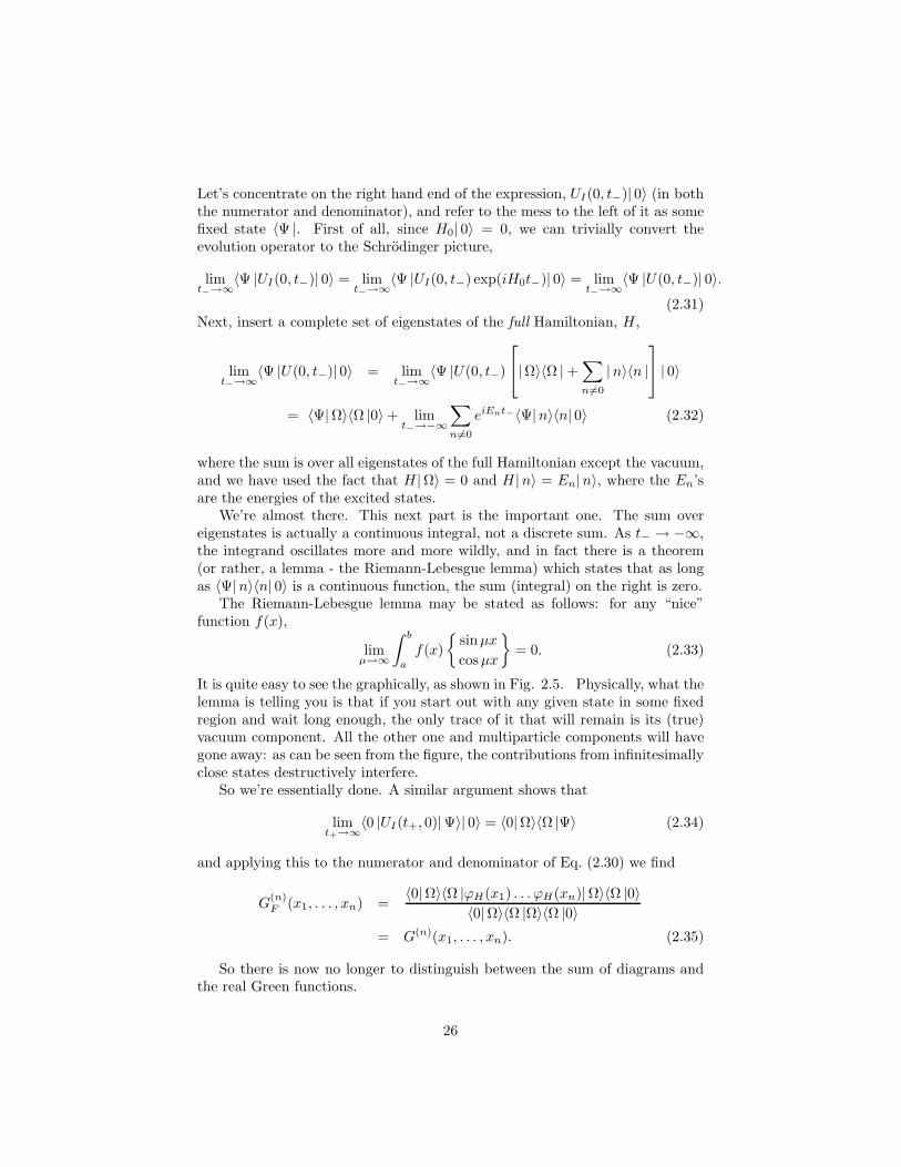
We’re almost there. This next part is the important one. The sum overeigenstates is actually a continuous integral, not a discrete sum. As t− → −∞,the integrand oscillates more and more wildly, and in fact there is a theorem(or rather, a lemma - the Riemann-Lebesgue lemma) which states that as longas 〈Ψ|n〉〈n| 0〉 is a continuous function, the sum (integral) on the right is zero.

The Riemann-Lebesgue lemma may be stated as follows: for any “nice”function f(x),

limµ→∞

∫ b

a

f(x)

sinµx

cosµx

= 0. (2.33)

It is quite easy to see the graphically, as shown in Fig. 2.5. Physically, what thelemma is telling you is that if you start out with any given state in some fixedregion and wait long enough, the only trace of it that will remain is its (true)vacuum component. All the other one and multiparticle components will havegone away: as can be seen from the figure, the contributions from infinitesimallyclose states destructively interfere.

So we’re essentially done. A similar argument shows that

limt+→∞

〈0 |UI(t+, 0)|Ψ〉| 0〉 = 〈0|Ω〉〈Ω |Ψ〉 (2.34)

and applying this to the numerator and denominator of Eq. (2.30) we find

G(n)F (x1, . . . , xn) =

〈0|Ω〉〈Ω |ϕH(x1) . . . ϕH(xn)|Ω〉〈Ω |0〉〈0|Ω〉〈Ω |Ω〉〈Ω |0〉

= G(n)(x1, . . . , xn). (2.35)

So there is now no longer to distinguish between the sum of diagrams andthe real Green functions.

26

0 0.2 0.4 0.6 0.8 1-10

-5

0

5

10 f (x)f (x) sinx

Figure 2.5: The Riemann-Lebesgue lemma: f(x) multiplied by a rapidly oscil-lating function integrates to zero in the limit that the frequency of oscillationbecomes infinite.

2.3 The LSZ Reduction Formula

We now turn to the second question: Are S matrix elements obtained fromGreen’s functions in the same way as before?

By introducing a turning on and off function, we were able to show that

〈l1, . . . , ls |S − 1| k1, . . . , kr〉 =s∏

a=1

l2a − µ2

i

r∏

b=1

k2b − µ2

iG(r+s)(−l1, . . . ,−ls, k1, . . . , kr). (2.36)

The real world does not have a turning on and off function. Is this formulacorrect? The answer is “almost.”

The correct relation between S matrix elements (what we want) and Greenfunctions (what, as we just showed, we get from Feynman diagrams) which wewill derive is called the LSZ reduction formula. Since its derivation doesn’t re-quire resorting to perturbation theory, we no longer need to make any referenceto free Hamiltonia, bare vacua, interaction picture fields, etc. So FROM NOWON all fields will be in the Heisenberg representation (no more interaction pic-ture), and states will refer to eigenstates of the full Hamiltonian (although forthe rest of this section we will continue to denote the vacuum by |Ω〉 to avoidconfusion)

ϕ(x) ≡ ϕH(x), | 0〉 ≡ |Ω〉. (2.37)

The physical one-meson states in the theory are now the complete one mesonstates, relativistically normalized

H | k〉 =

√

~k2 + µ2| k〉 ≡ ωk| k〉, 〈k′ |k〉 = (2π)32ωkδ(3)(~k − ~k′). (2.38)

27

We have actually been a bit cavalier with notation in this chapter; the fieldswe have been discussion have actually been the bare fields ϕ0 which we discussedat the end of the last chapter. Thus, we have really been talking about bare

Green functions, which we will now denote G0(n):

G(n)0 (x1, . . . , xn) = T 〈Ω |ϕ0(x1) . . . ϕ0(xn)|Ω〉. (2.39)

The reason the answer to our question is “almost” is because the bare field ϕ0

which does not have quite the right properties to create and annihilate mesons.In particular, it is not normalized to create a one particle state from the vacuumwith a standard amplitude - instead, it is normalized to obey the canonical com-mutation relations. For free field theory, these two properties were equivalent.For interacting fields, however, where the amplitude to create a meson fromthe vacuum has higher order perturbative corrections, these two properties areincompatible, as we have discussed. Furthermore, in an interacting theory ϕ0

may also develop a vacuum expectation value, 〈Ω |ϕ(x)|Ω〉 6= 0.We correct for these problems by defining a renormalized field, ϕ(x), in terms

of ϕ0. By translational invariance,

〈k |ϕ(x)|Ω〉 = 〈k |eiP ·xϕ(0)e−iP ·x|Ω〉 = eik·x〈k |ϕ(0)|Ω〉. (2.40)

By Lorentz invariance, you can see that 〈k |ϕ(0)|Ω〉 is independent of k. It issome number, which for historical reasons is denoted Z1/2 (and traditionallycalled the “wave function renormalization”), and only in free field theory will itequal 1,

Z1/2 ≡ 〈k |ϕ(0)|Ω〉. (2.41)

We now can define a new field, ϕ, which is normalized to have a standardamplitude to create one meson, and a vanishing VEV (vacuum expectationvalue)

ϕ(x) ≡ Z1/2 (ϕ0(x) − 〈Ω |ϕ0(0)|Ω〉)〈Ω |ϕ(0)|Ω〉 = 0, 〈k |ϕ(x)|Ω〉 = eik·x. (2.42)

We can now state the LSZ (Lehmann-Symanzik-Zimmermann) reduction for-mula: Define the renormalized Green functions G(n),

G(n)(x1, . . . , xn) ≡ 〈Ω |T (ϕ(x1) . . . ϕ(xn)) |Ω〉 (2.43)

and their Fourier transforms, G(n). In terms of renormalized Green functions,S matrix elements are given by

〈l1, . . . , ls |S − 1| k1, . . . , kr〉

=

s∏

a=1

l2a − µ2

i

r∏

b=1

k2b − µ2

iG(r+s)(−l1, . . . ,−ls, k1, . . . , kr) (2.44)

28

That’s it - almost, but not quite, what we had before. The only differenceis that the S matrix is related to Green functions of the renormalized fields - inour new notation, the factors of G in Eq. (2.1) should be G0. Given that it is theϕ which create normalized meson states from the vacuum, this is perhaps notso surprising. What is more surprising is that even the renormalized field ϕ(x)creates a whole spectrum of multiparticle states from the vacuum as well, andthat these do not pollute the relation between Green functions and S-matrixelements. Naıvely, you might think that the Green function would be relatedto a sum of S-matrix elements, for all different incoming multiparticle statescreated by ϕ(x). However, as we shall show, these additional states can all bearranged to oscillate away via the Riemann-Lebesgue lemma, much as in thelast section.

2.3.1 Proof of the LSZ Reduction Formula

The proof can be broken up into three parts. In the first part, I will show youhow to construct localized wave packets. The wave packet will have multiparticleas well as single particle components; however, the multiparticle components willbe set up to oscillate away after a long time. In the second part of the proof, Iwill wave my hands vigorously and discuss the creation of multiparticle statesin which the particles are well separated in the far past or future; these will becalled in and out states, and we will find a simple expression for the S matrixin terms of the operators which create wave packets. In the third part of theproof, we massage this expression and take the limit in which the wave packetsare plane waves, to derive the LSZ formula.

1. How to make a wave packet

Let us define a wave packet | f〉 as follows:

| f〉 =

∫

d3k

(2π)32ωkF (~k)| k〉 (2.45)

where F (~k) = 〈k |f〉 is the momentum space wave function of | f〉. Associatewith each F a position space function, satisfying the Klein-Gordon equationwith negative frequency,

f(x) ≡∫

d3k

(2π)32ωkF (~k)e−ik·x, k0 = ωk, (2 + µ2)f(x) = 0. (2.46)

Note that as we approach plane wave states, | v〉 → | k〉, f(x) → e−ik·x.Now, define the following odd-looking operator which is only a function of

the time, t (recall again that we are working in the Heisenberg representation,so the operators carry the time dependence)

ϕf (t) ≡ i

∫

d3x (ϕ(~x, t)∂0f(~x, t) − f(~x, t)∂0ϕ(~x, t)) . (2.47)

29

This is precisely the operator which makes single particle wave packets. Firstof all, it trivially satisfies

〈Ω |ϕf (t)|Ω〉 = 0 (2.48)

and has the correct amplitude to produce a single particle state | f〉:

〈k |ϕf (t)|Ω〉

= i

∫

d3x

∫

d3k′

(2π)22ωk′F (~k′) 〈k |

(

ϕ(x)∂0e−ik′·x − e−ik

′·x∂0ϕ(x))

|Ω〉

= i

∫

d3x

∫

d3k′

(2π)22ωk′F (~k′)

(

−iωk′e−ik′·x − e−ik

′·x∂0

)

〈k |ϕ(x)|Ω〉

= i

∫

d3k′

(2π)22ωk′F (~k′)(−iωk′ − iωk)

∫

d3x ei(~k′−~k)·~xe−i(ωk′−ωk)t

= F (~k) (2.49)

where we have used∫

d3x ei(~k′−~k)·~x = (2π)δ(3)(~k − ~k′) (2.50)

and we note that the phase factor e−i(ωk′−ωk)t becomes one once the δ functionconstraint is imposed (this will change when we consider multiparticle states).Note that this result is independent of time.

A similar derivation, with one crucial minus sign difference (so that thefactors of ωk and ωk′ cancel instead of adding), yields

〈Ω |ϕf (t)k〉 = 0. (2.51)

Thus, as far as the zero and single particle states are concerned, ϕf (t) behaves asa creation operator for wave packets. Now we will see that in the limit t→ ±∞all the other states created by ϕf (t) oscillate away.

Consider the multiparticle state |n〉, which is an eigenvalue of the momentumoperator:

Pµ|n〉 = pµn|n〉. (2.52)

Proceeding much as before, let us calculate the amplitude for ϕf (t) to make thisstate from the vacuum:

〈n |ϕf (t)|Ω〉

= i

∫

d3x

∫

d3k′

(2π)22ωk′F (~k′) 〈n |

(

ϕ(x)∂0e−ik′·x − e−ik

′·x∂0ϕ(x))

|Ω〉

= i

∫

d3x

∫

d3k′

(2π)22ωk′F (~k′)

(

−iωk′e−ik′·x − e−ik

′·x∂0

)

〈n |ϕ(x)|Ω〉

= i

∫

d3x

∫

d3k′

(2π)22ωk′F (~k′)

(

−iωk′e−ik′·x − e−ik

′·x∂0

)

eipn·x〈n |ϕ(0)|Ω〉

= i

∫

d3k′

(2π)22ωk′F (~k′)(−iωk′ − ip0

n)

∫

d3x ei(~k′−~pn)·~xe−i(ωk′−p0n)t〈n |ϕ(0)|Ω〉

30

=ωpn

+ p0n

2ωpn

F (~pn)e−i(ωpn−p0n)t〈n |ϕ(0)|Ω〉 (2.53)

whereωpn

=√

~p2n + µ2. (2.54)

Note that we haven’t had to use any information about 〈n |ϕ(x)|Ω〉 beyond thatgiven by Lorentz invariance; thus, we haven’t had to know anything about theamplitude to create multiparticle states from the vacuum. The crucial point isthe existence of the phase factor e−i(ωpn−p0n)t in Eq. (2.53), and the observationthat for a multiparticle state with a finite mass,

ωpn< p0

n. (2.55)

This should be easy to convince yourself of: a two particle state, for example,can have ~p = 0 if the particles are moving back-to-back, while the energy of thestate p0

n can vary between 2µ and ∞. In contrast, a single particle state with~p = 0 can only have p0 = ωp = µ < p0

n. Thus, for the single particle state theoscillating phase vanishes, as already shown, whereas it can never vanish formultiparticle states.

So now we have the familiar Riemann-Lebesgue argument: take some fixedstate |ψ〉, and consider 〈ψ |ϕf (t)|Ω〉 as t → ±∞. Inserting a complete set ofstates, we find

limt→±∞

〈ψ |ϕf (t)|Ω〉 = limt→±∞

〈ψ|Ω〉〈Ω |ϕf (t)|Ω〉

+

∫

d3k

(2π)32ωk〈ψ |k〉〈k |ϕf (t)|Ω〉 +

∑

n6=0,1

〈ψ |n〉〈n |ϕf (t)|Ω〉

= 〈ψ| f〉 + 0 (2.56)

where we have used the fact that the multiparticle sum vanishes by the Riemann-Lebesgue lemma.

Similarly, one can show that

limt→±∞

〈Ω |ϕf (t)|ψ〉 = 0 (2.57)

for any fixed state |ψ〉.Thus, our cunning choice of ϕf (t) was arranged so that the oscillating phases

cancelled only for the single particle state, so that only these states survivedafter infinite time. We have a similar interpretation as before: in the t → −∞limit, ϕf (t) acts on the true vacuum and creates states with one, two, ... nparticles. Taking the inner product of this state with any fixed state, we findthat at t = 0 the only surviving components are the single-particle states, whichmake up a localized wave packet.

31

2. How to make widely separated wave packets

The results of the last section were rigorous (or at least, could be made sowithout a lot of work). By contrast, in this section we will wave our handsviolently and rely on physical arguments.

We now wish to construct multiparticle states of interest to scattering prob-lems, that is, states which in the far past or far future look like well separatedwavepackets. The physical picture we will rely upon is that if F1(~k) and F2(~k)do not have common support, in the distant past and future they correspond towidely separated wave packets. Then when ϕf2(t) acts on a state in the far pastor future, it shouldn’t matter if this state is the vacuum state or the state | f1〉,since the first wavepacket is arbitrarily far away. Let us denote states createdby the action of ϕf2(t) on | f1〉 in the distant past as “in” states, and statescreated by the action of ϕf2(t) on | f1〉 in the far future as “out” states. Thenwe have

limt→∞ (−∞)

〈ψ |ϕf2(t2)| f1〉 = | f1, f2〉out (in). (2.58)

Now by definition, the S matrix is just the inner product of a given “in”state with another given “out” state,

out〈f3, f4 |f1, f2〉in = 〈f3, f4 |S| f1, f2〉. (2.59)

Thus, we have shown that

〈f3, f4 |S| f1, f2〉 = limt4→∞

limt3→∞

limt2→−∞

limt1→−∞

〈Ω |ϕf4†(t4)ϕf3†(t3)ϕf2 (t2)ϕf1 (t1)|Ω〉. (2.60)

3. Massaging the resulting expression

In principle, we have achieved our goal in Eq. (2.60): we have written anexpression for S matrix elements in terms of a weighted integral over vacuumexpectation values of Heisenberg fields. However, it doesn’t look much like theLSZ reduction formula yet, but we can do that with a bit of massaging.

What we will show is the following

〈f3, f4 |S − 1| f1, f2〉 =

∫

d4x1 . . . d4xn f

∗4 (x4)f

∗3 (x3)f2(x2)f1(x1)

× i4∏

r

(2r + µ2)〈Ω |Tϕ(x1) . . . ϕ(x4)|Ω〉. (2.61)

This looks messy and unfamiliar, but it’s not. If we take the limit in which thewave packets become plane wave states, | fi〉 → | ki〉, fi(x) → eiki·xi, we have

〈k3, k4 |S − 1| k1, k2〉 =

∫

d4x1 . . . d4xn e

ik3·x3+ik4·x4−ik2·x2−ik1·x1

×i4∏

r

(2r + µ2)G(4)(x1, . . . , x4)

32

=∏

r

k2r − µ2

iG(4)(k1, k2,−k3,−k4), (2.62)

which is precisely the LSZ formula. Note that we have taken the plane wavelimit after taking the limit in which the limit t → ±∞ required to define thein and out states; thus, in this order of limits even the plane wave in and outstates are widely separated.

Before showing this, let us prove a useful result: for an arbitrary interactingfield A and function f(x) satisfying the Klein-Gordon equation and vanishingas |x| → ∞,

i

∫

d4x f(x)(2 + µ2)A(x) = i

∫

d4x f(x)∂20A(x) +A(x)(−∇2 + µ2)f(x)

= i

∫

d4x f(x)∂20A(x) −A(x)∂2

0f(x)

=

∫

dt ∂0

∫

d3x i (f(x)∂0A(x) −A(x)∂0f(x))

= −∫

dt ∂0Af (t)

=

(

limt→−∞

− limt→+∞

)

Af (t) (2.63)

where we have integrated once by parts, and Af (t) is defined as in Eq. (2.47).Similarly, we can show

i

∫

d4x f∗(x)(2 + µ2)A(x) =

(

limt→+∞

− limt→−∞

)

Af†(t). (2.64)

Note the difference in the signs of the limits. We can now use these relations toconvert factors of (2 + µ2)ϕ(x) to ϕf (t) on the RHS of Eq. (2.61). Doing thisfor each of the xi’s, we obtain

RHS =

(

limt4→+∞

− limt4→−∞

)(

limt3→+∞

− limt3→−∞

)(

limt2→−∞

− limt2→+∞

)

×(

limt1→−∞

− limt1→+∞

)

〈Ω |Tϕf1(x1)ϕf2(x2)ϕ

f3†(x3)ϕf4†(x4)|Ω〉.

(2.65)

Now we can evaluate the limits one by one.First of all, when t4 → −∞, it is the earliest (in the order of limits which

we have taken), and so acts on the vacuum. Thus, according to the complexconjugate of Eq. (2.57), we get zero. When t4 → +∞, it is the latest, and actson the vacuum state on the left, to give 〈f4 |. Similarly, only the t3 → ∞ limit

contributes, creating the state out〈f3, f4 |. Next, taking the two limits of t2, wefind

RHS =

(

limt1→−∞

− limt1→+∞

)(

out〈f3, f4 |ϕf1(t1)| f2〉

33

− limt2→+∞

out〈f3, f4 |ϕf2(t2)ϕf1(t1)|Ω〉)

. (2.66)

Unfortunately, we don’t know how ϕf2(t2 → ∞) acts on a multi-meson outstate, and so it’s not clear what the second term is. Let’s parameterize ourignorance and define

〈ψ | ≡ limt2→∞

out〈f3, f4 |ϕf2(t2). (2.67)

Then taking the t1 limits, we find

RHS = out〈f3, f4 |f1, f2〉in − out〈f3, f4 |f1, f2〉out − 〈ψ |f1〉 + 〈ψ |f1〉= 〈f3, f4 |S − 1| f1, f2〉 (2.68)

as required. Note that we have used the fact (from Eq. (2.56)) that

limt1→∞

〈ψ |ϕf1 (t1)|Ω〉 = limt1→−∞

〈ψ |ϕf1(t1)|Ω〉 = 〈ψ |f1〉. (2.69)

So that’s it - we’ve proved the reduction formula. It was a bit involved, butthere are a few important things to remember:

1. The proof relied only on the properties

〈Ω |ϕ(0)|Ω〉 = 0, 〈k |ϕ(0)|Ω〉 = 1. (2.70)

No other properties of ϕ were assumed. In particular, ϕ was not assumedto have any particular relation to the bare field ϕ0 which appears in theLagrangian - the simplest relation is Eq. (2.42), but the Green functionsof any field ϕ which satisfies the requirements (2.70) will give the correctS-matrix elements. For example,

ϕ(x) = ϕ(x) + 12gϕ(x)2 (2.71)

is a perfectly good field to use in the reduction formula.

Physically, this is again because of the Riemann-Lebesgue destructive in-terference. One appropriately renormalized, ϕ(0) and ϕ(0) only differ intheir vacuum to multiparticle state matrix elements. But this differencejust oscillates away - the multiparticle states created by the field are irrel-evant.

Practically, this has a very useful consequence: you can always make anonlinear field redefinition for any field in a Lagrangian, and it doesn’tchange the value of S-matrix elements (although it will change the Greenfunctions off shell, but that is irrelevant to the physics). In some casesthis is quite convenient, since some complicated nonrenormalizable La-grangians may take particularly simple forms after an appropriate fieldredefinition. A simple example of this is given on the first problem set.

34

This is a good result to remember, if only to save a few trees. A lot ofpapers have been written (even in the past few years) which claim thatsome particular field is the “correct” one to use in a given problem. Mostof these papers are idiotic - the authors’ pet form of the Lagrangian hasbeen obtained by a simple nonlinear field redefinition from the standardform, and so is guaranteed to give the same physics.

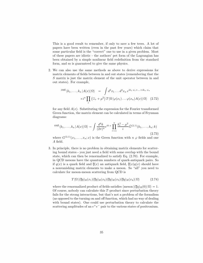
2. We can also use the same methods as above to derive expressions formatrix elements of fields between in and out states (remembering that theS matrix is just the matrix element of the unit operator between in andout states). For example,

out〈k1, . . . , kn |A(x)|Ω〉 =

∫

d4x1 . . . d4xn e

ik1·x1+...+ikn·xn

×in∏

r

(

2r + µ2)

T 〈Ω |ϕ(x1) . . . ϕ(xn)A(x)|Ω〉 (2.72)

for any field A(x). Substituting the expression for the Fourier transformedGreen function, the matrix element can be calculated in terms of Feynmandiagrams:

out〈k1, . . . , kn |A(x)|Ω〉 =

∫

d4k

(2π)4eik·x

n∏

r=1

k2r − µ2

iG(2,1)(k1, . . . , kn; k)

(2.73)where G(2,1)(x1, . . . , xn;x) is the Green function with n ϕ fields and oneA field.

3. In principle, there is no problem in obtaining matrix elements for scatter-ing bound states - you just need a field with some overlap with the boundstate, which can then be renormalized to satisfy Eq. (2.70). For example,in QCD mesons have the quantum numbers of quark-antiquark pairs. Soif q(x) is a quark field and q(x) an antiquark field, q(x)q(x) should havea nonvanishing matrix elements to make a meson. So “all” you need tocalculate for meson-meson scattering from QCD is

T 〈Ω |(qq)R(x1)(qq)R(x2)(qq)R(x3)(qq)R(x4)|Ω〉 (2.74)

where the renormalized product of fields satisfies 〈meson |(qq)R(0)|Ω〉 = 1.Of course, nobody can calculate this T -product since perturbation theoryfails for the strong interactions, but that’s not a problem of the formalism(as opposed to the turning on and off function, which had no way of dealingwith bound states). One could use perturbation theory to calculate thescattering amplitudes of an e+e− pair to the various states of positronium.

35

3 Renormalizing Scalar Field Theory

The practical upshot of the last section is that we can just calculate Feynmandiagrams as we always have, as long as we use renormalized fields. As we shallsoon see, this will fix up our problem with loops on external legs - these will justget cancelled by the rescaling of ϕ0 to ϕ. As a point of notation, from this pointon we will dispense with the notation |Ω〉 to denote the true vacuum: since weno longer need to consider the free vacuum, we will return to | 0〉 to denote thetrue vacuum of the theory.

In this section we will look at the renormalization of our meson-“nucleon”theory. The Lagrangian for the theory is

L =1

2(∂µϕ0)

2 − µ20

2ϕ2

0 + ∂µψ∗0∂

µψ0 −m20ψ

∗0ψ0 − g0ψ

∗0ψ0ϕ0 + constant

=1

2(∂µϕ)2 − µ2

2ϕ2 + ∂µψ

∗∂µψ −m2ψ∗ψ − gψ∗ψϕ+ Lc.t. (3.1)

where

Lc.t. = Aϕ+B

2(∂µϕ)2 − C

2ϕ2 +D∂µψ

∗∂µψ − Em2ψ∗ψ − Fψ∗ψϕ+ constant.

(3.2)Note that we have added one more counterterm, corresponding to a term linearin ϕ. This will be required to cancel out any vacuum expectation value of thebare field ϕ0 induced by the interaction. We can then proceed to calculateGreen functions in this theory, with the counterterms A− F being determinedby the conditions

1. 〈0 |ϕ(0)| 0〉 = 0

2. 〈k |ϕ(0)| 0〉 = 1 (where | k〉 is a meson state)

3. 〈N(k) |ψ∗(0)| 0〉 = 1 (where N(k) is a nucleon state)

4. the meson mass is µ

5. the nucleon mass is m

6. g agrees with a conventionally defined coupling.

Six conditions, six unknowns. Note that we haven’t included a counterterm A′ψto cancel a possible VEV of ψ, since such a term would break the U(1) symme-try. (In fact, as we will see later on in the course, if a field acquires a symmetrybreaking VEV this is a real physical effect, which shouldn’t be cancelled by acounterterm.) Note that these relations aren’t expressed in terms of renormal-ized Green functions, which is what we know how to calculate. However, in thenext few sections we will see how to do this.

I will actually not say much about the counterterm A, because it is simple toshow that we never need to think about it. Just as we could ignore the vacuumenergy counterterm if you never calculate disconnected graphs, it turns out that

36

you can ignore A if you consistently neglect “tadpole” graphs, of the form shownin Fig. 3.1: the counterterm A serves to exactly cancel graphs of this form ateach order in perturbation theory. This is easy to see, because by momentumconservation the line connecting the tadpole to the rest of the graph must carryzero momentum. If that line were instead attached to a source instead of therest of the n-point Green function, it would give a VEV to ϕ(0), and thus thecounterterm A would cancel it. Hence, all such subgraphs must vanish.

+ = 0A+ = 0A

(a)(b)k1k2

kn1knk2

kn1knk1 k3k3Figure 3.1: (a) A “tadpole” graph is cancelled by the counterterm A. Byenergy-momentum conservation, k = 0 on the external line (the cross denotesan insertion of the field operator ϕ). (b) Since k = 0 on the line connectingthe tadpole to the rest of the Green function, all graphs containing tadpoles arealso cancelled by A.

3.1 The Two-Point Function: Wavefunction Renormaliza-

tion

To see how to implement the renormalization conditions, we have to study therenormalized two point function, G(2)(k1, k2),

G(2)(k1, k2) =

∫

d4xd4y e−ik1·x−ik2·y〈0 |T (ϕ(x)ϕ(y)) | 0〉. (3.3)

First of all, since

T (ϕ(x)ϕ(y)) = θ(x0 − y0)ϕ(x)ϕ(y) + θ(y0 − x0)ϕ(y)ϕ(x) (3.4)

it is sufficient to study 〈0 |ϕ(x)ϕ(y)| 0〉 and then take this combination at theend. Inserting a complete set of states between the fields (again, the sum iscontinuous rather than discrete), we get

〈0 |ϕ(x)ϕ(y)| 0〉 =∑

n

〈0 |ϕ(x)|n〉〈n |ϕ(y)| 0〉. (3.5)

Now,〈0 |ϕ(x)|n〉 = 〈0 |eiP ·xϕ(x)e−iP ·x|n〉 = e−ipn·x〈0 |ϕ(0)|n〉 (3.6)

37

where P is the momentum operator, Pµ|n〉 ≡ pµn|n〉, and so

〈0 |ϕ(x)ϕ(y)| 0〉 =∑

n

e−ipn·(x−y) |〈0 |ϕ(0)|n〉|2 (3.7)

= |〈0 |ϕ(0)| 0〉|2 +

∫

d3k

(2π)32ωke−ik·(x−y) |〈0 |ϕ(0)| k〉|2

+∑

n6=| 0〉,| k〉

e−ipn·(x−y) |〈0 |ϕ(0)|n〉|2

=

∫

d3k

(2π)32ωke−ik·(x−y) +

∑

n6=| 0〉,| k〉

e−ipn·(x−y) |〈0 |ϕ(0)|n〉|2

= i∆+(x− y, µ2) +∑

n6=| 0〉,| k〉

e−ipn·(x−y) |〈0 |ϕ(0)|n〉|2

where we have used the fact that 〈0 |ϕ(0)| 0〉 = 0, 〈0 |ϕ(0)| k〉 = 1, and haveexplicitly removed the vacuum and single-particle states from the summationover |n〉. Thus, the states |n〉 only refer to multi-particle eigenstates of H .Also, our old friend the ∆+ function has returned. To make explicit the factthat the ∆+ function depends on the (physical) mass of the meson, µ2, we willinclude it as an argument.

Now let’s massage the sum over all momentum eigenstates. Inserting anintegral over p and a δ function is just a fancy way of writing 1, but we will dosomething slick with it:

∑

n6=| 0〉,| k〉

e−ipn·(x−y) |〈0 |ϕ(0)|n〉|2

=∑

n6=| 0〉,| k〉

e−ipn·(x−y)

∫

d4p δ(4)(p− pn) |〈0 |ϕ(0)|n〉|2

=

∫

d4p e−ip·(x−y)∑

n6=| 0〉,|k〉

δ(4)(p− pn) |〈0 |ϕ(0)|n〉|2 (3.8)

Now, the expression in the summation is a manifestly Lorentz invariant functionof p, which vanishes when p0 < 0. To agree with the longstanding convention,we will abandon the convention that every p integration gets a factor of 1/2π,and use this expression to define the function σ(p2):

1

(2π)3σ(p2)θ(p0) ≡

∑

n6=| 0〉,| k〉

δ(4)(p− pn) |〈0 |ϕ(0)|n〉|2 (3.9)

and thus we have

∑

n6=| 0〉,| k〉

e−ipn·(x−y) |〈0 |ϕ(0)|n〉|2 =d4p

(2π)3e−ip·(x−y)σ(p2)θ(p0). (3.10)

Of course, the last few lines were just definition - we traded the summation overstates for an integral over the unknown function σ(p2). But this function has

38

a nice physical interpretation: it is a spectral density function, which tells yousomething about the density of states at a given value of p2. It is always positive,and in perturbation theory it is zero if p2 is less than the the momentum-squaredof the lightest bound state. If there is only one kind of particle, of mass m, inthe theory, it is zero in perturbation theory if p2 < 4m2. Beyond perturbatointheory, there may be bound states with masses less than 4m2, due to the bindingenergy of the state, in which case σ(p2) will be nonzero at the appropriate energy.(Note also that Peskin & Schroeder use the notation ρ(p2) instead of σ(p2), andalso include in ρ the contribution from the single meson state.) The form ofσ(M2) is shown in Fig. 3.2.

0 2 4 6 8 10 12

0.2

0.4

0.6

0.8

1

1.2

1.4 statesbound multiparticlestates(2m)2

(M 2)

M 2Figure 3.2: The form of σ(M2), the spectral density function. It vanishes belowthe multiparticle continuum, with the exception of isolated poles at the locationof bound states.

So, what we have found so far is

〈0 |ϕ(x)ϕ(y)| 0〉 = i∆+(x− y, µ2) +

∫

d4p

(2π)3e−ip·(x−y)σ(p2)θ(p0)

= i∆+(x− y, µ2) +

∫

d4p

(2π)3e−ip·(x−y)

∫ ∞

0

dM2 δ(M2 − p2)σ(M2)θ(p0)

= i∆+(x− y, µ2) +

∫ ∞

0

dM2 σ(M2) i∆+(x− y,M2). (3.11)

This is known as the Lehmann-Kallen spectral decomposition. Note that it allowsus to make a statement about Z, using ϕ = Z−1/2ϕ0, and the fact that ϕ0 obeysthe canonical commutation relations:

〈0 |[ϕ(~x, t), ϕ(~y, t)]| 0〉 = Z−1iδ(3)(~x − ~y). (3.12)

39

On the other hand, using the spectral representation and using the fact that

∂

∂y0i∆+(~x− ~y) = iδ(3)(~x− ~y), (3.13)

we find

〈0 |[ϕ(~x, t), ϕ(~y, t)]| 0〉 = iδ(3)(~x− ~y) +

∫

dM2 σ(M2) iδ(3)(~x− ~y). (3.14)

Thus, we find

Z−1 = 1 +

∫ ∞

0

dM2 σ(M2) ≥ 1 (3.15)

and so Z ≤ 1, as expected by conservation of probability.Now, combining the other time ordering, we at last get an expression for the

renormalized two-point Green function,

G(2)(k, k′) = (2π)4δ(4)(k + k′)

(

i

k2 − µ2 + iǫ+

∫ ∞

0

dM2 σ(M2)i

k2 −M2 + iǫ

)

= (2π)4δ(4)(k + k′)D(k2) (3.16)

where we defined the full renormalized propagator, D(k2), by

D(k2) =i

k2 − µ2 + iǫ+

∫ ∞

0

dM2 σ(M2)i

k2 −M2 + iǫ. (3.17)

Since there was a lot of algebra in getting here, perhaps we should pausefor a moment and interpret this result. Multiplying through by Z, we find theexpression for the unrenormalized 2-point function,

G(2)0 (k, k′) = (2π4)δ(4)(k+k′)

(

iZ

k2 − µ2 + iǫ+

∫ ∞

0

dM2 Zσ(M2)i

k2 −M2 + iǫ

)

.

(3.18)The (2π4)δ(4)(k + k′) is just the usual factor we include by definition in Greenfunctions. For free field theory, the remainder of the expression would just bethe usual free propagator, i/(k2−µ2 + iǫ). By introducing interactions, all thathas changed is that the field can now produce multiparticle states, so there arenow additional contributions for the amplitude for the meson to propagate, andthe amplitude for the field to produce a single meson has been reduced; hencethe factor of Z.

3.2 The Analytic Structure of G(2), and 1PI Green Func-

tions

The expression, Eq. (3.17), for D(k2) is actually a highly nontrivial expres-sion. It defines a function everywhere in the complex k2 plane, even though thepropagator was not originally defined there. Let us denote the p2 (called the

40

“invariant mass”) of the lightest multiparticle state by µ2 + ∆. In our nucleon-meson theory, for example, µ2 + ∆ = 4m2, the invariant mass of a 2-nucleonstate. The function D(k2) is analytic, except at k2 = µ2, where it has a simplepole with residue i, and along the positive real axis beginning at k2 = µ2 + ∆,where it has a branch cut. The value of the function on the positive real axisis given by the +iǫ prescription, which says that you take the value just abovethe cut. The analytic structure of D(k2) is shown in Fig. 3.3.k2

simple pole atk2 = 2branch cut starting atcontinuum threshold

Figure 3.3: The analytic structure ofD(k2). It has a simple pole at the invariantmass of the single-meson state, and a branch cut starting at the continuum formultiparticle states. (If there are bound states, there will be additional polesbelow the continuum threshold).

This is useful - it allows us to rephrase renormalization conditions 2 and 4(and consequently 3 and 5 when we consider the nucleon two-point function) interms of D. First of all, the fact that the meson mass is µ means that D has asimple pole and k2 = µ2. Secondly, the requirement that

〈0 |ϕ(0)| k〉 = 1 (3.19)

corresponds to the statement that the residue of the pole at k2 = µ2 is i.We can actually massage all of this a bit more. Define another new kind of

Green function, called a one particle irreducible (1PI) Green function as the sumof all connected graphs that cannot be disconnected by cutting a single internalline. Just to be confusing, we will stick by the standard convention that thisGreen function does not include the overall energy-momentum conserving δfunction or the external propagators. The nice thing about 1PI Green functionsfor n = 2 is that we can express the full Green function simply in terms of the1PI functions, as shown in Fig. 3.4.

By definition, the left-hand-side of Fig. 3.4 is (2π)4δ(4)(k + k′)D(k2). The2-point, 1PI Green function has a name, the (renormalized) “self-energy” of theparticle, and is denoted −iΠ(k2).

41

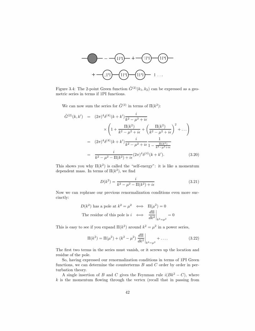
1PI 1PI1PI1PI1PI1PI ++ = + : : :Figure 3.4: The 2-point Green function G(2)(k1, k2) can be expressed as a geo-metric series in terms if 1PI functions.

We can now sum the series for G(2) in terms of Π(k2):

G(2)(k, k′) = (2π)4δ(4)(k + k′)i

k2 − µ2 + iǫ

×(

1 +Π(k2)

k2 − µ2 + iǫ+

(

Π(k2)

k2 − µ2 + iǫ

)2

+ . . .

)

= (2π)4δ(4)(k + k′)i

k2 − µ2 + iǫ

1

1 − Π(k2)k2−µ2+iǫ

=i

k2 − µ2 − Π(k2) + iǫ(2π)4δ(4)(k + k′). (3.20)

This shows you why Π(k2) is called the “self-energy”: it is like a momentumdependent mass. In terms of Π(k2), we find

D(k2) =i

k2 − µ2 − Π(k2) + iǫ(3.21)

Now we can rephrase our previous renormalization conditions even more suc-cinctly:

D(k2) has a pole at k2 = µ2 ⇐⇒ Π(µ2) = 0

The residue of this pole is i ⇐⇒ dΠ

dk2

∣

∣

∣

∣

k2=µ2

= 0

This is easy to see if you expand Π(k2) around k2 = µ2 in a power series,

Π(k2) = Π(µ2) + (k2 − µ2)dΠ

dk2

∣

∣

∣

∣

k2=µ2

+ . . . . (3.22)

The first two terms in the series must vanish, or it screws up the location andresidue of the pole.

So, having expressed our renormalization conditions in terms of 1PI Greenfunctions, we can determine the counterterms B and C order by order in per-turbation theory.

A single insertion of B and C gives the Feynman rule i(Bk2 − C), wherek is the momentum flowing through the vertex (recall that in passing from

42

the Lagrangian to Feynman rules, a derivative acting on an incoming line withmomentum k brings down a factor of −ik). We can write B and C as powerseries expansions,

B =∑

r

Br, C =∑

r

Cr (3.23)

where Br and Cr are of order gr (and B0 = C0 = 0, since there are no inter-actions at O(g0)). Now, suppose we have calculated everything up to O(gn) inperturbation theory, including all counterterms. Then, at O(gn+1), the contri-bution to Π(k2) is given by known stuff (that is, loops we can calculate, includinginsertions of lower order counterterms) plus single insertions of Bn+1 and Cn+1,as shown in Fig. 3.5. Our renormalization conditions (3.22) therefore give us

iBn+1µ2 − iCn+1 = −(known stuff)k2=µ2

iBn+1 = − dknown stuff

dk2

∣

∣

∣

∣

k2=µ2

, (3.24)

determining Bn+1 and Cn+1.1PI += known stu(all Feynman graphs includinginsertions of counterterms upto O(gn)) the only O(gn+1) graphwith only one vertex(n + 1)Figure 3.5: Determining counterterms at O(gn+1).

Similarly, we can calculate the nucleon self-energy, Σ(p2), and impose thecorresponding renormalization conditions

Σ(m2) = 0,dΣ

dp2

∣

∣

∣

∣

p2=m2

= 0. (3.25)

Note that these subtractions do not allow you to ignore corrections to the1PI two point function: Π(k2) has a complicated momentum dependence, andthis is not eliminated by just subtracting the constant and first derivative termsin the vicinity of the pole. Since internal lines are not on shell, this momentumdependence is essential. However, it does solve our problem of loop graphs onexternal legs. Since the LSZ formula comes along with a factor of k2 − µ2 foreach external leg, only the location and residue of the pole are relevant for Smatrix elements.

To see this explicitly, consider the sum of all graphs renormalizing an ex-ternal leg of a diagram, including counterterms, as shown in Fig. 3.6. Thecontribution of this sum of graphs to the amplitude is therefore

limk2→µ2

k2 − µ2

i×D(k2) × (rest of graph)

43

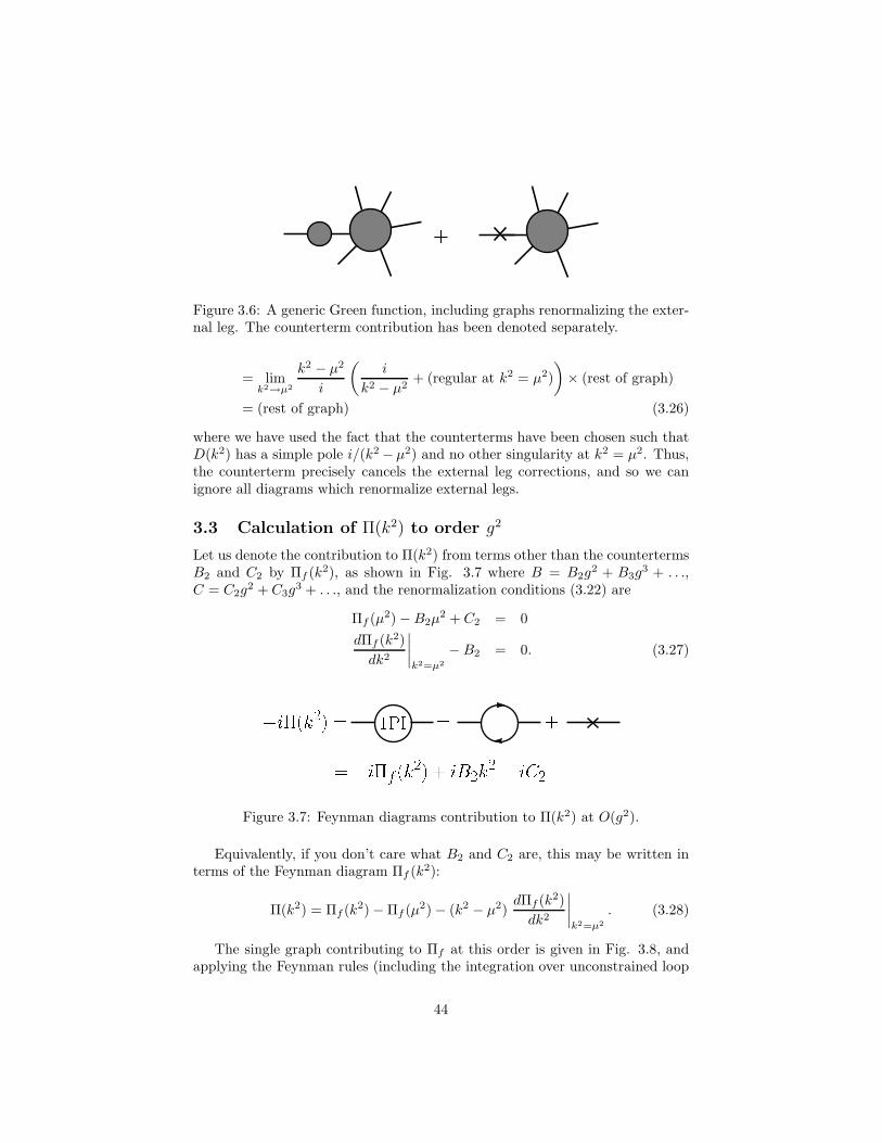
+Figure 3.6: A generic Green function, including graphs renormalizing the exter-nal leg. The counterterm contribution has been denoted separately.

= limk2→µ2

k2 − µ2

i

(

i

k2 − µ2+ (regular at k2 = µ2)

)

× (rest of graph)

= (rest of graph) (3.26)

where we have used the fact that the counterterms have been chosen such thatD(k2) has a simple pole i/(k2 − µ2) and no other singularity at k2 = µ2. Thus,the counterterm precisely cancels the external leg corrections, and so we canignore all diagrams which renormalize external legs.

3.3 Calculation of Π(k2) to order g2

Let us denote the contribution to Π(k2) from terms other than the countertermsB2 and C2 by Πf (k

2), as shown in Fig. 3.7 where B = B2g2 + B3g

3 + . . .,C = C2g

2 + C3g3 + . . ., and the renormalization conditions (3.22) are

Πf (µ2) −B2µ

2 + C2 = 0

dΠf (k2)

dk2

∣

∣

∣

∣

k2=µ2

−B2 = 0. (3.27)

i(k2) = 1PI +== if (k2) + iB2k2 iC2Figure 3.7: Feynman diagrams contribution to Π(k2) at O(g2).

Equivalently, if you don’t care what B2 and C2 are, this may be written interms of the Feynman diagram Πf (k

2):

Π(k2) = Πf (k2) − Πf (µ

2) − (k2 − µ2)dΠf (k

2)

dk2

∣

∣

∣

∣

k2=µ2

. (3.28)

The single graph contributing to Πf at this order is given in Fig. 3.8, andapplying the Feynman rules (including the integration over unconstrained loop

44

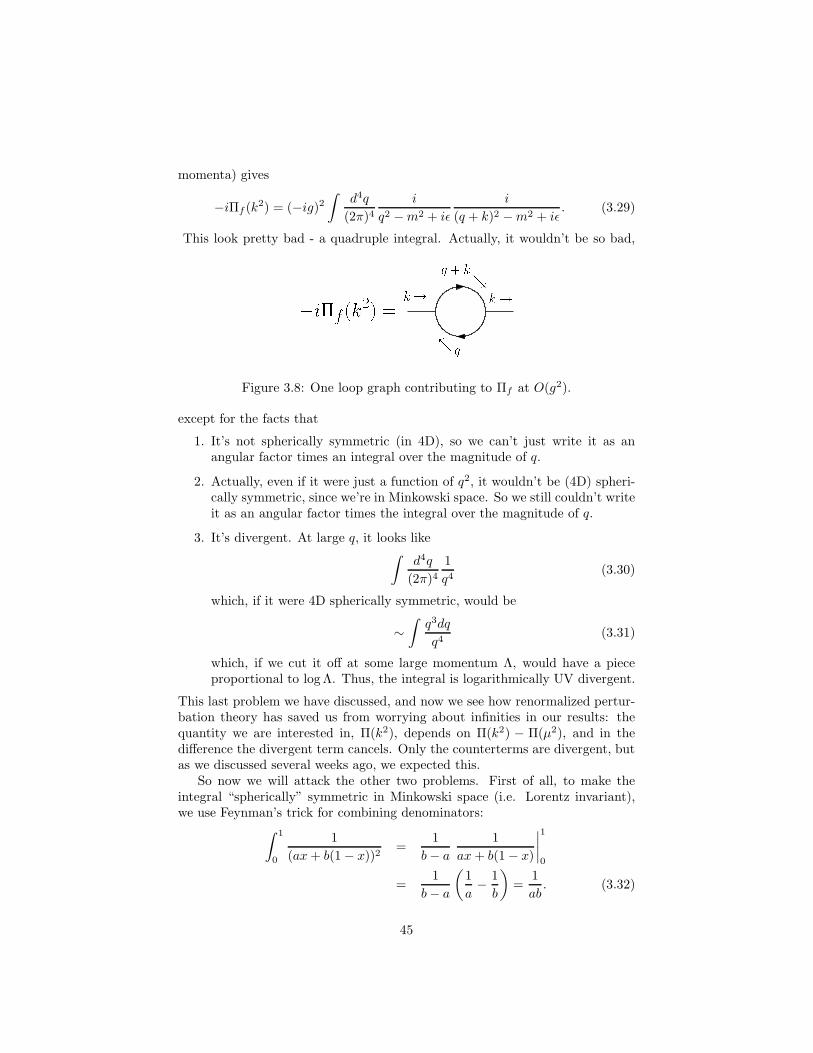
momenta) gives

−iΠf (k2) = (−ig)2

∫

d4q

(2π)4i

q2 −m2 + iǫ

i

(q + k)2 −m2 + iǫ. (3.29)

This look pretty bad - a quadruple integral. Actually, it wouldn’t be so bad,

qq + kk! &- k!if (k2) =

Figure 3.8: One loop graph contributing to Πf at O(g2).

except for the facts that

1. It’s not spherically symmetric (in 4D), so we can’t just write it as anangular factor times an integral over the magnitude of q.

2. Actually, even if it were just a function of q2, it wouldn’t be (4D) spheri-cally symmetric, since we’re in Minkowski space. So we still couldn’t writeit as an angular factor times the integral over the magnitude of q.

3. It’s divergent. At large q, it looks like∫

d4q

(2π)41

q4(3.30)

which, if it were 4D spherically symmetric, would be

∼∫

q3dq

q4(3.31)

which, if we cut it off at some large momentum Λ, would have a pieceproportional to log Λ. Thus, the integral is logarithmically UV divergent.

This last problem we have discussed, and now we see how renormalized pertur-bation theory has saved us from worrying about infinities in our results: thequantity we are interested in, Π(k2), depends on Π(k2) − Π(µ2), and in thedifference the divergent term cancels. Only the counterterms are divergent, butas we discussed several weeks ago, we expected this.

So now we will attack the other two problems. First of all, to make theintegral “spherically” symmetric in Minkowski space (i.e. Lorentz invariant),we use Feynman’s trick for combining denominators:

∫ 1

0

1

(ax+ b(1 − x))2=

1

b− a

1

ax+ b(1 − x)

∣

∣

∣

∣

1

0

=1

b− a

(

1

a− 1

b

)

=1

ab. (3.32)

45

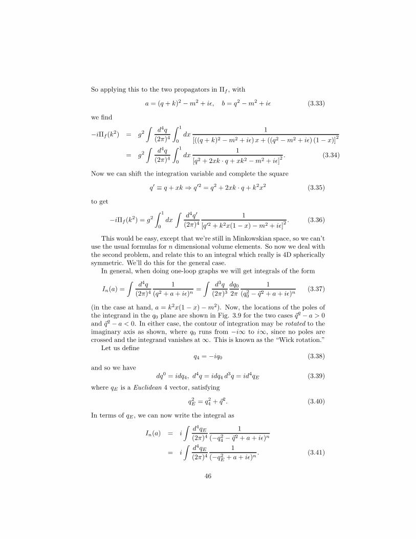
So applying this to the two propagators in Πf , with

a = (q + k)2 −m2 + iǫ, b = q2 −m2 + iǫ (3.33)

we find

−iΠf(k2) = g2

∫

d4q

(2π)4

∫ 1

0

dx1

[((q + k)2 −m2 + iǫ)x+ ((q2 −m2 + iǫ) (1 − x)]2

= g2

∫

d4q

(2π)4

∫ 1

0

dx1

[q2 + 2xk · q + xk2 −m2 + iǫ]2. (3.34)

Now we can shift the integration variable and complete the square

q′ ≡ q + xk ⇒ q′2 = q2 + 2xk · q + k2x2 (3.35)

to get

−iΠf(k2) = g2

∫ 1

0

dx

∫

d4q′

(2π)41

[q′2 + k2x(1 − x) −m2 + iǫ]2. (3.36)

This would be easy, except that we’re still in Minkowskian space, so we can’tuse the usual formulas for n dimensional volume elements. So now we deal withthe second problem, and relate this to an integral which really is 4D sphericallysymmetric. We’ll do this for the general case.

In general, when doing one-loop graphs we will get integrals of the form

In(a) =

∫

d4q

(2π)41

(q2 + a+ iǫ)n=

∫

d3q

(2π)3dq02π

1

(q20 − ~q2 + a+ iǫ)n(3.37)

(in the case at hand, a = k2x(1 − x) −m2). Now, the locations of the poles ofthe integrand in the q0 plane are shown in Fig. 3.9 for the two cases ~q2 − a > 0and ~q2 − a < 0. In either case, the contour of integration may be rotated to theimaginary axis as shown, where q0 runs from −i∞ to i∞, since no poles arecrossed and the integrand vanishes at ∞. This is known as the “Wick rotation.”

Let us defineq4 = −iq0 (3.38)

and so we havedq0 = idq4, d

4q = idq4 d3q = id4qE (3.39)

where qE is a Euclidean 4 vector, satisfying

q2E = q24 + ~q2. (3.40)

In terms of qE , we can now write the integral as

In(a) = i

∫

d4qE(2π)4

1

(−q24 − ~q2 + a+ iǫ)n

= i

∫

d4qE(2π)4

1

(−q2E + a+ iǫ)n. (3.41)

46

(a) (b)q0 q0

Figure 3.9: The Wick rotation: In both the cases ~q2 − a > 0 (a) and ~q2 − a < 0(b), the path of the q0 integration may be rotated as shown in the q0 plane,without crossing any poles.

Now we’re jamming - we have transformed our integral into something which is(four-dimensionally) spherically symmetric. The volume element in 4D space is

∫

d4qE =

∫ ∞

0

q3E dqE

∫

dΩ4 = 2π2

∫ ∞

0

q3E dqE (3.42)

and setting z = q2E , q3E dqE = 12z dz, we get

In(a) =i

16π2

∫ ∞

0

z dz1

(−z + a+ iǫ)n(3.43)

which is straightforward to evaluate.Returning to the case at hand, we need

I2(a) =i

16π2

∫ ∞

0

z dz

(−z + a)2. (3.44)

This is divergent, although the in the combination we are interested the diver-gence cancels. So to make sense of the intermediate steps, let’s regulate theintegral by putting an artifical upper limit Λ2 on the integration, which we willthen take to ∞ at the end:

IΛ2 (a) =

i

16π2

∫ Λ2

0

z dz

(−z + a)2

=i

16π2

(

− ln(−a) +a

a− Λ2+ ln(Λ2 − a) − 1

)

=i

16π2

(

ln Λ2 − 1 − ln(−a))

+ . . . (3.45)

where the dots denote terms which vanish as Λ → ∞. We therefore have

Πf (k2) =

g2

16π2

∫ 1

0

dx ln(−k2x(1 − x) +m2 − iǫ) +g2

16π2

(

ln Λ2 − 1)

(3.46)

47

where the second term will vanish in the convergent combination Πf (k2) −

Πf (µ2). Thus, we find, at long last, the desired result:

Π(k2) = Πf (k2) − Πf (µ

2) − (k2 − µ2)dΠf (k

2)

dk2

∣

∣

∣

∣

k2=µ2

(3.47)

=g2

16π2

∫ 1

0

[

ln−k2x(1 − x) +m2 − iǫ

−µ2x(1 − x) +m2 − iǫ+

(k2 − µ2)x(1 − x)

−µ2x(1 − x) +m2

]

dx

We could actually do the remaining integral without too much trouble (it canbe expressed in terms of arctangents), but it’s not necessary for the discussionwhich follows.

The physical result (3.47) is finite - the only divergence in the calculationhas been cancelled by the divergent counterterm C2.

4 Thus, as expected, thebare mass of the interacting meson field is divergent. One thing we shouldcheck, however, is that the bare mass should still be real; otherwise, the bareLagrangian will not be Hermitian. The only way C2 = −Πf (µ

2) + (convergent)can have a complex piece is if the argument of the logarithm in Eq. (3.46) isless than zero for k2 = µ2; that is, if

µ2x(1 − x) > m2 (3.48)

for x in the range (0, 1). Since the maximum value of x(1 − x) in this intervalis 1/4, this means that C2 will be real as long as

µ2 < 4m2. (3.49)

In other words, as long as the meson is a stable particle, kinematically forbiddento decay to two nucleons, C2 will be real. On the other hand, if it can decay totwo nucleons it looks like its mass counterterm picks up an imaginary piece. Wewill discuss this case shortly, but for the moment we note that this is perhapsnot unexpected, since if the meson can decay we really had no business treatingit as a stable particle anyway. Furthermore, the analytic structure of D(k2) willbe more complicated than we have discussed, since the single particle pole willbe contained within the multiparticle continuum, and we will have to modifyour renormalization conditions accordingly. With these modified conditions, C2

will once again be purely real. As a bonus, we will discover a nice interpretationof the imaginary piece of Π.

Recall that we already determined, on general principles, the analytic struc-ture of

D(k2) =i

k2 − µ2 − Π(k2) + iǫ. (3.50)

Let’s compare this with the one-loop result (3.47). For µ2 < 4m2,∫ 1

0 ln(−k2x(1−x)+m2− iǫ) dx has a branch cut starting at k2 = 4m2, continuing up to k = ∞,

4We would normally expect B2 to be divergent as well. However, this theory is actually aspecial type called a super-renormalizable theory (due to the fact that the coupling constant ghas positive mass dimension) and it has particularly nice UV behaviour. More on this shortly.

48

but it is analytic everywhere else, and the +iǫ prescription says that the valueof the function along the cut is obtained by approaching it from above. Thisagrees with what we found before, from the Lehmann-Kallen spectral represen-tation. It is always reassuring to see that our perturbative result agrees withresults we obtained independent of perturbation theory.

Comments:

1. From Eq. (3.46), we also find

B2 = − g2

16π2

∫

x(1 − x)

m2 − µ2x(1 − x)dx < 0 (for 4m2 > µ2) (3.51)

and since Z = 1 +B, we find Z < 1, as required.

2. Feynman’s trick may be used to combined any number of denominators.Using a similar technique, we find

n∏

r=1

1

ar + iǫ= (n− 1)!

∫ 1

0

dα1 . . . dαn δ(1 −∑

i

αi)1

[∑

r αr(ar + iǫ)]n

= (n− 1)!

∫ 1

0

dα1

∫ 1−α1

0

dα2 . . .

∫ 1−α1...−αn−2

0

dαn−1

1[

∑n−1r=1 αrar +

(

1 −∑n−1r αr

)

an + iǫ]n . (3.52)

3. For n ≥ 3, where the integral is convergent, we have

In(a) =i

16π2(n− 1)(n− 2)an−2. (3.53)

The integral is divergent for n = 1, 2; introducing a cutoff Λ2 we find

I1 =i

16π2a ln(−a) + . . .

I2 = − i

16π2ln(−a) + . . . (3.54)

where the dots denote additional terms which cancel in a convergent sumof such terms (i.e. a sum of such terms such that the total integrandvanishes faster than 1/q4 for high q).

4. Should the fact that the bare mass is divergent be a worry, even philo-sophically? No - the ultraviolet divergence comes from the region of loopintegration where k is very large, and so the distances are correspond-ingly short. Experimentally, we don’t know much about what happens atmomenta greater than about 100 GeV (about 5 × 10( − 17) m), and sowe really can’t expect the integral to be correct above this region. If all

49

particles were actually composite, for example, their interactions would becut off by some form factor at about the scale of their sizes, which wouldmake all the loop integrals finite. However, the beauty of renormalizedperturbation theory is that this is totally irrelevant: any effects of thecutoff Λ which grow with Λ cancel out of physical quantities. If we wereto leave a finite cutoff in the calculation, rather than taking it to ∞, wewould only be left with terms which were suppressed by ptyp/Lambda,where ptyp is the typical momentum in the scattering process of interest.Thus, as long as we are doing physics well below the scale at which thephysics changes, these effects are irrelevant.

5. Finally, note that if we insist that the renormalized mass µ = 0, C2 isstill logarithmically divergent. In other words, a massless meson can onlyarise due to a very precise cancellation between the bare mass and theinteractions - the infinite energy stored in the field surrounding the particleexactly cancels its divergent bare mass to leave a massless particle. Thus,this is an extremely unnatural situation - even if you started with a particlewith vanishing bare mass, the interactions would produce a mass for it.Thus, massless scalar particles are highly unnatural. (This will not be thecase for fermions, as we will see).

3.4 The definition of g

We would like to relate the coupling g in the Lagrangian to some definitionwhich has been approved by a committee of eminent persons. Let us defineΓ(p2, p′2, q2) to be the 1PI three-point function, as shown in Fig. 3.10. Γis defined with an i so that it is always g at leading order in perturbationtheory; however, at higher orders in perturbation theory it will be momentum-dependent. (Note that since Γ is Lorentz invariant, it can only be a functionof scalar products. Since there are only two indepenent momenta, it can onlydepend on p2, p′2 and p · p′, but p · p′ can be traded in for q2.)

1PI = i(p2; p02; q2)p p0q

Figure 3.10: The 1PI three-point function.

A sensible committee definition would be to set Γ(p2, p′2, q2) = g for somefixed point (p2, p′2, q2) in momentum space. Here’s a particularly sensible com-mittee definition:

g = Γ(m2,m2, µ2). (3.55)

50

This point is actually not kinematically accessible (an on-shell nucleon cannotscatter off an on-shell meson and remain on-shell) but nevertheless we will showthat it has a nice experimental significance.

Consider meson-nucleon scattering. We can split all graphs contributing tothis process into 1PI graphs and non-1PI graphs. Now, consider the behaviourof the amplitude as a function of s = (pN + pϕ)2, the invariant mass of thescattering particles. Although s = m2 is kinematically forbidden, we can cer-tainly define our scattering amplitudes there by analytic continuation, and wecan extrapolate our experimental results to this point.

Now, since the 1PI contribution to the amplitude never has a single nucleoncarrying all the incident momentum, it should not have a pole at s = m2, sincethat would indicate the presence of a single-particle resonance. Furthermore, itshouldn’t be hard to convince yourself that all non-1PI contributions to the ratehave the form shown in Fig. 3.11(b), (c) and (d). Of these, only (b) has a poleat s = m2, since at this point the internal nucleon propagator D(s) has pole.Thus, in the vicinity of s = m2, this class of graphs dominates the amplitude,and we have

iA = −iΓ(s,m2, µ2)D(s)(−iΓ(m2, s, µ2))

= −i g2

s−m2+ (regular at s = m2) (3.56)

where the second line follows as a consequence of our renormalization condi-tion, Eq. (3.4). Thus, measuring the scattering amplitude and extrapolating tos = m2 (that is, vanishingly small incident meson momentum) gives a directmeasurement of g with this renormalization condition.

As an aside, if you do this experiment with real nucleons and mesons, youfind g ∼ 13.5. This put the last nail in the coffin in the attempt to describethe nucleon-meson strong interactions via a renormalizable, perturbative fieldtheory such as this model. (Actually, the original experiment was γN → πNinelastic scattering which gives a measurement of eg, since it’s not easy to makepion beams. The general idea was the same, though. )

3.5 Unstable Particles and the Optical Theorem

We now return to the situation where µ > 2m. In this case, Πf (k2) is not real

at k2 = µ2, and so our previous renormalization condition for C yields a non-Hermitian bare Lagrangian. In this section we will modify the renormalizationprescription, and also discover the physical interpretation of the imaginary pieceof Π.

From the spectral representation, it is straightforward to show that

ImΠ(k2) = −π σ(k2)

|D(k2)|2 (3.57)

and so Π picks up an imaginary piece when k is large enough to make multi-particle states - this is a real physical effect and should not be subtracted away

51

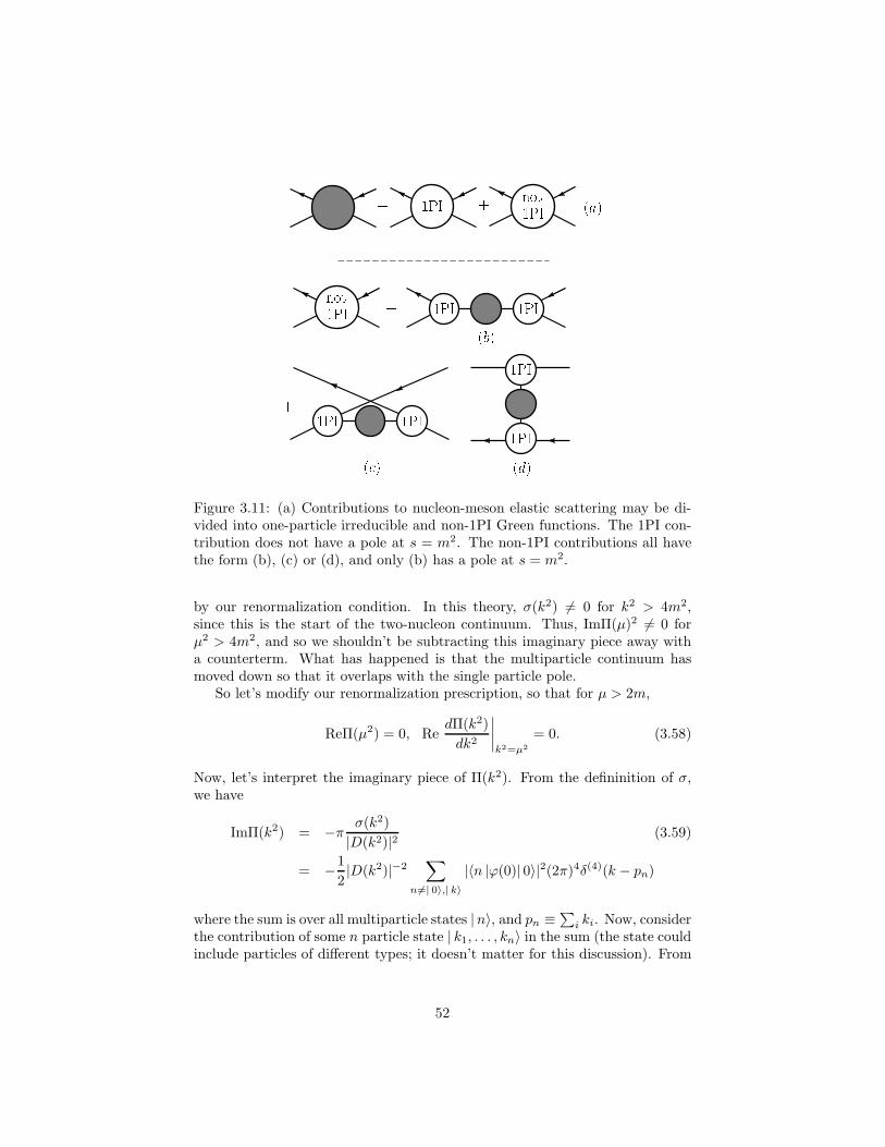
not1PI1PInot1PI 1PI 1PI

1PI1PI1PI1PI

= +

+ +=

(a)(b)

(c) (d)Figure 3.11: (a) Contributions to nucleon-meson elastic scattering may be di-vided into one-particle irreducible and non-1PI Green functions. The 1PI con-tribution does not have a pole at s = m2. The non-1PI contributions all havethe form (b), (c) or (d), and only (b) has a pole at s = m2.

by our renormalization condition. In this theory, σ(k2) 6= 0 for k2 > 4m2,since this is the start of the two-nucleon continuum. Thus, ImΠ(µ)2 6= 0 forµ2 > 4m2, and so we shouldn’t be subtracting this imaginary piece away witha counterterm. What has happened is that the multiparticle continuum hasmoved down so that it overlaps with the single particle pole.

So let’s modify our renormalization prescription, so that for µ > 2m,

ReΠ(µ2) = 0, RedΠ(k2)

dk2

∣

∣

∣

∣

k2=µ2

= 0. (3.58)

Now, let’s interpret the imaginary piece of Π(k2). From the defininition of σ,we have

ImΠ(k2) = −π σ(k2)

|D(k2)|2 (3.59)

= −1

2|D(k2)|−2

∑

n6=| 0〉,|k〉

|〈n |ϕ(0)| 0〉|2(2π)4δ(4)(k − pn)

where the sum is over all multiparticle states |n〉, and pn ≡∑

i ki. Now, considerthe contribution of some n particle state | k1, . . . , kn〉 in the sum (the state couldinclude particles of different types; it doesn’t matter for this discussion). From

52

the LSZ formula and its generalizations, we know that

〈k1, . . . , kn |ϕ(0)| 0〉 =

∫

d4k

(2π)4

n∏

r=1

k2r −m2

r

iG(k1, . . . , kn; k) (3.60)

where the Green function G is illustrated in Fig. 3.12.

kknk1k2k3

Figure 3.12: The Green function which determines 〈k1, . . . , kn |ϕ(0)| 0〉.

Thus, we have

〈k1, . . . , kn |ϕ(0)| 0〉 = [sum of Feynman diagrams] ×D(p2n)

= iAfiD(p2n) (3.61)

where Afi is the usual invariant Feynman amplitude for the process ϕ→ n.Thus, at k2 = µ2, summing over all states |n〉 the factors of the external

meson propagators |D(µ2)| cancel, and we find

ImΠ(k2 = µ2) = −1

2

∑

f

|Afi|2(2π)4δ(4)(k − pn)

= −1

2

∑

n

1

n!

∫

d3p1

(2π)22E1. . .

d3pn(2π)22En

|Afi|2(2π)4δ(4)(k − pn)

= −µΓ (3.62)

where Γ is the decay width of the ϕ, which we calculated last semester. (Thefactors of 1/n! arise from the overcounting of identical particles.)

Now let’s use this result to look at the full meson propagator D(k2) in thevicinity of k2 = µ2. For convenience, let’s look at the region where k2 − µ2 ≤O(g2). Then we have

[−iD(k2)]−1 = k2 − µ2 − Π(µ2) − (k2 − µ2)dΠ

dk2

∣

∣

∣

∣

k2=µ2

+O(g4)

= k2 − µ2 − ReΠ(µ2) − iImΠ(µ2) +O(g4)

= k2 − µ2 + iµΓ +O(g4)

= k2 −(

µ− iΓ

2

)2

+O(g4) (3.63)

53

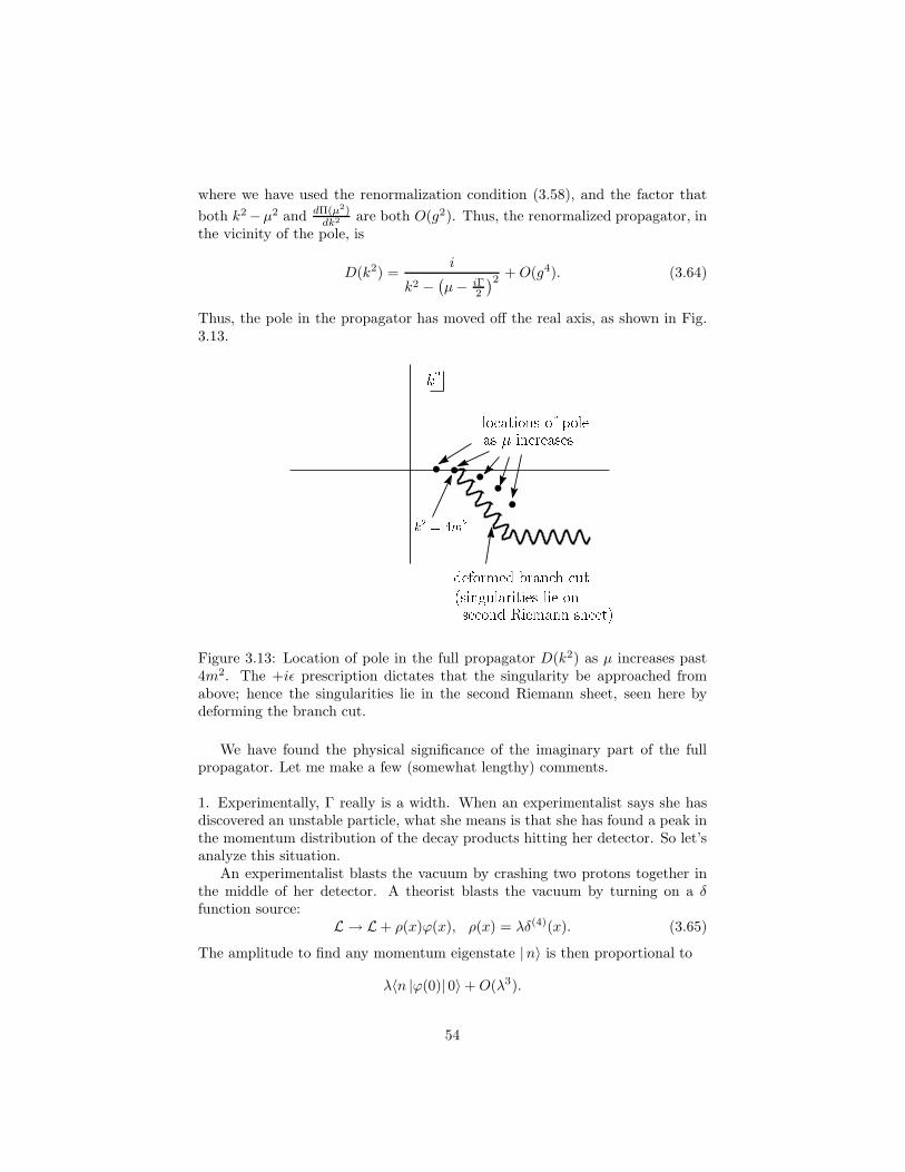
where we have used the renormalization condition (3.58), and the factor that

both k2 −µ2 and dΠ(µ2)dk2 are both O(g2). Thus, the renormalized propagator, in

the vicinity of the pole, is

D(k2) =i

k2 −(

µ− iΓ2

)2 +O(g4). (3.64)

Thus, the pole in the propagator has moved off the real axis, as shown in Fig.3.13. k2

deformed branch cut(singularities lie onsecond Riemann sheet)locations of poleas increases

k2 = 4m2Figure 3.13: Location of pole in the full propagator D(k2) as µ increases past4m2. The +iǫ prescription dictates that the singularity be approached fromabove; hence the singularities lie in the second Riemann sheet, seen here bydeforming the branch cut.

We have found the physical significance of the imaginary part of the fullpropagator. Let me make a few (somewhat lengthy) comments.

1. Experimentally, Γ really is a width. When an experimentalist says she hasdiscovered an unstable particle, what she means is that she has found a peak inthe momentum distribution of the decay products hitting her detector. So let’sanalyze this situation.

An experimentalist blasts the vacuum by crashing two protons together inthe middle of her detector. A theorist blasts the vacuum by turning on a δfunction source:

L → L + ρ(x)ϕ(x), ρ(x) = λδ(4)(x). (3.65)

The amplitude to find any momentum eigenstate |n〉 is then proportional to

λ〈n |ϕ(0)| 0〉 +O(λ3).

54

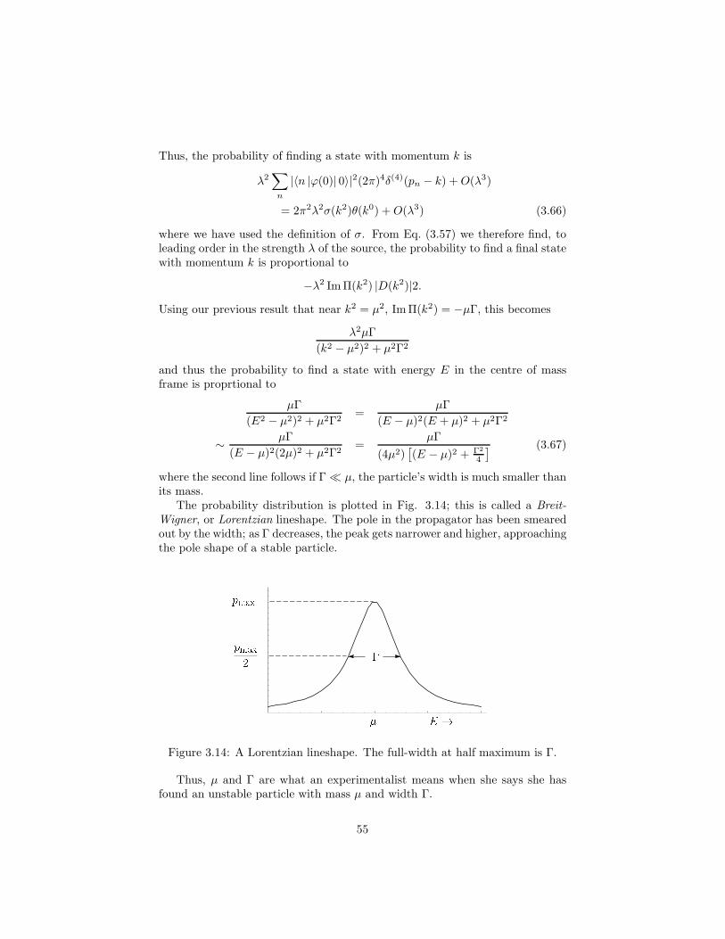
Thus, the probability of finding a state with momentum k is

λ2∑

n

|〈n |ϕ(0)| 0〉|2(2π)4δ(4)(pn − k) +O(λ3)

= 2π2λ2σ(k2)θ(k0) +O(λ3) (3.66)

where we have used the definition of σ. From Eq. (3.57) we therefore find, toleading order in the strength λ of the source, the probability to find a final statewith momentum k is proportional to

−λ2 ImΠ(k2) |D(k2)|2.

Using our previous result that near k2 = µ2, ImΠ(k2) = −µΓ, this becomes

λ2µΓ

(k2 − µ2)2 + µ2Γ2

and thus the probability to find a state with energy E in the centre of massframe is proprtional to

µΓ

(E2 − µ2)2 + µ2Γ2=

µΓ

(E − µ)2(E + µ)2 + µ2Γ2

∼ µΓ

(E − µ)2(2µ)2 + µ2Γ2=

µΓ

(4µ2)[

(E − µ)2 + Γ2

4

] (3.67)

where the second line follows if Γ ≪ µ, the particle’s width is much smaller thanits mass.

The probability distribution is plotted in Fig. 3.14; this is called a Breit-

Wigner, or Lorentzian lineshape. The pole in the propagator has been smearedout by the width; as Γ decreases, the peak gets narrower and higher, approachingthe pole shape of a stable particle.

19 20 21 22

1

2

3

4

5

pmaxpmax2

E !Figure 3.14: A Lorentzian lineshape. The full-width at half maximum is Γ.

Thus, µ and Γ are what an experimentalist means when she says she hasfound an unstable particle with mass µ and width Γ.

55

2. The previous comment actually justifies our previous expression for Γ, whichwe obtained in the theory with a turning on and off function. The problem is,you can’t use the LSZ formula in the usual way to calculate the width, sinceyou can’t make an “in” state of an unstable particle - it decays away in the timefrom t = −∞ to t = 0. So instead, we get the expression for the partial decaywidth dΓ to some final state |n〉 by taking the matrix element

out〈n |ϕ(0)| 0〉

which we can evaluate via the extended form of the LSZ formula discussed inthe last chapter. That is, we blast the vacuum at t = 0, and look at the outstates this produces in the region of the single-particle pole.

3. This is an example of a more general result, known as the Optical Theorem.This actually goes back to scattering theory in quantum mechanics. There itwas based on a simple idea: there is an incoming wave incident on a target, andan outgoing wave. The outgoing wave is the superpositioni of the incoming wavethat passes right through the target and the scattered wave. By conservationof probability, if the wave is scattered there must be a decrease in the intensityof the beam in the forward direction.

The total probability to scatter in any direction but directly forward is pro-portional to the cross section σ. This therefore is equal to the decrease inthe probability of going exactly forward, which is the interference between theunscattered and scattered waves.

The field theory version of the optical theorem is trivial to derive. By con-servation of probability,

S†S = 1

and thus we have

(S − 1)(S − 1)† = SS† − S − S† + 1 = −(S − 1) − (S − 1)†. (3.68)

Now consider the case of forward scattering. Taking the matrix element of thisresult between the in and out states | f〉 and | i〉, and inserting a complete setof states |n〉 we have

∑

n

〈f |(S − 1)|n〉〈n |(S − 1)†| i〉 − 〈f |(S − 1)| i〉 − 〈f |(S − 1)†| i〉. (3.69)

Working on the LHS, we find5

LHS =∑

n

∫

d3k1 . . . d3kn

(2π)32E1 . . . (2π)32EnAfmA∗

im

×(2π)4δ(4)(pf − pm)(2π)4δ(4)(pi − pm). (3.70)

5In the case in which some of the nm particles are identical, we will have additional factorsof 1/nm! in these formulas.

56

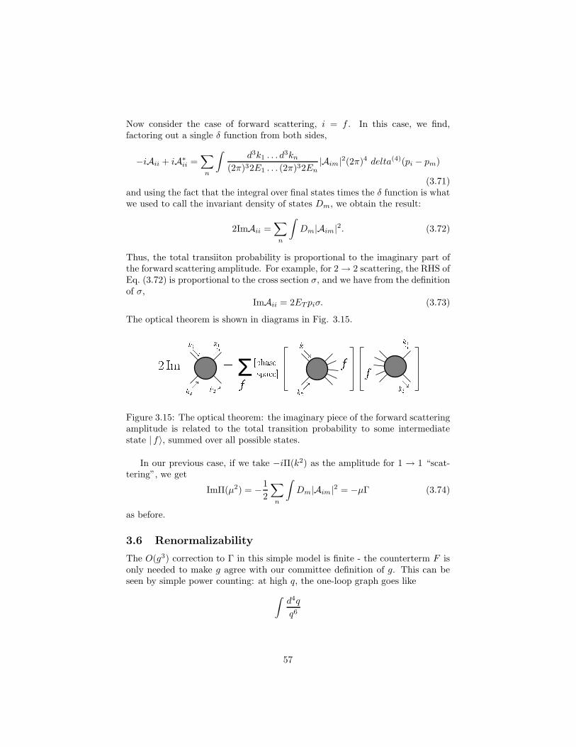
Now consider the case of forward scattering, i = f . In this case, we find,factoring out a single δ function from both sides,

−iAii + iA∗ii =

∑

n

∫

d3k1 . . . d3kn

(2π)32E1 . . . (2π)32En|Aim|2(2π)4 delta(4)(pi − pm)

(3.71)and using the fact that the integral over final states times the δ function is whatwe used to call the invariant density of states Dm, we obtain the result:

2ImAii =∑

n

∫

Dm|Aim|2. (3.72)

Thus, the total transiiton probability is proportional to the imaginary part ofthe forward scattering amplitude. For example, for 2 → 2 scattering, the RHS ofEq. (3.72) is proportional to the cross section σ, and we have from the definitionof σ,

ImAii = 2ET piσ. (3.73)

The optical theorem is shown in diagrams in Fig. 3.15.

2 Im k1k2 k2k1%& %& = Σ k2k1%&fk1k2%& ff [phasespace]

Figure 3.15: The optical theorem: the imaginary piece of the forward scatteringamplitude is related to the total transition probability to some intermediatestate | f〉, summed over all possible states.

In our previous case, if we take −iΠ(k2) as the amplitude for 1 → 1 “scat-tering”, we get

ImΠ(µ2) = −1

2

∑

n

∫

Dm|Aim|2 = −µΓ (3.74)

as before.

3.6 Renormalizability

The O(g3) correction to Γ in this simple model is finite - the counterterm F isonly needed to make g agree with our committee definition of g. This can beseen by simple power counting: at high q, the one-loop graph goes like

∫

d4q

q6

57

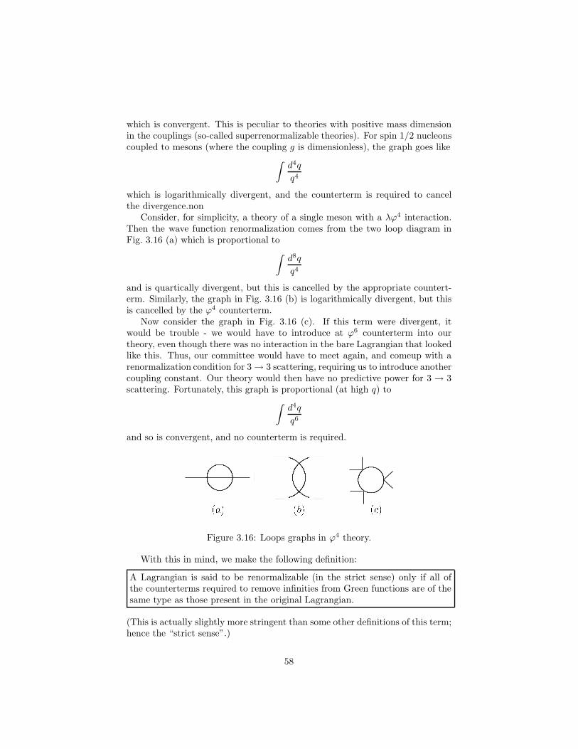
which is convergent. This is peculiar to theories with positive mass dimensionin the couplings (so-called superrenormalizable theories). For spin 1/2 nucleonscoupled to mesons (where the coupling g is dimensionless), the graph goes like

∫

d4q

q4

which is logarithmically divergent, and the counterterm is required to cancelthe divergence.non

Consider, for simplicity, a theory of a single meson with a λϕ4 interaction.Then the wave function renormalization comes from the two loop diagram inFig. 3.16 (a) which is proportional to

∫

d8q

q4

and is quartically divergent, but this is cancelled by the appropriate countert-erm. Similarly, the graph in Fig. 3.16 (b) is logarithmically divergent, but thisis cancelled by the ϕ4 counterterm.

Now consider the graph in Fig. 3.16 (c). If this term were divergent, itwould be trouble - we would have to introduce at ϕ6 counterterm into ourtheory, even though there was no interaction in the bare Lagrangian that lookedlike this. Thus, our committee would have to meet again, and comeup with arenormalization condition for 3 → 3 scattering, requiring us to introduce anothercoupling constant. Our theory would then have no predictive power for 3 → 3scattering. Fortunately, this graph is proportional (at high q) to

∫

d4q

q6

and so is convergent, and no counterterm is required.

(a) (b) (c)Figure 3.16: Loops graphs in ϕ4 theory.

With this in mind, we make the following definition:

A Lagrangian is said to be renormalizable (in the strict sense) only if all ofthe counterterms required to remove infinities from Green functions are of thesame type as those present in the original Lagrangian.

(This is actually slightly more stringent than some other definitions of this term;hence the “strict sense”.)

58

For example, suppose we had a ϕ5 interaction. Then the graph in Fig. 3.17(a) is logarithmically divergent, so we would need a ϕ6 counterterm. Thus,ϕ5 theory is not renormalizable. Of course, we could add a ϕ5 term to the La-grangian, but then you’d get graphs like those in Fig. 3.17 (b) and (c), requiringϕ7 and ϕ8 terms, and so on. The problem with this, as we have already men-tioned, is that the theory would no longer have predictive power. Our committeewould have to come up with an infinite number of renormalization conditionsfor 2 → 3, 2 → 4, . . . , 2 → n scattering, and so our theory would have an infinitenumber of adjustable parameters.6

(a) (b) (c)Figure 3.17: Divergent loops graphs (a) in ϕ5 theory, (b, c) with a ϕ6 countert-erm added.

Thus, theories with polynomial interactions of scalars with more than fourfields are nonrenormalizable. Although we haven’t proved it, it seems plausiblethat scalar theories with poynomial interactions with four or fewer fields arerenormalizable. In the next section we will study this problem in more detail,and determine the conditions for a general field theory to be renormalizable.

6Actually, this statement is a bit misleading. As we may discuss later in the course, non-renormalizable theories can be very useful. Even though they cannot make exact predictionswithout tuning an arbitrary number of parameters, the effects of operators of higher andhigher dimension are suppressed by powers of the momentum relevant to a given process oversome large momentum scale where new physics comes into play. It turns out that nonrenor-malizable Lagrangians are very useful for calculating in theories with widely separated massscales.

59

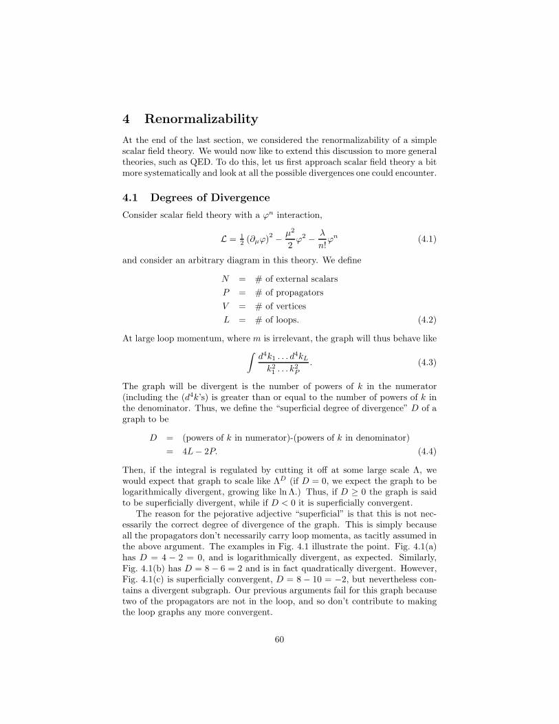
4 Renormalizability

At the end of the last section, we considered the renormalizability of a simplescalar field theory. We would now like to extend this discussion to more generaltheories, such as QED. To do this, let us first approach scalar field theory a bitmore systematically and look at all the possible divergences one could encounter.

4.1 Degrees of Divergence

Consider scalar field theory with a ϕn interaction,

L = 12 (∂µϕ)

2 − µ2

2ϕ2 − λ

n!ϕn (4.1)

and consider an arbitrary diagram in this theory. We define

N = # of external scalars

P = # of propagators

V = # of vertices

L = # of loops. (4.2)

At large loop momentum, where m is irrelevant, the graph will thus behave like

∫

d4k1 . . . d4kL

k21 . . . k

2P

. (4.3)

The graph will be divergent is the number of powers of k in the numerator(including the (d4k’s) is greater than or equal to the number of powers of k inthe denominator. Thus, we define the “superficial degree of divergence” D of agraph to be

D = (powers of k in numerator)-(powers of k in denominator)

= 4L− 2P. (4.4)

Then, if the integral is regulated by cutting it off at some large scale Λ, wewould expect that graph to scale like ΛD (if D = 0, we expect the graph to belogarithmically divergent, growing like ln Λ.) Thus, if D ≥ 0 the graph is saidto be superficially divergent, while if D < 0 it is superficially convergent.

The reason for the pejorative adjective “superficial” is that this is not nec-essarily the correct degree of divergence of the graph. This is simply becauseall the propagators don’t necessarily carry loop momenta, as tacitly assumed inthe above argument. The examples in Fig. 4.1 illustrate the point. Fig. 4.1(a)has D = 4 − 2 = 0, and is logarithmically divergent, as expected. Similarly,Fig. 4.1(b) has D = 8 − 6 = 2 and is in fact quadratically divergent. However,Fig. 4.1(c) is superficially convergent, D = 8 − 10 = −2, but nevertheless con-tains a divergent subgraph. Our previous arguments fail for this graph becausetwo of the propagators are not in the loop, and so don’t contribute to makingthe loop graphs any more convergent.

60

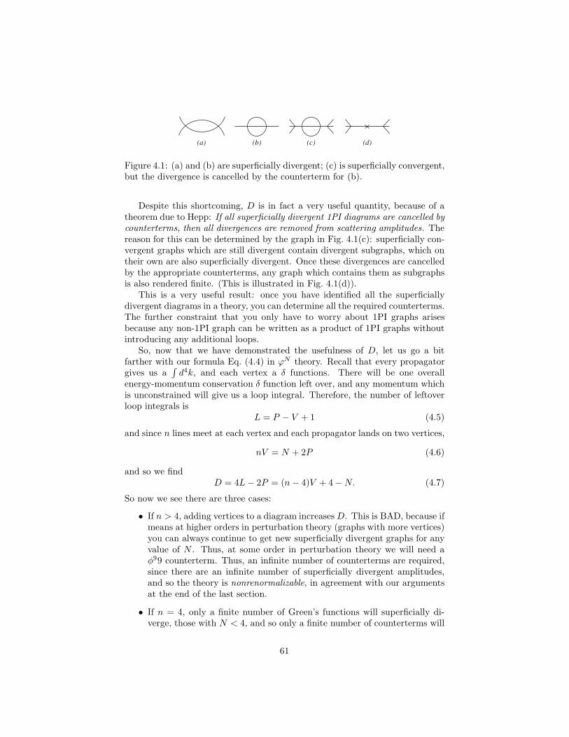
(a) (b) (c) (d)

Figure 4.1: (a) and (b) are superficially divergent; (c) is superficially convergent,but the divergence is cancelled by the counterterm for (b).

Despite this shortcoming, D is in fact a very useful quantity, because of atheorem due to Hepp: If all superficially divergent 1PI diagrams are cancelled by

counterterms, then all divergences are removed from scattering amplitudes. Thereason for this can be determined by the graph in Fig. 4.1(c): superficially con-vergent graphs which are still divergent contain divergent subgraphs, which ontheir own are also superficially divergent. Once these divergences are cancelledby the appropriate counterterms, any graph which contains them as subgraphsis also rendered finite. (This is illustrated in Fig. 4.1(d)).

This is a very useful result: once you have identified all the superficiallydivergent diagrams in a theory, you can determine all the required counterterms.The further constraint that you only have to worry about 1PI graphs arisesbecause any non-1PI graph can be written as a product of 1PI graphs withoutintroducing any additional loops.

So, now that we have demonstrated the usefulness of D, let us go a bitfarther with our formula Eq. (4.4) in ϕN theory. Recall that every propagatorgives us a

∫

d4k, and each vertex a δ functions. There will be one overallenergy-momentum conservation δ function left over, and any momentum whichis unconstrained will give us a loop integral. Therefore, the number of leftoverloop integrals is

L = P − V + 1 (4.5)

and since n lines meet at each vertex and each propagator lands on two vertices,

nV = N + 2P (4.6)

and so we findD = 4L− 2P = (n− 4)V + 4 −N. (4.7)

So now we see there are three cases:

• If n > 4, adding vertices to a diagram increasesD. This is BAD, because ifmeans at higher orders in perturbation theory (graphs with more vertices)you can always continue to get new superficially divergent graphs for anyvalue of N . Thus, at some order in perturbation theory we will need aφ99 counterterm. Thus, an infinite number of counterterms are required,since there are an infinite number of superficially divergent amplitudes,and so the theory is nonrenormalizable, in agreement with our argumentsat the end of the last section.

• If n = 4, only a finite number of Green’s functions will superficially di-verge, those with N < 4, and so only a finite number of counterterms will

61

be required to make all amplitudes finite. This class of theory is calledrenormalizable. Note that there will be divergent graphs at all orders inperturbation theory, but only for Green functions with less than or equalto N external legs.

• If n < 4, not only is the theory renormalizable, but each time you add avertex you make any given graph more convergent. In this case, not only isthe number of superficially divergent Green functions finite, but the num-ber of superficially divergent graphs is finite. Divergences are restrictedto low orders in perturbation theory (so that V isn’t too big), in contrastwith renormalizable theories, where divergences occur at all orders in per-turbation theory. This class of theory is called super-renormalizable; theψ∗ψϕ theory we have been playing with is in this class.

Now that we have formulated our criteria for renormalizability in a moregeneral way, we can determine all necessary counterterms just be writing downall superficially divergent amplitudes. For example, in ϕ4 theory, we have D =4 −N , and so the only superficially divergent amplitudes have N ≤ 4:

1. N = 0: This is a zero-point Green function, just correponding to thevacuum energy, and is cancelled by the appropriate constant energy shift.

2. N = 1, 3: No such counterterms can exist, because L is invariant underthe symmetry ϕ→ −ϕ, and such terms break this symmetry.

3. N = 2: The self-energy graph has D = 2. We can Taylor expand thisamplitude in powers of p, the external momentum, to a series of the forma0 +a1p

2+a2p4 + . . . . Now, each term in the expansion will have a smaller

D than the previous one, since each time we differentiate the amplitudewith respect to p it reduces the degree of divergence by 1 (adding onepower of momentum to the denominator of the loop integral). Thus, a0 isquadratically divergent (D = 2), but a0 is only logarithmically divergent(D = 0) while all other ai’s are convergent. Thus, this Green functionhas two independent divergences, requiring two counterterms of the formAp2 +B. These are just mass and wavefunction renormalization.

4. N = 4: The four-point function has D = 0, so diverges like ln Λ. Ittherefore requires a single counterterm.

That’s it! As expected, there are no superficially divergent amplitudes withmore than 4 external legs.

We can also compare this result with the superrenormalizable ψ∗ψϕ theory.In this case, we have D = 4−N−V . For the two-point function, D = 2−V andso the only graph with D > 0 is the one-loop 1PI graph we calculated in the lastchapter! Since D = 0, it is log divergent, so expanding the amplitude as a0 +a1p

2+. . ., only a0 is divergent, requiring a mass counterterm. As we found in thelast chapter, the wavefunction renormalization is finite. Furthermore, graphs athigher orders in perturbation theory are all superficially convergent, since they

62

will have V > 2. Similarly, the one-loop renormalization of g already has D =4 − 3 − 3 = −2, and so there is no divergent coupling constant renormalizationin this theory, as we found.

A few comments:

1. The renormalizability of a theory depends on the number of dimensionsyou are working in. More generally, for ϕn theory in d dimensions, similarmanipulations yield

D = d+

[

n

(

d− 2

2

)

− d

]

V −(

d− 2

2

)

N. (4.8)

Ths, ϕ4 theory is renormalizable in four dimensions, while in three dimen-sions it is superrenormalizable, and ϕ6 theory is renormalizable. In twodimensions, ϕn theory is renormalizable for any n. We can also summarizethis in terms of dimensional analysis. In d dimensions, [L] = d (so that theaction is dimensionless), and since [m2ϕ2] = d, we have [ϕ] = (d − 2)/2.Thus, [λϕn] = d, and the units of the coupling constant λ in ϕn theory ind dimensions are [λ] = d − n[ϕ] = d − n(d − 2)/2. Comparing this withEq. (4.8), we find that

(a) [λ] > 0 (the coupling has positive mass dimension → the theory issuperrenormalizable

(b) [λ] = 0 (the coupling is dimensionless) → the theory is renormalizable

(c) [λ] < 0 (the coupling has negative mass dimension) → the theory isnonrenormalizable.

As we shall see, this requirement is generally true, even in theories withfermions and (with additional restrictions) gauge bosons. Thus, the classof renormalizable theories in four dimensions is very small - only termswith dimension ≤ 4 are allowed.

2. It is straightforward to add spin 1/2 fermions to this discussion, as well asderivative interactions such as ϕ2∂µϕ∂

µϕ. Fermions contribute differentlyto D than bosons since their propagators don’t fall off as fast for large k- like 1/k/ instead of 1/k2. Thus, in this case we have

D = 4L− 2PB − PF (4.9)

where PB is the number of scalar boson propagators and PF is the numberof spin 1/2 fermion propagators. Now suppose that the Lagrangian is ofthe form

L = L0 +∑

i

λiLi (4.10)

where the i’th interaction vertex contains

bi scalar bosons

fi spin 1/2 fermiosn

di derivatives

63

and has coupling constant λi. Then, going through the same rigamaroleas before, we find that a graph with ni vertices of type i has (in fourdimensions)

D = 4 −NB − 3/2NF +∑

i

niδi (4.11)

whereδi ≡ di + bi + 3/2fi − 4 (4.12)

is the “index of divergence” of the interaction Li. (Note that becauseof their slower UV falloff, fermions give a larger contribution to D thanscalars). THus, if any interaction has positive index of divergence, thetheory is nonrenormalizable, since by adding vertices a positive D may beobtained for any value of NB and NF . But again, even in this case, infour dimensions we have [ϕ] = 1, [ψ] = 3/2, and so δi = [Li] − 4 = −[λi].Thus, as before, we find that as long as all λi’s are ≥ 0 (have positive orzero mass dimension) the theory is renormalizable.

3. Generally, all renormalizable interactions are required to absorb diver-gences in superficially divergent subgraphs. For example, consider a pseudoscalar-fermion-antifermion coupling

LI = −igψγ5ψϕ. (4.13)

The coupling g has 0 mass dimension. However, this theory is not, strictlyspeaking, renormalizable. The box graph in Fig. 4.2 is logarithmicallydivergent (D = 0), and so it will need a ϕ4 counterterm, which wasn’toriginally present in Li. However, the interaction

Figure 4.2: Logarithmically divergent “box graph”.

LI = −igψγ5ψϕ+λ

4ϕ4 (4.14)

is, strictly speaking, renormalizable. This is also in accord with our earlierassertion that massless scalars are unnatural - even if the renormalizedmass µ is set to zero, a mass counterterm is nevertheless required.

4. There is one exception to the above rule: a theory which is invariantunder some internal symmetry will not need all terms with d ≤ 4 tobe renormalizable, but only those consistent with the symmetry. In theabove example, for instance, the Lagrangian is invariant under parity,

64

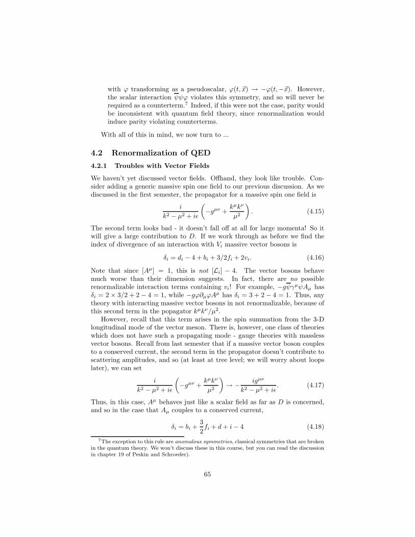
with ϕ transforming as a pseudoscalar, ϕ(t, ~x) → −ϕ(t,−~x). However,the scalar interaction ψψϕ violates this symmetry, and so will never berequired as a counterterm.7 Indeed, if this were not the case, parity wouldbe inconsistent with quantum field theory, since renormalization wouldinduce parity violating counterterms.

With all of this in mind, we now turn to ...

4.2 Renormalization of QED

4.2.1 Troubles with Vector Fields

We haven’t yet discussed vector fields. Offhand, they look like trouble. Con-sider adding a generic massive spin one field to our previous discussion. As wediscussed in the first semester, the propagator for a massive spin one field is

i

k2 − µ2 + iǫ

(

−gµν +kµkν

µ2

)

. (4.15)

The second term looks bad - it doesn’t fall off at all for large momenta! So itwill give a large contribution to D. If we work through as before we find theindex of divergence of an interaction with Vi massive vector bosons is

δi = di − 4 + bi + 3/2fi + 2vi. (4.16)

Note that since [Aµ] = 1, this is not [Li] − 4. The vector bosons behavemuch worse than their dimension suggests. In fact, there are no possiblerenormalizable interaction terms containing vi! For example, −gψγµψAµ hasδi = 2 × 3/2 + 2 − 4 = 1, while −gϕ∂µϕAµ has δi = 3 + 2 − 4 = 1. Thus, anytheory with interacting massive vector bosons in not renormalizable, because ofthis second term in the popagator kµkν/µ2.

However, recall that this term arises in the spin summation from the 3-Dlongitudinal mode of the vector meson. There is, however, one class of theorieswhich does not have such a propagating mode - gauge theories with masslessvector bosons. Recall from last semester that if a massive vector boson couplesto a conserved current, the second term in the propagator doesn’t contribute toscattering amplitudes, and so (at least at tree level; we will worry about loopslater), we can set

i

k2 − µ2 + iǫ

(

−gµν +kµkν

µ2

)

→ − igµν

k2 − µ2 + iǫ. (4.17)

Thus, in this case, Aµ behaves just like a scalar field as far as D is concerned,and so in the case that Aµ couples to a conserved current,

δi = bi +3

2fi + d+ i− 4 (4.18)

7The exception to this rule are anomalous symmetries, classical symmetries that are brokenin the quantum theory. We won’t discuss these in this course, but you can read the discussionin chapter 19 of Peskin and Schroeder).

65

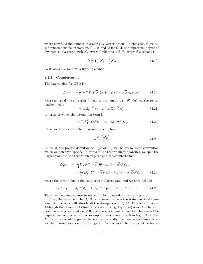
where now bi is the number of scalar plus vector bosons. In this case, ψγµψAµis a renormalizable interaction, δi = 0, and so for QED the superficial degree ofdivergence of a graph with Nγ external photons and Ne external electrons is

D = 4 −Nγ −3

2Ne. (4.19)

So it looks like we have a fighting chance.

4.2.2 Counterterms

The Lagrangian for QED is

LQED = −1

4(Fµν0 )

2+ ψ0 (i∂/+m0)ψ0 − e0ψ0γµψ0A

µ0 (4.20)

where as usual the subscript 0 denotes bare quantites. We defined the renor-malized fields

ψ ≡ Z−1/22 ψ0, Aµ ≡ Z

−1/23 Aµ0 (4.21)

in terms of which the interaction term is

−e0Z2Z1/23 ψγµψAµ ≡ −eZ1ψγ

µψAµ (4.22)

where we have defined the renormalized coupling

e =e0Z2Z

1/23

Z1. (4.23)

As usual, the precise definition of e (or of Z1) will be set by some conventionwhich we don’t yet specify. In terms of the renormalized quantites, we split theLagrangian into the renormalized piece and the counterterms:

LQED =1

4FµνF

µν + ψ (i∂/−m)ψ − eψγµψAµ

−1

4δ3FµνF

µν + ψ (iδ2∂/− δm)ψ − eδ1ψγµψAµ (4.24)

where the second line is the counterterm Lagrangian, and we have defined

δ3 ≡ Z3 − 1, δ2 ≡ Z2 − 1, δm ≡ Z2m0 −m, δ1 ≡ Z1 − 1. (4.25)

Thus, we have four counterterms, with Feynman rules given in Fig. 4.3.Now, the statement that QED is renormalizable is the statement that these

four counterterms will absorb all the divergences of QED. This isn’t obvious!Although the theory looks fine by power counting, Eq. (4.24) doesn’t include allpossible interactions with δi ≤ 0, and there is no guarantee that these won’t berequired as counterterms. For example, the one loop graph in Fig. 4.4 (a) hasD = 2, so we would expect to have a quadratically divergent mass countertermfor the photon, as shown in the figure. Furthermore, the four point vertex in

66

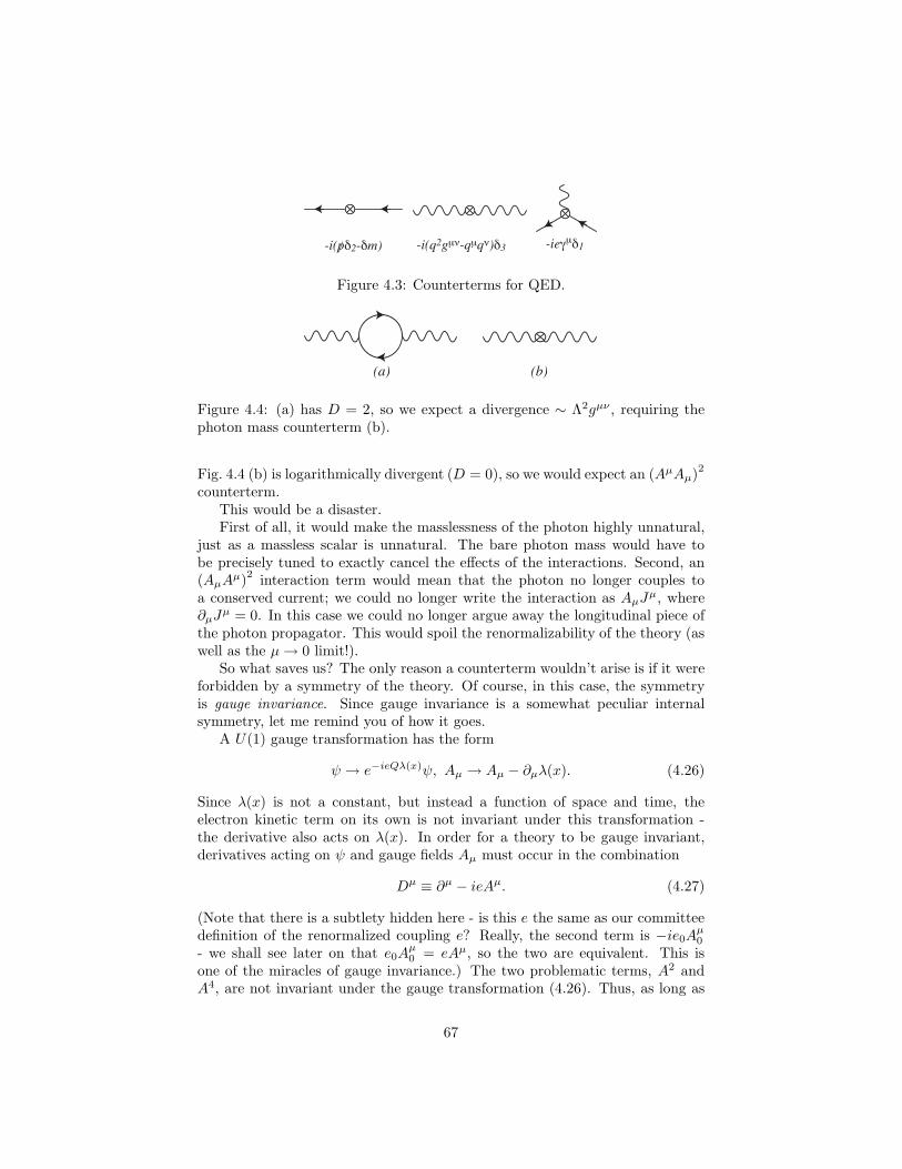
-i(q2gµν-qµqν)δ3 -ieγµδ1-i(pδ2-δm)/

Figure 4.3: Counterterms for QED.

(a) (b)

Figure 4.4: (a) has D = 2, so we expect a divergence ∼ Λ2gµν , requiring thephoton mass counterterm (b).

Fig. 4.4 (b) is logarithmically divergent (D = 0), so we would expect an (AµAµ)2

counterterm.This would be a disaster.First of all, it would make the masslessness of the photon highly unnatural,

just as a massless scalar is unnatural. The bare photon mass would have tobe precisely tuned to exactly cancel the effects of the interactions. Second, an(AµA

µ)2

interaction term would mean that the photon no longer couples toa conserved current; we could no longer write the interaction as AµJ

µ, where∂µJ

µ = 0. In this case we could no longer argue away the longitudinal piece ofthe photon propagator. This would spoil the renormalizability of the theory (aswell as the µ→ 0 limit!).

So what saves us? The only reason a counterterm wouldn’t arise is if it wereforbidden by a symmetry of the theory. Of course, in this case, the symmetryis gauge invariance. Since gauge invariance is a somewhat peculiar internalsymmetry, let me remind you of how it goes.

A U(1) gauge transformation has the form

ψ → e−ieQλ(x)ψ, Aµ → Aµ − ∂µλ(x). (4.26)

Since λ(x) is not a constant, but instead a function of space and time, theelectron kinetic term on its own is not invariant under this transformation -the derivative also acts on λ(x). In order for a theory to be gauge invariant,derivatives acting on ψ and gauge fields Aµ must occur in the combination

Dµ ≡ ∂µ − ieAµ. (4.27)

(Note that there is a subtlety hidden here - is this e the same as our committeedefinition of the renormalized coupling e? Really, the second term is −ie0Aµ0- we shall see later on that e0A

µ0 = eAµ, so the two are equivalent. This is

one of the miracles of gauge invariance.) The two problematic terms, A2 andA4, are not invariant under the gauge transformation (4.26). Thus, as long as

67

gauge symmetry is preserved by renormalization, they shouldn’t arise. However,since gauge symmetries are not as straightforward as global symmetries, thisagain isn’t obvious. Let’s see how it works. First, however, recall one of theconsequences of coupling a photon to a conserved current that we discoveredlast semester. An amplitude with an external photon with polarization ǫµ willhave the form ǫµMµ, where Mµ is the rest of the diagram. We found that aslong as the current is conserved,

kµMµ = 0. (4.28)

This just follows from ∂µJµ = 0, and is known as the Ward Identity, and it tells

us that the helicity zero mode of the photon decouples, since the helicity zeromode has ǫµ ∝ kµ.

We will prove the Ward Identity (and its generalization) soon, but for themoment let us assume it remains true beyond tree level.

Now let us look at all the 1PI graphs with D > 0 in QED. There are six,as illustrated in Fig. 4.5, where the starred Green functions denote possibletrouble, since they have no gauge invariant counterterms.

(a) (b) (c)

(d) (e) (f)

Figure 4.5: Superficially divergent Green’s function in QED.

We will dispatch with the easy ones first. (a) is just the vacuum energycounterterm, which is trivial. (c) corresponds to electron mass and wavefunctionrenormalization. Expanding in powers of p/,

(c) ∼ A0 +A1p/+A2p2 + . . . (4.29)

the usual arguments would lead us to expect that A0 is linearly divergent, ∼ Λ,A1 ∼ ln Λ, and all the other A’s are finite. Thus, there are two infinities, A0

and A1, and two counterterms, δ2 and δm, so all is well. Actually, there is asubtlety here. A theory with massless fermions has an extra symmetry, chiral

symmetry, since the left- and right-handed helicity modes of a massless fermiondecouple. Thus, we can perform independent U(1) transformations on the twohelicities,

ψL → eiαψL, ψR → eiβψR. (4.30)

68

A mass counterterm δmψψ = δm(

ψLψR + ψRψL)

breaks this symmetry downto the diagonal U(1) of fermion number, and so is forbidden. (Thus, in contrastto scalars, massless fermions are quite natural, since they are protected fromgetting a mass by a symmetry). As far as our counterterms go, it means thatA0 vanishes when m = 0, so by dimensional analysis it must be proportional tom lnΛ, and not Λ, so is only logarithmically divergent.

Diagram (e) is straightforward - it has D = 0 and so has a single logarithmicdivergence proportional to −ieγµ ln Λ, which is cancelled by δ1.

Diagram (d) would required a counterterm proportional to A3. However,this amplitude is actually zero - it is forbidden by charge conjugation symmetry.(This result is known as “Furry’s Theorem.”) Recall that the charge conjugationoperator C changes particles to antiparticles. You can easily show that thisimplies that the electromagnetic current operator must flip sign under C:

CJµC† = −Jµ (4.31)

where Jµ = ψγµψ is the electromagnetic current. Since the three-point functionis related to the Fourier transform of

〈0 |T (Jµ(x1)Jν(x2)J

α(x3)) | 0〉 (4.32)

we can act with the C operator to show that

〈0 |Jµ(x1)Jν(x2)J

α(x3)| 0〉 = 〈0 |CC†Jµ(x1)CC†Jν(x2)CC

†Jα(x3)CC†| 0〉

= −〈0 |Jµ(x1)Jν(x2)J

α(x3)| 0〉 (4.33)

since CC† = 1 and the vacuum is invariant under charge conjugation, C| 0〉 =| 0〉. Thus, the matrix element of an odd number of currents vanishes, so thephoton three-point function in QED is identically zero.

This leaves us with diagram (b). This one looks like trouble. Defining thephoton self-energy Πµν in analogy with the scalar self energy, we can split Πµν

up into two Lorentz structures,

Πµν(q) = agµν + b(

gµνq2 − qµqν)

. (4.34)

A divergence in b is fine - this is precisely the correct form to be absorbed bythe counterterm δ3. The a term is problematic - it corresponds to D = 2, ora quadratic divergence, requiring a counterterm of the form AµAµ. This is aphoton mass counterterm, precisely the disaster we must avoid. But now theWard Identity saves us - it states in this case that

qµΠµν(q) = 0 (4.35)

and so we will find a = 0 identically. Thus, gauge invariance guarantees that nodivergences in loop graphs will have the form of a photon mass.

Thus, we may write

Πµν(q) = Π(q2)(

gµνq2 − qµqν)

. (4.36)

69

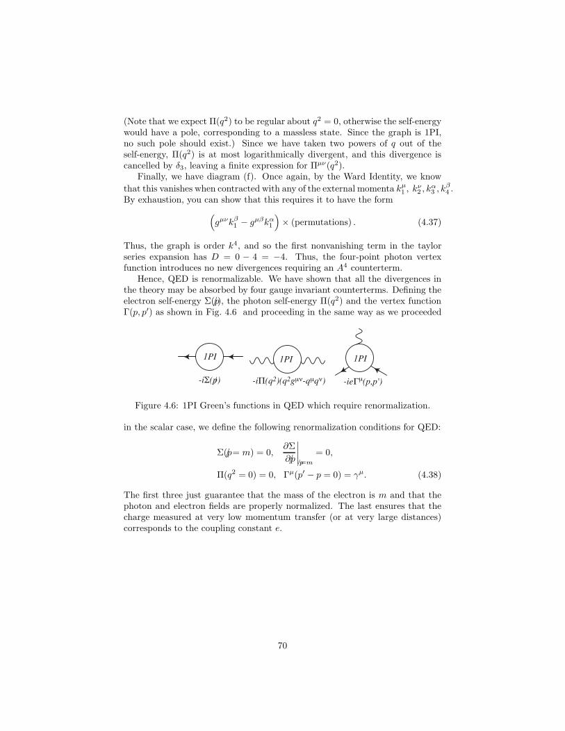
(Note that we expect Π(q2) to be regular about q2 = 0, otherwise the self-energywould have a pole, corresponding to a massless state. Since the graph is 1PI,no such pole should exist.) Since we have taken two powers of q out of theself-energy, Π(q2) is at most logarithmically divergent, and this divergence iscancelled by δ3, leaving a finite expression for Πµν(q2).

Finally, we have diagram (f). Once again, by the Ward Identity, we know

that this vanishes when contracted with any of the external momenta kµ1 , kν2 , k

α3 , k

β4 .

By exhaustion, you can show that this requires it to have the form

(

gµνkβ1 − gµβkα1

)

× (permutations) . (4.37)

Thus, the graph is order k4, and so the first nonvanishing term in the taylorseries expansion has D = 0 − 4 = −4. Thus, the four-point photon vertexfunction introduces no new divergences requiring an A4 counterterm.

Hence, QED is renormalizable. We have shown that all the divergences inthe theory may be absorbed by four gauge invariant counterterms. Defining theelectron self-energy Σ(p/), the photon self-energy Π(q2) and the vertex functionΓ(p, p′) as shown in Fig. 4.6 and proceeding in the same way as we proceeded

1PI1PI 1PI

-iΠ(q2)(q2gµν-qµqν) -ieΓµ(p,p')-iΣ(p)/

Figure 4.6: 1PI Green’s functions in QED which require renormalization.

in the scalar case, we define the following renormalization conditions for QED:

Σ(p/ = m) = 0,∂Σ

∂p/

∣

∣

∣

∣

p/=m

= 0,

Π(q2 = 0) = 0, Γµ(p′ − p = 0) = γµ. (4.38)

The first three just guarantee that the mass of the electron is m and that thephoton and electron fields are properly normalized. The last ensures that thecharge measured at very low momentum transfer (or at very large distances)corresponds to the coupling constant e.

70