photometric stereo, shape from shading sfs f&p ch 5 (old
TRANSCRIPT

Photometric Stereo, Shape from Shading SfS
F&P Ch 5 (old) Ch 2 (new)Guido Gerig
CS 6320, Spring 2015
Credits: M. Pollefey UNC CS256, Ohad Ben-Shahar CS BGU, Wolff JUN (http://www.cs.jhu.edu/~wolff/course600.461/week9.3/index.htm)

Photometric Stereo
Depth from Shading?
First step: Surface Normals from Shading
Second step: Re-integration ofsurface from Normals
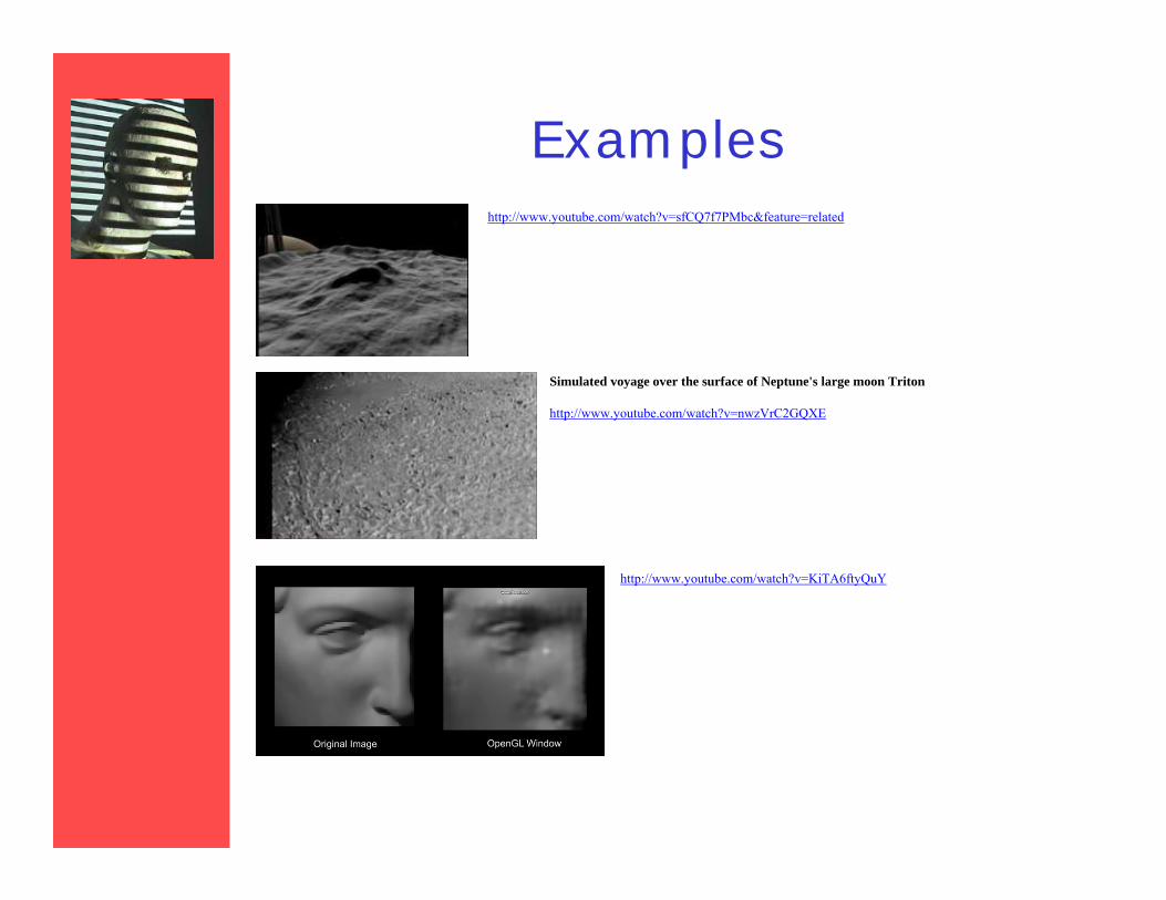
Exampleshttp://www.youtube.com/watch?v=sfCQ7f7PMbc&feature=related
http://www.youtube.com/watch?v=KiTA6ftyQuY
Simulated voyage over the surface of Neptune's large moon Triton
http://www.youtube.com/watch?v=nwzVrC2GQXE

Credit: Ohad Ben-Shahar CS BGU

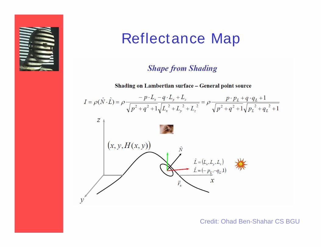
Shape from Shading
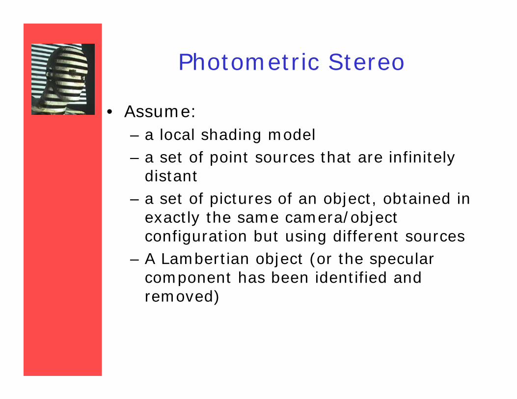
Photometric Stereo
• Assume:– a local shading model– a set of point sources that are infinitely
distant– a set of pictures of an object, obtained in
exactly the same camera/object configuration but using different sources
– A Lambertian object (or the specular component has been identified and removed)

Setting for Photometric Stereo
Multiple images with different lighting (vsbinocular/geometric stereo)

Goal: 3D from One View and multiple Source positions
Input images Usable DataMask

Scene Results
Needle Diagram:Surface Normals
Albedo
Re-lit:

Projection model for surface recovery -usually called a Monge patch

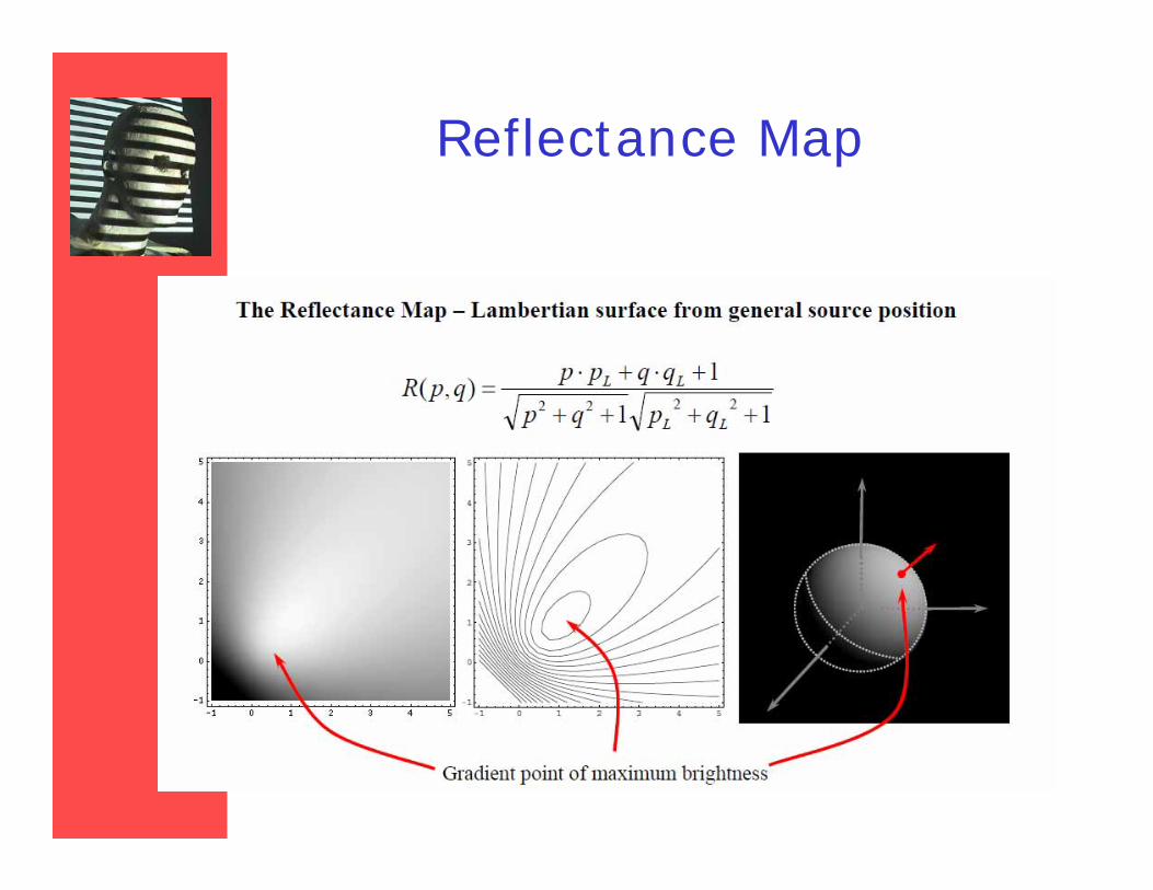
Lambertian Reflectance Map
LAMBERTIAN MODEL
E = <n,ns> =COS Y
XZ
(ps,qs,-1)
(p,q,-1)
2222 11
1
LL
LL
qpqp
qqppCOS

Wolff, November 4, 1998 12
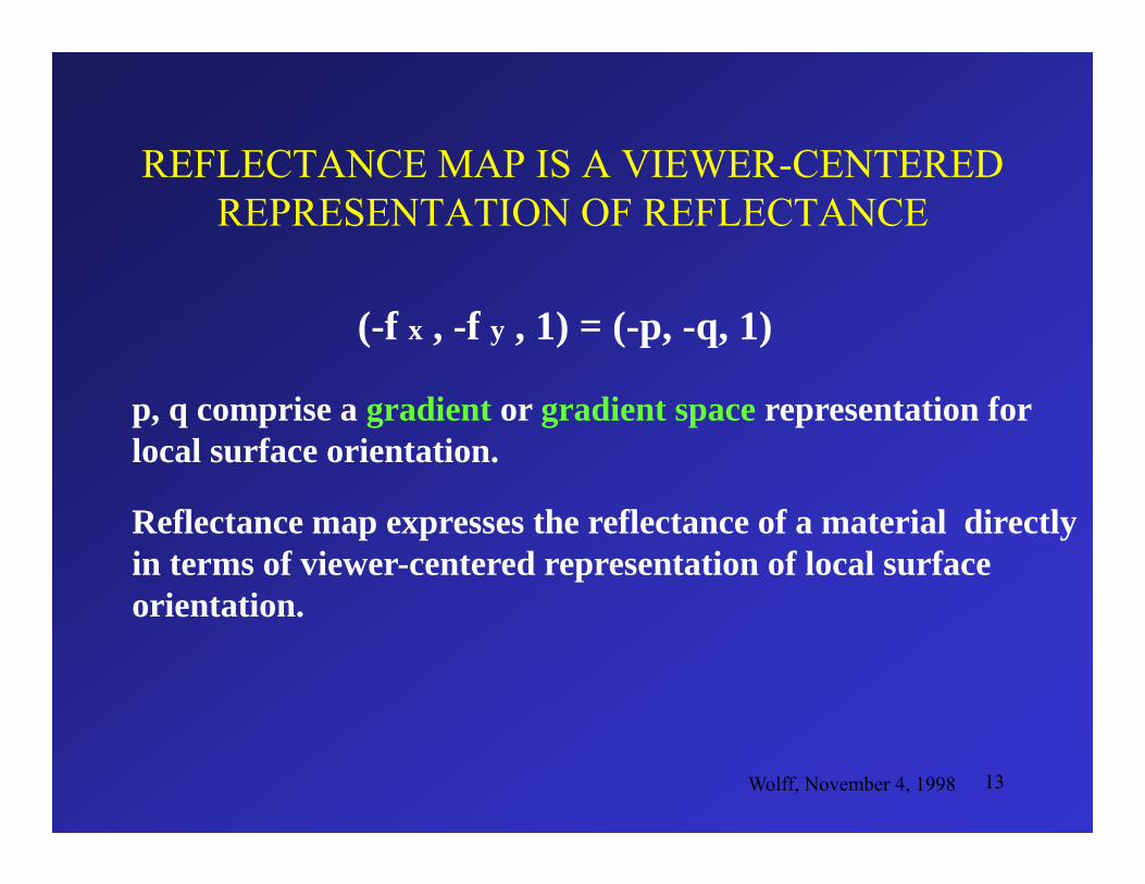
REFLECTANCE MAP IS A VIEWER-CENTERED REPRESENTATION OF REFLECTANCE
Depth
SurfaceOrientation
Y
X
Z
IMAGE PLANE
z=f(x,y)
x y
dxdy
y(-f , -f , 1)
(f , f , -1)
(0,1,f )x
(0,1,f )x
(1,0,f )
(1,0,f )y=
x y
13
REFLECTANCE MAP IS A VIEWER-CENTERED REPRESENTATION OF REFLECTANCE
(-f x , -f y , 1) = (-p, -q, 1)
p, q comprise a gradient or gradient space representation forlocal surface orientation.
Reflectance map expresses the reflectance of a material directly in terms of viewer-centered representation of local surface orientation.
Wolff, November 4, 1998

Reflectance Map (ps=0, qs=0)

Reflectance Map
Credit: Ohad Ben-Shahar CS BGU
Reflectance Map
Credit: Ohad Ben-Shahar CS BGU
Reflectance Map
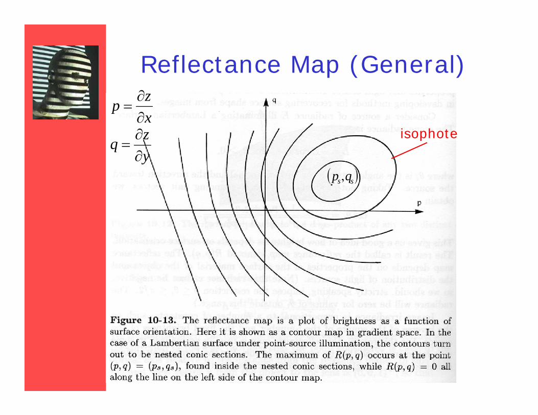
Reflectance Map (General)
yzq
xzp
isophote
ss qp ,

Reflectance Map
Given Intensity I in image, there are multiple (p,q) combinations (= surface orientations).
Use multiple images with different light source directions.
yzq
xzp
Isophote I
ss qp ,
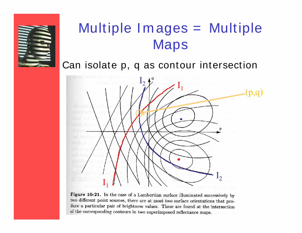
Multiple Images = Multiple Maps
Can isolate p, q as contour intersection
(p,q)I1
I2
I2I1

Example: Two Views
Still not unique for certain intensity pairs.
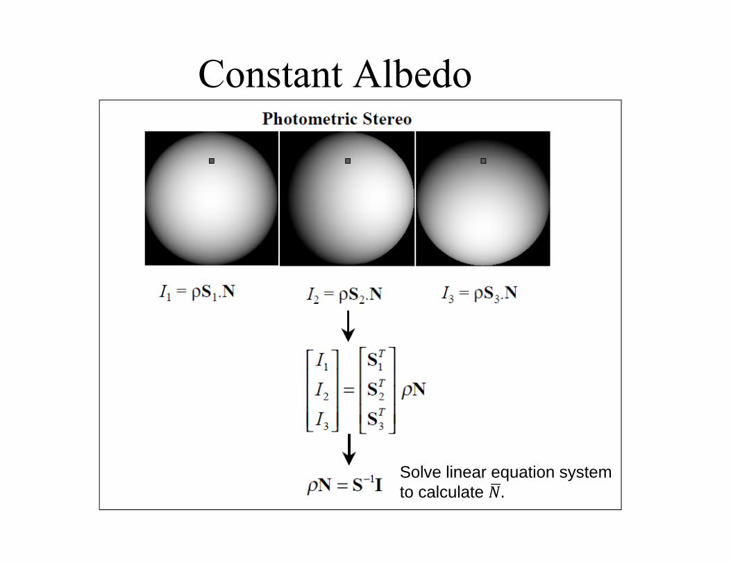
Constant Albedo
Solve linear equation systemto calculate .
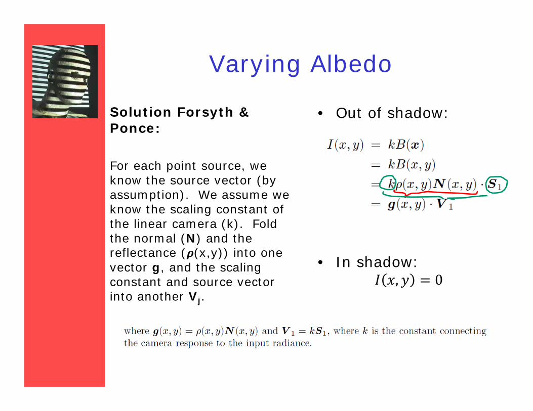
Varying Albedo
Solution Forsyth & Ponce:
For each point source, we know the source vector (by assumption). We assume we know the scaling constant of the linear camera (k). Fold the normal (N) and the reflectance ( (x,y)) into one vector g, and the scaling constant and source vector into another Vj.
• Out of shadow:
• In shadow:, 0

Multiple Images:Linear Least Squares Approach• Combine albedo and normal• Separate lighting parameters• More than 3 images => overdetermined system
• How to calculate albedo and ?̅ , , (x,y)
→ = , , ̅
: ̅(x,y)= i(x,y)

Example LLS Input
Problem: Some regions in some images are in the shadow (no image intensity).

Dealing with Shadows (Missing Info)
For each point source, we know the source vector (by assumption). We assume we know the scaling constant of the linear camera. Fold the normal and the reflectance into one vector g, and the scaling constant and source vector into another Vj
Out of shadow:
In shadow:Ij(x,y) 0
I j (x, y) kB(x, y)
k(x, y) N(x, y)S j g(x,y)Vj
No partial shadow

Matrix Trick for Complete Shadows
• Matrix from Image Vector:
• Multiply LHS and RHS with diag matrix
I 12 ( x , y )
I 22 ( x , y )
..I n
2 ( x , y )
I 1 ( x , y ) 0 .. 00 I 2 ( x , y ) .. .... .. .. 00 .. 0 I n ( x , y )
V1T
V 2T
..V n
T
g ( x , y )
Known Known KnownUnknown
Relevant elements of the left vector and the matrix are zero at points that are in shadow.
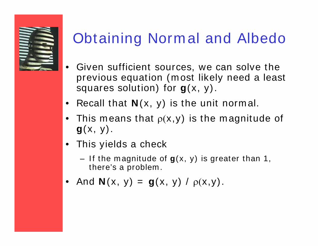
Obtaining Normal and Albedo
• Given sufficient sources, we can solve the previous equation (most likely need a least squares solution) for g(x, y).
• Recall that N(x, y) is the unit normal.• This means that x,y) is the magnitude of
g(x, y).• This yields a check
– If the magnitude of g(x, y) is greater than 1, there’s a problem.
• And N(x, y) = g(x, y) / x,y).
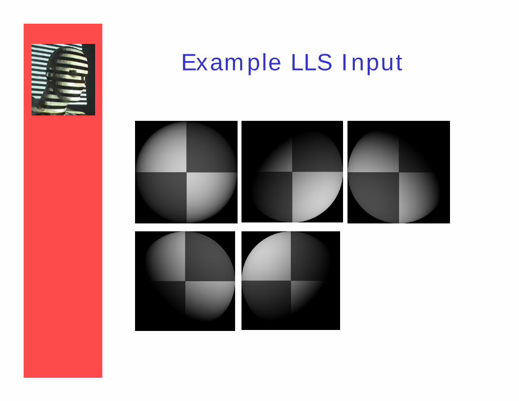
Example LLS Input
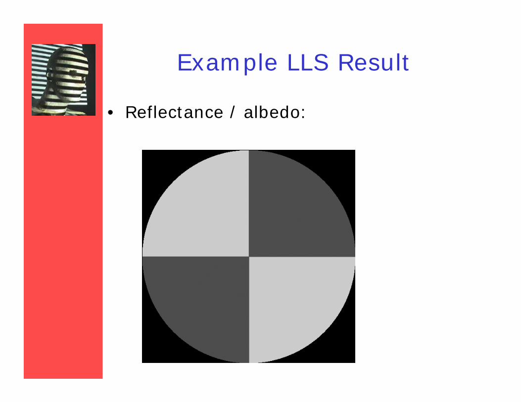
Example LLS Result
• Reflectance / albedo:

Recap
• Obtain normal / orientation, no depth
IMAGE PLANE
Depth?
SurfaceOrientation
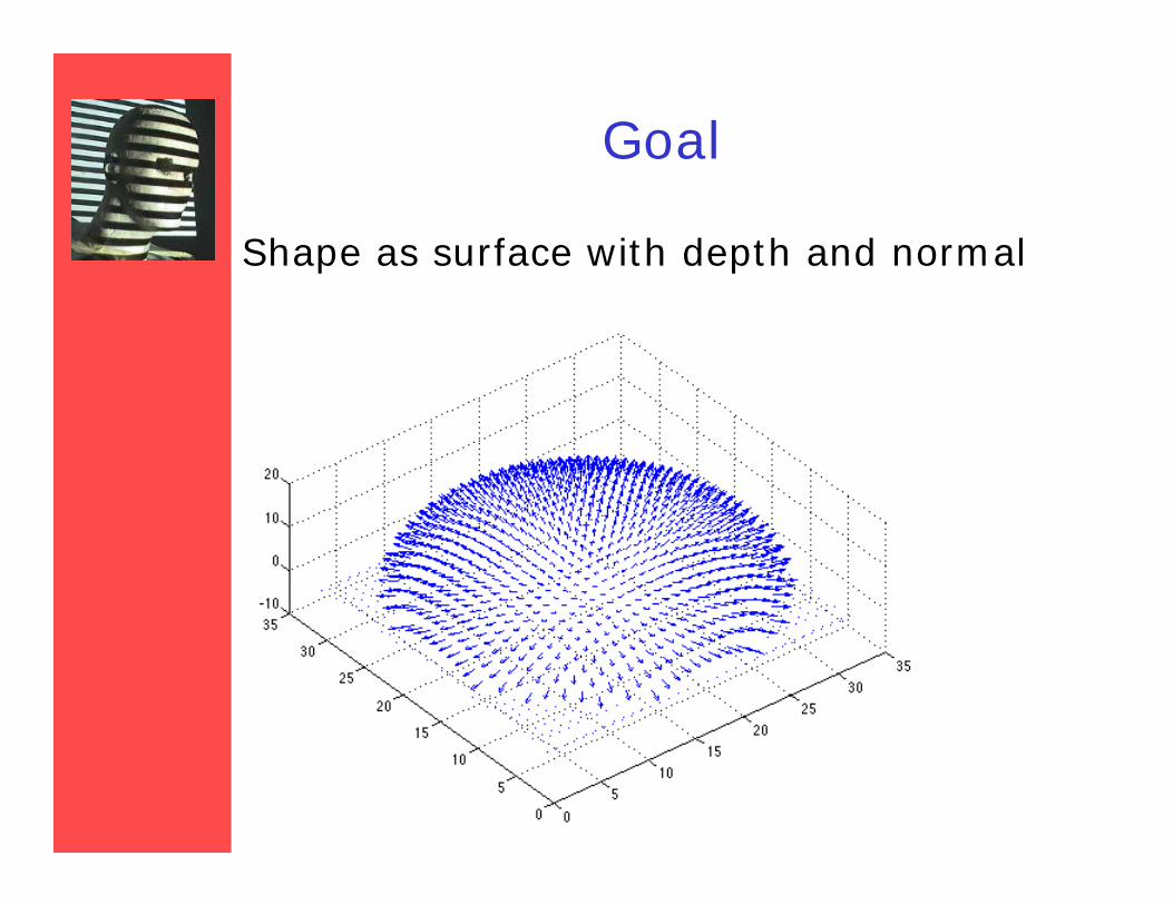
Goal
Shape as surface with depth and normal
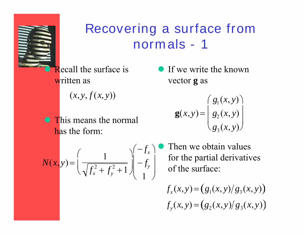
Recovering a surface from normals - 1
Recall the surface is written as
This means the normal has the form:
If we write the known vector g as
Then we obtain values for the partial derivatives of the surface:
(x,y, f (x, y))
g(x,y) g1(x, y)g2 (x, y)g3(x, y)
fx (x,y) g1(x, y) g3(x, y) fy(x, y) g2(x,y) g3(x,y)
N(x,y) 1
fx2 fy
2 1
fx
fy
1

Recovering a surface from normals - 2
Recall that mixed second partials are equal --- this gives us an integrabilitycheck. We must have:
We can now recover the surface height at any point by integration along some path, e.g.
g1(x, y) g3(x, y) y
g2(x, y) g3(x, y) x
f (x, y) fx (s, y)ds0
x
fy (x,t)dt0
y
c

Height Map from Integration
How to integrate?

Possible Solutions
• Engineering approach: Path integration (Forsyth & Ponce)
• In general: Calculus of Variation Approaches
• Horn: Characteristic Strip Method• Kimmel, Siddiqi, Kimia, Bruckstein: Level
set method• Many others ….

Shape by Integation (Forsyth&Ponce)• The partial derivative gives the change in surface height
with a small step in either the x or the y direction• We can get the surface by summing these changes in
height along some path.

Simple Algorithm Forsyth & Ponce
Problem: Noise and numerical (in)accuracy are added up and result in distorted surface.
Solution: Choose several different integration paths, and build average height map.
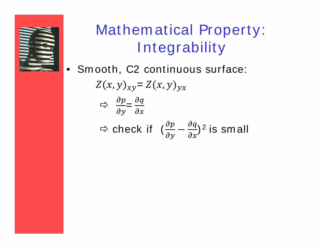
Mathematical Property: Integrability
• Smooth, C2 continuous surface:=
=
check if ( )2 is small

Wolff, November 4, 1998
SHAPE FROM SHADING(Calculus of Variations Approach)
• First Attempt: Minimize error in agreement with Image Irradiance Equation over the region of interest:
( ( , ) ( , ))I x y R p q dxdyobject
2

SHAPE FROM SHADING(Calculus of Variations Approach)
• Better Attempt: Regularize the Minimization oferror in agreement with Image Irradiance Equationover the region of interest:
p p q q I x y R p q dxdyx y x y
object
2 2 2 2 2 ( ( , ) ( , ))
Wolff, November 4, 1998
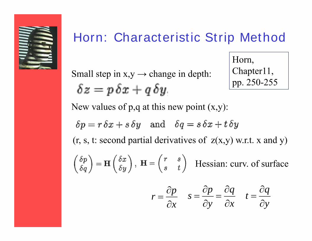
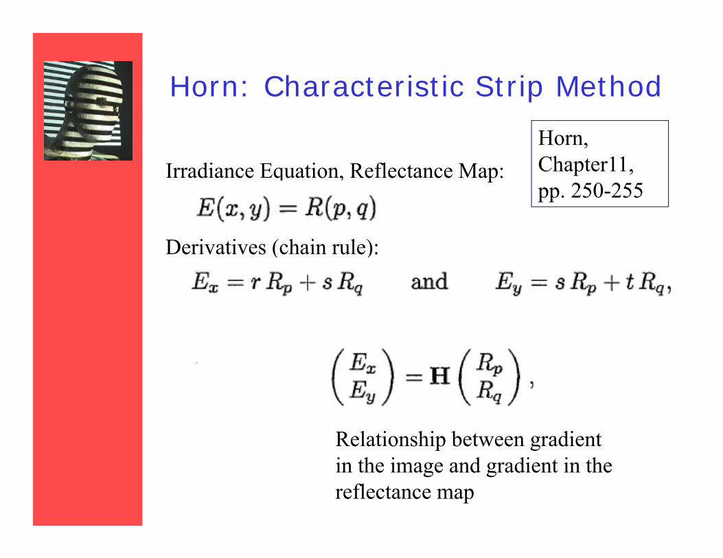
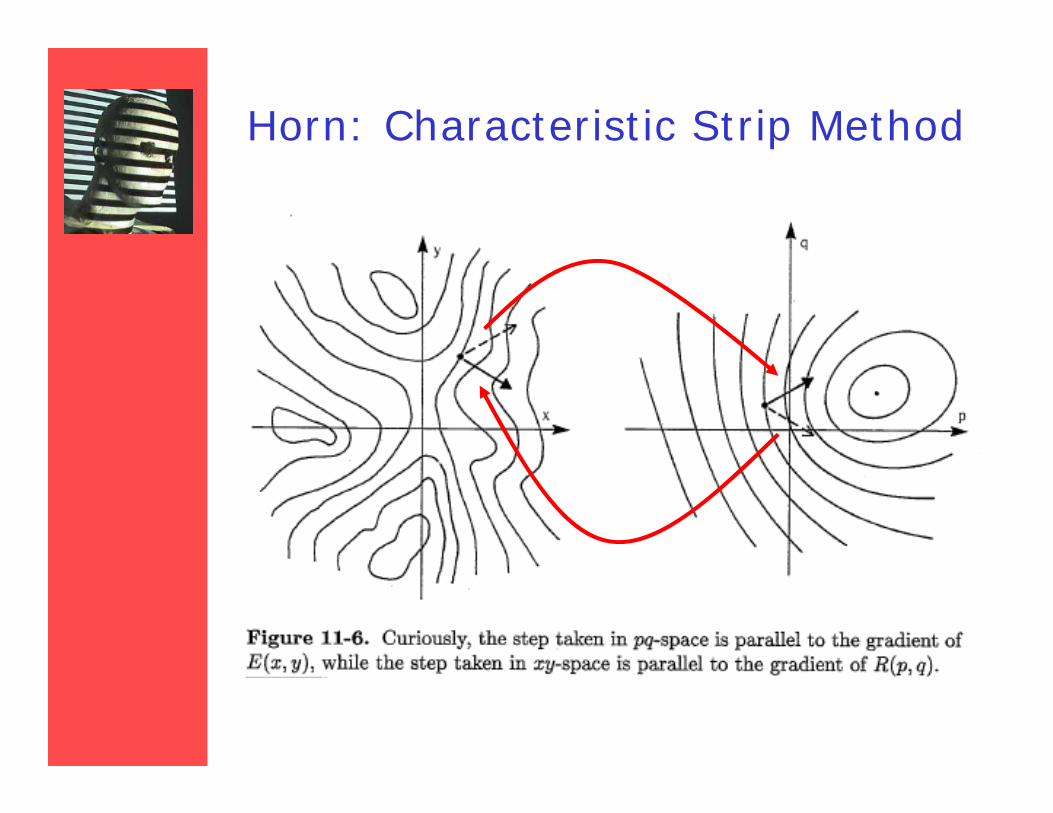
Horn: Characteristic Strip Method Horn, Chapter11, pp. 250-255
Small step in x,y → change in depth:
New values of p,q at this new point (x,y):
(r, s, t: second partial derivatives of z(x,y) w.r.t. x and y)
Hessian: curv. of surface
xpr
xq
yps
yqt
Horn: Characteristic Strip Method Horn, Chapter11, pp. 250-255
Irradiance Equation, Reflectance Map:
Derivatives (chain rule):
Relationship between gradient in the image and gradient in the reflectance map
Horn: Characteristic Strip Method Horn, Chapter11, pp. 250-255
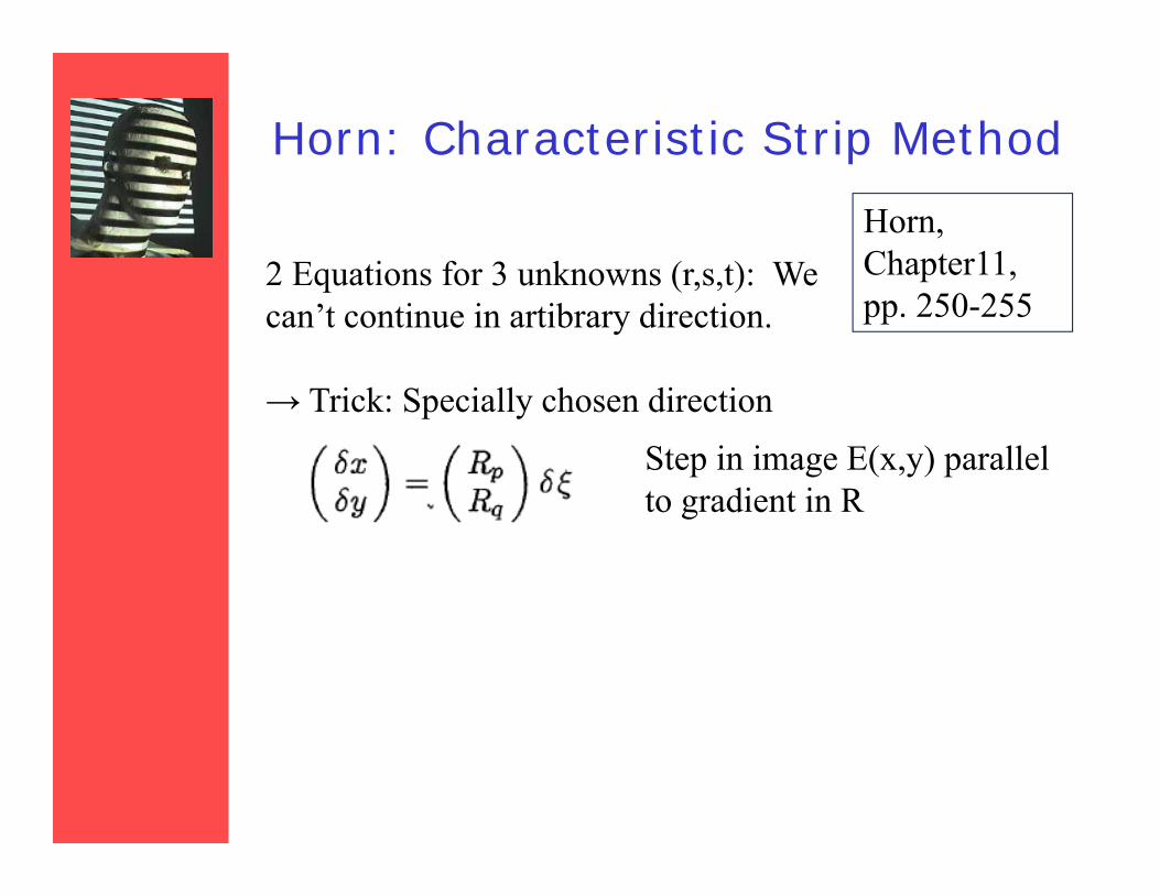
2 Equations for 3 unknowns (r,s,t): We can’t continue in artibrary direction.
→ Trick: Specially chosen direction
Step in image E(x,y) parallel to gradient in R

Horn: Characteristic Strip Method Horn, Chapter11, pp. 250-255
2 Equations for 3 unknowns (r,s,t): We can’t continue in artibrary direction.
→ Trick: Specially chosen direction
Step in image E(x,y) parallel to gradient in R
Solving for new values for p,q:
Change in (p,q) can be computed via gradient of image
Horn: Characteristic Strip Method

Horn: Characteristic Strip Method
Solution of differential equations: Curve on surface

Horn: Characteristic Strip Method

Horn: Characteristic Strip Method
Horn, Chapter11, pp. 250-255

Another Solution to SFS:Kimmel, Siddiqi, Kimia, Bruckstein
xpdf document

Kimmel, Siddiqi, Kimia, Bruckstein
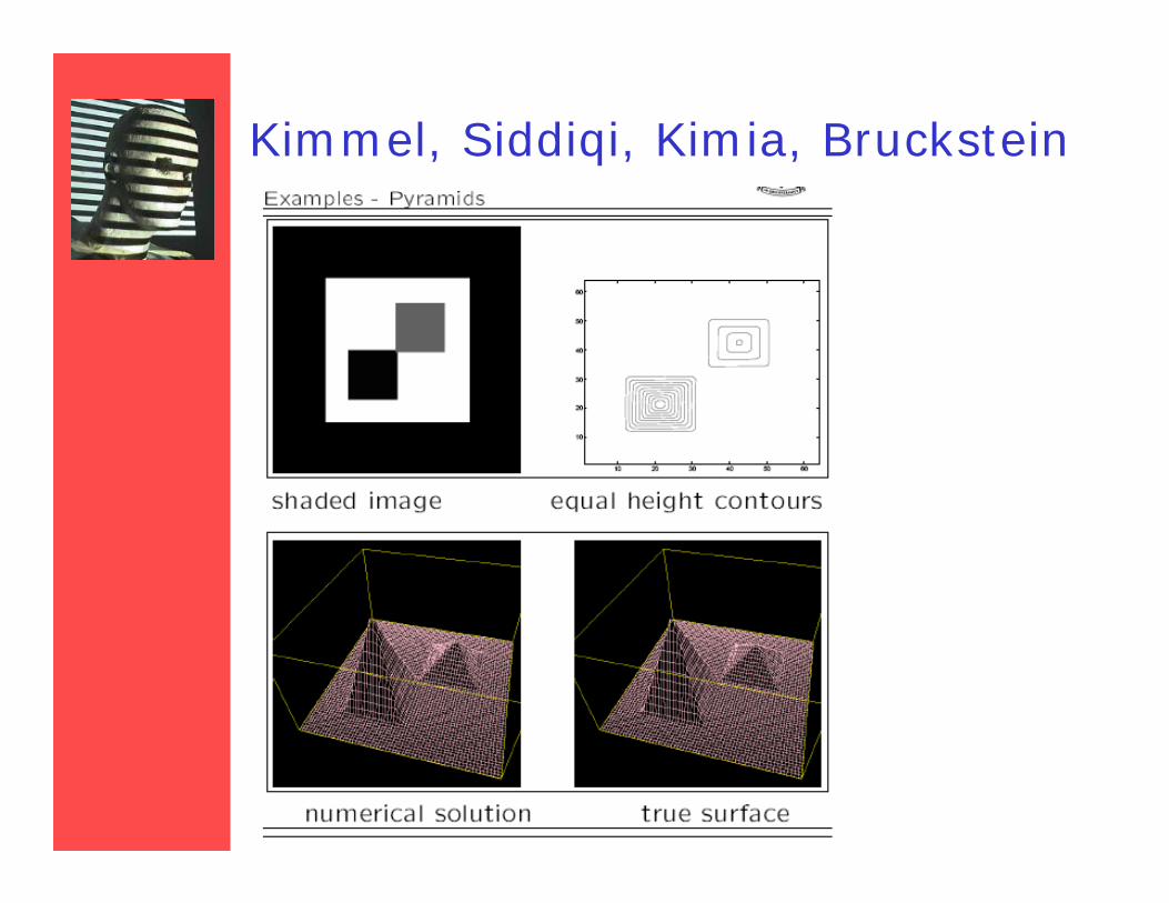
Kimmel, Siddiqi, Kimia, Bruckstein

Kimmel, Siddiqi, Kimia, Bruckstein

Application Area: Geography

Application: Braille Code
pdf document

Mars Rover Heads to a New Crater NYT Sept 22, 2008

Limitations
• Controlled lighting environment– Specular highlights?– Partial shadows?– Complex interrreflections?
• Fixed camera– Moving camera?– Multiple cameras?
=> Another approach: binocular / geometric stereo