photoelectron spectroscopy - fhi · handbook of photoelectron spectroscopy etc.*) • clean...
TRANSCRIPT

Modern Methods in Heterogeneous Catalysis
Research
Photoelectron Spectroscopy
Axel Knop ([email protected])
Outline
Photoelectron Spectroscopy: General Principle
Surface sensitivity
Instrumentation
Background subtraction
PES peaks, loss features
Binding energy calibrationBinding energy calibration
Chemical state
Peak fitting
Quantitative Analysis
High pressure XPS
examples

Problem: What is the (chemical) composition of a surface
Me0 Me2+
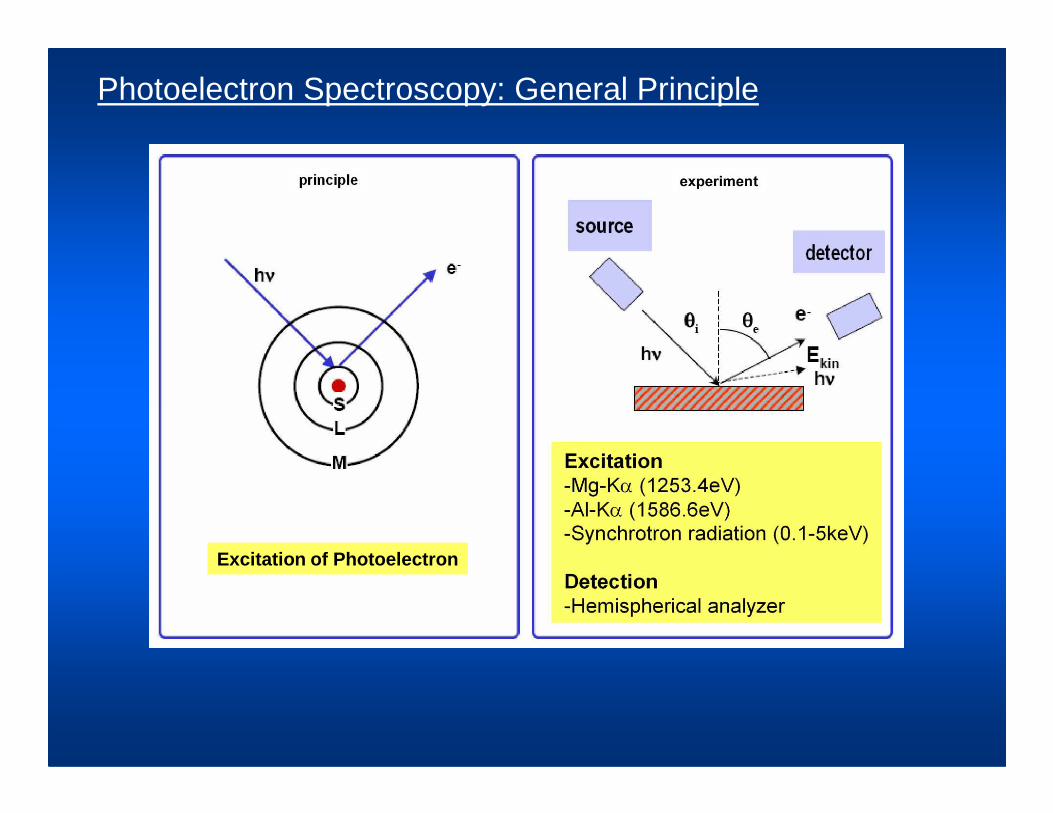
Photoelectron Spectroscopy: General Principle
Excitation of Photoelectron
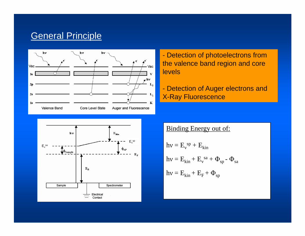
General Principle
- Detection of photoelectrons from the valence band region and core levels
- Detection of Auger electrons and X-Ray Fluorescence
Binding Energy out of:
hν = Evsp + Ekin
hν = Ekin + Evsa+ Φsp - Φsa
hν = Ekin + EF + Φsp
Evsa
Evsp
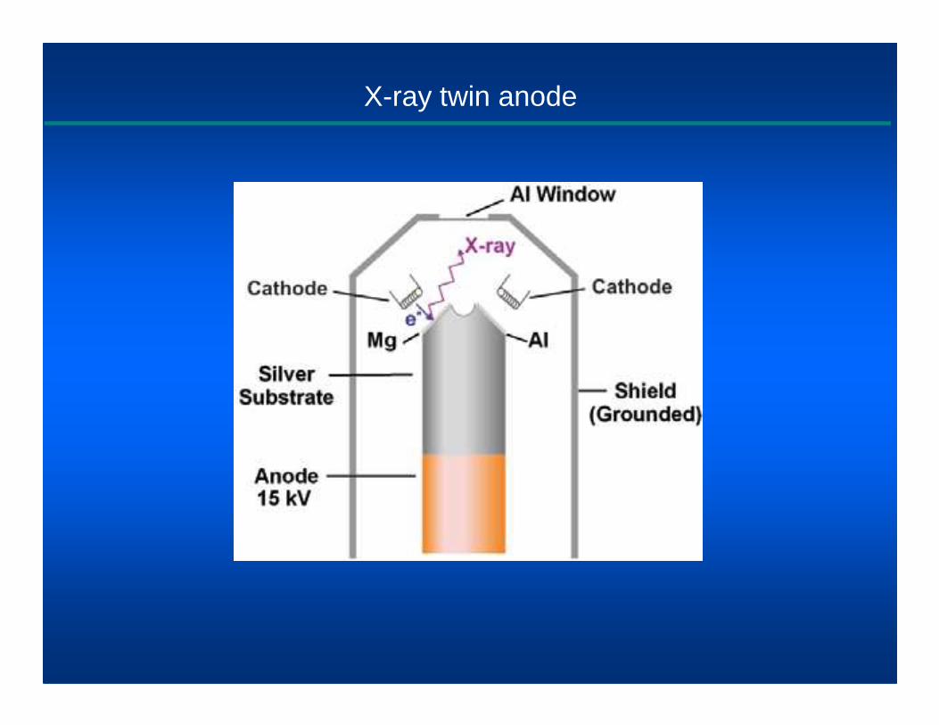
X-ray twin anode

Parallel plate mirror analyser

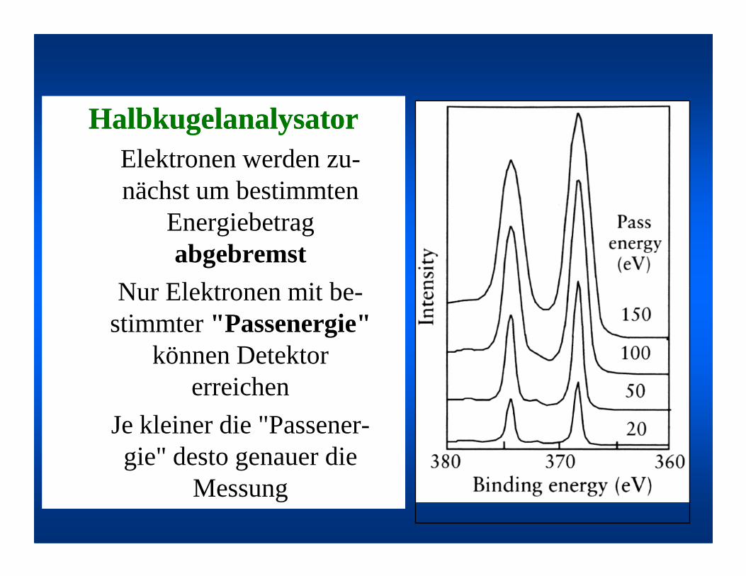
HalbkugelanalysatorHalbkugelanalysatorElektronen werden zu-nächst um bestimmten
Energiebetragabgebremst
Nur Elektronen mit be-Nur Elektronen mit be-stimmter"Passenergie"
können Detektorerreichen
Je kleiner die "Passener-gie" desto genauer die
Messung
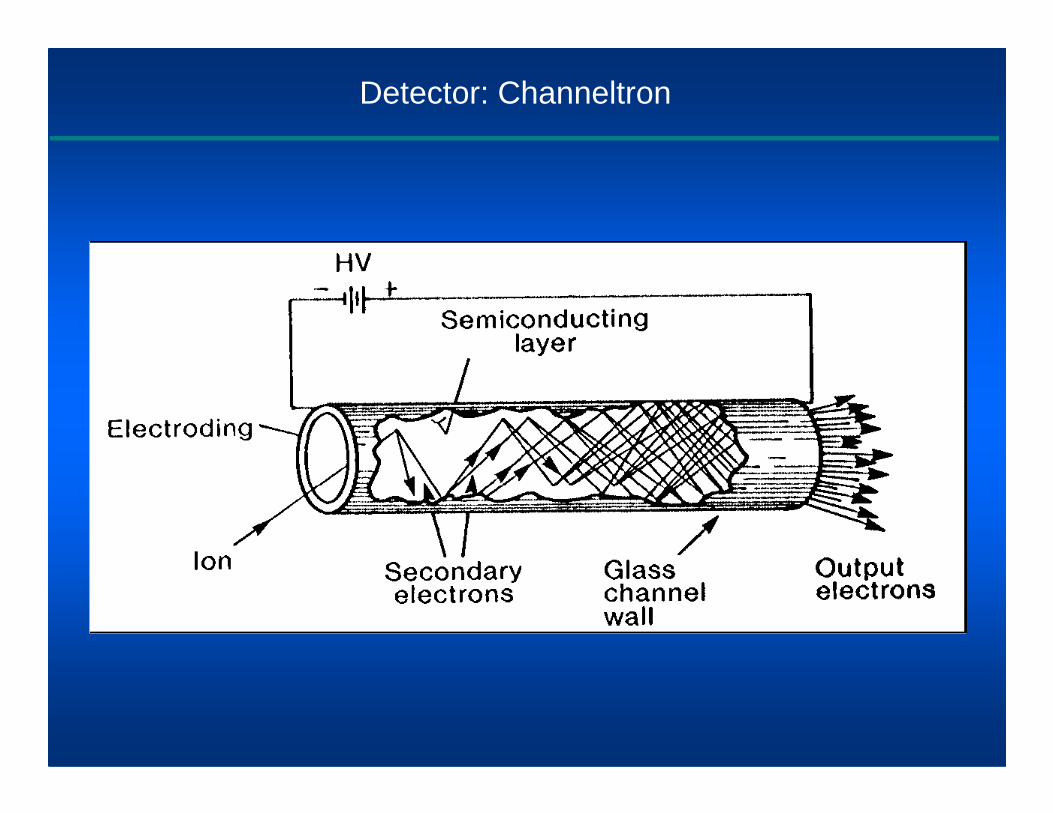
Detector: Channeltron

XP spectra: two different anode materials

Where do the electrons come from?
Distance electron can travel in solids depends on:
• Material• Electron kinetic energy
� Measure attenuation of electrons by covering surface electrons by covering surface with known thickness of element
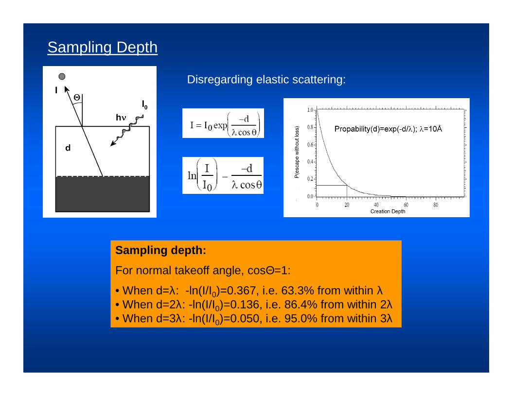
Sampling Depth
Disregarding elastic scattering:
Sampling depth:
For normal takeoff angle, cosΘ=1:
• When d=λ: -ln(I/I0)=0.367, i.e. 63.3% from within λ• When d=2λ: -ln(I/I0)=0.136, i.e. 86.4% from within 2λ• When d=3λ: -ln(I/I0)=0.050, i.e. 95.0% from within 3λ

Mean Free Path of Electrons in Solids
• IMFP is average distance between inelastic collisions• Minimum λ of 5-10Å for KE ~ 50-100 eV� Maximum surface sensitivity

Origin of background
Background of scattered electrons due to limited IMFP� Higher for low KE
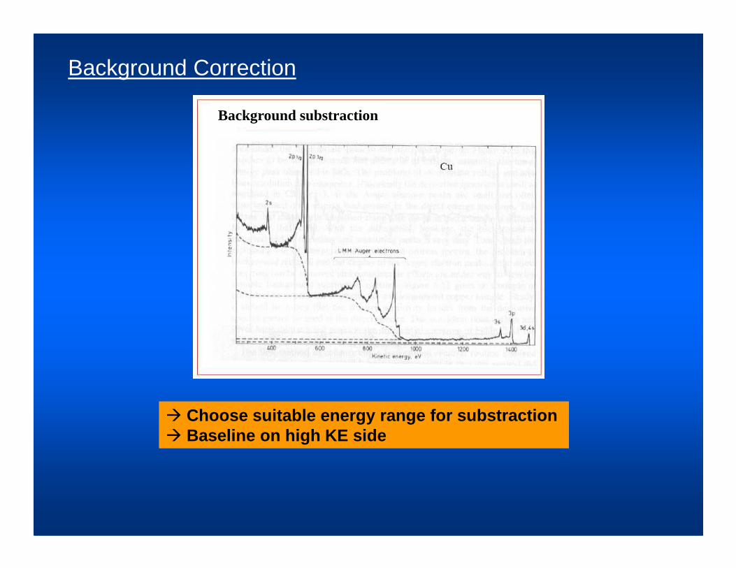
Background Correction
Background substraction
� Choose suitable energy range for substraction� Baseline on high KE side

Background Correction
Several ways to substract background:
- Stepwise- Linear- Method of Tougaard
�Most common:
Method of Shirley et al.:
worst
Always use same background substraction method for all peaks!
D.A. Shirley, Phys. Rev. B, 5, S. 4709, 1972.
best
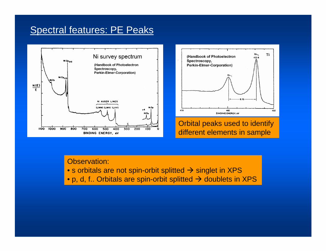
Spectral features: PE Peaks
Orbital peaks used to identify Orbital peaks used to identify different elements in sample
Observation: • s orbitals are not spin-orbit splitted � singlet in XPS• p, d, f.. Orbitals are spin-orbit splitted � doublets in XPS

Spectral features: PE Peaks
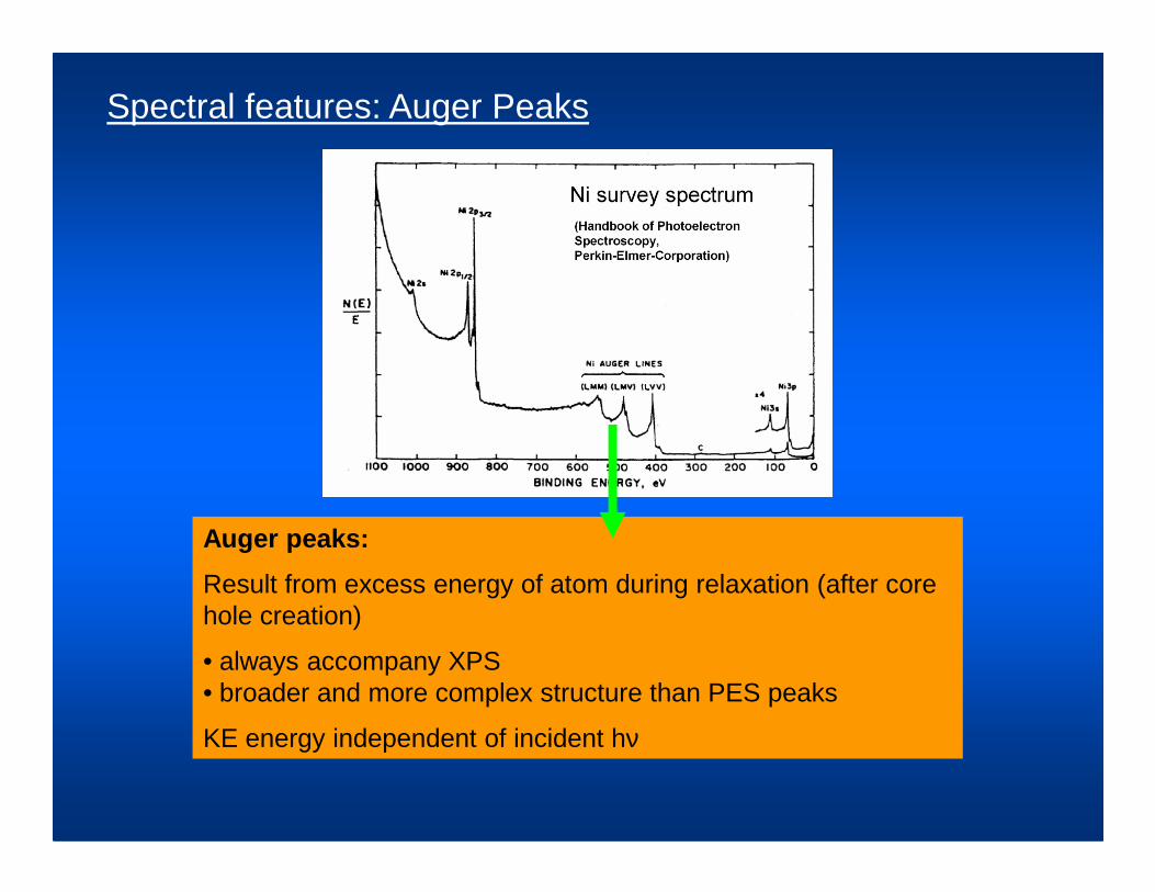
Spectral features: Auger Peaks
Auger peaks:
Result from excess energy of atom during relaxation (after core hole creation)
• always accompany XPS• broader and more complex structure than PES peaks
KE energy independent of incident hν
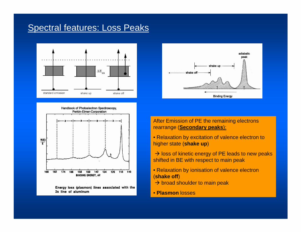
Spectral features: Loss Peaks
After Emission of PE the remaining electrons rearrange (Secondary peaks ):
• Relaxation by excitation of valence electron to higher state (shake up )
� loss of kinetic energy of PE leads to new peaks shifted in BE with respect to main peak
• Relaxation by ionisation of valence electron (shake off )� broad shoulder to main peak
• Plasmon losses
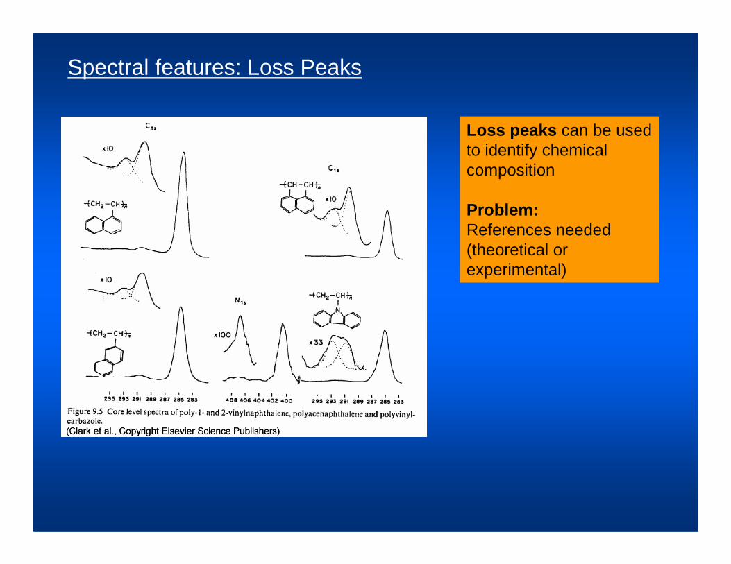
Spectral features: Loss Peaks
Loss peaks can be used to identify chemical composition
Problem:References needed (theoretical or experimental)

Relationship between the degree of core level asymmetry and the density of states at the Fermi
level (BE=0)

Analyzing the data: Calibration of Binding Energies
Identification of FE:
Easy for high density of states near EF, but may be ambigeous for samples with low DOS near EF, band gap or charged samples

Line profile modification by charging
Mo oxide on silica
real catalyst is powder sample after impregnation and calcination.and calcination.
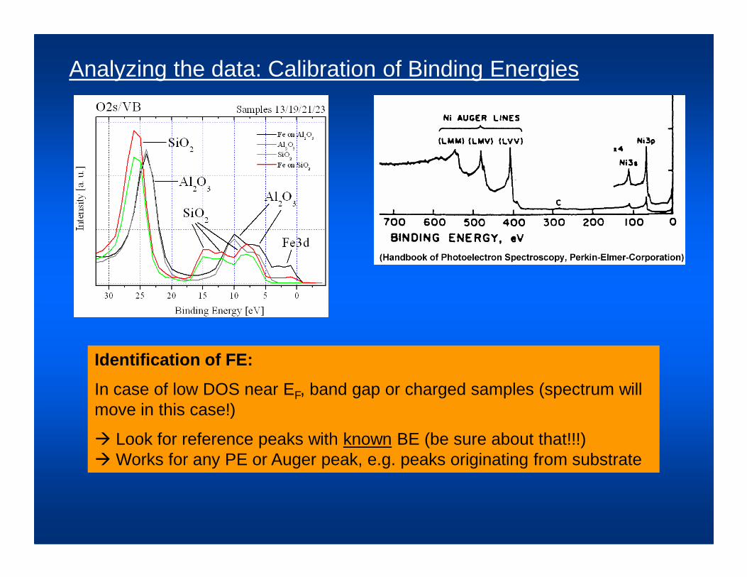
Analyzing the data: Calibration of Binding Energies
Identification of FE:
In case of low DOS near EF, band gap or charged samples (spectrum will move in this case!)
� Look for reference peaks with known BE (be sure about that!!!)� Works for any PE or Auger peak, e.g. peaks originating from substrate
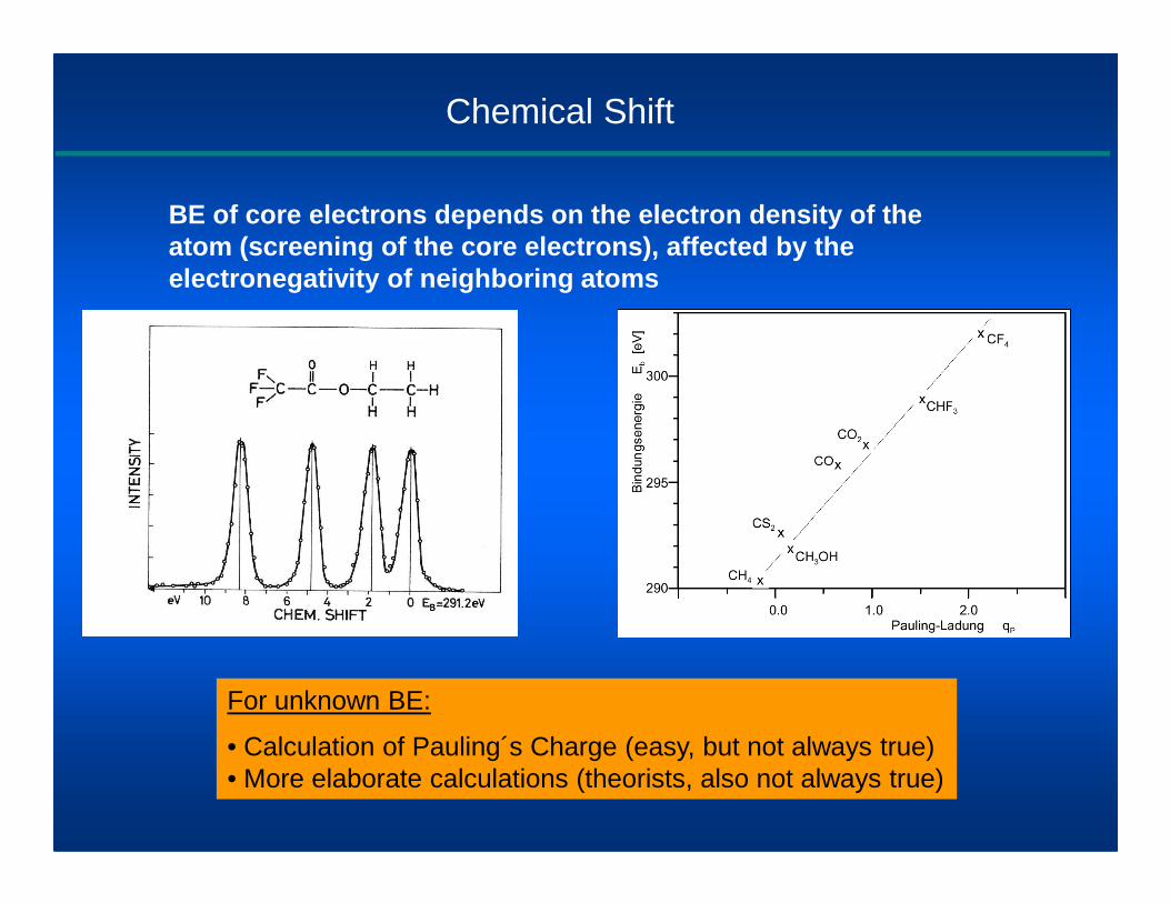
Chemical Shift
BE of core electrons depends on the electron densit y of the atom (screening of the core electrons), affected by the electronegativity of neighboring atoms
For unknown BE:
• Calculation of Pauling´s Charge (easy, but not always true)• More elaborate calculations (theorists, also not always true)
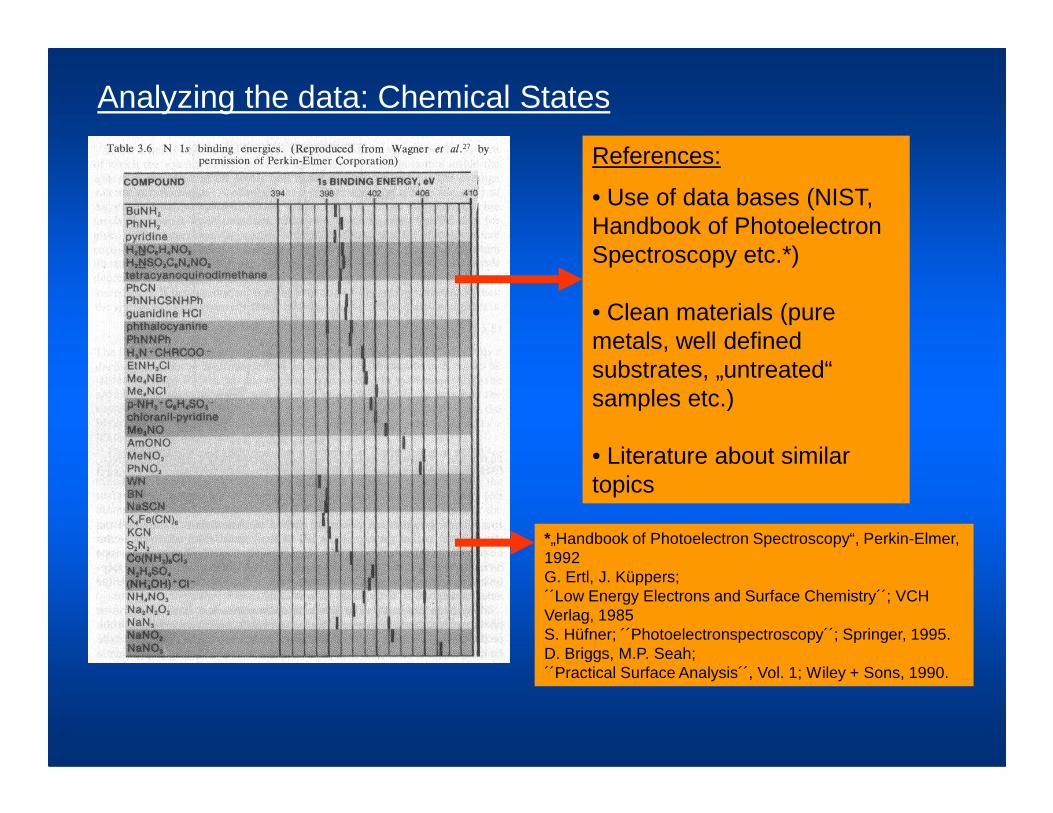
References:
• Use of data bases (NIST, Handbook of Photoelectron Spectroscopy etc.*)
• Clean materials (pure metals, well defined substrates, „untreated“ samples etc.)
Analyzing the data: Chemical States
samples etc.)
• Literature about similar topics
*„Handbook of Photoelectron Spectroscopy“, Perkin-Elmer, 1992G. Ertl, J. Küppers;´´Low Energy Electrons and Surface Chemistry´´; VCH Verlag, 1985S. Hüfner; ´´Photoelectronspectroscopy´´; Springer, 1995.D. Briggs, M.P. Seah;´´Practical Surface Analysis´´, Vol. 1; Wiley + Sons, 1990.

Analyzing the data: Peak Fitting
Several influences on peak shape:
• Broadening mainly due to excitating light (natural), structural and thermal effects
• Asymmetry due to final state effects
• Species with similar BE
These effects have to be considered when fitting by reasonable chemical/physical model of the sample!!!

Analyzing the data: Peak Fitting
Asymmetric Peak shapes modeled by
Most fitting programs provide useful tools:
Levenberg-Marquardt algorithm to minimize the χ2
M: measured spectrumN: energy valuesS: synthesized spectrumP: parameter values
β: peak parameterM: mixing ratioα: asymmetry parameter
Doniach-Sunjic functions (convoluted with Gaussian profiles)
α: asymmetry parameterh: peak heightα � 0: Lorentzian profile
Convolution of Lorentz (or D.S.) Gaussian profiles suited best!!
� Voigt function
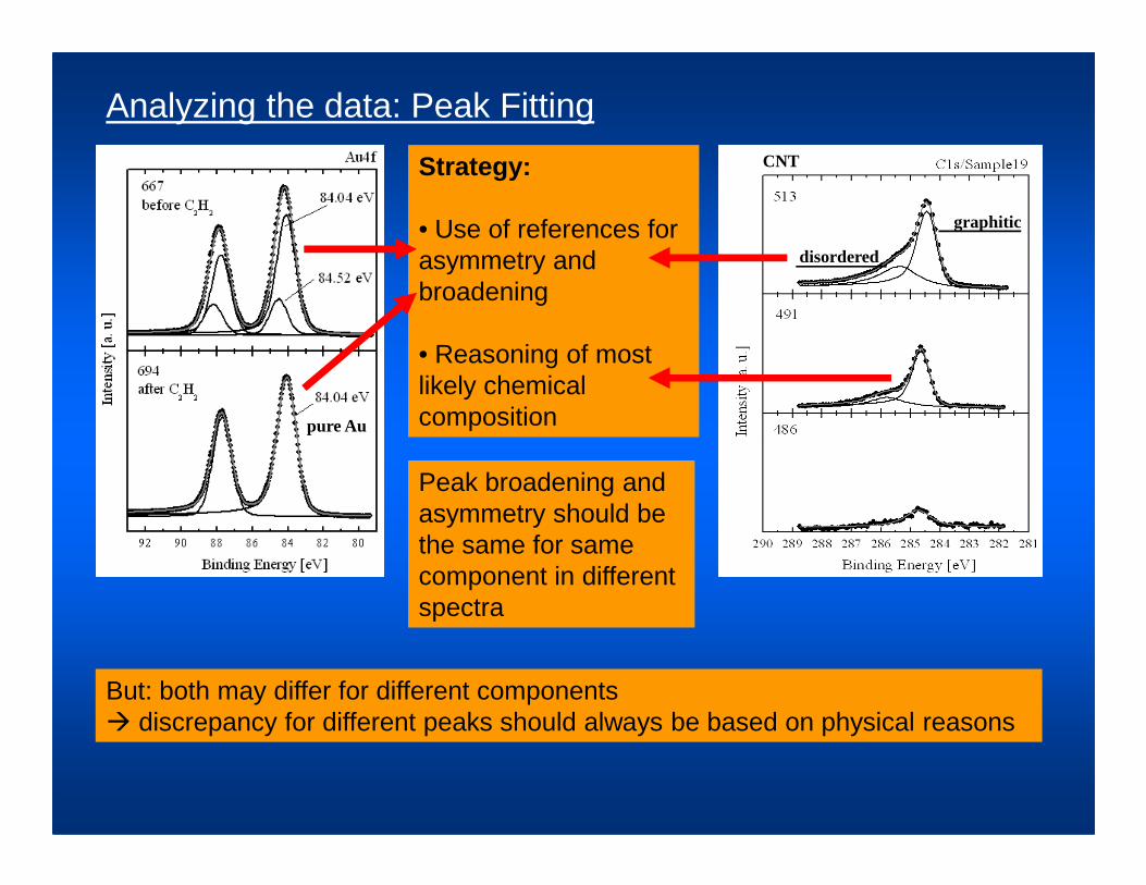
Strategy:
• Use of references for asymmetry and broadening
• Reasoning of most likely chemical composition
Analyzing the data: Peak Fitting
pure Au
graphitic
CNT
disordered
Peak broadening and asymmetry should be the same for same component in different spectra
But: both may differ for different components � discrepancy for different peaks should always be based on physical reasons
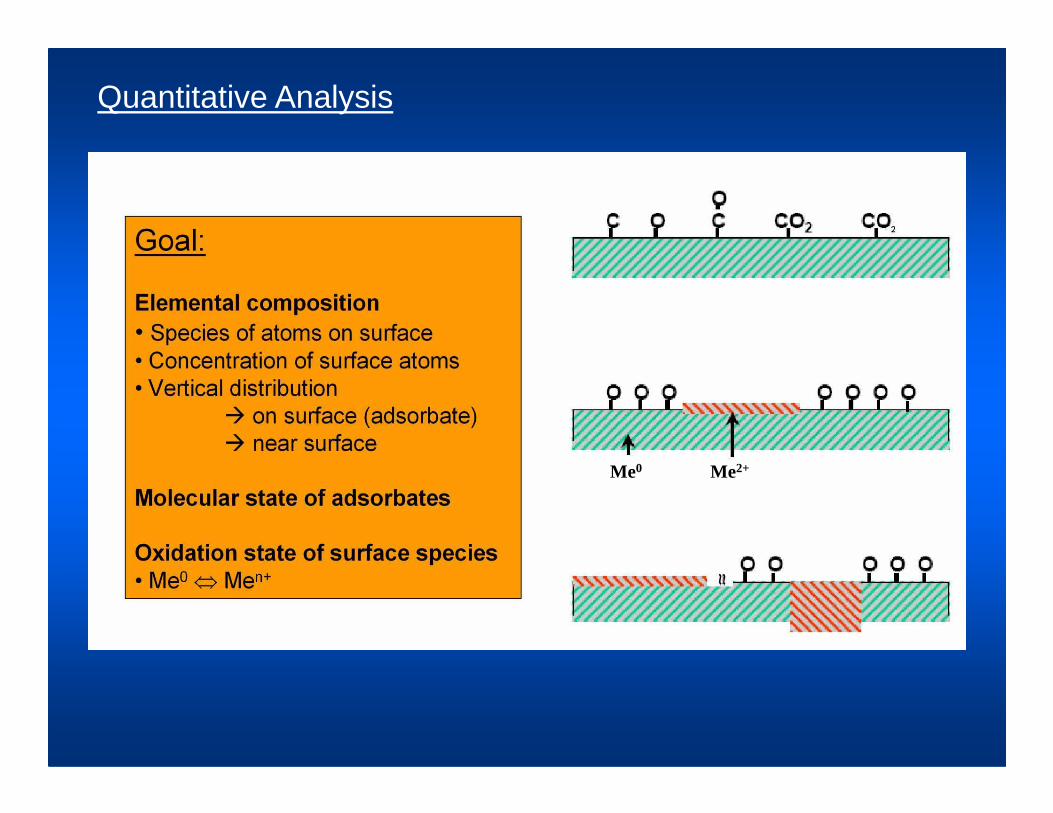
Quantitative Analysis
Me0 Me2+
Quantitative Analysis: First Steps
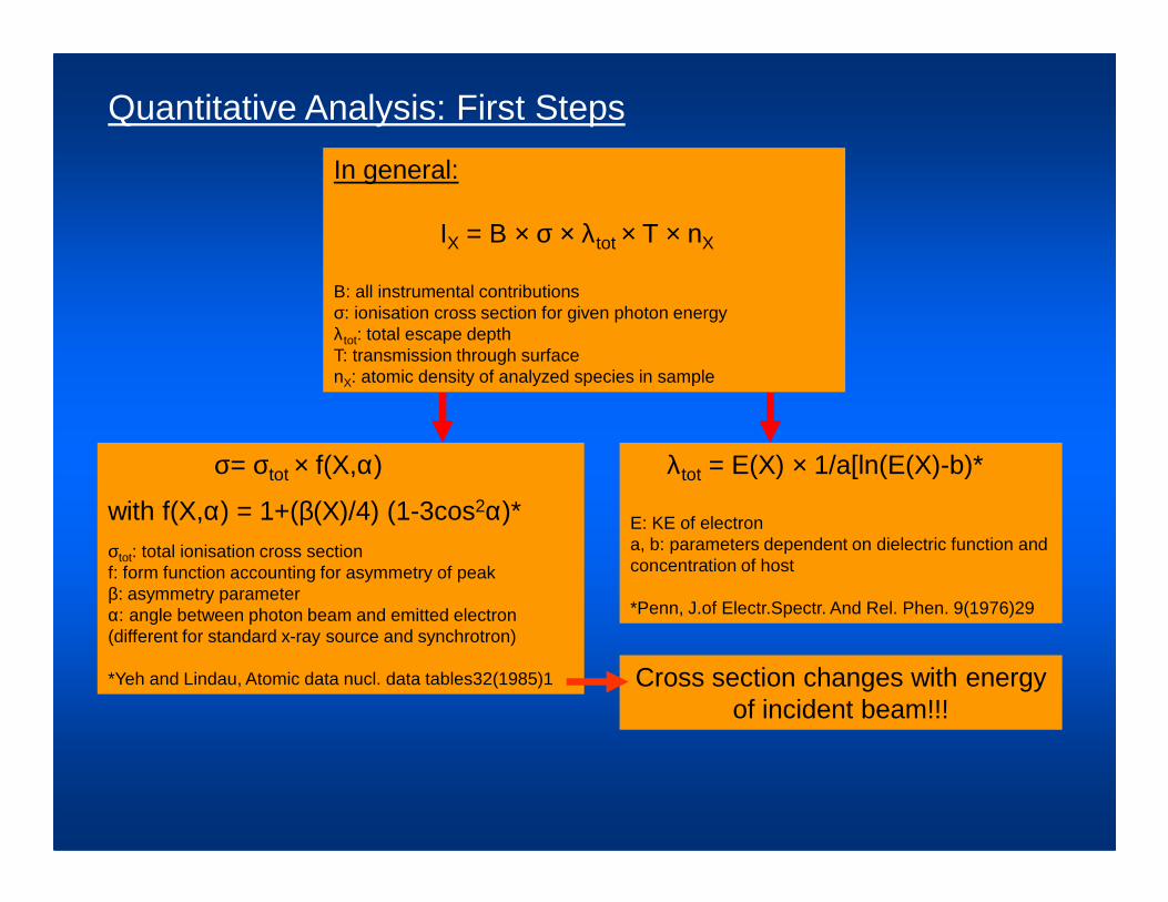
In general:
IX = B × σ × λtot × T × nX
B: all instrumental contributionsσ: ionisation cross section for given photon energyλtot: total escape depthT: transmission through surfacenX: atomic density of analyzed species in sample
σ= σ × f(X,α) λ = E(X) × 1/a[ln(E(X)-b)*σ= σtot × f(X,α)
with f(X,α) = 1+(β(X)/4) (1-3cos2α)*σtot: total ionisation cross sectionf: form function accounting for asymmetry of peakβ: asymmetry parameterα: angle between photon beam and emitted electron (different for standard x-ray source and synchrotron)
*Yeh and Lindau, Atomic data nucl. data tables32(1985)1
λtot = E(X) × 1/a[ln(E(X)-b)*
E: KE of electrona, b: parameters dependent on dielectric function and concentration of host
*Penn, J.of Electr.Spectr. And Rel. Phen. 9(1976)29
Cross section changes with energy of incident beam!!!
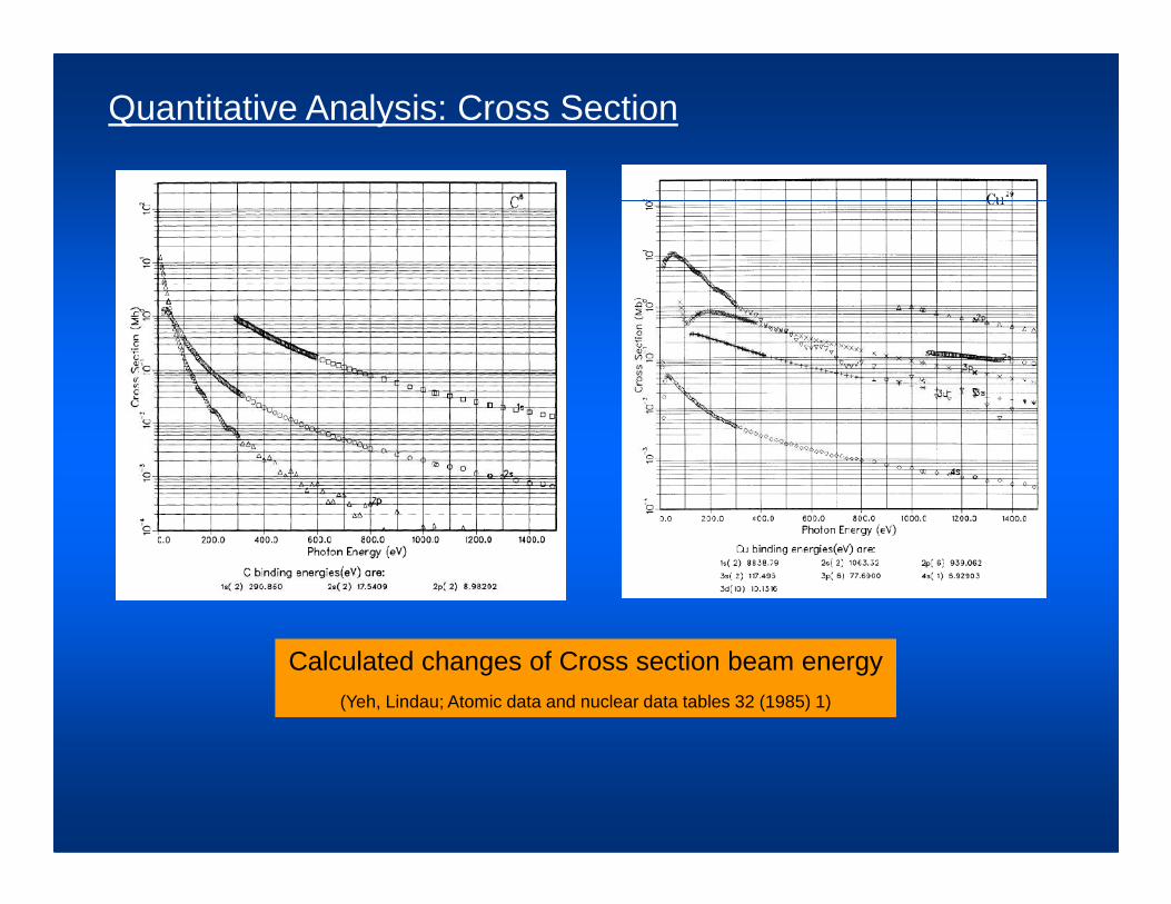
Quantitative Analysis: Cross Section
Calculated changes of Cross section beam energy(Yeh, Lindau; Atomic data and nuclear data tables 32 (1985) 1)
Quantitative Analysis
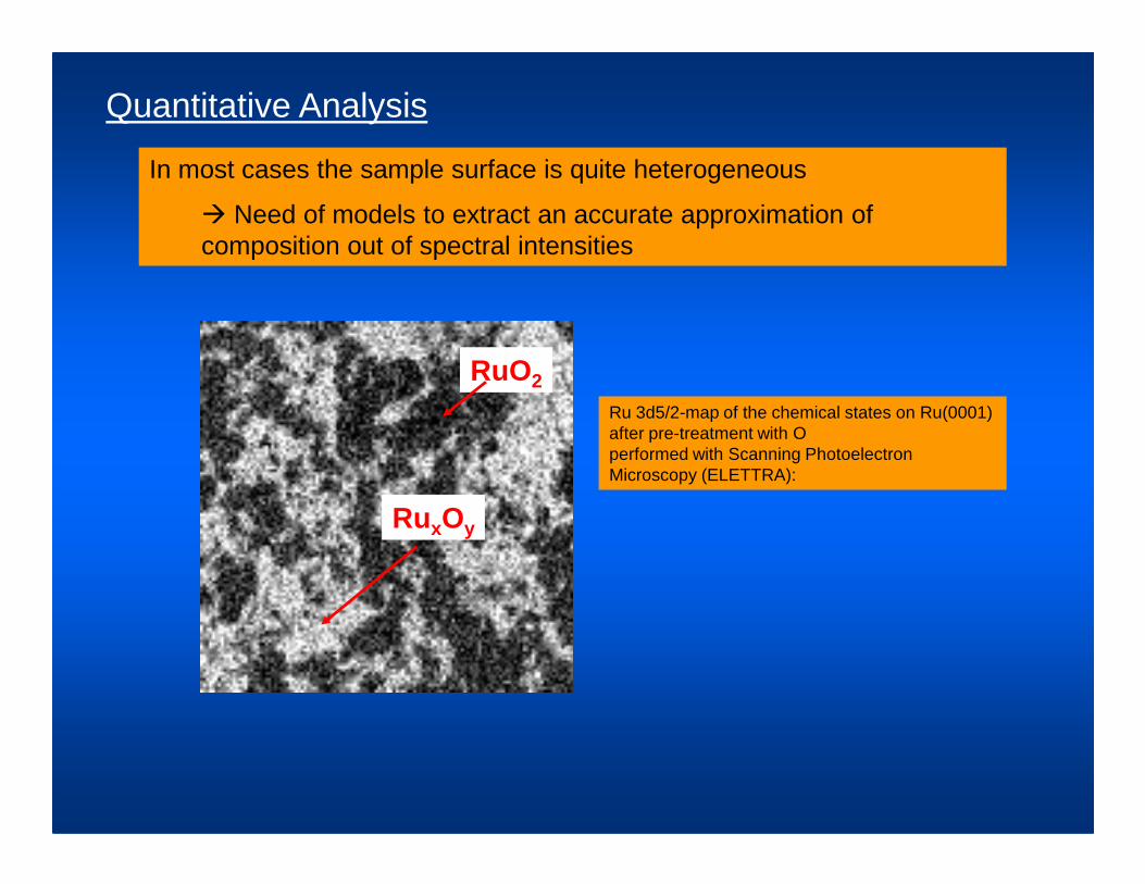
In most cases the sample surface is quite heterogeneous
� Need of models to extract an accurate approximation of composition out of spectral intensities
RuO2
Ru 3d5/2-map of the chemical states on Ru(0001) after pre-treatment with O
RuxOy
after pre-treatment with Operformed with Scanning Photoelectron Microscopy (ELETTRA):

Quantitative Analysis: Useful Examples
with the formulas above follows
a : „radius of A“
A. Heterogeneous mixture (e.g. alloy):
andaA: „radius of A“
���� Mol fraction
IA,B0: reference of
clean materialfollows

Quantitative Analysis: Useful Examples
B. Partial Coverage (e.g. adsorbat):
Contribution of B:
(attenuated by A) (direct)
For signals of A and ΘΘΘΘA: coverage
ΘΘΘΘ: angle between surface normal and emitted electron
For signals of A and B follows
ΘΘΘΘA: coverage of A on B
Which givesIA,B
0 : reference of clean material

Quantitative Analysis: Useful Examples
C. Thin layer of A on B (e.g. oxide):
Contribution of B:
Contribution of A:
���� Special case:
i.e.
Which gives
follows
General problem here: proper background substraction

Fundamental limit:
elastic and inelastic scattering of electrons in the gas phase
In situ XPS: obstaclesIn situ XPS: obstacles
30x10-21
25
20
15
10
Ioni
zatio
n cr
oss
sect
ion
(m2 )
in situEXAFSin situ
O2 exp. data from Schram et al. (1965) extrapolation of Schram's data
Technical issues: - Differential pumping to keep analyzer in high vacuum- Sample preparation and control in a flow reactor
5
0
Ioni
zatio
n cr
oss
sect
ion
(m
101
102
103
104
105
106
Electron kinetic energy (eV)
in situSEM
in situTEM
EXAFSin situXPS

• Photons enterthrough a window
• Electrons and a gas
In situ XPS: basic conceptIn situ XPS: basic concept
• Electrons and a gasjet escape throughan aperture tovacuum
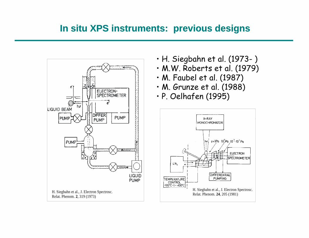
• H. Siegbahn et al. (1973- )• M.W. Roberts et al. (1979)• M. Faubel et al. (1987) • M. Grunze et al. (1988)• P. Oelhafen (1995)
In situ XPS instruments: previous designsIn situ XPS instruments: previous designs
H. Siegbahn et al., J. Electron Spectrosc. Relat. Phenom. , 319 (1973)2
H. Siegbahn et al., J. Electron Spectrosc. Relat. Phenom. , 205 (1981)24
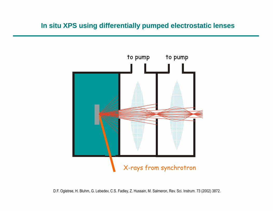
In situ XPS using differentially pumped electrostat ic lensesIn situ XPS using differentially pumped electrostat ic lenses
to pump to pump
D.F. Ogletree, H. Bluhm, G. Lebedev, C.S. Fadley, Z. Hussain, M. Salmeron, Rev. Sci. Instrum. 73 (2002) 3872.
X-rays from synchrotron

Gas phase composition can be measured by XPS.gas phase signal: 1 torr·mm ~ a few monolayers
CloseClose--up of sampleup of sample--first aperture regionfirst aperture region
hνp0
gas
z
de-1.0
0.5
0.0-2 -1 0 1 2
z [d]
p/p 0
z=2 mm
d=1 mm

In situ XPS systemIn situ XPS system
X-rays enter the cell at 55° incidence through an SiNx window (thickness ~ 1000 Å)
Analyzer input lens
Focal point
Hemisphercalelectronanalyzer(10-9p0)
mass spectrometerand additional
Experimental cellsupplied by gas lines (p0)
Focal point of analyzerinput lens
First differentialpumping stage (10-4p0)
Second differentialpumping stage (10-6p0)
Third differentialpumping stage (10-8p0)
mass spectrometerand additional pumping
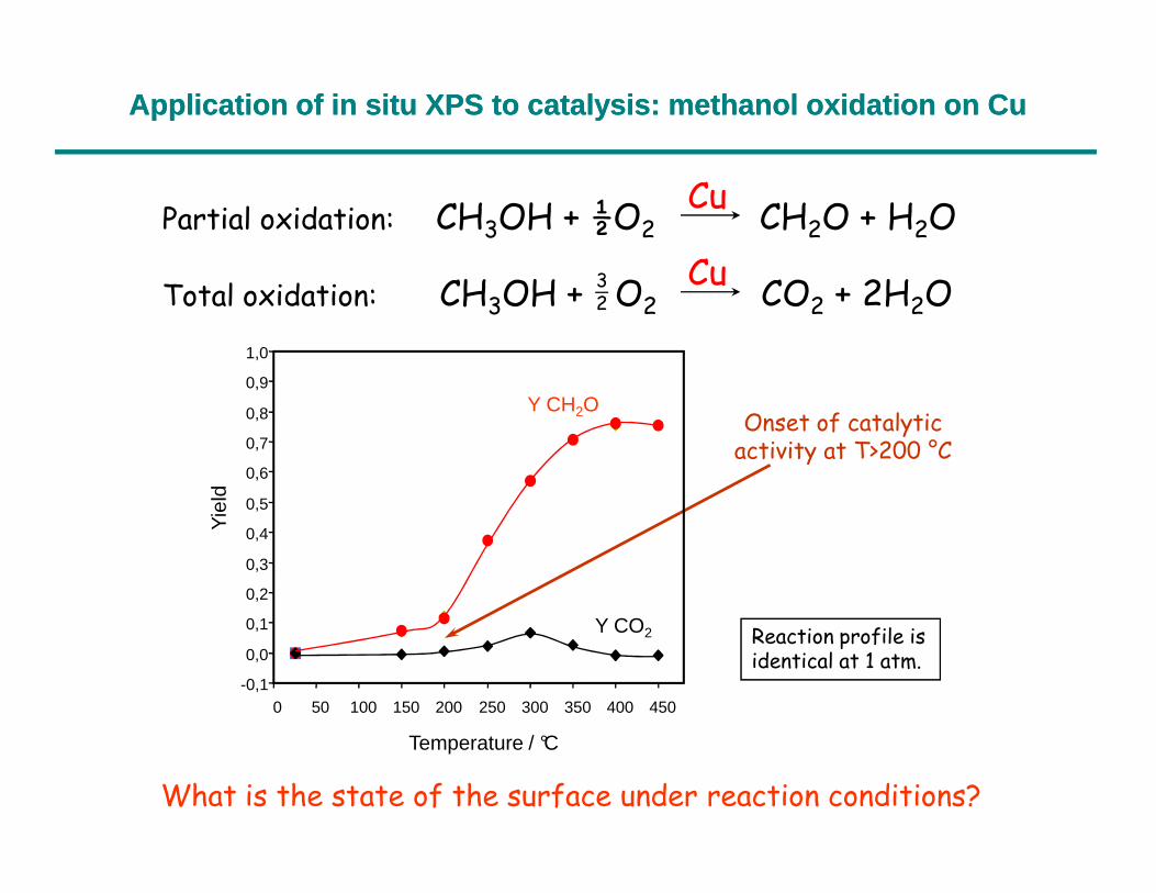
Partial oxidation: CH3OH + ½O2 CH2O + H2O
Total oxidation: CH3OH + O2 CO2 + 2H2O
Cu
Cu32
Application of in situ XPS to catalysis: methanol o xidation on CuApplication of in situ XPS to catalysis: methanol o xidation on Cu
Onset of catalyticactivity at T>200 °C0,7
0,8
0,9
1,0
Y CH2O
What is the state of the surface under reaction conditions?
Reaction profile isidentical at 1 atm.
activity at T>200 °C
-0,1
0,0
0,1
0,2
0,3
0,4
0,5
0,6
0,7
0 50 100 150 200 250 300 350 400 450
Temperature / °C
Yie
ld
Y CO2

CO + H O2 2
CH OH3
CH OH3
CH OH
CO+ H2
In situ NEXAFS
I.E. Wachs & R.J. Madix, Surf. Sci. 76, 531 (1978); A. F. Carley et al., Catal. Lett. 37, 79 (1996).UHV XPS
O-(a) + 2CH3OH(g) 2CH3O-(a) + H2O(g)
CH3O-(a) CH2O(g) + H+(a)
Partial oxidation of methanolPartial oxidation of methanol
CH O+ H2 2O
O+ O
CH OH3CH OH3
CH O+ H2 2
O2
Cu 0
Oxsurf
Oxbulk
Subox
Ovol
A. Knop-Gericke et al., Topics Catal. 15, 27 (2001).
In situ NEXAFS
Questions for in situ XPS: - Quantitative analysis of surface species- Carbon species on the surface- Depth-dependent analysis
CH3OH + O2 ~ 0.5 mbar
suboxide phase: - only present in situ
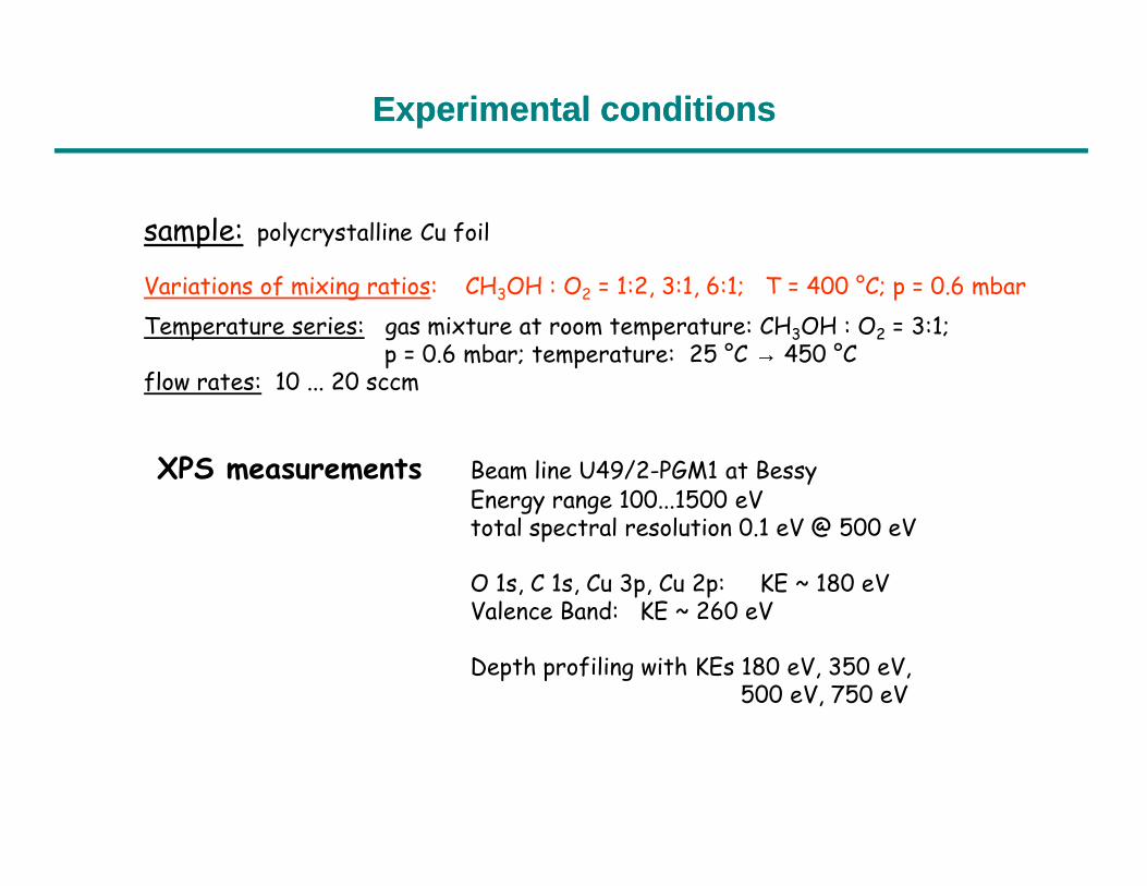
Experimental conditionsExperimental conditions
sample: polycrystalline Cu foil
Variations of mixing ratios: CH3OH : O2 = 1:2, 3:1, 6:1; T = 400 °C; p = 0.6 mbar
Temperature series: gas mixture at room temperature: CH3OH : O2 = 3:1; p = 0.6 mbar; temperature: 25 °C → 450 °C
flow rates: 10 ... 20 sccm
XPS measurements Beam line U49/2-PGM1 at BessyEnergy range 100...1500 eVtotal spectral resolution 0.1 eV @ 500 eV
O 1s, C 1s, Cu 3p, Cu 2p: KE ~ 180 eVValence Band: KE ~ 260 eV
Depth profiling with KEs 180 eV, 350 eV,500 eV, 750 eV

VB
∆ ~ 2 eV
160
140
120
100
Nor
mal
ized
cou
nt r
ate
(cps
/mA
)
CH
3OH
(g)CH
2O (
g)H
2O (
g)
CO
2(g
)
O2 (g) Cu2O
?
?
Methanol oxidation on Cu: O1s spectraMethanol oxidation on Cu: O1s spectra
400 °C, 0.5 torr
CH3OH:O2
O 1s
8 6 4 2 0 -2Binding energy (eV)
80
60
40
20
0
Nor
mal
ized
cou
nt r
ate
(cps
/mA
)
542 540 538 536 534 532 530 528 526
Binding energy (eV)
1:2
3:1
6:1
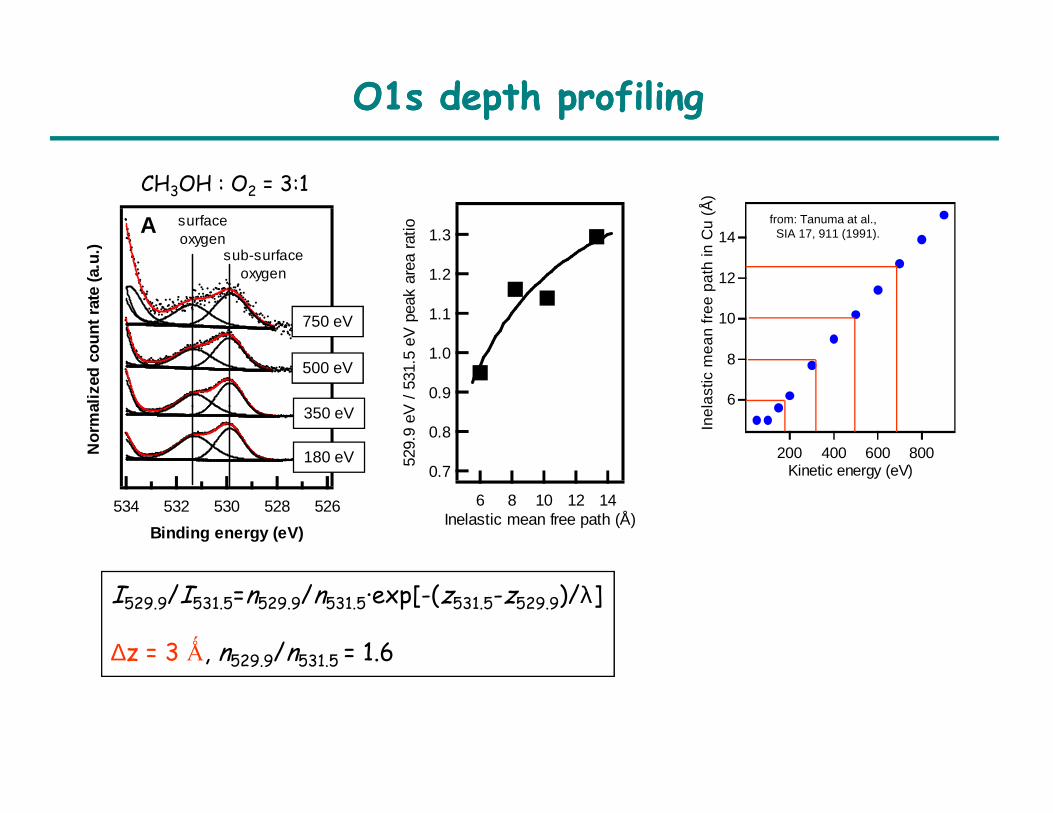
O1s depth profilingO1s depth profiling
1.3
1.2
1.1
1.0
0.952
9.9
eV /
531
.5 e
V p
eak
area
rat
io
14
12
10
8
6
Inel
astic
mea
n fr
ee p
ath
in C
u (Å
)
from: Tanuma at al., SIA 17, 911 (1991).
CH3OH : O2 = 3:1
Nor
mal
ized
cou
nt r
ate
(a.u
.) sub-surfaceoxygen
surfaceoxygen
A
350 eV
500 eV
750 eV
0.8
0.7
529.
9 eV
/ 5
31.5
eV
pea
k ar
ea r
atio
14121086Inelastic mean free path (Å)
I529.9/I531.5=n529.9/n531.5·exp[-(z531.5-z529.9)/λ]
∆z = 3 Ǻ, n529.9/n531.5 = 1.6
6
Inel
astic
mea
n fr
ee p
ath
in C
u (Å
)
800600400200Kinetic energy (eV)
Nor
mal
ized
cou
nt r
ate
(a.u
.)
534 532 530 528 526
Binding energy (eV)
180 eV
350 eV

Methanol oxidation on Cu: C1s spectraMethanol oxidation on Cu: C1s spectra
CO
2(g
)
CH
3OH
(g)
CH
2O (
g)
Camorph
C 1s160
140
120
100
Nor
mal
ized
cou
nt r
ate
(cps
/mA
)
CH
3OH
(g)CH
2O (
g)H
2O (
g)
CO
2(g
)
O2 (g) Cu2Osub-surface
oxygensurfaceoxygen
400 °C
CH3OH:O2
O 1s
292 288 284 280
Binding energy (eV)
80
60
40
20
0
Nor
mal
ized
cou
nt r
ate
(cps
/mA
)
542 540 538 536 534 532 530 528 526
Binding energy (eV)
1:2
3:1
6:1

Metastability of the SubMetastability of the Sub--Surface OxygenSurface Oxygen
CH
3OH
(g)
sub-surfaceoxygensurface
oxygen
H2O
(g)
CH
2O (
g)
CH3OH:O2=6:1
CH
3OH
(g)
sub-surfaceoxygensurface
oxygen
H2O
(g)
CH
2O (
g)
CH3OH:O2=6:1
536 534 532 530 528
Binding energy (eV)
CH3OH:O2=6:1
CH3OH only
difference
536 534 532 530 528
Binding energy (eV)
CH3OH:O2=6:1
CH3OH only
difference

Correlation of catalytic activity and surface speciesCorrelation of catalytic activity and surface species
CH2O yield vs sub-surface oxygen peak area
0.20
0.15
3:1
6:1
O p
artia
l pre
ssur
e (m
bar) mixing ratio series
(T = 400 °C)400 °C
400 °C temperature series(CH OH:O =3:1)
0.10
0.05
0.00
543210
normalized sub-surface oxygen peak area
1:2
CH
2O p
artia
l pre
ssur
e (m
bar)
250 °C
300 °C450 °C
150 °C
200 °C
temperature series(CH3OH:O2=3:1)
Open questions: What is the nature of the sub-surface oxygen species?What is its role in the catalytic reaction?
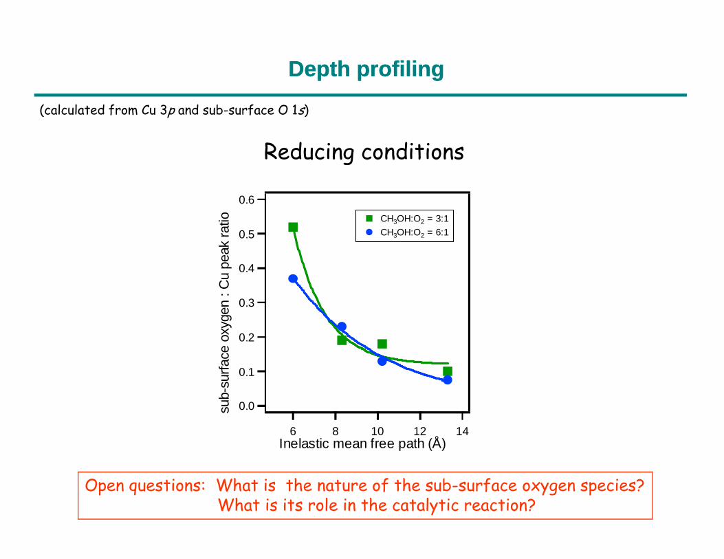
Depth profilingDepth profiling
0.6
0.5
0.4
sub-
surfa
ce o
xyge
n : C
u pe
ak ra
tio CH3OH:O2 = 3:1
CH3OH:O2 = 6:1
(calculated from Cu 3p and sub-surface O 1s)
Reducing conditions
0.3
0.2
0.1
0.0sub-
surfa
ce o
xyge
n : C
u pe
ak ra
tio
14121086Inelastic mean free path (Å)
Open questions: What is the nature of the sub-surface oxygen species?What is its role in the catalytic reaction?
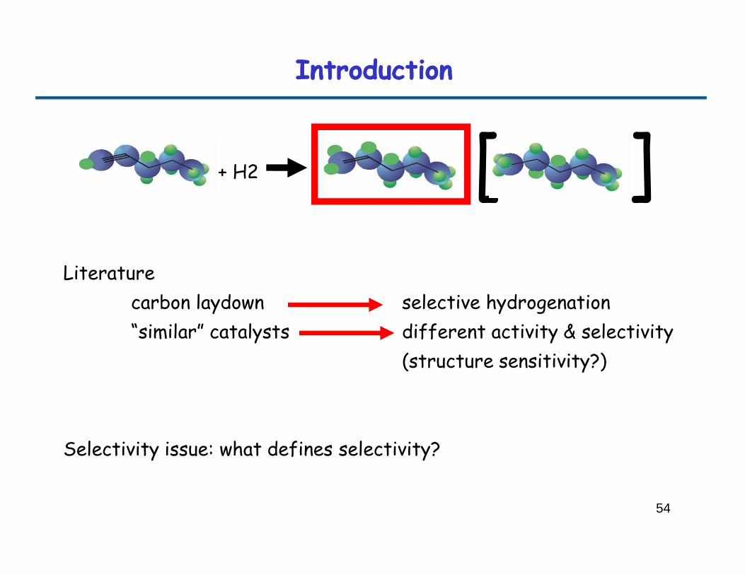
IntroductionIntroduction
Literature
[ ]+ H2
54
carbon laydown selective hydrogenation“similar” catalysts different activity & selectivity
(structure sensitivity?)
Selectivity issue: what defines selectivity?

InIn--situ XPS: situ XPS: Pd 3d (hPd 3d (hνννννννν: : 720 eV)720 eV)

InIn--situ XPS: situ XPS: Pd 3d depth profilingPd 3d depth profiling
Not only adsorbate-induced surface core level surface core level
shift !
But on-top location!
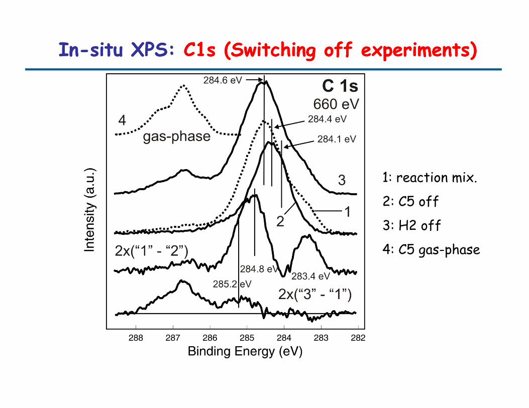
InIn--situ XPS: situ XPS: C1s (Switching off experiments)C1s (Switching off experiments)
1: reaction mix.
2: C5 off2: C5 off
3: H2 off
4: C5 gas-phase
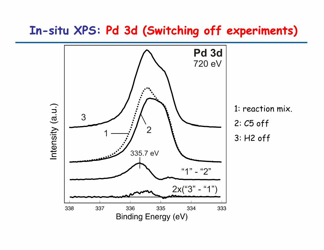
InIn--situ XPS: situ XPS: Pd 3d (Switching off experiments)Pd 3d (Switching off experiments)
1: reaction mix.
2: C5 off2: C5 off
3: H2 off
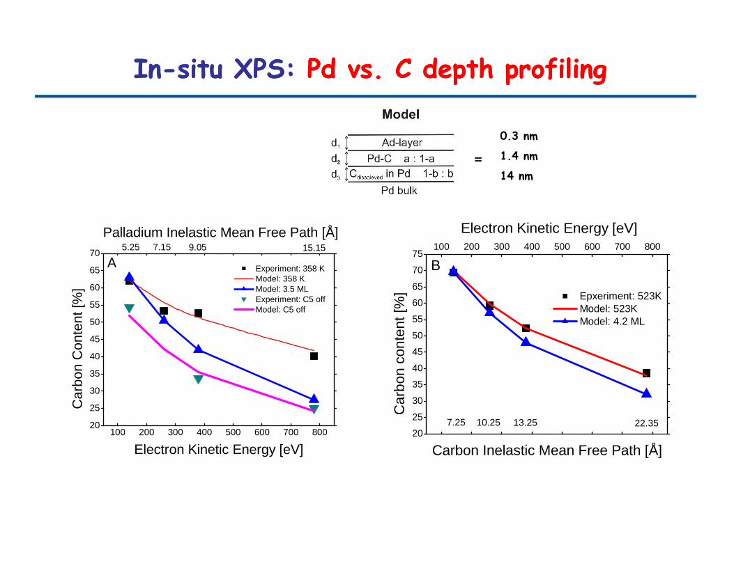
InIn--situ XPS: situ XPS: Pd vs. C depth profilingPd vs. C depth profiling
60
65
70A
Palladium Inelastic Mean Free Path [Å]
Experiment: 358 K Model: 358 K
5.25 7.15 9.05 15.15
65
70
75100 200 300 400 500 600 700 800
Electron Kinetic Energy [eV]
B
0.3 nm
1.4 nm
14 nm
100 200 300 400 500 600 700 80020
25
30
35
40
45
50
55
60
Car
bon
Con
tent
[%]
Electron Kinetic Energy [eV]
Model: 3.5 ML Experiment: C5 off Model: C5 off
20
25
30
35
40
45
50
55
60
65
22.3513.2510.25
Car
bon
cont
ent [
%]
Carbon Inelastic Mean Free Path [Å]
Epxeriment: 523K Model: 523K Model: 4.2 ML
7.25
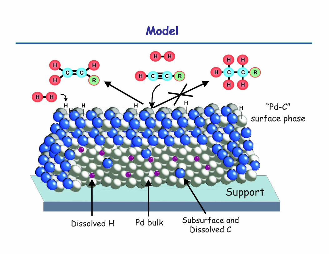
ModelModel

core statesatom specificquantitativecomplex final state effects chemical shift concept
Summary
chemical shift concept theoretically difficult accessiblecan be applied in the mbar rangesurface sensitivedepth profiling

1. W. Göpel, Chr. Ziegler: Struktur der Materie: Grundlagen, Mikroskopie undSpektroskopie , Teubner Verlagsgesellschaft, Stuttgart-Leipzig, 19912. M. Henzler, W. Göpel: Oberflächenphysik des Festkörpers , TeubnerVerlagsgesellschaft, Stuttgart-Leipzig, 19913. W. Göpel, Chr. Ziegler : Einführung in die Materialwissenschaften , TeubnerVerlagsgesellschaft, Stuttgart-Leipzig, 19964. D. Briggs, M. P. Seah: Practical Surface Analysis, Volume 1: Auger and X-R ayPhotoelectron Spectroscopy , 2. Auflage, John Wiley & Sons, Chichester, 19905. C. D. Wagner, W. M. Riggs, L. E. Davis, J. F. Moulder, G. E. Muilenberg: Handbookof X-Ray Photoelectron Spectroscopy , Physical Electronics Division, Perkin-ElmerCorporation, Eden Prairie, Minnesota, 19796. H. Lüth: Surfaces and Interfaces of Solid Materials , 3. Auflage, Springer Verlag,Berlin, 1995
Literature
Berlin, 19957. G. Ertl, J. Küppers: Low Energy Electrons and Surface Chemistry , VCHVerlagsgesellschaft, Weinheim, 19858. K. Siegbahn, C. Nording et al.: ESCA Applied to Free Molecules , North-Holland,Amsterdam, 19719. M. Cardona, L. Ley: Photoemission of Solids , Topics in Applied Physics, Band 26und 27, Springer Berlin, 197810. M. Grasserbauer, H. J. Dudek, M. F. Ebel: Angewandte Oberflächenanalyse mitSIMS, AES und XPS , Springer Berlin, 197911. D. Briggs and J. T. Grant: Surface Analysis by Auger and Photoelectron Spectroscopy , Surface Spectra and IM Publications 2003