photocatalytic oxidation for the removal of … oxidation for the removal of chlorpyrifos from...

Photocatalytic Oxidation for the Removal of

Chlorpyrifos from Aqueous Solution

A Major Qualifying Project Report

Submitted to the Faculty of

WORCESTER POLYTECHNIC INSTITUTE

In partial fulfillment of the requirement for the

Degree of Bachelor of Science

Submitted by:

Iliana Schulman

Dominique Throop

Project Advisors:

Professor Fred Hart, WPI

Professor John Bergendahl, WPI

Project Sponsor:

University of Nova Gorica

Submitted on:

December 21st, 2013

This report represents the work of two WPI project teams working in conjunction with one another. Consequently,

report JIB 1305 contains identical sections to report FLH AAEE.

ii

Abstract

Due to an increase in pesticide usage in agriculture worldwide, a need exists for the

development of an effective pollutant removal process for pesticides in agricultural run-off

water. It is advantageous for the treatment process to not require the addition of treatment

chemicals, which could potentially have harmful effects on the environment. An advanced

oxidation process (AOP) that utilizes titanium dioxide (TiO2) with exposure to ultraviolet light is

a possible treatment method for this application. Experiments were run using an immobilized

TiO2 catalyst in conjunction with a bench-scale batch reactor and a pilot-scale compound

parabolic collector (CPC) reactor to analyze the degradation of chlorpyrifos using UV-Visible

spectroscopy, HPLC, TOC, and LCMS. The fixed-film batch and CPC reactors yielded average

treatment efficiencies of 80% and 89.17%, respectively, after 4 hours, suggesting successful

degradation of chlorpyrifos using photocatalytic oxidation. The degradation of chlorpyrifos was

found to follow first order kinetics.

iii

Acknowledgements

We would like to take the time to thank all the individuals without whom this project would not

have been possible:

Professors John Bergendahl and Frederick Hart, our advisors, for their advice, guidance, and

organization while reviewing our report drafts and their overall help throughout the entirety of

this project. Without them, this project would not have been a success.

The faculty from the University of Nova Gorica (UNG), our sponsor, for the help and resources

provided to us throughout this project. All showed great hospitality for which we are extremely

grateful.

Thank you to all the individuals who took the time to meet with us during our time working on

this project to provide us with valuable advice and information:

Urška Lavrencic Stangar – Dean of the School of Environmental Sciences, UNG

Fernando Fresno – Research associate, Laboratory for Environmental Research (LRO),

UNG. Your mentorship allowed us to move forward through the various roadblocks in

this project.

Romina Žabar – PhD assistant, LRO, UNG. Our project would not have been possible

without your patient guidance.

Marko Kete – Young researcher, LRO, UNG. Had it not been for your efforts, our HPLC

analysis and TOC results would not have been possible.

Andraž Šuligoj – Young researcher, LRO, UNG. You aided us in starting this project and

without your direction we would have been at a loss.

Mitja Martelanc – PhD assistant, LRO, UNG. Without your aid in LCMS efforts the

intermediate compounds of chlorpyrifos may still be unknown.

Alex Margiott and Samuel Naseef – Your time and dedication in CAD allowed us to

accurately present our research. For this we are very grateful.

iv

Authorship

The chemical engineering students completing this WPI Major Qualifying Project are Iliana

Schulman and Dominique Throop. They worked in conjunction with Brendan Matheny and Jay

Ringenbach, both civil engineering students, to complete the following research. An MQP

report completed for civil engineering degree requirements can be found under the latter

mentioned names. Each member contributed different skills to make this project a success.

Below highlights some of the major responsibilities undertaken by each person:

Brendan Matheny is working toward completing his Civil Engineering degree with a

concentration in Environmental Engineering. Brendan spent a major part of the research

conducting work with Jay Ringenbach, performing CPC reactor experiments, and designing a

real-world application for a treatment system utilizing CPC reactors, while also compiling

Chapters 2 this report.

Jay Ringenbach is working toward completing his degree in Environmental Engineering

obtaining a commission in the United States Marine Corps. Jay spent a major part of the

research conducting work with Brendan Matheny, performing CPC reactor experiments, and

designing a real-world application for a treatment system utilizing CPC reactors, while also

compiling Chapters 3 this report.

Iliana Schulman is working toward completing her degree in Chemical Engineering. Iliana spent

a major part of the research conducting work with Dominique Throop, performing the fixed-

film batch reactor experiments to determine the degradation kinetics of chlorpyrifos while also

compiling Chapter 1 and the Appendices of this report.

Dominique Throop is working toward completing her degree in Chemical Engineering.

Dominique spent a major part of the research conducting work with Iliana Schulman,

performing the fixed-film batch reactor experiments to determine the degradation kinetics of

chlorpyrifos while also compiling Chapter 4 & 5 of this report.

v

Executive Summary

Background

Over the past decade, an increase of pesticide usage has been found in agriculture worldwide,

causing escalation in immunity among pests. Consequently, multiple pesticides are being used

in conjunction with one another to protect crops. Once applied, these compounds integrate

into runoff water, posing a substantial threat to any life form with which they come into

contact [EPA, 2012].

Remediation of pesticide-contaminated wastewater has begun to draw interest among the

scientific community. Since pesticides are nearly impossible to remove using traditional

biological approaches, heterogeneous photocatalysis using a semiconductor such as TiO2 has

received much attention as a sustainable application for wastewater treatment [Quiroz, 2011].

The following research explores photocatalytic oxidation in the presence of UV light in

conjunction with the use of TiO2 as a catalyst to degrade the organophosphate commonly

known as chlorpyrifos, an insecticide widely used in agriculture.

Experimental Methods

A bench-scale UV-photocatalytic batch reactor and a pilot-scale compound parabolic collector

(CPC) reactor, both using immobilized fixed-film coatings of titanium dioxide, were utilized to

conduct experiments with the aim of determining the degradation rate of chlorpyrifos in the

photocatalytic reaction. Experiments were carried out with starting concentrations of 2.0, 1.5,

1.0, and 0.5 ppm chlorpyrifos prepared in double deionized water. The fixed-film batch reactor

and CPC reactor were both run for four hours during each experiment to determine the

reaction kinetics of the TiO2/UV photocatalytic reaction.

Methods of Analysis

All samples taken from these experiments were analyzed through the use of high performance

liquid chromatography (HPLC) and total organic carbon (TOC). HPLC analysis of the

vi

photocatalytic reaction provided valuable data concerning the degradation of chlorpyrifos as

well as showing intermediate generation and consequent degradation. TOC analysis of the

photocatalytic reaction showed the degradation of the total carbon concentration over time.

Using the results gathered from these two analysis methods, further samples were selected for

liquid chromatography/mass spectrometry (LCMS) analysis. Specifically, samples displaying the

largest area for a potential intermediate found in the HPLC chromatograms were analyzed for

the identification of unknown intermediates and their chemical components.

Results

Chlorpyrifos was determined to follow a first order reaction rate, with the majority of

degradation occurring within the first hour of TiO2/UV treatment. The average treatment

efficiency after four experiments in the fixed-film batch reactor was calculated to be 80%. An

experimental treatment efficiency of approximately 89.17% for the first two hours of treatment

in the CPC reactors was calculated using data taken from HPLC. Potential intermediates were

proposed based off of data from LCMS analysis.

Conclusions

During experimentation, the majority of chlorpyrifos removal occurred as a result of adsorption

onto the catalyst surface prior to photocatalytic degradation. This can likely be attributed to the

fact that the catalyst film was cleaned using double deionized water under UV exposure for 30

minutes before each experiment. These conditions produce recombination sites that are

completely empty prior to experimentation, therefore not representative of actual operating

conditions.

TOC results showed degradation of the total carbon concentration over time, suggesting that

chlorpyrifos had degraded and formed intermediates that decomposed into gaseous CO2, which

then transferred from solution. LCMS results showed the generation of intermediates including

C9H11Cl3NO4P, C8H12Cl3O3PS, and C6H5NO2. Although chlorpyrifos oxon was determined to be

vii

slightly less toxic than chlorpyrifos, the relative toxicities of the remaining intermediates were

unable to be determined.

Recommendations

It is recommended that further testing be carried out on the fixed-film batch reactor and CPC

reactor with more frequent sampling and temperature testing. This would serve to aid in more

accurately identifying intermediates, which may be generated toward the end of the reaction.

Toxicity studies should be conducted for all intermediates. Furthermore, tracking temperature

changes over the course of a reaction could serve to highlight trends such as variability in

reaction rate. It is also recommended that a dip coating process be utilized when coating glass

slides with catalyst. This would ensure a uniform thickness of catalyst, as opposed to the

variability that can result from hand brushing. When attempting to determine actual

concentrations of samples being analyzed through HPLC, a dilution series from one large

quantity of reliable stock solution should be analyzed each time as well. In this manner it would

be possible to overcome variability that was inherent in HPLC over time. Lastly, the CPC reactor

being used should utilize construction techniques that allow for ease of operation. If the reactor

were easy to operate it would be a much simpler matter to replicate experimental conditions.

Aspects of the reactor design that should be changed include the use of threaded adapters as

opposed to push-on fittings, braided stainless steel tubing to avoid kinks that can reduce flow,

and an easily accessible filling port as well as a drainage valve.

viii

Table of Contents

Abstract ..................................................................................................................................................................... ii Acknowledgements ............................................................................................................................................. iii Authorship .............................................................................................................................................................. iv

Executive Summary.............................................................................................................................................. v

Background ......................................................................................................................................................... v

Experimental Methods ................................................................................................................................... v

Methods of Analysis ........................................................................................................................................ v

Results ................................................................................................................................................................. vi Conclusions ........................................................................................................................................................ vi Recommendations ......................................................................................................................................... vii

Table of Contents .............................................................................................................................................. viii 1.0 – Introduction ................................................................................................................................................. 1

2.0 – Background ................................................................................................................................................... 2

2.1 – Previous Pesticide Research in Slovenia ...................................................................................... 2

2.2 – Organic Pesticides ................................................................................................................................. 2

2.3 – Chlorpyrifos ............................................................................................................................................. 3

2.4 – Advanced Oxidation Processes ........................................................................................................ 5

2.5 – TiO2 Photocatalysis ............................................................................................................................... 6

2.6 – Photocatalysis Efficiency Variables ................................................................................................ 9

2.6.1 – Catalyst Composition ................................................................................................................... 9

2.6.2 – Catalyst Concentration ............................................................................................................. 11

2.6.3 – Pesticide Concentration ........................................................................................................... 12

2.6.4 – Wavelength ................................................................................................................................... 13

2.6.5 – Temperature ................................................................................................................................ 14

2.6.6 – UV Irradiation .............................................................................................................................. 14

2.7 – Reactor Parameters ........................................................................................................................... 15

2.7.1 – Slurries vs. Fixed-Film Reactors ........................................................................................... 15

2.7.2 – Fixed-Film Batch Reactor ........................................................................................................ 16

2.7.3 – Compound Parabolic Collector (CPC) Reactor ................................................................ 18

3.0 – Methodology.............................................................................................................................................. 21

3.1 – Chlorpyrifos Solution Preparation ............................................................................................... 21

3.2 – UV-Visible Light Spectroscopy ...................................................................................................... 22

3.3 – Calibration Curve ................................................................................................................................ 23

3.4 – Establishing Experimental Controls ............................................................................................ 24

3.5 – Small-Scale Slurry Reactor Experiments ................................................................................... 27

3.6 – Fixed-Film Batch Reactor ................................................................................................................ 29

3.6.1 – Fixed-Film Batch Reactor Preparation .............................................................................. 30

3.6.2 – Flushing the Fixed-Film Batch Reactor .............................................................................. 32

3.6.3 – Draining the Fixed-Film Batch Reactor ............................................................................. 33

3.6.4 – Operating the Fixed-Film Batch Reactor ........................................................................... 33

3.7 – UV Photocatalytic CPC Reactor ..................................................................................................... 34

3.7.1 – CPC Catalyst Preparation ........................................................................................................ 34

3.7.2 – CPC Reactor Preparation ......................................................................................................... 36

ix

3.7.3 – CPC Reactor Operation ............................................................................................................. 36

3.8 – Methods of Analysis ........................................................................................................................... 38

3.8.1 – HPLC Analysis Process ............................................................................................................. 38

3.8.2 – TOC Analysis Method ................................................................................................................ 39

3.8.3 – LCMS Analysis Method ............................................................................................................. 40

4.0 – Results & Discussion .............................................................................................................................. 41

4.1 – Analysis of UV-Visible Light Spectroscopy ............................................................................... 41

4.2 – HPLC Calibration Curve.................................................................................................................... 43

4.3 – Experimentation Using the Slurry Batch Reactor .................................................................. 44

4.4 – Glass Slide Coating ............................................................................................................................. 46

4.5 – Fixed-Film Batch Reactor HPLC Results .................................................................................... 48

4.6 – CPC Reactor HPLC Results .............................................................................................................. 52

4.7 – TOC Results ........................................................................................................................................... 54

4.8 – LCMS Results ........................................................................................................................................ 56

5.0 – Conclusions & Recommendations .................................................................................................... 64

5.1 – Glass Coating ........................................................................................................................................ 65

5.2 – HPLC and TOC Analysis .................................................................................................................... 65

5.3 – LCMS Analysis ...................................................................................................................................... 66

5.4 – Slurry Reactor ...................................................................................................................................... 66

5.5 – Fixed-Film Batch Reactor ................................................................................................................ 67

5.6 – CPC Reactor........................................................................................................................................... 68

5.7 – Possible Application .......................................................................................................................... 69

5.8 – Future Research .................................................................................................................................. 69

References ............................................................................................................................................................ 70

Appendix A – Equipment ................................................................................................................................ 72

Appendix B – Chlorpyrifos in Acetonitrile Solution ............................................................................. 80

Appendix C – Batch & CPC Reactor HPLC Results Run with Water ................................................ 93

Appendix D – Batch Reactor and CPC Reactor TOC Results .............................................................. 99

Appendix E – Preparing 1F Solution ......................................................................................................... 104

Appendix F – Determination of Treatment Efficiency ....................................................................... 105

Appendix G – LCMS Chromatograms ........................................................................................................ 106

Appendix H – High Performance Liquid Chromatography (HPLC) .............................................. 107

Appendix I – Slide Coating Procedure ...................................................................................................... 109

x

Table of Figures

Figure 2.1: Chlorpyrifos molecular structure [Sigma-Aldrich]. 3

Figure 2.2: Current Advanced Oxidation Technologies [Fraunhofer IGB]. 5

Figure 2.3: Band gap energy of titanium dioxide compared to other photocatalysts [Fresno, 2013].

6

Figure 2.4: Electron hole pair production [Fresno, 2013]. 7

Figure 2.5: P25 vs. PC500 TiO2. 9

Figure 2.6: Reaction Rate vs. Catalyst Mass [Herrmann, 2010]. 11

Figure 2.7: Reaction Rate vs. Pollutant Concentration [Herrmann, 2010]. 12

Figure 2.8: Reaction Rate vs. Wavelength [Herrmann, 2010]. 13

Figure 2.9: Solar radiation spectrum [Haenke, 2010]. 13

Figure 2.10: Reaction Rate vs. Temperature [Herrmann, 2010]. 14

Figure 2.11: Reaction Rate vs. Irradiance [Herrmann, 2010]. 14

Figure 2.12: Fixed-Film batch reactor. 16

Figure 2.13: 3-D schematic of fixed-film batch reactor. 17

Figure 2.14: CPC reactors in Almeria, Spain [Compound Parabolic Collector (CPC) Photoreactors, 2013].

18

Figure 2.15: Front view of CPC reactor. 19

Figure 2.16: Side view of CPC reactor. 20

Figure 3.1: UV darkness box closed (top left), UV darkness box opened (top right), inside of UV darkness box with UV light source above stir plate (bottom).

25

Figure 3.2: Fixed-Film batch reactor. 29

Figure 3.3: 2D Schematic of fixed-film batch reactor. 30

Figure 3.4: a) Hexagonal glass slide holder b) loaded batch reactor chamber c) metal crossbars securing reactor.

31

Figure 3.5: 2D schematic of hexagonal slide holder being loaded into the glass batch reactor chamber, sealing the chamber, and loading it inside the metal reactor.

32

Figure 3.6: CPC reactor. 34

Figure 3.7: (From left to right) round steel holders, commercial grade TiO2 catalyst embedded in porous paper, wrapped steel holders, holders being inserted into the chamber of the CPC reactor.

35

Figure 4.1: UV/Vis Spectrophotometer screen shot. 41

Figure 4.2: 2 ppm chlorpyrifos solution with red lines denoting wavelengths of 200 and 230 nm.

42

Figure 4.3: Calibration curve for solution of chlorpyrifos at concentrations of 2.0, 1.0, 0.5, and 0 ppm.

43

Figure 4.4: Concentration over time of control solution used in slurry reactor experiments.

44

Figure 4.5: Unintegratable chlorpyrifos peaks (increasing time from top to bottom). 45

Figure 4.6: Chlorpyrifos degradation in UV-photocatalytic fixed-film batch reactor with an initial concentration of 2.29 ppm.

50

Figure 4.7: Graph depicting the slope of the line = α for batch reactor with starting concentration of 2.29 ppm.

51

Figure 4.8: Natural log of efficiency versus time to find the value of the rate constant, k.

52

Figure 4.9: Degradation of chlorpyrifos in CPC reactor. 53

Figure 4.10: Generation of intermediate during chlorpyrifos degradation in CPC reactor.

53

Figure 4.11: TOC over time from UV-photocatalytic fixed-film batch reactor. 54

xi

Figure 4.12: Theoretical TOC of chlorpyrifos samples. 55

Figure 4.13: Theoretical TOC (red squares) versus actual TOC (blue diamonds). 55

Figure 4.14: Mass spectrogram of 2 ppm slurry reactor at t=42. 57

Figure 4.15: Mass spectrogram of 0.5 ppm CPC reactor at t= 285. 57

Figure 4.16: Elution times 9.316-9.433 from Figure 4.15. 57

Figure 4.17: Possible pathways of organophosphates in aqueous TiO2 suspension [Konstantinou, 2002].

58

Figure 4.18: Persistence of C5H2Cl3NO over time. 60

Figure 4.19 (repeated): Generation of intermediate during chlorpyrifos degradation in CPC reactor.

61

Figure 4.20: Intermediate generation. 61

Figure 4.21: Chlorpyrifos oxon. 62

xii

Table of Tables

Table 2.1: Advantages and disadvantages of immobilized fixed-film and small-scale slurry reactors.

15

Table 3.1: Dilution needed for each concentration of solution. 23

Table 3.2: Times at which both control and TiO2 samples were taken out of the beaker, centrifugation began, and were filtered into HPLC vials in parallel.

26

Table 3.3: Small-scale slurry reactor timetable. 28

Table 4.1: Surface area, weight, and final thickness for glass slides used in the photocatalytic batch reactor.

47

Table 4.2: HPLC results and concentrations. 49

Table 4.3: Calculations and values needed to find reaction order, α, and reaction constant, k.

50

Table 4.4: Samples from each experiment analyzed by LCMS identifiable by the type of reactor, the starting concentration, and the time at which the sample was taken. Samples 5 and 12, highlighted, produced useable results.

56

Table 4.5 Possible intermediates generated during chlorpyrifos degradation. 59

1

1.0 – Introduction

As the population of the planet continues to increase, a larger supply of water is required for

society’s needs, including drinking and agricultural use. Over the past decade, organic pesticide

usage in agriculture worldwide has been on the rise, resulting in an increase of pollutants found

in various water sources. The type of pollutants found in water sources largely depends upon

the local industries. Urban and agricultural wastewaters often contain pesticides, herbicides,

fungicides, insecticides (organic compounds), and PCBs as pollutants [Oblak, 2013] and these

pollutants can end up in water sources.

Over the past decade, organic pesticide use in agriculture worldwide has been increasing [MSDS

– 45395, 2013]. Pesticides are defined as artificially synthesized substances that are used to

fight pests and improve agricultural production [Miguel, 2007]. In recent years, the variety and

concentration of pesticides used in the Mediterranean region has drastically increased due to a

developing immunity to pesticides [Ballesteros, 2009]. Slovenia in particular has been severely

affected by chemical pollution from organic pesticides and fungicides used in vineyards

[Ambrožic, 2008]. The presence of these hazardous substances must be eliminated to sustain

reusable water for the general population.

Due to an increased threat of pollution, remediation of pesticide-contaminated wastewaters

has drawn interest among the scientific community. There exists a need for the development of

an effective pollutant removal process that does not require the addition of treatment

chemicals, which could potentially have other harmful effects on the environment. Since

traditional biological treatment is not a feasible option due to the effect of pesticides on

microorganisms, biological treatment is generally impractical. However, advanced oxidation

processes (AOPs) allow for the breakdown of bio recalcitrant compounds into intermediates

and in some cases produce even complete mineralization if properly executed. Titanium dioxide

irradiated with ultraviolet light (TiO2/UV) is an advanced oxidation process that has not yet

been fully explored for the purpose of water and wastewater treatment. The use of TiO2/UV

treatment was evaluated in this project specifically for the removal of chlorpyrifos from water.

2

2.0 – Background

2.1 – Previous Pesticide Research in Slovenia

From 2001-2009, the Agricultural Institute of Slovenia (AIS) collected data regarding Plant

Protection Products (PPP). PPPs are generally considered to be any chemical, (pesticides,

herbicides, fungicides, plants growth regulators or otherwise) that is used to kill, repel, or

control pest, influence the life cycle of plants, or destroy weeds. Eight locations around the

country were monitored to better understand how to develop environmentally friendly PPPs

that must reach the standards set by the Slovenian national government. The AIS study found

that 28.6% of the grape samples from Slovenian vineyards exceeded the set level of PPPs

[Česnik, 2011].

2.2 – Organic Pesticides

Organic pesticides in water are frequently resistant to traditional biological treatment

[Ballesteros, 2009]. The complex molecular structure of organic pesticides often inhibits

biological treatment processes due to the generation of dangerous, highly toxic intermediates.

Although difficult to remove through a single biological process, conversion of such pollutants

into biodegradable intermediates, or even their mineralization products, can be accomplished

through photocatalytic pretreatment, resulting in the biodegradability of organic pesticide

pollutants [Quiroz, 2011].

3

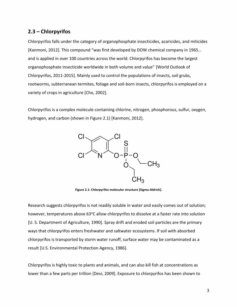
2.3 – Chlorpyrifos

Chlorpyrifos falls under the category of organophosphate insecticides, acaricides, and miticides

[Kanmoni, 2012]. This compound “was first developed by DOW chemical company in 1965…

and is applied in over 100 countries across the world. Chlorpyrifos has become the largest

organophosphate insecticide worldwide in both volume and value” [World Outlook of

Chlorpyrifos, 2011-2015]. Mainly used to control the populations of insects, soil grubs,

rootworms, subterranean termites, foliage and soil-born insects, chlorpyrifos is employed on a

variety of crops in agriculture [Cho, 2002].

Chlorpyrifos is a complex molecule containing chlorine, nitrogen, phosphorous, sulfur, oxygen,

hydrogen, and carbon (shown in Figure 2.1) [Kanmoni, 2012].

Figure 2.1: Chlorpyrifos molecular structure [Sigma-Aldrich].

Research suggests chlorpyrifos is not readily soluble in water and easily comes out of solution;

however, temperatures above 63oC allow chlorpyrifos to dissolve at a faster rate into solution

[U. S. Department of Agriculture, 1990]. Spray drift and eroded soil particles are the primary

ways that chlorpyrifos enters freshwater and saltwater ecosystems. If soil with absorbed

chlorpyrifos is transported by storm water runoff, surface water may be contaminated as a

result [U.S. Environmental Protection Agency, 1986].

Chlorpyrifos is highly toxic to plants and animals, and can also kill fish at concentrations as

lower than a few parts per trillion [Devi, 2009]. Exposure to chlorpyrifos has been shown to

4

produce a variety of nerve disorders in humans. It is readily absorbed into the bloodstream

through the gastrointestinal tract if ingested, through the lungs if inhaled, or through the skin if

there is skin exposure [Chemical fact sheet for chlorpyrifos, 1984]. Absorption through the skin

may result in systemic intoxication, or poisoning of the bodily system [Chlorpyrifos, n. d.].

Symptoms of chlorpyrifos poisoning include headaches, nausea, muscle convulsions, birth

defects, and in very rare cases death [Devi, 2009]. This is due to the inhibition of the

cholinesterase enzyme, which is required for proper nerve functioning [Cho, 2002]. In addition

to causing inhibition of cholinesterase, acute exposure to chlorpyrifos may also cause skin

irritation. Since chlorpyrifos is absorbed through the skin, contact with the pesticide should be

avoided [Chemical fact sheet for chlorpyrifos, 1984]. Repeated exposures to chlorpyrifos can,

without warning, causes heightened susceptibility to doses of any cholinesterase inhibitor

[MSDS – 45395, 2013].

The Pesticide Incident Monitoring System reported three hundred and nineteen human

exposure incidents from 1970 through 1981, most resulting from inhalation and skin exposure.

Three human deaths during this study were caused by chlorpyrifos or chlorpyrifos combined

with other active ingredients. Persons with respiratory ailments, recent exposures to

cholinesterase inhibitors, cholinesterase impairment, or liver malfunction are at increased risk

from exposure to chlorpyrifos [Guidance for re-registration of pesticides containing chlorpyrifos

as the active ingredient, 1984].

5

2.4 – Advanced Oxidation Processes

Advanced oxidation processes (AOPs) break down organic compounds such as alcohols,

aldehydes, carboxylic acids, amines, and specifically insecticides and herbicides into carbon

dioxide and water with trace mineral acids. AOPs are useful in wastewater treatment due to the

complete mineralization of bio-recalcitrant pollutants such as chlorpyrifos under the right

conditions. AOPs are also an inexpensive alternative to more expensive chemical mineralization

processes [Quiroz, 2011]. Figure 2.2 outlines many current technologies that utilize AOPs.

Figure 2.2: Current Advanced Oxidation Technologies [Fraunhofer IGB].

The production of free hydroxyl radicals (OH•) is a fundamental step in the advanced oxidation

process due to their non-selective attack of organic pollutants [Zapata, 2009]. Hydroxyl radicals

oxidize organic contaminants, making them extremely useful for wastewater treatment.

Hydroxyl radicals mineralize many organic molecules while yielding CO2 and inorganic ions as

byproducts when driven to completion [Zapata, 2009]. The versatility of AOPs makes it easy to

produce hydroxyl radicals by allowing specific treatment requirements to be met [Zapata,

2009].

6

2.5 – TiO2 Photocatalysis

This research presents the AOP known as photocatalysis, which uses titanium dioxide (TiO2) as a

catalyst in the presence of ultraviolet radiation. Photocatalysis is defined as a change in the rate

of a chemical reaction under ultraviolet, visible, or infrared radiation in the presence of a

photocatalyst by absorbing light to produce a chemical transformation of the reactants

[Braslavsky, 2007]. The excited state of the photocatalyst repeatedly interacts with the

reactants to form reaction intermediates while regenerating itself after each cycle of

interactions [Braslavsky, 2007].

Using TiO2 as a semiconductor for photocatalytic reactions is a promising new process for

wastewater treatment. Titanium dioxide is a material with numerous applications, recently

because of its capacity to be photo activated by solar light [Coronado & Hernandez-Alonso,

2013]. The inert biological and chemical nature of TiO2, as well as a resistance to chemical and

photo corrosion, is a major advantage to using TiO2 as a photo catalyst.

Figure 2.3: Band gap energy of titanium dioxide compared to other photocatalysts [Fresno, 2013].

Titanium dioxide has the capability to treat a wide range of organic pesticides with the

appropriate radiation conditions. Photocatalysis uses TiO2 in conjunction with UV radiation of

photon wavelength less than 400 nm, since the band-gap energy of TiO2 is 3.2 eV (Figure 2.3).

This AOP is considered one of the most efficient processes for lowering the concentration of

7

pesticides in wastewater [Quiroz, 2011]. The reaction that occurs is an oxidation reaction that

requires TiO2 as a catalyst to produce CO2, H2O, and intermediates.

When atoms come together to form molecules, their atomic orbitals are shared to yield two

molecular orbitals: bonding (low energy) and antibonding (high energy). These new orbitals

attempt to minimize the energy of the system through valence electrons by filling only the

bonding orbitals. With an increasing number of atoms, the energy gap between two adjacent

molecular orbitals decreases. Therefore, in a solid with a theoretically infinite number of atoms,

energy bands are formed rather than discrete orbitals. The highest occupied band in a solid is

called the valence band, while the lowest unoccupied band is referred to as the conduction

band. The gap of forbidden energy states between the valence and conduction bands of a solid

is called the band gap. When the band gap energy (3.2 eV in the case of TiO2) is exceeded by

absorption of a photon, electrons in the valence band move across the band gap into the

conduction band to create electron-hole pairs, which then initiate the photocatalytic reaction.

The hole left behind in the valence band then oxidizes the organic contaminant while the

excited electrons reduce oxygen in the solution. Hydroxyl radicals are generated as

intermediates of this photocatalytic reaction [Chong, 2010]. Figure 2.4 below shows the process

by which TiO2 and UV light create electron hole-pairs on the catalyst surface.

Figure 2.4: Electron hole pair production [Fresno, 2013].

8

Recombination is one of the main disadvantages of photocatalysis due to the waste of energy in

the system. Occurring in the absence of electron acceptors/donors, recombination limits the

quantum yield. Prevention of electron-hole pair recombination is therefore crucial to the

photocatalytic process in order to increase efficiency of the process. Addition of external

electron acceptors increases the rate of degradation, hydroxyl radical concentration, and

oxidation rate of intermediates by preventing recombination. Electron acceptors, such as H2O2

or O3, play an important role in the production of hydroxyl radicals [Chong, 2010]. TiO2 has

shown enhanced activity compared to other catalysts under solar radiation due to its high

surface area and high capacity to adsorb water and hydroxyl groups on the catalyst surface

[Devi, 2009].

9

2.6 – Photocatalysis Efficiency Variables

Optimizing the efficiency of TiO2 photocatalysis requires many factors to be taken into account

when considered for wastewater treatment. The semiconductor used in this study, TiO2, plays a

key role in the photocatalytic process, but many other variables can also affect the oxidation

process. Among them are: catalyst composition, catalyst concentration, pesticide

concentration, light wavelength, temperature, and UV intensity.

2.6.1 – Catalyst Composition

The two types of TiO2 catalyst used in this study are P25 and PC500 (Figure 2.5). The differences

in photocatalytic activity between these two types of catalyst can most likely be traced back to

the difference of surface area and density of hydroxyl groups on the catalyst surface. These

factors affect the adsorption behavior of the pollutant and recombination rate of electron-hole

pairs. The particle size of TiO2 is an important factor to consider since it directly affects the

efficiency of the catalyst through surface area.

Figure 2.5: P25 vs. PC500 TiO2.

10

P25 has a specific surface area of 50 m2g-1. PC500, on the other hand, has a specific surface area

of 287m2g-1. PC500 is 100% anatase versus P25 being 75% anatase and 25% rutile by mass.

While PC500 titanium dioxide has a much larger surface area than P25, the opposite is true of

the crystal size. P25 has a crystal size of 21nm when compared to a 5-10 nm crystal size for

PC500 [Chong, 2010].

Through past research conducted by Urh Černigoj at UNG, it was determined that the most

effective mixture for research utilizing a TiO2 small-scale slurry reactor is a 1:1 ratio of

Millennium’s PC500 and Degussa’s P25 TiO2. This ratio creates the best possible “balance

between surface area and crystallinity… to obtain the highest photo activity” [Černigoj, 2006].

11

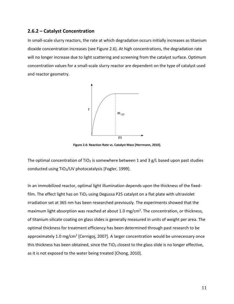
2.6.2 – Catalyst Concentration

In small-scale slurry reactors, the rate at which degradation occurs initially increases as titanium

dioxide concentration increases (see Figure 2.6). At high concentrations, the degradation rate

will no longer increase due to light scattering and screening from the catalyst surface. Optimum

concentration values for a small-scale slurry reactor are dependent on the type of catalyst used

and reactor geometry.

Figure 2.6: Reaction Rate vs. Catalyst Mass [Herrmann, 2010].

The optimal concentration of TiO2 is somewhere between 1 and 3 g/L based upon past studies

conducted using TiO2/UV photocatalysis [Fogler, 1999].

In an immobilized reactor, optimal light illumination depends upon the thickness of the fixed-

film. The effect light has on TiO2 using Degussa P25 catalyst on a flat plate with ultraviolet

irradiation set at 365 nm has been researched previously. The experiments showed that the

maximum light absorption was reached at about 1.0 mg/cm2. The concentration, or thickness,

of titanium silicate coating on glass slides is generally measured in units of weight per area. The

optimal thickness for treatment efficiency has been determined through past research to be

approximately 1.0 mg/cm2 [Cernigoj, 2007]. A larger concentration would be unnecessary once

this thickness has been obtained, since the TiO2 closest to the glass slide is no longer effective,

as it is not exposed to the water being treated [Chong, 2010].

12

2.6.3 – Pesticide Concentration

The concentration of pollutant being treated in a photocatalytic process can significantly affect

the rate of reaction. When the duration of radiation and catalyst concentration remain fixed,

the concentration of hydroxyl radicals and O2• on the catalyst surface appears to remain

constant. Therefore, not enough hydroxyl radicals are generated to participate in degradation

at higher concentrations of pesticide, meaning that either UV intensity or catalyst

concentration is the limiting factor [Chong, 2010].

Figure 2.7 below shows the relationship between reaction rate and pollutant concentration for

any given reaction. Higher concentrations of pollutant lead to an increased reaction rate. As

shown, a plateau is reached once a certain concentration is present. Since all adsorption sites

are in use, additional pollutant cannot react with the catalyst surface until recombination sites

are free.

Figure 2.7: Reaction Rate vs. Pollutant Concentration [Herrmann, 2010].

13

2.6.4 – Wavelength

The wavelength and intensity of light radiation is a key parameter in affecting reaction rate. If

the wavelength of the light source provides energy lower than the energy threshold, E0, the

desired reaction will not occur (Figure 2.8). In the case of TiO2 it is known that a wavelength

lower than 400 nm is required for a photocatalytic reaction to commence.

Figure 2.8: Reaction Rate vs. Wavelength [Herrmann, 2010].

While the < 400nm wavelength falls in the UV radiation range, only 3-5% of the solar spectrum

is used in the oxidation process. In other words, only 4% of sunlight will be used in a given

reaction with a titanium dioxide catalyst (Figure 2.9).

Figure 2.9: Solar radiation spectrum [Haenke, 2010].

14

2.6.5 – Temperature

At temperatures above 80°C, the lower adsorption of pollutant leads to decreased activity and

slower reaction rates. On the other hand, lower temperatures favor adsorption, including that

of reaction products, which may become inhibitors. Therefore, a temperature of about 20-50°C

is recommended for this particular oxidation process, as shown in Figure 2.10 [Herrmann,

2010].

Figure 2.10: Reaction Rate vs. Temperature [Herrmann, 2010].

2.6.6 – UV Irradiation

As the intensity of UV irradiation increases, the reaction rate for the degradation of the

targeted contaminants increases (Figure 2.11). Once the activation energy (3.2 eV) required to

excite electrons into the next valence band of TiO2 is achieved, the rate of degradation will no

longer increase with increased UV intensity. This implies that, should the intensity required to

excite electrons be exceeded, no further recombination sites will be created, causing energy to

be wasted.

Figure 2.11: Reaction Rate vs. Irradiance [Herrmann, 2010].

15

2.7 – Reactor Parameters

Optimizing the efficiency of a photoreactor requires many design components be taken into

account when considering heterogeneous photocatalysis for wastewater treatment. A

photoreactor that accounts for variables, such as solar radiation, must be designed to efficiently

degrade pollutants, specifically from vineyard runoff. Two primary reactors commonly used in

solar photocatalytic processes are fixed-film batch reactors and immobilized fixed-film pilot

scale compound parabolic collector (CPC) reactors, which are essential to testing various

circumstances at the pilot scale level.

2.7.1 – Slurries vs. Fixed-Film Reactors

Pilot-scale reactors may be designed to utilize either small-scale slurry or immobilized fixed-film

catalysts. The use of TiO2 in suspended form is more efficient than in immobilized form. As

shown in Table 2.1, each type of reactor utilizes distinct operating parameters that both come

with their own set of advantages and disadvantages [Chong, 2010].

Table 2.2: Advantages and disadvantages of immobilized fixed-film and small-scale slurry reactors.

Slurry Advantages Slurry Disadvantages Fixed-film

Advantages

Fixed-film Disadvantages

Greater possible TiO2

Concentrations, allowing

for increased treatment

efficiency

TiO2 recovery must occur

before the release of

effluent

No TiO2 recovery

required before discharge

High TiO2 concentrations

are not possible, meaning

lower treatment

efficiency possibilities

Faster reaction rate High TiO2 concentration

results in opaque

solutions, which can block

UV irradiation

Film is self-cleaning in the

presence of UV light

Slower reaction rate

Greater surface area

exposure

Surface area limitations

16

2.7.2 – Fixed-Film Batch Reactor

The fixed-film batch reactor used in this study forces chlorpyrifos solution into contact with

immobilized TiO2. To achieve an accurate reaction, the catalyst surface must be uniformly

coated. This bench-scale study must be conducted to provide information regarding the

reaction kinetics before further research on reactor design can begin [Černigoj, 2006]. Figure

2.12 details a technical drawing of the process used. A 3-D model showing the specific reactor

shown can be found in Figure 2.13. The pesticide infused water is added at the mixer labeled

“sampling”, pumped through Stream 1 into the pump, through Stream 2 into the reactor

containing the immobilized catalyst and UV light source where it will be treated, and back to

the mixer via Stream 3.

Figure 2.12: Fixed-Film batch reactor.

17

Figure 2.13: 3-D schematic of fixed-film batch reactor.

Reactor Shell

< Main Chamber with UV Source

Pump

Sampling Beaker

18

2.7.3 – Compound Parabolic Collector (CPC) Reactor

A pilot system in Almeria, Spain has provided valuable information on the reactor parameters

that must be considered for this study [Compound Parabolic Collector (CPC) Photoreactors,

2013]. Figure 2.14 shows the pilot system in Almeria, Spain.

Figure 2.14: CPC reactors [Compound Parabolic Collector (CPC) Photoreactors, 2013].

CPC reactors utilize fixed-film cylinders wrapped in commercial TiO2 that are placed throughout

the reactor tubes to expose the pesticide-contaminated water to the greatest surface area

possible. The diameter of piping in a CPC photoreactor is critical to both photon absorption and

the hydraulics within a reactor. Steady flow ensures that a uniform residence time can be

obtained, allowing for equal treatment of all water passing through a given reactor. Reactors

with diameters that are small in relation to their flow rate yield higher velocities and can

produce turbulent flow. As a result, efficient treatment can be difficult to carry out. Ideally, a

more laminar flow rate aids in increasing treatment efficiencies. Refer to Figure 2.15 & 2.16 for

a 2D diagram of the reactor used for experimentation at UNG.

19

Figure 2.15: Front view of CPC reactor.

Figure 2.15 above shows the front view schematic for the CPC reactor used at UNG. As shown in

the diagram, a pump circulates 5.5 L of solution through one reactor tube over the duration of

an experiment. All other tubes are not used during the reaction due to an inefficient use of

chemicals used to make solution. The dimensions of the reactor are approximately 1.5 m in

length by 2 m in height.

20

Figure 2.16: Side view of CPC reactor.

Figure 2.16 above shows the side view schematic for the CPC reactor used at UNG. As shown in

the diagram, a pump circulates 5.5 L of solution through one reactor tube (third from the

bottom as highlighted in Figure 2.16)) over the duration of an experiment. All other tubes were

not used during the reaction due to an inefficient use of chemicals required to make solution.

The UV light hood pictured only covers a small section of the reactor since only one tube was

used when performing experiments. The dimensions of the reactor are approximately 1.5 m in

width by 1.3 m in height.

21

3.0 – Methodology

This chapter details experimental procedures and analysis. The procedures presented refer only

to experiments conducted with solutions of chlorpyrifos suspended in double deionized water,

and do not reflect the initial stage of the project, which was conducted using chlorpyrifos

suspended in a solution of 10% acetonitrile and 90% double-deionized water (refer to Appendix

B). All equipment mentioned in this section is clearly documented with pictures, descriptions

and model information that can be found in Appendix A.

3.1 – Chlorpyrifos Solution Preparation

Preparing a standardized solution to use in each experiment was critical to ensuring accurate,

repeatable results. The following procedure was used to prepare chlorpyrifos solutions at 2

ppm in water:

1. Approximately 900 mL of double deionized water was added to a 1000 mL beaker.

2. A magnetic stir bar was added to the beaker, which was placed on a stirring plate with a

heating function. The water was heated to approximately 63 °C.

3. 2 mg of chlorpyrifos were weighed and added to the beaker containing heated water.

4. Parafilm was placed over the beaker to prevent any possible pesticide volatilization or

evaporation of water.

5. The solution was allowed to mix for approximately an hour after this point, or until

completely homogenous (i.e. no white flecks or phase separation could be seen in the

colorless, transparent solution).

6. Once the pesticide was completely dissolved, the solution was transferred to a 1000 mL

volumetric flask and the final volume adjusted to 1L with double deionized water.

7. The 2 ppm solution was allowed to cool to room temperature and then used to prepare

all necessary dilutions.

22

3.2 – UV-Visible Light Spectroscopy

To analyze the results of each experiment using High Performance Liquid Chromatography

(HPLC), it was necessary to determine the wavelength at which the clearest signals from

samples containing chlorpyrifos were detected. To accomplish this, a UV-visible light

spectrophotometer (UV-Vis) was employed to register the adsorption spectrum of chlorpyrifos

with wavelengths of 200, 230, and 290 nm considered for analysis.

Samples of chlorpyrifos solution and double deionized water were prepared and placed in

quartz cuvettes, which could be used for UV-Vis analysis to determine the wavelengths

associated with chlorpyrifos in the following manner:

1. Using a quartz cuvette, a blank consisting of double deionized water was analyzed by

the spectrophotometer in order to zero the machine.

2. Again, using a quartz cuvette, 2 ppm chlorpyrifos solution was analyzed by UV-Vis.

Since each compound absorbs light at a certain wavelength, similar to a fingerprint, it is

possible to associate a chemical with a specific absorption wavelength. Using double deionized

water as a blank served to ensure that no peaks were detected due to water. In this manner the

remaining peaks could be assumed to result from chlorpyrifos. The three wavelengths tested

could then be clearly evaluated and the one that provided the strongest signal for chlorpyrifos

would be chosen.

23

3.3 – Calibration Curve

A dilution series was prepared for HPLC testing to create a calibration curve. Solutions of 2.0,

1.5, 1.0, and 0.5 ppm chlorpyrifos were prepared in triplicate using double deionized water to

ensure accuracy. This was accomplished by utilizing Equation 2 to find the volume of the initial

solution to be added to double deionized water to dilute the solution to the desired lower

concentration (C2) as shown in Table 3.1.

𝐶1𝑉1 = 𝐶2𝑉2 [Equation 2]

Where C1 = Concentration of the initial solution

V1 = Necessary volume of the initial solution

C2 = Desired concentration

V2 = Desired volume of solution.

Table 3.1: Dilution needed for each concentration of solution.

C1 (ppm) V1 (mL) C2 (ppm) V2 (mL)

2.0 10.0 2.0 10.0

2.0 7.5 1.5 10.0

2.0 5.0 1.0 10.0

2.0 2.5 0.5 10.0

These four concentrations were used to create a calibration curve for chlorpyrifos in double

deionized water. Using the same reagent bottle of 2 ppm solution, dilutions of 1.5, 1.0, and 0.5

ppm were made. Three HPLC vials of each were filled and analyzed to create a reliable

calibration curve of concentration versus area. The area under the peak at the elution time of

chlorpyrifos could then be divided by the slope of the curve to determine concentration of

samples taken throughout each experiment.

24

3.4 – Establishing Experimental Controls

There are two processes within each experiment that may cause a decrease in the

concentration of chlorpyrifos in solution. The first is adsorption onto the catalyst surface and

the second is photocatalytic oxidation. As a way to distinguish between the adsorption of

chlorpyrifos onto the surface of the TiO2 catalyst and the reaction of chlorpyrifos and UV

radiation with the TiO2 catalyst, the beginning of each experiment was run in the dark.

By taking samples of chlorpyrifos solution containing suspended titanium dioxide catalyst in the

absence of UV light over time, it was possible to determine when the concentration of

chlorpyrifos was no longer decreasing. Once the time needed to reach this plateau had passed,

meaning the catalyst surface had been saturated with chlorpyrifos, the UV light source for the

experiment could be turned on and all degradation of chlorpyrifos after that time could be

assumed to be a result of photocatalytic oxidation.

To determine the time required for adsorption, two experiments were run in parallel: one

solution of 2 ppm chlorpyrifos containing suspended TiO2 and one control solution of 2 ppm

chlorpyrifos without TiO2. This was performed to ensure that no outside variables were

contributing to the decrease in concentration of chlorpyrifos, such as volatilization.

The total time required for complete adsorption onto the catalyst surface was determined by

carrying out the following procedure:

1. Two 50 mL samples of 2 ppm chlorpyrifos were prepared.

2. One 25 mg sample of P25 TiO2 (see Figure 3.4) was prepared and stored in an Eppendorf

flip-cap tube.

3. Both samples were placed in separate 100 mL beakers and a stir bar was added to each

beaker.

4. These beakers were placed on separate stir plates inside a darkness box (See Figure 3.1)

and covered in aluminum foil to ensure no light exposure.

25

5. One beaker was labeled as the control and the other was labeled as TiO2. The 25 mg

sample of titanium powder was added to the TiO2 beaker. Immediately after it was

mixed into the liquid, a 2 mL sample from each beaker was taken using a 5 mL syringe

and injected into Eppendorf flip-cap tubes. These tubes were labeled “C” for control and

“T” for titanium. (For example, T=0 min was the first sample taken. The remaining times

used can be found in Table 3.2.)

6. One minute after the samples were taken, both samples were placed into the centrifuge

and run for 4 minutes at 13.4 thousand rpm. (For example, T=1 min was when sample

T=0 was centrifuged.)

7. As soon as the centrifuge finished, the solution inside each Eppendorf vial was drawn

into a 5 mL syringe. This was done using a needle attachment on the syringe to be sure

not to disturb the pellet of TiO2 that had formed at the bottom of the vial. Likewise, the

Figure 3.1: UV darkness box closed (top left), UV darkness box opened (top right), inside of UV darkness box with UV light source above stir plate (bottom).

26

control sample was extracted in a similar manner. (For example, T=7 min was when

sample T=0 was filtered into an HPLC vial.)

8. The control sample was then injected directly into an HPLC vial labeled with the time the

sample was taken from the beaker, the concentration, and that it was the control.

9. A 0.45 micron filter was placed on the end of the syringe containing the TiO2 sample and

was filtered into a similarly labeled HPLC vial stating that it contained TiO2.

Table 3.2: Times at which both control and TiO2 samples were taken out of the beaker,

centrifugation began, and were filtered into HPLC vials in parallel.

Sample Taken (min) Centrifuged (min) Filtered (min)

1 0 1 5

2 7 8 12

3 14 15 19

4 21 22 26

5 28 29 33

6 35 36 40

Once the required time for complete adsorption had been obtained, all further experiments

utilized the known adsorption time. This allowed the reactors to cycle for the determined time

to ensure complete adsorption before activating a UV light source.

27

3.5 – Small-Scale Slurry Reactor Experiments

By turning the UV light source on after complete adsorption was achieved, it was possible to

distinguish between the decrease in concentration due to adsorption and the decrease in

concentration due to oxidation. Since the TiO2 slurry reacts with chlorpyrifos in a manner

similar to fixed-film TiO2, an initial rate could be approximated and used to estimate the time

required for the longer experiments with batch and compound parabolic collector (CPC) fixed-

film reactors. This experiment was essentially a continuation of the experiment used to

determine pesticide adsorption time as discussed above in Chapter 3.4. The initial laboratory

setup remained the same, as did the procedure until the previously determined time required

for complete adsorption had been reached. This time was found to be T = -7 minutes, as the UV

lamps needed time to warm up before conducting the experiment.

The following procedure used both a control sample containing chlorpyrifos in water and a

sample of chlorpyrifos in water with the addition of TiO2:

1. At T=-7 min, a 2 mL sample was taken from each beaker with a 5 mL syringe and

injected into labeled Eppendorf flip-cap tubes.

2. The beakers were covered with aluminum foil and the UV light source was switched on,

allowing the UV light to warm up without affecting the samples.

3. Steps 7-10 of Chapter 3.4 were repeated for all samples taken as shown in Table 3.2.

28

Table 3.3 below shows the times at which both control and experimental runs were taken from

the small-scale slurry reactor, centrifugation began, and filtration into HPLC vials occurred.

Table 3.3: Small-scale slurry reactor timetable.

Sample UV Status Taken (min) Centrifuged (min) Filtered (min)

1 UV with Tinfoil Covering -7 -6 -2

2 UV source 0 1 5

3 UV source 7 8 12

4 UV source 14 15 19





29

3.6 – Fixed-Film Batch Reactor

The fixed-film batch reactor pictured in Figure 3.2 was used to determine the degradation

reaction kinetics of chlorpyrifos in water at initial concentrations of 2.0, 1.5, 1.0, and 0.5 ppm.

The reactor consists of a polished aluminum housing which has UV lamps mounted at equal

intervals around the interior. The reactor itself is a two-piece glass vessel containing six glass

slides coated with catalyst, which is housed between the UV lamps. A 2D schematic of process

flow can be seen in Figure 3.3.

Figure 3.2: Fixed-Film batch reactor.

30

Figure 3.3: 2D schematic of fixed-film batch reactor.

3.6.1 – Fixed-Film Batch Reactor Preparation

The fixed-film batch reactor was prepared as follows:

1. Glass slides #5-12 were selected based on the mass of titanium silicate per cm2 of

surface area value being closest to 1.0 mg/cm2.

2. The top of the glass reactor was removed, as was the top of the plastic holder (female

adapter), to allow the slides to be loaded into every other slot in the cylindrical holder

as shown in Figure 3.4.a.

3. Teflon tape was wrapped around the end of the slides and the holder itself to secure

them.

4. The top of the holder was then replaced for additional physical support.

31

5. The holder was inserted into the glass chamber horizontally to avoid dropping the slides

to the bottom.

6. The top of the glass reactor was reattached and wrapped with parafilm in order to

prevent leakage as seen in Figure 3.4.b.

7. The reactor was carefully lowered into the metal reactor shell and secured with zip ties,

utilizing the metal crossbars as shown in Figure 3.4.c. The reactor loading process is

diagrammed in Figure 3.5.

8. The inlet and outlet were then connected to the pump using threaded plastic adapters.

Figure 3.4: a) Hexagonal glass slide holder b) loaded batch reactor chamber c) metal crossbars securing reactor.

32

Figure 3.5: 2D schematic of hexagonal slide holder being loaded into the glass batch reactor chamber, sealing the chamber,

and loading it inside the metal reactor.

3.6.2 – Flushing the Fixed-Film Batch Reactor

Once the reactor had been prepared, approximately 1.7 L of double deionized water was

funneled into the sampling container until full. The positive displacement pump was set at a

flow rate of 700.7 mL/min, a rotation of 156 rpm, and switched on. As soon as the sampling

beaker began to drain, double deionized water was added to the sampling beaker at a rate

approximately equal to the flow rate of the pump. Once the main chamber of the reactor was

full and the water began to pour back into the sampling beaker, water addition ceased, the UV

lights were switched on, and the system was allowed to run for a minimum of 30 minutes. This

ensured that any previous contaminants on the slides or in the chamber were removed.

33

3.6.3 – Draining the Fixed-Film Batch Reactor

1. The pump was switched off and the outlet tube was placed into a waste container. The

pump was then switched back on.

2. Once the sampling container was drained, the pump was stopped.

3. The inlet tube was removed from the sampling container and placed into the waste

beaker.

4. The direction of the pump was reversed and the pump was run until the system was

completely drained.

3.6.4 – Operating the Fixed-Film Batch Reactor

The process for loading the reactor with chlorpyrifos solution was similar to the process

described for flushing the reactor. The solution of desired concentration was funneled into the

sampling container. The glass slides previously loaded were used for all experiments, allowing

the reactor chamber to remain untouched. Once the main chamber was full and solution began

to pour back into sampling container, the system was allowed to run for 30 minutes in the dark

to accommodate the predetermined adsorption time. A sample of the solution being loaded

was taken for TOC and HPLC analysis using a 25 mL glass pipette connected to a Peleus ball and

injected into a 30 mL TOC vial. After the 30-minute adsorption time elapsed, UV lights were

switched on, an oxygen bubbler was placed into the sampling container, and the oxygen tank

valve was opened to a pressure between 0.5-0.7 bars. Samples were taken at 0, 5, 10, 20, 30,

60, 120, 180, and 240 minutes. The system was emptied as described above and flushed with

double deionized water after each experiment.

34

3.7 – UV Photocatalytic CPC Reactor

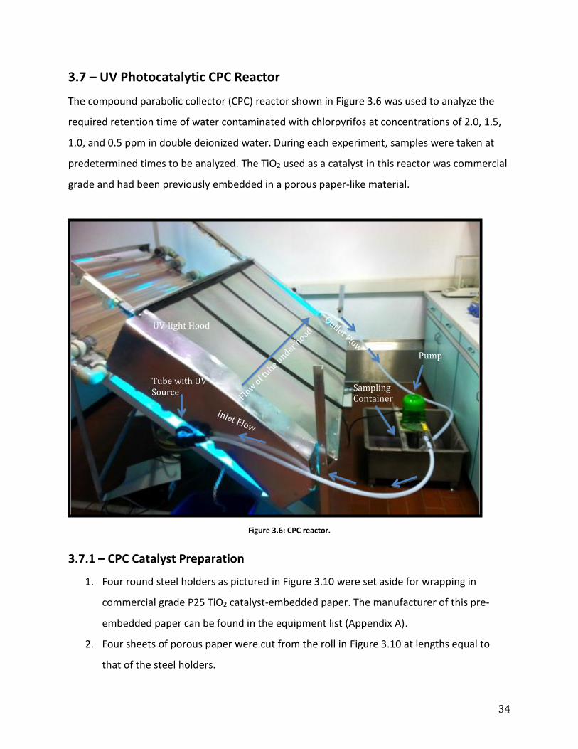
The compound parabolic collector (CPC) reactor shown in Figure 3.6 was used to analyze the

required retention time of water contaminated with chlorpyrifos at concentrations of 2.0, 1.5,

1.0, and 0.5 ppm in double deionized water. During each experiment, samples were taken at

predetermined times to be analyzed. The TiO2 used as a catalyst in this reactor was commercial

grade and had been previously embedded in a porous paper-like material.

Figure 3.6: CPC reactor.

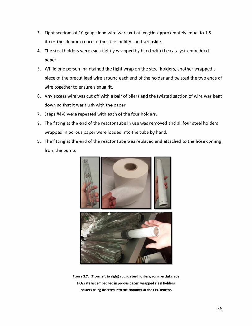
3.7.1 – CPC Catalyst Preparation

1. Four round steel holders as pictured in Figure 3.10 were set aside for wrapping in

commercial grade P25 TiO2 catalyst-embedded paper. The manufacturer of this pre-

embedded paper can be found in the equipment list (Appendix A).

2. Four sheets of porous paper were cut from the roll in Figure 3.10 at lengths equal to

that of the steel holders.

UV-light Hood

Pump

Sampling Container

Tube with UV Source

35

3. Eight sections of 10 gauge lead wire were cut at lengths approximately equal to 1.5

times the circumference of the steel holders and set aside.

4. The steel holders were each tightly wrapped by hand with the catalyst-embedded

paper.

5. While one person maintained the tight wrap on the steel holders, another wrapped a

piece of the precut lead wire around each end of the holder and twisted the two ends of

wire together to ensure a snug fit.

6. Any excess wire was cut off with a pair of pliers and the twisted section of wire was bent

down so that it was flush with the paper.

7. Steps #4-6 were repeated with each of the four holders.

8. The fitting at the end of the reactor tube in use was removed and all four steel holders

wrapped in porous paper were loaded into the tube by hand.

9. The fitting at the end of the reactor tube was replaced and attached to the hose coming

from the pump.

Figure 3.7: (From left to right) round steel holders, commercial grade

TiO2 catalyst embedded in porous paper, wrapped steel holders,

holders being inserted into the chamber of the CPC reactor.

36

3.7.2 – CPC Reactor Preparation

1. The volume of the CPC reactor is approximately 5.5 L, meaning that 5.5 L of the desired

sample needed to be prepared prior to each experiment.

2. With the pump valve closed, the sample solution was poured into a 2 L dish beneath

the pump until the container was filled and the pump was submerged.

3. A 25 mL sample was taken from this dish to serve as a sample for time T=-30 min. This

was accomplished using a 25 mL glass pipette connected to a Peleus ball.

4. The sample was then injected into a 30 mL TOC vial.

5. The pump was started and one person slowly opened the valve halfway while another

poured the remainder of the sample into the 2 L dish.

6. Once the solution was flowing continuously through the reactor, the valve was opened

completely and the half hour of adsorption time in the dark began.

3.7.3 – CPC Reactor Operation

1. After the adsorption time was complete, a sample at time T=0 min was taken to

determine how much chlorpyrifos had been adsorbed.

2. Immediately following, the UV lights were switched on and time recorded (using a

stopwatch).

3. Samples were taken in the manner described above at various time intervals.

4. After 300 minutes the UV light source and the pump were turned off.

5. The effluent line from the pump was removed from the reactor tube and placed in a

waste container.

6. The pump was turned on and allowed to drain the contents of the 2 L dish into a waste

container.

7. The pump was then turned off and the waste container was placed below the reactor

tube.

37

8. The cap on the reactor tube was removed, thus allowing the waste to drain. Since the

reactor is a few degrees off horizontal, draining this portion solely with the aid of

gravity was possible.

9. 2 mL samples were taken from each of the TOC vials and placed into HPLC vials using a

Pasteur pipette.

10. All vials were labeled appropriately and stored until the correct analysis equipment was

available for use.

38

3.8 – Methods of Analysis

Several different methods and instruments were used to analyze the data collected from the

reactors. The HPLC analysis allowed for degradation curves and intermediate generation curves

to be analyzed, the TOC analysis provided data for the creation of curves depicting the removal

of total organic carbon from solution, and the LCMS detailed peaks used to determine chemical

compositions needed to establish the identity of intermediate molecules.

3.8.1 – HPLC Analysis Process

3.8.1.a Reaction Kinetics

The reaction rate (r) at a known concentration may be determined from experimental results.

The reaction order is determined by graphing the natural log of the negative change in

concentration over change in time (−ln(−𝑑𝐶𝑎

𝑑𝑡)) versus the natural log of concentration (ln(𝐶𝑎))

and determining the slope of the line, α (see Equation 3). For the following experiments,

chlorpyrifos was the sole reactant, referred to as species A in the following equations. Equation

3 represents the generalized rate law.

−𝑟𝐴 = 𝑘𝐴𝐶𝐴𝛼𝐶𝐵

𝛽 [Equation 3]

Where 𝑟𝐴 = reaction rate,

𝑘𝐴 = rate constant

𝐶𝐴 = chlorpyrifos concentration,

𝐶𝐵 = concentration of species B

α = reaction order of species A

β = reaction order of species B

The rate law exists to describe the relationship of these variables at specific concentrations

[Folger, 2006].

39

Based on experimental data as well as previous research [Kanmoni, 2012], the reaction order

for the degradation of chlorpyrifos could be determined. The following equation represents a

first order reaction.

−𝑟𝐴 = 𝑘𝐴𝐶𝐴 [Equation 4]

Where 𝑘is in units of 𝑚𝑖𝑛−1.

3.8.1.b Calculations

Below is the process used to find the reaction order (α) and rate constant (k) for a given

concentration of chlorpyrifos in a UV-photocatalytic fixed-film reactor:

1. The changes in concentration and time from sample to sample were calculated using

Cfinal – Cinitial = C and Tfinal-Tinitial = T, respectively.

2. The natural log of concentration/time was then graphed against the natural log of

concentration corresponding to this change. For example, from 20 to 30 minutes would

have a t of 10 minutes and a C of C30min – C20min. The quotient of these values would

then be graphed against the natural log of C30min.

3. The slope of this graph gave the reaction order (α), referred to in Equation 3.

4. The specific reaction rate, also commonly referred to as the rate constant, k, can be

found through Equation 5, which also relies on the graph generated in step 3.

𝐿𝑁(𝑘𝐴) = 𝑦𝑖𝑛𝑡𝑒𝑟𝑐𝑒𝑝𝑡 [Equation 5]

5. The integral method may also be used for first order reactions, where the rate constant

can be obtained by plotting a graph of the negative natural log of final concentration

divided by initial concentration (−ln (𝐶𝑎

𝐶𝑎𝑜)) versus time. The slope of the line generated

is equal to the k value.

3.8.2 – TOC Analysis Method

Given the molecular formula of chlorpyrifos, C9H11Cl3NO3PS, and the known concentration of

solution being prepared, it was possible to determine the theoretical total organic carbon (TOC)

contained in a sample of a given volume and concentration. This value could then be used in

comparison to the results produced by the TOC analyzer to determine the difference between

40

actual and theoretical carbon content. In this manner, it was possible to ensure that the

machine was functioning properly.

Since any intermediate formed through the degradation of chlorpyrifos will contain carbon, the

TOC will remain of significant value until complete mineralization is achieved. This is due to the

fact that as CO2 is generated, it will immediately volatilize and leave solution; effectively

reducing the total carbon content of the sample.

By testing 2.0, 1.5, 1.0, and 0.5 ppm chlorpyrifos samples, a graph of chlorpyrifos concentration

versus carbon concentration could be generated. This served as a calibration curve and aided in

the analysis of chlorpyrifos mineralization.

3.8.3 – LCMS Analysis Method

Liquid chromatography/mass spectrometry (LCMS) was used to determine the composition of

several intermediates formed during the degradation process of chlorpyrifos. Using HPLC

results, samples from each experiment were taken at the highest peak of every intermediate

that appeared and analyzed by LCMS using the same column used for HPLC analysis. Elution

times that corresponded to peaks in both HPLC analysis and LCMS were used to determine

areas of focus. Once the necessary peaks were determined, the mass to charge ratio (m/z) for

each was used to identify possible compounds.

41

4.0 – Results & Discussion

Data presented in this chapter represent a portion of the research completed for this project.

Additional data and analysis containing all graphs and calculations relevant to this project can

be found in Appendices C & D. High Performance Liquid Chromatography (HPLC), Total Organic

Carbon (TOC), and Liquid Chromatography/Mass Spectrometry (LCMS) were used to analyze

photocatalytic oxidation reactions involving immobilized TiO2 in both bench-scale fixed-film

batch reactor and pilot scale compound parabolic collector (CPC) reactor. The degradation rate

of chlorpyrifos and its reaction kinetics provide the information necessary to design a full-scale

reactor. TOC analysis was used to determine the extent of mineralization. Similarly, LCMS

analysis identified intermediate compounds that could be studied for toxicity, aiding in the

determination of appropriate treatment levels.

4.1 – Analysis of UV-Visible Light Spectroscopy

UV-Visible light spectroscopy (UV-Vis) was used to determine the appropriate wavelength to

analyze a sample of 2 ppm chlorpyrifos solution with HPLC. The software configuration can be

seen in Figure 4.1. The HPLC analyzes each sample at wavelengths of 200, 230, and 290. As can

be seen in Figure 4.2, peaks appear on UV-Vis at all three wavelengths used for HPLC analysis.

Since the clearest, most defined wavelength occurred at 200 nm, this was the wavelength used

to analyze all HPLC results.

Figure 4.1: UV/Vis Spectrophotometer screen shot.

42

UV-Vis was also used to verify that the 0.45 micron filter used for the slurry reactor

experiments (Chapter 3.5) did not interfere with the solution analysis. Injecting a sample of

chlorpyrifos through the filter into a quartz cuvette and analyzing it determined that

chlorpyrifos did not have an affinity for the filter material surface and remained in solvent.

Analyzing one sample of filtered chlorpyrifos solution and one of unfiltered chlorpyrifos

solution side by side showed that the graphs were identical, meaning the filter had no effect on

the composition of chlorpyrifos in solution.

Figure 4.2: 2 ppm chlorpyrifos solution with red lines

denoting wavelengths of 200 and 230 nm.

43

4.2 – HPLC Calibration Curve

The calibration curve shown in Figure 4.3 represents samples of chlorpyrifos at concentrations

of 2.0, 1.0, 0.5, and 0 ppm (double deionized water). Analysis of 1.5 ppm samples resulted in

unreliable data that was dismissed for calibration purposes.

Figure 4.3: Calibration curve for solution of chlorpyrifos at concentrations of 2.0, 1.0, 0.5, and 0 ppm.

The calibration curve shown above is comprised of four points, each of which is the average of

the T= -30 samples for both the batch and CPC reactors since the T=-30 samples represent

starting concentrations. In this way, the degradation curve of every experiment accurately

reflected the correct concentration. As shown in several experiments (such as 2.0 ppm fixed-

film batch seen in Figure 4.6), the calculated concentration appears slightly higher than the

target value of the prepared solution. This is likely due to the low concentration of solid

chlorpyrifos that was added to double deionized water to make the initial standard solution.

Due to limitations with the scale used, these low concentrations of solid chlorpyrifos may have

been skewed due to sensitivity. A small error in weighing the compound could translate to a

considerable percentage of error in the data.

y = 138.09xR² = 0.9045

0

50

100

150

200

250

300

350

0 0.5 1 1.5 2 2.5

Are

a

Concentration (ppm)

44

4.3 – Experimentation Using the Slurry Batch Reactor

As previously mentioned in Chapter 3.5, a control sample of chlorpyrifos solution was run

alongside an identical solution, which differed only by the addition of TiO2 in solution. With

adsorption ruled out as a variable in previous experiments, the control sample was used to

determine whether or not the concentration of chlorpyrifos was changing as a result of

volatilization. The experiment was run starting at T=0 in the dark until T=42 min, at which point

the samples were exposed to UV light until the end of the experiment at T=84 min. As can be

seen in Figure 4.4, variations exist due to human and machine error, as well as equipment

limitations. Despite these variations, it can be seen that volatilization of chlorpyrifos did not

occur, as the concentration remained reasonably stable, confirming that the degradation due to

adsorption and photocatalysis was not influenced by volatilization.

Figure 4.4: Concentration over time of control solution used in slurry reactor experiments.

The low concentrations of chlorpyrifos after 14 minutes of contact with TiO2 without UV light

were below the HPLC sensitivity range. As shown in Figure 4.5, the peak associated with

chlorpyrifos drops at time T=14 min and remains constant for the remainder of the experiment.

45

Figure 4.5: Unintegratable chlorpyrifos peaks (increasing time from top to bottom).

The purpose of this experiment was to decide upon an appropriate contact time that could be

used when running the larger fixed film reactors. As a precautionary measure, additional time

was added to the determined adsorption time. In this manner it was possible to ensure that the

reduction in concentration of chlorpyrifos during all experiments was a result of degradation

46

rather than adsorption. The final time allotted for pesticide adsorption onto the catalyst surface

for fixed-film reactor experiments was thirty minutes.

4.4 – Glass Slide Coating

Multiple sets of glass slides coated in titanium silicate were created using the procedure

detailed in Chapter 3.6. Weight, surface area, and thickness of each slide can be found in Table

4.1. Slides 7-12 (starred in Table 4.1) were used for batch reactor experiments since they had a

coating thickness closest to 1 mg/cm2. This ensured as much surface area as possible was

covered without wasting titanium silicate. Since each slide was evenly hand coated with similar

dimensions and coating thicknesses, the UV light source was able to interact with the catalyst

on each slide in a uniform manner.

47

Table 4.1: Surface area, weight, and final thickness for glass slides used in the photocatalytic batch reactor.

Slide # Surface Area

(cm2)

Weight of 1

Coating

(grams)

Weight of 2

Coatings

(grams)

Weight of 3

Coatings

(grams)

Final Layer

(mg/cm2)

1 150.14 0.110 0.237 0.339 2.26

2 152.29 0.109 0.229 0.340 2.24

3 150.70 0.088 0.199 0.325 2.16

4 151.83 0.114 0.209 0.323 2.13

5 151.26 0.087 0.191 0.300 1.98

6 148.44 0.119 0.241 0.309 2.08

7* 153.52 0.092 0.227 N/A 1.48

8* 152.39 0.106 0.229 N/A 1.50

9* 152.39 0.092 0.181 N/A 1.19

10* 150.70 0.121 0.256 N/A 1.70

11* 152.96 0.124 0.248 N/A 1.62

12* 151.83 0.100 0.231 N/A 1.52

13 161.36 0.167 0.3506 N/A 2.17

14 157.16 0.1002 0.2757 N/A 1.75

15 157.16 0.1718 0.3432 N/A 2.18

16 161.36 0.1339 0.295 N/A 1.83

17 161.96 0.1797 0.3403 N/A 2.10

18 161.36 0.1475 0.3353 N/A 2.08

48

4.5 – Fixed-Film Batch Reactor HPLC Results

The photocatalytic fixed-film batch reactor was utilized to determine the reaction kinetics of

UV/TiO2 photocatalysis, and the rate constant of the UV-exposed solution over time. In

addition, the total organic carbon was recorded using TOC analysis to verify that chlorpyrifos

was actually being degraded and oxidized into gaseous CO2. Throughout the course of all fixed-

film batch reactor experiments, the degradation of chlorpyrifos was determined to follow first

order reaction kinetics, which allowed the use of Equation 4, as shown in Chapter 3.10.1, to

solve for the reaction rate and reaction constant. Ten samples were collected from times of -30

minutes to 240 minutes. Table 4.2 shows the data collected from the experiment of the

degradation of chlorpyrifos in water with a starting concentration of 2.29 ppm. As shown, the

samples taken while under UV exposure after time zero were initially taken at shorter intervals

to accurately capture the immediate degradation.

49

Table 4.2: HPLC results and concentrations.

Time (min)

Chlorpyrifos

Concentration

(ppm)

-30 2.29

0 1.15

5 1.04

10 0.90

20 0.77

30 0.65

60 0.39

120 0.15

180 0.06

240 n/a

The graphical representation of data presented in Table 4.2 is shown in Figure 4.6. A large

decrease in the concentration of pesticide in solution was seen during the dark period from T=-

30 min to T=0 min. This can be attributed to the adsorption of chlorpyrifos onto the catalyst

surface. Small-scale slurry adsorption in the dark occurred after 30 minutes, meaning the time

needed for full adsorption in an immobilized reactor occurs before 30 minutes due to lower

concentrations of catalyst on a fixed-film surface. Following this initial adsorption, the pesticide

continued to degrade exponentially with exposure to UV light. After 4.5 hours the reactor was

shut down. HPLC analysis was conducted on all samples, showing that the pesticide had

degraded to the levels below HPLC sensitivity after 180 minutes (shown in Figure 4.6). This

suggests that the pesticide had been degraded to trace amounts within the first three hours of

contact time under UV exposure.

50

Figure 4.6: Chlorpyrifos degradation in UV-photocatalytic fixed-film batch reactor

with an initial concentration of 2.29 ppm.

As discussed in methodology Section 3.10.1, raw data was used to calculate the values found in

Table 4.3. This data was used to create the graphs required to determine the reaction order and

reaction rate constant.

Table 4.3: Calculations and values needed to find reaction order, α, and reaction constant, k. Chlorpyrifos

has been abbreviated to CP.

d[CP] (ppm) dt (min) LN(-d[CP]/dt) LN([CP]) Time (min)

-1.142 30 -3.268 0.139 0

-0.113 5 -3.790 0.036 5

-0.132 5 -3.636 -0.100 10

-0.138 10 -4.286 -0.265 20

-0.116 10 -4.458 -0.429 30

-0.261 30 -4.746 -0.941 60

-0.236 60 -5.538 -1.869 120

-0.092 60 -6.481 -2.776 180

Figure 4.7, created using Table 4.3, shows the slope of the line, α, to be 0.9988, which indicates

that chlorpyrifos degrades following first order reaction kinetics. Since the degradation of

chlorpyrifos is first order and can be treated as an elementary reaction, a single step is required

to change chlorpyrifos into its intermediate [Folger, 84]. The reaction order was of importance

0

0.5

1

1.5

2

2.5

-50 0 50 100 150 200

CP

Co

nce

ntr

ati

on

(p

pm

)

Sample Time (min)

51

when scaling up the CPC reactor for use with the pilot scale CPC reactor in the design aspect of

the civil engineering project, such as the treatment of storm water runoff from vineyards and

other agricultural applications as discussed in the design aspect (Chapter 5).

Figure 4.7: Graph depicting the slope of the line = α for batch reactor with starting concentration of 2.29

ppm.

The reaction constant was also calculated from Figure 4.7 as previously described and was

found to be 0.021 min-1. This was confirmed by plotting the natural log of concentration over

initial concentration against the time the sample was taken. The negative slope of the line

generated provided a k value of 0.016, which is reasonably close to the rate constant

determined below (Figure 4.8).

y = 0.9988x - 3.7504R² = 0.9579

-7

-6

-5

-4

-3

-2

-1

0

-3 -2 -1 0 1

LN

(-d

Ca

/d

t)

LN(Ca)

52

Figure 4.8: Natural log of efficiency versus time to find the value of the rate constant, k.

4.6 – CPC Reactor HPLC Results

Samples were taken at T= 0, 10, 20, 30, 60, 120, 180, and 240 minutes. After running each

sample through HPLC, a degradation curve was plotted. Furthermore, intermediate generation

data could also be recorded from HPLC chromatograms. The degradation curves from many of

these experiments were less than ideal, but in many cases intermediate generation could

clearly be seen.

The CPC samples taken during each experiment were analyzed using HPLC and compared to the

calibration curve created with standard solutions. The degradation of chlorpyrifos with an

approximate starting concentration of 2.24 ppm at T =-30 min (not shown for scaling purposes)

can be seen in Figure 4.9. Figure 4.10 depicts the generation of an intermediate compound in

terms of area under the peak seen in HPLC chromatograms. From this graph, it can be seen that

an intermediate is generated during the degradation of chlorpyrifos.

y = 0.0161x + 0.0616R² = 0.9985

0

0.5

1

1.5

2

2.5

3

3.5

0 50 100 150 200

LN

(C

P/

CP

o)

Time (min)

53

Figure 4.9: Degradation of chlorpyrifos in CPC reactor.

Figure 4.10 is of specific interest to this project because of the clear intermediate generation

depicted through the logarithmic growth of the curve. Select samples from this experiment

were sent for LCMS analysis to identify the compounds being generated.

Figure 4.10: Generation of intermediate during chlorpyrifos degradation in CPC reactor.

0

0.02

0.04

0.06

0.08

0.1

0.12

0 50 100 150 200 250 300

Co

nce

ntr

ati

on

(p

pm

)

Sample Time (min)

250

270

290

310

330

350

370

390

410

430

450

0 50 100 150 200

Are

a

Sample Time (min)

54

4.7 – TOC Results

Total organic carbon was analyzed for each experimental run using samples at various times.

The analysis method used to interpret the data is referenced in Section 3.10.2. Figure 4.11

displays the data from the batch reactor experiment that had a starting concentration of 0.25

ppm.

Figure 4.11: TOC over time from UV-photocatalytic fixed-film batch reactor.

As shown, the total organic carbon was 1000 µg/L at time zero and reduced to 0 µg/L after 120

minutes. This analysis aided in affirming that chlorpyrifos was degraded using TiO2/UV

oxidation since the chlorpyrifos in the sample had degraded to the point where CO2 was

generated in gaseous phase and left solution. Raw data from all TOC analysis can be found in

Appendix D. It should be noted that the cleaning procedures used had the potential to

contribute to the contamination of samples due to high sensitivity of the TOC equipment, which

may account for the less than ideal data generated in the TOC analysis.

Given the molecular formula of chlorpyrifos and the known concentration of solution being

prepared, it was possible to determine the theoretical total organic carbon contained in a

sample of a given volume. Due to time constraints involved with using TOC analysis, the

number of samples was severely limited. As a result, a theoretical calibration curve was utilized

to ensure that all samples from reactors could be run. Using the calibration curve of theoretical

55

carbon at given concentrations of chlorpyrifos, the theoretical TOC values were calculated for

each sample from the equation of the line in Figure 4.12.

Figure 4.12: Theoretical TOC of chlorpyrifos samples.

These theoretical values could then be compared to actual TOC readings (Figure 4.13). For

scaling purposes, the actual TOC reading at T=-30 minutes was omitted. The difference

between the final two points can be attributed to carbon lost from complete mineralization of

intermediate compounds.

y = 0.3087x - 0.0014R² = 1

-0.1

0

0.1

0.2

0.3

0.4

0.5

0.6

0.7

0 0.5 1 1.5 2 2.5

TO

C (

mg

/L

)

Concentration (ppm)

56

Figure 4.13: Theoretical TOC (red squares) versus actual TOC (blue diamonds).

The values of the points at T=120 minutes are 0.32 mg/L actual and 0.0031 mg/L theoretical.

The difference between the two points is 0.3169 mg/L. Since the initial concentration of the

solution was 0.25 mg/L, it is impossible for over 100% of the carbon to mineralize. The raw data

itself revealed impossibly high numbers, showing a 1 ppm concentration of carbon in 0.5 ppm

chlorpyrifos solution, suggesting contamination of samples from the glassware.

4.8 – LCMS Results

Liquid chromatography/mass spectroscopy (LCMS) results revealed the composition of several

intermediates formed during the degradation process of chlorpyrifos. Using HPLC results,

samples from each experiment were taken at the highest peak of every intermediate that

appeared. This led to a total of twelve samples used for analysis with LCMS (see Table 4.4); two

samples yielded readable results. Due to the low concentrations used in experimentation, it

was difficult for the analyzer to detect many of the samples.

0

0.2

0.4

0.6

0.8

1

1.2

-50 0 50 100 150

TO

C (

mg

/L

)

Sample Time (min)

57

Table 4.4: Samples from each experiment analyzed by LCMS identifiable by the type of reactor, the starting concentration,

and the time at which the sample was taken. Samples 5 and 12, highlighted, produced useable results.

Vial # Starting

Concentration

Reactor Sample Time

1 0.5 Batch 30

2 1.0 Batch -30

3 1.0 Batch 240

4 1.5 Batch 120

5 0.5 CPC 285

6 1.0 CPC 10

7 1.0 CPC 300

8 1.5 CPC 20

9 2.0 CPC 240

10 2.0 Batch 0

11 2.0 Slurry 42

12 2.0 CPC 180

Samples five and twelve (highlighted in grey above) produced mass spectra shown in Figure

4.14 and Figure 4.15, respectively. The highlighted areas shown were magnified and analyzed

on the basis of intensity versus mass to charge ratio (m/z) as can be seen in Figure 4.16, which

represents the first highlighted area in Figure 4.14. All other mass spectra can be found in

Appendix G. Peaks appearing at elution times found in both HPLC and LCMS analysis were the

major area of focus to identify intermediates. Chlorpyrifos did not appear in LCMS analysis, as it

had degraded past the point of detection in the samples chosen.

Figure 4.14: Mass spectrogram of 2 ppm slurry reactor at t=42 min.

58

Figure 4.15: Mass spectrogram of 0.5 ppm CPC reactor at t= 285 min.

Figure 4.16: Elution times 9.316-9.433 min from Figure 4.15

Viable intermediate compounds could be formed by modifying the structure of chlorpyrifos

using basic organic chemistry principles, since the molecular weight is approximately equal to

the m/z value. Some viable pathways that organophosphates follow can be found from

59

previous research presented by Konstantinou, as shown in Figure 4.17, which shows the

photocatalytic degradation of organophosphates in the presence of aqueous TiO2 suspension.

Figure 4.17: Possible reaction pathways of organophosphates in aqueous TiO2 suspension [Konstantinou, 2002].

While several proposed intermediates follow similar pathways, the possibility of a mechanism

involving ring opening exists, as can be seen in two of the proposed intermediates (Table 4.5),

where nitrogen is removed.

60

Table 4.5: possible intermediates generated during chlorpyrifos degradation.

Elution

time

(min)

m/z Formula Possible structure Name

4.8 199 C5H2Cl3NO

3,5,6-trichloro-1,2-

dihydropyridin-2-one

4.8 339 C9H14Cl3O3PS

ethyl (1Z,3E)-2,4,5-trichloropenta-

1,3-dien-1-yl

ethoxy(sulfanylidene)phosphonite

9.3 325 C8H12Cl3O3PS

methyl (1Z,3E)-2,4,5-

trichloropenta-1,3-dien-1-yl


N/A N/A C9H11Cl3NO3PS

Chlorpyrifos (parent compound)

12.8 122 C6H5NO2

5-oxo-5,6-dihydropyridine-2-

carbaldehyde

12.8 297 C9H13ClNO4PS

3-chloro-5-hydroxypyridin-2-yl

ethyl


The first two compounds were found on the same mass spectrum, due to overlapping peaks.

While it was not possible to identify the correct intermediate at that point, it was much more

61

likely that C5H2Cl3NO was present as opposed to C9H14Cl3O3PS, since the former represents

chlorpyrifos that had been cleaved in half and the latter represents chlorpyrifos where nitrogen

had been removed and the ring had been opened. This compound was present from the start

of the reaction (Figure 4.18), which suggests it is formed from a photochemical reaction. Since

it is not prone to photocatalytic reactions, it must be treated in a separate manner. The low

starting concentration as well as toxicity studies ensuring that it is not a cholinesterase inhibitor

suggests that lack of treatment is not a cause for alarm.

Figure 4.18: Persistence of C5H2Cl3NO over time.

The elution time for a given compound will not change between samples, regardless of reactor

type or initial concentration of chlorpyrifos. This was verified by every experiment performed

during this project, as chlorpyrifos always eluted around the same time. Likewise, intermediate

generation shown in Figure 4.10 eluted between 8.9- 9.3 minutes, meaning the peak found at

the time on the mass spectrogram for the CPC reactor with initial concentration of 0.5 ppm

after 285 minutes in the reactor represented the same compound, proposed to be

C8H12Cl3O3PS.

0

5

10

15

20

25

0 50 100 150 200 250 300 350

Are

a

Time (min)

62

Figure 4.19 (repeated): Generation of intermediates during chlorpyrifos degradation in CPC reactor.

C9H13ClNO4PS and C6H5NO2 were the proposed compounds found at an elution time of 12.8

min. The former is much more likely, as it again follows the known pathway for chlorpyrifos

generation. The latter involves hydroxyls attacking the ring to remove chlorines. This

intermediate appeared in the last thirty minutes of the 0.5 ppm CPC reactor experiment.

Generation of this intermediate can be found in Figure 4.19.

Figure 4.20: Intermediate generation.

250

270

290

310

330

350

370

390

410

430

450

0 50 100 150 200

Are

a

Sample Time (min)

0

5

10

15

20

25

30

35

265 270 275 280 285 290 295 300 305

Are

a

Time (min)

63

While not found in the HPLC results, the LCMS detected a compound that was determined to

be C9H11Cl3NO4P, chlorpyrifos oxon (Figure 4.20), which has a molecular weight of 334.5 g/mol.

Due to the low concentration, it is understandable that it was not detected through HPLC. This

compound has been proposed as both a photolytic [Kralj, 2007] and a photocatalytic

[Konstantinou, 2002] reaction intermediate.

Figure 4.21: Chlorpyrifos oxon.

64

5.0 – Conclusions & Recommendations

The main difficulty encountered during experimentation was attempting to produce a reliable

calibration curve for HPLC analysis. Without a reliable calibration curve, all results from HPLC

proved difficult to analyze, hindering progress with the overall project. Initially, the calibration

curve suggested that the intended 2 ppm chlorpyrifos solution was actually 5 ppm. It was found

that measurements were off by a factor of 2.5, while the solubility limit of chlorpyrifos in water

at room temperature and pressure is 2.0 mg/L. From these two things it was reasonable to infer

that this concentration was impossible. The problem was resolved by using reliable

concentrations from T=-30 min samples1 from both the batch and CPC experiments. This

provided accurate values for concentrations that could be used to create a more realistic and

believable calibration curve.

HPLC results show that the majority of chlorpyrifos concentration is lost during the 30-minute

darkness adsorption period, rather than during the photocatalytic reaction when ultraviolet

lights were turned on. After this, however, the majority of additional chlorpyrifos degraded

within two hours of treatment. The efficiency of the fixed film batch reactor during a two-hour

treatment time turned out to be approximately 89% while the CPC reactor was also around

89%. Despite this fact, the fixed-film batch reactor was still preferable because it consistently

produced more reliable results.

1 T=-30 min sample time refers to a sample that was taken before any degradation or treatment had occurred.

65

5.1 – Glass Coating

The glass coating process was relatively simple with few places for error, but ultimately a varied

coating thickness was observed. The variance in coating thickness of glass slides can be

explained by both the well-used paintbrushes of varying sizes and the difference in coating

technique among researchers. The following measures are recommended to minimize the

variability in thickness and increase efficiency:

● A dip-coating process should be utilized to remove human error present from brush

coating and ensure a uniform thickness.

● More repetition of thinner coating should be applied to increase the precision of coating

thickness.

5.2 – HPLC and TOC Analysis

Many of the major hurdles faced during this project were a result of competition among

different research groups for the use of analytical instrumentation. This was especially true of

the HPLC. Additionally, inconsistencies from readings provided from both HPLC and TOC

analyses were found at the beginning of this research. These skewed readings were a result of a

lapse in regular equipment maintenance and could have been easily averted. To prevent this

during future research the following suggestions should be taken into account:

● Either ensure that all testing being carried out for various research utilizes the same

column or reserve the HPLC machine for the duration of a given experiment.

Alternatively, all samples could be stored until the completion of research and be

analyzed at one time, depending on sample stability.

● Take measures to ensure that all equipment has been calibrated and serviced before

use.

● Pressure in the HPLC machine should be recorded and monitored for consistency.

Tracking this data would aid in explaining fluctuations in elution times.

66

5.3 – LCMS Analysis

After careful evaluation of mass spectra received from LCMS analysis it was apparent that

C5H2Cl3NO was present in solution as soon as degradation of samples containing chlorpyrifos

began. It should also be noted that once formed, C5H2Cl3NO persisted throughout the entire

treatment time. This implies that it is not treatable using UV/TiO2 photocatalysis. Toxicity

studies reveal that this compound is not an acetyl-cholinesterase inhibitor and is not a cause for

alarm. A photochemical process would be needed to remove it from affected water.

Chlorpyrifos-oxon was also detected in LCMS, but not HPLC due to concentrations below the

HPLC detection limit. One of the more toxic possible compounds, chlorpyrifos-oxon is an

acetyl-cholinesterase inhibitor. While the low concentration is promising, this compound is

nearly as toxic as chlorpyrifos itself, necessitating removal in a real-world application.

Most compounds determined from LCMS did not have toxicity data readily available. To make

an informed decision regarding effluent requirements for a full-scale system, further research

should be conducted on the toxicity of each intermediate compound. An appropriate treatment

level could then be identified to ensure toxic intermediates do not remain in effluent while

simultaneously confirming that no new toxic intermediates are formed.

It is recommended that LCMS analysis conducted for samples with low concentration levels,

such as the ones presented in this study, should be concentrated to ensure chemical

compounds are detectable. Since the required sample volume for LCMS analysis is small,

(approximately 150 L), the concentration of samples can be achieved using a rotary

evaporator or other concentration process, while still leaving ample sample volume.

5.4 – Slurry Reactor

Considering the potential environmental implications of TiO2 suspended in discharged effluent,

full-scale slurry reactors will not be a feasible option unless a TiO2 particle recovery process

follows treatment. Performing the slurry experiments was an inefficient use of time and

resources as the data collected was not valuable for the batch or CPC reactor. The

67

concentration of catalyst in a slurry reactor is much higher than in fixed media reactors,

meaning that attempting to determine reaction rate in this manner is not useful for the

purposes of this study. The following recommendations should be taken into consideration

when performing experiments to determine the degradation rate of chlorpyrifos:

● The reactor in use should be used to determine the specific darkness time.

● The same catalyst should be used for adsorption testing as will be used in all

experiments.

5.5 – Fixed-Film Batch Reactor

HPLC results from experiments performed with varied concentrations of chlorpyrifos solution in

the bench-scale fixed-film batch reactor produced exponential degradation results. Each

experiment used different initial concentrations of chlorpyrifos and resulted in an average

treatment efficiency of 89.3% in fewer than 4 hours. The following recommendations should be

taken into consideration when performing experiments with chlorpyrifos in a bench-scale batch

reactor:

● Temperature should be monitored by placing a probe in the sampling container to

determine whether the difference over time is great enough to affect the reaction rate.

● Samples should be taken frequently within the 30 minute adsorption period during

every experiment to find actual adsorption time and to see if that time remains the

same with varied concentrations.

● Increase the number of slides in the reactor to increase the surface area of catalyst, thus

accelerating the reaction. Adding slides will continue to be beneficial until adding more

served to block other slides from UV exposure.

● Increase sampling frequency near the end of each experiment to better monitor the

generation and degradation of intermediate compounds.

68

5.6 – CPC Reactor

The CPC reactor experiments failed to produce desirable results. Data collected from HPLC

analysis showed that adsorption of chlorpyrifos onto the catalyst surface accounted for the

greatest loss in concentration of the pesticide, with an ultimate degradation of 80.4%. With

small starting concentrations of suspended chlorpyrifos in solution, it was difficult to quantify

how much chlorpyrifos was actually degraded during oxidation because chlorpyrifos

concentration in samples quickly dropped below the detection limit of the HPLC. Furthermore,

TOC results showed a higher concentration of carbon than theoretically possible. Design of the

CPC photoreactor at UNG may have contributed to the unfavorable results. The poor design of

a clamp securing tubing from the pump to the photoreactor tubing led to leaks during

treatment. Twice during experimentation, the tube connecting the pump to the reactor tube

fell off due to the high pressure running. There was also the possibility that flow could be cut

off entirely if the tubing was kinked or bent. Based on these issues the following experimental

recommendations should be considered:

● Glass slides coated with titanium silicate solution produced much more favorable results

for degradation and should be utilized in a CPC reactor.

● Ensure that the CPC reactor itself is easily operable. Consistency was extremely difficult

due to a number of factors including:

○ Push-on fittings rather than threaded adapters,

○ An open air pump reservoir which was difficult to fill,

○ A valve used for operating the system that had no labeled flow ratings.

● All tubing used in a CPC reactor should be made of sturdy yet flexible material such as

braided steel nylon tubing.

● A drainage valve should be installed at the lowest point in the system. This could be left

open between flushing to ensure that the system is completely drained, as the reactor

was cumbersome to clean.

69

5.7 – Possible Application The pilot scale CPC reactor produced a useable efficiency, which paves the way for possible

real-world applications. The civil engineering team created a full-scale reactor design which can

be found in that MQP. A full-scale system would allow all runoff water from vineyards to be

processed prior to being discharged to prevent pollution. This design takes into account:

Concentration of pesticide applied

Average rainfall

Soil runoff

Treatment efficiencies

5.8 – Future Research

The field of photocatalysis has the potential to rapidly expand, which will allow for the

protection of natural water supplies from chemical contamination. Further research should

consider:

Using a variety of other catalysts to determine the most effective option.

Determining methods of cheap TiO2 slurry removal to allow use of slurry in treatment

systems.

Experimenting with additional pesticides to establish useable trends in degradation.

Branching out from organophosphates to include a variety of plant protection products.

70

References

Abhijit, V. (2005). Advanced oxidation process. Res Chem Intermed , 33:359. Ballesteros Martín, M. M., Sánchez

Pérez, J. A., Casas López, J. L., Oller, I., & Malato Rodríguez, S. (2009). Degradation of a four-pesticide

mixture by combined photo-Fenton and biological oxidation. Water Research, 43, 653–660.

Černigoj, U., Štangar, U. L., Trebše, P., Krašovec, U. O., & Gross, S. (2006). Photocatalytically active TiO< sub>

2</sub> thin films produced by surfactant-assisted sol–gel processing. Thin Solid Films, 495(1), 327-332.

"Chlorpyrifos." PESTANAL®, Analytical Standard. N.p., n.d. Web. 6 Nov. 2013. Retrieved

fromhttp://www.sigmaaldrich.com/catalog/product/fluka/45395?lang=en&region=US.

Cho C. M., Mulchandani A., Chen W. (2002). Bacterial cell surface display of organophosphorous hydrolase for

selective screening of improved hydrolysis of organophosphate nerve agents. Appl Environ Microbiol ,

68:2026.

Chong M. N., Jin B., Chow C. W.K., Chris S. (2010). Recent developments in photocatalytic water treatment

technology: A review. Water research, 44: 2997-3027.

Compound parabolic collector (CPC) photoreactors. (2013). Unpublished manuscript.

Devi L. G., Murthy B. N., Kumar S. G. (2009). Photocatalytic activity of V5?, Mo6? and Th4? doped polycrystalline

TiO2 for the degradation of chlorpyrifos under UV/solar light. J Mol Catal A , 308:174.

Fogler H. S. (1999). Elements of Chemical Reaction Engineering: Chapter 10: Catalysis and Catalytic Reactors.

Prentice-Hall PTR Inc., 581–685.

Harada K., Hisanaga T., Tanaka K. (1987). Photocatalytic degradation of organophosphorous insecticides in

aqueous semiconductor suspensions. New J Chem , 11:597.

Herman J. M. (1999). Heterogeneous photocatalysis: fundamentals and applications to the removal of various

types of aqueous pollutants. Catal Today, 53:115.

Miguel, N., Ormad, M. P., Lanao, M., Ibarz, C., & Ovelleiro, J. L. (2007, October). Pedro Cerbuna

(Chair). Effectiveness of Advanced Oxidation Processes with O3 and O3+H2O2 in Pesticides Degradation. IOA

Conference and Exhibition, Valencia, Spain. Retrieved from http://www.chimia.it/pdf/Paper 2.04.pdf

"Photodynamic Therapy: An overview." The Photochemistry Portal. N.p., n.d. Web. 13 Nov. 2013.

http://photochemistryportal.net/home/wp-content/uploads/2009/09/tio2_overall_schematic.png.

Quiroz M. A., Bandala E. R., Martínez-Huitle C. A. (2011). Advanced Oxidation Processes (AOPs) for Removal of

Pesticides from Aqueous Media, Pesticides - Formulations, Effects, Fate, Prof. Margarita Stoytcheva (Ed.),

ISBN: 978-953-307-532-7.

Stoytcheva M. (Ed.), ISBN: 978-953-307-532-7, InTech, Available from:

http://www.intechopen.com/books/pesticides-formulations-effects-fate/advanced-oxidation-processes-

aops-forremoval-of-pesticides-from-aqueous-media

http://www.intechopen.com/books/pesticides-formulations-effects-fate/advanced-oxidation-processes-aops-forremoval-of-pesticides-from-aqueous-media

http://www.intechopen.com/books/pesticides-formulations-effects-fate/advanced-oxidation-processes-aops-forremoval-of-pesticides-from-aqueous-media

71

Zapata A., Malato S., Sanchez-Perez J. A., Oller I., Maldonado M. I. (2010). Scale-up strategy for a combined solar

photo-Fenton/biological system for remediation of pesticide-contaminated water. Catalysis Today, 151,

100–106.

72

Appendix A – Equipment

Equipment Brand Series

Stir Plate (for solution) IKA RH Basic 2

Stir Plate (for solution) IDL GmbH & Co. KG

Sonicator Pio Iskra Sonis 4

Hair Dryer Braun Swing 1200

Oven Bosio

HPLC Agilent 1100

UV-Vis Spectrophotometer Hewlett-Packard 8453

CPC pump Modentic and Corp

Batch Reactor Pump Heidolph Pumpdrive 5206

pH Meter Hanna Instruments HI 8417

Centrifuge Eppendorf MiniSpin

Stir Plate (for short exp.) IKA Labortechnik RH Basic

Stir Plate (for short exp.) IDL GmbH & Co. KG MEA 30

UV Bulbs Osram Eversun

Catalyst-embedded paper Ahlstrom paper BR 1048:75

TOC Analyzer Analytikjena Multi N/C 3100

Stir Plate (for 397T) IKAMAG

HPLC Column BIA Separations 0506015R

73

Figure A-1: Stir plates used for short experiments.

Stir plates used for making solution: when preparing different concentrations of chlorpyrifos

solution, the beakers mixed on either a IKA RH Basic 2 or a IDL GmbH & Co. KG magnetic stir

plate. For this process, the heating element was used in both plates to aid in the process of

making the solution.

Figure A-2: Sonicator.

Sonicator: located in a lab hood, this Pio Iskra Sonis 4 sonicator was primarily used to assist in

the making of varying concentrations of chlorpyrifos solution. It was also used during the

preparation of the titanium silicate solution used to coat the glass slides for the UV-

photocatalytic batch reactor.

74

Figure A-3: Hair dryer.

Hair dryer: this Braun Swing 1200 hair dryer was used to assist in the drying process after the

glass slides for the batch reactor were coated with the titanium silicate catalyst solution. This

was done prior to placing the slides in the oven.

Figure A-4: Oven.

Oven: after using the hair dryer to initially start to dry the coated slides, the slides were then

placed into a Bosio oven to complete the drying processing.

Figure A-5: HPLC.

75

HPLC: samples taken from short experiments and experiments done with both reactors were

run through this Agilent 1100 high pressure liquid chromatography (HPLC) machine to

determine the components of the samples and see how much, if any, of the pesticide was

present in each sample.

Figure A-6: HPLC Column.

HPLC column: the column used was manufactured by BIA Separations and utilizes Kromasil as a

packing material, with serial number 0506015R.

Figure A-7: UV-Vis Spectrophotometer.

UV-Vis spectrophotometer: this Hewlett-Packard 8453 UV-visible light spectrophotometer was

used to decide which was the optimal wavelength to run during HPLC analysis.

76

Figure A-8: CPC pump.

CPC pump: the 230V pump for the CPC reactor, manufactured by Modentic and Corp, was used

to pump the contaminated water through the reactor to be treated.

Figure A-9: Batch reactor pump.

Batch reactor pump: this Heidolph Pumpdrive 5206 pump was used for the bench-scale UV-

photocatalytic batch reactor to pump the contaminated water through the reactor to be

treated.

77

Figure A-10: pH meter.

pH meter: this HI 8417 pH meter, manufactured by Hanna Instruments, was used to measure

the pH of the samples taken from both reactors.

Figure A-11: Centrifuge.

Centrifuge: to assist with the filtering process during the short experiments, the samples taken

were first put into this Eppendorf MiniSpin centrifuge before being filtered into HPLC vials.

Figure A-12: Stir plates used for making solution.

78

Stir plates used for short experiments: when performing the short experiments inside the

darkness box, the two beakers of solution were each placed on magnetic stir plates. The stir

plate on the left was an IKA Labortechnik RH Basic and the one on the right was a IDL GmbH &

Co. KG MEA 30, both equipped with the ability to attract a magnetic stir bar to the center of the

plates for optimal mixing. Each stir plate also has a heating element that operates between

zero and 250 °C, however this function was not utilized for this particular experiment.

Figure A-13: UV bulbs.

UV bulbs: the Osram Eversun 100W UV bulbs were used in both reactors.

Figure A-13: Catalyst-embedded paper.

Catalyst-embedded paper: the Ahlstrom paper BR 1048:75 was wrapped around steel holders

an place inside the CPC reactor chamber.

79

Figure A-14: TOC analyzer.

TOC analyzer: to determine the organic carbon of samples after treatment, the samples were

run through an Analytikjena Multi N/C 3100 TOC analyzer.

Figure A-15: Stir plate used to make 397T solution.

Stir plate used to make 397T solution: when creating the 397T solution used to coat the glass

slides, the solution was mixed on a magnetic stir plate manufactured by IKAMAG.

80

Appendix B – Chlorpyrifos in Acetonitrile Solution

B.1 – Preparing Chlorpyrifos in Acetonitrile

1.) 100 mL of pure acetonitrile was measured in a 100 mL volumetric flask.

2.) The 100 mL of acetonitrile was added to a 1000 mL Erlenmeyer flask.

3.) Approximately 500 mL of double-deionized water was added to the 1000 mL Erlenmeyer

flask. This is the solvent.

4.) 10 mg of chlorpyrifos was weighed and added to the solvent in the Erlenmeyer flask.

5.) A magnetic stir bar was added to the Erlenmeyer flask and the flask was covered with

parafilm.

6.) Using a hot plate equipped with a magnetic stirrer, the solution was stirred at low heat

(approximately 63 °C) for 15 minutes.

7.) The Erlenmeyer flask containing the solution was then placed in a sonicator for 15 minutes.

8.) Steps 4 and 5 were repeated alternately for approximately 3.5 hours.

9.) The solution was left on the stirring plate over night at high speed with no heat.

10.) After 16 hours of stirring, the solution appeared to be homogenous and all solids had

dissolved.

11.) The solution was removed from the stirring plate and poured into a 1000 ml volumetric

flask.

12.) The volumetric flask containing the solution was then filled to the 1000 mL mark using

double deionized water.

This process was repeated whenever it was necessary to prepare more solution. If lower

concentrations were required this solution was prepared and diluted with 10% acetonitrile

solvent as necessary.

81

B.2 – Discussion & HPLC Results for Acetonitrile

Concentrations of chlorpyrifos higher than 2.0 mg/L at 25OC are not water soluble. Originally,

the HPLC’s detector was in need of service and could not detect the compound at any

concentration that was water soluble. Consequently, higher concentrations of chlorpyrifos at 10

ppm, 7.5 ppm, and 5 ppm were created for detection purposes. Acetonitrile was chosen to

combine with double deionized water as a solvent, as it was determined that it would not

interfere with the reaction and would not add additional peaks into the chromatograms. A 10%

acetonitrile solution was created to ensure results as close as possible to a water- chlorpyrifos

solution could be obtained (see Appendix B.1 for procedure). By running solutions with higher

concentrations, it was possible to precisely measure larger amounts of solid chlorpyrifos,

leading to a more accurate concentration in solution and, in turn, more precise results from the

HPLC analysis. When running samples with acetonitrile solvent it could be seen that there were

peaks between elution times of 2 and 4 minutes corresponding to acetonitrile contained in the

solvent. This was useful later in the analysis when attempting to verify that solutions of lower

concentration were actually being prepared accurately.

Once it was determined that the HPLC was in need of cleaning and had been serviced, however,

the detection limit allowed for concentrations within the solubility of water. With the

knowledge that the 10 ppm solution was reliable, it was easy to ensure that the 2 ppm and

lower concentrations were accurate by using a simple ratio of area versus concentration.

Concentrations of 2 ppm, 1.5 ppm, 1.0 ppm, and 0.5 ppm were chosen for experimentation.

These lower concentrations were much closer to the actual concentration and composition of

the runoff water from vineyards that would be treated, allowing for analysis of real-world

scenarios.

The TOC (Total Organic Carbon) analyzer measured organic carbon and nitrogen. Since the

solvent being used, acetonitrile, consists of both elements, the TOC could not accurately

analyze the total organic carbon in the required samples. The samples created in double

82

deionized water at concentrations of 2 ppm chlorpyrifos and lower could be run through the

TOC analyzer without interference from solvent.

The following table shows the results gathered from the HPLC analysis of the samples from the

10 ppm chlorpyrifos batch reactor experiment:

Table B-1: 10 ppm batch reactor experiment.

Sample Time Elution Time Area Elution Time

Peak A

Area

-30 9.825 1578.4 N/A N/A

0 9.834 899.5 N/A N/A

5 9.902 691.4 N/A N/A

10 9.994 737.5 N/A N/A

20 10.006 649.1 N/A N/A

30 10.175 562.5 N/A N/A

60 10.454 415.7 5.897 8

120 10.624 209.9 5.989 11.4

180 10.987 11.3 6.185 13.8

240 10.981 63.2 6.19 15

After analyzing these HPLC results, a graphical representation of the data was created to show

concentration vs. time, displayed in the graph below:

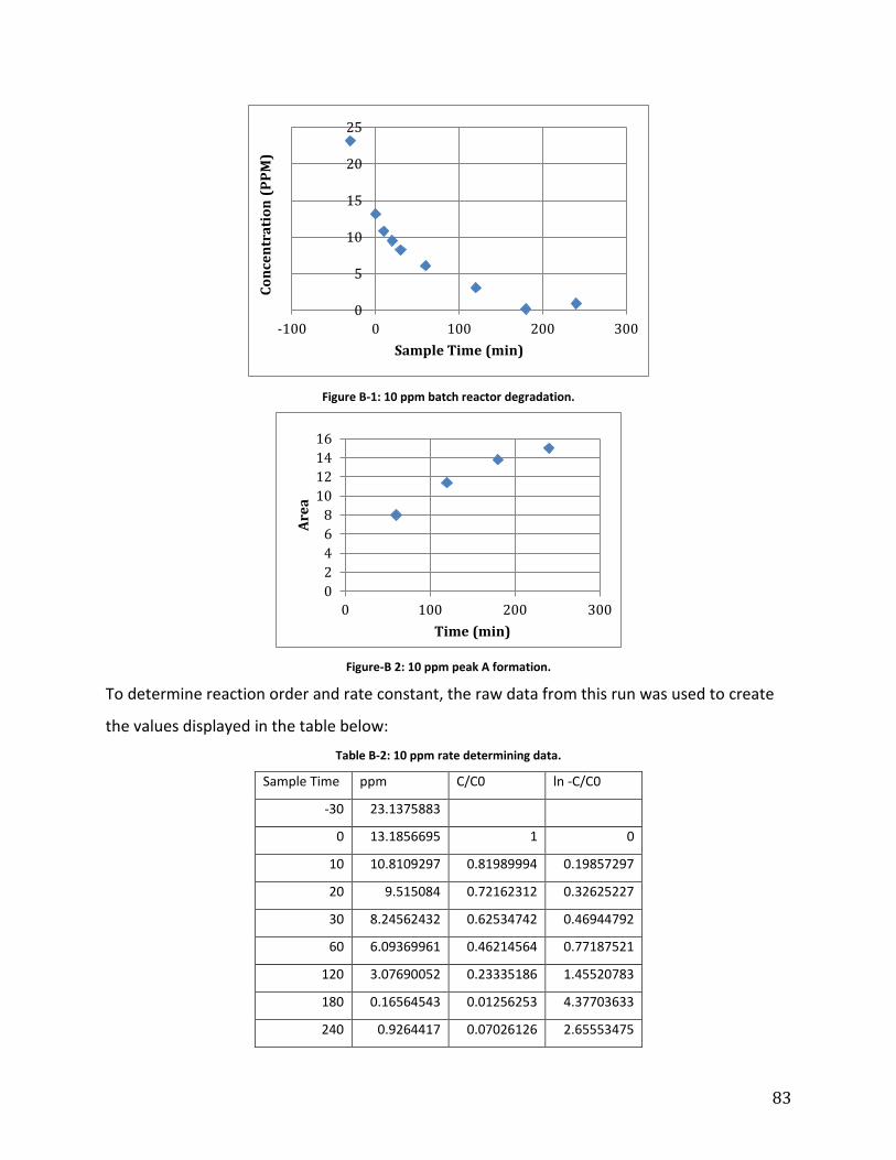
83

Figure B-1: 10 ppm batch reactor degradation.

Figure-B 2: 10 ppm peak A formation.

To determine reaction order and rate constant, the raw data from this run was used to create

the values displayed in the table below:

Table B-2: 10 ppm rate determining data.

Sample Time ppm C/C0 ln -C/C0

-30 23.1375883

0 13.1856695 1 0

10 10.8109297 0.81989994 0.19857297

20 9.515084 0.72162312 0.32625227

30 8.24562432 0.62534742 0.46944792

60 6.09369961 0.46214564 0.77187521

120 3.07690052 0.23335186 1.45520783

180 0.16564543 0.01256253 4.37703633

240 0.9264417 0.07026126 2.65553475

0

5

10

15

20

25

-100 0 100 200 300

Co

nce

ntr

ati

on

(P

PM

)

Sample Time (min)

0

2

4

6

8

10

12

14

16

0 100 200 300

Are

a

Time (min)

84

The data from the table above was used to produce a graph of time vs. –ln(d[CP]) so the graph

would be linear. A line of best fit was created for this graph, pictured below:

Figure B-3: 10 ppm sample time vs. -ln(d[CP]).

y = 0.0161xR² = 0.9865

0

0.1

0.2

0.3

0.4

0.5

0.6

0 20 40

-ln

(d[C

P])

Minutes

Series1

Linear (Series1)

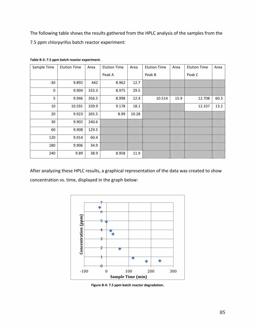
85


7.5 ppm chlorpyrifos batch reactor experiment:

Table B-3: 7.5 ppm batch reactor experiment.

Sample Time Elution Time Area Elution Time

Peak A

Area Elution Time

Peak B

Area Elution Time

Peak C

Area

-30 9.892 442 8.962 12.7

0 9.904 333.3 8.975 29.5

5 9.946 356.5 8.998 12.4 10.514 15.9 12.708 60.3

10 10.591 339.9 9.178 18.1 12.337 13.2

20 9.923 265.5 8.99 10.28

30 9.902 240.6

60 9.908 129.5

120 9.914 60.4

180 9.906 34.9

240 9.89 38.9 8.958 11.9



Figure B-4: 7.5 ppm batch reactor degradation.

0

1

2

3

4

5

6

7

-100 0 100 200 300

Co

nce

ntr

ati

on

(p

pm

)

Sample Time (min)

86

When these samples were analyzed using the HPLC, additional peaks appeared along with the

chlorpyrifos peaks. A graph of area vs. elution of these peaks is pictured below:

Figure B-5: 7.5 ppm peak A formation.

To determine reaction order and rate constant, the raw data from this run was used to create

the values displayed in the table below:

Table B-4: 7.5 ppm rate determining data.

Sample Time ppm C/C0 ln (-C/C0) r0

0 4.88580726 1 0

20 3.89193468 0.797 0.22742814 0.05

30 3.52692838 0.722 0.32590718 0.068

60 1.89832596 0.389 0.9453621 0.149

120 0.88539682 0.181 1.70805388 0.2

180 0.51159518 0.105 2.25655616 0.219

240 0.57023073 0.117 2.14804873 0.216

0

10

20

30

40

50

60

70

-40 -20 0 20 40

Are

a

TIme (min)

Peak A

Peak B

Peak C

87

The data from the table above was used to produce a graph of time vs. –ln(d[CP]) so the graph

would be linear. A line of best fit was created for this graph, pictured below:

Figure B-6: 7.5 ppm sample time vs. ln(d[CP]).

The values produces in the table below were used to produce a graph to find α:

Table B-5: Data to determine alpha.

dCa dt ln(-dCa/dt) ln(Ca)

-1.5934211 30 -2.935314 1.59

-0.9938726 20 -3.0018785 1.36

-0.3650063 10 -3.3104257 1.26

-1.6286024 30 -2.9134751 0.64

-1.0129291 60 -4.0814983 -0.1

-0.3738016 60 -5.0783746 -0.7

A line of best fit was created for this graph of ln(-dCa/dt) vs. ln(Ca), shown below, and the slope

of this line, α, was found to be 0.9399:

y = 0.011xR² = 0.8981

0

0.5

1

1.5

2

2.5

3

0 100 200 300

-ln

(d[C

P])

Minutes

Series1

Linear(Series1)

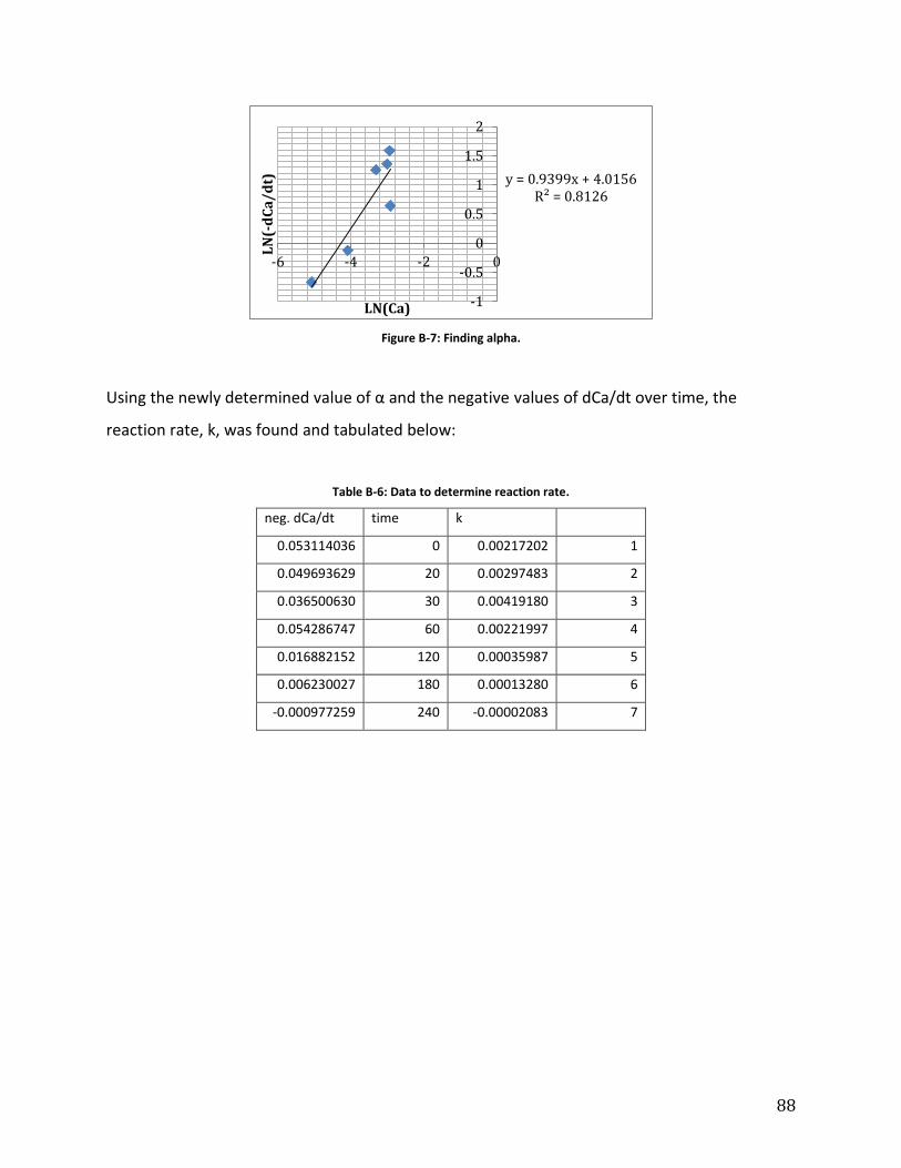
88

Figure B-7: Finding alpha.

Using the newly determined value of α and the negative values of dCa/dt over time, the

reaction rate, k, was found and tabulated below:

Table B-6: Data to determine reaction rate.

neg. dCa/dt time k

0.053114036 0 0.00217202 1

0.049693629 20 0.00297483 2

0.036500630 30 0.00419180 3

0.054286747 60 0.00221997 4

0.016882152 120 0.00035987 5

0.006230027 180 0.00013280 6

-0.000977259 240 -0.00002083 7

y = 0.9399x + 4.0156R² = 0.8126

-1

-0.5

0

0.5

1

1.5

2

-6 -4 -2 0L

N(-

dC

a/

dt)

LN(Ca)

89

These k values over time were graphed below:

Figure B-8: Reaction rate k vs. time.

-0.0005

0

0.0005

0.001

0.0015

0.002

0.0025

0.003

0.0035

0.004

0.0045

1 2 3 4 5 6 7

90

Below are the results and degradation curves obtained from the 5 ppm chlorpyrifos batch

reactor experiment:

Table B-7: 5 ppm batch reactor experiment.

Sample Time Elution Time Area

-30 9.854 704.26

0 9.842 486.4

10 9.839 423.1

15 9.842 405.1

20 9.852 371.5

30 9.82 336.4

60 9.845 234.2

120 9.829 131.9

180 9.809 65.7

240 9.84 45.9



Figure B-9: 5 ppm batch reactor degradation.

0

2

4

6

8

10

12

-100 0 100 200 300

Co

nce

ntr

ati

on

(p

pm

)

Sample Time (min)

91

The concentration of chlorpyrifos at each time interval was divided by the initial concentration

and the natural logs were taken for those values. These results are tabulated below:

Table B-8: 5 ppm rate determining data.

Sample Time ppm C/C0 ln(C/C0)

-30 10.3236682

0 7.13008297 1 0

10 6.20217538 0.8698602 0.13942277

15 5.9383154 0.83285362 0.18289738

20 5.44577677 0.76377467 0.26948247

30 4.93124982 0.69161184 0.3687304

60 3.4331115 0.48149671 0.73085588

120 1.93350729 0.27117599 1.30498727

180 0.96308892 0.13507401 2.00193241

240 0.67284294 0.09436678 2.36056621

A graph of sample time vs. –ln(d[CP]) is shown below:

Figure B-10: 5 ppm sample time vs. -ln(d[CP]).

y = 0.0105xR² = 0.9904

0

0.5

1

1.5

2

2.5

3

0 100 200 300

-ln

(d[C

P])

Sample Time

Series1

Linear(Series1)

92

B.3 - TOC Analysis

The TOC (Total Organic Carbon) analyzer required samples without nitrogen, meaning all

samples created with acetonitrile were incapable of analysis due to the organic nature of

acetonitrile. The samples created in double deionized water at concentrations of 2 ppm

chlorpyrifos and lower could be run through the TOC analyzer without interference from

solvent.

93

Appendix C – Batch & CPC Reactor HPLC Results Run with Water

C.1 – Batch Reactor Results



Table C-1: 1.5 ppm batch reactor experiment.

Sample Time Time Area ppm

-30 10.157 37 0.55028407

0 10.159 24.6 0.36586454

5 10.153 20.8 0.30934888

10 10.163 16.6 0.2468842

20 10.154 12.2 0.18144502

30 10.177 11.8931 0.17688063

60 10.17 9.7 0.14426366

120 10.163 7.5 0.11154407



Figure C-1: 1.5 ppm batch reactor degradation.

0

0.1

0.2

0.3

0.4

0.5

0.6

-50 0 50 100 150

CP

Co

nce

ntr

ati

on

(p

pm

)

Sample Time (min)

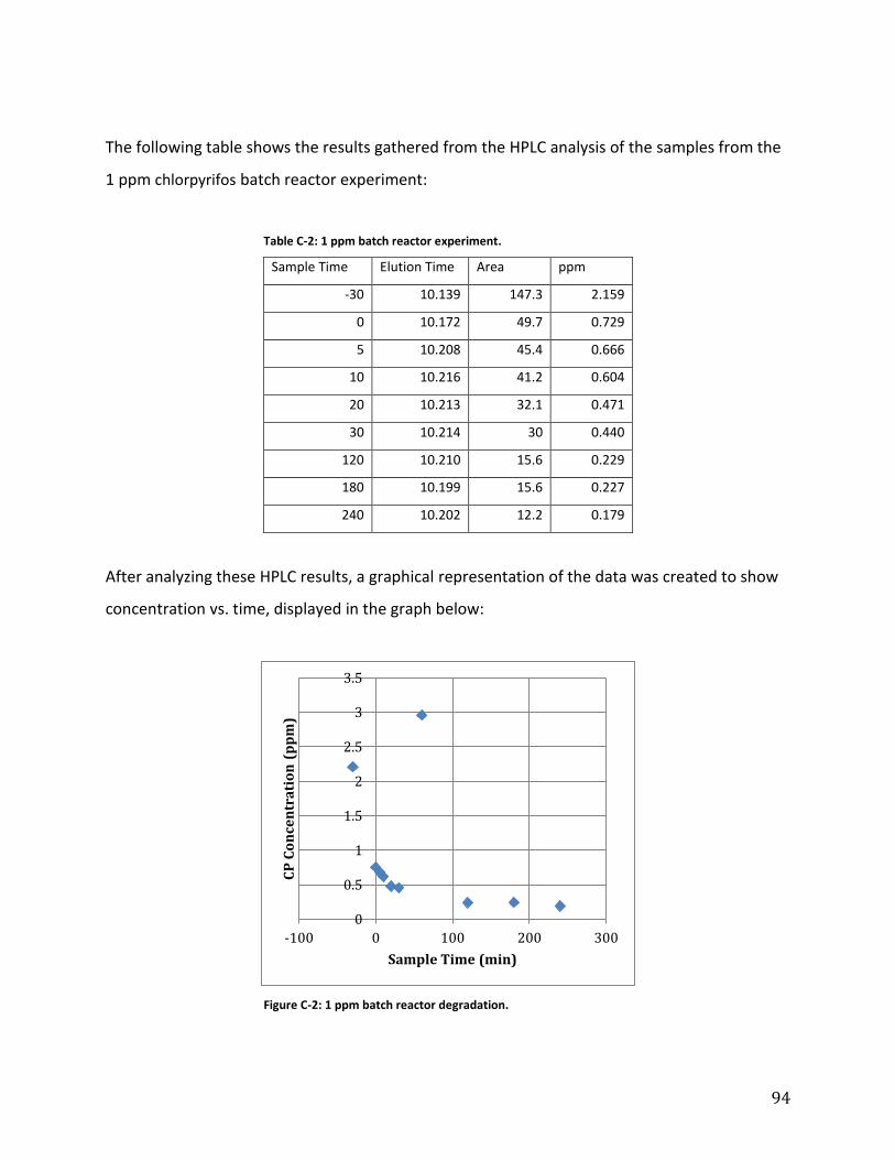
94


1 ppm chlorpyrifos batch reactor experiment:

Table C-2: 1 ppm batch reactor experiment.

Sample Time Elution Time Area ppm

-30 10.139 147.3 2.159

0 10.172 49.7 0.729

5 10.208 45.4 0.666

10 10.216 41.2 0.604

20 10.213 32.1 0.471

30 10.214 30 0.440

120 10.210 15.6 0.229

180 10.199 15.6 0.227

240 10.202 12.2 0.179



Figure C-2: 1 ppm batch reactor degradation.

0

0.5

1

1.5

2

2.5

3

3.5

-100 0 100 200 300

CP

Co

nce

ntr

ati

on

(p

pm

)

Sample Time (min)

95



Table C-3: 0.5 ppm batch reactor experiment.

Sample Time Elution Time Area Elution Time Area ppm

-30 4.813 18 10.029 34.4 0.51161546

5 4.81 18.1 10.021 10.2 0.15169993

10 4.815 13.7 10.041 9.7 0.14426366

20 4.815 18.3 10.041 9.1 0.13534014

30 4.814 18.5 10.044 6.3 0.09369702

60 4.817 13.8 10.055 4 0.05949017

120 4.816 16.1 N/A 2 0.02974508



Figure C-3: 0.5 ppm batch reactor degradation.

0

0.1

0.2

0.3

0.4

0.5

0.6

-50 0 50 100 150

CP

Co

nce

ntr

ati

on

(p

pm

)

Time (min)

96

C.2 – CPC Reactor Results


1.0 ppm chlorpyrifos CPC reactor experiment:

Table C-4: 1.0 ppm CPC reactor experiment.

time elution area

-30 10.199 12.3

0 10.208 8.3

10 10.210 10

20 10.210 8.1

30 10.191 5

60 10.203 5.4

120 N/A N/A

180 N/A N/A

240 10.210 N/A

300 10.225 N/A



Figure C-4: 1.0 CPC reactor degradation.

0

0.02

0.04

0.06

0.08

0.1

0.12

0.14

0.16

0.18

0.2

-40 -20 0 20 40 60 80

Co

nce

ntr

ati

on

(p

pm

)

Time (min)

97


0.5 ppm chlorpyrifos CPC reactor experiment:

Table C-5: 0.5 ppm CPC reactor experiment.

Sample Time Elution Time Area

-30 10.126 43.4

0 10.095 6.9

10 10.064 6.1

20 10.039 5.4

30 10.029 5.3

45 10.029 5.1

60 10.008 5.7

90 10.015 N/A

120 9.997 N/A

150 9.993 N/A

180 9.982 N/A

195 9.988 N/A

210 9.976 N/A

225 9.972 N/A

240 9.981 N/A

255 9.975 N/A

270 9.988 N/A

285 9.98 N/A

300 10.012 N/A

98



Figure C-5: 0.5 ppm CPC reactor degradation.

0

0.05

0.1

0.15

0.2

0.25

0.3

0.35

-40 -20 0 20 40 60 80

Co

cne

ntr

ati

on

(p

pm

)

Sample Time (min)

99

Appendix D – Batch Reactor and CPC Reactor TOC Results

D.1 – Batch Reactor Results

The samples taken from the batch reactor experiment underwent TOC analysis. Below are the

tabulated results of the total carbon over time from the 2 ppm run:

Table D-1: 2.0 ppm batch reactor TOC results.

Sample Time Concentration of Total Carbon

c(TC) mg/L

-30 222.7

0 304

5 599.8

10 351.3

20 726.3

30 463.9

60 59.98

120 5.14

180 4.773

240 4.4

These results are represented graphically below:

Figure D-1: 2.0 ppm Total Carbon vs. Sample Time.

0

100

200

300

400

500

600

700

800

-100 0 100 200 300

To

tal

Ca

rbo

n (

mg

/L

)

Sample Time (min)

100

The samples taken from the batch reactor experiment underwent TOC analysis. Below are the


Table D-2: 1.0 ppm batch reactor TOC results.


c(TC) mg/L

-30 4.24

0 61.26

5 54.9

10 54.88

20 54.39

30 53.83

60 52.06

120 49.25

180 44.57

240 40.26



0

10

20

30

40

50

60

70

-50 0 50 100 150 200 250 300

To

tal

Ca

rbo

n (

mg

/L

)

Sample Time (min)

101

D.2 – CPC Reactor Results

The samples taken from the CPC reactor experiment underwent TOC analysis. Below are the


Table D-3: 2.0 ppm CPC reactor TOC results.


c(TC) mg/L

-30 0

0 1.08

10 1.62

20 2.44

30 3.44

60 2.1

90 2.56

120 2.34

180 1.71

240 1.53



0

0.5

1

1.5

2

2.5

3

3.5

4

-50 0 50 100 150 200 250 300

To

tal

Ca

rbo

n (

mg

/L

)

Sample Time (min)

102





c(TC) mg/L

-30 0

0 106.3

10 0

20 0

30 0

60 0

120 161.5

180 108.3

240 503.8

300 59.42



0

100

200

300

400

500

600

-100 0 100 200 300 400

To

tal

Ca

rbo

n (

mg

/L

)

Sample Time (min)

103


tabulated results of the total carbon over time from the 0.5 ppm run:



c(TC) mg/L

-30 0

0 41.93

10 16.06

20 0

30 0

45 0

60 0

90 0

120 0

150 0

180 0

240 0

300 0



0

5

10

15

20

25

30

35

40

45

-100 0 100 200 300 400

To

tal

Ca

rbo

n (

mg

/L

)

Sample Time (min)

104

Appendix E – Preparing 1F Solution

1. Add 15 mL of titanium tetraisopropoxide (TTIP) to a beaker containing absolute ethanol

(1.25 mL).

2. Dissolve 1 mL of 70% perchloric acid (HClO4) in 90 mL of deionized water in another

beaker.

3. Add the second solution of HClO4 and water drop wise to the first solution of TTIP and

absolute ethanol.

4. Amorphous hydratized TiO2 is a product of the exothermic reaction that occurred from

the mixing of these two solutions.

5. Reflux the solution at 100 °C to allow for the crystallization and degradation of TiO2

particles to occur.

105

Appendix F – Determination of Treatment Efficiency

F.1 - Experimental Treatment Efficiency Determination

Using concentrations of chlorpyrifos at T=0 min and T=120 min the treatment efficiency after

two hours can be determined for each of the four CPC reactor experiments.

Table F: Treatment efficiency after two hours.

Experiment # Chlorpyrifos

concentration at T=0

Chlorpyrifos

concentration at T=120

Treatment Efficiency

1 .05 ppm 0 ppm 1

2 .067 0 ppm 1

3 .121 0 ppm 1

4 .186 .080 ppm .57

Average .8917

F.2 - Theoretical Treatment Efficiency Determination

Theoretical treatment efficiency was determined through the use of the first order reaction

equation, the rate constant found for the photocatalytic degradation of chlorpyrifos using

UV/TiO2, and a retention time of two hours.

[Equation 6]

Where k = Reaction rate constant

T = Retention time

=90.9%

As can be clearly seen the experimental value and the theoretical value for treatment efficiency

are within 2% of one another, indicating that experimental values were accurate.

Eff1

ek t1

E f f1

e( 0 .0 21 2 0)

1 .9 0 9

106

Appendix G – LCMS Chromatograms

The following is a compilation of chromatograms received from LCMS analysis. Specifically

contained in this appendix are the chromatograms from which intermediates were identified.

Figure G-1: Chromatogram from 0.5 ppm CPC experiment at T=285 min.

Figure G-2: Elution times 9.316-9.433 min from Figure G-1.

Figure G-3: Elution times 12.969 - 12.965 min From Figure G-1.

Figure G-4: Chromatogram from 2 PPM slurry experiment at T=42 min.

Figure G-5: Elution times 4.708 - 4.909 min from Figure G-4.

107

Appendix H – High Performance Liquid Chromatography (HPLC)

Each experiment containing chlorpyrifos solution was treated as described above. As it was

necessary to determine the amount of chlorpyrifos remaining in solution after TiO2/UV

treatment, a high performance liquid chromatography (HPLC) instrument (model &

manufacturer information found in Appendix A) was used. As samples were taken over the

course of time for each experiment, aliquots were transferred to individual 2 mL HPLC vials

using Pasteur pipettes. These vials were carefully labeled for organizational aid.

H.1 – HPLC Operation

The following procedure details the parameters used while operating the HPLC machine:

1. The mobile phase consisted of 80% double deionized water and 20% pure acetonitrile.

2. The pump rate of the mobile phase was 1.0 mL per minute.

3. The sample injection volume was 50 L.

4. The run time for each sample was 13 minutes.

5. Sample vials were placed in the auto sampler portion of the machine in order of

increasing sample time.

6. A blank of double deionized water was analyzed preceding each new set of samples.

7. The sequence table in the software was filled according to this order. The method used

was labeled CP1 and each vial was sampled once.

8. The column was installed using two small threaded adapters, one on either end of the

column, which were attached to high pressure lines between the auto sampler and the

diode array detector (DAD) contained in the HPLC machine.

9. The auto sampler, the mobile phase pumps, and the DAD were all switched on using

the Agilent software.

10. The lines and the column were then flushed with double deionized water at a rate of

1.0 mL per minute for 20 minutes.

11. Pressure within the column was allowed to build and become steady between 12 and

14 bars.

12. Once the pressure appeared stable the series was started.

108

H.2 – Analyzing HPLC Results

Results from this instrument were obtained in the form of chromatograms. The wavelengths

from the diode array detector were 200.8, 230, and 290 nm. Peaks indicating the presence of a

compound consistently appear at specific elution times regardless of intensity or concentration.

The peaks corresponding to chlorpyrifos were integrated using the software connected to the

HPLC machine. After determining the area under a peak, the area could then be divided by the

slope of the calibration curve to determine the concentration of chlorpyrifos in the sample.

Once the concentrations of all samples from an experiment had been determined, these values

could be plotted against the corresponding sample times. This graph effectively provided a

degradation curve, which aided in determining treatment efficiency.

109

Appendix I – Slide Coating Procedure Before conducting experiments with the bench scale fixed-film reactor, glass slides were brush-

coated with a titanium silicate solution, known as 397T. The 397T mixture was prepared

following methods developed by Andraž Šuligoj at UNG as described in the section below. The

slide material chosen was critical since the material itself might have the potential to contribute

byproducts to the UV/TiO2 oxidation reaction. Glass slides were chosen to avoid the possibility

of introducing unwanted ions into the solution. Sodium is the only ion that could be produced

as a byproduct of the UV/TiO2 oxidation reaction using glass slides. This effect was avoided by

using temperatures below 200 °C.

I.1 – Titanium Silicate Preparation The following procedure describes the preparation of glass slides coated with 397T solution.

397T was created using a three-step process, after which it was possible to coat the slides. The

preparation of 397T solution first required mixing another formula known as 396W, also

developed by Andraž Šuligoj.

The 396W solution was prepared by adding the following into a 25

mL beaker:

1. 1.86 mL tetraethyl orthosilicate, 98% (Figure I-1)

2. 1.0 mL double deionized water

3. 6.5mL HCl, 37%

A small magnetic stir bar was added to the beaker of solution on a

stirring plate and mixed until homogenous (approximately 45 min).

Figure I-1: tetraethyl orthosilicate (TEOS) solution produced by Acros Organics.

110

Once 396W was completed, the 397T solution was prepared in a 25 mL

beaker as follows:

1. 8.4 mL of 1F (a solution previously prepared by Marko Kete at

UNG on July 2, 2013 - instructions found in Appendix F)

2. 2 mL Levasil 200/30% (Obermeier, Figure I-2)

3. 8 mL absolute ethanol

4. 1.2 mL 396W

This solution was placed on a stirring plate with a magnetic stir bar and

mixed until homogenous (approximately 1 hour).

After the 397T solution was completed, 1.6 g of PC500 TiO2 and 1.6 g of P25 TiO2 (see Figure I-3)

were slowly added over a period of 10 minutes to ensure homogeneous mixing. Equal masses of

both PC500 and P25 were used to ensure maximum surface contact area and crystallinity

structure, as discussed in Chapter 2.6.1 of this report. The final titanium silicate solution was

stirred for an additional 5 minutes then placed in a sonicator for 10 minutes.

Figure I-3: P25 TiO2 and PC500 TiO2.

Figure I-2: Levasil.

111

I.2 – Brush Application When coating glass slides with the homogenous titanium silicate solution detailed above, it was

necessary to ensure that each glass slide was coated with at least 1.0 mg/cm2 of 397T. The

procedure for coating the glass slides with 397T is as follows:

1. Slides were cleaned with ethanol and dried before beginning the coating process.

2. Identification numbers were etched into each glass slide by hand for easy recognition

after coating.

3. Dry slides were weighed prior to coating to obtain the initial weight.

4. A small brush was dipped into the solution and used to paint each slide by hand to

provide a full, even coat on all faces.

5. After each individual slide was coated they were dried with a common hair dryer and

placed in an oven at 150 °C for one hour.

6. The slides were then removed from the oven and weighed.

7. The difference in weight from initial to current coat was divided by the total area of the

coated slide, which effectively provided a measure of coating thickness in units of mass

per area.

8. A second or third coating was added depending on whether the desired thickness of 1.0

mg/cm2 had been achieved.

photocatalytic oxidation for the removal of … oxidation for the removal of chlorpyrifos from...

Documents