philosophy. - cs.swan.ac.ukcsetzer/lectures/computability/03/cpslidesdraft... · the truth of...

CS_226 Computability TheoryCourse Notes, Spring 2003

Anton Setzer

[email protected]

Tel. 01792 51-3368, Room 211

1-1

The Topic of Computability Theory

A:::::::::::::::

computable::::::::::::

function is a function

f : A → B

such that there is a mechanical procedure forcomputing for every a ∈ A the result f(a) ∈ B.

::::::::::::::::::

Computability:::::::::

theory is the study of computablefunctions.

In computablitity theory we explore the limits of thenotion of computability.

1-2

ExamplesDefine exp

:::

: N → N, exp(n) := 2n,

where N = {0, 1, 2, . . .}.exp is computable.However, can we really computeexp(10000000000000000000000000000000000)?

Let String:::::::

be the set of strings of ASCII symbols.

Define a function check::::::

: String → {0, 1} by

check(p) :=

1 if p is a syntactically correctPascal program,

0 otherwise.

Clearly, the function check is computable.

1-3

Examples (Cont.)Define a function terminate

:::::::::::: String → {0, 1},

terminate(p) :=

1 if p is a syntactically correctPascal program, which terminates,

0 otherwise.

Is terminate computable?

1-4

Examples (Cont.)Define a function issortingfun

::::::::::::::

: String → {0, 1},

issortingfun(p) :=

1 if p is a syntactically correctPascal program, which has as inputa list and returns a sorted list,

0 otherwise.

Is issortingfun computable?

1-5

Problems in ComputabilityIn order to understand and answer the questions we have to

Give a precise definition of what computable means.That will be a mathematical definition.Such a notion is particularly important for showingthat certain functions are non-computable.

Then provide evidence that the definition of“computable” is the correct one.

That will be a philosophical argument.

Develop methods for proving that certain functions arecomputable or non-computable.

1-6

Questions Related to The AboveGiven a function f : A → B can be computed,can it be done effectively?(Complexity theory.)

Can the task of deciding a given problem P1 bereduced to deciding another problem P2?(Reducibility theory).

1-7

More Advanced QuestionsThe following is beyond the scope of this module.

Can the notion of computability be extended tocomputations on infinite objects(e.g. streams of data, real numbers,higher typeoperations)?(Higher and abstract computability theory).

What is the relationship between computing (producingactions, data etc.) and proving.

1-8

Three AreasThree Areas are involved in computability theory.

Mathematics.Precise definition of computability.Analysis of the concept.

Philosophy.Verification that notions found are the correct ones.

Computer science.Study of relationship between these concepts andcomputing in the real world.

1-9

IdealisationIn computability theory, one usually abstracts fromlimitations on

time and

space.

A problem will be computable, if it can be solved on an ide-

alised computer, even if it the computation would take longer

than the life time of the universe.

1-10

History of Computability TheoryGottfried Wilhelmvon Leibnitz (1646 – 1716)

Built a first mechanicalcalculator.

Was thinking about amachine formanipulating symbols inorder to determine truthvalues of mathematicalstatements.

Noticed that this requiresthe definition of a preciseformal language.

1-11

History of Computability Theory

David Hilbert(1862 – 1943)

Poses 1900 in hisfamous list “Math-ematical Problems”as 10th problem todecide Diophantineequations.

1-12

History of Computability TheoryHilbert (1928)

Poses the “Entscheidungsproblem” (decisionproblem).

1-13

EntscheidungsproblemHilbert refers to a theory developed by him forformalising mathematical proofs.

Assumes that it is complete and sound, i.e. that itshows exactly all “true” formulae.

Hilbert asks, whether there is an algorithm, whichdecides whether a mathematical formula is aconsequence of his theory.

Assuming his theory is complete and sound, such analgorithm would decide the truth of allmathematical formulae.

The question, whether there is an algorithm for decidingthe truth of mathematical formulae is later called the“Entscheidungsproblem”.

1-14

History of Computability TheoryGödel, Kleene, Post, Turing (1930s)Introduce different models of computation and provethat they all define the same class of computablefunctions.

1-15


Kurt Gödel (1906 – 1978)

1-16


Stephen Cole Kleene(1909 – 1994)

1-17


Emil Post(1897 – 1954)

1-18


Alan Mathison Turing(1912 – 1954)

1-19

History of Computability TheoryGödel (1931) proves in his second incompletenesstheorem:

Every reasonable recursive theory is incomplete, i.ethere is a formula which is neither provable nor itsnegation.Therefore no such theory proves all true formulae.

Recursive functions will be later shown to be thecomputable functions.

Once this is established, it follows that the“Entscheidungsproblem” is unsolvable – an algorithmfor deciding the truth of mathematical formulae wouldgive rise to a complete and sound theory fulfillingGödel’s conditions.

1-20

History of Computability TheoryChurch, Turing (1936) postulate that the models ofcomputation established above define exactly the set ofall computable functions (Church-Turing thesis).

Both establish undecidable problems and conclude thatthe Entscheidungsproblem is unsolvable, even for aclass of very simple formulae.

Church shows the undecidability of equality in theλ-calculus.Turing shows the unsolvability of the halting problem.That problem turns out to be the most importantundecidable problem.

1-21


Alonzo Church (1903 - 1995)

1-22

History of Computability TheoryPost (1944) studies degrees of unsolvability. This is thebirth of degree theory.

In degree theory one devides problems into groups(“

::::::::::

degrees”) of problems, which are reducible to eachother.

:::::::::::::

Reducible means essentially “relative computable”.

Degrees can be ordered by using reducibility asordering.

The question in degree theory is: what is the structureof degrees?

1-23

Degrees

computable

Degree

Reducible to

problems

1-24


Yuri VladimirovichMatiyasevich (∗ 1947)

Solves 1970 Hilbert’s10th problem nega-tively: The solvabilityof Diophantine equa-tions is undecidable.

1-25


Stephen Cook(Toronto)

Cook (1971) intro-duces the complexityclasses P and NPand formulates theproblem, whetherP 6= NP.

1-26

Current StateThe problem P 6= NP is still open. Complexity theoryhas become a big research area.

Intensive study of computability on infinite objects (e.g.real numbers, higher type functionals) is carried out(e.g. Dr. Berger in Swansea).

Computability on inductive and co-inductive data typesis studied.

Research on program synthesis from formal proofs (e.g.Dr. Berger in Swansea).

1-27

Current StateConcurrent and game-theoretic models of computationare developed (e.g. Prof. Moller in Swansea).

Automata theory further developed.

Alternative models of computation are studied(quantum computing, genetic algorithms).

· · ·

1-28

Name “Computability Theory”The original name was recursion theory, since themathematical concept claimed to cover exactly thecomputable functions is called “recursive function”.

This name was changed to computability theory duringthe last 10 years.

Many books still have the title “recursion theory”.

1-29

Administrative IssuesLecturer:Dr. A. SetzerDept. of Computer ScienceUniversity of Wales SwanseaSingleton ParkSA2 8PPUKRoom: Room 211, Faraday BuildingTel.: (01792) 513368

Fax. (01792) 295651

Email [email protected]

Home page: http://www.cs.swan.ac.uk/∼csetzer/

1-30

Assessment:80% Exam.

20% Coursework.

1-31

Course home pageLocated athttp://www.cs.swan.ac.uk/∼csetzer/lectures/computability/03/index.html

There is an open version,

and a password protected version.

The password is _____________.

1-32

Plan for this Module1. Introduction.

2. Encoding of data types into N.

3. The Unlimited Register Machine (URM) and the haltingproblem.

4. Turing machines.

5. Algebraic view of computability.

6. Lambda-definable functions.

7. Equivalence theorems and the Church-Turing thesis.

1-33

Plan for this Module8. Enumeration of the computable functions.

9. Recursively enumerable predicates and the arithmetichierarchy.

10. Reducibility.

11. Computational complexity.

1-34

Aims of this ModuleTo become familiar with fundamental models ofcomputation and the relationship between them.

To develop an appreciation for the limits of computationand to learn techniques for recognising unsolvable orunfeasible computational problems.

To understand the historic and philosophicalbackground of computability theory.

To be aware of the impact of the fundamental results ofcomputability theory to areas of computer science suchas software engineering and artificial intelligence.

1-35

Aims of this ModuleTo understand the close connection betweencomputability theory and logic.

To be aware of recent concepts and advances incomputability theory.

To learn fundamental proving techniques like inductionand diagonalisation.

1-36

LiteratureCutland: Computability.

Lewis/Papadimitriou:Elements of the Theory of Computation.

Sipser: Introduction to the Theory of Computation.

Martin: Introduction to Languages and the Theory ofComputation.

Hopcroft/Motwani/Ullman: Introduction to AutomataTheory, Languages, and Computation.

Book on automata theory/context free grammars.

Hindley: Basic Simple Type Theory.Best book on the λ-calculus.

1-37

LiteratureVelleman: How To Prove It.

Basic mathematics.

Griffor (Ed.): Handbook of Computability Theory.Expensive. Postgraduate level.

1-38

Section 2

Encoding of Data Types into N

How to encode other data types into N.

Computability on N covers many other data types aswell.

2-39

Number of ElementsNotation 2.1If A is a finite set, let |A| be the number of elements in A.

Remark 2.2

One sometimes writes #A for |A|.

2-40

Cardinality of Finite SetsIf A and B are finite sets, then |A| = |B|, if and only if thereis a bijection between A and B:

Bijection exists

a

b

c

d

e

f

No Bijection?

a

b

c

d

e

2-41

Cardinality of Finite Sets

No Bijection?

a

b

c

d

e

2-42

Cardinality of SetsDefinition 2.3Two sets A and B have the

:::::::

same::::::::::::::

cardinality, A ' B:::::::

, if

there exists a bijection between A and B:if there exists functions f : A → B and g : B → A which areinverse with each other:

∀x ∈ A.g(f(x)) = x and ∀x ∈ B.f(g(x)) = x

Remark 2.4

If A and B are finite sets, then A ' B if and only A and B

have the same number of elements.

2-43

' as an Equivalence RelationLemma 2.5' is an equivalence relation, i.e. for all sets A, B, C wehave:

(a) Reflexivity. A ' A.

(b) Symmetry. If A ' B, then B ' A.

(c) Transitivity. If A ' B and B ' C, then A ' C.

Proof:(a): The function id : A → A, id(a) = a is a bijection.(b): If f : A → B is a bijection, so is its inverse f−1.

(c): If f : A → B and g : B → C are bijections, so is the

composition g ◦ f : A → C.

2-44

Cardinality of the Power SetTheorem 2.6A set A and its power set P(A) := {B | B ⊆ A} never havethe same cardinality:

A 6' P(A)

2-45

Proof of A 6' P(A)

A typical diagonalisation argument.

First consider the case A = N.

We show that there is no bijection f : N → P(N).

Assume f were such a bijection.

We define a set C ⊆ N s.t. C 6= f(n) for every n ∈ N.

C = f(n) will be violated at element n:If n ∈ f(n), we add n not to C, thereforen ∈ f(n) ∧ n 6∈ C.If n 6∈ f(n), we add n to C, therefore n 6∈ f(n)∧ n ∈ C.

We will in the following consider as an example anarbitrary function f : N → P(N) and show how toconstruct a set C s.t. f(n) 6= C for all n ∈ N.

2-46

Example

f(0) = { 0, 1, 2, 3, 4, . . . }f(1) = { 0, 1, 2, 4, . . . }f(2) = { 1, 2, 3, . . . }f(3) = { 0, 1, 3, 4, . . . }

· · ·C = { 0, 1, 2, 3, . . . }

We were going through the diagonal in the above matrix.

Therefore this proof is called a::::::::::::::::::::

diagonalisation::::::::::::::

argument.

2-47

Proof of A 6' P(A)

So we define

C := {n ∈ N | n 6∈ f(n)} .

C = f(n) is now violated at element n:

If n ∈ C , then n 6∈ f(n).

If n 6∈ C, then n ∈ f(n).

C is not in the image of f , a contradiction.

2-48

Proof of A 6' P(A)

In short, the above argument for A = N reads as follows:Assume f : N → P(N) is a bijection.Define

C := {n ∈ N | n 6∈ f(n)} .

C is in the image of f .Assume C = f(n).Then we have

n ∈ CDefinition of C⇔ n 6∈ f(n)

C=f(n)⇔ n 6∈ C

a contradiction

2-49

General SituationFor general A, the proof is almost identical:Assume f : A → P(A) is a bijection.We define a set C, s.t. C = f(a) is violated for a:

C := {a ∈ A | a 6∈ f(a)}C is in the image of f .Assume C = f(a). Then we have

a ∈ CDefinition of C⇔ a 6∈ f(a)

C=f(a)⇔ a 6∈ C

a contradiction

2-50

Countable SetsDefinition 2.7

A set A is:::::::::::::

countable, if it is finite or A ' N.

A set, which is not countable, is called::::::::::::::::

uncountable.

2-51

Examples of (Un)countable SetsN is countable.

Z := {. . . ,−2,−1, 0, 1, 2, . . .} is countable.We can enumerate the elements of Z in the followingway:0,−1,+1,−2,+2,−3,+3,−4, +4, . . ..So we have the following map:0 7→ 0, 1 7→ −1, 2 7→ 1, 3 7→ −2, 4 7→ 2, etc.This map can be described as follows:g : N → Z,

g(n) :=

{n2 if n is even,−n+1

2 if n is odd.

Exercise: Show that g is bijective.

2-52

Examples of (Un)countable SetsP(N) is uncountable.

P(N) is not finite.N 6' P(N).

P({1, . . . , 10}) is countable.Since it is finite.

2-53

Characterisation of Countable SetsLemma 2.8A set A is countable, if and only if there is an injective mapg : A → N.

Remark 2.9

Intuitively, Lemma 2.8 expresses: A is countable, if we can

assign to every element a ∈ A a unique code f(a) ∈ N. It is

not required that each element of N occurs as a code.

2-54

Proof of Lemma 2.8“⇒”:Assume A is countable.Show there is an injective f : A → N.

Case A is finite:Let A = {a0, . . . , an}, where ai are different.We can define f : A → N, ai 7→ i.f is injective.

Case A is infinite:A is countable, so there is a bijection from A into N,which is therefore injective.

2-55

Proof of Lemma 2.8“⇐”: Assume f : A → N is injective.Show A is countable.If A is finite, we are done.Assume A is infinite. Then f is for instance something asfollows:

a

b

c

d

0

1

2

3

4

5

6

7

8

9

fA N

2-56

Proof of Lemma 2.8In order to get a bijection g : A → N, we need to jump overthe gaps in the image of f :

a

b

c

d

0

1

2

3

4

5

6

7

8

9

0

1

2

3

A N Nf

g

2-57

Proof of Lemma 2.8

a

b

c

d

0

1

2

3

4

5

6

7

8

9

0

1

2

3

A N Nf

g

f(a) = 1, which is the element number 0 in the image off .g should instead map a to 0.

2-58

Proof of Lemma 2.8

a

b

c

d

0

1

2

3

4

5

6

7

8

9

0

1

2

3

A N Nf

g

f(b) = 4, which is the element number 1 in the image off .g should instead map b to 1. Etc.

2-59

Proof of Lemma 2.8

a

b

c

d

0

1

2

3

4

5

6

7

8

9

0

1

2

3

A N Nf

g

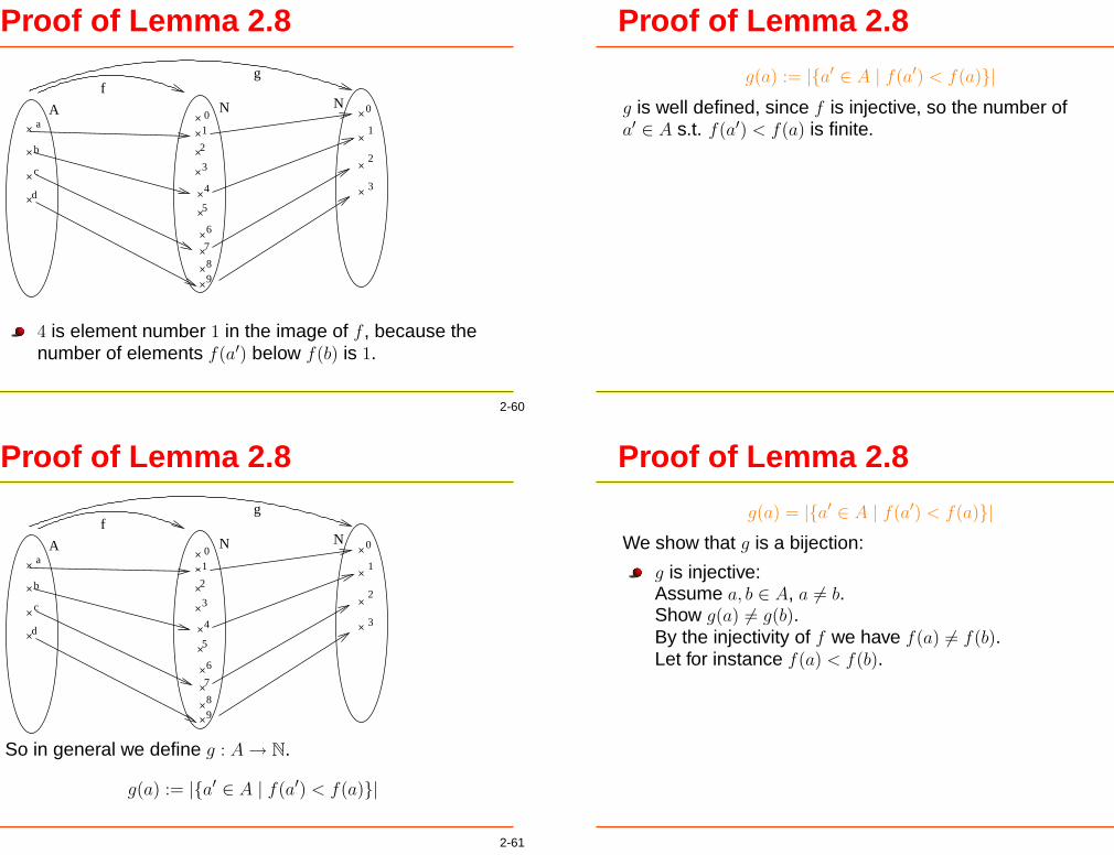
1 is element number 0 in the image of f , because thenumber of elements f(a′) below f(a) is 0.

4 is element number 1 in the image of f , because thenumber of elements f(a′) below f(b) is 1.

2-60

Proof of Lemma 2.8

a

b

c

d

0

1

2

3

4

5

6

7

8

9

0

1

2

3

A N Nf

g

4 is element number 1 in the image of f , because thenumber of elements f(a′) below f(b) is 1.

2-60

Proof of Lemma 2.8

a

b

c

d

0

1

2

3

4

5

6

7

8

9

0

1

2

3

A N Nf

g

So in general we define g : A → N.

g(a) := |{a′ ∈ A | f(a′) < f(a)}|

2-61

Proof of Lemma 2.8

g(a) := |{a′ ∈ A | f(a′) < f(a)}|g is well defined, since f is injective, so the number ofa′ ∈ A s.t. f(a′) < f(a) is finite.

2-62

Proof of Lemma 2.8

g(a) = |{a′ ∈ A | f(a′) < f(a)}|We show that g is a bijection:

g is injective:Assume a, b ∈ A, a 6= b.Show g(a) 6= g(b).By the injectivity of f we have f(a) 6= f(b).Let for instance f(a) < f(b).

2-63

Proof of Lemma 2.8

.

.

.

.

.

.

.

.

.

.

.

.g(b)

g(a)

A

fg

NN

.

.

.

b

f(b)

.

.

.f(a)

.

.

.

.

.

.a

.

.

.

Then

{a′ ∈ A | f(a′) < f(a)}⊂6= {a′ ∈ A | f(a′) < f(b)} ,

therefore

g(a) = |{a′ ∈ A | f(a′) < f(a)}| < |{a′ ∈ A | f(a′) < f(b)}| = g(b) ,

g(a) 6= g(b).

2-64

Proof of Lemma 2.8

.

.

.

.

.

.

.

.

.

.

.

.g(b)

g(a)

A

fg

NN

.

.

.

b

f(b)

.

.

.f(a)

.

.

.

.

.

.a

.

.

.

therefore

g(a) = |{a′ ∈ A | f(a′) < f(a)}| < |{a′ ∈ A | f(a′) < f(b)}| = g(b) ,

g(a) 6= g(b).

2-64

Proof of Lemma 2.8

g(a) = |{a′ ∈ A | f(a′) < f(a)}|

g is surjective:We define by induction on k for k ∈ N an element ak ∈ As.t. g(ak) = k. Then the assertion follows:Assume we have defined already a0, . . . , ak−1.

2-65

Proof of Lemma 2.8

A

fg

...

.

.

....

a(k−1)

a0 f(a0)

k−1

0NN

.

.

.f(a(k−1))

.

.

.

.

..

n...

k

a’

a

There exist infinitely many a′ ∈ A, f is injective, so theremust be at least one a′ ∈ A s.t. f(a′) > f(ak−1).

Let n be minimal s.t. n = f(a) for some a ∈ A and n >

f(ak−1).

2-66

Proof of Lemma 2.8

A

fg

...

.

.

....

a(k−1)

a0 f(a0)

k−1

0NN

.

.

.f(a(k−1))

.

.

.

.

..

n...

k

a’

a


Let a be the unique element of A s.t. f(a) = n.

2-66

Proof of Lemma 2.8

A

fg

...

.

.

....

a(k−1)

a0 f(a0)

k−1

0NN

.

.

.f(a(k−1))

.

.

.

.

..

n...

k

a’

a


{a′′ ∈ A | f(a′′) < f(a)} = {a′′ ∈ A | f(a′′) < f(ak−1)} ∪ {ak−1} .

2-66

Proof of Lemma 2.8

A

fg

...

.

.

....

a(k−1)

a0 f(a0)

k−1

0NN

.

.

.f(a(k−1))

.

.

.

.

..

n...

k

a’

a

Therefore g(a) = |{a′′ ∈ A | f(a′′) < f(a)}|= |{a′′ ∈ A | f(a′′) < f(ak−1)}| + 1

= g(ak−1) + 1 = k − 1 + 1 = k .

Let ak := a.

2-67

CorollaryCorollary 2.10

(a) If B is countable and g : A → B injective,then A is countable.

(b) If A is uncountable and g : A → B injective,then B is uncountable.

(c) If B is countable and A ⊆ B, then A is countable.

(d) If A is uncountable and A ⊆ B, then B is uncountable.

Proof: If f : B → N is an injection, so is f ◦ g : A → N. (b):

By (a). Why? (Exercise). (c): By (a). (What is g?; exercise).

(d): By (c). Why? (Exercise).

2-68

Characterisation of Count. Sets, IILemma 2.11

Let A be a non-empty set. A is countable, if and only if there

is a surjection h : N → A.

2-69

Proof of Lemma 2.11“⇒”: Assume A is non-empty and countable.Show there exists a surjection f : N → A.

Case A is finite.Assume A = {a0, . . . , an}.Define f : N → A,

f(k) :=

{ak if k ≤ n ,a0 otherwise .

f is clearly surjective.

2-70

Proof of Lemma 2.11Case A is infinite.A is countable, so there exists a bijection from N to A,which is therefore surjective.

2-71

Proof of Lemma 2.11“⇐”: Assume h : N → A is surjective.Show A is countable.Define g : A → N, g(a) := min{n | h(n) = a}.g(a) is well-defined, since h is surjective:There exists some n s.t. h(n) = a, therefore the minimalsuch n is well-defined.For a ∈ A, h(g(a)) = a, therefore g is injective:If g(a) = g(a′) then a = h(g(a)) = h(g(a′)) = a′.

By Lemma 2.8, A is countable.

2-72

Examples of Uncountable SetsLemma 2.12The following sets are uncountable:

(a) P(N).

(b) F := {f | f : N → {0, 1}}.

(c) G := {f | f : N → N}.

(d) The set of real numbers R.

Proof of (a): P(N) is not finite,

and by Theorem 2.6 N 6' P(N).

2-73

Proof of Lemma 2.12 (b)Proof of Lemma 2.12 (b)Let F := {f | f : N → {0, 1}}.Show F is uncountable.We introduce a bijection between F and P(N).Then by P(N) uncountable it follows F uncountable.Define for A ∈ P(N) the function χA : N → {0, 1},

χA(n) :=

{1 n ∈ A,

0 otherwise.

2-74

Proof of Lemma 2.12 (b)

χA(n) :=

{1 n ∈ A,

0 otherwise.

Example:

0 1 2 3 4 5 6 7 8

A = {0 2, 4, 6, 8, . . .

n

X_A(n)

1

χA is called the::::::::::::::::::

characteristic:::::::::::

function:::

of:::

A.

2-75


χA(n) :=

{1 n ∈ A,

0 otherwise.

χ is a function from P(N) to N → {0, 1}, where we write the

application of χ to an element A as χA instead of χ(A).

2-76


χA(n) :=

{1 n ∈ A,

0 otherwise.

χ has an inverse.Define χ−1 from N → {0, 1} into P(N),for f : N → {0, 1}, χ−1(f) := {n ∈ N | f(n) = 1}.

2-77


χA(n) :=

{1 n ∈ A,

0 otherwise.

χ−1(f) := {n ∈ N | f(n) = 1}

Example:

2, 4, 6, 8, . . . = {0

0 1 2 3 4 5 6 7 8

n

1

f

X^{−1}(f)

2-78


χA(n) :=

{1 n ∈ A,

0 otherwise.

χ−1(f) := {n ∈ N | f(n) = 1}

We show that χ and χ−1 are inverse:χ−1 ◦ χ is the identity: If A ⊆ N, then

χ−1(χA) = {n ∈ N | χA(n) = 1}= {n ∈ N | n ∈ A}= A

2-79


χA(n) :=

{1 n ∈ A,

0 otherwise.

χ−1(f) := {n ∈ N | f(n) = 1}

χ ◦ χ−1 is the identity:If f : N → {0, 1}, then

χχ−1(f)(n) = 1 ⇔ n ∈ χ−1(f)

⇔ f(n) = 1

2-80


χA(n) :=

{1 n ∈ A,

0 otherwise.

χ−1(f) := {n ∈ N | f(n) = 1}

and

χχ−1(f)(n) = 0 ⇔ n 6∈ χ−1(f)

⇔ f(n) 6= 1

⇔ f(n) = 0 .

Therefore χχ−1(f) = f .It follows that χ is bijective and F is uncountable.

2-81

Proof of Lemma 2.12 (c)Proof of Lemma 2.12 (c)Show G := {f | f : N → N} is uncountable.This is the case since

F = {f | f : N → {0, 1}}

is uncountable and F ⊆ G.

2-82

Proof of Lemma 2.12 (d)Proof of Lemma 2.12 (d)Show R is uncountable.By (b), F = {f | f : N → {0, 1}} is uncountable.A first idea is to define a function f0 : F → R,f0(g) = (0.g(0)g(1)g(2) · · · )2.Here the right hand side is a number in binary format.If f0 were injective, then by F uncountable we couldconclude R is uncountable.The problem is that (0.a0a1 · · · ak01111 · · · )2 and(0.a0a1 · · · ak10000 · · · )2 denote the same real number, so f0

is not injective.We modify f0 so that we don’t obtain any binary numbers ofthe form (0.a0a1 · · · ak01111 · · · )2.

2-83

Proof of Lemma 2.12 (d)Define instead f : F → R,f(g) = (0.g(0) 0 g(1) 0 g(2) 0 · · · )2,i.e. f(g) = (0.a0a1a2 · · · )2, where

ak :=

{0 if k is odd,g(k

2) otherwise.

If two sequences (b0b1b2 · · · ) and (c0c1c2 · · · ) do not end in1111 · · · , i.e. are not of the form (d0d1 · · · dl11111 · · · ), then

(0.b0b1 · · · )2 = (0.c0c1 · · · )2 ⇔ (b0b1b2 · · · ) = (c0c1c2 · · · )

2-84

Proof of Lemma 2.12 (d)Therefore

f(g) = f(g′)

⇔ (0.g(0) 0 g(1) 0 g(2) 0 · · · )2 = (0.g′(0) 0 g′(1) 0 g′(2) 0 · · · )2⇔ (g(0) 0 g(1) 0 g(2) 0 · · · ) = (g′(0) 0 g′(1) 0 g′(2) 0 · · · )⇔ (g(0) g(1) g(2) · · · ) = (g′(0) g′(1) g′(2) · · · )⇔ g = g′ ,

f is injective.

2-85

Continuum HypothesisRemark: The above sets have the same cardinality.Question: Is there a set B which has cardinality between N

and R?

I.e. there are injections N → B and B → R,

but no bijections N → B and B → R.

::::::::::::::

Continuum::::::::::::::::

Hypothesis: There exists no such set.

Continuum Hypothesis is independent of set theory.

2-86

Paul Cohen

Paul Cohen(∗ 1934)Showed that the contin-uum hypothesis is inde-pendent of set theory.

2-87

Image of f

Definition 2.23Let f : A → B, A′ ⊆ A.

(a) f [A′]:::::

:= {f(a) | a ∈ A} is called the

::::::::

image:::

of:::

A′:::::::::

under::

f .

(b) The image of A under f is called the::::::::

image:::

of::

f .

2-88

Image of f

A B

a

b

c

d

e

f

g

h

f

2-89

Image of f

A B

a

b

c

d

e

f

g

h

A’

f

Image of A′ under f .

2-89

Image of f

A B

a

b

c

d

e

f

g

h

A’f[A’]

Image of A′ under f .

2-89

Image of f

A B

a

b

c

d

e

f

g

h

f[A]

f

Image of f .

2-89

Injective/Surjective/BijectiveDefinition 2.23Let A, B be sets, f : A → B.

(a) f is:::::::::::

injective or:::

an::::::::::::

injection or::::::::::::::

one-to-one, iff applied to different elements of A has different results:∀a, b ∈ A.a 6= b → f(a) 6= f(b).

(b) f is:::::::::::::

surjective or::

a:::::::::::::

surjection or::::::

onto, ifevery element of B is in the image of f :∀b ∈ B.∃a ∈ A.f(a) = b.

(c) f is:::::::::::

bijective or::

a:::::::::::

bijection or a

::::::::::::::

one-to-one::::::::::::::::::::::

correspondenceif it is both surjective and injective.

2-90

Visualisation of “Injective”If we visualise a function by having arrows from elementsa ∈ A to f(a) ∈ B then we have the following:

A function is injective, if for every element of B there isat most one arrow pointing to it:

a

b

c

d

e

a

b

c

d

e

injective non-injective

2-91

Visualisation of “Surjective”A function is surjective, if for every element of B thereis at least one arrow pointing to it:

a

b

c

d

e

a

b

c

d

f

e

surjective non-surjective

2-92

Visualisation of “Bijective”A function is bijective, if for every element of B there isexactly one arrow pointing to it:

a

b

c

d

e

f

bijective

Note that, since we have a function, for every elementof A there is exactly one arrow originating from there.

2-93

Remark on SequencesA function f : N → A is nothing but an infinite sequence ofelements of A numbered by elements of N, namelyf(0), f(1), f(2), . . ., usually written as (f(n))n∈N.We identify functions f : N → A with infinite sequences ofelements of A.So the following denotes the same mathematical object:

The function f : N → N, f(n) =

{0 if n is odd,1 if n is even.

The sequence (1, 0, 1, 0, 1, 0, . . .).

The sequence (an)n∈N where an =

{0 if n is odd,1 if n is even.

2-94

Partial FunctionsA partial function f : A

∼→ B is the same as a functionf : A → B, but f(a) might not be defined for all a ∈ A.

Key example: function computed by a computerprogram:

Program has some input a ∈ A and possibly returnssome b ∈ B.(We assume that program does not refer to globalvariables).If the program applied to a ∈ A terminates andreturns b, then f(a) is defined and equal to b.If the program applied to a ∈ A does not terminate,then f(a) is undefined.

2-95

Examples of Partial FunctionsOther Examples:

f : R∼→ R, f(x) = 1

x :f(0) is undefined.

g : R∼→ R, g(x) =

√x:

g(x) is defined only for x ≥ 0.

2-96

Definition of Partial FunctionsDefinition 2.24

Let A, B be sets. A partial function f from A to B,written f : A

∼→ B, is a function f : A′ → B for someA′ ⊆ A.A′ is called the

::::::::::

domain:::

of::

f , written as A′ = dom(f).

Let f : A∼→ B.

:::::

f(a):::

is::::::::::

defined, written as f(a) ↓::::::

, if a ∈ dom(f).

f(a) ' b:::::::::

(:::::

f(a):::

is:::::::::::

partially::::::::

equal:::

to::

b)

:⇔ f(a) ↓ ∧f(a) = b.

2-97

Terms formed from Partial FunctionsWe want to work with terms like f(g(2), h(3)), wheref, g, h are partial functions.

Question: what happens if g(2) or h(3) is undefined?There is a theory of partial functions, in whichf(g(2), h(3)) might be defined, even if g(2) or h(3) isundefined.Makes senses for instance for the functionf : N2 ∼→ N, f(x, y) = 0.Theory of such functions is more complicated.

Functions, which are defined, even if some of itsarguments are undefined, are called

::::::::::::

non-strict.

Functions, which are defined only if all of its argumentsare defined are called

:::::::

strict.

2-98

Terms formed from Partial FunctionsIn this lecture, functions will always be strict.

Therefore, a term like f(g(2), h(3)) is defined only, if g(2)and h(3) are defined, and if f applied to the results theresults of evaluating g(2) and h(3) is defined.

f(g(2), h(3)) is evaluated as for ordinary functions: Wefirst compute g(2) and h(3), and then evaluate f appliedto the results of those computations.

2-99

Terms formed from Partial FunctionsDefinition 2.25

For expressions t formed from constants, variables andpartial functions we define t ↓, t ' b:

If t = a is a constant, then t ↓ holds always andt ' b :⇔ a = b.If t = x is a variable, then t ↓ holds always andt ' x :⇔ a = x.

f(t1, . . . , tn) ' b :⇔ ∃a1, . . . , an.t1 ' a1 ∧ · · · ∧ tn ' an

∧f(a1, . . . , an) ' b .

f(t1, . . . , tn) ↓ :⇔ ∃b.f(t1, . . . , tn) ' b

2-100

Terms formed from Partial Functionss ↑:⇔ ¬(s ↓).We define for expressions s, t formed from constantsand partial functions

s ' t :⇔ (s ↓↔ t ↓) ∧ (s ↓→ ∃a, b.s ' a ∧ t ' b ∧ a = b)

:

t:::

is::::::

total means t ↓.

A function f : A∼→ B is

::::::

total, iff ∀a ∈ A.f(a) ↓.

Remark:Total partial functions are ordinary (non-partial) functions.

2-101

QuantifiersRemark:Quantifiers always range over defined elements.So by ∃m.f(n) ' m we mean: there exists a defined m s.t.f(n) ' m.

So from f(n) ' g(k) we cannot conclude ∃m.f(n) ' m un-

less g(k) ↓.

2-102

Remark 2.26Remark 2.26

(a) If a, b are constants, s ' a, s ' b, then a = b.

(b) For all terms we have t ↓⇔ ∃a.t ' a.

(c) f(t1, . . . , tn) ↓⇔ ∃a1, . . . , an.t1 ' a1 ∧ · · ·∧tn ' an

∧f(a1, . . . , an) ↓ .

2-103

Examples

Assume f : N∼→ N, dom(f) = {n ∈ N | n > 0}, f(n) := n + 1

for n ∈ dom(f).Let g : N

∼→ N, dom(g) = {0, 1, 2}, g(n) := n.

f(1) ↓, f(0) ↑, f(1) ' 2, f(0) 6' n for all n.

g(f(0)︸︷︷︸↑

) ↑ , since f(0) ↑.

g(f(1)︸︷︷︸'2

) ↓ , since f(1) ↓, f(1) ' 2, g(2) ↓.

g(f(2)︸︷︷︸'3

) ↑, since f(2) ↓, f(2) ' 3, but g(3) ↑.

2-104

Examples

f : N∼→ N, dom(f) = {n ∈ N | n > 0}, f(n) := n + 1 for

n ∈ dom(f).g : N

∼→ N, dom(g) = {0, 1, 2}, g(n) := n.

g(f(2))︸︷︷︸↑

' f(0)︸︷︷︸↑

, since both expressions are undefined.

g(f(1))︸︷︷︸'2

' f(g(1))︸︷︷︸'2

, since both sides are defined and

equal to 2.

g(f(2))︸︷︷︸↑

6' f(g(1))︸︷︷︸↓

, since the left hand side is undefined,

the right hand side is defined.

2-105

Examples


n ∈ dom(f).g : N

∼→ N, dom(g) = {0, 1, 2}, g(n) := n.

f(f(1))︸︷︷︸'2

6' f(1)︸︷︷︸'3

, since both sides evaluate to different

(defined) values.

2-106

Examples


n ∈ dom(f).g : N

∼→ N, dom(g) = {0, 1, 2}, g(n) := n.

+, · etc. can be treated as partial functions. So forinstance

f(1)︸︷︷︸↓

+ f(2)︸︷︷︸↓

↓, since f(1) ↓, f(2) ↓, and + is total.

f(1)︸︷︷︸'2

+ f(2)︸︷︷︸'3

' 5.

f(0)︸︷︷︸↑

+f(1) ↑, since f(0) ↑.

2-107

Call-By-Value/NameRemark: Strict evaluation of functions corresponds to::::::::::::::::

call-by-value evaluation of functions.

Done in most imperative and some functionalprogramming languages.

When evaluating f(t1, . . . , tn), first evaluate t1, . . . , tn.Then evaluate f applied to the results of this evaluation.

Undefined values corresponds to an infinitecomputation.

If one of the ti is undefined, the computation off(t1, . . . , tn) doesn’t terminate.

2-108

Call-By-Value/NameIn Haskell: “call-by-name” evaluation:ti are evaluated only if they are needed in thecomputation of f .

For instance, if we have f : N2 → N, f(x, y) = x, and t isan undefined term, then with call-by-need, the termf(2, t) can be evaluated to 2, since we never need toevaluate t.

So functions in Haskell are non-strict.

In our setting, functions are strict, so f(2, t) as above isundefined.

2-109

λ-Notationλx.t means in an informal setting the function mappingx to t.E.g.

λx.x + 3 is the function f s.t. f(x) = x + 3.λx.

√x is the function f s.t. f(x) =

√x.

This notation used, if one one wants to introduce afunction without giving it a name.

Domain and codomain not specified – when thisnotation is used, this will be clear from the context.

2-110

Some Standard SetsN is the

::::

set:::

of::::::::::

natural::::::::::::

numbers:

N := {0, 1, 2, . . .} .

Note that 0 is a natural number.When counting, we start with 0:

The 0th element of a sequence is what is usuallycalled the first element:E.g., in x0, . . . , xn−1, x0 is the 0th variable.The first element of a sequence is what is usuallycalled the second element.E.g., in x0, . . . , xn−1, x1 is the first variable.etc.

2-111

Some Standard SetsZ is the

::::

set:::

of:::::::::::

integers:

Z:

:= N ∪ {−x | x ∈ N} .

Q is the::::

set:::

of::::::::::::

rationals, e.g.

Q::

:= {x

y| x, y ∈ Z, y 6= 0} .

R:

is the::::

set:::

of::::::

real::::::::::::

numbers.

2-112

Some Standard SetsIf A, B are sets, then A × B

:::::::is the

::::::::::

product:::

of:::

A::::::

and::

B:

A × B := {(x, y) | x ∈ A ∧ y ∈ B}

If A is a set, k ∈ N, k > 0, thenAk is the

::::

set:::

of:::::::::::

k-tuples::::

of::::::::::::

elements:::

of:::

A, i.e.

Ak := {(x0, . . . , xn−1) | x0, . . . , xk−1 ∈ A} .

We identify A1 with A.So we don’t distinguish between (x) and x.

2-113

Relations, Predicates and SetsA

::::::::::::

predicate on a set A is a property P of elements of A.In this lecture, A will usually be Nk for some k ∈ N,k > 0.

We write P (a):::::

for “predicate P is true for the element a

of A”.

We often write “:::::

P (x)::::::::

holds” for “P (x) is true”.

2-114

Relations, Predicates and SetsWe can use P (a) in formulas. Therefore:

¬P (a):::::::

(“not P (a)”) means that “P (a) is not true”.

P (a) ∧ Q(q):::::::::::::

means that “both P (a) and Q(a) are

true”.P (a) ∨ Q(q):::::::::::::

means that “P (a) or Q(a) is true”.

(Esp., if both P (a) and Q(a) are true, thenP (a) ∨ Q(a) is true as well).∀x ∈ B.P (x)::::::::::::::

means that “for all elements x of the set

B P (x) is true”.∃x ∈ B.P (x)::::::::::::::

means that “there exists an element x of

the set B s.t. P (x) is true”.

2-115

Relations, Predicates and SetsIn this lecture, “relation” is another word for “predicate”.

We identify a predicate P on a set A with {x ∈ A | P (x)}.Therefore predicates and sets will be identified.E.g., if P is a predicate,

x ∈ P::::::

stands for x ∈ {x ∈ A | P (x)},

which is equivalent to P (x),∀x ∈ P.ϕ(x):::::::::::::

for a formula ϕ stands for

∀x.P (x) → ϕ(x).etc.

2-116

Relations, Predicates and SetsAn

:::::::

n-ary::::::::::

relation or predicate on N is a relationP ⊆ Nn.A

:::::::

unary,::::::::

binary,:::::::::

ternary relation on N is a 1-ary, 2-ary,3-ary relation on N, respectively.

An:::::::

n-ary:::::::::::

function on N is a function f : Nn → N.A

:::::::

unary,::::::::

binary,:::::::::

ternary function on N is a 1-ary, 2-ary,3-ary function on N, respectively.

2-117

The “dot”-notation.In expressions like ∀x.A(x) ∧ B(x), the scope of thequantifier (∀x.) is as far as possible:

In ∀x.A(x) ∧ B(x), ∀x. refers toA(x) ∧ B(x).In (A → ∀x.B(x) ∧ C(x)) ∨ D(x), ∀x refersonly to B(x) ∧ C(x):this is the maximum scope possibleIt doesn’t make sense to include “) ∨ D(x)” into thescope.In ∃x.A(x) ∧ B(x), ∃x refers toA(x) ∧ B(x).In (A ∧ ∃x.B(x) ∨ C(x)) ∧ D(x), ∃x refers toB(x) ∨ C(x).

2-118

The “dot”-notation.applies as well to λ-expressions.

λx.x + x is the function taking an x and returningx + x.

2-119

~x, ~y etc.Often need for variables, to which we don’t referexplicitly.Example: Variables x0, . . . , xn−1 in

f(x0, . . . , xn−1, y) =

{g(x0, . . . , xn−1), if y = 0,h(x0, . . . , xn−1), if y > 0.

We abbreviate x0, . . . , xn−1, by ~x.

In general, ~x stands for x0, . . . , xn−1, where n, is clearfrom the context.

2-120

~x, ~y etc.Examples:

f : Nn+1 → N, then in f(~x, y), ~x needs to stand forn arguments.Therefore ~x = x0, . . . , xn−1.If f : Nn+2 → N, then in f(~x, y), ~x needs to stand forn + 1 arguments,so ~x = x0, . . . , xn.If P is an n + 4-ary relation, thenin P (~x, y, z), ~x stands forx0, . . . , xn+1.

Similarly, we write ~y for y0, . . . , yn−1, where n is clearfrom the context.

Similarly for ~z, ~n, ~m, etc.

2-121

Encoding of Sequences into N

We will show how to encode sequences of natural numbers

as natural numbers in a computable way.

2-122

Ak, A∗, A → B

DefinitionLet A, B be sets.

Ak := {(a1, . . . , ak) | a1, . . . , ak ∈ A}. Ak is the set ofk-tuples of elements of A, and is called the:::::::

k-fold:::::::::::::

Cartesian:::::::::::

product.Especially A0 = {()}.

A∗ :=⋃

n∈N Ak.A∗ is the set of tuples of A of arbitrary length, and calledthe

::::::::::::::::

Kleene-Star.

A → B := {f | f : A → B}.A → B is the set of functions from A to B and is calledthe

:::::::::::

function:::::::::

space.

2-123

Ak, A∗, A → B

Remark:A∗ can be considered as the set of strings having letters inthe alphabet A.

2-124

Definition of π

We want to define a bijective function π : N2 → N.π will be called the

:::::::::

pairing:::::::::::

function.Pairs of natural numbers can be enumerated in thefollowing way:

y 0 1 2 3 4

x

0 0 2 5 9 14

1 1 4 8 13 19

2 3 7 12 18 25

3 6 11 17 24 32

4 10 16 23 31 40

2-125

Definition of π

y 0 1 2 3 4

x

0 0 2 5 9 14

1 1 4 8 13 19

2 3 7 12 18 25

3 6 11 17 24 32

4 10 16 23 31 40

π(0, 0) = 0 , π(1, 0) = 1 , π(0, 1) = 2 ,

π(2, 0) = 3 , π(1, 1) = 4 , π(0, 2) = 5 , etc.

2-126

Attempt which failsNote, that the following naïve attempt to enumerate thepairs, fails:

y 0 1 2 3

x

0 π(0, 0) → π(0, 1) → π(0, 2) → π(0, 3) → · · ·1 → → → → · · ·2 → → → → · · ·3 → → → → · · ·4 → → → → · · ·

π(0, 0) = 0, π(0, 1) = 1, π(0, 2) = 2, etc.

We never reach the pair (1, 0).

2-127

Definition of π

y 0 1 2 3 4

x

0 0 2 5

1 1 4

2 3

For the pairs in the diagonal we have the property that x + yis constant.The first diagonal, consisting of (0, 0) only, is given by

x + y = 0.

2-128

Definition of π

y 0 1 2 3 4

x

0 0 2 5

1 1 4

2 3

For the pairs in the diagonal we have the property that x + yis constant.The second diagonal, consisting of (1, 0), (0, 1), is given by

x + y = 1.

2-128

Definition of π

y 0 1 2 3 4

x

0 0 2 5

1 1 4

2 3

For the pairs in the diagonal we have the property that x + yis constant.The third diagonal, consisting of (2, 0), (1, 1), (0, 2), is givenby x + y = 2.

Etc.

2-128

Definition of π

y 0 1 2 3 4

x

0 0 2 5

1 1 4

2 3

If we look in the original approach at the diagonals we seethat following:

The diagonal given by x + y = n, consists of n + 1 pairs:The first diagonal, given by x + y = 0, consists of(0, 0) only, i.e. of 1 pair.

etc.

2-129

Definition of π

y 0 1 2 3 4

x

0 0 2 5

1 1 4

2 3


The diagonal given by x + y = n, consists of n + 1 pairs:The second diagonal, given by x + y = 1, consists of(1, 0), (0, 1), i.e. of 2 pairs.

etc.

2-129

Definition of π

y 0 1 2 3 4

x

0 0 2 5

1 1 4

2 3


The diagonal given by x + y = n, consists of n + 1 pairs:The third diagonal, given by x + y = 2, consisting of(2, 0), (1, 1), (0, 2), i.e. of 3 pairs.etc.

2-129

Definition of π

y 0 1 2 3 4

x

0 0 2 5

1 1 4

2 3 7

3 6

We count the elements occurring before the pair (x0, y0).

We have to count all elements of the previousdiagonals. These are those given by x + y = n forn < x0 + y0.

In the above example for the pair (2, 1), these are thediagonals given by x + y = 0, x + y = 1, x + y = 2.

2-130

Definition of π

x y 0 1 2 3 4

0 0 2 5

1 1 4

2 3 7

3 6

The diagonal, given by x + y = n, has n + 1elements, so in total we have∑x+y−1

i=0 (i + 1) = 1 + 2 + · · · + (x + y) =∑x+y

i=1 i

elements in those diagonals.

A often used formula says∑n

i=1 i = n(n+1)2 .

Therefore, the above is (x+y)(x+y+1)2 .

2-131

Definition of π

y 0 1 2 3 4

x

0 0 2 5

1 1 4

2 3 7

3 6

Further, we have to count all pairs in the currentdiagonal, which occur in this ordering before the currentone. These are y pairs.

Before (2, 1) there is only one pair, namely (3, 0).Before (3, 0) there are 0 pairs.Before (0, 2) there are 2 pairs, namely (2, 0), (1, 1).

2-132

Definition of π

y 0 1 2 3 4

x

0 0 2 5

1 1 4

2 3 7

3 6

Therefore we get that there are in total(x+y)(x+y+1)

2 + y pairs before (x, y), therefore the pair

(x, y) is the pair number ( (x+y)(x+y+1)2 + y) in this

order.

2-133

Definition of π

Definition 2.14

π(x, y):::::::

:=(x + y)(x + y + 1)

2+ y (= (

x+y∑

i=1

i) + y)

Exercise: Prove that∑n

i=1 i = n(n+1)2 .

2-134

π is BijectiveLemma 2.15π is bijective.

2-135

Proof of Bijectivity of π

We show π is injective:We prove first that, if x + y < x′ + y′, then π(x, y) < π(x′, y′):

π(x, y) = (

x+y∑

i=1

i) + y < (

x+y∑

i=1

i) + x + y + 1 =

x+y+1∑

i=1

i

≤ (

x′+y′∑

i=1

i) + y′ = π(x′, y′)

2-136


We show π is injective:Assume now π(x, y) = π(x′, y′) and show x = x′ and y = y′.We have by the above x + y = x′ + y′.Therefore

y = π(x, y) − (

x+y∑

i=1

i) = π(x′, y′) − (

x′+y′∑

i=1

i) = y′

and x = (x + y) − y = (x′ + y′) − y′ = x′.

2-137


We show π is surjective:Assume n ∈ N.Show π(x, y) = n for some x, y ∈ N.

The sequence (∑k′

i=1 i)k′∈N is strictly existing.Therefore there exists a k s.t.

a :=k∑

i=1

i ≤ n <k+1∑

i=1

i

2-138


n ∈ N

Show π(x, y) = n for some x, y

a :=k∑

i=1

i ≤ n <k+1∑

i=1

i (∗)

So, in order to obtain π(x, y) = n, we need x + y = k.By y = π(x, y) − ∑x+y

i=1 i, we need to define y := n − a.By k = x + y, we need to define x := k − y.By (∗) it follows 0 ≤ y < k + 1,therefore x, y ≥ 0. Further,π(x, y) = (

∑x+yi=1 i) + y = (

∑ki=1 i) + (n − ∑k

i=1 i) = n.

2-139

Definition of π0, π1

Since π is bijective, we can define π0, π1 as follows:

Definition 2.16Let π0 : N → N and π1 : N → N be s.t.

π0(π(x, y)) = x, π1(π(x, y)) = y.

2-140

π, πi are ComputableRemarkπ, π0, π1 are computable in an intuitive sense.

“Proof:”π is obviously computable.π0(n), π1(n) can be computed, by first searching for a k s.t.k(k+1)

2 ≤ n < (k+1)(k+2)2

and then defining as in the proof of the surjectivity of π

π1(n) := n − k(k+1)2 and π0(n) = k − π1(n).

2-141

Remark 2.17Remark 2.17For all z ∈ N, π(π0(z), π1(z)) = z.

Proof:Assume z ∈ N and show z = π(π0(z), π1(z)).π is surjective, so there exists x, y s.t. π(x, y) = z.Then

π(π0(z), π1(z)) = π(π0(π(x, y)), π1(π(x, y))) = π(x, y) = z.

2-142

Encoding of Nk

Want to encode Nk into N.

(l,m, n) ∈ N3 can be encoded as followsFirst encode (l,m) as π(l,m) ∈ N.Then encode the complete triple as π(π(l,m), n) ∈ N.

So define π3(l,m, n) := π(π(l,m), n).

Similarly (l,m, n, p) ∈ N4 can be encoded as follows:

π4(l,m, n, p) := π(π(π(l,m), n), p).

2-143

Decoding FunctionIf x = π3(l,m, n) = π(π(l,m), n), then we see

l = π0(π0(x)),m = π1(π0(x)),n = π1(x).

So we defineπ3

0(x) = π0(π0(x)),

π31(x) = π1(π0(x)),

π32(x) = π1(x).

2-144

Decoding FunctionSimilarly, if x = π4(l,m, n, p) = π(π(π(l,m), n), p), then wesee

l = π0(π0(π0(x))),m = π1(π0(π0(x))),n = π1(π0(x)).p = π1(x).

So we defineπ4

0(x) = π0(π0(π0(x))),

π41(x) = π1(π0(π0(x))),

π42(x) = π1(π0(x)).

π43(x) = π1(x).

2-145

Definition for General k

In general one defines for k ≥ 1

πk : Nk → N,πk(x0, . . . , xk−1) = π(· · · π(π(x0, x1), x2) · · · xk−1),and for i < kπk

i : N → N,πk

0(x) = π0(· · · π0(︸︷︷︸k − 1 times

x) · · · )

and for 0 < i < k,πk

i (x) = π1( π0(π0(· · · π0(︸︷︷︸k − i − 1 times

x) · · · ))).

An Inductive Definition is as follows:

2-146

Definition 2.18 of πk, πki

(a) We define by induction on k for k ∈ N, k ≥ 1

πk : Nk → N

π1(x) := x

For k > 0 πk+1(x0, . . . , xk) := π(πk(x0, . . . , xk−1), xk)

(b) We define by induction on k for i, k ∈ N s.t. 1 ≤ k,0 ≤ i < k

πki : N → N

π10(x) := x

πk+1i (x) := πk

i (π0(x)) for i < k

πk+1k (x) := π1(x)

2-147

Examplesπ2(x, y) = π(π1(x), y) = π(x, y).

π3(x, y, z) = π(π2(x, y), z) = π(π(x, y), z).

π4(x, y, z, u) = π(π3(x, y, z), u) = π(π(π(x, y), z), u).

π40(u) = π3

0(π0(u)) = π20(π0(π0(u))) = π1

0(π0(π0(π0(u)))) =π0(π0(π0(u))).

π42(u) = π3

2(π0(u)) = π1(π0(u)).

2-148

Lemma 2.19(a) For (x0, . . . , xk−1) ∈ Nk, i < k, xi = πk

i (πk(x0, . . . , xk−1)).

(b) For x ∈ N, x = πk(πk0(x), . . . , πk

k−1(x)).

Proof:Induction on k.Base case k = 0:Proof of (a):Let (x0) ∈ N1.Then π1

0(π1(x0)) = x0.

Proof of (b):Let x ∈ N.Then π1(π1

0(x)) = x.

2-149

Proof of Lemma 2.19Induction step k → k + 1:Assume the assertion has been shown for k.Proof of (a):Let (x0, . . . , xk) ∈ Nk+1.Then

for i < k πk+1i (πk+1(x0, . . . , xk))

= πki (π0(π(πk(x0, . . . , xk−1), xk)))

= πki (πk(x0, . . . , xk−1))

IH= xi

and πk+1k (πk+1(x0, . . . , xk))

= π1(π(πk(x0, . . . , xk−1), xk))

= xk

2-150

Proof of Lemma 2.19Induction step k → k + 1:Assume the assertion has been shown for k.Proof of (b):Let x ∈ N.

πk+1(πk+10 (x), . . . , πk+1

k (x))

= π(πk(πk+10 (x), . . . , πk+1

k−1(x)), πk+1k (x))

= π(πk(πk0(π0(x)), . . . , πk

k−1(π0(x))), π1(x))

IH= π(π0(x), π1(x))

Rem. 2.17= x

2-151

Encoding of N∗

Goal: Encoding N∗ → N.

N∗ = N0 ∪ ⋃n≥n Nn.

N0 = {〈〉},Encode 〈〉 as 0.Encoding of

⋃n≥n Nn:

For n ≥ 1, use πn : Nn → N.Note that m ∈ N is of the form πk(a0, . . . , ak−1) andπl(b0, . . . , bl−1) for different k, l.→ Need to add length to the code.Encode (a0, . . . , an−1) as an element of

⋃n≥1 Nn as

π(n − 1, πn(a0, . . . , an−1)).In order to distinguish it from code of 〈〉, add 1 to it.

In total we obtain a bijection.

2-152

Definition 2.20 of 〈〉, lh, (x)i

(a) Define for x ∈ N∗, 〈x〉 : N as follows:

〈〉 := 0 ,

〈x0, . . . , xk〉 := 1 + π(k, πk+1(x0, . . . , xk))

(b) Define for x ∈ N, the::::::::

length 〈x〉 ∈ N as follows:

lh : N → N ,

lh(0) := 0 ,

lh(x) := π0(x − 1) + 1 if x > 0 .

(c) We define for x ∈ N and i < lh(x), (x)i ∈ N as follows:

(x)i := πlh(x)i (π1(x − 1)).

For lh(x) ≤ i, let (x)i := 0.

2-153

Lemma 2.21Lemma 2.21

(a) lh(〈〉) = 0, lh(〈x0, . . . , xk〉) = k + 1.

(b) For i ≤ k, (〈x0, . . . , xk〉)i = xi.

(c) For x ∈ N, x = 〈(x)0, . . . , (x)lh(x)−1〉.

2-154

Proof of Lemma 2.21 (a)Proof of (a):Show: lh(〈〉) = 0:lh(〈〉) = lh(0) = 0.

Show: lh(〈x0, . . . , xk〉) = k + 1:

lh(〈x0, . . . , xk〉) = π0(〈x0, . . . , xk〉 − 1) + 1

= π0(π(k, · · · ) + 1 − 1) + 1

= k + 1

2-155

Proof of Lemma 2.21 (b)Proof of (b):Show (〈x0, . . . , xk〉)i = xi.lh(〈x0, . . . , xk〉) = k + 1.Therefore

(〈x0, . . . , xk〉)i= πk+1

i (π1(〈x0, . . . , xk〉 − 1))

= πk+1i (π1(1 + π(k, πk+1(x0, . . . , xk)) − 1))

= πk+1i (πk+1(x0, . . . , xk))

Lem 2.19 (a)= xi

2-156

Proof of Lemma 2.21 (c)Proof of (c):Show x = 〈(x0), . . . , (x)lh(x)−1〉.Case x = 0.lh(x) = 0. Therefore 〈(x)0, . . . , (x)lh(x)−1〉 = 〈〉 = 0 = x.Case x > 0.Let x − 1 = π(y, l).Then lh(x) = l + 1, (x)i = πl+1

i (y) and therefore

〈(x)0, . . . , (x)lh(x)−1〉= 〈πl+1

0 (y), . . . , πl+1l (y)〉

= π(πl+1(πl+10 (y), . . . , πl+1

l (y)), l) + 1

Lem 2.19 (a)(a)= π(y, l) + 1

= x

2-157

Theorem 2.22Theorem 2.22

(a) If A is countable, so are Ak, A∗.

(b) If A, B are countable, so are A × B, A ∪ B.

(c) If An are countable sets for n ∈ N, so is⋃

n∈N An.

(d) Q, the set of rational numbers, is countable.

2-158

Proof of Theorem 2.22 (a)Proof of (a):Assume A is countable.We show first that A∗ is countable:There exists f : A → N, f injective.Define f∗ : A∗ → N∗, f∗(a0, . . . , an) = (f(a0), . . . , f(an)).Then f is injective.λx.〈x〉 : N∗ → N is bijective.Therefore (λx.〈x〉) ◦ f∗ : A∗ → N is injective, A∗ is countable.Ak ⊆ A∗, therefore Ak is countable as well.

2-159

Proof of Theorem 2.22 (b)Proof of (b):Assume A, B countable.Show A × B, A ∪ B are countable.If A = ∅ or B = ∅, then A × B = ∅, therefore countable,and A ∪ B = A or A ∪ B = B, therefore countable.

2-160

Proof of Theorem 2.22 (b)A, B are countable.Show A ∪ B, A × B are countable.Assume A,B 6= ∅.Then there exist surjections f : N → A and g : N → B.Then f × g : N2 → A × B, (f × g)(n,m) := (f(n), g(m)) issurjective as well.Further λx.(π0(x), π1(x)) : N → N2 is surjective,therefore as well (f × g) ◦ (λx.(π0(x), π1(x))) : N → A × B.Therefore A × B is countable.Further h : N2 → A ∪ B, h(0, n) := f(n), h(k, n) := g(n) fork > 0, is surjective,therefore as well h ◦ (λx.(π0(x), π1(x))) : N → A ∪ B.

2-161

Proof of Theorem 2.22 (c)Proof of (c):Assume An are countable for n ∈ N.Show A :=

⋃n∈N An is countable as well.

If all An are empty, so is⋃

n∈N An.Assume Ak is non-empty for some k.By replace empty Al by Ak, we get a sequence of sets, s.t.their union is the same as A.

So without loss of generality assume An 6= ∅ for all n.

2-162

Proof of Theorem 2.22 (c)An are countable, An 6= ∅.Show

⋃n∈N An is countable.

An are countable, so there exist fn : N → An surjective.Then f : N2 → A, f(n,m) := fn(m) is surjective as well.Therefore f ◦ (λx.(π0(x), π1(x))) : N → A is as well surjective,A is countable.

2-163

Proof of Theorem 2.22 (d)Proof of (d):Z × N is countable,since Z and N are countable.Let A := {(z, n) ∈ Z × N, n 6= 0}.A ⊆ Z × N, therefore A is countable as well.Since A 6= ∅ is countable, there exists a surjectionf : N → A.Define g : A → Q, g(z, n) := z

n.

g is surjective, therefore as well g ◦ f : N → Q.

Therefore we have defined a surjective function from N onto

Q, Q is countable.

2-164

2.3 Reduction of Computability to N

Goal: Reduce computability on some data types A tocomputability on N.

⇒ No need for a special definition of computabilityon A.

Need:computable function code : A → N,computable function decode : N → A.

2-165

2.3 Reduction of Computability to N

Then from a computable f : A → A we can obtain acomputable f̃ : N → N:

Af - A

N

decode

6

f̃ - N

code

?

In order to recover f from f̃ , we needdecode(code(a)) = a.

2-166

Computable EncodingsInformal DefinitionA data type A has a

:::::::::::::::

computable:::::::::::::

encoding::::::

into::

N,if there exist in an intuitive sense computable functionscode : A → N, and decode : N → Asuch that decode(code(a)) = a for all a ∈ A.

RemarkWe do not require code(decode(n)) = n for every n ∈ N.Every a ∈ A has a unique code in N, i.e. code is injective,expressed by decode(code(a)) = a.But not every n ∈ N needs to be a code for an element of A,code needs not be surjective.

2-167

Encoding of StringsInformal Lemma

If A is a finite non-empty set, then A∗ has a computable en-

coding into N.

2-168

Proof of the Informal LemmaAssume A = {a0, . . . , an}, where ai 6= aj for i 6= j.Define f : A → N, f(ai) = i.Define g : N → A, g(i) = ai for i ≤ n, g(i) = a0 for i > n.f and g are in an intuitive sense computable,therefore as well code : A∗ → N,code(a1, . . . , an) = 〈f(a1), . . . , f(an)〉,and decode : N → A∗, decode(n) := (g((n)0), . . . , g((n)lh(n)−1)).

2-169

Proof of the Informal Lemmacode(a1, . . . , an) = 〈f(a1), . . . , f(an)〉,decode(n) := (g((n)0), . . . , g((n)lh(n)−1)).We show decode(code(x)) = x for x ∈ A∗:Let x = (a1, . . . , an)

decode(code(x)) = decode(code(a1, . . . , an))

= decode(〈f(a1), . . . , f(an)〉)= (g(f(a1)), . . . , g(f(an))

= (a1, . . . , an)

= x .

2-170

RemarkAssume A, B have computable encodings codeA : A → N,decodeA : N → A and codeB : B → N, decodeB : N → B.If f : A → B is in an intuitive sense computable, then wecan define an in an intuitive sense computable functionf̃ : N → N, f̃ := codeB ◦ f ◦ decodeA

Af - B

N

decodeA

6

codeA

? f̃ - N

decodeB

6

codeB

?

2-171

Recovering f from f̃

Af - B

N

decodeA

6

codeA

? f̃ - N

decodeB

6

codeB

?

From f̃ we can recover f , since f = decodeB ◦ f̃ ◦ codeA

(easy exercise).

So by considering computability on N we cover computability

on data types with a computable encoding into N as well.

2-172

Sec. 3: The URMA

::::::::

model:::

of:::::::::::::::::

computation consists of a set of partialfunctions together with methods, which describe, howto compute those functions.

Our models of computation will contain allcomputable functions.Aim: an as simple model of computation aspossible:constructs used minimised, while still being able torepresent all computable functions.Makes it easier to show for other models ofcomputation, that the first model can be interpretedin it.Models of computation mainly used for showing thatsomething is non-computable rather than forshowing that something is computable in this model.

3-173

The URMThe URM (the unlimited register machine) is one modelof computation.

Particularly easy.Is a virtual machine, i.e. a description how acomputer would execute its program.Not intended for actual implementation.Is an abstract virtual machine – not intended to besimulated on a computer.Intended as a mathematical model, which is theninvestigated mathematically.Not many programs are actually written in it – oneshows that in principal there is a way of writing acertain program in this language.

3-174

The URMRather difficult to write actual programs for the URM.Low level programming language (only goto)URM idealised machine – no bounds on the amountof memory or execution time

however all values will be finite.Many variants of URM – this URM will be particularlyeasy.

3-175

Description of the URMThe URM consists of

infinitely many registers Ri

can store arbitrarily big natural number;a finite sequence of

:::::::::::::::

instructions I0, I1, I2, . . . In;and a

:::::::::::

program:::::::::::

counter::::

PC.stores a natural number.If content is a number 0 ≤ i ≤ n, PC points toinstruction Ii.If content is outside this range, the program stops.

3-176

The URM

R0 R1 R2 R3 R4 R5 R6 R7 R8 · · ·

I0 I1 I2 · · · In

PC

Execute Instruction

3-177

The URM

R0 R1 R2 R3 R4 R5 R6 R7 R8 · · ·

I0 I1 I2 · · · In

PC

Program has terminated

3-177

URM Instructions3 kinds of

::::::

URM::::::::::::::::

instructions.The

:::::::::::::

successor:::::::::::::::

instruction succ(n), where n ∈ N.

Execution:Add 1 to register Rn.Increment PC by 1.→ execute next instruction or terminate.

The::::::::::::::::

predecessor:::::::::::::::

instruction pred(n), where n ∈ N.

Execution:If Rn contains value > 0, decrease the content by1.If Rn contains value 0, leave it as it is.In all cases increment PC by 1.

3-178

URM InstructionsThe

::::::::::::::

conditional::::::::

jump::::::::::::::

instruction ifzero(n, q),1 ≤ n ≤ N , q ∈ N.Execution:

If Rn contains 0, PC is set to q→ next instruction is Iq, if Iq exists.Otherwise, program stops.Otherwise, PC incremented by 1.

Program continues executing the next instruction,or terminates, if there is no next instruction.

3-179

URM InstructionsA URM program refers only to finitely many registers,namely those referenced explicitly in one of theinstructions.

3-180

URM-Computable FunctionsLet P = I0, . . . , In be a URM program.P computes P(k) : Nk ∼→ N.P(k)(a0, . . . , ak−1) is computed as follows:

Initialisation:PC set to 0.a0, . . . , ak−1 stored in registers R0, . . . ,Rk−1,respectively.All other registers set to 0.(Sufficient to do this for registered referenced inthe program).

3-181

URM-Computable FunctionsIteration:As long as the PC points to an instruction, execute it.Continue with the next instruction as given by thePC.Output:If PC value > n, program stops.Function returns the value in R0.If program never stops, P(k)(a0, . . . , ak−1) isundefined.

3-182

URM-Computable Functions

f : Nk ∼→ N is::::::::::::::::::::::

URM-computable, if f = P(k) for somek ∈ N and some URM program P.

Remark: A URM program P defines manyURM-computable functions:

The unary function P(1) : N∼→ N stores its argument in

R0, sets all other registers to 0 and then P is executed.

The binary function P(2) : N2 ∼→ N stores its twoarguments in R0, R1, sets all other registers to 0 andthen P is executed.

The ternary function P(3) : N3 ∼→ N stores its twoarguments in R0, R1, R2, sets all other registers to 0 andthen the program is executed.

etc.3-183

Partial Computable FunctionsFor a partial function f to be computable we need only:

If f(a) ↓, then after finite amount of time we candetermine this property, and the value of f(a).

If f(a) ↑, we will wait infinitally long for an answer, so wenever determine that f(a) is undefined.

Turing halting problem is the question: “Is f(a) ↓?”.Turing halting problem is undecidable.

If we want to have always an answer, we need to referto total computable functions.

In order to describe the total computable functions, weneed to introduce the partial computable functions first.

There is no program language with total functionsonly which describes all total computable functions.

3-184

Example of URM-Computable

f : N∼→ N, f(x) ' 0 is URM computable.

We derive a URM-program for it in several steps.Step 1:Initially R0 contains x and the other registers contain 0.Program should then terminate with R0 containing 0.A higher level program is as follows:R0:= 0

3-185


f : N∼→ N, f(x) ' 0

Step 2:Only successor and predecessor available, replace theprogram by the following:while R0 6= 0 do {R0 := R0−· 1}Here x−· y := max{x − y, 0}, i.e.

x−· y =

{x − y if y ≤ x,0 otherwise.

.

3-186


f : N∼→ N, f(x) ' 0

Step 3:Replace while-loop by a goto:

LabelBegin : if R0 = 0 then goto LabelEnd;

R0 := R0−· 1;

goto LabelBegin;

LabelEnd :

3-187


f : N∼→ N, f(x) ' 0

Step 4:Replace last goto by a conditional goto, depending onR1 = 0.R1 is initially true and never modified, therefore this jumpwill always be carried out.

LabelBegin : if R0 = 0 then goto LabelEnd;

R0 := R0−· 1;

if R1 = 0 then goto LabelBegin;

LabelEnd :

3-188


f : N∼→ N, f(x) ' 0

Step 5:Translate the program into a URM program I0, I1, I2:

I0 = ifzero(0, 3)

I1 = pred(0)

I2 = ifzero(1, 0)

3-189

Remark on Jump AddressesWhen inserting URM programs P as part of new URMprograms, jump addresses will be adapted accordingly.E.g.in

succ(0)

P

pred(0)

we add 1 to the jump addresses in the original version of P .

Furthermore, we assume that such programs terminate with

PC being the number of the first instruction following it.

3-190

Labelled URM programsWe introduce labelled URM programs. Easy to translatethem back into original URM programs.LabelEnd denotes the first instruction following the program.So instead of

I0 = ifzero(0, 3)

I1 = pred(0)

I2 = ifzero(1, 0)

we write

LabelBegin : I0 = ifzero(0, LabelEnd)

I1 = pred(0)

I2 = ifzero(1, LabelBegin)

3-191

Omitting Ik =

We omit now “Ik =” and write for the above program briefly:LabelBegin : ifzero(0, LabelEnd)

pred(0)

ifzero(1, LabelBegin)

3-192

Replacing Registers by VariablesWe write variable names instead of registers.So if x, y denote R0, R1, respectively, we write instead of

LabelBegin : ifzero(0, LabelEnd)

pred(0)

ifzero(1, LabelBegin)

the following

LabelBegin : ifzero(x, LabelEnd)

pred(x)

ifzero(y, LabelBegin)

3-193

More Readable Statementsx := x + 1; stands for succ(x).

x := x−· 1; stands for pred(x).

if x = 0 then goto mylabel;stands forifzero(x, mylabel).

The above program reads now as follows:

LabelBegin : if x = 0 then goto LabelEnd;

x := x−· 1;

if y = 0 then goto LabelBegin;

LabelEnd :

3-194

More Complex Statementsgoto mylabel;

stands for the (labelled) URM statement(aux denotes a new register):if aux = 0 then goto mylabel;

If aux is not used elsewhere, it is always 0.

3-195

More Complex Statements

while x 6= 0 do {〈Instructions〉};

stands for the following URM program:

LabelLoop : if x = 0 then goto LabelEnd;

〈Instructions〉goto LabelLoop;

3-196

More Complex Statementsx := 0

stands for the following program:

while x 6= 0 do {x := x−· 1; };

3-197

More Complex Statementsy := x;

stands for (if x, y denote different registers,aux is new):

while x 6= 0 do {x := x−· 1;

aux := aux + 1; };y := 0;

while aux 6= 0 do {aux := aux−· 1;

x := x + 1;

y := y + 1; };If x, y are the same register, y := x stands for the empty

statement. 3-198

More Complex StatementsAssume x, y, z denote different registers.x := y + z; stands for the following program (aux is anadditional variable):

x := y;

aux := z;


x := x + 1; };

3-199

More Complex StatementsAssume x, y, z denote different registers.Remember, that a−· b := max{0, a − b}.x := y−· z;is computed as follows (aux is an additional variable):

x := y;

aux := z;


x := x−· 1; };

3-200

More Complex StatementsAssume x, y denote different registers.while x 6= y do {〈Statements〉};

stands for (aux, auxi denote new registers):

aux0 := x−· y;aux1 := y−· x;aux := aux0 + aux1;

while aux 6= 0 do {〈Statements〉aux0 := x−· y;aux1 := y−· x;aux := aux0 + aux1; };

3-201

URM-Computable FunctionsWe introduce some constructions for introducing URM-

computable functions.

3-202

Notations for Partial FunctionsDefinition 2.3

(a) Define the::::::

zero:::::::::::

function zero::::

: N∼→ N, zero(x) = 0.

(b) Define the:::::::::::::

successor::::::::::::

function succ::::

: N∼→ N,

succ(x) = x + 1.

(c) Define for 0 ≤ i < n the:::::::::::::

projection:::::::::::

functionproj::::

n

i

: Nn ∼→ N, projni (x0, . . . , xn−1) = xi.

3-203

Notations for Partial Functions(d) Assume g : (B0 × · · · × Bk−1)

∼→ C, and hi : A∼→ Bi

(i = 0, . . . , k − 1).Define g ◦ (h0, . . . , hk−1)

:::::::::::::::::::

: A∼→ C:

(g ◦ (h0, . . . , hk−1))(a) :' g(h0(a), . . . , hk−1(a))

3-204

Notations for Partial Functions(e) Assume g : Nk ∼→ N, h : Nk+2 ∼→ N. We define

primrec(g, h):::::::::::::

: Nk+1 ∼→ N, as follows:

Let f := primrec(g, h).

f(n0, . . . , nk−1, 0) :' g(n0, . . . , nk−1)

f(n0, . . . , nk−1,m + 1) :' h(n0, . . . , nk−1,m, f(n0, . . . , nk−1,m))

In this situation we say that f is defined by:::::::::::

primitive:::::::::::::

recursion from g and h.

3-205

Notations for Partial FunctionsIn the special case k = 0, it doesn’t make sense to use g().Instead replace in this case g by some natural number.So the case k = 0 reads as follows:

Assume n ∈ N, h : N2 ∼→ N.Define f := primrec(n, h) : N

∼→ N as follows:

f(0) :' n

f(m + 1) :' h(m, f(m))

3-206

Examples for Primitive RecursionAddition can be defined using primitive recursion:Let f(x, y) := x + y. We have

f(x, 0) = x + 0 = x

f(x, y + 1) = x + (y + 1) = (x + y) + 1 = f(x, y) + 1

Then

f(x, 0) = g(x)

f(x, y + 1) = h(x, y, f(x, y))

whereg : N → N, g(x) := x,

h : N3 → N, h(x, y, z) := z + 1.So f = primrec(g, h).

3-207

Examples for Primitive RecursionMultiplication can be defined using primitive recursion:Let f(x, y) := x · y. We have

f(x, 0) = x · 0 = 0

f(x, y + 1) = x · (y + 1) = x · y + x = f(x, y) + x

Then

f(x, 0) = g(x)

f(x, y + 1) = h(x, y, f(x, y))

whereg : N → N, g(x) := 0,and h : N3 → N, h(x, y, z) := z + x.So f = primrec(g, h).

3-208

Examples for Primitive Recursion

Let pred::::

: N → N, pred(n) := n−· 1 =

{n − 1 if n > 0,0 otherwise.

pred can be defined using primitive recursion:

pred(0) = 0

pred(x + 1) = x

Then

pred(0) = 0

pred(x + 1) = h(x, pred(x))

where h : N2 → N, h(x, y) := xSo pred = primrec(0, h).

3-209

Examples for Primitive Recursionx−· y can be defined using primitive recursion:Let f(x, y) := x−· y. We have

f(x, 0) = x−· 0 = x

f(x, y + 1) = x−· (y + 1) = (x−· y)−· 1 = pred(f(x, y))

Then

f(x, 0) = g(x)

f(x, y + 1) = h(x, y, f(x, y))

whereg : N → N, g(x) := x,h : N3 → N, h(x, y, z) := pred(z).So f = primrec(g, h).

3-210

Notations for Partial FunctionsLet g : Nn + 1

∼→ N.We define µ(g)

::::

: Nn ∼→ N,

µ(g)(x0, . . . , xn−1) ' (µy.g(x0, . . . , xn−1, y) ' 0)

where muy.g(x0, . . . , xn−1, y) ' 0 is defined as follows

(µy.g(x0, . . . , xn−1, y) ' 0) :'

the least y ∈ N s.t.g(x0, . . . , xn−1, y) ' 0

and for 0 ≤ y′ < y

g(x0, . . . , xn−1, y′) ↓ if such y exists,

undefined otherwise

3-211

Examples for µ

Let f : N2 → N, f(x, y) := x−· y. Thenµ(f)(x) ' (µy.f(x, y) ' 0) ' x.

Let f : N∼→ N,

f(0) ↑,f(n) := 0 for n > 0.Then (µy.f(y) ' 0) ↑.

3-212

Examples for µ

Let f : N∼→ N,

f(n) :=

1 if there exist primes p, q < 2n + 4

s.t. 2n + 4 = p + q,0 otherwise

µy.f(y) ' 0 is the first n s.t. there don’t exist primes p, qs.t. 2n + 4 = p + q.Goldbach’s conjecture says that every even number≥ 4 is the sum of two primes.This is equivalent to (µy.f(y) ' 0) ↑.It is one of the most important open problems inmathematics to show (or refute) Goldbach’s conjecture.If we could decide whether a partial computing functionis defined (which we can’t), we could decide Goldbach’sconjecture.

3-213

Remark on µ

We need in the definition of µ the condition“g(x0, . . . , xn−1, y

′) ↓ for 0 ≤ y′ < y”.

If we defined instead

(µ′y.g(x0, . . . , xn−1, y) ' 0) :'{the least y ∈ N s.t. g(x0, . . . , xn−1, y) ' 0 if such y exists,undefined otherwise

then in general t := (µ′y.g(x0, . . . , xn−1, y) ' 0) isnon-computable:

3-214

Remark on µ

(µ′y.g(x0, . . . , xn−1, y) ' 0) :'{the least y ∈ N s.t. g(x0, . . . , xn−1, y) ' 0 if such y exists,undefined otherwise

t := (µ′y.g(x0, . . . , xn−1, y) ' 0)

Assume g(x0, . . . , xn−1, 1) ' 0.

Before we have finished computing g(x0, . . . , xn−1, 0),we don’t know yet whether the value is 0, non-zero orundefined.

However,t ' 0 ⇔ g(x0, . . . , xn−1, 0) ' 0,t ' 1 ⇔ g(x0, . . . , xn−1, 0) 6' 0,and the latter includes the case g(x0, . . . , xn−1, 0) ↑.

3-215

Remark on µ

Above only a heuristic.

Formal proof possible by reducing the Turing haltingproblem to the problem of finding the value of t.

3-216

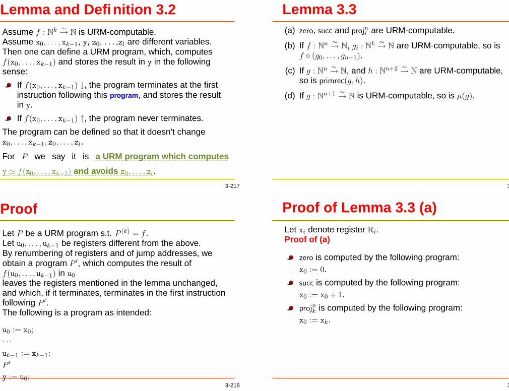
Lemma and Definition 3.2Assume f : Nk ∼→ N is URM-computable.Assume x0, . . . , xk−1, y, z0, . . . ,zl are different variables.Then one can define a URM program, which, computesf(x0, . . . , xk−1) and stores the result in y in the followingsense:

If f(x0, . . . , xk−1) ↓, the program terminates at the firstinstruction following this program, and stores the resultin y.

If f(x0, . . . , xk−1) ↑, the program never terminates.

The program can be defined so that it doesn’t changex0, . . . , xk−1, z0, . . . , zl.

For P we say it is::

a::::::

URM::::::::::::

program:::::::::

which:::::::::::::

computes

::::::::::::::::::::::

y ' f(x0, . . . , xk−1):::::

and:::::::::

avoids:::::::::::

z0, . . . , zl.

3-217

Proof

Let P be a URM program s.t. P (k) = f .Let u0, . . . , uk−1 be registers different from the above.By renumbering of registers and of jump addresses, weobtain a program P ′, which computes the result off(u0, . . . , uk−1) in u0

leaves the registers mentioned in the lemma unchanged,and which, if it terminates, terminates in the first instructionfollowing P ′.The following is a program as intended:

u0 := x0;

· · ·uk−1 := xk−1;

P ′

y := u0;3-218

Lemma 3.3(a) zero, succ and projni are URM-computable.

(b) If f : Nn ∼→ N, gi : Nk ∼→ N are URM-computable, so isf ◦ (g0, . . . , gn−1).

(c) If g : Nn ∼→ N, and h : Nn+2 ∼→ N are URM-computable,so is primrec(g, h).

(d) If g : Nn+1 ∼→ N is URM-computable, so is µ(g).

3-219

Proof of Lemma 3.3 (a)Let xi denote register Ri.Proof of (a)

zero is computed by the following program:x0 := 0.

succ is computed by the following program:x0 := x0 + 1.

projnk is computed by the following program:x0 := xk.

3-220


Assume f : Nn ∼→ N, gi : Nk ∼→ N are URM-computable.Show f ◦ (g0, . . . , gn−1) is computable.A plan for the program is as follows:

Input is stored in registers x0, . . . , xk−1.Let ~x := x0, . . . , xk−1.

First we compute gi(~x) for i = 0, . . . , k − 1, store result inregisters yi.

Then compute f(y0, . . . , yn−1),(which is ' f(g0(~x), . . . , gn−1(~x))),and store result in x0.

3-221

Proof of Lemma 3.3 (b)Problem: Computation of yi ' gi(~x)

might change ~x, which is used by later computations ofyj ' gj(~x) for j > i,

might change yj for j < i, which contains the result fromprevious computations of gj(~x).

By Lemma 3.2 possible to define programs as follows:

Let Pi be a URM program (i = 0, . . . , n − 1), whichcomputes yi ' gi(~x) and avoids yj for j 6= i.

Let Q be a URM program, which computesx0 ' f(y0, . . . , yn−1).

3-222

Proof of Lemma 3.3 (b)Let R be defined as follows:P0

· · ·Pn−1

Q

We show R(n)(~x) ' (f ◦ (g0(~x), . . . , gn−1(~x))).

3-223

Proof of Lemma 3.3 (b)R is the programP0

· · ·Pn−1

Q

Case 1: For one i gi(~x) ↑.The program will loop in program Pi for the first such i.R(n)(~x) ↑, f ◦ (g0, . . . , gn−1)(~x) ↑.

Case 2: For all i gi(~x) ↓.The program executes Pi, sets yi ' gi(x0, . . . , xk−1) andreaches beginning of Q.

3-224

Proof of Lemma 3.3 (b)R is the programP0

· · ·Pn−1

Q

Case 2.1: f(g0(~x), . . . , gn−1(~x)) ↑.Q will loop, R(n)(~x) ↑, f ◦ (g0, . . . , gn−1)(~x) ↑.Case 2.2: Otherwise.The program reaches the end of program Q andresult in x0 ' f(g0(~x), . . . , gn−1(~x)).So R(n)(~x) ' (f ◦ (g0, . . . , gn−1))(~x).

3-225

Proof of Lemma 3.3 (b)In all cases

R(n)(~x) ' (f ◦ (g0, . . . , gn−1))(~x) .

3-226

Proof of Lemma 3.3 (c)

Assume g : Nn ∼→ N, h : Nn+2 ∼→ N are URM-computable.Let f := primrec(g, h). Show f is URM-computable.Defining equations for f are as follows(let ~n := n0, . . . , nn−1):

f(~n, 0) ' g(~n),

f(~n, k + 1) ' h(~n, k, f(~n, k)).

3-227

Proof of Lemma 3.3 (c)Computation of f(~n, l) for l > 0 is as follows:

Compute f(~n, 0) as g(~n).

Compute f(~n, 1) as h(~n, 0, f(~n, 0)), using the previousresult.

Compute f(~n, 2) as h(~n, 1, f(~n, 1)), using the previousresult.

· · ·Compute f(~n, l) as h(~n, l − 1, f(~n, l − 1)), using theprevious result.

3-228

Proof of Lemma 3.3 (c)Plan for the program:

Let ~x := x0, . . . , xn−1.Let y, z, u be new registers.

Compute f(~x, y) for y = 0, 1, 2, . . . , xn, and store result inz.

Initially we have y = 0 (holds for all registers exceptof x0, . . . , xn initially).We compute z ' g(~x) (' f(~x, 0)).Then y = 0, z ' f(~x, 0).

3-229

Proof of Lemma 3.3 (c)

In step from y to y + 1:Assume that we have z ' f(~x, y).We want that after increasing y by 1 the::::::

loop::::::::::::

invariant z ' f(~x, y) still holds.Obtained as followsCompute u ' h(~x, y, z)(' h(~x, y, f(~x, y)) ' f(~x, y + 1)).Execute z := u (' f(~x, y + 1)).Execute y := y + 1.At the end , z ' f(~x, y) for the new value of y.

Iterate this as long as y 6= xn.Once y has reached xn, z contains f(~x, y) ' f(~x, xn).Execute x0 := z.

3-230

Proof of Lemma 3.3 (c)Let

P be a URM program, which computes z ' g(~x), andavoids y.

Q be a program, which computes u ' h(~x, y, z).

Let R be as follows:

P % Compute u ' g(~x, y, z)

while xn 6= y do {Q % Compute u ' h(~x, y, z)

% will be ' h(~x, y, f(~x, y)) ' f(~x, y + 1)

z := u;

y := y + 1; };x0 := z;

3-231

Proof of Lemma 3.3 (c)Correctness of this program:

When P is terminated, we have y = 0 andz ' g(~x) ' f(~x, y).

After each iteration of the while loop, we have y := y′ + 1and z ' h(~x, y′, z′).(y′, z′ are the previous values of y, z, respectively.)

Therefore we have z ' f(~x, y).

The loop terminates, when y has reached xn.Then z contains f(~x, y).This is stored in x0.

3-232

Proof of Lemma 3.3 (c)If P loops for ever, or in one of the iterations Q loops forever, then:

R loops, R(n+1)(~x, xn) ↑.f(~x, k) ↑ for some k < xn,subsequently f(~x, l) is undefined for all l > k.Especially, f(~x, xn) ↑.

Therefore f(~x, xn) ' R(n+1)(~x, xn).

3-233

Proof of Lemma 3.3 (d)

Assume g : Nn+1 ∼→ N is URM-computable.Show µ(g) is URM-computable as well.Note µ(g)(x0, . . . , xk−1) is the minimal z s.t.g(x0, . . . , xk−1, z) ' 0.Let ~x := x0, . . . , xk−1 and let y, z be registers different from ~x.

3-234

Proof of Lemma 3.3 (d)Plan for the program:

Compute g(~x, 0), g(~x, 1) , . . . until we find a k s.t.g(~x, k) ' 0.Then return k.

This is carried out by executing z ' g(~x, y) andsuccessively increasing y by 1 until we have z = 0.

Since we haven’t introduced a repeat-until-loop, wereplace this by a while loop as follows:

Initially we set z to something not 0.As long as z 6= 0, compute z ' g(~x, y) and thenincrease y by 1.If the while-loop terminates, we have y = n + 1 forthe minimal n s.t. g(~x, n) ' 0.Decrease y once, and store result in x0.

3-235

Proof of Lemma 3.3 (d)Let P compute z ' g(x0, . . . , xk−1, y).Let R be as follows:z := z + 1;

while z 6= 0 do {P

y := y + 1; };y := y−· 1;

x0 := y;

3-236

Proof of Lemma 3.3 (d)

R is z := z + 1;

while z 6= 0 do {P

y := y + 1; };y := y−· 1;

x0 := y;

z := 1 guarantees execution of the while loop at least once.Initially y = 0.After each iteration of the while loop, we have y := y′ + 1and z ' g(x0, . . . , xk−1, y

′), (y′ is the value of y before thisiteration).If loop terminates, we have z ' 0 and y = y′ + 1 for the

first value, such that g(x0, . . . , xk−1, y′) ' 0. x0 is then set to

that value. 3-237

Undecidability of the Halting ProblemUndecidability of the Halting Problem first proved 1936by Alan Turing.

We present this in context of URMs.

In the following “computable” means“URM-computable”.

Justified later by the Church-Turing-thesis.

3-238

Definition 3.4(a) A

:::::::::::

problem is an n-ary predicate M(x0, . . . , xn−1) ofnatural numbers, i.e. a property of n-tuples of naturalnumbers.

(b) A problem M is::::::::::::

decidable, if the characteristic functionof M defined by

χM (x0, . . . , xn−1) :=

{1 if M(x0, . . . , xn−1) holds,0 otherwise

is computable.

3-239

Example of ProblemsThe binary predicate

Multiple(x, y) :⇔ x is a multiple of y

is a problem.

χM (x0, . . . , xn−1) decides, whether M(x0, . . . , xn−1)holds (then it returns 1 for yes), or not.

χMultiple(x, y) =

{1 if x is a multiple of y,0 if x is not a multiple of y.

χMultiple is intuitively computable, therefore Multiple isdecidable.

3-240

URM programsURM-programs can be written as a string ofASCII-symbols.

→ URM programs elements of A∗, whereA = set of ASCII-symbols.

→ URM programs can be encoded as natural numbers.Let for a URM program P , code(P ) ∈ N be its code.

It is intuitively decidable, whether a string of ASCIIsymbols is a URM-program.

One can show that this can be decided by a URM.

→ It is intuitively decidable, whether n = code(P ) for aURM-program P .

However, the halting problem is undecidable.

3-241

Definition 3.5The

:::::::::

Halting::::::::::::

Problem is the following binary predicate:

Halt(x, y) :⇔

1 if x = code(P ) for a URM program P

and P (1)(y) ↓0 otherwise

3-242

ExampleLet P be a code for the URM programifzero(0, 0)

If input is > 0, the program terminates immediately, and R0

remains unchanged, so P (0)(k) ' k for k > 0.If input is = 0, the program loops for ever.Therefore P (0)(0) ↑.Let e = code(P ). Then Halt(e, n) holds for n > 0 and doesnot hold for n = 0.

3-243

RemarkBelow we will see: Halt is undecideable.

However, WeakHalt is computable:

WeakHalt(x, y) :'

1 if x = code(P )

for a URM program P

and P (1)(y) ↓undefined otherwise

Computed as follows:First check whether x = code(P ) for some URMprogram P .If not, enter an infinite loop.Otherwise, simulate P with input y.If simulation stops, output 1, otherwise the programloops for ever.

3-244

Theorem 3.6Theorem 3.6 The halting problem is undecidable.

Proof:Assume P (2) decides the Halting Problem, i.e.

P (2)(x, y) '{

1 if x codes a URM program Q s.t. Q(1)(y) ↓0 otherwise.

We define a computable function f : N∼→ N, which cannot

be computed by the URM with code e, as violated on inpute.

We argue similar to the proof that N 6' P(N):

3-245

Proof of Theorem 3.6

P (2)(x, y) '{


If P (2)(e, e) ' 1, i.e. e encodes a URM Q and Q(1)(e) ↓, thenlet f(e) ↑.

Therefore, Q(1) 6= f .

3-246


P (2)(x, y) '{


If P (2)(e, e) ' 0, i.e. e doesn’t encode a URM, or it encodesa URM Q and Q(1)(e) ↑, then we let f(e) ↓: f(e) :' 0.Therefore, if e encodes a URM Q, we have Q(1) 6= f .The complete definition is as follows:

f(e) '{

0 if P (2)(e, e) ' 0

undefined otherwise.

f is not URM-computable: f = R(1) is violated at input

code(R):3-247


P (2)(x, y) '{


f(e) '{

0 if P (2)(e, e) ' 0


Assume f = R(1). Then

R(1)(code(R)) ↓ property of P⇔ P (2)(code(R), code(R)) ' 1

Def of f⇔ f(code(R)) ↑f=R(1)

⇔ R(1)(code(R)) ↑

3-248


P (2)(x, y) '{


f(e) '{

0 if P (2)(e, e) ' 0


Therefore, f 6= R(1), f cannot be computed by any URMprogram R. However, f can be intuitively computed, (theprogram makes use of P ).It can be shown that it is in fact URM-computable.So we get a contradiction.

3-249

RemarkThe above proof can easily be adapted to anyreasonable programming language, in which one candefine all computable functions.

Such programming languages are called:::::::::::::::::::::

Turing-complete languages.Babbage’s machine was, if one removes therestriction to finite memory, Turing-complete, since ithad a conditional jump.

For standard Turing complete languages, theunsolvability of the Turing-halting problem means:it is not possible to write a program, which checks,whether a program on given input terminates.

3-250

Sec. 4: Turing MachinesThere are two problems with the model of a URM:

Execution of a single URM instruction might takearbitrarily long:

Consider succ(n).If Rn contains in binary 111 · · · 111︸︷︷︸

k times

, this instruction

replaces it by 1 000 · · · 000︸︷︷︸k times

.

We have to replace k symbols 1 by 0.k is arbitrary→ this single step might take arbitrarily long time.

4-251

First Problem of URMsTherefore URMs unsuitable as a basis for defining thecomplexity of algorithms.

However, there are theorems linking complexity ofURMs to actual complexities of algorithms.

4-252

Second Problem of URMsWe aim at a notion of computability, which covers allpossible ways of computing something, independentlyof any concrete machine.

URMs are a model of computation which covers currentstandard computers.

However, there might be completely different notions ofcomputability, based on symbolic manipulations of asequence of characters, where it might be morecomplicated to see directly that all such computationscan be simulated by a URM.

It is more easy to see that such notions are covered bythe Turing machine model of computation.

4-253

Idea of a Turing MachineIdea of a Turing machine (

::::

TM):Analysis of a computation carried out by a human being(:::::::

agent) on a piece of paper.

15 . 16=

15

90

240

4-254

Idea of a Turing MachineSteps in this formulation:

Algorithm should be deterministic.→ The agent will use only finitely many symbols, putat discrete positions on the paper.

1 5 . 1 6 =

1 5

9 0

− − −2 4 0

4-255

Idea of a Turing MachineWe can replace a two-dimensional piece of paper byone potentially infinite tape, by using a specialsymbol for a line break.Each entry on this tape is called a

:::::

cell:

· · · 1 5 . 1 6 = CR 1 5 CR · · ·

4-256

Steps in Formulising TMsIn the real situation, agent can look at several cells atthe same time,but bounded by his physical capability.Can be simulated by looking at one cell only at anytime, and moving around in order to get informationabout neighbouring cells.

· · · 1 5 . 1 6 = CR 1 5 CR · · ·↑

Head

4-257

Steps in Formulising TMsIn the real situation, an agent can make arbitraryjumps, but bounded by the physical ability of theagent.Each such jump can be simulated by finitely manyone-step jumps.→ Restriction to one-step movements.

· · · 1 5 . 1 6 = CR 1 5 CR · · ·↑

Head

4-258

Steps in Formulising TMsAgent operates purely mechanistically:Reads a symbol, and depending on it changes it andmakes a movement.Agent himself will have only finite memory.→ There is a finite state of the agent, and, dependingon the state and the symbol at the head, a nextstate, a new symbol, and a movement is chosen.

· · · 1 3 . 3 7 = CR 1 5 CR · · ·↑s0

4-259

Definition of TMs· · · 1 5 . 1 6 = CR 1 5 CR · · ·

↑s0

A::::::::

Turing::::::::::::

machine is a quintuple (Σ, S, I, xy, s0), whereΣ is a finite set of symbols, called the

:::::::::::

alphabet ofthe Turing machine. On the tape, the symbols in Σwill be written.S is a finite set of states.

4-260

Definition of TMs· · · 1 5 . 1 6 = CR 1 5 CR · · ·

↑s0

I is a finite sets of quintuples (s, a, s′, a′, D), wheres, s′ ∈ S,a, a′ ∈ ΣD ∈ {L,R},

s.t. for every s ∈ S, a ∈ Σ there is at most one s′, a′, Ds.t. (s, a, s′, a′, D) ∈ S.The elements of I are called

:::::::::::::::

instructions.

xy ∈ Σ (a symbol for blank).

s0 ∈ S (the initial state).

4-261

Meaning of InstructionsA instruction (s, a, s′, a′, D) ∈ I means the following:

If the Turing machine is in state s, and the symbol atposition of the head is a, then

the state is changed to s′,the symbol at this position is changed to a′,if D = L, the head moves left,if D = R, the head moves right.

Example:(s0, 1, s1, 0,R)(s1, 6, s2, 7, L)

· · · 1 5 . 0 7 = CR 1 5 CR · · ·↑s2

4-262

Meaning of InstructionsIf the Turing machine is in a state s and reads symbol aat his head, and there are no s′, a′, D s.t.(s, a, s′, a′, D) ∈ I, then the Turing machine stops.

4-263

Example of a TMDevelopment of a TM with Σ = {0, 1, xy},

where xy is the symbol for the blank entry.

Functionality of the TM:Assume initially

Tape contains binary number,Rest of the tape contains xy.Head points to any digit of the number.TM in state s0.

Then the TM stops after finitely many steps and thenthe tape contains the original number incrementedby one,the rest of tape contains xy,the head points to most significand bit.

4-264

ExampleInitially

· · · 1 0 1 0 0 1 0 0 1 1 1 · · ·↑s0

Finally

· · · 1 0 1 0 0 1 0 1 0 0 0 · · ·↑s3

4-265

Construction of the TMTM is ({0, 1, xy}, S, I, xy, s0).

States S and instructions I developed in the following.

4-266

Step 1Initially, move head to least significant bit.

I.e. as long as symbol at head is 0 or 1, move right,leave symbol as it is.If symbol is xy, move head left, leave symbol againas it is.

Achieved by the following instructions:(s0, 0, s0, 0,R)

(s0, 1, s0, 1,R)

(s0, xy, s1, xy, L).

At the end TM is in state s1.

· · · 1 0 1 0 0 1 0 0 1 1 1 · · ·↑s0

4-267

Step 1Initially, move head to least significant bit.

I.e. as long as symbol at head is 0 or 1, move right,leave symbol as it is.If symbol is xy, move head left, leave symbol againas it is.

Achieved by the following instructions:(s0, 0, s0, 0,R)

(s0, 1, s0, 1,R)

(s0, xy, s1, xy, L).

At the end TM is in state s1.

· · · 1 0 1 0 0 1 0 0 1 1 1 · · ·↑s1

4-267

Step 2Increasing a binary number b done as follows:

Case number consists of 1 only:I.e. b = (111 · · · 111︸︷︷︸

k times

)2.

b + 1 = (1 000 · · · 000︸︷︷︸k times

)2.

Obtained by replacing all ones by zeros and thenreplacing the first blank symbol by 1.

4-268

Step 2Otherwise:

Then the representation of the number contains atthe end one 0 followed by ones only.Includes case where the least significant digit is 0.

Example 1: b = (0100010111)2, one 0 followed by 3ones.Example 2: b = (0100010010)2, least significantdigit is 0.

Let b = (b0b1 · · · bk0 111 · · · 111︸︷︷︸l times

)2.

b + 1 obtained by replacing the final block of ones by0 and the 0 by 1:b + 1 = (b0b1 · · · bk1 000 · · · 000︸︷︷︸

l times

)2.

4-269

General SituationWe have to replace, as long as we find ones, the onesby zeros, and move left, until we encounter a 0 or a xy,which is replaced by a 1.

So we have the new state s2, and the followinginstructions:

(s1, 1, s1, 0, L).(s1, 0, s2, 1, L).(s1, xy, s2, 1, L).

At the end the head will be one field to the left of the 1written, and the state will be s2.

· · · 1 0 1 0 0 1 0 1 0 0 0 · · ·↑s2

4-270

Step 3Finally, we have to move the most significant bit, which isdone as follows:

(s2, 0, s2, 0, L).

(s2, 1, s2, 1, L).

(s2, xy, s3, xy,R).

The program terminates in state s3.

· · · 1 0 1 0 0 1 0 1 0 0 0 · · ·↑s3

4-271

Complete ProgramThe complete TM is as follows:

({0, 1, xy},{s0, s1, s2, s3},{(s0, 0, s0, 0,R),

(s0, 1, s0, 1,R),

(s0, xy, s1, xy, L),

(s1, 1, s1, 0, L),

(s1, 0, s2, 1, L),

(s1, xy, s2, 1, L),

(s2, 0, s2, 0, L),

(s2, 1, s2, 1, L),

(s2, xy, s3, xy,R)}, s0, xy)

4-272

Definition 4.1Let M = (Σ, S, I, xy, s0) be a Turing machine with {0, 1} ⊆ Σ.Define for every k ∈ N M (k)

:::::: Nk ∼→ N, where

M (k)(a0, . . . , ak−1) is computed as follows:

Initialisation:The head is an arbitrary position.Starting from this, we writebin(a0)xybin(a1)xy · · · xybin(ak−1) on the tape, wherebin(a) is the binary string corresponding to a.

E.g. if k = 3, a0 = 0, a1 = 3, a2 = 2 then we write0xy11xy10.

All other cells contain xy.The state is set to s0.

Iteration: Run the TM, until it stops.4-273

Definition 4.1Output:

Case 1: The TM stops.Only finitely many cells are non-blank.Let tape, starting from the head-position, containb0b1 · · · bk−1c where bi ∈ {0, 1} and c 6∈ {0, 1}.(k might be 0).Let a = (b0, . . . , bk−1)2 (in case k = 0, a = 0).Then M (k)(a0, . . . , ak−1) ' a.

4-274

Definition 4.1Example: Let Σ = {0, 1, a, b, xy}.

If tape contains· 01010xy0101xy· or 01010axy,output is (01010)2 = 10.If tape contains at the end· abxy· or a,· or xy,the output is 0.

Case 2: Otherwise.Then M (k)(a0, . . . , ak−1) ↑.

4-275

Definition 4.2f : Nk ∼→ N is

::::::::::::::::::::::::

Turing-computable, in short

::::::::::::::::::::

TM-computable, if f = M (k) for some TM M , the alphabetof which contains {0, 1}.

Example: That succ : N∼→ N is Turing-computable was

shown above.

4-276

Theorem 4.3If f : Nn ∼→ N is URM-computable, then it is as well Turing-

computable by a TM with alphabet {0, 1, xy}.

4-277

Proof of Theorem 4.3Notation:::::

The::::::

tape:::

of:::

a::::

TM::::::::::::

contains:::::::::::

a0, . . . , al means:

Starting from the head position, the cells of the tapecontain a0, . . . , al.

All other cells contain xy.

Furthermore, in this proof, bin(n) will stand for any binaryrepresentation of n.

E.g. bin(2) could be any of 10, 010, 0010 etc.

4-278

Proof of Theorem 4.3Assume

f = P (n),

P refers only to R0, . . . ,Rl−1 and l > n,

We define a TM M , which simulates P . Done as follows:

That the registers R0, . . . ,Rl−1 contain a0, . . . , al−1 issimulated by the tape containing bin(a0)xy · · · xybin(al−1).

An instruction Ij will be simulated by states qj,0, . . . , qj,i

with instructions for those states.

4-279

Conditions on the SimulationAssume the URM P is in a state s.t.

R0, . . . ,Rl−1 contain a0, . . . , al−1,the URM is about to execute Ij.

Assume after executing Ij , the URM is in a state whereR0, . . . ,Rl−1 contain b0, . . . , bl−1,the PC contains k.

Then we want that, if configuration of the TM M is, s.t.the tape contains bin(a0)xybin(a1)xy · · · xybin(al−1),and the TM is in state qj,0,

then the TM reaches a configuration s.t.the tape contains bin(b0)xybin(b1)xy · · · xybin(bl−1),the TM is in state qk,0.

4-280

ExampleAssume the URM is about to execute instruction

I4 = pred(0) (i.e. PC = 4),with register contentsR0 R1 R2

2 1 3

Then the URM will end withPC = 5and register contentsR0 R1 R2

2 1 2

4-281

ExampleThen we want that, if the simulating TM is

in state q4,0,with tape content bin(2)xybin(1)xybin(3)

it should reachstate q5,0

with tape content bin(2)xybin(1)xybin(2)

4-282

Proof of Theorem 4.3Furthermore, we need initial states qinit,0, . . . , qinit,j andcorresponding instructions, s.t.

if the TM initiallybin(b0)xybin(b1)xy · · · xybin(bn−1),it will reach state q0,0 with the tape containingbin(b0)xybin(b1)xy · · · xybin(bn−1)xy 0xy0xy · · · xy0︸︷︷︸

l − n times

xy.

4-283

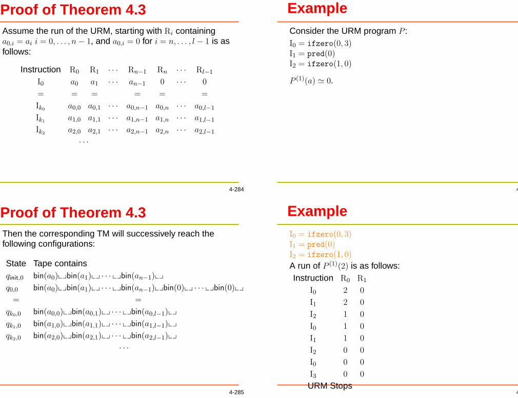
Proof of Theorem 4.3Assume the run of the URM, starting with Ri containinga0,i = ai i = 0, . . . , n − 1, and a0,i = 0 for i = n, . . . , l − 1 is asfollows:

Instruction R0 R1 · · · Rn−1 Rn · · · Rl−1

I0 a0 a1 · · · an−1 0 · · · 0

= = = = = =

Ik0a0,0 a0,1 · · · a0,n−1 a0,n · · · a0,l−1

Ik1a1,0 a1,1 · · · a1,n−1 a1,n · · · a1,l−1

Ik2a2,0 a2,1 · · · a2,n−1 a2,n · · · a2,l−1

· · ·

4-284

Proof of Theorem 4.3Then the corresponding TM will successively reach thefollowing configurations:

State Tape containsqinit,0 bin(a0)xybin(a1)xy · · · xybin(an−1)xy

q0,0 bin(a0)xybin(a1)xy · · · xybin(an−1)xybin(0)xy · · · xybin(0)xy

= =

qk0,0 bin(a0,0)xybin(a0,1)xy · · · xybin(a0,l−1)xy



· · ·

4-285

ExampleConsider the URM program P :I0 = ifzero(0, 3)I1 = pred(0)I2 = ifzero(1, 0)

P (1)(a) ' 0.

4-286

ExampleI0 = ifzero(0, 3)I1 = pred(0)I2 = ifzero(1, 0)

A run of P (1)(2) is as follows:Instruction R0 R1

I0 2 0

I1 2 0

I2 1 0

I0 1 0

I1 1 0

I2 0 0

I0 0 0

I3 0 0

URM Stops4-287

Corresponding TM SimulationI0 = ifzero(0, 3)I1 = pred(0)I2 = ifzero(1, 0)

Instruction R0 R1 State of TM Content of Tapeqinit,0 bin(2)xy

I0 2 0 q0,0 bin(2)xybin(0)xy








URM Stops TM Stops4-288

Proof of Theorem 4.3If we have defined this we have

If Pn(a0, . . . , an−1) ↓, Pn(a0, . . . , an−1) ' j, then Peventually stops with Ri containing some values bi,where b0 = j.Then, the TM M starting with bin(a0)xy · · · xybin(an−1)will eventually terminate in a configurationbin(b0)xy · · · xybin(bn−1).Therefore Mn(a0, . . . , an−1) ' b0 = j.

If Pn(a0, . . . , an−1) ↑, the URM P will loop and the TM Mwill carry out the same steps as the URM and loop aswell.Therefore Mn(a0, . . . , an−1) ↑,again Pn(a0, . . . , an−1) ' Mn(a0, . . . , an−1).

It follows P (n) = M (n), and the proof is complete, if thesimulation has been introduced.

4-289

Proof of Theorem 4.3Informal description of the simulation of URM instructions.

Initialisation.Initially, the tape contains bin(a0)xy · · · xybin(an−1).We need to obtain configuration:bin(a0)xy · · · xybin(an−1)xy bin(0)xy · · · xybin(0)︸︷︷︸

l − n times

.

Achieved bymoving head to the end of the initial configurationinserting, starting from the next blank, l − n-times0xy,then moving back to the beginning.

4-290

Proof of Theorem 4.3Simulation of URM instructions.

Simulation of instruction Ik = succ(j).Need to increase (j + 1)st binary number by 1 Initialconfiguration:

bin(c0) xy bin(c1) xy · · · xy bin(cj) xy · · · xy bin(cl) xy

↑qk,0

First move to the (j + 1)st blank to the right. Then weare at the end of the (j + 1)st binary number.


↑

4-291



↑

Now perform the operation for increasing by 1 asabove.At the end we obtain:

bin(c0) xy bin(c1) xy · · · xy bin(cj + 1) xy · · · xy bin(cl) xy

↑It might be that we needed to write over theseparating blank a 1, in which case we have:

bin(c0) xy bin(c1) xy · · · bin(cj−1) bin(cj + 1) xy · · · xy bin(cl) xy

↑4-292

Proof of Theorem 4.3In the latter case, shift all symbols to the left once left, inorder to obtain a separating xy between the lth andl − 1st entry.We obtain

bin(c0) xy bin(c1) xy · · · bin(cj−1) xy bin(cj + 1) xy · · · xy bin(cl) xy

↑Otherwise, move the head to the left, until we reach the(j + 1)st blank to the left, and then move it once to theright.We obtain

bin(c0) xy bin(c1) xy · · · xy bin(cj + 1) xy · · · xy bin(cl) xy

↑

4-293

Proof of Theorem 4.3Simulation of instruction Ik = pred(j).

Assume the configuration at the beginning is :

bin(c0) xy bin(c1) xy · · · bin(cj) xy · · · xy bin(cl) xy

↑

We want to achieve

bin(c0) xy bin(c1) xy · · · bin(cj−· 1) xy · · · xy bin(cl) xy

↑

Done as follows:

4-294

Proof of Theorem 4.3Initially: bin(c0) xy · · · xy bin(cj) xy · · · xy bin(cl) xy

↑Finally: bin(c0) xy · · · xy bin(cj−· 1) xy · · · xy bin(cl) xy

↑

Move to end of the (j + 1)st number.Check, if the number consists only of zeros or not.

If it consists only of zeros, pred(j) doesn’t changeanything.Otherwise, number is of the form b0 · · · bk1 00 · · · 0︸︷︷︸

l′ times

.

Replace it by b0 · · · bk0 11 · · · 1︸︷︷︸l′ times

.

Done as for succ.

4-295

Proof of Theorem 4.3Initially: bin(c0) xy · · · xy bin(cj) xy · · · xy bin(cl) xy

↑Finally: bin(c0) xy · · · xy bin(cj−· 1) xy · · · xy bin(cl) xy

↑

We have achieved


↑Move back to the beginning:


↑

4-296

Proof of Theorem 4.3Simulation of instruction Ik = ifzero(j, k′).

Move to j + 1st binary number on the tape.Check whether it contains only zeros.

If yes, switch to state qk′,0.Otherwise switch to state qk+1,0.

This completes the simulation of the URM P .

4-297

RemarkWe will later show that TM-computable impliesURM-computable

Done by showingTM-computable imlies partial recursive,partial recursive implies URM-computable

This is more convenient.

Therefore the TM and URM model of computationcoincide.

4-298

Extension to Arbitrary AlphabetsLet A be a finite alphabet s.t. xy 6∈ A, and B := A∗.

To a Turing machine T = (Σ, S, I, xy, s0) with A ⊆ Σ

corresponds a partial function T (A,n) : Bn ∼→ B, whereT (A,n)(a0, . . . , an−1) is computed as follows:

Initially write a0xy · · · xyan−1 on the tape, otherwisexy.Start in state s0 on the left most position of a0.Iterate TM as before.In case of termination, the output of the function isc0 · · · cl−1, if the tape contains, starting with the headposition c0 · · · cl−1d with ci ∈ A, d 6∈ A.Otherwise, the function value is undefined.

4-299

Extension to Arbitrary AlphabetsNotion is modulo encoding of A∗ into N equivalent to thenotion of Turing-computability on N.

However, when considering complexity bounds, thisnotation might be more appropriate.

Avoids encoding/decoding into N.

4-300

Turing-computable predicatesA predicate A is Turing-decidable, iff χA isTuring-computable.

Instead of simulating χA

means to write the output of χA (a binary number 0or 1) on the tape

it is more convenient, to take TM with two additionalspecial states strue and sfalse corresponding to truth andfalsity of the predicate.

4-301

Turing-computable predicatesThen a predicate is Turing decidable, if, when we writeinitially the inputs as before on the tape and startexecuting the TM,

it always terminates in strue or sfalse,and it terminates in strue, iff the predicate holds forthe inputs,and in sfalse, otherwise.

Notion is equivalent to the first notion.

Usually taken as basis for complexity considerations.

4-302

5. Algebraic View of ComputabilityURM and TM based on universal programminglanguages.

Next model: Functions generated frombasic functionsby using certain operations.

First proposed by Gödel and Kleene 1936.

Best model for showing that functions are computable.

5-303

Overview1. Introduction of primitive-recursive functions.

Will be total.Includes all functions which can be computedrealistically, and many more.But not all computable functions are primitiverecursive.

2. Introduction of the partial recursive functions.Complete model of computation.

3. Proof that sets of URM-computable functions, ofTM-computable functions and of partial-recursivefunctions coincide.

5-304

Def. Prim.-Rec. FunctionsInductive definition of the

::::::::::::::::::::::::

primitive-recursive functionsf : Nk → N.

The following:::::::

basic::::::::::::::

Functions are primitive recursive:

zero : N → N,succ : N → N,

projki : Nn → N (0 ≤ i ≤ k).

Remember that these functions have defining equationszero(n) = 0,succ(n) = n + 1,

projki (a0, . . . , ak−1) = ai.

5-305

Def. Prim.-Rec. FunctionsIf

f : Nk → N is primitive-recursive,gi : Nn → N are primitive-recursive, (i = 0, . . . , k − 1),

so is f ◦ (g0, . . . , gk−1) : Nn → N.

Remember that h := f ◦ (g0, . . . , gk−1) is defined ash(~x) = f(g0(~x), . . . , gk−1(~x)).

Notations:In case k = 1, write f ◦ g instead of f ◦ (g).Write f0 ◦ f1 ◦ f2 ◦ · · · ◦ fn instead off0 ◦ (f1 ◦ (f2 ◦ · · · ◦ fn)).

5-306


g : Nn → N,h : Nn+2 → N are primitive-recursive,

so is primrec(g, h) : Nn+1 → N.

Remember that f := primrec(g, h) is defined byf(~x, 0) = g(~x),f(~x, n + 1) = h(~x, n, f(~x, n)).

5-307


k ∈ N,h : N2 → N is primitive-recursive,

so is primrec(k, h) : N → N.

Remember that f := primrec(k, h) is defined byf(0) = k,f(n + 1) = h(n, f(n)).

5-308

Inductively Defined SetsThat the set of primitive recursive functions is inductivelydefined means:

It is the least setcontaining basic functionsand closed under the operations.

Or: It is the set generated by the above.

Or: The primitive recursive functions are those we canwrite as terms formed

from zero, succ, projni ,using composition _ ◦ (_, . . . , _)

i.e. by forming from f, gi f ◦ (g0, . . . , gn−1)

and primrec.

5-309

Inductively Defined SetsE.g.

primrec(proj10︸︷︷︸:N→N

, succ︸︷︷︸:N→N

◦ proj32︸︷︷︸:N3→N︸︷︷︸

:N3→N

)

︸︷︷︸:N2→N

: N2 → N is prim. rec.

(= addition)

primrec( 0︸︷︷︸∈N

, proj20︸︷︷︸:N2→N

)

︸︷︷︸:N1→N

: N → N is prim. rec.

(= pred)

5-310

Primitive-Rec. RelationsA relation R ⊆ Nn is

::::::::::::::::::::::::

primitive-recursive, if

χR : Nn → N

is primitive-recursive.

5-311

Identity Functionid : N → N, id(n) = n is primitive-recursive:

id = proj10:proj10 : N1 → N,proj10(n) = n = id(n).

5-312

Constant Functionconstn : N → N, constn(k) = n is primitive-recursive:constn = succ ◦ · · · ◦ succ︸︷︷︸

n times

◦zero:

succ ◦ · · · ◦ succ︸︷︷︸n times

◦zero(k) = succ(succ(· · · succ︸︷︷︸n times

(zero(k))))

= succ(succ(· · · succ(︸︷︷︸n times

0)))

= 0 +1 + 1 · · · + 1︸︷︷︸n times

= n

= constn(k) .

5-313

Additionadd : N2 → N, add(x, y) = x + yis primitive-recursive.We have the laws:

add(x, 0) = x + 0

= x

add(x, y + 1) = x + (y + 1)

= (x + y) + 1

= add(x, y) + 1

5-314

Addition

add(x, 0) = x + 0 ,

add(x, y + 1) = add(x, y) + 1 .

add(x, 0) = g(x),whereg : N → N, g(x) = x,i.e. g = id = proj10.

5-315

Addition

add(x, 0) = x + 0 = g(x) ,

add(x, y + 1) = add(x, y) + 1 .

add(x, y + 1) = h(x, y, add(x, y)),whereh : N3 → N, h(x, y, z) := z + 1.h = succ ◦ proj30:

(succ ◦ proj32)(x, y, z) = succ(proj32(x, y, z))

= succ(z)

= z + 1

= h(x, y, z) .

5-316

Addition

add(x, 0) = x + 0 = g(x) ,

add(x, y + 1) = add(x, y) + 1 = h(x, y, add(x, y)) ,

g = proj10 ,

h = succ ◦ proj32 .

Therefore

add = primrec(proj10, succ ◦ proj32) .

5-317

Multiplicationmult : N2 → N, mult(x, y) = x · yis primitive-recursive.We have the laws:

mult(x, 0) = x · 0 = 0

mult(x, y + 1) = x · (y + 1)

= x · y + x

= mult(x, y) + x

= add(mult(x, y), x)

5-318

Multiplication

mult(x, 0) = 0 ,

mult(x, y + 1) = add(mult(x, y), x) .

mult(x, 0) = g(x), where g : N → N, g(x) = 0,i.e. g = zero,

5-319

Multiplication

mult(x, 0) = 0 = g(x) ,

mult(x, y + 1) = add(mult(x, y), x) .

mult(x, y + 1) = h(x, y,mult(x, y)),whereh : N3 → N, h(x, y, z) := add(z, x).h = add ◦ (proj32, proj

30):

(add ◦ (proj32, proj30))(x, y, z) = add(proj32(x, y, z), proj30(x, y, z))

= add(z, x)

= h(x, y, z) .

5-320

Multiplication

mult(x, 0) = 0 = g(x) ,

mult(x, y + 1) = add(mult(x, y), x) = h(x, y,mult(x, y)) ,

g = zero ,

h = add ◦ (proj32, proj30) .

Therefore

mult = primrec(zero, add ◦ (proj32, proj30)) .

5-321

RemarkUnless demanded explicitly, for showing that f isdefined by primrec, it suffices to express:

f(~x, 0) as an expression built frompreviously defined prim.-rec. functions,~x,and constants.

Example:

f(x0, x1, 0) = (x0 + x1) · 3 .

5-322

Remarkf(~x, y + 1) as an expression built from

previously defined prim.-rec. functions,~x,the

::::::::::::

recursion:::::::::::::

argument y,the

::::::::::::

recursion:::::::::::::::

hypothesis f(~x, y),and constants.

Example:

f(x0, x1, y + 1) = (x0 + x1 + y + f(x0, x1, y)) · 3 .

5-323

RemarkSimilarly, for showing directly f is prim.-rec., it sufficesto express f(~x) in terms of

previously defined prim.-rec. functions,parameters ~x

constants.Example:

f(x, y, z) = (x + y) · 3 + z .

5-324

Predecessor Functionpred is prim.-rec.:

pred(0) = 0 ,

pred(x + 1) = x ,

5-325

Subtractionsub(x, y) = x−· y is prim.-rec.:

sub(x, 0) = x ,

sub(x, y + 1) = pred(sub(x, y)) .

5-326

Signum Functionsig : N → N,

sig(x) :=

{1, if x > 0,0, if x = 0

is prim.-rec.:sig(x) = x−· (x−· 1):

For x = 0 we have

x−· (x−· 1) = 0−· (0−· 1) = 0−· 0

= 0 = sig(x) .

For x > 0 we have

x−· (x−· 1) = x − (x − 1) = x − x + 1

= 1 = sig(x) .

5-327

x < y is Prim.-Rec.A(x, y) :⇔ x < y is primitive-recursive, sinceχA(x, y) = sig(y−· x):

If x < y, theny−· x = y − x > 0 ,

thereforesig(y−· x) = 1 = χA(x, y)

If ¬(x < y), i.e. x ≥ y,then

y−· x = 0 ,

sig(y−· x) = 0 = χA(x, y) .

5-328

Add., Mult., Exp.Consider the sequence of definitions of addition,multiplication, exponentiation:

Addition:

n + 0 = n ,

n + (m + 1) = (n + m) + 1 ,

Therefore, if we write (+1) for the function N → N,(+1)(n) = n + 1, then

n + m = (+1)m(n) .

5-329

Add., Mult., Exp.Multiplication:

n · 0 = 0 ,

n · (m + 1) = (n · m) + n ,

Therefore, if we write (+n) for the function N → N,(+n)(k) = k + n, then

n · m = (+n)m(0) .

5-330

Add., Mult., Exp.Exponentiation:

n0 = 1 ,

nm+1 = (nm) · n ,

Therefore, if we write (·n) for the function N → N,(·n)(m) = n · m, then

nm = (·n)m(1) .

5-331

SuperexponentiationExtend this sequence further, by defining

Superexponentiation:

superexp(n, 0) = 1 ,

superexp(n,m + 1) = nsuperexp(n,m) ,

Therefore, if we write (n ↑) for the function N → N,(n ↑)(k) = nk, then

nm = (n ↑)m(1) .

5-332

SupersuperexponentiationSupersuperexponentiation:

supersuperexp(n, 0) = 1 ,

supersuperexp(n,m + 1) = superexp(n, supersuperexp(n,m)) ,

Etc.

One obtains sequence of extremely fast growingfunctions.

Traditionally, instead of considering such binaryfunctions, one considers a sequence of unary functions.with similar growth rate.These functions are called the

:::::::::::::::

Ackermann:::::::::::::

functions.They exhaust all prim.-rec. functions.

5-333

The Ackermann FunctionLet n ∈ N.The

:::::

n-th::::::::::

branch:::

of:::::

the:::::::::::::::

Ackermann::::::::::::

functionAckn : N → N, is defined by

Ack0(y) = y + 1 ,

Ackn+1(y) = (Ackn)y+1(1) := Ackn(Ackn(· · ·Ackn(︸︷︷︸y + 1 times

1))) .

Ackn is prim.-rec. for fixed n.

5-334

The Ackermann Function

Ack0(y) = y + 1 ,

Ackn+1(y) = (Ackn)y+1(1) .

Proof that Ackn is prim.-rec. by Induction(n):

Base-case:Ack0 = succ is prim.-rec.

Induction step:Assume Ackn is primitive-recursive.Show Ackn+1 is primitive-recursive.We have:

Ackn+1(0) = Ackn(1) ,

Ackn+1(y + 1) = Ackn(Ackn+1(y)) .

5-335

The Ackermann FunctionTherefore Ackn+1 is primitive-recursive.

5-336

Remark on Ackermann Function

Ack0(n) = n + 1 .

Ack1(n) = Ackn+10 (1)

= 1 +1 + · · · + 1︸︷︷︸n + 1 times

= 1 + n + 1 = n + 2 .

Ack2(n) = Ackn+11 (1)

= 1 +2 + · · · + 2︸︷︷︸n + 1 times

= 1 + 2(n + 1)

= 2n + 3 > 2n .

5-337


Ack2(n) > 2n .

Ack3(n) = Ackn+12 (1)

> 2 · 2 · · · · · 2︸︷︷︸n + 1 times

·1

= 2n+1 > 2n .

Ack4(n) = Ackn+13 (1)

> 2···21

︸︷︷︸n + 1 times

.

5-338


Ack4(n) > 2···21

︸︷︷︸n + 1 times

.

Ack5(n) will iterate Ack4 n + 1 times, etc.

So for small n, Ack5(n) will exceed the number of particles

in the universe, and Ack5 is therefore not realistically com-

putable.

5-339

The Ackermann FunctionAckn for fixed n is primitive-recursive.

However, we will show below that a uniform version ofthe Ackermann function,i.e. Ack : N2 → N,

Ack : N2 → N ,

Ack(x, y) := Ackx(y) ,

is not primitive-recursive.

5-340

Closure under ∪, ∩, \If R,S ⊆ Nn are prim.-rec., so are

R ∪ S,R ∩ S,Nn \ R.

Note:(R ∪ S)(~x) ⇔ R(~x) ∨ S(~x),(R ∩ S)(~x) ⇔ R(~x) ∧ S(~x),(Nn \ R)(~x) ⇔ ¬R(~x).

5-341

Closure under ∪, ∩, \Proof of (R ∪ S)(~x) ⇔ R(~x) ∨ S(~x):

(R ∪ S)(~x) ⇔ ~x ∈ R ∪ S

⇔ ~x ∈ R ∨ ~x ∈ S

⇔ R(~x) ∨ S(~x)

Proof of (R ∩ S)(~x) ⇔ R(~x) ∧ S(~x):

(R ∩ S)(~x) ⇔ ~x ∈ R ∩ S

⇔ ~x ∈ R ∧ ~x ∈ S

⇔ R(~x) ∧ S(~x)

5-342

Closure under ∪, ∩, \Proof of (Nn \ R)(~x) ⇔ ¬R(~x):

(Nn \ R)(~x) ⇔ ~x ∈ (Nn \ R)

⇔ ~x 6∈ R

⇔ ¬R(~x)

5-343

Closure under ∪, ∩, \Therefore, the prim.-rec. predicates are essentially closedunder ∨, ∧, ¬.

5-344

Proof of Closure under ∪χR∪S(~x) = sig(χR(~x) + χS(~x)),(therefore R ∪ S is primitive recursive):

If R(~x) holds, then

sig(χR(~x)︸︷︷︸=1

+χS(~x)︸︷︷︸≥0︸︷︷︸

≥1

)

︸︷︷︸=1

= 1 = χR∪S(~x) .

5-345

Proof of Closure under ∪Similarly, if S(~x) holds, then

sig(χR(~x)︸︷︷︸≥0

+χS(~x)︸︷︷︸=1︸︷︷︸

≥1

)

︸︷︷︸=1

= 1 = χR∪S(~x)

5-346

Proof of Closure under ∪If neither R(~x) nor S(~x) holds, then we have

sig(χR(~x)︸︷︷︸=0

+χS(~x)︸︷︷︸=0︸︷︷︸

=0

)

︸︷︷︸=0

= 0 = χR∪S(~x) .

5-347

Proof of Closure under ∩χR∩S(~x) = χR(~x) · χS(~x))(and therefore R ∩ S is primitive-recursive):

If R(~x) and S(~x) hold, then

χR(~x)︸︷︷︸=1

·χS(~x)︸︷︷︸=1︸︷︷︸

=1

= 1= χR∩S(~x) .

5-348

Proof of Closure under ∩If ¬R(~x) holds, then χR(~x) = 0, therefore

χR(~x)︸︷︷︸=0

·χS(~x)

︸︷︷︸=0

= 0= χR∩S(~x) .

Similarly, if ¬S(~x), we have

χR(~x) · χS(~x)︸︷︷︸=0︸︷︷︸

=0

= 0 = χR∩S(~x) .

5-349

Proof of Closure under \χNn\R(~x) = 1−· χR(~x)

(and therefore primitive-recursive):If R(~x) holds, then χR(~x) = 1, therefore

1−· χR(~x)︸︷︷︸=1︸︷︷︸

=0

= 1= χNn\R(~x) .

If R(~x) does not hold, then χR(~x) = 0, therefore

1−· χR(~x)︸︷︷︸=0︸︷︷︸

=1

= 1 = χNn\R(~x) .

5-350

x ≤ y, x = y

The predicates “x ≤ y” and “x = y” areprimitive-recursive:

x ≤ y ⇔ ¬(y < x).x = y ⇔ x ≤ y ∧ y ≤ x.

5-351

Definition by CasesThe primitive-recursive functions are closed under::::::::::::

definition::::

by::::::::

cases:Assume

g1, g2 : Nn → N are primitive-recursive,R ⊆ Nn is primitive-recursive.

Then f : Nn → N,

f(~x) :=

{g1(~x), if R(~x),g2(~x), if ¬R(~x),


5-352

Definition by Cases

f(~x) :=

{g1(~x), if R(~x),g2(~x), if ¬R(~x),

f(~x) = g1(~x) · χR(~x) + g2(~x) · χNn\R(~x) prim. rec. :

If R(~x) holds, then χR(~x) = 1,χNn\R(~x) = 0, therefore

g1(~x) · χR(~x)︸︷︷︸=1︸︷︷︸

=g1(~x)

+ g2(~x) · χNn\R(~x)︸︷︷︸

=0︸︷︷︸=0︸︷︷︸

=g1(~x)

= g1(~x) = f(~x) .

5-353

Definition by Cases

f(~x) :=

{g1(~x), if R(~x),g2(~x), if ¬R(~x),

Showf(~x) = g1(~x) · χR(~x) + g2(~x) · χNn\R(~x) :

If ¬R(~x) holds,then χR(~x) = 0, χNn\R(~x) = 1,

g1(~x) · χR(~x)︸︷︷︸=0︸︷︷︸

=0

+ g2(~x) · χNn\R(~x)︸︷︷︸

=1︸︷︷︸=g2(~x)︸︷︷︸

=g2(~x)

= g2(~x) = f(~x) .

5-354

Bounded SumsIf g : Nn+1 → N is prim.-rec., so is

f : Nn+1 → N , f(~x, y) :=∑

z<y

g(~x, z) ,

where ∑

z<0

g(~x, z) := 0 ,

and for y > 0,∑

z<y

g(~x, z) := g(~x, 0) + g(~x, 1) + · · · + g(~x, y − 1) .

5-355

Bounded Sumsf : Nn+1 → N , f(~x, y) :=

∑z<y g(~x, z) ,

Proof that f is prim.-rec:

f(~x, 0) = 0 ,

f(~x, y + 1) = f(~x, y) + g(~x, y) .

The last equations follows from

f(~x, y + 1) =∑

z<y+1

g(~x, z)

= (∑

z<y

g(~x, z)) + g(~x, y)

= f(~x, y) + g(~x, y) .

5-356

Bounded ProductsIf g : Nn+1 → N is prim.-rec., so is

f : Nn+1 → N , f(~x, y) :=∏

z<y

g(~x, z) ,

where ∏

z<0

g(~x, z) := 1 ,

and for y > 0,∏

z<y

g(~x, z) := g(~x, 0) · g(~x, 1) · · · · · g(~x, y − 1) .

5-357

Bounded Productsf : Nn+1 → N , f(~x, y) :=

∏z<y g(~x, z) ,

Proof that f is prim.-rec.:

f(~x, 0) = 1 ,

f(~x, y + 1) = f(~x, y) · g(~x, y).

Here, the last equations follows by

f(~x, y + 1) =∏

z<y+1

g(~x, z)

= (∏

z<y

g(~x, z)) · g(~x, y)

= f(~x, y) · g(~x, y) .

5-358

ExampleExample for closure under bounded products:f : N → N,

f(n) := n! = 1 · 2 · · · · · n(f(0) = 0! = 1),is primitive recursive, since

f(n) =∏

i<n

(i + 1) =∏

i<n

g(i) ,

where g(i) := i + 1 is prim. rec..(Note that in the special case n = 1 we have

f(0) = 0! = 1 =∏

i<0

(i + 1) .

5-359

Bounded QuantificationIf R ⊆ Nn+1 is prim.-rec, so are

R1(~x, y) :⇔ ∀z < y.R(~x, z) ,

R2(~x, y) :⇔ ∃z < y.R(~x, z) .

5-360

Bounded QuantificationR1(~x, y) :⇔ ∀z < y.R(~x, z) ,

Proof for R1:

χR1(~x, y) =

∏

z<y

χR(~x, z) :

If ∀z < y.R(~x, z) holds,then ∀z < y.χR(~x, z) = 1,therefore

∏

z<y

χR(~x, y) =∏

z<y

1 = 1 = χR1(~x, y) .

5-361

Bounded QuantificationR1(~x, y) :⇔ ∀z < y.R(~x, z) ,Show χR1

(~x, y) =∏

z<y χR(~x, z).

If ¬R(~x, z) for one z < y ,then χR(~x, z) = 0, therefore

∏

z<y

χR(~x, y) = 0 = χR1(~x, y) .

5-362

Bounded QuantificationR2(~x, y) :⇔ ∃z < y.R(~x, z) .

Proof for R2:

χR2(~x, y) = sig(

∑

z<y

χR(~x, z)) :

If ∀z < y.¬R(~x, z), then

sig(∑

z<y

χR(~x, y)) = sig(∑

z<y

0)

= sig(0)

= 0

= χR2(~x, y) .

5-363

Bounded QuantificationR2(~x, y) :⇔ ∃z < y.R(~x, z) .Show χR2

(~x, y) = sig(∑

z<y χR(~x, z))

If R(~x, z), for some z < y, thenχR(~x, z) = 1, therefore

∑

z<y

χR(~x, y) ≥ χR(~x, z) = 1 ,

therefore

sig(∑

z<y

χR(~x, y)) = 1 = χR2(~x, y) .

5-364

Bounded SearchIf R ⊆ Nn+1 is a prim.-rec. predicate, so isf(~x, y) := µz < y.R(~x, z), where

µz < y.R(~x, z) :=

{the least z s.t. R(~x, z) holds, if such z exists,y otherwise.

5-365

Bounded Searchf(~x, y) := µz < y.R(~x, z)Proof:Define

Q(~x, y) :⇔ R(~x, y) ∧ ∀z < y.¬R(~x, z) ,

Q′(~x, y) :⇔ ∀z < y.¬R(~x, z)

Q and Q′ are primitive-recursive.Q(~x, y) holds, if y is minimal s.t. R(~x, y).We show

f(~x, y) = (∑

z<y

χQ(~x, z) · z) + χQ′(~x, y) · y .

5-366

Bounded SearchQ(~x, y) :⇔ R(~x, y) ∧ ∀z < y.¬R(~x, z) ,Q′(~x, y) :⇔ ∀z < y.¬R(~x, z) ,Show f(~x, y) = (

∑z<y χQ(~x, z) · z) + χQ′(~x, y) · y .

Assume ∃z < y.R(~x, z).Let z be minimal s.t. R(~x, z).⇒ Q(~x, z),⇒ χQ(~x, z) · z = z .

For z 6= z′ we have ¬Q(~x, z′),therefore χQ(~x, z′) · z′ = 0 (z′ 6= z).Furthermore, ¬Q′(~x, y), therefore χQ′(~x, y) · y = 0 .

Therefore

(∑

z<y

χQ(~x, z) · z) + χQ′(~x, y) · y = z = f(~x, y) .

5-367

Bounded SearchQ(~x, y) :⇔ R(~x, y) ∧ ∀z < y.¬R(~x, z) ,Q′(~x, y) :⇔ ∀z < y.¬R(~x, z) ,Show f(~x, y) = (

∑z<y χQ(~x, z) · z) + χQ′(~x, y) · y .

Assume ∀z < y.¬R(~x, z).⇒ ¬Q(~x, z) for z < y,⇒ ∀z < y.χQ(~x, z) · z = 0.Furthermore, Q′(~x, y),therefore χQ′(~x, y) · y = y.Therefore

(∑

z<y

χQ(~x, z) · z) + χQ′(~x, y) · y = y = f(~x, y) .

5-368

Lemma 5.3The following functions are primitive-recursive:

(a) π : N2 → N.(Remember, π(n,m) encodes two natural numbers asone.)

(b) π0, π1 : N → N.(Remember π0(π(n,m)) = n, π1(π(n,m)) = m).

(c) πk : Nk → N (k ≥ 1).(Remember πk(n0, . . . , nk−1) encodes the sequence(n0, . . . , nk).

5-369

Lemma 5.3(d) f : N3 → N,

f(x, k, i) =

{πk

i (x), if i < k,x, otherwise.

(Remember that πki (πk(n0, . . . , nk−1)) = ni for i < k.)

We write πki (a) for f(x, k, i), even if i ≥ k.

(e) fk : Nk → N,fk(x0, . . . , xk−1) = 〈x0, . . . , xk−1〉.(Remember that 〈x0, . . . , xk−1〉 encodes the sequencex0, . . . , xk−1 as one natural number.

(f) lh : N → N.(Remember that lh(〈x0, . . . , xk−1〉) = k.)

5-370

Lemma 5.3(g) g : N2 → N, g(x, i) = (x)i.

(Remember that (〈x0, . . . , xk−1〉)i = xi for i < k.)

Proof: See lecture notes.

5-371

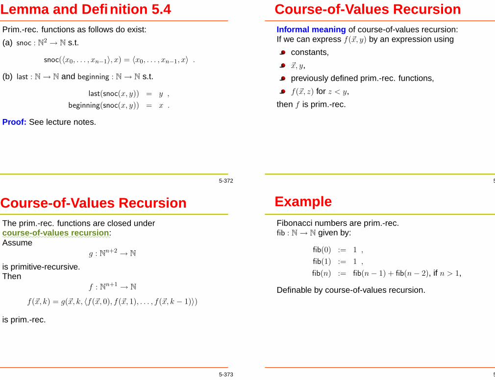
Lemma and Definition 5.4Prim.-rec. functions as follows do exist:

(a) snoc : N2 → N s.t.

snoc(〈x0, . . . , xn−1〉, x) = 〈x0, . . . , xn−1, x〉 .

(b) last : N → N and beginning : N → N s.t.

last(snoc(x, y)) = y ,

beginning(snoc(x, y)) = x .


5-372

Course-of-Values RecursionThe prim.-rec. functions are closed under::::::::::::::::::::::

course-of-values:::::::::::::

recursion:Assume

g : Nn+2 → N

is primitive-recursive.Then

f : Nn+1 → N

f(~x, k) = g(~x, k, 〈f(~x, 0), f(~x, 1), . . . , f(~x, k − 1)〉)

is prim.-rec.

5-373

Course-of-Values RecursionInformal meaning of course-of-values recursion:If we can express f(~x, y) by an expression using

constants,

~x, y,

previously defined prim.-rec. functions,

f(~x, z) for z < y,

then f is prim.-rec.

5-374

ExampleFibonacci numbers are prim.-rec.fib : N → N given by:

fib(0) := 1 ,

fib(1) := 1 ,

fib(n) := fib(n − 1) + fib(n − 2), if n > 1,

Definable by course-of-values recursion.

5-375

ProofProof that prim.-rec. functions are closed undercourse-of-values recursion:Let

f(~x, y) := g(~x, k, 〈f(~x, 0), f(~x, 1), . . . , f(~x, k − 1)〉)

Show f is prim. rec.Define h : Nn+1 → N,

h(~x, y) := 〈f(~x, 0), f(~x, 1), . . . , f(~x, y − 1)〉 .

(Especially, h(~x, 0) = 〈〉.)

5-376

Proof

f(~x, y) := g(~x, k, 〈f(~x, 0), f(~x, 1), . . . , f(~x, k − 1)〉)h(~x, y) := 〈f(~x, 0), f(~x, 1), . . . , f(~x, y − 1)〉 .

h(~x, 0) = 〈〉 ,

h(~x, y + 1) = 〈f(~x, 0), f(~x, 1), . . . , f(~x, y − 1), f(~x, y)〉= snoc(〈f(~x, 0), f(~x, 1), . . . , f(~x, y − 1)〉︸︷︷︸

=h(~x,y)

, f(~x, y))

= snoc(h(~x, y), g(~x, y, 〈f(~x, 0), f(~x, 1), . . . , f(~x, y − 1)〉︸︷︷︸=h(~x,y)

))

= snoc(h(~x, y), g(~x, y, h(~x, y))) .

Therefore h is primitive-recursive.

5-377

Proof

f(~x, y) := g(~x, k, 〈f(~x, 0), f(~x, 1), . . . , f(~x, k − 1)〉)h(~x, y) := 〈f(~x, 0), f(~x, 1), . . . , f(~x, y − 1)〉 .

h is prim.-rec.

Now we have that

f(~x, y) = (〈f(~x, 0), . . . , f(~x, y)〉)y+1

= (h(~x, y + 1))y+1


5-378

Lemma and Definition 5.6There exists prim.-rec. functions as follows:

(a) append : N2 → N s.t.

append(〈n0, . . . , nk−1〉, 〈m0, . . . ,ml−1〉) = 〈n0, . . . , nk−1,m0, . . . ,ml−1〉 .

We write n ∗ m for append(n,m).

(b) subst : N3 → N, s.t. if i < n then

subst(〈x0, . . . , xn−1〉, i, y) = 〈x0, . . . , xi−2, y, xi, xi+1, . . . , xn−1〉 ,

and if i ≥ n, then

subst(〈x0, . . . , xn−1〉, i, y) = 〈x0, . . . , xn−1〉 .

We write x[i/y] for subst(x, i, y).

5-379

Lemma and Definition 5.6(c) substring : N3 → N s.t., if i < n,

substring(〈x0, . . . , xn−1〉, i, j) = 〈xi, xi+1, . . . , xmin(j−1,n−1)〉 ,

and if i ≥ n,

substring(〈x0, . . . , xn−1〉, i, j) = 〈〉 .

5-380

Lemma and Definition 5.6(d) half : N → N,

s.t. half(n) = k if n = 2k or n = 2k + 1.

(e) The function bin : N → N, s.t.bin(n) = 〈b0, . . . , bk〉,for bi in normal form (no leading zeros, unless n = 0),s.t. n = (b0, . . . , bk)2

(f) A function bin−1 : N → N, s.t.bin−1(〈b0, . . . , bk〉) = n, if (b0, . . . , bk)2 = n.

5-381

Ackermann FunctionThe

:::::::::::::::

Ackermann:::::::::::

function Ack : N2 → N is defined as

Ack(n,m) := Ackn(m) .

Therefore we have the equations

Ack(0, y) = y + 1 ,

Ack(x + 1, 0) = Ack(x, 1) ,

Ack(x + 1, y + 1) = Ack(x,Ack(x + 1, y)) .

5-382

Lemma 5.8For each n, m, the following holds:

(a) Ack(m,n) > n.

(b) Ackm is strictly monotone,i.e. Ack(m,n + 1) > Ack(m,n).

(c) Ack(m + 1, n) > Ack(m,n).

(d) Ack(m,Ack(m,n)) < Ack(m + 2, n).

(e) Ack(m, 2n) < Ack(m + 2, n).

(f) Ack(m, 2k · n) < Ack(m + 2k, n).


5-383

Lemma 5.9Every primitive-recursive function f : Nn → N can bemajorised by one branch of the Ackermann function:

There exists N s.t.

f(x0, . . . , xn−1) < AckN (x0 + · · · + xn−1)

for all x0, . . . , xn−1 ∈ N.

Especially, if f : N → N is prim.-rec., then there exists an Ns.t.

∀x ∈ N.f(x) < AckN (x)


5-384

Lemma 5.10The Ackermann function is not primitive-recursive.

Proof:Assume Ack were primitive-recursive.Then

f : N → N, f(n) := Ack(n, n)

is prim.-rec.Then there exists an N ∈ N, s.t. f(n) < Ack(N,n) for all n.Especially

Ack(N,N) = f(N) < Ack(N,N) ,

a contradiction.

5-385

RemarkDirect argument for the existence of non-primitive-recursivecomputable functions:Assume all computable functions are prim.-rec..Define h : N2 → N,

h(e, n) =

f(n), if e encodes a string in ASCIIwhich is a term denoting a unaryprimitive-recursive function f ,

0, otherwise.

h is computable, therefore primitive-recursive.

h can be considered as an interpreter for the language of

primitive recursive functions.

5-386

RemarkIf e code for f , then h(e, n) = f(n).h is prim.-rec.For every primitive-recursive function f there exists a codee of f , therefore

∀n.h(e, n) = f(n) ,

f = λn.h(e, n) .

Definef : N → N, f(n) := h(n, n) + 1 .

f is defined in such a way, that it cannot be of the formλn.h(e, n): If it were, we would get

h(e, e) + 1 = f(e) = (λn.h(e, n))(e) = h(e, e) .

5-387

RemarkIf e code for f , then h(e, n) = f(n).h is prim.-rec.f(n) := h(n, n) + 1.f 6= λn.h(e, n).h is primitive-recursive, therefore as well f .Therefore h = λn.h(e, n), which cannot be the case.Therefore we obtain a contradiction.

5-388

Extension of the aboveThe above proof can be used in other contexts as well.It shows as well that there is no programming language,which computes all computable functions and such that allfunctions definable in this language are total.If we had such a language, then we could define codes e forprograms in this language,and therefore we could define a computable h : N2 → N, s.t.

h(e, n) =

f(n), if e is a program in this languagefor a unary function f ,

0, otherwise.

Using essentially the same argument as before we get acontradiction.

5-389

Extension of the aboveThe above proof shows as well that by adding theAckermann function as basic function to the definition ofprimitive-recursive functions, or any other functions, we stillwon’t obtain all computable functions

– the above argument can be used for for such sets of func-

tions in just the same way as for the set of primitive-recursive

functions.

5-390

Limitations of Prim.-Rec. Functs.We can define prim.-rec. functions which

compute the result of running n steps of a URM or TM,

check whether a URM or TM has stopped,

obtain, depending on n arguments the initialconfiguration for computing P (n) for a URM P or M (n)

for a TM M ,

extract from a configuration of P and M , in which thismachine has stopped, the result optained by M (n), P (n).

Formally done for TMs in Subsection 5.6.

5-391

Limitations of Prim.-Rec. Functs.However, TMs and URMs don’t allow to compute an n,s.t. after n steps the URM or TM has stopped.

Extension of prim.-rec. functions by adding to theprinciples of forming functions closure under µ.

Resulting set called the set of::::::::

partial:::::::::::::

recursive::::::::::::::

functions.

Using the µ-operator, we will be able to find the first ns.t. a TM or URM stops.

Therefore one can show that all TM- andURM-computable functions are partial recursive.

5-392

Limitations of Prim.-Rec. Functs.µ(f) might be partial, even if f is total.⇒ Resulting set is set of partial functions, thereforename partial recursive functions.

The::::::::::::

recursive functions will be the partial recursivefunctions, which are total.

5-393

Partial Rec. FunctionsInductive definition of the set of::::::::

partial:::::::::::::

recursive:::::::::::::

functions ftogether with their

::::::

arity,i.e. together with the k s.t. f : Nk ∼→ N.We write “f : Nk ∼→ N is partial recursive” for “f is partialrecursive with arity k”, and N for N1.

The following:::::::

basic:::::::::::::

functions are partial recursive:

zero : N∼→ N,

succ : N∼→ N,

projki : Nk ∼→ N (0 ≤ i ≤ k).

5-394

Partial Rec. FunctionsIf

g : Nk ∼→ N is partial recursive,

for i = 0, . . . , k − 1 we have hi : Nn ∼→ N is partialrecursive,

then g ◦ (h0, . . . , hk−1) : Nn ∼→ N is partial recursive aswell.As before we write g ◦ h instead of g ◦ (h),g0 ◦ g1 ◦ g2 ◦ · · · ◦ gn for g0 ◦ (g1 ◦ (g2 ◦ · · · ◦ gn)).

5-395

Partial Rec. FunctionsIf

g : Nn ∼→ N,

h : Nn+2 ∼→ N are partial recursive,

then primrec(g, h) : Nn+1 ∼→ N is partial recursive as well.

Ifk ∈ N,

h : N2 ∼→ N is partial recursive,

then primrec(k, h) : N∼→ N is partial recursive as well.

5-396

Partial Rec. FunctionsIf g : Nk+2 ∼→ N is partial recursive,then µ(g) : Nk+1 ∼→ N is partial recursive as well.(Remember that f := µ(g) has defining equation

f(~x) '

min{k ∈ N |g(~x, k) ' 0

∧ ∀l < k.g(~x, l) ↓}, if such a k exists,undefined, otherwise.)

5-397

Recursive Functions(a) A

::::::::::::

recursive:::::::::::

function is a partial recursive function,which is total.

(b) A::::::::::::

recursive:::::::::::

relation is a relation R ⊆ Nn s.t. χR isrecursive.

Example:Ack is recursive, but not primitive-recursive.

5-398

Closure of Part. Rec. Func.Every prim.-rec. function (relation) is recursive.

The recursive functions and relations have the sameclosure properties as those discussed for the prim.-rec.functions and relations.

5-399

Closure of Part. Rec. Func.Let for a predicate U ⊆ Nn+1

µz.U(~n, z) :=

{min{z | U(~n, z)}, if such a z exists,undefined, otherwise.

Then we have that, if U is recursive, so is the function

f(~n) :' µz.U(~n, z) .

Proof:f(~n) ' µz.(χNn\U (~n, z) ' 0) .

5-400

Lemma 5.13All partial recursive functions are URM computable.

Proof: By Lemma 3.3.

5-401

TM-Computable Implies Part.-Rec.We will define for TMs M a code code(M) ∈ N andshow:

For n ∈ N there exist partial rec. func.

fn : Nn+1 ∼→ N

s.t. for every TM M we have

∀~m ∈ Nn.fn(code(M), ~m) ' M (n)(~m) .

fn will be called::::::::::::

universal:::::::::

partial:::::::::::::

recursive::::::::::::

functions.fn can be seen as an interpreter for TM.

5-402

TM-Computable Implies Part.-Rec.fn : Nn+1 → N,∀~m ∈ Nn.fn(code(M), ~m) ' M (n)(~m).

We will later write {e}n(~m) for fn(e, ~m).

The brackets in {e}n are called “Kleene-brackets”, sinceKleene introduced this notation.

5-403

Encoding of TMSeveral Steps needed for this.

Use of::::::::::::::::::::

Gödel-brackets in order to denote the code ofan object:

E.g. dxe for the code of x.

Assume encoding dxe for symbols x of the alphabet of aTM s.t.

d0e = 0,d1e = 1,dxye = 2.

5-404

Encoding of TMWe assume that codes dqe for states q s.t. dq0e = 0 forthe initial state q0 of the TM.

We encode the directions in the instructions bydLe = 0,dRe = 1.

We assume the alphabet consists of {0, 1, xy} andsymbols occurring in the instructions.

⇒ no need to explicitly mention the alphabet in thecode for a TM.

We assume the states consists of {q0} and the statesoccurring in the instructions.

⇒ no need to explicitly mention the set of states inthe code for a TM.

5-405

Encoding of TMNo need to mention q0, xy.⇒ TM can be identified with its instructions.

An instruction I = (q, a, q′, a′, D) will be encoded as

code(I) = π5(dqe, dae, dq′e, da′e, dDe) .

A set of instructions {I0, . . . , Ik−1} will be encoded as

〈code(I0), . . . , code(Ik−1)〉 .

This is as well code(M) of the corresponding TM.

5-406

Encoding of a ConfigurationConfiguration of a TM given by:

The code dqe of its state q.

A segment (i.e. a consecutive sequence of cells) of thetape, which includes

the cell at head position,all cells which are not blank.

A segment a0, . . . , an−1 is encoded as

code(a0, . . . , an−1) := 〈da0e, . . . , dan−1e〉 .

The position of the head on this tape.Given as a number i s.t. 0 ≤ i < n, if the segmentrepresented is a0, . . . , an−1.

5-407

Encoding of a ConfigurationA configuration of a TM, given by

a state q,

a segment a0, . . . , an−1,

head position i,

will be encoded as

π3(dqe, code(a0, . . . , an−1), i) .

5-408

Simulation of TM – symbol, stateWe define primitive-recursive functionssymbol, state : N → N,which extract

the symbol at the head,the state of the TM

from the current configuration:

symbol(a) = (π31(a))π3

2(a)

state(a) = π30(a)

Note that a = π3(dqe, 〈da0e, . . . , dan−1e〉, i).

5-409

Simulation of TM – lookupWe define a prim.-rec. function

lookup : N3 → N ,

s.t. ife is the code for a TM,q state,a a symbol,

then lookup(e, q, a) is a number

π3(dq′e, da′e, dDe)

for the first instruction of the TM e of the form(q, a, q′, a′, D), if it exists.

5-410

Simulation of TM – lookupIf no such instruction exists, the result will be0(= π3(0, 0, 0)).lookup is defined as follows:

First find using bounded search the index of the firstinstruction starting with dqe, da′e.Then extract the corresponding values from thisinstruction.

Details are in the notes.

5-411

Simulation of TM – hasinstructionThere exists a primitive-recursive relationhasinstruction ⊆ N3, s.t.

hasinstruction(e, dqe, dae) holds, iff the TMcorresponding to e has a instruction (q, a, q′, a′, D) forsome q′, a′, D.hasinstruction is defined as a byproduct of defininglookup.

5-412

Simulation of TM – nextThere exists prim rec. function

next : N2 → N

s.t.if e encodes a TMand c is a code for a configuration,

thennext(e, c) is a code for the configuration after one stepof the TM is executed,or equal to c, if the TM has halted.

5-413

Simulation of TM – nextInformal description of next:

Assume the configuration is

c = π3(q, 〈a0, . . . , an−1〉, i) .

Check using hasinstruction, whether the TM hasstopped.If it has stopped, return c.Otherwise, use lookup to obtain the codes for

the next state q′,next symbol a′,direction D.

Replace in 〈a0, . . . , an−1〉, the ith element by a′.Let the result be x.

5-414

Simulation of TM – nextNext state is q′, next Symbol is a′, direction is D.x = result of subsituting the symbol in original segment.

Might be that head will leave segment.Then extend segment.

Case D = dLe and i = 0:Extend the segment to the left by one blank.Result of next is

π3(q′, 〈dxye〉 ∗ x, 0) .

Case D 6= dLe, i ≥ n − 1.Result of next is

π3(q′, x ∗ 〈dxye〉, n) .

5-415

Simulation of TM – nextNext state is q′, next Symbol is a′, direction is D.x = result of subsituting the symbol in original segment.

Otherwise leti′ := i − 1, if D = dLe,i′ := i + 1, if D 6= dLe.

Result of next isπ3(q′, x, i′) .

5-416

Simulation of TM – terminateThere exists a prim.-rec. predicate terminate ⊆ N2, s.t.terminate(e, c) holds, iff the TM e with configuration cstops:

terminate(e, c) :⇔ ¬hasinstruction(e, state(c), symbol(c)) .

5-417

Simulation of TM – iterateThere exists a primitive-recursive functioniterate : N3 → N,s.t. iterate(e, c, n) is the result of iterating TM e with initialconfiguration c for n steps.The definition is as follows

iterate(e, c, 0) = c ,

iterate(e, c, n + 1) = next(e, iterate(e, c, n)) .

5-418

Simulation of TM – initThere exists a primitive-recursive functioninitn : Nn → N,s.t. for any TM M containing alphabet {0, 1, xy}initn(~m) is the initial configuration for computing M (n)(~m)for any TM M , the alphabet of which contains {0, 1, xy}:

initn(m0, . . . ,mn−1)

= π3(dq0e, bin(m0) ∗ 〈dxye〉 ∗ bin(m1) ∗ 〈dxye〉 ∗ · · ·∗ 〈dxye〉 ∗ bin(mn−1), 0) .

5-419

Simulation of TM – extractThere exists a primitive-recursive functionextract : N → N, s.t.

if c is a configuration in which the TM stops,extract(c) is the natural number corresponding to theresult returned by the TM.

Assume c = π3(q, x, i).

extract(c) obtained by applying bin−1 to the largestsubsequence of x starting at i consisting of 0 and 1 only.

5-420

Simulation of TM – TThere exist primitive-recursive predicates Tn ⊆ Nn+2

s.t.,if e encodes a TM M , thenTn(e,m0, . . . ,mn−1, k) holds, iff M ,

started with the initial configuration corresponding toa computation of M (n)(m0, . . . ,mn−1),stops after π0(k) steps,and has final configuration π1(k).

Tn(e, ~m, k) :⇔terminate(e, iterate(e, initn(~m), π0(k)))

∧ iterate(e, initn(~m), π0(k)) = π1(k) .

5-421

Simulation of TM – UThere exists a prim.-rec. function U : N → N s.t. if

M is a TM with code(M) = e,Tn(e, ~m, k) holds,

then U(k) is the result of M (n)(~m).

U(k) = extract(π1(k)) .

Therefore, if e encodes a TM M , then

M (n)(~n) ' U(µz.Tn(e, ~m, z)) .

5-422

Kleene’s NF TheoremKleene’s Normal Form Theorem 5.14:

(a) There exists partial recursive functions fn : Nn+1 ∼→ N

s.t.if e is the code of TM M then

fn(e, ~n) ' Mn(~n) .

(b) There exista primitive-recursive function U : N → N,primitive recursive predicate Tn ⊆ Nn+2,

s.t. for the function fn introduced in (a) we have

fn(e, ~n) ' U(µz.Tn(e, ~m, z)) .

5-423

Definition 5.15Let U, Tn as in Kleene’s Normal Form Theorem 5.14.Then define for e ∈ N the partial recursive function

{e}n : Nn ∼→ N

by{e}n(~m) ' U(µy.Tn(e, ~m, y)) .

{e}n(~m) is pronounced

:::::::::::::::::::::::

Kleene-Brackets-e::

in:::

n::::::::::::::

arguments:::::::::

applied::::

to:::

~m.

5-424

Corollary 5.16

(a) For every TM-computable function f : Nn ∼→ N thereexists e ∈ N s.t.

f = {e}n .

(b) Especially, all TM-computable functions are partialrecursive.

5-425

Theorem 5.17The following sets coincide:

the set of URM-computable functions,

the set of Turing-computable functions,

the set of partial recursive functions.

Proof:

URM-computable implies TM-computable by Theorem4.3.

TM-computable implies partial recursive by Corollary5.16.

Partial recursive implies URM computable by Lemma5.13.

5-426

RemarkBy Kleene’s Normal Form Theorem everyTM-computable function g : Nn ∼→ N is of the form {e}n.Since the TM-computable functions are the partial rec.functions, we obtain:

The partial recursive functions g : Nn ∼→ N are ex-actly the functions {e}n.

This means:{e}n is partial recursive for every e ∈ N.

For every partial recursive function g : Nn ∼→ N thereexists an e s.t. g = {e}n.

5-427

RemarkTherefore

fn : Nn+1 ∼→ N , fn(e, ~x) ' {e}n(~x)

forms a universal n-ary partial recursive function:It encodes all n-ary partial recursive function.

So we can assign to each partial recursive function g anumber, namely an e s.t. g = {e}n.

Each number e denotes one partial recursivefunction {e}n.However, several numbers denote the same partialrecursive function:There are e, e′ s.t. e 6= e′ but {e}n = {e′}n.

5-428

Proof of Last FactProof, that different e compute the same function:

There are several algorithms for computing the samefunction.

Therefore there are several Turing machines whichcompute the same function.

These Turing machines have different codes e.

5-429

Lemma 5.18The set F of partial recursive functions

(and therefore as well of Turing-computable and ofURM-computable functions),

i.e.

F := {f : Nk ∼→ N | k ∈ N ∧ f partial recursive}

is countable.

5-430

Proof of Lemma 5.18Every partial recursive function is of the form {e}n for somee, n ∈ N.

Therefore

f : N2 → F , f(e, n) := {e}n

is surjective,

therefore as well

g : N → F , g(e) := f(π0(e), π1(e)) .

Therefore F is countable.

5-431

The Church-Turing ThesisWe have introduced three models of computations:

The URM-computable functions.

The Turing-computable functions.

The partial recursive functions.

Further we have shown that all three models compute thesame partial functions.

6-432

The Church-Turing ThesisLots of other models of computation have been studied:

The while programs.

Symbol manipulation systems by Post and by Markov.

Equational calculi by Kleene and by Gödel.

The λ-definable functions.

Any of the programming languages Pascal, C, C++,Java, Prolog, Haskell, ML (and many more).

Lots of other models of computation.

6-433

The Church-Turing ThesisOne can show that the partial functions computable inthese models of computation are again exactly thepartial recursive functions.

So all these attempts to define a complete model ofcomputation result in the same set of partial recursivefunctions.

Therefore we arrive at the Church Turing Thesis

6-434

The Church-Turing Thesis

Church-Turing Thesis: The (in an intu-itive sense) computable partial functions areexactly the partial recursive functions (orequivalently the URM-computable or Turing-computable functions).

6-435

Philosophical ThesisThis thesis is not a mathematical theorem.

It is a philosophical thesis.

Therefore the Church-Turing thesis cannot be proven.

We can only provide philosophical evidence for it.

This evidence comes from the followingconsiderations and empirical facts:

6-436

Empirical FactsAll complete models of computation suggested byresearchers define the same set of partial functions.

Many of these models were carefully designed in orderto capture intuitive notions of computability:

The Turing machine model captures the intuitivenotion of computation on a piece of paper in ageneral sense.The URM machine model captures the generalnotion of computability by a computer.Symbolic manipulation systems capture the generalnotion of computability bymanipulation of symbolic strings.

6-437

Empirical FactsNo intuitively computable partial function, which is notpartial recursive, has been found, despite lots ofresearchers trying it.

A strong intuition has been developed that in principalprograms in any programming language can besimulated by Turing machines and URMs.

Because of this, only few researchers doubt the correctnessof the Church-Turing thesis.

6-438

Halting ProblemBecause of the equivalence of these models, the haltingproblem for any of the above mentioned models ofcomputation is undecidable.

Especially it is undecidable, whether a program in oneof the programming languages mentioned terminates:

Assume we had a decision procedure for decidingwhether or not say a Pascal program terminates forgiven input.Then we could, using a translation of URMs intoPascal programs, decide the halting problem forURMs, which is impossible.

6-439

Sec. 7 The Recursion TheoremMain result in this section:Kleene’s Recursion Theorem.

Recursive functions are closed under a very generalform of recursion.

For proof we will use the S-m-n-theorem.Used in many proofs in computability theory.

7-440

The S-m-n TheoremAssume f : Nm+n ∼→ N partial recursive.

Fix the first m arguments (say l0, . . . , lm−1).

Then we obtain a partial recursive function

g : Nn ∼→ N , g(~x) = f(l0, . . . , lm−1, ~x) .

The S-m-n theorem expresses that we can compute aKleene index of g

i.e. an e′ s.t. g = {e′}n

from a Kleene index of f and l0, . . . , lm−1

primitive-recursively.

7-441

The S-m-n Theoremf : Nm+n ∼→ N partial rec.g(~x) = f(l0, . . . , lm−1, ~x).

So there exists a primitive-recursive function Smn s.t.,

if f = {e}m+n,then g = {Sm

n (e, l0, . . . , lm−1)}n.

7-442

Theorem 7.1 (S-m-n Theorem)Assume m,n ∈ N.

There exists a primitive-recursive function

Smn : Nm+1 → N

s.t. for all ~l, ~x ∈ N

{Smn (e,~l)}n(~x) ' {e}m+n(~l, ~x) .

7-443

Proof of S-m-n TheoremLet M be a TM encoded as e.

A Turing machine M ′ corresponding to Smn (e,~l) should

be s.t.M ′n(~x) ' Mn+m(~l, ~x) .

7-444

Proof of S-m-n TheoremM is TM for e.Want to define M ′ s.t. M ′n(~x) ' Mn+m(~l, ~x)M ′ can be defined as follows:

1. The initial configuration is:~x written on the tape,head pointing to the left most bit:

· · · xy xy bin(x0) xy · · · xy bin(xn−1) xy xy · · ·↑

7-445

Proof of S-m-n TheoremM is TM for e.Want to define M ′ s.t. M ′n(~x) ' Mn+m(~l, ~x)Initial configuration:· · · xy xy bin(x0) xy · · · xy bin(xn−1) xy xy · · ·

↑

2. M ′ writes first binary representation of l0, . . . , lm−1 infront of this.terminates this step with the head pointing to themost significant bit of bin(l0).

So configuration after this step is:

bin(l0) xy · · · xy bin(lm−1) xy bin(x0) xy · · · xy bin(xn−1)

↑

7-446

Proof of S-m-n TheoremM is TM for e.Want to define M ′ s.t. M ′n(~x) ' Mn+m(~l, ~x).Configuration after first step:bin(l0) xy · · · xy bin(lm−1) xy bin(x0) xy · · · xy bin(xn−1)

↑

Then M ′ runs M , starting in this configuration.It terminates, if M terminates.The result is

' Mm+n(~l, ~x) ,

and we get therefore

M ′n(~x) ' Mm+n(~l, ~x)

as desired.7-447

Proof of S-m-n TheoremM is TM for e.M ′ is a TM s.t. M ′n(~x) ' Mn+m(~l, ~x)

From a code for M one can now obtain a code for M ′ ina primitive-recursive way.

Smn is the corresponding function.

More details in the lecture notes.

7-448

NotationWe will usually omit the superscript n in{e}n(m0, . . . ,mn−1)

i.e. write {e}(m0, . . . ,mn−1) instead of{e}n(m0, . . . ,mn−1).

Further {e} not applied to arguments and withoutsuperscript means usually {e}1.

7-449

Kleene’s Recursion TheoremAssume f : Nn+1 ∼→ N partial recursive.

Then there exists an e ∈ N s.t.

{e}n(x0, . . . , xn−1) ' f(e, x0, . . . , xn−1) .

7-450

ExamplesKleene’s Rec. Theorem: ∃e.∀~x.{e}n(~x) ' f(e, ~x).

There exists an e s.t.

{e}(x) ' e + 1 .

For showing this take in the Recursion Theoremf(e, n) := e + 1.Then

{e}(x) ' f(e, x) ' e + 1 .

7-451

ExamplesKleene’s Rec. Theorem: ∃e.∀~x.{e}n(~x) ' f(e, ~x).

Remark:

Such applications usually not very useful.

Usually, when using the Rec. Theorem, onedoesn’t use the index e directly,but only the application of {e} to some arguments.

7-452

Examples2. The function computing the Fibonacci-numbers fib is

recursive.(This is a weaker result than what we obtainedabove –above we showed that it is even prim.-rec.)

7-453

Fibonacci NumbersRemember the defining equations for fib:

fib(0) = fib(1) = 1 ,

fib(n + 2) = fib(n) + fib(n + 1) .

From these equations we obtain

fib(n) =

{1, if n = 0 or n = 1,fib(n−· 2) + fib(n−· 1), otherwise.

We show that there exists a recursive function g : N → N,s.t.

g(n) '{

1, if n = 0 or n = 1,g(n−· 2) + g(n−· 1), otherwise.

7-454

Fibonacci NumbersShow: Exists g rec. s.t.

g(n) '{


Shown as follows: Define a recursive f : N2 → N s.t.

f(e, n) '{

1, if n = 0 or n = 1,{e}(n−· 2) + {e}(n−· 1), otherwise.

Now let e be s.t.{e}(n) ' f(e, n) .

Then e fulfills the equations

{e}(n) '{


7-455

Fibonacci Numbers

{e}(n) '{


Let g = {e}.Then we get

g(n) '{


These are the defining equations for fib.One can show by induction on n that g(n) = fib(n) for alln ∈ N.Therefore fib is recursive.

7-456

General Applic. of Rec. TheoremSimilarly, one can introduce arbitrary partial recursivefunctions g, where

g(~n) refers to arbitrary other values g(~m).This corresponds to the recursive definition of functionsin programming.E.g. in Java one defines

public static int fib(int n){if (n == 0 || n == 1){return 1;}

else{return fib(n-1) + fib(n-2);

}};

7-457

Example 3As in general programming, recursively defined functionsneed not be total:

There exists a partial recursive function g : N∼→ N s.t.

g(x) ' g(x) + 1 .

We get g(x) ↑.

The definition of g corresponds to the following Javadefinition:public static int g(int n){return g(n) + 1;

};When executing g(x), Java loops.

7-458

Example 4

There exists a partial recursive function g : N∼→ N s.t.

g(x) ' g(x + 1) + 1 .

Note that that’s a “black hole recursion”, which is notsolvable by a total function.

It is solved by g(x) ↑.

Note that a recursion equation for a function f can notalways be solved by setting f(x) ↑.

E.g. the recursion equation for fib can’t be solved bysetting fib(n) ↑.

7-459

Ackermann FunctionThe Ackermann function is recursive:Remember the defining equations:

Ack(0, y) = y + 1 ,

Ack(x + 1, 0) = Ack(x, 1) ,

Ack(x + 1, y + 1) = Ack(x,Ack(x + 1, y)) .

From this we obtain

Ack(x, y) =

y + 1, if x = 0,Ack(x−· 1, 1), if x > 0 and y = 0,Ack(x−· 1,Ack(x, y−· 1)), otherwise.

7-460

Ackermann Function

Ack(x, y) =

y + 1, if x = 0,Ack(x−· 1, 1), if x > 0 and y = 0,Ack(x−· 1,Ack(x, y−· 1)), otherwise.

Define g partial recursive s.t.

g(x, y) '

y + 1, if x = 0,g(x−· 1, 1), if x > 0 ∧ y = 0,g(x−· 1, g(x, y−· 1)), if x > 0 ∧ y > 0.

g fulfills the defining equations of Ack.

Proof that g(x, y) ' Ack(x, y) follows by main inductionon x, side-induction on y.

Details: See lecture notes.7-461

Proof of the Rec. TheoremAssume

f : Nn+1 ∼→ N .

We have to find an e s.t.

∀~x ∈ N.{e}n(~x) ' f(e, ~x) .

Idea:Define e = S1

n(e1, e2) for some (yet unknown) e1, e2.We get:

{e}n(~x) ' {S1n(e1, e2)}n(~x) ' {e1}n+1(e2, ~x) .

So we need to find e1, e2 s.t.

∀~x. {e1}n+1(e2, ~x)︸︷︷︸'{e}n(~x)

' f(S1n(e1, e2), ~x)︸︷︷︸'f(e,~x)

.

7-462

Proof of Rec. TheoremNeed to solve:∀~x.{e1}n+1(e2, ~x) ' f(S1

n(e1, e2), ~x).Let e1 s.t.

{e1}n+1(y, ~x) ' f(S1n(y, y), ~x) .

So we need to solve

f(S1n(e1, e2), ~x)︸︷︷︸

'{e1}n+1(e2,~x)

' f(S1n(e2, e2), ~x) .

Can be fulfilled by setting e2 := e1.So, an index solving the problem is

e = S1n(e1, e2) = S1

n(e1, e1) ,

and we are done.

7-463

Short Version of ProofLet e1 be s.t.

{e1}n+1(y, ~x) ' f(S1n(y, y), ~x) .

Let e := S1n(e1, e1).

Then we have

{e}n(~x)e = S1

n(e1, e1)' {S1

n(e1, e1)}n(~x)

S-m-n theorem' {e1}n+1(e1, ~x)

Def of e1' f(S1n(e1, e1), ~x)

e = S1

n(e1, e1)' f(e, ~x) .

7-464

Sec. 8: Rec. Enumerable PredicatesWe study P ⊆ Nn, which are

not decidable,but “half decidable”.

Official name issemi-decidable,or recursively enumerable.

8-465

Rec. SetsRemember:

A predicate A is recursive, iff χA is recursive.

So we have a “full” decision procedure:

P (x0, . . . , xn−1) ⇔ χA(x0, . . . , xn−1) = 1, i.e. answer yes ,

¬P (x0, . . . , xn−1) ⇔ χA(x0, . . . , xn−1) = 0, i.e. answer no .

8-466

Semi-Decidable SetsP ⊆ Nn will be semi-decidable,if there exists a partial recursive recursive function f s.t.

P (x0, . . . , xn−1) ⇔ f(x0, . . . , xn−1) ↓ .

If P (x0, . . . , xn−1) holds,we will eventually know it:the algorithm for computing f will finally terminate,and then we know that P (x0, . . . , xn−1) holds.

If P (x0, . . . , xn−1) doesn’t hold,then the algorithm computing f will loop for ever,and we never get an answer.

8-467

Semi-Decidable SetsSo we have:

P (x0, . . . , xn−1) ⇔ f(x0, . . . , xn−1) ↓ i.e. answer yes ,

¬P (x0, . . . , xn−1) ⇔ f(x0, . . . , xn−1) ↑ i.e. no answerreturned by f .

8-468

ApplicationsOne might think that r.e. sets don’t occur in computing.

But they occur in many applications.

Typical example:

A(x) ⇔ there exists a proof in a certainformal system of a property ϕ(x) .

E.g. ϕ(x) expresses the correctness of a circuitmultiplying two numbers.

8-469

Applications

A(x) ⇔ there exists a proof in a certainformal system of a property ϕ(x).

Assuming “soundness and completeness” (see othermodules), we have:

If we find a proof for ϕ(x), then ϕ(x) holds.If we don’t find a proof, then ϕ(x) doesn’t hold.

8-470

Applications


In many applications the function f s.t.

A(x) ⇔ f(x) ↓

terminates in most practical cases very fast.However, in principal it might take arbitrarily long.

If one then runs f(x), and it takes longer than a certainamount of time, one assumes A(x) is probably false.

Then one uses other means in order to determinethe reason why A(x) is false.

8-471

Applications


If A(x) holds, one expects the algorithm for f(x) toterminate after a certain amount of time.

If this algorithms actually terminates within theexpected amount of time, one knows that ϕ(x) holds.

8-472

Def. 8.1Assume f : Nn ∼→ N.

(a) The::::::::::

domain:::

of::

f , in short dom(f)::::::::

is defined as follows:

dom(f) := {(x0, . . . , xn−1) ∈ Nn | f(x0, . . . , xn−1) ↓} .

(b) The:::::::

range::::

of::

f , in short ran(f)::::::

is defined as follows:

ran(f) := {y ∈ N | ∃x0, . . . , xn−1.(f(x0, . . . , xn−1) ' y)} .

(c) The::::::::

graph:::

of::

f is the set Gf:::

defined as

Gf := {(~x, y) ∈ Nn+1 | f(~x) ' y} .

8-473

Remark on Gf

The notion “graph” used here has nothing to do with thenotion of “graph” in graph theory.

The graph of a function is essentially the graph we drawwhen visualising f .

8-474

Remark on Gf

Example:

f : N∼→ N , f(x) =

{x2 , if x even,undefined, if x is odd.

We can draw f as follows:

3

4

2

1

1 2 3 4 5 6 70

08-475

Remark on Gf

In this example we have

Gf = {(0, 0), (2, 1), (4, 2), (6, 3), . . .}

These are exactly the coordinates of the crosses in thepicture:

3

4

2

1

1 2 3 4 5 6 70

0

(0,0) (2,1)(4,2)

(6,3)

8-476

Def. Recursively EnumerableA predicate A ⊆ Nn is

::::::::::::::

recursively::::::::::::::::

enumerable,in short

::::

r.e.,if there exists a partial recursive function f : Nn ∼→ N s.t.

A = dom(f) .

Sometimes recursive predicates are as well called

::::::::::::::::::::

semi-decidable or

::::::::::::::::::::::

semi-computable or

::::::::::

partially::::::::::::::::

computable.

8-477

Lemma 8.3(a) Every recursive predicate is r.e.

(b) The halting problem, i.e.

Haltn(e, ~x) :⇔ {e}n(~x) ↓ ,

is r.e., but not recursive.

Proof: See notes.

8-478

Theorem 8.4There exist r.e. predicates

Wn ⊆ Nn+1

s.t., with

Wne := {(x0, . . . , xn−1) ∈ Nn | Wn(e, x0, . . . , xn−1) ,

we have the following:

Each of the predicates Wne ⊆ Nn is r.e.

For each r.e. predicate P ⊆ Nn there exists an e ∈ N s.t.P = Wn

e , i.e.

∀~x ∈ N.P (~x) ⇔ Wne (~x) .

8-479

Theorem 8.4Therefore, the r.e. sets P ⊆ Nn are exactly the sets Wn

e fore ∈ N.

8-480

Remark on Theorem 8.4Wn

e ist therefore auniversal recursively enumerable sets, whichencodes all other recursively enumerable sets.

The theorem means that that we can assign to everyrecursively enumerable predicate A a natural number,namely the e s.t. A = Wn

e .Each code denotes one predicate.However, several numbers denote the samepredicate:

there are e, e′ s.t. e 6= e′ but Wne = Wn

e′.(Since there are e 6= e′ s.t. {e}n = {e′}n).

8-481

Proof Idea for Theorem 8.4

Wne := dom({e}n) .

If A is r.e., then A = dom(f) for some partial rec. f .Let f = {e}n.Then A = Wn

e .Details: See lecture notes.

8-482

Theorem 8.5Let A ⊆ Nn. The following is equivalent:

(i) A is r.e.

(ii)A = {~x | ∃y.R(~x, y)}

for some primitive-recursive predicate R.

(iii)A = {~x | ∃y.R(~x, y)}

for some recursive predicate R.

(iv)A = {~x | ∃y.R(~x, y)}

for some recursively enumerable predicate R.

8-483

Theorem 8.5(i) A is r.e.

(v) A = ∅ or

A = {(f0(x), . . . , fn−1(x)) | x ∈ N}for some primitive-recursive functions

fi : N → N .

(vi) A = ∅ or

A = {(f0(x), . . . , fn−1(x)) | x ∈ N}

for some recursive functions

fi : N → N .

8-484

RemarkWe can summarise Theorem 8.5 as follows:There are 3 equivalent ways of defining that A ⊆ Nn isr.e.:

A = dom(f) for some partial recursive f ;A = ∅ or A is the image of primitiverecursive/recursive functions f0, . . . , fn−1;A = {~x | ∃y.R(~x, y)} for someprimitive-recursive/recursive/r.e. R.

8-485

Remark, Case n = 1

For A ⊆ N the following is equivalent:A is r.e.A = ∅ orA = ran(f) for some primitive-recursive f : N → N .

A = ∅ or A = ran(f) for some recursive f : N → N .

Therefore A ⊆ N is r.e. ifA = ∅or there exists a (prim.-)rec. function f , whichenumerates all its elements.

This explains the name “recursively enumerablepredicate”.

8-486

ProofProof of Theorem 8.5: See notes.Proof Ideas:

(i) → (ii):Assume A is r.e., A = dom(f), for f partial recursive.

A(~x) ⇔ f(~x) ↓⇔ ∃y.the TM for computing f(~x) terminates

after y steps

⇔ ∃y.R(~x, y)

where

R(~x, y) ⇔ the TM for comp. f(~x) termin. after y steps .

R is primitive-recursive. 8-487

Proof Ideas(ii) → (v), special case n = 1:Assume

A = {x ∈ N | ∃y.R(x, y)} where R is prim.-rec.A 6= ∅,y ∈ A fixed.

Define f : N → N recursive,

f(x) =

{π0(x), if R(π0(x), π1(x)),y otherwise.

Then A = ran(f).

8-488

Proof Ideas(v), (vi) → (i), special case n = 1:Assume

A = ran(f) ,

where f is (prim.-)recursive.Then

A = dom(g) ,

whereg(x) ' (µy.f(y) = x) .

g is partial recursive.

8-489

Theorem 8.6A ⊆ Nk is recursive iff both A and Nk \ A are r.e.

Proof idea:“⇒” is easy.For “⇐”: Assume

A(~x) ⇔ ∃y.R(~x, y)

(Nk \ A)(~x) ⇔ ∃y.S(~x, y)

In order to decide A, search simultaneously for a y s.t.R(~x, y) and for a y s.t. S(~x, y) holds.If we find a y s.t. R(~x, y) holds, then A(~x) holds.

If we find a y s.t. S(~x, y) holds, then ¬A(~x) holds

8-490

Theorem 8.7Let f : Nn ∼→ N.Then

f is partial recursive ⇔ Gf is r.e. .

Proof idea for “⇐”:Assume R primitive recursive s.t.

Gf (~x, y) ⇔ ∃z.R(~x, y, z) .

In order to compute f(~x), search for a y s.t.R(~x, π0(y), π1(y)) holds.f(~x) will be the first projection of this y.

8-491

Lemma 8.8The recursively enumerable sets are closed under:

Union:If A,B ⊆ Nn are r.e. so is A ∪ B.

Intersection:If A,B ⊆ Nn are r.e. so is A ∩ B.

Substitution by recursive functions:If A ⊆ Nn is r.e., fi : Nk → N are recursive fori = 0, . . . , n, so is

C := {(y0, . . . , yk−1) ∈ Nk |A(f0(y0, . . . , yk−1), . . . , fn−1(y0, . . . , yk−1)) .

8-492

Lemma 8.8(Unbounded) existential quantification:If D ⊆ Nn+1 is r.e., so is

E := {(x0, . . . , xn−1) ∈ Nn | ∃y.D(x0, . . . , xn−1, y)} .

Bounded universal quantification:If D ⊆ Nn+1 is r.e., so is

F := {(x0, . . . , xn−1, z) ∈ Nn+1 | ∀y < z.D(x0, . . . , xn−1, z)} .

8-493

Lemma 8.9The r.e. predicates are not closed under complement:

There exists an r.e. predicate A ⊆ Nn s.t. Nn \ A is not r.e.

Proof idea:Haltn is r.e. but not recursive.Therefore Nn \ Haltn is not r.e.

8-494

philosophy. - cs.swan.ac.ukcsetzer/lectures/computability/03/cpslidesdraft... · the truth of...

Documents