Syllabus Computability Theory

Sebastiaan A. Terwijn

Institute for Discrete Mathematics and GeometryTechnical University of ViennaWiedner Hauptstrasse 8–10/E104A-1040 Vienna, Austriaterwijn@logic.at

Copyright c© 2004 by Sebastiaan A. TerwijnCover picture and above close-up:Sunflower drawing by Alan Turing,c© copyright by University of Southampton andKing’s College Cambridge 2002, 2003.

iii

Emil Post (1897–1954) Alonzo Church (1903–1995)

Kurt Godel (1906–1978)

Stephen Cole Kleene(1909–1994)

Alan Turing (1912–1954)

Contents

1 Introduction 1

1.1 Preliminaries . . . . . . . . . . . . . . . . . . . . . . . . . . . . . . . . 2

2 Basic concepts 3

2.1 Algorithms . . . . . . . . . . . . . . . . . . . . . . . . . . . . . . . . . 3

2.2 Recursion . . . . . . . . . . . . . . . . . . . . . . . . . . . . . . . . . . 4

2.2.1 The primitive recursive functions . . . . . . . . . . . . . . . . . 4

2.2.2 The recursive functions . . . . . . . . . . . . . . . . . . . . . . 5

2.3 Turing machines . . . . . . . . . . . . . . . . . . . . . . . . . . . . . . 6

2.4 Arithmetization . . . . . . . . . . . . . . . . . . . . . . . . . . . . . . . 9

2.4.1 Coding functions . . . . . . . . . . . . . . . . . . . . . . . . . . 10

2.4.2 The normal form theorem . . . . . . . . . . . . . . . . . . . . . 10

2.4.3 The basic equivalence and Church’s thesis . . . . . . . . . . . . 13

2.4.4 Canonical coding of finite sets . . . . . . . . . . . . . . . . . . . 15

2.5 Exercises . . . . . . . . . . . . . . . . . . . . . . . . . . . . . . . . . . 15

3 Computable and computably enumerable sets 18

3.1 Diagonalization . . . . . . . . . . . . . . . . . . . . . . . . . . . . . . . 18

3.2 Computably enumerable sets . . . . . . . . . . . . . . . . . . . . . . . 18

3.3 Undecidable sets . . . . . . . . . . . . . . . . . . . . . . . . . . . . . . 21

3.4 Uniformity . . . . . . . . . . . . . . . . . . . . . . . . . . . . . . . . . 22

3.5 Many-one reducibility . . . . . . . . . . . . . . . . . . . . . . . . . . . 24

3.6 Simple sets . . . . . . . . . . . . . . . . . . . . . . . . . . . . . . . . . 25

3.7 The recursion theorem . . . . . . . . . . . . . . . . . . . . . . . . . . . 26

3.8 Exercises . . . . . . . . . . . . . . . . . . . . . . . . . . . . . . . . . . 28

4 The arithmetical hierarchy 30

4.1 The arithmetical hierarchy . . . . . . . . . . . . . . . . . . . . . . . . . 30

4.2 Computing levels in the arithmetical hierarchy . . . . . . . . . . . . . 33

4.3 Exercises . . . . . . . . . . . . . . . . . . . . . . . . . . . . . . . . . . 35

5 Relativized computation and Turing degrees 36

5.1 Turing reducibility . . . . . . . . . . . . . . . . . . . . . . . . . . . . . 36

5.2 The jump operator . . . . . . . . . . . . . . . . . . . . . . . . . . . . . 37

5.3 Limit computable sets . . . . . . . . . . . . . . . . . . . . . . . . . . . 38

5.4 Incomparable degrees . . . . . . . . . . . . . . . . . . . . . . . . . . . 39

5.5 Inverting the jump . . . . . . . . . . . . . . . . . . . . . . . . . . . . . 40

5.6 Exercises . . . . . . . . . . . . . . . . . . . . . . . . . . . . . . . . . . 41

v

6 The priority method 436.1 Diagonalization, again . . . . . . . . . . . . . . . . . . . . . . . . . . . 436.2 A pair of Turing incomparable c.e. sets . . . . . . . . . . . . . . . . . . 446.3 Exercises . . . . . . . . . . . . . . . . . . . . . . . . . . . . . . . . . . 45

7 Applications 467.1 Undecidability in logic . . . . . . . . . . . . . . . . . . . . . . . . . . . 467.2 Constructivism . . . . . . . . . . . . . . . . . . . . . . . . . . . . . . . 497.3 Randomness and Kolmogorov complexity . . . . . . . . . . . . . . . . 507.4 Exercises . . . . . . . . . . . . . . . . . . . . . . . . . . . . . . . . . . 51

Further reading 53

Bibliography 54

vi

Chapter 1

Introduction

In this syllabus we discuss the basic concepts of computability theory, also called re-cursion theory. There are various views as to what computability theory is. Odifreddi[17, 18] defines it very broadly as the study of functions of natural numbers. Anotherview is to see the subject as the study of definability (Slaman), thus stressing theconnections with set theory. But the most commonly held view is to see it as thestudy of computability of functions of natural numbers. The restriction to functionsof natural numbers is, certainly at the start of our studies, a very mild one since, aswe will see, the natural numbers possess an enormous coding power so that many ob-jects can be presented by them in one way or another. It is also possible to undertakethe study of computability on more general domains, leading to the subject of highercomputability theory (Sacks [24]), but we will not treat this in this syllabus.

In the choice of material for this syllabus we have made no effort to be original,but instead we have tried to present a small core of common and important notionsand results of the field that have become standard over the course of time. The partwe present by no means includes all the standard material, and we refer the reader tothe “further reading” section for much broader perspectives. The advantage of ournarrow view is that we can safely say that everything we do here is important.

As a prerequisite for reading this syllabus only a basic familiarity with mathemat-ical language and formalisms is required. In particular our prospective student willneed some familiarity with first-order logic. There will also be an occasional referenceto cardinalities and set theory, but a student not familiar with this can simply skipthese points.

The outline of the syllabus is as follows. In Chapter 2 we introduce the basicconcepts of computability theory, such as the formal notion of algorithm, recursivefunction, and Turing machine. We show that the various formalizations of the in-formal notion of algorithm all give rise to the same notion of computable function.This beautiful fact is one of the cornerstones of computability theory. In Chapter 3we discuss the basic properties of the computable and computably enumerable (c.e.)sets, and venture some first steps into the uncomputable. In Chapters 4 and 5 weintroduce various measures to study unsolvability: In Chapter 4 we study the arith-metical hierarchy and m-degrees, and in Chapter 5 we study relative computabilityand Turing degrees. In Chapter 6 we introduce the priority method, and use it toanswer an important question about the Turing degrees of c.e. sets. Finally, in Chap-ter 7 we give some applications of computability theory. In particular we give a proofof Godels incompleteness theorem.

1

2 Chapter 1. Introduction

1.1 Preliminaries

Our notation is standard and follows the textbooks [17, 27]. ω is the set of naturalnumbers {0, 1, 2, 3 . . . }. By set we usually mean a subset of ω. The Cantor space 2ω

is the set of all subsets of ω. We often identify sets with their characteristic functions:For A ⊆ ω we often identify A with the function χA : ω → {0, 1} defined by

χA(n) =

{1 if n ∈ A

0 otherwise.

The complement ω−A is denoted by A. By a (total) function we will always mean afunction from ωn to ω, for some n. We use the letters f , g, h to denote total functions.The composition of two functions f and g is denoted by f ◦ g. A partial function isa function from ω to ω that may not be defined on some arguments. By ϕ(n) ↓ wedenote that ϕ is defined on n, and by ϕ(n) ↑ that it is undefined. The domain ofa partial function ϕ is the set dom(ϕ) =

{x : ϕ(x) ↓

}, and the range of ϕ is the

set rng(ϕ) ={y : (∃x)[ϕ(x) = y]

}. We use the letters ϕ and ψ, to denote partial

functions. For such partial functions, ϕ(x) = ψ(x) will mean that either both valuesare undefined, or both are defined and equal. For notational convenience we willoften abbreviate a finite number of arguments x1, . . . , xn by ~x. We will make use ofthe λ-notation for functions: λx1 . . . xn.f(x1, . . . , xn) denotes the function mapping~x to f(~x). The set of all finite binary strings is denoted by 2<ω. We use σ and τfor finite strings. The length of σ is denoted by |σ|, and the concatenation of σ andτ is denoted by σ τ . That τ is an subsequence (also called initial segment) of σ isdenoted by τ v σ. For a set A, A�n denotes the finite string A(0)A(1) . . .A(n−1)consisting of the first n bits of A.

At the end of every chapter are the exercises for that chapter. Some exercises aremarked with a ? to indicate that they are more challenging.

Chapter 2

Basic concepts

2.1 Algorithms

An algorithm is a finite procedure or a finite set of rules to solve a problem in astep by step fashion. The name algorithm derives from the name of the 9th centurymathematician al-Khwarizmi and his book ”Al-Khwarizmi Concerning the Hindu Artof Reckoning”, which was translated in Latin as “Algoritmi de numero Indorum.” Forexample, the recipe for baking a cake is an algorithm, where the “problem” is thetask of making a cake. However, the word algorithm is mostly used in more formalcontexts. The procedure for doing long divisions is an example of an algorithm thateveryone learns in school. Also, every computer program in principle constitutes analgorithm, since it consists of a finite set of rules determining what to do at everystep.

For many centuries there did not seem a reason to formally define the notion ofalgorithm. It was a notion where the adagium “you recognize it when you see one”applied. This became different at the turn of the 20th century when problems suchas the following were addressed:

• (The “Entscheidungsproblem”, ) Given a logical formula (from the first-orderpredicate logic), decide whether it is a tautology (i.e. valid under all interpre-tations) or not. This problem can be traced back to Leibniz [13].

• (Hilberts Tenth Problem) Given a Diophantine equation, that is a polynomialin several variables with integer coefficients, decide whether it has a solutionin the integers. This problem comes from a famous list of problems posed byHilbert at the end of the 19th century [8].

A positive solution to these problems would consist of an algorithm that solves them.But what if such an algorithm does not exist? If one wants to settle the aboveproblems in the negative, i.e. show that there exists no algorithm that solves them,one first has to say precisely what an algorithm is. That is, we need a formal definitionof the informal notion of algorithm. This is the topic of this first chapter.

There are many ways to formalize the notion of algorithm. Quite remarkably, allof these lead to the same formal notion! This gives us a firm basis for a mathematicaltheory of computation: computability theory. Below, we give two of the most famousformalizations: recursive functions and Turing computable functions. We then pro-ceed by proving that these classes of functions coincide. As we have said, there aremany other formalizations. We refer the reader to Odifreddi [17] for further examples.

3

4 Chapter 2. Basic concepts

Returning to the above two problems: With the help of computability theoryit was indeed proven that both problems are unsolvable, i.e. that there exist noalgorithms for their solution. For the Entscheidungsproblem this was proved inde-pendently by Church [2] and Turing [29] (see Theorem 7.1.6), and for Hilberts TenthProblem by Matijasevich [15], building on work of Davis, Putnam, and Robinson.

2.2 Recursion

The approach to computability using the notion of recursion that we consider in thissection is the reason that computability theory is also commonly known under thename recursion theory. This approach was historically the first and is most famousfor its application in Godels celebrated incompleteness results [7], cf. Section 7.1. Infact, although the statements of these results do not mention computability, Godelinvented some of the basic notions of computability theory in order to prove hisresults.

2.2.1 The primitive recursive functions

Recursion is a method to define new function values from previously defined functionvalues. Consider for example the famous Fibonacci sequence

1, 1, 2, 3, 5, 8, 13, 21, 34 . . .

which was discovered by Fibonacci in 1202. Every term in the sequence is obtainedby taking the sum of the two previous terms: F (n+2) = F (n+1)+F (n). To get thesequence started we define F (0) = 1 and F (1) = 1. This sequence occurs in manyforms in nature, for example in the phyllotaxis of seeds in sunflowers (see Turingsdrawing on the cover). Counting in clockwise direction we can count 21 spirals, andcounting counterclockwise yields 34 spirals. In this and in many other cases (e.g.in pineapples or daisies) the numbers of these two kinds of spirals are always twoconsecutive Fibonacci numbers. (Cf. also Exercises 2.5.1 and 2.5.2.) In general, afunction f is defined by recursion from given functions g and h if an initial value f(0)is defined (using g) and for every n, f(n+1) is defined (using h) in terms of previousvalues. The idea is that if we can compute g and h, then we can also compute f .Thus recursion is a way to define more computable functions from given ones.

Definition 2.2.1 (Primitive recursion, Dedekind [3]) A function f is defined fromfunctions g and h by primitive recursion if

f(~x, 0) = g(~x)

f(~x, n+ 1) = h(f(~x, n), ~x, n).

In this definition, f(n + 1) is defined in terms of the previous value f(n). A moregeneral form of recursion, where f(n + 1) is defined in terms of f(0), . . . , f(n) istreated in Exercise 2.5.8.

Definition 2.2.2 (Primitive recursive functions, Godel [7]) The class of primitiverecursive functions is the smallest class of functions

2.2. Recursion 5

1. containing the initial functions

O = λx.0 (constant zero function)

S = λx.x+ 1 (successor function)

πin = λx1, . . . , xn.xi 1 ≤ i ≤ n, (projection functions)

2. closed under composition, i.e. the schema that defines

f(~x) = h(g1(~x), . . . , gn(~x))

from the given functions h and gi.

3. closed under primitive recursion.

For example, Grassmann gave in 1861 the following recursive definitions for the usualinteger addition + and multiplication · :

x+ 0 = x

x+ S(y) = S(x+ y),

x · 0 = 0

x · S(y) = (x · y) + x.

Note that the first recursion reduces the definition of + to the initial function S, andthat the second reduces multiplication to addition. For a precise proof that + and ·are primitive recursive see Exercise 2.5.3.

2.2.2 The recursive functions

Note that all primitive recursive functions are total functions. We will now give aninformal argument showing that it is essential for our theory to also consider partialfunctions.

In any formalization of the notion of algorithm, an algorithm will be definedsyntactically by a finite set of symbols. In this sense every algorithmically computablefunction will be a finite object. Now since the theory will require us to recognize aneffectively manipulate these objects, it is natural that there should also be an effectiveway to list all computable functions by a listing of their algorithms: There should bea computable function f such that f(n) is a code for the n-th algorithm, computingthe n-th computable function fn. Now suppose that we would only consider totalfunctions. Then the function F = λn.fn(n)+1 would also be a computable function,the m-th in the list, say. But then

F (m) = fm(m) 6= fm(m) + 1 = F (m),

a contradiction. Note that the contradiction arises since we assumed that the valuefm(m) is always defined. This assumption is dropped if we also include partial func-tions in our theory.

The above discussion suggests that the class of primitive recursive functions is notbig enough to capture the intuitive notion of computable function. Hence we add anew operator to our basic tool kit: the µ-operator. For a predicate R,

(µn)[R(~x, n)

]

6 Chapter 2. Basic concepts

denotes the least number n such that R(~x, n) holds. If such n does not exist then(µn)[R(~x, n)] is undefined. Thus the µ operator allows us to search for certain values.Since such a search can be unbounded, the µ-operator can take us out of the domainof total functions.

Definition 2.2.3 (Recursive functions, Kleene [10]) The class of partial recursivefunctions is the smallest class of functions

1. containing the initial functions

2. closed under composition and primitive recursion

3. closed under µ-recursion, i.e. the schema that defines the partial function

ϕ(~x) = (µy)[(∀z ≤ y)[ψ(~x, z)↓] ∧ ψ(~x, y) = 0

]

from a given partial function ψ.

A (general) recursive function is a partial recursive function that happens to be total.

Note that in the schema of µ-recursion the µ-operator searches for a smallest y suchthat ψ(~x, y) = 0, but that it cannot “jump” over undefined values of ψ because ofthe first clause. This corresponds with the intuition that the search for such a y isperformed by discarding values z for which we can see that ψ(~x, z) 6= 0. Also, as wewill later see, it is undecidable whether a computable function converges, so droppingthe clause would give us a class which is too large. (See also Exercise 2.5.13.)

Clearly, since the class of partial recursive functions contains partial functions, itstrictly extends the class of primitive recursive functions. However, there are also totalexamples showing that the addition of the µ-operator allows us to define more totalfunctions than just the primitive recursive ones. Examples will be easy to construct(cf. Exercise 2.5.11) as soon as we have developed the theory a bit more, in particularafter we have treated the method of arithmetization. This method will also allowus to turn the informal discussion from the beginning of this section into a formalexample.

2.3 Turing machines

In this section we consider a completely different formalization of the notion of al-gorithm, namely the one using Turing machines [29]. Instead of inductively buildingfunctions from previous ones, as in the definition of recursive function, this approachinvestigates directly what it means to perform a computation of a function, using anidealized device or machine. We imagine a tape of unbounded length, consisting ofinfinitely many cells, extending in a one-way infinite row from left to right say. Eachcell may contain a 0, a 1, or a blank, i.e. nothing. We imagine further that we ma-nipulate the symbols on the tape in a completely prescribed way, according to a setof rules or a program. The basic operations that we can perform while scanning a cellare to change its content and to move either left or right. The action that we performmay depend on the content of the cell and on the current state of the program. Theactions we thus perform may or may not terminate. In the latter case we say that wehave completed a computation, and may consider the content of the tape to be itsoutcome. To model the intuition that our actions should be of limited complexity werequire that there can be only finitely many states in the program. Instead of our-selves performing the computation we can also imagine a device containing a program

2.3. Turing machines 7

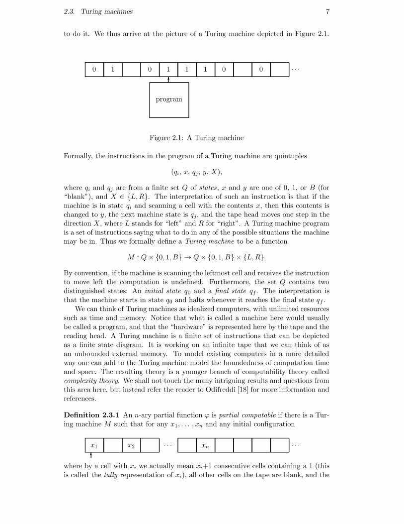
to do it. We thus arrive at the picture of a Turing machine depicted in Figure 2.1.

0 1 0 1 1 1 0 0 · · ·6

program

Figure 2.1: A Turing machine

Formally, the instructions in the program of a Turing machine are quintuples

(qi, x, qj, y, X),

where qi and qj are from a finite set Q of states, x and y are one of 0, 1, or B (for“blank”), and X ∈ {L,R}. The interpretation of such an instruction is that if themachine is in state qi and scanning a cell with the contents x, then this contents ischanged to y, the next machine state is qj, and the tape head moves one step in thedirection X, where L stands for “left” and R for “right”. A Turing machine programis a set of instructions saying what to do in any of the possible situations the machinemay be in. Thus we formally define a Turing machine to be a function

M : Q× {0, 1, B} → Q× {0, 1, B} × {L,R}.

By convention, if the machine is scanning the leftmost cell and receives the instructionto move left the computation is undefined. Furthermore, the set Q contains twodistinguished states: An initial state q0 and a final state qf . The interpretation isthat the machine starts in state q0 and halts whenever it reaches the final state qf .

We can think of Turing machines as idealized computers, with unlimited resourcessuch as time and memory. Notice that what is called a machine here would usuallybe called a program, and that the “hardware” is represented here by the tape and thereading head. A Turing machine is a finite set of instructions that can be depictedas a finite state diagram. It is working on an infinite tape that we can think of asan unbounded external memory. To model existing computers in a more detailedway one can add to the Turing machine model the boundedness of computation timeand space. The resulting theory is a younger branch of computability theory calledcomplexity theory. We shall not touch the many intriguing results and questions fromthis area here, but instead refer the reader to Odifreddi [18] for more information andreferences.

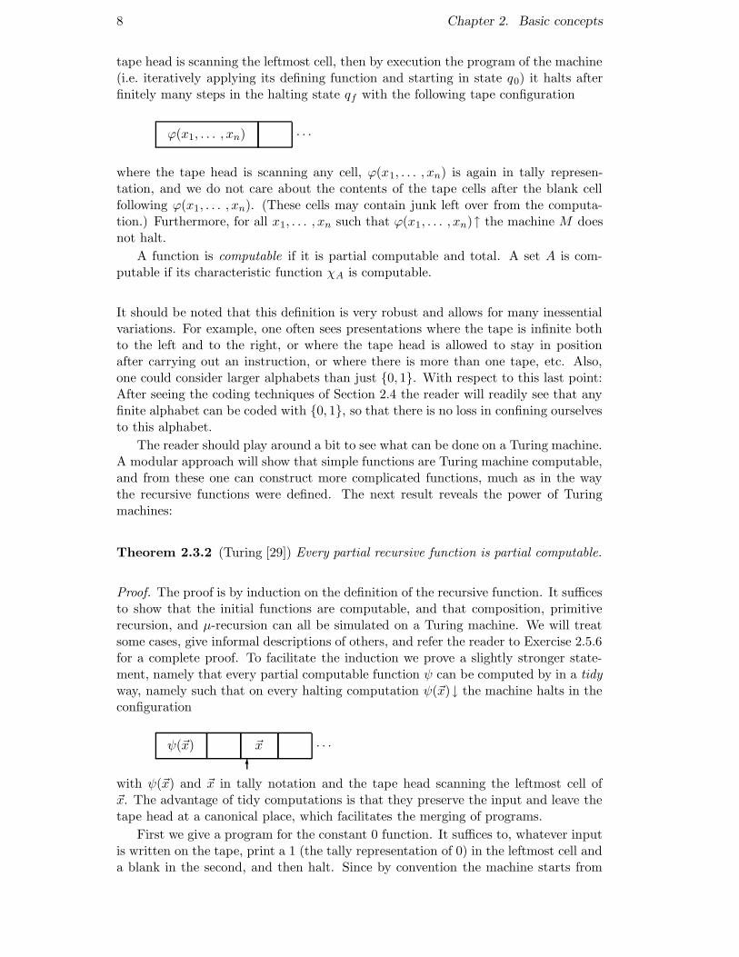
Definition 2.3.1 An n-ary partial function ϕ is partial computable if there is a Tur-ing machine M such that for any x1, . . . , xn and any initial configuration

x1 x2 · · · xn · · ·6

where by a cell with xi we actually mean xi+1 consecutive cells containing a 1 (thisis called the tally representation of xi), all other cells on the tape are blank, and the

8 Chapter 2. Basic concepts

tape head is scanning the leftmost cell, then by execution the program of the machine(i.e. iteratively applying its defining function and starting in state q0) it halts afterfinitely many steps in the halting state qf with the following tape configuration

ϕ(x1, . . . , xn) · · ·

where the tape head is scanning any cell, ϕ(x1, . . . , xn) is again in tally represen-tation, and we do not care about the contents of the tape cells after the blank cellfollowing ϕ(x1, . . . , xn). (These cells may contain junk left over from the computa-tion.) Furthermore, for all x1, . . . , xn such that ϕ(x1, . . . , xn)↑ the machine M doesnot halt.

A function is computable if it is partial computable and total. A set A is com-putable if its characteristic function χA is computable.

It should be noted that this definition is very robust and allows for many inessentialvariations. For example, one often sees presentations where the tape is infinite bothto the left and to the right, or where the tape head is allowed to stay in positionafter carrying out an instruction, or where there is more than one tape, etc. Also,one could consider larger alphabets than just {0, 1}. With respect to this last point:After seeing the coding techniques of Section 2.4 the reader will readily see that anyfinite alphabet can be coded with {0, 1}, so that there is no loss in confining ourselvesto this alphabet.

The reader should play around a bit to see what can be done on a Turing machine.A modular approach will show that simple functions are Turing machine computable,and from these one can construct more complicated functions, much as in the waythe recursive functions were defined. The next result reveals the power of Turingmachines:

Theorem 2.3.2 (Turing [29]) Every partial recursive function is partial computable.

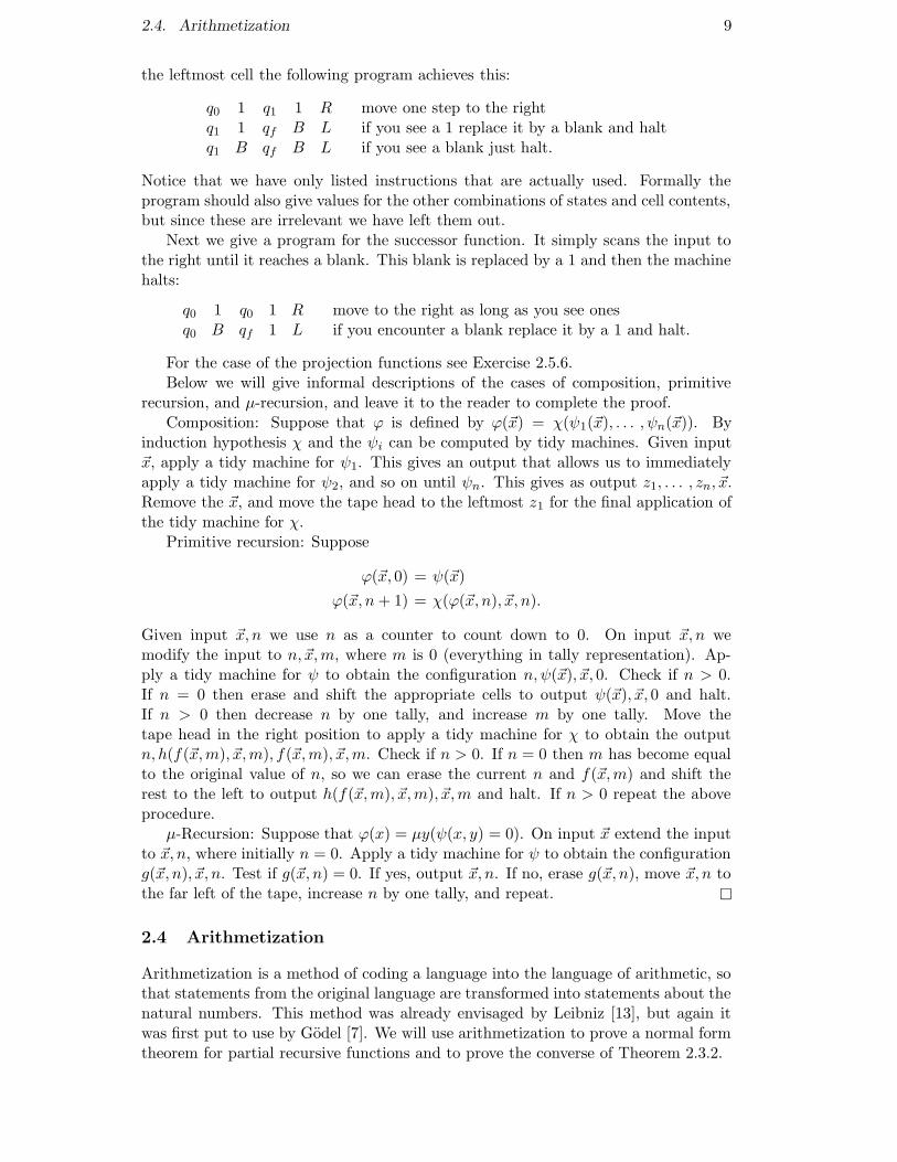
Proof. The proof is by induction on the definition of the recursive function. It sufficesto show that the initial functions are computable, and that composition, primitiverecursion, and µ-recursion can all be simulated on a Turing machine. We will treatsome cases, give informal descriptions of others, and refer the reader to Exercise 2.5.6for a complete proof. To facilitate the induction we prove a slightly stronger state-ment, namely that every partial computable function ψ can be computed by in a tidyway, namely such that on every halting computation ψ(~x)↓ the machine halts in theconfiguration

ψ(~x) ~x · · ·6

with ψ(~x) and ~x in tally notation and the tape head scanning the leftmost cell of~x. The advantage of tidy computations is that they preserve the input and leave thetape head at a canonical place, which facilitates the merging of programs.

First we give a program for the constant 0 function. It suffices to, whatever inputis written on the tape, print a 1 (the tally representation of 0) in the leftmost cell anda blank in the second, and then halt. Since by convention the machine starts from

2.4. Arithmetization 9

the leftmost cell the following program achieves this:

q0 1 q1 1 R move one step to the rightq1 1 qf B L if you see a 1 replace it by a blank and haltq1 B qf B L if you see a blank just halt.

Notice that we have only listed instructions that are actually used. Formally theprogram should also give values for the other combinations of states and cell contents,but since these are irrelevant we have left them out.

Next we give a program for the successor function. It simply scans the input tothe right until it reaches a blank. This blank is replaced by a 1 and then the machinehalts:

q0 1 q0 1 R move to the right as long as you see onesq0 B qf 1 L if you encounter a blank replace it by a 1 and halt.

For the case of the projection functions see Exercise 2.5.6.Below we will give informal descriptions of the cases of composition, primitive

recursion, and µ-recursion, and leave it to the reader to complete the proof.Composition: Suppose that ϕ is defined by ϕ(~x) = χ(ψ1(~x), . . . , ψn(~x)). By

induction hypothesis χ and the ψi can be computed by tidy machines. Given input~x, apply a tidy machine for ψ1. This gives an output that allows us to immediatelyapply a tidy machine for ψ2, and so on until ψn. This gives as output z1, . . . , zn, ~x.Remove the ~x, and move the tape head to the leftmost z1 for the final application ofthe tidy machine for χ.

Primitive recursion: Suppose

ϕ(~x, 0) = ψ(~x)

ϕ(~x, n+ 1) = χ(ϕ(~x, n), ~x, n).

Given input ~x, n we use n as a counter to count down to 0. On input ~x, n wemodify the input to n, ~x,m, where m is 0 (everything in tally representation). Ap-ply a tidy machine for ψ to obtain the configuration n, ψ(~x), ~x, 0. Check if n > 0.If n = 0 then erase and shift the appropriate cells to output ψ(~x), ~x, 0 and halt.If n > 0 then decrease n by one tally, and increase m by one tally. Move thetape head in the right position to apply a tidy machine for χ to obtain the outputn, h(f(~x,m), ~x,m), f(~x,m), ~x,m. Check if n > 0. If n = 0 then m has become equalto the original value of n, so we can erase the current n and f(~x,m) and shift therest to the left to output h(f(~x,m), ~x,m), ~x,m and halt. If n > 0 repeat the aboveprocedure.

µ-Recursion: Suppose that ϕ(x) = µy(ψ(x, y) = 0). On input ~x extend the inputto ~x, n, where initially n = 0. Apply a tidy machine for ψ to obtain the configurationg(~x, n), ~x, n. Test if g(~x, n) = 0. If yes, output ~x, n. If no, erase g(~x, n), move ~x, n tothe far left of the tape, increase n by one tally, and repeat. �

2.4 Arithmetization

Arithmetization is a method of coding a language into the language of arithmetic, sothat statements from the original language are transformed into statements about thenatural numbers. This method was already envisaged by Leibniz [13], but again itwas first put to use by Godel [7]. We will use arithmetization to prove a normal formtheorem for partial recursive functions and to prove the converse of Theorem 2.3.2.

10 Chapter 2. Basic concepts

2.4.1 Coding functions

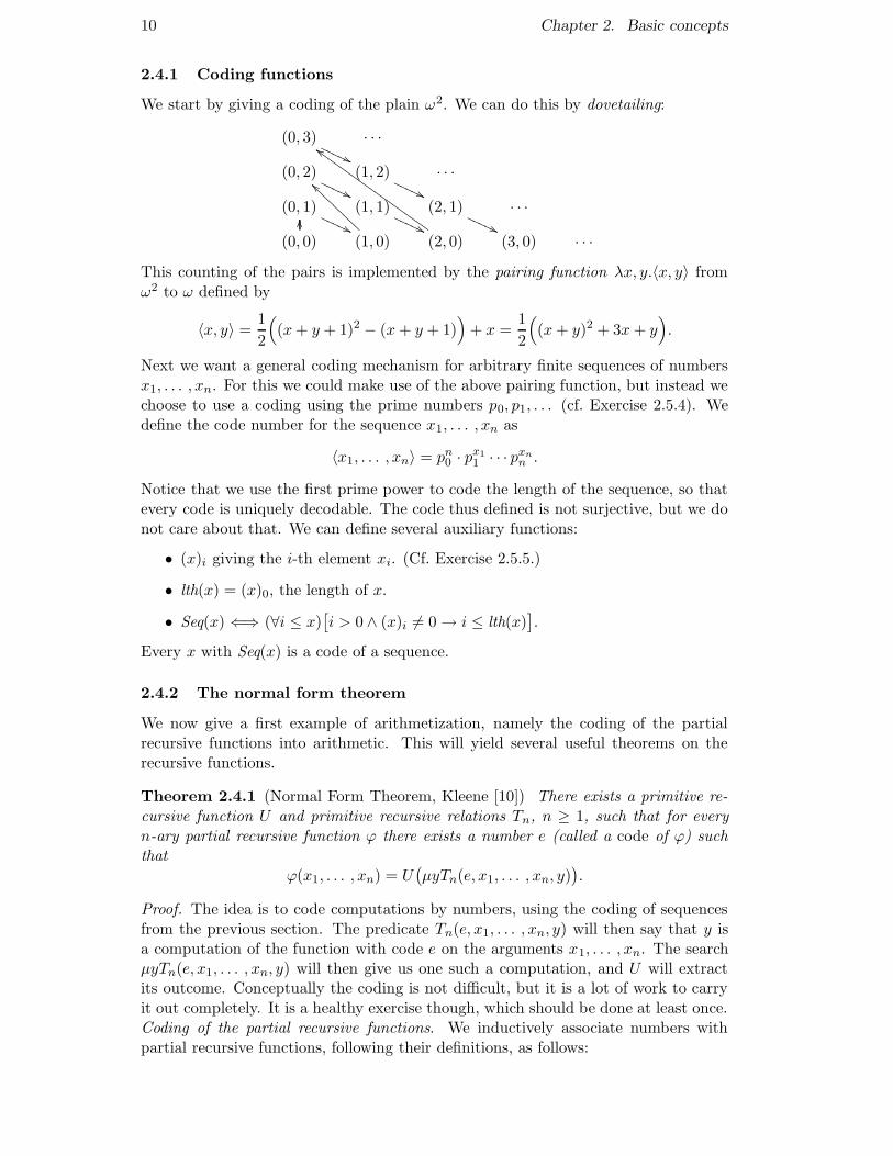
We start by giving a coding of the plain ω2. We can do this by dovetailing:

(0, 3)

''PPPPP. . .

(0, 2)

''PPPPP(1, 2)

''PPPPP. . .

(0, 1)

''PPPPP(1, 1)

''PPPPP(2, 1)

''PPPPP. . .

(0, 0)

OO

(1, 0)

``AAAA

AAAA

A

(2, 0)

ddHHHHHHHHHHHHHHHHHHH

(3, 0) . . .

This counting of the pairs is implemented by the pairing function λx, y.〈x, y〉 fromω2 to ω defined by

〈x, y〉 =1

2

((x+ y + 1)2 − (x+ y + 1)

)+ x =

1

2

((x+ y)2 + 3x+ y

).

Next we want a general coding mechanism for arbitrary finite sequences of numbersx1, . . . , xn. For this we could make use of the above pairing function, but instead wechoose to use a coding using the prime numbers p0, p1, . . . (cf. Exercise 2.5.4). Wedefine the code number for the sequence x1, . . . , xn as

〈x1, . . . , xn〉 = pn0 · px11 · · · pxn

n .

Notice that we use the first prime power to code the length of the sequence, so thatevery code is uniquely decodable. The code thus defined is not surjective, but we donot care about that. We can define several auxiliary functions:

• (x)i giving the i-th element xi. (Cf. Exercise 2.5.5.)

• lth(x) = (x)0, the length of x.

• Seq(x) ⇐⇒ (∀i ≤ x)[i > 0 ∧ (x)i 6= 0 → i ≤ lth(x)

].

Every x with Seq(x) is a code of a sequence.

2.4.2 The normal form theorem

We now give a first example of arithmetization, namely the coding of the partialrecursive functions into arithmetic. This will yield several useful theorems on therecursive functions.

Theorem 2.4.1 (Normal Form Theorem, Kleene [10]) There exists a primitive re-cursive function U and primitive recursive relations Tn, n ≥ 1, such that for everyn-ary partial recursive function ϕ there exists a number e (called a code of ϕ) suchthat

ϕ(x1, . . . , xn) = U(µyTn(e, x1, . . . , xn, y)

).

Proof. The idea is to code computations by numbers, using the coding of sequencesfrom the previous section. The predicate Tn(e, x1, . . . , xn, y) will then say that y isa computation of the function with code e on the arguments x1, . . . , xn. The searchµyTn(e, x1, . . . , xn, y) will then give us one such a computation, and U will extractits outcome. Conceptually the coding is not difficult, but it is a lot of work to carryit out completely. It is a healthy exercise though, which should be done at least once.Coding of the partial recursive functions. We inductively associate numbers withpartial recursive functions, following their definitions, as follows:

2.4. Arithmetization 11

• 〈0〉 corresponds to O

• 〈1〉 to S

• 〈2, n, i〉 to πin

• 〈3, a1, . . . , an, b〉 to ϕ(~x) = χ(ψ1(~x), . . . , ψn(~x)), where a1, . . . , an and b corre-spond to ψ1, . . . , ψn and χ, respectively.

• 〈4, a, b〉 to ϕ(~x, y) defined with primitive recursion from ψ and χ, where a andb correspond to ψ and χ.

• 〈5, a〉 to ϕ(~x) = µy(ψ(~x, y) = 0), where a corresponds to ψ.

Computation trees. We describe computations by trees as follows. Every node in thetree will consist of one computation step.

• At the leaves we write computation computed by the initial functions. So thesesteps are of the form ϕ(x) = 0, ϕ(x) = x+ 1, or ϕ(x1, . . . , xn) = xi.

• Composition: If ϕ(~x) = χ(ψ1(~x), . . . , ψn(~x)) then the node ϕ(~x) = z has then+ 1 predecessors

ψ1(~x) = z1, . . . , ψn(~x) = zm, χ(z1, . . . , zm) = z.

• Primitive recursion: If ϕ(~x, y) is defined with primitive recursion from ψ andχ, then ϕ(~x, 0) = z has predecessor ψ(~x) = z and ϕ(~x, y + 1) has the twopredecessors ϕ(~x, y) = z1 and χ(~x, y, z1) = z.

• µ-recursion: If ϕ(~x) = µy(ψ(~x, y) = 0) then the computation step ϕ(~x) = z hasthe predecessors

ψ(~x, 0) = t0, . . . , ψ(~x, z − 1) = tz−1, ψ(~x, z) = 0

where the ti are all different from 0.

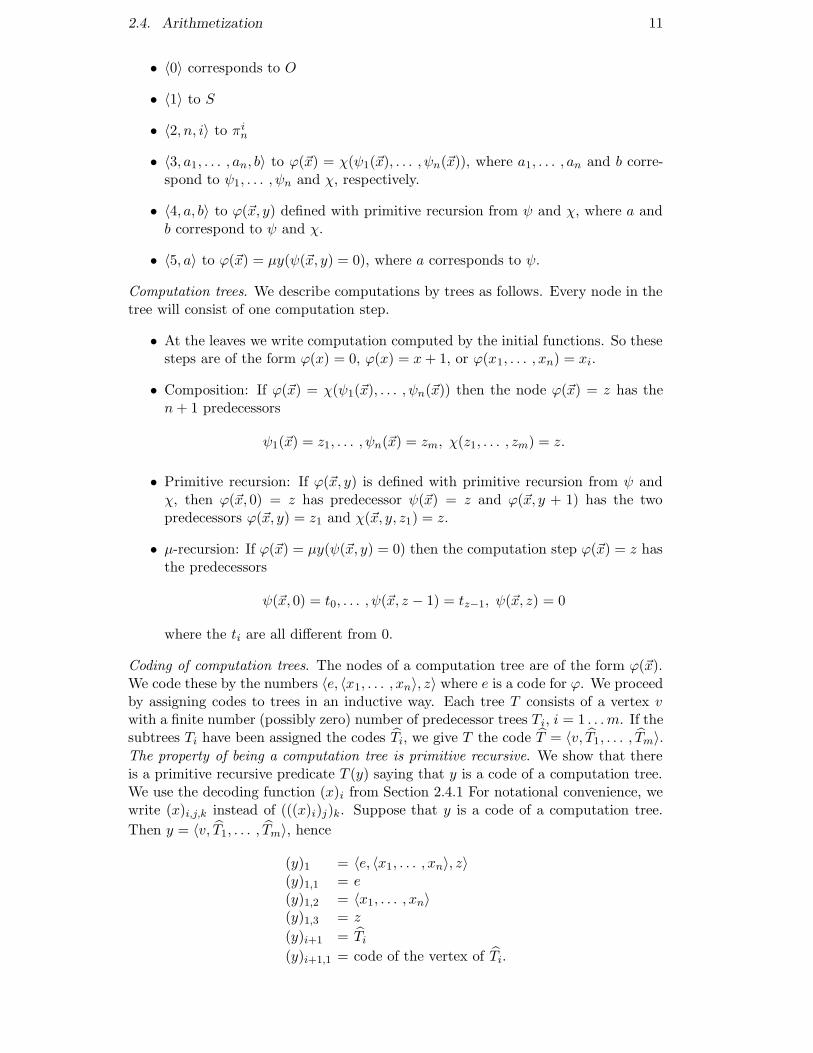
Coding of computation trees. The nodes of a computation tree are of the form ϕ(~x).We code these by the numbers 〈e, 〈x1, . . . , xn〉, z〉 where e is a code for ϕ. We proceedby assigning codes to trees in an inductive way. Each tree T consists of a vertex vwith a finite number (possibly zero) number of predecessor trees Ti, i = 1 . . . m. If thesubtrees Ti have been assigned the codes Ti, we give T the code T = 〈v, T1, . . . , Tm〉.The property of being a computation tree is primitive recursive. We show that thereis a primitive recursive predicate T (y) saying that y is a code of a computation tree.We use the decoding function (x)i from Section 2.4.1 For notational convenience, wewrite (x)i,j,k instead of (((x)i)j)k. Suppose that y is a code of a computation tree.

Then y = 〈v, T1, . . . , Tm〉, hence

(y)1 = 〈e, 〈x1, . . . , xn〉, z〉(y)1,1 = e(y)1,2 = 〈x1, . . . , xn〉(y)1,3 = z

(y)i+1 = Ti(y)i+1,1 = code of the vertex of Ti.

12 Chapter 2. Basic concepts

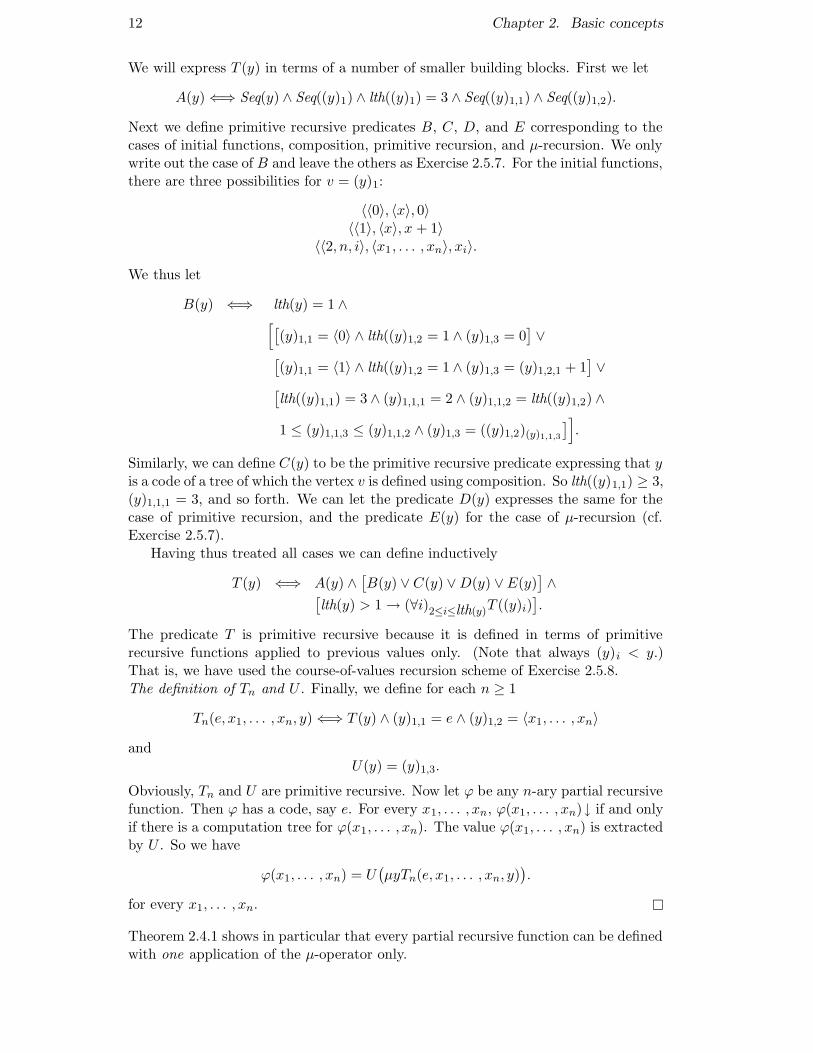
We will express T (y) in terms of a number of smaller building blocks. First we let

A(y) ⇐⇒ Seq(y) ∧ Seq((y)1) ∧ lth((y)1) = 3 ∧ Seq((y)1,1) ∧ Seq((y)1,2).

Next we define primitive recursive predicates B, C, D, and E corresponding to thecases of initial functions, composition, primitive recursion, and µ-recursion. We onlywrite out the case of B and leave the others as Exercise 2.5.7. For the initial functions,there are three possibilities for v = (y)1:

〈〈0〉, 〈x〉, 0〉〈〈1〉, 〈x〉, x + 1〉

〈〈2, n, i〉, 〈x1 , . . . , xn〉, xi〉.

We thus let

B(y) ⇐⇒ lth(y) = 1 ∧[[

(y)1,1 = 〈0〉 ∧ lth((y)1,2 = 1 ∧ (y)1,3 = 0]∨

[(y)1,1 = 〈1〉 ∧ lth((y)1,2 = 1 ∧ (y)1,3 = (y)1,2,1 + 1

]∨

[lth((y)1,1) = 3 ∧ (y)1,1,1 = 2 ∧ (y)1,1,2 = lth((y)1,2) ∧

1 ≤ (y)1,1,3 ≤ (y)1,1,2 ∧ (y)1,3 = ((y)1,2)(y)1,1,3

]].

Similarly, we can define C(y) to be the primitive recursive predicate expressing that yis a code of a tree of which the vertex v is defined using composition. So lth((y)1,1) ≥ 3,(y)1,1,1 = 3, and so forth. We can let the predicate D(y) expresses the same for thecase of primitive recursion, and the predicate E(y) for the case of µ-recursion (cf.Exercise 2.5.7).

Having thus treated all cases we can define inductively

T (y) ⇐⇒ A(y) ∧[B(y) ∨ C(y) ∨D(y) ∨E(y)

]∧[

lth(y) > 1 → (∀i)2≤i≤lth(y)T ((y)i)].

The predicate T is primitive recursive because it is defined in terms of primitiverecursive functions applied to previous values only. (Note that always (y)i < y.)That is, we have used the course-of-values recursion scheme of Exercise 2.5.8.The definition of Tn and U . Finally, we define for each n ≥ 1

Tn(e, x1, . . . , xn, y) ⇐⇒ T (y) ∧ (y)1,1 = e ∧ (y)1,2 = 〈x1, . . . , xn〉

andU(y) = (y)1,3.

Obviously, Tn and U are primitive recursive. Now let ϕ be any n-ary partial recursivefunction. Then ϕ has a code, say e. For every x1, . . . , xn, ϕ(x1, . . . , xn)↓ if and onlyif there is a computation tree for ϕ(x1, . . . , xn). The value ϕ(x1, . . . , xn) is extractedby U . So we have

ϕ(x1, . . . , xn) = U(µyTn(e, x1, . . . , xn, y)

).

for every x1, . . . , xn. �

Theorem 2.4.1 shows in particular that every partial recursive function can be definedwith one application of the µ-operator only.

2.4. Arithmetization 13

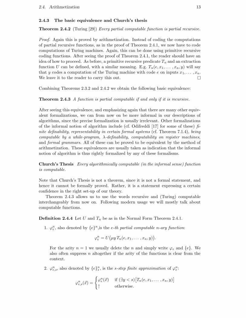
2.4.3 The basic equivalence and Church’s thesis

Theorem 2.4.2 (Turing [29]) Every partial computable function is partial recursive.

Proof. Again this is proved by arithmetization. Instead of coding the computationsof partial recursive functions, as in the proof of Theorem 2.4.1, we now have to codecomputations of Turing machines. Again, this can be done using primitive recursivecoding functions. After seeing the proof of Theorem 2.4.1, the reader should have anidea of how to proceed. As before, a primitive recursive predicate Tn and an extractionfunction U can be defined, with a similar meaning. E.g. Tn(e, x1, . . . , xn, y) will saythat y codes a computation of the Turing machine with code e on inputs x1, . . . , xn.We leave it to the reader to carry this out. �

Combining Theorems 2.3.2 and 2.4.2 we obtain the following basic equivalence:

Theorem 2.4.3 A function is partial computable if and only if it is recursive.

After seeing this equivalence, and emphasizing again that there are many other equiv-alent formalizations, we can from now on be more informal in our descriptions ofalgorithms, since the precise formalization is usually irrelevant. Other formalizationsof the informal notion of algorithm include (cf. Odifreddi [17] for some of these) fi-nite definability, representability in certain formal systems (cf. Theorem 7.1.4), beingcomputable by a while-program, λ-definability, computability on register machines,and formal grammars. All of these can be proved to be equivalent by the method ofarithmetization. These equivalences are usually taken as indication that the informalnotion of algorithm is thus rightly formalized by any of these formalisms.

Church’s Thesis Every algorithmically computable (in the informal sense) functionis computable.

Note that Church’s Thesis is not a theorem, since it is not a formal statement, andhence it cannot be formally proved. Rather, it is a statement expressing a certainconfidence in the right set-up of our theory.

Theorem 2.4.3 allows us to use the words recursive and (Turing) computableinterchangeably from now on. Following modern usage we will mostly talk aboutcomputable functions.

Definition 2.4.4 Let U and Tn be as in the Normal Form Theorem 2.4.1.

1. ϕne , also denoted by {e}n,is the e-th partial computable n-ary function:

ϕne = U(µy Tn(e, x1, . . . , xn, y)

).

For the arity n = 1 we usually delete the n and simply write ϕe and {e}. Wealso often suppress n altogether if the arity of the functions is clear from thecontext.

2. ϕne,s, also denoted by {e}ns , is the s-step finite approximation of ϕne :

ϕne,s(~x) =

{ϕne (~x) if (∃y < s)

[Tn(e, x1, . . . , xn, y)

]

↑ otherwise.

14 Chapter 2. Basic concepts

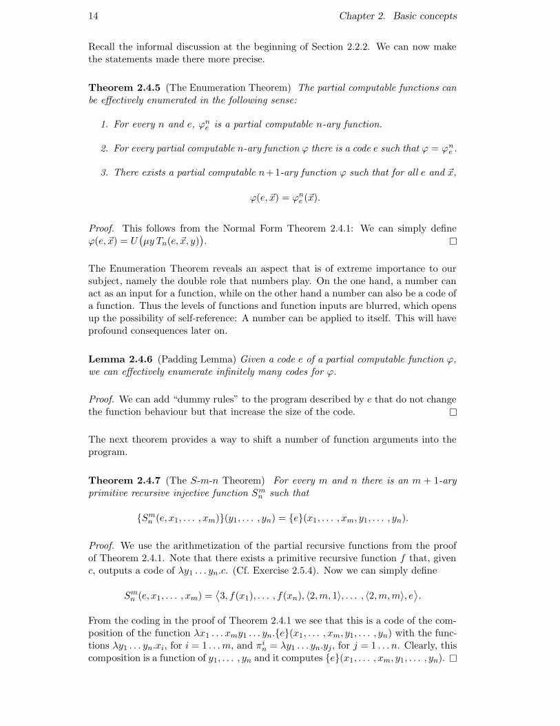
Recall the informal discussion at the beginning of Section 2.2.2. We can now makethe statements made there more precise.

Theorem 2.4.5 (The Enumeration Theorem) The partial computable functions canbe effectively enumerated in the following sense:

1. For every n and e, ϕne is a partial computable n-ary function.

2. For every partial computable n-ary function ϕ there is a code e such that ϕ = ϕne .

3. There exists a partial computable n+1-ary function ϕ such that for all e and ~x,

ϕ(e, ~x) = ϕne (~x).

Proof. This follows from the Normal Form Theorem 2.4.1: We can simply defineϕ(e, ~x) = U

(µy Tn(e, ~x, y)

). �

The Enumeration Theorem reveals an aspect that is of extreme importance to oursubject, namely the double role that numbers play. On the one hand, a number canact as an input for a function, while on the other hand a number can also be a code ofa function. Thus the levels of functions and function inputs are blurred, which opensup the possibility of self-reference: A number can be applied to itself. This will haveprofound consequences later on.

Lemma 2.4.6 (Padding Lemma) Given a code e of a partial computable function ϕ,we can effectively enumerate infinitely many codes for ϕ.

Proof. We can add “dummy rules” to the program described by e that do not changethe function behaviour but that increase the size of the code. �

The next theorem provides a way to shift a number of function arguments into theprogram.

Theorem 2.4.7 (The S-m-n Theorem) For every m and n there is an m + 1-aryprimitive recursive injective function Smn such that

{Smn (e, x1, . . . , xm)}(y1, . . . , yn) = {e}(x1, . . . , xm, y1, . . . , yn).

Proof. We use the arithmetization of the partial recursive functions from the proofof Theorem 2.4.1. Note that there exists a primitive recursive function f that, givenc, outputs a code of λy1 . . . yn.c. (Cf. Exercise 2.5.4). Now we can simply define

Smn (e, x1, . . . , xm) =⟨3, f(x1), . . . , f(xn), 〈2,m, 1〉, . . . , 〈2,m,m〉, e

⟩.

From the coding in the proof of Theorem 2.4.1 we see that this is a code of the com-position of the function λx1 . . . xmy1 . . . yn.{e}(x1, . . . , xm, y1, . . . , yn) with the func-tions λy1 . . . yn.xi, for i = 1 . . . m, and πin = λy1 . . . yn.yj, for j = 1 . . . n. Clearly, thiscomposition is a function of y1, . . . , yn and it computes {e}(x1, . . . , xm, y1, . . . , yn). �

2.5. Exercises 15

2.4.4 Canonical coding of finite sets

It will also often be useful to refer to finite sets in a canonical way. To this end wedefine a canonical coding of the finite sets as follows. If A = {x1, . . . , xn} we give Athe code e = 2x1 + . . . + 2xn . We write A = De and call e the canonical code of A.By convention we let D0 = ∅.

Note that the coding of finite sets is different from the coding of finite sequencesfrom Section 2.4.1. The main difference is that in a sequence the order and themultiplicity of the elements matter, and in a set not. Also note that if we write acanonical code e as a binary number then we can interpret it as the characteristicstring of De. Thus our coding of finite sets is consistent with our convention toidentify sets with characteristic strings, see Section 1.1.

2.5 Exercises

Exercise 2.5.1 Fibonacci discovered the sequence named after him by consideringthe following problem. Suppose that a pair of newborn rabbits takes one month tomature, and that every mature pair of rabbits every month produces another pair.Starting with one pair of newborn rabbits, how many pairs are there after n months?

Exercise 2.5.2 Let F (n) be the n-th Fibonacci number. Let

G(n) =

(1 +

√5

2

)n+1

−(

1 −√

5

2

)n+1

.

1. Express G(n) in terms of the solutions to the equation x2 = x+ 1.

2. Use item 1 to show that√

55 G(n) = F (n).

Exercise 2.5.3 Show precisely, using Definition 2.2.2, that addition + and multipli-cation · are primitive recursive.

Exercise 2.5.4 Show that the following functions are all primitive recursive:

1. Constant functions: For any arity n and any constant c ∈ ω, the functionλx1 . . . xn.c.

2. The signum function

sg(x) =

{1 if x > 0,

0 if x = 0.

3. Case distinction:

cases(x, y, z) =

{x if z = 0,

y if z > 0.

4. Truncated subtraction: x .− y, which is 0 if y ≥ x and x − y otherwise. Hint:First define the predecessor function

pd(0) = 0

pd(x+ 1) = x.

5. The characteristic function χ= of the equality relation.

16 Chapter 2. Basic concepts

6. Bounded sums: Given a primitive recursive function f , define∑

y≤zf(~x, y).

7. Bounded products: Given f primitive recursive, define∏

y≤zf(~x, y).

8. Bounded search: Given f primitive recursive, define the function µy≤zf(~x, y) =0 that returns the smallest y ≤ z such that f(~x, y) = 0, and that returns 0 ifsuch y does not exist.

9. Bounded quantification: Given a primitive recursive relation R, the relationsP (x) = ∃y ≤ x R(y) and Q(x) = ∀y ≤ x R(y) are also primitive recursive.

10. Division: The relation x|y, x divides y.

11. Prime numbers: The function n 7→ pn, where pn is the n-th prime number.

Exercise 2.5.5 Show that the decoding function (x)i from page 10 is primitive re-cursive. (Hint: Show that the function exp(y, k) giving the exponent of k in thedecomposition of y is primitive recursive.)

Exercise 2.5.6 Complete the proof of Theorem 2.3.2 by filling in the details. Inparticular:

1. Give a program for the projection function πin.

2. Given programs for χ, ψ1, and ψ2 give a program for λx.χ(ψ1(x), ψ2(x)).

3. Give a program for ϕ(x, y) defined with primitive recursion from the unaryfunctions ψ and χ, given programs for the latter two functions.

4. Given a program for ψ, give a program for ϕ(x) = µy(ψ(x, y) = 0).

Exercise 2.5.7 Complete the proof of Theorem 2.4.1 by filling in the definitions ofthe primitive recursive predicates C, D, and E on page 12.

Exercise 2.5.8 The course-of-values scheme of recursion is

f(~x, 0) = g(~x)

f(~x, n+ 1) = h(〈f(~x, 0), . . . , f(~x, n)〉, ~x, n

).

Show, using the coding of sequences, that if g and h are primitive recursive, then sois f .

Exercise 2.5.9 (Simultaneous recursion) Let f1 and f2 be defined as follows.

f1(0) = g1(0) f2(0) = g2(0)f1(n+ 1) = h1

(f1(n), f2(n), n

)f2(n+ 1) = h2

(f1(n), f2(n), n

).

Show that if g1, g2, h1, h2 are all are primitive recursive, then so are f1 and f2. (Hint:use coding of pairs to make one function out of f1 and f2.)

Exercise 2.5.10 (Peter) Show that there is a computable function that enumer-ates all primitive recursive functions. That is, construct a computable functionλe, x.f(e, x) such that for every e the function λx.f(e, x) is primitive recursive, andconversely every primitive recursive function is equal to λx.f(e, x) for some e.

2.5. Exercises 17

Exercise 2.5.11 Show that there is a (total) computable function that is not prim-itive recursive. (Hint: use Exercise 2.5.10 and the discussion at the beginning ofSection 2.2.2.)

Exercise 2.5.12 Let g be a partial computable function, and let R be a computablepredicate. Show that the function

ψ(x) =

{g(x) if ∃y R(x, y),

↑ otherwise.

is partial computable. (This form of definition will be used throughout this syllabus.)

Exercise 2.5.13 Assume the existence of a noncomputable c.e. set A (an exampleof which will be provided in the next chapter). Define

ψ(x, y) = 0 ⇐⇒ (y = 0 ∧ x ∈ A) ∨ y = 1

and let f(x) = (µy)[ψ(x, y) = 0

]. Show that

1. ψ is partial computable.

2. f(x) = 0 ⇐⇒ x ∈ A.

3. f is not partial computable.

This exercise shows that we cannot simplify the scheme of µ-recursion in Defini-tion 2.2.3 to ϕ(x) = (µy)

[ψ(x, y) = 0

].

Chapter 3

Computable and computably

enumerable sets

3.1 Diagonalization

The method of diagonalization was invented by Cantor to prove that the set of realnumbers (or equivalently, the Cantor space 2ω) is uncountable. The method is offundamental importance to all of mathematical logic. A diagonal argument oftenruns as follows: Given a (countable) list of objects Ai, i ∈ ω, we want to constructa certain object A not in the list. This object A is constructed in stages, where atstage i it is ensured that A 6= Ai. In Cantors example the Ai are a list of elements of2ω, and at stage i the i-th element of A is defined to be 1 − Ai(i), so as to make Adifferent from Ai. The set A is called a diagonal set because it is defined using thediagonal of the infinite matrix {Ai(j)}i,j∈ω The argument shows that no countablelist can include all elements of 2ω.

From Theorem 2.4.1 we see in particular that the set of computable functions iscountable since they can be coded with a countable set of codes. So from the uncount-ability of 2ω we immediately infer that there are uncountably many noncomputablefunctions. The informal argument showing the need for partial functions at the be-ginning of Section 2.2.2 actually constituted our first example of the diagonalizationmethod. The function F = λn.fn(n)+1 defined there is another example of an objectobtained by diagonalization. Notice that diagonal objects like F have a self-referentialflavour since the n here simultaneously refers to the object level (namely its role asthe argument) and the meta-level (namely the position of the n-th object in the list).Recall that we already encountered self-reference on page 14 when we discussed thedouble role of numbers in computability theory. In this chapter we will develop thebasic theory of the computable and the computably enumerable sets. One of ourfirst results (Theorem 3.3.1) will exhibit both kinds of self-reference that we have justseen.

3.2 Computably enumerable sets

A computably enumerable set is a set of which the elements can be effectively listed:

Definition 3.2.1 A set A is computably enumerable (c.e.) if there is a computablefunction f such that A = rng(f), where rng(f) =

{y : (∃x)[f(x) = y]

}is the range

of f . For reasons of uniformity we also want to call the empty set ∅ computablyenumerable.

18

3.2. Computably enumerable sets 19

C.e. sets are the effective analogue of Cantors countable sets. They can also be seenas the analogue for sets of the notion of partial computable function. (Just as thenotion of computable set is the analogue of the notion of computable function.) Partof the interest in c.e. sets is their abundance in mathematics and computer science.A few important examples of c.e. sets are:

• The set of all theorems (coded as natural numbers) of any formal system witha computable set of axioms.

• The set of Diophantine equations that have an integer solution.

• The set of words that can be produced with a formal grammar (as in formallanguage theory).

Many other examples come from computer science. The most famous one is thefollowing:

Definition 3.2.2 The halting problem is the set

H ={〈x, y〉 : ϕx(y)↓

}.

The diagonal halting problem is the set

K ={x : ϕx(x)↓

}.

The halting problem is the set representing the problem of deciding whether an arbi-trary computation will yield an output, given a code of the function and the input.We check that the sets H and K are indeed computably enumerable: Suppose thatm ∈ H is a fixed element. Then H is the range of the computable function

f(n) =

{〈(n)0, (n)1〉 if ϕ(n)0 ,(n)2((n)1)↓m otherwise.

Thus, f on input n = 〈x, y, s〉 checks whether the computation ϕx(y) converges in ssteps, and if so it outputs 〈x, y〉. We usem to make f total. Since for every convergentcomputation ϕx(y) there is an s such that ϕx,s(y)↓, every such pair 〈x, y〉 will appearin the range of f .1 That the set K is c.e. follows in a similar way.

Before we continue our discussion we make a number of general observations.First we give a number of equivalent ways to define c.e. sets:

Theorem 3.2.3 For any set A the following are equivalent:

(i) A is c.e.

(ii) A = rng(ϕ) for some partial computable function ϕ.

(iii) A = dom(ϕ) ={x : ϕ(x)↓

}for some partial computable function ϕ.

(iv) A ={x : (∃y)[R(x, y)]

}for some computable binary predicate R.

1Note that f is total: Even if the input n is not a sequence number or not one of length 3, f(n)is defined because the function (x)i is defined for all x and i, cf. Exercise 2.5.5.

20 Chapter 3. Computable and computably enumerable sets

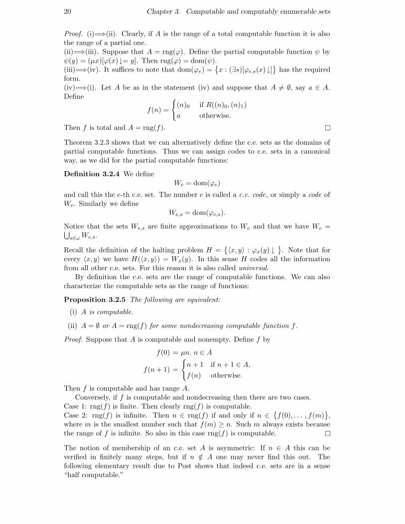
Proof. (i)=⇒(ii). Clearly, if A is the range of a total computable function it is alsothe range of a partial one.(ii)=⇒(iii). Suppose that A = rng(ϕ). Define the partial computable function ψ byψ(y) = (µx)[ϕ(x)↓= y]. Then rng(ϕ) = dom(ψ).(iii)=⇒(iv). It suffices to note that dom(ϕe) =

{x : (∃s)[ϕe,s(x)↓]

}has the required

form.(iv)=⇒(i). Let A be as in the statement (iv) and suppose that A 6= ∅, say a ∈ A.Define

f(n) =

{(n)0 if R((n)0, (n)1)

a otherwise.

Then f is total and A = rng(f). �

Theorem 3.2.3 shows that we can alternatively define the c.e. sets as the domains ofpartial computable functions. Thus we can assign codes to c.e. sets in a canonicalway, as we did for the partial computable functions:

Definition 3.2.4 We defineWe = dom(ϕe)

and call this the e-th c.e. set. The number e is called a c.e. code, or simply a code ofWe. Similarly we define

We,s = dom(ϕe,s).

Notice that the sets We,s are finite approximations to We and that we have We =⋃s∈ωWe,s.

Recall the definition of the halting problem H ={〈x, y〉 : ϕx(y) ↓

}. Note that for

every 〈x, y〉 we have H(〈x, y〉) = Wx(y). In this sense H codes all the informationfrom all other c.e. sets. For this reason it is also called universal.

By definition the c.e. sets are the range of computable functions. We can alsocharacterize the computable sets as the range of functions:

Proposition 3.2.5 The following are equivalent:

(i) A is computable.

(ii) A = ∅ or A = rng(f) for some nondecreasing computable function f .

Proof. Suppose that A is computable and nonempty. Define f by

f(0) = µn. n ∈ A

f(n+ 1) =

{n+ 1 if n+ 1 ∈ A,

f(n) otherwise.

Then f is computable and has range A.Conversely, if f is computable and nondecreasing then there are two cases.

Case 1: rng(f) is finite. Then clearly rng(f) is computable.Case 2: rng(f) is infinite. Then n ∈ rng(f) if and only if n ∈

{f(0), . . . , f(m)

},

where m is the smallest number such that f(m) ≥ n. Such m always exists becausethe range of f is infinite. So also in this case rng(f) is computable. �

The notion of membership of an c.e. set A is asymmetric: If n ∈ A this can beverified in finitely many steps, but if n /∈ A one may never find this out. Thefollowing elementary result due to Post shows that indeed c.e. sets are in a sense“half computable.”

3.3. Undecidable sets 21

Proposition 3.2.6 A set A is computable if and only if both A and its complementA are c.e.

Proof. Informally: To decide wether x ∈ A, enumerate A and A until x appears inone of them. For a formal proof see Exercise 3.8.1. �

3.3 Undecidable sets

We have called a set A computable if its characteristic function χA is computable. Aset A for which we are interested to know for every n whether n ∈ A or n /∈ A is alsocalled a decision problem, depending on the context. A decision problem A that iscomputable is usually called decidable. Note that the halting problem H is a decisionproblem.

Theorem 3.3.1 (Undecidability of the halting problem, Turing [29]) H is undecid-able.

Proof. If H would be decidable then so would K since x ∈ K ⇔ 〈x, x〉 ∈ H. Soit suffices to show that K is undecidable. Suppose for a contradiction that K isdecidable. Then also its complement K is decidable, and in particular c.e. But thenK = We for some code e. Now

e ∈ K ⇐⇒ ϕe(e)↓⇐⇒ e ∈We ⇐⇒ e ∈ K,

a contradiction. �

Theorem 3.3.1 shows that there are c.e. sets that are not computable. The proof thatK is undecidable is yet another example of the diagonalization method.

A natural property for a set of codes is to require that is is closed under functionalequivalence of codes:

Definition 3.3.2 A set A is called an index set if

(∀d, e)[d ∈ A ∧ ϕe = ϕd → e ∈ A].

Notice that H and K are index sets. All sets of codes that are defined by propertiesof the functions are index sets. For example the following sets are all index sets:

• Fin ={e : We is finite

}.

• Tot ={e : ϕe is total

}.

• Comp ={e : We is computable

}.

All of these examples are important, and we will encounter them again in Chapter 4.After seeing that K is undecidable it will not come as a surprise that Fin, Tot,

and Comp are also undecidable, since the task to decide whether a code e is a memberof any of these sets seems harder than just deciding whether it converges on a giveninput. But in fact, the undecidability of these sets follows from a very general resultthat says that essentially all index sets are undecidable:

Theorem 3.3.3 (Rice’s Theorem) Let A be an index set such that A 6= ∅ and A 6= ω.Then A is undecidable.

22 Chapter 3. Computable and computably enumerable sets

Proof. Let A be as in the statement of the theorem. Suppose that e is a code of theeverywhere undefined function, and suppose that e ∈ A. Let d ∈ A and let f be acomputable function such that

ϕf(x) =

{ϕd if x ∈ K,↑ otherwise.

Thenx ∈ K =⇒ ϕf(x) = ϕd =⇒ f(x) /∈ A,

x /∈ K =⇒ ϕf(x) = ϕe =⇒ f(x) ∈ A.

Now if A would be decidable then so would K, contradicting Theorem 3.3.1. Thecase e /∈ A is completely symmetric, now choosing d ∈ A. �

By Rice’s Theorem the only decidable examples of index sets are ∅ and ω. So we seethat undecidability is indeed ubiquitous in computer science.

By Proposition 3.2.6 a set A is computable if and only if both A and A are c.e.We now consider disjoint sets of pairs of c.e. sets in general:

Definition 3.3.4 A disjoint pair of c.e. sets A and B is called computably separableif there is a computable set C such that A ⊆ C and B ⊆ C. A and B are calledcomputably inseparable if they are not computably separable.

Note that the two halves of a computably inseparable pair are necessarily noncom-putable. So the next theorem is a strong form of the existence of noncomputable c.e.sets.

Theorem 3.3.5 There exists a pair of computably inseparable c.e. sets.

Proof. Define

A ={x : ϕx(x)↓= 0

},

B ={x : ϕx(x)↓= 1

}.

Suppose that there is a computable set C separating A and B. Let e be a code ofthe characteristic function of C: ϕe = χC . Then we obtain a contradiction when wewonder whether e ∈ C:

e ∈ C =⇒ ϕe(e) = 1 =⇒ e ∈ B =⇒ e /∈ C,e /∈ C =⇒ ϕe(e) = 0 =⇒ e ∈ A =⇒ e ∈ C. �

Computably inseparable pairs actually do occur in “nature”. E.g. it can be shownthat for formal systems F that are strong enough (at least expressible as arithmetic)the sets of provably true and provably false formulas are computably inseparable.(The proof consists of formalizing the above argument in F .)

3.4 Uniformity

In Theorem 3.2.3 we proved that various ways of defining c.e. sets are equivalent. Butin fact some of these equivalences hold in a stronger form than was actually stated, ascan be seen by looking at the proof. Consider for example the direction (ii)=⇒(iii).The function ψ there was defined in a computable way from the given function ϕ,which means that there is a computable function h such that, if e is a given code for

3.4. Uniformity 23

ϕ, h(e) is a code of ψ. We will say that the implication (ii)=⇒(iii) holds uniformly ,or uniform in codes. In fact one can show that the equivalences of (ii), (iii), and (iv)are all uniform in codes (cf. Exercise 3.8.2).

With respect to the implication (iv)=⇒(i), note that in the proof we distinguishedbetween the cases A = ∅ and A 6= ∅. Now the set

{e : We = ∅

}

is an index set, and hence by Theorem 3.3.3 undecidable. So we cannot effectivelydiscriminate between the two different cases. However we have uniformity in thefollowing form:

Proposition 3.4.1 There is a computable function f such that for every e,

We 6= ∅ =⇒ ϕf(e) total ∧ rng(ϕf(e)) = We.

Proof. Let d be a code such that

ϕd(e, s) =

{m if m ∈We,s+1 −We,s,

µn. n ∈We otherwise.

Define f(e) = S11(d, e). Then f is total since S1

1 is, and when We is nonempty, ϕf(e)

is total with range We. �

As an example of a result that does not hold uniformly we consider the following. Notethat there are two ways to present a finite set: We can present it by its canonical codeas Dn for some n (see Section 2.4.4), i.e. provide a complete list of all its elements,or we can present it by a c.e.-code as We for some e, i.e. provide only an enumerationof its elements. Now we have:

Proposition 3.4.2 We can go effectively from canonical codes to c.e. codes, but notvice versa.

Proof. By the S-m-n theorem, and by the definition of Dn, it is clear that we candefine a computable function f such that Wf(n) = Dn.

Now suppose that we could go from c.e. codes to canonical codes, i.e. supposethat there is a partial computable function ψ such that

We finite =⇒ ψ(e)↓ ∧We = Dψ(e).

Define a computable function g such that

Wg(e) =

{{e} if e ∈ K

∅ otherwise.

Then Wg(e) is always finite, so ψ(g(e))↓ for every e. But then we have

e ∈ K ⇐⇒Wg(e) 6= ∅ ⇐⇒ Dψ(g(e)) 6= ∅.

But Dn = ∅ is decidable, so it follows that K is decidable, contradiction. Hence ψdoes not exist. �

In Proposition 3.7.2 we will use the recursion theorem to show that Proposition 3.2.5also does not hold uniformly.

24 Chapter 3. Computable and computably enumerable sets

3.5 Many-one reducibility

When considering decision problems, or any other kind of problem for that matter,it is useful to have a means of reducing one problem to another. If one can solvea problem A, and problem B reduces to A, then we can also solve B. This alsoworks the other way round: If we know that B is unsolvable, then so must be A. Inthe following we will encounter several notions of reduction. The simplest notion ofreduction between decision problems is maybe the one where questions of the form“n ∈ A?” are effectively transformed into questions of the form “f(n) ∈ B?”, as inthe following definition. A much more general notion will be studied in Chapter 5.

Definition 3.5.1 A set A many-one reduces to a set B, denoted by A ≤m B, if thereis a computable function f such that

n ∈ A⇐⇒ f(n) ∈ B

for every n. The function f is called a many-one reduction, or simply an m-reduction,because it can be noninjective, so that it can potentially reduce many questions aboutmembership in A to one such question about B. We say that A is m-equivalent toB, denoted A ≡m B, if both A ≤m B and B ≤m A. Clearly the relation ≡m isan equivalence relation, and its equivalence classes are called many-one degrees, orsimply m-degrees.

Note that all computable sets have the same m-degree. This is at the same time thesmallest m-degree, since the computable sets m-reduce to any other set.

In the proof of Theorem 3.3.3 we showed that A was noncomputable by actuallybuilding an m-reduction from K to A. That is, we used the following observation:

Proposition 3.5.2 If B is noncomputable and B ≤m A then also A is noncom-putable.

Proof. Trivial. �

Proposition 3.5.3 A set A is c.e. if and only if A ≤m K.

Proof. (If) Suppose that x ∈ A ⇔ f(x) ∈ K for f computable. Then A ={x :

(∃s)[f(x) ∈ Ks]}, where Ks is the finite s-step approximation of K. So by Theo-

rem 3.2.3 A is c.e.

(Only if) Using the S-m-n theorem we define f computable such that

ϕf(e,x)(z) =

{0 if x ∈We,

↑ otherwise.

Then for every e and x, x ∈ We ⇔ ϕf(e,x)(f(e, x)) ↓ ⇔ f(e, x) ∈ K. In particularWe ≤m K for every e. �

An element of a class for which every element of the class reduces to it (under somegiven notion of reduction) is called complete. Proposition 3.5.3 shows that K ism-complete for the c.e. sets. It immediately follows that the halting set H is also m-complete. This we basically saw already on page 20 when we discussed its universality.

By counting we can see that there are many m-degrees:

3.6. Simple sets 25

Proposition 3.5.4 There are 2ℵ0 many m-degrees.

Proof. Note that for every A there are only ℵ0 many B such that B ≤m A since thereare only countable many possible computable functions that can act as m-reduction.In particular every m-degree contains only ℵ0 many sets. (Cf. also Exercise 3.8.7.)Since there are 2ℵ0 many sets the proposition follows. �

3.6 Simple sets

Up to now we have seen two kinds of c.e. set: computable ones and m-complete ones.A very natural question is whether there are any other ones. That is, we ask whetherthere exists a c.e. set that is neither computable nor m-complete. The existence ofsuch sets was shown by Post, and he proved this by considering sets that have a very“thin” complement, in the sense that it is impossible to effectively produce an infinitesubset of their complement. We first note that no c.e. set is itself thin in this sense:

Proposition 3.6.1 (Post [20]) Every infinite c.e. set has an infinite computable sub-set.

Proof. Exercise 3.8.4 �

Definition 3.6.2 A set is immune if it is infinite and it does not contain any infinitec.e. subset. A set A is simple if A is c.e. and its complement A is immune.

Proposition 3.6.3 (Post [20]) If a set is m-complete then it is not simple.

Proof. First we prove that K is not simple. Notice that for every x we have that

Wx ⊆ K =⇒ x ∈ K −Wx (3.1)

because if x ∈ Wx then x ∈ K, and thus Wx 6⊆ K. We can use (3.1) to generate aninfinite c.e. subset of K as follows: Let f be a computable function such that for all x

Wf(x) = Wx ∪ {x}.

Now start with a code x such that Wx = ∅ and repeatedly apply f to obtain theinfinite c.e. set V =

{x, f(x), f(f(x)), . . . , f (n)(x), . . .

}By (3.1), V ⊆ K and V is

infinite. So K contains an infinite c.e. subset, and hence is not simple.Next we prove that if K ≤m A, then the property that K is not simple transfers

to A. Suppose that K ≤m A via h. Let U be a c.e. subset of A. Then the inverseimage h−1(U) is a c.e. subset of K. Moreover, we can effectively obtain a code ofh−1(U) from a code of U . Using the procedure for K above we obtain an elementx ∈ K − h−1(U), and hence h(x) ∈ A − U . By iteration we obtain an infinite c.e.subset of A. Formally: Let g(0) = h(x) whereWx = ∅. Note that g(0) ∈ A. Given theelements g(0), . . . , g(n) ∈ A, let σ(n) be a code of the c.e. set h−1({g(0), . . . , g(n)}).Then by (3.1) σ(n) ∈ K − h−1({g(0), . . . , g(n)}) so we define g(n + 1) = h(σ(n)).Now clearly rng(g) is an infinite c.e. subset of A, and hence A is not simple. �

Theorem 3.6.4 (Post [20]) There exists a simple set.

Proof. We want to build a coinfinite c.e. set A such that for every e the followingrequirement is satisfied:

26 Chapter 3. Computable and computably enumerable sets

Re : We infinite =⇒ A ∩We 6= ∅.

Now we can effectively list all c.e. sets, but we cannot decide which ones are infiniteby the results of Section 3.3. But given a We, we can just wait and see what happenswith it, and enumerate an element from it when we see one that is big enough. Moreprecisely, to keep A infinite we want to make sure that at most e elements from{0, . . . , 2e} go into A. Since we can satisfy Re by just enumerating one element, itsuffices to allow Re to enumerate an element x only if x > 2e. Thus we build the setA in stages as follows:Stage s = 0. Let A0 = ∅.Stage s+ 1. At this stage we are given the current approximation As to A. Look forthe smallest e < s such that As ∩We,s = ∅ and such that there exists an x ∈ We,s

with x > 2e. If such e and x are found, enumerate x into A, i.e. set As+1 = As∪{x}.If such e and x are not found do nothing, i.e. set As+1 = As. This concludes theconstruction.

Now the constructed set A =⋃s∈ω As is infinite because only half of the elements

smaller than 2e can be enumerated into it. Moreover, if We is infinite it contains anx > 2e, which means that some element from We is enumerated into A at some stage.So the requirement Re is satisfied for every e. �

The proof of Theorem 3.6.4 exhibits several features that are typical in computabilitytheory. First notice that it is a diagonalization argument: The overall requirementthat the set should neither be computable nor complete is broken up into infinitelymany subrequirements Re. We then construct a set A that satisfies all of theserequirements in infinitely many stages. An important difference with the examplesfrom Section 3.1 like Cantors argument is that here we cannot take care of requirementRe at stage e, because the construction has to be effective in order to make A c.e.Thus, instead of trying to handle the requirements in order we take a more dynamicapproach, and just wait until we see that a possible action can be taken. Second,there is a mild but decided tension between the requirements Re that want to putelements into A, and are thus of a positive nature, and the overall requirement thatA should be coinfinite, which tries to keep elements out of A, and hence is negative innature. This conflict in requirements was easily solved in this case by restraining theRe from enumerating numbers that are too small. In general the conflicts betweenrequirements in a diagonalization argument may be of a more serious nature, givingrise to more and more complicated methods to resolve them.

Combining the results of this section we obtain:

Corollary 3.6.5 There exists a c.e. set that is neither computable nor m-complete.

In Section 7.3 we will see a natural example of such a c.e. set of intermediate m-degree.

3.7 The recursion theorem

The following theorem is also sometimes called the fixed-point theorem. It has astrong self-referential flavour, and the short and deceptively simple proof does notseem to explain much of the mystery.

Theorem 3.7.1 (The Recursion Theorem, Kleene [11]) For every computable func-tion f there exists an e (called a fixed-point of f) such that ϕf(e) = ϕe.

3.7. The recursion theorem 27

m b

n ϕϕn(m)

diagonal

f

��

ϕϕx(x)

b ϕf◦ϕx(x) ϕϕb(b) = ϕf◦ϕb(b)

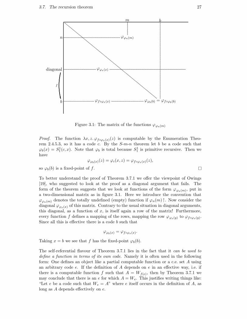
Figure 3.1: The matrix of the functions ϕϕn(m)

Proof. The function λx, z. ϕf◦ϕx(x)(z) is computable by the Enumeration Theo-rem 2.4.5.3, so it has a code c. By the S-m-n theorem let b be a code such thatϕb(x) = S1

1(c, x). Note that ϕb is total because S11 is primitive recursive. Then we

haveϕϕb(x)(z) = ϕc(x, z) = ϕf◦ϕx(x)(z),

so ϕb(b) is a fixed-point of f . �

To better understand the proof of Theorem 3.7.1 we offer the viewpoint of Owings[19], who suggested to look at the proof as a diagonal argument that fails. Theform of the theorem suggests that we look at functions of the form ϕϕn(m), put ina two-dimensional matrix as in figure 3.1. Here we introduce the convention thatϕϕn(m) denotes the totally undefined (empty) function if ϕn(m)↑. Now consider thediagonal ϕϕx(x) of this matrix. Contrary to the usual situation in diagonal arguments,this diagonal, as a function of x, is itself again a row of the matrix! Furthermore,every function f defines a mapping of the rows, mapping the row ϕϕx(y) to ϕf◦ϕx(y).Since all this is effective there is a code b such that

ϕϕb(x) = ϕf◦ϕx(x).

Taking x = b we see that f has the fixed-point ϕb(b).

The self-referential flavour of Theorem 3.7.1 lies in the fact that it can be used todefine a function in terms of its own code. Namely it is often used in the followingform: One defines an object like a partial computable function or a c.e. set A usingan arbitrary code e. If the definition of A depends on e in an effective way, i.e. ifthere is a computable function f such that A = Wf(e), then by Theorem 3.7.1 wemay conclude that there is an e for which A = We. This justifies writing things like:“Let e be a code such that We = A” where e itself occurs in the definition of A, aslong as A depends effectively on e.

28 Chapter 3. Computable and computably enumerable sets

A consequence of Theorem 3.7.1 is the existence of programs that print themselveswhen they are run. Formally, by the S-m-n Theorem 2.4.7 let f be a computablefunction such that for every x, ϕf(e)(x) = e. By Theorem 3.7.1 there is a fixed pointe for which holds that ϕe(x) = e for every x, i.e. the program e prints itself on anyinput.

As another paradoxical example, Theorem 3.7.1 implies the existence of an e suchthat ϕe(x) = ϕe(x) + 1 for every x. But of course the way out of this paradoxicalsituation is that ϕe can be everywhere undefined, which reminds us of the importanceof the fact that we are working with partial functions.

In the next proposition we apply the recursion theorem to show that Proposi-tion 3.2.5 does not hold uniformly.

Proposition 3.7.2 There does not exist a partial computable function ψ such thatfor every e, if ϕe is nondecreasing then ψ(e)↓ and ϕψ(e) = χrng(ϕe).

Proof. Suppose that such ψ does exist, and let ψs denote the s-step approximationof ψ. By the recursion theorem, let e be a code such that

{e}(s) =

{1 if ψs(e)↓ and ϕψ(e),s(1)↓= 0,

0 otherwise.

Then {e} is nondecreasing, so ψ(e) must be defined and ϕψ(e) is total. Now eitherϕψ(e)(1) = 1, in which case rng({e}) contains only 0, or ϕψ(e)(1) = 0, in which case1 ∈ rng({e}). In both cases ϕψ(e)(1) 6= rng({e})(1). �

3.8 Exercises

Exercise 3.8.1 Give a formal proof of Proposition 3.2.6.

Exercise 3.8.2 Prove that the equivalences of (ii), (iii), and (iv) in Theorem 3.2.3are all uniform in codes.

Exercise 3.8.3 The join A⊕B of two sets A and B is defined as

A⊕B ={2x : x ∈ A

}∪{2x+ 1 : x ∈ B

}.

The A ⊕ B contains precisely all the information from A and B “zipped” together.Prove that for every C, if both A ≤m C and B ≤m C then A⊕B ≤m C. Since clearlyA, B ≤m A⊕B this shows that on the m-degrees ⊕ gives the least upper bound of Aand B.

Exercise 3.8.4 Prove Proposition 3.6.1. (Hint: Proposition 3.2.5.)

Exercise 3.8.5 (Reduction Property) Show that for any two c.e. sets A and B thereare c.e. sets A′ ⊆ A and B′ ⊆ B such that A′ ∩B′ = ∅ and A′ ∪B′ = A ∪B.

Exercise 3.8.6 Prove that K and H have the same m-degree.

Exercise 3.8.7 In the proof of Proposition 3.5.4 it was shown that every m-degreecontains at most ℵ0 many sets. Show that also every m-degree contains at least ℵ0

many sets.

3.8. Exercises 29

Exercise 3.8.8 Show that the intersection of two simple sets is again simple. Proveor disprove: The union of two simple sets is again simple.

Exercise 3.8.9 Use the recursion theorem to show that the following exist:

• An e such that We = {e}.

• An e such that for every x, ϕe(x)↓⇐⇒ ϕ2e(x)↓.

• An e such that We = De, where Dn is the canonical listing of all finite sets fromSection 2.4.4.

Exercise 3.8.10 A computable function f is self-describing if e = (µx)[f(x) 6= 0]exists and ϕe = f . Show that self-describing functions exist.

Chapter 4

The arithmetical hierarchy

In Chapter 3 we introduced m-reducibility as a tool to study decidability. But we canalso view m-degrees as a measure for the degree of unsolvability of sets and functions.In Section 3.6 we saw by counting that there are 2ℵ0 many m-degrees, and also thatthere are more than two c.e. m-degrees. (A degree is called c.e. if it contains a c.e.set.) This suggests to classify various classes of sets from mathematics and computerscience according to their m-degree. This is precisely what we do in this chapter. Itturns out that for many naturally defined classes there is moreover a nice relationwith the complexity of their defining formulas. So we start out by defining a hierarchybased on this idea.

4.1 The arithmetical hierarchy

Many sets of natural numbers from mathematics and computer science can be definedby a formula in the language of arithmetic L. Usually, this language is taken to bethe language of the standard model of arithmetic 〈ω, S,+, ·〉, i.e. the natural numberswith successor, plus, and times. We have already seen that by arithmetization we canrepresent all computable functions in this model, so there is no harm in extending thelanguage L with symbols for every computable predicate. Let us call this extension L∗.We also assume that L∗ contains constants to denote every element of ω. For easeof notation we denote the constant denoting the number n also by n. The intendedmodel for L∗ are the natural numbers with all the computable relations, which wedenote again by ω. Thus by ω |= ϕ we denote that the formula ϕ is true in thismodel.

Definition 4.1.1 An n-ary relation R is arithmetical if it is definable by an arith-metical formula, i.e. if there is an L∗-formula ϕ such that for all x1, . . . , xn,

R(x1, . . . , xn) ⇐⇒ ω |= ϕ(x1, . . . , xn).

We can write every L∗-formula ϕ in prenex normal form, i.e. with all quantifiers infront (the prefix of ϕ) and quantifying over a propositional combination of computablepredicates (the matrix of ϕ). Now the idea is that we distinguish defining formulasby their quantifier complexity. First note that two consecutive quantifiers of the samekind can be contracted into one, using coding of pairs. E.g. if ϕ has the form

. . . ∃x∃y . . . R(. . . x . . . y . . . )

then ϕ can be transformed into the equivalent formula

. . . ∃z . . . R(. . . (z)0 . . . (z)1 . . . ).

30

4.1. The arithmetical hierarchy 31

The same holds for consecutive blocks of universal quantifiers. So we will measurequantifier complexity by only counting alternations in quantifiers.

Definition 4.1.2 (The Arithmetical Hierarchy) We inductively define a hierarchy asfollows.

• Σ00 = Π0

0 = the class of all computable relations.

• Σ0n+1 is the class of all relations definable by a formula of the form ∃xR(x, ~y)

where R is a Π0n-predicate.

• Π0n+1 is the class of all relations definable by a formula of the form ∀xR(x, ~y)

where R is a Σ0n-predicate.

• ∆0n = Σ0

n ∩ Π0n for every n.

So Σ0n is the class of relations definable by an L∗-formula in prenex normal form with

n quantifier alternations, and starting with an existential quantifier. Idem for Π0n,

but now starting with a universal quantifier. It follows from Proposition 3.2.6 that∆0

1 consists precisely of all the computable relations, and from Theorem 3.2.3 thatΣ0

1 consists of the c.e. relations. The superscript 0 in the notation for the classes inthe arithmetical hierarchy refers to the fact that they are defined using first-orderformulas, that is formulas with quantification only over numbers. There are indeedhigher order versions defined using more complex formulas, but we will not treat thesehere. For example, the classes of the analytical hierarchy, denoted with a superscript1, are defined using second-oder quantification, where quantifiers are also allowed torun over sets of natural numbers.

Proposition 4.1.3 (Closure properties)

1. R ∈ Σ0n if and only if ¬R ∈ Π0

n.

2. Σ0n, Π0

n, and ∆0n are closed under conjunction, disjunction, and bounded quan-

tification.

3. ∆0n is closed under negations.

4. For n ≥ 1, Σ0n is closed under existential quantification, and Π0

n is closed underuniversal quantification.

Proof. Item (1) follows from the standard procedure of pulling negations throughquantifiers. For items (2) and (3) see Exercise 4.3.1. Item (4) follow from the con-traction of quantifiers discussed on page 30. �

The next theorem shows that our hierarchy does not collapse, and is strict at alllevels.

Theorem 4.1.4 (Hierarchy Theorem) For every n ≥ 1 the following hold:

1. Σ0n − Π0

n 6= ∅, and hence ∆0n ( Σ0

n.

2. Π0n − Σ0

n 6= ∅, and hence ∆0n ( Π0

n.

3. Σ0n ∪ Π0

n ( ∆0n+1.

32 Chapter 4. The arithmetical hierarchy

...

∆0n+1

Σ0n

zzzzzzz

Π0n

DDDDDDD

∆0n

yyyyyyy

DDDDDDD

...

∆03

Σ02

zzzzzzz

Π02

DDDDDDD

∆02

zzzzzzz

DDDDDDD

Σ01

zzzzzzz

Π01

DDDDDDD

∆01

zzzzzzz

DDDDDDD

Figure 4.1: The Arithmetical Hierarchy

Proof. We define analogues Kn of the diagonal set K for every level Σ0n, and we

imitate the proof of Theorem 3.3.1 to show that Kn is not in Π0n. Define

K2n ={e : ∃x1∀x2 . . . ∃x2n−1∀s ϕ2n

e,s(e, x1, . . . , x2n−1)↑},

K2n+1 ={e : ∃x1∀x2 . . . ∀x2n∃s ϕ2n+1

e,s (e, x1, . . . , x2n)↓}.

Clearly Kn ∈ Σ0n for every n. Also note that K1 = K. Now suppose that Kn ∈ Π0

n.Then Kn ∈ Σ0

n, so Kn ={z : ∃x1∀x2 . . . ∃xn R(z, x1, . . . , xn)

}for some com-

putable predicate R. Now by Theorem 3.2.3 there is a code e such that for everyz, x1, . . . , xn−1

∃xn R(z, x1, . . . , xn) ⇐⇒ ∃s ϕe,s(z, x1, . . . , xn)↓ .

Now we obtain a contradiction by considering z = e:

e ∈ Kn ⇐⇒ ∃x1∀x2 . . . ∃xn R(e, x1, . . . , xn)

⇐⇒ ∃x1∀x2 . . . ∀xn−1∃s ϕe,s(z, x1, . . . , xn)↓⇐⇒ e ∈ Kn.

Hence Kn /∈ Π0n. Item (2) immediately follows from this, since Kn ∈ Π0

n − Σ0n.

4.2. Computing levels in the arithmetical hierarchy 33

For item (3) consider the predicate R defined by

R(e, i) ⇐⇒[e ∈ Kn ∧ i = 0

]∨[e ∈ Kn ∧ i = 1

].

This predicate is not in Π0n, for otherwise also R′(e) = R(e, 0) would be Π0

n. ButR′(e) is just Kn, and this is not Π0

n as we have just seen. The same reasoning showsthat R is not Σ0

n. However, it is easy to check that R is both Σ0n+1 and Π0

n+1. SoR ∈ ∆0

n+1 − (Σ0n ∪ Π0

n). �

For the sets Kn from the proof of Theorem 4.1.4 we can actually show more, namelythat they are m-complete at their respective levels:

Proposition 4.1.5 Kn is m-complete for Σ0n.

Proof. Consider any Σ0n set A =

{e : ∃x1∀x2 . . . ∃xn R(e, x1, . . . , xn)

}. Define a

computable function f such that

ϕnf(e)(z, x1, . . . , xn−1) =

{0 if ∃xn R(e, x1, . . . , xn)

↑ otherwise.

Then

e ∈ A ⇐⇒ ∃x1∀x2 . . . ∃xn R(e, x1, . . . , xn)

⇐⇒ ∃x1∀x2 . . . ∀xn−1∃s ϕnf(e),s(f(e), x1, . . . , xn−1)↓⇐⇒ f(e) ∈ Kn. �

Next we consider a famous application of the arithmetical hierarchy, namely Tarski’stheorem saying that arithmetical truth is itself not an arithmetical notion. Let ϕ 7→pϕq be a primitive recursive coding of L∗-sentences, mapping sentences to numbers.pϕq is called the Godel code of ϕ.

Theorem 4.1.6 (Tarski [28]) The set

{pϕq : ω |= ϕ

}

of true arithmetical formulas is not arithmetical.

Proof. Exercise 4.3.2. �

4.2 Computing levels in the arithmetical hierarchy

Given an arithmetically defined set it is usually easy to establish some upper boundon the level of the set in the arithmetical hierarchy, simply by writing out its defin-ing formula in prenex normal form and counting the quantifier alternations. But ofcourse we often want to know the exact level instead of just an upper bound. Propo-sition 4.1.5 provides us with a method to establish lower bounds, namely if we canshow that Kn ≤m A or Kn then we know that A cannot occur at a lower level. Wenow give a number of examples, of growing complexity, illustrating this method.

Proposition 4.2.1 The set A ={e : We = ∅

}is m-complete for Π0

1.

34 Chapter 4. The arithmetical hierarchy

Proof. Since e ∈ A ⇔ ∀x∀s ϕe,s(x) ↑ we see that A is at most Π01. Theorem 3.3.3

shows us that A is noncomputable, but we can actually show that A is m-completefor Π0

1: Let B = W e be an arbitrary Π01 set. Let f be a computable function such

that

ϕf(e)(x) =

{0 if x ∈We,

↑ otherwise.

Then x ∈ We ⇔ Wf(e) 6= ∅, so B ≤m A via f . Since B was arbitrary this shows thecompleteness of A. �

Proposition 4.2.2 • Fin ={e : We is finite

}is m-complete for Σ0

2.

• Tot ={e : ϕe is total

}is m-complete for Π0

2.

Proof. We leave it to the reader to verify that Fin ∈ Σ02 and Tot ∈ Π0

2 (Exercise 4.3.3).We prove the two items simultaneously by providing one reduction for both of them.Let A =

{e : ∀x∃y R(e, x, y)

}be any Π0

2 set. Define a computable function f suchthat

ϕf(e) =

{0 if (∀x < z)(∃y)[R(e, x, y)],

↑ otherwise.

Thene ∈ A ⇐⇒ ∃x∀y ¬R(e, x, y) ⇐⇒ f(e) ∈ Fin,e ∈ A ⇐⇒ ∀x∃y R(e, x, y) ⇐⇒ f(e) ∈ Tot.

�

Theorem 4.2.3 (Rogers, Mostowski) Comp ={e : We is computable

}is m-comp-

lete for Σ03.

Proof. That Comp is Σ03 is shown in Exercise 4.3.3. Let A =

{e : ∃x∀y∃z R(e, x, y, z)

}

be any Σ03 set. Given e we want to build a c.e. set Wf(e) that is either cofinite (and

hence computable) or simple1 (and hence noncomputable), depending on whethere ∈ A or not. We will enumerate Wf(e) in an effective construction by stages. Then-th element of the complement of Wf(e) will be denoted by asn. So at stage s wehave

Wf(e),s ={as0 < as1 < as2 < . . .

}

We think of the asn as markers moving to ever higher positions. Note that Wf(e) iscoinfinite if and only if every marker eventually comes to a rest, i.e. if an = lims→∞ asnexists for every n. Call x infinitary if ∀y∃z R(e, x, y, z), and call x finitary otherwise.Every time we see evidence that x is infinitary we will enumerate asx into Wf(e). So ifx really is infinitary this will make Wf(e) cofinite. We will let Wf(e) contain a simpleset (which exist by Theorem 3.6.4). Hence Wf(e) will be simple itself if and only if itis coinfinite. The construction is as follows.Stage s = 0. We start with Wf(e) = S, where S is a simple set. (Since we cannotactually enumerate all elements of S in one stage, what we actually mean by this isthat we enumerate all the elements of S into Wf(e) over the construction.) We willkeep a length function l(x, s) monitoring whether x is infinitary. Define l(x, 0) = 0for every x.Stage s+ 1. Define

l(x, s) = maxy<s

(∀y′ < y)(∃z)[R(e, x, y, z)].

1In most textbook proofs Wf(e) is made Turing complete, but we have not treated T-reducibilityat this point yet. Moreover, just making Wf(e) simple greatly simplifies the proof.

4.3. Exercises 35

Let x ≤ s be minimal such that l(x, s+ 1) > l(e, s). If such x is found enumerate asxinto Wf(e), i.e. set Wf(e),s+1 = Wf(e),s ∪ {x}. This concludes the construction.

Now to verify that Wf(e) is what we want we consider the following cases. Firstsuppose that all x are finitary. Then an = lims→∞ asn exists for every n and henceWf(e) is coinfinite. Since Wf(e) also contains the simple set S it is itself simple, andhence noncomputable. Second suppose that there is an x that is infinitary. Thenwe already observed above that Wf(e) is cofinite, and hence computable. Since theconstruction of Wf(e) depends effectively on e the function f is computable, and isthus an m-reduction witnessing that A ≤m Comp. Since A was arbitrary it followsthat Comp is m-complete for Σ0

3. �

The construction in the proof of Theorem 4.2.3 is actually our first example of apriority construction, a method that we will study in more detail in Chapter 6. As acorollary to the proof we have:

Corollary 4.2.4 • The set Cof ={e : We is cofinite

}is m-complete for Σ0

3.

• The set{e : We is simple

}is m-complete for Π0

3.

It so happens that most naturally defined arithmetical sets are m-complete for somelevel of the arithmetical hierarchy, so that the above method works most of the time(although the computations can get rather hairy at higher levels). However, theredo exist natural examples (e.g. from the theory of randomness, cf. Proposition 7.3.3)of arithmetical sets that are not m-complete for any level, so the method does notalways work.

4.3 Exercises

Exercise 4.3.1 Prove items (1) – (4) from Proposition 4.1.3.

Exercise 4.3.2 ? Prove Theorem 4.1.6.

Exercise 4.3.3 Verify the following items:

1. Fin ∈ Σ02.

2. Tot ∈ Π02.

3. Comp ∈ Σ03.

4. Cof ∈ Σ03.

5.{e : We is simple

}∈ Π0

3.

Chapter 5

Relativized computation and Turing

degrees

5.1 Turing reducibility

In Definition 3.5.1 we defined a notion of reduction where, in order to decide whethern ∈ A, we were allowed to ask one question about B, namely whether f(x) ∈ B. Thiscan obviously be generalized to two, three, or finitely many questions about B, in anyprecisely prescribed way. Rather than studying such generalizations of m-reducibilityhere, we immediately jump to one of the most liberal notions of reduction, wherequestions of the form “n ∈ A?” are solved by using any finite amount of informationfrom B, in any computable way. Thus, when reducing A to B, we pretend that all theinformation in B is given, and use this to solve A. To model that B is given we can forexample add its characteristic function χB to the initial functions in Definition 2.2.3:

Definition 5.1.1 (Turing [30]) Let A be any set. The class of partial A-recursivefunctions is the smallest class of functions

1. containing the initial functions and χA,

2. closed under composition, primitive recursion, and µ-recursion.

An A-recursive function is a partial A-recursive function that is total.

Alternatively, we could have defined the class of A-computable functions by usingan extension of the Turing machine model, where the information in A is written onan extra infinite input tape. We can again show the equivalence of this approach toDefinition 5.1.1 using arithmetization, exactly as in Chapter 2. So henceforth, we shallspeak about the A-computable functions, by which we will mean any of the equivalentconcepts so obtained. All the basic results about the computable functions carry overto the A-computable functions. In particular we have a coding as in Theorem 2.4.1,and we can define:

Definition 5.1.2 The e-th partial A-computable function is denoted by ϕAe or {e}A.

Definition 5.1.3 (Post [21]) We say that A is Turing reducible to B, denoted A ≤T

B, if A is B-computable. We say that A and B are T-equivalent , denoted A ≡T B ifboth A ≤T B and B ≤T A. The equivalence classes of ≡T are called Turing degrees,or simply T-degrees.

36

5.2. The jump operator 37

When A ≤T B we will also say that A is computable relative to B. The set B is alsosometimes called an oracle, since the information contained in it is given for free. Thenotion of relative computation is central in computability theory, since it embodieshow one can use information in any computable way. Note that it is indeed moreliberal than many-one reducibility, that is, we have

A ≤m B =⇒ A ≤T B,

as the reader can easily verify (Exercise 5.6.1).

Many notions from computability theory can be relativized to an arbitrary oracleA, i.e. their definitions can be generalized by considering A-computable functionsinstead of computable ones. For example, an A-c.e. set is a set that can be enumer-ated by an A-computable function. Many basic results in computability theory alsorelativize in the sense that they remain true when they are relativized to an arbitraryoracle. For example all of the basic notions and results from Chapter 3 relativize (cf.Exercise 5.6.3).

The following basic observation about relativized computations is fundamental,and expresses that any convergent computation, relativized or not, can use only afinite amount of information in an oracle.

Proposition 5.1.4 (Use Principle) Let A be any oracle and suppose that {e}As (x)↓.Then there is a finite string σ @ A such that {e}σs (x) ↓. In particular {e}Bs (x) ↓ forany B A σ.

Proof. Any convergent computation consists of a finite number of computation steps.Hence only a finite number of bits of A can occur in it. �

If {e}A(x)↓ the maximum number of A that is used in the computation (which existsby Proposition 5.1.4) is called the use of the computation.

5.2 The jump operator

We can also relativize the diagonal halting set K to an arbitrary oracle A, and wedenote the result by A′:

A′ ={x : ϕAx (x)↓

}.

(A′ is pronounced as “A prime”.) Now it is easily verified that the proof of The-orem 3.3.1 relativizes, so that A′ is not an A-computable set. Since we also havethat A ≤m A′ the operator ′ is called the jump operator. Notice that ∅′ = K. (∅′ ispronounced as “zero prime”.) We denote the n-th iterate of the jump of A by A(n).Note that ∅(n) ∈ Σ0

n (Exercise 5.6.4).

The difference between many-one and Turing reducibility can be nicely charac-terized in terms of the arithmetical hierarchy:

Proposition 5.2.1 (i) ∆0n+1 =

{A : A ≤T ∅(n)

}for every n.

(ii) Σ0n =

{A : A ≤m ∅(n)

}for every n.

(iii) Σ0n+1 consists of all the sets that are ∅(n)-c.e., that is, enumerable by a ∅(n)-

computable function.

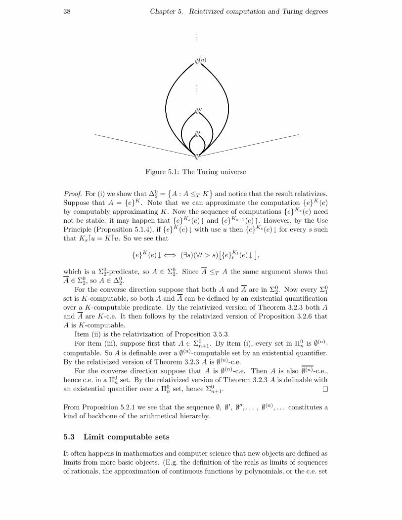
38 Chapter 5. Relativized computation and Turing degrees

...

∅(n)

...

∅′′

∅′

∅

ffffffffffffffffffffffffffffffff

XXXXXXXXXXXXXXXXXXXXXXXXXXXXXXXX

Figure 5.1: The Turing universe

Proof. For (i) we show that ∆02 =

{A : A ≤T K

}and notice that the result relativizes.

Suppose that A = {e}K . Note that we can approximate the computation {e}K(e)by computably approximating K. Now the sequence of computations {e}Ks(e) neednot be stable: it may happen that {e}Ks(e)↓ and {e}Ks+1(e)↑. However, by the UsePrinciple (Proposition 5.1.4), if {e}K(e)↓ with use u then {e}Ks(e)↓ for every s suchthat Ks�u = K�u. So we see that

{e}K(e)↓ ⇐⇒ (∃s)(∀t > s)[{e}Kt

t (e)↓],

which is a Σ02-predicate, so A ∈ Σ0

2. Since A ≤T A the same argument shows thatA ∈ Σ0

2, so A ∈ ∆02.

For the converse direction suppose that both A and A are in Σ02. Now every Σ0

1

set is K-computable, so both A and A can be defined by an existential quantificationover a K-computable predicate. By the relativized version of Theorem 3.2.3 both Aand A are K-c.e. It then follows by the relativized version of Proposition 3.2.6 thatA is K-computable.

Item (ii) is the relativization of Proposition 3.5.3.

For item (iii), suppose first that A ∈ Σ0n+1. By item (i), every set in Π0

n is ∅(n)-

computable. So A is definable over a ∅(n)-computable set by an existential quantifier.By the relativized version of Theorem 3.2.3 A is ∅(n)-c.e.

For the converse direction suppose that A is ∅(n)-c.e. Then A is also ∅(n)-c.e.,hence c.e. in a Π0

n set. By the relativized version of Theorem 3.2.3 A is definable withan existential quantifier over a Π0

n set, hence Σ0n+1. �

From Proposition 5.2.1 we see that the sequence ∅, ∅′, ∅′′, . . . , ∅(n), . . . constitutes akind of backbone of the arithmetical hierarchy.

5.3 Limit computable sets

It often happens in mathematics and computer science that new objects are defined aslimits from more basic objects. (E.g. the definition of the reals as limits of sequencesof rationals, the approximation of continuous functions by polynomials, or the c.e. set

5.4. Incomparable degrees 39

We as the limit of We,s, s ∈ ω.) Here we are interested in the complexity of objectsdefined as the limit of computable processes. Again it turns out that the arithmeticalhierarchy is useful for this purpose.

Definition 5.3.1 A unary function f is limit computable if there is a computablebinary function g such that for all n,

f(n) = lims→∞

g(n, s).

A set A is limit computable if its characteristic function χA is.

Proposition 5.3.2 (Limit Lemma, Shoenfield [25]) A set A is limit computable ifand only if A ∈ ∆0

2.

Proof. (If) We use that ∆02 =

{A : A ≤T K

}(Proposition 5.2.1). Suppose that

A ≤T K, say A = {e}K . Define

g(x, s) =

{{e}Ks

s (x) if {e}Kss (x)↓

0 otherwise.

Now in general the limit lims→∞{e}Kss (x) need not exist, since it may happen that

{e}K(x) ↑ but still {e}Kss (x) ↓ for infinitely many s. But in our case we know that

{e}K( x) ↓ for every x, since it is equal to A(x). So we have that lims g(x, s) = A(x)for every x.

(Only if) Suppose that g is a computable function such that A(x) = lims g(x, s)for every x. Then

x ∈ A ⇐⇒ (∃s)(∀t > s)[g(x, t) = 1]

⇐⇒ (∀s)(∃t > s)[g(x, t) = 1].

So A is both Σ02 and Π0

2, hence ∆02. �

5.4 Incomparable degrees

At this point we have seen that there are more than two c.e. m-degrees, and that ingeneral there are uncountably many m-degrees. The same counting argument thatwe used for m-degrees shows that there are 2ℵ0 many T-degrees (Exercise 5.6.5). Apriori it would be possible that the T-degrees are linearly ordered. In this section weshow that this is not the case. Namely, we show that there are sets A and B suchthat A 6≤T and B 6≤T A. Such sets A and B are called Turing incomparable, and wedenote this by A|TB.

Theorem 5.4.1 (Kleene and Post [12]) There is a pair of Turing incomparable sets.

Proof. We build a pair of incomparable sets A and B by finite extensions, that is, wedefine two series of finite strings σs and τs, s ∈ ω, such that σs @ σs+1, τs @ τs+1, andA =

⋃s∈ω σs and B =

⋃s∈ω τs. The property that A and B should be incomparable

can be split into infinitely many requirements:

R2e : A 6= {e}B ,

40 Chapter 5. Relativized computation and Turing degrees

R2e+1 : B 6= {e}A.

We build A and B in infinitely many stages s, where at stage s = 2e we take care ofR2e and at stage s = 2e+ 1 of R2e+1. We start with σ0 = τ0 = ∅.Stage s = 2e. At this stage σs and τs are already defined, and we define σs+1 andτs+1. To satisfy R2e we need a witness x such that

A(x) 6= {e}B(x). (5.1)

Let x be the smallest number for which A is not yet defined, i.e. let x = |σs|. If theright hand side of (5.1) would be undefined we could take for A(x) whatever we want,and if it were defined we would let A(x) be different from it. First we see if there isany τ w τs such that {e}τ (x) ↓. If such τ does not exist we let A(x) = 0. If such τexists, choose the minimal one (in a fixed computable ordering of all binary strings) oflength greater than x and define τs+1 = τ . Further define σs+1 = σs

(1−{e}τs+1(x)

).

Stage s = 2e + 1. Here we do exactly the same as at stage 2e, except with A and Binterchanged. This completes the construction.

Now first note that⋃s∈ω σs and

⋃s∈ω τs are total, since at every stage they become

defined on a new number x. Second, R2e is satisfied at stage 2e by the choice of σs+1

and τs+1, and similarly for R2e+1. �

The method used in the proof of Theorem 5.4.1 is quite powerful and yields a wealthof information about the structure of the Turing degrees. Arguments where setsare constructed using finite extensions as in the above proof are called Kleene-Postarguments. The proof of Theorem 5.4.1 can be extended to show much more, namelythat there is a set of size 2ℵ0 such that every two of them are mutually incomparable(Exercise 5.6.8). This shows that the Turing universe is as least as wide as it is high.

5.5 Inverting the jump

Since for the jump A′ of any set A we obviously have A′ ≥T ∅′, the range of the jumpoperator is included in the cone

{B : B ≥T ∅′

}. In this section we show, using a

Kleene-Post argument, that the range of the jump operator is in fact equal to thiscone.

Theorem 5.5.1 (Jump Inversion Theorem, Friedberg [6]) The range of the jumpoperator is

{B : B ≥T ∅′

}.

Proof. We show that for every B ≥T ∅′ there is an A such that A′ = B. So let B ≥T ∅′.We define A =

⋃s∈ω σs by finite extensions, as in the proof of Theorem 5.4.1. We

start with σ0 = ∅.Stage s = 2e. At this stage σs is already defined, and we define σs+1. Look if thereis a σ w σs such that

{e}σ(e)↓ .If such σ exists, take the smallest one and define σs+1 = σ.Stage s = 2e+ 1. At this stage we code B into A by setting

σs+1 = σsB(e).

This completes the construction. We verify that A is as we wanted. First note thatthe construction is computable in B: the even stages can be computed by ∅′, and

5.6. Exercises 41

hence by B since ∅′ ≤T B, and the odd stages can be computed by B directly.Second note that the construction is also A ⊕ ∅′-computable, since the even stagesare ∅′-computable, so given ∅′ we can for every e compute σ2e+1 from σ2e and thenwith the help of A compute σ2e+2, hence B(e). So we have

B ≤T A⊕ ∅′ ≤T A′.

The second inequality holds because both A ≤T A′ and ∅′ ≤T A

′. (Cf. Exercise 5.6.2.)Conversely, A′ ≤T A⊕∅′ since to decide whether {e}A(e)↓ we simulate the construc-tion until at stage 2e we can compute whether σ exists. If so, we know we took itso e ∈ A′, and if not then necessarily e /∈ A′. Now we also have A ≤T B since theconstruction is B-computable, as already remarked above. Summarizing we have

A′ ≤T A⊕ ∅′ ≤T B.

Combining this with what we had before we see that A′ ≡T B, as we wanted. �

The proofs of Theorem 5.4.1 and Theorem 5.5.1 are extensions of the diagonalizationmethod discussed at the beginning of Section 3.1. In particular the proof of Theo-rem 5.5.1 contains germs of the method of forcing, which is yet another incarnation ofthe diagonalization method and that has been pushed to great heights in set theory.We will further discuss the power of diagonalization in the next chapter.

5.6 Exercises

Exercise 5.6.1 Verify the following items:

1. A ≤m B =⇒ A ≤T B.

2. A ≤T A.

Exercise 5.6.2 Recall the join operator ⊕ defined in Exercise 3.8.3. Show that ⊕also is a least upper bound operator in the Turing degrees, i.e. prove that for everyC, if both A ≤T C and B ≤T C then A⊕B ≤T C.

Exercise 5.6.3 • Verify that Theorem 3.2.3 relativizes.

• Show that A ≤m A′ and that Theorem 3.3.1 relativizes.

Exercise 5.6.4 Show that ∅(n) is in Σ0n, and that it is m-complete for Σ0

n.

Exercise 5.6.5 Show that every T-degree is countable, and that there are 2ℵ0 manyT-degrees.

Exercise 5.6.6 Show that there is a pair of Turing incomparable sets in ∆02. (Hint:

Show that the construction in the proof of Theorem 5.4.1 is computable in K.)

Exercise 5.6.7 Show that the m-degrees are not linearly ordered. (Hint: Build setsA and B such that for every e the following requirements are satisfied:

R2e : ϕe total =⇒ A 6≤m B via ϕe,

R2e+1 : ϕe total =⇒ B 6≤m A via ϕe.

42 Chapter 5. Relativized computation and Turing degrees

To satisfy R2e, find a witness x such that A(x) 6= B(ϕe(x)). Idem for R2e+1.)

Exercise 5.6.8 ? Show that there is a set of 2ℵ0 many T-degrees that are pairwiseincomparable. (Hint: construct a perfect set, i.e. a subtree of 2ω, such that any twoinfinite paths in it satisfy the requirements of Theorem 5.4.1.)

Exercise 5.6.9 ? A set A is low if the jump of A is as low as possible, namely A′ ≤T ∅′.Let A be a c.e. set and suppose that A has a computable enumeration {As}s∈ω suchthat for all e ∈ ω

(∃∞s)[{e}As

s (e)↓]

=⇒ {e}A(e)↓ .

Prove that then A is low. (Hint: use the Limit Lemma.)

Exercise 5.6.10 (Continuous functionals) A computable functional (also called aTuring functional) F : 2ω → 2ω is a total function of the form F (X)(n) = {e}X (n),that is, the n-th bit of the output is given by the computation {e}X (n). Similarly,an A-computable functional is a total function of the form F (X)(n) = {e}A⊕X (n).

1. Show that every A-computable functional is continuous. (Hint: Use Proposi-tion 5.1.4.)

2. Conversely, show that for every continuous functional F there is an A such thatF is A-computable. (Hint: Let A code the modulus of continuity of F .)

3. Conclude that there are 2ℵ0 continuous functionals.

Chapter 6

The priority method

6.1 Diagonalization, again

In Section 3.1 we discussed the method of diagonalization. Afterwards we encoun-tered the method in several of our fundamental results, such as the undecidability ofthe halting problem (Theorem 3.3.1), the existence of computably inseparable sets(Theorem 3.3.5), the existence of simple sets (Theorem 3.6.4), the recursion theorem(Theorem 3.7.1), and the existence of incomparable Turing degrees (Theorem 5.4.1).

In general, in a diagonal argument one tries to construct an object A with someglobal property P by splitting P into infinitely many subrequirements Re. The objectA is then built using a construction with infinitely many stages. For example, inCantors diagonalization construction A is a set with the global property that it isnot on a given countable list of sets Ai. This property can be split into the infinitelymany subrequirements Ri saying that A 6= Ai for every i. In the construction we cansimply satisfy all Ri in order by defining A(i) = 1 −Ai(i).

After the proof of Theorem 3.6.4 we discussed how it is not always possible tosatisfy the requirements in a diagonalization argument in order, but that due toeffectivity constraints we sometimes have to adopt a more dynamic approach. In thischapter we further generalize the method in order to solve an important questionabout the c.e. Turing degrees.

Apart from the problem that sometimes we cannot effectively see how to satisfya requirement it may happen that the requirements in a diagonalization constructionare in conflict with each other. Note that in Cantors argument the actions taken tosatisfy every requirement do not interfere with each other. However, in Theorem 3.6.4we already saw a conflict between requirements wanting to keep elements out of Aand elements trying to put elements into it. Also in the proof of Theorem 4.2.3there were conflicting requirements, although at that point we did not need to makethis explicit. However, for what follows it will be instructive to explicitly analyzethese requirements. We use the notation from the proof. In the proof we built ac.e. set Wf(e) that was cofinite if an infinitary x existed, and coinfinite otherwise.The requirement that Wf(e) be coinfinite can be split up into the requirements Rx

saying that the marker asx comes to a rest, i.e. that lims→∞ asx is finite for every x.However, if x is infinitary then lims a

sx = ∞ and therefore also lims a

sy = ∞ for every

y > x. That is, the action of enumerating asx is in conflict with Ry. This conflict isresolved by giving the first action priority over the second. Thus, if x is infinitary,every requirement Ry with y > x fails to be satisfied. If on the other hand all x arefinitary every Rx is satisfied.

In general, the priority method is a method for resolving conflicts between re-

43

44 Chapter 6. The priority method

quirements. If in a construction an action taken to satisfy a requirement Ri conflictswith that of a requirement Rj we say that Rj is injured . In this chapter we will onlyconsider constructions were the conflicts between requirements are of a mild nature,namely where every requirement is injured only finitely often. Such arguments arecalled finite injury priority arguments. The finite injury method is significantly morepowerful than the Kleene-Post finite extension method from Chapter 5, and can beused to answer many questions for which the latter fails to provide an answer. In thenext section we discuss the first example of such a question.

6.2 A pair of Turing incomparable c.e. sets

In Theorem 3.6.4 we showed that there are c.e. sets of intermediate m-degree. Afterproving this Post asked the following famous question [20]:

Posts Problem Do there exist c.e. sets of intermediate Turing degree? That is, isthere a c.e. set that is neither computable nor Turing-complete for the c.e. sets?

In Theorem 5.4.1 we showed the existence of a pair of Turing incomparable sets. ByExercise 5.6.6 these such pairs exist also below K. If we would succeed in makingthese sets c.e. we would have settled Posts Problem in the affirmative. This is exactlyhow Friedberg [5] and Muchnik [16] solved the problem, independently of each other.

Theorem 6.2.1 (Solution to Posts Problem, Friedberg [5] and Muchnik [16]) Thereexists a pair of Turing incomparable c.e. sets.

Proof. We build a pair of incomparable c.e. sets A and B, using the same requirementsas in the proof of Theorem 5.4.1: For every e we want to ensure

R2e : A 6= {e}B ,

R2e+1 : B 6= {e}A.

As before, for R2e we need a witness x such that A(x) 6= {e}B(x). We can pick awitness x and initially define A(x) = 0, and wait until {e}Bs

s (x) converges for somes. If this never happens R2e is automatically satisfied. If {e}Bs

s (x)↓= 1 we are done,and if {e}Bs

s (x) ↓= 0 we can enumerate x into A so that A(x) = 1 and again R2e issatisfied. The difference with Theorem 5.4.1 is that here we have no complete controlover the set B. In fact, we know in advance that A and B will be noncomputable,and for a typical noncomputable set one can never know whether maybe later somesmall element will appear in the set (cf. Proposition 3.2.5). Having satisfied R2e asabove, it might happen that R2e1 wants to enumerate some element into B below theuse of the computation {e}Bs

s (x)↓, and thus spoiling it. To resolve such conflicts, wegive the requirements the priority ordering

R0 > R1 > R2 > R3 > . . .

In case of a conflict we allow the highest priority requirement Ri (i.e. the one with thesmallest index i) to proceed, thus possibly injuring lower priority requirements. Onthe other hand, if i < j we will not allow the low priority requirement Rj to injure acomputation of Ri. We now give the formal construction of A and B by describingtheir enumerations As and Bs, s ∈ ω. To monitor the numbers that requirement Re

wants to keep out of A or B we will use a restraint function r(e, s). We will say that

6.3. Exercises 45

a requirement Re is initialized at a stage s when its current witness xe,s is redefinedto a number greater than any number previously used in the construction, and bysetting the restraint r(e, s) to 0. We will say that R2e requires attention at stage sif since the last stage that R2e was initialized no action for it was taken, and for thecurrent witness x2e,s it holds that {e}Bs

s (xe,s)↓. Similarly for R2e+1.Stage s = 0. Let A0 = B0 = ∅. Initialize all requirements by setting xe,0 = e andr(e, 0) = 0 for every e.Stage s + 1. Let e be the minimal number smaller than s such that Re requiresattention. Define

r(e, s+ 1) = use({e}Bs

s (xe,s))

and say that Re acts. Suppose that e is even. If {e}Bss (xe,s) = 0 define As+1(xe,s) = 1.

Since this action may injure lower priority requirements, we initialize all Rj with j > e.The case where e is odd is completely symmetrical, interchanging the role of A andB. This completes the construction.

We verify that all requirements are satisfied. We prove by induction that everyrequirement acts only finitely often, and is only finitely often initialized. Suppose thats is a stage such that no requirement Rj , j < e acts after stage s. Then Re is neverinitialized after stage s, and limt→∞ xe,t = xe,s. If Re never requires attention afterstage s then it is automatically satisfied. If Re requires attention at some stage t ≥ sthen its restraint r(e, t) is set to the use of the computation {e}Bs

s (xe,s) (in case e iseven). Since all Rj with j > e are initialized at stage t, in particular their witnessesare redefined to be greater than r(e, t + 1), so no such requirement can change thiscomputation. Since also no Rj with j < e acts after t the computation is preservedforever, and hence Re is satisfied. So we see that every requirement is initialized onlyfinitely often, and afterwards is satisfied either vacuously or by one additional action,and hence also acts only finitely often. �

6.3 Exercises

Exercise 6.3.1 ? Show that the c.e. m-degrees are not linearly ordered. (Hint: Buildsets A andB as in Exercise 5.6.7, except that now the construction has to be effective.)

Exercise 6.3.2 ? Show that there is a low simple set A. Note that such a set providesanother solution to Posts Problem. (Hint: use the priority method to build A instages. Use the characterization from Exercise 5.6.9 to make A low, and use thestrategy from Theorem 3.6.4 to make A simple.)

Chapter 7

Applications

Computability theory is a standard ingredient in any course in mathematical logic.Although branches like model theory, set theory, and proof theory have developed intoindividual subjects of their own, the ties with computability theory remain numerous,and new ones keep on being found. Besides, with the rise of computer science it hasbecome indispensable as a background theory for this relatively new area. Severalcomputer science topics have stemmed from computability theory, such as complexitytheory, learning theory, and formal language and automata theory. (The latter is builton yet another characterization of the computable sets, namely as those that can begenerated by a grammar.) In many ways various of the above areas do not have aclear separation. E.g. in the view of Odifreddi [17, 18], the areas of complexity andcomputability theory and descriptive set theory are all the same.

In this chapter we briefly indicate three other areas where computability theoryis pivotal, namely proof theory, constructivism, and randomness.

7.1 Undecidability in logic

By a formal system we will mean any c.e. set F of logical formulas. This is of coursea crude version of the notion of formal system usually employed in mathematicsand computer science (with proper axioms and deduction rules and the like) but itwill suffice here and make what follows all the more general. By arithmetizationwe may treat any formal system F as a set of natural numbers (recall the Godelcoding from page 33). In particular, we can speak of F being decidable or not. Therequirement that F is c.e. corresponds to the fact that most natural formal systemshave a computable set of axioms from which all theorems of the system are deduced,so that the set of deduced formulas is c.e. Such systems are also called axiomatizable.If a formula ϕ is enumerated into F we say that F proves ϕ and we call ϕ a theoremof F , and denote this by F ` ϕ. The above definitions apply to formal systems inany logical language, but as in Chapter 4 we will concentrate on formal systems inthe language of arithmetic. Recall that we use ω |= ϕ to denote that an arithmeticalsentence ϕ holds in the standard model of arithmetic.

Some essential properties of a logical system are whether what it proves is true,whether it is consistent, and whether it decides the truth of every formula:

Definition 7.1.1 Let F be a formal system in the language of arithmetic.

• F is sound if F ` ϕ implies that ω |= ϕ.

• F is consistent if there is no formula ϕ such that both ϕ and ¬ϕ belong to F .

46

7.1. Undecidability in logic 47

• F is complete if for every formula ϕ, either F ` ϕ or F ` ¬ϕ. Otherwise F iscalled incomplete.

Proposition 7.1.2 A consistent and complete formal system is decidable.

Proof. This is a form of Proposition 3.2.6. If F is complete we can enumerate thetheorems of F until either ϕ or ¬ϕ appears. By consistency of F at most one canappear, and by completeness at least one will appear. Hence we can compute whetherϕ is a theorem of F or not. �

In the rest of this section we will work with Robinson Arithmetic Q, which containsthe constant 0, the function symbols S, +, and ·, and the following axioms (besidesthe axioms for first-order predicate logic):

A1. S(x) = S(y) → x = y

A2. S(x) 6= 0

A3. x 6= 0 → (∃y)[x = S(y)]

A4. x+ 0 = x

A5. x+ S(y) = S(x+ y)

A6. x · 0 = 0

A7. x · S(y) = x · y + x

Note that the last four axioms are just the recursive relations for + and · we alreadyencountered on page 5. It would be possible to work with systems weaker than Q, butQ will be convenient for our purposes. The system PA of Peano Arithmetic, whichis very often used as a basic system of arithmetic, is obtained from Q by adding to itthe axiom scheme of induction.

A crucial notion is the power that formal systems have to represent functions:

Definition 7.1.3 A function f is representable in a formal system F if there is aformula ϕ such that for all x and y,

f(x) = y ⇐⇒ F ` ϕ(x, y),

f(x) 6= y ⇐⇒ F ` ¬ϕ(x, y).

Here the x and y in ϕ(x, y) are shorthand for the terms Sx(0) and Sy(0).

The following result adds yet another characterization of the notion of computablefunction to our list.

Theorem 7.1.4 Every computable function is representable in Q. Conversely, everyQ-representable function is computable.

Proof. Both directions can be proved using arithmetization (cf. Section 2.4). We willnot prove this here. A proof can be found in Odifreddi [17]. That every representablefunction is computable is a straightforward application of arithmetization. That everycomputable function is representable requires one more idea, namely the eliminationof primitive recursion using coding. This can be done as in the proof of Theorem 2.4.1,

48 Chapter 7. Applications

except that now we cannot use the coding functions from Section 2.4.1 since thesewere defined using primitive recursion. Instead we need to define different codingfunctions not using primitive recursion. Godel [7] defined such a coding function βusing the Chinese Remainder Theorem. �

The following result is Godels celebrated first incompleteness theorem. It showsthat every formal system is either too weak to contain elementary arithmetic, orincomplete.

Theorem 7.1.5 (The First Incompleteness Theorem, Godel [7]) Any consistent for-mal system F extending Q is undecidable and incomplete.

Proof. Let F be as in the theorem, and suppose that F is decidable. Let {ψn}n∈ω bean effective enumeration of all formulas of one variable. Define the diagonal D by

n ∈ D ⇐⇒ F ` ψn(n).

Since F is decidable D is computable, hence by Theorem 7.1.4 it is representable.Say that ψe represents D:

n ∈ D ⇐⇒ F ` ψe(n).

Then for n = e we obtain a contradiction. This shows that F is undecidable. ThatF is incomplete now follows from Proposition 7.1.2. �

For consistent formal systems F extending Q Godel also proved that a specific sen-tence is unprovable in F , namely the sentence ConF expressing the consistency of F .This result is called the second incompleteness theorem.

By Proposition 3.5.3 the set K is Π01-complete. Let F be a sound formal system.

Then it cannot be the case that for every n ∈ K the system F proves that n ∈ K,since then, because the set of theorems of F is c.e. and F is sound, K would be Σ0

1.So we see that there are (in fact infinitely many) sentences of the form n ∈ K thatare true but that F cannot prove.

The next result is the negative solution to the Entscheidungsproblem mentionedon page 3:

Theorem 7.1.6 (The unsolvability of the Entscheidungsproblem, Church [2] andTuring [29]) First-order predicate logic is undecidable.

Proof. We use that Q has a finite axiomatization. Let∧Q be the conjunction of all

axioms of Q. Then we have for any formula ϕ that

Q ` ϕ ⇐⇒ ` ∧Q → ϕ,

where the ` on the right hand side refers to deducibility in first-order logic. Nowif first-order logic would be decidable it would follow that also Q were decidable,contradicting Theorem 7.1.5. �

7.2. Constructivism 49

7.2 Constructivism

In mathematics one can often prove the existence of objects indirectly by showingthat the assumption that they do not exist leads to a contradiction, or by derivingthe existence from a disjunction A ∨ ¬A without knowing which case obtains. Itmay easily happen that one can show the existence of something in this way withouthaving a clue about how to obtain a concrete example. In constructive mathematicsone tries to prove theorems or construct objects in an explicit way. There are differentschools of constructivism, according to the different meanings that can be given to theword “constructive”. The school of intuitionism founded by the Dutch mathematicianL. E. J. Brouwer proceeded by restricting the means of reasoning from classical logic,by for example not allowing indirect forms of reasoning as in the example above.Another important interpretation is to interpret “constructive” by “computable”.The relation between these two approaches to constructivism is an interesting fieldof study in itself, but in this section we will stick to the latter approach and merelyindicate how computability theory can be used to analyze the constructive content oftheorems from classical mathematics. We will discuss only a single example, namelyKonigs Lemma.

Definition 7.2.1 A (binary) tree is a subset T of 2<ω that is closed under the sub-sequence relation v, i.e. if τ v σ and σ ∈ T then also τ ∈ T . A tree is computablesimply if it is computable when coded as a set of numbers (using any computablecoding of 2<ω). A path in T is an infinite branch of the tree, that is a set A ∈ 2ω

such that A�n ∈ T for every n.

Theorem 7.2.2 (Konigs Lemma) Every infinite binary tree has a path.

Proof. Let T be an infinite binary tree. We inductively “construct” a path trough Tas follows. Let σ0 = ∅. Given σn such that the set

{τ ∈ T : τ w σn

}

is infinite, at least one of σn0, σn1 has infinitely many extensions on T . Defineσn+1 = σn0 if this holds for σn0, and define σn+1 = σn1 otherwise. Now clearly⋃n σn is a path in T . �

Konings Lemma holds in more generality for finitely branching trees, i.e. trees that arenot necessarily binary but in which still every node has only finitely many successors.The next result shows that in general Konigs Lemma is not constructive.

Proposition 7.2.3 There is an infinite computable binary tree without a computablepath.

Proof. By Exercise 7.4.3, for any disjoint pair A,B of c.e. sets there is a computabletree such that the paths in T are precisely the sets separating A and B. Taking Aand B a pair of computably inseparable sets (Theorem 3.3.5) we see that T has nocomputable paths. �

Now we want to analyze exactly how difficult it is to compute a path in an infinitetree. The following result shows that having K as an oracle suffices.

Proposition 7.2.4 (Kreisel Basis Lemma) Every infinite computable binary treehas a path in ∆0

2.

50 Chapter 7. Applications

Proof. For a computable tree, the decision in the proof of Theorem 7.2.2 is computablein K. Thus the path constructed there is also K-computable. �

Proposition 7.2.4 can be significantly improved as follows. In Exercise 5.6.9 we intro-duced the low sets as the sets that have the same jump as computable sets. In thissense they are close to computable sets. Note for example that a low set is not Turingcomplete since complete sets jump above ∅′′. Now by Proposition 7.2.3 we cannotexpect a computable tree to have a computable path, but the next result shows wecan get quite close:

Theorem 7.2.5 (Low Basis Theorem, Jockusch and Soare [9]) Every infinite com-putable binary tree has a low path.

Proof. The proof is a magnificent example of the method of tree-forcing. A discussionof this method, however, would carry us too far at this point. A proof can be foundin Odifreddi [17] or Soare [27]. �

We remark that all the results of this section can be relativized by increasing thecomplexity of the tree, so that they are not only about computable trees but reallystate how difficult it is in general to compute paths in any kind of tree.

The preceding sequence of results illustrate how one often can analyze the con-structive content of mathematical theorems using measures and notions from com-putability theory. Notice that we were not only able to conclude that Konigs Lemmais not constructive, but also obtained a precise bound on how nonconstructive it is interms of Turing degrees.

Another field where the strength of mathematical theorems is studied is the areaof reverse mathematics. Although here the main tools of study here are axiomaticcomputability theory also plays an important role. Many other examples such as theone above can be found in the book by Simpson [26].

7.3 Randomness and Kolmogorov complexity

According to classical probability theory every string of a given length n is just asprobable as another. Yet we feel that there are great qualitative differences betweenstrings. E.g. the sequence 000 . . . 0 consisting of 100 zeros appears to us to be specialamong all strings of length 100. This is part of the motivation for introducing acomplexity measure for individual strings and reals. A general introduction to thisarea is Li and Vitanyi [14].

Fix a universal Turing machine U . (That is, a Turing machine that can simulateall other Turing machines. Such machines exist for the same reason that universalc.e. sets exist, cf. page 20.) Given a string σ ∈ 2<ω, define the Kolmogorov complexityof σ as

C(σ) = min{|τ | : U(τ) = σ}.We list some basic facts of C:

• Note that C depends on the choice of the universal machine U . However thechoice of U matters only an additive constant in the theory: For any two uni-versal machines U and V and the corresponding complexity functions CU andCV we have that CV (σ) ≤ CU (σ) + O(1) for every σ, where the constant O(1)depends only on U and V . Since the choice of U does not matter much, we willhenceforth simply write C instead of CU .

7.4. Exercises 51

• Since every string is a description of itself, we have that the complexity of anystring is bounded by its length. That is, for all σ we have

C(σ) ≤ |σ| +O(1).

Now the idea is that a random string is a string that lacks structure that could beused to obtain a short description of it. For example the string 000 . . . 0 consistingof 1000 zeros is quite long but is easy to describe. On the other hand, a sequenceobtained by 1000 coin flips will probably not have a description that is much shorterthan 1000 bits. So we define:

Definition 7.3.1 A string σ is k-random if C(σ) ≥ |σ| − k.

Proposition 7.3.2 For every k there exist k-random strings.

Proof. This can be shown by simple counting: For a given length n, there are

n−k−1∑

i=0

2−i = 2n−k − 1

programs of length < n− k, so there are at least 2n − 2n−k + 1 k-random strings oflength n. �

In Theorem 3.6.4 we constructed a simple set by brute force. The next result showsthat there are also natural examples of simple sets:

Proposition 7.3.3 For any k, the set of non-k-random strings is simple.

Proof. We leave it to the reader to verify that the set of nonrandom strings is c.e.(Exercise 7.4.5.) We have to show that for every k the set of k-random stringsis immune, i.e. does not contain any infinite c.e. subsets. Suppose that it is notimmune. Then for every m we can compute a string ψ(m) with C(ψ(m)) ≥ m. Butthen m ≤ C(ψ(m)) ≤ logm + O(1), which can only be true for finitely many m, acontradiction. �

Corollary 7.3.4 1. C is not a computable function.

2. If m(x) = min{C(y) : y ≥ x} then m is unbounded.

3. m grows slower than any monotone unbounded computable function.

Proof. See Exercise 7.4.6. That m is unbounded is because we run out of shortprograms. That it grows slower than any computable function is because otherwisewe could enumerate infinitely many high-complexity strings, which is impossible byProposition 7.3.3. �

7.4 Exercises

Exercise 7.4.1 Let “e ∈ Tot” abbreviate the formula ∀x∃s {e}s(x) ↓. Let F be asound formal system. Use Proposition 4.2.2 to show that there are e ∈ Tot for whichF 6` e ∈ Tot.

52 Chapter 7. Applications

Exercise 7.4.2 Prove the result of Exercise 7.4.1 by constructing such an e by directdiagonalization. (Hint: Let {e}(x)↓ for every x for which F does not prove in x stepsthat e ∈ Tot. As soon as F proves that e ∈ Tot let {e} be undefined on all furtherarguments.)

Exercise 7.4.3 Let A,B be any pair of disjoint c.e. sets. Show that there is a com-putable tree T such that the sets that are a separation of A and B are precisely thepaths in T .

Exercise 7.4.4 Let F be a formal system. A complete extension of F is any setseparating

{ϕ : F ` ϕ

}and

{ϕ : F ` ¬ϕ

}.

Show that there is a complete extension of F of low degree. (Hint: Use theprevious exercise and the low basis theorem.) For F a strong formal system such asQ or PA this shows that, although the set

{ϕ : F ` ϕ

}is Σ0

1-complete, there isalways a complete extension that has incomplete Turing degree. In general, however,such a low extension cannot be c.e.

Exercise 7.4.5 Show that for any k the set of k-random strings is Π01.

Exercise 7.4.6 Verify the facts of Corollary 7.3.4.

Further reading

The first textbook solely devoted to computability theory was Rogers [22]. Although itis now outdated in several respects, it is still a good read, and perfectly acceptable foruse as an introduction. Another, but much shorter and advanced, early reference thatwas quite influential is Sacks [23]. The monumental two-volume work by Odifreddi [17,18] is the most extensive and broadest treatment of the subject to-day. The numberof topics discussed in this book an the ease of presentation are quite astounding. Theencyclopaedic character of the book may render it less suited for an introduction, butas reference it has become indispensable. Soares book [27] was written as a modernreplacement of Rogers’ book. It is an excellent reference for the more advanced topicsin computability theory, with a focus on the treatment of the c.e. Turing degreesand the priority method. Sacks [24] treats computability theory on ordinals otherthan ω. In Chapter 7 we have already mentioned various references for applicationsof computability theory. An extensive collection of survey papers on computablemathematics can be found in [4]. Numerous other treatments of the subject, oftenin tandem with subjects like complexity- or automata theory, can be found in anymathematics or computer science library. One can of course also always consult theoriginal papers by the pioneers of the subject. In this case these include the ground-breaking papers by Godel [7], Church [2], Kleene [10], Turing [29], and Post [20].

53

Bibliography

[1] G. Cantor, Uber eine Eigenschaft des Inbegriffs aller reellen algebraischen Zahlen,J. Math. 77 (1874) 258–262.

[2] A. Church, A note on the Entscheidungsproblem, Journal of Symbolic Logic 1(1936) 40–41.

[3] R. Dedekind, Was sind und was sollen die Zahlen?, Braunschweig, 1888.

[4] Yu. L. Ershov, S. S. Goncharov, A. Nerode, J.B. Remmel, and V. W. Marek(eds.), Handbook of Recursive Mathematics, Studies in logic and the foundationsof mathematics Vol’s 138 and 139, North-Holland, 1998.

[5] R. M. Friedberg, Two recursively enumerable sets of incomparable degrees ofunsolvability, Proc. Nat. Acad. Sci. 43 (1957) 236–238.

[6] R. M. Friedberg, A criterion for completeness of degrees of unsolvability, Journalof Symbolic Logic 22(1957) 159–160.

[7] K. Godel, Uber formal unentscheidbare Satze der Principia Mathematica undverwandter Systeme I, Monatshefte fur Mathematik und Physik 38 (1931) 173–198.

[8] D. Hilbert, Mathematische Probleme, Proc. Int. Congr. Math. (1900) 58–114.

[9] C. G. Jockusch, Jr. and R. I. Soare, Π01 classes and degrees of theories, Transac-

tions of the American Mathematical Society 173 (1972) 35–56.

[10] S. C. Kleene, General recursive functions of natural numbers, Math. Ann. 112(1936) 727–742.

[11] S. C. Kleene, On notations for ordinal numbers, Journal of Symbolic Logic 3(1938) 150–155.

[12] S. C. Kleene and E. L. Post, The upper semi-lattice of degrees of recursive un-solvability, Annals of Mathematics, Ser. 2, Vol. 59 (1954) 379–407.

[13] G. W. Leibniz, Dissertatio de arte combinatoria, 1666.

[14] M. Li and P. Vitanyi, An introduction to Kolmogorov complexity and its appli-cations, Springer-Verlag, 1993.

[15] Yu. V. Matijasevich, Enumerable sets are diophantine, Dokl. Acad. Nauk. 191(1970) 279–282.

[16] A. A. Muchnik, On the unsolvability of the problem of reducibility in the theoryof algorithms, Dokl. Akad. Nauk SSSR, N.S. 108 (1956) 194–197 (Russian).

54

Bibliography 55

[17] P. G. Odifreddi, Classical recursion theory, Vol. 1, Studies in logic and the foun-dations of mathematics Vol. 125, North-Holland, 1989.

[18] P. G. Odifreddi, Classical recursion theory, Vol. 2, Studies in logic and the foun-dations of mathematics Vol. 143, North-Holland, 1999.

[19] J. C. Owings, Diagonalization and the recursion theorem, Notre Dame Journalof Formal Logic 14 (1973) 95–99.

[20] E. L. Post, Recursively enumerable sets of positive integers and their decisionproblems, Bull. Amer. Math. Soc. 50 (1944) 284–316.

[21] E. L. Post, Degrees of recursive unsolvability, Bull. Amer. Math. Soc. 54 (1948)641–642.

[22] H. Rogers Jr., Theory of recursive functions and effective computability, McGraw-Hill, 1967.

[23] G. E. Sacks, Degrees of unsolvability, Annals of Mathematics Studies 55, Prince-ton University Press, 1963.

[24] G. E. Sacks, Higher recursion theory, Springer Verlag, 1990.

[25] J. R. Shoenfield, On degrees of unsolvability, Annals of Mathematics 69 (1959)644–653.

[26] S. G. Simpson, Subsystems of second-order arithmetic, Springer-Verlag, 1999

[27] R. I. Soare, Recursively enumerable sets and degrees, Springer-Verlag, 1987.

[28] A. Tarski, Der Wahrheitsbegriff in der formalisierten Sprachen, Studia Phil. 1(1936) 261–405.

[29] A. M. Turing, On computable numbers with an application to the Entschei-dungsproblem, Proc. London Math. Soc. 42 (1936) 230–265, corrections ibid.43 (1937) 544–546.

[30] A. M. Turing, Systems of logic based on ordinals, Proc. London Math. Soc. 45(1939) 161–228.

Index

A′, jump of A, 37

A(n), n-th jump of A, 372ω, Cantor space, 22<ω, finite binary strings, 2∆0n, 31

Π0n, 31

Σ0n, 31

F ` ϕ, F proves ϕ, 46pϕq, Godel code of ϕ, 33⊕, join operator, 28, 41≤m, many-one reducibility, 24ω, 2, 30ω |= ϕ, 30〈· , ·〉, pairing function, 10ϕe, {e}, eth partial computable func-

tion, 13ϕAe , {e}A, eth partial A-computable func-

tion, 36πin, projection functions, 5Smn , 14≤T , Turing reducibility, 36∅′, 37

al-Khwarizmi, 3analytical hierarchy, 31arithmetical, 30arithmetical hierarchy, 31arithmetization, 9axiomatizable, 46

Brouwer, 49

C, Kolmogorov complexity function,50

canonical code, 15Cantor, 18, 19, 26c.e., computably enumerable, 18Church, 4, 48, 53Church’s Thesis, 13code, 10, 20Comp, 21, 34complete

extension, 52

formal system, 47set, 24, 33

computable, 8computable in A, 36computably inseparable, 22, 49consistent, 46course-of-values recursion, 16

De, finite set with canonical code e, 15decidable, 21, 46decision problem, 21Dedekind, 4diagonalization, 18, 26, 27, 41, 43

Entscheidungsproblem, 3, 4, 48enumeration theorem, 14

Fibonacci, 4, 15Fin, 21, 34finite injury, 44fixed-point, 26forcing, 41formal system, 46Friedberg, 40, 44functional

A-computable, 42computable, 42

Godel, 4, 9, 48, 53Grassmann, 5

H, halting problem, 19hierarchy theorem, 31Hilberts 10th problem, 3, 4

immune, 25, 51incomparable

c.e. sets, 44, 45sets, 39–42sets below K, 41

incomplete, 47, 48incompleteness theorem

first, 48second, 48

56

Index 57

index set, 21initial functions, 5injury, 44

Jockusch, 50

jump inversion theorem, 40jump operator, 37

K, diagonal set, 19Kn, complete set for Σ0

n, 32Kleene, 6, 10, 26, 39, 53Kleene-Post arguments, 40, 44

Konigs lemma, 49Kolmogorov, 50Kreisel basis lemma, 49

Leibniz, 3, 9limit computable, 39

limit lemma, 39low, 42, 45, 50low basis theorem, 50

Matijasevich, 4m-complete, 24m-degrees, 24

Mostowski, 34m-reduction, 24µ-operator, 5µ-recursion, 6

Muchnik, 44

normal form theorem, 10

Odifreddi, 46, 53

oracle, 37Owings, 27

PA, Peano arithmetic, 47padding lemma, 14partial computable, 7

partial recursive, 6path, 49Peter, 16Post, 20, 25, 36, 39, 44, 53

Posts Problem, 44prenex normal form, 30primitive recursive, 4priority method, 35, 43

Q, Robinson arithmetic, 47

random string, 51

recursion theorem, 26recursive, 6recursive in A, 36relativization, 37representable, 47Rice, 21Rogers, 34, 53

S, successor function, 5Sacks, 53self-reference, 14, 18, 27Shoenfield, 39simple, 25, 45, 51Simpson, 50S-m-n theorem, 14Soare, 50, 53sound, 46

tally representation, 7Tarski, 33Tn, Kleene’s T -predicate, 10Tot, 21, 34tree, 49Turing, iii, 4, 6, 8, 13, 21, 36, 48, 53Turing degrees, 36Turing machine, 7

U , extraction function, 10uniformity, 23, 28universal, 20, 50use, 37use principle, 37

We, eth c.e. set, 20