Page 1/33

Ground Penetrating Radar for BelowgroundPhenotyping of High-biomass Grasses for SoilCarbon SequestrationMatthew Wolfe  ( mwolfe45@gmail.com )

Texas A&M University https://orcid.org/0000-0002-8076-1509Da Huo 

Texas A&M UniversityHenry Ruiz-Guzman 

Texas A&M UniversityBrody Teare 

Texas A&M UniversityTyler Adams 

Texas A&M UniversityIliyana Dobreva 

Texas A&M UniversityMark Everett 

Texas A&M UniversityMichael Bishop 

Texas A&M UniversityRussell Jessup 

Texas A&M UniversityDirk Hays 

Texas A&M University

Research Article

Keywords: Climate change, Carbon sequestration, Root phenotyping

Posted Date: December 1st, 2021

DOI: https://doi.org/10.21203/rs.3.rs-1041672/v1

License: This work is licensed under a Creative Commons Attribution 4.0 International License.  Read Full License

Page 2/33

AbstractAims

Many governments and companies have committed to moving to net-zero emissions by 2030 or 2050 totackle climate change, which require the development of new carbon capture and sequestration/storage(CCS) techniques. A proposed method of sequestration is to deposit carbon in soils as plant matterincluding root mass and root exudates. Adding perennial traits such as rhizomes to crops as part of asequestration strategy would result in annual crop regrowth from rhizome meristems rather than requiringreplanting from seeds which would in turn encourage no-till agricultural practices. Integrating these traitsinto productive agriculture requires a belowground phenotyping method compatible with high throughputbreeding and selection methods (i.e., is rapid, inexpensive, reliable, and non-invasive), however nonecurrently exist.

Methods

Ground penetrating radar (GPR) is a non-invasive subsurface sensing technology that shows potential asa phenotyping technique. In this study, a prototype GPR antenna array was used to scan roots of theperennial sorghum hybrid, PSH09TX15. A-scan level time-domain analyses and B-scan leveltime/frequency analyses using the continuous wavelet transform were utilized to extract features ofinterest from the acquired radargrams.

Results

Of six A-scan diagnostic indices examined, the standard deviation of signal amplitude correlated mostsigni�cantly with belowground biomass. Time frequency analysis using the continuous wavelettransform yielded high correlations of B-scan features with belowground biomass.

Conclusion

These results demonstrate that continued re�nement of GPR data analysis work�ows should yield ahighly applicable phenotyping tool for breeding efforts in environments where selection is otherwiseimpractical on a large scale.

1. IntroductionOngoing climate change due to global temperature increase affects all Earth systems. Global averagetemperature has increased by 0.85°C between 1880 and 2012, and is expected to reach 1.5°C abovepreindustrial temperatures by 2040 (Allen, M.R., O.P. Dube, W. Solecki, F. Aragón-Durand, W. Cramer, S.Humphreys, M. Kainuma, J. Kala, N. Mahowald, Y. Mulugetta, R. Perez, M. Wairiu 2018). Human activityhas helped drive atmospheric concentrations of carbon dioxide, methane, and nitrous oxide species tounprecedented levels in the Holocene geological epoch. Among these, CO2 is responsible for 20% ofthermal energy absorbed by Earth’s atmosphere (Schmidt et al. 2010). The increase in atmospheric

Page 3/33

carbon and resulting warming due to the greenhouse effect has severe negative rami�cations for manyimportant ecological systems on a planet-wide scale. The Great Barrier Reef, for example, has sustainedirreparable damage in recent years (Kerry et al. 2017). A recent study of the variance in maximumtemperature tolerance among insect species demonstrates that at current rates of warming, a substantialnumber of species will be at risk of extinction within the next century (García-robledo et al. 2016). The risein global average temperatures brings with it a higher incidence of extreme weather events (2016).Political and humanitarian rami�cations as a result of these events are already being noticed: in 2008 the�ooding of the Zambezi River in Mozambique resulted in the displacement of 80,000 people; while inNorth America, extreme weather including record-setting heat waves has resulted in an increase in deathrates and health problems (Allen, M.R., O.P. Dube, W. Solecki, F. Aragón-Durand, W. Cramer, S. Humphreys,M. Kainuma, J. Kala, N. Mahowald, Y. Mulugetta, R. Perez, M. Wairiu 2018).  

A viable strategy to achieve net-negative emissions is the recapture and storage of atmospheric carbonas recalcitrant plant mass. A variety of plant materials have been proposed for this task. Among these,grass species have been suggested as e�cient targets of sequestration efforts through restoration andestablishment of natural grasslands or improvement of the carbon sequestration potential of dominantcereal crops. Grasslands can sequester up to ~3 Mg of C per hectare per year (Resource and Collins2001). Grasses also serve as a carbon sink in agricultural settings. Lemus et al. estimated that ~750 Mhaare available globally for conversion to bioenergy cultivation, with an estimated sequestration potential of~1600 Tg C y-1 (Lemus and Lal 2005). Bioenergy cultivation provides an additional bene�t of producinga carbon-neutral source of energy, as above-ground material could be harvested and utilized withoutreleasing additional greenhouse gasses (Lemus and Lal 2005). In addition, addition of perennialityconferring traits such as rhizomes to current grain crops such was wheat, rice, barley, maize, sorghumand millets could increase their carbon sequestration potential several-fold on the 730 Mha on which theyare produced compared to current �brous root cereals. Moreover, establishment of perennial grain andbioenergy crops raises the prospect of a semi-permanent root and rhizome system which wouldcontinuously deposit carbon in the form of living rhizomes, their attached �brous roots and senescedcrown derived �brous root, root exudate, and senesced root hairs. Perenniality, the ability for a plant toregrow after a single growing season, is a term that is given to the collective action of several interactingplant traits. Thomas et al.  (Thomas et al. 2000) describes perenniality as the retention of anindeterminate apical meristem beyond one growing season. Continuous presence of perennial grasses inan agricultural �eld makes these grasses ideal for conservation tillage, and their continuous or seasonalphotosynthetic activity results in year-round conversion of atmospheric CO2 to plant biomass (Ledo et al.2020).

The results of a core-based soil sampling study comparing cropland, native pastures, and land managedunder the Conservation Reserve Program reported by Gebhart et al. (1994) estimates that increases of 0.8metric tons C ha-1 yr-1 to a depth of 40 cm, and 1.1 metric tons C ha-1 yr-1 to a depth of 300 cm werepossible using grass species (Gebhart et al. 1994). Optimizing the system with respect to belowgrounddeposition would potentially lead to a viable climate change mitigation technique. A step toward such an

Page 4/33

optimization is the systematic study and re�nement of root and rhizome traits in particular throughbreeding efforts. The scale required by breeding strategies requires a fast and e�cient means ofphenotyping root traits; however there is currently no method that meets these requirements. Maximizingbelowground biomass necessarily relies on high-throughput phenotyping methods for making traitselections in �eld trials. Current methods of root phenotyping in a �eld setting provide high quality rootinformation, however some aspects of these methods are unattractive for plant breeders: they tend to belabor intensive, challenging due to inherent �eld variability, require a secondary cleaning of root samples,and are destructive (Paez-Garcia et al. 2015). Recent studies have shown that increasing the quantity ofthe acquired phenotypic data collected can overcome an increased error rate, making high-throughputphenotyping an attractive alternative to manual phenotyping methods (Lane and Murray 2021). Groundpenetrating radar (GPR) is emerging as a potential high-throughput and non-destructive root phenotypingtechnique and its principles are discussed below.

GPR is a geophysical technique that uses electromagnetic waves in the MHz-GHz frequency range toimage subsurface structure. The technique operates by �rst sending a pulse of energy into the groundand then recording the resulting time-variations in the returned �eld amplitude caused by scattering,re�ection, and diffraction of the pulse due to subsurface discontinuities in electromagnetic waveimpedance. Tree roots were among the �rst botanical targets studied. Given their large diameter, they arereadily detected by GPR. As such, the majority of early root studies using GPR are within the �eld offorestry. Beyond simple detection, studies by Butnor et. al  (Butnor et al. 2001) (Butnor et al. 2003)indicate the possibility of predicting tree root biomass based on GPR signals. Theoretically, thetechnology should also be able to detect the roots of agronomic crops, and as such GPR is attractingresearch interest in agriculture. GPR was recently applied to the detection of peanuts growing in a �eldsetting (Dobreva et al. 2021). The antenna used in that study operates over the frequency range 0.9 GHzto 2.7 GHz. A λ/4 rule of thumb, where λ is the electromagnetic wavelength in the subsurface medium, isapplicable be used to determine the smallest separation necessary to distinguish between two nearbyobjects (Everett 2013). The minimum separation, or so-called "detection threshold", varies depending onthe velocity of the signal in the medium, and in an agricultural context it is largely determined by �eldmoisture levels. Using a range of values of the dielectric constant expected in agricultural soils (typicallybetween 2 and 10), velocities of 0.21 m/ns to 0.09 m/ns, respectively, can be calculated using theequation:

where c is the speed of light in a vacuum and εr is the relative dielectric permittivity, or dielectric constant,of the soil medium (Utsi 2017). In practice, this means that the lowest frequency of the prototype antenna(0.9 GHz) used in this study corresponds to a detection threshold that ranges from 5.89 cm to 2.63 cm,while the highest frequency (2.7 GHz) corresponds to a detection threshold that ranges between 1.96 cmand 0.88 cm. As mentioned above, the image displayed in GPR scans represent re�ection, diffraction, andbackscatter of electromagnetic energy from objects buried in the subsurface. Visual representations of

Page 5/33

the received voltage �uctuations are typically viewed in one of two forms: a single return is displayed as aquasi-oscillatory time-varying function with amplitude peaks and valleys on one axis and time on theorthogonal axis, and is referred to as an ‘A-scan’. When a series of A-scans is acquired along a surveypath, a pseudo-2D cross section (B-scan) of the subsurface is produced. In such a 2D radargram, thesignal amplitude is often represented by brightness on a gray-scale, time is given on the vertical axis, andsurvey position is given on the horizontal axis. 

In this study, the roots of the Sorghum bicolor L. Moench x Sorghum halepense L. Pers cross PSH09TX15were scanned in-situ using a prototype GPR antenna array (Jessup et al. 2017).  The hybrid resulting fromthe above cross is generally sterile, grows to a height of ~2 m, produces rhizomes with a diameter of ~1cm from which emanates the �brous root system (Jessup et al. 2017). This hybrid is of particular interestdue to its method of propagation via rhizomes. The latter comprise modi�ed stem tissue that growslaterally beneath the soil surface and produce new clone shoots from their nodes. Rhizomes can persistfrom season to season, and have been shown to accumulate mass over multiple growing seasons (Xiongand Thomas 2010).   Additionally, rhizomes have the capability of growing with a smaller energyinvestment in each subsequent growing season. This capability results in a crop that can sequestercarbon much more effectively than an annual crop. 

The objective of this study is to evaluate the capability of GPR to characterize a high-biomass �brousroot system and rhizome system in a controlled environment. Similar studies demonstrating the radardetection of root systems have been performed in species such as cassava, Manihot esculenta L. Crantz,and peanut  (Dobreva et al. 2021)(Delgado et al. 2017). However, no such studies to date have involvedgrass species that are suited for carbon sequestration efforts (Delgado et al. 2017). The workinghypothesis of this study is that under controlled environmental conditions, grass root systems with highmass deposits are detectable via GPR time-series and time-frequency analyses. To test the hypothesis,the aforementioned sorghum hybrids selected for high belowground biomass were grown as amonoculture in a pure sand environment. The root system was scanned using the prototype GPRantenna, and then harvest biomass information was regressed against features extracted from theradargrams. The features were derived using time-domain analysis on individual A-scans as well as time-frequency analysis on B-scans, the latter analysis being based on the continuous wavelet transform.

2. Material And Methods2.1 Study site

Plots were characterized by a variable planting density of S. bicolor X S. halepense. The plants weregrown from rhizome propagules for 1 year prior to harvest in a subtropical environment with an averageannual rainfall of 101.6 cm. Actual rainfall for the year of growth was ~134.6 cm. Plants were grown in aconstructed trough of post and rope support structure to enclose the growth matrix lined within a weedcloth barrier.  The trough was �lled with 100% silica sand. The facility was constructed aboveground onthe Texas A&M University Farm (30.530, -96.426) and is shown in Figure 1. The arti�cial environment

Page 6/33

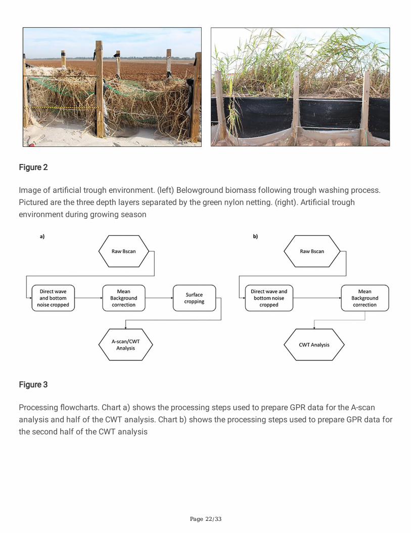
pictured, referred herein as a ‘trough’, was divided into 8 plots whose boundaries are de�ned by the postsmaking up the wall.  Plots were of a variable size, but were on average of length of 2.6 m, width 2.1 m,and depth 1.1 m. Prior to �lling the troughs with the sand, nylon nets were installed at three differentdepths. The nets were used during harvest to separate belowground biomass into different depth zonesfollowing a rinsing process. Photographs of the trough setup is shown in Figure 2. Plants were irrigatedvia a drip tape, and fertigated as needed via liquid fertilizer injector.

Fig 1 Plots and depth levels in the trough environment. From left to right, plots are numbered 1 – 8 (seetop view). The space labeled ‘B’ was designated as a blank area and no associated mass was harvested.The different depth zones are demarcated with different shades of gray

Fig 2 Image of arti�cial trough environment. (left) Belowground biomass following trough washingprocess. Pictured are the three depth layers separated by the green nylon netting. (right). Arti�cial troughenvironment during growing season

2.2 Field Data collection

In October 2017, the aboveground planted PSH09TX1 material was mowed to the soil media surface andthe troughs scanned with a prototype air-launched GPR antenna array developed by IDS Georadar(Golden, Colorado). The latter utilizes a unique air-launched resistively loaded-vee dipole antenna designwhich had been developed as a means to detect buried objects without the necessity of groundcontact (Kim and Scott 2005)(Nuzzo et al. 2014)(Montoya and Smith 1996). The antenna array unit hasbeen used in other published research (Dobreva et al. 2021)(Shen et al. 2019).

After the GPR scanning, the weed cloth barrier supporting the sides of the berm (shown in Figure 2, right)was removed exposing the bare sand matrix. The troughs were washed with a high-pressure water hoseover the course of one week resulting in the gradual exposure of root material (see Figure 2, left). The�brous root systems and rhizomes were captured by the nylon nets in the three different accessible depthzones. Measured from the soil surface, the thicknesses of each of the depth zones were 15, 45, and 45cm (see side view in Figure 1). The �brous roots and rhizomes were then harvested by hand. Plant crownswere included in the collected tissue of the top zone. Roots were severed where they crossed a nylon netsthat separating adjacent depth zones. Roots were collected within each plot (see Figure 1, top) at each ofthe three depth zones. Harvesting took place immediately after the washing process had concluded, andthe root material was dried in a greenhouse in order to preserve labile mass against microbialdegradation. The root samples were then re-washed in large plastic containers to remove excess sand.Samples were then hand-separated into two main tissue sub-groups: rhizomatous and �brous rootbiomass. Each sample was then dried in an oven at 60°C until its weight stabilized to remove variabilityin measured mass due to water content.

2.3 GPR processing

Page 7/33

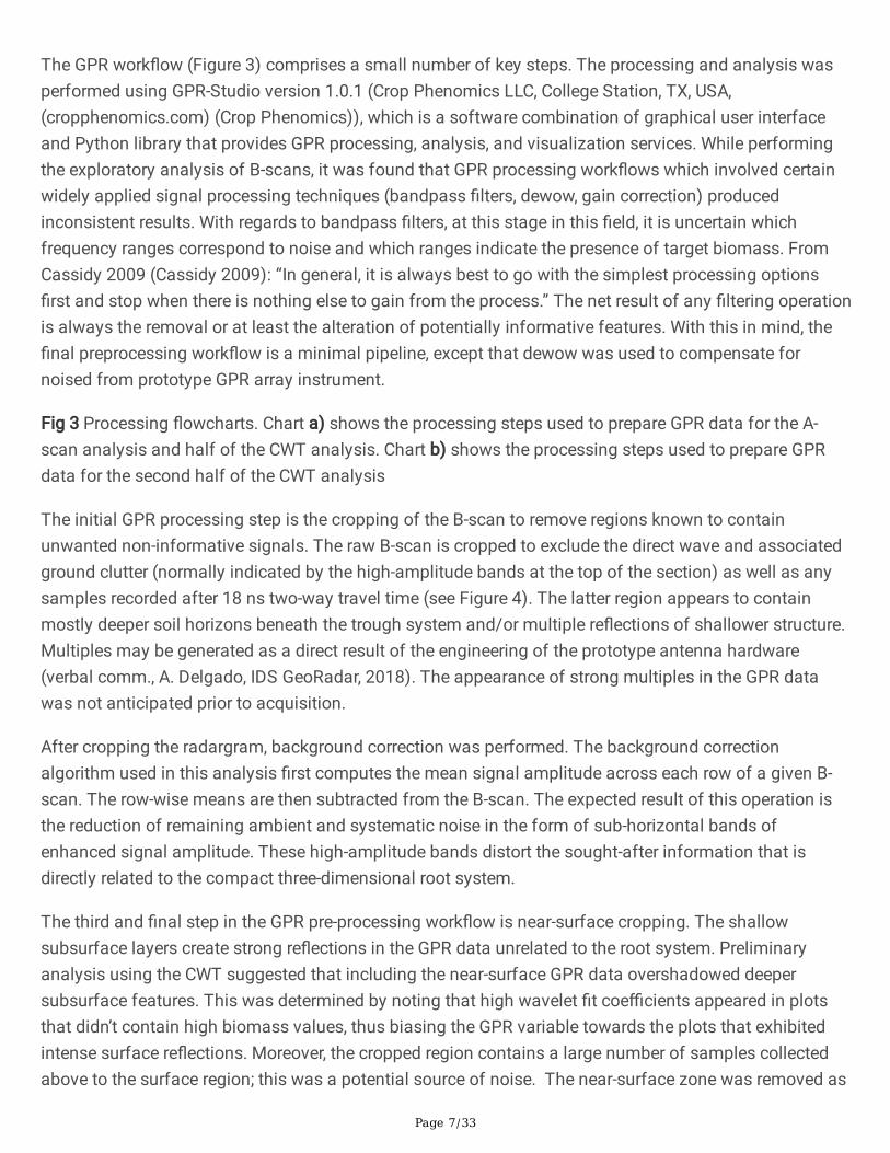
The GPR work�ow (Figure 3) comprises a small number of key steps. The processing and analysis wasperformed using GPR-Studio version 1.0.1 (Crop Phenomics LLC, College Station, TX, USA,(cropphenomics.com) (Crop Phenomics)), which is a software combination of graphical user interfaceand Python library that provides GPR processing, analysis, and visualization services. While performingthe exploratory analysis of B-scans, it was found that GPR processing work�ows which involved certainwidely applied signal processing techniques (bandpass �lters, dewow, gain correction) producedinconsistent results. With regards to bandpass �lters, at this stage in this �eld, it is uncertain whichfrequency ranges correspond to noise and which ranges indicate the presence of target biomass. FromCassidy 2009 (Cassidy 2009): “In general, it is always best to go with the simplest processing options�rst and stop when there is nothing else to gain from the process.” The net result of any �ltering operationis always the removal or at least the alteration of potentially informative features. With this in mind, the�nal preprocessing work�ow is a minimal pipeline, except that dewow was used to compensate fornoised from prototype GPR array instrument.

Fig 3 Processing �owcharts. Chart a) shows the processing steps used to prepare GPR data for the A-scan analysis and half of the CWT analysis. Chart b) shows the processing steps used to prepare GPRdata for the second half of the CWT analysis

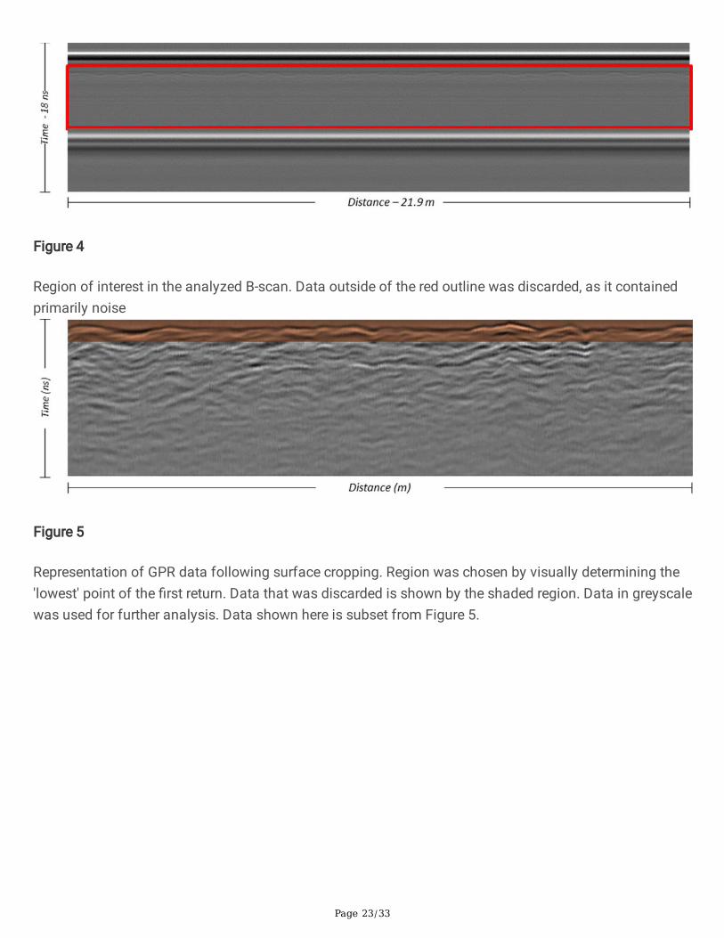
The initial GPR processing step is the cropping of the B-scan to remove regions known to containunwanted non-informative signals. The raw B-scan is cropped to exclude the direct wave and associatedground clutter (normally indicated by the high-amplitude bands at the top of the section) as well as anysamples recorded after 18 ns two-way travel time (see Figure 4). The latter region appears to containmostly deeper soil horizons beneath the trough system and/or multiple re�ections of shallower structure.Multiples may be generated as a direct result of the engineering of the prototype antenna hardware(verbal comm., A. Delgado, IDS GeoRadar, 2018). The appearance of strong multiples in the GPR datawas not anticipated prior to acquisition. 

After cropping the radargram, background correction was performed. The background correctionalgorithm used in this analysis �rst computes the mean signal amplitude across each row of a given B-scan. The row-wise means are then subtracted from the B-scan. The expected result of this operation isthe reduction of remaining ambient and systematic noise in the form of sub-horizontal bands ofenhanced signal amplitude. These high-amplitude bands distort the sought-after information that isdirectly related to the compact three-dimensional root system. 

The third and �nal step in the GPR pre-processing work�ow is near-surface cropping. The shallowsubsurface layers create strong re�ections in the GPR data unrelated to the root system. Preliminaryanalysis using the CWT suggested that including the near-surface GPR data overshadowed deepersubsurface features. This was determined by noting that high wavelet �t coe�cients appeared in plotsthat didn’t contain high biomass values, thus biasing the GPR variable towards the plots that exhibitedintense surface re�ections. Moreover, the cropped region contains a large number of samples collectedabove to the surface region; this was a potential source of noise.  The near-surface zone was removed as

Page 8/33

the overwhelming majority of plant biomass was harvested from the area below this zone as is shown inAppendix A, however analysis was simultaneously performed the same B-scans in which this surfaceregion was retained. Results in the analysis section are reported for both methodologies. A representativesurface-cropped section is shown in Figure 5.

Fig 4 Region of interest in the analyzed B-scan. Data outside of the red outline was discarded, as itcontained primarily noise

Fig 5 Representation of GPR data following surface cropping. Region was chosen by visually determiningthe 'lowest' point of the �rst return. Data that was discarded is shown by the shaded region. Data ingreyscale was used for further analysis. Data shown here is subset from Figure 5.

2.4 GPR analyses 

Following the GPR pre-processing, several analysis methods were used to interpret the processedradargrams. Steps were performed in both the time domain as well as the combined time/frequencydomain. The general objective of the analyses is to identify key diagnostic features from the radargramsthat correlate to the harvested subsurface biomass. 

2.4.1 Time domain signal analysis

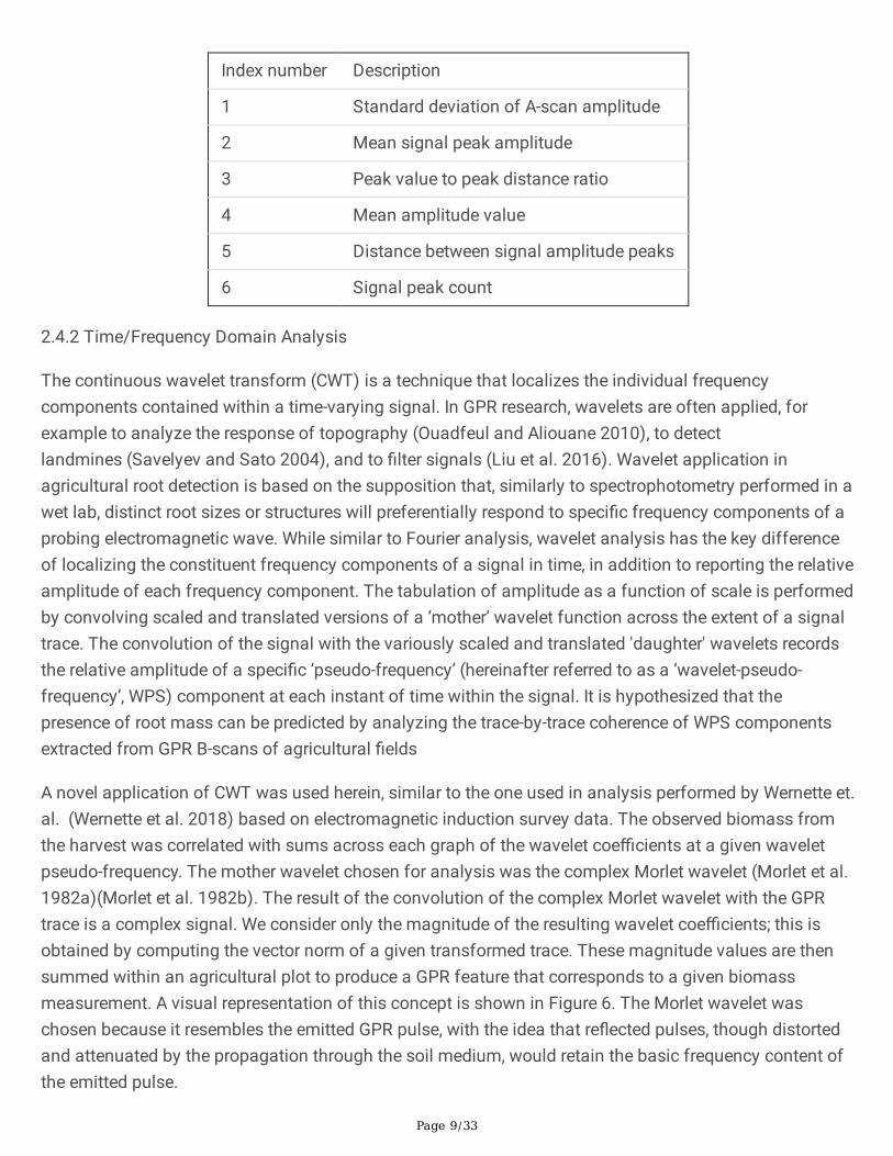
In the present study, the behavior of amplitude peaks is used as an indicator of variability within an A-scan signal. The working hypothesis is that one or more of a small panel of candidate amplitude-peakfeatures (see Table 1) are related to mass of belowground material; the use of A-scan features has someprecedent in life-science applications of GPR (Barton and Montagu 2004).

Each A-scan was analyzed by either extracting simple summary statistics (such as the mean andstandard deviation of the time-varying signal), or by extracting certain information regarding the peakamplitude values. The extracted quantities were then interpreted as candidate features related to the rootbiomass that was present in the trough at the time of scanning. Speci�cally, the A-scan features that wereextracted included the standard deviation of signal amplitude, the average (mean) signal peak value, theratio of peak value to the average time interval between peaks, the average amplitude value, the averagetime interval between peaks, and the number of peaks. This last feature was calculated after the A-scanwas truncated as per Figure 3. The foregoing analysis resulted in a set of feature values for each plot.The spatial variability of these features was also explored to understand how each metric varied withinan individual plot. While some of the spatial distributions appeared to be normal, others were skewed.Based on this observation, the feature distributions were characterized based on the median as ameasure of central tendency, as the median is relatively insensitive to outliers. The median was thuscalculated for each plot, and the resulting set of median feature values was correlated with harvestedbiomass measures. 

Table 1 Root density indices key

Page 9/33

Index number Description

1 Standard deviation of A-scan amplitude

2 Mean signal peak amplitude

3 Peak value to peak distance ratio     

4 Mean amplitude value 

5 Distance between signal amplitude peaks

6 Signal peak count

2.4.2 Time/Frequency Domain Analysis

The continuous wavelet transform (CWT) is a technique that localizes the individual frequencycomponents contained within a time-varying signal. In GPR research, wavelets are often applied, forexample to analyze the response of topography (Ouadfeul and Aliouane 2010), to detectlandmines (Savelyev and Sato 2004), and to �lter signals (Liu et al. 2016). Wavelet application inagricultural root detection is based on the supposition that, similarly to spectrophotometry performed in awet lab, distinct root sizes or structures will preferentially respond to speci�c frequency components of aprobing electromagnetic wave. While similar to Fourier analysis, wavelet analysis has the key differenceof localizing the constituent frequency components of a signal in time, in addition to reporting the relativeamplitude of each frequency component. The tabulation of amplitude as a function of scale is performedby convolving scaled and translated versions of a ‘mother’ wavelet function across the extent of a signaltrace. The convolution of the signal with the variously scaled and translated 'daughter' wavelets recordsthe relative amplitude of a speci�c ‘pseudo-frequency’ (hereinafter referred to as a ‘wavelet-pseudo-frequency’, WPS) component at each instant of time within the signal. It is hypothesized that thepresence of root mass can be predicted by analyzing the trace-by-trace coherence of WPS componentsextracted from GPR B-scans of agricultural �elds

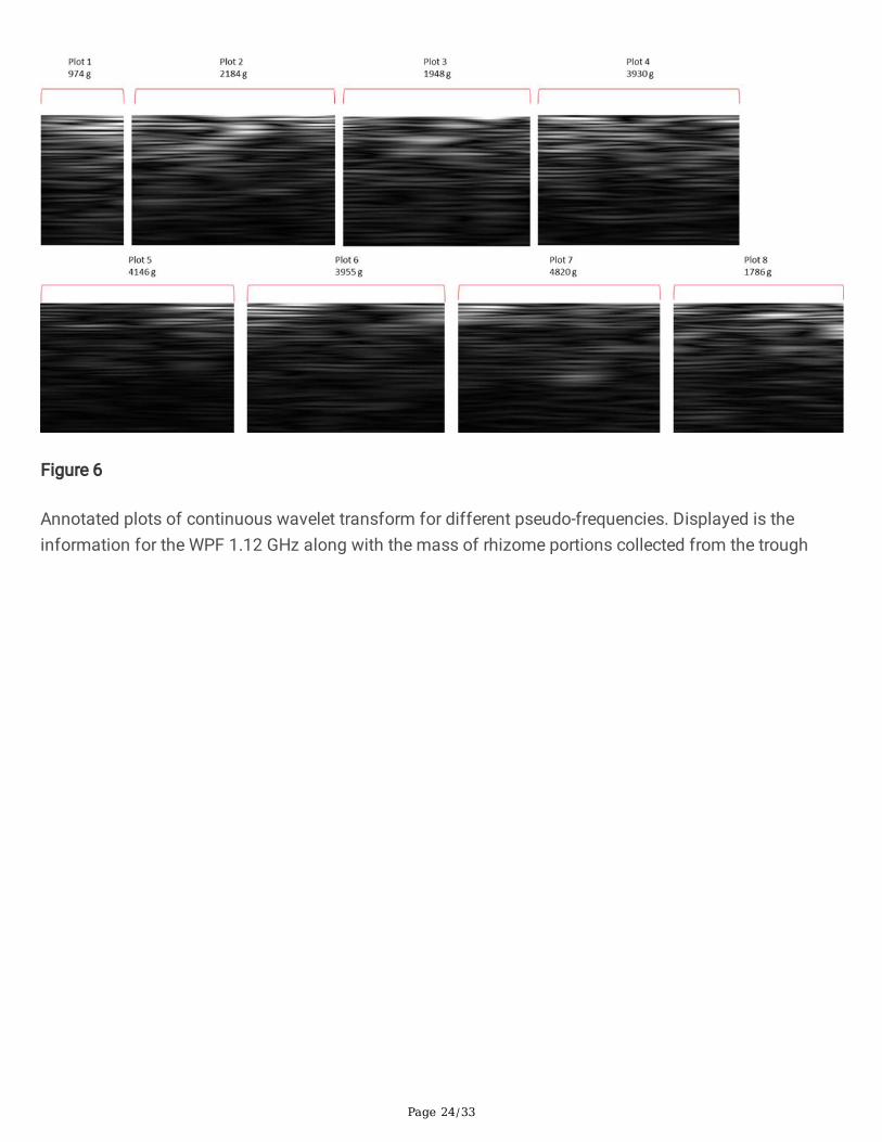
A novel application of CWT was used herein, similar to the one used in analysis performed by Wernette et.al.  (Wernette et al. 2018) based on electromagnetic induction survey data. The observed biomass fromthe harvest was correlated with sums across each graph of the wavelet coe�cients at a given waveletpseudo-frequency. The mother wavelet chosen for analysis was the complex Morlet wavelet (Morlet et al.1982a)(Morlet et al. 1982b). The result of the convolution of the complex Morlet wavelet with the GPRtrace is a complex signal. We consider only the magnitude of the resulting wavelet coe�cients; this isobtained by computing the vector norm of a given transformed trace. These magnitude values are thensummed within an agricultural plot to produce a GPR feature that corresponds to a given biomassmeasurement. A visual representation of this concept is shown in Figure 6. The Morlet wavelet waschosen because it resembles the emitted GPR pulse, with the idea that re�ected pulses, though distortedand attenuated by the propagation through the soil medium, would retain the basic frequency content ofthe emitted pulse. 

Page 10/33

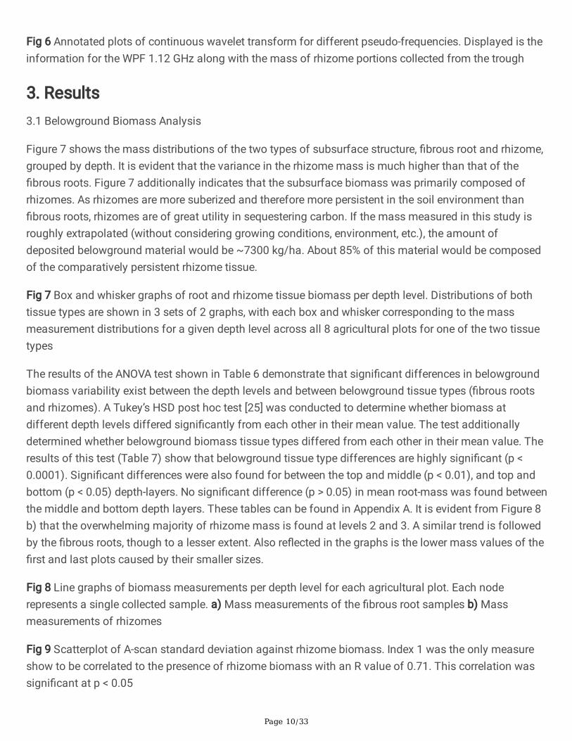
Fig 6 Annotated plots of continuous wavelet transform for different pseudo-frequencies. Displayed is theinformation for the WPF 1.12 GHz along with the mass of rhizome portions collected from the trough

3. Results3.1 Belowground Biomass Analysis

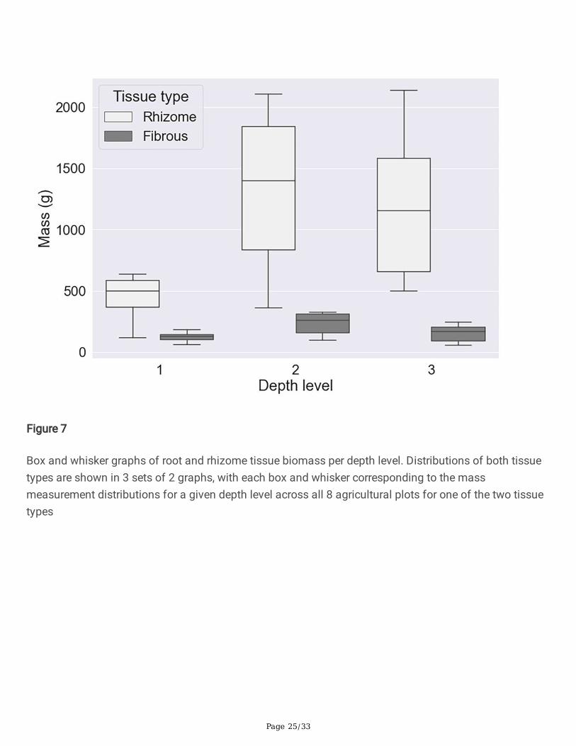
Figure 7 shows the mass distributions of the two types of subsurface structure, �brous root and rhizome,grouped by depth. It is evident that the variance in the rhizome mass is much higher than that of the�brous roots. Figure 7 additionally indicates that the subsurface biomass was primarily composed ofrhizomes. As rhizomes are more suberized and therefore more persistent in the soil environment than�brous roots, rhizomes are of great utility in sequestering carbon. If the mass measured in this study isroughly extrapolated (without considering growing conditions, environment, etc.), the amount ofdeposited belowground material would be ~7300 kg/ha. About 85% of this material would be composedof the comparatively persistent rhizome tissue.

Fig 7 Box and whisker graphs of root and rhizome tissue biomass per depth level. Distributions of bothtissue types are shown in 3 sets of 2 graphs, with each box and whisker corresponding to the massmeasurement distributions for a given depth level across all 8 agricultural plots for one of the two tissuetypes

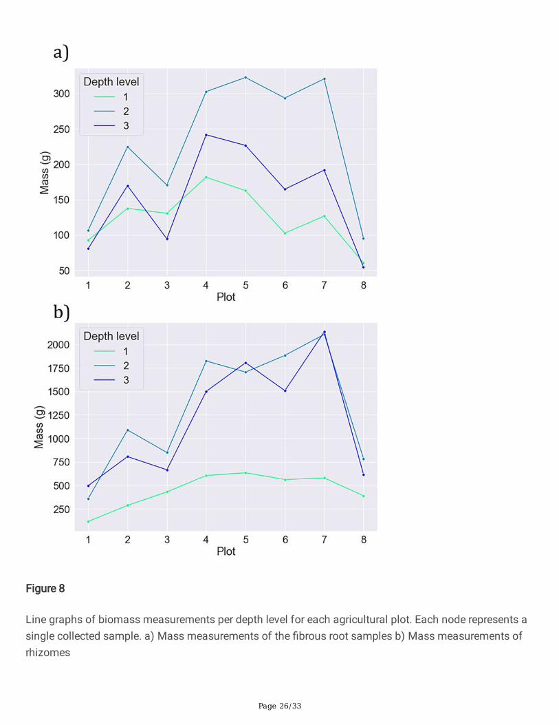
The results of the ANOVA test shown in Table 6 demonstrate that signi�cant differences in belowgroundbiomass variability exist between the depth levels and between belowground tissue types (�brous rootsand rhizomes). A Tukey’s HSD post hoc test [25] was conducted to determine whether biomass atdifferent depth levels differed signi�cantly from each other in their mean value. The test additionallydetermined whether belowground biomass tissue types differed from each other in their mean value. Theresults of this test (Table 7) show that belowground tissue type differences are highly signi�cant (p <0.0001). Signi�cant differences were also found for between the top and middle (p < 0.01), and top andbottom (p < 0.05) depth-layers. No signi�cant difference (p > 0.05) in mean root-mass was found betweenthe middle and bottom depth layers. These tables can be found in Appendix A. It is evident from Figure 8b) that the overwhelming majority of rhizome mass is found at levels 2 and 3. A similar trend is followedby the �brous roots, though to a lesser extent. Also re�ected in the graphs is the lower mass values of the�rst and last plots caused by their smaller sizes.

Fig 8 Line graphs of biomass measurements per depth level for each agricultural plot. Each noderepresents a single collected sample. a) Mass measurements of the �brous root samples b) Massmeasurements of rhizomes 

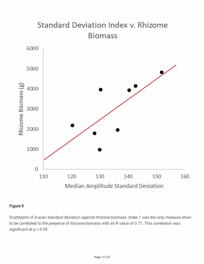
Fig 9 Scatterplot of A-scan standard deviation against rhizome biomass. Index 1 was the only measureshow to be correlated to the presence of rhizome biomass with an R value of 0.71. This correlation wassigni�cant at p < 0.05

Page 11/33

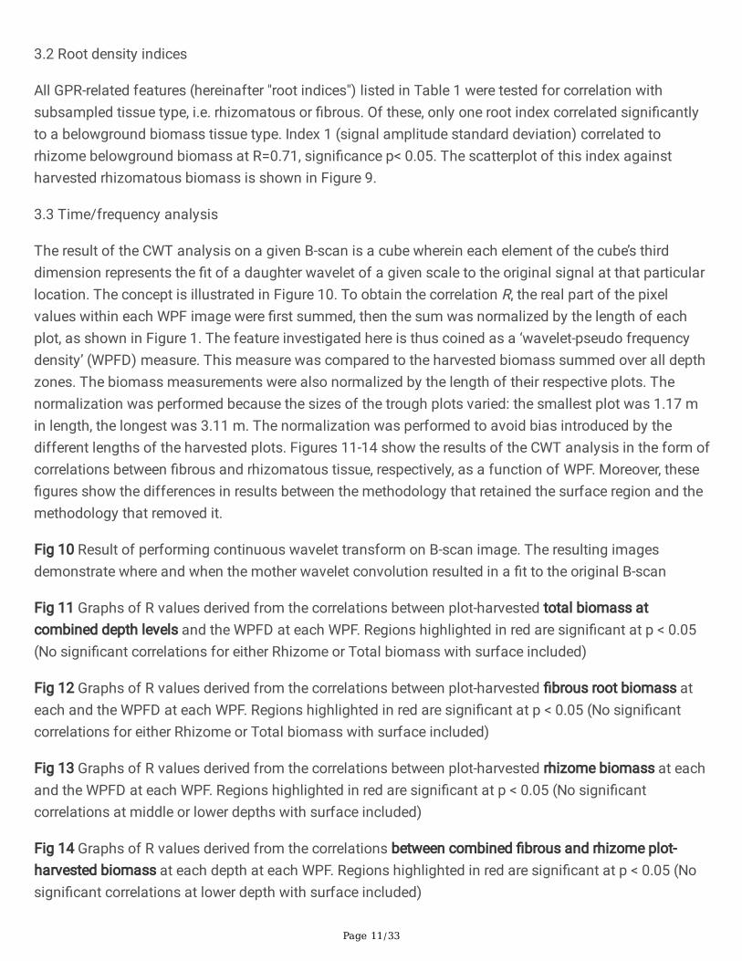
3.2 Root density indices

All GPR-related features (hereinafter "root indices") listed in Table 1 were tested for correlation withsubsampled tissue type, i.e. rhizomatous or �brous. Of these, only one root index correlated signi�cantlyto a belowground biomass tissue type. Index 1 (signal amplitude standard deviation) correlated torhizome belowground biomass at R=0.71, signi�cance p< 0.05. The scatterplot of this index againstharvested rhizomatous biomass is shown in Figure 9.

3.3 Time/frequency analysis

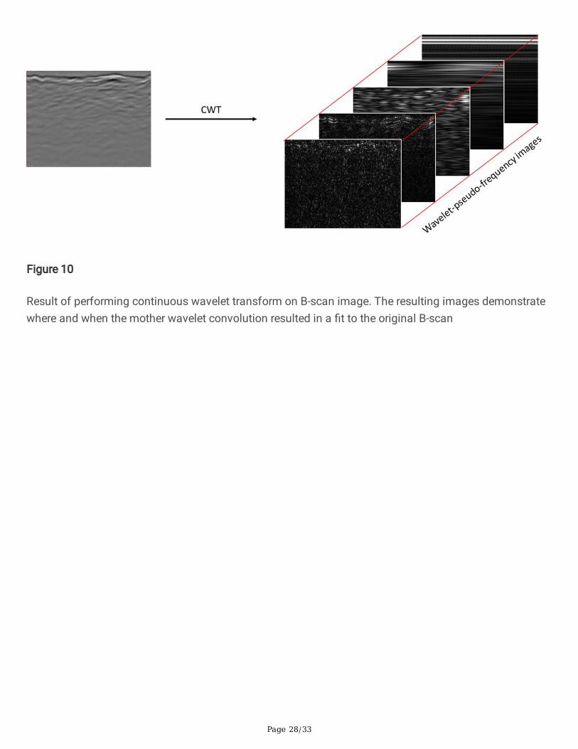
The result of the CWT analysis on a given B-scan is a cube wherein each element of the cube’s thirddimension represents the �t of a daughter wavelet of a given scale to the original signal at that particularlocation. The concept is illustrated in Figure 10. To obtain the correlation R, the real part of the pixelvalues within each WPF image were �rst summed, then the sum was normalized by the length of eachplot, as shown in Figure 1. The feature investigated here is thus coined as a ‘wavelet-pseudo frequencydensity’ (WPFD) measure. This measure was compared to the harvested biomass summed over all depthzones. The biomass measurements were also normalized by the length of their respective plots. Thenormalization was performed because the sizes of the trough plots varied: the smallest plot was 1.17 min length, the longest was 3.11 m. The normalization was performed to avoid bias introduced by thedifferent lengths of the harvested plots. Figures 11-14 show the results of the CWT analysis in the form ofcorrelations between �brous and rhizomatous tissue, respectively, as a function of WPF. Moreover, these�gures show the differences in results between the methodology that retained the surface region and themethodology that removed it.

Fig 10 Result of performing continuous wavelet transform on B-scan image. The resulting imagesdemonstrate where and when the mother wavelet convolution resulted in a �t to the original B-scan

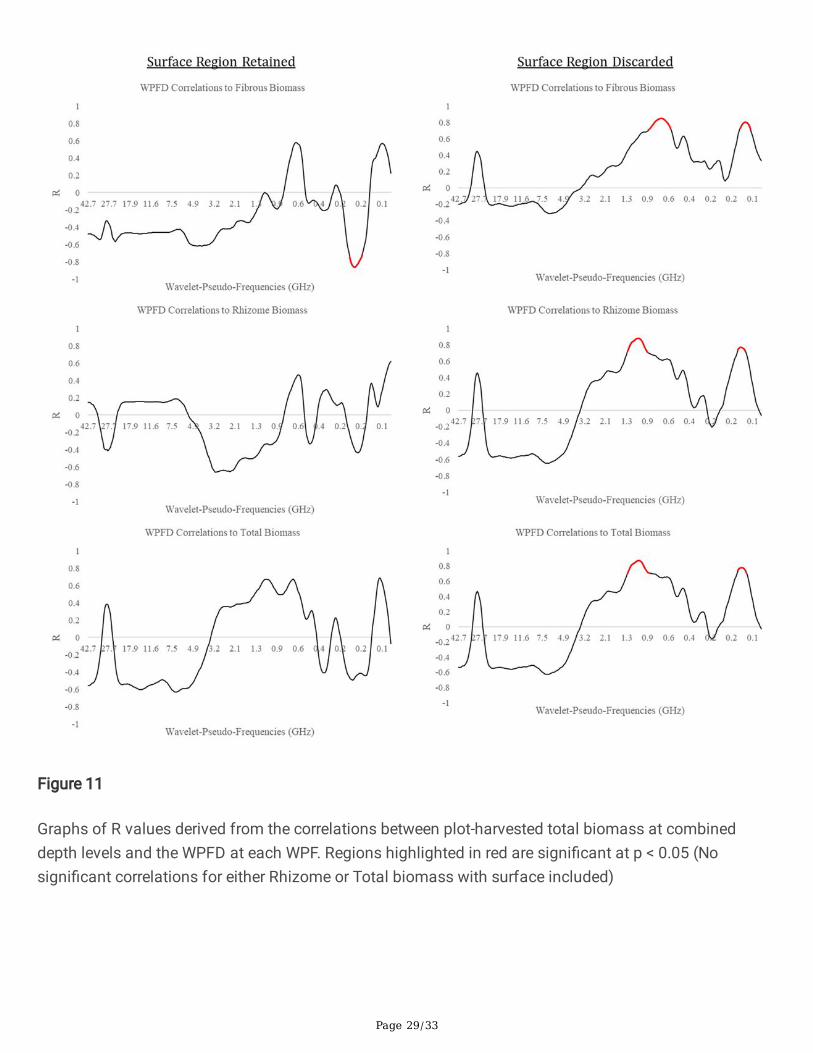
Fig 11 Graphs of R values derived from the correlations between plot-harvested total biomass atcombined depth levels and the WPFD at each WPF. Regions highlighted in red are signi�cant at p < 0.05(No signi�cant correlations for either Rhizome or Total biomass with surface included)

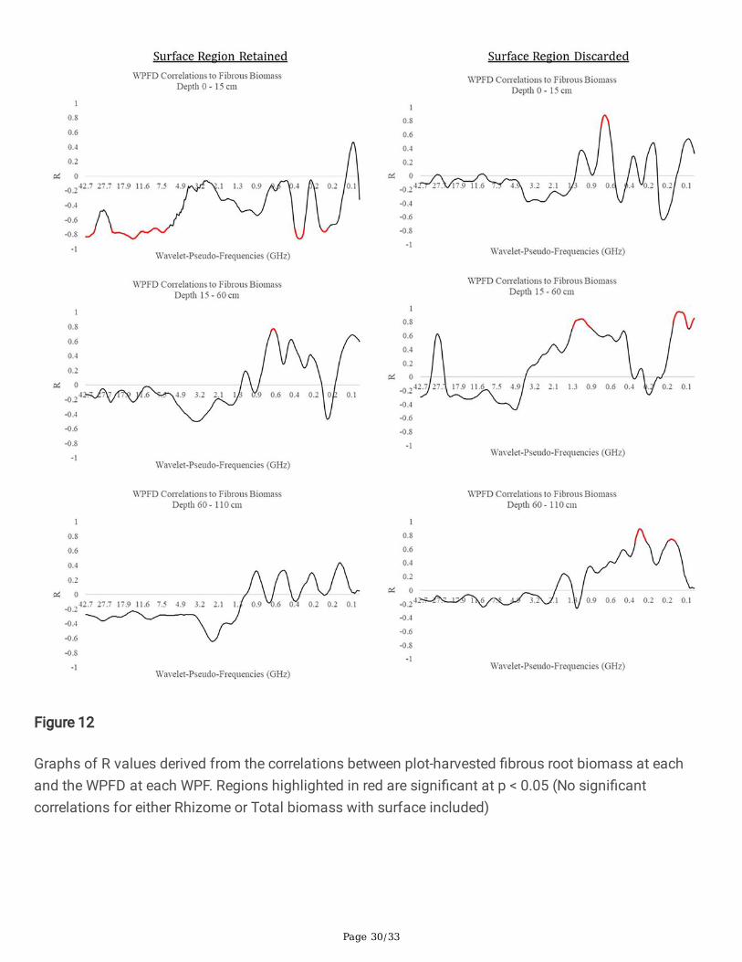
Fig 12 Graphs of R values derived from the correlations between plot-harvested �brous root biomass ateach and the WPFD at each WPF. Regions highlighted in red are signi�cant at p < 0.05 (No signi�cantcorrelations for either Rhizome or Total biomass with surface included)

Fig 13 Graphs of R values derived from the correlations between plot-harvested rhizome biomass at eachand the WPFD at each WPF. Regions highlighted in red are signi�cant at p < 0.05 (No signi�cantcorrelations at middle or lower depths with surface included)

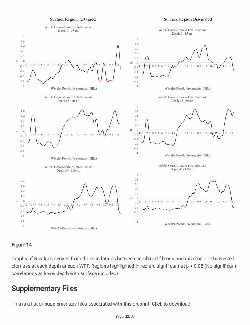
Fig 14 Graphs of R values derived from the correlations between combined �brous and rhizome plot-harvested biomass at each depth at each WPF. Regions highlighted in red are signi�cant at p < 0.05 (Nosigni�cant correlations at lower depth with surface included)

Page 12/33

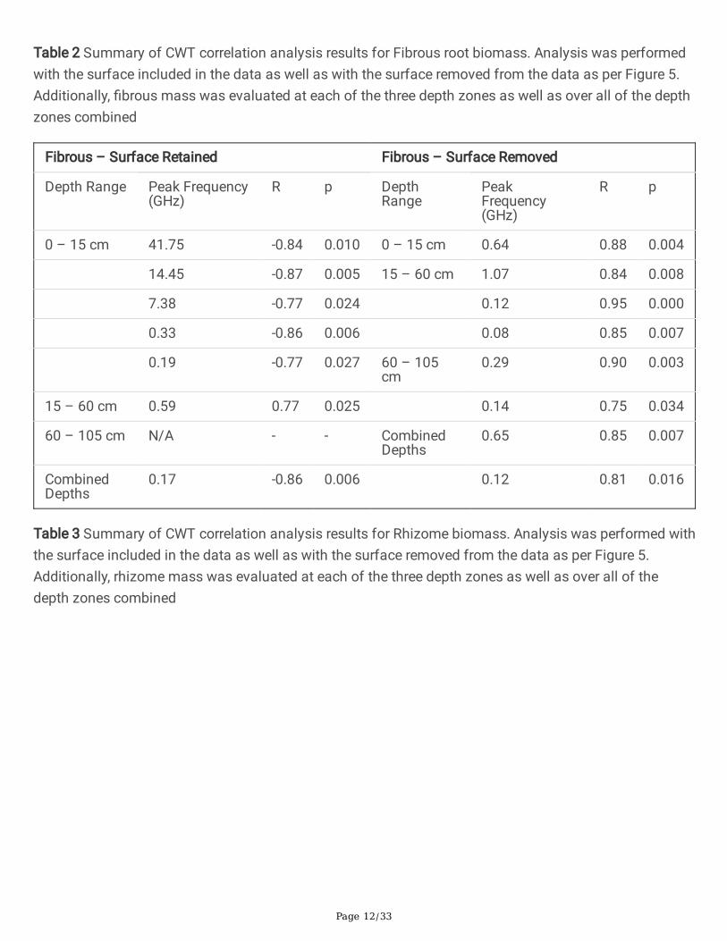
Table 2 Summary of CWT correlation analysis results for Fibrous root biomass. Analysis was performedwith the surface included in the data as well as with the surface removed from the data as per Figure 5.Additionally, �brous mass was evaluated at each of the three depth zones as well as over all of the depthzones combined

Fibrous – Surface Retained Fibrous – Surface Removed

Depth Range Peak Frequency(GHz)

R p DepthRange

PeakFrequency(GHz)

R p

0 – 15 cm 41.75 -0.84 0.010 0 – 15 cm 0.64 0.88 0.004

14.45 -0.87 0.005 15 – 60 cm 1.07 0.84 0.008

7.38 -0.77 0.024 0.12 0.95 0.000

0.33 -0.86 0.006 0.08 0.85 0.007

0.19 -0.77 0.027 60 – 105cm

0.29 0.90 0.003

15 – 60 cm 0.59 0.77 0.025 0.14 0.75 0.034

60 – 105 cm N/A - - CombinedDepths

0.65 0.85 0.007

CombinedDepths

0.17 -0.86 0.006 0.12 0.81 0.016

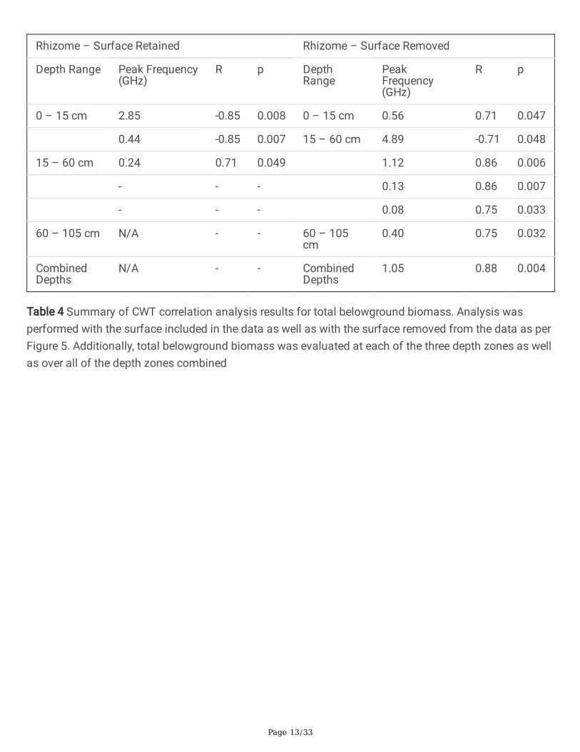
Table 3 Summary of CWT correlation analysis results for Rhizome biomass. Analysis was performed withthe surface included in the data as well as with the surface removed from the data as per Figure 5.Additionally, rhizome mass was evaluated at each of the three depth zones as well as over all of thedepth zones combined

Page 13/33

Rhizome – Surface Retained Rhizome – Surface Removed

Depth Range Peak Frequency(GHz)

R p DepthRange

PeakFrequency(GHz)

R p

0 – 15 cm 2.85 -0.85 0.008 0 – 15 cm 0.56 0.71 0.047

0.44 -0.85 0.007 15 – 60 cm 4.89 -0.71 0.048

15 – 60 cm 0.24 0.71 0.049 1.12 0.86 0.006

- - - 0.13 0.86 0.007

- - - 0.08 0.75 0.033

60 – 105 cm N/A - - 60 – 105cm

0.40 0.75 0.032

CombinedDepths

N/A - - CombinedDepths

1.05 0.88 0.004

Table 4 Summary of CWT correlation analysis results for total belowground biomass. Analysis wasperformed with the surface included in the data as well as with the surface removed from the data as perFigure 5. Additionally, total belowground biomass was evaluated at each of the three depth zones as wellas over all of the depth zones combined

Page 14/33

Fibrous – Surface Retained Fibrous – Surface Removed

Depth Range Peak Frequency(GHz)

R p DepthRange

PeakFrequency(GHz)

R p

0 – 15 cm 42.67 -0.82 0.013 0 – 15 cm 0.57 0.75 0.034

14.45 -0.90 0.002 - - -

7.54 -0.71 0.047 - - -

0.31 -0.83 0.010 - - -

0.19 -0.82 0.013 - - -

0.14 -0.80 0.018 - - -

15 – 60 cm 1.05 0.86 0.006 15 – 60 cm 1.12 0.87 0.005

0.57 0.77 0.027 0.12 0.88 0.004

0.12 0.82 0.013 0.08 0.76 0.027

60 – 105 cm 0.86 0.71 0.050 60 – 105cm

0.40 0.75 0.031

- - - 0.31 0.75 0.033

CombinedDepths

N/A - - CombinedDepths

1.03 0.87 0.004

- - - 0.13 0.78 0.022

The inclusion or exclusion of the near-surface portion of the radargrams affected the WPF’s at whichcorrelations peaked. A summary of all of speci�c peak information for each root type and depth is givenin Table 2, Table 3, and Table 4 for �brous roots, rhizomes, and total mass respectively. Notably, theinclusion of the near-surface region resulted in strong negative correlations between WPFD and massdensity at the 0 – 15 cm depth zone and a smaller number of signi�cantly correlated WPF’s at the 15 –60 cm and 60 – 110 cm depth zones. Conversely, the removal of the near-surface region resulted in morestrong positive relationships between WPFD and mass density across all depth zones. This is shown inFigures 11 – 14 as the wider red bands of indicated signi�cance (p < 0.05). Little consistency was foundbetween depth zones in terms of signi�cant WPF for each root type. Interestingly, when the near-surfaceregion is removed, all root types correlate signi�cantly to similar WPF ranges. This trend can be seen onthe right halves of Figures 11 – 14. Generally, 0 – 15 cm peaked at ~0.6 GHz, 15 – 60 cm peaked at ~1.4GHz, and 60 – 110 cm peaked at ~0.4 GHz.

4. Discussion

Page 15/33

Root detection by GPR shows promise for further development both in theory, since roots present adielectric contrast to the host soil, and based on previous studies documented in the literature (Bartonand Montagu 2004)(Delgado et al. 2017)(Dobreva et al. 2021). The present study assesses the feasibilityof root biomass quanti�cation by exploring correlations between features extracted from GPR responsesand harvested belowground biomass. A similar A-scan level approach has been previously demonstrated (Barton and Montagu 2004) in which signal features related to tree roots were analyzed. Other studieshave adopted an image analysis approach to quantify the presence of belowground biomass. Forexample, Delgado et. al (Delgado et al. 2017) performed radargram pixel counts to quantify the mass ofcassava tubers. Dobreva et al. (Dobreva et al. 2021) performed a similar pixel level image analysis topredict peanut yield. While image-analysis approaches should be further investigated for the �brous rootsystems of grasses, the lack of a single large, discrete target object characteristic of large roots motivatesthe current study toward trace-based and time/frequency-based analysis. 

Root structures in this study were binary classi�ed as �brous or rhizomatous, a helpful distinction toexplore detectability with ground penetrating radar. The possibility exists of detecting an individualrhizome, although the λ/4 limit (Everett 2013) at 0.9-2.7 GHz prevents resolution of objects less than~0.88 cm in length. The resolution limit is much larger than a typical diameter of �ne roots or root hairs,but potentially of the same scale as rhizomes and the spatial changes in root architecture and/or the rootsystem’s zone of in�uence (i.e. the area within which water interacts with the root system). The relativelylarge size of the entire root system and its zone of in�uence is a positive indicator for detectability andbelowground mass quanti�cation. However, spatially variable soil moisture affects the interactionbetween the GPR signal and the root system; an increase in soil water content will reduce the dielectriccontrast, and hence re�ectivity, of the root and the surrounding soil. Somewhat paradoxically, thereduction in dielectric contrast may assist the detection of smaller roots near the soil surface. The higherdielectric constant of saturated soil slows the signal velocity such that acquired GPR data exhibits higherspatial resolution. This tradeoff is discussed in Liu et al’s paper  (Liu et al. 2018) on GPR detection ofwheat roots. 

A-scan analysis involves the extraction of features from individual GPR traces. A-scan-level featureextraction methods have previously been used to study the subsurface in non-agricultural settings. Herewe describe a few examples. Variation in signal amplitude, for example, was used to characterize acoastal depositional environment (Leandro et al. 2019). Reversal of trace polarity is often indicative ofsubsurface voids, which aids discovery of buried caskets (Conyers 2015). The �rst derivative of thesignal, instantaneous frequency, and similarity between successive traces are GPR A-scan-level featuresthat were used to characterize sedimentary structures in sand dunes (Zhao et al. 2018). Differences in thetwo-way-travel time of the '�rst return' was used as a feature to understand how soil moisture affects theGPR ground wave (Galagedara et al. 2003). Peaks in A-scan amplitude have been used to extract theclassic 'hyperbolae'   B-scan level features in GPR (Li and Zhou 2007). 

The time-domain analysis of individual signal traces yielded only one GPR feature, or index, with asigni�cant correlation to belowground biomass. As different indices were tested against the two different

Page 16/33

root-tissue types, most combinations revealed no signi�cant relationship to the harvested biomass. Thetotal mass and the rhizome mass are very similar, such that these secondary structures of the sorghumhybrid are responsible for a large fraction of the deposited belowground biomass. The dominance ofrhizome biomass over �brous root biomass suggests that time-domain correlations with GPR indices forrhizome biomass and total belowground biomass should be similar. However, while the rhizome biomasscorrelated signi�cantly to the standard deviation of signal amplitude, the total root biomass did notsigni�cantly relate to any of the tested indices. Since rhizomes are an important subsurface structurewith high carbon sequestration capacity, the positive correlation result is encouraging, however theinsigni�cant correlation with total belowground biomass contradicts the positive result. 

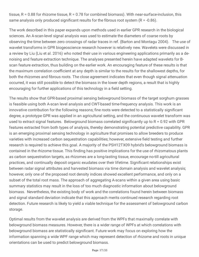
The wavelet analysis produced high correlations at several distinct WPFs, depending on the depth level,tissue type of the biomass under test, and the inclusion or exclusion of the near-surface region of theradargrams. Most interestingly, the correlation switched from strongly negative with surface inclusion tostrongly positive with surface exclusion. Moreover, with the surface inclusion analysis, the relationshipsat the 15 – 60 cm depth zones switched back to being strongly positive. Negative relationships betweenroot biomass and GPR signal features have been reported in previous literature (Liu et al. 2018), andcorrelations have been shown to switch from negative to positive at progressive depths (Dobreva et al.2021), however their signi�cance is still not well understood. A possible explanation for negativerelationships is that the presence of a root zone may result in less soil compaction and thus cause aweaker re�ection at the surface, but this would need to be experimentally con�rmed. As the frequency ofa GPR signal return corresponding to a large object would typically be low, the expectation is thatbelowground tissue with a larger radius would be correlated with lower wavelet frequency. In general thiswas true for the dataset with the surface included, however surface exclusion resulted in a pattern ofrhizome tissue showing correlation peaks at higher WPFs than the �brous root system. This wasunexpected, as rhizomes are much larger in diameter than individual roots in the �brous system. Apossible explanation, warranting further study, is that individual �brous roots do not re�ect EM radiationin the frequency range of the current antenna, but are rather detected as an ‘aggregate root zone’. Thishypothesis is partially supported by the results shown in Figure 11 as both �brous roots and rhizomescorrelate highly with similar WPF ranges. There is little consistency with which WPFs correlate stronglywith biomass as burial depth increases. The lack of a clear relationship between WPF and biomass ateach burial depth suggests that morphological structures may respond differently at varying burialdepths. The lack of a consistent radar signature could present a signi�cant challenge moving forward, asthe eventual goal for this technology is its application in realistic agricultural settings where soilconditions and root mass are not known beforehand. There does appear to be a relationship between theWPF at which high correlations occur and the size of the root structures that are detected. This is shownby the results of the near-surface-exclusion analysis on the right sides of Figure 11, Figure 12, Figure 13,and Figure 14. However, this relationship also requires con�rmation, as it is not clearly understood atpresent. Interestingly, the methodology that correlated belowground biomass to the near-surface-excludedGPR signal without regard to biomass depth performed well on both tissue types (R = 0.81 for �brous root

Page 17/33

tissue, R = 0.88 for rhizome tissue, R = 0.78 for combined biomass). With near-surface-inclusion, thissame analysis only produced signi�cant results for the �brous root system (R = -0.86).

The work described in this paper expands upon methods used in earlier GPR research in the biologicalsciences. An A-scan-level signal analysis was used to estimate the diameters of coarse roots byobserving the time between zero crossings of radar traces in ref. (Barton and Montagu 2004).   The use ofwavelet transforms in GPR biogeoscience research however is relatively new. Wavelets were discussed ina review by Liu (Liu et al. 2016) who noted their use in various engineering applications primarily as a de-noising and feature extraction technique. The analyses presented herein have adapted wavelets for B-scan feature extraction, thus building on the earlier work. An encouraging feature of these results is thatthe maximum correlation coe�cient at any depth is similar to the results for the shallowest depths, forboth the rhizomes and �brous roots. The close agreement indicates that even though signal attenuationoccurred, it was still possible to detect the biomass in the lower depth regions, a result that is highlyencouraging for further applications of this technology in a �eld setting. 

The results show that GPR-based proximal sensing belowground biomass of the target sorghum grassesis feasible using both A-scan level analysis and CWT-based time-frequency analysis. This work is aninnovative contribution for the following reasons; �ne roots were detected to a statistically signi�cantdegree, a prototype GPR was applied in an agricultural setting, and the continuous wavelet transform wasused to extract signal features.  Belowground biomass correlated signi�cantly up to R = 0.92 with GPRfeatures extracted from both types of analysis, thereby demonstrating potential predictive capability. GPRis an emerging proximal sensing technology in agriculture that promises to allow breeders to producevarieties with increased carbon sequestration capabilities; however, extensive �eld testing and furtherresearch is required to achieve this goal. A majority of the PSH12TX09 hybrid’s belowground biomass iscontained in the rhizome tissue. This �nding has positive implications for the use of rhizomatous plantsas carbon sequestration targets, as rhizomes are a long-lasting tissue, encourage no-till agriculturalpractices, and continually deposit organic exudates over their lifetime. Signi�cant relationships existbetween radar signal attributes and harvested biomass via time domain analysis and wavelet analysis;however, only one of the proposed root density indices showed excellent performance, and only on asubset of the total root mass. The approach of aggregating A-scans within a given area using basicsummary statistics may result in the loss of too much diagnostic information about belowgroundbiomass.  Nevertheless, the existing body of work and the correlations found herein between biomassand signal standard deviation indicate that this approach merits continued research regarding rootdetection. Future research is likely to yield a viable technique for the assessment of belowground carbonstorage.

Optimal results from the wavelet analysis are derived from the WPFs that maximally correlate withbelowground biomass measures. However, there is a wider range of WPFs at which correlations withbelowground biomass are statistically signi�cant. Future work may focus on exploring how theinformation spanning a wide WPF range which may represent detection of rhizome and roots in uniqueorientations can be used to predict belowground biomass.

Page 18/33

AbbreviationsWavelet Pseudo-Frequency (WPF)

Wavelet Pseudo-Frequency Density (WPFD)

Ground Penetrating Radar (GPR)

Continuous Wavelet Transform (CWT)

Plot – Agricultural plot

DeclarationsAcknowledgements

This work was supported with grants from the National Science Foundation award number 1543957—BREAD PHENO: High Throughput Phenotyping Early Stage Root Bulking in Cassava using GroundPenetrating Radar to Dirk B. Hays, and by the Department of Energy of the United States (ARPA-E Award,No. DE-AR0000662)—Development of ground penetrating radar for enhanced root phenotyping andcarbon sequestration also to Dirk B. Hays.

ReferencesAllen, M.R., O.P. Dube, W. Solecki, F. Aragón-Durand, W. Cramer, S. Humphreys, M. Kainuma, J. Kala, N.Mahowald, Y. Mulugetta, R. Perez, M. Wairiu  and KZ (2018) Global Warming of 1.5°C. An IPCC SpecialReport on the impacts of global warming of 1.5°C above pre-industrial levels and related globalgreenhouse gas emission pathways, in the context of strengthening the global response to the threat ofclimate change,

Barton CVM, Montagu KD (2004) Detection of tree roots and determination of root diameters by groundpenetrating radar under optimal conditions. Tree Physiol 24:1323–1331.https://doi.org/10.1093/treephys/24.12.1323

Butnor JR, Doolittle JA, Johnsen KH, et al (2003) Utility of Ground-Penetrating Radar as a Root BiomassSurvey Tool in Forest Systems. Soil Sci Soc Am J 67:1607. https://doi.org/10.2136/sssaj2003.1607

Butnor JR, Doolittle JA, Kress L, et al (2001) Use of ground-penetrating radar to study tree roots in thesoutheastern United States. Tree Physiol 21:1269–1278. https://doi.org/11696414

Cassidy N (2009) Ground penetrating radar data processing, modelling and analysis, First Edit. Elsevier

Conyers LB (2015) Analysis and interpretation of GPR datasets for integrated archaeological mapping.Near Surf Geophys 13:645–651. https://doi.org/10.3997/1873-0604.2015018

Crop Phenomics L GPR Studio

Page 19/33

Delgado A, Hays DB, Bruton RK, et al (2017) Ground penetrating radar: A case study for estimating rootbulking rate in cassava (Manihot esculenta Crantz). Plant Methods 13:. https://doi.org/10.1186/s13007-017-0216-0

Dobreva ID, Ruiz-Guzman HA, Barrios-Perez I, et al (2021) Thresholding Analysis and Feature Extractionfrom 3D Ground Penetrating Radar Data for Noninvasive Assessment of Peanut Yield. Remote Sens13:1896. https://doi.org/10.3390/rs13101896

Everett M (2013) Near-surface Applied Geophysics

Galagedara LW, Parkin GW, Redman JD (2003) An analysis of the ground-penetrating radar direct groundwave method for soil water content measurement. Hydrol Process 17:3615–3628.https://doi.org/10.1002/hyp.1351

García-robledo C, Kuprewicz EK, Staines CL, et al (2016) Limited tolerance by insects to high temperaturesacross tropical elevational gradients and the implications of global warming for extinction. 113:.https://doi.org/10.1073/pnas.1507681113

Gebhart DL, Johnson HB, Mayeux HS, Polleym HW (1994) The CRP increases oil organic carbon. J soilwater Conserv 49:488–492

Jessup RW, Klein RR, Burson BL, et al (2017)  Registration of Perennial Sorghum bicolor × S. propinquumLine PSH12TX09 . J Plant Regist 11:76–79. https://doi.org/10.3198/jpr2015.09.0054crgs

Kerry JT, Álvarez-noriega M, Álvarez-romero JG, et al (2017) Global warming and recurrent massbleaching of corals. https://doi.org/10.1038/nature21707

Kim K, Scott WR (2005) Design of resistively loaded vee dipole for ultrawide-band ground-penetratingradar applications. IEEE Trans Antennas Propag 53:2525–2532.https://doi.org/10.1109/TAP.2005.852292

Lane HM, Murray SC (2021) High Throughput can produce better decisions than high accuracy whenphenotyping plant populations. Crop Sci. https://doi.org/10.1002/csc2.20514

Leandro CG, Barboza EG, Caron F, de Jesus FAN (2019) GPR trace analysis for coastal depositionalenvironments of southern Brazil. J Appl Geophys 162:1–12.https://doi.org/10.1016/j.jappgeo.2019.01.002

Ledo A, Smith P, Zerihun A, et al (2020) Changes in soil organic carbon under perennial crops. Glob ChangBiol 26:4158–4168. https://doi.org/10.1111/gcb.15120

Lemus R, Lal R (2005) Bioenergy crops and carbon sequestration. CRC Crit Rev Plant Sci 24:1–21.https://doi.org/10.1080/07352680590910393

Page 20/33

Li TJ, Zhou ZO (2007) Fast extraction of hyperbolic signatures in GPR. 2007 Int Conf Microw Millim WaveTechnol ICMMT ’07 3–5. https://doi.org/10.1109/ICMMT.2007.381489

Liu X, Dong X, Leskovar DI, et al (2018) Ground penetrating radar (GPR) detects �ne roots of agriculturalcrops in the �eld. Plant Soil 517–531

Liu X, Dong X, Leskovar DI (2016) Ground penetrating radar for underground sensing in agriculture: Areview. Int Agrophysics 30:533–543. https://doi.org/10.1515/intag-2016-0010

Montoya TP, Smith GS (1996) Resistivity-loaded Vee antennas for short-pulse ground penetrating radar.IEEE Antennas Propag Soc AP-S Int Symp 3:2068–2071. https://doi.org/10.1109/aps.1996.550015

Morlet J, Arens G, Fourgeau E, Giard D (1982a) Wave propagation and sampling theory - Part I. Complexsignal and scattering in multilayered media. Geophysics 47:203–221. https://doi.org/10.1190/1.1441328

Morlet J, Arens G, Fourgeau E, Giard D (1982b) Wave propagation and sampling theory - Part II. Samplingtheory and complex waves. Geophysics 47:222–236. https://doi.org/10.1190/1.1441329

Nuzzo L, Alli G, Guidi R, et al (2014) A new densely-sampled Ground Penetrating Radar array for landminedetection. In: Proceedings of the 15th International Conference on Ground Penetrating Radar. IEEE, pp969–974

Ouadfeul SA, Aliouane L (2010) Multiscale analysis of 3D GPR data using thecontinuous WaveletTransform. Proc 13th Internarional Conf Gr Penetrating Radar, GPR 2010 1–4.https://doi.org/10.1109/ICGPR.2010.5550177

Paez-Garcia A, Motes CM, Scheible WR, et al (2015) Root traits and phenotyping strategies for plantimprovement. Plants 4:334–355. https://doi.org/10.3390/plants4020334

Resource N, Collins F (2001) GRASSLAND MANAGEMENT AND CONVERSION INTO GRASSLAND :EFFECTS ON SOIL CARBON. 11:343–355

Savelyev TG, Sato M (2004) Comparative analysis of UWB deconvolution and feature-extractionalgorithms for GPR landmine detection. Detect Remediat Technol Mines Minelike Targets IX 5415:1008.https://doi.org/10.1117/12.541748

Schmidt GA, Ruedy RA, Miller RL, Lacis AA (2010) Attribution of the present-day total greenhouse effect. JGeophys Res Atmos 115:1–6. https://doi.org/10.1029/2010JD014287

Shen X, Foster T, Baldi H, et al (2019) Quanti�cation of soil organic carbon in biochar-amended soil usingground penetrating radar (GPR). Remote Sens 11:1–12. https://doi.org/10.3390/rs11232874

Thomas H, Thomas HM, Ougham H (2000) Annuality, perenniality and cell death. J Exp Bot 51:1781–1788. https://doi.org/10.1093/jexbot/51.352.1781

Page 21/33

Utsi E (2017) Ground Penetrating Radar: theory and practice

Wernette P, Houser C, Weymer BA, et al (2018) In�uence of a spatially complex framework geology onbarrier island geomorphology. Mar Geol 398:151–162. https://doi.org/10.1016/j.margeo.2018.01.011

Xiong S, Thomas K (2010) Carbon-allocation dynamics in reed canary grass as affected by soil type andfertilization rates in northern Sweden. Acta Agric Scand Sect B Soil Plant Sci 60:24–32.https://doi.org/10.1080/09064710802558518

Zhao W, Forte E, Fontolan G, Pipan M (2018) Advanced GPR imaging of sedimentary features: Integratedattribute analysis applied to sand dunes. Geophys J Int 213:147–156.https://doi.org/10.1093/gji/ggx541

(2016) Attribution of extreme weather events in the context of climate change. National Academies Press

Figures

Figure 1

Plots and depth levels in the trough environment. From left to right, plots are numbered 1 – 8 (see topview). The space labeled ‘B’ was designated as a blank area and no associated mass was harvested. Thedifferent depth zones are demarcated with different shades of gray

Page 22/33

Figure 2

Image of arti�cial trough environment. (left) Belowground biomass following trough washing process.Pictured are the three depth layers separated by the green nylon netting. (right). Arti�cial troughenvironment during growing season

Figure 3

Processing �owcharts. Chart a) shows the processing steps used to prepare GPR data for the A-scananalysis and half of the CWT analysis. Chart b) shows the processing steps used to prepare GPR data forthe second half of the CWT analysis

Page 23/33

Figure 4

Region of interest in the analyzed B-scan. Data outside of the red outline was discarded, as it containedprimarily noise

Figure 5

Representation of GPR data following surface cropping. Region was chosen by visually determining the'lowest' point of the �rst return. Data that was discarded is shown by the shaded region. Data in greyscalewas used for further analysis. Data shown here is subset from Figure 5.

Page 24/33

Figure 6

Annotated plots of continuous wavelet transform for different pseudo-frequencies. Displayed is theinformation for the WPF 1.12 GHz along with the mass of rhizome portions collected from the trough

Page 25/33

Figure 7

Box and whisker graphs of root and rhizome tissue biomass per depth level. Distributions of both tissuetypes are shown in 3 sets of 2 graphs, with each box and whisker corresponding to the massmeasurement distributions for a given depth level across all 8 agricultural plots for one of the two tissuetypes

Page 26/33

Figure 8

Line graphs of biomass measurements per depth level for each agricultural plot. Each node represents asingle collected sample. a) Mass measurements of the �brous root samples b) Mass measurements ofrhizomes

Page 27/33

Figure 9

Scatterplot of A-scan standard deviation against rhizome biomass. Index 1 was the only measure showto be correlated to the presence of rhizome biomass with an R value of 0.71. This correlation wassigni�cant at p < 0.05

Page 28/33

Figure 10

Result of performing continuous wavelet transform on B-scan image. The resulting images demonstratewhere and when the mother wavelet convolution resulted in a �t to the original B-scan

Page 29/33

Figure 11

Graphs of R values derived from the correlations between plot-harvested total biomass at combineddepth levels and the WPFD at each WPF. Regions highlighted in red are signi�cant at p < 0.05 (Nosigni�cant correlations for either Rhizome or Total biomass with surface included)

Page 30/33

Figure 12

Graphs of R values derived from the correlations between plot-harvested �brous root biomass at eachand the WPFD at each WPF. Regions highlighted in red are signi�cant at p < 0.05 (No signi�cantcorrelations for either Rhizome or Total biomass with surface included)

Page 31/33

Figure 13

Graphs of R values derived from the correlations between plot-harvested rhizome biomass at each andthe WPFD at each WPF. Regions highlighted in red are signi�cant at p < 0.05 (No signi�cant correlationsat middle or lower depths with surface included)

Page 32/33

Figure 14

Graphs of R values derived from the correlations between combined �brous and rhizome plot-harvestedbiomass at each depth at each WPF. Regions highlighted in red are signi�cant at p < 0.05 (No signi�cantcorrelations at lower depth with surface included)

Supplementary Files

This is a list of supplementary �les associated with this preprint. Click to download.

Page 33/33

AppendixA.docx