ph.d. thesis thermo-hydro-mechanical impacts of carbon...
TRANSCRIPT
Ph.D. Thesis
Thermo-Hydro-Mechanical Impacts of Carbon Dioxide (CO2) Injection in Deep Saline Aquifers.
by
Víctor Vilarrasa Riaño
Hydrogeology Group (GHS)
Department of Geotechnical Engineering and Geosciences, Technical University of Catalonia (UPC-BarcelonaTech)
Institute of Environmental Assessment and Water Research (IDAEA), Spanish Research Council (CSIC)
Supervised by:
Jesús Carrera
Sebastià Olivella
June, 2012

This thesis was funded by the Spanish Ministry of Science and Innovation (MCI), through the
“Formación de Profesorado Universitario” Program, and the “Colegio de Ingenieros de
Caminos, Canales y Puertos – Catalunya”; and was developed in the framework of two projects:
the ALM/09/18 project of the Spanish Ministry of Industry, Energy and Tourism through the
CIUDEN foundation (www.ciuden.es) and the “MUSTANG” project (from the European
Community’s Seventh Framework Programme FP7/2007-2013 under grant agreement nº
227286; www.co2mustang.eu).

To my pillar

i
I. Abstract
Coupled thermo-hydro-mechanical effects related to geologic carbon storage should be
understood and quantified in order to demonstrate to the public that carbon dioxide
(CO2) injection is safe. This Thesis aims to improve such understanding by developing
methods to: (1) evaluate the CO2 plume geometry and fluid pressure evolution; (2)
define a field test to characterize the maximum sustainable injection pressure and the
hydromechanical properties of the aquifer and the caprock; and (3) propose an energy
efficient injection concept that improves the caprock mechanical stability in most
geological settings due to thermo-mechanical effects.
First, we investigate numerically and analytically the effect of CO2 density and viscosity
variability on the position of the interface between the CO2-rich phase and the
formation brine. We introduce a correction to account for CO2 compressibility (density
variations) and viscosity variations in current analytical solutions. We find that the error
in the interface position caused by neglecting CO2 compressibility is relatively small
when viscous forces dominate. However, it can become significant when gravity forces
dominate, which is likely to occur at late times and/or far from the injection well.
Second, we develop a semianalytical solution for the CO2 plume geometry and fluid
pressure evolution, accounting for CO2 compressibility and buoyancy effects in the
injection well. We formulate the problem in terms of a CO2 potential that facilitates
solution in horizontal layers, in which we discretize the aquifer. We find that when a
prescribed CO2 mass flow rate is injected, CO2 advances initially through the top
portion of the aquifer. As CO2 pressure builds up, CO2 advances not only laterally, but
also vertically downwards. However, the CO2 plume does not necessarily occupy the
whole thickness of the aquifer. Both CO2 plume position and fluid pressure compare
well with numerical simulations. Therefore, this solution facilitates quick evaluations of
the CO2 plume position and fluid pressure distribution when injecting supercritical CO2
in a deep saline aquifer.
Third, we study potential failure mechanisms, which could lead to CO2 leakage, in an
axysimmetric horizontal aquifer-caprock system, using a viscoplastic approach.

ii
Simulations illustrate that, depending on boundary conditions, the least favorable
situation may occur at the beginning of injection. However, in the presence of low-
permeability boundaries, fluid pressure continues to rise in the whole aquifer, which
may compromise the caprock integrity in the long-term.
Next, we propose a hydromechanical characterization test to estimate the
hydromechanical properties of the aquifer and caprock at the field scale. We obtain
curves for overpressure and vertical displacement as a function of the volumetric strain
term obtained from a dimensional analysis of the hydromechanical equations. We can
then estimate the values of the Young’s modulus and the Poisson ratio of the aquifer
and the caprock by introducing field measurements in these plots. The results indicate
that induced microseismicity is more likely to occur in the aquifer than in the caprock.
The onset of microseismicity in the caprock can be used to define the maximum
sustainable injection pressure to ensure a safe permanent CO2 storage.
Finally, we analyze the thermodynamic evolution of CO2 and the thermo-hydro-
mechanical response of the formation and the caprock to liquid (cold) CO2 injection.
We find that injecting CO2 in liquid state is energetically more efficient than in
supercritical state because liquid CO2 is denser than supercritical CO2. Therefore, the
pressure required at the wellhead for a given CO2 pressure in the aquifer is much lower
for liquid than for gas or supercritical injection. In fact, the overpressure required at the
aquifer is also smaller because a smaller fluid volume is displaced. The temperature
decrease close to the injection well induces a stress reduction due to thermal
contraction of the media. This can lead to shear slip of pre-existing fractures in the
aquifer for large temperature contrasts in stiff rocks, which could enhance injectivity. In
contrast, the mechanical stability of the caprock is improved in stress regimes where
the maximum principal stress is the vertical.

iii
II. Resumen
Los procesos termo-hidro-mecánicos relacionados con el almacenamiento geológico
de carbono deben ser entendidos y cuantificados para demostrar a la opinión pública
de que la inyección de dióxido de carbono (CO2) es segura. Esta Tesis tiene como
objetivo mejorar dicho conocimiento mediante el desarrollo de métodos para: (1)
evaluar la evolución tanto de la geometría de la pluma de CO2 como de la presión de
los fluidos; (2) definir un ensayo de campo que permita caracterizar la presión de
inyección máxima sostenible y los parámetros hidromecánicos de las rocas sello y
almacén; y (3) proponer un nuevo concepto de inyección que es energéticamente
eficiente y que mejora la estabilidad de la roca sello en la mayoría de escenarios
geológicos debido a efectos termo-mecánicos.
Primero, investigamos numérica y analíticamente los efectos de la variabilidad de la
densidad y viscosidad del CO2 en la posición de la interfaz entre la fase rica en CO2 y
la salmuera de la formación. Introducimos una corrección para tener en cuenta dicha
variabilidad en las soluciones analíticas actuales. Encontramos que el error producido
en la posición de la interfaz al despreciar la compresibilidad del CO2 es relativamente
pequeño cuando dominan las fuerzas viscosas. Sin embargo, puede ser significativo
cuando dominan las fuerzas de gravedad, lo que ocurre para tiempos y/o distancias
largas de inyección.
Segundo, desarrollamos una solución semianalítica para la evolución de la geometría
de la pluma de CO2 y la presión de fluido, teniendo en cuenta tanto la compresibilidad
del CO2 como los efectos de flotación dentro del pozo. Formulamos el problema en
términos de un potencial de CO2 que facilita la solución en capas horizontales, en las
que hemos discretizado el acuífero. El CO2 avanza inicialmente por la porción superior
del acuífero. Pero a medida que aumenta la presión de CO2, la pluma crece no solo
lateralmente, sino también hacia abajo, aunque no tiene porqué llegar a ocupar todo el
espesor del acuífero. Tanto la interfaz CO2-salmuera como la presión de fluido
muestran una buena comparación con las simulaciones numéricas.
En tercer lugar, estudiamos posibles mecanismos de rotura, que podrían llegar a
producir fugas de CO2, en un sistema acuífero-sello con simetría radial, utilizando un

iv
modelo viscoplástico. Las simulaciones ilustran que, dependiendo de las condiciones
de contorno, el momento más desfavorable ocurre al inicio de la inyección. Sin
embargo, si los contornos son poco permeables, la presión de fluido continúa
aumentando en todo el acuífero, lo que podría llegar a comprometer la estabilidad de
la roca sello a largo plazo.
Para evaluar dichos problemas, proponemos un ensayo de caracterización
hidromecánica a escala de campo para estimar las propiedades hidromecánicas de las
rocas sello y almacén. Obtenemos curvas para la sobrepresión y el desplazamiento
vertical en función del término de la deformación volumétrica obtenido del análisis
adimensional de las ecuaciones hidromecánicas. Ajustando las medidas de campo a
estas curvas se pueden estimar los valores del módulo de Young y el coeficiente de
Poisson del acuífero y del sello. Los resultados indican que la microsismicidad
inducida tiene más probabilidades de ocurrir en el acuífero que en el sello. El inicio de
la microsismicidad en el sello marca la presión de inyección máxima sostenible para
asegurar un almacenamiento permanente de CO2 seguro.
Finalmente, analizamos la evolución termodinámica del CO2 y la respuesta termo-
hidro-mecánica de las rocas sello y almacén a la inyección de CO2 líquido (frío).
Encontramos que inyectar CO2 en estado líquido es energéticamente más eficiente
porque al ser más denso que el CO2 supercrítico, requiere menor presión en cabeza
de pozo para una presión dad en el acuífero. De hecho, esta presión también es
menor en el almacén porque se desplaza un volumen menor de fluido. La disminución
de temperatura en el entorno del pozo induce una reducción de tensiones debido a la
contracción térmica del medio. Esto puede producir deslizamiento de fracturas
existentes en acuíferos formados por rocas rígidas bajo contrastes de temperatura
grandes, lo que podría incrementar la inyectividad de la roca almacén. Por otro lado, la
estabilidad mecánica de la roca sello mejora cuando la tensión principal máxima es la
vertical.
v
III. Resum
Els processos termo-hidro-mecànics relacionats amb l’emmagatzematge geològic de
carboni han de ser entesos i quantificats per tal de demostrar a l’opinió pública de que
la injecció de diòxid de carboni (CO2) és segura. Aquesta Tesi té com a objectiu
millorar aquest coneixement mitjançant el desenvolupament de mètodes per a: (1)
avaluar l'evolució tant de la geometria del plomall de CO2 com de la pressió dels fluids;
(2) definir un assaig de camp que permeti caracteritzar la pressió d'injecció màxima
sostenible i els paràmetres hidromecànics de les roques segell i magatzem; i (3)
proposar un nou concepte d'injecció que és energèticament eficient i que millora
l'estabilitat de la roca segell en la majoria d’escenaris geològics a causa d'efectes
termo-mecànics.
Primer, investiguem numèricament i analítica els efectes de la variabilitat de la densitat
i viscositat del CO2 en la posició de la interfície entre la fase rica en CO2 i la salmorra
de la formació. Introduïm una correcció per tal de tenir en compte aquesta variabilitat
en les solucions analítiques actuals. Trobem que l'error produït en la posició de la
interfície en menysprear la compressibilitat del CO2 és relativament petit quan dominen
les forces viscoses. Malgrat això, l’error pot ser significatiu quan dominen les forces de
gravetat, la qual cosa té lloc per a temps i/o distàncies llargues d'injecció.
Segon, desenvolupem una solució semianalítica per a l'evolució de la geometria del
plomall de CO2 i la pressió de fluid, tenint en compte tant la compressibilitat del CO2
com els efectes de flotació dins del pou. Formulem el problema en termes d'un
potencial de CO2 que facilita la solució en capes horitzontals, en les quals hem
discretitzat l'aqüífer. El CO2 avança inicialment per la porció superior de l'aqüífer. Però
a mesura que augmenta la pressió de CO2, el plomall de CO2 no només creix
lateralment, sinó que també ho fa cap avall, encara que no té perquè arribar a ocupar
tot el gruix de l'aqüífer. Tant la interfície CO2-salmorra com la pressió de fluid mostren
una bona comparació amb les simulacions numèriques.
En tercer lloc, estudiem possibles mecanismes de trencament, que podrien arribar a
produir fugues de CO2, en un sistema aqüífer-segell amb simetria radial, utilitzant un
model viscoplàstic. Les simulacions il·lustren que, depenent de les condicions de

vi
contorn, el moment més desfavorable té lloc a l'inici de la injecció. Tot i això, si els
contorns són poc permeables, la pressió de fluid continua augmentant en tot l'aqüífer,
la qual cosa podria arribar a comprometre l'estabilitat de la roca segell a llarg termini.
Per a avaluar aquests problemes, proposem un assaig de caracterització
hidromecànica a escala de camp per a estimar les propietats hidromecàniques de les
roques segell i magatzem. Obtenim corbes per a la sobrepressió i el desplaçament
vertical en funció del terme de la deformació volumètrica obtingut de l'anàlisi
adimensional de les equacions hidromecàniques. Ajustant les mesures de camp a
aquestes corbes es poden estimar els valors del mòdul de Young i el coeficient de
Poisson de l'aqüífer i del segell. Els resultats indiquen que la microsismicitat induïda té
més probabilitats d'ocórrer en l'aqüífer que en el segell. L'inici de la microsismicitat en
el segell marca la pressió d'injecció màxima sostenible per tal d’assegurar un
emmagatzematge permanent de CO2 segur.
Finalment, analitzem l'evolució termodinàmica del CO2 i la resposta termo-hidro-
mecànica de les roques segell i magatzem a la injecció de CO2 líquid (fred). Trobem
que injectar CO2 en estat líquid és energèticament més eficient perquè al ser més dens
que el CO2 supercrític, requereix una pressió menor al cap de pou per a una pressió
donada a l’aqüífer. De fet, aquesta pressió també és menor a l’aqüífer perquè es
desplaça un volum menor de fluid. La disminució de temperatura a l'entorn del pou
indueix una reducció de tensions a causa de la contracció tèrmica del medi. Això pot
produir lliscament de fractures existents en aqüífers formats per roques rígides sota
contrastos de temperatura grans, la qual cosa podria incrementar la injectivitat de la
roca magatzem. D’altra banda, l'estabilitat mecànica de la roca segell millora quan la
tensió principal màxima és la vertical.

vii
IV. Acknowledgements
Many people have left a footprint in my work and myself during my PhD studies, each
in their own special way. I would like to express my most sincere gratitude to all of
them.
First of all, I would like to express my deepest gratitude to my supervisors Jesús
Carrera and Sebastià Olivella for trusting me and letting me fly under their wise
guidance. It has been a privilege and a pleasure to work with them and to continuously
learn from them.
I greatly appreciate Orlando Silva for sharing his code of flow through pipes and for
revising the implementation of the CO2 thermal properties in CODE_BRIGHT.
I would also like to express my utmost gratitude to Prof. Hamdi Tchelepi for his
supervision and guidance during my stay at Stanford University. I would also like to
thank the people who made my stay there comfortable, especially to Maria Elenius,
Juan Argote, Joan Murcia, Anna Borrell and Jihoon Kim. I am also thankful to Dr. Jens
Birkholzer for giving me the opportunity to give a seminar at the Lawrence Berkeley
Nacional Laboratory. I am grateful to Prof. Sally Benson, Dr. Jonny Rutqvist and Dr.
Quanlin Zhou for fruitful discussion and their interest in my work.
I would like to express my most sincere gratitude to all the people with whom I have
worked with during these years. A special mention is deserved to those scientists with
whom I have the privilege to share the coauthorship of a publication: Diogo Bolster,
Marco Dentz, Orlando Silva, Estanislao Pujades, Anna Jurado, Francesca de Gaspari,
Silvia de Simone, Enric Vázquez-Suñé, Daniel Fernández-García, Xavier Sánchez-
Vila, Daniel Tartakovsky, Tomofumi Koyama, Lanru Jing and Ivars Neretnieks.
Needless to say, I am deeply grateful to all my fellow students from the Civil
Engineering School, but especially to my fellows of the Hydrogeology Group. I would
also like to thank the people who work to make our life easier at University: Teresa
García, Silvia Aranda, Ana Martínez. Thanks also to Jordi Cama’s joy, who does not
understand that love can coexist with the rivalry of Barça-Madrid supporters. I am

viii
especially thankful to Alberto Herrero, Estanis Pujades, Albert Nardi, Daniele Pedretti,
Joaquín Jiménez and Diogo Bolster for their friendship and sharing my worries.
I would like to thank the MUSTANG team, especially to Dr. Jacob Bear for his
perseverance in improving the work, Dr. Auli Niemi for coordinating the project and Dr.
Jacob Bensabat, Dr. Henry Power, Dr. Tore Torp for fruitful discussion.
I would also like to thank the CIUDEN team, especially to Dr. Andrés Pérez-Estaún, Dr.
Ramón Carbonell, Dr. José Luís Fuentes, Dr. Jordi Bruno, Dr. Oriol Montserrat from
whom I have learnt a lot. I am particularly grateful to Dr. Modesto Montoto for his
interest in my research and encouraging me to be enterprising.
I would like to extend my special thanks to the friends I made at the Civil Engineering
School of Barcelona: Oriol, Guillem, Jonatan, Pau, Núria, Marc, Quim, Ignasi, Edu,
Jordi, with whom I have shared uncountable laughs, but unfortunately some worries
lately because of the bad moments that our profession is undergoing these days.
I would like to express my special thanks to all my family, especially to my parents, who
have always given me support and smoothed the way.
Last but not least, my dearest thanks to Pilar for all the good moments we have lived
together and for her patience, understanding and unconditional support. Thanks for
encouraging me in taking the hard decision of starting my PhD studies.

ix
V. List of Contents
I. Abstract ................................................................................................................................ i
II. Resumen ............................................................................................................................ iii
III. Resum ................................................................................................................................. v
IV. Acknowledgements ..........................................................................................................vii
V. List of Contents ..................................................................................................................ix
1. Introduction ......................................................................................................................... 1
1.1. Background and objectives ....................................................................................... 1
1.2. Thesis layout ............................................................................................................... 7
2. Effects of CO2 Compressibility on CO2 Storage in Deep Saline Aquifers ................. 9
2.1. Introduction .................................................................................................................. 9
2.2. Multiphase flow. The role of compressibility ......................................................... 11
2.3. Analytical solutions ................................................................................................... 15
2.3.1. Abrupt interface approximation ...................................................................... 15
2.3.2. Nordbotten et al. (2005) approach ................................................................. 16
2.3.3. Dentz and Tartakovsky (2009a) approach ................................................... 17
2.4. Compressibility correction ....................................................................................... 18
2.5. Application ................................................................................................................. 21
2.5.1. Injection scenarios ............................................................................................ 21
2.5.2. Case 1: Viscous forces dominate ................................................................... 23
2.5.3. Case 2: Comparable gravity and viscous forces ......................................... 24
2.5.4. Case 3: Gravity forces dominate .................................................................... 27
2.6. Conclusions ............................................................................................................... 30
3. Semianalytical Solution for CO2 Plume Shape and Pressure Evolution during
CO2 Injection in Deep Saline Aquifers ...................................................................................... 33
3.1. Introduction ................................................................................................................ 33
x
3.2. Problem formulation ................................................................................................. 35
3.3. Semianalytical solution ............................................................................................ 37
3.3.1. Radial injection of compressible CO2 ............................................................ 37
3.3.2. Prescribed CO2 mass flow rate ...................................................................... 42
3.3.3. Prescribed CO2 pressure ................................................................................. 42
3.4. Algorithm .................................................................................................................... 43
3.5. Application ................................................................................................................. 44
3.5.1. Spreadsheet programming .............................................................................. 44
3.5.2. Model setup ....................................................................................................... 45
3.5.3. Validation of the semianalytical solution ....................................................... 46
3.5.4. CO2 plume thickness ........................................................................................ 50
3.6. Discussion and conclusions .................................................................................... 51
4. Coupled Hydromechanical Modeling of CO2 Sequestration in Deep Saline
Aquifers ......................................................................................................................................... 53
4.1. Introduction ................................................................................................................ 53
4.2. Methods ..................................................................................................................... 56
4.2.1. Geometry ........................................................................................................... 56
4.2.2. Fluid mechanics ................................................................................................ 56
4.2.3. Geomechanics .................................................................................................. 58
4.2.4. Numerical solution ............................................................................................ 61
4.3. Fluid pressure evolution .......................................................................................... 61
4.3.1. Infinitely acting aquifer ..................................................................................... 61
4.3.2. Radial aquifer with a low-permeability boundary ......................................... 62
4.4. Hydromechanical coupling ...................................................................................... 64
4.5. Discussion and conclusions .................................................................................... 70
5. Hydromechanical Characterization of CO2 Injection Sites ........................................ 75
5.1. Introduction ................................................................................................................ 75
xi
5.2. Mechanical properties of rocks ............................................................................... 77
5.3. Hydromechanical characterization test ................................................................. 79
5.3.1. Test description ................................................................................................. 79
5.3.2. Problem formulation ......................................................................................... 80
5.3.3. Numerical solution ............................................................................................ 87
5.4. Results ....................................................................................................................... 88
5.4.1. Hydromechanical behaviour ........................................................................... 88
5.4.2. Sensitivity analysis ........................................................................................... 91
5.4.3. Induced microseismicity analysis ................................................................... 97
5.5. Discussion ............................................................................................................... 103
5.6. Conclusion ............................................................................................................... 106
6. Liquid CO2 Injection for Geological Storage in Deep Saline Aquifers ................... 109
6.1. Introduction .............................................................................................................. 109
6.2. Mathematical and numerical methods ................................................................ 112
6.2.1. Non-isothermal flow in the injection pipe .................................................... 112
6.2.2. Non-isothermal two-phase flow in a deformable porous media .............. 114
6.2.3. Mechanical stability ........................................................................................ 118
6.3. CO2 behaviour in the injection well ...................................................................... 121
6.4. Thermo-hydro-mechanical effects of liquid CO2 injection ................................ 127
6.4.1. Thermal effects on CO2 plume evolution .................................................... 127
6.4.2. Mechanical response to liquid CO2 injection .............................................. 130
6.4.3. Mechanical stability related to liquid CO2 injection .................................... 132
6.5. Conclusions ............................................................................................................. 135
7. Conclusions .................................................................................................................... 137
Appendices ................................................................................................................................. 141
I. Mean CO2 density .......................................................................................................... 143
II. Implementation of CO2 properties in CODE_BRIGHT ............................................. 145
xii
III. Potential calculation ...................................................................................................... 151
IV. CO2 plume thickness calculation ................................................................................. 153
V. Mean CO2 density at a layer ........................................................................................ 155
VI. Coupled HM formulation for CO2 flow ........................................................................ 157
VII. Pressure evolution with time ........................................................................................ 159
VIII. Flow equation ................................................................................................................. 161
References ................................................................................................................................. 163
1
1. Introduction
1.1. Background and objectives
The combustion of fossil fuels has released huge amounts of carbon dioxide (CO2) to
the atmosphere ever since the industrial revolution. These emissions have led to a
significant increase of CO2 concentration in the atmosphere. Pre-industrial CO2
concentrations were around 280 parts per million in volume (ppmv). Since then, CO2
concentration has risen up to 392 ppmv in 2011, increasing at a rate of 2.0 ppm/yr
during the last decade. Current predictions are that CO2 emissions will continue
increasing at similar rates over the coming years.
CO2 is a greenhouse gas; it traps infrared radiation emitted by the Earth that otherwise
would escape into space, warming the atmosphere. Thanks to greenhouse gases such
as water vapor, CO2 and methane, our planet displays a comfortable average
temperature of 15 ºC, instead of the -18 ºC that would exist if no greenhouse gasses
were present in the atmosphere. Nevertheless, the continuous anthropic emissions of
CO2 into the atmosphere will increase the Earth temperature further, thus altering
atmospheric circulation and changing the climate. This is why a change in the sources
of energy, an increase in the energy and power generation efficiency are necessary.
However, the deployment of existing and new low-carbon technologies is not an
immediate process and may take several decades. Therefore, bridge technologies are
needed. Carbon Capture and Sequestration (CCS) may indeed be one of such bridge
technologies that will permit the reduction of CO2 emissions over the coming decades
while a change in the energy market occurs (IEA, 2010).
CCS consists of three stages. The first is the CO2 capture itself, the second is its
transport and the third the injection and storage in deep geological formations. Various
types of geological formations can be considered for CO2 sequestration. These include
unminable coal seams, depleted oil and gas reservoirs and deep saline aquifers. The
latter have received particular attention due to their high CO2 storage capacity and wide
availability throughout the world (Bachu and Adams, 2003). The injection needs to be

2 Chapter 1
done in aquifers with high permeability, so that the huge amounts of CO2 that will be
injected can flow relatively easily without generating large overpressures. The fact that
the target aquifers are saline is because their formation water has no potential use and
therefore no valuable water resources are lost by storing CO2 there. Furthermore,
these aquifers would ideally be deep to ensure that the stored CO2 will be in a
supercritical state (pressures greater than 7.38 MPa and temperatures above 31.04 °C)
to ensure effective storage (high CO2 density). This is achieved, in general, for depths
greater than 800 m. At these depths, CO2 reaches relatively high densities, but still
lower than that of the resident brine. Thus, CO2 will tend to float. For this reason, a low-
permeability and high entry pressure rock, known as caprock, overlying the aquifer is
required. This caprock provides a hydrodynamic trap for CO2 that prevents CO2 from
migrating upwards (Figure 1.1). Apart from a liquid-like density, supercritical CO2 has a
low gas-like dynamic viscosity, which is around one order of magnitude lower than that
of brine. Therefore, CO2 flows more easily than brine. Additionally, since CO2 is
injected into a formation that is already saturated, fluid pressure builds up. Moreover,
the injected CO2 will not, in general, be in thermal equilibrium with the reservoir.
Overpressure and temperature difference can alter effective stresses, and therefore
induce deformations of the rock, which might compromise the caprock mechanical
stability. Maintaining the mechanical stability of the caprock is crucial in order to
prevent CO2 leakage towards freshwater aquifers and eventually to the atmosphere.
Figure 1.1 – Schematic description of CO2 injection into deep saline aquifer. The depth of the
aquifer must be greater than 800 m to ensure that the CO2 stays in a supercritical state. In this
state the density is relatively high, though lower than that of the formation brine, so CO2 tends to
float. Thus, a low-permeability formation, or caprock, is needed above the aquifer. The viscosity
of supercritical CO2 is one order of magnitude lower than that of brine and thus flows relatively
easily. CO2 injection induces an increase in fluid pressure and generates temperature
differences, resulting in deformations of the rock.

Introduction 3
Figure 1.2 illustrates a typical CO2 plume in which CO2 tends to flow preferentially
through the top of the aquifer due to buoyancy. 2.5 Mt of CO2 have been injected over
1 year through a single vertical well (located on the left side of Figure 1.2) in an aquifer
at a depth between 1000 and 1100 m. The overpressure at the injection well reaches
some 5 MPa (the initial pressure at the top of the aquifer is 10 MPa) (Figure 1.2b).
These pressure variations affect CO2 density significantly because CO2 is highly
compressible (Span and Wagner, 1996). This is reflected in Figure 1.2c, where we
observe large variations of CO2 density inside the CO2 plume.
Figure 1.2 – CO2 plume after 1 year of a radial injection of 2.5 Mt/yr of CO2 at a depth between
1000 and 1100 m. (a) Water saturation degree, (b) CO2 pressure and (c) CO2 density.
Figure 1.3 shows how CO2 density varies with depth under hydrostatic conditions and
for an overpressure of 5 MPa generated by CO2 injection for several geothermal
gradients. Though CO2 density can be calculated for a given pressure and
temperature, the actual overpressure induced by CO2 injection is difficult to determine
due to inherent nonlinearities and the highly coupled nature of this problem. On the one
hand, CO2 density depends on fluid pressure. On the other hand, fluid pressure buildup
is dependent on CO2 density, because it determines the volume of displaced brine. An
overpressure of 5 MPa may be typical for the amounts of CO2 to be injected in deep

4 Chapter 1
saline aquifers (e.g. Birkholzer et al., 2009). CO2 density differences between
hydrostatic pressure and an overpressure of 5 MPa decrease as the geothermal
gradient becomes smaller (Figure 1.3). This difference also decreases for increasing
depths. However, the majority of the aquifers in which CO2 is being or will be injected
range between 1000 and 1600 m (shaded zone in Figure 1.3) (Michael et al., 2010),
where CO2 density differences are greater than 100 kg/m3. This density difference may
result in large errors of the CO2 plume position estimates if CO2 compressibility is not
taken into account.
0
500
1000
1500
2000
2500
3000250 350 450 550 650 750 850
Dep
th(m
)
Density (kg/m3)
Series3
Series4
Hydrostatic pressure5MPa overpressure
33 °C/km25 °C/km
40 °C/km
Figure 1.3 – CO2 density as a function of depth for several geothermal gradients at hydrostatic
conditions and for a 5 MPa overpressure generated by CO2 injection. Surface temperature is of
5, 10 and 15 ºC for the geothermal gradients of 25, 33 and 40 ºC/km, respectively.
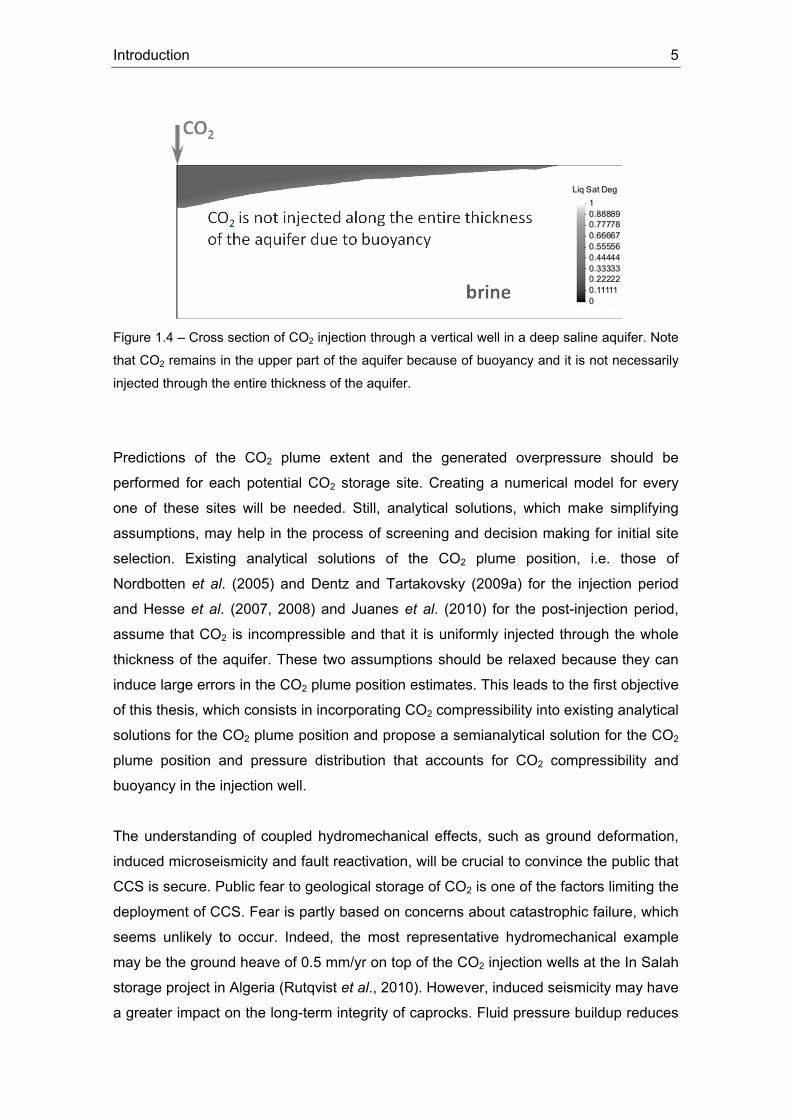
Buoyancy effects are rarely taken into account in the injection well. Instead, the well is
often simulated as a prescribed (constant) flux boundary. However, this boundary
condition plays a relevant role in determining the shape of the CO2 plume. Since CO2 is
buoyant with respect to the formation brine, CO2 tends to enter the aquifer
preferentially along the top portion of the aquifer (Figure 1.4). The CO2-brine interface
develops maintaining pressure equilibrium, i.e. CO2 pressure at the interface is equal to
brine pressure plus the capillary entry pressure. Thus, the plume will advance
according to pressure buildup. Aquifers with a high permeability offer low resistance to
CO2 advance. Therefore, the CO2 plume will advance preferentially through the top of
the aquifer, without occupying the whole thickness of the aquifer at the injection well. In
contrast, lower permeability aquifers experience a higher pressure buildup.
Consequently, the CO2 plume will also advance downwards inside the injection well
and may occupy the whole thickness of the aquifer at the injection well. Of course,
once the CO2 enters the aquifer, it will tend to flow upwards due to buoyancy.
Introduction 5
Figure 1.4 – Cross section of CO2 injection through a vertical well in a deep saline aquifer. Note
that CO2 remains in the upper part of the aquifer because of buoyancy and it is not necessarily
injected through the entire thickness of the aquifer.
Predictions of the CO2 plume extent and the generated overpressure should be
performed for each potential CO2 storage site. Creating a numerical model for every
one of these sites will be needed. Still, analytical solutions, which make simplifying
assumptions, may help in the process of screening and decision making for initial site
selection. Existing analytical solutions of the CO2 plume position, i.e. those of
Nordbotten et al. (2005) and Dentz and Tartakovsky (2009a) for the injection period
and Hesse et al. (2007, 2008) and Juanes et al. (2010) for the post-injection period,
assume that CO2 is incompressible and that it is uniformly injected through the whole
thickness of the aquifer. These two assumptions should be relaxed because they can
induce large errors in the CO2 plume position estimates. This leads to the first objective
of this thesis, which consists in incorporating CO2 compressibility into existing analytical
solutions for the CO2 plume position and propose a semianalytical solution for the CO2
plume position and pressure distribution that accounts for CO2 compressibility and
buoyancy in the injection well.
The understanding of coupled hydromechanical effects, such as ground deformation,
induced microseismicity and fault reactivation, will be crucial to convince the public that
CCS is secure. Public fear to geological storage of CO2 is one of the factors limiting the
deployment of CCS. Fear is partly based on concerns about catastrophic failure, which
seems unlikely to occur. Indeed, the most representative hydromechanical example
may be the ground heave of 0.5 mm/yr on top of the CO2 injection wells at the In Salah
storage project in Algeria (Rutqvist et al., 2010). However, induced seismicity may have
a greater impact on the long-term integrity of caprocks. Fluid pressure buildup reduces
6 Chapter 1
effective stresses, which induces straining of the rock and can eventually trigger
microseismic events. These can open fractures and reactivate faults, which might
create flow paths through which CO2 could migrate upwards. Furthermore, fault
reactivation could potentially trigger a seismic event that could be felt by the local
population (Cappa and Rutqvist, 2011b). A 3.4 magnitude injection induced seismic
event triggered in Basel, Switzerland, during the hydraulic stimulation of a geothermal
project motivated the shut-down of the project because of concerns by the local
community (Häring et al., 2008). However, important differences exist between a
geothermal stimulation and geologic CO2 storage: CO2 overpressure will be limited in
order to avoid the opening of fractures, while geothermal stimulation aims precisely to
open them; CO2 will be injected in aquifers, while geothermal projects usually take
place in low-permeability formations like granites. Hence, notable seismic events are
not likely to occur in geologic CO2 storage. Still, special attention has to be paid to
hydromechanical coupled processes to avoid undesired phenomena such as fault
reactivation, fracturing or well damage, which could lead to CO2 leakage.
Coupled hydromechanical models can aid in defining the maximum sustainable
injection pressure that guarantees that no CO2 leakage will occur (Rutqvist et al.,
2007). This maximum sustainable injection pressure coincides with the yield of the
rock, which triggers microseismic events. CO2 injection is intended to last for decades
(30 to 50 years), so the pressure buildup cone caused by injection will propagate over
large distances, reaching the boundaries of the aquifer. The nature of the boundary will
influence fluid pressure evolution, which may affect caprock stability. Therefore, the
second objective of this thesis is to understand fluid pressure evolution and how it is
affected by boundary conditions as well as to investigate induced stress and strain
(reversible and irreversible) during CO2 injection to assess caprock stability.
The mechanical properties of the rocks are usually measured at the laboratory from
core samples. However, the values that should be used in the models to reproduce the
hydromechanical behaviour at the field scale differ significantly from those obtained
from core samples (e.g. Verdon et al., 2011). This is mainly because rock masses
contain not only the rock matrix tested at the laboratory, but also fractures that are not
present in the cores. Therefore, field tests are needed to obtain representative values
of the rock mechanical properties, to define the maximum sustainable injection
pressure and to select suitable sequestration sites. The proposal of this test constitutes
the third objective of this thesis.

Introduction 7
Another issue of relevance is the way in which CO2 is injected into the reservoir. In
general, it is assumed that CO2 will be injected in supercritical state because the
pressure and temperature conditions of the target aquifers are such that CO2 will
remain in supercritical state. However, inflowing CO2 may not be in thermal equilibrium
with the aquifer because pressure and temperature injection conditions at the wellhead
can have a very broad range and CO2 will not equilibrate with the geothermal gradient
if the flow rate is high. Temperature differences induce stress changes that can affect
the mechanical stability of the caprock (Preisig and Prévost, 2011). This leads to the
need for non-isothermal simulations of CO2 injection in deformable porous media.
Furthermore, other injection strategies may present a lower probability of CO2 leakage
or reduce the costs of supercritical CO2 injection. For instance, pumping brine from the
aquifer to reduce the overpressure and reinject it saturated in CO2 avoids the presence
of CO2 in free phase and minimizes the risk of leakage because brine with dissolved
CO2 is denser than brine without CO2, thus sinking. Hence, injection strategies other
than the widely accepted supercritical CO2 injection should also be considered to
enhance proposed CCS projects. Thus, the final objective of this thesis is to propose a
new injection strategy that minimizes energy consumption and to assess the caprock
mechanical stability of this injection strategy considering thermo-hydro-mechanical
couplings.
1.2. Thesis layout
This Thesis is organized in seven chapters, which coincide with papers already
published in international scientific journals or in the process. Each chapter contains its
own introduction and conclusions. A common reference list is included at the end of the
document. The structure of the Thesis is as follows:
- Chapter 2 deals with the effects of CO2 compressibility on the prediction of the
CO2 plume position using existing analytical solutions; we present a correction
to account for CO2 compressibility in these analytical solutions. Fluid pressure is
derived from these analytical solutions. The results from the analytical solutions
are compared with numerical simulations. The contents of this chapter have
given rise to the publication of Vilarrasa et al. (2010a) in the scientific journal
Transport In Porous Media.
8 Chapter 1
- Chapter 3 presents a semianalytical solution for the CO2 plume position and
pressure evolution during injection of compressible CO2 considering buoyancy
effects in the injection well. The aquifer is discretized into horizontal layers
through which CO2 advances laterally and vertically downwards. CO2 is not
necessarily injected through the whole thickness of the aquifer because of its
buoyancy. The contents of this chapter have been presented in a conference
(Vilarrasa et al., 2010c) and it is planned to publish them in a scientific journal.
- Chapter 4 focuses on the hydromechanical coupling of CO2 sequestration in
deep saline aquifers and how pressure buildup affects the mechanical caprock
stability. Pressure evolution and the effect of the hydraulic boundary conditions
are analyzed. The contents of this chapter have already been published in
international scientific journals (Vilarrasa et al., 2010b; 2011b) and have been
presented in several conferences (Vilarrasa et al., 2009; 2010d, e, f, g; 2011e).
- Chapter 5 introduces a hydromechanical characterization test to assess the
suitability of CO2 injection sites to withstanding fluid pressure buildup. A
literature review of the mechanical properties of the rocks involved in CO2
sequestration is presented. The mechanical properties of the aquifer and
caprock can be estimated from introducing the field measurements of the test
(overpressure and vertical displacement) into the plots obtained from numerical
simulations expressed in dimensionless variables. The onset of microseismicity
defines the maximum sustainable injection pressure and microseismicity
evolution can give information on the stress regime. The contents of this
chapter have been presented in several conferences (Vilarrasa et al., 2011c, d;
2012a) and it is planned to publish them in a scientific journal.
- Chapter 6 proposes a new CO2 injection concept which consists in injecting
CO2 in liquid state. Injecting liquid CO2 reduces fluid overpressure and improves
caprock stability. To analyze this, simulations of non-isothermal two-phase flow
in a deformable media are performed. The coupled thermo-hydro-mechanical
processes occurring when injecting cold CO2 are investigated. The contents of
this chapter have been presented in several conferences (Vilarrasa et al.,
2012b, c, d) and it is planned to publish them in a scientific journal.
- Chapter 7 provides some general conclusions withdrawn from the previous
chapters.
9
2. Effects of CO2 Compressibility on
CO2 Storage in Deep Saline
Aquifers
2.1. Introduction
Carbon dioxide (CO2) sequestration in deep geological formations is considered a
promising mitigation solution for reducing greenhouse gas emissions to the
atmosphere. Although this technology is relatively new, wide experience is available in
the field of multiphase fluid injection (e.g. the injection of CO2 for enhanced oil recovery
(Lake, 1989; Cantucci et al., 2009), production and storage of natural gas in aquifers
(Dake, 1978; Katz and Lee, 1990), gravity currents (Huppert and Woods, 1995; Lyle et
al., 2005) and disposal of liquid waste (Tsang et al., 2008)). Various types of geological
formations can be considered for CO2 sequestration. These include unminable coal
seams, depleted oil and gas reservoirs and deep saline aquifers. The latter have
received particular attention due to their high CO2 storage capacity (Bachu and Adams,
2003). Viable saline aquifers are typically at depths greater than 800 m. Pressure and
temperature conditions in such aquifers ensure that the density of CO2 is relatively high
(Hitchon et al., 1999).
Several sources of uncertainty associated with multiphase flows exist at these depths.
These include those often encountered in other subsurface flows such as the impact of
heterogeneity of geological media, e.g. (Neuweiller et al., 2003; Bolster et al., 2009b),
variability and lack of knowledge of multiphase flow parameters (e.g. van Genuchten
and Brooks-Corey models). Beyond these difficulties, the properties of supercritical
CO2, such as density and viscosity, can vary substantially (Garcia, 2003; Garcia and
Pruess, 2003; Bachu, 2003) making the assumption of incompressibility questionable.
Two analytical solutions have been proposed for the position of the interface between
the CO2 rich phase and the formation brine: the Nordbotten et al. (2005) solution and
10 Chapter 2
the Dentz and Tartakovsky (2009a) solution. Both assume an abrupt interface between
phases. Both solutions neglect CO2 dissolution into the brine, so the effect of
convective cells (Ennis-king and Paterson, 2005; Hidalgo and Carrera, 2009; Riaz et
al., 2006) on the front propagation is not taken into account. Each phase has constant
density and viscosity. The shape of the solution by Nordbotten et al. (2005) depends on
the viscosity of both CO2 and brine, while the one derived by Dentz and Tartakovsky
(2009a) depends on both the density and viscosity differences between the two
phases. The validity of these sharp interface solutions has been discussed in, e.g.,
Dentz and Tartakovsky (2009a, b); Lu et al. (2009).
The injection of CO2 causes an increase in fluid pressure and displaces the formation
brine laterally. This brine can migrate out of the aquifer if the aquifer is open, causing
salinization of other formations such as fresh water aquifers. In contrast, if the aquifer
has very low-permeability boundaries, the storage capacity will be related exclusively to
rock and fluid compressibility (Zhou et al., 2008). In the latter case, fluid pressure will
increase dramatically and this can lead to geomechanical damage of the caprock
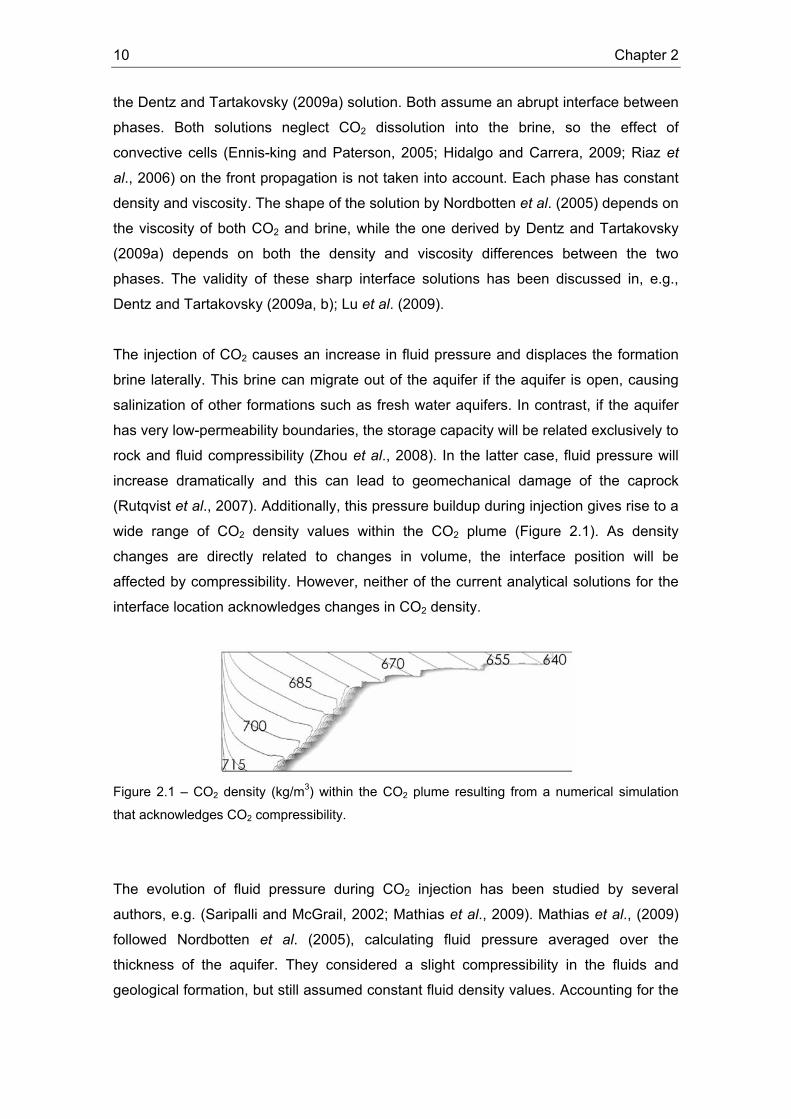
(Rutqvist et al., 2007). Additionally, this pressure buildup during injection gives rise to a
wide range of CO2 density values within the CO2 plume (Figure 2.1). As density
changes are directly related to changes in volume, the interface position will be
affected by compressibility. However, neither of the current analytical solutions for the
interface location acknowledges changes in CO2 density.
Figure 2.1 – CO2 density (kg/m3) within the CO2 plume resulting from a numerical simulation
that acknowledges CO2 compressibility.
The evolution of fluid pressure during CO2 injection has been studied by several
authors, e.g. (Saripalli and McGrail, 2002; Mathias et al., 2009). Mathias et al., (2009)
followed Nordbotten et al. (2005), calculating fluid pressure averaged over the
thickness of the aquifer. They considered a slight compressibility in the fluids and
geological formation, but still assumed constant fluid density values. Accounting for the
CO2 Compressibility Effects 11
slight compressibility allows them to avoid the calculation of the radius of influence,
which, as we propose later, can be determined by Cooper and Jacob (1946) method.
Typically CO2 injection projects are intended to take place over several decades. This
implies that the radius of the final CO2 plume, which can be calculated with the above
analytical solutions (Stauffer et al., 2009), may reach the kilometer scale. The omission
of compressibility effects can result in a significant error in these estimates. This in turn
reduces the reliability of risk assessments, where even simple models can provide a lot
of useful information (e.g. Tartakovsky (2007); Bolster et al. (2009a)).
The nature of uncertainty in the density field is illustrated by the Sleipner Project
(Korbol and Kaddour, 1995). There, around one million tons of CO2 have been injected
annually into the Utsira formation since 1996. Nooner et al. (2007) found that the best
fit between the gravity measurements made in situ and models based on time-lapse 3D
seismic data corresponds to an average in situ CO2 density of 530 kg/m3, with an
uncertainty of ±65 kg/m3. This uncertainty is significant in itself. However, prior to these
measurements and calculations, the majority of the work on the site had assumed a
range between 650-700 kg/m3, which implies a significant error (> 20 %) in volume
estimation.
Here we study the impact of CO2 compressibility on the interface position, both
numerically and analytically. We propose a simple method to account for
compressibility effects (density variations) and viscosity variations and apply it to the
analytical solutions of Nordbotten et al. (2005) and Dentz and Tartakovsky (2009a).
First, we derive an expression for the fluid pressure distribution in the aquifer from the
analytical solutions. Then, we propose an iterative method to determine the interface
position that accounts for compressibility. Finally, we contrast these corrections with
the results of numerical simulations and conclude with a discussion on the importance
of considering CO2 compressibility in the interface position.
2.2. Multiphase flow. The role of compressibility
Consider injection of supercritical CO2 in a deep confined saline aquifer (see a
schematic description in Figure 2.2). Momentum conservation is expressed using
Darcy's law, which for phases CO2, c, and brine, w, is given by

12 Chapter 2
( ) wczgPkkr , , =∇+∇−= αρμ ααα
ααq , (2.1)
where αq is the volumetric flux of α ‐phase, k is the intrinsic permeability, αrk is the
α -phase relative permeability, αμ its viscosity, αP its pressure, αρ its density, g is
gravity and z is the vertical coordinate.
Figure 2.2 – Problem setup. Injection of compressible CO2 in a homogeneous horizontal deep
saline aquifer.
Mass conservation of these two immiscible fluids can be expressed as (Bear, 1972),
( ) ( ) wctS , , =⋅−∇=∂
∂ αρϕραα
αα q , (2.2)
where αS is the saturation of the α -phase, ϕ is the porosity of the porous medium
and t is time.
The left-hand side of Eq. (2.2) represents the time variation of the mass of α -phase
per unit volume of porous medium. Assuming that there is no external loading, and that
the grains of the porous medium are incompressible, but not stationary (Bear, 1972),
the expansion of the partial derivative of this term results in
( )tS
tPcS
tPcS
tS
r ∂∂
+∂∂
+∂∂
=∂
∂ αα
ααα
αααα
αα ϕρρϕρϕρ, (2.3)
where ( )( )αααα ρρ Pc d/d/1= is fluid compressibility, σε ′= /dd vrc is rock compressibility, vε
is the volumetric strain and σ ′ is the effective stress.
The first term in the right-hand side of Eq. (2.3) corresponds to changes in storage
caused by the compressibility of fluid phases. The second term refers to rock
CO2 Compressibility Effects 13
compressibility. The third term in the right-hand side of Eq. (2.3) represents changes in
the mass of α caused by fluid saturation-desaturation processes (i.e., CO2 plume
advance). As such, it does not represent compressibility effects, although its actual
value will be sensitive to pressure through the phase density, which controls the size of
the CO2 plume.
The relative importance of the first two terms depends on whether we are in the CO2 or
brine zones, because the compressibility of CO2 is much larger than that of brine and
rock. Typical rock compressibility values at depths of interest for CO2 sequestration
range from 10-11 to 5·10-9 Pa-1 (Neuzil, 1986), but can be effectively larger if plastic
deformation conditions are reached. Water compressibility is of the order of 4.5·10-10
Pa-1, which lies within the range of rock compressibility values. CO2 compressibility
ranges from 10-9 to 10-8 Pa-1 (Law and Bachu, 1996; Span and Wagner, 1996), one to
two orders of magnitude greater than that of rock and water. Thus, CO2 compressibility
has a significant effect on the first term in the right-hand side of Eq. (2.3). However, the
second term, which accounts for rock compressibility, can be neglected in the CO2 rich
zone, both because it is small and because the volume of rock occupied by CO2 is
orders of magnitude smaller than that affected by pressure buildup of the formation
brine.
The situation is different in the region occupied by resident water. Water compressibility
is at the low end of rock compressibilities at large depths. Moreover, its value is
multiplied by porosity. Therefore, water compressibility will only play a relevant role in
high porosity stiff rocks, which are rare. In any case, the two compressibility terms can
be combined in the brine saturated zone, yielding
( )thS
thccg w
sw
rww ∂∂
=∂∂
+ϕρ , (2.4)
where wh is the hydraulic head of water, sS is the specific storage coefficient (Bear,
1972), which accounts for both brine and rock compressibility.
The specific storage coefficient controls, together with permeability, the radius of
influence, R (i.e. the size of the pressure buildup cone caused by injection). In fact,
assuming the aquifer to be large and for the purpose of calculating pressure buildup,
this infinite compressible system can be replaced by an incompressible system whose
radius grows as determined from the comparison between Thiem's solution (steady
state) (Thiem, 1906) and Jacob's solution (transient) (Cooper and Jacob, 1946)
14 Chapter 2
⎟⎟⎠
⎞⎜⎜⎝
⎛=⎟⎟
⎠
⎞⎜⎜⎝
⎛=Δ
sw
wwww Sr
gtkkd
QrR
kdQP 2
02
20 25.2ln
4ln
4 μρ
πμ
πμ
, (2.5)
where 0Q is the volumetric flow rate, d is the aquifer thickness and r is radial
distance. The radius of influence can then be defined from Eq. (2.5) as
sw
w
SgtkR
μρ25.2
= . (2.6)
CO2 is lighter than brine and density differences affect flow via buoyancy. To quantify
the relative influence of buoyancy we define a gravity number, N , as the ratio of
gravity to viscous forces. The latter can be represented by the horizontal pressure
gradient ( )2/(0 krdQ πμ ), and the former by the buoyancy force ( g ρΔ ) in Darcy's law,
expressed in terms of equivalent head. This would yield the traditional gravity number
for incompressible flow (e.g. Lake, 1989). However, for compressible fluids, the
boundary condition is usually expressed in terms of the mass flow rate, mQ (Figure
2.2). Therefore, it is more appropriate to write 0Q as ρ/mQ . Hence, N becomes
mc
cc
QdrgkN
μρρπ Δ
=2
, (2.7)
where cw ρρρ −=Δ is the difference between the fluid densities, cρ is a characteristic
density, cr is a characteristic length and mQ is the CO2 mass flow rate. Large gravity
numbers (N >> 1) indicate that gravity forces dominate. Small gravity numbers ( N <<
1) indicate that viscous forces dominate. Gravity numbers close to one indicate that
gravity and viscous forces are comparable.
The characteristic density can be chosen as the mean CO2 density of the plume. The
characteristic length depends on the scale of interest (Kopp et al., 2009). The gravity
number increases with the characteristic length, thus increasing the relative importance
of gravity forces with respect to viscous forces (Tchelepi and Orr Jr., 1994). This
implies that, as the CO2 plume becomes large, gravity forces will dominate far from the
injection well.
These equations can be solved numerically (e.g. Aziz and Settari, 2002; Chen et al.,
2006; Pruess et al., 2004). However, creating a numerical model for each potential
candidate site may require a significant cost. Alternatively, the problem can be solved
analytically using some simplifications. The use of analytical solutions is useful
because (i) they are instantaneous (Stauffer et al., 2009), (ii) numerical solutions can
CO2 Compressibility Effects 15
be coupled with analytical solutions to make them more efficient (Celia and Nordbotten,
2009) and (iii) they identify important scaling relationships that give insight into the
balance of the physical driving mechanisms.
2.3. Analytical solutions
2.3.1. Abrupt interface approximation The abrupt interface approximation considers that the two fluids, CO2 and brine in this
case, are immiscible and separated by a sharp interface. The saturation of each fluid is
assumed constant in each fluid region and capillary effects are usually neglected.
Neglecting compressibility and considering a quasi-steady (successive steady-states)
description of moving fronts in Eq. (2.2) yields that the volumetric flux defined in (2.1) is
divergence free. Additionally, if the Dupuit assumption is adopted in a horizontal radial
aquifer and αS is set to 1, i.e. the α -phase relative permeability equals 1, the following
equation can be derived (Bear, 1972)
( )( )( ) 02
///21 0 =
∂∂
+⎥⎦
⎤⎢⎣
⎡−+
∂∂−Δ−∂∂
tdrdkgrQ
rr cw
c ςπϕμμςς
ςςμρπς , (2.8)
where ς is the distance from the base of the aquifer to the interface position. To
account for a residual saturation of the formation brine, rwS , behind the CO2 front, one
should replace cμ by rcc k′/μ in Eq. (2.8) and below, where rck′ is the CO2 relative
permeability evaluated at the residual brine saturation rwS . Equation (2.8) can be
expressed in dimensionless form using
, ,// , , , N
kkM
ttt
rrr
crc
wrw
cD
cD
cD μ
μςςς ==== (2.9)
where M is the mobility ratio, N is the gravity number defined in Eq. (2.7), ct is the
characteristic time and the subscript D denotes a dimensionless variable, which yields
( )( )( ) 0
/1/1/11
=∂∂
+⎥⎦
⎤⎢⎣
⎡−+
∂∂−−∂∂
D
D
DD
DDDcDD
DD tMrrdNr
rrς
ςςςςς . (2.10)
Equation (2.10) shows that the problem depends on two parameters, N and M . The
mobility ratio will have values around 0.1 for CO2 sequestration, which will lead to the
formation of a thin layer of CO2 along the top of the aquifer (Hesse et al., 2007, 2008;
Juanes et al., 2010). On the other hand, the gravity number can vary over several
16 Chapter 2
orders of magnitude, depending on the aquifer permeability and the injection rate.
Thus, the gravity number is the key parameter governing the interface position.
The analytical solutions of Nordbotten et al. (2005) and Dentz and Tartakovsky (2009a)
to determine the interface position of the CO2 plume when injecting supercritical CO2 in
a deep saline aquifer start from this approximation.
2.3.2. Nordbotten et al. (2005) approach To find the interface position, Nordbotten et al. (2005) solve Eq. (2.8) neglecting the
gravity term and approximating the transient system response to injection into an
infinite aquifer by a solution to the steady-state problem with a moving outer boundary
whose location increases in proportion to t in a radial geometry, i.e. the radius of
influence defined in (2.6). In addition, they impose (i) volume balance, (ii) gravity
override (CO2 plume travels preferentially along the top) and (iii) they minimize energy
at the well. The fluid pressure applies over the entire thickness of the aquifer and fluid
properties are vertically averaged. The vertically averaged properties are defined as a
linear weighting between the properties of the two phases. Nordbotten et al. (2005)
write their solution as a function of the mobility, αλ , defined as the ratio of relative
permeability to viscosity, ααα μλ /rk= . For the case of an abrupt interface where both
sides of the interface are fully saturated with the corresponding phase, the relative
permeability is 1 and αλ becomes the inverse of the viscosity of each phase. These
viscosities are assumed constant.
Under these assumptions, Nordbotten et al. (2005) obtain the interface position as,
( ) ( )⎥⎥⎦
⎤
⎢⎢⎣
⎡⎟⎟⎠
⎞⎜⎜⎝
⎛−
Δ−= 11, 2dr
tVdtrc
w
w
cN ϕπμ
μμμς , (2.11)
where ( ) tQtV ⋅= 0 is the CO2 volume assuming a constant CO2 density and
cw μμμ −=Δ is the difference between fluid viscosities.
Integrating the flow equation and assuming vertically integrated properties of the fluid
over the entire thickness of the formation, Nordbotten et al. (2005) provide the following
expression for fluid pressure buildup

CO2 Compressibility Effects 17
( ) ( ) ( )( )[ ]∫ +−Δ=−
R
r c
wN drdr
rk
QPtrPςμμπ
μ/
d2
, 00 , (2.12)
where NP is the vertically averaged pressure and 0P is the vertically averaged initial
pressure prior to injection.
2.3.3. Dentz and Tartakovsky (2009a) approach Dentz and Tartakovsky (2009a) also consider an abrupt interface approximation. They
include buoyancy effects, and the densities and viscosities of each phase are assumed
constant.
They combine Darcy's law with the Dupuit assumption in radial coordinates. Imposing
fluid pressure continuity at the interface they obtain
( ) ( )⎟⎟⎠
⎞⎜⎜⎝
⎛=
trrdtrb
cwDT ln, γς , (2.13)
where br is the radius of the interface at the base of the aquifer and cwγ is a
dimensionless parameter that measures the relative importance of viscous and gravity
forces
ρμ
πγ
ΔΔ
=gkd
Qcw 2
0
2. (2.14)
The interface radius at the base of the aquifer is obtained from volume balance as
( )1
0 12exp2−
⎥⎦
⎤⎢⎣
⎡−⎟⎟
⎠
⎞⎜⎜⎝
⎛=
cwcwb d
tQtrγγπϕ
. (2.15)
Note that the fluid viscosity contrast is treated differently in the two approaches (i.e.
mobility ratio and viscosity difference). The mobility ratio is particularly relevant in
multiphase flow when the two phases coexist. However, when one phase displaces the
other, the viscosity difference governs the process (see Eq. (2.14) in Dentz and
Tartakovsky (2009a) solution). An exception to this is the case when fluid properties
are integrated vertically (Nordbotten et al., 2005), which can be thought of as a
coexistence of phases.
18 Chapter 2
2.4. Compressibility correction
Let us assume that we have an initial estimation of the mean CO2 density and viscosity.
With this we can calculate the interface position using either analytical solutions (2.11)
or (2.13). Furthermore, the fluid pressure can be calculated from Darcy's law. Then, the
density can be determined within the plume assuming that it is solely a function of
pressure. Integrating the CO2 density within the plume and dividing it by the volume of
the plume, we obtain the mean CO2 density
( )( )
∫ ∫=d r
ccc zrPrV 0 0
dd21 ς
ρπϕρ , (2.16)
where V is the volume occupied by the CO2 plume and ( )ςr is the distance from the
well to the interface position from either Nordbotten et al. (2005) or Dentz and
Tartakovsky (2009a).
Note here that we do not specify a priori a particular relationship between density and
pressure. We only specify that density is solely a function of pressure. CO2 density also
depends on temperature (Garcia, 2003). However, we neglect thermal effects within
the aquifer, and take the mean temperature of the aquifer as representative of the
system. This assumption is commonly used in CO2 injection simulations (e.g. Law and
Bachu, 1996; Pruess and Garcia, 2002) and may be considered valid if CO2 does not
expand rapidly. If this happens, CO2 will experience strong cooling due to the Joule-
Thomson effect.
The relationship between pressure and density in Eq. (2.16) is in general nonlinear.
Moreover, pressure varies in space. Notice that the dependence is two-way: CO2
density depends explicitly on fluid pressure, but fluid pressure also depends on density,
because density controls the plume volume, and thus the fluid pressure through the
volume of water that needs to be displaced. Therefore, an iterative scheme is needed
to solve this nonlinear problem. As density varies moderately with pressure, a Picard
algorithm should converge, provided that the initial approximation is not too far from the
solution.
The formulation of this iterative approach requires an expression for the spatial
variability of fluid pressure for each of the two analytical solutions. In the approach of
Nordbotten et al. (2005), we obtain an expression for the vertically averaged pressure
by introducing (2.11) into (2.12) and integrating. The expression for pressure depends
CO2 Compressibility Effects 19
on the region: close to the injection well, all fluid is CO2; far away, all fluid is saline
water; in between the two phases coexist with an abrupt interface between them,
( )
( ) ( )( )
( ) ( )( ) ,lnln2
, ;
,ln2
, ;
,ln2
, ;
00
000
000
⎥⎦
⎤⎢⎣
⎡⎟⎠⎞
⎜⎝⎛+−+⎟
⎠⎞
⎜⎝⎛+=<
⎥⎦
⎤⎢⎣
⎡−+⎟
⎠⎞
⎜⎝⎛+=≤≤
⎟⎠⎞
⎜⎝⎛+=>
rrrr
tVd
rR
kdQPtrPrr
rrtVd
rR
kdQPtrPrrr
rR
kdQPtrPrr
b
w
cbo
w
cwNb
ow
cwNb
wN
μμ
μϕπμ
πμ
μϕπμ
πμ
πμ
(2.17)
where 0r is the radial distance where the interface intersects the top of the aquifer, br
is the radial distance where the interface intersects the bottom of the aquifer,
2/00 gdPP wt ρ+= is the vertically averaged fluid pressure prior to injection, and 0tP is
the initial pressure at the top of the aquifer. Mathias et al. (2009) come to a similar
expression for fluid pressure, but they consider a slight compressibility in the fluids and
rock instead of a radius of influence. The vertically averaged fluid pressure varies with
the logarithm of the distance to the well in the regions where a single phase is present
(CO2 or brine). However, it varies linearly in the region where both phases coexist.
Fluid pressure can be obtained from the Dentz and Tartakovsky (2009a) approach by
integrating (2.1), assuming hydrostatic pressure (Dupuit approximation) in the aquifer,
and taking the interface position given by (2.13), which yields
( ) ( ) ( )
( ) ( ) ( )
.lnln2
,, ;
,ln2
,, ;
0
0
00
⎥⎦
⎤⎢⎣
⎡Δ−⎟
⎠⎞
⎜⎝⎛+⎟⎟
⎠
⎞⎜⎜⎝
⎛+
−+=≤
⎟⎠⎞
⎜⎝⎛+−+=>
cw
bc
bw
wtDTDT
wwtDTDT
dz
rr
rR
kdQ
zdgPtzrPrrrR
kdQzdgPtzrPrr
γμμμ
π
ρςπμρς
(2.18)
Equation (2.18) can be averaged over the entire thickness of the aquifer to obtain an
averaged pressure, which will be used to compare the two approaches. This averaged
pressure is given by
20 Chapter 2
( )
( )
( ) .2
lnln2
, ;
,ln12
ln1ln
lnlnln2
, ;
,ln2
, ;
00
2
2
000
000
⎥⎦
⎤⎢⎣
⎡ Δ−⎟
⎠⎞
⎜⎝⎛+⎟⎟
⎠
⎞⎜⎜⎝
⎛+=<
⎪⎭
⎪⎬⎫
⎥⎥⎦
⎤
⎢⎢⎣
⎡
⎟⎟⎠
⎞⎜⎜⎝
⎛⎟⎟⎠
⎞⎜⎜⎝
⎛−
Δ−
⎥⎦
⎤⎢⎣
⎡⎟⎟⎠
⎞⎜⎜⎝
⎛−⎟
⎠⎞
⎜⎝⎛+
⎪⎩
⎪⎨⎧
⎥⎦
⎤⎢⎣
⎡⎟⎠⎞
⎜⎝⎛
⎟⎟⎠
⎞⎜⎜⎝
⎛+⎟⎟
⎠
⎞⎜⎜⎝
⎛+=≤≤
⎟⎠⎞
⎜⎝⎛+=>
cw
bc
bwDTb
bcw
cw
bcw
bc
b
bcw
bwDTb
wDT
rr
rR
kdQPtrPrr
rr
rr
rr
rr
rr
rR
kdQPtrPrrr
rR
kdQPtrPrr
γμμμ
π
γγμ
γμ
γμπ
πμ
(2.19)
Thus, the vertically averaged fluid pressure is defined in three regions in both
approaches by Eqs. (2.17) and (2.19). Unsurprisingly, the two approaches have the
same solution in the regions where only one phase exists. Differences appear in the
region where CO2 and the formation brine coexist. In the Nordbotten et al. (2005)
approach, the vertically averaged pressure varies linearly with distance to the well.
However, in Dentz and Tartakovsky (2009a), it changes logarithmically with distance to
the well. As a result, the approach of Dentz and Tartakovsky (2009a) predicts higher
fluid pressure values in this zone.
Equations (2.17) and (2.18) allow us to develop a simple iterative method for correcting
the interface position. The method can be applied to both the Nordbotten et al. (2005)
and Dentz and Tartakovsky (2009a) solutions as well as to any other future solutions
that may emerge. The procedure is as follows
1) Take a reasonable initial approximation for mean CO2 density and viscosity
from the literature, e.g. Bachu (2003).
2) Determine the interface position using mean density and viscosity in analytical
solutions (2.11) or (2.13).
3) Calculate the pressure distribution using (2.17) or (2.18).
4) Calculate the corresponding mean density and viscosity of the CO2 using (2.16).
5) Repeat steps 2-4 until the solution converges to within some prespecified
tolerance. Two different convergence criteria can be chosen: (i) changes in the
interface position or (ii) changes in the mean CO2 density.
CO2 Compressibility Effects 21
The method is relatively easy to implement and can be programmed in a spreadsheet
or any code of choice. The method converges rapidly, within a few iterations (typically
less than 5) in all test cases. A calculation spreadsheet can be downloaded from GHS
(2009).
2.5. Application
2.5.1. Injection scenarios To illustrate the relevance of CO2 compressibility effects, we consider three injection
scenarios: (i) a regime in which viscous forces dominate gravity forces, (ii) one where
both forces have a similar influence and (iii) a case where gravity forces dominate.
CO2 thermodynamic properties have been widely investigated (e.g. Sovova and
Prochazka, 1993; Span and Wagner, 1996; Garcia, 2003). The thermodynamic
properties given by Span and Wagner (1996) are almost identical to the International
Union of Pure and Applied Chemistry (IUPAC) (Angus et al., 1976) data sets over the
P-T range of CO2 sequestration interest (McPherson et al., 2008). However, the
algorithm given by Span and Wagner (1996) for evaluating CO2 properties has a very
high computational cost. For the sake of simplicity and illustrative purposes, we
assume a linear relationship between CO2 density and pressure, given as
( )010 tcc PP −+= βρρρ , (2.20)
where 0ρ and 1ρ are constants for the CO2 density, β is CO2 compressibility, cP is
CO2 pressure and 0tP is the reference pressure for 0ρ . 0ρ , 1ρ and β are obtained
from data tables in Span and Wagner (1996). Appendix I contains the expressions for
the mean CO2 density using this linear approximation in (2.20) for both approaches.
CO2 viscosity is calculated using an expression proposed by Altunin and
Sakhabetdinov (1972). In this expression, the viscosity is a function of density and
temperature. Thus the mean CO2 viscosity is calculated from the mean CO2 density.
Figure 2.3 shows how the density varies within the CO2 plume for one of our numerical
simulations. The numerical simulations calculate CO2 density assuming the Redlich-
Kwong equation of state (Redlich and Kwong, 1949) using the parameters for CO2
proposed by Spycher et al. (2003) and CO2 viscosity using the expression of Altunin
and Sakhabetdinov (1972) (see Appendix II). The maximum error encountered in this

22 Chapter 2
study due to the linear CO2 density approximation was around 8 %, which we deem
acceptable for our illustrative purposes. Bachu (2003) shows vertical profiles of CO2
density assuming hydrostatic pressure and different geothermal gradients. However,
pressure buildup affects CO2 properties. Hence, these vertical profiles can only be
taken as a reference, for example, to obtain the initial approximation of CO2 density
and viscosity.
500
600
700
11
12
13
14
15
0 500 1000
Den
sity
(kg/m
3 )
P c(M
Pa)
r (m)
Pc
ρc
Figure 2.3 – CO2 pressure and CO2 density at the top of the aquifer resulting from a numerical
simulation that acknowledges CO2 compressibility.
We study a saline aquifer at a depth that ranges from 1000 to 1100 m. The
temperature is assumed to be constant and equal to 320 K. For this depth and
temperature, the initial CO2 density is estimated as 730 kg/m3 (Bachu, 2003). The
corresponding CO2 viscosity according to Altunin and Sakhabetdinov (1972) is 0.061
mPa·s.
For the numerical simulations we used the program CODE_BRIGHT (Olivella et al.,
1994; 1996) with the incorporation of the above defined constitutive equations for CO2
density and viscosity. This code solves the mass balance of water and CO2 (Eq. (2.2))
using the Finite Element Method and a Newton-Raphson scheme to solve the
nonlinearities. The aquifer is represented by an axisymmetric model in which a
constant CO2 mass rate is injected uniformly in the whole vertical of a well with radius,
pr , 0.15 m. The aquifer is assumed infinite-acting, homogeneous and isotropic. In
order to obtain a solution close to an abrupt interface, a van Genuchten retention curve
(van Genuchten, 1980), with an entry pressure, ccP , of 0.02 MPa and the shape
CO2 Compressibility Effects 23
parameter m =0.8, was used. To approximate a sharp interface, linear relative
permeability functions, for both the CO2 and the brine, have been used (Table 2.1).
This retention curve and relative permeability functions enable us to obtain a CO2 rich
zone with a saturation very close to 1, and a relatively narrow mixing zone. The CO2
saturation 90 % isoline has been chosen to represent the position of the interface.
Table 2.1 – Parameters considered for the numerical simulations in the three injection scenarios.
m ccP (MPa) k (m2) αrk mQ (kg/s) pr (m) sS
Case 1 10-13 120
Case 2 0.8 0.02 10-12 αrS 79 0.15 1.76·10-6
Case 3 10-12 1
2.5.2. Case 1: Viscous forces dominate This first case consists of an injection with a gravity number of the order of 10-3 in the
well. In this situation, the corrected mean CO2 density (770 kg/m3 for Nordbotten et al.
(2005) and 803 kg/m3 for Dentz and Tartakovsky (2009a)) is higher than that assumed
initially (730 kg/m3). The corresponding CO2 viscosities are 0.067 and 0.073 mPa·s
respectively. Therefore, the corrected interface position is located closer to the well
than when we neglect variations in density. The Dentz and Tartakovsky (2009a)
approach gives a higher value of the mean CO2 density because fluid pressure grows
exponentially, while it grows linearly in Nordbotten et al. (2005) approach, thus leading
to lower fluid pressure values in the zone where CO2 and brine coexist. We define
relative error, relE , of the interface position as
i
cirel R
RRE −= , (2.21)
where iR is the radius of the CO2 plume at the top of the aquifer for incompressible
CO2 and cR is the radius of the CO2 plume at the top of the aquifer for compressible
CO2.
Differences between the compressible and incompressible solutions are shown in
Figure 2.4. For the Dentz and Tartakovsky (2009a) solution, the relative error increases
slightly from the base to the top of the aquifer, presenting a maximum relative error of 6
% at the top of the aquifer. For the Nordbotten et al. (2005) solution the interface tilts,
with the base of the interface located just 2 % further from the well than its initial
24 Chapter 2
position, but the top positioned 7 % closer to the well. The difference in shape between
the two analytical solutions results in a CO2 plume that extends further along the top of
the aquifer for Nordbotten et al. (2005) solution than Dentz and Tartakovsky (2009a)
over time (Figure 2.4b). A similar behaviour can be seen in the numerical simulations
(Figure 2.4a). In this case, the interface given by the numerical simulation compares
favourably with that of Nordbotten et al. (2005).
Figure 2.4c displays a comparison between the vertically averaged fluid pressure given
by both approaches. The fluid pressure given by Mathias et al. (2009) is identical to
that obtained in Nordbotten et al. (2005) approach (Eq. (2.17)). This is because
Mathias et al. (2009) assumed the Nordbotten et al. (2005) solution for the interface
position and that the hypothesis made therein are valid. Thus, both expressions can be
considered equivalent for the vertically averaged fluid pressure. Fluid pressure
obtained from the numerical simulation is smaller than the other profiles inside the CO2
plume region. This may reflect the larger energy dissipation produced by analytical
solutions as a result of the Dupuit assumption.
2.5.3. Case 2: Comparable gravity and viscous forces Here, the gravity number at the well is in the order of 10-1 (Note that the gravity number
increases to 1 if we take a characteristic length only 1.5 m away from the injection well.
In fact, it keeps increasing further away from the well, where gravity forces will
eventually dominate (recall Section 3)). The density variations between the initial guess
of 730 kg/m3 and the corrected value can be large. The density reduces to 512 kg/m3
(viscosity of 0.037 mPa·s) for Nordbotten et al. (2005) and to 493 kg/m3 (viscosity of
0.036 mPa·s) for Dentz and Tartakovsky (2009a). This means that the error associated
with neglecting CO2 compressibility can become very large and should be reflected in
the interface position (Figure 2.5a). For the Dentz and Tartakovsky (2009a) solution
including compressibility leads to a 26 % error at the top of the aquifer. This relative
error reaches 53 % in the Nordbotten et al. (2005) solution. Over a 30 year injection
this could represent a potential error of 3 km in the interface position estimation (Figure
2.5b). Here, the numerical simulations also show the importance of considering CO2
compressibility. The interface position from the simulations is similar to that of
Nordbotten et al. (2005) in the lower half of the aquifer, where viscous forces may
dominate, but it is similar to that of Dentz and Tartakovsky (2009a) in the upper part of
the aquifer, where buoyancy begins to dominate.

CO2 Compressibility Effects 25
0
25
50
75
100
0 250 500 750
z(m
)
r (m)
IncompressibleCompressible
DT
NOCB
(a)
0
2
4
6
8
0 10 20 30
r 0(km)
t (yr)
Incompressible
Compressible
DT
NO
CB
(b)
Figure 2.4 – Case 1: Viscous forces dominate. Gravity number, N , equals 10-3 in the well. (a)
Abrupt interface position in a vertical cross section after 100 days of injection, (b) evolution of
the CO2 plume radius at the top of the aquifer and (c) vertically averaged fluid pressure with
distance to the well after 100 days of injection, with a detail of the CO2 rich zone. NO refers to
Nordbotten et al. (2005) solution, DT to Dentz and Tartakovsky (2009a) solution, CB to the
numerical solution of CODE_BRIGHT and M is the Mathias et al. (2009) solution for fluid
pressure.
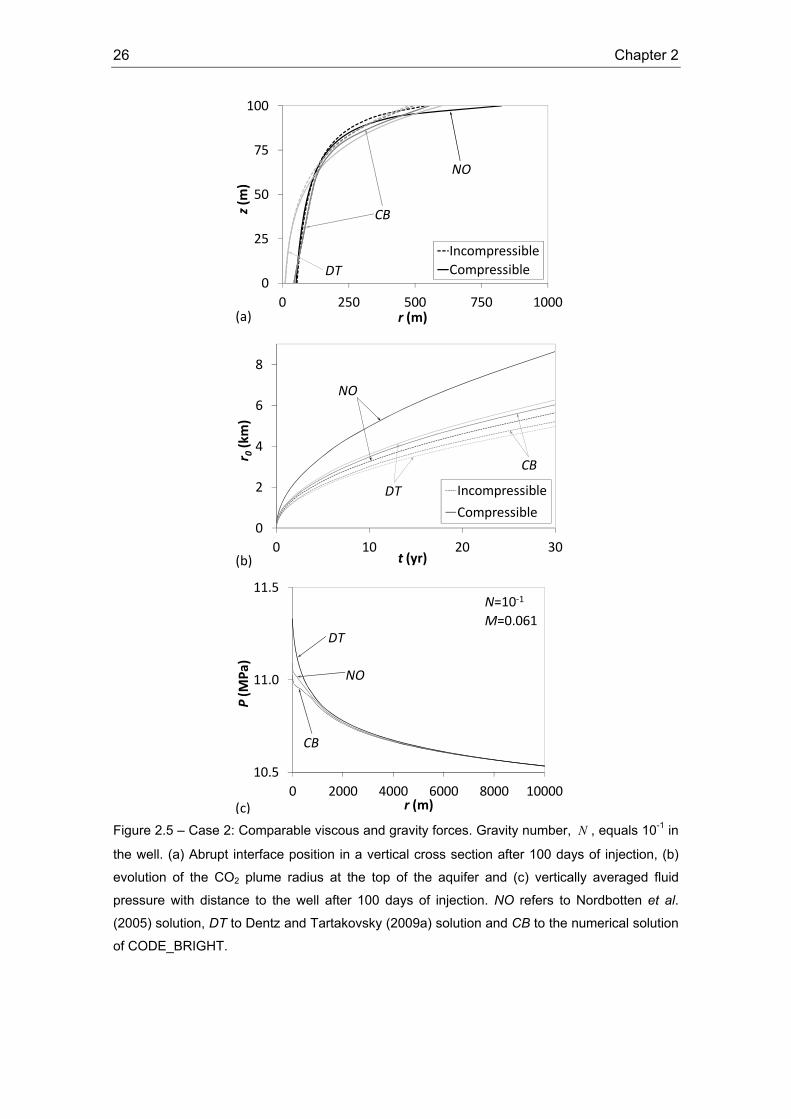
26 Chapter 2
0
25
50
75
100
0 250 500 750 1000
z(m
)
r (m)
IncompressibleCompressible
NO
CB
DT
(a)
0
2
4
6
8
0 10 20 30
r 0(km)
t (yr)
Incompressible
Compressible
DT
NO
CB
(b)
10.5
11.0
11.5
0 2000 4000 6000 8000 10000
P(M
Pa)
r (m)
DT
NO
CB
(c)
N=10‐1
M=0.061
Figure 2.5 – Case 2: Comparable viscous and gravity forces. Gravity number, N , equals 10-1 in
the well. (a) Abrupt interface position in a vertical cross section after 100 days of injection, (b)
evolution of the CO2 plume radius at the top of the aquifer and (c) vertically averaged fluid
pressure with distance to the well after 100 days of injection. NO refers to Nordbotten et al.
(2005) solution, DT to Dentz and Tartakovsky (2009a) solution and CB to the numerical solution
of CODE_BRIGHT.
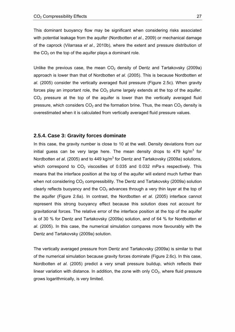
CO2 Compressibility Effects 27
This dominant buoyancy flow may be significant when considering risks associated
with potential leakage from the aquifer (Nordbotten et al., 2009) or mechanical damage
of the caprock (Vilarrasa et al., 2010b), where the extent and pressure distribution of
the CO2 on the top of the aquifer plays a dominant role.
Unlike the previous case, the mean CO2 density of Dentz and Tartakovsky (2009a)
approach is lower than that of Nordbotten et al. (2005). This is because Nordbotten et
al. (2005) consider the vertically averaged fluid pressure (Figure 2.5c). When gravity
forces play an important role, the CO2 plume largely extends at the top of the aquifer.
CO2 pressure at the top of the aquifer is lower than the vertically averaged fluid
pressure, which considers CO2 and the formation brine. Thus, the mean CO2 density is
overestimated when it is calculated from vertically averaged fluid pressure values.
2.5.4. Case 3: Gravity forces dominate In this case, the gravity number is close to 10 at the well. Density deviations from our
initial guess can be very large here. The mean density drops to 479 kg/m3 for
Nordbotten et al. (2005) and to 449 kg/m3 for Dentz and Tartakovsky (2009a) solutions,
which correspond to CO2 viscosities of 0.035 and 0.032 mPa·s respectively. This
means that the interface position at the top of the aquifer will extend much further than
when not considering CO2 compressibility. The Dentz and Tartakovsky (2009a) solution
clearly reflects buoyancy and the CO2 advances through a very thin layer at the top of
the aquifer (Figure 2.6a). In contrast, the Nordbotten et al. (2005) interface cannot
represent this strong buoyancy effect because this solution does not account for
gravitational forces. The relative error of the interface position at the top of the aquifer
is of 30 % for Dentz and Tartakovsky (2009a) solution, and of 64 % for Nordbotten et
al. (2005). In this case, the numerical simulation compares more favourably with the
Dentz and Tartakovsky (2009a) solution.
The vertically averaged pressure from Dentz and Tartakovsky (2009a) is similar to that
of the numerical simulation because gravity forces dominate (Figure 2.6c). In this case,
Nordbotten et al. (2005) predict a very small pressure buildup, which reflects their
linear variation with distance. In addition, the zone with only CO2, where fluid pressure
grows logarithmically, is very limited.
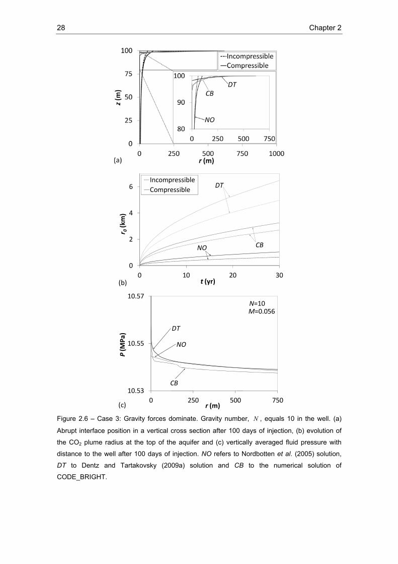
28 Chapter 2
0
2
4
6
0 10 20 30
r 0(km)
t (yr)
IncompressibleCompressible
DT
NO CB
(b)
10.53
10.55
10.57
0 250 500 750
P(M
Pa)
r (m)
DT
NO
CB
N=10
(c)
M=0.056
Figure 2.6 – Case 3: Gravity forces dominate. Gravity number, N , equals 10 in the well. (a)
Abrupt interface position in a vertical cross section after 100 days of injection, (b) evolution of
the CO2 plume radius at the top of the aquifer and (c) vertically averaged fluid pressure with
distance to the well after 100 days of injection. NO refers to Nordbotten et al. (2005) solution,
DT to Dentz and Tartakovsky (2009a) solution and CB to the numerical solution of
CODE_BRIGHT.
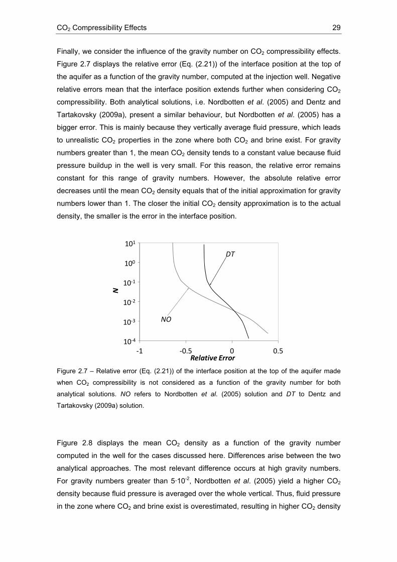
CO2 Compressibility Effects 29
Finally, we consider the influence of the gravity number on CO2 compressibility effects.
Figure 2.7 displays the relative error (Eq. (2.21)) of the interface position at the top of
the aquifer as a function of the gravity number, computed at the injection well. Negative
relative errors mean that the interface position extends further when considering CO2
compressibility. Both analytical solutions, i.e. Nordbotten et al. (2005) and Dentz and
Tartakovsky (2009a), present a similar behaviour, but Nordbotten et al. (2005) has a
bigger error. This is mainly because they vertically average fluid pressure, which leads
to unrealistic CO2 properties in the zone where both CO2 and brine exist. For gravity
numbers greater than 1, the mean CO2 density tends to a constant value because fluid
pressure buildup in the well is very small. For this reason, the relative error remains
constant for this range of gravity numbers. However, the absolute relative error
decreases until the mean CO2 density equals that of the initial approximation for gravity
numbers lower than 1. The closer the initial CO2 density approximation is to the actual
density, the smaller is the error in the interface position.
1.E‐04
1.E‐03
1.E‐02
1.E‐01
1.E+00
1.E+01
‐1 ‐0.5 0 0.5
N
Relative Error
NO
DT101
100
10‐1
10‐2
10‐3
10‐4
Figure 2.7 – Relative error (Eq. (2.21)) of the interface position at the top of the aquifer made
when CO2 compressibility is not considered as a function of the gravity number for both
analytical solutions. NO refers to Nordbotten et al. (2005) solution and DT to Dentz and
Tartakovsky (2009a) solution.
Figure 2.8 displays the mean CO2 density as a function of the gravity number
computed in the well for the cases discussed here. Differences arise between the two
analytical approaches. The most relevant difference occurs at high gravity numbers.
For gravity numbers greater than 5·10-2, Nordbotten et al. (2005) yield a higher CO2
density because fluid pressure is averaged over the whole vertical. Thus, fluid pressure
in the zone where CO2 and brine exist is overestimated, resulting in higher CO2 density

30 Chapter 2
values. For gravity numbers lower than 5·10-2, CO2 density given by Dentz and
Tartakovsky (2009a) is slightly higher than that of Nordbotten et al. (2005) because the
former predicts higher fluid pressure values in the CO2 rich zone, as explained
previously. However, both approaches present similar mean CO2 density values for low
gravity numbers.
1.E‐04
1.E‐03
1.E‐02
1.E‐01
1.E+00
1.E+01
400 650 900
N
Density (kg/m3)
DT
NO
101
100
10‐1
10‐2
10‐3
10‐4
Figure 2.8 – Mean CO2 density as a function of the gravity number in the cases discussed here
for both analytical solutions. NO refers to Nordbotten et al. (2005) solution and DT to Dentz and
Tartakovsky (2009a) solution.
2.6. Conclusions
CO2 compressibility effects may play an important role in determining the size and
geometry of the CO2 plume that will develop when supercritical CO2 is injected in an
aquifer. Here, we have studied the effect that accounting for CO2 compressibility
(density variations and corresponding changes in viscosity) exerts on the shape of the
plume computed by two abrupt interface analytical solutions. To this end, we have
presented a simple method to correct the initial estimation of the CO2 density and
viscosity and hence use more realistic values. These corrected values give a more
accurate prediction for the interface position of the CO2 plume.
The error associated with neglecting compressibility increases dramatically when
gravity forces dominate, which is likely to occur at late injection times. This is relevant
because the relative importance of buoyancy forces increases with distance to the
injection well. Thus gravity forces will ultimately dominate in most CO2 sequestration

CO2 Compressibility Effects 31
projects. As such incorporating CO2 compressibility is critical for determining the
interface position.
Comparison with numerical simulations suggests that the solution by Nordbotten et al.
(2005) gives good predictions when viscous forces dominate, while the Dentz and
Tartakovsky (2009a) solution provides good estimates of the CO2 plume position when
gravity forces dominate.

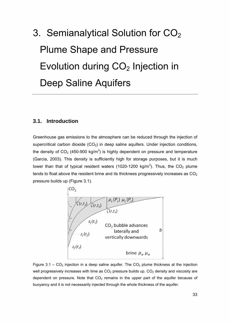
33
3. Semianalytical Solution for CO2
Plume Shape and Pressure
Evolution during CO2 Injection in
Deep Saline Aquifers
3.1. Introduction
Greenhouse gas emissions to the atmosphere can be reduced through the injection of
supercritical carbon dioxide (CO2) in deep saline aquifers. Under injection conditions,
the density of CO2 (450-900 kg/m3) is highly dependent on pressure and temperature
(Garcia, 2003). This density is sufficiently high for storage purposes, but it is much
lower than that of typical resident waters (1020-1200 kg/m3). Thus, the CO2 plume
tends to float above the resident brine and its thickness progressively increases as CO2
pressure builds up (Figure 3.1).
Figure 3.1 – CO2 injection in a deep saline aquifer. The CO2 plume thickness at the injection
well progressively increases with time as CO2 pressure builds up. CO2 density and viscosity are
dependent on pressure. Note that CO2 remains in the upper part of the aquifer because of
buoyancy and it is not necessarily injected through the whole thickness of the aquifer.

34 Chapter 3
Supercritical CO2 is very compressible and determining its density in the reservoir is
complicated because of the highly nonlinear and coupled relationships. On the one
hand, CO2 density depends on fluid pressure. On the other hand, fluid pressure buildup
during injection depends on CO2 density, because it determines the volume of
displaced brine. Pressure buildup is also controlled by other factors, like the the
caprock permeability (Birkholzer et al., 2009) or the nature of the aquifer boundaries
(Zhou et al., 2008). The resident brine can easily migrate out laterally in open aquifers.
This limits pressure buildup, but may salinize adjacent freshwater bodies. In contrast,
fluid and rock compressibility may limit storage capacity in the presence of low-
permeability boundaries (Zhou et al., 2008; Mathias et al., 2011). Estimating CO2
density is nontrivial because of the inherent nonlinearities and highly coupled nature of
this problem, as evidenced both in situ (Nooner et al., 2007) and analytically (Vilarrasa
et al., 2010a). Errors in CO2 density estimates will lead to errors in the CO2 plume
volume estimates. For instance, while 3D seismic data gave an average in situ CO2
density of 530 ± 65 kg/m3 at the Utsira formation (Sleipner, Norway), the CO2 density
estimates prior to the measurements ranged from 650 to 700 kg/m3 (Nooner et al.,
2007). CO2 density, which is a priori unknown, has to be chosen when using some
analytical solutions for determining the CO2 plume position. Neglecting CO2
compressibility can lead to errors greater than 50 % in the CO2 plume position at the
top of the aquifer (Vilarrasa et al., 2010a).
Existing analytical solutions also assume that the injection takes place uniformly along
the whole thickness of the aquifer (Saripalli and McGrail, 2002; Nordbotten et al., 2005;
Nordbotten and Celia, 2006; Dentz and Tartakovsky, 2009a; Manceau and Rohmer,
2011; Houseworth, 2012). This assumption is also unrealistic. Instead, one should
expect that most CO2 flows through the top portion of the aquifer, where the difference
between CO2 and resident water pressures are largest. In fact, the CO2 plume may
never reach the aquifer bottom (Figure 3.1). Even analytical solutions that predict the
CO2 plume evolution in the post-injection period consider that the CO2 plume occupies
the whole thickness of the aquifer at the end of the injection period (Hesse et al., 2007,
2008; Juanes et al., 2010). This may underestimate the CO2 volume in free-phase at
late times because the shape of the CO2 plume at the end of injection affects its post-
injection behaviour when capillary trapping is considered (MacMinn and Juanes, 2009).
In addition to the evolution of the CO2 plume, it is important to understand the evolution
of its pressure. Pressure affects the required compression energy, the CO2 density and
the mechanical stability of the caprock (Rutqvist et al., 2007; Ferronato et al., 2010;

Semianalytical Solution for Compressible CO2 Injection 35
Vilarrasa et al., 2010b). Mathias et al. (2009) assumed the Nordbotten et al. (2005)
solution for the CO2 plume position to calculate a vertical average of the fluid pressure
in the aquifer. The same result was obtained by Vilarrasa et al. (2010a), who extended
the computation to the solution of Dentz and Tartakovsky (2009a) and to calculate fluid
pressure at every point of the aquifer. However, fluid pressure obtained from these
analytical solutions differs significantly from that of numerical solutions (Vilarrasa et al.,
2010a).
This paper aims to develop a semianalytical solution that gives the CO2 plume position
and fluid pressure evolution accounting for CO2 compressibility and buoyancy effects in
the injection well. Thus, the extent and the thickness of the CO2 plume as well as the
overpressure can be quickly assessed. We formulate the problem and present the
methodology for solving it when the CO2 mass flow rate or the CO2 pressure are
prescribed at the injection well. Finally, we present an application of this methodology
and compare the results with full numerical simulations.
3.2. Problem formulation
Consider the injection of compressible CO2 through a vertical well in a deep
homogeneous horizontal confined brine aquifer. Mass conservation of these two fluids
can be expressed as (Bear, 1972)
( ) ( ) wctS , , =⋅−∇=∂
∂ αρϕραα
αα q , (3.1)
where αρ is fluid density of the α -phase, αS is the saturation of the α -phase, ϕ is
porosity, t is time and αq is the volumetric flux of the α -phase, which can be either c ,
the CO2 rich phase, or w , the aqueous phase.
Momentum conservation is expressed using Darcy’s law
( ) wczgPkkr , , =∇+∇−= αρμ ααα
ααq , (3.2)
where k is intrinsic permeability, αrk is relative permeability of the α -phase, αμ is
viscosity, αP is fluid pressure, g is gravity and z is the vertical coordinate (positive
upwards).
36 Chapter 3
This two-phase flow is affected by buoyancy effects because CO2 is lighter than brine.
To quantify the relative influence of buoyancy we define a gravity number, gN , as the
ratio of gravity to viscous forces. Gravity forces can be represented by the buoyancy
force ( gρΔ , where ρΔ is the difference between fluids density) in Darcy’s law,
expressed in terms of equivalent head. Viscous dissipation forces correspond to the
horizontal pressure gradient, which can be approximated as ( ( )απμ rrbkkQ 2/0 , where
0Q is the volumetric flow rate, r is radial distance and b is aquifer thickness).
However, since CO2 is compressible, it is more appropriate to express the volumetric
flow rate in terms of the mass flow rate, mQ , as ρmQQ =0 . Thus, gN becomes
,2mc
chrcchg Q
gbkkrNμ
ρρπ Δ= (3.3)
where chρ is a characteristic density and chr is a characteristic distance. Large values
of the gravity number ( 1>>gN ) indicate that buoyancy forces dominate. On the other
hand, small gravity numbers ( 1<<gN ) indicate that viscous forces dominate. Notice
that buoyancy forces will always dominate far from the injection well, where chr is
sufficiently large, whereas the opposite will be true near the well.
Assuming that fluid density depends only on fluid pressure, the head of the α -phase is
defined as (Bear, 1972)
( )∫ ′′
+−=α
αα
αα ρ
P
P PP
gzzh
0
d10 , (3.4)
where αh is head of the α -phase, 0z is a reference depth and 0P is the hydrostatic
fluid pressure corresponding to depth 0z .
Darcy’s law can be expressed in terms of head provided that density is not affected by
other variables (i.e. under isothermal conditions) by combining Eq. (3.2) and (3.4)
ααα
αα ρ
μhgkkr ∇−=q . (3.5)
When flow rate is prescribed at the injection well, CO2 will penetrate initially along the
top portion of the aquifer because its pressure is not sufficient to displace brine along
the entire aquifer thickness. The CO2 plume advances both laterally and vertically
downwards as pressure builds up. CO2 occupies the portion of the well where CO2

Semianalytical Solution for Compressible CO2 Injection 37
pressure is higher than brine pressure (Figure 3.1). Brine and CO2 pressures are
related at the porous medium interface via the capillary entry pressure
cciwic PzrPzrP += ),(),( , (3.6)
where ccP is the capillary entry pressure and ir is the radial position of the interface at
depth z .
Neglecting mass transfer across the interface, the problem is defined by the two
differential equations in (3.1), one for each phase, which are coupled by the equilibrium
equation in (3.6) and by the continuity of flux at the interface
( )zrzr iwic ,),( qq = . (3.7)
The boundary condition at the injection well is a prescribed CO2 mass flow rate or CO2
pressure. As for the outer boundary, we consider an infinite aquifer.
3.3. Semianalytical solution
3.3.1. Radial injection of compressible CO2 To address the problem of CO2 injection defined in the previous section we assume
that the CO2 rich phase and the formation brine are separated by a sharp interface.
This assumption is reasonable from an analytical perspective in the context of CO2
sequestration (Nordbotten et al., 2005; Dentz and Tartakovsky, 2009a, 2009b; Lu et al.,
2009). Capillary pressure is considered at the interface between the CO2 rich phase
and the formation brine (Eq. (3.6)). Thus, there is a jump in fluid pressure at the
interface equal to the entry pressure. CO2 dissolution into the brine, which may induce
density-driven convective cells (Lindeberg and Wessel-Berg, 1997; Riaz et al., 2006;
Hidalgo and Carrera, 2009; Pau et al., 2010), is not considered.
We solve the problem by vertically discretizing the aquifer into n layers of thickness
nbd = (Figure 3.2). The time evolution of the problem is solved using discrete time
steps to overcome nonlinearities and coupling difficulties. The interface advances
laterally in the layers that contain CO2, but also moves vertically downwards as fluid
pressure builds up. CO2 at the bottom of the CO2 plume may fill the thickness of a layer
only partially. Once the CO2 plume reaches a thickness equal to md , where m is the
number of layers filled with CO2, the following layer 1+m , previously devoid of CO2,

38 Chapter 3
begins to fill up with CO2. The part occupied by CO2 in this new layer has a thickness
equal to mdbc − , where cb is the CO2 plume thickness at the well (Figure 3.2).
Figure 3.2 – Schematic representation of CO2 injection evolution taking into account that CO2
first enters through the top of the aquifer because of buoyancy. The aquifer is divided into n
layers through which CO2 advances laterally and vertically downwards. The CO2 plume
reaches, at every time step, the depth at which CO2 pressure equals brine pressure plus the
capillary entry pressure.
To calculate the CO2 plume thickness in the injection well, we assume hydrostatic
conditions in it,
( ) wcPgzP , ,d
d=−= αρ αα
α . (3.8)
To calculate the lateral advance of CO2 in each layer, we assume that the hydraulic
response within the CO2 plume is much shorter than transport of the front. Therefore,
we consider a quasi-steady (sequence of steady-states) description of the moving
fronts in Eq. (3.1). Hence, the left-hand side of Eq. (3.1) cancels. Additionally, we make
the Dupuit approximation of horizontal flow. Furthermore, the density of the CO2 phase
will vary in space because so will the CO2 pressure and because of the high
compressibility of CO2. Therefore, conservation should not be expressed in terms of
volumetric fluxes, but mass fluxes. The total mass flow rate, per unit aquifer thickness,
in a radial injection varies with depth but is constant at a given z within each phase
ααα ρπ rqrJ 2= , (3.9)

Semianalytical Solution for Compressible CO2 Injection 39
where αJ is the mass flow rate per unit thickness of α -phase and αrq is the horizontal
component of the volumetric flux of α -phase. This mass flow rate per unit thickness
will vary from layer to layer. At the interface in each layer, we impose continuity of flux
in the radial direction
( )zrqzrq jrwjrc ,),( = , (3.10)
where jr is the radius of the interface in layer j .
Since we adopt a sharp interface approximation, the saturation in the CO2 rich phase is
taken as constant. Thus, the interface position advances as
( )( )rw
jrj
Srq
dtdr
−=
1ϕα , (3.11)
where rwS is the residual degree of saturation of brine.
To eliminate the complexities associated to nonlinearity, we define the following
potential to formulate the problem assuming that relative permeability and fluid density
are solely a function of fluid pressure
( ) ( )( )∫ ′
′′=Φ
α
αα
αααααα μ
ρπh
r hhhgkkh0
2*
d2)( , (3.12)
where ( ) ( )( )ααααα ρρ hPh ′=′ ** .
Combining Eq. (3.5), (3.9) and (3.12), flow rate in the layer becomes
αα Jr
r −=Φd
d. (3.13)
Though we make the Dupuit approximation of horizontal flow within a layer, we
acknowledge the vertical CO2 leakage between layers. Acknowledging that flow
towards the aquifer top is largely buoyancy driven, we impose that the vertical mass
flow rates between layers occur punctually, for simplicity. The distance at which the
vertical flow rates are injected to the adjacent layer depends on the gravity number
computed in the vicinity of the injection well (Eq. (3.3)). This is because vertical flow
rates are expected to occur when gravity forces dominate, i.e. large gravity numbers.
Then, vertical flow rates will occur close to the injection well for large gravity numbers.
On the other hand, vertical flow rates will occur far from the injection well for small
gravity numbers computed close to the injection well. Therefore, the distance at which
40 Chapter 3
the vertical flow rates occur is inversely proportional to the gravity number. The vertical
mass flow rate of a layer to its adjacent one is given by
∫=j
p
r
rzccjcz rqJ d2, πρ , (3.14)
where pr is the radius of the well and zcq is the vertical component of the volumetric
CO2 flux. We will inject this flow rate at a radius ( ))2(,min 1 gjj Nbrr += . The term
)2( gNb is somewhat arbitrary, and can be chosen case specifically. For simplicity, we
have adopted 1+jr as jr . Introducing Eq. (3.5) into Eq. (3.14) and assuming that the
CO2 head varies linearly with the logarithm of distance to the well, after some algebra,
yields
( ) ⎟⎟⎠
⎞⎜⎜⎝
⎛−−−
Δ= +
+++p
jjpjjj
jc
crcjcz r
rrrruu
zgkkJ 1
111
2
, ln2μ
ρπ, (3.15)
where ju is the logarithmic slope of the CO2 head in layer j , jzΔ is the thickness of
the layer j and CO2 density is evaluated at the point of the vertical flow rate injection.
Note that the subscript of the layers increases with depth, i.e. layer j is placed above
layer 1+j .
The integration of Eq. (3.13), accounting for the fact that now cJ is a function of the
radial distance due to the vertical flow rates, yields the solution of the problem
jjwRjw rrrRJ ≥⎟⎠⎞
⎜⎝⎛+Φ=Φ ,ln,, (3.16a)
( ) jjj
jczjcjjc rrrrr
JJ <<⎟⎟⎠
⎞⎜⎜⎝
⎛++Φ=Φ ++ 11,,, ,ln (3.16b)
11
1,,, ,lnln ++
+ <⎟⎟⎠
⎞⎜⎜⎝
⎛+⎟⎟
⎠
⎞⎜⎜⎝
⎛+Φ=Φ j
j
jjcz
jjcjjc rr
rr
Jrr
J (3.16c)
where RΦ is the potential at the radius of influence, R is the radius of influence, the
subscript after the comma indicates the layer (e.g. j, indicates layer j ) and jΦ is the
potential at the interface in layer j . RΦ is known and constant because it refers to the
initial fluid pressure in the aquifer. jΦ can be determined by evaluating Eq. (3.16a) at
the interface. The radius of influence corresponds to the distance affected by the
pressure buildup cone caused by injection and grows with the square root of time as
Semianalytical Solution for Compressible CO2 Injection 41
sw
w
SgtkR
μρ25.2
= , (3.17)
where sS is the specific storage coefficient.
The CO2 mass flow rate at the injection well for layer j can be determined from Eq.
(3.16c) as
( ) ( )( )pj
jjjczjpjcjc rr
rrJrJ
lnln 11,,
,++−Φ−Φ
= . (3.18)
This CO2 mass flow rate will change with time as the CO2 plume grows. The evolution
of the CO2 plume is calculated using a time stepping algorithm. Integrating Eq. (3.11)
and using Eq. (3.9) yields the interface position for a given time step
( ) ( ) ljcirw
lj
ljcl
jlj S
trJrzr
,
1,21
1)(
)(ρπϕ −
Δ+=
++ , (3.19)
where the superscript l denotes the time step, tΔ is increment of time between step l
and step 1+l and jci ,ρ is the CO2 density at the interface in layer j .
The volumetric flow rate of brine, wQ , at a radial distance r from the well can be
calculated once the interface position is known. Due to the continuity of fluxes at the
interface, we obtain
( ) ( )( )
( )
∫−
=rz
z c
cw
f
zrrJrQ
ζ
ρ
0
d , (3.20)
where fz is the depth of the bottom of the CO2 plume and ζ is the vertical position of
the CO2 plume from the top of the aquifer.
The volume of displaced brine at radius r is equal to the volume of injected CO2. The
flow rate of brine is driven by the overpressure produced by the injected CO2, which is
assumed to be distributed through the portion of the aquifer thickness occupied by the
formation brine
( ) zrPkrrQ w
w
rz
bzw d2
)(0
0∂∂
−= ∫−
− μπ
ζ
. (3.21)
Integrating Eq. (3.21) yields the following expression for brine pressure
42 Chapter 3
( )( )( ) r
RrbkrQPP ww
w ln20 ζπμ
−=− . (3.22)
The problem accepts two possible boundary conditions at the injection well. Either a
prescribed CO2 mass flow rate or a prescribed CO2 pressure can be imposed.
3.3.2. Prescribed CO2 mass flow rate When injecting a prescribed CO2 mass flow rate, the CO2 plume advances both
laterally and vertically downwards as CO2 pressure builds up. Since this problem
presents two unknowns at every time step, i.e. the CO2 head at the well and the
thickness of the CO2 plume at the well, two conditions are needed. First, hydrostatic
conditions are assumed in the well (Eq. (3.8)) accounting for the capillary entry
pressure at the CO2-brine interface (Eq. (3.6)). And second, mass balance must be
satisfied. The mass inlet at a given time step corresponds to the mass flow rate
multiplied by the time increment. This mass is distributed through the layers containing
CO2 proportionally to the mass flow rate per unit thickness and the thickness of each
layer. Furthermore, the mass that occupies the volume corresponding to the increment
of the plume thickness in each time step has to be accounted for, resulting in
( )tz
SrzJQ frwifcj
m
jjcm Δ
Δ−+Δ=∑
=
12
1, ϕπρ , (3.23)
where mQ is the prescribed CO2 mass flow rate, m is the total number of layers in
which CO2 is present, cρ is the mean CO2 density in the layer that coincides with the
bottom of the CO2 plume, ifr is the interface position at the bottom of the CO2 plume
and fzΔ is the increment of the CO2 plume thickness at the well at a given time step.
3.3.3. Prescribed CO2 pressure Since the head at the well is known when imposing the CO2 pressure, there is only one
unknown: the thickness of the CO2 plume at the well. Hence, imposing hydrostatic
conditions in the well (Eq. (3.8)) and that the thickness of the CO2 plume in the well is
such that the CO2 pressure equals the brine pressure plus the capillary entry pressure
(Eq. (3.6)) allows solving the problem.
Semianalytical Solution for Compressible CO2 Injection 43
3.4. Algorithm
The evolution of the position of the CO2 plume is calculated using a time stepping
algorithm. The process is very similar for the two possible injection boundary conditions
and is repeated for each time step (Figure 3.3). The procedure has to be initialized,
using a small time increment, as follows
• The CO2 plume is assumed to grow slightly in the top layer, i.e. the interface
position advances laterally a fraction of the well radius and the thickness of the
CO2 plume is a fraction of d .
• The volumetric flow rate is assumed equal to the mass flow rate divided by
density at the reference CO2 pressure.
These two assumptions allow initializing the overpressure (using Eq. (3.22) and the
volumetric flow rate), the potential at the interface (using Eq. (3.12)), the depth that
reaches the CO2 plume, the head at the injection well and the potential at the well
(using Eq. (3.12)). No vertical flow rates exist in this initialization. The time stepping
algorithm can then be used after obtaining these data. It is as follows
1) Determine the vertical CO2 mass flow rate (Eq. (3.15)) and the horizontal
CO2 mass flow rate in each layer evaluating Eq. (3.18) at the well. We use
the potential at the interface and at the well and the interface position
evaluated at the previous time step.
2) Calculate the new interface position in every layer using Eq. (3.19). The CO2
mass flow rate is the one calculated in step 1 and the CO2 density at the
interface is the one evaluated at the previous time step.
3) Calculate the potential at the interface (Eq. (3.12)), using Eq. (3.20) to
calculate the volumetric flow rate and Eq. (3.22) to calculate the brine
pressure, and Eq. (3.6) to calculate the CO2 pressure at the interface.
4.1) Impose a prescribed CO2 mass flow rate: solve the system of two equations
(Eqs. (3.23) and (3.8) accounting for the capillary entry pressure in (3.6)) and
determine the CO2 head at the well and the thickness of the CO2 plume at
the well.
4.2) Impose a prescribed CO2 pressure: the head at the well can be determined
by using Eq. (3.4) and the thickness of the CO2 plume at the well can be
calculated by imposing Eq. (3.8) accounting for the capillary entry pressure in
(3.6).

44 Chapter 3
5) Based on the head at the well calculated in step 4, compute the potential at
the well using Eq. (3.12).
These five steps are repeated, applying a time increment after every loop, until CO2
injection is completed.
Figure 3.3 – Time stepping algorithm to calculate the position of the CO2 plume and the fluid
pressure.
3.5. Application
3.5.1. Spreadsheet programming In order to evaluate this methodology, we programmed it in a spreadsheet that can be
downloaded from GHS (2012). We programmed it this way to highlight ease of
implementation and use by non-expert programmers. This spreadsheet considers 25
layers, a prescribed mass flow rate, constant properties of the brine (density and
viscosity), constant CO2 viscosity and the CO2 density is defined to vary linearly with
CO2 pressure
Semianalytical Solution for Compressible CO2 Injection 45
( )00 PPcc −+= βρρ , (3.24)
where 0ρ is the reference density for the reference pressure 0P and β is CO2
compressibility. These values were taken from the data tables given by Span and
Wagner (1996).
With this linear approximation of the CO2 density, the potential for the CO2 can be
obtained by integrating Eq. (3.12), which yields (see Appendix III)
( )( )12220 0 −=Φ −− chgzzg
cc eek ββ
βμρπ
. (3.25)
Furthermore, CO2 pressure can be expressed as a function of the potential (Appendix
III)
( )
βρ
βρ
βπμ β 02
2
20
00 −+Φ=− −− zzg
cc
c ek
PP . (3.26)
Note that CO2 overpressure varies with the square root of the logarithm of the distance
to the injection well (see the form of the potential cΦ in Eq. (3.16b,c)).
The solution of the system of two equations (Eqs. (3.8) and (3.23)) for finding the CO2
head and the thickness of the CO2 plume at the well is shown in Appendix IV. The
mean density appearing in Eq. (3.23) is calculated in Appendix V.
3.5.2. Model setup We represent a 100 m thick saline aquifer whose top is located at a depth of 1000 m.
The aquifer is assumed to be infinite-acting, homogeneous and isotropic. The
permeability of the aquifer is either 10-12 or 10-13 m2, its porosity is 0.1 and the rock
compressibility is 1.2·10-10 Pa-1. The temperature is assumed to be constant and equal
to 320 K. The density of brine is 1087.5 kg/m3, its viscosity is 0.6 mPa·s and its
compressibility is 4.5·10-10 Pa-1. Thus, the specific storage coefficient yields a value of
1.76·10-6 m-1. The reference CO2 density 0ρ , corresponding to the reference pressure
0P =10 MPa (hydrostatic pressure at the top of the aquifer), is 448.28 kg/m3 and its
compressibility β is 5.56·10-5 kg/m3·Pa-1 (Span and Wagner, 1996). β is the product
of the actual CO2 compressibility and a density. The actual CO2 compressibility at the
pressure and temperature of the aquifer is 1.48·10-7 Pa-1. Note that CO2
compressibility, for the range of pressure and temperature of this study, is three orders
46 Chapter 3
of magnitude higher than that of brine. The CO2 viscosity is calculated using the
expression proposed by Altunin and Sakhabetdinov (1972). Though constant, CO2
viscosity is case specific and depends on the overpressure, so that a representative
value can be adopted according to the mean CO2 density. The entry pressure equals
0.02 MPa and the residual degree of saturation of brine is 0.025. The injected mass
flow rate is 1.0 Mt/yr. An injection ramp is used to progressively increase the mass flow
rate from zero to the desired mass flow rate. Doing so, the increments in the CO2
plume thickness are small. This injection ramp lasts less than 50 s, so its effect can be
considered as negligible for practical purposes.
The finite element numerical code CODE_BRIGHT (Olivella et al., 1994; 1996),
extended for CO2 sequestration (Appendix II), has been used to validate the results of
this semianalytical solution with those of numerical results. The aquifer is represented
by an axisymmetric model, with a radius of 100 km, in which CO2 is injected at the top
of the injection well. The radius of the injection well is 0.5 m. The well is modelled
assigning a porosity equal to 1 and a high permeability. The grid is structured and has
25 elements in the vertical coordinate in order to represent the 25 layers adopted in the
application of the semianalytical solution. We used a van Genuchten retention curve
(van Genuchten, 1980), with an entry pressure of 0.02 MPa and a shape parameter of
0.8. The relative permeability functions, for both the CO2 and the brine, are linear with
the degree of saturation of each phase. These retention curve and relative permeability
functions produce a CO2 plume with an almost constant CO2 saturation and a narrow
capillary fringe. Thus, the numerical solutions are close to the assumption of the abrupt
interface approximation assumed for the semianalytical solution. The CO2 saturation 90
% isoline has been chosen to represent the position of the CO2-brine interface.
3.5.3. Validation of the semianalytical solution We compare the results of the semianalytical solution with those of the numerical
solution. Additionally, the analytical solutions of Nordbotten et al. (2005) and Dentz and
Tartakovsky (2009a) using the method proposed by Vilarrasa et al. (2010a) to account
for CO2 compressibility are presented for comparative purposes. These analytical
solutions inject CO2 uniformly in the whole thickness of the aquifer, which may not be
realistic.
Figure 3.4 displays the CO2 plume position for the analytical, semianalytical and
numerical solutions after 1 yr of injecting 1 Mt/yr of CO2 for two aquifer permeabilities.

Semianalytical Solution for Compressible CO2 Injection 47
We consider a case with high permeability ( k =10-12 m2) in which gravity forces
dominate and another case with low permeability ( k =10-13 m2) in which viscous forces
dominate. The semianalytical solution compares well with the numerical solution in
both cases. The CO2 plume occupies only the top portion of the aquifer when gravity
forces dominate (CO2 is injected into the aquifer through the top 32 m) (Figure 3.4a).
On the other hand, the CO2 plume reaches the bottom of the aquifer when viscous
forces dominate (Figure 3.4b). The Nordbotten et al. (2005) solution gives a better
approximation when viscous forces dominate, while the Dentz and Tartakovsky
(2009a) solution predicts a better CO2 plume position when gravity forces dominate.
However, both analytical solutions differ from the numerical solution at the bottom of
the CO2 plume due to the fact that they consider a uniform injection along the whole
thickness of the aquifer.
Figure 3.5 compares fluid overpressure at the top of the aquifer as a function of the
distance to the injection well resulting from the semianalytical, numerical and analytical
solutions when injecting 1.0 Mt/yr in an aquifer with a permeability of 10-13 m2. Fluid
overpressure obtained from the semianalytical solution compares well with that of the
numerical solution, presenting the same slope in the region occupied by CO2 close to
the injection well. The pressure drop increases sharply at the distance where CO2 from
the second layer is injected in the top layer. This is in contrast with the numerical
solution, where the gradient increases smoothly. As a result, our solution is somewhat
more abrupt than the numerical solution near the interface. Existing analytical
solutions, i.e. those of Nordbotten et al. (2005) and Dentz and Tartakovsky (2009a), fail
to give good fluid pressure predictions. First, they predict a lower brine overpressure
because they underestimate the volumetric flow rate of brine. This is because CO2 is
injected along the whole thickness of the aquifer and since CO2 density increases with
depth, the mean CO2 density becomes higher than in the semianalytical and numerical
solutions. Additionally, the slopes of fluid pressure inside the CO2 plume are lower than
that of numerical simulations. In contrast, the slope of the semianalytical solution is the
same as that of the numerical solution close to the injection well in the region occupied
by CO2. Hence, it can be concluded from this semianalytical solution that while brine
overpressure is proportional to the logarithm of distance from the injection well, CO2
overpressure is proportional to the square root of the logarithm of the distance from the
injection well (recall Eq. (3.26)).

48 Chapter 3
1000
1020
1040
1060
1080
11000 500 1000 1500
z(m
)
r (m)
NSSSNDT
Qm=1.0 Mt/yrk=10‐12 m2
t=1 yrNg=1.55
(a)
1000
1020
1040
1060
1080
11000 500 1000
z(m
)
r (m)
NSSSNDT
Qm=1.0 Mt/yrk=10‐13 m2
t=1 yr
(b)
Ng=0.15
Figure 3.4 – Comparison of the CO2 plume position between semianalytical (SS) and numerical
solution (NS) after 1 yr of injection of 1 Mt/yr, and permeabilities, k , (a) k =10-12 m2 and (b)
k =10-13 m2. Additionally, the analytical solutions of Nordbotten et al. (2005) (N) and Dentz and
Tartakovsky (2009a) (DT) after using the method of Vilarrasa et al. (2010a) to account for CO2
compressibility are presented for comparison. Note that these analytical solutions inject CO2
uniformly along the whole thickness of the aquifer.
Figure 3.6 displays the evolution of the overpressure at the injection well when injecting
1.0 Mt/yr in an aquifer with a permeability of 10-13 m2. While the overpressure predicted
by the analytical solutions of Nordbotten et al. (2005) and Dentz and Tartakovsky
(2009a) increases continuously, fluid overpressure decreases after reaching a
maximum at the beginning of injection for the semianalytical and numerical solutions.
Mukhopadhyay et al. (2012) found that overpressure increases continuously when
injecting CO2 in depleted gas reservoirs, whose fluid pressure is significantly below
hydrostatic conditions. However, a pressure drop after the initial pressure build up was
observed in situ in the Ketsin test site, Germany (Henninges et al., 2011) and

Semianalytical Solution for Compressible CO2 Injection 49
numerically by Vilarrasa et al. (2010b), who argued that pressure drops because the
overpressure that occurs in the capillary fringe due to relative permeability reduction is
distributed over a larger area as the CO2 plume increases and because the viscosity of
the CO2 is much lower than that of the brine.
0.8
1.2
1.6
2.0ΔP
(MPa)
r (m)
NSSSNDT
100 101 102 103 104
Figure 3.5 – Comparison of the fluid overpressure at the top of the aquifer between analytical,
semianalytical (SS) and numerical solutions (NS) after 1 yr injecting 1.0 Mt/yr in an aquifer with
a permeability of 10-13 m2. The analytical solutions of Nordbotten et al. (2005) (N) and Dentz and
Tartakovsky (2009a) (DT) after using the method of Vilarrasa et al. (2010a) to account for CO2
compressibility are presented for comparison. The first change in slope beginning from the right
hand side of the figure indicates the CO2-brine interface position for each solution.
1.6
1.8
2.0
2.2
2.4
0.0 0.2 0.4 0.6 0.8 1.0
ΔP (M
Pa)
t (yr)
NSSSNDT
Figure 3.6 – Comparison of the time evolution of the injection pressure at the top of the aquifer
between analytical, semianalytical (SS) and numerical solutions (NS) when injecting 1.0 Mt/yr in
an aquifer with a permeability of 10-13 m2. The analytical solutions of Nordbotten et al. (2005) (N)
and Dentz and Tartakovsky (2009a) (DT) after using the method of Vilarrasa et al. (2010a) to
account for CO2 compressibility are presented for comparison.

50 Chapter 3
3.5.4. CO2 plume thickness Figure 3.7 shows the CO2 plume position evolution for several injection times given by
the semianalytical solution when injecting 1.0 Mt/yr in an aquifer with a permeability of
10-13 m2. CO2 advances laterally and vertically downwards as pressure builds up. Note
that the CO2 plume advances preferentially through the top of the aquifer for increasing
injection times. This is because gravity forces become dominant as CO2 flows away
from the injection well. Note that in this case the CO2 plume reaches the aquifer bottom
for an injection time longer than 30 days (actually, it occurs after 162.6 days of
injection). However, the CO2 plume would not reach the bottom of the aquifer in a more
permeable aquifer, like the one presented in Figure 3.4a.
1000
1020
1040
1060
1080
1100
z(m
)
r (m)100 101 102 103 104
t=0.02 d t=1 d t=30 d t=5 yr
Qm=1.0 Mt/yrk=10‐13 m2
Figure 3.7 – CO2 plume evolution given by the semianalytical solution for several injection times
when injecting 1.0 Mt/yr in a 100 m thick aquifer with a permeability of 10-13 m2. Note that the
thickness of the CO2 plume progressively increases with injection time.
Figure 3.8 displays the CO2 plume thickness at the well after 1 yr of injection as a
function of the gravity number computed at 1 m from the injection well (Eq (3.3)) for
several aquifer permeabilities. The curves are obtained by varying the mass flow rate.
The logarithm of the CO2 plume thickness decreases linearly with the logarithm of the
gravity number, presenting a slope of -0.5. The CO2 plume is thinner than the aquifer
thickness for high gravity numbers (buoyancy forces dominate). In contrast, it reaches
the bottom of the aquifer for gravity numbers lower than 0.15 (viscous forces
dominate). The effect of the permeability is small, but not negligible because
permeability affects fluid overpressure and thus CO2 density. These curves are useful
for quickly estimating the CO2 thickness at the well of a CO2 injection project.
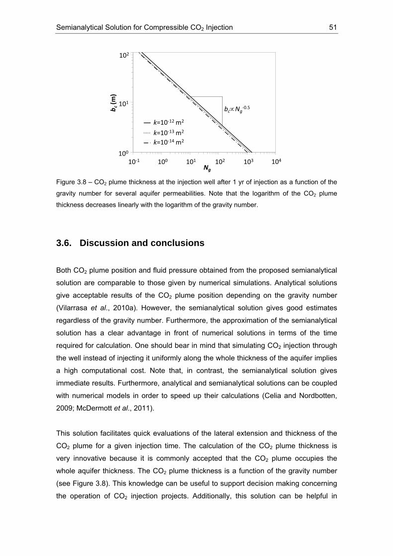
Semianalytical Solution for Compressible CO2 Injection 51
b c(m
)
Ng
Series1Series2Series3
k=10‐12 m2
k=10‐13 m2
k=10‐14 m2
bc∝Ng‐0.5
100
101
102
10‐1 100 101 102 103 104
Figure 3.8 – CO2 plume thickness at the injection well after 1 yr of injection as a function of the
gravity number for several aquifer permeabilities. Note that the logarithm of the CO2 plume
thickness decreases linearly with the logarithm of the gravity number.
3.6. Discussion and conclusions
Both CO2 plume position and fluid pressure obtained from the proposed semianalytical
solution are comparable to those given by numerical simulations. Analytical solutions
give acceptable results of the CO2 plume position depending on the gravity number
(Vilarrasa et al., 2010a). However, the semianalytical solution gives good estimates
regardless of the gravity number. Furthermore, the approximation of the semianalytical
solution has a clear advantage in front of numerical solutions in terms of the time
required for calculation. One should bear in mind that simulating CO2 injection through
the well instead of injecting it uniformly along the whole thickness of the aquifer implies
a high computational cost. Note that, in contrast, the semianalytical solution gives
immediate results. Furthermore, analytical and semianalytical solutions can be coupled
with numerical models in order to speed up their calculations (Celia and Nordbotten,
2009; McDermott et al., 2011).
This solution facilitates quick evaluations of the lateral extension and thickness of the
CO2 plume for a given injection time. The calculation of the CO2 plume thickness is
very innovative because it is commonly accepted that the CO2 plume occupies the
whole aquifer thickness. The CO2 plume thickness is a function of the gravity number
(see Figure 3.8). This knowledge can be useful to support decision making concerning
the operation of CO2 injection projects. Additionally, this solution can be helpful in
52 Chapter 3
designing and interpreting CO2 injection tests in pilot projects. In this context, it is
important to bear in mind that, from a storage point of view, it is desirable to inject over
the whole aquifer thickness to maximize the use of pore space. As we have seen, this
goal is limited by buoyancy, which dominates far from the injection well. Still, even near
the well, injecting over a partial thickness may be profitable during early stages
because it promotes CO2 dissolution into the brine, which in turn may cause CO2
dissolution and stimulation quite far from the injection well. For such goal, our solution,
generalized for varying permeability, would be extremely useful.
Finally, the slope of CO2 pressure as a function of the logarithm of distance from the
well calculated with the semianalytical solution is the same as that of the numerical
solution. In the semianalytical solution, the CO2 overpressure varies with the square
root of the logarithm of the distance to the injection well (Eq. (3.26)). This is interesting
because this variation with distance to the well differs from those of existing analytical
solutions. Additionally, the semianalytical solution reproduces a CO2 injection pressure
evolution similar to the one observed in numerical solutions and at the field, i.e. fluid
pressure drops after an initial abrupt fluid pressure buildup. This behaviour, which
appears naturally in this semianalytical solution, is not reflected by other existing
analytical solutions.

53
4. Coupled Hydromechanical
Modeling of CO2 Sequestration in
Deep Saline Aquifers
4.1. Introduction
Carbon dioxide (CO2) sequestration in deep saline aquifers is considered a promising
mitigation option for the reduction of CO2 emissions to the atmosphere. Injecting CO2
into aquifers at depths greater than 800 m brings CO2 to a supercritical state where its
density is large enough to ensure an efficient use of pore space (Hitchon et al., 1999).
Although the density of CO2 can reach values as high as 900 kg/m3, it will always be
lighter than the resident brine. Consequently, it will flow along the top of the aquifer
because of buoyancy. Thus, suitable aquifers should be capped by a low-permeability
rock to avoid CO2 migration to upper aquifers and the surface. Caprock discontinuities,
such as fractured zones, may favor upwards CO2 migration. Additionally, CO2 injection
can result in significant pressure buildup, which affects the stress field and may induce
large deformations. These can eventually damage the caprock and open up new flow
paths. These interactions between fluid flow and rock mechanics are known as
hydromechanical coupling.
Hydromechanical (HM) processes generally play an important role in geological media,
and in particular during CO2 injection into deep saline aquifers. These formations are
usually fluid-saturated fractured rock masses. Therefore, they can deform either as a
result of changes in external loads or internal pore pressures. This can be explained
with direct and indirect HM coupling mechanisms (Rutqvist and Stephansson, 2003).
Direct HM coupling consists of two phenomena: a solid-to-fluid coupling in which a
variation in the applied load induces a change in porosity and thus in fluid pressure or
mass; and a fluid-to-solid coupling that takes place when a change in fluid pressure or
fluid mass causes a variation in the volume of the geological media. On the other hand,
54 Chapter 4
indirect HM coupling refers to changes in hydraulic or mechanical properties in
response to strain.
In practice, using HM couplings allows us to determine conditions under which
mechanical failure (shear failure or hydraulic fracture) could occur so that injection
pressures can be limited below a fracturing threshold. Rutqvist et al. (2008) found that
shear failure usually occurs at a lower injection pressure than hydro fracturing. When
horizontal stress is greater than vertical stress ( vh σσ > ), shear failure will occur
preferentially in gently dipping fractures, without damage to the upper part of the
caprock. However, when vertical stress is greater than horizontal stress ( vh σσ < ) the
propagation of fractures is most likely to occur in the form of steeply dipping fractures
which could penetrate the entire caprock.
Existing simplified analytical solutions for determining the maximum sustainable
pressure often predict incorrect values (Rutqvist et al., 2007, Vidal-Gilbert et al., 2008),
suggesting that the fully coupled problem should be solved. Nonetheless, the majority
of CO2 injection simulations only model the multiphase flow problem (e.g. Doughty and
Pruess, 2004; Ide et al., 2007), without mechanical coupling. Some of these numerical
studies reproduce pilot CO2 injection tests (Doughty et al., 2006; Ghomian et al., 2008).
Given that small quantities of CO2 are usually injected in pilot tests, rock stability is not
a concern. The computational burden is much higher using the hydromechanical
coupling than the hydraulic problem (Tran et al., 2004). Nevertheless, coupling
strategies are available to avoid the full coupling (i.e. solving the flow and mechanical
problem together), such as explicit or iterative coupling or, even, decoupling. These
schemes allow reducing the computational burden, but at the expense of some loss of
accuracy (Mainguy and Longuemare, 2002; Settari and Walters, 1999).
The vast majority of rocks present very small yield stresses (Cristescu, 1989). As
pressure buildup caused by CO2 injection will affect a large extension of the aquifer and
caprock over several decades, irreversible strains are expected to occur. However,
poroelasticity is usually adopted to resolve the mechanical problem (Rutqvist et al.,
2008, Vidal-Gilbert et al., 2008). Although this approach gives a good approximation,
an elasto-plastic constitutive model provides more precise results (Settari and Walters,
1999).
Strains are induced by fluid pressure evolution, which depends on the hydraulic

Coupled Hydromechanical Modeling of CO2 Sequestration 55
boundary conditions. Aquifers are sometimes assumed to be infinite (Rutqvist et al.,
2008; van der Meer and van Wees, 2006). In modeling practice, this means that the
boundary is placed far enough to ensure that it does not affect fluid flow. In fact, deep
saline aquifers for CO2 sequestration may extend tens or even hundreds of kilometers
(McPherson and Cole, 2000; Zhang et al., 2009). However, CO2 sequestration projects
will span several decades. Therefore, the radius of influence ( )/(25.2 sww SgtkR μρ= ,
where k is the intrinsic permeability, wρ is water density, g is gravity, t is time, wμ is
water viscosity and sS is the specific storage coefficient of the aquifer) propagates over
large distances, reaching the boundaries much earlier than the end of operations
(Birkholzer et al., 2009). In such cases, the infinite acting aquifer assumption may not
be appropriate and the nature of the boundary may have to be addressed. Aquifers can
be classified as open and semi-closed, depending on the nature of the boundaries.
Open aquifers can be modeled with a constant head boundary condition (Lucier and
Zoback, 2008), and semi-closed aquifers with a leakage coefficient. In open aquifers
brine could escape and salinize fresh water bodies (Birkholzer and Zhou, 2009). In
closed and semi-closed aquifers, the CO2 storage capacity is basically controlled by
rock and fluid compressibility (Vilarrasa et al., 2010a; Zhou et al., 2008). Given that a
low-permeability boundary can be modeled with a leakage coefficient, the role of such
a boundary condition should be evaluated. The effect that a low-permeability boundary
has on fluid flow has been studied in hydrogeology (e.g. Wheatcraft and Winterberg,
1985; Butler, 1988). Although these studies deal with single phase flows, they can be
helpful and valid in two phase flows (e.g. Neuweiler et al., 2003; Bolster et al., 2009b).
The other boundary condition that affects fluid pressure corresponds to that at the
injection well. Various injection schemes have been studied using hydromechanical
coupling, such as two-dimensional models that conceptually represent a large line of
injection wells (e.g. Rutqvist and Tsang, 2002) and even a 3-D model simulating
horizontal wells (Rutqvist et al., 2010). However, a single injection well with a radial
flow, which can be represented by an axysimmetric model, has to our knowledge not
yet been studied.
The aim of the present study is to investigate stress and strain during CO2 injection in a
single well using an axysimmetric model to assess caprock integrity. The relevance of
plastic strains is examined along with the influence of the boundary conditions on fluid
pressure evolution.
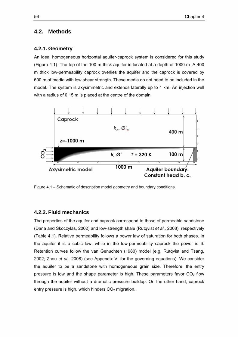
56 Chapter 4
4.2. Methods
4.2.1. Geometry An ideal homogeneous horizontal aquifer-caprock system is considered for this study
(Figure 4.1). The top of the 100 m thick aquifer is located at a depth of 1000 m. A 400
m thick low-permeability caprock overlies the aquifer and the caprock is covered by
600 m of media with low shear strength. These media do not need to be included in the
model. The system is axysimmetric and extends laterally up to 1 km. An injection well
with a radius of 0.15 m is placed at the centre of the domain.
Figure 4.1 – Schematic of description model geometry and boundary conditions.
4.2.2. Fluid mechanics The properties of the aquifer and caprock correspond to those of permeable sandstone
(Dana and Skoczylas, 2002) and low-strength shale (Rutqvist et al., 2008), respectively
(Table 4.1). Relative permeability follows a power law of saturation for both phases. In
the aquifer it is a cubic law, while in the low-permeability caprock the power is 6.
Retention curves follow the van Genuchten (1980) model (e.g. Rutqvist and Tsang,
2002; Zhou et al., 2008) (see Appendix VI for the governing equations). We consider
the aquifer to be a sandstone with homogeneous grain size. Therefore, the entry
pressure is low and the shape parameter is high. These parameters favor CO2 flow
through the aquifer without a dramatic pressure buildup. On the other hand, caprock
entry pressure is high, which hinders CO2 migration.
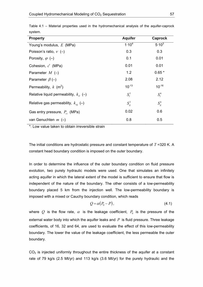
Coupled Hydromechanical Modeling of CO2 Sequestration 57
Table 4.1 – Material properties used in the hydromechanical analysis of the aquifer-caprock
system.
Property Aquifer Caprock
Young’s modulus, E (MPa) 1·104 5·103
Poisson’s ratio, ν (–) 0.3 0.3
Porosity, ϕ (–) 0.1 0.01
Cohesion, c′ (MPa) 0.01 0.01
Parameter M (–) 1.2 0.65 *
Parameter β (–) 2.08 2.12
Permeability, k (m2) 10-13 10-16
Relative liquid permeability, rlk (–) 3lS 6
lS
Relative gas permeability, rgk (–) 3gS 6
gS
Gas entry pressure, ccP (MPa) 0.02 0.6
van Genuchten m (–) 0.8 0.5
*: Low value taken to obtain irreversible strain
The initial conditions are hydrostatic pressure and constant temperature of T =320 K. A
constant head boundary condition is imposed on the outer boundary.
In order to determine the influence of the outer boundary condition on fluid pressure
evolution, two purely hydraulic models were used. One that simulates an infinitely
acting aquifer in which the lateral extent of the model is sufficient to ensure that flow is
independent of the nature of the boundary. The other consists of a low-permeability
boundary placed 5 km from the injection well. The low-permeability boundary is
imposed with a mixed or Cauchy boundary condition, which reads
( )PPQ −= 0α , (4.1)
where Q is the flow rate, α is the leakage coefficient, 0P is the pressure of the
external water body into which the aquifer leaks and P is fluid pressure. Three leakage
coefficients, of 16, 32 and 64, are used to evaluate the effect of this low-permeability
boundary. The lower the value of the leakage coefficient, the less permeable the outer
boundary.
CO2 is injected uniformly throughout the entire thickness of the aquifer at a constant
rate of 79 kg/s (2.5 Mt/yr) and 113 kg/s (3.6 Mt/yr) for the purely hydraulic and the

58 Chapter 4
coupled hydromechanical simulations, respectively. The latter falls within the range of
the CO2 generated by a 400 MW coal-fired power plant.
As for the fluid properties, the formation brine, at the aquifer depths considered, has an
initial density of 1087.5 kg/m3 and a viscosity of 6·10-4 Pa·s. Brine density depends on
pressure, temperature and the amount of dissolved CO2 in the brine. Brine viscosity
depends only on temperature and is therefore constant for the isothermal case
presented here. CO2 density is calculated using the formulas of Span and Wagner
(1996) and can vary significantly with pressure at the considered temperature T =320
K. The viscosity of CO2 depends on temperature and CO2 density (pressure). In this
study, it is calculated with an expression proposed by Altunin and Sakhabetdinov
(1972).
4.2.3. Geomechanics The initial stress field displays a greater vertical than horizontal stress, vh σσ ′=′ 65.0 ,
where vσ′ is the lithostatic effective stress. The mechanical boundary conditions are no
displacement normal to the bottom and outer boundary. A constant, vertical lithostatic
stress is imposed at the top of the caprock. We account for direct HM coupling, but we
do not include strain dependent hydraulic properties.
The viscoplastic constitutive model adopted here is conceptually appropriate and
computationally advantageous (Zienkiewicz and Cormeau, 1974; Zienkiewicz and
Taylor, 2000). Most rocks present a very small yield stress. Furthermore, a significant
pressure buildup will take place during CO2 sequestration. Therefore, irreversible
strains are expected to occur. This leads to the division of total strain into two parts ie εεε ddd += , (4.2)
where eε is the elastic strain tensor and iε is the inelastic strain tensor.
The yield criterion is formulated in terms of invariants of the effective stress tensor
( ) fzyx Ppp −=′+′+′=′ σσσ31
(4.3)
and
( ) 2t2 3
1:tr21 qJ == ss , (4.4)

Coupled Hydromechanical Modeling of CO2 Sequestration 59
where p′ is the mean effective stress, p is the mean stress, ( )wgf PPP ,max= is fluid
pressure, gP is the gas pressure, wP the water pressure and σ ′ denotes the effective
stress. 2J is the second invariant of Iσs p′−′= and then q is the equivalent deviatoric
stress. The superscript t denotes transpose. The sign convention of soil mechanics is
adopted, i.e. 0>p represents compression.
The elastic strain increments can be decomposed into a volumetric strain and a
deviatoric strain
Kpεev′
=dd , (4.5a)
Gqe
d 3dd =ε , (4.5b)
where evε and e
dε are the elastic volumetric strain and elastic deviatoric strain
respectively, ( )( )ν213/ −= EK is the bulk modulus, E is Young’s modulus, ν is the
Poisson ratio and ( )( )ν+= 12/EG is the shear modulus.
For the viscoplastic model, we adopted a Drucker-Prager yield function, F , defined as
βcMpqF −−= ' , (4.6)
where c is the cohesion and parameters M and β depend on the initial stress. For
compression ( 321 σσσ => )
'sin3'sin6φφ
−=M
'sin3'cos6φφβ
−= (4.7)
and for extension ( 321 σσσ >= )
'sin3'sin6φφ
+=M
'sin3'cos6φφβ
+= , (4.8)
where 'φ is the internal friction angle and c the cohesion, using the analogy with the
Mohr-Coulomb yield criterion. 0<F denotes elastic behaviour, and 0≥F implies
viscoplastic strain, which are defined as
( )σ
ε′∂
∂ΦΓ=
GFdtd i
, (4.9)
where t is time, Γ is a viscosity parameter, ( )FΦ is a stress function, σ′ is the
effective stress tensor and G is the flow rule, which is given by
)'( βα cMpqG +−= , (4.10)
60 Chapter 4
where α is a non-associativity parameter. The non-associativity parameter α can vary
between 0 and 1. When α is zero, there is no dilatancy, and when α equals one, the
model is associated and gives large dilatancy. In this study we consider α =0.3.
Finally, the stress function is defined as
( ) mFF =Φ , (4.11)
where m is a constant power, which has been chosen as 3 for this study. It should be
pointed out that both Γ and m are arbitrary in the sense that we are looking for an
irreversible strain, which is not time dependent, and which essentially depends on the
failure criteria. The analogy between viscoplasticity and plasticity is obtained from
( )σσ
ε′∂
∂Λ=
′∂∂
ΦΓ=GGdtFd i , (4.12)
where Λ would be the plastic multiplier. So, for a sufficiently large Γ , the plasticity
solution is recovered.
Mechanical failure can be assessed once the evolution of fluid pressure and related
changes in the stress field are known. As stated in the introduction, two failure
mechanisms can occur: hydraulic fracture and shear slip of pre-existing fractures.
Hydraulic fracture occurs when fluid pressure exceeds the least compressive principal
stress. This is a conservative assumption (Rutqvist et al., 2008) allowing for a safety
factor. Thus, the critical pressure for hydrofracturing would be for a fracture with
tension strength equal to zero
3σ≥fP . (4.13)
As for the onset of shear slip, if a fracture of random orientation exists at any point,
shear initiates plasticity when the deviatoric invariant q exceeds the yield function, i.e.
βcMpq +≥ ' . (4.14)
The two conditions can also be put together for an existing fracture without cohesion
using the following condition
0'≥−= MpqF . (4.15)

Coupled Hydromechanical Modeling of CO2 Sequestration 61
4.2.4. Numerical solution The injection of CO2 into a homogeneous saline aquifer is simulated using the finite
element numerical code CODE_BRIGHT (Olivella et al., 1994, 1996) modified for CO2
injection. Quadrilateral elements are used to enable the calculation of the mechanical
problem. The mesh, which is unstructured, consists of elements 10 m by 10 m located
close to the injection well, both in the aquifer and the caprock. The size of element
increases progressively away from the well up to a size of 30 m by 30 m at the outer
boundary. As a first step, a steady-state calculation is carried out to ensure equilibrium
for the pressure and stress fields.
4.3. Fluid pressure evolution
4.3.1. Infinitely acting aquifer Figure 4.2 displays the evolution of fluid pressure at the top of the injection well for an
infinitely acting aquifer. The magnitude of the pressure buildup is inversely proportional
to the permeability of the aquifer. Thus, the permeability of the aquifer may be a limiting
factor. Injection pressure increases sharply when CO2 injection starts. This sharp
increase is maintained while a capillary fringe is being formed. This is because the
relative permeability becomes very small when the porous media begins to desaturate.
Once the capillary fringe is fully developed, pressure begins to drop (see Appendix VII).
At this stage, the pores in the vicinity of the well are filled with CO2. Thus the fluid can
flow more easily, because CO2 viscosity is one order of magnitude smaller than that of
brine. The less viscous CO2 displaces the brine and the capillary fringe laterally. The
overpressure caused by the permeability reduction within the capillary fringe due to
desaturation decreases with distance from the injection well (Figure 4.3). This results in
a drop in fluid pressure buildup. This tendency is maintained until the CO2-water
interface is far enough so that the pressure drop due to the capillary fringe does not
influence injection. This may occur for very long injection times (see Appendix VII).
Thereafter, fluid pressure starts increasing slightly.
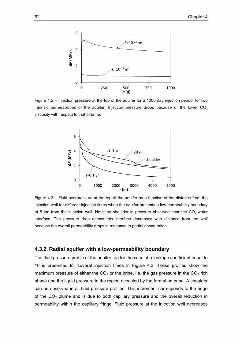
62 Chapter 4
0
2
4
6
0 250 500 750 1000
ΔP(M
Pa)
t (d)
k=10‐12 m2
k=10‐13 m2
Figure 4.2 – Injection pressure at the top of the aquifer for a 1000 day injection period, for two
intrinsic permeabilities of the aquifer. Injection pressure drops because of the lower CO2
viscosity with respect to that of brine.
0
2
4
6
0 1000 2000 3000 4000 5000
ΔP(M
Pa)
r (m)
t=30 yrt=1 yr
t=0.1 yr
shoulder
Figure 4.3 – Fluid overpressure at the top of the aquifer as a function of the distance from the
injection well for different injection times when the aquifer presents a low-permeability boundary
at 5 km from the injection well. Note the shoulder in pressure observed near the CO2-water
interface. The pressure drop across this interface decreases with distance from the well
because the overall permeability drops in response to partial desaturation.
4.3.2. Radial aquifer with a low-permeability boundary The fluid pressure profile at the aquifer top for the case of a leakage coefficient equal to
16 is presented for several injection times in Figure 4.3. These profiles show the
maximum pressure of either the CO2 or the brine, i.e. the gas pressure in the CO2 rich
phase and the liquid pressure in the region occupied by the formation brine. A shoulder
can be observed in all fluid pressure profiles. This increment corresponds to the edge
of the CO2 plume and is due to both capillary pressure and the overall reduction in
permeability within the capillary fringe. Fluid pressure at the injection well decreases
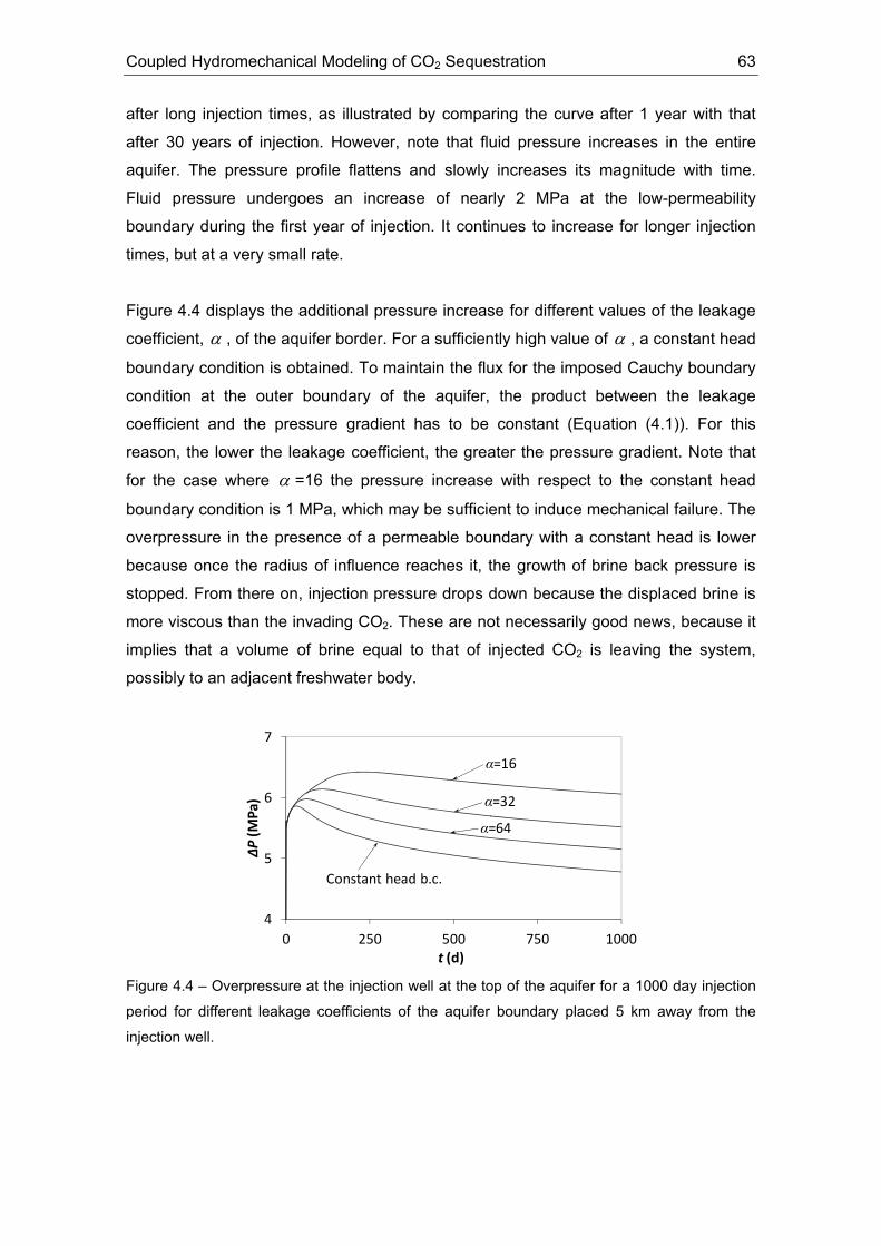
Coupled Hydromechanical Modeling of CO2 Sequestration 63
after long injection times, as illustrated by comparing the curve after 1 year with that
after 30 years of injection. However, note that fluid pressure increases in the entire
aquifer. The pressure profile flattens and slowly increases its magnitude with time.
Fluid pressure undergoes an increase of nearly 2 MPa at the low-permeability
boundary during the first year of injection. It continues to increase for longer injection
times, but at a very small rate.
Figure 4.4 displays the additional pressure increase for different values of the leakage
coefficient, α , of the aquifer border. For a sufficiently high value of α , a constant head
boundary condition is obtained. To maintain the flux for the imposed Cauchy boundary
condition at the outer boundary of the aquifer, the product between the leakage
coefficient and the pressure gradient has to be constant (Equation (4.1)). For this
reason, the lower the leakage coefficient, the greater the pressure gradient. Note that
for the case where α =16 the pressure increase with respect to the constant head
boundary condition is 1 MPa, which may be sufficient to induce mechanical failure. The
overpressure in the presence of a permeable boundary with a constant head is lower
because once the radius of influence reaches it, the growth of brine back pressure is
stopped. From there on, injection pressure drops down because the displaced brine is
more viscous than the invading CO2. These are not necessarily good news, because it
implies that a volume of brine equal to that of injected CO2 is leaving the system,
possibly to an adjacent freshwater body.
4
5
6
7
0 250 500 750 1000
ΔP(M
Pa)
t (d)
Constant head b.c.
α=16
α=32
α=64
Figure 4.4 – Overpressure at the injection well at the top of the aquifer for a 1000 day injection
period for different leakage coefficients of the aquifer boundary placed 5 km away from the
injection well.

64 Chapter 4
For a low-permeability boundary located at a distance greater than the one considered
here, this fluid pressure increase behaviour would happen in the same manner, but
delayed a time equal to )25.2/(2 gkRS wsw ρμ , where R is the distance at which the
low-permeability boundary is located. If the low-permeability boundary was located at a
considerable distance from the injection well, the injection pressure would drop after
the initial increase (Figure 4.2). However, once the radius of influence of the injection
reached the low-permeability boundary, fluid pressure would increase in the whole
aquifer (Figure 4.3). In particular, fluid pressure would also increase again at the
injection well.
4.4. Hydromechanical coupling
CO2 injection causes fluid pressure to increase, thus changing the effective stress
tensor. The latter produces deformations of the medium, and these deformations exert
an influence on the evolution of fluid pressure. Figure 4.5 compares a purely hydraulic
simulation (H) with a coupled hydromechanical (HM) simulation of the model presented
in Figure 4.1. This coupled HM simulation uses the viscoplastic constitutive model
outlined in Section 4.2.3. The difference between the purely hydraulic and the coupled
hydromechanical simulations is small in the aquifer (Figure 4.5a). The two curves are
almost parallel, with comparable asymptotic values of the pressures, and can be
corrected by a translation, which depends on the storage coefficient selected.
However, it is not easy to assign storativity values because the real relationship
between stress and volumetric strain is very sensitive to strain mechanisms.
Furthermore, HM simulation captures porosity changes due to rock strain (not only
volumetric) in contrast to H simulation, which only considers a storage coefficient that
includes fluid and rock compressibility (Mainguy and Longuemare, 2002). Thus, the two
curves are not exactly parallel. Interestingly, the difference becomes significant in the
caprock (Figure 4.5b). Hydraulic simulations do not capture the drop in the initial fluid
pressure because of mechanical effects, such as dilatancy or bending of the caprock
due to CO2 injection. Thus, measuring fluid pressure in the caprock plays a major role
in identifying the hydromechanical processes.
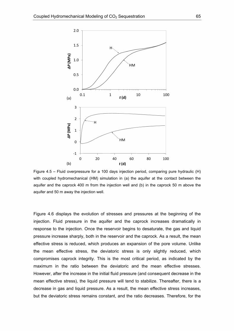
Coupled Hydromechanical Modeling of CO2 Sequestration 65
0.0
0.5
1.0
1.5
2.0
0.1 1 10 100
ΔP (M
Pa)
t (d)
HM
H
(a)
‐1
0
1
2
3
0 20 40 60 80 100
ΔP(M
Pa)
t (d)
HM
H
(b) Figure 4.5 – Fluid overpressure for a 100 days injection period, comparing pure hydraulic (H)
with coupled hydromechanical (HM) simulation in (a) the aquifer at the contact between the
aquifer and the caprock 400 m from the injection well and (b) in the caprock 50 m above the
aquifer and 50 m away the injection well.
Figure 4.6 displays the evolution of stresses and pressures at the beginning of the
injection. Fluid pressure in the aquifer and the caprock increases dramatically in
response to the injection. Once the reservoir begins to desaturate, the gas and liquid
pressure increase sharply, both in the reservoir and the caprock. As a result, the mean
effective stress is reduced, which produces an expansion of the pore volume. Unlike
the mean effective stress, the deviatoric stress is only slightly reduced, which
compromises caprock integrity. This is the most critical period, as indicated by the
maximum in the ratio between the deviatoric and the mean effective stresses.
However, after the increase in the initial fluid pressure (and consequent decrease in the
mean effective stress), the liquid pressure will tend to stabilize. Thereafter, there is a
decrease in gas and liquid pressure. As a result, the mean effective stress increases,
but the deviatoric stress remains constant, and the ratio decreases. Therefore, for the
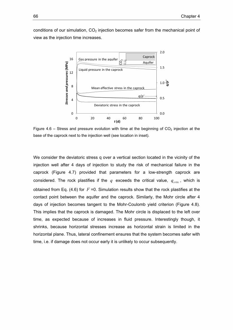
66 Chapter 4
conditions of our simulation, CO2 injection becomes safer from the mechanical point of
view as the injection time increases.
0.0
0.5
1.0
1.5
2.0
0
4
8
12
16
0 20 40 60 80 100
q/p'
Stresses and
pressures (M
Pa)
t (d)
Gas pressure in the aquifer
Liquid pressure in the caprock
Mean effective stress in the caprock
Deviatoric stress in the caprock
q/p'
CO2
Aquifer
Caprock
Figure 4.6 – Stress and pressure evolution with time at the beginning of CO2 injection at the
base of the caprock next to the injection well (see location in inset).
We consider the deviatoric stress q over a vertical section located in the vicinity of the
injection well after 4 days of injection to study the risk of mechanical failure in the
caprock (Figure 4.7) provided that parameters for a low-strength caprock are
considered. The rock plastifies if the q exceeds the critical value, criticq , which is
obtained from Eq. (4.6) for F =0. Simulation results show that the rock plastifies at the
contact point between the aquifer and the caprock. Similarly, the Mohr circle after 4
days of injection becomes tangent to the Mohr-Coulomb yield criterion (Figure 4.8).
This implies that the caprock is damaged. The Mohr circle is displaced to the left over
time, as expected because of increases in fluid pressure. Interestingly though, it
shrinks, because horizontal stresses increase as horizontal strain is limited in the
horizontal plane. Thus, lateral confinement ensures that the system becomes safer with
time, i.e. if damage does not occur early it is unlikely to occur subsequently.

Coupled Hydromechanical Modeling of CO2 Sequestration 67
‐1000
‐900
‐800
‐700
‐600
0 2 4 6 8
z(m
)
Deviatoric stress (MPa)
qcriticq
Figure 4.7 – A vertical section of the caprock in the vicinity of the well, with the deviatoric stress,
q , and critical the deviatoric stress, criticq , after 4 days of injection. Note that q exceeds criticq
in the contact between the caprock and the aquifer, thus causing the caprock to plastify.
0.0
1.5
3.0
4.5
6.0
0 4 8 12
τ(MPa)
σ' (MPa)
Mohr‐Coulomb failure criterion (M=0.65)
t=4 d
t=0 d
Figure 4.8 – Mohr circles at the initial state and after 4 days of injection. The parameters of the
Mohr-Coulomb failure criterion are c =0 and φ′=17.2º (low value taken to obtain irreversible
strain). The Mohr circle after 4 days of injection is displaced to the left (reduction in p′ ) and is
reduced in size (reduction in q ).
This behaviour is also observed in the ( q , p′ ) plane for a point at the base of the
caprock close to the well over an injection period of 100 days (Figure 4.9). Prior to
injection (point A), the caprock is in the safe zone, at some distance from the plastic
regime. Once injection begins, the mean effective stress decreases much more
drastically than the deviatoric stress and the Mohr-Coulomb yield envelope is rapidly
reached (point B). At this point, the rock begins to behave plastically. Thus, strain
occurs plastically for a few days, until it reaches point C after 5 days of injection. Then,
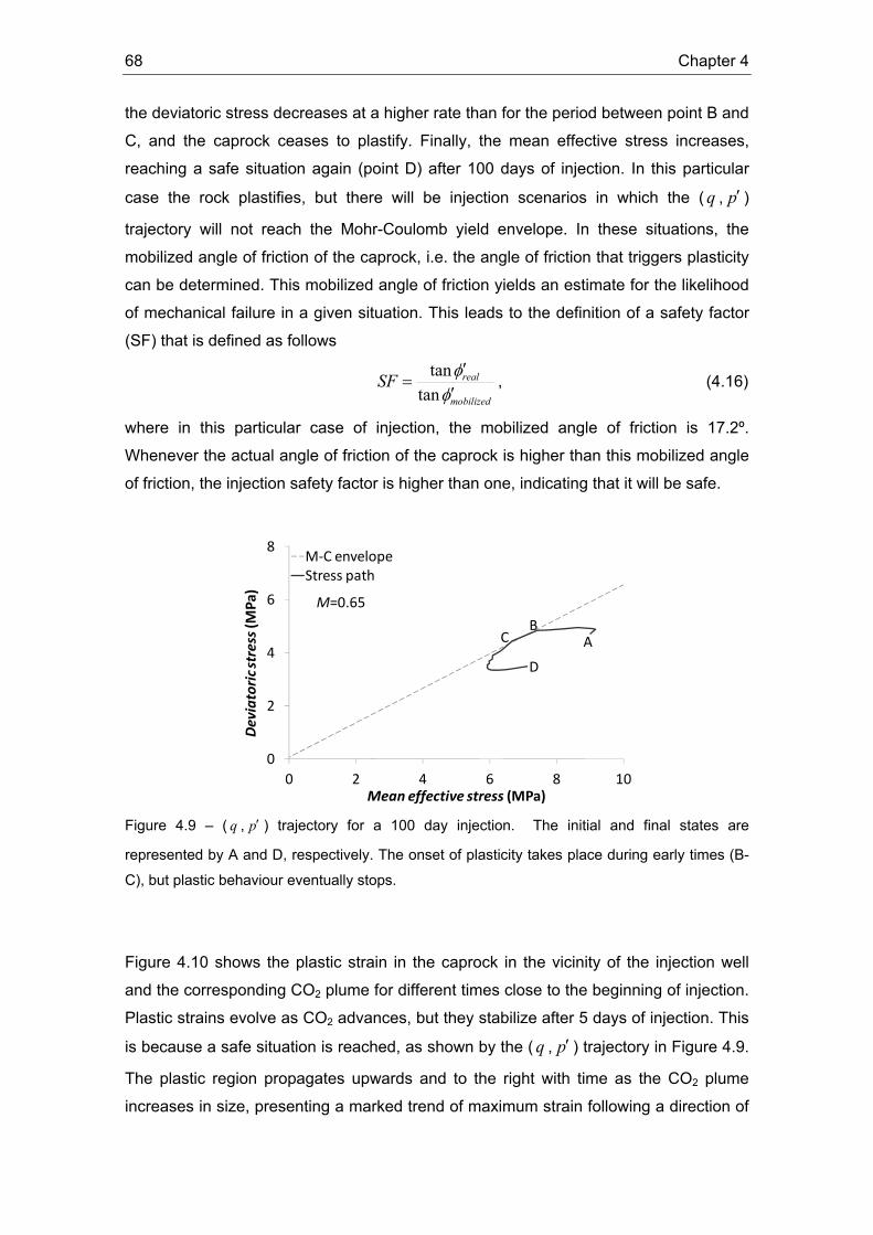
68 Chapter 4
the deviatoric stress decreases at a higher rate than for the period between point B and
C, and the caprock ceases to plastify. Finally, the mean effective stress increases,
reaching a safe situation again (point D) after 100 days of injection. In this particular
case the rock plastifies, but there will be injection scenarios in which the (q , p′ )
trajectory will not reach the Mohr-Coulomb yield envelope. In these situations, the
mobilized angle of friction of the caprock, i.e. the angle of friction that triggers plasticity
can be determined. This mobilized angle of friction yields an estimate for the likelihood
of mechanical failure in a given situation. This leads to the definition of a safety factor
(SF) that is defined as follows
mobilized
realSFφφ′′
=tan
tan, (4.16)
where in this particular case of injection, the mobilized angle of friction is 17.2º.
Whenever the actual angle of friction of the caprock is higher than this mobilized angle
of friction, the injection safety factor is higher than one, indicating that it will be safe.
0
2
4
6
8
0 2 4 6 8 10
Deviatoric stress (M
Pa)
Mean effective stress (MPa)
M‐C envelopeStress path
AB
C
D
M=0.65
Figure 4.9 – ( q , p′ ) trajectory for a 100 day injection. The initial and final states are
represented by A and D, respectively. The onset of plasticity takes place during early times (B-
C), but plastic behaviour eventually stops.
Figure 4.10 shows the plastic strain in the caprock in the vicinity of the injection well
and the corresponding CO2 plume for different times close to the beginning of injection.
Plastic strains evolve as CO2 advances, but they stabilize after 5 days of injection. This
is because a safe situation is reached, as shown by the (q , p′ ) trajectory in Figure 4.9.
The plastic region propagates upwards and to the right with time as the CO2 plume
increases in size, presenting a marked trend of maximum strain following a direction of

Coupled Hydromechanical Modeling of CO2 Sequestration 69
approximately 45º to the ground surface. Once this plastic region stabilizes, it reaches
horizontally a distance of 175 m from the injection well and 125 m above the base of
the caprock. Note that the induced plastic strains are small (0.04 %), which suggests
that the integrity of the caprock will not be compromised here.
Figure 4.10 – Plastic strain (EDP) in the caprock (left) and liquid saturation degree, lS , in the
aquifer (right) for different injection times. Plastic strain propagates as CO2 advances at the
beginning of injection.
Unlike horizontal displacements, vertical displacements can be significant (Vasco et al.,
2008; Rutqvist et al., 2010). Figure 4.11 shows the vertical displacement that takes
place at the top of the caprock, at a depth of 600 m, as a function of the distance from
the injection well at different injection times. The vertical displacement has a typical bell
shape. The magnitude of the uplift gradually increases with time, reaching a maximum
of several centimeters next to the injection well after 100 days of injection. This
particular model does not simulate the upper 600 m of rock, but the vertical
displacement should follow a similar trend, which means that a significant uplift of the
ground could take place (Morris et al., 2009).

70 Chapter 4
0
10
20
30
40
0 250 500 750 1000
Vertical Displacem
ent (mm)
r (m)
t=100 d
t=40 d
t=15 d
t=5 d
Upper layer
Aquifer
Caprock
CO2
‐600 m
Figure 4.11 – Vertical displacement as a function of distance from the well for different injection
times at the top of the caprock ( z = -600 m).
4.5. Discussion and conclusions
We conducted simulations of CO2 injection into a deep saline aquifer to study the risk
of caprock mechanical failure. The specific scenario we model is meant to reflect a real
world scenario. In particular, we assumed the material to be viscoplastic and the initial
stress tensor to be axysimmetric with the vertical stress greater than the horizontal
ones.
Given that instability is caused by fluid pressure buildup, we carried out hydraulic
simulations of an infinitely acting aquifer and a circular aquifer with a low-permeability
boundary to study the influence of the boundary condition. Exclusion of the mechanical
component allowed us to run the simulations at a reasonably low computational cost.
We found that after an initial sharp increase, the fluid pressure drops. This occurs
because the less viscous CO2 displaces brine and the capillary fringe laterally. This
capillary fringe produces an overpressure because of permeability reduction due to
desaturation. This overpressure decreases with distance from the injection well. Thus,
fluid pressure decreases with time. This drop in fluid pressure may allow the injection of
an additional amount of CO2 without compromising the caprock stability. Furthermore,
the measurement of this fluid pressure drop in field tests (with constant injection mass
rate) can give valuable information about the capillary fringe.
If the aquifer has a low-permeability boundary, fluid pressure can rise again once the
Coupled Hydromechanical Modeling of CO2 Sequestration 71
radius of influence reaches this boundary. This increase takes place in the whole
aquifer. This additional overpressure may induce rock failure in the long term. In most
CO2 sequestration projects, the boundaries of the basins will play a role in the injection
since CO2 sequestration projects are planned to take place over long periods of time
(several decades). Over such timescales the radius of influence will reach tens and
even hundreds of kilometers, depending on the permeability of the aquifer. Thus, the
geometry and hydraulic properties of the aquifer boundaries should be characterized in
detail.
Full coupling in hydromechanical simulations leads to lower increases in fluid pressure
than the use of purely hydraulic simulations. This occurs because of rock deformations.
The difference can be small in the aquifer if a good estimate of the storage coefficient
is used. However, the evolution of fluid pressure is completely different in the caprock
because of mechanical effects such as dilatancy and bending of the caprock due to
CO2 injection. In these coupled simulations we consider direct HM couplings, but not
indirect HM ones (such as changes in permeability due to porosity changes (Rutqvist
and Tsang, 2002)). The incorporation of indirect HM couplings might lead to significant
differences in the results. On the other hand, direct HM couplings consider rock strain
and changes in the stress field (Figure 4.8). CO2 injection increases fluid pressure and
as a result the rock deforms leading to changes in the porosity. This deformation
increases the pore volume, resulting in a drop in fluid pressure. Despite this drop in
fluid pressure, a sufficiently large overpressure occurs in the reservoir, inducing plastic
strain in the caprock at the beginning of the injection. In this work, the caprock
mechanical strength was intentionally chosen so that the rock plastifies as our goal was
to determine failure mechanisms that could serve as an escape route for CO2.
In practice, it is essential to determine the in situ stress field. The failure mechanisms
discussed here could be expected for cases where the vertical stress is greater than
the horizontal stresses. From a mechanical perspective, the analysis of the ( q , p′ )
trajectories illustrates that the most critical period occurs in the early stages for a
constant injection rate. The stress state can be close to failure during this period.
Failure will occur when the yield surface is reached, giving rise to plastic strain, which
may result in microfracturing (i.e. detectable by a local seismic network). Yield is local,
so that the breakup of caprock is unlikely. Nonetheless, monitoring caprock integrity at
the beginning of the injection is crucial to ensure a safe injection. As shown in Figure
4.10, the caprock could yield at the beginning of the injection and the damage could
propagate through a portion of the caprock. Furthermore, if a weak zone was already

72 Chapter 4
present in the caprock, the damage would be greater and preferential paths could be
created, allowing the CO2 to migrate up to shallow aquifers or even the ground surface.
If the CO2 can penetrate into the caprock, geochemical interactions will take place due
to its acidity.
To limit local failure at the beginning of injection, a good characterization of the caprock
is necessary. If the strength of the rock was known, numerical simulations would
enable us to determine a sustainable injection pressure. This may be achieved by
determining the mobilized angle of friction and by ensuring that it does not exceed the
real friction angle of the rock even in weak zones. The use of a safety factor (Equation
(4.16)) can be valuable in probabilistic risk assessment (e.g. Tartakovsky, 2007;
Bolster et al., 2009a; Jurado et al., 2012).
In this study, a homogeneous caprock is considered. Heterogeneities in the caprock,
such as weak zones, fractured zones or discontinuities, are likely to be present in most
injection areas. Furthermore, given that CO2 injection projects are planned to last
decades, the CO2 plume will span several kilometers. Therefore, future studies should
address the influence of mechanical and hydraulic heterogeneities in the caprock in
order to simulate more realistic situations.
We modified and used the program CODE_BRIGHT to study the coupled
hydromechanical evolution in an aquifer-caprock system during CO2 sequestration in
deep saline aquifers. In summary, the main conclusions drawn from this study are:
- Fluid pressure begins to drop once the capillary fringe is fully developed. The
overpressure produced within the capillary fringe (because of permeability
reduction due to desaturation) decreases with the distance from the well.
Measuring this fluid pressure drop in field tests can give valuable information
about the capillary fringe. Furthermore, an additional amount of CO2 may be
injected with a small increase in fluid pressure.
- If the aquifer has a low-permeability boundary, fluid pressure can rise once the
radius of influence reaches the outer boundary. As a result of this, the
mechanical integrity of the caprock could be compromised in the long term.
- The lower zone of the caprock presents the largest hydromechanical changes,
presenting the greatest risk of rock failure, particularly in the early stages of
injection.
Coupled Hydromechanical Modeling of CO2 Sequestration 73
- Slowly increasing the injection rate at the beginning of injection is
recommendable in order to reduce possible damage to the caprock.
Furthermore, measuring fluid pressure in the caprock is essential for identifying
hydromechanical processes.
Numerical simulations allow us to estimate the maximum sustainable injection pressure
given the strength of the caprock. A safety factor can be defined by determining the
mobilized angle of friction.


75
5. Hydromechanical Characterization
of CO2 Injection Sites
5.1. Introduction
Coupled hydromechanical effects, such as ground deformation, induced
microseismicity and fault reactivation, should be understood and quantified to
demonstrate to the public that geologic carbon storage is safe. The most representative
example of a coupled hydromechanical effect may be the ground heave of 0.5 mm/yr
on top of the carbon dioxide (CO2) injection wells at the In Salah storage project in
Algeria (Rutqvist et al., 2010; Vasco et al., 2010). Other relevant examples are related
to induced microseismicity and seismicity. Induced microseismic events were detected
at Otsego County, Michigan Basin, US, due to CO2 leakage around wells (Bohnhoff et
al., 2010) and in the Weyburn field, Saskatchewan, Canada (Verdon et al., 2011).
Cappa and Rutqvist (2011b) estimated through numerical simulations that CO2
injection in a deep aquifer bounded by a low-permeability fault can trigger earthquakes
with magnitude up to 4.5. Additionally, a natural high pressure CO2 source is believed
to have driven, after the occurrence of two earthquakes, thousands of aftershocks in
the Northern Apennines, Italy, during more than 30 days, including four events with
moment magnitudes ranging from 5 to 6 (Miller et al., 2004). Thus, hydromechanical
processes need to be well understood to ensure stable permanent CO2 storage in deep
geological formations.
Hydromechanical studies have focused on several aspects, including the estimation of
maximum sustainable injection pressure (Streit and Hillis, 2004; Rutqvist et al., 2007),
evaluating fault reactivation due to production of gas/oil fields (Ferronato et al., 2008;
Soltanzadeh and Hawkes, 2009) and due to CO2 injection (Ferronato et al., 2010;
Cappa and Rutqvist, 2011a). Fault reactivation occurs once the fault yields, in which
case induced microsesimicity will be triggered. This microseismicity is usually due to
shear-slip and produces changes in the fault aperture in the order of microns (Guglielmi
et al. 2008). Thus, fracture permeability is enhanced, especially in the direction
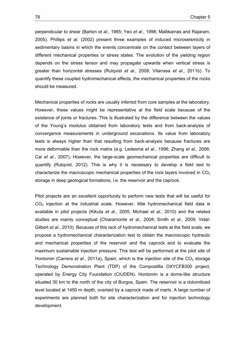
76 Chapter 5
perpendicular to shear (Barton et al., 1985; Yeo et al., 1998; Mallikamas and Rajaram,
2005). Phillips et al. (2002) present three examples of induced microseismicity in
sedimentary basins in which the events concentrate on the contact between layers of
different mechanical properties or stress states. The evolution of the yielding region
depends on the stress tensor and may propagate upwards when vertical stress is
greater than horizontal stresses (Rutqvist et al., 2008; Vilarrasa et al., 2011b). To
quantify these coupled hydromechanical effects, the mechanical properties of the rocks
should be measured.
Mechanical properties of rocks are usually inferred from core samples at the laboratory.
However, these values might be representative at the field scale because of the
existence of joints or fractures. This is illustrated by the difference between the values
of the Young’s modulus obtained from laboratory tests and from back-analysis of
convergence measurements in underground excavations. Its value from laboratory
tests is always higher than that resulting from back-analysis because fractures are
more deformable than the rock matrix (e.g. Ledesma et al., 1996; Zhang et al., 2006;
Cai et al., 2007). However, the large-scale geomechanical properties are difficult to
quantify (Rutqvist, 2012). This is why it is necessary to develop a field test to
characterize the macroscopic mechanical properties of the rock layers involved in CO2
storage in deep geological formations, i.e. the reservoir and the caprock.
Pilot projects are an excellent opportunity to perform new tests that will be useful for
CO2 injection at the industrial scale. However, little hydromechanical field data is
available in pilot projects (Kikuta et al., 2005; Michael et al., 2010) and the related
studies are mainly conceptual (Chiaramonte et al., 2008; Smith et al., 2009; Vidal-
Gilbert et al., 2010). Because of this lack of hydromechanical tests at the field scale, we
propose a hydromechanical characterization test to obtain the macroscopic hydraulic
and mechanical properties of the reservoir and the caprock and to evaluate the
maximum sustainable injection pressure. This test will be performed at the pilot site of
Hontomin (Carrera et al., 2011a), Spain, which is the injection site of the CO2 storage
Technology Demonstration Plant (TDP) of the Compostilla OXYCFB300 project,
operated by Energy City Foundation (CIUDEN). Hontomin is a dome-like structure
situated 30 km to the north of the city of Burgos, Spain. The reservoir is a dolomitized
level located at 1450 m depth, overlaid by a caprock made of marls. A large number of
experiments are planned both for site characterization and for injection technology
development.
Hydromechanical Characterization Test 77
5.2. Mechanical properties of rocks
Sedimentary rocks (sandstone, limestone and dolomite) are potential host rocks for
CO2 storage. On the other hand, low-permeability, high-entry pressure formations, such
as shale, marl and claystone, can form the caprock. Mechanical properties of these
rock types (Figures 5.1 and 5.2) can take a wide range of values.
0
0.1
0.2
0.3
0.4
0.5
0 10 20 30 40 50 60
Poisson ratio
Young's modulus (GPa)
Berea Sandstone Adamswiller SandstoneRed Sandstone Bentheim SandstoneDarley Dale Sandstone Solenhofen LimestoneBedford Limestone Tavernalle LimestoneLavoux Limestone ShaleWoodford Shale Oil ShaleMuderong Shale Boom ClayOpalinus Clay Callovo‐Oxfordian ShalePuerto Rico Shale Dolomitic Marble
Figure 5.1 – Literature review of matrix Young’s modulus and Poisson ratio for several
sandstones, limestones, dolomitic marble and shales.
The variation in rock properties depends on the rock type. For example, the Young’s
modulus of sandstones and limestones ranges only from 1 to 20 GPa (Goodman,
1989; Abousleiman et al., 2010; Heap et al., 2010; Hu et al., 2010; Rimmele et al.,
2010). Instead, reported Young’s moduli of shales range over two orders of magnitude.
Soft shales, like the Boom Clay, display Young’s moduli in the order of 0.1-0.4 GPa
(Giraud and Rousset, 1996; Mertens et al., 2004; Dehandschutter et al., 2005; François
et al., 2009). Stiff clays, like one from Puerto Rico, have got Young’s moduli in the
order of 20-40 GPa (Shalabi et al., 2007). Other shales (Ortega et al., 2010), such as
oil shales (Eseme et al., 2007), Opalinus Clay (Thury, 2002; Gens et al., 2007) and
Callovo-Oxfordian argillite (Zhang and Rothfuchs, 2004; Saurot et al., 2007; Wileveau
and Bernier, 2008), have intermediate Young’s modulus values, ranging from 1 to 20

78 Chapter 5
GPa. The actual value of the Young’s modulus increases with the mean effective stress
(Dodds et al., 2007; Shalabi et al., 2007; Hu et al., 2010).
0
10
20
30
0 10 20 30 40 50 60 70
Cohesion
(MPa)
Friction angle (°)
Berea SandstoneBartlesville SandstonePottsville SandstoneWolf Camp LimestoneIndiana LimestoneWoodford ShaleOil ShaleBoom ClayOpalinus ClayCallovo‐Oxfordian ShalePersian Gulf ShaleDark ShaleMarlHasmark Dolomite
Parallel to bedding
Perpendicular to bedding
Figure 5.2 – Literature review of cohesion and friction angle for several sandstones, limestones,
marls, dolomite and shales.
Poisson ratios range from 0.15 to 0.25 for the vast majority of rock samples (Figure
5.1). Some values close to 0.5 (incompressible) are reported in low-permeability rocks.
These values are due to undrained conditions, but they are not representative of the
real Poisson ratio of the rock.
The friction angle of existing fractures is important because it controls the occurrence
of microseismic events. Sedimentary formations, which are formed after depositional
sequences, present a high anisotropy in the directions parallel and perpendicular to
bedding (Thury, 2002; Gens et al., 2007; Saurot et al., 2007). Friction angles as low as
5° (Figure 5.2) have been found in the direction parallel to bedding in clay-rich
materials (Gens et al., 2007) or when the rock has been weakened due to
demineralization (Abousleiman et al., 2010). Related to this, the percentage of
carbonate in the clay-size material of marls affects the residual friction angle. Low
carbonate content (<11%) yields residual friction angles around 12°. High carbonate
content (>30%) yields residual friction angles around 30° (Frydman et al., 2007).
Hydromechanical Characterization Test 79
Figures 5.1 and 5.2 illustrate that the mechanical properties of sedimentary rocks are
highly variable. Additionally, these properties are difficult to estimate at the field scale,
which is the scale of interest for CO2 sequestration. Hydromechanical numerical
studies usually take the values obtained from samples tested at the laboratory as the
values of the formation. However, laboratory tests are representative of the rock matrix,
but not of the formation as a whole. This is because the formation is fractured. The
value of the Young’s modulus of the formation can differ in more than one order of
magnitude with respect to that of the matrix. For example, Verdon et al. (2011) had to
reduce the Young’s modulus of the aquifer from 14.5 (value obtained from laboratory
tests) to 0.5 GPa in order to adjust their model to the observed microseismicity in the
Weyburn field, Saskatchewan, Canada.
5.3. Hydromechanical characterization test
5.3.1. Test description We propose a test to characterize the hydromechanical parameters of the aquifer and
caprock at the field scale. The test consists in injecting water at high pressure and flow
rate, while monitoring fluid pressure, rock deformation and induced microseismicity
(Figure 5.3). The overpressure (several MPa) is proportional to the flow rate, which can
be high if the aquifer transmissivity is high. The injected water can be obtained from
surface sources, e.g. rivers or lakes. However, aquifer brine must be used if
geochemical alteration is not desired. In this case, brine is pumped and stored at the
surface prior to the injetion test. Therefore, the duration of the injection will be
conditioned by storage capacity.
The overpressure should be progressively increased until the elastic limit is reached
and microseismicity occurs. Microseisms can take place both in the reservoir and the
caprock. Since microseisms open up fractures, enhancing their transmissivity,
microseismicity will be benificial while it occurs within the aquifer. However, if it occurs
in the caprock, the maximum sustainable injection pressure is reached, indicating the
overpressure that must not be exceeded during the operational stage of CO2 injection.
Instrumentation for the test consists of equipments to measure fluid pressure, vertical
displacement and microseismicity. Fluid pressure and vertical displacement
measurements are taken in the injection and observation wells, both in the reservoir

80 Chapter 5
and the caprock (Figure 5.3). In the case that vertical displacement measurements are
not available, strain should be measured. An array of geophones should be placed in
the observation well at depth to detect microseismic events of magnitudes as low as -3.
Additionally, a network of geophones in surface can complement the microseismicity
measurements and help to localize the events. Microseismicity measurements are
essential to guarantee the caprock integrity and avoid leakage of future CO2 injection
tests in the same site.
Figure 5.3 – Schematic representation of the hydromechanical characterization test. A
sufficiently high water flow rate so as to reach the maximum sustainable injection pressure is
injected for several hours. Fluid pressure and displacements or strains are monitored in the
aquifer and caprock in as many places as possible (preferably in both the injection and the
observation well, but at least in one well).
5.3.2. Problem formulation
a) Elasticity in porous media
Fluid injection induces strain in the aquifer-caprock system, which will be elastic while
failure conditions are not reached. Hooke’s law gives the relationship between elastic
strain and effective stress, which can be written either as (Zimmerman, 2000)
( )IσIε pGK
m ′−′+′
=21
3σ , (5.1a)
or as
⎟⎠⎞
⎜⎝⎛ −+=′ IεIσ
32 v
v GK εε , (5.1b)
Hydromechanical Characterization Test 81
where ε is the elastic strain tensor, σ′ is the effective stress tensor,
( ) 3zyxm σσσσ ′+′+′=′ is the mean effective stress, I is the identity matrix,
( )( )ν213 −= EK is the bulk modulus, ( )( )ν+= 12EG is the shear modulus, E is the
Young’s modulus, ν the Poisson ratio and vε is volumetric strain.
Elastic strain can be decomposed into a volumetric and a deviatoric strain
Km
vσε′
= (5.2a)
Gq
d 3=ε (5.2b)
where dε is deviatoric strain, D
Jq 23= is deviatoric stress and ( ) ( )ss :tr212T
DJ = is
the second invariant of Iσs mσ ′−′= . Note that Eq. (5.1a) and (5.1b) are related through
Eq. (5.2a).
Considering the sign criterion of continuum mechanics, i.e. stress is positive in tension
and fluid pressure is positive in compression, the effective stress tensor is defined as
Iσσ p+=′ , (5.3)
where σ is the total stress tensor and p is fluid pressure.
To solve the mechanical problem, the momentum balance of the porous media has to
be satisfied. If the inertial terms are neglected, it reduces to the equilibrium of stresses
0bσ =+⋅∇ , (5.4)
where b is the vector of body forces.
Introducing Eq. (5.1b) and (5.3) in Eq. (5.4) gives the equilibrium of stresses in terms of
strain as
0bε =+∇−⋅∇+∇⎟⎠⎞
⎜⎝⎛ − pGGK v 2
32 ε . (5.5)
The compatibility relationship that relates strain to displacements reads
( )( )Tuuε ∇+∇=21 , (5.6)
where u is the displacement vector and the superscript T denotes transpose.
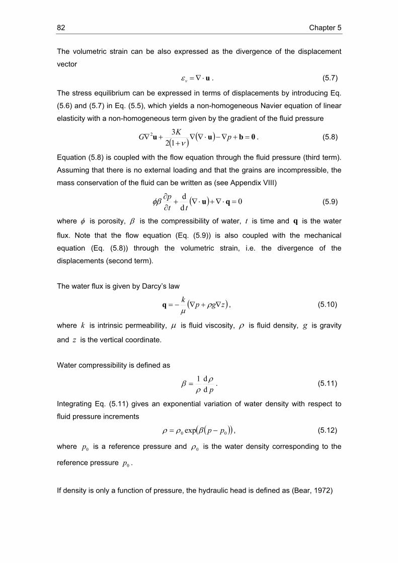
82 Chapter 5
The volumetric strain can be also expressed as the divergence of the displacement
vector
u⋅∇=vε . (5.7)
The stress equilibrium can be expressed in terms of displacements by introducing Eq.
(5.6) and (5.7) in Eq. (5.5), which yields a non-homogeneous Navier equation of linear
elasticity with a non-homogeneous term given by the gradient of the fluid pressure
( ) ( ) 0buu =+∇−⋅∇∇+
+∇ pKGν12
32 . (5.8)
Equation (5.8) is coupled with the flow equation through the fluid pressure (third term).
Assuming that there is no external loading and that the grains are incompressible, the
mass conservation of the fluid can be written as (see Appendix VIII)
( ) 0dd
=⋅∇+⋅∇+∂∂ qu
ttpφβ (5.9)
where φ is porosity, β is the compressibility of water, t is time and q is the water
flux. Note that the flow equation (Eq. (5.9)) is also coupled with the mechanical
equation (Eq. (5.8)) through the volumetric strain, i.e. the divergence of the
displacements (second term).
The water flux is given by Darcy’s law
( )zgpk∇+∇−= ρ
μq , (5.10)
where k is intrinsic permeability, μ is fluid viscosity, ρ is fluid density, g is gravity
and z is the vertical coordinate.
Water compressibility is defined as
pdd1 ρ
ρβ = . (5.11)
Integrating Eq. (5.11) gives an exponential variation of water density with respect to
fluid pressure increments
( )( )00 exp pp −= βρρ , (5.12)
where 0p is a reference pressure and 0ρ is the water density corresponding to the
reference pressure 0p .
If density is only a function of pressure, the hydraulic head is defined as (Bear, 1972)
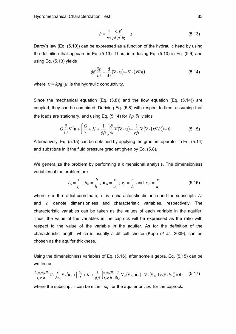
Hydromechanical Characterization Test 83
( )∫ +′′
=p
pz
gpph
0
dρ
. (5.13)
Darcy’s law (Eq. (5.10)) can be expressed as a function of the hydraulic head by using
the definition that appears in Eq. (5.13). Thus, introducing Eq. (5.10) in Eq. (5.9) and
using Eq. (5.13) yields
( ) ( )htt
p∇⋅∇=⋅∇+
∂∂ κφβ u
dd , (5.14)
where μρκ gk= is the hydraulic conductivity.
Since the mechanical equation (Eq. (5.8)) and the flow equation (Eq. (5.14)) are
coupled, they can be combined. Deriving Eq. (5.8) with respect to time, assuming that
the loads are stationary, and using Eq. (5.14) for tp ∂∂ yields
( ) ( )( ) 0uu =∇⋅∇∇−⋅∇∇∂∂
⎟⎟⎠
⎞⎜⎜⎝
⎛+++∇
∂∂ h
tKG
tG κ
φβφβ11
32 . (5.15)
Alternatively, Eq. (5.15) can be obtained by applying the gradient operator to Eq. (5.14)
and substitute in it the fluid pressure gradient given by Eq. (5.8).
We generalize the problem by performing a dimensional analysis. The dimensionless
variables of the problem are
cD t
tt = ; c
D hhh = ;
cD u
uu = ; LrrD = and
cD κ
κκ = (5.16)
where r is the radial coordinate, L is a characteristic distance and the subscripts D
and c denote dimensionless and characteristic variables, respectively. The
characteristic variables can be taken as the values of each variable in the aquifer.
Thus, the value of the variables in the caprock will be expressed as the ratio with
respect to the value of the variable in the aquifer. As for the definition of the
characteristic length, which is usually a difficult choice (Kopp et al., 2009), can be
chosen as the aquifer thickness.
Using the dimensionless variables of Eq. (5.16), after some algebra, Eq. (5.15) can be
written as
( ) ( )( ) 0uu =∇⋅∇∇−⋅∇∇∂∂
⎟⎟⎠
⎞⎜⎜⎝
⎛+++∇
∂∂
DDDDDDDDDccc
ic
ii
iDD
DD
ccc
ici htht
LuKGt
GhtLuG κ
κβφ
βφκβφ 1
32 , (5.17)
where the subscript i can be either aq for the aquifer or cap for the caprock.

84 Chapter 5
The characteristic head can be defined from the hydraulic boundary conditions. Since
the flow rate is ( )wrraqw rhbrQ
=∂∂= κπ2 , where wr is the radius of the well and aqb is
the thickness of the aquifer; its dimensionless form reads
ccaqD
DwD hb
Qrhr
D κπκ
2=
∂∂ . (5.18)
By imposing that the right hand side of Eq. (5.18) equals 1, the characteristic head
yields
caqc b
Qhκπ2
= , (5.19)
where the characteristic hydraulic conductivity can be chosen as the geometric mean
of hydraulic conductivities of the aquifer measured at several wells.
The mechanical boundary conditions of this problem are no displacement
perpendicular to the bottom and outer boundary. The characteristic displacement cu
can be chosen as the vertical displacement in the aquifer induced by injection.
Assuming no horizontal strain in the aquifer, it can be written as
( )c
ccaqscc
gQbShuπκ
αβφρ2
0 +== (5.20)
where sS is the specific storage coefficient and cc K/1=α is the compressibility of the
aquifer.
The characteristic time can be defined from the flow equation (Eq. (5.14)), yielding the
characteristic time of a diffusion equation
( )c
cc
c
sc
gLSLtκ
αβφρκ
+== 0
22
. (5.21)
Thus, Eq. (5.17) can be written in dimensionless form as
( ) ( )( ) 0uu =∇⋅∇∇−⋅∇∇∂∂
⎟⎟⎠
⎞⎜⎜⎝
⎛+′
+∇∂∂′ DDDDDDDD
Di
iDD
Di h
tLeG
tG κ1
32 , (5.22)
where
βφiii GG =′ (5.23a)
and
ii
iiLe αβφ
α+
= (5.23b)

Hydromechanical Characterization Test 85
are the two dimensionless groups that govern the hydromechanical problem. The
dimensionless number appearing in Eq. (5.23b) is the loading efficiency, which
represents the ratio of change of fluid pressure to change of mean stress (van der
Kamp and Gale, 1983; Hsieh et al., 1988).
b) Elasticity in porous media with dilatancy
Frictional materials usually show a change in volumetric strain due to changes in
deviatoric stress (Verruijt, 1969; van der Kamp and Gale, 1983). This is because of
dilatancy (Barton et al., 1985). Later, we perform numerical simulations in which
plasticity contains dilatancy, but for the sake of simplicity, here we account for dilatancy
as a first approximation by adding to the volumetric strain a term that accounts for
volumetric strain due to changes in deviatoric stress
DqKm
v +′
=σε , (5.24)
where D is a dilatancy coefficient.
Therefore, Hooke’s law adopts the following form
( )IσIε pG
qDKm ′−′+⎟
⎠⎞
⎜⎝⎛ +
′=
21
33σ
, (5.25a)
( ) ⎟⎠⎞
⎜⎝⎛ −+′−=′ IεIσ
32 v
dv GDK εεε , (5.25b)
where the dilatancy parameter D′ can be related to the parameters ψtan3 ==′ DGD
and ψ is the dilatancy angle.
Then, we proceed in the same manner as in the previous section. But, the
dimensionless equation that is obtained for the hydromechanical problem has an
additional term for the dilatancy in comparison with Eq. (5.22)
( ) ( )( ) 0uu =∇⋅∇∇−∇∂∂
−⋅∇∇∂∂
⎟⎟⎠
⎞⎜⎜⎝
⎛+′
+∇∂∂′ DDDDDdDD
DDDDD
Di
iDD
Di h
tN
tLeG
tG κε1
32 , (5.26)
where the dimensionless number in the dilatancy term is
( )iicaqaq
D LeKQkb
N −= 1tan2
ψεμ
π, (5.27)
where cε is a characteristic deviatoric strain.
86 Chapter 5
The main difference between this dimensionless number and the other two is that the
hydraulic variables, i.e. permeability and flow rate, appear in the dimensionless number
of the dilatancy term.
c) Onset of microseismicity
Induced microseismicity occurs if the stress state is under yield conditions. To
determine this, a failure criterion has to be defined. We adopt the Mohr-Coulomb failure
criterion (Figure 5.4)
φστ ′′+′= tannc , (5.28)
where τ is the shear stress, nσ ′ is the normal effective stress, c′ is cohesion and φ′ is
the friction angle. Fluid pressure increases due to fluid injection, which displaces the
Mohr circle to the left. Shear failure, leading to slip along the planes of a fracture,
occurs when the Mohr circle becomes tangent to the failure envelope. This can occur in
a favorably oriented cohesionless pre-existing fracture (Mohr circle with center C’ in
Figure 5.4) or in intact rock if the deviatoric stress (difference between the maximum
and the minimum principal stresses) is sufficiently large to make the Mohr circle
becomes tangent to the failure envelope. Alternatively, if the least principal stress
equals the rock tensile strength, tσ ′ , a hydrofracture will be created perpendicular to
the least principal stress (Mohr circle with center C’’ in Figure 5.4). If the least principal
stress is horizontal, hydrofractures will be vertical. But if the least principal stress is
vertical, hydrofractures will be horizontal (Klee et al., 2011). Generally, shear failure in
pre-existing fractures occur before failure of intact rock, even when they are not
favorably oriented (Rutledge and Phillips, 2003).
The style of faulting is a consequence of the pre-existing stress tensor. There are three
cases depending on the relative magnitude of the vertical stress with respect to the two
horizontal principal stresses: normal, strike slip and reverse faulting. Normal faulting
occurs when the vertical stress is the maximum principal stress; strike slip faulting
occurs when the vertical stress is the intermediate principal stress and reverse faulting
occurs when the vertical stress is the minimum principal stress. The latter may take
place in compressional regimes where lateral deformation is constrained in the
direction perpendicular to compression. A compilation of the present-day stress field
was carried out by the World Stress Map Project (Zoback, 1992).
Hydromechanical Characterization Test 87
Figure 5.4 – Mohr-Coulomb failure criterion. Fluid pressure increases due to fluid injection,
displacing the Mohr circle to the left. In a favorably oriented cohesionless pre-existing fracture,
slip occurs when the Mohr circle becomes tangent to the failure envelope (Mohr circle with
center C’). In intact rock, if the least principal stress equals the rock tensile strength, a
hydrofracture will be created perpendicular to its direction (Mohr circle with center C’’).
Alternatively, if deviatoric stress increases and the Mohr circle becomes tangent to the failure
envelope, the intact rock will fail along a shear plane.
5.3.3. Numerical solution
a) Elastic models
The hydromechanical characterization test is simulated using the fully coupled finite
element code CODE_BRIGHT (Olivella et al., 1994, 1996). An ideal homogeneous
horizontal aquifer–caprock system with the geometrical distribution of the Hontomin
pilot test is considered (Figure 5.3). The aquifer has a thickness of 100 m, which we
define as the characteristic length of the problem. The top of the aquifer is located at a
depth of 1500 m. The aquifer is overlaid by a low-permeability caprock. Several
thicknesses of the caprock have been considered: from 50 to 1500 m. The caprock is
covered by a low shear strength media, which do not need to be included in the model.
The system is axisymmetric and extends laterally up to 20 km. An injection well with a
radius of 0.15 m is placed at the centre of the domain and the observation well is
placed 50 m away. A structured mesh of quadrilateral elements has been used. The
element size grows progressively from the injection well to the outer boundary. As a
first step, a steady-state calculation is carried out to ensure equilibrium for the pressure
and stress fields prior to injection.

88 Chapter 5
b) Plastic models
Microseismicity propagation patterns are investigated by making an analogy between
plastic strain and microseismic events. Since plastic strain occurs when a seism takes
place, the region where seismic events would occur can be assessed by tracking the
evolution of plastic strain. Thus, we simulate fluid injection using a viscoplasticity
constitutive law in 3D models that represent the three possible stress regimes, i.e.
normal, strike slip and reverse faulting. The details of the viscoplastic constitutive law
can be found in Vilarrasa et al. (2010b). The geometry of these models is analogous to
the axisymmetric models, but in 3D. We only model one fourth of the domain because
of symmetry. The stress ratio hHv σσσ ′′′ :: , where vσ ′ is the vertical effective stress, Hσ ′
is the maximum horizontal principal effective stress and hσ ′ is the minimum horizontal
principal effective stress, is 1:0.65:0.4 for normal faulting, 1:1.1:0.45 for strike slip
faulting and 1:1.95:1.1 for reverse faulting. The friction angle has been set to 30º for
the aquifer and to 22º for the caprock.
5.4. Results
5.4.1. Hydromechanical behaviour When injecting a fluid in an aquifer, fluid pressure increases, changing the effective
stress field. This produces an expansion of the aquifer. As a result, the caprock is also
deformed (Figure 5.5a). But the pressure buildup propagation from the injected aquifer
into the caprock is orders of magnitude slower than that of the aquifer due to the
permeability contrast between the two formations. This means that the overpressure
caused by injection only affects the first meters of the lower part of the caprock.
However, fluid pressure changes occur in the caprock. In fact, fluid pressure decreases
in the upper part of the caprock. These fluid pressure changes in the caprock are due
to volumetric strain variations caused by caprock deformation (Figure 5.5). Fluid
pressure drops in the parts of the caprock where the pore volume increases (extension
occurs). This is because the pore space becomes bigger while the mass of fluid
remains constant and thus fluid pressure is reduced. In contrast, fluid pressure
increases in the parts of the caprock where the pore volume decreases (compression
occurs). This is because the pore space becomes smaller for a constant mass of fluid
and thus fluid pressure increases.
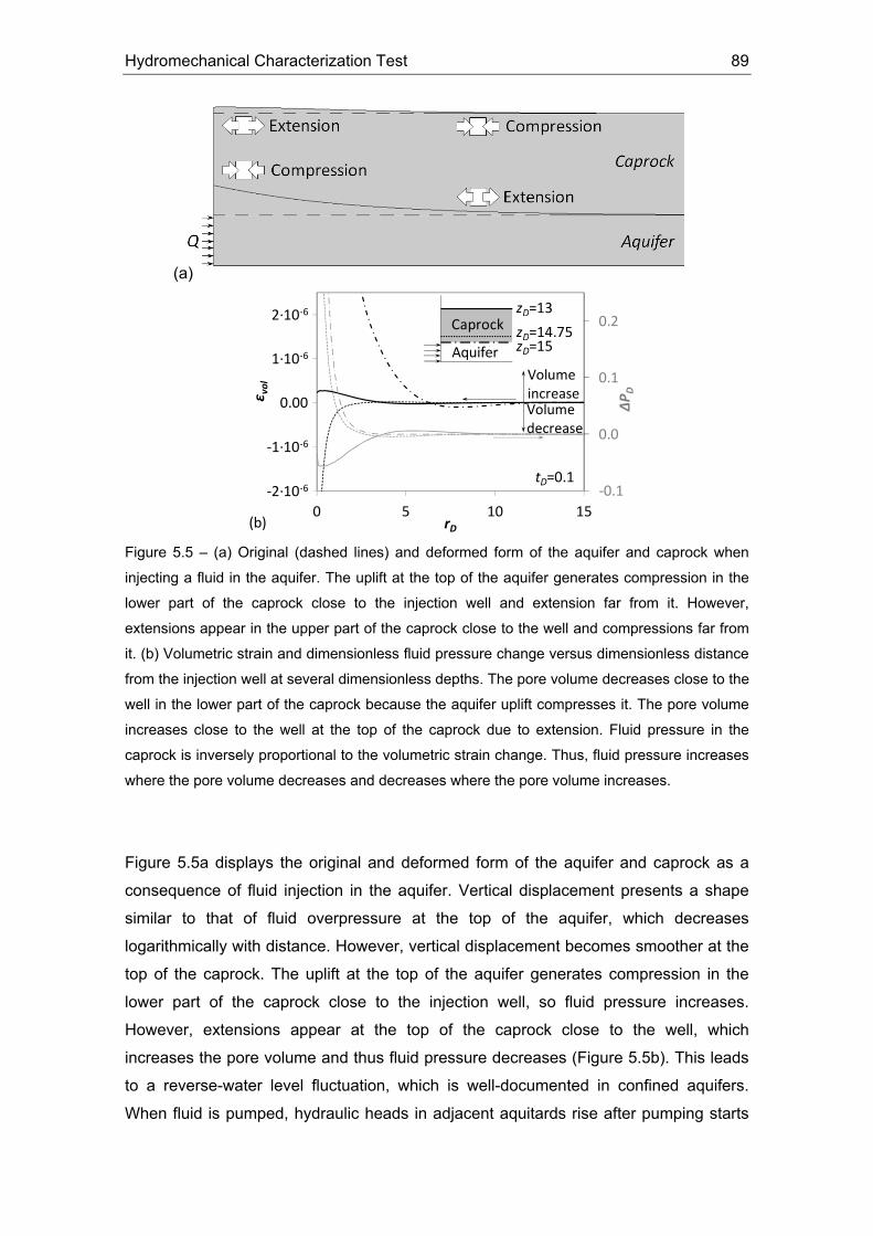
Hydromechanical Characterization Test 89
‐0.1
0.0
0.1
0.2
0.00
0.00
0.00
0.00
0.00
0 5 10 15
ΔPDε vol
rD
Volume increaseVolume decrease
zD=13
zD=15zD=14.75
Caprock
Aquifer
‐2∙10‐6
‐1∙10‐6
1∙10‐6
2∙10‐6
0.00
tD=0.1
(b) Figure 5.5 – (a) Original (dashed lines) and deformed form of the aquifer and caprock when
injecting a fluid in the aquifer. The uplift at the top of the aquifer generates compression in the
lower part of the caprock close to the injection well and extension far from it. However,
extensions appear in the upper part of the caprock close to the well and compressions far from
it. (b) Volumetric strain and dimensionless fluid pressure change versus dimensionless distance
from the injection well at several dimensionless depths. The pore volume decreases close to the
well in the lower part of the caprock because the aquifer uplift compresses it. The pore volume
increases close to the well at the top of the caprock due to extension. Fluid pressure in the
caprock is inversely proportional to the volumetric strain change. Thus, fluid pressure increases
where the pore volume decreases and decreases where the pore volume increases.
Figure 5.5a displays the original and deformed form of the aquifer and caprock as a
consequence of fluid injection in the aquifer. Vertical displacement presents a shape
similar to that of fluid overpressure at the top of the aquifer, which decreases
logarithmically with distance. However, vertical displacement becomes smoother at the
top of the caprock. The uplift at the top of the aquifer generates compression in the
lower part of the caprock close to the injection well, so fluid pressure increases.
However, extensions appear at the top of the caprock close to the well, which
increases the pore volume and thus fluid pressure decreases (Figure 5.5b). This leads
to a reverse-water level fluctuation, which is well-documented in confined aquifers.
When fluid is pumped, hydraulic heads in adjacent aquitards rise after pumping starts
(a)
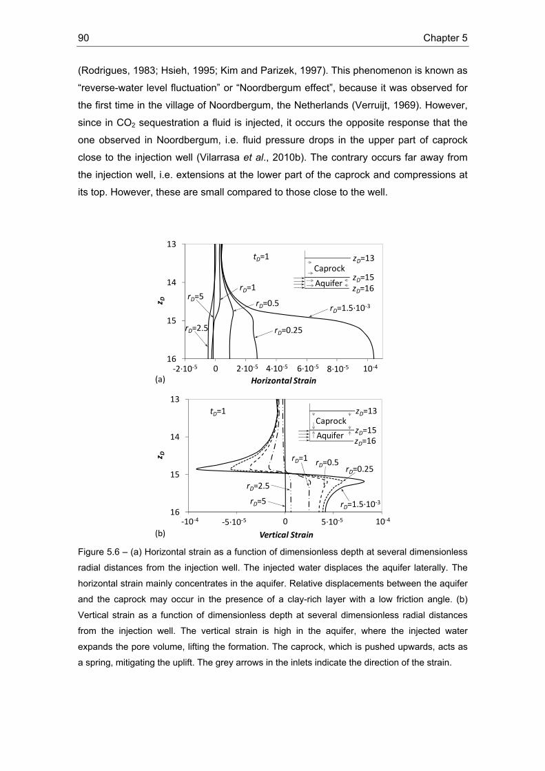
90 Chapter 5
(Rodrigues, 1983; Hsieh, 1995; Kim and Parizek, 1997). This phenomenon is known as
“reverse-water level fluctuation” or “Noordbergum effect”, because it was observed for
the first time in the village of Noordbergum, the Netherlands (Verruijt, 1969). However,
since in CO2 sequestration a fluid is injected, it occurs the opposite response that the
one observed in Noordbergum, i.e. fluid pressure drops in the upper part of caprock
close to the injection well (Vilarrasa et al., 2010b). The contrary occurs far away from
the injection well, i.e. extensions at the lower part of the caprock and compressions at
its top. However, these are small compared to those close to the well.
13
14
15
16‐0.00002 0 0.00002 4E‐05 6E‐05 8E‐05 0.0001
z D
Horizontal Strain
zD=13
zD=15zD=16
Caprock
Aquifer
tD=1
rD=1.5∙10‐3
rD=0.25
rD=0.5
rD=1
rD=2.5
rD=5
(a)‐2∙10‐5 2∙10‐50 6∙10‐5 10‐44∙10‐5 8∙10‐5
13
14
15
16‐0.0001 ‐0.00005 0 5E‐05 0.0001
z D
Vertical Strain
tD=1
rD=0.25rD=0.5
rD=1
rD=2.5
rD=5
zD=15zD=16
Caprock
Aquifer
zD=13
rD=1.5∙10‐3
(b)‐10‐4 ‐5∙10‐5 0 5∙10‐5 10‐4
Figure 5.6 – (a) Horizontal strain as a function of dimensionless depth at several dimensionless
radial distances from the injection well. The injected water displaces the aquifer laterally. The
horizontal strain mainly concentrates in the aquifer. Relative displacements between the aquifer
and the caprock may occur in the presence of a clay-rich layer with a low friction angle. (b)
Vertical strain as a function of dimensionless depth at several dimensionless radial distances
from the injection well. The vertical strain is high in the aquifer, where the injected water
expands the pore volume, lifting the formation. The caprock, which is pushed upwards, acts as
a spring, mitigating the uplift. The grey arrows in the inlets indicate the direction of the strain.

Hydromechanical Characterization Test 91
Fluid injection produces both a vertical and a horizontal displacement of the aquifer.
The aquifer is horizontally displaced away from the injection well (Figure 5.6a) and
pushed upwards (Figure 5.6b). The horizontal strain can even become negative at a
certain distance from the well. The deformation of the aquifer produces deformation of
the caprock, with the condition that displacements are continuous at the aquifer-
caprock interface. The caprock acts as a spring, dissipating the deformation of the
aquifer. Hence, horizontal strain decreases rapidly at the lower part of the caprock
(Figura 5.6a) and vertical strain is negative in the caprock (Figura 5.6b), which means
that its thickness becomes smaller. The high gradient of horizontal strain at the aquifer-
caprock contact suggests that relative displacements between the two formations might
occur in the presence of a clay-rich layer with a low friction angle (see Figure 5.2). If
this occurred, microseismic events would be triggered.
5.4.2. Sensitivity analysis
a) Aquifer
The mechanical properties of the rocks that form the reservoir and the caprock in
potential CO2 storage sites are highly variable (see Section 5.2). We analyze the
sensitivity to the mechanical properties within each geological formation separately. We
start by varying the mechanical properties of the aquifer while maintaining those of the
caprock constant. The ratio of the caprock to aquifer thickness is set to 2.
Figure 5.7 displays the dimensionless overpressure and vertical displacement as a
function of the dimensionless group of the volumetric strain term aqaqaq LeG /13/ +′=Γ
(second term in the left hand side of Eq. (5.22)) at the top of the aquifer and the top of
the caprock. The results correspond to a dimensionless time equal to 1 and a
dimensionless distance from the injection well of 0.5. The most relevant variables in
this analysis are listed in Table 5.1. The dimensionless group of the volumetric strain
term aqΓ is a measure of the stiffness of the rock. High values of aqΓ indicate a stiff
rock and low values of aqΓ indicate a soft rock. Dimensionless fluid overpressure in the
aquifer decreases slightly as the aquifer becomes stiffer and the effect of the Poisson
ratio has little effect (Figure 5.7a). The reverse-water level fluctuation is more
pronounced for soft aquifers, which can lead to a fluid pressure drop at the top of the
caprock almost as high as the overpressure in the aquifer. However, fluid pressure
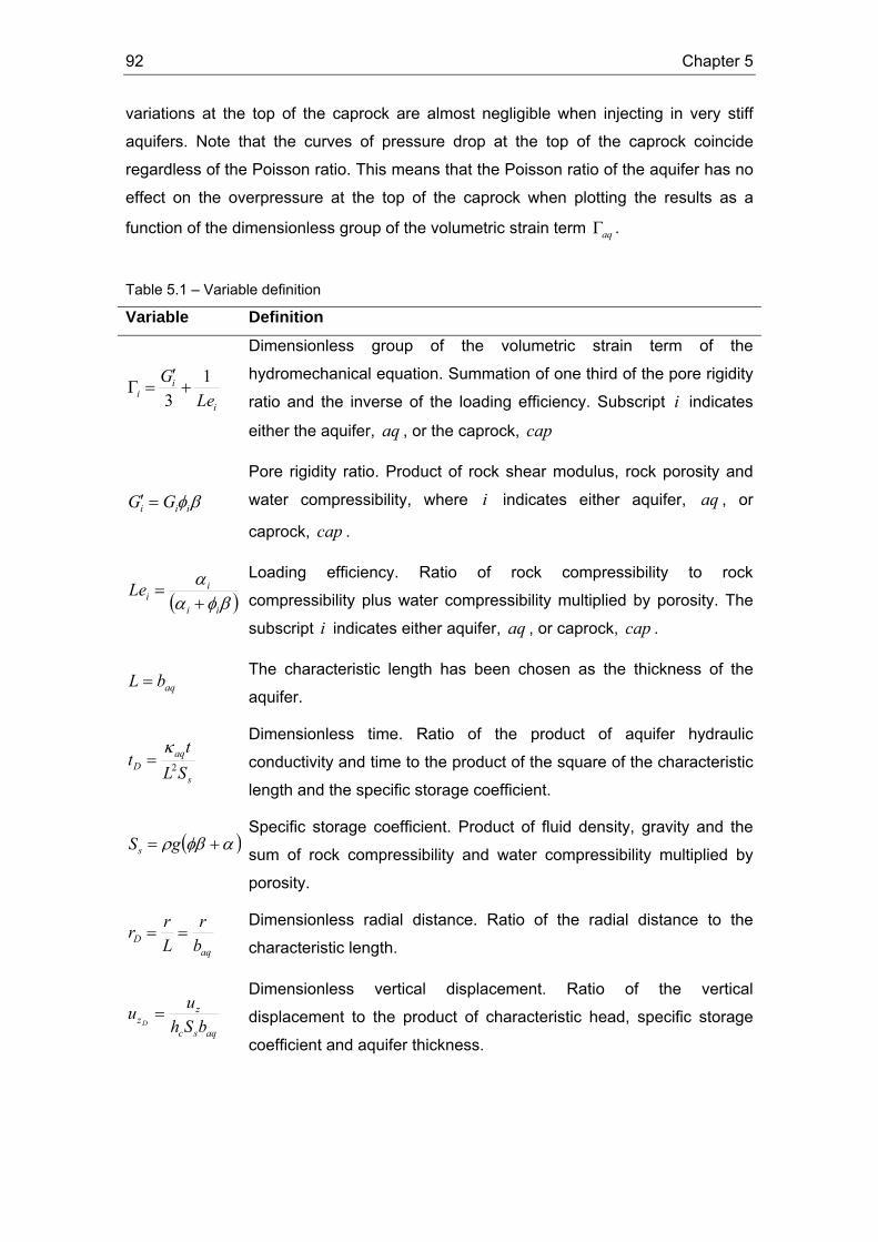
92 Chapter 5
variations at the top of the caprock are almost negligible when injecting in very stiff
aquifers. Note that the curves of pressure drop at the top of the caprock coincide
regardless of the Poisson ratio. This means that the Poisson ratio of the aquifer has no
effect on the overpressure at the top of the caprock when plotting the results as a
function of the dimensionless group of the volumetric strain term aqΓ .
Table 5.1 – Variable definition
Variable Definition
i
ii LeG 13+′
=Γ
Dimensionless group of the volumetric strain term of the
hydromechanical equation. Summation of one third of the pore rigidity
ratio and the inverse of the loading efficiency. Subscript i indicates
either the aquifer, aq , or the caprock, cap
βφiii GG =′
Pore rigidity ratio. Product of rock shear modulus, rock porosity and
water compressibility, where i indicates either aquifer, aq , or
caprock, cap .
( )βφαα
ii
iiLe +=
Loading efficiency. Ratio of rock compressibility to rock
compressibility plus water compressibility multiplied by porosity. The
subscript i indicates either aquifer, aq , or caprock, cap .
aqbL = The characteristic length has been chosen as the thickness of the
aquifer.
s
aqD SL
tt 2
κ=
Dimensionless time. Ratio of the product of aquifer hydraulic
conductivity and time to the product of the square of the characteristic
length and the specific storage coefficient.
( )αφβρ += gSs
Specific storage coefficient. Product of fluid density, gravity and the
sum of rock compressibility and water compressibility multiplied by
porosity.
aqD b
rLrr ==
Dimensionless radial distance. Ratio of the radial distance to the
characteristic length.
aqsc
zz bSh
uuD=
Dimensionless vertical displacement. Ratio of the vertical
displacement to the product of characteristic head, specific storage
coefficient and aquifer thickness.
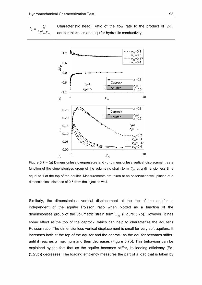
Hydromechanical Characterization Test 93
aqaqc b
Qhκπ2
= Characteristic head. Ratio of the flow rate to the product of π2 ,
aquifer thickness and aquifer hydraulic conductivity.
‐1.2
‐0.6
0.0
0.6
1.2
1 10
ΔPD
Γaq
Aquifer
CaprockzD=15zD=16
zD=13
νaq=0.2 νaq=0.3
νaq=0.4νaq=0.37
tD=1
rD=0.5
(a)
0.00
0.05
0.10
0.15
0.20
0.25
1 10
u zD
Γaq
Aquifer
CaprockzD=15zD=16
zD=13
tD=1rD=0.5
νaq=0.2 νaq=0.3
νaq=0.4νaq=0.37
(b) Figure 5.7 – (a) Dimensionless overpressure and (b) dimensionless vertical displacement as a
function of the dimensionless group of the volumetric strain term aqΓ at a dimensionless time
equal to 1 at the top of the aquifer. Measurements are taken at an observation well placed at a
dimensionless distance of 0.5 from the injection well.
Similarly, the dimensionless vertical displacement at the top of the aquifer is
independent of the aquifer Poisson ratio when plotted as a function of the
dimensionless group of the volumetric strain term aqΓ (Figure 5.7b). However, it has
some effect at the top of the caprock, which can help to characterize the aquifer’s
Poisson ratio. The dimensionless vertical displacement is small for very soft aquifers. It
increases both at the top of the aquifer and the caprock as the aquifer becomes stiffer,
until it reaches a maximum and then decreases (Figure 5.7b). This behaviour can be
explained by the fact that as the aquifer becomes stiffer, its loading efficiency (Eq.
(5.23b)) decreases. The loading efficiency measures the part of a load that is taken by
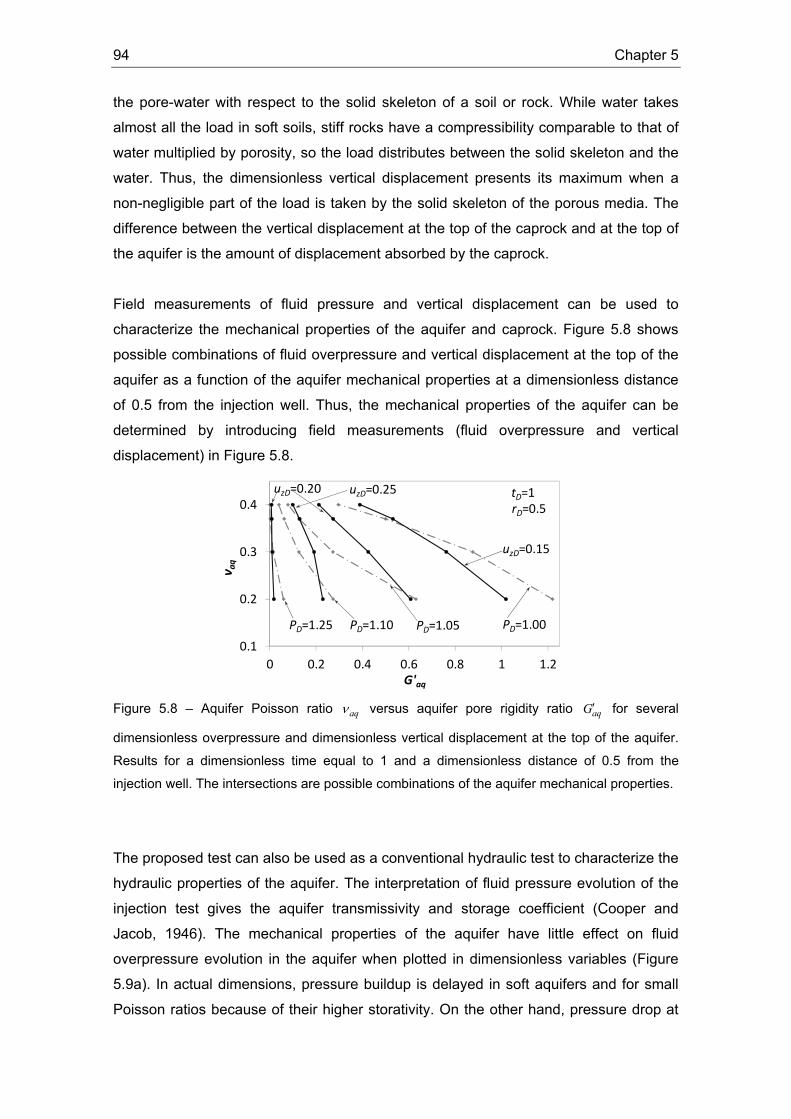
94 Chapter 5
the pore-water with respect to the solid skeleton of a soil or rock. While water takes
almost all the load in soft soils, stiff rocks have a compressibility comparable to that of
water multiplied by porosity, so the load distributes between the solid skeleton and the
water. Thus, the dimensionless vertical displacement presents its maximum when a
non-negligible part of the load is taken by the solid skeleton of the porous media. The
difference between the vertical displacement at the top of the caprock and at the top of
the aquifer is the amount of displacement absorbed by the caprock.
Field measurements of fluid pressure and vertical displacement can be used to
characterize the mechanical properties of the aquifer and caprock. Figure 5.8 shows
possible combinations of fluid overpressure and vertical displacement at the top of the
aquifer as a function of the aquifer mechanical properties at a dimensionless distance
of 0.5 from the injection well. Thus, the mechanical properties of the aquifer can be
determined by introducing field measurements (fluid overpressure and vertical
displacement) in Figure 5.8.
0.1
0.2
0.3
0.4
0 0.2 0.4 0.6 0.8 1 1.2
ν aq
G'aq
PD=1.00
tD=1
uzD=0.15
rD=0.5
uzD=0.20 uzD=0.25
PD=1.05PD=1.10PD=1.25
Figure 5.8 – Aquifer Poisson ratio aqν versus aquifer pore rigidity ratio aqG′ for several
dimensionless overpressure and dimensionless vertical displacement at the top of the aquifer.
Results for a dimensionless time equal to 1 and a dimensionless distance of 0.5 from the
injection well. The intersections are possible combinations of the aquifer mechanical properties.
The proposed test can also be used as a conventional hydraulic test to characterize the
hydraulic properties of the aquifer. The interpretation of fluid pressure evolution of the
injection test gives the aquifer transmissivity and storage coefficient (Cooper and
Jacob, 1946). The mechanical properties of the aquifer have little effect on fluid
overpressure evolution in the aquifer when plotted in dimensionless variables (Figure
5.9a). In actual dimensions, pressure buildup is delayed in soft aquifers and for small
Poisson ratios because of their higher storativity. On the other hand, pressure drop at
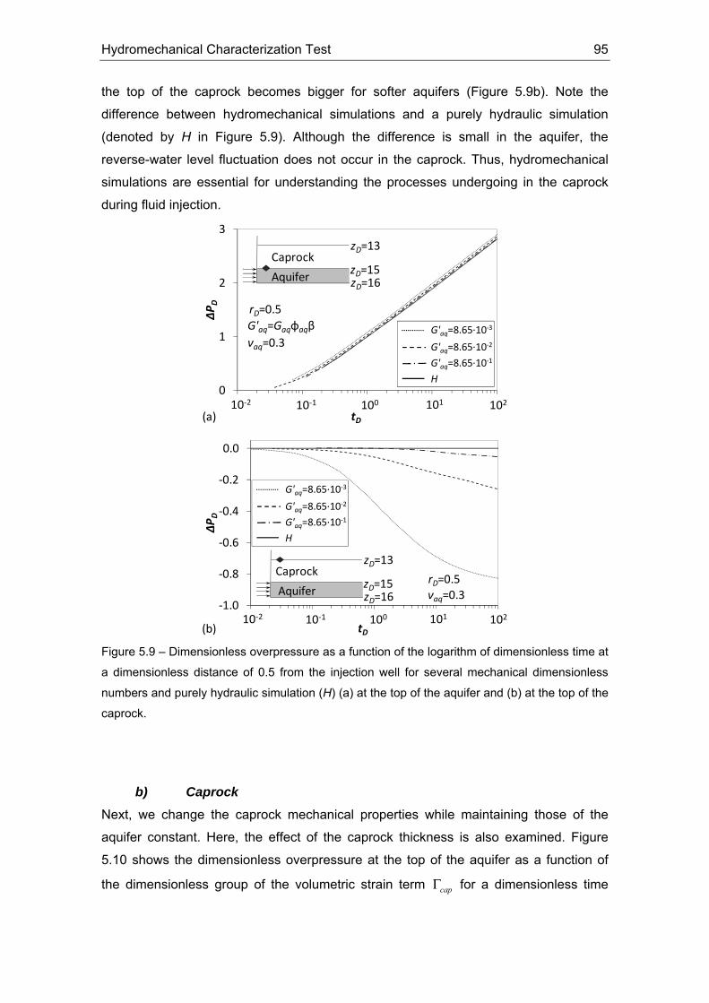
Hydromechanical Characterization Test 95
the top of the caprock becomes bigger for softer aquifers (Figure 5.9b). Note the
difference between hydromechanical simulations and a purely hydraulic simulation
(denoted by H in Figure 5.9). Although the difference is small in the aquifer, the
reverse-water level fluctuation does not occur in the caprock. Thus, hydromechanical
simulations are essential for understanding the processes undergoing in the caprock
during fluid injection.
0
1
2
3
0.01 0.1 1 10 100
ΔPD
tD
G'aq=8.65∙10‐3
G'aq=8.65∙10‐2
G'aq=8.65∙10‐1
H
rD=0.5G'aq=Gaqφaqβνaq=0.3
Aquifer
CaprockzD=15zD=16
zD=13
10‐1 100 101 10210‐2(a)
‐1.0
‐0.8
‐0.6
‐0.4
‐0.2
0.0
0.01 0.1 1 10 100
ΔPD
tD
G'aq=8.65∙10‐3
G'aq=8.65∙10‐2
G'aq=8.65∙10‐1
H
rD=0.5νaq=0.3Aquifer
CaprockzD=15zD=16
zD=13
10‐2 10‐1 100 101 102(b)
Figure 5.9 – Dimensionless overpressure as a function of the logarithm of dimensionless time at
a dimensionless distance of 0.5 from the injection well for several mechanical dimensionless
numbers and purely hydraulic simulation (H) (a) at the top of the aquifer and (b) at the top of the
caprock.
b) Caprock
Next, we change the caprock mechanical properties while maintaining those of the
aquifer constant. Here, the effect of the caprock thickness is also examined. Figure
5.10 shows the dimensionless overpressure at the top of the aquifer as a function of
the dimensionless group of the volumetric strain term capΓ for a dimensionless time
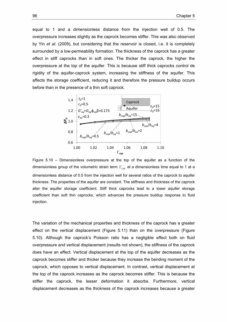
96 Chapter 5
equal to 1 and a dimensionless distance from the injection well of 0.5. The
overpressure increases slightly as the caprock becomes stiffer. This was also observed
by Yin et al. (2009), but considering that the reservoir is closed, i.e. it is completely
surrounded by a low-permeability formation. The thickness of the caprock has a greater
effect in stiff caprocks than in soft ones. The thicker the caprock, the higher the
overpressure at the top of the aquifer. This is because stiff thick caprocks control de
rigidity of the aquifer-caprock system, increasing the stiffness of the aquifer. This
affects the storage coefficient, reducing it and therefore the pressure buildup occurs
before than in the presence of a thin soft caprock.
0.6
0.8
1.0
1.2
1.4
1.00 1.02 1.04 1.06 1.08 1.10
ΔPD
Γcap
G'aq=Gaqφaqβ=0.173
νaq=0.3
bcap/baq=1bcap/baq=2
bcap/baq=0.5
tD=1
bcap/baq=15
rD=0.5Aquifer
CaprockzD=15zD=16
bcap/baq=4
Figure 5.10 – Dimensionless overpressure at the top of the aquifer as a function of the
dimensionless group of the volumetric strain term capΓ at a dimensionless time equal to 1 at a
dimensionless distance of 0.5 from the injection well for several ratios of the caprock to aquifer
thickness. The properties of the aquifer are constant. The stiffness and thickness of the caprock
alter the aquifer storage coefficient. Stiff thick caprocks lead to a lower aquifer storage
coefficient than soft thin caprocks, which advances the pressure buildup response to fluid
injection.
The variation of the mechanical properties and thickness of the caprock has a greater
effect on the vertical displacement (Figure 5.11) than on the overpressure (Figure
5.10). Although the caprock’s Poisson ratio has a negligible effect both on fluid
overpressure and vertical displacement (results not shown), the stiffness of the caprock
does have an effect. Vertical displacement at the top of the aquifer decreases as the
caprock becomes stiffer and thicker because they increase the bending moment of the
caprock, which opposes to vertical displacement. In contrast, vertical displacement at
the top of the caprock increases as the caprock becomes stiffer. This is because the
stiffer the caprock, the lesser deformation it absorbs. Furthermore, vertical
displacement decreases as the thickness of the caprock increases because a greater

Hydromechanical Characterization Test 97
deformation can be absorbed within the caprock. This leads to the extreme case of
thick soft caprocks that can yield subsidence at the top of the caprock (Figure 5.11).
The dashed lines reproduce the vertical displacement of a caprock that reaches the
surface at the depths of the top of all the considered caprocks. The vertical
displacement is similar at all depths when the caprocks are soft. However, the
deformation within the caprock is significantly different for stiff caprocks, in part
because the vertical displacement at the top of the aquifer is controlled by the caprock
thickness.
‐0.1
0.0
0.1
0.2
0.3
1.00 1.02 1.04 1.06 1.08 1.10
u zD
Гcap
bcap/baq=4
bcap/baq=0.5
bcap/baq=2bcap/baq=1
bcap/baq=15
AquiferCaprock
zD=15zD=16
tD=1rD=0.5
G'aq=Gaqφaqβ=0.173νaq=0.3
Figure 5.11 – Dimensionless vertical displacement at the top of the aquifer and the caprock as a
function of the dimensionless group of the volumetric strain term capΓ at a dimensionless time
equal to 1 at a dimensionless distance of 0.5 from the injection well for several ratios of the
caprock to aquifer thickness. The properties of the aquifer are constant. Thick caprocks with
low-rigidity can yield subsidence.
5.4.3. Induced microseismicity analysis
a) Elastic models
Figure 5.12 displays the mobilized friction angle at the top of both the aquifer and the
caprock as a function of the dip angle of a pre-existing cohesionless fracture for a
dimensionless time equal to 1. The vertical stress is the maximum principal stress and
the horizontal stresses are equal due to axysimmetry in this slip tendency analysis. Soft
aquifers yield a higher mobilized friction angle than stiff aquifers. However, the stiffness
of the aquifer has little effect on the mobilized friction angle. On the other hand, the
stiffness of the caprock has a negligible effect on the mobilized friction angle. The
maximum mobilized friction angles at the top of the aquifer are in the order of 25-30°
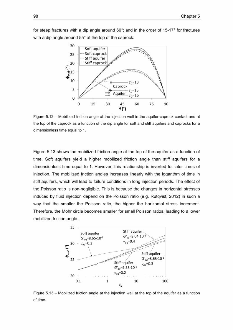
98 Chapter 5
for steep fractures with a dip angle around 60°; and in the order of 15-17° for fractures
with a dip angle around 55° at the top of the caprock.
0
5
10
15
20
25
30
0 15 30 45 60 75 90
φmob(°)
θ (°)
Stiff caprockStiff aquiferSoft caprockSoft aquifer
Aquifer
CaprockzD=15zD=16
zD=13
Figure 5.12 – Mobilized friction angle at the injection well in the aquifer-caprock contact and at
the top of the caprock as a function of the dip angle for soft and stiff aquifers and caprocks for a
dimensionless time equal to 1.
Figure 5.13 shows the mobilized friction angle at the top of the aquifer as a function of
time. Soft aquifers yield a higher mobilized friction angle than stiff aquifers for a
dimensionless time equal to 1. However, this relationship is inverted for later times of
injection. The mobilized friction angles increases linearly with the logarithm of time in
stiff aquifers, which will lead to failure conditions in long injection periods. The effect of
the Poisson ratio is non-negligible. This is because the changes in horizontal stresses
induced by fluid injection depend on the Poisson ratio (e.g. Rutqvist, 2012) in such a
way that the smaller the Poisson ratio, the higher the horizontal stress increment.
Therefore, the Mohr circle becomes smaller for small Poisson ratios, leading to a lower
mobilized friction angle.
20
25
30
35
0.1 1 10 100
φmob(°)
tD
Stiff aquiferG'aq=8.65∙10‐1
νaq=0.3
Stiff aquiferG'aq=8.04∙10‐1
νaq=0.4
Stiff aquiferG'aq=9.38∙10‐1
νaq=0.2
Soft aquiferG'aq=8.65∙10‐3
νaq=0.3
Figure 5.13 – Mobilized friction angle at the injection well at the top of the aquifer as a function
of time.
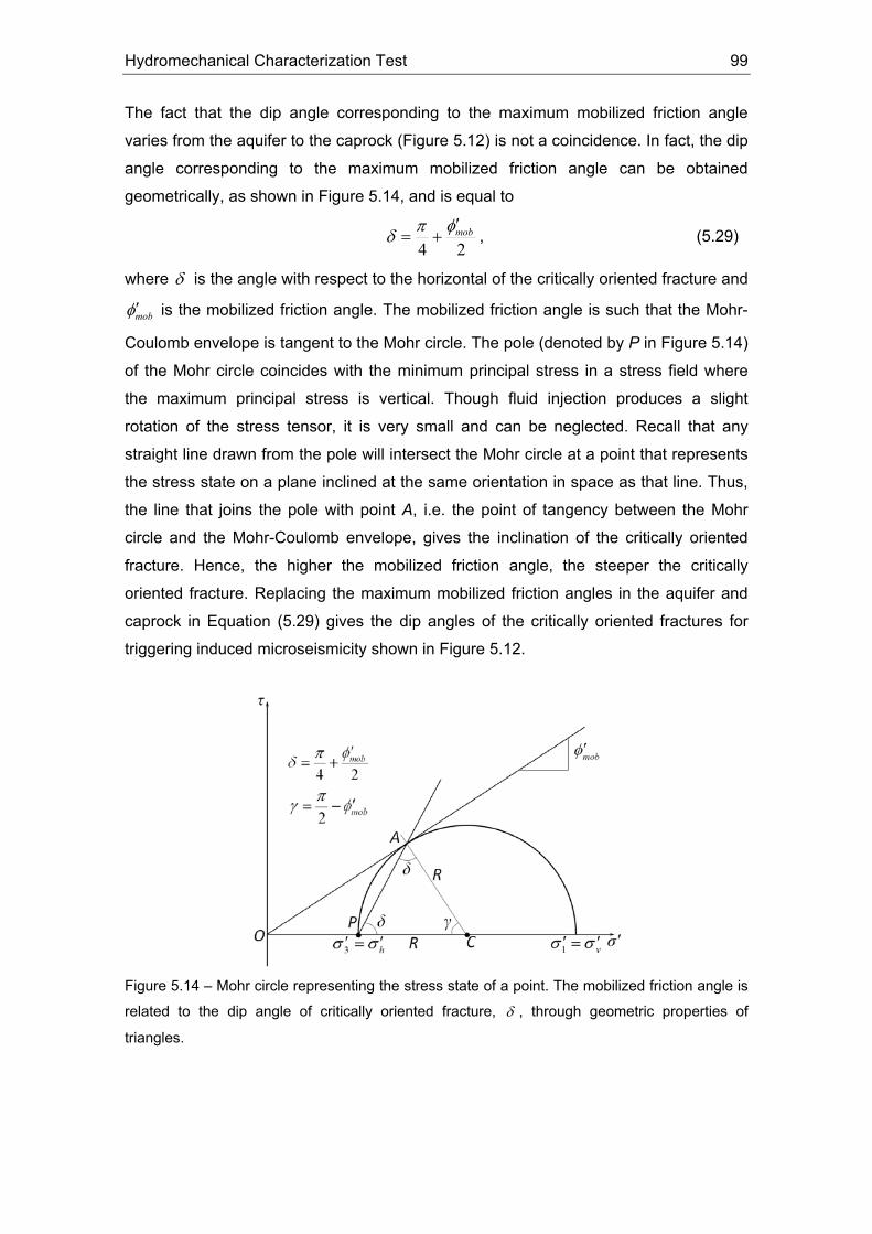
Hydromechanical Characterization Test 99
The fact that the dip angle corresponding to the maximum mobilized friction angle
varies from the aquifer to the caprock (Figure 5.12) is not a coincidence. In fact, the dip
angle corresponding to the maximum mobilized friction angle can be obtained
geometrically, as shown in Figure 5.14, and is equal to
24mobφπδ′
+= , (5.29)
where δ is the angle with respect to the horizontal of the critically oriented fracture and
mobφ′ is the mobilized friction angle. The mobilized friction angle is such that the Mohr-
Coulomb envelope is tangent to the Mohr circle. The pole (denoted by P in Figure 5.14)
of the Mohr circle coincides with the minimum principal stress in a stress field where
the maximum principal stress is vertical. Though fluid injection produces a slight
rotation of the stress tensor, it is very small and can be neglected. Recall that any
straight line drawn from the pole will intersect the Mohr circle at a point that represents
the stress state on a plane inclined at the same orientation in space as that line. Thus,
the line that joins the pole with point A, i.e. the point of tangency between the Mohr
circle and the Mohr-Coulomb envelope, gives the inclination of the critically oriented
fracture. Hence, the higher the mobilized friction angle, the steeper the critically
oriented fracture. Replacing the maximum mobilized friction angles in the aquifer and
caprock in Equation (5.29) gives the dip angles of the critically oriented fractures for
triggering induced microseismicity shown in Figure 5.12.
Figure 5.14 – Mohr circle representing the stress state of a point. The mobilized friction angle is
related to the dip angle of critically oriented fracture, δ , through geometric properties of
triangles.

100 Chapter 5
b) Plastic models
The type of faulting is determined by the stress tensor. In a normal faulting stress
regime, rock fails along steep shear planes (Figure 5.15b, c). The numerical model
reproduces very well the plastic propagation, which follows an angle equal to
2/4/ φπ ′+ (Figure 5.15c). Note that this is the same stress regime as the one
analysed in the previous section. The fact that the rock has some cohesion does not
affect the angle in which shear occurs because the proportions between the triangles in
the Mohr-Coulomb failure analysis are maintained (Figure 5.15a).
Figure 5.15 – Normal faulting stress regime. (a) Mohr circle at failure, (b) schematic
representation of the failure mechanism and (c) plastic deformation obtained from a numerical
simulation.
In a strike slip stress regime, vertical shear planes are formed (Figure 5.16b). The
situation of the pole is somewhat arbitrary in this stress regime. The pole coincides with
the maximum horizontal principal effective stress in Figure 5.16a. However, if the pole

Hydromechanical Characterization Test 101
had coincided with the minimum horizontal principal effective stress, the angle with
respect to this direction in which shear occurs would have been the complimentary of
the one shown in Figure 5.16a, i.e., 2/4/ φπ ′+ , leading to the same orientation of the
shear plane shown in Figure 5.16b. Numerical results show that plastic deformation is
vertical and perpendicular to the maximum horizontal stress (Figure 5.16c). The region
that presents plastic deformations is relatively wide because viscoplasticity regularizes
and does not localize the failure mechanism.
Figure 5.16 – Strike slip faulting stress regime. (a) Mohr circle at failure, (b) schematic
representation of the failure mechanism and (c) plastic deformation obtained from a numerical
simulation.
In a reverse faulting stress regime, rock fails along shallowly dipping shear planes
(Figure 5.17b, c). In this case, the pole coincides with the maximum horizontal principal
effective stress and thus the failure plane (line P-A) presents a dip angle equal to
2/4/ φπ ′− , which is lower than 45º (Figure 5.17a). Figure 5.17c shows plastic
deformations occurring subhorizontally. Microseismicity monitoring can give a clue of

102 Chapter 5
the existing stress tensor at the site by identifying the propagation pattern with one of
these types of faulting.
Figure 5.17 – Reverse faulting stress regime. (a) Mohr circle at failure, (b) schematic
representation of the failure mechanism and (c) plastic deformation obtained from a numerical
simulation.
Figure 5.18 displays deviatoric versus mean effective stresses trajectories of the three
stress regimes at a point of the caprock placed 25 m away from the top of the injection
well in all directions. All the trajectories start inside the failure envelope (elastic
behaviour). However, the trajectories shift to the left because of fluid pressure increase
once fluid injection starts. Finally, all trajectories touch the failure envelope, meaning
that the caprock yields and microseismic events occur.
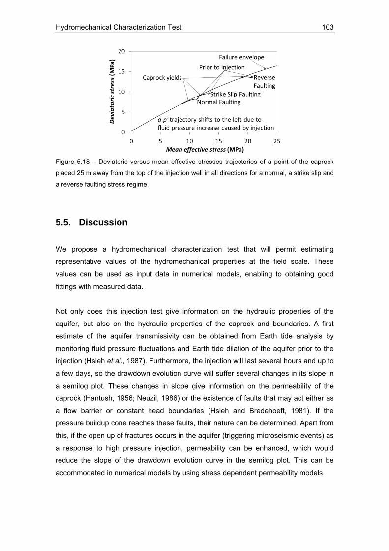
Hydromechanical Characterization Test 103
0
5
10
15
20
0 5 10 15 20 25
Deviatoric stress (M
Pa)
Mean effective stress (MPa)
Caprock yields
q‐p' trajectory shifts to the left due to fluid pressure increase caused by injection
Failure envelope
Reverse Faulting
Strike Slip FaultingNormal Faulting
Prior to injection
Figure 5.18 – Deviatoric versus mean effective stresses trajectories of a point of the caprock
placed 25 m away from the top of the injection well in all directions for a normal, a strike slip and
a reverse faulting stress regime.
5.5. Discussion
We propose a hydromechanical characterization test that will permit estimating
representative values of the hydromechanical properties at the field scale. These
values can be used as input data in numerical models, enabling to obtaining good
fittings with measured data.
Not only does this injection test give information on the hydraulic properties of the
aquifer, but also on the hydraulic properties of the caprock and boundaries. A first
estimate of the aquifer transmissivity can be obtained from Earth tide analysis by
monitoring fluid pressure fluctuations and Earth tide dilation of the aquifer prior to the
injection (Hsieh et al., 1987). Furthermore, the injection will last several hours and up to
a few days, so the drawdown evolution curve will suffer several changes in its slope in
a semilog plot. These changes in slope give information on the permeability of the
caprock (Hantush, 1956; Neuzil, 1986) or the existence of faults that may act either as
a flow barrier or constant head boundaries (Hsieh and Bredehoeft, 1981). If the
pressure buildup cone reaches these faults, their nature can be determined. Apart from
this, if the open up of fractures occurs in the aquifer (triggering microseismic events) as
a response to high pressure injection, permeability can be enhanced, which would
reduce the slope of the drawdown evolution curve in the semilog plot. This can be
accommodated in numerical models by using stress dependent permeability models.
104 Chapter 5
Additionally, this field test can be used as a means of measuring the caprock stability to
fluid injection at high pressure. We suggest injecting water, but CO2 can be used as
well, because it has been observed that water and CO2 have a similar effect on fracture
stimulation (Verdon et al., 2010). Microseismicity monitoring should allow to the
location of the induced microseismic events (Xuan and Sava, 2010). The minimum
detectable magnitude depends on the depth at which an array of geophones can be
placed. Small events, of magnitude ranging from -3 to -2, can be detected only if the
geophones are placed in a nearby borehole at a similar depth than the aquifer-caprock
system (Moeck et al., 2009; Bohnhoff et al., 2010). The fracture slip likelihood as a
function of fracture orientation can be determined from a slip tendency analysis (Segall
and Fitzgerald, 1998; Moeck and Backers, 2011). The mobilized friction angle is higher
in the aquifer than in the caprock (Figure 5.12) because the overpressure induced by
injection translates the Mohr circle to the left (recall Figure 5.4). However, the likelihood
of microseismic events occurrence depends on the actual friction angle of each
formation. For instance, shear failure can occur in the caprock in critically oriented
fractures with low-friction angles (Figure 5.2). The onset of microseismicity in the
caprock can be used to define the maximum sustainable injection pressure. The value
of this sustainable pressure will be a measure of the suitability of a specific site for
permanent CO2 storage. Low values of the maximum sustainable injection pressure are
indicative that the site can undergo large plastic deformations and may reactivate faults
(Rutqvist et al., 2008) through which CO2 could migrate towards freshwater aquifers or
even the surface.
The stress tensor plays an important role in assessing the suitability of a specific site
for permanent CO2 storage. Shear planes are subhorizontal in reverse faulting stress
regime, but they are subvertical in normal faulting stress regime, as shown theoretically
and numerically (Figures 5.15 and 5.17). Thus, it is more likely that the CO2 finds a
migration path that crosses the whole caprock in a normal faulting than in a reverse
faulting stress regime. But, strike slip stress regime seems even more unfavorable,
because shear planes are vertical (Figures 5.16). However, the size of earthquakes
depends on the stress regime. Schorlemmer et al. (2005) found that the largest
earthquakes occur in reverse faulting stress regime; normal faulting stress regime
presents a larger proportion of small earthquakes and strike slip faulting stress regime
has an intermediate behaviour. Hence, the propensity for larger earthquakes in a
reverse faulting stress regime counterbalances the less unfavorable orientation of
shear planes. However, the stress regime should not be a limiting factor if a careful

Hydromechanical Characterization Test 105
monitoring of the hydromechanical response is performed, as evidenced in In Salah
(Rutqvist, 2012), where a strike slip stress regime exists.
The stress tensor can be determined from observation of breakouts, tensile fractures
and induced hydrofractures in wells (Zoback et al., 2003). Alternatively, the observation
of similar patterns in microseismic events (e.g. doublets, multiplets, wavelength, slip
direction) can give clues to determine the stress tensor (Rubin et al., 1999; Tezuka and
Niitsuma, 2000; Pytharouli et al., 2011). The stress tensor determination is not easy
and may change with depth (Plenefisch and Bonjer, 1997; Klee et al., 2011).
Nevertheless, the magnitude and orientation of the principal stresses should be, at
least, delimited in order to have some confidence on the existing stress tensor and how
far or close it is from failure. The latter can be assessed by the interpretation of the
proposed hydromechanical characterization test.
The dimensional analysis of the hydromechanical equations shows that the problem is
governed by two parameters: the loading efficiency and another that we have called
the pore rigidity ratio. However, the later can be expressed as a function of the loading
efficiency and the Poisson ratio as
( )( )ν
ν+−
⎟⎠⎞
⎜⎝⎛ −=′
1221311
LeG . (5.30)
Note that the ratio where the Poisson ratio appears is the shear to bulk modulus ratio,
i.e. KG / . The dimensionless curves of fluid pressure and vertical displacement as a
function of these parameters permit the estimation of the mechanical properties of the
aquifer and caprock. The dimensional analysis considers the possibility that the rock
presents dilatancy. Its effect should be considered as a possible contributing term
when analyzing hydromechanical measurements. Though real potential storage sites
will present a complex geometry, each site may be idealized as one similar to the ones
studied here. Thus, the results presented here will permit to gain insight on the relevant
hydromechanical processes occurring in each site.
One of the more interesting hydromechanical processes occurring during fluid injection
in an aquifer overlaid by a caprock is the reverse-water level fluctuation. These can
only be observed numerically if hydromechanical coupled simulations are performed
(see Figure 5.9). We use this effect, which is more pronounced in soft aquifers, to
determine the geomechanical properties of the rocks. This effect can be difficult to
measure in situ if the aquifer is stiff because it will lead to small fluid pressure changes,
which will only be detectable if the measuring equipment is very accurate.
106 Chapter 5
Vertical displacement is not easy to measure in deep boreholes. Strain measurements
with fiber optic may be an alternative. However, it cannot be said for sure what
deformation is being measured. Is it measuring the strain of the rock? Or is it
measuring that of the casing? The measuring equipment will be embedded in the
cement between the casing and the rock, which are of different stiffness, and thus
deform differently. If the cement-rock contact becomes a sliding surface, then the
measuring equipment will measure the casing strain. This would give the impression
that the rock is much stiffer than it actually is. However, the combined interpretation of
fluid pressure and vertical displacement measurements will help in deciding whether
some measurements are or not representative of the aquifer or caprock. Overall, the
hydromechanical parameters of the aquifer and caprock at the field scale can be
estimated from the interpretation of the proposed hydromechanical characterization
field test.
5.6. Conclusion
We propose a hydromechanical characterization test for determining the aquifer and
caprock hydromechanical properties at the field scale. Additionally, the maximum
sustainable CO2 injection pressure can be determined by monitoring induced
microseismicity. This will help to assess the suitability of specific sites for permanent
CO2 storage in deep saline formations.
We obtain the parameters that govern the problem through a dimensional analysis. We
present the dimensionless overpressure and vertical displacement as a function of
these parameters, which yields a family of curves for several Poisson ratio. Except for
the vertical displacement at the top of the caprock, which depends on the Poisson ratio,
all the curves collapse in one single curve when plotting the results as a function of the
dimensionless group of the volumetric strain term aqΓ . Not only do these curves show
the behaviour of the aquifer-caprock system when injecting a fluid, but also can they be
used for parameter estimation from field measurements.
The coupled hydromechanical simulations of fluid injection show a reverse-water level
fluctuation in the caprock, i.e. fluid pressure drops in the caprock when injecting in the
subjacent aquifer. This phenomenon cannot be observed when running purely

Hydromechanical Characterization Test 107
hydraulic simulations. Thus, coupled hydromechanical simulations should be
performed when the processes that the caprock undergoes during fluid injection are of
interest.
Induced microseismic events are of concern when occurring in the caprock. Although
the mobilized friction angle is lower in the caprock than in the aquifer, rich-clay
materials, like the ones that form the caprock, present low-friction angles, especially in
the direction parallel to bedding. Thus, monitoring microseismicity can give confidence
on the caprock integrity.


109
6. Liquid CO2 Injection for Geological
Storage in Deep Saline Aquifers
6.1. Introduction
Pressure ( p ) and temperature (T ) conditions of deep geological formations suitable
for storing CO2 are such that this greenhouse gas remains in supercritical (SC) state,
i.e. p >7.382 MPa and T >31.04 ºC (e.g. Bachu, 2003). Thus, it is usually assumed
that CO2 will reach the aquifer in SC conditions (e.g. Pruess and Garcia, 2002).
However, injecting CO2 in SC state may not be the best option. Several engineering
methodologies have been proposed as alternatives to the concept of injecting SC CO2.
They focus on accelerating CO2 dissolution to minimize the risk of leakage of free-
phase mobile CO2 by means of dissolving CO2 at surface (Burton and Bryant, 2009;
Jain and Bryant, 2011; Zendehboudi et al., 2011) or at depth (Carrera et al., 2011b), by
injecting brine at some distance from the CO2 injection well that mixes with the CO2
plume enhancing dissolution (Hassanzadeh et al., 2009) or by injecting CO2 under
temporal pressure fluctuations, which enhances CO2 dissolution (Bolster et al., 2009b).
On the other hand, a few studies suggest that cold CO2 (and therefore in liquid state)
injection may have some advantageous implications for CO2 storage (Rayward-Smith
and Woods, 2011; Silva et al., 2011). However, these studies are approximations that
do not take into account the whole coupling of the thermo-hydro-mechanical effects
inherent to cold CO2 injection.
It can be conjectured that injecting CO2 in liquid state is energetically more efficient
than doing so in SC state and more optimal from a storage engineering point of view
because liquid CO2 is denser than SC CO2. Therefore, for a given mass of CO2, a
smaller volume of formation fluid will be displaced, leading to a lower overpressure in
the reservoir. More importantly, the increased weight of liquid CO2 in the injection well
implies that a far lower pressure is required at the wellhead. Additionally, CO2 is usually
transported in liquid state (pressure above 8.5 MPa and ambient temperatures (Figure
6.1)) (McCoy and Rubin, 2008). Thus, it can be injected at the conditions in which it
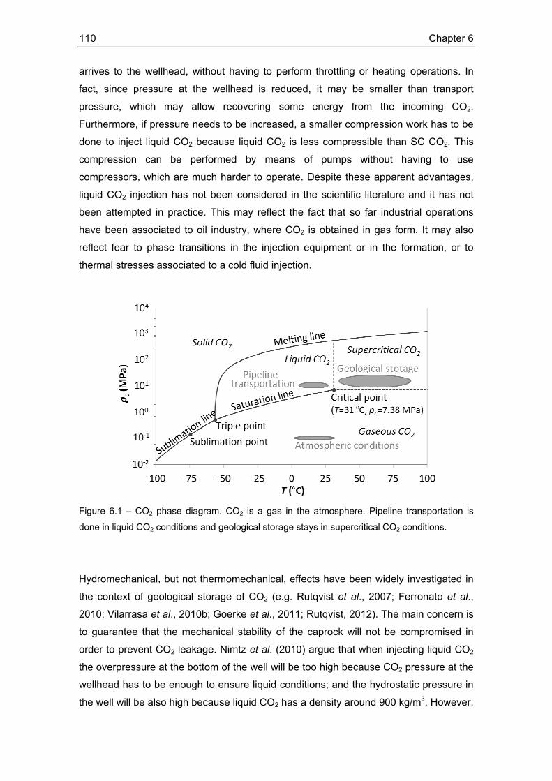
110 Chapter 6
arrives to the wellhead, without having to perform throttling or heating operations. In
fact, since pressure at the wellhead is reduced, it may be smaller than transport
pressure, which may allow recovering some energy from the incoming CO2.
Furthermore, if pressure needs to be increased, a smaller compression work has to be
done to inject liquid CO2 because liquid CO2 is less compressible than SC CO2. This
compression can be performed by means of pumps without having to use
compressors, which are much harder to operate. Despite these apparent advantages,
liquid CO2 injection has not been considered in the scientific literature and it has not
been attempted in practice. This may reflect the fact that so far industrial operations
have been associated to oil industry, where CO2 is obtained in gas form. It may also
reflect fear to phase transitions in the injection equipment or in the formation, or to
thermal stresses associated to a cold fluid injection.
Figure 6.1 – CO2 phase diagram. CO2 is a gas in the atmosphere. Pipeline transportation is
done in liquid CO2 conditions and geological storage stays in supercritical CO2 conditions.
Hydromechanical, but not thermomechanical, effects have been widely investigated in
the context of geological storage of CO2 (e.g. Rutqvist et al., 2007; Ferronato et al.,
2010; Vilarrasa et al., 2010b; Goerke et al., 2011; Rutqvist, 2012). The main concern is
to guarantee that the mechanical stability of the caprock will not be compromised in
order to prevent CO2 leakage. Nimtz et al. (2010) argue that when injecting liquid CO2
the overpressure at the bottom of the well will be too high because CO2 pressure at the
wellhead has to be enough to ensure liquid conditions; and the hydrostatic pressure in
the well will be also high because liquid CO2 has a density around 900 kg/m3. However,
Liquid CO2 Injection 111
they do not perform any hydromechanical simulation to confirm their hypothesis.
Moreover, they do not consider reducing temperature, which ensures liquid conditions
with moderate pressures. Note that an excessive overpressure can induce
microseismicity (Phillips et al., 2002; Guglielmi et al., 2008; Cappa and Rutqvist,
2011b), which may open up migration paths for CO2. However, since liquid CO2 is
colder than the formations where it will be injected, liquid CO2 injection implies a
combination of hydromechanical and thermomechanical effects that should be studied
simultaneously to properly evaluate the caprock mechanical stability.
The injection of a cold fluid induces a thermal contraction of the rock, leading to a
reduction of the effective stresses (Segall and Fitzgerald, 1998). In general, the smaller
the effective stresses, the closer to failure conditions. Thermomechanical effects have
been studied specially in geothermal reservoir stimulation (Ghassemi et al., 2007;
Majer et al., 2007). In geological storage of CO2, Preisig and Prévost (2011) studied the
thermomechanical effects of injecting CO2 at a colder temperature than that of the
reservoir at In Salah (Algeria), but assuming constant CO2 properties, which may not
be realistic (see Appendix II). On the other hand, non-isothermal CO2 flow simulations
considering the actual CO2 properties have been performed, but without considering
the mechanical coupling and always in supercritical conditions (Han et al., 2010; Singh
et al., 2011). Therefore, the thermomechanical effects of liquid CO2 injection remain to
be studied.
We propose to inject CO2 in liquid state as a new engineering methodology for
minimizing energy costs and CO2 phase changes in the capture-transport-injection
chain, and improving the short- and long-term storage efficiency of CO2. This injection
concept will be tested at the pilot site of Hontomín (Carrera et al., 2011a), Burgos,
Spain, which is the injection site of the CO2 storage Technology Demonstration Plant
(TDP) of the Compostilla OXYCFB300 project (EU funded: European Energy
Programme for Recovery), operated by Fundación Ciudad de la Energía (CIUDEN).
Hontomín is a dome-like structure with a dolomitized reservoir located at 1450 m depth,
which is overlaid by a caprock made of marls. A large number of experiments are
planned both for site characterization and for injection technology development
(Carrera et al., 2011a).
The objective of this chapter is to analyze liquid CO2 injection into a deep aquifer in
terms of (1) the energetic efficiency and (2) caprock mechanical stability. This
represents a first step towards the design of the liquid CO2 injection test that will be
112 Chapter 6
performed at the Hontomín pilot test. We calculate CO2 flow in both an injection well
and a deep saline formation. We perform simulations of non-isothermal two-phase flow
in a deformable porous media to evaluate the caprock mechanical stability.
6.2. Mathematical and numerical methods
We first solve CO2 injection in a vertical injection well and afterwards in a saline
formation. The geometry of the problem consists in a homogeneous 100 m thick
horizontal aquifer that is overlaid and underlain by a seal. The system is axisymmetric
and extends laterally 20 km. The nature of the outer hydraulic boundary condition does
not affect the results because the radius of the pressure perturbation cone is smaller
than the radius of the domain for the injection time scales presented here. Therefore,
the model behaves as an infinitely acting aquifer. The top of the aquifer is located at a
depth of 1500 m, which corresponds to the depth of the reservoir at the Hontomín test
site. The seals that overlay and underlie the aquifer have a thickness of 200 m. The
seal that is placed on top of the aquifer, i.e. the caprock, is covered by a 1300 m thick
low shear strength media that do not need to be included in the model. An injection well
with a radius of 0.15 m is placed in the center of the domain.
6.2.1. Non-isothermal flow in the injection pipe Flow of CO2, or any fluid, and its mixtures in non-isothermal wells involves solving the
partial differential equation (PDE) that express energy, mass and momentum
conservation. These PDEs are coupled through the equations of state (EOS) governing
fluid and thermodynamic properties. Several authors describe numerical procedures to
solve these equations (Lu and Connell, 2008; Paterson et al., 2008; Pan et al., 2009;
Han et al., 2010).
Here, we adopted the approach of Lu and Connell (2008). They presented a
methodology to solve steady state non-isothermal multiphase flow of CO2 in an
injection well, in which the flow equations are based on the averaged-flow model (e.g.
Brill and Mukherjee, 1999; Hasan and Kabir, 2002). We assume that the steady state
assumption describes reasonably well the operation after the initial stages. This leads
to a system of one dimensional ordinary differential equation (ODE) along the vertical
coordinate z . The number of equations of such system is five for single-phase
Liquid CO2 Injection 113
conditions or twelve for two-phase conditions. The corresponding vectors of unknown
state variables are ( )tThpv ,,,,ρ=x or ( )tsatg
satlglgll hhssXThpv ,,,,,,,,,,, ρρθ=x ,
respectively, where ρ is density, v is velocity of the fluid mixture, p is pressure, h is
specific enthalpy, T is temperature, lθ is volumetric liquid content, X is gas mass
fraction and s is entropy. Subscript l and g stand for liquid and gas phases,
respectively; and superscript sat and t refer to saturation conditions and to transpose,
respectively.
Because solubility of gas into water is neglected, this approach is restricted to pure
CO2 or a multi-component gaseous mixture rich in CO2, but not a fluid mixture of water
and gas. As explained by Lu and Connell (2008), the phase equilibrium condition is
checked to identify the state of the fluid at a given point when solving the system of
equations. If more than one root of the EOS exists and the Gibbs equilibrium condition
applies, then the fluid is identified to be in a two-phase coexistence state and the size
of the system is 12. Otherwise, the fluid is in single-phase conditions and the size of
the system is 5. It should be noted that the above model simplifies considerably when
simulating the injection of liquid CO2, because single-phase conditions (liquid and/or
supercritical) prevail along the entire wellbore.
In the approach of Lu and Connell (2008) the fluid in the injection pipe exchanges heat
laterally with its surroundings. The heat exchange term is represented by
( )( )zTTURQ geop −−= ∞π2 , (6.1)
where ∞U is the overall heat transfer coefficient for the injection well comprising the
thermal properties of all the materials from which it is composed (the injection fluid, the
injection pipe wall, the brine in the annulus between injection pipe and the casing wall,
the casing wall and the cement), pR is the radius of the injection pipe and ( )zTgeo is the
geothermal temperature along the wellbore. We assumed a geothermal gradient of
0.033 ºC/m and a formation temperature at surface of 5 ºC in all the simulations. The
internal diameter of the injection pipe is set at 9 and 15.24 cm. The bottom of the
injection pipe is located at 1500 m, coinciding with the top of the aquifer for CO2
storage.
To solve the system of flow equations, we need to specify 3 boundary conditions
related to the primary physical quantities p , T and v . Additionally, the gas mass
114 Chapter 6
fraction X or the volumetric liquid content lθ need to be specified if injecting two-
phase CO2. Common operational conditions of an injection well are specifying the
pressure and/or the flow rate and the temperature at the wellhead. If a pressure-
controlled injection condition is assumed at the wellhead, a boundary condition relating
the flow rate and the reservoir pressure at the bottom of the well can be specified. In
fact, this boundary condition allows to address the coupling between the flow through
the injection well and that in the reservoir. We study flow through the injection well and
flow in the formation separately to explain the processes occurring in each of them in a
clear way. However, we couple them by choosing a pressure and temperature
conditions at the wellhead, such that the resulting pressure and temperature conditions
at the bottom of the well coincide with the boundary conditions of the two-phase flow
simulations in the reservoir.
As far as fluid properties are concerned, density was calculated assuming the Redlich-
Kwong EOS (Redlich and Kwong, 1949) using the parameters proposed for CO2 by
Spycher et al. (2003) (see Appendix II). Viscosity was calculated according to the
correlation of Altunin and Sakhabetdinov (1972) (see Appendix II). The friction factor of
the fluid through the injection pipe was calculated according to the Blasius equation
(Brill and Mukherjee, 1999; Hassan and Kabir, 2002). Turbulent flow regime can be
also calculated using other empirical correlations that include rugosity of the pipe (e.g.,
Colebrook, 1939; Zigrang and Sylvester, 1985).
The steady state non-isothermal multiphase flow governing equations in the injection
pipe were programmed in MatLab (Silva et al., 2011). These equations are solved
using a variable order method for solving stiff differential equations.
6.2.2. Non-isothermal two-phase flow in a deformable porous media Consider CO2 injection in a deep confined deformable saline formation. In general, the
injected CO2 will not be in thermal equilibrium with the reservoir, especially at high flow
rates (Paterson et al., 2008). To account for these processes, thermo-hydro-
mechanical couplings should be taken into account. Therefore, mass conservation of
each phase, energy balance and momentum balance have to be solved
simultaneously.
Liquid CO2 Injection 115
a) Fluid mass conservation equation
Mass conservation of each phase can be expressed as (Bear 1972),
( ) ( ) wcrtS , , ==⋅∇+∂
∂ αρρϕααα
αα q , (6.2)
where ϕ is porosity, αS is saturation of the α -phase, αρ is density, t is time, αq is
the volumetric flux, αr is the phase change term (i.e. CO2 dissolution into water and
water evaporation into CO2) and α is either CO2 rich phase, c, or aqueous phase, w.
For the sake of simplicity we neglect evaporation of water into CO2, i.e., wr = 0.
Momentum conservation is expressed using Darcy’s law, written as
( ) wczgpkkr , , =∇+∇−= αρμ ααα
ααq , (6.3)
where k is intrinsic permeability, αrk is the α -phase relative permeability, αμ its
viscosity, αp its pressure and g is gravity.
The properties of the aquifer and seals correspond to those of limestone and shale,
respectively (Vilarrasa et al., 2010b) and are detailed in Table 6.1. We consider the
aquifer to be a permeable limestone with homogeneous grain size. Therefore, the entry
pressure is low and the shape parameter of the van Genuchten (1980) retention curve
is high. On the other hand, seal entry pressure is high, which hinders CO2 migration.
Relative permeabilities follow a power law of saturation for both phases: the limestone
has a cubic law, while the power in the seals is 6. CO2 density and viscosity, which are
highly dependent on p and T conditions, are detailed in Appendix II.
Buoyancy effects are relevant in the CO2 plume evolution, regardless of injection
conditions. However, when injecting liquid CO2 the density contrast between CO2 and
brine is smaller than when injecting SC CO2. Additionally, liquid CO2 viscosity is higher
than SC CO2 viscosity. Thus, viscous forces gain strength in front of gravity forces. This
can be quantified through the gravity number (Vilarrasa et al., 2010a)
cm
crcg Q
gbkkrNμ
ρρπ αΔ=2 , (6.4)
where cr is a characteristic length, b is aquifer thickness, ρΔ is the difference
between CO2 and water density and mQ is the CO2 mass flow rate.
116 Chapter 6
Table 6.1 – Material properties used in the thermo-hydro-mechanical analysis of liquid CO2
injection.
Property Aquifer Seal
Permeability, k (m2) 10-13 10-18
Relative water permeability, rwk 3wS 6
wS
Relative CO2 permeability, rck 3cS
6cS
Gas entry pressure, 0p (MPa) 0.02 0.6
van Genuchten, m 0.8 0.5
Porosity, ϕ 0.1 0.01
Young’s modulus, E (GPa) 2.5 5.0
Poisson ratio, ν 0.3 0.3
Thermal conductivity, λ (W/m/K) 1.5 1.5
Thermal expansion coefficient, Tα (ºC-1) 10-5 10-5
b) Energy conservation equation
Energy conservation can be written as (Faust and Mercer, 1979)
( )( ) ( )
( ) 0
1
=++∇−⋅∇
+∂+∂
−∂
++−∂
cccwww
ccwwcccwwwss
hhTt
pSpSt
hShSh
qq ρρλ
ϕϕϕρϕρρϕ, (6.5)
where sρ is solid density, αh is enthalpy of α -phase ( swc ,,=α ; s for solid) and λ
is thermal conductivity.
Eq. (6.5) includes non-isothermal processes, such as Joule-Thomson effect (Tsang et
al., 2008), heat of CO2 dissolution and water evaporation (Han et al., 2010) and
compression work due to the high compressibility of CO2. We consider all these
processes, except water evaporation.
c) Thermoelasticity in porous media
To solve the mechanical problem, the momentum balance of the porous media has to
be satisfied. If inertial terms are neglected, it reduces to the equilibrium of stresses
0bσ =+⋅∇ , (6.6)
where σ is the stress tensor and b is the body forces vector.
Liquid CO2 Injection 117
Furthermore, we assume that the medium behaves elastically. In fact, we use linear
thermoelasticity to acknowledge the effect of changes in fluid pressure and
temperature. Therefore, elastic strain depends on total stress, overpressure and
temperature as (Biot, 1956)
( ) IIIσε TpEEE Tm Δ
−+
−Δ−
−−+
= ανννσνν213
12131 , (6.7)
where ε is the strain tensor, ( ) 3zyxm σσσσ ++= is the mean stress, I is the identity
matrix, E is the Young’s modulus, ν is Poisson ratio and Tα is the linear thermal
expansion coefficient. Here, the sign criterion of geomechanics is adopted, i.e. strain is
positive in compression and negative in extension.
Simulations suggest that the temperature perturbation is localized within a relatively
small volume of the formation close to the injection well, thus acting spherically.
However, the fluid pressure perturbation propagates a long distance in the direction of
the aquifer, but not in the perpendicular, thus acting anisotropically. Therefore, it may
be assumed that stresses vary isotropically with temperature changes and that no
horizontal strain is allowed in the outer boundary as a result of lateral confinement. This
leads to a variation of the vertical and horizontal stresses as a result of fluid pressure
and temperature variations as
( )( )
TEσ Tv Δ−−
=Δ ανν
22131 , (6.8a)
( )( )
TEpσ Th Δ−−
+Δ−−
=Δ ανν
νν
22131
121 , (6.8b)
where vσ is the vertical stress and hσ is the horizontal stress.
Eq. (6.8b) shows that an increase in pore pressure and/or temperature, which
produces an expansion of the porous media, causes an increase of horizontal stresses
because of lateral confinement that opposes to the induced expansion. On the other
hand, a decrease in pressure and/or temperature, which produces a contraction of the
porous media, causes a decrease of horizontal stresses.
d) Model setup
The initial conditions are hydrostatic pressure; temperature following a geothermal
gradient of 0.033 ºC/m, with a surface temperature of 5 ºC; a vertical stress gradient of
0.023 MPa/m and horizontal effective stresses corresponding to a lateral earth
pressure coefficient of either 0.5 (vertical stress higher than horizontal stresses) or 2.0
118 Chapter 6
(horizontal stresses higher than vertical stress). As a first step, a steady-state
calculation is carried out to ensure consistent initial conditions in equilibrium for the
pressure, temperature and stress fields.
The hydraulic boundary conditions are a prescribed CO2 mass flow rate at the injection
well (1.0 Mt/yr) and a constant pressure on the outer boundary. The thermal boundary
conditions are constant temperature at the top and bottom boundaries of the domain.
The thermal perturbation does not reach these boundaries, so the nature of the
boundary condition does not affect the results. The mechanical boundary conditions
are no displacement normal to the bottom, outer and injection well boundaries. A
constant, vertical lithostatic stress is imposed at the top of the caprock.
The mesh is made of structured quadrilateral elements. Laterally, the size of the
elements is of tens of cm close to the injection well and increases exponentially up to a
longitudinal size of 400 m next to the outer boundary. Vertically, the elements within the
aquifer are of 5 m. In the caprock, close to the aquifer-seal contacts the size is of 5 m
and far away from the contact the size grows up to 25 m.
Non-isothermal CO2 injection in a deformable porous media is simulated using the finite
element numerical code CODE_BRIGHT (Olivella et al., 1994, 1996). We have
implemented CO2 properties, such as density, viscosity, enthalpy and heat capacity
(Appendix II) in order to simulate CO2 storage. Furthermore, we have incorporated in
the energy conservation the term of CO2 volumetric compression due to pressure
changes (second term of Eq. (6.5)), maintaining temperature as the state variable.
6.2.3. Mechanical stability To determine whether a pre-existing fracture is stable or not a failure criterion has to be
defined. The medium is stable and behaves elastically while the stress state falls inside
the failure envelope. However, if the stress state touches the failure envelope, the rock
yields, producing a microseismic event. We adopt the Mohr-Coulomb failure criterion
φστ ′′+′= tannc , (6.9)
where τ is the shear stress, nσ ′ is the normal effective stress, c′ is cohesion and φ′ is
the friction angle.

Liquid CO2 Injection 119
The effective stress tensor, considering the sign criterion of geomechanics, i.e. stress
and fluid pressure are positive in compression, is defined as
Iσσ p−=′ , (6.10)
where σ′ is the effective stress tensor and ( )cw ppp ,max= is fluid pressure.
We assume an axisymmetric stress state in which the horizontal effective stress is
vh k σσ ′=′ 0 , (6.11)
where 0k is the lateral earth pressure coefficient. The stress regime has a great effect
on the caprock failure mechanisms (Rutqvist et al., 2008; Vilarrasa et al., 2011b).
Therefore, the effect of 0k should be investigated.
Let us assume that a fracture exists with a dip angle θ (Figure 6.2). If we assume that
the fracture is cohesionless, the mobilized friction angle can be calculated from Eq.
(6.9) considering the stress changes induced by overpressure and temperature
changes (Eq. (6.8)) in the normal effective stress and the shear stress that act on this
pre-existing fracture
( ) ( ) ( )( )( )( ) ( ) ( )( ) ( ) ( )( )222
00
00
21311sin121sin112sin12115.0
tan
νανθννθσθννσ
φ
−Δ++Δ−−−+−−′Δ−−−−′
=′
TEpkpk
Tv
v
mob
(6.12)
where 0vσ ′ is the original vertical effective stress, i.e. prior to pore pressure and
temperature changes. The mobilized friction angle is a measure of how close to failure
is the fracture. The closer the mobilized friction angle is to the actual friction angle, the
closer to failure is the fracture.
Figure 6.2 – An arbitrary pre-existing fracture in a porous media under an axisymmetric stress
state.
120 Chapter 6
It can be demonstrated geometrically by using the Mohr circle to represent the stress
state that the dip angle of the most critically oriented fracture, crθ , is related to the
friction angle of the fracture by
1 if ,24 0 <′
+= kcrφπθ , (6.13a)
1 if ,24 0 >′
−= kcrφπθ . (6.13b)
Assuming that a cohesionless fracture exists in the critical dip angle, the overpressure
that will produce failure of this pre-existing fracture for a given friction angle, depth,
lateral earth pressure coefficient and temperature change is
( ) ( )( ) ( )( )
( ) ( )( ) ( )( )
00
020
0
00
020
0
1211 if
,sin2131sin115.01
sin2112
1211 if
,sin2131sin115.01
sin2112
v
Tvv
v
Tvv
pk
TEkp
pk
TEkp
σνν
φασν
νφφν
νσ
σνν
φασν
νφφν
νσ
′Δ
−−
−>
⎥⎦
⎤⎢⎣
⎡′Δ
′−−
+′−+−′+−
−=
′Δ
′Δ
−−
−<
⎥⎦
⎤⎢⎣
⎡′Δ
′−−
−′++−′−−
−=
′Δ
(6.14)
Alternatively, the temperature change that will produce failure of this pre-existing
cohesionless fracture for a given friction angle, depth, lateral earth pressure coefficient
and overpressure is
( )( ) ( )( ) ( )
( )( ) ( )( ) ( )
00
00
02
00
00
02
1211 if
,12
sin21sin115.01sin1
213
1211 if
,12
sin21sin115.01sin1
213
v
vT
v
v
vT
v
pk
pkE
T
pk
pkE
T
σνν
σνφνφ
φανσν
σνν
σνφνφ
φανσν
′Δ
−−
−>
⎥⎦
⎤⎢⎣
⎡′
Δ−
′+−+′−++−
′−′−
=Δ
′Δ
−−
−<
⎥⎦
⎤⎢⎣
⎡′
Δ−
′−−−′++−
′−′−
=Δ
. (6.15)
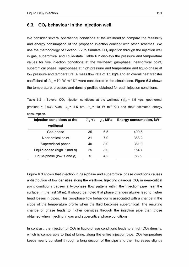
Liquid CO2 Injection 121
6.3. CO2 behaviour in the injection well
We consider several operational conditions at the wellhead to compare the feasibility
and energy consumption of the proposed injection concept with other schemes. We
use the methodology of Section 6.2 to simulate CO2 injection through the injection well
in gas, supercritical and liquid-state. Table 6.2 displays the pressure and temperature
values for five injection conditions at the wellhead: gas-phase, near-critical point,
supercritical phase, liquid-phase at high pressure and temperature and liquid-phase at
low pressure and temperature. A mass flow rate of 1.5 kg/s and an overall heat transfer
coefficient of 10=∞U W m-2 K-1 were considered in the simulations. Figure 6.3 shows
the temperature, pressure and density profiles obtained for each injection conditions.
Table 6.2 – Several CO2 injection conditions at the wellhead ( injQ = 1.5 kg/s, geothermal
gradient = 0.033 ºC/m, pR = 4.5 cm, ∞U = 10 W m-2 K-1) and their estimated energy
consumption.
Injection conditions at the wellhead
T , ºC p , MPa Energy consumption, kW
Gas-phase 35 6.5 409.6
Near-critical point 31 7.0 368.2
Supercritical phase 40 8.0 361.9
Liquid-phase (high T and p) 25 8.0 154.7
Liquid-phase (low T and p) 5 4.2 83.6
Figure 6.3 shows that injection in gas-phase and supercritical phase conditions causes
a distribution of low densities along the wellbore. Injecting gaseous CO2 in near-critical
point conditions causes a two-phase flow pattern within the injection pipe near the
surface (in the first 50 m). It should be noted that phase changes always lead to higher
head losses in pipes. This two-phase flow behaviour is associated with a change in the
slope of the temperature profile when the fluid becomes supercritical. The resulting
change of phase leads to higher densities through the injection pipe than those
obtained when injecting in gas and supercritical phase conditions.
In contrast, the injection of CO2 in liquid-phase conditions leads to a high CO2 density,
which is comparable to that of brine, along the entire injection pipe. CO2 temperature
keeps nearly constant through a long section of the pipe and then increases slightly
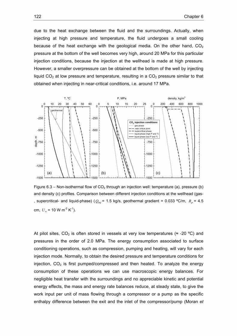
122 Chapter 6
due to the heat exchange between the fluid and the surroundings. Actually, when
injecting at high pressure and temperature, the fluid undergoes a small cooling
because of the heat exchange with the geological media. On the other hand, CO2
pressure at the bottom of the well becomes very high, around 20 MPa for this particular
injection conditions, because the injection at the wellhead is made at high pressure.
However, a smaller overpressure can be obtained at the bottom of the well by injecting
liquid CO2 at low pressure and temperature, resulting in a CO2 pressure similar to that
obtained when injecting in near-critical conditions, i.e. around 17 MPa.
P, MPa
0 5 10 15 20 25
-1500
-1250
-1000
-750
-500
-250
0
T, ºC
0 10 20 30 40 50 60
dept
h, m
-1500
-1250
-1000
-750
-500
-250
0
density, kg/m3
0 200 400 600 800 1000
-1500
-1250
-1000
-750
-500
-250
0geothermal
(a) (b) (c)
gas-phase
liquid-phase (high P and T)liquid-phase (low P and T)
CO2 injection conditions
supercritical phasenear critical point
Figure 6.3 – Non-isothermal flow of CO2 through an injection well: temperature (a), pressure (b)
and density (c) profiles. Comparison between different injection conditions at the wellhead (gas-
, supercritical- and liquid-phase) ( injQ = 1.5 kg/s, geothermal gradient = 0.033 ºC/m, pR = 4.5
cm, ∞U = 10 W m-2 K-1).
At pilot sites, CO2 is often stored in vessels at very low temperatures (≈ -20 ºC) and
pressures in the order of 2.0 MPa. The energy consumption associated to surface
conditioning operations, such as compression, pumping and heating, will vary for each
injection mode. Normally, to obtain the desired pressure and temperature conditions for
injection, CO2 is first pumped/compressed and then heated. To analyze the energy
consumption of these operations we can use macroscopic energy balances. For
negligible heat transfer with the surroundings and no appreciable kinetic and potential
energy effects, the mass and energy rate balances reduce, at steady state, to give the
work input per unit of mass flowing through a compressor or a pump as the specific
enthalpy difference between the exit and the inlet of the compressor/pump (Moran et
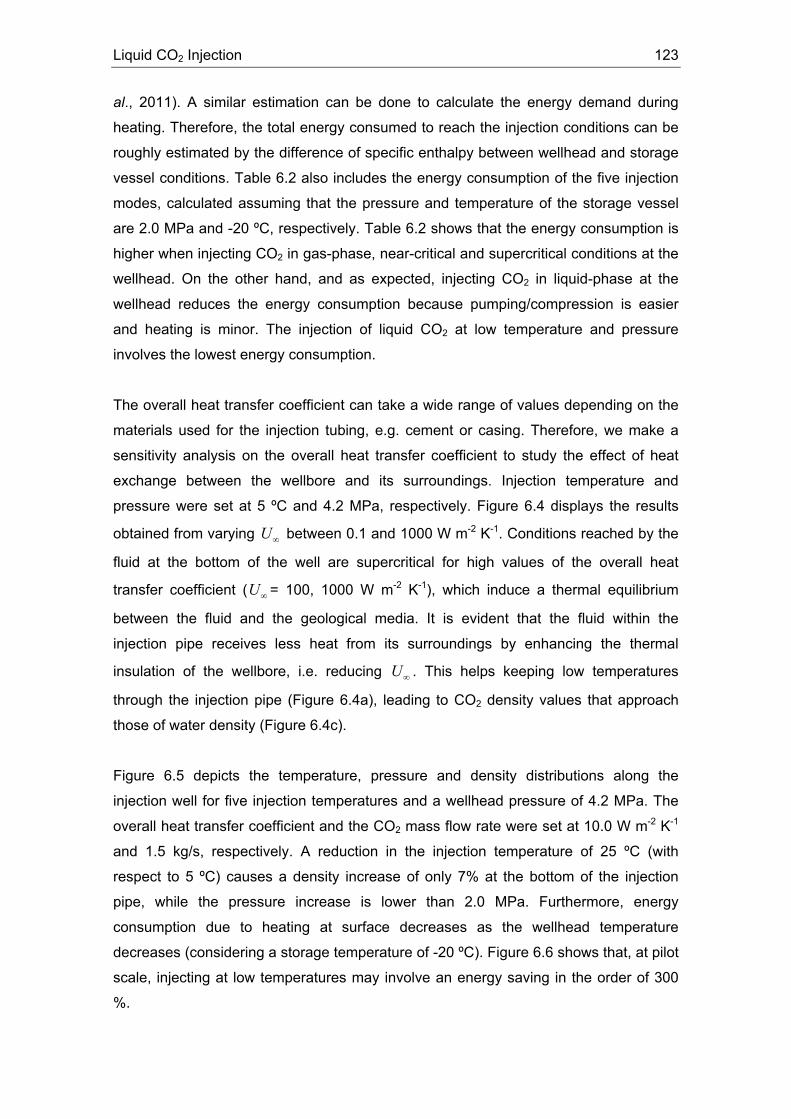
Liquid CO2 Injection 123
al., 2011). A similar estimation can be done to calculate the energy demand during
heating. Therefore, the total energy consumed to reach the injection conditions can be
roughly estimated by the difference of specific enthalpy between wellhead and storage
vessel conditions. Table 6.2 also includes the energy consumption of the five injection
modes, calculated assuming that the pressure and temperature of the storage vessel
are 2.0 MPa and -20 ºC, respectively. Table 6.2 shows that the energy consumption is
higher when injecting CO2 in gas-phase, near-critical and supercritical conditions at the
wellhead. On the other hand, and as expected, injecting CO2 in liquid-phase at the
wellhead reduces the energy consumption because pumping/compression is easier
and heating is minor. The injection of liquid CO2 at low temperature and pressure
involves the lowest energy consumption.
The overall heat transfer coefficient can take a wide range of values depending on the
materials used for the injection tubing, e.g. cement or casing. Therefore, we make a
sensitivity analysis on the overall heat transfer coefficient to study the effect of heat
exchange between the wellbore and its surroundings. Injection temperature and
pressure were set at 5 ºC and 4.2 MPa, respectively. Figure 6.4 displays the results
obtained from varying ∞U between 0.1 and 1000 W m-2 K-1. Conditions reached by the
fluid at the bottom of the well are supercritical for high values of the overall heat
transfer coefficient ( ∞U = 100, 1000 W m-2 K-1), which induce a thermal equilibrium
between the fluid and the geological media. It is evident that the fluid within the
injection pipe receives less heat from its surroundings by enhancing the thermal
insulation of the wellbore, i.e. reducing ∞U . This helps keeping low temperatures
through the injection pipe (Figure 6.4a), leading to CO2 density values that approach
those of water density (Figure 6.4c).
Figure 6.5 depicts the temperature, pressure and density distributions along the
injection well for five injection temperatures and a wellhead pressure of 4.2 MPa. The
overall heat transfer coefficient and the CO2 mass flow rate were set at 10.0 W m-2 K-1
and 1.5 kg/s, respectively. A reduction in the injection temperature of 25 ºC (with
respect to 5 ºC) causes a density increase of only 7% at the bottom of the injection
pipe, while the pressure increase is lower than 2.0 MPa. Furthermore, energy
consumption due to heating at surface decreases as the wellhead temperature
decreases (considering a storage temperature of -20 ºC). Figure 6.6 shows that, at pilot
scale, injecting at low temperatures may involve an energy saving in the order of 300
%.
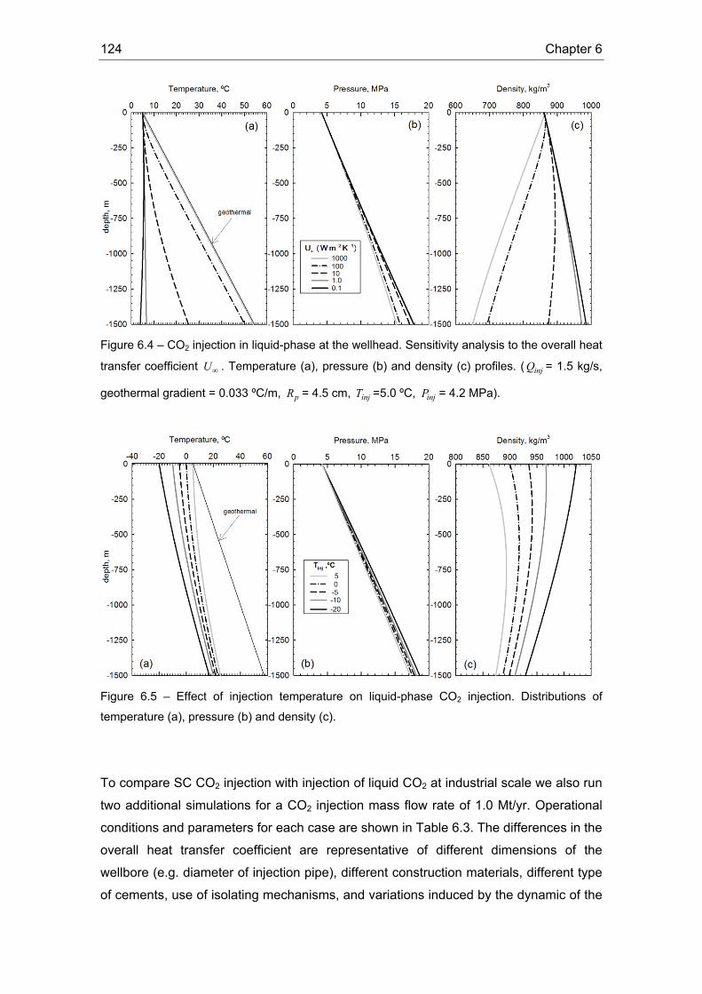
124 Chapter 6
Figure 6.4 – CO2 injection in liquid-phase at the wellhead. Sensitivity analysis to the overall heat
transfer coefficient ∞U . Temperature (a), pressure (b) and density (c) profiles. ( injQ = 1.5 kg/s,
geothermal gradient = 0.033 ºC/m, pR = 4.5 cm, injT =5.0 ºC, injP = 4.2 MPa).
Figure 6.5 – Effect of injection temperature on liquid-phase CO2 injection. Distributions of
temperature (a), pressure (b) and density (c).
To compare SC CO2 injection with injection of liquid CO2 at industrial scale we also run
two additional simulations for a CO2 injection mass flow rate of 1.0 Mt/yr. Operational
conditions and parameters for each case are shown in Table 6.3. The differences in the
overall heat transfer coefficient are representative of different dimensions of the
wellbore (e.g. diameter of injection pipe), different construction materials, different type
of cements, use of isolating mechanisms, and variations induced by the dynamic of the
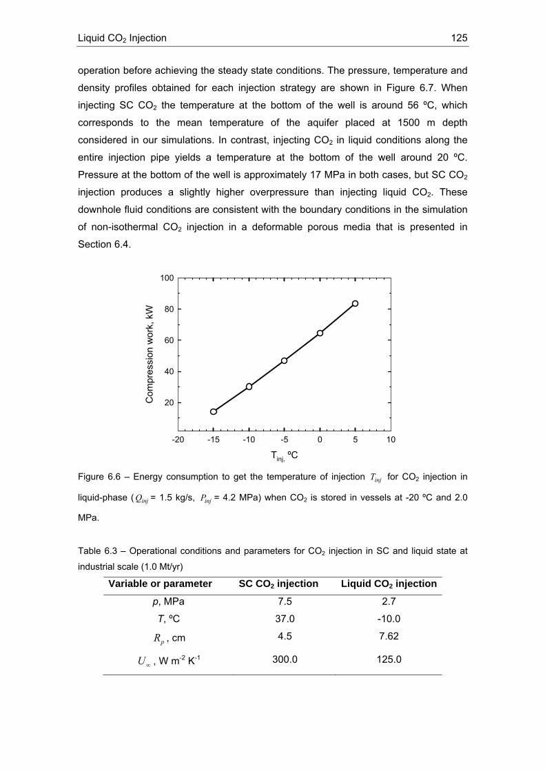
Liquid CO2 Injection 125
operation before achieving the steady state conditions. The pressure, temperature and
density profiles obtained for each injection strategy are shown in Figure 6.7. When
injecting SC CO2 the temperature at the bottom of the well is around 56 ºC, which
corresponds to the mean temperature of the aquifer placed at 1500 m depth
considered in our simulations. In contrast, injecting CO2 in liquid conditions along the
entire injection pipe yields a temperature at the bottom of the well around 20 ºC.
Pressure at the bottom of the well is approximately 17 MPa in both cases, but SC CO2
injection produces a slightly higher overpressure than injecting liquid CO2. These
downhole fluid conditions are consistent with the boundary conditions in the simulation
of non-isothermal CO2 injection in a deformable porous media that is presented in
Section 6.4.
Tinj, ºC-20 -15 -10 -5 0 5 10
Com
pres
sion
wor
k, k
W
20
40
60
80
100
Figure 6.6 – Energy consumption to get the temperature of injection injT for CO2 injection in
liquid-phase ( injQ = 1.5 kg/s, injP = 4.2 MPa) when CO2 is stored in vessels at -20 ºC and 2.0
MPa.
Table 6.3 – Operational conditions and parameters for CO2 injection in SC and liquid state at
industrial scale (1.0 Mt/yr)
Variable or parameter SC CO2 injection Liquid CO2 injection
p, MPa 7.5 2.7
T, ºC 37.0 -10.0
pR , cm 4.5 7.62
∞U , W m-2 K-1 300.0 125.0
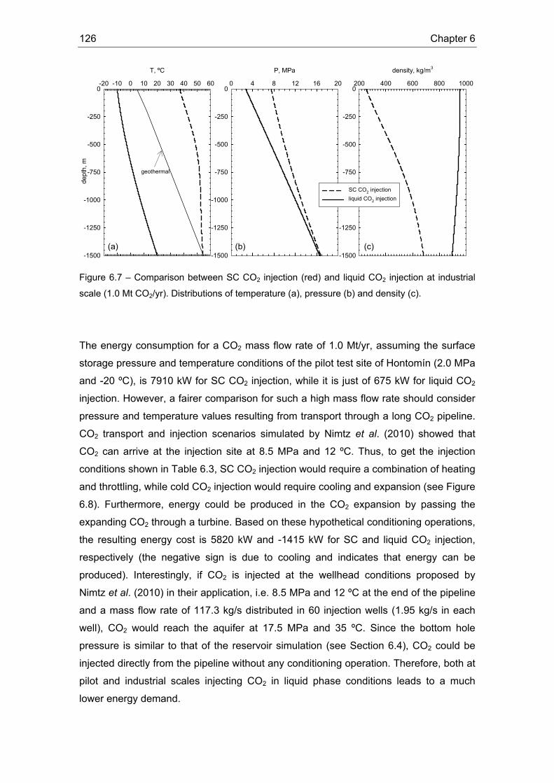
126 Chapter 6
T, ºC
-20 -10 0 10 20 30 40 50 60de
pth,
m
-1500
-1250
-1000
-750
-500
-250
0
density, kg/m3
200 400 600 800 1000
-1500
-1250
-1000
-750
-500
-250
0
geothermal
P, MPa
0 4 8 12 16 20
-1500
-1250
-1000
-750
-500
-250
0
SC CO2 injectionliquid CO2 injection
(a) (b) (c)
Figure 6.7 – Comparison between SC CO2 injection (red) and liquid CO2 injection at industrial
scale (1.0 Mt CO2/yr). Distributions of temperature (a), pressure (b) and density (c).
The energy consumption for a CO2 mass flow rate of 1.0 Mt/yr, assuming the surface
storage pressure and temperature conditions of the pilot test site of Hontomín (2.0 MPa
and -20 ºC), is 7910 kW for SC CO2 injection, while it is just of 675 kW for liquid CO2
injection. However, a fairer comparison for such a high mass flow rate should consider
pressure and temperature values resulting from transport through a long CO2 pipeline.
CO2 transport and injection scenarios simulated by Nimtz et al. (2010) showed that
CO2 can arrive at the injection site at 8.5 MPa and 12 ºC. Thus, to get the injection
conditions shown in Table 6.3, SC CO2 injection would require a combination of heating
and throttling, while cold CO2 injection would require cooling and expansion (see Figure
6.8). Furthermore, energy could be produced in the CO2 expansion by passing the
expanding CO2 through a turbine. Based on these hypothetical conditioning operations,
the resulting energy cost is 5820 kW and -1415 kW for SC and liquid CO2 injection,
respectively (the negative sign is due to cooling and indicates that energy can be
produced). Interestingly, if CO2 is injected at the wellhead conditions proposed by
Nimtz et al. (2010) in their application, i.e. 8.5 MPa and 12 ºC at the end of the pipeline
and a mass flow rate of 117.3 kg/s distributed in 60 injection wells (1.95 kg/s in each
well), CO2 would reach the aquifer at 17.5 MPa and 35 ºC. Since the bottom hole
pressure is similar to that of the reservoir simulation (see Section 6.4), CO2 could be
injected directly from the pipeline without any conditioning operation. Therefore, both at
pilot and industrial scales injecting CO2 in liquid phase conditions leads to a much
lower energy demand.

Liquid CO2 Injection 127
Figure 6.8 – CO2 diagram with the pressure-temperature trajectories of the surface operations,
in the injection well and inside the aquifer for the Hontomín surface storage conditions and for a
hypothetical CO2 transportation in a pipeline at industrial scale with an injection rate of 1 Mt/yr.
The results of the simulations presented in this section show that it is possible to inject
CO2 in dense liquid-phase by controlling the operational variables, which could lead to
a reduction of the reservoir overpressure and, theoretically, of the operational energetic
costs.
6.4. Thermo-hydro-mechanical effects of liquid CO2 injection
6.4.1. Thermal effects on CO2 plume evolution Liquid CO2 is denser and less viscous than SC CO2. This means that gravity forces
lose strength in front of viscous forces, which leads to a steeper CO2-brine interface
close to the injection well (Figure 6.9), where CO2 remains in liquid state (Figure
6.10a). Further away, where CO2 reaches SC conditions, the CO2 plume evolution is
characterized by gravity override (Nordbotten et al. 2005; Dentz and Tartakovsky,
2009a; Vilarrasa et al., 2010a) (Figure 6.9). The thermal transition is abrupt (Figure
6.10b). Once cold liquid CO2 enters in the aquifer, it heats up until thermal equilibrium
is reached, so that CO2 evolves to SC conditions as it flows away from the well.
Therefore, the liquid CO2 region is much smaller than the whole CO2 region. This leads
to a steep liquid CO2 front (where viscous forces dominate gravity forces) that

128 Chapter 6
advances behind the typical CO2 plume interface (where gravity forces dominate
viscous forces).
Figure 6.9 – CO2 plume after 1 year of injecting 1 Mt/yr of CO2 in (a) liquid and (b) supercritical
state.
Figure 6.10 – (a) CO2 density and (b) temperature after 8 months of liquid CO2 injection. CO2
remains in liquid state close to the injection well, leading to a steep front because viscous forces
dominate gravity forces. Once the CO2 thermally equilibrates with the medium (in a sharp front),
CO2 stays in SC state, leading to a CO2 plume interface dominated by gravity forces.

Liquid CO2 Injection 129
Apart from the cold CO2 injection, several processes affect the temperature distribution
of the CO2 plume. There is an interaction between: (1) the warmer CO2 placed at the
bottom of the aquifer flows upwards along the interface, (2) the colder brine placed at
the top of the aquifer flows downwards along the interface, (3) CO2 cools down as it
advances away from the injection well due to the Joule-Thomson effect and (4)
temperature increases due to the exothermal reaction of CO2 dissolution into the brine.
The net result of these processes is a slight temperature increase in the region of the
CO2 plume where CO2 stays in SC state (Figure 6.10b).
Figure 6.11a shows that injection pressure for liquid CO2 is slightly smaller than that of
SC CO2 because a higher CO2 density reduces the volumetric flow rate and therefore
the pressure buildup around the well. This is energetically advantageous, because a
smaller compression work has to be done to inject the same amount of CO2.
Furthermore, the overpressure in the whole aquifer becomes smaller (Figure 6.11b),
which improves the mechanical stability of the caprock.
1.0
1.2
1.4
1.6
0.0 0.2 0.4 0.6 0.8 1.0
Δp (M
Pa)
t (yr)
SC CO2 injection
Liquid CO2 injection
(a)
20
30
40
50
60
0.6
0.8
1.0
1.2
1.4
0.1 1 10 100 1000
Δp (M
Pa)
r (m)
SC CO2 injection
Liquid CO2 injection
Temperature(liquid CO2 injection)
(b)
Temperature
(ºC)
10‐1 100 101 102 103
Figure 6.11 – (a) Injection pressure evolution at the top of the aquifer for liquid and SC CO2
injection and (b) fluid pressure at the top of the aquifer as a function of radial distance from the
injection well after 1 yr of injection.
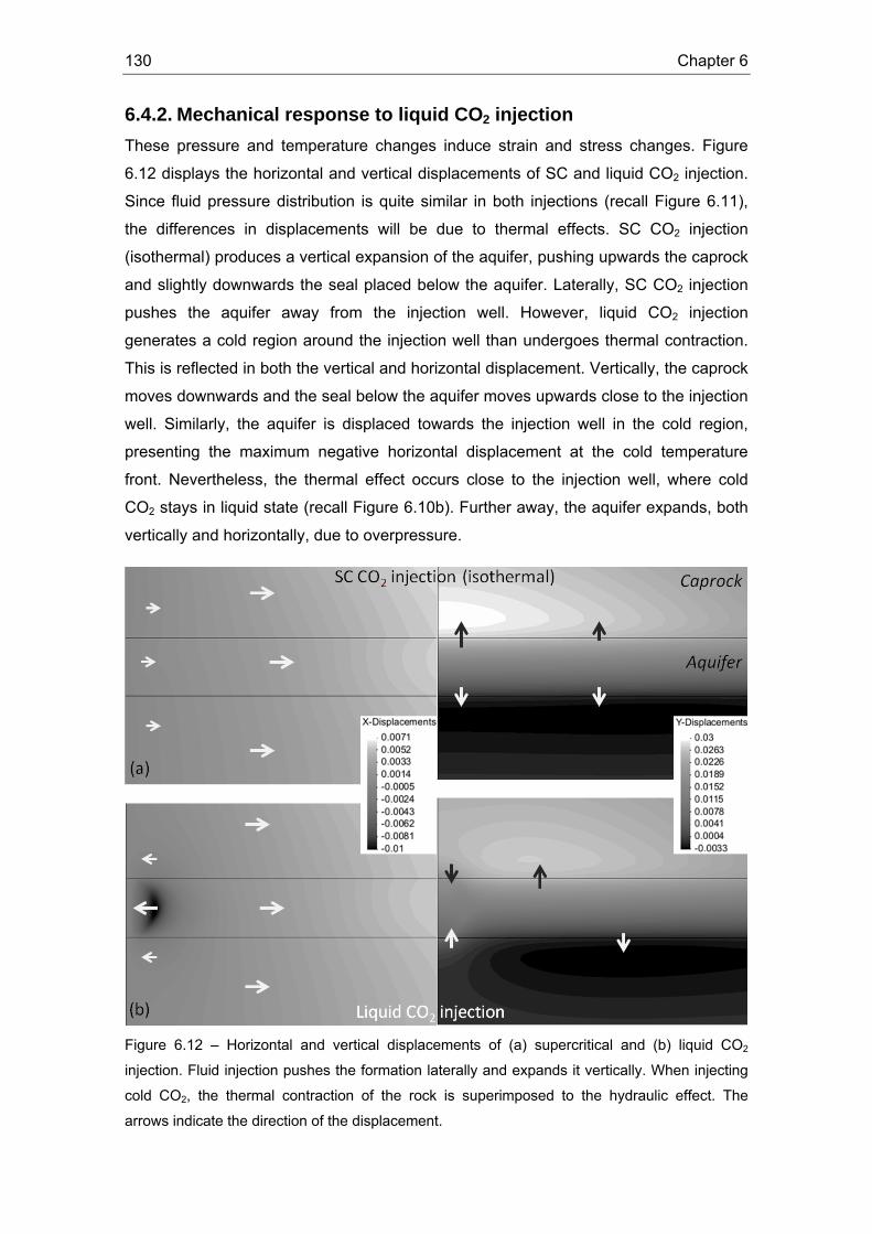
130 Chapter 6
6.4.2. Mechanical response to liquid CO2 injection These pressure and temperature changes induce strain and stress changes. Figure
6.12 displays the horizontal and vertical displacements of SC and liquid CO2 injection.
Since fluid pressure distribution is quite similar in both injections (recall Figure 6.11),
the differences in displacements will be due to thermal effects. SC CO2 injection
(isothermal) produces a vertical expansion of the aquifer, pushing upwards the caprock
and slightly downwards the seal placed below the aquifer. Laterally, SC CO2 injection
pushes the aquifer away from the injection well. However, liquid CO2 injection
generates a cold region around the injection well than undergoes thermal contraction.
This is reflected in both the vertical and horizontal displacement. Vertically, the caprock
moves downwards and the seal below the aquifer moves upwards close to the injection
well. Similarly, the aquifer is displaced towards the injection well in the cold region,
presenting the maximum negative horizontal displacement at the cold temperature
front. Nevertheless, the thermal effect occurs close to the injection well, where cold
CO2 stays in liquid state (recall Figure 6.10b). Further away, the aquifer expands, both
vertically and horizontally, due to overpressure.
Figure 6.12 – Horizontal and vertical displacements of (a) supercritical and (b) liquid CO2
injection. Fluid injection pushes the formation laterally and expands it vertically. When injecting
cold CO2, the thermal contraction of the rock is superimposed to the hydraulic effect. The
arrows indicate the direction of the displacement.
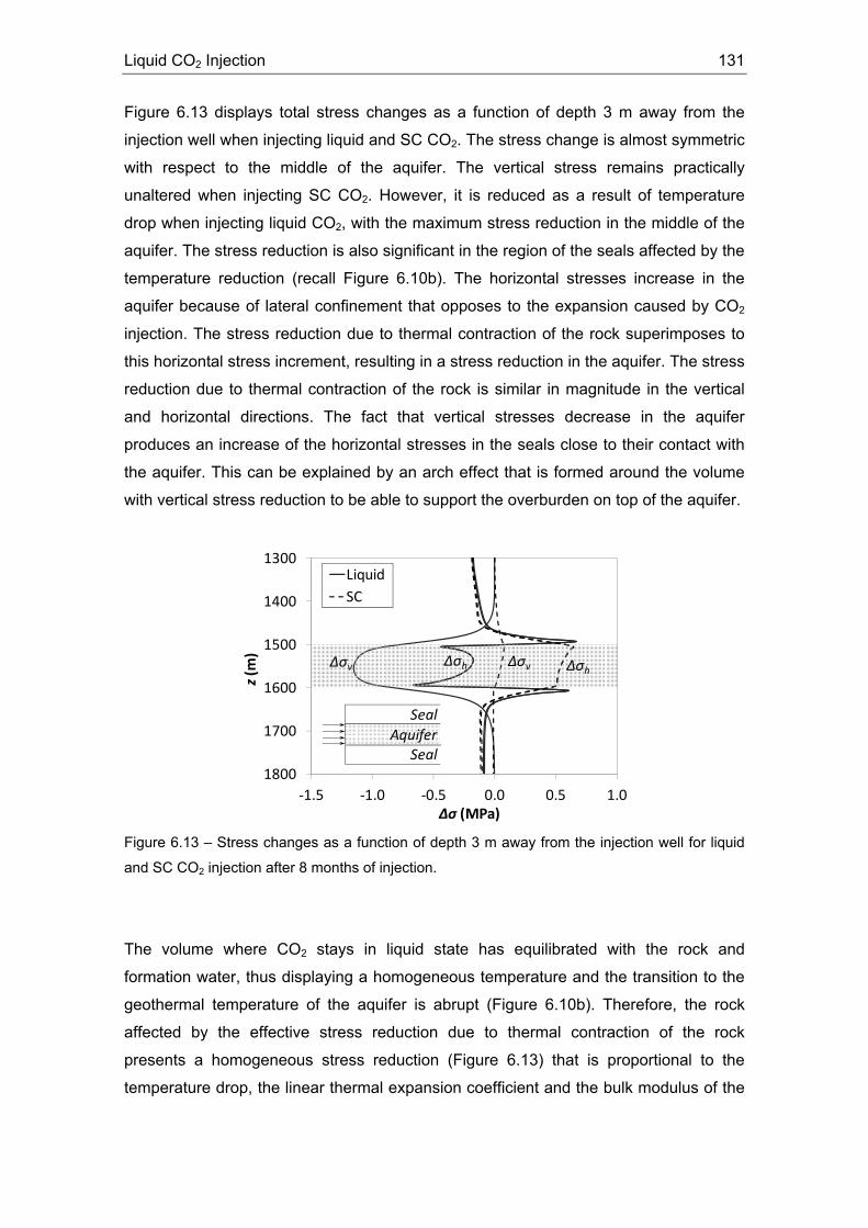
Liquid CO2 Injection 131
Figure 6.13 displays total stress changes as a function of depth 3 m away from the
injection well when injecting liquid and SC CO2. The stress change is almost symmetric
with respect to the middle of the aquifer. The vertical stress remains practically
unaltered when injecting SC CO2. However, it is reduced as a result of temperature
drop when injecting liquid CO2, with the maximum stress reduction in the middle of the
aquifer. The stress reduction is also significant in the region of the seals affected by the
temperature reduction (recall Figure 6.10b). The horizontal stresses increase in the
aquifer because of lateral confinement that opposes to the expansion caused by CO2
injection. The stress reduction due to thermal contraction of the rock superimposes to
this horizontal stress increment, resulting in a stress reduction in the aquifer. The stress
reduction due to thermal contraction of the rock is similar in magnitude in the vertical
and horizontal directions. The fact that vertical stresses decrease in the aquifer
produces an increase of the horizontal stresses in the seals close to their contact with
the aquifer. This can be explained by an arch effect that is formed around the volume
with vertical stress reduction to be able to support the overburden on top of the aquifer.
1300
1400
1500
1600
1700
1800‐1.5 ‐1.0 ‐0.5 0.0 0.5 1.0
z(m
)
Δσ (MPa)
LiquidSC
Δσv Δσh
Aquifer
Δσv Δσh
Seal
Seal
Figure 6.13 – Stress changes as a function of depth 3 m away from the injection well for liquid
and SC CO2 injection after 8 months of injection.
The volume where CO2 stays in liquid state has equilibrated with the rock and
formation water, thus displaying a homogeneous temperature and the transition to the
geothermal temperature of the aquifer is abrupt (Figure 6.10b). Therefore, the rock
affected by the effective stress reduction due to thermal contraction of the rock
presents a homogeneous stress reduction (Figure 6.13) that is proportional to the
temperature drop, the linear thermal expansion coefficient and the bulk modulus of the

132 Chapter 6
rock (Eq. (6.8)). Thus, the thermal effect will dominate for large temperature contrasts
and in stiff rocks.
6.4.3. Mechanical stability related to liquid CO2 injection Fluid injection induces an effective stress reduction that brings the stress state closer to
the failure envelope. Furthermore, if the fluid is colder than the formation, a thermal
contraction of the rock will occur, reducing even more the effective stresses. However,
liquid CO2 injection benefits from a lower overpressure for a given mass flow rate
(Figure 6.11). Therefore, coupled thermo-hydro-mechanical effects of liquid CO2
injection should be evaluated simultaneously to properly assess the mechanical
stability of the aquifer and the caprock.
Figure 6.14 compares the mobilized friction angle along the vertical at a radial distance
of 3 m away from the injection well when injecting liquid and SC CO2 for two values of
the lateral earth pressure coefficient. The mobilized friction angle in the aquifer is
higher for liquid CO2 injection than for SC CO2 injection. However, the opposite occurs
at the seals close to their contact with the aquifer when injecting liquid CO2 for a lateral
earth pressure coefficient of 0.5 (Figure 6.14a). This is because when the lateral earth
pressure coefficient is lower than 1.0, the maximum principal stress is the vertical.
Therefore, if the vertical stress is reduced and the horizontal stress increases (recall
Figure 6.13), the Mohr circle becomes smaller, leading to a more stable situation with a
smaller mobilized friction angle. The opposite occurs in the aquifer, where the vertical
and horizontal stresses are reduced and therefore the Mohr circle shifts to the left,
mobilizing higher friction angles. On the other hand, a lateral earth pressure coefficient
higher than 1.0 implies a vertical stress smaller than the horizontal stresses. In this
situation, a decrease in the vertical stress higher than in the horizontal stress makes
the Mohr circle bigger, mobilizing higher friction angles (Figure 6.14b). This trend is
only altered in the aquifer close to the contact with the seals, where the reduction in
horizontal stress is higher than in vertical stress, leading to a local minimum of the
mobilized friction angle in the aquifer.
If the mobilized friction angle becomes higher than the actual friction angle, shear slip
of critically oriented pre-existing fractures will occur, which would trigger microseismic
events. The effect of shear slip can be advantageous while it takes place within the
aquifer, because it can enhance permeability, especially in the direction perpendicular
to shear due to dilatancy (Yeo et al., 1998; Mallikamas and Rajaram, 2005; Vilarrasa et
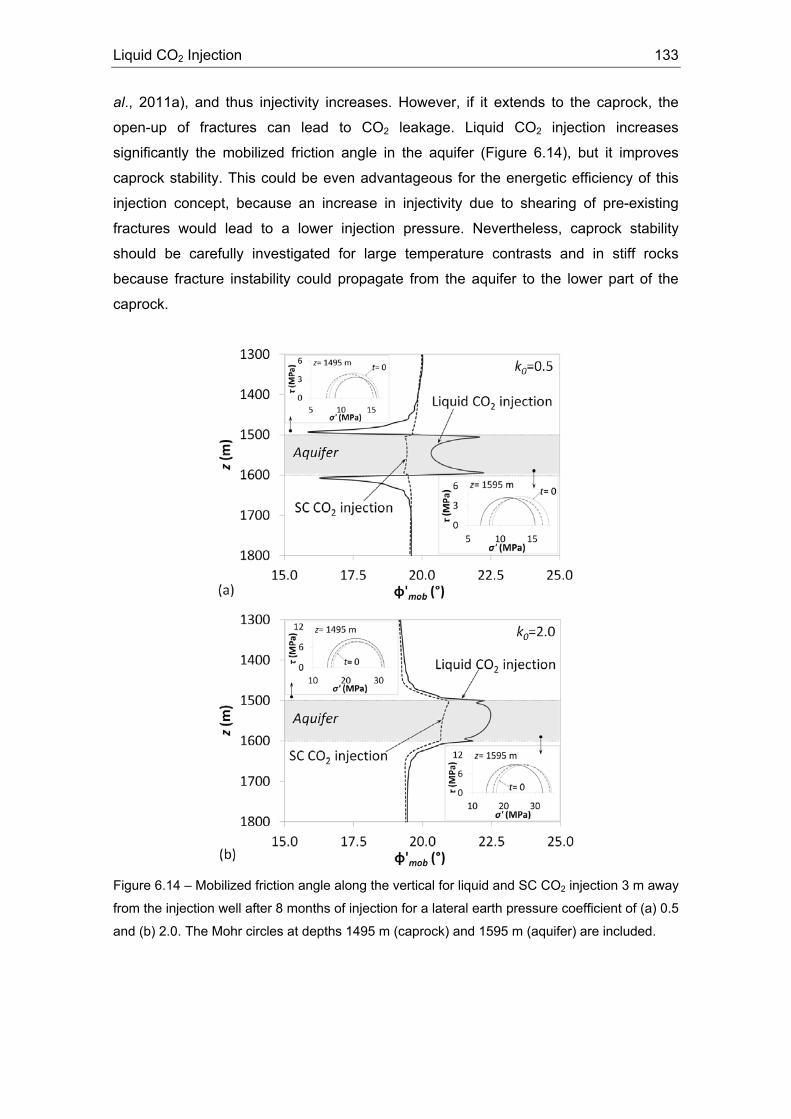
Liquid CO2 Injection 133
al., 2011a), and thus injectivity increases. However, if it extends to the caprock, the
open-up of fractures can lead to CO2 leakage. Liquid CO2 injection increases
significantly the mobilized friction angle in the aquifer (Figure 6.14), but it improves
caprock stability. This could be even advantageous for the energetic efficiency of this
injection concept, because an increase in injectivity due to shearing of pre-existing
fractures would lead to a lower injection pressure. Nevertheless, caprock stability
should be carefully investigated for large temperature contrasts and in stiff rocks
because fracture instability could propagate from the aquifer to the lower part of the
caprock.
Figure 6.14 – Mobilized friction angle along the vertical for liquid and SC CO2 injection 3 m away
from the injection well after 8 months of injection for a lateral earth pressure coefficient of (a) 0.5
and (b) 2.0. The Mohr circles at depths 1495 m (caprock) and 1595 m (aquifer) are included.
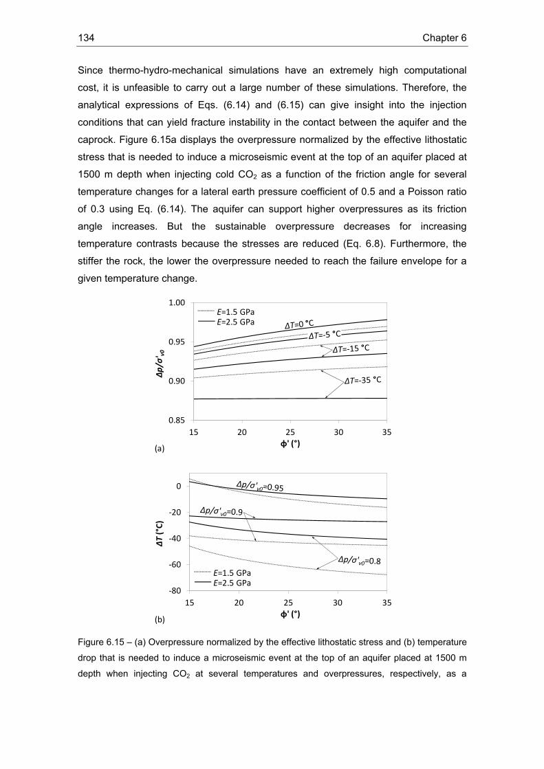
134 Chapter 6
Since thermo-hydro-mechanical simulations have an extremely high computational
cost, it is unfeasible to carry out a large number of these simulations. Therefore, the
analytical expressions of Eqs. (6.14) and (6.15) can give insight into the injection
conditions that can yield fracture instability in the contact between the aquifer and the
caprock. Figure 6.15a displays the overpressure normalized by the effective lithostatic
stress that is needed to induce a microseismic event at the top of an aquifer placed at
1500 m depth when injecting cold CO2 as a function of the friction angle for several
temperature changes for a lateral earth pressure coefficient of 0.5 and a Poisson ratio
of 0.3 using Eq. (6.14). The aquifer can support higher overpressures as its friction
angle increases. But the sustainable overpressure decreases for increasing
temperature contrasts because the stresses are reduced (Eq. 6.8). Furthermore, the
stiffer the rock, the lower the overpressure needed to reach the failure envelope for a
given temperature change.
0.85
0.90
0.95
1.00
15 20 25 30 35
Δp/σ' v0
φ' (°)
E=1.5 GPaE=2.5 GPa
(a)
‐80
‐60
‐40
‐20
0
15 20 25 30 35
ΔT (°C)
φ' (°)
E=1.5 GPaE=2.5 GPa
(b)
Figure 6.15 – (a) Overpressure normalized by the effective lithostatic stress and (b) temperature
drop that is needed to induce a microseismic event at the top of an aquifer placed at 1500 m
depth when injecting CO2 at several temperatures and overpressures, respectively, as a
Liquid CO2 Injection 135
function of the friction angle for a lateral earth pressure coefficient of 0.5 and a Poisson ratio of
0.3 given by Eq. (6.14) and (6.15) respectively.
Figure 6.15b displays the temperature change that is needed to induce a microseismic
event at the top of an aquifer placed at 1500 m depth when injecting cold CO2 as a
function of the friction angle for several overpressures for a lateral earth pressure
coefficient of 0.5 and a Poisson ratio of 0.3 using Eq. (6.15). The maximum acceptable
temperature change becomes higher for a given overpressure as the friction angle
increases. Furthermore, the stiffer the rock, the smaller the temperature change
required for inducing microseismicity for a given overpressure. Figure 6.15 can be used
as a reference to assess the feasibility of injecting liquid CO2 at a given site, once the
rigidity of the rock and the temperature change are known. Since there are 3D effects
that have not been considered in the analytical treatment of the problem, Figure 6.15
should be used only for guidance. However, its use is strongly recommended as a
preliminary analysis of the suitability of liquid CO2 injection at a given site because they
avoid performing coupled thermo-hydro-mechanical simulations, which imply a high
computational cost.
6.5. Conclusions
We propose to inject CO2 in liquid state. This is favourable for several reasons: (1) this
injection strategy is energetically advantageous, (2) no transformation operation or low
energy consumption conditioning operations are necessary, (3) a smaller compression
work is necessary because of the smaller compressibility of liquid CO2, (4) since liquid
CO2 is denser than SC CO2, liquid CO2 injection induces a lower overpressure because
a smaller amount of fluid is displaced and (5) the caprock mechanical stability is
improved.
Although relatively simple as a concept, the implementation of the operation may
require a thoroughly design of conditioning systems (e.g. throttling, heating or cooling)
to get the injection conditions. Nevertheless, the system is relatively easy to control
because direct control variables are the injection temperature and pressure.
Additionally, the system may be indirectly controlled by a suitable design of the
wellbore materials (e.g. cement, casing) to reduce the heat transfer between the pipe
and the surroundings, thus ensuring that the CO2 remains in liquid state along the
entire injection pipe. Since, in general, the temperature at which CO2 will reach the
136 Chapter 6
aquifer will be different than that of the aquifer, non-isothermal simulations should be
performed to reproduce realistic injection conditions.
As for the mechanical stability of the rocks, the thermal effect is more pronounced for
large temperature contrasts and in stiff rocks. Thermal contraction mobilizes higher
friction angles in the aquifer, which could lead to shear slip of pre-existing fractures.
The effect of shear slip can be advantageous while it takes place within the aquifer,
because it enhances permeability and thus CO2 injectivity. Interestingly, the mobilized
friction angle in the seals is not increased when injecting liquid CO2 and it is even
reduced in stress regimes where the maximum principal stress is the vertical.
137
7. Conclusions
This Thesis deals with several coupled effects related to CO2 sequestration, including
two-phase flow, hydromechanical coupling and thermo-hydro-mechanical coupling. The
main conclusions drawn from this Thesis are summarized below.
Analytical solutions are useful because they provide a quick solution and help identify
relevant parameters pertaining to a particular problem. However, current analytical
solutions for the geometry of a CO2 plume make several oversimplifying assumptions
that we attempt to relax. These include the incompressibility of CO2 and the uniform
injection of CO2 along the entire thickness of the aquifer. We have relaxed the former
assumption by introducing an iterative method that corrects the initial estimate of CO2
density and viscosity and hence ends up using more realistic values. We have found
that the error associated with neglecting compressibility increases dramatically when
gravity forces dominate, which is likely to occur at late times of injection. Comparison
with numerical simulations suggests that the previously published solution of
Nordbotten et al. (2005) gives good predictions for the CO2 plume position when
viscous forces dominate, while the solution of Dentz and Tartakovsky (2009a) provides
better estimates when gravity forces dominate. Additionally, we have developed a
semianalytical solution that takes into account both CO2 compressibility and buoyancy
effects within the injection well. Therefore, CO2 is not necessarily injected along the
entire thickness of the aquifer. The CO2 plume geometry and fluid overpressure
obtained from the semianalytical solution are in good agreement with high resolution
numerical solutions. However, the computational cost and time to complete the
calculations is minimal compared to these numerical solutions.
Fluid overpressure induces deformations of the aquifer and the caprock. When
injecting a constant CO2 mass flow rate in a vertical well, fluid pressure builds up
sharply at the beginning of injection both because the viscosity of the displaced brine is
high and because the permeability to brine is reduced due to desaturation. However,
once CO2 fills the pores in the vicinity of the injection well and a capillary fringe is fully
developed, the pressure within the CO2 plume slowly decreases both because the flux

138 Chapter 7
across the fringe is reduced (it is inversely proportional to the radius of the capillary
fringe) and because the viscosity of CO2 is much lower than that of the brine. As a
result, mechanical stability tends to improve. However, in the presence of a low-
permeability boundary, brine pressure rises once the radius of influence reaches the
outer boundary, which causes the CO2 pressure to rise and could compromise the
mechanical integrity of the caprock in the long-term. A conclusion from this analysis is
that the risk of damage to the caprock is reduced if the injection rate is progressively
increased at the beginning of injection.
The mechanical response of the aquifer and caprock to the fluid pressure perturbations
depends on their mechanical properties, i.e. the Young’s modulus and the Poisson
ratio. These parameters are usually measured at the laboratory. However, values
measured at the laboratory scale may not be representative of effective values at the
field scale. Thus, we propose a hydromechanical characterization test to determine the
aquifer and caprock hydromechanical properties at the field scale. This test permits
also the determination of the maximum sustainable injection pressure, defined as the
pressure that causes the onset of microseismicity in the caprock. We obtain curves for
overpressure and vertical displacement as a function of the volumetric strain term
obtained from a dimensional analysis of the hydromechanical equations. These curves
show the hydromechanical behaviour of the aquifer-caprock system when injecting a
fluid, but more importantly, they can also be used for parameter estimation from field
measurements. Overall, this test will help assess the suitability of specific CO2 storage
sites and will allow practitioners to obtain representative effective values of
hydromechanical parameters at the field scale.
We also propose a new injection strategy that is energetically advantageous and that
improves the caprock mechanical stability in some situations, which consists of
injecting CO2 in liquid state. Liquid (cold) CO2 is denser than supercritical CO2.
Therefore, the pressure required at the wellhead for a given CO2 pressure at the
aquifer is much lower for liquid than for gas or supercritical injection. Actually, the
overpressure required at the aquifer is also smaller because a smaller fluid volume is
displaced. Furthermore, since CO2 is transported through pipelines in liquid state, CO2
could be injected directly as it arrives to the wellhead or after conditioning operations of
low energy cost. Thus, this injection strategy is energetically efficient. Apart from this,
the injected liquid CO2 will cool the reservoir around the injection well, inducing a stress
reduction due to thermal contraction of the rock. The thermal effect becomes greater
for larger temperature contrasts and for stiffer rocks. The thermal contraction of the

Conclusions 139
rock mobilizes higher friction angles, which could lead to shear slip of pre-existing
fractures. Shear slip enhances fracture permeability, which is advantageous for CO2
injection while it occurs within the aquifer. This is likely to occur when injecting liquid
CO2, because, interestingly, the mobilized friction angle in the caprock is not increased
and is even reduced in stress regimes where the maximum principal stress is the
vertical.


141
Appendices


143
I. Mean CO2 density
Here, the mean CO2 density defined in Eq. (2.16) is calculated using the linear
approximation of CO2 density with respect to pressure presented in Eq. (2.20) for both
approaches, i.e. Nordbotten et al. (2005) and Dentz and Tartakovsky (2009a).
With the Nordbotten et al. (2005) approach, the mean CO2 density is calculated by
introducing (2.11) and (2.17) into (2.16), which leads to
⎪⎭
⎪⎬⎫
⎪⎩
⎪⎨⎧
⎥⎥⎦
⎤
⎢⎢⎣
⎡
⎥⎥⎦
⎤
⎢⎢⎣
⎡⎟⎟⎠
⎞⎜⎜⎝
⎛−−⎟⎟
⎠
⎞⎜⎜⎝
⎛+⎟⎟
⎠
⎞⎜⎜⎝
⎛++=
w
cbb
ww
bbcN
rrRrr
kQgdrrrrd
V μμ
πμρβρρπϕρ
211
631ln
21
2422 2
00
020100 .
(I.1)
Similarly, introducing (2.13) and (2.18) into (2.16), and integrating, yields the
expression for the mean CO2 density for the Dentz and Tartakovsky (2009a) approach,
⎭⎬⎫
⎟⎟⎠
⎞⎜⎜⎝
⎛−−
⎥⎥⎦
⎤
⎢⎢⎣
⎡⎟⎟⎠
⎞⎜⎜⎝
⎛⎟⎟⎠
⎞⎜⎜⎝
⎛ ++⎟⎟
⎠
⎞⎜⎜⎝
⎛++
⎪⎩
⎪⎨⎧
⎥⎦
⎤⎢⎣
⎡−⎟⎟
⎠
⎞⎜⎜⎝
⎛=
wb
cwwcw
b
cw
bww
cwcw
b
cwcDT
kdQdrgdr
rR
kdQgddr
V
μπ
βργ
βρργ
μμμπ
ργβρργγ
πϕρ
242exp
4
2ln
22412exp2
01
2
12
2
010
2
(I.2)


145
II. Implementation of CO2 properties
in CODE_BRIGHT
CODE_BRIGHT has been extended to simulate non-isothermal CO2 injection. To do
so, the Redlich and Kwong (1949) equation of state with the parameters proposed for
CO2 by Spycher et al. (2003) has been implemented. This equation of state is a cubic
equation of the molar volume
0223 =⎟⎟⎠
⎞⎜⎜⎝
⎛−⎟⎟
⎠
⎞⎜⎜⎝
⎛+−−⎟⎟
⎠
⎞⎜⎜⎝
⎛−
TpabVb
Tpa
pRTbV
pRTV
cccc
, (II.1)
where V is molar volume, R is the gas constant, T is temperature, cp is CO2
pressure and a and b represent measures of intermolecular attraction and repulsion,
respectively. Note that if ba = = 0, the ideal gas law is recovered.
Spycher et al. (2003) assumed that
Taaa 10 += , (II.2)
and adjust 0a , 1a and b to experimental TVpc −− data. For pure CO2 these
constants are 20.56
0 /molKmPa 54.7 ⋅⋅=a , (II.3a)
20.5631 /molK/mPa 1013.4 ⋅⋅−= −a , (II.3b)
mol/m 1078.2 35−⋅=b . (II.3c)
Given a CO2 pressure cp and a temperature T , the cubic equation Eq. (II.1) can be
solved directly for V by following a method like the one proposed by Nickalls (1993).
Once the molar volume V is known, CO2 density, cρ , is calculated as
VMCO
c2=ρ , (II.4)
where 2COM = 0.044 kg/mol is the CO2 molecular weight. Figure II.1 shows CO2
density calculated according to this equation of state for several temperatures (sub and
supercritical) and up to 40 MPa.
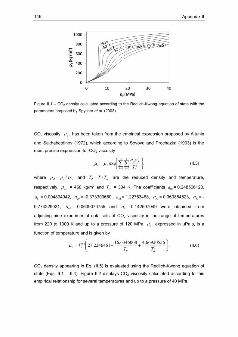
146 Appendix II
0
200
400
600
800
1000
0 10 20 30 40
ρ c(kg/m
3 )
pc (MPa)
Figure II.1 – CO2 density calculated according to the Redlich-Kwong equation of state with the
parameters proposed by Spycher et al. (2003).
CO2 viscosity, cμ , has been taken from the empirical expression proposed by Altunin
and Sakhabetdinov (1972), which according to Sovova and Prochazka (1993) is the
most precise expression for CO2 viscosity
⎟⎟⎠
⎞⎜⎜⎝
⎛= ∑∑
= =
4
1
1
00 exp
i jjR
iRij
c Ta ρ
μμ , (II.5)
where crcR ρρρ /= and crR TTT /= are the reduced density and temperature,
respectively, crρ = 468 kg/m3 and crT = 304 K. The coefficients 10a = 0.248566120,
11a = 0.004894942, 20a = -0.373300660, 21a = 1.22753488, 30a = 0.363854523, 31a = -
0.774229021, 40a = -0.0639070755 and 41a = 0.142507049 were obtained from
adjusting nine experimental data sets of CO2 viscosity in the range of temperatures
from 220 to 1300 K and up to a pressure of 120 MPa. 0μ , expressed in μPa·s, is a
function of temperature and is given by
⎟⎟⎠
⎞⎜⎜⎝
⎛+−= 2
5.00
66920556.46346068.162246461.27RR
R TTTμ . (II.6)
CO2 density appearing in Eq. (II.5) is evaluated using the Redlich-Kwong equation of
state (Eqs. II.1 – II.4). Figure II.2 displays CO2 viscosity calculated according to this
empirical relationship for several temperatures and up to a pressure of 40 MPa.

Implementation in CODE_BRIGHT 147
0.E+00
3.E‐05
6.E‐05
9.E‐05
1.E‐04
0 10 20 30 40
μ c(Pa∙s)
pc (MPa)
0.0
3.0∙10‐5
6.0∙10‐5
9.0∙10‐5
1.2∙10‐5
Figure II.2 – CO2 viscosity calculated according to the empirical expression proposed by Altunin
and Sakhabetdinov (1972).
Additionally, water density increment due to CO2 dissolution has been implemented
following the methodology proposed by Garcia (2003). Water density, wρ , is
proportional to the dissolved CO2 and a coefficient δ that accounts for the fact that the
dissolved CO2 occupies a certain volume
( )( )( )clwwwww Tpp δωαβρρ ++−= 1exp 00 , (II.7)
where 0wρ is a reference water density corresponding to the reference water pressure
0wp , β is water compressibility, wp is water pressure, wα is water volumetric thermal
expansion coefficient, clω is the CO2 mass fraction in liquid and δ is
( )( )2
00 exp1CO
wwww MV
Tpp φαβρδ +−−= , (II.8)
where φV is the apparent molar volume of dissolved CO2. φV , expressed in m3/mol, is a
function of temperature (in ºC) and is equal to
( ) 637242 1010044.51074.810585.951.37 −−−− ⋅−⋅+⋅−= TTTVφ . (II.9)
The specific enthalpy of CO2, ch , can be evaluated integrating the fundamental
thermodynamic relationship
cp
pc dpTVTVdTcdh
⎥⎥⎦
⎤
⎢⎢⎣
⎡⎟⎠⎞
⎜⎝⎛∂∂
−+= , (II.10)

148 Appendix II
where pc is the specific heat capacity at constant pressure, and the molar volume of
CO2, V , can be calculated using the Redlich-Kwong equation of state of Eqs. (II.1) to
(II.4). At constant temperature, Eq. (II.10) reduces to
cp
c dpTVTVdh
⎥⎥⎦
⎤
⎢⎢⎣
⎡⎟⎠⎞
⎜⎝⎛∂∂
−= . (II.11)
Integrating Eq. (II.11) between a reference pressure, e.g. atmospheric pressure, and a
CO2 pressure cp yields
( ) ( ) ∫⎥⎥⎦
⎤
⎢⎢⎣
⎡⎟⎠⎞
⎜⎝⎛∂∂
−=− ∗ cp
cp
ccc dpTVTVThTph
0, , (II.12a)
or
( ) ( ) ( ) ∫∞∗
⎥⎦
⎤⎢⎣
⎡−⎟
⎠⎞
⎜⎝⎛∂∂
+−=−V
cV
cccc dVp
TpTZRTThTph 1, , (II.12b)
where ∗ch is the enthalpy of an ideal gas at atmospheric pressure, which only depends
on temperature and Z is the compressibility factor. Adopting the Redlich-Kwong
equation of state with the parameters proposed by Spycher et al. (2003), Eq. (II.12)
becomes
( ) ( ) 21
0* 1ln5.1,, COcccc M
Vb
bTTaaRTVpTphTph ⎟⎟
⎠
⎞⎜⎜⎝
⎛⎟⎠⎞
⎜⎝⎛ +
−−−=− , (II.13)
where temperature expressed in K, molar volume in m3/mol and gas pressure in Pa
gives enthalpy in J/kg. Figure II.3 shows the CO2 enthalpy calculated from Eq. (II.13)
for several temperatures up to a CO2 pressure of 40 MPa.
Once the CO2 enthalpy is determined through Eq. (II.13), the CO2 specific heat
capacity can be calculated from its definition
p
cp T
hc ⎟⎠⎞
⎜⎝⎛∂∂
= . (II.14)
Applying Eq. (II.14) with the expression of the enthalpy given by Eq. (II.13) yields
( )( ) 2
13
0* 5.11ln75.0,
COcp MTV
VbVTTaa
Vb
TbaR
TVp
TTphc ⎟⎟
⎠
⎞⎜⎜⎝
⎛∂∂
+−
+⎟⎠⎞
⎜⎝⎛ ++−
∂∂
+∂
∂= , (II.15)
where
( )( ) ( )cc pbTaRTbVRTpV
TTaabTTaaRbVRVTV
22
31
31
2
/23/5.0/5.0
+−++−−−−+
=∂∂ , (II.16)

Implementation in CODE_BRIGHT 149
where temperature expressed in K, molar volume in m3/mol and gas pressure in Pa
gives the specific heat capacity in J/kg/K. Figure II.4 displays the CO2 specific heat
capacity calculated from Eq. (II.15) and (II.16).
‐3.0E+05
‐2.0E+05
‐1.0E+05
0.0E+00
1.0E+05
0 10 20 30 40
h c(J/kg)
pc (MPa)
‐3.0∙105
‐2.0∙105
‐1.0∙105
0.0
1.0∙105
Figure II.3 – CO2 enthalpy calculated from the Redlich-Kwong equation of state with the
parameters proposed by Spycher et al. (2003).
1.E+02
1.E+03
1.E+04
1.E+05
0 10 20 30 40
c p(J/kg/K)
pc (MPa)
300 K
290 K
310 K
320 K
330 K
340 K350 K
360 K
102
103
104
105
Figure II.4 – Specific heat capacity calculated from the Redlich-Kwong equation of state with the
parameters proposed by Spycher et al. (2003).
We also account for the enthalpy of dissolved CO2. According to Han et al. (2010), the
enthalpy of dissolved CO2, expressed in J/kg, is a function of temperature (in K),
( )2
3
2
64 1010475.7102634.656.106CO
cl MTTTh ⎟⎟
⎠
⎞⎜⎜⎝
⎛ ⋅+
⋅−= . (II.16)

150 Appendix II
McPherson et al. (2008) compared the Redlich-Kwong equation of state with that of
Span and Wagner (Span and Wagner, 1996). They show that the thermodynamic
properties given by Span and Wagner (1996) are almost identical to the International
Union of Pure and Applied Chemistry (IUPAC) (Angus et al., 1976) data sets over the
Tpc − range of CO2 sequestration interest. However, the algorithm given by Span and
Wagner (1996) for evaluating CO2 properties has a very high computational cost, being
around 100 times slower than that of the Redlich-Kwong equation of state (McPherson
et al., 2008). Additionally, the Redlich-Kwong equation of state is more flexible and
gives acceptable agreement with experimental data (McPherson et al., 2008).
Therefore, we chose to use the Redlich-Kwong equation of state.
151
III. Potential calculation
Here we develop the mathematical formulation of the problem for the case in which
CO2 density varies linearly with pressure (Eq. (3.24)), and CO2 viscosity and brine
properties are constant.
First, we integrate Eq. (3.4) for the CO2 phase, which yields
( )⎟⎟⎠
⎞⎜⎜⎝
⎛−++−= 0
00 1ln1 PPg
zzh cc ρβ
β. (III.1)
The inverse of Eq. (III.1) gives the CO2 pressure as a function of the head as
( )( )( )1000 −=− −− zzhg
ccePP β
βρ
. (III.2)
Integrating Eq. (3.12) and using Eq. (III.2) gives the following expression for the CO2
potential
( )( )12220 0 −=Φ −− chgzzg
cc eek ββ
βμρπ
. (III.3)
Since the exponent chgβ2 is small, ( )12 −chge β can be approximated as chgβ2 .
Therefore, the CO2 potential can be expressed as
( )0220 2 zzg
cc
c ehgk −−≈Φ β
μρπ , (III.4)
where the potential is composed of a part corresponding to a constant CO2 density
( 0ρ ) multiplied by a correction due to CO2 compressibility (the exponential in the right-
hand side of Eq. (III.4)). Combining Eq. (III.1) and (III.3) and operating, yields an
expression of CO2 pressure as a function of the potential
( )
βρ
βρ
βπμ β 02
2
20
00 −+Φ=− −− zzg
cc
c ek
PP . (III.5)
Note that the head (Eq. (III.1)) at the interface can be expressed as a function of the
CO2 density as
152 Appendix III
( )⎟⎟⎠
⎞⎜⎜⎝
⎛+−=⎟⎟
⎠
⎞⎜⎜⎝
⎛ −++−=
00
0
000 ln1ln1
ρρ
βρβρ
βcici
ci gzzPP
gzzh , (III.6)
where the subscript i indicates interface. Combining Eq. (III.3) with Eq. (III.6) yields the
following expression for the CO2 potential at the interface
( )⎟⎟⎠
⎞⎜⎜⎝
⎛−=Φ −− 02
20
220 zzgci
ci ek β
ρρ
βμρπ
. (III.7)
In the brine phase, integration of Eq. (3.4) yields
gPPzzh
w
ww ρ
00
−+−= , (III.8)
which is the expression of the head for an incompressible fluid. Integrating Eq. (3.12)
gives the potential in the brine phase as
ww
ww hgk
μρπ
2
2=Φ . (III.9)
Combining Eq. (III.8) with (III.9), gives the following expression for the brine pressure
( ) gzzk
PP www
ww ρ
ρπμ
00 2−−Φ=− . (III.10)
Note that the brine pressure varies with the logarithm of the distance to the injection
well (see the form of the potential in Eq. (3.16a)).

153
IV. CO2 plume thickness calculation
A system of two equations with two unknowns has to be solved in step 4 of the time
stepping algorithm of Chapter 3 when a mass flow rate is prescribed at the injection
well. The unknowns are the head at the well and the thickness of the CO2 plume at the
well. The two equations are Eq. (3.23) and (3.8) accounting for the capillary entry
pressure in (3.6).
Combining Eq. (3.23) with Eqs. (3.18), (III.3) and (III.7), after some algebra, gives the
following expression for the head at the well as a function of the increment of the CO2
plume thickness
4
3212
AAAzAQ
e fhg c−+Δ−
=β , (IV.1)
where
mc Qk
Q 20ρπβμ
= , (IV.2a)
( )tSr
kA rwifcc
Δ−
=12
20
1
ϕπρρπβμ
, (IV.2b)
( ) j
m
j pj
jci zrr
A Δ=∑=1
20
2,
2 lnρρ
, (IV.2c)
( )( ) j
n
j pj
jjjczc zrrrrJ
kA Δ= ∑
=
++
1
11,20
3 lnln
ρπβμ
, (IV.2d)
( )
( ) j
m
j pj
zzg
zrr
eAj
Δ=∑=
−−
1
2
4 ln
0β
. (IV.2e)
Next, combining Eq. (3.6) with Eqs. (III.3), (III.5) and assuming hydrostatic conditions at
the well give the second equation of the system of equations
fwhg zgpe c Δ+= βρρβ
0
, (IV.3)
where
( )( ) 110
++= − ccfw PzPpρβ
, (IV.4)
154 Appendix IV
where ( )1−fw zP is the brine pressure evaluated at the depth reached by the CO2 plume
in the previous time step. The combination of Eq. (IV.1) and (IV.3) gives the following
quadratic equation
02 =+Δ+Δ CzBz ff , (IV.5)
where ( )
4
1222
2200
02AA
ge
gpB
w
zzg
w
f
βρρ
βρρ β −−
+= , (IV.6a)
( )⎟⎟⎠
⎞⎜⎜⎝
⎛ −+−= −− 02
4
322222
20 zzg
w
feA
AAQpg
C β
βρρ
. (IV.6b)
Once Eq. (IV.5) is solved and the increment of the CO2 plume thickness at the well in a
given time step is known, the head at the well can be calculated from Eq. (IV.1) as
( ) ⎟⎟⎠
⎞⎜⎜⎝
⎛ −+Δ−=
4
321exp2
1A
AAzAQg
rh fpc β
. (IV.7)
155
V. Mean CO2 density at a layer
The mean CO2 density in a given layer has to be calculated in order to apply Eq. (3.23).
Assuming that CO2 density varies linearly with pressure (Eq. (3.24)), and using Eq.
(III.5), (3.16c) and (III.7), after some algebra, the following expression for the CO2
density is obtained
rr
Jk
jc
ccic ln2
πβμρρ += . (V.1)
The mean CO2 density in a layer is obtained from dividing the CO2 mass in a given
layer by the volume that it occupies
( ) zrSrV
j
j
j
p
z
z
r
rcrw dd121
1
∫ ∫−
−= ρϕπρ . (V.2)
Introducing Eq. (V.1) in Eq. (V.2) and integrating yields
( )
( ) ⎥⎥⎦
⎤
⎢⎢⎣
⎡⎟⎟⎠
⎞⎜⎜⎝
⎛⎟⎟⎠
⎞⎜⎜⎝
⎛−⎟⎟
⎠
⎞⎜⎜⎝
⎛⎟⎟⎠
⎞⎜⎜⎝
⎛+−
−
=⎥⎥⎦
⎤
⎢⎢⎣
⎡⎟⎟⎠
⎞⎜⎜⎝
⎛−−−
−=
cpcicij
cppcijpj
r
r
ba
pj
berf
berf
bbr
rrrr
rbab
erfebrbarrr
j
p
ρρρπρρ
πρ
222exp22
1
ln222
1ln1
2222
22
/2222
, (V.3)
where
jcc
ci rJk
a ln2
πβμρ += , (V.4a)
cc Jk
bπβμ
= . (V.4b)

157
VI. Coupled HM formulation for CO2
flow
The balance equations required for the solution of the problems studied in Chapter 4
are presented in this appendix. Olivella et al. (1994) have presented the governing
equations for non-isothermal multiphase flow of water and gas through porous
deformable media. A detailed derivation is given there, and only a description of the
modified formulation for gas (CO2) flow is presented in this appendix.
The mass balance of solid present in the medium is written as
( )( ) ( ) 01 =⋅∇+− sstjφρ
∂∂
, (VI.1)
where sρ is the density of solid and sj is the flux of solid. From this equation, an
expression for porosity variation can be obtained if the flux of solid is written as the
velocity of the solid multiplied by the volumetric fraction occupied by the solid phase
and its density, i.e. td/d)1( ss uj ϕρ −= ,
( ) ( )tDt
DDtD ss
s
s
dd11 u⋅∇−+
−= ϕρ
ρϕϕ
. (VI.2)
The material derivative with respect to the solid is defined as
( ) ( ) ( )•∇⋅+∂•∂
=•
ttDtDs
ddu
. (VI.3)
Equation (VI.2) expresses the variation of porosity caused by volumetric deformation
and solid density variation.
In the formulation required for the analysis in this paper, gas and liquid phases are
considered. The total mass balance of a component i present in each phase (for
instance dissolved CO2 or evaporated water) is expressed as
( ) ( ) iig
ilgg
igll
il fSS
t=+⋅∇++
∂∂ jjϕρωϕρω , (VI.4)
where lS , gS are the phase degree of saturations; ilω , igω are the mass fractions of
the component i in each phase; lρ , gρ are the phase densities, ilj , i
gj are the
mass fluxes of the component i in each phase and if is an external supply of mass

158 Appendix VI
of component i . In this formulation the components are the water and CO2. The mass
flux of components is a combination of a non-advective flux (diffusion + dispersion)
written as ili , i
gi , the advective Darcy flux written as lq , gq and another advective
term caused by the solid motion proportional to the solid velocity t/dd u :
( ) ( ) igg
igll
ilgg
igll
il
ig
ilgg
igll
il f
tSSSS
t=⎟
⎠⎞
⎜⎝⎛ +++++⋅∇++
∂∂
dd uqqii ϕρωρωρωρωϕρωϕρω .
(VI.5)
The use of the material derivative leads to
( ) ( ) ( )( ) i
ggigll
il
ig
il
ggigll
il
sgg
igll
il
ggigll
ils
ft
SSDtDSS
DtSSD
=+++⋅∇+
⋅∇+++++
qqii
u
ρωρω
ϕρωρωϕρωρωρωρω
ϕdd
. (VI.6)
The mass balance of solid is introduced in the mass balance of a component to obtain,
after some algebra,
( ) ( )( )
( ) ( ) igg
igll
il
ig
ilgg
igll
il
ss
sgg
igll
il
ggigll
ils
ft
SS
DtDSS
DtSSD
=+++⋅∇+⋅∇++
−++
+
qqiiu ρωρωρωρω
ρρϕρωρω
ρωρωϕ
dd
1
. (VI.7)
The volumetric deformation term ( )d/(dd/d ttv u⋅∇=ε ) couples the mass balance
equations with the deformations of the medium. This requires the coupled solution of
the mechanical equations. If the inertial terms are neglected, the momentum balance
for the porous medium reduces to the equilibrium of stresses
0bσ =+⋅∇ , (VI.8)
where σ is the stress tensor and b is the vector of body forces.
The simultaneous solution of the coupled equations given above produces the spatial
and temporal evolution of displacements, liquid pressure and CO2 pressure. These are
considered as state variables or unknowns in this approach.
159
VII. Pressure evolution with time
Fluid pressure buildup can be divided into three parts. One corresponding to fluid
pressure buildup in the brine phase ( 1PΔ ), another in the CO2 phase ( 3PΔ ) and a third
corresponding to a capillary fringe which is partially saturated with CO2 ( 2PΔ ) (Figure
4.3). This capillary fringe defines the interface between CO2 and brine. Assuming, for
the purpose of pressure buildup calculations, that the interface is (sub)vertical, the
pressure buildup for brine and CO2 phases can be calculated using Thiem’s solution
(Thiem, 1906). Pressure loss across the capillary fringe is approximated by means of a
leakage coefficient
i
w
RR
kbQP ln21 πμ
=Δ , (VII.1)
γπ iRQP
22 =Δ , (VII.2)
w
ic
rR
kbQP ln23 πμ
=Δ , (VII.3)
where Q is the volumetric CO2 flow rate, wμ and cμ are the viscosity of brine and CO2,
respectively, k is the intrinsic permeability of the aquifer, b is the aquifer thickness, R
is the radius of influence, iR is the radius of the interface between CO2 and brine, wr is
the well radius and γ is a leakage coefficient. This leakage coefficient characterizes
the pressure drop across the capillary fringe that can be observed in Figure 4.3. As the
relative permeability to both CO2 and aqueous phases drops significantly with
saturation, displacement of the capillary fringe requires some extra energy. The
leakage coefficient can be seen as the conductance of the capillary fringe.
Consequently, it is derived from the harmonic average of effective permeability across
the capillary fringe. Therefore it will be quite sensitive to the adopted relative
permeability functions and to the thickness of the capillary fringe. Here, we assume γ
approximately constant, which appears consistent with the reduction of 2PΔ away from
the injection well. However, the leakage coefficient probably decreases with distance
from the well (see Figure 4.3).
The radius of influence is given by

160 Appendix VII
sw
ww
SgtkR
μρ25.2
= , (VII.4)
where wρ is the brine density, g is gravity, t is time and sS is the specific storage
coefficient. The radius of the interface between CO2 and brine can be approximated as
ci b
QtRθπ
= , (VII.5)
where cθ is the volumetric content of CO2. Note that both radii grow with the square
root of time. Thus, 1PΔ is time independent.
To analyze the time evolution of PΔ , we derive pressure buildup with respect to time
( )dtdR
bRkRQPPP
dtd i
ic
c
i⎟⎟⎠
⎞⎜⎜⎝
⎛+−+=Δ+Δ+Δ
μγπ 2321
12
0 . (VII.6)
For small iR the derivative is negative because the first term (negative) is inversely
proportional to 2iR and will be greater than the other term (positive), which is inversely
proportional to iR . The fluid pressure buildup will increase when the capillary fringe is
at such a distance that the pressure drop due to capillary forces does not affect the
injection. The condition for this to occur is
γμcc
ibkR > , (VII.7)
which may be quite large. In our simulations, pressure started to increase after some
10 years of injection, for which iR equals 2200 m.
161
VIII. Flow equation
To derive properly the mass balance of water in deformable porous media, we have to
account for the fact that the solid skeleton is in motion. Thus, we first consider the
mass balance of solid
( )( ) ( ) 0dd11
=⎟⎠⎞
⎜⎝⎛ −⋅∇+
∂−∂
tt ss uρφρφ
, (VIII.1)
where φ is porosity, sρ is the density of the solid, t is time and u is the displacement
vector. Expanding Eq. (VIII.1) yields an expression for the porosity variation that reads
( ) ( )tDt
Dt
s
s dd11
DD u
⋅∇−+−
= φρρφφ
, (VIII.2)
where we have used the material derivative, which is defined as
( ) ( ) ( )•∇⋅+∂•∂
=•
ttt dd
DD u . (VIII.3)
Eq. (VIII.2) shows that porosity may vary because of variations of the density of the
solid and/or variations caused by volumetric strain.
Now, we write the total mass balance of water considering that the water flux is a
combination of Darcy’s law and an advection caused by solid motion
( ) 0dd
=⎟⎠⎞
⎜⎝⎛ +⋅∇+
∂∂
ttuq φρρφρ
, (VIII.4)
where ρ is the water density and q is the volumetric water flux.
Expanding Eq. (VIII.4) and using material derivatives (Eq. (VIII.3)) yields
( ) 0dd
DD
DD
=⋅∇+⋅∇++ qu ρρφφρρφttt
. (VIII.5)
The mass balance of solid and water are combined by introducing Eq. (VIII.2) in Eq.
(VIII.5). Dividing by ρ and grouping the terms yields
( ) ( ) 01dd
DD1
DD
=⋅∇+⋅∇+−
+ qu ρρ
ρρφρ
ρφ
ttts
s
. (VIII.6)
Applying the chain rule to the material derivatives we obtain
( ) ( ) 01dd11 =⋅∇+⋅∇+
∂∂
−+∂∂ qu ρ
ρφφβ
ttp
Ktp
s
(VIII.7)

162 Appendix VIII
where ( )( )pdd1 ρρβ = is water compressibility and ( )( )pK sss dd11 ρρ= is solid
compressibility. The solid is usually assumed to be incompressible, so the second term
of Eq. (VIII.7) can be neglected. Furthermore, the divergence of the solid velocity can
be written as the time derivative of the divergence of the solid displacement. Hence,
Eq. (VIII.7) gives
0dd
=⋅∇+∇⋅+⋅∇+∂∂ qqu ρ
ρφβ
ttp . (VIII.8)
The third term of Eq. (VIII.8) can be neglected because is very small compared to the
fourth term. Then, the expression for the flow equation presented in Eq. (5.9) is
obtained
( ) 0dd
=⋅∇+⋅∇+∂∂ qu
ttpφβ . (VIII.9)
The second term of this equation is usually expressed in hydrology as a function of the
soil compressibility and is combined with the first term to yield the specific storage
coefficient. However, since we are interested in the coupling of the fluid and
mechanical equations, the use of this form allows coupling this equation to the
mechanical equation through the term containing the divergence of the solid
displacement.
163
References
Abousleiman, Y.N., Hoang, S.K. and Tran, M.H. (2010). Mechanical characterization of
small shale samples subjected to fluid exposure using the inclined direct shear
testing device. International Journal of Rock Mechanics and Mining Sciences 47,
355–367.
Altunin, V. V. and Sakhabetdinov, M. A. (1972). Viscosity of liquid and gaseous carbon
dioxide at temperatures 220-1300 K and pressure up to 120 bar. Teploenergetika
8, 85–89.
Angus, A., Armstrong, B. and Reuck, K.M. (ed) (1976). International thermodynamics
tables of the fluid state. Carbon dioxide. International Union of Pure and Applied
Chemistry. Pergamon Press, Oxford.
Aziz, K. and Settari, A. (ed) (2002). Petroleum Reservoir Simulation. Blitzprint Ltd., 2nd
edition.
Bachu, S. (2003). Screening and ranking of sedimentary basins for sequestration of
CO2 in geological media in response to climate change. Environmental Geology 44,
277–289.
Bachu, S. and Adams, J.J. (2003). Sequestration of CO2 in geological media in
response to climate change: capacity of deep saline aquifers to sequester CO2 in
solution. Energy Conversion & Management 44, 3151–3175.
Barton, N., Bandis, S. and Bakhtar, K. (1985). Strength, deformation and conductivity
coupling of rock joints. International Journal of Rock Mechanics and Mining
Sciences & Geomechical Abstracts 22 (3), 121–140.
Bear, J. (ed) (1972). Dynamics of Fluids in Porous Media. Elsevier, New York.
Biot, M.A. (1956). Thermoelasticity and irreversible thermodynamics. Journal of Applied
Phisics 27(3), 240–253.
Birkholzer, J. T., Zhou, Q. and Tsang, C.-F. (2009). Large-scale impact of CO2 storage
in deep saline aquifers: A sensitivity study on pressure response in stratified
systems. International Journal of Greenhouse Gas Control 3, 181–194.
164 References
Birkholzer, J. T. and Zhou, Q. (2009). Basin-scale hydrogeologic impacts of CO2
storage: Capacity and regulatory implications. International Journal of Greenhouse
Gas Control 3, 745–756.
Bohnhoff, M., Zoback, M.D., Chiaramonte, L., Gerst, J.L. and Gupta, N. (2010).
Seismic detection of CO2 leakage along monitoring wellbores. International Journal
of Greenhouse Gas Control 4 (4), 687–697.
Bolster, D., Barahona, M., Dentz, M., Fernandez-Garcia, D., Sanchez-Vila, X.,
Trinchero, P., Valhondo, C. and Tartakovsky, D.M. (2009a). Probabilistic risk
analysis of groundwater remediation strategies. Water Resources Research 45,
W06413, doi: 10.1029/2008WR007551.
Bolster, D., Dentz, M. and Carrera, J. (2009b). Effective two phase flow in
heterogeneous media under temporal pressure fluctuations. Water Resources
Research 45, W05408, doi: 1029/2008WR007460.
Brill, J. and Mukherjee, H. (1999). Multiphase flow in wells. SPE Monograph Vol. 17,
Henry L. Doherty Memorial fund of AIME, Richardson, Texas.
Burton, M and Bryant, S.L. (2009). Surface dissolution: minimizing groundwater impact
and leakage risk simultaneously. Energy Procedia 1, 3707–3714.
Butler, J. J. J. (1988). Pumping test in nonuniform aquifers – the radially symmetric
case. Journal of Hydrology 101, 15–30.
Cai, M., Morioka, H., Kaiser, P.K., Tasaka, Y., Kurose, H., Minami, M. and Maejima, T.
(2007). Back-analysis of rock mass strength parameters using AE monitoring data.
International Journal of Rock Mechanics and Mining Sciences 44, 538–549.
Cantucci, B., Montegrossi, G., Vaselli, O., Tassi, F., Quattrocchi, F. and Perkins, E.H.
(2009). Geochemical modeling of CO2 storage in deep reservoirs: The Weyburn
Project (Canada) case study. Chemical Geology 265, 181–197.
Cappa, F. and Rutqvist, J. (2011a). Modeling of coupled deformation and permeability
evolution during fault reactivation induced by deep underground injection of CO2.
International Journal of Greenhouse Gas Control 5 (2), 336–346.
Cappa, F. and Rutqvist, J. (2011b). Impact of CO2 geological sequestration on the
nucleation of earthquakes. Geophysical Research Letters 38, L17313, doi:
10.1029/2011GL048487.
Carrera, J., Silva, O., Rötting, T., Carbonell, R., Vilarrasa, V., Pérez-Estaún, A. and
CIUDEN's research group (2011a). Characterization and working programme of
References 165
Hontomín CO2 injection site (Spain). Monitoring, hydrogeochemical characterization
and injection tests. 6th Trondheim Carbon, Capture and Sequestration Conference,
14-16 June, Trondheim, Norway.
Carrera, J., Silva, O. and Ayora, C. (2011b). Método y sistema de almacenamiento de
gases solubles en formaciones geológicas permeables. European patent application
Nº EP11382321.5.
Celia, M.A. and Nordbotten, J.M. (2009). Practical modeling approaches for geological
storage of carbon dioxide. Ground Water 47 (5), 627–638.
Chen, Z., Huan, G. and Ma, Y. (ed) (2006). Computational methods for multiphase
flows in porous media. SIAM, Philadelphia.
Chiaramonte, L., Zoback, M.D., Friedmann, J. and Stamp, V. (2008). Seal integrity and
feasibility of CO2 sequestration in the Teapot Dome EOR pilot: geomechanical site
characterization. Environmental Geology 54, 1667–1675.
Colebrook, C.F. (1939). Turbulent flow in pipes with particular reference to the
transition region between the smooth- and rough-pipe laws. Journal of the Institution
of Civil Engineers 11, 133–156.
Cooper, H.H. and Jacob, C.E. (1946). A generalized graphical method for evaluating
formation constants and summarizing well field history. American Geophysical
Union Transactions 27, 526–534.
Cristescu, N. (ed) (1989). Rock Rheology. Kluwer Academic Publishers. Dordrecht.
Dake, L.P. (ed) (1978). Fundamentals of Reservoir Engineering. Elsevier, Oxford.
Dana, E. and Skoczylas, F. (2002). Experimental study of two-phase flow in three
sandstones. II. Capillary pressure curve measurement and relative permeability pore
space capillarity models. International Journal of Multiphase Flow 28, 1965–1981.
Dehandschutter, B., Vandycke, S., Sintubin, M., Vandenberghe, N. and Wouters, L.
(2005). Brittle fractures and ductile shear bands in argillaceous sediments:
inferences from Oligocene Boom Clay (Belgium). Journal of Structural Geology 27,
1095–1112.
Dentz, M. and Tartakovsky, D.M. (2009a). Abrupt-interface solution for carbon dioxide
injection into porous media. Transport In Porous Media 79, 15–27.
Dentz, M. and Tartakovsky, D.M. (2009b). Response to “Comments on abrupt-interface
solution for carbon dioxide injection into porous media by Dentz and Tartakovsky
(2008)" by Lu et al. Transport In Porous Media 79, 39–41.

166 References
Dodds, K.J., Dewhurst, D.N., Siggins, A.F., Ciz, R., Urosevic, M., Gurevich, B. and
Sherlock, D.H. (2007). Experimental and theoretical rock physics research with
application to reservoirs, seals and fluid processes. Journal of Petroleum Science
and Engineering 57, 16–36.
Doughty, C. and Pruess, K. (2004). Modeling Supercritical Carbon Dioxide Injection in
Heterogeneous Media. Vadose Zone Journal 3, 837–847.
Doughty, C., Freifeld, B.M. and Trautz, R.C. (2006). Site characterization for CO2
geologic storage and vice versa: the Frio brine pilot, Texas, USA as a case study.
Environmental Geology 54, 1635–1656.
Ennis-King, J. and Paterson, L. (2005). The role of convective mixing in the long-term
storage of carbon dioxide in deep saline formations. Journal of Society of Petroleum
Engineers 10 (3), 349–356.
Eseme, E., Urai, J.L., Krooss, B.M. and Littke, R. (2007). Review of mechanical
properties of oil shales: Implications for exploitation and basin modelling. Oil Shale
24 (2), 159–174.
Faust, C.R. and Mercer, J.W. (1979). Geothermal reservoir simulation. 1. Mathematical
models for liquid – and vapour – dominated hydrothermal systems. Water
Resources Research 15 (1), 23–30.
Ferronato, M., Gambolati, G., Janna, C. and Teatini, P. (2008). Numerical modelling of
regional faults in land subsidence prediction above gas/oil reservoirs. International
Journal for Numerical and Analytical Methods in Geomechanics 32, 633–657.
Ferronato, M., Gambolati, G., Janna, C. and Teatini, P. (2010). Geomechanical issues
of anthropogenic CO2 sequestration in exploited gas fields. Energy Conversion &
Management 51, 1918–1928.
François, B., Laloui, L. and Laurent, C. (2009). Thermo-hydro-mechanical simulation of
ATLAS in situ large scale test in Boom Clay. Computers and Geotechnics 36, 626–
640.
Garcia, J.E. (2003). Fluid Dynamics of Carbon Dioxide Disposal into Saline Aquifers.
PhD thesis. University of California, Berkeley.
Garcia, J.E. and Pruess, K. (2003). Flow instabilities during injection of CO2 into saline
aquifers. Proceedings Tough Symposium 2003, LBNL, Berkeley.
References 167
Gens, A., Vaunat, J., Garitte, B. and Wileveau, Y. (2007). In situ behaviour of a stiff
layered clay subject to thermal loading: observations and interpretation.
Géotechnique 57 (2), 207–228.
Ghassemi, A., Tarasovs, S. and Cheng, A.H.-D. (2007). A 3-D study of the effects of
thermomechanical loads on fracture slip in enhanced geothermal reservoirs.
International Journal of Rock Mechanics and Mining Sciences 44, 1132–1148.
Ghomian, Y., Pope, G.A. and Sepehrnoori, K. (2008). Reservoir simulation of CO2
sequestration pilot in Frio brine formation, USA Gulf Coast. Energy 33, 1055–1067.
GHS (2009). Spreadsheet with CO2 compressibility correction. http://www.h2ogeo.upc.
es/publicaciones/2009/Transport$\%$20in$\%$20porous$\%$20media/Effects$\%$2
0of$\%$20CO2$\%$20Compressibility$\%$20on$\%$20CO2$\%$20Storage$\%$20
in$\%$20Deep$\%$20Saline$\%$20Aquifers.xls.
GHS (Hydrogeology Group) (2012). Spreadsheet with the semianalytical solution for
CO2 injection.
http://www.h2ogeo.upc.es/publicaciones/2011/Semianalytical_solution.xlsx
Giraud, A. and Rousset, G. (1996). Time-dependent behaviour of deep clays.
Engineering Geology 41, 181–195
Goerke, U.-J., Park, C.-H., Wang, W., Singh, A.K. and Kolditz, O. (2011). Numerical
simulation of multiphase hydromechanical processes induced by CO2 injection into
deep saline aquifers. Oil & Gas Science and Technology 66, 105–118.
Goodman, R.E. (ed.) (1989). Introduction to Rock Mechanics. John Wiley and Sons,
New York.
Guglielmi, Y., Cappa, F. and Amitrano, D. (2008). High-definition analysis of fluid-
induced seismicity related to the mesoscale hydromechanical properties of a fault
zone. Geophysical Research Letters 35, L06306, doi:10.1029/2007GL033087.
Han, W.S., Stillman, G.A., Lu, M., Lu, C., McPherson, B.J. and Park, E. (2010).
Evaluation of potential nonisothermal processes and heat transport during CO2
sequestration. Journal of Geophysical Research 115, B07209, doi:
10.1029/2009JB006745.
Hantush, M.S. (1956). Analysis of data from pumping tests in leaky aquifers.
Transactions American Geophysical Union 37 (6), 702–714.
Häring, M.O., Schanz, U., Ladner, F. and Dyer, B.C. (2008). Characterization of the
Basel 1 enhanced geothermal system. Geothermics 37, 469–495.

168 References
Hasan, A.R. and Kabir, C.S. (ed) (2002). Fluid flow and heat transfer in wellbores. SPE
Richardson, Texas.
Hassanzadeh, H., Pooladi-Darvish, M. and Keith, D.W. (2009). Accelerating CO2
dissolution in saline aquifers for geological storage – mechanistic and sensitivity
studies. Energy & Fuels 23, 3328–3336.
Heap, M.J., Faulkner, D.R., Meredith, P.G. and Vinciguerra, S. (2010). Elastic moduli
evolution and accompanying stress changes with increasing crack damage:
implications for stress changes around fault zones and volcanoes during
deformation. Geophysical Journal International 183, 225–236.
Henninges, J., Liebscher, A., Bannach, A., Brandt, W., Hurter, S., Köhler, S., Möller, F.
and CO2SINK Group (2011). P-T-ρ and two-phase fluid conditions with inverted
density profile in observation wells at the CO2 storage site at Ketsin (Germany).
Energy Procedia 4, 6085–6090.
Hesse, M.A., Tchelepi, H.A., Cantwell, B.J. and Orr, Jr. F.M. (2007). Gravity currents in
horizontal porous layers: Transition from early to late self-similarity. Journal of Fluid
Mechanics 577, 363–383.
Hesse, M.A., Tchelepi, H.A. and Orr, Jr. F.M. (2008). Gravity currents with residual
trapping. Journal of Fluid Mechanics 611, 35–60.
Hidalgo, J.J. and Carrera, J. (2009). Effect of dispersion on the onset of convection
during CO2 sequestration. Journal of Fluid Mechanics 640, 443–454.
Hitchon, B., Gunter, W. D., Gentzis, T. and Bailey, R. T. (1999). Sedimentary basins
and greenhouse gases: a serendipitous association. Energy Conversion &
Management 40, 825–843.
Houseworth, J.E. (2012). Matched boundary extrapolation solutions for CO2 well-
injection into a saline aquifer. Transport In Porous Media 91, 813–831.
Hsieh, P.A. and Bredehoeft, J.D. (1981). A reservoir analysis of the Denver
earthquakes: A case of induced seismicity. Journal of Geophysical Research 86
(B2), 903–920.
Hsieh, P.A., Bredehoeft, J.D. and Farr, J.M. (1987). Determination of aquifer
transmissivity from earth tide analysis. Water Resources Research 23 (10), 1824–
1832.
References 169
Hsieh, P.A., Bredehoeft, J.D. and Rojstaczer, S.A. (1988). Response of well aquifer
systems to earth tides: Problem revisited. Water Resources Research 24 (3), 468–
472.
Hsieh, P.A. (1995). Deformation-induced changes in hydraulic head during ground-
water withdrawal. Ground Water 34 (6), 1082–1089.
Hu, D.W., Zhou, H., Zhang, F. and Shao, J.F. (2010). Evolution of poroelastic
properties and permeability in damaged sandstone. International Journal of Rock
Mechanics and Mining Sciences 47, 962–973.
Huppert, H.E. and Woods, A.W. (1995). Gravity-driven flows in porous media. Journal
of Fluid Mechanics 292, 55–69.
Ide, S. T., Jessen, K. and Orr Jr, F. M. (2007). Storage of CO2 in saline aquifers:
Effects of gravity, viscous, and capillary forces on amount and timing of trapping.
International Journal of Greenhouse Gas Control 1, 481–491.
IEA (2010). Energy technology perspectives. Scenarios & strategies to 2050. Executive
summary, International Energy Agency.
Jain, L. and Bryant, S.L. (2011). Optimal design of injection/extraction wells for the
surface dissolution CO2 storage strategy. Energy Procedia 4, 4299–4306.
Juanes, R., MacMinn, C.W. and Szulczewski, M.L. (2010). The footprint of the CO2
plume during carbon dioxide storage in saline aquifers: Storage efficiency for
capillary trapping at the basin scale. Transport In Porous Media 82, 19–30.
Jurado, A., de Gaspari, F., Vilarrasa, V., Bolster, D., Sanchez-Vila, X., Fernandez-
Garcia, D. and Tartakovsky, D.M. (2012). Probabilistic analysis of groundwater-
related risks at subsurface excavation sites. Engineering Geology 125, 35–44.
Katz, D.L. and Lee, R.L. (ed) (1990). Natural gas engineering. McGraw-Hill, New York.
Kikuta, K., Hongo, S., Tanase, D. and Ohsumi, T. (2004). Field test of CO2 injection in
Nagaoka, Japan. In: Proceedings of the 7th International Conference on
Greenhouse Gas Control Technologies, September, Vancouver, Canada, 1367–
1372.
Kim, J.-M. and Parizek, R.R. (1997). Numerical simulation of the Noordbergum effect
resulting from groundwater pumping in a layered aquifer system. Journal of
Hydrology 202, 231–243.

170 References
Klee, G., Bunger, A., Meyer, G., Rummel, F. and Shen, B. (2011) In situ stresses in
borehole Blanche-1/South Australia derived from breakouts, core discing and
hydraulic fracturing to 2 km depth. Rock Mechanics Rock Engineering 44, 531–540.
Kopp, A., Class, H. and Helmig, R. (2009). Investigation on CO2 storage capacity in
saline aquifers Part 1. Dimensional analysis of flow processes and reservoir
characteristics. Journal of Greenhouse Gas Control 3, 263–276.
Korbol, R. and Kaddour, A. (1995). Sleipner vest CO2 disposal - injection of removed
CO2 into the Utsira formation. Energy Conversion & Management 36 (6-9), 509–
512.
Lake, L.W. (ed) (1989). Enhanced Oil Recovery. Prentice-Hall, Englewood Cliffs, New
Jersey.
Law, D.H.S. and Bachu, S. (1996). Hydrogeological and numerical analysis of CO2
disposal in deep aquifers in the Alberta sedimentary basin. Energy Conversion &
Management 37(6-8), 1167–1174.
Ledesma, A., Gens, A. and Alonso, E.E. (1996). Parameter and variance estimation in
geotechnical backanalysis using prior information. International Journal for
Numerical and Analytical Methods in Geomechanics 20, 119–141.
Lindeberg, E. and Wessel-Berg, D. (1997). Vertical convection in an aquifer column
under a gas cap of CO2. Energy Conversion & Management 38, S229–S234.
Lu, C., Lee, S.-Y., Han, W.S., McPherson, B.J. and Lichtner, P.C. (2009). Comments
on "Abrupt-interface solution for carbon dioxide injection into porous media" by M.
Dentz and D. M. Tartakovsky. Transport In Porous Media 79, 29–37.
Lu, M. and Connell, L.D. (2008). Non-isothermal flow of carbon dioxide in injection
wells during geological storage. International Journal of Greenhouse Gas Control 2,
248–258.
Lucier, A. and Zoback, M. (2008). Assessing the economic feasibility of regional deep
saline aquifer CO2 injection and storage: A geomechanics-based workflow applied
to the Rose Run sandstone in Eastern Ohio, USA. International Journal of
Greenhouse Gas Control 1, 230–247.
References 171
Lyle, S., Huppert, H.E., Hallworth, M., Bickle, M. and Chadwick, A. (2005).
Axisymmetric gravity currents in a porous medium. Journal of Fluid Mechanics 543,
293–302.
MacMinn, C.W. and Juanes, R. (2009). Post-injection spreading and trapping of CO2 in
saline aquifers: impact of the plume shape at the end of injection. Compututational
Geoscience 13, 483–491.
Mainguy, M. and Longuemare, P. (2002). Coupling fluid flow and rock mechanics:
formulations of the partial coupling between reservoir and geomechanical
simulators. Oil & Gas Science and Technology 57 (4), 355–367.
Majer, E.L., Baria, R., Stark, M., Oates, S., Bommer, J., Smith, B. and Asanuma, H.
(2007). Induced seismicity associated with Enhanced Geothermal Systems.
Geothermics 36, 185–222.
Mallikamas, W. and Rajaram, H. (2005). On the anisotropy of the aperture correlation
and effective transmissivity in fractures generated by sliding between identical self-
affine surfaces. Geophysical Research Letters 32, L11401, doi:
10.1029/2005GL022859.
Manceau, J.-C. and Rohmer, J. (2011). Analytical solution incorporating history-
dependent processes for quick assessment of capillary trapping during CO2
geological storage. Transport In Porous Media 90, 721–740.
Mathias, S.A., Hardisty, P.E., Trudell, M.R. and Zimmerman, R.W. (2009). Approximate
solutions for pressure buildup during CO2 injection in brine aquifers. Transport In
Porous Media 79, 265–284.
Mathias, S.A., González Martínez de Miguel, G.J., Thatcher, K.E. and Zimmerman,
R.W. (2011). Pressure buildup during CO2 injection into a closed brine aquifer.
Transport In Porous Media 89 (3), 383–397.
McCoy, S.T. and Rubin, E.S. (2008). An engineering-economic model of pipeline
transport of CO2 with application to carbon capture and storage. International
Journal of Greenhouse Gas Control 2, 219–229.
McDermott, C.I., Bond, A.E., Wang, W. and Kolditz, O. (2011). Front tracking using a
hybrid analytical finite element approach for two-phase flow applied to supercritical
CO2 replacing brine in a heterogeneous reservoir and caprock. Transport In Porous
Media 90, 545–573.

172 References
McPherson, B. J. O. L. and Cole, B. S. (2000). Multiphase CO2 flow, transport and
sequestration in the Powder River Basin, Wyoming, USA. Journal of Geochemical
Exploration 69-70, 65–69.
McPherson, B. J. O. L., Han, W.S. and Cole, B. S. (2008). Two equations of state
assembled for basic analysis of multiphase CO2 flow and in deep sedimentary
basin conditions. Computers and Geosciences 34, 427–444.
Mertens, J., Bastiaens, W. and Dehandschutter, B. (2004). Characterisation of induced
discontinuities in the Boom Clay around the underground excavations (URF, Mol,
Belgium). Applied Clay Science 26, 413–428.
Michael, K., Golab, A., Shulakova, V., Ennis-king, J., Allinson, G., Sharma, A. and
Aiken, T. (2010). Geological storage of CO2 in saline aquifers – A review of the
experience from existing storage operations. International Journal of Greenhouse
Gas Control 4, 659–667.
Miller, S.A., Collettini, C., Chiaraluce, L., Cocco, M., Barchi, M. and Kaus, B.J.P.
(2004). Aftershocks driven by a high-pressure CO2 source at depth. Nature 427,
724–727.
Moeck, I., Kwiatek, G. and Zimmermann, G. (2009). Slip tendency analysis, fault
reactivation potential and induced seismicity in a deep geothermal reservoir.
Journal of Structural Geology 31, 1174–1182.
Moeck, I. and Backers, T. (2011). Fault reactivation potential as a critical factor during
reservoir stimulation. First Break 29, 73–80.
Moran, M.J., Shapiro, H.N., Boettner, D.D. and Bailey, M.B. (ed) (2011). Fundamentals
of engineering thermodynamics. 7th edition, John Wiley & Sons, Inc, USA.
Morris, J.P., McNab, W.W., Carroll, S.K., Hao, Y., Foxall, W. and Wagoner, J.L. (2009).
“Injection and reservoir hazard management: the role of injection-induced
mechanical deformation and geochemical alteration at In Salah CO2 storage
project: status report quarter end, June 2009" LLNL Technical Report, DOI
10.2172/964517.
Mukhopadhyay, S., Yang, S.-Y. and Yeh, H.-D. (2012). Pressure buildup during
supercritical carbon dioxide injection from a partially penetrating borehole into gas
reservoirs. Transport In Porous Media 91, 889–911.

References 173
Neuweiller, I., Attinger, S., Kinzelbach, W. and King, P. (2003). Large scale mixing for
immiscible displacement in heterogeneous porous media. Transport In Porous
Media 51, 287–314.
Neuzil, C.E. (1986). Groundwater flow in low-permeability environments. Water
Resources Research 22(8), 1163–1195.
Nickalls, R.W.D. (1993). A new approach to solving the cubic: Cardan’s solution
revealed. The Mathematical Gazette 77, 354–359.
Nimtz, M., Klatt, M., Wiese, B., Kühn, M. and Krautz, H.J. (2010). Modelling of the CO2
process – and transport chain in CCS systems – Examination of transport and
storage processes. Chemie der Erde 70, 185–192.
Nooner, S.L., Eiken, O., Hermanrud, C., Sasagawa, G.S., Stenvold, T. and Zumberge,
M.A. (2007). Constraints on the in situ density of CO2 within the Utsira formation
from time-lapse seafloor gravity measurements. International Journal of
Greenhouse Gas Control 1, 198–214.
Nordbotten, J.M., Celia, M.A. and Bachu, S. (2005). Injection and storage of CO2 in
deep saline aquifers: analytical solution for CO2 plume evolution during injection.
Transport In Porous Media 58, 339–360.
Nordbotten, J.M. and Celia, M.A. (2006). Similarity solutions for fluid injection into
confined aquifers. Journal of Fluid Mechanics 561, 307–327.
Nordbotten, J.M., Kavetski, D., Celia, M.A. and Bachu, S. (2009). A semi-analytical
model estimating leakage associated with CO2 storage in large-scale multi-layered
geological systems with multiple leaky wells. Environmental Science & Technology
43(3), 743–749.
Olivella, S., Carrera, J., Gens, A. and Alonso E. E. (1994). Non-isothermal multiphase
flow of brine and gas through saline media. Transport In Porous Media 15, 271–
293.
Olivella, S., Gens, A., Carrera, J. and Alonso E. E. (1996). Numerical formulation for a
simulator (CODE_BRIGHT) for the coupled analysis of saline media. Engineering
Computations 13, 87–112.
174 References
Ortega, J.A., Ulm, F.-J. and Abousleiman, Y. (2010). The effect of particle shape and
grain-scale properties of shale: A micromechanics approach. International Journal
for Numerical and Analytical Methods in Geomechanics 34, 1124–1156.
Pan, L., Oldenburg, C.N., Wu, Y. and Pruess, K. (2009). Wellbore flow model for
carbon dioxide and brine. Energy Procedia 1, 71–78.
Paterson, L., Lu, M., Connell, L.D. and Ennis-King, J. (2008). Numerical modeling of
pressure and temperature profiles including phase transitions in carbon dioxide
wells. SPE Annual Technical Conference and Exhibition, 21-24 September,
Denver, USA.
Pau, G.S.H., Bell, J.B., Pruess, K., Almgren, A.S., Lijewski, M.J. and Zhang, K. (2010).
High resolution simulation and characterization of density-driven flow in CO2
storage in saline aquifers, Advances in Water Resources 33(4), 443–455.
Phillips, W.S., Rutledge, J.T., House, L.S. and Fehler, M.C. (2002). Induced
microearthquake patterns in hydrocarbon and geothermal reservoirs: six case
studies. Pure and Applied Geophysics 159, 345–369.
Plenefisch, T. and Bonjer, K.-P. (1997). The stress field in the Rhine Graben area
inferred from earthquake focal mechanisms and estimation of frictional parameters.
Tectonophysics 275, 71–97.
Preisig, M. and Prévost, J.H. (2011). Coupled multi-phasse thermo-poromechanical
effects. Case study: CO2 injection at In Salah, Algeria. International Journal of
Greenhouse Gas Control 5 (4), 1055–1064.
Pruess, K. and Garcia, J. (2002). Multiphase flow dynamics during CO2 disposal into
saline aquifers. Environmental Geology 42, 282–295.
Pruess, K., Garcia, J.E., Kovscek, T., Oldenburg, C., Rutqvist, J., Steelfel, C. and Xu,
T. (2004). Code intercomparison builds confidence in numerical simulation models
for geologic disposal of CO2. Energy 29, 1431–1444.
Pytharouli, S.I., Lunn, R.J., Shipton, Z.K., Kirkpatrick, J.D. and do Nascimento, A.F.
(2011). Microseismicity illuminates open fractures in the shallow crust. Geophysical
Research Letters 38, L02402, doi:10.1029/2010GL045875.
References 175
Rayward-Smith, W.J. and Woods, A.W. (2011). Some implications of cold CO2 injection
into deep saline aquifers. Geophysical Research Letters 38, L06407,
doi:10.1029/2010GL046412.
Redlich, O. and Kwong, J.N.S. (1949). On the thermodynamics of solutions. V. An
equation of state. Fugacities of gaseous solutions. Chemical Reviews 44, 233–244.
Riaz, A., Hesse, M.A., Tchelepi, H.A. and Orr, Jr. F.M. (2006). Onset of convection in a
gravitationally unstable diffusive boundary layer in porous media. Journal of Fluid
Mechanics 548, 87–111.
Rimmelé, G., Barlet-Gouédard, V. and Renard, F. (2009). Evolution of the
petrophysical and mineralogical properties of two reservoir rocks under
thermodynamic conditions relevant for CO2 geological storage at 3 km depth. Oil
and Gas Science and Technology 65, 565–580.
Rodrigues, J.D. (1983). The Noordbergum effect and characterization of aquitards at
the Rio Maior Mining Project. Ground Water 21 (2), 200–207.
Rubin, A.M., Gillard, D. and Got, J.-L. (1999). Streaks of microearthquakes along
creeping faults. Nature 400, 635–641.
Rutledge, J.T. and Phillips, W.S. (2003). Hydraulic stimulation of natural fractures as
revealed by induced microearthquakes, Carthage Cotton Valley gas field, east
Texas. Geophysics 68 (2), 441–452.
Rutqvist, J. and Tsang, C.-F. (2002). A study of caprock hydromechanical changes with
CO2 injection into a brine formation. Environmental Geology 42, 296–305.
Rutqvist, J. and Stephansson, O. (2003). The role of hydromechanical coupling in
fractures rock engineering. Hydrogeology Journal 11, 7–40.
Rutqvist, J., Birkholzer, J.T., Cappa, F. and Tsang, C.-F. (2007). Estimating maximum
sustainable injection pressure during geological sequestration of CO2 using coupled
fluid flow and geomechanical fault-slip analysis. Energy Conversion & Management
48, 1798–1807.
Rutqvist, J., Birkholzer, J.T. and Tsang, C.-F. (2008). Coupled reservoir–
geomechanical analysis of the potential for tensile and shear failure associated with
CO2 injection in multilayered reservoir–caprock systems. Rock Mechanics and
Mining Sciences 45, 132–143.

176 References
Rutqvist, J., Vasco, D.W. and Myer, L. (2010). Coupled reservoir-geomechanical
analysis of CO2 injection and ground deformations at In Salah, Algeria. International
Journal of Greenhouse Gas Control 4 (2), 225–230.
Rutqvist, J. (2012). The geomechanics of CO2 storage in deep sedimentary formations.
Geotechnical and Geology Engineering, doi: 10.1007/s10706-011-9491-0.
Saripalli, P. and McGrail, P. (2002). Semi-analytical approaches to modeling deep well
injection of CO2 for geological sequestration. Energy Conversion & Management
43, 185–198.
Saurot, J., Molez, L., Guéguen, Y. and Hoteit, N. (2007). Shale dynamic properties and
anisotropy under triaxial loading: Experimental and theoretical investigations.
Physics and Chemistry of the Earth 32, 896–906.
Schorlemmer, D., Wiemer, S. and Wyss, M. (2005). Variations in earthquake-size
distribution across different stress regimes. Nature 437, 539–542.
Segall, P. and Fitzgerald, S.D. (1998). A note on induced stress changes in
hydrocarbon and geothermal reservoirs. Tectonophysics 289, 117–128.
Settari, A. and Walters, D. A. (1999). Advances in coupled geomechanical and
reservoir modeling with applications to reservoir compaction. SPE Reservoir
Simulator Symposium 14-17 February, Houston, Texas, USA.
Shalabi, F.I., Cording, E.J. and Al-Hattamleh, O.H. (2007). Estimation of rock
engineering properties using hardness tests. Engineering Geology 90, 138–147.
Silva, O., Vilarrasa, V. and Carrera, J. (2011). An efficient injection concept for CO2
geological storage. 6th Trondheim Carbon, Capture and Sequestration Conference,
14-16 June, Trondheim, Norway.
Singh, A.K., Goerke, U.-J. and Kolditz, O. (2011). Numerical simulation of non-
isothermal compositional gas flow: Application to carbon dioxide injection into gas
reservoirs. Energy 36, 3446–3458.
Smith, S.A., McLellan, P., Hawkes, C., Steadman, E.N. and Harju, J.A. (2009).
Geomechanical testing and modelling of reservoir and cap rock integrity in an acid
gas EOR/sequestration project, Zama, Alberta, Canada. Energy Procedia 1, 2169–
2176.
References 177
Soltanzadeh, H. and Hawkes, C.D. (2009). Assessing fault reactivation tendency within
and surrounding porous reservoirs during fluid production or injection. International
Journal of Rock Mechanics and Mining Sciences 46, 1–7.
Sovova, H. and Prochazka, J. (1993). Calculations of compressed carbon dioxide
viscosities. Industrial & Engineering Chemistry Research 32 (12), 3162–3169.
Span, R. and Wagner, W. (1996). A new equation of state for carbon dioxide covering
the fluid region from the triple-point temperature to 1100 K at pressures up to 88
MPa. Journal of Physical and Chemical Reference Data 25 (6), 1509–1595.
Spycher, N., Pruess, K. and Ennis-king, J. (2003). CO2-H2O Mixtures in the Geological
Sequestration of CO2. I. Assessment and calculation of mutual solubilities from 12
to 100°C and up to 600 bar. Geochimica et Cosmochimica Acta 67, 3015–3031.
Stauffer, P.H., Viswanathan, H.S., Pawar, R.J. and Guthrie, G.D. (2009). A system
model for geologic sequestration of carbon dioxide. Environmental Science and
Technology 43 (3), 565–570.
Streit, J.E. and Hillis, R.R. (2004). Estimating fault stability and sustainable fluid
pressures for underground storage of CO2 in porous rock. Energy 29, 1445–1456.
Tartakovsky, D.M. (2007). Probabilistic risk analysis in subsurface hydrology.
Geophysical Research Letters 34, L05404.
Tchelepi, H.A. and Orr, Jr. F.M. (1994). Interaction of viscous fingering, permeability
inhomogeneity and gravity segregation in three dimensions. SPE Reservoir
Engineering 9 (4), 266–271.
Tezuka, K. and Niitsuma, H. (2000). Stress estimated using microseismic clusters and
its relationship to the fracture system of the Hijiori hot dry rock reservoir.
Engineering Geology 56, 47–62.
Thiem, G. (ed) (1906). Hydrologische Methode. Leipzig, Gebhardt.
Thury, M. (2002). The characteristics of the Opalinus Clay investigated in the Mont
Terri underground rock laboratory in Switzerland. C. R. Physique 3, 923–933.
Tran, D., Settari, A. and Nghiem, L. (2004). New iterative coupling between a reservoir
simulator and a geomechanics module. Society of Petroleum Engineers Journal,
SPE/ISRM Rock Mechanics Conference, 20-23 October, Irving, Texas, USA, 362–
369.

178 References
Tsang, C.-F., Birkholzer, J.T. and Rutqvist, J. (2008). A comparative review of
hydrologic issues involved in geologic storage of CO2 and injection disposal of
liquid waste. Environmental Geology 54, 1723–1737.
van der Kamp, G. and Gale, J.E. (1983). Theory of earth tide and barometric effects in
porous formations with compressible grains. Water Resources Research 19 (2),
538–544.
van der Meer, L. H. G. and van Wees, J. D. (2006). Limitations to storage pressure in
finite saline aquifers and the effect of CO2 solubility on storage pressure. SPE
Annual Technical Conference and Exhibition, 24-27 September, San Antonio,
Texas, USA.
van Genuchten, R. (1980). A closed-form equation for predicting the hydraulic
conductivity of unsaturated soils. Soil Science Society of America Journal 44, 892–
898.
Vardakos, S.S., Gutierrez, M.S. and Barton, N.R. (2007). Back-analysis of Shimizu No.
3 by distinct element modeling. Tunnelling and Underground Space Technology 22,
401–413.
Vasco, D.W., Ferretti, A. and Novali, F. (2008). Reservoir monitoring and
characterization using satellite geodetic data: Interferometric Synthetic Aperture
Radar observations from the Krechba field, Algeria. Geophysics 73 (6), WA113–
WA122.
Vasco, D.W., Rucci, A., Ferretti, A., Novali, F., Bissell, C., Ringrose, P.S., Mathieson,
A.S. and Wright, I.W. (2010). Satellite-based measurements of surface deformation
reveal fluid flow associated with the geological storage of carbon dioxide.
Geophysical Research Letters 37, L03303, doi:10.1029/2009GL041544.
Verdon, J.P., Kendall, J.M. and Maxwell, S.C. (2010). A comparison of passive seismic
monitoring of fracture stimulation due to water versus CO2 injection. Geophysics
75, MA1–MA7.
Verdon, J.P., Kendall, J.-M., White, D.J. and Angus, D.A. (2011). Linking microseismic
event observations with geomechanical models to minimise the risks of storing CO2
in geological formations. Earth and Planetary Science Letters 305, 143–152.
Verruijt, A. (1969). Elastic storage of aquifers. In: Flow through porous media. Edited
by R.J.M. de Wiest. Academic Press, New York. pp. 331-376.

References 179
Vidal-Gilbert, S., Nauroy, J.-F. and Brosse, E. (2009). 3D geomechanical modelling for
CO2 geologic storage in the Dogger carbonates of the Paris Basin. International
Journal of Greenhouse Gas Control 3, 288–299.
Vidal-Gilbert, S., Tenthorey, E., Dewhurst, D., Ennis-King, J., van Ruth, P. and Hillis, R.
(2010). Geomechanical analysis of the Naylor Field, Otway Basin, Australia:
Implications for CO2 injection and storage. International Journal of Greenhouse Gas
Control 4 (5), 827–839.
Vilarrasa, V., Bolster, D., Olivella, S. and Carrera, J. (2009). Coupled hydromechanical
modeling of CO2 sequestration in deep saline aquifers. Geophysical Research
Abstracts, Vol. 11, EGU General Assembly, 19-24 April, Vienna, Austria.
Vilarrasa, V., Bolster, D., Dentz, M., Olivella, S. and Carrera, J. (2010a). Effects of CO2
compressibility on CO2 storage in deep saline aquifers. Transport In Porous Media
85, 619–639.
Vilarrasa, V., Bolster, D., Olivella, S. and Carrera, J. (2010b). Coupled
hydromechanical modeling of CO2 sequestration in deep saline aquifers.
International Journal of Greenhouse Gas Control 4, 910-919.
Vilarrasa, V., Bolster, D., Dentz, M. and Carrera, J. (2010c). Semianalytical solution for
CO2 plume and pressure evolution during injection of compressible CO2 in deep
saline aquifers. CCS Ready to go?, 19-22 April, Rotterdam, Netherlands.
Vilarrasa, V., Bolster, D., Olivella, S. and Carrera, J. (2010d). Coupled
hydromechanical modelling of radial CO2 injection in deep saline aquifers.
Proceedings of 2nd Workshop of CODE_BRIGHT Users, 6-7 May, UPC, Barcelona,
Spain.
Vilarrasa, V., Olivella, S. and Carrera, J. (2010e). Coupled hydromechanical modelling
of CO2 injection in deep saline aquifers. Proceedings of 1st Workshop on Advanced
Scientific Results from IDAEA, CSIC, 9-11 June, Blanes, Barcelona, Spain.
Vilarrasa, V., Olivella, S. and Carrera, J. (2010f). Caprock hydromechanical changes
during CO2 sequestration in deep saline aquifers. XVIII International Conference on
Computational Methods in Water Resources, 21-24 June, Barcelona, Spain.
Vilarrasa, V., Olivella, S. and Carrera, J. (2010g). Effects of the initial stress state on
the geomechanical stability of the caprock during CO2 sequestration in deep saline
180 References
aquifers. 1st French-Spanish Symposium on Geological Storage of CO2: Scientific
Advances in the Geological Storage of CO2, 22-24 November, Pau, France.
Vilarrasa, V., Koyama, T., Neretnieks, I. and Jing, L. (2011a). Shear-induced flow
channels in a single rock fracture and their effect on solute transport. Transport In
Porous Media 87 (2), 503–523.
Vilarrasa, V., Olivella, S. and Carrera, J. (2011b). Geomechanical stability of the
caprock during CO2 sequestration in deep saline aquifers. Energy Procedia 4,
5306–5313.
Vilarrasa, V., Olivella, S. and Carrera, J. (2011c). Hydromechanical characterization
test for CO2 sequestration in deep saline aquifers. Geophysical Research
Abstracts, Vol. 13, EGU General Assembly, 3-8 April, Vienna, Austria.
Vilarrasa, V., Olivella, S. and Carrera, J. (2011d). Hydromechanical behaviour of the
aquifer and caprock under high pressure injection. 6th Trondheim Carbon, Capture
and Sequestration Conference, 14-16 June, Trondheim, Norway.
Vilarrasa, V., Olivella, S. and Carrera, J. (2011e). Coupled hydromechanical Processes
during CO2 sequestration in deep saline aquifers. IV International Conference on
Computational Methods for Coupled Problems in Science and Engineering, 20-22
June, Kos Islands, Greece.
Vilarrasa, V., Carrera, J. and Olivella, S. (2012a). High pressure injection test for
hydromechanical and onset of induced microseismicity characterization of CO2
injection sites. Geophysical Research Abstracts, Vol. 14, EGU General Assembly,
22-27 April, Vienna, Austria.
Vilarrasa, V., Olivella, S., Silvia, O. and Carrera, J. (2012b). Numerical simulation of
non-isothermal CO2 injection using the thermo-hydro-mechanical code
CODE_BRIGHT. Geophysical Research Abstracts, Vol. 14, EGU General
Assembly, 22-27 April, Vienna, Austria.
Vilarrasa, V., Olivella, S., Silva, O. and Carrera, J. (2012c). Extension of
CODE_BRIGHT to simulate non-isothermal CO2 injection in deep saline aquifers.
Proceedings of 4th Workshop of CODE_BRIGHT Users, 3 May, UPC, Barcelona,
Spain.
Vilarrasa, V., Olivella, S., Silva, O. and Carrera, J. (2012d). Coupled thermo-hydro-
mechanical modelling of CO2 injection in deep saline aquifers. Proceedings of 2nd
References 181
Workshop on Advanced Scientific Results from IDAEA, CSIC, 14-16 May,
Roquetes, Tarragona, Spain.
Wheatcraft, S. W. and Winterberg, F. (1985). Steady state flow passing through a
cylinder of permeability different from the surrounding medium. Water Resources
Research 21 (12), 1923–1929.
Wileveau, Y. and Bernier, F. (2008). Similarities in the hydromechanical response of
Callovo-Oxfordian clay and Boom Clay during gallery excavation. Physics and
Chamistry of the Earth 33, 5343–5349.
Xuan, R. and Sava, P. (2010). Probabilistic microearthquake location for reservoir
monitoring. Geophysics 75 (3), MA9–MA26.
Yeo, I.W., De Freitas, M.H. and Zimmerman, R.W. (1998). Effect of shear displacement
on the aperture and permeability of rock. International Journal of Rock Mechanics
and Mining Sciences 35(8), 1051–1070.
Yin, S., Dusseault, M.B. and Rothenburg, L. (2009). Thermal reservoir modelling in
petroleum geomechanics. International Journal for Numerical and Analytical
Methods in Geomechanics 33, 449–485.
Zendehboudi, S., Khan, A., Carlisle, S. and Leonenko, Y. (2011). Ex situ dissolution of
CO2: a new engineering methodology based on mass-transfer perspective for
enhancement of CO2 sequestration. Energy & Fuels 25, 3323–3333.
Zhang, C. and Rothfuchs, T. (2004). Experimental study of the hydro-mechanical
behaviour of the Callovo-Oxfordian argillite. Applied Clay Science 26, 325–336.
Zhang, L.Q., Yue, Z.Q., Yang, Z.F., Qi, J.X. and Liu, F.C. (2006). A displacement-
based back-analysis method for rock mass modulus and horizontal in situ stress in
tunnelling – Illustrated with a case study. Tunnelling and Underground Space
Technology 21, 636–649.
Zhang, W., Li, Y., Xu, T., Cheng, H., Zheng, Y. and Peng, X. (2009). Long-term
variations of CO2 trapped in different mechanisms in deep saline formations: A
case study of the Songliao Basin, China. International Journal of Greenhouse Gas
Control 3, 161–180.

182 References
Zhou, Q., Birkholzer, J.T., Tsang, C.-F. and Rutqvist, J. (2008). A method for quick
assessment of CO2 storage capacity in closed and semi-closed saline formations.
International Journal of Greenhouse Gas Control 2, 626–639.
Zienkiewicz, O.C. and Cormeau, I.C. (1974). Viscoplasticity, plasticity and creep in
elastic solids: a unified numerical solution approach. International Journal for
Numerical Methods in Engineering 8, 821–845.
Zienkiewicz, O.C. and Taylor, R.L. (ed) (2000). The finite element method. Vol 2: Solid
mechanics. Oxford: Butterworth-Heinemann.
Zigrang, D.J. and Sylvester, N.D. (1985). A review of explicit friction factor equations.
Journal of Energy Resources Technology 107(2), 280–283.
Zimmerman, R.W. (2000). Coupling in poroelasticity and thermoelasticity. International
Journal of Rock Mechanics and Mining Sciences 37, 79–87.
Zoback, M.D., Barton, C.A., Brudy, M., Castillo, D.A., Finkbeiner, T., Grollimund, B.R.,
Moos, D.B., Peska, P., Ward, C.D. and Wiprut, D.J. (2003). Determination of stress
orientation and magnitude in deep wells. International Journal of Rock Mechanics
and Mining Sciences 40, 1049–1076.
Zoback, M.L. (1992). First and second order patterns of tectonic stress: the world
stress map project. Journal of Geophysical Research 97, 11703–11728.