phd thesis foundations of sum-product networks for
TRANSCRIPT
PhD Thesis
Foundations of Sum-Product Networksfor Probabilistic Modeling
Dipl.-Ing. Robert Peharz
DOCTORAL THESISto achieve the university degree of
Doktor der technischen Wissenschaftensubmitted to
Graz University of TechnologyAustria
Supervisor:Assoc.Prof. Dipl.-Ing. Dr.mont. Franz Pernkopf
Signal Processing and Speech Communication LaboratoryGraz University of Technology
Examination Committee:Assoc.Prof. Dipl.-Ing. Dr.mont. Franz Pernkopf
Signal Processing and Speech Communication LaboratoryGraz University of Technology
Assoc.Prof. Dr.habil. Manfred JaegerDepartment for Computer Science
Aalborg University
Graz, February 2015


AFFIDAVIT
I declare that I have authored this thesis independently, that I have not used other than thedeclared sources/resources, and that I have explicitly marked all material which has beenquoted either literally or by content from the used sources. The text document uploaded toTUGRAZonline is identical to the present doctoral thesis.
date (signature)


To Benjamin and Elisabeth :)


Abstract
Sum-product networks (SPNs) are a promising and novel type of probabilistic model, which hasbeen receiving significant attention in recent years. There are, however, several open questionsregarding the foundations of SPNs and also some misconceptions in literature. In this thesis weprovide new theoretical insights and aim to establish a more coherent picture of the principlesof SPNs.
As a first main contribution we show that, without loss of generality, SPN parameters can beassumed to be locally normalized, i.e. normalized for each individual sum node. Furthermore,we provide an algorithm which transforms unnormalized SPN-weights into locally normalizedweights, without changing the represented distribution.
Our second main contribution is concerned with the two notions of consistency and decompos-ability. Consistency, together with completeness, is required to enable efficient inference in SPNsover random variables with finitely many states. Instead of consistency, usually the conceptuallyeasier and stronger condition of decomposability is used. As our second main contribution weshow that consistent SPNs can not represent distributions exponentially more compactly thandecomposable SPNs. Furthermore, we point out that consistent SPNs are not amenable forDarwiche’s differential approach to inference.
SPNs were originally defined over random variables with finitely many states, but can beeasily generalized to SPNs over random variables with infinitely many states. As a third maincontribution, we formally derive two inference mechanisms for generalized SPNs, which so farhave been derived only for finite-state SPNs. These two inference scenarios are marginalizationand the so-called evaluation of modified evidence.
Our fourth main contribution is to make the latent variable interpretation of sum nodes inSPNs more precise. We point out a weak point about this interpretation in literature andpropose a remedy for it. Furthermore, using the latent variable interpretation, we concretizethe inference task of finding the most probable explanation (MPE) in the corresponding latentvariable model. We show that the MPE inference algorithm proposed in literature suffers froma phenomenon which we call low-depth bias. We propose a corrected algorithm and show thatit indeed delivers an MPE solution. While an MPE solution can be efficiently found in theaugmented latent variable model, we show that MPE inference in SPNs is generally NP-hard.
As another contribution, we point out that the EM algorithm for SPN-weights presented inliterature is incorrect, and propose a corrected version.
Furthermore, we discuss some learning approaches for SPNs and a rather powerful sub-class ofSPNs, called selective SPNs, for which maximum-likelihood parameters can be found in closedform.


Acknowledgements
I would like to thank my advisor Franz Pernkopf for putting his trust in me and guiding myacademic development during the last 7 years. I would also like to thank my colleagues SebastianTschiatschek, Michi Wohlmayr, Bernhard Geiger, Georg Kapeller, Pejman Mowlaee, MatthiasZohrer and Michael Stark for many nice discussions and the work we did together.
Many thanks to Pedro Domingos for giving an inspiring talk at the “Inferning” workshopat ICML 2012 in Edinburgh, and for hosting me during my internship at the University ofWashington, Seattle. Also many thanks to my colleague Robert Gens for some nice and selectivework we did.
Furthermore many thanks to my office mates, Christina, Thomas, Barbara, Manfred, Andreas,Martin, Yamilla, Elmar and Christian, and all other colleagues from SPSC, for having a nicetime during the last 5 years and for providing an inspiring and scientific atmosphere.


Foundations of Sum-Product Networks for Probabilistic Modeling
Contents
Nomenclature xi
1 Introduction 171.1 Motivation: Probability Theory for Reasoning under Uncertainty . . . . . . . . . 171.2 Why Sum-Product Networks? . . . . . . . . . . . . . . . . . . . . . . . . . . . . . 201.3 Contributions and Organization of the Thesis . . . . . . . . . . . . . . . . . . . . 21
2 Background and Notation 252.1 Probability Theory . . . . . . . . . . . . . . . . . . . . . . . . . . . . . . . . . . . 25
2.1.1 Probability Spaces . . . . . . . . . . . . . . . . . . . . . . . . . . . . . . . 252.1.2 Conditional Probability, Independence and Bayes’ Rule . . . . . . . . . . 292.1.3 Random Variables . . . . . . . . . . . . . . . . . . . . . . . . . . . . . . . 302.1.4 Expectations, Marginals and Conditionals . . . . . . . . . . . . . . . . . . 33
2.2 Graph Theory . . . . . . . . . . . . . . . . . . . . . . . . . . . . . . . . . . . . . . 36
3 Classical Probabilistic Graphical Models 413.1 Bayesian Networks . . . . . . . . . . . . . . . . . . . . . . . . . . . . . . . . . . . 42
3.1.1 Definition via Factorization . . . . . . . . . . . . . . . . . . . . . . . . . . 423.1.2 Conditional Independence Assertions . . . . . . . . . . . . . . . . . . . . . 44
3.2 Markov Networks . . . . . . . . . . . . . . . . . . . . . . . . . . . . . . . . . . . . 463.2.1 Definition via Factorization . . . . . . . . . . . . . . . . . . . . . . . . . . 473.2.2 Conditional Independence Assertions . . . . . . . . . . . . . . . . . . . . . 48
3.3 Learning PGMs . . . . . . . . . . . . . . . . . . . . . . . . . . . . . . . . . . . . . 503.4 Inference in PGMs . . . . . . . . . . . . . . . . . . . . . . . . . . . . . . . . . . . 56
4 Sum-Product Networks 594.1 Representing Evidence . . . . . . . . . . . . . . . . . . . . . . . . . . . . . . . . . 604.2 Network Polynomials . . . . . . . . . . . . . . . . . . . . . . . . . . . . . . . . . . 61
4.2.1 Representation of Distributions as Network Polynomials . . . . . . . . . . 614.2.2 Derivatives of the Network Polynomial . . . . . . . . . . . . . . . . . . . . 634.2.3 Arithmetic Circuits . . . . . . . . . . . . . . . . . . . . . . . . . . . . . . . 64
4.3 Finite-State Sum-Product Networks . . . . . . . . . . . . . . . . . . . . . . . . . 654.3.1 Valid Sum-Product Networks . . . . . . . . . . . . . . . . . . . . . . . . . 674.3.2 Differential Approach in Sum-Product Networks . . . . . . . . . . . . . . 684.3.3 Normalized Sum-Product Networks . . . . . . . . . . . . . . . . . . . . . . 704.3.4 Consistency Versus Decomposability . . . . . . . . . . . . . . . . . . . . . 72
4.4 Generalized Sum-Product Networks . . . . . . . . . . . . . . . . . . . . . . . . . 77
5 Sum-Product Networks as Latent Variable Models 835.1 Augmentation of SPNs . . . . . . . . . . . . . . . . . . . . . . . . . . . . . . . . . 835.2 Independencies and Interpretation of Sum Weights . . . . . . . . . . . . . . . . . 885.3 Most Probable Explanation and Maximum A-posterior Hypothesis . . . . . . . . 93
5.3.1 MPE Inference in Augmented SPNs . . . . . . . . . . . . . . . . . . . . . 945.3.2 MPE Inference in General SPNs . . . . . . . . . . . . . . . . . . . . . . . 99
– ix –

6 Learning Sum-Product Networks 1016.1 Hall of Fame: Some Classical Probabilistic Models as SPNs . . . . . . . . . . . . 1026.2 ML Parameter Learning using Gradient Methods . . . . . . . . . . . . . . . . . . 1066.3 The EM Algorithm for Sum Weights . . . . . . . . . . . . . . . . . . . . . . . . . 1066.4 Selective Sum-Product Networks . . . . . . . . . . . . . . . . . . . . . . . . . . . 109
6.4.1 Regular Selective SPNs . . . . . . . . . . . . . . . . . . . . . . . . . . . . 1106.4.2 Maximum Likelihood Parameters . . . . . . . . . . . . . . . . . . . . . . . 113
6.5 Structure Learning . . . . . . . . . . . . . . . . . . . . . . . . . . . . . . . . . . . 114
7 Experiments and Applications 1177.1 EM Algorithm . . . . . . . . . . . . . . . . . . . . . . . . . . . . . . . . . . . . . 1177.2 MPE Inference . . . . . . . . . . . . . . . . . . . . . . . . . . . . . . . . . . . . . 1187.3 Face Image Completion . . . . . . . . . . . . . . . . . . . . . . . . . . . . . . . . 1207.4 Artificial Bandwidth Extension . . . . . . . . . . . . . . . . . . . . . . . . . . . . 125
7.4.1 Reconstructing Time Signals . . . . . . . . . . . . . . . . . . . . . . . . . 1267.4.2 Experiments . . . . . . . . . . . . . . . . . . . . . . . . . . . . . . . . . . 127
8 Discussion and Future Work 129
A Appendix 131A.1 Proofs for Chapter 4 . . . . . . . . . . . . . . . . . . . . . . . . . . . . . . . . . . 131A.2 Proofs for Chapter 5 . . . . . . . . . . . . . . . . . . . . . . . . . . . . . . . . . . 135A.3 Proofs for Chapter 6 . . . . . . . . . . . . . . . . . . . . . . . . . . . . . . . . . . 138
References 139
List of Publications 145

Foundations of Sum-Product Networks for Probabilistic Modeling
Nomenclature
1(·) Indicator function, page 31
Ω Sample space, page 25
ω Elementary event, page 25
A, B Events, page 25
P Probability measure, probability distribution, page 26
P (A |B) Conditional probability, page 29
A Sigma algebra, page 27
(Ω,A, P ) Probability space, page 27
(Ω,A) Measurable space, page 28
(Ω,A, µ) Measure space, page 28
FH Half-open hypercubes, page 28
σ(·) Generated sigma-algebra, page 28
B Borel sets, page 28
L Lebesque-Borel measure, page 29
X, Y , Z Random Variables (RVs), page 30
x, y, z Values of random variables X, Y and Z, respectively, page 30
val(X) Image of random variable X, i.e. set of assumed values, page 30
X, Y, Z Sets of random variables, page 32
x, y, z Elements from val(X), val(Y), val(Z), respectively, page 32
x[Y], x[Y ] Projection of x ∈ val(X) onto Y ⊆ X and Y ∈ X, respectively, page 32
val(X) :=Ś
X∈X val(X), page 32
PX Distribution (law) of random variable X, page 30
FX Cumulative distribution function of random variable X, page 30
pX Probability mass function (PMF) of discrete random variable X, page 31
also: Probability density function (PDF) of continuous random variable X,page 31
PX Joint probability distribution of random variables X, page 32
– xi –

FX Joint cumulative distribution function of random variables X, page 32
pX Joint probability mass function of discrete random variables X, page 32
also: Joint probability density function of continuous random variables X,page 33
also: Mixed distribution function of random variables X, page 35
p Shorthand for (joint) PMF, PDF or mixed distribution function, page 35
N (x |µ, σ) Gaussian PDF with mean µ and standard deviation σ, page 35
E[·] Expected value, page 34
pY |Z Conditional distribution for Y, Z, page 34
X ⊥⊥ Y |Z Conditional independence of X, Y given Z, page 35
G Graph, directed or undirected, page 36
V Vertices of a graph, page 36
E Edges of a graph, page 36
(Vi − Vj) Undirected edge between vertices Vi and Vj , page 36
(Vi → Vj) Directed edge from vertex Vi to vertex Vj , page 36
paG(V ) Set of parents of vertex V in directed graph G; sub-script omitted when clearfrom context, page 37
chG(V ) Set of children of vertex V in directed graph G; sub-script omitted when clearfrom context, page 37
nbG(V ) Set of neighbors of vertex V in undirected graph G; sub-script omitted whenclear from context, page 37
Π Path, trail, page 37
ancG(V ) Set of ancestors of vertex V in acyclic directed graph G; sub-script omitted whenclear from context, page 37
descG(V ) Set of descendants of vertex V in acyclic directed graph G; sub-script omittedwhen clear from context, page 37
ndescG(V ) Set of nondescendants of vertex V in acyclic directed graph G; sub-script omittedwhen clear from context, page 37
C Clique, page 38
B Bayesian network (BN), page 42
pB(X) Bayesian network distribution, page 42
θ, Θ Parameters of probabilistic graphical models, page 43
θXx|xpaParameter for Bayesian network over finite-state random variables, page 43
M Markov network, page 47

Ψ Clique factor/potential, page 47
pM Markov network distribution, page 47
ZM Normalization constant or partition function of Markov network M , page 47
D Collection of samples, page 51
C Model class, page 51
L Likelihood function, page 51
X , Y, Z Partial evidence for random variables X, Y , Z, respectively, page 60
AX := B(val(X)), i.e. Borel sets of val(X), page 60
HX Product sets of random variables X, page 61
X , Y , Z Partial evidence/elements of product sets for X, Y and Z, respectively, page 61
X [Y], X [Y ] Projection of partial evidence onto Y ⊆ X and Y ∈ X, respectively, page 61
λX=x Indicator variable (IV) for state x of a finite-state random variable X, page 61
λ Vector collecting all indicator variables, page 61
fB Network polynomial of Bayesian network B, page 62
Φ Unnormalized distribution, page 62
fΦ Network polynomial of unnormalized distribution Φ, page 63
S Sum-product network (SPN), page 65
S Sum node, page 65
P Product node, page 65
N Generic node in an SPN, page 65
C Generic node in an SPN – child of other node, page 65
F Generic node in an SPN – parent of other node, page 65
wS,C Sum-weight associated with edge (S→ C) in an SPN, page 65
w Set of all sum-weights in an SPN, page 65
S(S) Set of all sum nodes in SPN S, page 65
P(S) Set of all product nodes in SPN S, page 65
λ(S) Set of all indicator variables in SPN S, page 65
λX(S) Set of all indicator variables related to X in SPN S, page 65
AS Number of addition operations in SPN S, page 66
MS Number of multiplication operations in SPN S, page 66
sc(N) Scope of node N, page 66
pS SPN distribution, page 66

ZS Normalization constant of SPN S, page 66
SN Sub-SPN rooted at node N, page 66
pN Distribution of sub-SPN SN, page 66
DY Distribution node, input distribution, page 77
fep Extended network polynomial, page 78
DX Set of distribution nodes having X in their scope, page 80
[D]X Index of D within DX , page 80
ZX Distribution selector of X, page 81
PX,[D]X Gate, page 81
Sg Gated SPN, page 81
CkS kth child of sum node S, page 85
KS Number of children of sum node S, page 85
ZS Latent random variable associated with S, page 85
ZS Latent random variables associated with set of sum nodes S, page 86
ancS(N) Sum ancestors of N, page 86
descS(N) Sum descendants of N, page 86
Sc(S) Conditioning sums of S, page 86
w Set of twin weights, page 86
wS,C Twin weight of sum-weight wS,C, page 86
aug(S) Augmented SPN of S, page 86
PkS kth link of S, page 86
S Twin sum node, page 86
Sy Configured SPN, page 88
YS Switching parent of ZS, page 92
S Max-product network of S, page 94
D Maximizing distribution node, page 94
S Max node, page 94
P Product node in a max-product network, page 94
sup(N) Support of N, page 109
isup(N) Inherent support of N, page 109
IX(N) Index set of distribution nodes with X in their scope and reachable by N,page 109
S X S is regular selective with respect to X, page 110
Tx Calculation tree, page 113

Foundations of Sum-Product Networks for Probabilistic Modeling
1Introduction
In this thesis, we investigate sum-product networks (SPNs), a type of probabilistic model re-cently proposed in [79]. What is a probabilistic model and why is it useful? In a nutshell, aprobabilistic model is a mathematical description of a probability distribution, allowing us todescribe the behavior and interaction of random quantities, i.e. random variables (RVs). Usingprobabilities, we are able to reason and make decisions in uncertain or random domains. Prob-abilistic reasoning is sometimes treated with skepticism, so we present several arguments in thenext section that probability theory is indeed a suitable tool for reasoning under uncertainty. InSection 1.2, we give a high-level motivation for using SPNs as probabilistic models, surpassingcertain disadvantages of classical models regarding inference. Section 1.3 provides an overviewof the contributions made in this thesis.
1.1 Motivation: Probability Theory for Reasoning under Uncertainty
In science and engineering, we strive for certainty, clarity and determinism. Deductive logic withsyllogisms like
All men are mortal
Socrates is a man
Socrates is mortal
(1.1)
is appealing for rational minds due to its convincing clarity and seemingly eternal validity. Therules of deductive logic equip us with an inference machine which allows us to derive non-trivialresults from our knowledge base, collected as a set of evidently true or accepted propositions,i.e. our axioms.
As another example, consider that we know the mass m and velocity v of a physical body.Classical mechanics tells us that the kinetic energy is given as
E =1
2mv2. (1.2)
Equations like this are the classical “working horse” of science: given m and v, (1.2) allowsto infer E with certainty. It also allows to reason in multiple directions: given E and v, andknowing that mass is nonnegative, we can infer m, or given v, we can infer the ratio E
m . The
– 17 –

1 Introduction
general theme in science is to express connections or dependencies of quantities of interest, andto perform reasoning using a certain calculus, in order to derive new, not self-evident insights.
What if we are unable to find these clear, deterministic connections like in (1.1) or (1.2),i.e. when our knowledge is afflicted with uncertainty? And what do we actually mean withuncertainty? A philosophical treatment of this question is out of the scope of this thesis, butwe want to illustrate some possible sources of uncertainty:
1. The quantities of interest are truly random. According to the Copenhagen interpretation,the only “true” source of randomness in universe stems from quantum mechanics, possiblyamplified by chaotic effects.
2. It is technically infeasible to consider all possible quantities which interact with the processof interest. For example, the physical process of roulette is far too detailed to be predictedwith absolute accuracy.
3. It is technically possible to assess all quantities of interest with certainty, but we are notallowed to gather all information we need. For example, we could always make optimaldecisions when playing Texas hold’em, would we know the cards of the other players.
4. We are confronted with objects whose properties are not clearly defined. For example afig tree can be grown to a tree, to a shrub, and somehow in between.
We see that the causes of uncertainty can be diverse. The first example refers to true randomness(whether it exists or not is a subtle philosophical question), uncertainty in 2. and 3. stems froma somehow incomplete information state of the observer, and uncertainty in 4. appears to besomehow inherent to the object itself.
How can we deal with uncertainty? Humans can evidently deal with uncertain situations in anintuitive way. But what is a formal way to represent uncertainty and to perform reasoning underuncertainty? In other words and loosely speaking, how do we generalize deterministic modelingtools like (1.1) or (1.2) to uncertain situations? Furthermore, arguing from the perspective ofmachine learning and artificial intelligence, how do we perform reasoning under uncertainty inan automated fashion?
In this thesis we follow the prevailing approach using probabilistic reasoning, advocated andfirmly established in the AI community by Pearl’s textbook Probabilistic Reasoning in IntelligentSystems [70]. Pearl gives qualitative analogies between probability theory and the intuitivenotion of belief or plausibility, reinforcing the use of probabilities as a tool for reasoning underuncertain knowledge, i.e. lack of information. It should be noted that uncertainty is not identicalto uncertain knowledge. In the example about the fig tree above, uncertainty does actuallynot stem from an incomplete information state, but rather from the object itself, or from ourperception of the world, i.e. the way we think about trees, shrubs, etc. Pearl’s qualitativeanalogies between probability theory and intuitive reasoning patterns are:
• Likelihood: Probabilities naturally reflect statements like “A is more likely as B”.
• Conditioning: Conditional probabilities of the form P (A |B) = P (A,B)P (B) are a core concept
of probability theory. The conditional probability P (A |B) naturally reflects statementslike “how likely is A, given we know B (and nothing else)?”. Furthermore, as arguedby Pearl, conditional probabilities reflect non-monotonic reasoning : Say A denotes “Timflies” and B “Tim is a bird”. Since a bird is likely to fly, we would assess P (A |B) as high.However, learning additionally C, “Tim is sick”, we can at the same time assess P (A |B,C)as low, without contradicting the former statement. Some of the early proposed reasoningsystems are incapable of non-monotonic reasoning [70]. Conditional probabilities also obeythe rule of the hypothetical middle:
– 18 –
1.1 Motivation: Probability Theory for Reasoning under Uncertainty
If two diametrically opposed assumptions impart two different degrees of beliefonto a proposition Q, then the unconditional degree of belief merited by Q,should be somewhere between the two.
In terms of probability theory, the rule of the hypothetical middle is naturally verifiedby a special case of the law of total probability: Given P (A |B) < P (A | B) we haveP (A |B) ≤ P (A) = P (A |B)P (B) + P (A | B)P (B) ≤ P (A | B), since P (B) + P (B) = 1,P (B), P (B) ≥ 0.
• Relevance: Probability theory reflect statements like “A and B are irrelevant to each other,given context C” by the notion of conditional independence, i.e. P (A |B,C) = P (A |C)⇔P (B |A,C) = P (B |C).
• Causation: Humans clearly rely on the concept of direct causation in their reasoning.Causation is a highly controversial topic and hard to formalize [91]. Nevertheless, thedirectional character of conditional probabilities is capable to represent causal semantics.The factorization P (A,B,C) = P (A |B)P (B |C)P (C) can be interpreted such that B isa direct cause of A, rendering C irrelevant when B is known. Furthermore, probabilitiesreflect a common sense reasoning pattern called explaining away : When an effect C canyield from two unlikely causes A and B, and we observe A, then B becomes less likely,although A and B might a priori be unrelated.
Another qualitative argument for probability theory is the so-called Dutch book argument [29].This argument states that for an agent not reasoning according to the laws of probability, onealways can find a set of bets yielding a long-term loss situation for this agent.
Furthermore, there have been efforts to show that probability theory is de facto inevitablewhen constructing a theory which generalizes deductive logic to degrees of plausibility. Deductivelogic can be interpreted to have two degrees of plausibility, namely 1 (certainly true) and 0(certainly false). To represent continuous degrees of plausibility, we want to use any value from[0, 1], or more generally any real number. The seminal work in this area was delivered by Cox[25] and is thus often called Cox’s theorem. The desiderata for a theory on degrees of plausibility,as formulated by Jaynes [48], are:
1. Degrees of plausibility are represented by real numbers.
2. Qualitative correspondence with common sense: when B becomes more plausible whenupdating C → C ′ and A remains equally plausible, A ∧B can not become less plausible.
3. If a conclusion can be reasoned out in more than one way, then every possible way mustlead to the same results (consistency).
It can be shown [3,25,48] that any theory fulfilling these desiderata must have an equivalent tothe Bayes rule (product rule):
P (A,B |C) = P (A |B,C)P (B |C) = P (B |A,C)P (A |C). (1.3)
Furthermore, such theory must fulfill the sum rule, stated without loss of generality that
P (A |C) = 1,when A is certain given C, and (1.4)
P (A |C) + P (A |C) = 1. (1.5)
Several point of criticism about Cox’s theorem should be mentioned. As noted in [5,43,67], thework in [25, 48] is not completely rigorous in defining the underlying assumptions. Thus, therefinement of Cox’s theorem seems to be an active process and is not commonly accepted.
Several authors argue that the first requirement, that degrees of plausibility are represented bya single number, is a severe restriction. The two most notable examples using two-dimensional
– 19 –

1 Introduction
representation of belief are the belief-function theories [87] and the possibility theory [32]. Onemight further ask if we need to require all real numbers to measure degrees of plausibility in ourtheory. As argued by van Horn [98], this requirement can be relaxed, but we have to requirethat the set of numbers used to represent plausibility must be a dense set. Using sets with holeswould produce counter-intuitive results.
A further criticism about Cox’s theorem is concerned about the second desiderata. The argu-ment states that qualitative correspondence with common sense can finally be not captured insatisfactory and universal manner. Common sense might include further reasonable desiderata,which could possibly rule out any formal theory. For further reading, we refer to [98] whichgives an accessible overview of the discourse about Cox’s theorem and its refinements.
A general point of critique about probability theory as reasoning tool under uncertainty ad-dresses the inherent Aristotelian view of logic: a proposition A can either be true or false, andnothing else. Also probability theory, extending deductive logic with degrees of plausibility,follows this principle: The quantity P (ω ∈ A) reflects our degree of plausibility for the eventthat ω is contained in set A. Although we might not be certain about this event, we take forsure that ω ∈ A∨ ω /∈ A, or in terms of probability P (ω ∈ A∪Ac) = 1. The theory about fuzzylogic and fuzzy sets considers degrees of set-membership rather than taking set-membership forgranted. This leads to semantic and syntactic differences to probability theory. The exampleabout whether a fig tree is a shrub or a tree is a typical example where fuzziness is more appro-priate than probability. Statements like “this plant is with probability 0.5 a tree” make littlesense when we are allowed to examine the plant and gather all information we desire. In thiscase uncertainty is not caused by lack of information but deterministically inherent to the objector to our world perception. Fuzziness on the other hand allows to make statements like “thisplant is a shrub and a tree to the same extend”. A comparison between probability theory andfuzziness is provided in [53].
In summary, there are strong qualitative as well as theoretical arguments for probability theoryas suitable tool for reasoning under uncertainty, or more precisely under uncertain knowledge.Additionally, since the establishment of probabilistic models in the AI community by Pearl [70],we can observe increasing confidence in the theory and a bulk of positive results in practice.After having pointed out to alternative theories and to points of criticism, we want to finish thisshort motivation and cheerfully accept as a working hypothesis, that probability theory is anadequate tool for our purposes, or as Laplace puts it:
“Probability theory is nothing but common sense reduced to calculation.”
1.2 Why Sum-Product Networks?
An interesting point of probabilistic reasoning is that it can be automated, i.e. used in arti-ficial intelligence or machine learning. To this end, we need mathematical representations ofprobability distributions, i.e. a probabilistic model, which can be interpreted by machines. Theprevailing probabilistic models are Bayesian networks (BNs), also called belief networks or di-rected graphical models, and Markov networks (MNs), also called Markov random fields, orundirected graphical models. Both types of model have in common that each RV correspond toa node in a graph, where edges correspond to direct probabilistic dependencies. Due to theirgraphical representation, they are called probabilistic graphical models (PGMs). In [52], it isproposed to consider PGMs under the following three aspects:
1. Representation, i.e. which kind of distributions can a PGM represent?
2. Learning, i.e. how can a PGM be learned from data?
3. Inference, i.e. how can a PGM be applied to answer probabilistic queries?
– 20 –

1.3 Contributions and Organization of the Thesis
Both BNs and MNs are appealing due to their representational semantics and interpretability.The underlying graph defines a set of conditional independence assertions, which characterizesthe represented distribution. Furthermore, these conditional independencies are key for effi-ciently learning PGMs and performing inference within them. BNs and MNs, which we callclassical PGMs in this thesis, are reviewed in Chapter 3.
What is the problem of BNs and MNs, calling for another type of probabilistic model, likeSPNs? In fact, it is the aspect of inference: for classical PGMs there exist multi-purposeinference tools, where the junction tree algorithm is a well-known example. The computationaleffort of these inference tools scales unproportional to the apparent complexity of the underlyinggraph of the model. In fact, a slight modification of the graph can render exact inferenceintractable. A common remedy is to use approximate inference methods. However, this approachrenders probabilistic modeling into “kind of black art”, since approximate inference often behavesunpredictable and sometimes lacks of theoretical guarantees. Problems about inference oftencarry over to learning PGMs, when inference is used as a sub-routine of learning. A furtherpoint of criticism about inference in PGMs is that coming up with an inference machine issometimes tedious work: we are not ready to go and use a specified PGM, i.e. immediatelyperform inference.
SPNs follow a different approach: they represent probability distributions and a correspond-ing exact inference machine for the represented distribution at the same time. An immediateinterpretation of SPNs is that of a potentially deep, feedforward neural network with two kindsof neurons: sum neurons with weighted inputs and product neurons. The inputs are numericvalues which are functions of the states of the modeled RVs. A corresponding probability distri-bution is defined by normalizing the SPN output over all possible states of the RVs. Therefore,the representational semantics of SPNs are somewhat more concealed than in BNs and MNsand harder to be interpreted by humans. However, if our main purpose is automated proba-bilistic reasoning, this concern is secondary. When SPNs fulfill certain structural constraintscalled completeness and decomposability (or consistency), then many inference scenarios in therepresented distribution can be stated as simple network evaluations, stated as feedforward/up-wards passes and backpropagation/backwards passes as known from neural network literature.Thus, the cost for these inference scenarios is linear in the network size, i.e. unlike as in BNsand MNs their inference cost is directly related to their representation. In that way, SPNsnaturally incorporate a safeguard for inference: As long as we can represent an SPN, i.e. storeit on a computer, we will probably also be able to perform inference. In a more principledapproach this leads to inference-aware learning, i.e. incorporate inference cost already duringlearning. Although SPNs are naturally restricted to models with tractable inference, they comewith considerable model power. SPNs naturally incorporate finer grained types of conditionalindependencies, e.g. context-specific independencies [10,19] and other advanced concepts, cf. Sec-tion 6.4.1. SPNs are thus a powerful modeling language for probability distributions and canimmediately be used for inference, since they readily provide us with a general-purpose andconceptually simple inference machine.
1.3 Contributions and Organization of the Thesis
In recent years, SPNs have attracted much attention and several learning algorithms for SPNshave been proposed [31,39,40,72,73,79,81,84]. Furthermore, SPNs have been applied to varioustasks like computer vision [4], classification [39] and speech/language modeling [14,73].
However, several theoretical and practical aspects of SPNs are not well understood. Whenstudying the current literature on SPNs, one becomes aware of several open questions. Themain contribution of this thesis is to deepen the theoretical understanding of SPNs and also to
– 21 –

1 Introduction
clear some irritating misconceptions. In particular, in this thesis we treat the following points:1
1. In [79], two conditions on the SPN structure were given to guarantee tractable inference:completeness and consistency. As alternative to consistency, the stronger condition ofdecomposability was given. Decomposability can be understood as an independence as-sumption of a sub-SPN, while consistency is harder to grasp. In Section 4.3.1 we illustratethe notion of consistency in an alternative and probably clearer way.
2. One inference scenario which can efficiently be performed in SPNs is to evaluate modifiedevidence using the so-called differential approach [27]. So far, it has been tacitly assumedthat the differential approach can be applied in consistent SPNs. In Section 4.3.2 we pointout that this assumption is incorrect. However, we show that the differential approach canbe applied in decomposable SPNs.
3. It was several times remarked in literature that locally normalized SPNs, i.e. SPNs whoseweights are normalized for each sum node, have a normalization constant of 1. Further-more, it was often stated that the sum-weights of locally normalized SPNs have immediateprobabilistic semantics, see also point 7. below. However, so far it has not been clearwhether this is a restriction of the model capabilities. We show in Section 4.3.3, Theo-rem 4.2, that this is not the case: any complete and consistent (or decomposable) SPN canbe transformed into a locally normalized SPN with the same structure and representingthe same distribution.
4. As mentioned above, decomposability implies consistency, but not vice versa. Either ofthe two conditions, together with completeness, enable efficient marginalization of theSPN distribution. An interesting question is if we can model distributions significantly(i.e. exponentially) more compact when using consistent SPNs instead of decomposableSPNs. We show in Section 4.3.4, Theorem 4.3, that this is not the case and that anycomplete and consistent SPN can be transformed into a complete and decomposable SPNwith a worst-case polynomial grow in network size and required arithmetic operations.
5. In [79], SPNs were defined over RVs with finitely many states. In the same paper, it wasmentioned that SPNs can be generalized to continuous RVs by using arbitrary distribu-tions over the RVs as leaves of the SPN. This view was also adopted in follow-up work.However, inference mechanisms corresponding to the finite-state case were never derivedfor this generalized notion of SPNs. In Section 4.4 we derive these inference scenarios forgeneralized SPNs.
6. In the seminal work [79], a latent RV interpretation of sum nodes was introduced, i.e. in-terpreting each sum node as the result of a marginalized latent RVs. This was justifiedby explicitly incorporating these latent RVs in the model, i.e. by augmenting the modelby the latent RVs. However, the proposed method to incorporate the latent RVs leads toirritating results:
• The resulting model can be rendered in-complete, loosing its marginalization guaran-tees and thus strictly speaking the latent RV interpretation of sum nodes.
• The resulting model fails to fully specify the joint distribution of model RVs andlatent RVs.
In Chapter 5, we give a remedy for these issues by proposing a modified augmentationmethod.
1 This summary of contributions already requires some knowledge about classical PGMs and SPNs, and can beskipped by readers using this thesis as a tutorial text.
– 22 –

1.3 Contributions and Organization of the Thesis
7. It was several times remarked in literature that the sum-weights have the interpretationof conditional probabilities, cf. also point 3. above. It was never made precise what arethe events on which we condition here. Furthermore, given that a sum node correspondsto a latent RV, it must be possible to define a classical PGM like a BN, representing thedependency structure of the SPN, including the latent RVs. In Section 5.2 we find such aBN and make the interpretation of sum-weights as conditional probabilities precise.
8. In [79], most-probable explanation (MPE) inference was applied to SPNs for the task offace-image completion. To this end, a Viterbi-style algorithm was used. This algorithmwas never justified, besides the fact that the model with latent RV was not fully specified,see point 6. above. We show in Section 5.3.1 that this is indeed a correct algorithm,when applied to our proposed augmented SPN. When applied to non-augmented SPNs,this algorithm has an unfortunate property, which we call low-depth bias.
9. For face-image completion, or more generally for data-completion, MPE inference in theaugmented SPN is sub-optimal, since we maximize the probability over the RVs whosevalues are missing and artificially introduced RVs. We rather wish to find an MPE solutionin the original, non-augmented SPN. Equivalently, we can maximize over missing valuesand marginalize the latent RV, i.e. finding maximum-a-posteriori (MAP) solution in theaugmented SPN. In [71] it was conjectured that this problem NP-hard. In Section 5.3.2,Theorem 5.3, we show that this is indeed the case.
10. The (soft) EM-algorithm for learning sum-weights as sketched in [79] is mistaken. Weprovide a corrected EM-algorithm in Section 6.3.
11. The data-likelihood with respect to sum-weights is generally non-convex. However, inSection 6.4 (originally in [72]) we identify a sub-class of SPNs, which we call selectiveSPNs, for which globally optimal maximum likelihood parameters can be obtained inclosed-form. This restricted model class, however, still has considerable model power.
The results presented in this thesis should give a clearer picture about the foundations of SPNsand even de-mystify some aspects. The thesis is mostly self-contained, where Chapter 2 reviewsprobability theory and graph theory to the extend as required here. Chapter 3 reviews classicalPGMs, i.e. BNs and MNs. The main contributions are developed in Chapters 4–6: In Chapter 4we first discuss SPNs over RVs with finitely many states, discuss basic notions and provideseveral insights. Furthermore, SPNs are generalized to RVs with infinitely many states. InChapter 5, we introduce the latent RV interpretation of sum nodes, investigate the dependencystructure of SPNs and establish the interpretation of sum-weights as conditional distributions.Chapter 6 provides basic learning techniques for parameter learning in SPNs and reviews someapproaches for structure learning. Experiments and example application for SPNs are discussedin Chapter 7. In Chapter 8 we conclude the thesis and give some possible future researchdirections. For better readability, lengthy proofs of lemmas and propositions are shifted to theappendix.
– 23 –


Foundations of Sum-Product Networks for Probabilistic Modeling
2Background and Notation
In this chapter, we introduce the mathematical tools required throughout the thesis. In sec-tion 2.1 we provide an accessible introduction and overview to probability theory in the measuretheoretic sense. A detailed treatment can be found in [6, 9, 48, 85]. In section 2.2 we introducethe required notions from graph theory. This chapter uses adapted parts from [77].
2.1 Probability Theory
In this section we first discuss the basic mathematical formalism of probability theory – theprobability space, see section 2.1.1. Conditional probability and Bayes rule is discussed in sec-tion 2.1.2. In section 2.1.3, we introduce the notion of random variables (RVs), which intuitivelyrepresent random quantities or “functions of randomness”, and which are the central objectsof interest in probabilistic modeling, machine learning and artificial intelligence. Finally, wediscuss important tools to work with RVs – marginalization, conditional distributions, Bayes’rule for RVs and expectations, see section 2.1.4. Let us start to define our probabilistic object,the probability space.
2.1.1 Probability Spaces
The notion of randomness can be understood as a phenomenon with inherent lack of informationfor the observer. Thereby, it does not matter if we are considering “true” randomness, orrandomness stemming from ignorance of facts. To model randomness, we first need a universeor sample space where randomness can take place. Let us denote this sample space as Ω, whichcan contain any elements and can be finite, countably infinite or uncountable. The elements ωof Ω are called elementary events. The basic mechanism we consider is the random trial, pickingone element of ω ∈ Ω in random fashion, i.e. we lack of precise knowledge about the identity ofthe picked ω. Since precisely one element is picked, the results ω = ω1 and ω = ω2, ω1 6= ω2,are incompatible, i.e. the elementary events are mutually exclusive. In a basic approach toprobability theory, we would like to assign a probability to each ω ∈ Ω, i.e. a degree of certaintythat ω has been picked. As a convention, we agree that 0 is the degree corresponding to’impossible’ and 1 is the degree corresponding to ’certain’. We might now complain that Ω istoo detailed or fine-grained for our purposes and that we are interested in assigning a probabilityfor A ⊆ Ω, where A is called an event. The probability of A shall represent the degree of belief
– 25 –

2 Background and Notation
that ω ∈ A in the random trial. Intuitively, since elementary events are mutually exclusive, wewould assess the probability of A as the sum of the probabilities of all ω ∈ A. When we requirethat probabilities of the elementary events sum up to one, the probability of Ω is 1. This meetsour requirements, since we know with certainty that ω ∈ Ω. Since the sum over the empty setyields zero, the probability ∅ is 0, which also meets our requirements, since we know ω /∈ ∅.Furthermore, we note that the probability of any event A agrees with the sum of probabilitiesof any partition of A, i.e. a collection of mutually exclusive sub-events A1, A2, . . . , whose unionis A. That is, we yield the same probabilities of A, no matter how we partition it, i.e. we getconsistency in our theory.
Does this approach work and are we done? Is this what probability theory tries to achieve?In principle yes, but unfortunately this intuitive approach works only in the case when Ω iscountable, yielding discrete probability theory [6]. When Ω is uncountable we run into severalproblems. First note that we cannot simply combine probabilities using sums over probabilities ofmutually exclusive sub-events. Sums over uncountable sets of nonnegative number are definedas the supremum over countable subsets; however, these sums can only be finite when onlycountably many numbers are strictly positive. This would in effect restrict us again to thecountable case.
So, we might hope that we still can assign probabilities to all subsets A ⊆ Ω, not via sumsbut in some other way, such that we still get a similar behavior as in the countable case. Let usformalize our requirements as a function P , which we call a probability measure or probabilitydistribution. This function should assign to each A ⊆ Ω a probability, i.e. a mapping 2Ω 7→ R,where 2Ω denotes the power set of Ω. The requirements are:
P (A) ≥ 0. (2.1)
P (Ω) = 1. (2.2)
P (A) =∑n∈N
P (An), for A =⋃n∈N
An, An ∩Am = ∅, n 6= m. (2.3)
We require probabilities to be non-negative, and that Ω is certain. The requirement P (∅) = 0follows from the third requirement: P (A) = P (A) + P (∅) ⇒ P (∅) = 0. The third require-ment, countable additivity is what we are used to have in discrete probability theory: The sumover probabilities of countably many sub-events, which partition an event A, should yield theprobability of A.
We refined our approach from the countable case and specified a probability measure Pwithout explicitly constructing it. When Ω is countable, it can be shown that the requirementsfor P hold if and only if
P (ω) ≥ 0, ∀ω ∈ Ω∑ω∈Ω
P (ω) = 1,
P (A) =∑ω∈A
P (ω).
(2.4)
Thus, our construction of probabilities in the countable case coincides with our requirements onP . Now, is it reasonable to require such a function in the uncountable case? Measure theorygives arguments that it is not reasonable. When we consider Ω = [0, 1] and when we want toconstruct a uniform distribution, i.e. “spread” the probability measure uniformly over Ω, wewould define for any interval (a, b], 0 ≤ a ≤ b ≤ 1 that P ((a, b]) = b − a, i.e. the length of theinterval. Since P maps 2Ω 7→ R, we need to generalize the notion of length to arbitrary subsetsA ⊆ Ω. However, it can be shown that there exist sets [9, 85, 100] to which we can not assign alength in a reasonable way, i.e. there exist non-measurable sets as a consequence of the axiom of
– 26 –

2.1 Probability Theory
choice. In our case, the existence of such sets contradicts at least one of our requirements on P ,i.e. we can not define a uniform probability on the unit interval. As a remedy we want to excludethese non-measurable sets. For this purpose, we need to revisit our convenient, but too naiveapproach to define 2Ω as domain of P . To this end, we introduce the notion of sigma-algebra.
Definition 2.1 (Sigma-algebra). Let Ω be any set. A sigma-algebra A over Ω is a systemof subsets of Ω which contains Ω and which is closed under taking complements and countableunions, i.e. A ⊆ 2Ω where
1. Ω ∈ A
2. A ∈ A ⇒ Ac = Ω \A ∈ A
3. An ∈ A,∀n ∈ N⇒⋃n∈NAn ∈ A
It is easily verified using De Morgan’s laws that from 2. and 3. it follows that a sigma-algebra isalso closed under countable intersections, i.e.
An ∈ A,∀n ∈ N⇒⋂n∈N
An ∈ A (2.5)
Let us consider some examples of sigma-algebras.
Example 2.1. Let Ω be any set. A = ∅,Ω is a sigma-algebra over Ω. In particular, whenΩ = ∅, A = ∅ is a sigma-algebra over Ω (in fact the only one).
Example 2.2. Let Ω be any set. A = 2Ω is a sigma-algebra over Ω.
Example 2.3. Let Ω = ω1, . . . , ω6 and let ωi represent the event “a fair die shows numberi”. A1 = ∅, ω1, ω3, ω5, ω2, ω4, ω6,Ω and A2 = ∅, ω1, ω2, ω3, ω4, ω5, ω6,Ω are sigma-algebras over Ω.
As pointed out in Example 2.2, the powerset 2Ω is always a sigma-algebra, actually thelargest one, since any sigma-algebra is a subset of it. As already mentioned, the existence ofnon-measurable sets disqualifies the use of 2Ω as domain of P when Ω is uncountable. We needto exclude these sets and use smaller sigma-algebras which are strict sub-sets of 2Ω.
Furthermore, sigma-algebras are also useful when Ω is countable, since they represent a degreeof coarseness we use to “observe” the sample space. In Example 2.3 we have two examples forsigma-algebras A1 and A2 which are smaller than 2Ω and are thus “coarser”. A1 contains theimpossible event, “die shows odd number”, “die shows even number” and the certain event. A2
contains the impossible event, “die shows number ≤ 3”, “die shows number > 3” and the certainevent. Both sigma-algebras are “blind” to the event ω2, ω3, ω5, “die shows a prime number”.Thus, using a particular sigma-algebra specifies a collection of those events we are interested in.The coarsest possible sigma-algebra is given in Example 2.1.
Before we succeed to exclude non-measurable sets, let us recapitulate our basic requirementsfor our probability theory: we have found that we need a universe or sample space Ω whererandomness can take place. We specified randomness via the random trial, which picks anelement ω from Ω in random fashion. We required a probability measure P which assignsprobabilities to events A ⊆ Ω, i.e. to results of the random trial of the form ’ω ∈ A’. Foruncountable Ω, we have spotted difficulties from measure theory, and also found it convenientto specify the events A we are interested in. For this purpose we introduced sigma-algebras. Arewe now done to describe the basic idea of probability theory? Yes, and we are now ready todefine the central object in probability theory, the probability space.
Definition 2.2 (Probability Space). A probability space is a triple (Ω,A, P ), where
• The sample space Ω is any non-empty set,
– 27 –

2 Background and Notation
• A is a sigma-algebra over Ω,
• The probability measure P is a function mapping A 7→ R, satisfying (2.1), (2.2) and (2.3).
Which sigma-algebra should we use for uncountable Ω, avoiding problems about non-measurablesets? From now on, we restrict ourselves to the real numbers as uncountable set. Let us recon-sider the problem to define a uniform distribution on the unit interval, see above, i.e. we want toassign P ((a, b]) = b− a to any interval (a, b] ⊆ (0, 1]. In a more general setting, we want assigna volume to subsets of Ω ⊆ Rn. We introduce an important concept from measure theory [9],the measure space.
Definition 2.3 (Measure space). Let Ω be any set and A a sigma-algebra over Ω. The tuple(Ω,A) is called measurable space. A function µ : A 7→ [0,∞] with
• µ(∅) = 0
• µ(⋃
i∈NAi)
=∑
i∈N µ (Ai), for Ai ∈ A, Ai ∩Aj = ∅, i 6= j.
is called a measure on (Ω,A). The triplet (Ω,A, µ) is called a measure space.
A probability measure is a measure P with P (Ω) = 1.The sigma-algebra containing the sets for which the notion of volume can be defined, should
at least contain the empty set and all half-open hypercubes, i.e. we consider
FH = ×nk=1 (ak, bk] | ak ≤ bk, k = 1, . . . , n. (2.6)
FH is clearly no sigma-algebra, since e.g. the union of two hypercubes which are separated bysome margin is not a hypercube. Being parsimonious, we want to add further sets and find thesmallest sigma-algebra containing FH . It is difficult to explicitly construct such sigma-algebra,but we can describe it indirectly.
Definition 2.4 (Generated sigma-algebra). Let Ω be any set and F be a set of subsets of Ω,i.e. F ⊆ 2Ω. The sigma-algebra generated by F is defined as
σ(F) =⋂F⊆A
A, (2.7)
where the intersection is taken over all sigma-algebras over Ω containing F .
It can be shown that σ(F) is indeed a sigma-algebra and uniquely determined by F [9]. It is alsothe smallest sigma-algebra containing F , in that sense that it is a sub-set of any sigma-algebracontaining F . We can now apply σ(·) to the hypercubes FH and yield the Borel sets.
Definition 2.5 (Borel sets). The Borel sets in Rn are defined as B(Rn) := σ(FH). For any setE ⊆ Rn, let B(E) := B ∩ E |B ∈ B(Rn).
The Borel sets in Rn are also generated by various other families of sets, as for instance
• Closed hypercubes ×nk=1 [ak, bk] | ak < bk, k = 1, . . . , n
• Open hypercubes ×nk=1 (ak, bk) | ak ≤ bk, k = 1, . . . , n
• Hypercubes with rational corners ×nk=1 [ak, bk] | ak ≤ bk, ak, bk ∈ Q k = 1, . . . , n
• Open sectors ×nk=1 (−∞, bk)
• Closed sectors ×nk=1 (−∞, bk]
• Set of all open sets in Rn
– 28 –

2.1 Probability Theory
• Set of all closed sets in Rn
Did we succeed and exclude all non-measurable sets, which caused problems for defining thenotion of volume, or for our purposes, the uniform distribution? Yes, since it can be shown [6,9]that the volume function
L : FH 7→ R, L (×nk=1 (ak, bk]) =n∏k=1
(bk − ak) (2.8)
can be extended in a unique way to a measure on the Borel sets, yielding the measure space(Rn,B(Rn),L ). This generalization of volume to any set in B(Rn) is called Lebesque-Borelmeasure. For completeness, we note that B(Rn) is not the largest sigma-algebra on which L canbe defined. B(Rn) does not contain all possible subsets B ⊂ A, where A ∈ B(Rn) : L (A) = 0.The sigma-algebra completed by these null sets are the Lebesque-measurable sets. For ourpurposes, however, we will consider Borel sets. We can now characterize the uniform distribution.
Example 2.4 (Uniform distribution). Let Ω = (0, 1]n and P := L . Then (Ω,B(Ω), P ) is aprobability space and P is called the uniform distribution on the unit hypercube Ω.
So, we succeeded to define a uniform distribution on the unit hypercube. However, Borel setsalso allow us to consider more advanced distributions.
2.1.2 Conditional Probability, Independence and Bayes’ Rule
Conditioning is an important concept in probability theory and a central mechanism for rea-soning under uncertainty. Recall that the basic mechanism in probability theory is the randomtrial, which picks a ω from sample space Ω. Probabilities are the degrees of confidence we assignto outcomes ω ∈ A. Intuitively, conditional probabilities represent an update of these beliefs,once we gathered new information of the random trial, e.g. we learned that ω ∈ B:
Definition 2.6 (Conditional Probability). Let (Ω,A, P ) be a probability space, and A,B ∈ Abe events. The conditional probability of A conditioned on B is defined as
P (A |B) :=P (A ∩B)
P (B), (2.9)
whenever P (B) > 0.
Clearly, (2.9) holds with A and B interchanged, i.e.
P (B |A) :=P (A ∩B)
P (A), (2.10)
leading to Bayes’ rule:
P (A |B) =P (A ∩B)
P (B)=P (B |A)P (A)
P (B), (2.11)
whenever P (B) > 0. Bayes’ rule reverts the direction of conditioning and is one of the mainworking horses in probabilistic reasoning.
Definition 2.7 (Independence of Events). Let (Ω,A, P ) be a probability space, and A,B ∈ A.A and B are independent when
P (A ∩B) = P (A)P (B). (2.12)
– 29 –

2 Background and Notation
Generally let Aθ ∈ A be a collection of events indexed by θ. Aθ are independent, when for allfinite sub-collections An of Aθ it holds that
P (∩nAn) =∏n
P (An). (2.13)
We now introduce the notion of random variables, which model random quantities as “afunction of randomness”.
2.1.3 Random Variables
We first need to introduce the notion of measurable functions:
Definition 2.8 (Measurable function). Let (Ω1,A1) and (Ω2,A2) be measurable spaces.. Afunction f : Ω1 7→ Ω2 is called A1 −A2-measurable, when for all A ∈ Ω2 it holds that f−1(A) ∈A1, i.e. when the preimage of any set in A2 under f is contained in A1.
Measurability of a function is always defined with respect to particular sigma-algebras on thedomain and co-domain of the functions. However, when clear from context, the sigma-algebrasare not explicitly mentioned. Random variables (RVs) are defined as follows.
Definition 2.9 (Random variable). Let (Ω,A, P ) be a probability space. A random variable Xdefined on (Ω,A, P ) is a A− B(R)-measurable function X : Ω 7→ R. The image of Ω under X,i.e. the set of values X assumes, is denoted as val(X).
Here, we define RVs as mappings to the real numbers. However, RVs can be defined asmappings to any field, or more generally, as mappings to any measurable space. Throughout thisthesis, we use letters X, Y and Z to denote RVs, also using various subscripts and superscripts,e.g. Xi, Y
′, etc. Elements from val(·) are denoted by corresponding lower case letters, e.g. x ∈val(X), y′ ∈ val(Y ′), etc.
The distribution or law of an RVs is defined as follows.
Definition 2.10 (Distribution of a Random Variable). Let X be a RV defined on some proba-bility space (Ω,A, P ). The induced probability measure
PX(B) := P (X−1(B)), for B ∈ B(R) (2.14)
is called the distribution of X.
It can be shown that PX is indeed a valid probability measure on B and that (R,B(R), PX)is a probability space. We can restrict PX to val(X) and consider the probability space(val(X),B(val(X)), PX). Note that when val(X) is countable, B(val(X)) = 2val(X): For eachx ∈ val(X), B(val(X)) clearly contains x = [x, x]. Each X ⊆ val(X) is countable and canbe described as countable union X = ∪x∈X x, and therefore X ∈ B(val(X)). We denote RVswith countably many values as discrete RVs.
The distribution of an RV is characterized by its cumulative distribution function.
Definition 2.11 (Cumulative Distribution Function). Let X be an RV defined on probabilityspace (Ω,A, P ). The cumulative distribution function (CDF) of X is defined as
FX(x) := PX((−∞, x]) =: PX(X ≤ x). (2.15)
– 30 –
2.1 Probability Theory
The following properties hold for any CDF:
FX is non-decreasing (2.16)
FX is right-continuous (2.17)
limx→∞
FX(x) = 1 (2.18)
limx→−∞
FX(x) = 0 (2.19)
Conversely, it can be shown that for a given function FX with properties (2.16–2.19), there existsa probability space and RV X having FX as CDF [6]. Therefore, a CDF completely describesthe distribution of X, but leaves open the used probability space.
For discrete RVs, it is often more convenient to work with probability mass functions.
Definition 2.12 (Probability Mass Function (PMF)). Let X be a discrete RV. The probabilitymass function (PMF) of X is defined as
pX(x) := PX(x) =: PX(X = x), x ∈ val(X). (2.20)
The CDF and the distribution of X are fully specified by the PMF:
FX(x) =∑
x′∈val(X)
pX(x′)1(x′ ≤ x), (2.21)
PX(A) =∑x′∈A
pX(x′), (2.22)
where 1 is the indicator function. Thus, in the discrete case, any nonnegative function pX with∑x∈val(X) pX(x) = 1 specifies a probability distribution over some RV X.
For RVs X with uncountable val(X) there might exist a probability density function.
Definition 2.13 (Probability density function (PDF)). Let FX(x) be the CDF of a continuousRV X. If there exists a function pX with
FX(x) =
∫ x
−∞pX(x′) dx′, (2.23)
then pX is called probability density function (PDF) of X.
When FX is differentiable, we obtain pX by the derivative of FX :
pX =∂FX∂x
. (2.24)
We overload notation and denote both PMFs and PDFs using pX , since the difference is clearfrom context. Also the distribution of X is fully specified by the PDF:
PX(A) =
∫ApX dL , (2.25)
where∫
dL denotes Lebesque-integral. Thus, any nonnegative integrable function pX with∫val(X) pXdL = 1 is a PDF and specifies a probability distribution over some RV X.
So far, we only considered single RVs. Most of the time we are interested in multiple RVs de-fined on the same probability space, distributed according to some joint probability distribution.
– 31 –

2 Background and Notation
Definition 2.14 (Joint probability distribution). Let (Ω,A, P ) be a probability space, Xn be RVsXn : Ω 7→ R, n = 1, . . . , N and X(ω) = (X1(ω), . . . , XN (ω))T be the corresponding vector-valuedfunction Ω 7→ RN . The induced probability measure
PX(B) := P (X−1(B)), for B ∈ B(Rn) (2.26)
is called the joint probability distribution, or short joint distribution of X. We define val(X) :=ŚN
n=1 val(Xn).
Throughout this thesis, we use boldface letters X, Y and Z for vectors of RVs, also usingvarious subscripts and superscripts, e.g. Xi, Y′. Note that in the literature on graphical models,RV vectors are commonly referred to as sets of RVs, and set notation is used, e.g. writingY ⊆ X for indicating that X contains all RVs also contained in Y. This is somewhat a stretch ofmathematical notions, and common statements like “X = x” are actually hard to interpret whenX are sets, since sets are by definition not ordered. However, for consistency with literature,and enjoying light-weight set notation, we also refer as sets of RVs to RV vectors.
Furthermore, note that while val(X) is the image under a single RV X, the set val(X) inDefinition 2.14 is not necessarily the image under vector-valued function X, but a superset ofit. Elements of val(·) are denoted by corresponding boldface lowercase letters, e.g. x ∈ val(X),y′ ∈ val(Y′). For a particular x = (x1, . . . , xN ) ∈ val(X) and subset Y = Xi1 , . . . , XiK,i1, . . . , iK ⊆ 1, . . . , N, where ik < il when k < l, we define the projection x[Y] :=(xi1 , . . . , xiK ). For X ∈ X we define x[X] := x[X].
Similar as for single RVs, we define a joint CDF for X.
Definition 2.15 (Joint cumulative distribution function). Let X = X1, . . . , XN be a set ofRVs defined on the same probability space. The joint CDF of X is defined as
FX((x1, . . . , xN )) := PX((−∞, x1]× · · · × (−∞, xN ])). (2.27)
The following properties hold for any CDF:
FX is non-decreasing in each xn (2.28)
FX is continuous from above (2.29)
∀k : limxk→∞
FX((x1, . . . , xk, . . . , xN )) = 1 (2.30)
∀k : limxk→−∞
FX((x1, . . . , xk, . . . , xN )) = 0 (2.31)
Similar as for single RVs we can construct a probability space and RVs X from any FX satisfying(2.28–2.31), i.e. the joint CDF fully specifies the distribution of X [6]. Furthermore, we can definethe joint PMF for discrete RVs X.
Definition 2.16 (Joint PMF). Let X be a set of discrete RVs. The joint PMF is defined as
pX(x) = PX(x) (2.32)
Similar as in the univariate case, the CDF and the distribution are determined by the PMF:
FX(x) =∑
x′∈val(X)
pX(x′)1(∀X ∈ X : x′[X] ≤ x[X]), (2.33)
PX(A) =∑x′∈A
pX(x′). (2.34)
– 32 –
2.1 Probability Theory
Thus, any nonnegative pX with∑
x∈val(X) pX(x) = 1 specifies a distribution over RVs X.
For continuous RVs we define the joint PDF.
Definition 2.17 (Joint PDF). Let X be a set of continuous RVs. If there exists a function pX
with
FX((x1, . . . , xN )) =
∫ x1
−∞. . .
∫ xN
−∞pX((x1, . . . , xN )) dx1 . . . dxN (2.35)
then pX is called joint PDF of X.
When FX is N -times differentiable, we obtain pX by the partial derivative of FX:
pX =∂NFX
∂x1, . . . , ∂xN. (2.36)
The distribution of X is specified by its PDF:
PX(A) =
∫ApX dL . (2.37)
As already mentioned, we refer to RVs with countable many values as discrete. To RVs withfinitely many values we refer as finite-state RVs. Non-discrete RVs, for which a PDF exists,are called absolute continuous. By the Lebesque decomposition [85], the probability measure ofany RV can be decomposed into a discrete, an absolute continuous and a singular continuouspart. A probability measure P is called singular continuous if it is concentrated on a set withLebesque measure 0, i.e. there exists a set S ⊆ R with L (S) = 0 and P (R \ S) = 0. Singularcontinuous probability measures are not an exotic extreme case, but of practical importance:For example, consider two RVs X1 and X2 with X1 = X2, where X1 (or equivalently X2) isuniformly distributed on some interval. Thus, all probability mass is assigned to a subset of aline segment in R2, i.e. a set with Lebesque measure 0, meaning that this probability measureis singular continuous. Equality constraints of RVs are often of practical relevance, naturallyrequiring singular continuous RVs. However, for ease of discussion, we will assume that each RVis either discrete or absolute continuous, or short continuous, i.e. that a PDF exists. We will also,as commonly done in literature, refer as distributions to PMFs and PDFs. Thereby, we keepin mind that a distribution is actually a set function, assigning each set in the sigma-algebra aprobability and is only represented by a PMF or PDF via (2.34) and (2.37), respectively. In thatway, we can conveniently work with PMFs and PDFs and do not require to explicitly construct(and think about) a potentially abstract probability space. However, although we will mainlyuse PMFs and PDFs, many results in this thesis can also be generalized to CDFs, which is ageneral representation of probability distributions of RVs.
2.1.4 Expectations, Marginals and Conditionals
An important quantity of RVs is the expected value.
Definition 2.18 (Expected Value). Let X be an RV with distribution pX . The expected valueof X is defined as
E[X] =
∑x∈val(X) x pX(x) if X is discrete∫
x∈val(X) x pX(x) dx if X is continuous.(2.38)
– 33 –

2 Background and Notation
More generally, the expected value of a function g : val(X) 7→ R is defined as
E[g(X)] =
∑x∈val(X) g(x) pX(x) if X is discrete∫
val(X) g(x) pX(x) dL if X is continuous.(2.39)
Considering a set of RVs X, and when we are interested only in a subset Y ⊆ X of the RVswe define marginal distribution:
Definition 2.19 (Marginal Distribution). Let X = X1, . . . , XN be a set of discrete RVs withdistribution pX, let Y ⊂ X and Z = X \Y = Z1, . . . , ZK. The marginal distribution pY ofY is given as
pY(y) :=∑z1
· · ·∑zK
pX(y, z1, . . . , zK). (2.40)
Similarly, when X = X1, . . . , XN is a set of continuous RVs, the marginal distribution is givenas
pY(y) :=
∫z1
. . .
∫zK
pX(y, z1, . . . , zK) dz1 . . . dzK (2.41)
Note that we also allow the extreme case p∅ ≡ 1. In Definition 2.19 we introduced a frequentlyused and convenient notation style: a PMF or PDF pX is actually a function val(X) 7→ R, i.e. ittakes a tuple x as argument and maps it to the real numbers. An expression like pX(y, z1, . . . , zK)should interpreted as taking all arguments and arrange them in a tuple x using the original order,yielding pX(x).
As noted in section 2.1.2, conditioning is an important tool in probability theory. In (2.9)we defined the conditional probability of general events A,B. We make similar definitions fordistributions of RVs.
Definition 2.20. Let p be a distribution over RVs X, where all X ∈ X are either discrete orcontinuous. Further let Y ⊆ X, and Z = X \Y. The conditional distribution pY|Z is given as
pY|Z(y | z) =pX(y, z)
pZ(z), (2.42)
whenever pZ(z) > 0.
We generalize the interpretation of conditional distributions also to the case when pZ(z) = 0:In this case also pX(y, z) = 0, allowing us to write
pX(y, z) = pY;z(y; z) pZ(z) (2.43)
for arbitrary distributions pY;z over Y, parametrized by z. We will interpret such pY;z alsoa conditional distribution pY|Z = pY;z, for z with pZ(z) = 0. This is the approach taken byseveral authors such as de Finetti [29], actually defining the joint distribution as pX(y, z) :=pY|Z(y | z) pZ(z).
Bayes’ rule in terms of distributions is stated as
pY|Z(y | z) =pZ|Y(z |y) pY(y)
pZ(z), when pZ(z) > 0, (2.44)
pZ|Y(z |y) =pY|Z(y | z) pZ(z)
pY(y), when pY(y) > 0. (2.45)
Using conditional distributions, we can factorize any joint distribution pX over X = X1, . . . , XN
– 34 –

2.1 Probability Theory
using the chain rule of probability :
pX(x1, . . . , xN ) = pXN |XN−1...X1(xN |xN−1, . . . , x1) . . . pX2|X1
(x2 |x1) pX1(x1)
=N∏i=1
pXi|Xi−1,...,X1(xi |xi−1, . . . , x1). (2.46)
The chain rule holds for any ordering of the RVs X.We define the notion of conditional independence for RVs.
Definition 2.21 (Conditional Independence). Let X, Y and Z be mutually disjoint sets of RVswith joint distribution pX,Y,Z. X and Y are conditionally independent given Z, annotated asX ⊥⊥ Y |Z, if one of the following equivalent conditions hold:
• pZ(z) > 0⇒ pX|Y,Z(x |y, z) = pX|Z(x | z).
• pZ(z) > 0⇒ pY|X,Z(y |x, z) = pY|Z(y | z).
• pZ(z) > 0⇒ pX,Y|Z(x,y | z) = pX|Z(x | z) pY|Z(y | z).
For the corresponding condition with Z = ∅, we say that X and Y are independent, annotatedas X ⊥⊥ Y.
So far we only considered sets of RVs X which are either all discrete or all continuous, thuseither considering PMFs or PDFs. However, often we require a mixed case where X can containboth. For example, consider a binary RV X with val(X) = x1, x2 and a continuous RV Ywith val(Y ) = R, and let us define the function
pX,Y (x, y) = 0.4× 1(x = x1)×N (y |µ1, σ1)
+ 0.6× 1(x = x2)×N (y |µ2, σ2),(2.47)
where N is the Gaussian distribution:
N (x |µ, σ) =1√2πσ
exp
(−(x− µ)2
2σ2
). (2.48)
Function pX,Y , which is in fact a Gaussian mixture, is a PMF with respect to X and a PDFwith respect to Y . Generally, mixed distributions can be defined using conditional distributions:
Definition 2.22 (Mixed Distribution Function). Let X be a set of RVs and Y, Z be a partitionof X, where Y 6= ∅, Z 6= ∅, and Y contains only discrete RVs and Z contains only continuousRVs. Let pY be a PMF over Y and pZ|Y a conditional PDF over Z. The mixed distributionfunction over X is defined as
pX(y, z) := pZ|Y(z |y) pY(y) (2.49)
Marginal and conditional distributions, Bayes’ rule, the chain rule and (conditional) indepen-dence naturally carry over to mixed distributions.
To simplify notation, we will omit the sub-scripts of any joint, marginal and conditionaldistribution, when the meaning is clear from context, and simply write p. Furthermore, we willadopt a common notation style: any distribution p over X is either a PMF, a PDF or a mixeddistribution, and thus a function val(X) 7→ R, e.g. p(x) = 0.5. Often we write X as argumentof p when making a general statement, i.e. “statement about p(X)” shall be interpreted as“statement about p(x)”, ∀x ∈ val(X). This notation is also used to signal the identity of thedistributions, i.e. writing p(X) when referring to a (marginal) distribution over X.
– 35 –

2 Background and Notation
2.2 Graph Theory
In this section we review the required notions from graph theory. In the context of probabilisticgraphical models, see Chapter 3, graphs are used to model joint distributions. In the context ofSPNs they generally represent networks of arithmetic operations.
A graph is defined as follows:
Definition 2.23 (Graph). A graph G = (V,E) is a tuple consisting of a set of nodes orvertices Vand a set of edges E. The nodes can be any objects and an edge E ∈ E is a tuple(Vi, Vj), Vi, Vj ∈ V.
The edges of the graph define direct relationships among the nodes. Edges can be interpretedas directed or undirected, meaning that the order of Vi and Vj in an edge (Vi, Vj) matters, ornot. An undirected edge between Vi and Vj is denoted as (Vi − Vj) , and a directed edge as(Vi → Vj). To make the representation of an undirected edge unique, we can require that for(Vi − Vj) both (Vi, Vj) and (Vj , Vi) are contained in E.
Depending on the types of edges in a graph we define:
Definition 2.24 (Directed, Undirected Graphs). A graph G = (V,E) is directed ( undirected)if all edges E ∈ E are directed (undirected).
There are generalized notions of graphs, for instance allowing multiple edges (directed andundirected) between nodes and hyper-edges, connecting more than two nodes. The graphs inDefinition 2.23 are denoted as simple graphs. For our purposes it suffices to consider simplegraphs, to which we simply refer as graphs. Furthermore, throughout the thesis we excludeself-edges (Vi → Vi) and (Vi − Vi).
Graphs are visually represented using circles for nodes, line-segments representing undirectededges, and arrows representing directed edges.
Example 2.5. Consider Figure 2.1, showing an undirected and a directed graph. For bothgraphs G = (V,E) the set of nodes is V = V1, . . . , V7. The corresponding edges are
1. E = (V1 − V2), (V2 − V3), (V2 − V4), (V3 − V5), (V4 − V6), (V4 − V7),
2. E = (V1 → V2), (V2 → V3), (V2 → V4), (V3 → V5), (V4 → V6), (V7 → V4).
V1 V2
V3 V4
V5 V6 V7
(a) Undirected graph.
V1 V2
V3 V4
V5 V6 V7
(b) Directed graph.
Figure 2.1: Visual representation of a directed and an undirected graph, having the same set of nodes V =V1, . . . , V7.
In directed graphs we define a parent-child relationship:
– 36 –

2.2 Graph Theory
Definition 2.25 (Parents and Children). Let G = (V,E) be a directed graph and Vi, Vj ∈ V.If (Vi → Vj) ∈ E, then Vi is a parent of Vj and Vj is a child of Vi. The set paG(Vj) consists ofall parents of Vj and the set chG(Vi) contains all children of Vi. The sub-script is omitted if thegraph is clear from context.
For undirected graphs we define the notion of neighborhood:
Definition 2.26 (Neighbor). Let G = (V,E) be an undirected graph and Vi, Vj ∈ V. If (Vi −Vj) ∈ E, then Vi is a neighbor of Vj. The set of all neighbors of Vi is denoted as nbG(Vi). Thesub-script is omitted if the graph is clear from context.
While edges represent direct relationships between two nodes, paths and trails describe indirectrelationships across several nodes:
Definition 2.27 (Path, Trail). Let G = (V,E) be a graph (directed or undirected). A tuple ofnodes Π = (V1, . . . , Vn), n ≥ 1, with V1, . . . , Vn ∈ V is a path from V1 to Vn if
G is a directed graph and ∀ i ∈ 1, . . . , n− 1 : (Vi → Vi+1) ∈ E, or (2.50)
G is an undirected graph and ∀ i ∈ 1, . . . , n− 1 : (Vi − Vi+1) ∈ E. (2.51)
In a directed graph, a tuple of nodes Π = (V1, . . . , Vn), n ≥ 1, with V1, . . . , Vn ∈ V is called atrail between V1 to Vn if
∀ i ∈ 1, . . . , n− 1 : (Vi → Vi+1) ∈ E ∨ (Vi+1 → Vi) ∈ E. (2.52)
In an undirected graph, every path is a trail and vice versa. The length n of a path or trail isdenoted as |Π|.
Note that (Vi) is always a path of length 1, i.e. there is always a path from Vi to itself. Cyclesare defined as follows:
Definition 2.28 (Cycle). Let G = (V,E) be a directed or undirected graph, and V ∈ V. A pathΠ with |Π| ≥ 2 from V to V is denoted as a cycle.
We could also include cycles of length 1 if there is an self-edge present for the node underconsideration. However, as already mentioned, we do not consider self-edges in this thesis, thusany cycle has at least a length of 2. For undirected graphs, chordal graphs are defined as follows:
Definition 2.29 (Chordal Graph). An undirected graph G is chordal or triangulated, if thereis no cycle of length ≥ 4 without an edge joining two non-neighboring nodes in the cycle.
For directed graphs, we define acyclic graphs:
Definition 2.30 (Directed Acyclic Graphs). A graph G = (V,E) is a directed acyclic graph2
(DAG) if it contains no cycles.
For example, the undirected graph shown Figure 2.1(b) is a DAG. In DAGs we can naturallydefine ancestors and descendants.
Definition 2.31 (Ancestor, Descendant). Let G = (V,E) be a DAG and Vi, Vj ∈ V, i 6= j.Node Vi is an ancestor of Vj if there exists a path from Vi to Vj. Vj a descendant of Vi if Viis an ancestor of Vj. In particular, node Vi is a descendant and an ancestor of itself. The setof all ancestors and descendants of some node Vj ∈ V are denoted as ancG(Vj) and descG(Vi),respectively. We further define the nondescendants of Vi as
ndescG(Vi) = V \ descG(Vi). (2.53)
The sub-scripts are omitted when the graph is clear from context.
2 Actually acyclic directed graph. However, we use the common acronym DAG.
– 37 –

2 Background and Notation
DAGs with a dedicated root are called rooted DAGs:
Definition 2.32 (Rooted DAG). A DAG G = (V,E) is rooted when it has a unique node V1
with pa(V1) = ∅ and for all other nodes Vi, i 6= 1, we have |pa(Vi)| ≥ 1. V1 is called the root ofG.
We further define trees:
Definition 2.33 (Directed/Undirected Tree). An undirected graph G is an undirected tree orsimply tree, if any two distinct nodes are connected by exactly one path.
A rooted DAG G is a directed tree if for all nodes Vi we have |pa(Vi)| ≤ 1.
For example, the undirected graph shown Figure 2.1(a) is a tree. The directed graph shownFigure 2.1(b) is not a directed tree tree, because V4 has two parents; by replacing edge (V7 → V4)by (V4 → V7), it would be transformed into a directed tree.
We will also consider graphs which are sub-graphs or super-graphs of other graphs:
Definition 2.34 (Sub-graph, Super-graph). A graph G = (V,E) is a sub-graph of G′ = (V′,E′),if V ⊆ V′ and E ∈ E⇒ E ∈ E′. Further, G′ is a super-graph of G if G is a sub-graph of G′.
We further define induced graphs as follows:
Definition 2.35 (Induced Graph). Let G = (V,E) be a graph and V′ ⊆ V. The graph inducedby V′ is defined as G′ = (V′,E′), where E′ = (Vi, Vj) ∈ E |Vi, Vj ∈ V′
Cliques in undirected graphs are defined as follows.
Definition 2.36 (Clique, Maximal Clique). Let G = (V,E) be an undirected graph. A set ofnodes C ⊆ V is a clique if there exists an edge between all pairs of nodes in the subset C, i.e. if
∀Ci, Cj ∈ C, i 6= j : (Ci − Cj) ∈ E. (2.54)
The clique C is a maximal clique if adding any node V ∈ V \C makes it no longer a clique.
Cliques are related to complete graphs:
Definition 2.37 (Complete Graph). An undirected graph G = (V,E) is complete if every pairof distinct nodes is connected by an edge, i.e. if
∀Vi, Vj ∈ V, i 6= j : (Vi − Vj) ∈ E. (2.55)
Thus, set C ⊆ V is a clique if the induced graph G′ = (C,E′) is complete.Furthermore, we introduce the notion of a topological ordering for directed graphs:
Definition 2.38 (Topological Ordering). Let G = (V,E) be a directed graph. A list V1, . . . , VNof the nodes in V is topologically ordered if i < j ⇒ (Vj → Vi) /∈ E.
A topological ordering does not need to be unique. We will sometimes also refer to V1, . . . , VNwith i > j ⇒ (Vj → Vi) /∈ E as (reversed) topological ordering.
Example 2.6. V1, V2, V3, V5, V7, V4, V6 and V1, V7, V2, V4, V3, V6, V5 are topological orderings ofthe nodes in the graph in Figure 2.1(b).
A well-known and important connection between DAGs and topological orderings is:
Theorem 2.1. A directed graph G is acyclic (and thus a DAG) if and only if there exists atopological ordering of its nodes.
Finally, we define fully connected DAGs.
– 38 –

2.2 Graph Theory
Definition 2.39 (Fully Connected DAG). Let G = (V,E) be a DAG and V1, . . . , VN be atopological ordering of the nodes in V. Then G is called fully connected when
(Vn → Vm) ∈ E, ∀n = 1, . . . , N − 1, ∀m = n+ 1, . . . , N. (2.56)
A fully connected DAG has a unique topological ordering.
– 39 –


Foundations of Sum-Product Networks for Probabilistic Modeling
3Classical Probabilistic Graphical Models
Probabilistic graphical models (PGMs) are, so to say, a marriage of the two theories reviewedin the last chapter: Probability theory and graph theory. In this chapter we review the two mostprominent types of classical graphical models – Bayesian networks (BNs), and Markov networks(MNs). We refer to them as “classical” PGMs, since sum-product networks, the models of maininterest in this thesis, can be considered as “new-style” PGMs: similar as BNs and MNs theyform a graphical description of probability distributions; however, their syntax and semanticslargely differ from classical PGMs.
As motivated in Chapter 1, the central point of interest is to define models capable to representprobabilities and to perform reasoning in automated fashion. Thus, we require probabilitytheory, but why do we require graphs? What are the problems, for which graphical modelsshould be helpful to solve them? The following example illustrates the issue.
Example 3.1 (Probability Distribution over 100 Coins). Consider an experiment where wewant to model the outcome of 100 parallel coin tosses, where the ith coins is modeled by a binaryRV Xi with val(Xi) = 0, 1, 0 standing for ’heads’ and 1 for ’tails’. Our task is to model thejoint distribution p(X1, . . . , X100). Since we assume that coins usually are independent of eachother, we assume
p(X1, . . . , X100) =
100∏i=1
p(Xi). (3.1)
The ith distribution p(Xi) is easily represented as a single parameter θi ∈ [0, 1], thus our modeluses 100 free parameters. Reasoning using this model is also computationally cheap, and de factotrivial.
Now, assume that we live in a universe where coins do not behave independently, but in acomplicated and entangled manner and (3.1) does not hold. Thus we aim to model the jointdistribution pX, assigning each x ∈ val(X) a probability. However, there are 2100 elements inval(X), so that a direct implementation storing pX in a table requires
2100 − 1 = 1, 267, 650, 600, 228, 229, 401, 496, 703, 205, 375
free parameters. Even when using just a single byte for encoding each parameter, this numberof parameters can not be stored on any computer architecture today, besides the need to processthis huge table in order to perform reasoning.
– 41 –

3 Classical Probabilistic Graphical Models
Example 3.1 demonstrates two extreme cases which can occur when we want to model thejoint distribution of a set of RVs X, already as in a rather simple example as modeling 100 coins.These cases are,
• that the RVs are fully independent, leading to a computationally easy and trivial model,which is rarely useful in practice, or
• that the RVs are fully dependent, and that we can not find any structure or regularity inthe joint distribution we can exploit, so that we are forced to exhaustively model the jointdistribution.
PGMs aim at the domain in between these extreme cases – the important concept here isconditional independence. That is, when using PGMs, we aim to identify suitable conditionalindependence assumptions in our model domain and use these to reduce the potential hugecomputational burden. These conditional independencies are encoded in graphs, where eachnode corresponds to an RV and vice versa. Therefore, we use V := X as node set of graphs inthis chapter.
We review BNs and MNs in Sections 3.1 and 3.2, respectively. Learning and inference forPGMs is reviewed in Sections 3.3 and 3.4, respectively.
3.1 Bayesian Networks
We introduce BNs by means of their factorization properties and then discuss their conditionalindependence assertions in Section 3.1.2.
3.1.1 Definition via Factorization
Definition 3.1 (Bayesian Network). A Bayesian network B over RVs X is a tuple (G, pXX∈X),where G = (X,E) is a DAG over RVs X, and pX are conditional probability distributions (CPDs)pX(X |pa(X)), for each X ∈ X. To the graph G we also refer as BN structure. The BN Bdefines a joint probability distribution pB(X) according to
pB(X) =∏X∈X
pX(X |pa(X)). (3.2)
As usual, we drop the index of pX(X |pa(X)) and write p(X |pa(X)) when the meaning isclear from context. A BN always defines a valid probability distribution; (3.2) can be interpretedas the chain rule of probability, were certain conditional independence assumptions dictated bygraph G are made. This is illustrated in the following example.
Example 3.2 (Bayesian Network). Let B be a BN having the DAG G in Figure 2.1(b) asstructure, where Xi = Vi. According to Example 2.6, we know that X1, X2, X3, X5, X7, X4, X6
is a topological order of G. Using the chain rule following this order, we get
p(X1, . . . , X7) = p(X1) p(X2 |X1) p(X3 |X2, X1) p(X5 |X3, X2, X1) p(X7 |X5, X3, X2, X1)
p(X4 |X7, X5, X3, X2, X1) p(X6 |X4, X7, X5, X3, X2, X1),(3.3)
which holds for any distribution. The BN contains the conditional distribution p(X4 |X7, X2) forX4, since pa(X4) = X7, X2. Thus, the graph G “dictates” that p(X4 |X7, X5, X3, X2, X1) shallbe assumed as p(X4 |X7, X2), i.e. that X4 ⊥⊥ X5, X3, X1 |X7, X2. Doing this for all conditional
– 42 –

3.1 Bayesian Networks
distributions in (3.3), we yield the joint probability distribution
pB(X1, . . . , X7) = p(X1) p(X2 |X1) p(X3 |X2) p(X4 |X3) p(X5) p(X6 |X2, X5) p(X7 |X6)
=7∏i=1
p(Xi |paG(Xi)),
i.e. the BN factorization (3.2).
Often the conditional probability distributions pX are specified by a parameter set θX , writingp(X |pa(X);θX). In this case, we collect all parameters in a set Θ = θXX∈X and writeB = (G, pXX∈X) as B = (G,Θ). Let us consider two commonly used types of BNs, one withfinite-state RVs, the other over continuous RVs.
Example 3.3 (BN over Finite-State RVs). Assume a BN B with finite-state RVs X. In thiscase, the conditional distributions p(X |pa(X), θX) are naturally represented by conditionalPMFs
p(x |xpa; θX) = θXx|xpa, (3.4)
Clearly, for each X, the parameters θX = θXx|xpa must satisfy
θXx|xpa≥ 0 ∀x,xpa (3.5)∑
x∈val(X)
θXx|xpa= 1 ∀xpa. (3.6)
The CPDs corresponding to X can be stored in a conditional probability table (CPT) with(|val(X)| − 1) · |val(pa(X))| entries. The BN distribution in (3.2) becomes
pB(x) =∏X∈X
θXxX |xpa(X). (3.7)
Example 3.4 (Conditional Gaussian Variables). In this example we assume that the RVs X arereal-valued and that the CPDs are specified by Gaussian distributions, where the means dependlinearly on the value of the parents, and using a shared variance.
p(X |xpa,θX) = N
(X∣∣ (αX)T xpa + βX , σ
), (3.8)
Here, the parameter set θX = αX , βX contains the linear weights αX = (αX1 , . . . , αX|pa(X)|) and
the bias βX . In this case the BN distribution in (3.2) is a multivariate Gaussian distribution,with mean vector µ and covariance matrix Σ, which are recursively given as [7]:
µX = E[X] = (αX)T µpa(X) + βX , (3.9)
ΣX,Y = E[(X − E[X])(Y − E[Y ])]
=∑
Z∈pa(Y )
αYZ ΣX,Z + 1(X = Y )σ2. (3.10)
Here µX and µpa(X) are the entries and the sub-vector of µ corresponding to X and pa(X),respectively. ΣX,Y is the entry in Σ corresponding to X and Y and αYZ is the entry in αY
corresponding to parent Z of Y .
We now turn to the conditional independence assertions in the BN distribution.
– 43 –

3 Classical Probabilistic Graphical Models
3.1.2 Conditional Independence Assertions
As already illustrated in Example 3.2, the factorization properties in BNs are connected withcertain conditional independence assertions in the BN distribution. Exploiting these condi-tional independencies is key for efficient representation, learning and inference in BNss. Thefactorization properties dictated by the graph directly relate to the so-called local conditionalindependencies [52]:
Theorem 3.1 (Local Conditional Independencies). Let B = (G, pX) be a BN and pB thejoint probability defined by B. Then, pB satisfies the local independencies
X ⊥⊥ (ndesc(X) \ pa(X)) |pa(X). (3.11)
In words, an RV X is conditional independent of its nondescendants given its parents.
Conversely, any distribution satisfying (3.11) for some graph G factorizes according to theBN distribution (3.2) with G as structure: We apply the chain rule (2.46) according to sometopological ordering and eliminate as many conditioning RVs from the CPDs as permitted by(3.11), yielding (3.2).
Additionally to the local conditional independencies, several global conditional independencieshold in BNs, which can be read off the DAG using the notion of d-separation.
Definition 3.2 (d-separation). Let B = ((X,E), pX) be a BN. Two RVs Y, Y ′ ∈ X, Y 6= Y ′
are d-separated by Z ⊂ X, Y, Y ′ /∈ Z if for all trails Π = (X1, . . . , Xn) between Y and Y ′ thereis an intermediate RV Xk, 1 < k < n, fulfilling one the following conditions:
• The connection is serial (head-to-tail), i.e.
(Xk−1 → Xk), (Xk → Xk+1) ∈ E, or
(Xk+1 → Xk), (Xk → Xk−1) ∈ E,
and Xk ∈ Z.
• The connection is diverging (tail-to-tail), i.e.
(Xk → Xk−1), (Xk → Xk+1) ∈ E
and Xk ∈ Z.
• the connection is converging (head-to-head), i.e.
(Xk−1 → Xk), (Xk+1 → Xk) ∈ E
and desc(Xk) ∩ Z = ∅, i.e. none of the descendants of Xk (in particular Xk) is in Z.
Two sets Y,Y′ ⊆ X, Y ∩ Y′ = ∅, are d-separated by Z ⊂ X, Y ∩ Z = ∅,Y′ ∩ Z = ∅, if allY ∈ Y, Y ′ ∈ Y′ are d-separated by Z.
Let us consider three canonical structures addressed in Definition 3.2: the serial, divergingand converging connections:
• Serial connection. The BN B shown in Figure 3.1(a) is a minimal example of a serialconnection (head-to-tail). According to (3.2) its distribution factorizes as
pB(Xi, Xk, Xj) = p(Xi) p(Xk |Xi) p(Xj |Xk). (3.12)
When we condition on Xk, we get for p(Xk) > 0
pB(Xi, Xj |Xk) =
=pB(Xi,Xk)︷ ︸︸ ︷p(Xi) p(Xk |Xi) p(Xj |Xk)
pB(Xk)(3.13)
= pB(Xi |Xk) pB(Xj |Xk), (3.14)
– 44 –

3.1 Bayesian Networks
Xi Xk Xj
(a) Serial connection.
Xk
Xi Xj
(b) Diverging connection.
Xi Xj
Xk
(c) Converging connection.
Figure 3.1: Three canonical examples for d-separation: (a): serial connection Xi → Xk → Xj. (b): diverg-ing connection Xk → Xi, Xk → Xj. (c): converging connection Xi → Xk, Xi → Xk.
i.e. Xi and Xj are conditionally independent given Xk: Xi ⊥⊥ Xj |Xk. This can beinterpreted as follows: when Xk is observed, Xi and Xj are rendered independent. On theother hand, when Xk is not observed, the RVs Xi and Xj are dependent in general, since
pB(Xi, Xj) =∑xk
p(Xi) p(Xk |Xi) p(Xj |Xk), (3.15)
does in general not factorize into pB(Xi) pB(Xj).
• Diverging connection. The BN B shown in Figure 3.1(b) is a minimal example of adiverging connection (tail-to-tail), factorizing as:
pB(Xi, Xk, Xj) = p(Xk) p(Xi |Xk) p(Xj |Xk). (3.16)
Again, conditioning on Xk yields
pB(Xi, Xj |Xk) =
=pB(Xi,Xk)︷ ︸︸ ︷p(Xk) p(Xi |Xk) p(Xj |Xk)
pB(Xk)(3.17)
= pB(Xi |Xk) pB(Xj |Xk), (3.18)
i.e. Xi ⊥⊥ Xj |Xk, similar as for the serial connection. Also, pB(Xi, Xj) does in generalnot factorize into pB(Xi) pB(Xj).
• Converging connection. The BN B shown in Figure 3.1(c) is a minimal example of aconverging connection (head-to-head), factorizing as:
pB(Xi, Xk, Xj) = p(Xi) p(Xj) p(Xk |Xi, Xj). (3.19)
– 45 –

3 Classical Probabilistic Graphical Models
In contrast to the two cases before, the RVs Xi and Xj are a-priori independent since
pB(Xi, Xj) =∑
xk∈val(Xk)
pB(xk, Xi, Xj) (3.20)
= p(Xi) p(Xj)
=1︷ ︸︸ ︷∑xk∈val(Xk)
p(xk |Xi, Xj) (3.21)
= p(Xi) p(Xj), (3.22)
When we condition on Xk, we get
pB(Xi, Xj |Xk) =p(Xi) p(Xj) p(Xk |Xi, Xj)
pB(Xk). (3.23)
In general, this does not factorize into pB(Xi |Xk) pB(Xj |Xk), i.e. Xi and Xj are inde-pendent if Xk is not observed but become in general dependent when Xk is observed. Thisknown as explaining away phenomenon.
In the serial and diverging connection, the RVs Xi and Xj are rendered independent when Xk
is observed, and in the converging connection, Xi and Xj are rendered independent when Xk isnot observed. In these three examples, let Z be either ∅ or Xk. Then we see that in all threeexamples Xi and Xj are conditional independent given Z, when they are d-separated by Z. Isthis coincidence? It is not, as the d-separation Theorem tells us [52,70]:
Theorem 3.2 (d-separation). Let B be a BN with structure G = (X,E) and let Y, Y′, and Zbe mutually disjoint subsets of X. If Y and Y′ are d-separated by Z, then in pB we have
Y ⊥⊥ Y′ |Z. (3.24)
In any distribution modeled by an BN with structure G the conditional independence assertions(3.24) hold. An interesting observation here is that these assertions are solely by properties of G.They hold, no matter if the RVs are discrete or continuous, and no matter which representationthe CPDs we use.
The converse of Theorem 3.2 is clearly not true, since the effective conditional independenceproperties of the BN distribution is a joint effect of structure and CPDs. As an extreme example,consider a BN over finite-state RVs, with a fully connected DAG G and uniform CPTs. Theresulting joint distribution pB is clearly uniform over all RVs. Moreover, all possible conditionalsand marginals are also uniform, i.e. all possible conditional independence statements hold, sincethe uniform distribution can be factored according to all involved RVs. On the other hand, notwo sets Y and Y′ are d-separated by any set Z, since any two RVs are connected by an edge.That is, d-separation does not encode a single conditional independence assertion. However, theconverse is often true in a somewhat weaker sense: An example is given in [52]: when the CPDsfor finite-state RVs are represented using general CPTs, then for almost all parametrizations Θthe converse of Theorem 3.2 holds, i.e. a conditional independence property in pB implies thecorresponding d-separation.
3.2 Markov Networks
Similar as in BNs, an MN encodes certain factorization and conditional independence propertiesof the represented probability distribution. We start with the factorization properties.
– 46 –
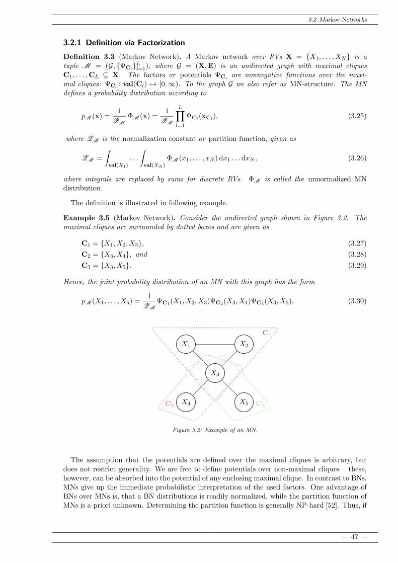
3.2 Markov Networks
3.2.1 Definition via Factorization
Definition 3.3 (Markov Network). A Markov network over RVs X = X1, . . . , XN is atuple M = (G, ΨCl
Ll=1), where G = (X,E) is an undirected graph with maximal cliquesC1, . . . ,CL ⊆ X. The factors or potentials ΨCi are nonnegative functions over the maxi-mal cliques: ΨCl
: val(Cl) 7→ [0,∞). To the graph G we also refer as MN-structure. The MNdefines a probability distribution according to
pM (x) =1
ZMΦM (x) =
1
ZM
L∏l=1
ΨCl(xCl
), (3.25)
where ZM is the normalization constant or partition function, given as
ZM =
∫val(X1)
. . .
∫val(XN )
ΦM (x1, . . . , xN ) dx1 . . . dxN , (3.26)
where integrals are replaced by sums for discrete RVs. ΦM is called the unnormalized MNdistribution.
The definition is illustrated in following example.
Example 3.5 (Markov Network). Consider the undirected graph shown in Figure 3.2. Themaximal cliques are surrounded by dotted boxes and are given as
C1 = X1, X2, X3, (3.27)
C2 = X3, X4, and (3.28)
C3 = X3, X5. (3.29)
Hence, the joint probability distribution of an MN with this graph has the form
pM (X1, . . . , X5) =1
ZMΨC1(X1, X2, X3)ΨC2(X3, X4)ΨC3(X3, X5). (3.30)
X1 X2
X3
X4 X5
C1
C2 C3
Figure 3.2: Example of an MN.
The assumption that the potentials are defined over the maximal cliques is arbitrary, butdoes not restrict generality. We are free to define potentials over non-maximal cliques – these,however, can be absorbed into the potential of any enclosing maximal clique. In contrast to BNs,MNs give up the immediate probabilistic interpretation of the used factors. One advantage ofBNs over MNs is, that a BN distributions is readily normalized, while the partition function ofMNs is a-priori unknown. Determining the partition function is generally NP-hard [52]. Thus, if
– 47 –

3 Classical Probabilistic Graphical Models
we wish to evaluate the probability of a single sample is easy in BNs, assuming that evaluationof CPDs is efficient and that the number of RVs is reasonable small. The same task can beinfeasible in MNs just by not knowing the partition function. Furthermore, as discussed in thenext section, BNs and MNs differ in the conditional independence assertions which can be readoff from their graph.
3.2.2 Conditional Independence Assertions
Similarly as in BNs, certain conditional independence assertions can be stated for MNs. To thisend, we make following definition.
Definition 3.4 (Separation). Let M be an MN over X with graph G. Two RVs Y, Y ′ ∈ X,Y 6= Y ′ are separated by Z ⊂ X, Y, Y ′ /∈ Z, if for all paths Π = (X1, . . . , Xn) between Y andY ′ there is an intermediate RV Xk ∈ Z. Two sets Y,Y′ are separated by Z ⊂ X, Y ∩ Z = ∅,Y′ ∩ Z = ∅, when all Y ∈ Y, Y ′ ∈ Y′ are separated by Z.
Theorem 3.3. Let M be an MN over X. The following conditional independence assertionshold in pM :
1. Local Markov property. A RV X is conditionally independent from all other RVs givenits neighbors, i.e.
X ⊥⊥ X \ (X ∪ nb(X)) |nb(X), (3.31)
In this context, the neighbors X are also called the Markov blanket of X.
2. Pairwise Markov property. Any two non-adjacent RVs X,Y are conditionally inde-pendent given all other RVs, i.e.
X ⊥⊥ Y |X \ X,Y , when (X − Y ) /∈ E (3.32)
3. Global Markov property. Let Y,Y′,Z ⊂ X be mutually disjoint, where Y and Y′ areseparated by Z. Then
Y ⊥⊥ Y′ |Z (3.33)
These conditional independence statements are illustrated Figure 3.3. Two simple examplesdemonstrate that the conditional independencies encoded in BNs and MNs differ from eachother:
Example 3.6 (Conditional Independencies in BNs and MNs). Consider the BN with RVs X1,X2 and X3 in Figure 3.4(a). We want to represent this BN by an MN that captures all theconditional independence properties of the BN:
• An appropriate MN must contain the edges (X1 − X3) and (X2 − X3). Otherwise, X3
would not depend on X2 and X3 as in the BN. Such an MN is shown in Figure 3.4(b). Inthis MN it holds that X2 ⊥⊥ X3 |X1, but not in the BN.
• When we additionally need to add the edge (X1 − X2) resulting in the MN shown inFigure 3.4(c). However, now the MN does in general not satisfy that X1 ⊥⊥ X2 while theBN does.
Consequently, the conditional independencies of the BN in Figure 3.4(a) cannot be representedby an MN.
– 48 –

3.2 Markov Networks
X1 X2
X3
X4 X5
(a)
X1 X2
X3
X4 X5
(b)
X1 X2
X3
X4 X5
(c)
Figure 3.3: Example for conditional independencies in MNs: (a): Local Markov property: X1 is independentfrom X4 and X5, given its Markov blanket X2, X3. (b): Pairwise Markov property: X4 andX5 are independent, given all other RVs. (c): Global Markov property: X1, X2 and X4, X5are independent given X3.
X1 X2
X3
(a)
X1 X2
X3
(b)
X1 X2
X3
(c)
Figure 3.4: Example for a BN, whose conditional independence assertions can not be represented by an MN.(a): BN to be represented as an MN. (b), (c): Candidate MNs.
– 49 –

3 Classical Probabilistic Graphical Models
Example 3.7 (Conditional Independencies in BNs and MNs). Consider the MN in Figure 3.5.We want to represent this MN by a BN capturing all the independence properties that hold inthe MN. By the pairwise Markov property we have
X1 ⊥⊥ X4 | X2, X3, and (3.34)
X2 ⊥⊥ X3 | X1, X4. (3.35)
However, these conditional independencies cannot be encoded in a BN, cf. [52].
X1 X2
X3 X4
Figure 3.5: Example for an MN, whose conditional independence assertions can not be represented by a BN.
We see that BNs and MNs do not represent the same independency assertions. Nevertheless,there exist distributions which can be represented by both MNs and BNs, as for example chainstructured models. We can visualize this situation using the notion of perfect maps (PMAPS).We call a PGM an independency map (IMAP) for a distribution p, when all conditional inde-pendence assertions represented by the graph of the PGM hold in p [52]. Conversely, we callsuch a structure a dependency map (DMAP), when when all conditional independencies of phold in the graph of the PGM. A PGM is a PMAP when it is both an IMAP and a DMAP forp. Now, consider the distributions p over a fixed set of RVs, let pB be the distributions forwhich some BN is a perfect map and pM be the distributions for which some MN is a perfectmap. The relation of p, pB and pM is symbolically illustrated by the Venn diagram inFigure 3.6, cf. [7].
p
pB pM pB ∩ pM
Figure 3.6: Venn diagram depicting the set of all probability distributions p for a fixed set of RVs, and thesets pB and pM, i.e. the distributions for which some BN or some MN is a perfect map,respectively.
3.3 Learning PGMs
After having specified BNs and MNs as models for probability distributions, we discuss how tocome up with a model for the task under consideration. One possibility is to specify a PGM byhand. Especially BNs are suited for this approach, since the directed edges can often be inter-preted as causal directions by a human domain expert. Local probability tables can be elicited
– 50 –

3.3 Learning PGMs
relatively easily using various techniques [70]. However, from machine learning perspective, wewant to automatically determine a PGM from a set of training data..
Assume we want to find a PGM for a set of random variables X which are distributed ac-cording to an unknown joint distribution p∗. Further, we have a collection of L independentand identically distributed (i.i.d.) samples D = x(1), . . . ,x(L), drawn from p∗. A natural goalof learning a PGM can be described as follows: given D, return a PGM which approximates p∗
best. This type of learning is known as generative learning, since we aim to model the processwhich generated the data. Generative learning can be seen as a “multi-purpose” tool, sincewe directly strive for the universal object describing our data: the joint distribution p∗. Otherquantities, such as marginal and conditional distributions, and expectations can in principle bederived from the joint distribution.
However, it is rarely possible to exactly retrieve p∗, especially when using a finite sample D.This can be obstructive, when the final goal is not to retrieve p∗, but to use the PGM in aspecialized way, e.g. to use the PGM as classifier. In the classification context we are primarilyinterested in minimizing the loss resulting from erroneous decisions, not in modeling the overallgenerative process. It can be easily shown that knowledge of p∗ leads to optimal classification,and therefore generative learning seems to be suitable to learn classifiers. However, a consistentobservation in machine learning is that discriminative learning methods, which refrain frommodeling p∗, but directly address the classification problem, often yield better classificationresults than the generative approach.
Furthermore, there are two key aspects of learning a PGM: the structure G and the CPDs orclique factors, which we assume to be represented by a parameter set Θ. Although G and Θ arecoupled, e.g. the number of parameters depends on G, an isolated consideration of G and Θ isoften reasonable. This leads to the two tasks of learning PGMs: parameter learning and struc-ture learning. Thus, we can consider many kinds of learning approaches: generative/discrim-inative parameter learning, generative/discriminative structure learning, combinations thereof,e.g. learning structure discriminatively and learning parameters generatively. Furthermore, thereexist hybrid approaches, e.g. hybrid generative-discriminative learning objectives. More infor-mation about discriminative/hybrid learning can be found in [52,71,77]. In this thesis, however,we focus on the generative approach.
Let us assume a specific class of models C, e.g. the class of all BNs, or the class of all MNs.Following a Bayesian approach to learning, we define a prior distribution p(C) over the modelclass, which represents our preference for certain models. For example, if C is the class of allBNs, we may prefer networks with fewer edges, and therefore define a prior which decreases withthe number of edges. We are interested in the posterior probability distribution over the modelclass, conditioned on the given data. Using Bayes’ law, this distribution is
p(C |D) =p(D | C) p(C)
p(D)=
p(D | C) p(C)∫C p(D |M ′) p(M ′) dM ′
∝ p(D | C) p(C). (3.36)
The data generation probability p(D | C) is known as likelihood L(C;D).
There exist two main approaches to use the posterior distribution:
1. Maximum a-posteriori (MAP) approach. This approach aims to find the most prob-able model MMAP ∈ C for given data, i.e.
MMAP = arg maxM∈C
p(M | D) (3.37)
= arg maxM∈C
L(M ;D) p(M). (3.38)
In the MAP approach we accept the single model MMAP as best explanation for the dataand use it for further tasks.
– 51 –

3 Classical Probabilistic Graphical Models
2. Bayesian model averaging. In model averaging, we refrain to decide for a single modelout of C. Instead, we maintain the uncertainty about which model might be the “true”one and keep the whole model class C, together with the posterior distribution p(C |D).
As an illustrating example, consider the probability of an unseen sample x′, after observing D.The MAP approach dictates that
p(x′ | D) = p(x′ |MMAP), (3.39)
while the model averaging approach results in
p(x′ | D) =
∫Cp(x′ |M) p(M | D) dM. (3.40)
Model averaging proceeds more carefully and treats the uncertainty by marginalizing over allpossible models. They often agree in the large sample limit, since for large L the mass of theposterior p(C |D) is typically concentrated on a single model. For small sample sizes, modelaveraging often outperforms the MAP approach.
Parameter Learning
For parameter learning, we assume that the network structure G is fixed, maybe because adomain expert specified the independence relationships among the model variables, or becausea structure learning algorithm already provided an appropriate structure. Therefore, for pureparameter learning, the model class C is represented by parameters Θ. In the special casewhen the prior distribution p(Θ) is flat, i.e. no model is preferred over the other, the posteriorp(Θ | D) is proportional to the likelihood L(Θ;D), and the MAP solution coincides with theclassical maximum-likelihood (ML) solution, i.e.
MMAP = MML = arg maxM∈Θ
L(M ;D). (3.41)
When the data samples D are i.i.d., the likelihood is given as
L(Θ;D) = p(D |Θ) =L∏l=1
p(x(l) |Θ). (3.42)
It is usually more convenient to work with the log-likelihood
logL(Θ;D) =L∑l=1
log p(x(l) |Θ). (3.43)
Maximizing log-likelihood is equivalent to maximizing likelihood. Intuitively, the log-likelihoodis a measure of goodness of fit, i.e. a model with maximum likelihood is considered as bestexplanation for the training data. Furthermore, maximizing likelihood yields under rather mildassumptions a consistent estimator of the model parameters, i.e. if p∗ lies in our model class, itsparameters are recovered in the large sample limit.
Consider first the class of BNs. For parameter learning with fixed BN structure G andi.i.d. samples D = x(1), . . . ,x(L), the log-likelihood of a BN model is given as
logL(B;D) =L∑l=1
∑X∈X
log p(x(l)X |x
(l)pa(X);θ
X) =∑X∈X
`(θX ;D). (3.44)
We see that the log-likelihood decomposes into a sum over local terms, one for each RV X, given
– 52 –

3.3 Learning PGMs
as
`(θX ,D) =
L∑l=1
log p(x(l)X |x
(l)pa(X);θ
X). (3.45)
Therefore, the overall BN log-likelihood is maximized by maximizing the individual local termsw.r.t. the local parameters θX .
This decomposition property simplifies generative learning in BNs and often leads to closedform solutions. In the case of finite-state RVs, see Example 3.3, the ML parameters are givenby [77]:
θXx|xpa=
∑Ll=1 1(x
(l)X = x ∧ x
(l)pa(X) = xpa)∑
x′∈val(X)
∑Ll=1 1(x
(l)X = x′ ∧ x
(l)pa(X) = xpa)
=nXx|xpa∑
x′∈val(X) nXx′|xpa
, (3.46)
where the data counts nXx|xpa=∑L
l=1 1(x(l)X = x ∧ x
(l)pa(X) = xpa) are the sufficient statistics for
this problem. When nXx′|xpa= 0 for all x′, the solution in (3.46) is not defined. In this case,
however, any arbitrary CPT for the particular X and xpa is an optimal solution. In practice,one often uses smoothed ML parameters, i.e. a small constant is added to each nXx′|xpa
.
Finding ML parameters for MNs is typically harder than for BNs, and usually no closed formsolution exists. When the clique factors are assumed to be log-linear, i.e.
ΨCl= exp(θl fl(Cl)), (3.47)
where fl(Cl)) is an arbitrary feature function, then the log-likelihood is concave. In this case,an ML solution can be found using convex optimization, e.g. gradient methods. However,this requires computing the partition function in each iteration, which renders ML-parameterlearning in MNs generally NP-hard [52].
So far, we assumed complete data, i.e. all values in a sample x are available. However, missingdata scenarios are common in machine learning, where possible reasons for missing data are:
• We fail to record the values of all RVs, e.g. because of corrupted measurements.
• We have latent RVs in our model, because they are justified from our domain knowledge,but they can not be directly observed.
• We introduce latent RVs in our model, as a modeling technique per se. For example, in aBayesian approach, we introduce the model parameters explicitly in the model as additionalRVs. As another example, mixture model are often interpreted as an augmented modelwhere a hypothetical latent RVs is marginalized.
Although reasons for missing data might be various, its treatment is consistent in the probabilis-tic framework, using the expectation-maximization (EM) algorithm [30,65]. Let Y(l) be the setof observed RVs in the lth sample, y(l) the corresponding observed value, and Z(l) = X \Y(l).One step of the EM algorithm is given as
Θt+1 = arg maxΘ
Q(Θ,Θt), (3.48)
Q(Θ,Θt) =L∑l=1
∑z(l)∈val(Z(l))
p(z(l) | y(l); Θt) log p(z(l),y(l); Θ). (3.49)
Q is the expected data likelihood of Θ, where the expectation is taken with respect to the currentparameters Θt, and has the natural interpretation of probabilistic data completion. In BNs over
– 53 –

3 Classical Probabilistic Graphical Models
finite-state RVs the EM algorithm takes a particular intuitive form [52]: In a first step, theso-called E-step, we compute the expected sufficient statistics:
nXx|xpa=
L∑1=l
pB(X,paX |y(l); Θt). (3.50)
In the so-called M-step we treat the expected sufficient statistics as if they were actual sufficientstatistic, yielding parameter updates as in (3.46), using nXx|xpa
instead of nXx|xpa. This approach
generally carries over to BNs with CPDs from the exponential family [52]. The EM algorithmfor MNs is generally less appealing, since we generally lack of closed form ML solutions for theclique factors.
Structure Learning
There exist two main approaches to structure learning in PGMs:
1. Constraint-based approaches. In this approach, one aims to find a structure G whichrepresents the same conditional independencies as present in the underlying distribution ofdata. Although theoretically sound, these methods rely on statistical independence testsperformed on the data, which are usually too inaccurate in practice. Further informationabout this approach can be found in [52,91,99].
2. Scoring-based approach. Here one aims to find a graph which represents a suitabledistribution to represent the true distribution p∗, where suitability is measured by a scoringfunction score(G). There are two key issues here: Defining an appropriate scoring function,and developing a search algorithm which finds a score-maximizing structure G.
A first choice for the scoring function would be the log-likelihood, i.e. to find the structure Gwhich, when equipped with ML parameters, maximizes the log-likelihood. However, it easy tosee that a fully connected graph will always be a maximizer of the log-log-likelihood, leading tooverfitting. As a remedy, one modifies the pure likelihood-score in order to account for modelcomplexity. One approach is the minimum description length (MDL) principle [82], which aimsto find the shortest, most compact representation of the data D within the considered modelclass. The MDL principle additionally accounts for the description length of the model, whichis measured by the number of parameters. For example, the MDL score for BNs with discretevariables was derived as [55,94]:
MDL(G) = −L∑l=1
log p(x(l) | G,ΘML) +logL
2T (G), (3.51)
where T (G) is the number of free parameters Θ. We want to minimize MDL, thus it is actuallya negative score.
An alternative way to avoid overfitting is delivered by a Bayesian approach. The main problemwith the likelihood as score is that it is not aware of model complexity, i.e. the number of freeparameters. While with more densely connected graphs G the dimensionality of the parameterspace Θ increases exponentially, nevertheless only a single point estimate is used from this space,i.e. the ML parameters ΘML. Therefore, the ML approach can be described as overly optimistic,trusting in the single “true” parameters ΘML. In contrast to the ML approach, the Bayesianapproach uses the parameter space in its entirety. Introducing a prior distribution p(Θ) and
– 54 –

3.3 Learning PGMs
marginalizing over Θ, leads to the Bayesian score (cf. [77]):
Bayes(G) = p(D|G) =
∫Θp(D|Θ,G) p(Θ) dΘ (3.52)
=
∫Θ
L∏l=1
p(x(l)|Θ,G) p(Θ) dΘ. (3.53)
For BNs over finite-state RVs, using Dirichlet priors for the local parameters leads under rathermild assumptions to the closed form Bayesian-Dirichlet score (BD) [11, 22, 44]. For undirectedmodels, the Bayesian score is usually not feasible. The large sample limit of the BD score isknown as Bayesian information criterion (BIC) and is equivalent to MDL. BIC can also definedfor MNs and takes the same form as (3.51).
A common approach for MNs is to formulate structure learning as parameter learning problem.The most prominent score is `1-penalized likelihood:
L1(Θ) =L∑l=1
log p(x(l) | G,ΘML)− λ ‖Θ‖1. (3.54)
This approach is actually a hybrid of parameter and structure learning: a general structureG is hold fixed, where minimization of ‖Θ‖1 leads to an effective sparsification of the graph,determining the effective structure.
In BNs, pure structure learning is often considered, especially when closed form parametersare available. Having chosen an appropriate scoring function, how do we find a graph G whichmaximizing it? Explicit enumeration of all DAGs is clearly infeasible, since the number of DAGsgrows super-exponentially with the number of nodes [83]. All the scores discussed so far, namelylog-likelihood, MDL and BIC, and (the logarithm of) the BD/BDe score can be written in theform
score(G;D) =∑X∈X
scoreX(pa(X);D), (3.55)
which means that the global network score decomposes into a sum of local scores, dependingonly on the set of parents for each RV. This property helps to improve the efficiency structurelearning algorithms. Nevertheless, the problem of finding a score-maximizing BN structure Gis NP-hard in general, even when using decomposable scores and even when the maximumnumber of parents is restricted to K ≥ 2 [15, 17]. For K = 1, i.e. when the BN is restricted toa directed tree (or actually a directed forest), the Chow-Liu algorithm [20] learns an optimalnetwork structure in polynomial time, maximizing the log-likelihood over the class of BNs witha directed tree structure. The class of directed trees is typically restrictive enough to avoidoverfitting, i.e. the likelihood score is an appropriate choice in this case.
For learning more complicated structures, there exist a variety of approximative techniques.One of the first general search algorithms was the K2 algorithm [22] which relies on an initialvariable ordering, and greedily adds parents for each node, in order to increase the BD score.A more general scheme is greedy hill-climbing (GHC) [18,44], which does not rely on an initialvariable ordering. In each GHC iteration, the current graph candidate G is replaced with aneighboring graph G′ when score(G′) > score(G), where neighboring graphs are resulting fromthe current graph when applying certain graph transformations, e.g. single edge-insertions, edge-deletions and edge-reversals. GHC can be combined with tabu-search [41] in order to escapelocal maxima in the search space. A further method is simulated annealing (SA) which randomlygenerates a neighbor solution in each step; If the new solution has higher score than the currentone, it is immediately accepted, while a solution with lower score is accepted with a certainprobability. While this probability is high in the beginning, leading to a large exploration over
– 55 –

3 Classical Probabilistic Graphical Models
the search space, it is successively reduced according to a cooling schedule. Other approachesconsider other search spaces than the space of all DAGs: In [16] it is proposed to search over thespace of equivalence classes, i.e. classes of BN structures which represent the same independenceassertions. In [96], a search over possible variable orderings is proposed. This approach uses thefact, as already mentioned in [22], that for a given variable ordering the optimal structure canbe found in polynomial time.
There exist also exact approaches, globally optimizing the BN structure. Methods basedon dynamic programming [51, 88, 89] have exponential time and memory requirements, whichrestricts their application to approximately 30 variables. Furthermore, there are branch-and-bound methods [28,45,95] which cast the combinatorial structure learning problem to a relaxedcontinuous problem. Although branch-and-bound methods also have exponential run-time, theyprovide two key advantages: (i) They maintain (after some initial time) a feasible solution,i.e. they can be prematurely terminated, returning the currently best solution. (ii) They provideupper and lower bounds on the maximal score, which represents a worst-case certificate of sub-optimality. Exact methods can also be applied in the discriminative case [76].
3.4 Inference in PGMs
In the last sections we introduced the BNs and MNs as probabilistic models and discussedlearning approaches to fit a PGM to given data. To process of performing reasoning with aPGM, i.e. to answer queries using our model, is generally called inference. Assume that p is ourmodel distribution over RVs X. Common inference scenarios are:
1. Marginalization. We wish to obtain the marginal distribution p(Xq) for some subset ofquery RVs Xq ⊂ X, marginalizing X \Xq = Xm = Xm
1 , . . . , XmK , i.e. compute
p(Xq) =
∫val(Xm
1 ). . .
∫val(Xm
K )p(Xq, xm1 , . . . , x
mK) dxm1 . . . dxmK . (3.56)
In the case of discrete RVs, the integrals are replaced by sums.
2. Conditionals. Here X is split into disjoint query RVs Xq, observed RVs Xo and marginal-ized RVs Xm. The goal is to find the posterior distribution of the query variables Xq
conditioned on the observation xo, i.e. compute
p(Xq |xo) =p(Xq,xo)
p(xo)(3.57)
The terms p(Xq,xo) and p(xo) are determined by marginalization over Xm and Xm ∪Xq.
3. Most probable explanation. (MPE) Here X is split into query RVs Xq and observedRVs Xo. The goal is to find the most probable explanation (MPE) for Xq, i.e. find
xq∗ = arg maxxq∈val(Xq)
p(xq |xo) = arg maxxq∈val(Xq)
p(xq,xo) (3.58)
4. Maximum a-posteriori. (MAP) Here X is split into query RVs Xq, observed RVs Xo
and marginalized RVs Xm = Xm1 , . . . , X
mK . Similar as MPE we aim to find the most
– 56 –

3.4 Inference in PGMs
probable explanation for Xq given Xo, but additionally ignore Xm, i.e. compute
xq∗ = arg maxxq∈val(Xq)
p(xq |xo) (3.59)
= arg maxxq∈val(Xq)
p(xq,xo) (3.60)
= arg maxxq∈val(Xq)
∫val(Xm
1 ). . .
∫val(Xm
K )p(xq,xo, xm1 , . . . , x
mK) dxm1 . . . dxmK . (3.61)
Unfortunately, all these inference scenarios are NP-hard in general [52]. Furthermore, MAP isinherently harder than MPE [8, 68, 69]. However, the essential aim of PGMs is to target atmodels which allow tractable inference. To this end one aims to design inference algorithmswhose computational cost adapts to the complexity of the PGMs. An alternative approach isto give up the aim to solve an inference scenario exactly, and to resort to approximate inferencemethods.
Exact inference methods aim to use the factorization properties of the PGM at hand. Inthe case of BNs, common practice is to first transform the BN into a MN by a process calledmoralization: Any two parent of an RV are connected by an undirected edge, any directed edgeis replaced by an undirected one and the CPDs of BNs are interpreted as clique potentials. Theresulting MN then represents the same distribution as the BN, i.e. it is an IMAP for the BN,but obscures the typical ’explaining away’ independence assertion in BNs, see also Example 3.6.An example of the moralization process is shown in Figure 3.7 (b). In this way, one can treatgeneral purpose inference for BNs and MNs in a common framework. The basic observationis that marginalization and maximization in tree-shaped MNs can be solved efficiently, leadingto a message passing scheme called belief-propagation [7, 62, 70]. The main idea is now togeneralize this positive result to more general graphs, by transforming them into tree shapedmodels by clustering together RVs. The way this is achieved is by finding a so-called junctiontree or clique tree, where each node in the tree corresponds to a clique in the original model[23, 24, 49, 58]. In order to yield consistent results, a junction tree has to fulfill the so-calledrunning intersection property, meaning that when an RV is contained in two different cliques Ci
and Cj , then it must also be contained in each clique on the path connecting these two cliques.Such a clique tree does not necessarily exist for arbitrary graphs. However, it always existfor chordal graphs. So we can introduce additional edges until the graph is chordal, a processcalled triangulation. This effectively removes independence assertions from the model. A simpleway to find a triangulation found is by the elimination algorithm [52]. Inference cost in theresulting junction tree is exponential in the size of the largest clique in the used chordal graph,thus we wish to find a triangulation which minimizes the maximal clique size. This problem,unfortunately, is NP hard, requiring heuristics to find triangulated graphs with reasonable smallcliques. Finally, a junction tree can be generated from the triangulated graph, by finding themaximal cliques and the connections [52]. A junction tree of the example in Figure 3.7 is shownin Figure 3.8.
Exact inference using belief propagation on junction trees is feasible only for PGM whosegraphs are not too densely connected. There are various approximate inference methods, suchas variational methods, loopy belief propagation and sampling methods [52, 77].
– 57 –

3 Classical Probabilistic Graphical Models
X1
X2 X3
X4 X5
X6
(a)
X1
X2 X3
X4 X5
X6
(b)
X1
X2 X3
X4 X5
X6
(c)
Figure 3.7: Example of moralization and triangulation. (a): BN to be moralized. (b): Moralized graph,yielding a MN; directed edge are replaced by undirected ones and an undirected edge is insertedbetween X4 and X5, which are co-parents of X6. (c): Triangulated graph.
X1, X2, X3 X2, X3 X2, X3, X4
X3, X4
X4, X5, X6 X4, X5 X3, X4, X5
Figure 3.8: Example junction tree for the example in Figure 3.7.
– 58 –

Foundations of Sum-Product Networks for Probabilistic Modeling
4Sum-Product Networks
Parts of this chapter are published in [75]. Similar as classic PGMs, SPNs are a graphicaldescription of probability distributions – their syntax and semantics, however, differ largelyfrom BNs and MNs. Before we introduce SPNs, let us point out to some weak points of classicPGMs which call for an alternative model type.
In classic PGMs, the process of learning and inference is traditionally treated in a decoupledway. This separation is somewhat artificial and myopic, since inference is often a sub-processof learning. Thus, models in which exact inference is intractable can often also not be properlylearned. Sometimes one seeks to solve these issues using approximate inference for learning.This approach has several drawbacks:
• We do not know which approximate inference method will work for our task at hand.Trying out and cross-tuning several approximate inference methods is tedious work.
• Using an approximate inference method in a correct learning algorithm can yield unpre-dictable results. Correctness of learning is sometimes not guaranteed, when approximateinference is used.
• Approximate inference, such as sampling methods, often trade off computation time andaccuracy. Finding a good trade-off for a problem at hand is usually difficult. This is alsoa problem in the actual inference stage.
Thus, if we want to avoid these difficulties about approximate inference, we are forced to usemodels in which exact inference is tractable. However, this approach will generally restrict us tosparsely connected and usually overly simplistic PGMs. In this context, PGMs appear somewhatbulky and counterintuitive from a modeler’s perspective, since a model might be easily renderedintractable, just by adding a single, seemingly harmless edge.
This suggest that the conditional independence assertions in BNs and MNs are too coarse inpractice, meaning that in many cases we do not want to consider conditional independencieslike
Y ⊥⊥ Y′ |X (4.1)
but also context-specific independencies (CSI) like
Y ⊥⊥ Y′ |X = x, (4.2)
– 59 –

4 Sum-Product Networks
i.e. when independence between Y and Y′ hold just for certain values of X, but not for allvalues. This approach is not new and several learning algorithms exploiting CSI were proposed,see for instance [10, 19]. However, CSI can not be captured in the overall DAG, but has to beencoded in the CPDs. For instance, this can done using default tables or decision trees, leadingto a intransparent, nested model. These models also need specialized inference algorithms.
A simple and often used technique to design models which exhibit little or no conditional in-dependencies among the modeled RVs X, is to use mixtures of distributions. Mixtures of distri-butions can be interpreted as augmenting the set of RVs by a latent RV Z which is marginalized.This principle can be extended to multiple, hierarchically organized latent RVs, see for instancethe work in [34–37,56,57,102,103].
SPNs, are a type of probabilistic model which addresses these points. In their basic description,SPNs are simply networks of sum and product operations with certain numeric inputs. Thus,they can be interpreted as a potentially deep neural network with two types of neurons: sumsand products. SPNs in the form as discussed in this thesis admit following features:
• SPNs represent probability distributions over RVs X.
• Many inference scenarios are stated as conceptional simple and easily implementable net-work evaluations.
• The computational cost of these inference scenarios scales linearly with the network size.
• SPNs can be interpreted as potentially deep and hierarchical structured latent RV model.
Although SPNs have been discussed in literature for some while, some aspects are not yet wellunderstood. The main goal of this thesis is to revisit the theoretic foundations and to gain adeeper understanding about SPNs. In Section 4.2 we review an important tool related to SPNs:the network polynomial. We introduce SPNs over finite-state RVs in Section 4.3 and generalizethem to discrete RVs with infinitely many states and to continuous RVs in Section 4.4. Beforewe start, it will be helpful to introduce some notation about representing evidence.
4.1 Representing Evidence
For a given set of RVs X, the elements of x ∈ val(X) can be interpreted as complete evidence,assigning each RV in X a value. Given a distribution p over X, a typical task is to evaluate thedistribution for this evidence, i.e. compute p(x).
Now assume that for a subset Y ⊂ X we have complete evidence y available. For evaluatingthe probability of this evidence, we need to marginalize Z = X \ Y. This can be interpretedthat we have partial evidence for each Z ∈ Z, namely that
Z(ω) ∈ val(Z) (4.3)
This is of course an extreme case of “evidence”, stating that Z assumes a value in val(Z), i.e. thatwe have no evidence about Z at all. However, this can be generalized to partial evidence that
Z(ω) ∈ Z, where Z ⊆ val(Z). (4.4)
To avoid problems with non-measurable sets we require Z ∈ AZ := B(val(Z)), i.e. the Borelsets over val(Z), cf. Section 2.1. Recall that for countable val(Z), we have AZ = 2val(Z). Weuse calligraphic letters to denote partial evidence, i.e. X ,Y,Z is partial evidence for X,Y, Z,respectively. To represent partial evidence about sets of RVs X = X1, . . . , XN, we use the
– 60 –

4.2 Network Polynomials
product sets
HX :=
N
ą
n=1
Xn | Xn ∈ AXn
. (4.5)
Elements of HX,HY,HZ are denoted as X , Y , Z, respectively. When Y ⊆ X, Y ∈ X andX ∈ HX, we define X [Y] := x[Y] | x ∈ X and X [Y ] = x[Y ] | x ∈ X.
Given a distribution p over X = X1, . . . , XN, a typical task is to compute the probabilityof partial evidence X , i.e. compute
P (X ) =
∫X [X1]
. . .
∫X [XN ]
p(x1, . . . , xN ) dx1 . . . dxN =:
∫Xp(x) dx, (4.6)
where the vector-style integral on the right-hand side of (4.6) is a shorthand. For discrete RVs,these integrals are replaced by sums. When working with both discrete and continuous RVs, wewill always use integrals as in (4.6) for notational simplicity, without explicitly mentioning thatthey have to be replaced by sums for discrete RVs.
The most general representation of evidence used in this thesis is that X is split into disjointY,Y′, where for Y′ we have complete evidence y′ and for Y we have partial evidence Y . Thiscovers several types of evidence and inference scenarios:
• Y = ∅: Evaluate complete evidence p(x) = p(y′).
• Y′ = ∅: Evaluate partial evidence P (X ) =∫X p(x) dx =
∫Y p(y) dy.
• Y 6= ∅, Y′ 6= ∅: Evaluate evidence∫Y p(y,y
′) dy = p(y′ |Y)P (Y ∈ Y).
These types of evidence and inference scenarios also cover cases when Y ∪Y′ ⊂ X, i.e. whenevidence does not include all RVs in X and we marginalize X \ Y ∪ Y′. As already pointedout in (4.3), this is just a special case of partial evidence and we simply add Z = X \ (Y ∪Y′)to Y with partial evidence Y [Z] = val(Z). Note that for discrete RVs it suffices to considerpartial evidence only, since when all X [X] = x are singletons, then P (X ) = p(x), where xis composed of the singletons. When working with continuous RVs, we need to consider bothcomplete and partial evidence: complete evidence corresponds to evaluating a PDF, while partialevidence corresponds to integration.
4.2 Network Polynomials
In this section we review the notion of network polynomials, a description of distributions overfinite-state RVs. Network polynomials were introduced in [27] for BNs, and generalized toarbitrary unnormalized distributions in [79]. Marginalization using network polynomials canbe compactly expressed by setting indicator variables corresponding to the RVs states. Thederivatives of the network polynomial deliver certain probabilistic interpretations, which is calledthe differential approach to inference.
4.2.1 Representation of Distributions as Network Polynomials
Let X be a set of finite-state RVs. For each RV X and each state x ∈ val(X), we introduce anindicator variable (IV) λX=x ∈ R. The vector containing all IVs is denoted as λ. Darwiche [27]defines the network polynomial as a function corresponding to a BN B over X. Recall that B
– 61 –

4 Sum-Product Networks
defines the probability distribution (cf. Example 3.3)
pB(x) =∏X∈X
θXx[X],x[pa(X)]. (4.7)
The network polynomial of a BN is a multi-linear function of λ defined as follows.
Definition 4.1 (Network polynomial of a Bayesian network). Let B be a BN over finite-stateRVs X. The network polynomial fB of B is defined as
fB(λ) =∑
x∈val(X)
∏X∈X
λX=x[X] θXx[X],x[pa(X)]. (4.8)
As shown in [27], the network polynomial represents the BN distribution in the followingsense. Let us restrict λX=x to values 0, 1 and define them as function of x ∈ val(X):
λX=x(x) =
1 if x[X] = x
0 otherwise.(4.9)
Let λ(x) be the corresponding vector-valued function, containing all λX=x(x). This λ(x) rep-resents a 1-of-K coding of x. Clearly, the image of function λ(x) is not the set of all binaryvectors, i.e. there are “invalid” binary vectors not representing some x. When we input λ(x) tothe network polynomial, all but one of the exponentially many terms in the sum in (4.8) vanishand we have
fB(λ(x)) =∏X∈X
θXx[X],x[pa(X)] = pB(x), (4.10)
At a first view, the representation of the BN distribution as network polynomial seems cumber-some and not very useful. However, the network polynomial allows us to perform marginalizationover partial evidence in a compact way. To this end, let us generalize function (4.9) to the domainHX. For any X ∈ HX, let
λX=x(X ) =
1 if x ∈ X [X]
0 otherwise.(4.11)
Let λ(X ) be the corresponding vector-valued function, containing all λX=x(X ). In contrast toλ(x), the function λ(X ) maps to all binary vectors and is invertible. That is, λ(X ) uniquelyencodes the elements of HX. When we input λ(X ) to the network polynomial, it evaluates to
fB(λ(X )) =∑x∈X
∏X∈X
θXx[X],x[pa(X)] =∑x∈X
pB(x) = PB (X ) . (4.12)
The network polynomial marginalizes over partial evidence, by simply setting the correspondingIVs to 1. In other words, when plugging in (4.11), the network polynomial evaluates the prob-ability measure on HX. We use the shorthands fB(x) and fB(X ) for fB(λ(x)) and fB(λ(X )),respectively. The notion of the network polynomial can be easily generalized to arbitrary un-normalized distributions, as done in [79]:
Definition 4.2 (Network Polynomial of Unnormalized Distributions). Let Φ be an unnormalizedprobability distribution over discrete RVs X, i.e. ∀x ∈ val(X) : Φ(x) ≥ 0, ∃x ∈ val(X) : Φ(x) >0. The network polynomial fΦ of Φ is defined as
fΦ(λ) =∑
x∈val(X)
Φ(x)∏X∈X
λX=x[X]. (4.13)
– 62 –
4.2 Network Polynomials
The network polynomial according to Definition 4.2 subsumes the one according to Defini-tion 4.1, by setting Φ ≡ pB. Similar as for fB, we have for x ∈ val(X)
fΦ(λ(x)) = Φ(x), (4.14)
and for X ∈ HX
fΦ(λ(X )) =∑x∈X
Φ(x). (4.15)
Note that when λ ≡ 1, fΦ(λ) returns the normalization constant of Φ. We define fΦ(x) :=fΦ(λ(x)) and fΦ(X ) := fΦ(λ(X )).
Besides compactly describing marginalization, the network polynomial can be used in theso-called differential approach to inference, described in the next section.
4.2.2 Derivatives of the Network Polynomial
First let us consider the derivatives with respect to some IV. The network polynomial (4.13) isan exponential sum over terms
tx(λ) = Φ(x)∏X∈X
λX=x[X]. (4.16)
The derivative of tx(λ) is
∂tx(λ)
∂λX=x=
Φ(x)
∏X′∈X\X λX′=x[X′] if x[X] = x
0 otherwise.(4.17)
The derivative of the network polynomial is the sum over the derivatives of the form (4.17),which equals the evaluation of fΦ at a modified IV vector λ′:
∂fΦ
∂λX=x(λ) = fΦ(λ′), where (4.18)
λ′Y=y =
λY=y if Y 6= X
1 if Y = X, y = x
0 if Y = X, y 6= x
(4.19)
For X ∈ HX, the derivative of the network polynomial equals
∂fΦ
∂λX=x(λ(X )) =
∑x′∈X [X\X]
Φ(x,x′). (4.20)
i.e. the derivatives with respect to the IVs yield evaluations for modified evidence, replacingX [X] by x. In particular, for any x ∈ val(X), we have
∂fΦ
∂λX=x(λ(x)) = Φ(x,x[X \ X]), (4.21)
Using these derivatives, we obtain the conditional probabilities of the form
Φ(x |X [X \ X]) ∝ ∂fΦ
∂λX=x(λ(X )). (4.22)
– 63 –

4 Sum-Product Networks
These conditional distributions, to which we refer as marginal posteriors, are for instance usefulfor approximate MAP solvers [68, 69]. Higher order derivatives with respect to the IVs havesimilar semantics, e.g. for the second order derivative we have
∂2fΦ
∂λX=x∂λY=y(λ(X )) =
∑x′∈X [X\X,Y ] Φ (x, y,x′) if X 6= Y
0 otherwise.(4.23)
For network polynomials of BNs (Definition 4.1), the derivatives with respect to the networkparameters also have a probabilistic interpretation [27]. Derivatives with respect to the networkparameters can further be used for learning BN parameters, using gradient techniques. Fur-thermore, they are important for sensitivity analysis [12, 13] and for learning BNs with certainparameter constraints, such as reduced numeric precision [97].
4.2.3 Arithmetic Circuits
A direct implementation of network polynomials in the form (4.13) is not practical, due to itsexponentially many summation terms, and one strives for a more compact representation. Oneapproach uses arithmetic circuits [26, 27].
Definition 4.3 (Arithmetic circuit). An arithmetic circuit (AC) is a rooted acyclic directedgraph, whose leaves are numeric inputs and whose internal nodes are arithmetic operations (+,−, ×, ÷) of its children. The output of the AC is the value computed by its root. The size ofthe AC is the number of its edges.
The size of the AC reflects the computational cost of evaluation, since each edge correspondsto exactly one arithmetic operation. While in general ACs can represent arbitrary arithmeticfunctions, the focus in [26, 27] lies on representing the network polynomial fB of some BN asa compact AC. The leaves of the AC are used to represent parameters and IVs of the networkpolynomial, and the arithmetic operations are restricted to additions and multiplications. Itis pointed out that the junction tree algorithm can be interpreted as one particular choice forcompiling a BN to an AC. This work further proposes to represent BNs via logical theories whichin turn can be compiled to ACs. The approach in [64] goes one step further and directly learnsan AC optimizing a scoring function, trading off the training likelihood, number of parameters,and inference complexity in terms of AC size. Basically, this algorithm learns a BN with context-specific independencies [19], where CPTs are organized as decision trees [19]. In [63], an ACis learned by optimizing a trade-off of likelihood and number of parameters, where the ACrepresents a Markov network over discrete variables. This method starts with an AC consisting ofa product over all single variable features and iteratively introduces new features by conditioningan existing feature on all values of a “splitting” variable. For both methods [63, 64] the log-likelihood is concave in the model parameters, i.e. a global maximum likelihood solution isobtained.
Since these ACs represent a network polynomial, they can be used for efficient evaluation ofany X ∈ HX using a single upwards-pass in the network. Therefore, inference cost is directlyrelated with the size of the AC. Furthermore, following the differential approach, one can obtainthe first-order derivatives of IVs and network parameters. Differentiating a given AC can be doneby back-propagation, where a single back-propagation pass delivers simultaneously all derivativeswith respect to IVs and parameter nodes [27].
SPNs, introduced in the next section, are actually a special type of ACs, restricted to weightedsum and product operations. The weighted sums can actually be implemented by a productoperation and an additional numeric input. Therefore, SPNs are not a “more powerful” com-putation architecture than ACs – in fact they can be seen as a subset of ACs – however, theprobabilistic interpretation of SPNs are defined in a more direct manner.
– 64 –

4.3 Finite-State Sum-Product Networks
4.3 Finite-State Sum-Product Networks
We start with the definition of SPNs as presented in [79], which represent probability distribu-tions over finite-state RVs. We generalize SPNs to RVs with countably infinitely many statesand continuous RVs in Section 4.4.
Definition 4.4 (Finite-State Sum-Product Network). A sum-product network S = (G,w)over finite-state RVs X = X1, . . . , XN is a rooted acyclic directed graph G = (V,E) and a setof nonnegative parameters w. The nodes V ∈ V are functions mapping λ to R. There are threetypes of nodes:
1. Indicators: λX=x
2. Sums:
S(λ) =∑
C∈ch(S)
wS,C C(λ), (4.24)
where the weight wS,C ∈ w is associated with edge (S→ C) ∈ E.
3. Products:
P(λ) =∏
C∈ch(P)
C(λ). (4.25)
All leaves of G are IVs and all internal nodes are either sums or products. w is the set of allweights associated with sum nodes. The function computed by S is the function computed by theroot and denoted as S(λ).
We denote nodes of SPNs with λ, S, P, N, C, F where we use the following rules to easediscussion. N denotes a general SPN node without specifying its type, i.e. whether it is an IVs,a sum or a product. C and F are also general nodes, but are used to highlight their role asas children and parents of other nodes, respectively. For IVs, sums and products, we use thesymbols λ, S and P, respectively. The set of all sum nodes and product nodes of an SPN S aredenoted as S(S) and P(S), respectively. Similarly, λ(S), λX(S) denote the set of all IVs andthe set of all IVs related to X, respectively.
The functions which can be computed or represented by SPNs are the polynomials in λ, withnonnegative coefficients and without constant term, i.e. any SPN S computes a polynomial ofthe form ∑
i
αi∏
λ∈λ(S)
λkλ,i , where
∀i :∑
λ∈λ(S)
kλ,i ≥ 1, kλ,i ∈ N0, αi ≥ 0.(4.26)
Conversely, for any function of this form we can easily find an SPN computing it. In particular,any network polynomial (4.13) has this form, i.e. any network polynomial can be represented bysome SPN. For a trivial representation of a network polynomial we can use a single sum with|val(X)| products (monomials)
∏X∈X λX=x[X] as children and having Φ(x) as weights. This
representation is a shallow SPN. A point of major interest is to represent network polynomialsmore compactly, using deep architectures. Similar as for network polynomials, we can plug in
– 65 –

4 Sum-Product Networks
the functions λ(x) and λ(X ) from (4.9) and (4.11) and define
N(x) := N(λ(x)) (4.27)
N(X ) := N(λ(X ) (4.28)
S(x) := S(λ(x)) (4.29)
S(X ) := S(λ(X )). (4.30)
The number of addition operations of an SPN S is AS :=∑
S∈S(S) |ch(S)| = |w| and thenumber of multiplication operations is MS :=
∑P∈P(S)(|ch(P)| − 1) + |w|. AS and MS are the
worst-case number of required arithmetic operations to evaluate S(λ); when some wS,C or someλX=x equal zero, evaluation of S(λ) can be cheaper.
We introduce the notion of the scope of SPN nodes.
Definition 4.5 (Scope of SPN Node). Let S be an SPN over RVs X and N be some node in S.The scope of N, denoted as sc(N), is defined as
sc(N) =
X if N is some IV λX=x⋃
C∈ch(N) sc(C) otherwise(4.31)
To avoid pathological cases, we assume that for each N there exists x ∈ val(X) such thatN(x) > 0. It is easily shown that this is equivalent to the condition that each sum node has atleast one strictly positive weight. We now define the distribution of an SPN.
Definition 4.6 (Distribution of an SPN). Let S be an SPN over discrete RVs X. The distri-bution represented by S is defined as
pS(x) =S(x)
ZS, (4.32)
where
ZS =∑
x∈val(X)
S(x), (4.33)
is the normalization constant of the SPN.
From Definition 4.6 we see that, in contrast to prior work, the distribution of an SPN isdefined in a direct manner, by specifying a PMF.
We further define sub-SPNs.
Definition 4.7 (Sub-SPN). Let S = (G,w) be an SPN and N be some node in S. The sub-SPNrooted at N, denoted as SN = (GN,wN), is the graph GN induced by desc(N), together with theset of nonnegative weights wN associated with outgoing sum edges in GN.
Clearly, every SN is an SPN over sc(N), so we define the distributions
pN := pSN , (4.34)
i.e. every node in an SPN represents a distribution over sc(N).At a first glance, SPNs and the modeled distribution do not seem very useful. Definition 4.6
can be made for arbitrary models with nonnegative output, e.g. for multi-layer perceptronswith a nonnegative activation function for the output neuron. Besides defining a distribution, aprobabilistic model should also allow to perform efficient inference tasks. To this end, we requirevalid SPNs, which enables efficient marginalization of the SPN distribution.
– 66 –

4.3 Finite-State Sum-Product Networks
4.3.1 Valid Sum-Product Networks
Validity of SPNs [79] is defined as follows.
Definition 4.8 (Validity of SPNs). Let S be an SPN over X. S is valid if for each X ∈ HX∑x∈X
pS(x) =S(X )
ZS(4.35)
A valid SPN performs marginalization in the same manner as a network polynomial (4.13).However, as we will see, a valid SPN does not necessarily compute a network polynomial. In[79], two conditions are given for guaranteeing validity of an SPN, completeness and consistency,which are defined as follows.
Definition 4.9 (Completeness). A sum node S in SPN S is complete if sc(C′) = sc(C′′), ∀C′,C′′ ∈ch(S). S is complete if every sum node in S is complete.
Definition 4.10 (Consistency). A product node P in SPN S is consistent if for every two of itschildren C′,C′′ ∈ ch(P),C′ 6= C′′, it holds that λX=x ∈ desc(C′)⇒ ∀x′ 6= x : λX=x′ /∈ desc(C′′).S is consistent if every product node in S is consistent.
When completeness holds for a sum node, it has the same scope as each of its children. Analternative condition to consistency is decomposability [79], which implies consistency.
Definition 4.11 (Decomposability). A product node P in SPN S is decomposable if for everytwo of its children C′,C′′ ∈ ch(P),C′ 6= C′′ it holds that sc(C′) ∩ sc(C′′) = ∅. S is decomposableif every product node in S is decomposable.
Decomposability requires that the scopes of the product’s children do not overlap, while thenotion of consistency is somewhat harder to grasp. The following definition and propositionprovide an equivalent condition to consistency.
Definition 4.12 (Shared RVs). Let P be a consistent product node. The shared RVs of P aredefined as
Y =⋃
C′,C′′∈ch(P)C′ 6=C′′
sc(C′) ∩ sc(C′′), (4.36)
i.e. the subset of sc(P) which shared by at least two children.
Proposition 4.1. Let P be a product node and Y be its shared RVs. P is consistent if and onlyif for each Y ∈ Y there exists a unique y∗ ∈ val(Y ) with λY=y∗ ∈ desc(P).
Definition 4.13 (Consistent State of Shared RVs). Let P be a non-decomposable product node insome complete and consistent SPN, and let Y be the shared RVs of P. The unique y∗ ∈ val(Y)with λY=y∗[Y ] ∈ desc(P), ∀Y ∈ Y, is called the consistent state of shared RVs Y.
The following theorem shows that the distribution represented by a consistent product isdeterministic with respect to the shared RVs. Furthermore, the distribution of any descendantof this product is deterministic with respect to the RVs which overlap with Y. To prove thetheorem, we need two lemmas.
Lemma 4.1. Let N be a node in some complete and consistent SPN, X ∈ sc(N) and x ∈ val(X).When λX=x /∈ desc(N), then ∀x ∈ val(X) with x[X] = x we have N(x) = 0.
Lemma 4.2. Let p be a PMF over X and Y ⊆ X, Z = X\Y such that there exists a y∗ ∈ val(Y)with p(z,y) = 0 when y 6= y∗. Then we have p(z,y) = 1(y = y∗) p(z).
– 67 –

4 Sum-Product Networks
Theorem 4.1. Let S be a complete and consistent SPN and P be a non-decomposable productin S, Y be the shared RVs of P and y∗ the consistent state of Y. For N ∈ desc(P) defineYN := Y ∩ sc(N) and XN := sc(N) \YN. Then for all N ∈ desc(P) it holds
pN = 1(YN = y∗[YN]) pN(XN). (4.37)
Proof. For any N ∈ desc(P) with YN = ∅, (4.37) clearly holds, so assume YN 6= ∅. FromProposition 4.1 we know that ∀Y ∈ Y : λY=y∗[Y ] ∈ desc(P) and ∀y 6= y∗[Y ] : λY=y /∈ desc(P).
Consequently, we have for all Y ∈ YN that λY=y∗[Y ] ∈ desc(N) and ∀y 6= y∗[Y ] : λY=y /∈desc(N). With Lemma 4.1 it follows that for all x ∈ val(sc(N)), where x[YN] 6= y∗[YN], wehave N(x) = 0 and consequently pN(x) = 0. (4.37) follows with Lemma 4.2.
Corollary 4.1. Let S be a complete and consistent SPN, P be a non-decomposable product in S,Y be the shared RVs of P and y∗ the consistent state of Y. For C ∈ ch(P), let XC := sc(C)\Y,i.e. the part of sc(C) which is exclusive to C. Then it holds that
pP = 1(Y = y∗)∏
C∈ch(P)
C(XC). (4.38)
A decomposable product has the intuitive interpretation of a distribution assuming indepen-dence among the scopes of its children. Corollary 4.1 shows that a consistent product assumesindependence among the shared RVs Y and the RVs XC which are exclusive to P’s children.Independence of Y stems from the fact that Y is deterministically set to the consistent statey∗. Theorem 4.1 shows more generally that all descendants of P, which have some RVs from Yin their scope, are deterministically with respect to y∗.
4.3.2 Differential Approach in Sum-Product Networks
Valid SPNs perform marginalization similar as network polynomials, which is essential fortractable inference. However, a simple example shows that complete and consistent SPNs ingeneral do not compute network polynomials. The SPN depicted in Figure 4.13 is complete andconsistent, but not decomposable, since P1 is not decomposable. It computes the function
S(λ) = wS1,P1 wS2,P2 λ2X=x1
λY=y1
+wS1,P1 wS2,P3 λ2X=x1
λY=y2
+wS1,P3 λX=x1 λY=y2
+wS1,P4 λX=x2 λY=y1 ,
(4.39)
which is clearly no network polynomial since λX=x1 is raised to the power of 2 in two terms.This generally happens in non-decomposable SPNs and as a consequence, Darwiche’s differentialapproach is not applicable to consistent, non-decomposable SPNs. For example, consider thederivative
∂S∂λX=x1
(λ) = 2wS1,P1 wS2,P2 λX=x1 λY=y1 + 2wS1,P1 wS2,P3 λX=x1 λY=y2 + wS1,P3 λY=y2 , (4.40)
which does not have the probabilistic interpretation of evaluating modified evidence, such as thederivatives of a network polynomial, cf. (4.20). However, complete and decomposable SPNs docompute network polynomials as stated in the following proposition.
Proposition 4.2. A complete and decomposable SPN computes the network polynomial of someunnormalized distribution.
3 We use nodes with symbol to denote IVs.
– 68 –

4.3 Finite-State Sum-Product Networks
︸ ︷︷ ︸λX=x1
λX=x2
︸ ︷︷ ︸λY=y1
λY=y2
S1
P1
S2
P2 P3 P4
Figure 4.1: Example of a complete and consistent SPN over two binary RVs X,Y . The SPN is notdecomposable, since P1 has children S2 and λX=x1 , and λX=x1 ∈ desc(S2).
Therefore, since complete and decomposable SPNs compute network polynomials, they areamenable for the differential approach, discussed in Section 4.2.2. As in ACs, we can use back-propagation, i.e. to find all derivatives with respect to the IVs with a single back-wards pass.
When N is the root, we clearly have
∂S∂N
(λ) = 1, (4.41)
since S ≡ N per definition.
For non-roots N the derivative is given as
∂S∂N
(λ) =∑
F∈pa(N)
∂S∂F
∂F
∂N(λ). (4.42)
The factors ∂S∂F are recursively given by back-propagation The local derivatives ∂F
∂N are given asfollows. When F is a sum node then
F(λ) =∑
C∈ch(F)
wF,C C(λ) (4.43)
and therefore
∂F
∂N(λ) = wF,N. (4.44)
– 69 –

4 Sum-Product Networks
When F is a product node then
F(λ) =∏
C∈ch(F)
C(λ) (4.45)
and therefore
∂F
∂N(λ) =
∏C∈ch(F)\N
C(λ). (4.46)
Using a trick described in [27], some computational effort can be saved in the evaluation of(4.46). In a practical implementation of SPNs, for fixed input λ, we evaluate the nodes frombottom to top, storing the values N(λ) for each node N. We denote these stored values as VN.Now, to compute (4.46) more efficiently, we store for each product node P the product overnon-zero children in VP instead of the product over all children. Additionally, we store thenumber of children of a product node which evaluate to 0, denoted as OP. If OP > 0, we knowthat P(λ) = 0, and otherwise P(λ) = VP. The derivative (4.46) is given as
∂P
∂N(λ) =
VPVN
if OP = 0
VP if OP = 1 ∧ VN = 0
0 otherwise.
(4.47)
This trick avoids to re-compute many similar products (4.46) for the same product node duringbackpropagation.
The derivative with respect to some weight wS,C is given as
∂S∂wS,C
(λ) =∂S∂S
C(λ). (4.48)
These derivatives can be used for learning SPNs using gradient ascend.
For complete and decomposable SPNs, the derivatives with respect to the IVs represent eval-uations of modified evidence and can be used to infer the marginal posteriors of all RVs, cf. sec-tion 4.2.2. This is an advantage to consistency, which is in general not amenable to the differ-ential approach. On the other hand, consistency and completeness still guarantee validity andconsistency is less restricting than decomposability, i.e. for a fixed number of nodes there aremore consistent SPNs than decomposable SPNs. In Section 4.3.4, we compare the notions ofconsistency and decomposability in more detail and investigate “how much we loose” in model-ing power, when using decomposable SPNs. In the following section, we investigate normalizedSPNs, i.e. SPNs whose normalization constant equals 1.
4.3.3 Normalized Sum-Product Networks
For valid SPNs, the normalization constant ZS =∑
x S(x) can be determined efficiently by asingle upwards pass, setting λ ≡ 1. We call SPNs with ZS = 1 normalized SPNs, for which wehave pS(x) = S(x). A trivial way to normalize SPNs, is to introduce an additional sum nodeon top of the root node, whose single weight performs the normalization.
We call SPNs locally normalized, when for each sum node S we have∑
C∈ch(S)wS,C = 1. Aspointed out in [79], complete, consistent and locally normalized SPNs are readily normalized.This is easy to see, since
• IVs are normalized, when interpreting them as distributions defined as in (4.9).
• Complete sum nodes with normalized weights are normalized when their children are
– 70 –

4.3 Finite-State Sum-Product Networks
normalized, since these sum nodes represent mixture distributions.
• Consistent product nodes are normalized when their children are normalized, followingfrom Corollary 4.1.
Clearly, any sub-SPN of a locally normalized SPNs is also locally normalized. Thus, for acomplete, consistent and locally normalized SPN S and any N in S, we have
pN ≡ SN (4.49)
The question rises, if locally normalized SPNs are a weaker class of models than non-normalizedSPNs, i.e. are there distributions which can be represented by an SPN with structure G, but notby a locally normalized SPN having the same structure? The answer to this question is no, asstated in the following theorem.
Algorithm 1 Normalize SPN
1: w ← w′
2: Find some topological ordering N1, . . . ,NK of nodes in G3: For all product nodes P initialize αP ← 14: for k = 1 : K do5: if Nk is an IV then6: skip7: end if8: if Nk is a sum node then9: α←
∑C∈ch(Nk)wNk,C
10: ∀C ∈ ch(Nk) : wNk,C ←wNk,C
α11: end if12: if Nk is a product node then13: α← αNk
14: αNk ← 115: end if16: for F ∈ pa(Nk) do17: if F is a sum node then18: wF,Nk ← αwF,Nk
19: end if20: if F is a product node then21: αF ← ααF
22: end if23: end for24: end for
Theorem 4.2. For each complete and consistent SPN S ′ = (G′,w′), there exists a locallynormalized SPN S = (G,w) with G′ = G, such that we have ∀N ∈ G : pS′N = SN(x).
Proof. Algorithm 1 constructs locally normalized parameters w without changing the distribu-tion of any node.4 For deriving the algorithm, we introduce a correction factor αP for eachproduct node P, initialized to αP = 1, and redefine the product node P as P(λ) := αPP(λ). Atthe end of the algorithm, all αP will be 1 again.
Let N′1, . . . ,N′K be a (reversed) topologically ordered list of all nodes in S ′, i.e. k > l⇒ N′k /∈
desc(N′l). Let N1, . . . ,NK be the corresponding list of nodes in S, which will be the locallynormalized version after the algorithm has terminated. We show that we have the followingloop invariant in the main loop. Given that at the kth entrance of the main loop
4 This algorithm is similar in spirit as the renormalization algorithm for discriminative BNs by Wettig et al. [101].
– 71 –

4 Sum-Product Networks
1. pN′l = SNl , for 1 ≤ l < k
2. SN′m = SNm , for k ≤ m ≤ K
the same will hold for k + 1 at the end of the loop.
The first point holds since we normalize Nk during the main loop: All nodes prior in thetopological order, and therefore all children of Nk are normalized by assumption. If Nk is a sumnode, then it represents a mixture distribution after step 10. If Nk is a product node, then itwill be normalized after step 14, since we simply set αNk ← 1.
The second point holds since we only modify Nk, which can change any Nm, m > k, only viapa(Nk). The change of Nk is compensated for all its parents either in step 18 or 21, dependingon whether the parent is a sum or product node.
Points 1 and 2 clearly also hold at the first entrance (k = 1), since there are no nodes Nkwith k < 1 and all higher nodes compute the unnormalized distributions, since w = w′ and allαP = 1. Therefore, by induction, all nodes will compute the correctly normalized distributionafter the Kth iteration.
Algorithm 1 provides a way to find locally normalized parameters for any complete and con-sistent SPN without changing the distribution of any sub-SPN. Thus, from a representationalpoint of view, we will assume from now on, without loss of generality, that all SPNs are locallynormalized. Therefore, we also drop the distinction of pN and SN, and simply use the latter, inparticular pS ≡ S. Note that it might be an advantage to consider the parameter space of non-normalized parameters during learning. However, after learning is completed, or as a sub-routineof learning algorithms, we can use Algorithm 1 to find a set of locally normalized parameters.Locally normalized SPNs can be naturally interpreted as latent variable models, where sumweights correspond to certain conditional probabilities. This is discussed in Chapter 5.
4.3.4 Consistency Versus Decomposability
As already discussed, consistent but non-decomposable SPNs are valid, but are not amenable tothe differential approach, i.e. for evaluating modified evidence for all X simultaneously, cf. (4.21).When these evaluations are not required, we might want to use the more general condition ofconsistency instead of decomposability, since we could possibly represent distributions morecompactly, i.e. using smaller networks. An interesting question is, if there is a significant ad-vantage of consistency over decomposability. The following theorem shows that this saving innetwork size is relatively modest.
Theorem 4.3. Every complete and consistent SPN S = ((V,E),w) over X can be transformedinto a complete and decomposable SPN S ′ = ((V′,E′),w′) over X such that S ≡ S ′, and where|V′| ∈ O(|V|2), AS′ = AS and MS′ ∈ O(MS |X|).
Proof. Without loss of generality we assume that S not contain products with just a single child– if it does, we repeatedly connect the parents of such product with its single child and removethe product, yielding a smaller SPN computing the same function. Algorithm 2 transforms Sinto a complete and decomposable SPN, representing the same distribution. First it finds atopologically ordered list N1, . . . ,NK of all sum and product nodes, i.e. k > l⇒ Nk /∈ desc(Nl).Then, in steps 2–7, it considers all sum nodes S and all children C ∈ ch(S); if the child C hasfurther parents except S, a newly generated product node PC
S is interconnected between S andC, i.e. PC
S is connected as child of S with weight wS,C, C is disconnected from S and connectedas child of PC
S . To PCS we refer as link between S and C. Note that the link has only S as parent,
i.e. the link represents a private copy of child C for sum node S. Clearly, after step 7, the SPNstill computes the same function.
– 72 –

4.3 Finite-State Sum-Product Networks
Algorithm 2 Transform to decomposable SPN
1: Let N = N1, . . . ,NK be a topologically ordered list of all sums and products
Introduce links:2: for all sum nodes S and all C ∈ ch(S) do3: if pa(C) > 1 then4: Generate a new product node PC
S
5: Interconnect PCS between S and C
6: end if7: end for
Render products decomposable:8: while exist non-decomposable products in N do9: P← Nmink′ | Nk′ is a non-decomposable product
10: Y ← shared RVs of P11: y∗ ← consistent state of Y12: if sc(P) = Y then13: Replace P by
∏Y ∈Y λY=y∗[Y ]
14: else15: Nd ← sums and products in desc(P)16: No ← N ∈ Nd : sc(N) 6⊆ Y, sc(N) ∩Y 6= ∅17: for N ∈ No \ P do18: F← pa(N) \Nd
19: ∀Y ∈ Y ∩ sc(N) : connect λY=y∗[Y ] as child of all F20: end for21: for Po ∈ No do22: Disconnect C ∈ ch(Po) if sc(C) ⊆ Y23: end for24: ∀Y ∈ Y : connect λY=y∗[Y ] as child of P25: end if26: end while
27: Delete all unreachable sums and products
In each iteration of the main loop 8–26, the algorithm finds the lowest non-decomposableproduct node Nk = P with respect to the topological ordering. We distinguish two cases:sc(P) = Y and sc(P) 6= Y ⇔ Y ⊂ sc(P).
In the first case, we know from Corollary 4.1 that P(y) = 1(y = y∗), which is equivalent to thedecomposable product
∏Y ∈Y λY=y∗[Y ] replacing P, i.e. this new product is connected as child
of all parents of P, and P itself is deleted. Deletion of P might render some nodes unreachable.However, these unreachable nodes do not “influence” the root node and will be safely deletedin step 27.
In the second case, when Y ⊂ sc(P), the algorithm first finds the set Nd of all sum andproduct descendants of P. It also finds the subset No of Nd, containing all nodes whose scopeoverlaps with Y, but is no subset of Y. Clearly, P is contained in No. The basic strategy is to“cut” Y from the scope of P, i.e. that Y is marginalized, rendering P decomposable. Then, byre-connecting all indicators λY=y∗[Y ] to P in step 24, P computes the same distribution as beforedue to Corollary 4.1, but is rendered decomposable now. Steps 21–23 cut Y from all nodes inNo, in particular from P, but leave all sub-SPNs rooted at any node in Nd \No unchanged.
To see this, note that Nd \No contains two types of nodes:
– 73 –
4 Sum-Product Networks
• nodes Ns whose scope is a subset of Y, i.e. Ns = N ∈ Nd | sc(N) ⊆ Y, and
• nodes Nn whose scope does not contain any Y, i.e. Nn = N ∈ Nd | sc(N) ∩Y = ∅.
Clearly, sub-SPNs rooted at any node in Ns or Nn do not contain any No. Steps 21–23 only deletesome outgoing edges of some Po ∈ No; thus all sub-SPNs rooted at nodes in Ns or Nn remainunchanged, and do not change the output of the overall SPN via nodes outside of Nd. Nowconsider a topologically ordered list No1, . . . ,N
oL of the nodes in No, i.e. k > l⇒ Nok /∈ desc(Nol ).
No1 must be a product. If it was a sum, all its children would have the same scope as No1, due tocompleteness. Therefore, all its children would be contained in No, contradicting that No1 is thefirst node in the topological order. Thus No1 is a product. No1 can have three types of children:nodes in Ns, nodes in Nn and IVs. Nodes in Ns and IVs corresponding to some Y ∈ Y aredisconnected from product No1 in steps 21–23. These children make up the deterministic term1(·) in Theorem 4.1. By disconnecting them, sc(No1)∩Y is “cut” from No1, which now computesthe marginal distribution over sc(No1) \Y. This is the induction basis. Now assume that aftersteps 21–23 all No1, . . . ,N
ol , l < L, compute the marginal, Y being marginalized. Then also Nol+1
computes such a marginal. If Nol+1 is a sum and thus a mixture distribution, this clearly holds,since mixture sums and marginalization sums can be swapped, i.e. “the mixture of marginals isthe marginal of the mixture”. If Nol+1 is a product, it can have four types of children: nodes in No,nodes in Ns, nodes in Nn and IVs. By induction hypothesis Y is already cut from all childrenin No. Nodes in Ns and IVs corresponding to some Y ∈ Y are disconnected from productNol+1. These nodes make up the deterministic term 1(·) in Theorem 4.1. A subset of Y mightalready have been removed, since Y has been removed from all children in No. By disconnectingchildren in Ns and IVs corresponding to Y, this deterministic term is fully removed, and Nol+1
now computes the marginal distribution over sc(Nol+1)\Y. Thus, by induction, after steps 21–23all nodes in No compute the marginal distribution, Y being marginalized.
Although we achieve our primary goal to render P decomposable, steps 21–23 also cut Y fromany other node in N ∈ No, which would modify the SPN output via N’s parents outside of Nd,i.e. via F = pa(N) \ Nd. Note that all nodes in F must be products. To see this, assume thatF contains a sum S. This would imply that N is a link, which can reached from P only viaits single parent S. This implies S ∈ Nd, a contradiction. By Theorem 4.1, the distribution ofN is deterministic with respect to Y ∩ sc(N). Steps 21–23 cut Y from N, which could changethe distribution of the nodes in F. Thus, in step 19 the IVs corresponding to Y ∩ sc(N) areconnected to all F, such that they still “see” the same distribution after steps 21–23. It is easyto see that if some F ∈ F was decomposable beforehand, it will also be decomposable after step23, i.e. steps 15–24 do not render other products non-decomposable. Thus, in each iteration, onenon-decomposable product is rendered decomposable, without changing the SPN distribution.
Since the only newly introduced nodes are the links between sum nodes and their children, andthe number of sum-edges is in O(|V|2), we have |V′| ∈ O(|V|2). The number of summations isthe same in S and S ′, i.e. AS′ = AS , since both have the same sum nodes with the same numberof children. Introducing the links in steps 2–7 does not introduce further multiplications, sincethe number of multiplications required by link PC
S is ch(PCS) − 1 = 0 after step 7. FNote that
after step 7, the SPN does not contain more than MS product nodes, since
1. Every product already present in S has at least 2 children and requires at least onemultiplication.
2. We introduce at most as many links as sum-edges and each sum edge requires one multi-plication for the sum-weights.
The while-loop in Algorithm 2, besides sometimes disconnecting nodes, only connects IVs aschildren of product nodes. Since every product is decomposable after Algorithm 2, and thereforeconsistent, the while-loop cannot more than one IV per X ∈ X to each product node. Since the
– 74 –
4.3 Finite-State Sum-Product Networks
number of product nodes in S ′ is smaller than MS and at most one IV per X can be connectedas additional child of each product, we have MS′ ∈ O(MS |X|).
A graphical example of Algorithm 2 is given in Figure 4.2 – see caption text for details. We seethat any complete and consistent SPN S can be transformed into a complete and decomposableSPN S ′ with the same number of addition operations, and whose number of multiplicationoperations grows at most linearly with MS |X|. Any distribution which can be encoded by aconsistent SPN using polynomially many arithmetic operations in |X|, can also be polynomiallyencoded by a decomposable SPN. Consequently, the class of consistent SPNs is not exponentiallymore compact than the class of decomposable SPNs.
Furthermore, Algorithm 2 shows that using consistent but non-decomposable products isactually wasteful for a particular sub-class of SPNs we denote as sum-product trees:
Definition 4.14 (Sum-Product Tree). A sum-product tree (SPT) is an SPN where each sumand product has at most one parent.
Proposition 4.3. Every complete and consistent, but non-decomposable SPT S = ((V,E),w)over X can be transformed into a complete and decomposable SPT S ′ = ((V′,E′),w′) over Xsuch that S ≡ S ′, and where |V′| ≤ |V|, AS′ ≤ AS and MS′ < MS .
An example of applying Algorithm 2 to a consistent but non-decomposable SPT is given inFigure 4.3.
– 75 –
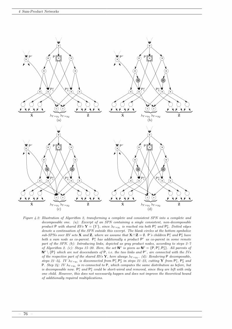
4 Sum-Product Networks
︸ ︷︷ ︸λY=y1
λY=y2
︸ ︷︷ ︸X
︸ ︷︷ ︸Z
P
Po1 Po2
Pr
(a)
︸ ︷︷ ︸λY=y1
λY=y2
︸ ︷︷ ︸X
︸ ︷︷ ︸Z
P
Po1 Po2
Pr
(b)
︸ ︷︷ ︸λY=y1
λY=y2
︸ ︷︷ ︸X
︸ ︷︷ ︸Z
P
Po1 Po2
Pr
(c)
︸ ︷︷ ︸λY=y1
λY=y2
︸ ︷︷ ︸X
︸ ︷︷ ︸Z
P
Po1 Po2
Pr
(d)
Figure 4.2: Illustration of Algorithm 2, transforming a complete and consistent SPN into a complete anddecomposable one. (a): Excerpt of an SPN containing a single consistent, non-decomposableproduct P with shared RVs Y = Y , since λY=y1 is reached via both Po1 and Po2. Dotted edgesdenote a continuation of the SPN outside this excerpt. The blank circles at the bottom symbolizesub-SPNs over RV sets X and Z, where we assume that X∩Z = ∅. P’s children Po1 and Po2 haveboth a sum node as co-parent. Po1 has additionally a product Pr as co-parent in some remotepart of the SPN. (b): Introducing links, depicted as gray product nodes, according to steps 2–7of Algorithm 2. (c): Steps 15–20. Here, the set No is given as No = P,Po1,Po2. All parents ofNo \ P which are not descendants of P, i.e. the two links and Pr, are connected with the IVsof the respective part of the shared RVs Y, here always λY=y1 . (d): Rendering P decomposable,steps 21–24. IV λY=y1 is disconnected from Po1,P
o2 in steps 21–23, cutting Y from Po1, Po2 and
P. Step 24: IV λY=y1 is re-connected to P, which computes the same distribution as before, butis decomposable now. Po1 and Po2 could be short-wired and removed, since they are left with onlyone child. However, this does not necessarily happen and does not improve the theoretical boundof additionally required multiplications.
– 76 –

4.4 Generalized Sum-Product Networks
P
︸ ︷︷ ︸λX=x1
λX=x2
︸ ︷︷ ︸λY=y1
λY=y2
(a)
P
︸ ︷︷ ︸λX=x1
λX=x2
︸ ︷︷ ︸λY=y1
λY=y2
(b)
P
︸ ︷︷ ︸λX=x1
λX=x2
︸ ︷︷ ︸λY=y1
λY=y2
(c)
Figure 4.3: Illustration of Algorithm 2, transforming a complete and consistent, but not decomposable SPTinto a complete and decomposable one. This demonstrates that using non-decomposable productsis wasteful in SPTs (cf. Proposition 4.3), since after performing Algorithm 2, the SPT computesthe same distribution, but requires fewer multiplications. (a): Complete and consistent SPTover two binary RVs X,Y , containing a non-decomposable product P. (b): Effect of steps 21–23of Algorithm 2, saving 3 multiplications. (c): Effect of steps 24 of Algorithm 2, reconnectingλX=x1 to P, re-introducing 1 multiplication.
4.4 Generalized Sum-Product Networks
So far, we considered SPNs defined as in [79], using IVs to represent the states of discrete RVs.In [40, 71], a recursive definition of SPNs was introduced, generalizing SPNs to continuous RVsand discrete RVs with infinitely many states. The basic insight is that IVs can be interpretedas discrete distribution assigning all probability mass to a single state [79]. To generalize SPNs,we replace IVs λX=x by distributions DY, where DY is either a PMF, a PDF or a mixeddistribution over any set of RVs Y, cf. Section 2.1. To these DY we refer as distribution nodes,input distributions or simply as distributions. We define generalized SPNs as follows:
Definition 4.15 (Generalized Sum-Product Network). A sum-product network S = (G,w) overRVs X is a rooted acyclic directed graph G = (V,E) and a set of nonnegative parameters w. Vcontains three types of nodes: distribution nodes, sum nodes and product nodes. All leaves of Gare distributions and all internal nodes are either sums or products, defined as follows:
1. Input distributions DY for some Y ⊆ X. The scope of DY is sc(DY) := Y.
2. Sums over nodes with identical scopes, i.e. sc(C′) = sc(C′′), ∀C′,C′′ ∈ ch(S):
S =∑
C∈ch(S)
wS,C C, (4.50)
where the weight wS,C ∈ w is associated with the edge (S → C) ∈ E. The scope of a sumnode is sc(S) =
⋃C∈ch(S) sc(C).
3. Products over nodes with non-overlapping scopes, i.e. sc(C′) ∩ sc(C′′) = ∅, ∀C′,C′′ ∈ch(P), C′ 6= C′′:
P =∏
C∈ch(P)
C. (4.51)
The scope of a product node is sc(P) =⋃
C∈ch(P) sc(C).
– 77 –

4 Sum-Product Networks
w is the set of all weights associated with sum nodes. The distribution computed by S is thedistribution computed by the root node.
In Definition 4.15 we already require that sums are complete and products are decomposable,see Definitions 4.9 and 4.11. Theorem 4.2 also clearly holds here, so without loss of generalitywe assume generalized SPNs to be locally normalized, cf. Section 4.3.3. Thus, in generalizedSPNs, each node readily represents a distribution over its scope:
• Leaves are distributions per definition.
• Products are distributions assuming independence of its child distributions.
• Sums are mixture distributions.
That is, generalized SPNs represent PMFs, PDFs or mixed distributions over X. Note that wedo allow heterogeneous scopes of the input distributions, i.e. when we have a DY with Y ∈ Y,we can have another DY′ with Y ∈ Y′ and Y 6= Y′. In the most extreme case, we can havedistributions DY for all possible nonempty subsets of Y ⊆ X, as long as completeness anddecomposability hold. However, we require that for discrete RVs X, every DY with X ∈ Yis a PMF with respect to X. Likewise, we require that for continuous RVs X, every DY withX ∈ Y is a PDF with respect to X. From now on, we refer to generalized SPNs simply as SPNs.To distinguish them from SPNs according to Definition 4.4, we denote the latter as finite-stateSPNs.
Although SPNs generalize finite-state SPNs by replacing IVs with general distributions, itwill be helpful in many cases to use IVs as input distributions for finite-state RVs. This allowsus to define an extended network polynomial and a corresponding differential approach:
Definition 4.16 (Extended network polynomial). Let p(X,Z) be a probability distribution overRVs X, Z, where Z have finitely many states. The extended network polynomial fep is definedas
fep (X,λ) =∑
z∈val(Z)
p(X, z)∏Z∈Z
λZ=z[Z]. (4.52)
Similar as the network polynomial in (4.13), the extended network polynomial allows us tomarginalize over any Z ∈ HZ and to apply the differential approach with respect to Z. To seethis, let us split X into disjoint Y and Y′, where for Y we have partial evidence Y , for Y′ wehave complete evidence y′, and evidence Z for Z, cf. Section 4.1. To evaluate this evidence forp(X,Z), we compute∑
z∈Z
∫Yp(y,y′, z) dy =
∫Yfep (y,y′,λ(Z)) dy, (4.53)
i.e. similar as the network polynomial, the extended network polynomial “takes care” aboutmarginalization over Z by simply setting the corresponding IVs. We can also apply the differ-ential approach, e.g.
∂∫Y f
ep (y,y′,λ(Z)) dy
∂λZ=z=
∑z′∈Z[Z\Z]
∫Yp(y,y′, z, z′) dy. (4.54)
Not surprising, when using exclusively IVs as input distributions for some set Z of finite-stateRVs, an SPN computes an extended network polynomial:
– 78 –

4.4 Generalized Sum-Product Networks
Proposition 4.4. Let X be a set of RVs and Z a set of finite-state RVs. An SPN S overX ∪ Z, where for all Z ∈ Z, z ∈ val(Z) the IVs λZ=z are used as input distributions. ThenS computes the extended network polynomial feS .
Proof. The proof works similar as for Proposition 4.2, showing by induction that every node in Scomputes the extended network polynomial over the distribution represented by this node.
We now aim to derive the same inference scenarios for SPNs as for finite-state SPNs. Inheritedfrom the theory on network polynomials and the differential approach, there are three inferencescenarios for complete and decomposable finite-state SPNs, which can be exactly solved withsimple upward and/or downward passes:
1. Evaluation of distribution S(x) for sample x ∈ val(X).
2. Partial marginalization, i.e. for Y ⊆ X, Y′ = X \Y, evaluation of∫YS(y,y′) dy, (4.55)
for partial evidence Y ∈ HY and complete evidence y′ ∈ val(Y′).
3. Evaluation of modified evidence/marginal posteriors for all X ∈ X simultaneously, i.e. forY ⊆ X, Y′ = X \Y, compute∫
Y[Y\X]S(X,y,y′[Y′ \ X]) dy ∝ S(X |Y [Y \ X],y′[Y′ \ X]), (4.56)
for Y ∈ HY, y′ ∈ val(Y′).
(1.): Evaluation of S(x) works exactly the same for generalized SPNs, by simply evaluatingall nodes from the leaves to the root, i.e. by one upwards pass. Note that inference scenario (2.)subsumes (1.).
(2.): Partial marginalization also works by a single upwards pass, since we can “pull” theintegrals in (4.55) over all sum and product nodes, down to the input distributions. To see this,consider an arbitrary sum S for which, due to completeness, (4.55) can be written as∫
YS(y,y′) dy =
∫Y
∑C∈ch(S)
wS,C C(y,y′) dy (4.57)
=∑
C∈ch(S)
wS,C
∫YC(y,y′) dy, (4.58)
i.e. the integrals of a sum node equals the weighted sum of the integrals of the child nodes.
Now consider an arbitrary product node P. Due to decomposability we are allowed to swapintegrals and the product, i.e. we have∫
YP(y,y′) dy =
∫Y
K∏k=1
Ck(y[sc(Ck)],y′[sc(Ck)]) dy (4.59)
=
K∏k=1
[∫Y[sc(Ck)]
Ck(yk,y′[sc(Ck)]) dy
k
](4.60)
We see that the integral of a product node equals the product of integrals of the child nodes,over their respective scopes. Furthermore, the same integrals are required for any co-parentsof the children of S or P. Therefore, we can perform integration (4.55) by performing the
– 79 –

4 Sum-Product Networks
corresponding integrations at the input distributions over their respective scopes, and evaluatingsum and product nodes in the usual way.
As a sanity check, let us see if this agrees with finite-state SPNs.
Example 4.1 (Finite-state RVs). Let X be a set of finite-state RVs and introduce for each X,x ∈ val(X) the input distributions
DX,x(x′) = 1(x = x′). (4.61)
To evaluate evidence Y, y′, we simply perform the marginalization at the input distributionsand evaluate sums and products the usual way. When X ∈ Y, and X = Y [X], this yields
∑x′∈X
DX,x(x′) =
1 if x ∈ X0 otherwise,
(4.62)
which reproduces the mapping for IVs (4.11). When X ∈ Y′, and y′[X] = x′ we get
DX,x(x′) =
1 if x = x′
0 otherwise(4.63)
which reproduces (4.9).
For finite-state RVs, we yield the same result for marginalization as dictated by the theory overnetwork polynomials. Now, let us consider continuous RVs, using single-dimensional Gaussiansas input distributions.
Example 4.2 (Continuous RVs, single-dimensional Gaussians). Assume X are continuous RVsand for each X ∈ X we have K Gaussian input distributions DX,1, . . . ,DX,K , all with theirindividual mean and standard deviation. Let Y ⊂ X and Y′ = X \Y. To evaluate the marginaldistribution of Y′ for some y′, we need to marginalize Y, i.e. for all Y ∈ Y, Y [Y ] = R. Foreach Y we get
∫Y[Y ] DY,k = 1 and each Gaussian DY ′,k is evaluated at y′[Y ′]. These values serve
as input to the SPN and are propagate though all sum and product nodes, yielding the desiredevaluation of the marginal distribution of Y′.
Now assume more generally that we have evidence that each Y ∈ Y takes a value in some“simple” set Y [Y ], say an interval, or the union of a few intervals. In this case we still caneasily compute
∫Y[Y ] DY,k ≤ 1 using the Gaussian CDF. Again evaluating DY ′,k for y′[Y ′], and
propagating these values through the SPN, we get∫y∈YS(y′,y) dy = S(y′ |y ∈ Y)PS(y ∈ Y), (4.64)
where PS denotes the probability measure defined by PDF S, cf. Section 2.1. In particular, whenY′ = ∅, the SPN evaluates PS(y ∈ Y).
These two examples used only distributions over single RVs. We want to stress again, thatthis is not necessary: as long as marginalizations according to 4.55 can computed at the inputdistributions, the overall marginalization results from normal evaluation of the sum and productnodes. We can also be agnostic how these input distributions are represented. They might berepresented as BNs, MNs, ACs [84], or again as SPNs. The latter suggests a recursive way toconstruct SPNs, a view which is followed in [40,71].
(3.): Simultaneous evaluation of modified evidence/marginal posteriors for all X can be tack-led using the differential approach in extended network polynomials. Let X be the scope ofthe SPN and DX be the set of input distributions which have X in their scope. We define anarbitrary but fixed ordering of DX = DX,1, . . . ,DX,|DX | and define [D]X = k if D is the kth
– 80 –

4.4 Generalized Sum-Product Networks
distribution in DX . For each X, we introduce a latent RV ZX with val(ZX) = 1, . . . , |DX |.We denote these RVs as distribution selectors (DS) and let Z = ZX |X ∈ X be the set of allDS. Now we replace each distribution node D in the SPN by
D→ D×∏
X∈sc(D)
λZX=[D]X , (4.65)
and denote the result as gated SPN. To the product introduced in (4.65) we refer as gate PX,[D]X .An example of constructing a gated SPN is shown in Figure 4.4.5 In the following proposition
D1 D2 D3 D4
(a)
︸ ︷︷ ︸λZX=1 λZX=2 λZX=3
︸ ︷︷ ︸λZY =1 λZY =2 λZY =3
D1 D2 D3 D4
(b)
Figure 4.4: Constructing a gated SPN by introducing distribution selectors. Here we assume that sc(D1) =X, sc(D2) = sc(D3) = X,Y and sc(D4) = Y , and that they are the only distributionswith X or Y in their scope. (a): Excerpt of an SPN showing the input distributions over X andY . (b): Same excerpt with introduced DSs λZX=1, λZX=2, λZX=3, λZY =1, λZY =2, λZY =3. Thesingle parents of D1, D2, D3, D4 are the gates PX,1, PX,2 = PY,1, PX,3 = PY,2, PY,3, respectively.
we note some properties about gated SPNs.
Proposition 4.5. Let S be an SPN and Sg be its gated SPN. Then
1. Sg is an SPN over X ∪ Z.
2. S(X) = Sg(X) =∑
z∈val(Z) Sg(X, z).
3. For any X ∈ X and k ∈ 1, . . . , |DX |, let XD = sc(DX,k) and XR = X \XD. It holdsthat
Sg(X, ZX = k,Z \ ZX) = DX,k(XD)Sg(XR, ZX = k,Z \ ZX), (4.66)
i.e.
XD ⊥⊥ XR ∪ Z \ ZX |ZX (4.67)
In particular
Sg(X, ZX = k) = DX,k(XD)Sg(XR, ZX = k), (4.68)
For a fixed X, we split the sets Y and Y′ from (4.56) according to the distribution DX,k:
Yk = Y ∩ sc(DX,k), Y′k = Y′ ∩ sc(DX,k)
Yk = Y \ sc(DX,k), Y′k = Y′ \ sc(DX,k)(4.69)
5 For representing distribution nodes, we use symbol .
– 81 –

4 Sum-Product Networks
Then, using Proposition 4.5, we get
∫YS(y,y′) dy =
|DX |∑k=1
∫YSg(y,y′, ZX = k) dy (4.70)
=
|DX |∑k=1
(∫Y[Yk]
DX,k(yk,y′[Y′k]) dyk
) (∫Y[Yk]
Sg(yk,y′[Y′k], ZX = k) dyk
)︸ ︷︷ ︸
gX,k
(4.71)
To find the factors gX,k, note that the kth term in (4.70) can also be computed by the differentialapproach, setting all λZX=k = 1 and computing∫
YSg(y,y′, ZX = k) dy =
∂∫Y S
g(y,y′) dy
∂λZX=k. (4.72)
This derivative is given according to (4.42) and (4.46) as
∂∫Y S
g(y,y′) dy
∂λZX=k=∂∫Y S
g(y,y′) dy
∂PX,k
∫Y[Yk]
DX,k(yk,y′[Y′k]) dyk (4.73)
Comparing (4.71) and (4.73), we find that
gX,k =∂∫Y S
g(y,y′) dy
∂PX,k=∂∫Y S(y,y′) dy
∂DX,k(4.74)
The right hand side in (4.74) holds since all λZX=k = 1 and the structure above all DX,k in Sand above all PX,k in Sg is identical. Since for all k, X is contained either in Yk or in Yk, wefind the distribution over X with modified evidence by∫
Y[Y\X]S(X,y,y′[Y′ \ X]) dy = (4.75)
|DX |∑k=1
∫Y[Yk\X]
DX,k(X,yk,y′[Y′k \ X]) dyk∂∫Y S(y,y′) dy
∂DX,k, (4.76)
i.e. we input evidence as in inference scenario (2.), and find the derivatives ∂S∂DX,k
at each inputdistribution using backpropagation. These derivatives are used as weights of a linear combina-tion of distributions DX , evaluated anew for evidence in sc(DX,k) \ X. Similar as inferencescenario (2.), inference scenario (3.) reduces to the corresponding inference scenario at the in-put distributions. Note, that although we used gated SPNs and extended network polynomialsfor deriving this result, all required terms can be computed in the original SPN S. However,introducing the DS, which are artificially latent RVs, helped us in our approach. In the nextchapter, we go one step further and introduce a latent RV for each sum node in the SPN.
– 82 –

Foundations of Sum-Product Networks for Probabilistic Modeling
5Sum-Product Networks as Latent Variable
Models
In [79] a latent RV interpretation for SPNs was introduced, associating a latent RV with eachsum node, where each child of the sum corresponds to a state of the RV. In that way, the sumoperation can be interpreted as marginalization of this latent RV. This technique is often appliedto mixture distributions, as illustrated in the following example.
Example 5.1. Consider a mixture of Gaussians over RV X, whose PDF p is defined as:
p(X) =K∑k=1
wkN (X |µk, σk), (5.1)
where K is the number of components, µk and σk are the mean and the standard deviation ofthe kth component, and wk are the mixture weights, satisfying
wk ≥ 0,∑k
wk = 1. (5.2)
Eq. (5.1) has two interpretations:
1. It is a convex combination of K PDFs N (· |µk, σk) and thus a PDF.
2. It is the marginal distribution of a joint distribution over X,Z, defined as
p(X,Z) = p(Z) p(X |Z), (5.3)
where |val(Z)| = K, p(Z = zk) = wk and p(X |Z = zk) = N (X |µk, σk).
The second interpretation in this example has several advantages, e.g. that the EM algo-rithm can be applied for ML learning. In this chapter, we investigate in detail the latent RVinterpretation of sum nodes in SPNs.
5.1 Augmentation of SPNs
In [79], it was proposed to make the latent RVs explicit as depicted in Figure 5.1. For each sum
– 83 –

5 Sum-Product Networks as Latent Variable Models
S
(a)
S , Z
︸ ︷︷ ︸λZ=1 λZ=2 λZ=3
(b)
Figure 5.1: Augmenting SPN structure to explicitly introduce IVs representing states of a latent RV associ-ated with sum node S. (a): Part of an SPN containing a sum node S with three children. (b):Augmented structure explicitly containing IVs for each sum child.
node S, one introduces a latent RV Z whose states correspond with the children of S. The SPNstructure is augmented by introducing one product and one IV for each child, such that the sub-SPN rooted at this child is turned on/off by setting/unsetting its corresponding IV, as shown inFigure 5.1 (b). When all IVs are set to 1 the sum node S in Figure 5.1 (b) computes the samevalue as in Figure 5.1 (a). Since setting all IVs of Z to 1 corresponds to marginalizing Z, eachsum node can be interpreted as a latent, marginalized RV. Furthermore, the weights associatedto S should be interpretable as CPT of Z, conditioned on a certain context represented by theancestor sum nodes of S.
However, taking a closer look, we recognize that augmenting the SPN in this way is toosimplistic. Consider the augmentation of the SPN structure from Figure 5.1(a) within a largerstructural context, shown in Figure 5.2(a). Explicitly introducing the IVs corresponding to Zin Figure 5.2 (b) renders node S′ incomplete, since S is no descendant of N and therefore Z isnot in the scope of N. Since we require completeness of the SPN in order that setting all IVs ofZ corresponds the marginalization, this approach for augmenting the SPN is flawed.
Furthermore, note that S′ also corresponds to a latent RV Z ′. Although we know the proba-bility distribution of Z if Z ′ is in the state corresponding to P, namely the weights associatedto S, we do not know this distribution when Z ′ is in the state corresponding to N. Intuitively,we recognize that the state of Z is “irrelevant” when Z ′ is in the state corresponding to N,since it does not influence the resulting distribution over the model RVs X. Nevertheless, theprobabilistic model is not completely specified, which is unsatisfying.
A remedy for these problems is shown in Figure 5.2 (c), by augmenting the SPN structurefurther. We introduce the twin sum node S of S whose children are the IVs corresponding to Z.The twin S is connected as child of an additional product node which is interconnected betweenS′ and N. Since this new product node has scope sc(N) ∪ Z, S′ is rendered complete now. IfZ ′ takes the state corresponding to N (or actually the state corresponding to the new productnode), we now have a specified conditional distribution of Z, namely the weights of the twin sumnode S. Furthermore, given that all IVs of Z are set to 1, the network depicted in Figure 5.2 (c)still computes the same function as the network in Figure 5.2 (a), since S constantly outputs 1.
The question raises, which weights should be used for the twin sum node S. Basically, wecan assume arbitrary normalized weights, which will cause S to constantly output 1. Followingan esthetic and maximum entropy argument, however, we would assume uniform weights for S.While the choice of weights is not crucial for evaluating evidence in the SPN, it will however
– 84 –

5.1 Augmentation of SPNs
S
S′
P N
(a)
S , Z
S′
P N
︸ ︷︷ ︸λZ=1 λZ=2 λZ=3
(b)
S , ZS
S′
P N
︸ ︷︷ ︸λZ=1 λZ=2 λZ=3
(c)
Figure 5.2: Problems occurring when IVs of latent variables are introduced. (a): Larger part of the SPNdepicted in Figure 5.1 (a). In this example we assume that S /∈ desc(N). (b): Introducing IVsfor Z renders S′ incomplete. (c): Remedy by extending SPN structure further, introducing twinsum node S.
play a role when we discuss MPE inference in Section 5.3. For now, let us formally introducethe latent RV interpretation of sum nodes.
Definition 5.1 (Associated Latent RVs). Let S be an SPN over X. For each S ∈ S(S) weassume an arbitrary but fixed ordering of its children ch(S) = C1
S, . . . ,CKSS , where KS =
|ch(S)|. Let ZS be an RV on the same probability space as X, with val(ZS) = 1, . . . ,KS,6
6 For ease of discussion, we use the first KS integers as states of ZS.
– 85 –

5 Sum-Product Networks as Latent Variable Models
where state k corresponds to child CkS. We call ZS the latent RV associated with S. For sets ofsum nodes S we define ZS = ZS | S ∈ S.
To distinguish X from the latent RVs we will refer to the former as model RVs. Definition 5.1postulates latent RVs associated with sum nodes, defined on the same probability space as X,and where each state corresponds to a sum child. We will complete this definition by specifyingthe augmented SPN, defining the joint distribution of X and the associated RVs. First we needsome more definitions.
Definition 5.2 (Sum Ancestors/Descendants). Let S be an SPN and N a node in S. We definesum ancestors/descendants as
ancS(N) := anc(N) ∩ S(S) (5.4)
descS(N) := desc(N) ∩ S(S) (5.5)
Definition 5.3 (Conditioning sums). Let S be an SPN over X. For each sum node S we definethe conditioning sums of S as
Sc(S) := Sc ∈ ancS(S) \ S | ∃C ∈ ch(Sc) : S /∈ desc(C). (5.6)
Definition 5.4 (Twin weights). Let S be an SPN over X. Let w be a set of nonnegative weightscontaining a weight wS,C for each wS,C, where wS,C ≥ 0,
∑C∈ch(S) wS,C = 1. We call w a set of
twin weights and wS,C is the twin weight of wS,C.
We now define augmented SPNs, explicitly introducing the associated RVs in the SPN andspecifying the completed probabilistic model.
Definition 5.5 (Augmentation of SPN). Let S be an SPN over X, w be a set of twin weightsand S ′ be the result of Algorithm 3. S ′ is called the augmented SPN, denoted as S ′ =: aug(S).Within the context of S ′, is CkS is called the kth former child of S. The introduced product nodePkS is called link of S, CkS and λZS=k, respectively. The sum node S, if introduced, is called thetwin sum node of S.
In the first part of Algorithm 3 (1–8) we introduce the links PkS which are interconnectedbetween the sum node S and its kth child. Each link PkS has a single parent, namely S, andsimply copies the former child CkS, which might have more than one parent. Note that wealready used links in Algorithm 2 for the proof for Theorem 4.3. In steps 10–12, we introduceIVs corresponding to the associated RV ZS, which is the augmentation according to [79]. Asillustrated in Figure 5.2, this can render other sum nodes incomplete. Thus, when necessary,we introduce a twin sum node in steps 14–20, to treat this problem. Note that we assume a fullset of twin weights, even when for some sum nodes no twin node is introduced. This will easediscussion in Section 5.2. The following proposition states the soundness of augmentation.
Proposition 5.1. Let S be an SPN over X, S ′ = aug(S) and Z := ZS(S). Then S ′ is acomplete and decomposable SPN over X ∪ Z with S ′(X) ≡ S(X).
Proposition 5.1 states that the augmented SPN represents the same distribution over X asthe original SPN when the latent RVs Z are marginalized, while being a completely specifiedprobabilistic model over X and Z. Clearly, the augmented SPN will usually not be generated forpractical purposes, but we will mainly consider it as a theoretical tool. The following exampleillustrates the process of augmentation.
– 86 –

5.1 Augmentation of SPNs
Algorithm 3 Augment SPN S∀S ∈ S(S), ∀k ∈ 1, . . . ,KS let wS,k = wS,CkS
, wS,k = wS,CkS
Introduce links:1: for S ∈ S(S) do2: for k = 1 . . .KS do3: Introduce a new product node PkS in S4: Disconnect CkS from S5: Connect CkS as child of PkS6: Connect PkS as child of S with weight wS,k
7: end for8: end for
Introduce IVs and twins:9: for S ∈ S(S) do
10: for k ∈ 1, . . . ,KS do11: Connect new IV λZS=k as child of PkS12: end for13: if Sc(S) 6= ∅ then14: Introduce a twin sum node S in S15: ∀k ∈ 1, . . . ,KS: connect λZS=k as child of S, and let wS,λZS=k
= wS,k
16: for Sc ∈ Sc(S) do17: for k ∈ k | S 6∈ desc(PkSc) do18: Connect S as child of PkSc19: end for20: end for21: end if22: end for
Example 5.2 (Augmentation of SPN). Figure 5.3(a) shows an example SPN over three RVsX1, X2, X3. Figure 5.3(b) shows the corresponding augmented SPN.
It should be noted that augmentation presented here is not necessarily the only way to in-troduce latent RVs, and, that sum nodes have sometimes a more natural interpretation. Forsome examples see Section 6.1, where sum nodes, or more precisely sum-weights, have a naturalinterpretation of CPTs of model RVs. However, due to Proposition 5.1 we have neverthelessalways the option to perform augmentation and interpret sum nodes as latent RVs. We couldalso construct augmented SPNs of augmented SPNs, i.e. consider aug(aug(S)), since aug(S)is simply a complete and decomposable SPN over X, Z. This would blow up the RV set furtherand introduce redundant copies of the latent RVs introduced in the first augmentation.
– 87 –

5 Sum-Product Networks as Latent Variable Models
S1
S2 S3
S4
︸ ︷︷ ︸X1
︸ ︷︷ ︸X2
︸ ︷︷ ︸X3
(a)
S1
S2 S3
S4
︸ ︷︷ ︸X1
︸ ︷︷ ︸X2
︸ ︷︷ ︸X3
S2 S3
S4
︸ ︷︷ ︸λZ
S1=1...3
︸ ︷︷ ︸λZ
S2=1...3
︸ ︷︷ ︸λZ
S3=1...3
︸ ︷︷ ︸λZ
S4=1...2
(b)
Figure 5.3: Augmentation of an SPN. (a): Example SPN over X = X1, X2, X3, containing sum nodes S1,S2, S3 and S4. (b): Augmented SPN, containing IVs corresponding to ZS1 , ZS2 , ZS3 , ZS4 , linksand twin sum nodes S2, S3, S4. For nodes introduced by augmentation smaller circles are used.
5.2 Independencies and Interpretation of Sum Weights
We now investigate certain conditional independencies which hold in the augmented SPN, allow-ing us to interpret the augmented SPN as BN. Furthermore, we also formalize the interpretationof sum weights as CPTs in the corresponding BN. To this end, we introduce the notion of con-figured SPNs.
Definition 5.6 (Configured SPN). Let S be an SPN over X, and let Y ⊆ ZS(S) and y ∈ val(Y).The configured SPN Sy is obtained by Algorithm 4.
Algorithm 4 Configure SPN
1: Sy ← aug(S)2: for Y ∈ Y do3: for y ∈ val(Y ), y 6= y[Y ] do4: Delete λY=y and its corresponding link5: end for6: end for7: Delete all nodes in Sy which are not reachable from the root
Example 5.3 (Configured SPN). Two examples of configured SPNs of the SPN in Example 5.2,using two different y, are shown in Figure 5.4.
Intuitively, the configured SPN isolates the computational structure selected by y. All sumedges which “survive” Algorithm 4 are equipped with the same weights as in the augmentedSPN. Therefore, a configured SPN is in general not locally normalized. We note the followingproperties of configured SPNs.
Proposition 5.2. Let S be an SPN over X, Y ⊆ ZS(S) and Z = ZS(S) \Y. Let y ∈ val(Y)and let S ′ = aug(S). It holds that
– 88 –

5.2 Independencies and Interpretation of Sum Weights
S1
S2 S3
S4
︸ ︷︷ ︸X1
︸ ︷︷ ︸X2
︸ ︷︷ ︸X3
S2 S3
S4
λZS1=1
λZS2=2
︸ ︷︷ ︸λZ
S3=1...3
︸ ︷︷ ︸λZ
S4=1...2
(a)
S1
S2
S4
︸︷︷︸X1
︸︷︷︸X2
︸ ︷︷ ︸X3
S3
λZS1=1
λZS2=2
︸ ︷︷ ︸λZ
S3=1...3
︸ ︷︷ ︸λZ
S4=1...2
(b)
S1
S2 S3
S4
︸ ︷︷ ︸X1
︸ ︷︷ ︸X2
︸ ︷︷ ︸X3
S2 S3
S4
︸ ︷︷ ︸λZ
S1=1...3
λZS2=3 λZ
S3=1
︸ ︷︷ ︸λZ
S4=1...2
(c)
S1
S2 S3
S4
︸ ︷︷ ︸X1
︸︷︷︸X2
︸ ︷︷ ︸X3
S2 S3
S4
︸ ︷︷ ︸λZ
S1=1...3
λZS2=3 λZ
S3=1
︸ ︷︷ ︸λZ
S4=1...2
(d)
Figure 5.4: Configured SPNs of SPN shown in Figure 5.3. (a): Augmented SPN before performing step 7of Algorithm 4 for Y = ZS1 , ZS2 and configuration y = (1, 2). (b): Configured SPN resultingfrom removing unreachable nodes from (a). (c), (d): Similar to (a), (b), for for Y = ZS2 , ZS3and configuration y = (3, 1).
1. Each node in Sy has the same scope as its corresponding node in S ′.
2. Sy is a complete and decomposable SPN over X ∪Y ∪ Z.
3. For any node N in Sy with sc(N) ∩Y = ∅, we have that SyN = S ′N.
4. For y′ ∈ val(Y) it holds that
Sy(X,Z,y′) =
S ′(X,Z,y′) if y′ = y
0 otherwise(5.7)
The following theorem shows certain conditional independencies which hold in the augmented
– 89 –

5 Sum-Product Networks as Latent Variable Models
SPN. For the proof, we need the following lemma.
Lemma 5.1. Let S be an SPN over X, let S be a sum node in S and Z = ZancS(S)\S. Forany z ∈ val(Z), the configured SPN Sz contains either S or its twin S, but not both.
Theorem 5.1. Let S be an SPN over X, S be an arbitrary sum in S and wk = wS,CkS, wk = wS,CkS
,
k = 1, . . . , |ch(S)|. Let
Z := ZS, (5.8)
Z := ZancS(S) \ Z, (5.9)
Yd := sc(S) ∪ ZdescS(S) \ Z, (5.10)
Yn := (X ∪ ZS(S)) \ (Yd ∪ Z ∪ Z). (5.11)
Furthermore, let S ′ = aug(S). There exists a two-partition of val(Z), i.e. Z, Z: Z ∪ Z =val(Z), Z ∩ Z = ∅,7 such that
∀z ∈ Z : S ′(Z = k,Yn, z) = wk S ′(Yn, z), and (5.12)
∀z ∈ Z : S ′(Z = k,Yn, z) = wk S ′(Yn, z). (5.13)
Proof.By Lemma 5.1, for each z ∈ val(Z) the configured SPN Sz contains either S or S, but not
both. Let Z be the subset of val(Z) such that S is in Sz and Z be the subset of val(Z) suchthat S is in Sz.
Fix Z = k and z ∈ Z. We want to compute S ′(Z = k,Yn, z), i.e. we marginalize Yd.According to Proposition 5.2 (4.), this equals Sz(Z = k,Yn, z). According to Proposition 5.2(3.), the sub-SPN rooted at former child CkS is the same in S ′ and Sz. Since S ′ is locallynormalized, this sub-SPNs is also locally normalized in Sz. Since the scope of the former childCkS is a sub-set of Yd and λZ=k = 1, the link PkS outputs 1. Since λZ=k′ = 0 for k′ 6= k, the sumS outputs wk.
Now consider the set of nodes in Sz which have Z in their scope, not including λZ=k and PkS.Clearly, since S is not in Sz, this set must be anc(S). Let N1, . . . ,NL be a topologically orderedlist of anc(S), where S is N1 and NL is the root. Let Yn
l := sc(Nl) ∩Yn and Zl := sc(Nl) ∩ Z.We show by induction that for l = 1, . . . , L, we have
Nl(Z = k,Ynl , z[Zl]) = wk Nl(Y
nl , z[Zl]). (5.14)
Since Yn1 = ∅ and Z1 = ∅, and N1(Z = k) = wk, the induction basis holds. Assume that (5.14)
holds for all N1, . . . ,Nl−1. If Nl is a sum, we have due to completeness
Nl(Z = k,Ynl , z[Zl]) =
∑C∈ch(Nl)
wNl,C C(Z = k,Ynl , z[Zl]) (5.15)
=∑
C∈ch(Nl)
wNl,Cwk C(Ynl , z[Zl]) (5.16)
= wk Nl(Ynl , z[Zl]), (5.17)
i.e. the induction step holds for sums. When Nl is a product, due to decomposability, it must
7 Here, Z and Z are not necessarily elements from HZ.
– 90 –

5.2 Independencies and Interpretation of Sum Weights
have a single child C′ with Z ∈ sc(C′). We have
Nl(Z = k,Ynl , z[Zl]) = C′(Z = k, sc(C′) ∩Yn
l , z[sc(C′) ∩ Z])∏
C∈ch(Nl)\C′
C(·) (5.18)
= wk C′(sc(C′) ∩Yn, z[sc(C′) ∩ Z])
∏C∈ch(Nl)\C′
C(·) (5.19)
= wk Nl(Ynl , z[Zl]), (5.20)
i.e. the induction step holds for products. Therefore, by induction, (5.14) also holds for the root,and (5.12) follows.
Now fix the input to arbitrary Z = k and z ∈ Z. Clearly, S outputs wk and (5.13) can beshown in similar way as (5.12).
Corollary 5.1. Make the same assumptions as in Theorem 5.1. In S ′, we have
Z ⊥⊥ Yn |Z. (5.21)
Furthermore we have
S ′(Z = k |yn, z) = S ′(Z = k | z) =
wk if z ∈ Zwk if z ∈ Z
(5.22)
Theorem 5.1 and Corollary 5.1 show that the weights and twin weights of a sum node S canbe interpreted as a conditional probability table (CPT) of the associated RV ZS. More precisely,given that the sum node ancestors “select a path” to S, i.e. z ∈ Z, then wS,CkS
is the probability
that ZS is in its kth state. Given the complementary event z ∈ Z, the corresponding twin weightwS,CkS
is the corresponding conditional probability.
We now also see an independency structure in augmented SPNs: a latent RV correspondingto S is conditional independent of all model RVs which are not in the scope of S, when the RVscorresponding to its sum ancestors are observed. It is also independent from all other latentRVs corresponding to sum nodes which are neither ancestors nor descendants of S. This is thecorrespondent to the local conditional independence statements BNs, cf. Theorem 3.1:
An RV is independent from its non-descendants, given its parents.
Given an SPN S, we can now construct an IMAP of aug(S) expressed via a BN. In the IMAP,we connect ZS as child of all ZancS(S) \ ZS and connect all model RVs which are in the scopeof S as child of ZS. As an example, Figure 5.5 (a) shows the augmented SPN from Figure 5.3and Figure 5.5 (b) its corresponding IMAP.
Furthermore, when all input distributions of the SPN are over single RVs, we can concludethat all model RVs are independent given all the latent RVs. In this case, we can interpretthe augmented SPN as a naive Bayes mixture model with a structured latent RV ZS(S), whosestate-space grows exponentially in the number of sum nodes in the SPN. This is illustratedin Figure 5.5 (c). In the naive Bayes interpretation, the input distributions take the role ofconditional distributions over the model RVs, which are shared among the exponentially manylatent states of ZS(S).
The IMAP representation shows that an SPN can be interpreted as hierarchical mixture model.However, the representation of an SPN as BN obscures the highly constrained structure of theCPTs of the augmented SPN. Consider an arbitrary sum node S and let Za = ZancS(S)\S insome SPN. In general, the associated RV ZS can depend on the state of all RVs Za. Thus,in a general BN the CPT for ZS would require |val(Za)| (|val(ZS)| − 1) parameters. Thisparameterization grows exponentially in |Za|.
– 91 –

5 Sum-Product Networks as Latent Variable Models
S1
S2 S3
S4
︸ ︷︷ ︸X1
︸ ︷︷ ︸X2
︸ ︷︷ ︸X3
S2 S3
S4
︸ ︷︷ ︸ZS1
︸ ︷︷ ︸ZS2
︸ ︷︷ ︸ZS3
︸ ︷︷ ︸ZS4
(a)
ZS1
ZS2 ZS3 ZS4
X1 X2 X3
(b)
ZS(S)
X1 X2 X3
(c)
Figure 5.5: Dependency structure of an augmented SPN. (a): Augmented SPN from Figure 5.3. (b): Cor-responding IMAP represented as BN. (c): Naive Bayes interpretation of augmented SPN.
However, the state space of Za is two-partitioned into Z and Z. For all states in Z, theconditional distribution of ZS is constant and given by the weights of S, and for Z the conditionaldistribution is given by the twin weights, which are the same as the weights of the twin sumnode S, if it exists. Thus, the CPT of ZS is highly constrained and can be represented by2 (|val(ZS)|−1) parameters in the augmented SPN. Furthermore, the twin weights will typicallybe set to the uniform distribution, so that we actually have |val(ZS)|−1 free parameters for ZS,i.e. the original SPN parameters.
The two-partition of val(Za) can be made explicit by further introducing a binary RV YSwith val(YS) = yS, yS where YS = yS ⇔ Za ∈ Z and YS = yS ⇔ Za ∈ Z. YS can be seen asswitching parent of ZS which, when observed, renders ZS independent from Za. This switchingparent can also be explicitly introduced in the augmented SPN as depicted in Figure 5.6. Herewe simply introduce two new IVs λYS=yS and λYS=yS , which switch on/off the output of S andS, respectively. It is easy to see that when these IV are constantly set to 1, i.e. when YS ismarginalized, the augmented SPN performs exactly the same computations as before. It isfurthermore easy to show that completeness and decomposability of the augmented SPN aremaintained when the switching parent is introduced. Introducing the switching parent allowsto derive the EM algorithm for SPN-weights, cf. Section 6.3.
– 92 –

5.3 Most Probable Explanation and Maximum A-posterior Hypothesis
SS
︸ ︷︷ ︸λZS=1 λZS=2 λZS=3
(a)
SS
︸ ︷︷ ︸λZS=1 λZS=2 λZS=3
λYS=ySλYS=yS
P
(b)
Figure 5.6: Explicitly introducing a switching parent YS in an augmented SPN. (a): Part of an augmentedSPN containing a sum node with three children and its twin. (b): Explicitly introduced switchingparent YS using IVs λYS=yS and λYS=yS
.
5.3 Most Probable Explanation and Maximum A-posteriorHypothesis
As discussed in Section 4.4, SPNs allow to perform several inference scenarios efficiently, likeevaluating the SPN distribution for complete evidence, partial marginalization and computingthe marginal posteriors given some evidence. In [79], SPNs were applied for reconstructing datausing MPE inference. Given some distribution p over X and partial evidence X ∈ HX, X 6= ∅,MPE can be formalized as finding
x∗ = arg maxx∈X
p(x). (5.23)
We assume here that p has a maximum in X , which, unless X is closed, does not necessarily existin the case of continuous RVs. MPE inference according to (5.23) generalizes MPE inference asdefined in Section 3.4, i.e. finding
arg maxxq∈val(Xq)
p(xq,xo). (5.24)
This scenario is a special case of (5.23), where ∀X ∈ Xq : X [X] = val(X) and ∀X ∈ Xo : X [X] =xo[X]. MPE defined as in (5.23) allows more generally to incorporate constraints on thedomain of the RVs, as illustrated in the following example.
Example 5.4. Let p be a distribution over X1, X2, X3 and we have evidence that X1 = x1 andthat X2 ≤ 42. Using X = x1 × [−∞, 42] × R and solving (5.23), we find the most probablesolution x∗ consistent with our evidence.
MPE is a special case of MAP, defined as finding
arg maxy∈Y
∫Zp(y, z) dz, (5.25)
for some two-partition of X, i.e. X = Y∪Z. Similar as for MPE, this generalizes MAP inferenceas defined in Section 3.4. MAP reduces to MPE when Y = X. Both MPE and MAP are NP-hardin general BNs [8, 54, 68, 69], and MAP is inherently harder than MPE [54, 69]. Theoretically,
– 93 –

5 Sum-Product Networks as Latent Variable Models
this is reflected that the decision versions of MPE is NP-complete, while the decision versionof MAP is NPPP-complete [54, 69]. In practice this means that in model classes which allow tosolve MPE efficiently, the MAP problem typically remains hard to solve.
In [79] it is stated that the MPE solution can be found efficiently in SPNs, where maximizationis over the model RVs X and the latent RVs Z represented by the sum nodes. For this purpose,a Viterbi-style algorithm is used: each sum node is replaced by a max node, i.e. a node whichoutputs the maximum of its child nodes. To find the MPE solution, back-tracking from theroot to the leave nodes is performed, where each sum node selects a maximizing child andeach product nodes selects all of its children. However, as discussed at the beginning of thischapter, the latent RV interpretation in [79] is incomplete, since the latent RV model in [79]does not specify the distribution of “irrelevant” latent RVs. We proposed the augmented SPNas a remedy for this issue. In this section we show that the algorithm proposed in [79] indeedfinds an MPE solution when applied to the augmented SPN. However, applying this algorithmto the non-augmented SPN corresponds to an unfortunate implicit parameter selection for thetwin sum nodes and leads to a phenomenon we call low-depth bias.
5.3.1 MPE Inference in Augmented SPNs
We formally investigate MPE using max-product networks.
Definition 5.7 (Max-Product Network). Let S be an SPN over X. The max-product network(MPN) S of S is a network obtained as follows:
• Replace each distribution node D by a maximizing distribution node D : Hsc(D) 7→ [0,∞],defined as
D(Y) := maxy∈Y
D(y) (5.26)
• Replace each sum node S in S by a max node S. The outgoing edges of a max node areequipped with the same weights as for its corresponding sum node. A max node is definedas
S := maxC∈ch(S)
wS,C C. (5.27)
• Each product P in S corresponds to a product P in S.
The scope in MPNs is defined as in SPNs.
The following theorem shows that for augmented SPNs the MPN computes the MPE proba-bility.
Theorem 5.2. Let S be an augmented SPN over X, where X already comprises the model RVsof the original SPN and the latent RVs introduced by augmentation, and let S the correspondingMPN. Let N be some node in S and N its corresponding node in S. For every X ∈ Hsc(N) wehave
N(X ) = maxx∈X
N(x). (5.28)
Proof. We proof the theorem using an inductive argument. The theorem clearly holds for anyD by definition. Consider a product P and assume the theorem holds for all ch(P). Then the
– 94 –
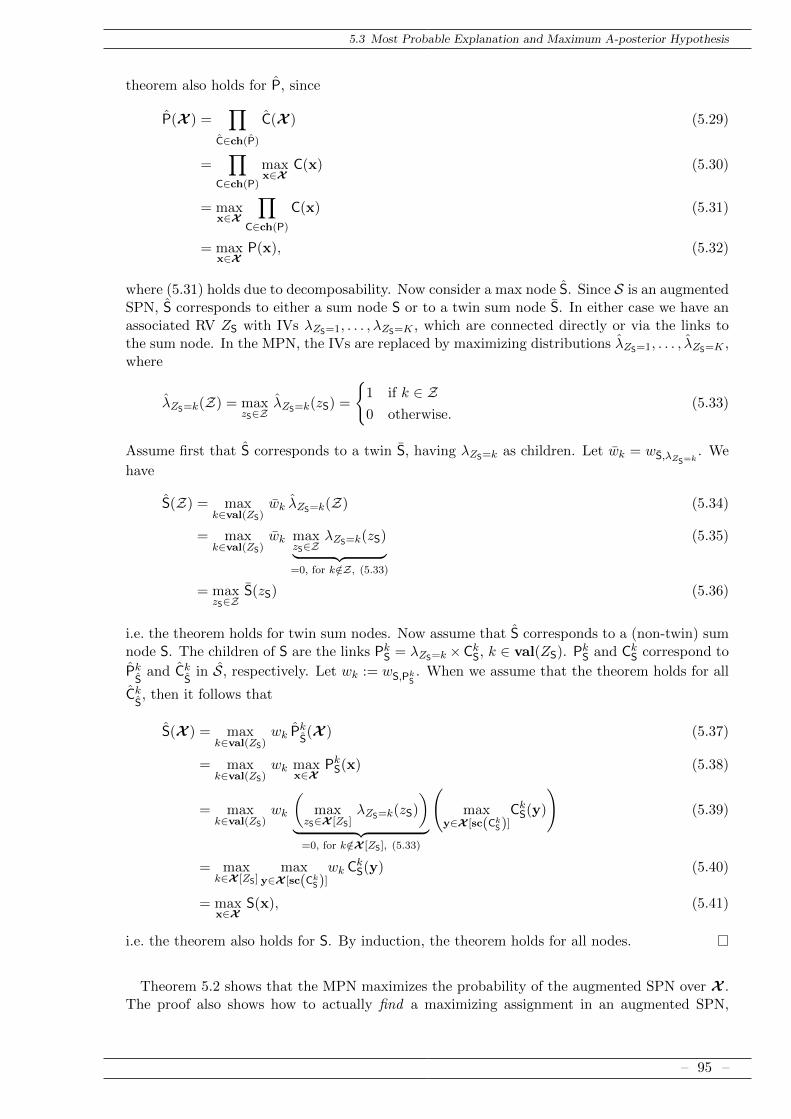
5.3 Most Probable Explanation and Maximum A-posterior Hypothesis
theorem also holds for P, since
P(X ) =∏
C∈ch(P)
C(X ) (5.29)
=∏
C∈ch(P)
maxx∈X
C(x) (5.30)
= maxx∈X
∏C∈ch(P)
C(x) (5.31)
= maxx∈X
P(x), (5.32)
where (5.31) holds due to decomposability. Now consider a max node S. Since S is an augmentedSPN, S corresponds to either a sum node S or to a twin sum node S. In either case we have anassociated RV ZS with IVs λZS=1, . . . , λZS=K , which are connected directly or via the links tothe sum node. In the MPN, the IVs are replaced by maximizing distributions λZS=1, . . . , λZS=K ,where
λZS=k(Z) = maxzS∈Z
λZS=k(zS) =
1 if k ∈ Z0 otherwise.
(5.33)
Assume first that S corresponds to a twin S, having λZS=k as children. Let wk = wS,λZS=k. We
have
S(Z) = maxk∈val(ZS)
wk λZS=k(Z) (5.34)
= maxk∈val(ZS)
wk maxzS∈Z
λZS=k(zS)︸ ︷︷ ︸=0, for k/∈Z, (5.33)
(5.35)
= maxzS∈Z
S(zS) (5.36)
i.e. the theorem holds for twin sum nodes. Now assume that S corresponds to a (non-twin) sumnode S. The children of S are the links PkS = λZS=k ×CkS, k ∈ val(ZS). PkS and CkS correspond to
PkS
and CkS
in S, respectively. Let wk := wS,PkS. When we assume that the theorem holds for all
CkS, then it follows that
S(X ) = maxk∈val(ZS)
wk PkS(X ) (5.37)
= maxk∈val(ZS)
wk maxx∈X
PkS(x) (5.38)
= maxk∈val(ZS)
wk
(max
zS∈X [ZS]λZS=k(zS)
)︸ ︷︷ ︸
=0, for k/∈X [ZS], (5.33)
(max
y∈X [sc(CkS)]CkS(y)
)(5.39)
= maxk∈X [ZS]
maxy∈X [sc(CkS)]
wk CkS(y) (5.40)
= maxx∈X
S(x), (5.41)
i.e. the theorem also holds for S. By induction, the theorem holds for all nodes.
Theorem 5.2 shows that the MPN maximizes the probability of the augmented SPN over X .The proof also shows how to actually find a maximizing assignment in an augmented SPN,
– 95 –

5 Sum-Product Networks as Latent Variable Models
Algorithm 5 MPE inference in augmented SPNs
1: For all sums S, let ch′(S) := CkS | k ∈ X [ZS]2: Evaluate X in corresponding MPN S (upwards pass)3: Initialize Q as empty queue4: Q ^ root node5: while Q not empty do6: N ^ Q7: if N is a sum node then8: Q ^ arg max
C∈ch′(N)
wN,C C(X [sc(C)])
9: else if N is a product node then
10: ∀C ∈ ch(N) : Q ^ C11: else if N is a distribution node then12: x∗[sc(N)] = arg max
x∈X [sc(N)]N(x)
13: end if14: end while15: return x∗
i.e. how to solve the MPE problem: In (5.30) we see that a product node is maximized byindependently maximizing each of its children. Therefore, finding a maximizing assignment forthe product is reduced to independently finding maximizing assignments for its children. In(5.35) and (5.38), we see that a (twin) sum node is maximized by maximizing the weightedmaxima of its children. Therefore, finding a maximizing assignment for a (twin) sum node isreduced to find a child with maximal weighted output and find a maximizing assignment for thischild. Algorithm 5 finds a maximizing state of the augmented SPN using back-tracking. In thisimplementation we use a queue Q, where Q ^ N and N ^ Q denote the enqueue and dequeueoperations, respectively. This is the same algorithm as proposed in [79], which was, however,applied to general SPNs, i.e. SPNs which are not augmented SPNs. Does this still correspondto an MPE solution? The answer is yes, but we implicitly use deterministic (zero-one) weightsfor the twin sum nodes.
To show this, let us modify Algorithm 5, such that it can be applied to an arbitrary (notaugmented) SPN, but returning the MPE solution of the corresponding augmented SPN. Suchan algorithm is also required for practical applications, since we usually do not want to explicitlygenerate the augmented SPN. Algorithm 6 is such a modification of Algorithm 5, simulatingthe additional structure introduced by augmentation. In steps 2–9 we construct the weightswS,C which are used to compensate the twin max nodes. For a particular S and C, wS,C is theproduct over the maxima of all twin max nodes which would be connected to the link of C inthe augmented SPN. Thus, wS,C is the result of “simulating” the SPN structure correspondingto the twin sums. By equipping the corresponding MPN with weights wS,C ← wS,C×wS,C, everymax node in the MPN gets the same inputs as in the augmented version.
Since the latent RVs corresponding to the sum nodes are not explicitly introduced, we needto assign their MPE state “by hand”. In step 20, the maximizing state of the latent RV ZS isassigned. In steps 28–30, the maximizing states of those latent RVs are assigned, which werenot visited during back-tracking.
Algorithm 6 is essentially equivalent to the back-tracking algorithm in [79] when
1. ∀S ∈ S(S) : X [ZS] = val(ZS), i.e. ZS is maximized over all its possible states.
2. The states of the RV corresponding to not visited sum nodes are not assigned, i.e. steps28–30 are not performed.
3. All wS,C ≡ 1, which is the case when all twin weights are deterministic, i.e. for each sum
– 96 –

5.3 Most Probable Explanation and Maximum A-posterior Hypothesis
Algorithm 6 MPE inference
1: For all sums S, let ch′(S) := CkS | k ∈ X [ZS]
2: ∀S ∈ S(S) : ∀C ∈ ch(S) : wS,C ← 13: for all sum nodes S ∈ S(S) do4: for Sc ∈ Sc(S) do5: for C ∈ C ∈ ch(Sc) |S 6∈ desc(C) do6: wSc,C ← wSc,C × max
k∈X [ZS]wS,CkS
7: end for8: end for9: end for
10: Equip corresponding MPN S with weights wS,C ← wS,C × wS,C
11: Evaluate X in MPN S (upwards pass)
12: S← S(S)13: Initialize Q as empty queue14: Q ^ root node15: while Q not empty do16: N ^ Q17: if N is a sum node then18: k∗ ← arg max
k : CkN∈ch′(N)
wN,CkS
CkS(X [sc(CkS)])
19: Q← Ck∗
N
20: z∗S = k∗
21: S← S \ S22: else if N is a product node then23: ∀C ∈ ch(N) : Q ^ C24: else if N is a distribution node then25: x∗[sc(N)] = arg max
x∈X [sc(N)]N(x)
26: end if27: end while
28: for S ∈ S do29: z∗S = arg max
k∈X [ZS]wS,CkS
30: end for
31: return x∗, z∗
node, one twin weight is 1 and all others are 0.
In practice we will rarely care about point 1., since maximizing over all possible states of thelatent RVs is the typical scenario. Also point 2. can typically be neglected, since we are usuallynot interested in these “irrelevant” latent RVs. However, point 3. deserves more attention:First, it is an unnatural choice to use 0-1 weights, i.e. to prefer one state of a latent RV over theothers, even when this latent RV is rendered irrelevant. The maximum entropy principle woulddictate to use uniform parameters for the twin nodes. Second, using 0-1 weights introduces abias in MPE inference towards less structured models, which we call the low-depth bias. This isillustrated in Figure 5.7, which shows an SPN over three RVs X1, X2, X3. The augmented SPNhas two twin sum nodes, corresponding to S2 and S3. When their twin weights are 0-1 weights,
– 97 –

5 Sum-Product Networks as Latent Variable Models
P1 P2 P3
S1
S2 S3
︸ ︷︷ ︸X1
︸ ︷︷ ︸X2
︸ ︷︷ ︸X3
Figure 5.7: Low-depth bias using a simple SPN over X1, X2, X3. The structure introduced by augmenta-tion is depicted by small nodes and edges. When 0-1 weights are used as twin weights, the stateof ZS1 corresponding to P1 is preferred over P2 and P3, since their probabilities are “dampened”by the weights of S2 and S3.
the selection of the state of ZS1 is biased towards the state corresponding to P1, which is adistribution assuming independence among X1, X2 and X3. This comes from the fact, that thedistributions P2 and P3 are dampened by the weights of S2 and S3, respectively. Therefore, whenusing 0-1 weights for twin sum nodes, we introduce a bias in MPE selection towards childrenwhose sub-SPNs are less deep and less structured. The example in Figure 5.7 can be madearbitrarily extreme, using more than three RVs: when using 0-1 weights, MPE inference willprefer distributions assuming independence over finely structured SPNs. Clearly, this behavioris in general not desired. Using uniform weights for twin sum nodes is much “fairer”, since in thiscase P1 gets dampened by S2 and S3, P2 by S2 and S3, and P3 by S2 and S3. Uniform weights areactually the opposite choice to 0-1 weights: the former represent the strongest dampening viatwin weights and therefore actually penalize less structured distributions. Note that regardingMPE inference, in [79], Section 5, it is noted that:
The best results were obtained using sums on the upward pass and maxes on thedownward pass (i.e., the MPE value of each hidden variable is computed conditioningon the MPE values of the hidden variables above it and summing out the ones below).
Presumably, the mentioned good results of this method stem from the fact that it does not sufferfrom the low-depth bias, since in this case the damping factor of each sum node is 1. However,this method does in general not deliver an MPE solution of the augmented SPN. We call thismethod the sum approximation of MPE. In Section 7.2, we test our results about MPE inferenceusing toy examples and on the task of face image reconstruction [79].
– 98 –

5.3 Most Probable Explanation and Maximum A-posterior Hypothesis
5.3.2 MPE Inference in General SPNs
We see that MPE inference is accomplished efficiently in augmented SPNs, given that the maxi-mization of the input distributions is efficient. The question rises if we can also efficiently performMPE inference in general SPNs, i.e. SPNs which are not augmented SPNs. This scenario is de-sired in the task of data completion, where SPNs showed convincing results [31,71,73,79]. Datacompletion is essentially the MPE inference scenario described in Section 3.4: We aim to predictthe values of query RVs Xq given the values of observed RVs Xo using the joint distributionS(Xo,Xq).
However, in [31,71,73,79] (the sum approximation of) MPE inference in augmented SPNs wasused, i.e.
arg maxxq ,z
pS′(xo,xq, z), (5.42)
and the values of the latent RVs Z discarded. That is, MPE inference
arg maxxq
pS(xo,xq), (5.43)
or equivalently MAP inference
arg maxxq
∑z
pS′(xo,xq, z), (5.44)
in the augmented SPN is approximated using MPE inference in the augmented SPN. However,MPE can be a poor approximation of MAP [68]. Thus we are interested in an MPE solution forgeneral SPNs.
Unfortunately, this problem is generally NP-hard, even when restricted to binary RVs. Thisis shown in following theorem.
Theorem 5.3 (NP-completeness of MPE in SPNs). Consider SPNs over binary RVs X, where∀X ∈ X : val(X) = x, x, using λX=x, λX=x as leaves and rational sum weights. The decisionproblem
SPN-MPE: Given q ∈ Q, is there an x ∈ val(X) such that S(x) ≥ q?
is NP-complete.
Proof. Membership in NP is immediate. Given an assignment x ∈ val(X), we can decideS(x) ≥ q in polynomial time, assuming that the SPN is coded adequately, for instance astopologically sorted list of nodes.
To proof hardness, we reduce MAX-SAT to SPN-MPE. The NP-complete MAX-SATproblem is defined as [66]:
MAX-SAT: Given a Boolean formula in conjunctive normal form (CNF), is therea truth assignment which make at least K clauses true?
For ease of discussion, we denote also the Boolean variables as X = X1, . . . , XN, with x and xdenoting true and false, respectively. Assume M clauses and let Lm be the number of literalsin the the mth clause. We construct an SPN solving MAX-SAT as follows: For each X weintroduce a sum node SX with λX=x and λX=x as children, and wSX ,λX=x
= wSX ,λX=x= 0.5,
i.e. SX represents the uniform distribution over X. For the mth clause we introduce a productnode Pm. For all X which have a positive literal in Cm, we connect λX=x, and for all X whichhave a negative literal in Cm, we connect λX=x as child of Pm. For all X which do not have aliteral in Cm, we connect SX as child of Pm. Therefore, Pm(x) = 0.5(N−Lm) for assignments xwhich make Cm true, and Pm(x) = 0, otherwise. Furthermore, we introduce a root sum node
– 99 –

5 Sum-Product Networks as Latent Variable Models
S, with all Pm as children and wS,Pm = 2(N−Lm)
Z , with Z =∑M
m′=1 2(N−Lm′ ). Therefore, forassignment x, the mth input to S is
wS,Pm Pm(x) =
1Z when x makes Cm true
0 otherwise.(5.45)
Therefore, since S sums over (5.45), there exist an assignment x which make at least K clausestrue, if and only if for such an assignment S(x) ≥ K
Z , i.e. our SPN solves the MAX-SATproblem.
Finally, we have to show that the reduction works in polynomial time. Without loss ofgenerality, we assume that each variable appears in at least one clause. Therefore, generatingλX=x, λX=x and SX for all X works in linear time. For the mth clause, we generate a Pm. Sinceeach clause has to be mentioned in the input, this also works in linear time. S is generated in
constant time. The weights wS,Pm = 2(N−Lm)
Z , with Z =∑M
m′=1 2(N−Lm′ ) grow exponentiallywith N , i.e. their numeric representation grows linearly with N and can be easily generatedusing bit-shifts. Therefore, the reduction works in polynomial time.
– 100 –

Foundations of Sum-Product Networks for Probabilistic Modeling
6Learning Sum-Product Networks
As discussed in the last chapters, SPNs are a promising avenue for probabilistic modeling. Theirmain advantage is that many inference scenarios are stated as simple network passes. Under thisperspective, SPNs readily represent a probabilistic model and a corresponding inference machineof this model. Using the latent RV interpretation of Chapter 5, we can always think of an SPNas a BN with a rich and potentially deep latent RV structure, which exhibits a high degree ofstructure in its CPDs. This structure can in principle capture complex dependencies among themodel RVs.
The model power of SPNs and their conceptually simple and usually feasible inference mech-anisms are the most appealing advantages of SPNs. Moreover, the fact that inference cost isdirectly related with the network size introduces inference-aware learning. On the one hand, itis easy to explicitly incorporate the inference cost during learning, as in [64, 72]. On the otherhand, SPNs also naturally enforce inference-aware learning, by the mere fact that we have tohold some representation of SPNs in computer memory. Furthermore, a learning algorithm hasto manipulate this representation typically many times, so that, informally stated, the “effortof learning” usually upper-bounds the “effort of inference” in SPNs. Thus, when the cost oflearning an SPN is reasonable to us, we will probably also get a model with reasonable inferencecost. On the other hand, one can easily design and represent a classical PGM where inferenceis intractable.
Their flexible definition leaves open how to learn SPNs. There have been proposed severalgeneral-purpose approaches to learn SPNs [31, 40, 71, 84], as well as domain-specific approaches[4, 40, 73, 79]. In this chapter, we collect and discuss some available approaches to learning.Similar as in classical PGMs it sometimes make sense to distinguish between structure andparameter learning. For instance, the algorithm used in [79] predefines a general structurebased on locality in images; the final structure results from parameter learning with enforcedsparseness. Furthermore, many classical PGMs can be readily represented as SPNs. We discusssome well-known examples in Section 6.1. Using these examples as building templates, one cansometimes design certain SPNs by hand, or in a semi-automatic manner.
For a given SPN structure, we need to learn the SPN parameters, i.e. the sum weights and pos-sibly the parameters of the input distributions. As discussed in Section 3.3, the basic generativeapproach is to maximize the data likelihood. A basic approach using projected gradient ascendis discussed in Section 6.2. On the other hand, the latent RV interpretation of sum nodes opensthe door for the EM algorithm. This was already considered in [79], where the provided EMupdate, however, is incorrect. A corrected EM-algorithm for SPNs is presented in Section 6.3.Both, gradient ascend and the EM-algorithm can be applied for maximizing likelihood. Since
– 101 –

6 Learning Sum-Product Networks
SPNs can be seen as potentially deep hierarchical mixture models, they will generally yield localoptima only. An interesting question is, if there is a sub-class of SPNs where ML parameterlearning is easy. In Section 6.4 we discuss such a class, which we call selective SPNs. Section 6.5shortly review some approaches to SPN structure learning.
6.1 Hall of Fame: Some Classical Probabilistic Models as SPNs
The simplest probabilistic model assumes independence among a set of RVs X. An example ofthis distribution over three binary RVs X,Y, Z, together with the corresponding BN, is shown inFigure 6.1. Here the marginal distributions are computed by sums over the IVs of the respectiveRV. The marginals are further the children of a single product, yielding the product of marginals.
︸ ︷︷ ︸λX=x λX=x
︸ ︷︷ ︸λY=y λY=y
︸ ︷︷ ︸λZ=z λZ=z
(a)
X
Y Z
(b)
Figure 6.1: Independence among RVs. (a): SPN over three independent binary RVs X,Y, Z, where the jointdistribution factorizes into product of marginals. (b): corresponding BN with no edges.
For finite-state RVs, it is also rather easy to derive SPNs for the three canonical examples ofBNs discussed for d-separation, cf. Section 3.1.2. For the diverging connection, where two RV Yand Z have a common parent X, we use the insight that Y and Z are conditionally independentwhen X is set to a particular value. We can use a sum node whose weights represent themarginal distribution over X, having one child per state of X. For a particular state, we canre-use the pattern of Figure 6.1 designing two sub-SPNs assuming independence among Y andZ. These sub-SPNs are switched on/off by the corresponding IV of X. An example of an SPNrepresenting a diverging connection is shown in Figure 6.2.
Similarly, we can derive an SPN representing a serial connection, as shown in Figure 6.3. Asin Figure 6.2 we use a sum node to represent the marginal distribution over X and use the IVscorresponding to X to switch on/off sub-SPNs rooted at S1 and S2, representing conditionaldistributions over Y and Z, depending on X’s states. Note that since S1 and S2 share theirchildren, the distribution over Z depends merely on the state of Y , when set to a particular value,yielding the conditional independence assertion X ⊥⊥ Z |Y . By duplicating the shared sub-SPNs in Figure 6.3, we yield a SPN representing a fully connected BN, i.e. having no conditionalindependencies, in Figure 6.4.
However, it is not possible to directly reflect a converging connection in the SPN structure. Itcan be implemented in the SPN in Figure 6.4(a) by imposing equality constraints on the weightsassociated with edges which are connected by dashed lines: In this case the distribution of Ydoes not depend on the state of X. It is not surprising that a converging connection can not bereflected in the SPN structure, since an SPN is a general purpose inference machine, similar asthe junction tree algorithm, cf. Section 3.4, which also moralizes converging connections in BNsas a first step. To exploit a-priori independence of X and Y , one would have to use specializedinference methods assuming that Z, or any of its descendant, is never observed.
– 102 –

6.1 Hall of Fame: Some Classical Probabilistic Models as SPNs
︸ ︷︷ ︸λX=x λX=x
︸ ︷︷ ︸λY=y λY=y
︸ ︷︷ ︸λZ=z λZ=z
(a)
X
Z Y
(b)
Figure 6.2: Diverging connection. (a): SPN over three binary RVs X,Y, Z, where Y and Z depend directlyon X. (b): corresponding BN.
︸ ︷︷ ︸λX=x λX=x
︸ ︷︷ ︸λY=y λY=y
︸ ︷︷ ︸λZ=z λZ=z
S1 S2
(a)
X
Z Y
(b)
Figure 6.3: Serial connection. (a): SPN over three binary RVs X,Y, Z, where Y depends directly on X andZ depends directly on Y . (b): corresponding BN.
Using these canonical BN structures as templates, it is easy to find SPNs for further classicalmodels. By extending the serial connection in Figure 6.3 to a Markov chain over state RVsY t for time t, and attaching state-dependent SPNs over Xt, we yield a hidden Markov model(HMM), shown in Figure 6.5.
Similarly, we can design a Bayes classifier whose class conditional models over features X arerepresented by SPNs, as shown in Figure 6.6. Naive Bayes, a special case of the Bayes classifierassuming independence among the features when the class is observed, is shown in Figure 6.7.Furthermore, as already mentioned, a single sum node represents a mixture distribution, shownin Figure 6.8(a). When the input distributions are Gaussian, and assuming independence foreach component, Figure 6.8(b) shows a Gaussian mixture model over 4 RVs and having threecomponents, using diagonal covariance matrices.
– 103 –

6 Learning Sum-Product Networks
︸ ︷︷ ︸λX=x λX=x
︸ ︷︷ ︸λY=y λY=y
︸ ︷︷ ︸λZ=z λZ=z
(a)
X
X
Z
Z
Y
Y
(b)
Figure 6.4: Fully connected network. (a): SPN over three binary RVs X,Y, Z, representing the fully con-nected BN shown in (b), top. When sum-weights associated with edges connected by dashed linesare constrained to be equal, the SPN represents the converging connection shown in (b), bottom.
︸ ︷︷ ︸λY 1=1 λY 1=2
S1,2 S1,1
︸ ︷︷ ︸λY 2=1 λY 2=2
S2,2 S2,1
︸ ︷︷ ︸λY 3=1 λY 3=2
S3,2 S3,1
(a)
Y 1 Y 2 Y 3
X1 X2 X3
(b)
Figure 6.5: HMM with hidden states Y t and observables Xt for time t. The SPN shown in (a) represents theHMM shown in (b), here assuming |val(Yt)| = 2. St,k is the SPN representing the conditionaldistribution over observables Xt, where according to the definition of HMMs, for all t, St,krepresent the same distribution.
– 104 –

6.1 Hall of Fame: Some Classical Probabilistic Models as SPNs
︸ ︷︷ ︸λY=1 λY=2 λY=3
S1 S2 S3
(a)
Y
X
(b)
Figure 6.6: Bayes classifier with class RV Y and features X. The SPN shown in (a) represents the Bayesclassifier shown in (b), where the number of classes is |val(Y)| = 3. Sk is the SPN representingthe conditional distribution over X for class k.
︸ ︷︷ ︸λY=1 λY=2 λY=3
︸ ︷︷ ︸DX1,1 DX2,1 DX3,1
︸ ︷︷ ︸DX1,2 DX2,2 DX3,2
︸ ︷︷ ︸DX1,3 DX2,3 DX3,3
(a)
Y
X1 X2 X3
(b)
Figure 6.7: Naive Bayes classifier with class RV Y and features X. The SPN shown in (a) representsthe Naive Bayes classifier shown in (b), where the number of classes is |val(Y)| = 3 and theobservables are X1, X2, X3.
DX,1 DX,2 DX,3
(a)
︸ ︷︷ ︸X1
︸ ︷︷ ︸X2
︸ ︷︷ ︸X3
︸ ︷︷ ︸X4
(b)
Figure 6.8: Mixture model. (a): SPN with a single sum node, representing a mixture of distributionsDX,1,DX,2,DX,3 over X. (b): Mixture model, for each component assuming independence amongX = X1, X2, X3, X3.
– 105 –

6 Learning Sum-Product Networks
6.2 ML Parameter Learning using Gradient Methods
As discussed in Section 4.3.2, finding derivatives in SPNs is easily accomplished using backprop-agation. Assume a fixed structure G for an SPN over X and a data set D = x(1), . . . ,x(L) ofL i.i.d. samples. The task is to maximize the log-likelihood
max logL =L∑l=1
logS(x(l)) (6.1)
s.t.∑
C∈ch(S)
wS,C = 1, ∀S (6.2)
wS,C ≥ 0, ∀S,C ∈ ch(S) (6.3)
For any node N, the derivative of the log-likelihood of the lth sample is
∂ logS∂N
(x(l)) =1
S(x(l))
∂S∂N
(x(l)). (6.4)
The derivative ∂S∂N of the log-likelihood of the lth sample can be found by backpropagation,
cf. Section 4.3.2. The derivative with respect to the sum weights is given as
∂ logS∂wS,C
(x(l)) =∂ logS∂S
(x(l))C(x(l)) =1
S(x(l))
∂S∂S
(x(l))C(x(l)), (6.5)
and the derivative of the log-likelihood (6.1) is given by
∂ logL∂wS,C
=L∑l=1
∂ logS∂wS,C
(x(l)). (6.6)
Steepest ascend updates are given as
w ← w + η∇ logL, (6.7)
where η is a suitable step-size.
An application of (6.7) will generally not yield locally normalized parameters, i.e. violateconstraints (6.2), (6.3). A common way to treat this, is to use projected gradient methods, i.e. toproject the parameters w back to the feasible set after each gradient step. An efficient algorithmfor projecting on the feasible set (6.2), (6.3) is given in [33].
6.3 The EM Algorithm for Sum Weights
The latent RV interpretation of SPNs allows us to use the EM algorithm [30,65] for learning theSPN parameters. Consider an SPN S over RVs X with fixed structure and its augmented SPNS ′. The augmented SPN represents the same distribution over X when all latent RVs, i.e. theRV associated with sum nodes, are marginalized. The twin weights are fixed and not optimized.Therefore, in both the original and the augmented SPN the same parameters w are subject tooptimization. Since EM is a general method of learning ML parameters when some RVs areunobserved, the augmented SPN is amenable for EM.
This approach was already pointed out in [79], where it was suggested that for RV associated
– 106 –

6.3 The EM Algorithm for Sum Weights
with S, the marginal posteriors is given as8
p(ZS = k | e) ∝ wS,CkS
∂S(e)
∂S(e), (6.8)
which should be used for EM updates. However, note (6.8) can not be the claimed marginal
posterior, since ∂S(e)∂S(e) is constant for all k, yielding
p(ZS = k | e) ∝ wS,CkS, (6.9)
i.e. “prior wS,CkSequals posterior after observing evidence e”. Furthermore, for EM we do not
need posteriors p(ZS = k | e), but rather posteriors of ZS and its parents. Therefore, the EMmethod illustrated in [79] will not work; we derive EM for the SPN sum weights in the following.
Assume a data set D = x(1), . . . ,x(L) of L i.i.d. samples, i.e. we have complete evidenceabout all model RVs X. Let Z = ZS(S) be the latent RVs, for which we have no evidence. Inthis case, an EM update is given as, cf. Section 3.3,
wt+1 = arg maxw
Q(w,wt) (6.10)
Q(w,wt) =
L∑l=1
∑z∈val(Z)
S(z |x(l);wt) logS(z,x(l);w). (6.11)
To solve the EM iteration, we can use the BN interpretation of augmented SPNs introducedin Section 5.2: Consider a certain sum node S and recall that the latent RV ZS has Za :=ZancS(S)\S as parents in the corresponding BN. Furthermore, recall that the state space val(Za)is two-partitioned into Z and Z and the CPT of ZS is
p(ZS = k |Za) =
wS,CkS
if Za ∈ ZwS,CkS
if Za ∈ Z(6.12)
As pointed out, explicitly storing this extremely redundant CPT would be wasteful, so weintroduced the binary switching parents YS which render ZS independent from Za, yielding theCPT
p(ZS = k |YS) =
wS,CkS
if YS = yS
wS,CkSif YS = yS
(6.13)
In the BN interpretation, since Y is deterministic with respect to Za, the CPT of Y is given as
p(YS = yS |Za) =
1 if Za ∈ Z0 if Za ∈ Z
p(YS = yS |Za) =
0 if Za ∈ Z1 if Za ∈ Z
(6.14)
and is not subject to learning.As pointed out in Section 3.3, for BNs over finite-state RVs, the EM algorithm takes a simple
form: In the E-step, we compute the expected sufficient statistics
nXx|xpa=
L∑1=l
pB(X,paX |x(l); Θt). (6.15)
8 In (6.8) we use the symbol e to symbolize evidence as in [79].
– 107 –

6 Learning Sum-Product Networks
In the M-step we use the expected sufficient statistics for parameter updates as in (3.46). Thus,all we require for updating the weights of S are the posteriors
S ′(ZS, YS |x(l)), (6.16)
where S ′ = aug(S). Moreover, since we keep the twin weights fixed, we just need the posteriorsS ′(ZS, YS = yS |x(l);w).
To compute these we apply the differential approach. First, we evaluate the network forsample x(l). Using back-propagation, we find the derivative
∂S ′
∂λYS=yS
=∂S ′
∂PS, (6.17)
where P is the common product parent of S and λYS=yS in the augmented SPN (see Figure 5.6(b)).
Note that ∂S′∂P equals ∂S
∂S in the original SPN and therefore
S(YS = yS,x(l)) =
∂S∂S
(x(l))S(x(l)) (6.18)
=∂S∂S
(x(l))K∑k=1
λZS=k wS,CkSCkS(x(l)) (6.19)
Equation (6.19) is an extended network polynomial evaluated for x(l) and differentiated afterλYS=yS . Differentiating it a second time after λZS=k yields
S(ZS = k, YS = yS,x(l)) =
∂S∂S
(x(l))CkS(x(l))wS,CkS, (6.20)
delivering the required posteriors
S(ZS = k, YS = yS |x(l)) =1
S(x(l))
∂S∂S
(x(l))CkS(x(l))wS,CkS. (6.21)
Although we derived (6.21) using the augmented SPN, the necessary quantities can be obtainedin the original SPN. The EM algorithm for SPN weights is shown in Algorithm 7. Here nS,Care accumulator variables for the expected counts for sum-weights wS,C. An important propertyof the EM algorithm is monotonicity, i.e. that log-likelihood is non-decreasing in each iteration.In Section 7.1 we apply Algorithm 7 to toy data, demonstrating its monotonicity.
Algorithm 7 EM for SPN Weights
1: Initialize w2: while not converged do3: ∀S ∈ S, ∀C ∈ ch(S) : nS,C ← 04: for l = 1 . . . L do5: Input x(l) to S6: Evaluate S (upward-pass)7: Backprop S (backward-pass)8: ∀S ∈ S,∀C ∈ ch(S) : nS,C ← nS,C + 1
S∂S∂S CwS,C
9: end for10: ∀S ∈ S, ∀C ∈ ch(S) : wS,C ←
nS,C∑C′∈ch(S) nS,C′
11: end while
So far we considered complete evidence, i.e. complete data cases x(l). Algorithm 7 is easilyadapted to partial evidence, e.g. when we have samples with missing values. To this end split X
– 108 –

6.4 Selective Sum-Product Networks
according the lth data case into Y(l), Y(l)′ , where for Y(l)′ we have complete evidence y(l)′ andfor Y(l) we have partial evidence Y(l). In step 5, we simply input the evidence y(l)′ ,Y(l) to theSPN, as illustrated in Section 4.4, using inference scenario (2.). The other steps of Algorithm 7remain the same.
Both projected gradient and EM aim to maximize the data-likelihood. Since SPNs can beseen as deep hierarchical latent RV models, the log-likelihood is generally non-convex, i.e. we canonly expect to find a local maximum. As discussed in Section 3.3, for finite-state BNs we canobtain globally optimal ML parameters in closed form. Furthermore, as discussed in Section 6.1,SPNs can represent many classical models, as for instance finite-state BNs. Since the weightsof these SPNs directly correspond to the BN parameters, there must exist a class of SPNs forwhich ML parameter learning is easy. In the following section, we discuss such a class.
6.4 Selective Sum-Product Networks
Since all nodes in an SPN represent distributions, it is natural to define the support sup(N),i.e. the largest subset of val(sc(N)) such that SN has positive output for each element in this set.The support of a node depends on the structure and the parameters of the SPN. We want tointroduce a modified notion of support in SPNs which does not depend on its parametrization.It is easy to see that if y ∈ sup(N) for some parametrization w, then also y ∈ sup(N) for someother parametrization w′ with strictly positive parameters, e.g. uniform parameters for all sumnodes. Therefore, we define the inherent support of N, denoted as isup(N), as the support whenuniform parameters are used for all sum nodes. The inherent support depends only on the usedinput distributions and the SPN structure.
We define selective sum nodes and selective SPNs as follows.
Definition 6.1. A sum node S is selective if
isup(C′) ∩ isup(C′′) = ∅, ∀C′,C′′ ∈ ch(S),C′ 6= C′′. (6.22)
An SPN is selective if every sum node in the SPN is selective.
This notion was actually introduced in the context of arithmetic circuits [27, 64] under theterm determinism. However, the term “deterministic SPN” is somewhat misleading, since itsuggests that these SPNs partly model deterministic relations among the model RVs. Thisis in general not the case, so we deliberately use the term selective SPN here. In words, anSPN is selective when for each possible input and each possible parametrization, each sum nodehas at most one child with positive output. When using the latent RV interpretation of sumnodes (cf. Chapter 5), we already see that selective SPNs allow us to obtain closed form MLparameters: Since for an arbitrary sample and for each sum node at most one child is non-zero,the state of the corresponding latent RVs is deterministic with respect to the model RVs. Thus,in selective SPNs, the latent RVs are actually observed, which allows us to obtain closed formML parameters.
In [64], a less general notion of selectivity (actually determinism) was used, which we callregular selectivity. To define this notion, recall that DX is the set of distributions DY withX ∈ Y, cf. Section 4.4. Let IX(N) ⊆ 1, . . . , |DX | denote the indices of distribution nodesreachable by N, i.e. DX,k ∈ desc(N)⇔ k ∈ IX(N).
Definition 6.2. An SPN S is regular selective if the following two conditions are fulfilled:
1. The distribution nodes have non-overlapping support, i.e. ∀X ∈ X : ∀i 6= j : sup(DX,i) ∩sup(DX,j) = ∅.
– 109 –

6 Learning Sum-Product Networks
2. Each sum node S is regular selective with respect to some X ∈ sc(S), denoted as S Xand defined as ∀C′,C′′ ∈ ch(S),C′ 6= C′′:
a) IX(C′) ∩ IX(C′′) = ∅
b) ∀Y ∈ sc(S), Y 6= X : IY (C′) = IY (C′′)
Regular selectivity implies selectivity but not vice versa. Selectivity or regular selectivity is,besides completeness and decomposability, a further constraint on the SPN structure. This raisesthe question which distributions can be modeled with selective SPNs. In the next section, wediscuss several examples of regular selective SPNs and show that they are a rather flexible modelclass. Selectivity allows us to find globally optimal ML parameters in closed form, as discussedin Section 6.4.2. Furthermore, the log-likelihood function can be evaluated efficiently, since itdecomposes into a sum of terms associated with sum nodes. This is useful when consideringstructure learning of selective SPNs [72].
6.4.1 Regular Selective SPNs
The SPN representations of the canonical examples of BNs over three binary RVs, shown inFigures 6.1, 6.2, 6.3 and 6.4, are example of regular selective SPNs. Therefore, regular selec-tive SPNs can represent any distribution over finite-state RVs, since BNs can represent anydistributions over finite-state RVs.
However, regular selective SPNs are capable to represent more advanced models than BNs. InFigure 6.9 we see a regular selective SPN representing a BN with context-specific independence(CSI): When X = x the conditional distribution is a BN Y → Z; for X = x, the conditionaldistribution is a product of marginals. Therefore, Y and Z are independent in the contextX = x. BNs with CSI are not new and discussed e.g. in [10, 19]. What is remarkable, however,is that when represented as regular selective SPNs, inference for BNs with CSI is treated exactlythe same way as for classic BNs. Typically, classic inference methods for BNs, like the junctiontree algorithm, can not be automatically used for BNs with CSI.
Furthermore, regular selective SPNs can represent nested multi-nets. Figure 6.10 shows aregular selective SPN which uses a BN Y → Z for the context X = x and a BN Y ← Z for thecontext X = x. Since the network structure of Y and Z depend on the state of X, this SPNrepresents a multi-net. When considering more than 3 variables, the context-specific models arenot restricted to be BNs but can themselves be multi-nets. In that way one can build more orless arbitrarily nested multi-nets. Note that BNs with CSI are actually a special case of nestedmulti-nets. The concept of nested multi-nets is potentially powerful and can be advantageousto condition on different variables in different contexts.
As discussed in Chapter 5, we can associate a latent RV ZS with each sum node S. Inthe context of selective SPNs, the states of ZS represent events of the form sc(S) ∈ isup(C).Therefore, the latent RVs are functions of model RVs and thus observed, when all model RVsare observed. In particular for regular selective SPNs, they represent a partition of (a subset of)the state space of a single model RV. For binary RVs, as in the examples considered so far, thereis only one partition of the state space and the RVs associated with sum nodes simply ’imitate’the binary RVs. In Figure 6.11 we see an example of a regular selective SPN containing an RVX with three states. The topmost sum node is regular selective with respect to X and its twochildren represent the events X ∈ x1 and X ∈ x2, x3. The next sum node represents apartition of the two states of RV Y . Finally, in the branch X ∈ x2, x3, Y = y2 we find a sumnode which is again regular selective with respect to X and further splits the two states x2 andx3. This example shows that regular selective SPNs can be interpreted like a CPT organized asdecision graph [10,19]. However, in the classical work on CPTs represented as decision graphs,each RV is allowed to appear only once in the diagram.
– 110 –

6.4 Selective Sum-Product Networks
︸ ︷︷ ︸λX=x λX=x
︸ ︷︷ ︸λY=y λY=y
︸ ︷︷ ︸λZ=z λZ=z
(a)
X
Y
Z
Y
Z
X=x
X=x
(b)
Figure 6.9: Regular selective SPN with CSI. (a): Regular selective SPN over RVs X, Y , Z, representingthe BN with CSI in (b). When X = x, the conditional distribution of Y , Z is a product ofmarginals, i.e. Y and Z are independent in the context X = x. When X = x, the conditionaldistribution of Y , Z corresponds to a BN Y → Z.
︸ ︷︷ ︸λX=x λX=x
︸ ︷︷ ︸λY=y λY=y
︸ ︷︷ ︸λZ=z λZ=z
(a)
X
Y
Z
Y
Z
X=x
X=x
(b)
Figure 6.10: Regular selective SPN representing a multi-net. (a): Regular selective SPN over RVs X, Y ,Z, representing the multi-net in (b). When X = x, the conditional distribution over Y , Z is aBN Y → Z. When X = x, the conditional distribution over Y , Z is a BN Z → Y .
– 111 –

6 Learning Sum-Product Networks
︸ ︷︷ ︸λX=x1
λX=x2λX=x3
︸ ︷︷ ︸λY=y1
λY=y2
︸ ︷︷ ︸λZ=z1
λZ=z2
Xx1 x2, x3
Yy1 y2
Xx2 x3
Figure 6.11: Regular selective SPN whose sum nodes represent a partition of the state space of the modelRVs. The top-most sum node is regular selective with respect to X, and its children representthe partition x1 and x2, x3 of the state space of X. Further below we see another sumnode, splitting x2, x3 further into x2 and x3.
Furthermore, regular selective SPNs naturally allow to share components among differentparts of the network. In Figure 6.12 we see a simple example adapted from Figure 6.9 where thetwo conditional models over Y,Z share a sum representing a marginal over Z. This model usesone marginal over Z for the context X = x, Y = y and another marginal for all other contexts.This implements a form of parameter tying, a technique which is widely used in classical PGMs,e.g. for HMM in automatic speech recognition.
Selective SPNs are highly related to probabilistic decision graphs (PDGs) [46]. The maindifference is that PDGs, similar as BNs, are restricted to a fixed variable order. ProbabilisticSentential Decision Diagrams (PSDD) [50] are another concept related to selective SPNs.
We see that regular selective SPNs, although being a restricted class of SPNs, still generalizeBNs over finite-state RVs. We want to point out again to the fact that the concepts presentedhere – CSI, nested multi-nets, decision diagrams with multiple RV appearance, and componentsharing – do not need any extra treatment in the inference phase, but are naturally treatedwithin the SPN framework. The examples discussed in this section are all SPNs over finite-stateSPNs and used IVs as input distributions. Similarly, for continuous RVs we can use any in-put distributions with non-overlapping support, e.g. uniform distributions over non-overlappingintervals.
– 112 –

6.4 Selective Sum-Product Networks
︸ ︷︷ ︸λX=x λX=x
︸ ︷︷ ︸λY=y λY=y
︸ ︷︷ ︸λZ=z λZ=z
Figure 6.12: Regular selective SPN with shared parts. This SPN is an adapted version from Figure 6.9,where the conditional models for x and x share a sum node representing a marginal over Z.
6.4.2 Maximum Likelihood Parameters
We saw that regular selective SPNs can represent BNs over finite-state RVs. In this case, wecan easily obtain closed form ML parameters, cf. Section 3.3. However, as discussed in the lastsection, regular selective SPNs can represent more advanced models than BNs. In these cases,it is not clear how to obtain ML parameters. In this section we derive a closed form solution forthe ML parameters of the more general class of selective SPNs. It turns out that ML parametersare obtained in very similar way as for BNs over finite-state RVs.
Assume that we have a given selective SPN structure G and a set of completely observedi.i.d. samples D = x(1), . . . ,x(L). We wish to maximize the likelihood:
L(D;w) =L∏l=1
S(x(l)). (6.23)
We assume that there exists a set of SPN parameters w such that S(x(l)) > 0, l = 1, . . . , L.Otherwise, the likelihood would be zero for all parameter sets, i.e. every parameter set wouldbe optimal. The following definitions will help us to derive the ML parameters.
Definition 6.3. Let S be an SPN and N be a node in S. A calculation path Πx(N) for nodeN and sample x is a path Πx(N) = (N1, . . . ,NJ), where N1 is the root node and NJ = N, withNj(x) > 0, j = 1, . . . , J .
Definition 6.4. Let S be a complete, decomposable and selective SPN. The calculation tree Txfor sample x is the SPN induced by all nodes for which there exists a calculation path.
It is easy to see that for each sample x we have S(x) = Tx(x). The following lemma will helpus in our discussion.
Lemma 6.1. For each complete, decomposable and selective SPN S and each sample x, Tx is atree.
– 113 –
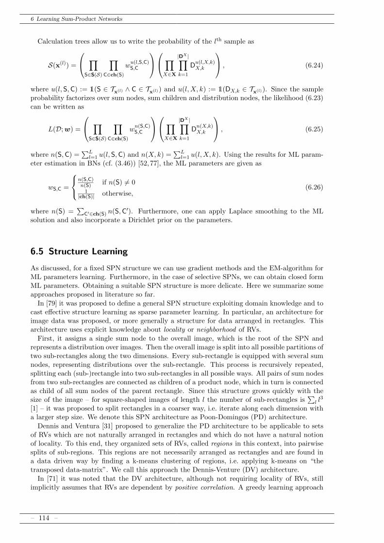
6 Learning Sum-Product Networks
Calculation trees allow us to write the probability of the lth sample as
S(x(l)) =
∏S∈S(S)
∏C∈ch(S)
wu(l,S,C)S,C
∏X∈X
|DX |∏k=1
Du(l,X,k)X,k
, (6.24)
where u(l,S,C) := 1(S ∈ Tx(l) ∧ C ∈ Tx(l)) and u(l,X, k) := 1(DX,k ∈ Tx(l)). Since the sampleprobability factorizes over sum nodes, sum children and distribution nodes, the likelihood (6.23)can be written as
L(D;w) =
∏S∈S(S)
∏C∈ch(S)
wn(S,C)S,C
∏X∈X
|DX |∏k=1
Dn(X,k)X,k
, (6.25)
where n(S,C) =∑L
l=1 u(l,S,C) and n(X, k) =∑L
l=1 u(l,X, k). Using the results for ML param-eter estimation in BNs (cf. (3.46)) [52,77], the ML parameters are given as
wS,C =
n(S,C)n(S) if n(S) 6= 0
1|ch(S)| otherwise,
(6.26)
where n(S) =∑
C′∈ch(S) n(S,C′). Furthermore, one can apply Laplace smoothing to the MLsolution and also incorporate a Dirichlet prior on the parameters.
6.5 Structure Learning
As discussed, for a fixed SPN structure we can use gradient methods and the EM-algorithm forML parameters learning. Furthermore, in the case of selective SPNs, we can obtain closed formML parameters. Obtaining a suitable SPN structure is more delicate. Here we summarize someapproaches proposed in literature so far.
In [79] it was proposed to define a general SPN structure exploiting domain knowledge and tocast effective structure learning as sparse parameter learning. In particular, an architecture forimage data was proposed, or more generally a structure for data arranged in rectangles. Thisarchitecture uses explicit knowledge about locality or neighborhood of RVs.
First, it assigns a single sum node to the overall image, which is the root of the SPN andrepresents a distribution over images. Then the overall image is split into all possible partitions oftwo sub-rectangles along the two dimensions. Every sub-rectangle is equipped with several sumnodes, representing distributions over the sub-rectangle. This process is recursively repeated,splitting each (sub-)rectangle into two sub-rectangles in all possible ways. All pairs of sum nodesfrom two sub-rectangles are connected as children of a product node, which in turn is connectedas child of all sum nodes of the parent rectangle. Since this structure grows quickly with thesize of the image – for square-shaped images of length l the number of sub-rectangles is
∑l l
3
[1] – it was proposed to split rectangles in a coarser way, i.e. iterate along each dimension witha larger step size. We denote this SPN architecture as Poon-Domingos (PD) architecture.
Dennis and Ventura [31] proposed to generalize the PD architecture to be applicable to setsof RVs which are not naturally arranged in rectangles and which do not have a natural notionof locality. To this end, they organized sets of RVs, called regions in this context, into pairwisesplits of sub-regions. This regions are not necessarily arranged as rectangles and are found ina data driven way by finding a k-means clustering of regions, i.e. applying k-means on “thetransposed data-matrix”. We call this approach the Dennis-Venture (DV) architecture.
In [71] it was noted that the DV architecture, although not requiring locality of RVs, stillimplicitly assumes that RVs are dependent by positive correlation. A greedy learning approach
– 114 –

6.5 Structure Learning
was proposed, merging regions of RVs from bottom-up instead of splitting regions from top-downas proposed in [31, 79]. Here the merging process is guided by independence tests and thus notrelying on positive correlation of the RVs.
In [40] a top-down scheme for learning SPN structures was proposed. They applied prob-abilistic clustering on data samples corresponding to sum nodes and clustering on RVs usingindependence tests, corresponding to product nodes. Thus, this approach also does not rely onpositive correlation of RVs.
In [84], the approach in [40] was refined in order to use input distributions over larger scopes.These input distributions are MNs represented as ACs [63].
In [72], a greedy hill-climbing algorithm was proposed to learn tree-shaped regular selectiveSPNs.
– 115 –


Foundations of Sum-Product Networks for Probabilistic Modeling
7Experiments and Applications
7.1 EM Algorithm
In Section 6.3 we derived the EM algorithm for sum-weights in SPNs (Algorithm 7). A correctlyderived EM algorithm must exhibit monotonicity, i.e. the log-likelihood must be non-decreasingin each iteration. To demonstrate monotonicity, we applied Algorithm 7 in a toy example. Weconsider sets of 9, 16 and 25 RVs, and construct SPNs using the PD architecture (cf. Section 6.5)by arranging the RVs in a 3×3, 4×4 and 5×5 array, respectively. We use K = 5 sum nodes perrectangle and G = 10 Gaussian PDFs as input distributions, whose means are set by histogramquantiles and whose standard deviations are uniformly set to 1 [31,71,79]. For each of the usedSPN structures, the number of sum nodes, sum-weights and product nodes, and the length ofthe longest path from the root node to some input distribution is shown in Table 7.1. As data we
Table 7.1: Statistics of toy SPN structures.
structure # sums #sum-weights #products longest path
3× 3 131 11600 2400 94× 4 416 39400 8000 105× 5 996 104200 21000 10
used 9, 16 and 25 randomly selected PCA features (among the first 100 features) of 1000 samplesfrom the MNIST data set, normalized to zero mean and unit variance. Furthermore, we addedwhite Gaussian noise with standard deviation 0.1. We initialized the sum-weights randomlyusing a Dirichlet distributions with uniform parameters α = 1, i.e. the uniform distribution onthe standard simplex. For each structure, we executed the EM algorithm for 100 iterations andperformed 10 random restarts, i.e. in total we ran the EM algorithm 30 times. Figure 7.1 showsthe log-likelihood of these runs, normalized by the number of RVs. We see that Algorithm 7indeed monotonously increases the training likelihood – in this experiment, the minimal increaseof log-likelihood within one iteration was 0.2.
– 117 –

7 Experiments and Applications
0 10 20 30 40 50 60 70 80 90 100−1520
−1510
−1500
−1490
−1480
−1470
−1460
−1450
−1440
−1430
−1420
3 × 3
4 × 4
5 × 5
Figure 7.1: Log-likelihood as a function of the EM iteration number.
7.2 MPE Inference
In Section 5.3, we discussed MPE inference and showed that Algorithm 5 delivers an MPEsolution for augmented SPNs. We further proposed Algorithm 6 which can be applied to theoriginal SPN but delivers an MPE solution for the augmented SPN. As a sanity check, weconstructed a toy SPN over 4 binary RVs and the corresponding augmented SPN, where MPEinference by exhaustive enumeration is tractable. To define the structure of our toy SPN, wearranged the 4 RVs as a 2×2 grid and used the PD architecture using 2 sum nodes per rectangle(cf. Section 6.5). This structure is shown in Figure 7.2(a). However, since this SPN regularlystructured, it does not fall prey to the low-depth bias and standard max-backtracking yields thesame solution as Algorithm 6. In order to demonstrate the low-depth bias, we add an additionalproduct node as child of the sum root node, whose children are IVs for each of the 4 RVs. Theresulting structure is shown in Figure 7.2(b).
We equipped this toy SPN with random sum-weights, drawn from a Dirichlet distributionwith uniform α-parameter, where α ∈ 0.5, 1, 2. Then we explicitly constructed the augmentedSPN using Algorithm 3, where we used uniform weights for the twin sums. The augmented SPNcontains 9 additional latent RVs, 8 with 4 states and 1 with 9 states.
We performed MPE inference by exhaustive enumeration in the augmented SPN, i.e. comput-ing the SPN distribution for all 9437184 possible inputs and selecting the max. We applied theback-tracking Algorithm 5 in the augmented SPN (denoted as BACK-AUG) and Algorithm 6in the original SPN (denoted as BACK-MPE). We also executed Algorithm 6 in the originalSPN, but with correction weights constantly set to 1, which corresponds to the back-trackingalgorithm in [79] (denoted as BACK-ORIG). Furthermore, we performed the sum approxima-tion of MPE (denoted as SUM, cf. Section 5.3). For each α, we repeated this experiment 100times. Table 7.2 shows the average/maximal deviation in log-probability from the exhaustiveMPE solution. A deviation of 0 means that the algorithm delivered an optimal solution, whilea negative value indicates a sub-optimal solution. We see that BACK-AUG and BACK-MPEalways delivered a correct MPE solution in this toy example, while BACK-ORIG and SUM donot guarantee an optimal solution. The minimum deviation was 0 for all algorithms in thisexample, i.e. all algorithms delivered a correct MPE solutions in some of the 100 runs.
Table 7.2: Results for MPE inference in toy SPN, comparing to exhaustive MPE solution.
BACK-AUG BACK-MPE BACK-ORIG SUM
α = 0.5 0.000/0.000 0.000/0.000 -0.533/-2.763 -0.183/-2.072
α = 1 0.000/0.000 0.000/0.000 -0.951/-2.680 -0.197/-1.675
α = 2 0.000/0.000 0.000/0.000 -1.415/-2.755 -0.168/-1.303
– 118 –
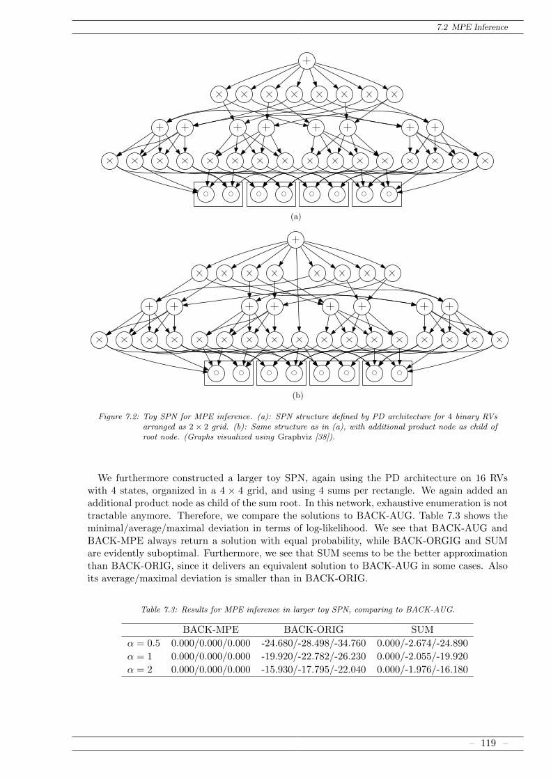
7.2 MPE Inference
(a)
(b)
Figure 7.2: Toy SPN for MPE inference. (a): SPN structure defined by PD architecture for 4 binary RVsarranged as 2 × 2 grid. (b): Same structure as in (a), with additional product node as child ofroot node. (Graphs visualized using Graphviz [38]).
We furthermore constructed a larger toy SPN, again using the PD architecture on 16 RVswith 4 states, organized in a 4 × 4 grid, and using 4 sums per rectangle. We again added anadditional product node as child of the sum root. In this network, exhaustive enumeration is nottractable anymore. Therefore, we compare the solutions to BACK-AUG. Table 7.3 shows theminimal/average/maximal deviation in terms of log-likelihood. We see that BACK-AUG andBACK-MPE always return a solution with equal probability, while BACK-ORGIG and SUMare evidently suboptimal. Furthermore, we see that SUM seems to be the better approximationthan BACK-ORIG, since it delivers an equivalent solution to BACK-AUG in some cases. Alsoits average/maximal deviation is smaller than in BACK-ORIG.
Table 7.3: Results for MPE inference in larger toy SPN, comparing to BACK-AUG.
BACK-MPE BACK-ORIG SUM
α = 0.5 0.000/0.000/0.000 -24.680/-28.498/-34.760 0.000/-2.674/-24.890
α = 1 0.000/0.000/0.000 -19.920/-22.782/-26.230 0.000/-2.055/-19.920
α = 2 0.000/0.000/0.000 -15.930/-17.795/-22.040 0.000/-1.976/-16.180
– 119 –

7 Experiments and Applications
7.3 Face Image Completion
In [79], it was demonstrated that MPE inference in SPNs achieves convincing results on theill-posed problem of image completion, i.e. reconstructing occluded parts of face images. To thisend, SPNs are trained on the ORL face image data set [86]. This data set consists of 400 faceimages, taken from 40 different persons, each with 10 images. The center 64× 64 region of theoriginal images was extracted9 and split into a training set of 35 persons (total 350 images) anda test set of 5 persons (total 50 images). We transformed the training images to zero mean andunit variance and applied the same transformation to the test images. We trained SPNs withthe method of Poon and Domingos (PD) [79], the method of Dennis and Ventura (DV) [31],and greedy-part-wise learning (Merge) [71]. We model single pixels with G Gaussian PDFs,where the means are set by the averages of histogram quantiles, and the standard deviation isuniformly set to 1. We set the number of Gaussians G = 10 for all three algorithms. All threealgorithms find a recursive decomposition of the overall image into sub-regions and each regionis equipped with K sum nodes, representing a dictionary of distributions over the respectiveregion. As in [31,79] we use K = 20 for all three algorithms.
In [31, 71, 79], SUM was used for reconstructing the missing image parts. As discussed inSection 5.3 and shown in the last section, this does not correspond to MPE-inference in theaugmented SPN. However, it is an arguable approximation for MPE inference in the originalSPN. Here, additionally to SUM we use BACK-MPE and BACK-ORIG, where the latter wasproposed in [79] for MPE inference. As discussed in Section 5.3, this corresponds to MPE-inference in the augmented SPN when using deterministic twin weights, which suffers from thelow-depth bias. As a base-line we replace missing pixel by the pixel values of the mean imageover all training images (MEAN).
Figures 7.3, 7.4, 7.5 and 7.6 show results for face image completion, when the left, top, rightand bottom halves of the images are missing, respectively. All models (PD, DV, Merge) and allinference methods (BACK-ORIG, SUM, BACK-MPE) perform reasonable for reconstructingmissing image parts. The artifacts introduced by BACK-ORIG seem to be often somewhatstronger than the artifacts introduced by SUM and BACK-MPE. Table 7.5 shows reconstructionSNRs for all models and all inference methods. BACK-ORIG consistently performs worse (oras well as) the other two methods. BACK-MPE and SUM are roughly on par. This observationis consistent with the remark in [79], that SUM performed better than BACK-ORIG in theexperiments. Note that MEAN consistently has the highest SNR. This probably comes fromthe artifacts with high energy produced by the SPN reconstructions.
Table 7.4 shows training and test log-likelihoods for models PD, DV and Merge. While Mergeachieves the lowest training likelihood, it achieves the highest likelihood on the test set, statingthat Merge generalized best in this task.
Table 7.4: Log-likelihoods on training and test set, normalized by number of samples.
Train Test
PD -4287.82 -5068.97DV -4356.41 -4673.73Merge -4493.46 -4667.04
9 Obtained from [78].
– 120 –

7.3 Face Image Completion
Original
Covered
MEAN
PD
︸︷︷
︸
BACK-ORIG
SUM
BACK-MPE
DV
︸︷︷
︸BACK-ORIG
SUM
BACK-MPE
Mer
ge
︸︷︷
︸
BACK-ORIG
SUM
BACK-MPE
Figure 7.3: Examples of face image reconstructions, left half is covered.
– 121 –

7 Experiments and Applications
Original
Covered
MEAN
PD
︸︷︷
︸
BACK-ORIG
SUM
BACK-MPE
DV
︸︷︷
︸BACK-ORIG
SUM
BACK-MPE
Mer
ge
︸︷︷
︸
BACK-ORIG
SUM
BACK-MPE
Figure 7.4: Examples of face image reconstructions, top half is covered.
– 122 –

7.3 Face Image Completion
Original
Covered
MEAN
PD
︸︷︷
︸
BACK-ORIG
SUM
BACK-MPE
DV
︸︷︷
︸BACK-ORIG
SUM
BACK-MPE
Mer
ge
︸︷︷
︸
BACK-ORIG
SUM
BACK-MPE
Figure 7.5: Examples of face image reconstructions, right half is covered.
– 123 –

7 Experiments and Applications
Original
Covered
MEAN
PD
︸︷︷
︸
BACK-ORIG
SUM
BACK-MPE
DV
︸︷︷
︸BACK-ORIG
SUM
BACK-MPE
Mer
ge
︸︷︷
︸
BACK-ORIG
SUM
BACK-MPE
Figure 7.6: Examples of face image reconstructions, bottom half is covered.
– 124 –

7.4 Artificial Bandwidth Extension
Table 7.5: Reconstruction SNRs for the top, bottom, left, and right halves of face images covered.
top bottom left right
MEAN – 13.16 11.25 12.72 11.83
PDBACK-ORIG 10.45 9.29 9.83 10.49
SUM 12.34 10.19 11.58 11.72BACK-MPE 12.61 10.20 11.56 11.77
DVBACK-ORIG 11.33 8.36 9.36 10.47
SUM 11.75 9.42 10.62 11.08BACK-MPE 11.33 9.58 11.29 10.70
MergeBACK-ORIG 10.64 8.88 9.40 9.83
SUM 12.43 9.83 10.96 11.78BACK-MPE 12.10 9.73 10.46 11.32
7.4 Artificial Bandwidth Extension
We can transfer their reconstruction abilities of SPNs to the audio domain, by considering animage-like representation of audio signal, e.g. the log-spectrogram. One problem which cantackled within this framework, is artificial bandwidth extension (ABE), i.e. to recover highfrequencies which are lost in telephone transmission. In [73], the HMM-based framework forABE [47,90] was modified to incorporate SPNs for modeling the observations.
In the HMM-based system [47], time signals are processed in frames with some overlap,yielding a total number of T frames. For each frame, the spectral envelope of the high-band ismodeled using cepstral coefficients obtained from linear prediction (LP). On a training set, thesecoefficients are clustered using the LBG algorithm [61]. The temporally ordered cluster indicesare used as hidden state sequence of an HMM, whose prior and transition probabilities can beestimated using the observed frequency estimates. For each hidden state, an observation GMMis trained on features taken from the low-band (see [47] for details about these features). Inthe test phase, the high frequency components and therefore the hidden states of the HMM aremissing. For each time frame, the marginal probability of the hidden state is inferred using theforward-backward algorithm [80]. For real-time capable systems, the backward-messages have tobe obtained from a limited number of Λ ≥ 0 look-ahead frames. Using the hidden state posterior,an MMSE estimate of the high-band cepstral coefficients is obtained [47], which together withthe periodogram of the low-band yield estimates of the wide-band cepstral coefficients. Toextend the excitation signal to the high-band, the low-band excitation is modulated either witha fixed frequency carrier, or with a pitch-dependent carrier. According to [47] and related ABEliterature, the results are quite insensitive to the method of extending the excitation.
To incorporate SPNs in HMM-based ABE, we use the log-spectra of the time frames asobservations, where redundant frequency bins are discarded. Let S(t, f) be the f th frequencybin of the tth time-frame of the full-band signal, t ∈ 1, . . . , T, f ∈ 1, . . . , F, where F is thenumber of frequency bins and St = (S(t, 1), . . . , S(t, F ))T . We cluster the log-spectra S1:T of training speech using the LBG algorithm, and use the cluster indices as hidden states ofan HMM. On each cluster, we train an SPN, yielding state-dependent models over the log-spectra. For training SPNs, we use the PD algorithm [79], requiring that the data is organizedas rectangular array; here the data is a 1 × F rectangular array. We used ρ = 20 sum nodesper rectangle and γ = 20 Gaussian PDF nodes per variable. This values were chosen as an“educated guess” and not cross-validated. Similar as in [79], we use a coarse resolution of 4,i.e. rectangles of height larger than 4 are split with a stepsize of 4.
For ABE we simulate narrow-band telephone speech [2] by applying a bandpass filter withstop frequencies 50 Hz and 4000 Hz. Let S(t, f) be the time-frequency bins of the telephonefiltered signal, and St = (S(t, 1), . . . , S(t, F ))T . Within the telephone band, we can assume that
– 125 –

7 Experiments and Applications
S(t, f) ≈ S(t, f), while some of the lowest and the upper half of the frequency bins in St are lost.To perform inference in the HMM, we marginalize missing data in the state-dependent SPNs,which can be done efficiently in SPNs, i.e. Gaussian distributions corresponding to unobservedfrequency bins, constantly return value 1, cf. Section 4.4. The output probabilities serve asobservation likelihoods and are processed by the forward-backward algorithm [80]. This deliversthe marginals p(Yt | et), where Yt is the hidden HMM variable in the the tth time frame, and etis denotes the observed data up to time frame t, i.e. all frequency bins in the telephone band,for all time frames 1, . . . , (t + Λ). An illustration of the modified HMM used in this paper isgiven in Figure 7.7, cf. also Figure 6.5.
??
?
?
YtYt 1- Yt 1+Yt 2- Yt 2+
??
?
?
??
?
?
??
?
?
??
?
?
St 2-
_
St 1-
_
St
_
St 1+
_
St 2+
_
Figure 7.7: Illustration of the HMM with SPN observation models. State-dependent SPNs are symbolized bytriangles with a circle on top. For the forward-backward algorithm, frequency bins marked with“?” (missing) are marginalized out by the SPNs.
We use the sum-approximation for MPE inference for recovering the missing spectrogramcontent, where we reconstruct the high-band only. Let St,k = (St,k(1), . . . St,k(F ))T be theMPE-reconstruction of the tth time frame, using the SPN depending on the kth HMM-state.Then we use the following bandwidth-extended log-spectrogram
S(t, f) =
S(t, f) if f < f ′∑K
k=1 p(Yt = k|et)St,k(f) o.w.(7.1)
where f ′ corresponds to 4000 Hz.
7.4.1 Reconstructing Time Signals
To synthesize a time-signal from the bandwidth extended log-spectrogram, we need to associate
a phase spectrum to the estimated magnitude spectrum eS(t,f). The problem of recoveringa time-domain signal given a modified magnitude appears in many speech applications, suchas single-channel speech enhancement [60], single-channel source separation [74, 92] and speechsignal modification [59,93]. These signal modifications are solely employed in spectral amplitudedomain while the phase information of the desired signal is not available. A typical approach isto use the observed (noisy) phase spectrum or to replace it with an enhanced/estimated phase.
In order to recover phase information for ABE, we use the iterative algorithm proposed byGriffin and Lim (GL) [42]. Let j ∈ 0, . . . , J be an iteration index, and C(j) be a complex
valued matrix generated in the jth iteration. Let |C(0)(t, f)| = eS(t,f) and
∠C(0)(t, f) =
∠C(f, t) 1 ≤ f ≤ f ′
0 o.w.,(7.2)
where C is the complex spectrogram of the bandpass filtered input signal. Within the telephoneband, phase information is considered reliable and copied from the input. Outside the narrow-band phase is initialized with zero. Note that in general C(0) is not a valid spectrogram since atime signal whose STFT equals C(0) might not exist. The jth iteration of the GL algorithm is
– 126 –

7.4 Artificial Bandwidth Extension
given by
C(j) = |C(0)| ⊗ ei∠G(C(j−1)), (7.3)
G(C) = STFT(STFT−1(C)), (7.4)
where ⊗ denotes the Hadamard product. At each iteration, the magnitude of the approximateSTFT C(j) is set to the magnitude |C(0)| estimated by the SPN while temporal coherence of thesignal is enforced by the operator G(·) (see e.g. [59] for more details). The estimated time signal
sj at the jth iteration is given by sj = STFT−1(C(j)
). At each iteration, the mean square
error between |STFT(sj)| and |C(0)| is reduced [42]. In our experiments, we set the number ofiterations J = 100, which appeared to be sufficient for convergence.
7.4.2 Experiments
We used 2 baselines in our experiments. The first baseline is the method proposed in [47],based on the vocal tract filter model using linear prediction. We used 64 HMM states and 16components per state-dependent GMM, which performed best in [47]. We refer as HMM-LPto this baseline. The second baseline is almost identical to our method, where we replaced theSPN with a Gaussian mixture model with 256 components with diagonal covariance matrices.For training GMMs, we ran the EM algorithm for maximal 100 iterations and using 3 randomrestarts. Since a GMM can be represented as an SPN with a single sum node, see Figure 6.8(b),inference using the GMM model works the same way as for SPNs. We refer as HMM-GMM tothis baseline. To the HMM incorporating SPNs as observation models, we refer as HMM-SPN.For HMM-GMM and HMM-SPN, we used the same clustering of log-spectra using a codebooksize of 64.
We used time-frames of 512 samples length, with 75% overlap, which using a sampling fre-quency of 16 kHz corresponds to a frame length of 32 ms and a frame rate of 8 ms. Before applyingthe FFT, the frames were weighted with a Hamming window. For the forward-backward algo-rithm we used a look-ahead of Λ = 3 frames, which corresponds to the minimal delay introducedby the 75% frame-overlap. We performed our experiments on the GRID corpus [21], where weused the test speakers with numbers 1, 2, 18, and 20, referred to as s1, s2, s18, and s20, respec-tively. Speakers s1 and s2 are male, and s18 and s20 are female. We trained speaker dependentand speaker independent models. For speaker dependent models we used 10 minutes of speech ofthe respective speaker. For speaker independent models we used 10 minutes of speech obtainedfrom the remaining 30 speakers of the corpus, each speaker providing approximately 20 secondsof speech. For testing we used 50 utterances per test speaker, not included in the training set.
(a) Original (b) HMM-LP (c) HMM-GMM (d) HMM-SPN
Figure 7.8: Log-spectrogram of the utterance “Bin green at zed 5 now”, spoken by s18. (a): original fullbandwidth signal. (b): ABE result of HMM-LP [47]. (c): ABE result of HMM-GMM. (d): ABEresults of HMM-SPN.
Figure 7.8 shows log-spectrograms of a test utterance of speaker s18 and the bandwidth ex-tended signals by HMM-LP, HMM-GMM and HMM-SPN, using speaker dependent models. We
– 127 –

7 Experiments and Applications
see that HMM-LP succeeds in reconstructing a harmonic structure for voiced sounds. However,we see that fricative and plosive sounds are not well captured. The reconstruction by HMM-GMM is blurry and does not recover the harmonic structure of the original signal well, butpartly recovers high-frequency content related to consonants. The HMM-SPN method recoversa natural high frequency structure, which largely resembles the original full-band signal: theharmonic structure appears more natural than the one delivered by HMM-LP and consonantsounds seem to be better detected and reconstructed than by HMM-GMM.
For an objective evaluation, we use the log-spectral distortion (LSD) in the high-band [47].Given an original signal and an ABE reconstruction, we perform Lth-order LPC analysis foreach frame, where L = 9. This yields (L + 1)-dimensional coefficient vectors at and at of theoriginal and the reconstructed signals, respectively. The spectral envelope modeled by a genericLPC coefficient vector a = (a0, . . . , aL)t is given as
Ea(ejΩ) =σ
|∑L
k=0 ake−jkΩ|
, (7.5)
where σ is the square-root of the variance of the LPC-analyzed signal. The LSD for the τ th
frame, in high-band is calculated as
LSDτ =
√∫ πν (20 logEaτ (ejΩ)− 20 logEaτ (ejΩ))2 dΩ
π − ν, (7.6)
where ν = π 4000fs/2 , fs being the sampling frequency. The LSD at utterance level is given as the
average of LSDτ over all frames. Tables 7.6 and 7.7 show the LSD of all three methods for thespeaker dependent and speaker independent scenarios, respectively, averaged over the 50 testsentences. We see a clear ranking of the three methods, and that the HMM-SPN method alwaysperforms best. All differences are significant at a 0.95 confidence level, according to a pairedone-sided t-test.
Table 7.6: Average LSD using speaker-dependent models.
s1 s2 s18 s20
HMM-LP 7.13 7.57 6.48 6.41HMM-GMM 3.18 2.93 2.28 2.82HMM-SPN 3.12 2.84 2.15 2.59
Table 7.7: Average LSD using speaker-independent models.
s1 s2 s18 s20
HMM-LP 7.12 7.66 6.60 6.34HMM-GMM 3.62 4.46 3.82 3.60HMM-SPN 3.42 3.85 3.05 3.36
– 128 –

Foundations of Sum-Product Networks for Probabilistic Modeling
8Discussion and Future Work
The core part of this thesis is dedicated to investigate the foundations of SPNs and to strengthenour theoretic understanding about them. We want to summarize the most important insightsand draw a conceptional picture of SPNs, yielding from the results developed in this thesis.
In the most basic definition, SPNs are feedforward neural networks containing sum and prod-uct neurons. We define a distribution by simply normalizing the output of the SPN. Althoughthis approach is mathematically sound, we will not be able to perform inference in such a model,except in the simplest cases. This calls for considering a restricted class of SPNs, which allowsat least to compute the normalization constant of the SPN. In [79], this class was called validSPNs, and two sufficient conditions were given to guarantee validity: completeness and consis-tency. At the same time, an alternative condition to consistency, decomposability, was given;decomposability implies consistency, but not vice versa, i.e. consistency is the weaker condition.However, in literature mostly decomposability is used, since decomposability is conceptuallyeasier and also easier to establish. This raises the question: Do we loose much when using de-composability? The answer we give here is no, since consistent SPNs can not model distributionssignificantly more concise than decomposable SPNs (Theorem 4.3). Furthermore, consistencyrules out a class of inference scenarios defined via the differential approach [27], which can beapplied in decomposable SPNs. These arguments give us license to consider only complete anddecomposable SPNs, simplifying our conceptual image of SPNs.
SPNs with locally normalized weights are readily normalized, and in literature often locallynormalized SPNs were used due to convenience. Again, this raises the question: Do we loosemuch by this restriction? Here the answer is an even clearer no; we can without loss of generalityassume locally normalized SPN weights (Theorem 4.2), which again simplifies our conceptualimage of SPNs.
Complete and decomposable SPNs can be easily generalized be replacing IVs by more generalinput distributions, also over larger scopes. It is immediate that generalized SPNs representsome distribution and it is clear how to evaluate this distribution for some sample. However,it was missed in literature to carry over other inference mechanism from finite-state SPNs,i.e. marginalization and the differential approach. In this thesis we derived these inferencescenarios for generalized SPNs, cf. Section 4.4. When we neglect consistency, we see that finite-state SPNs are indeed just a special case of generalized SPNs. Furthermore, since we canalways assume locally normalized weights, we see that SPNs can be understood as nothingbut a nested arrangement of mixtures of distributions (sum nodes) and factorized distributions(product nodes). Although this description of SPNs sounds simple, one must not underestimatetheir model power. We saw in Section 6.4, that even a quite restricted class of SPNs, i.e. regular
– 129 –
8 Discussion and Future Work
selective SPNs, generalizes BNs over finite-state RVs and incorporates advanced concepts suchas context-specific independence, nested multi-nets and sub-component sharing, without needfor any specialized inference mechanism.
A central theme of SPNs is their interpretation as hierarchical structured latent RV model.As pointed out in Chapter 5, the original augmentation of SPNs explicitly incorporating theselatent RVs is too simplistic, leading to irritating results. We completed this augmentation, byintroducing the so-called twin sum nodes. Furthermore, we introduced an IMAP of the aug-mented model, represented as BN, linking SPNs back to classical PGMs. The BN interpretationof augmented SPNs helped us to derive a sound EM-algorithm for SPN weights.
The latent RV interpretation was already used in the seminal paper [79] for data reconstructionusing MPE inference. The used algorithm for MPE inference was never shown to be correct,besides the fact that the latent model was not completely specified. We showed that it is indeeda correct algorithm for augmented SPNs, but that it needs a modification when applied tonon-augmented SPNs.
Furthermore, so far it was not clear if the more desirable MAP inference for data reconstruc-tion can be performed efficiently in SPNs. We gave a negative result, showing that this problemis generally NP-hard.
This thesis tries to shed some light on the foundations of SPNs. However, it is certainly notan exhaustive or completely rigorous treatment of the subject of SPNs. Many questions areopen and we want to conclude the thesis with possible future research topics.
• What is the complexity of MAP inference in SPNs?
• Is there a class of SPNs for which MAP inference can efficiently be solved, i.e. its decisionversion is in P?
• If yes, how does it look like?
• Design an algorithm which returns a MAP solution given enough time and memory andwhich delivers a solution with sub-optimality bounds, i.e. an any-time solution. A possibletechnique could be branch-and-bound.
• What are suitable cost functions for learning SPNs?
• Given such cost function, is learning SPNs NP-hard? (Presumably yes)
• Given a budget of arithmetic operations and a cost function, design an algorithm returninga globally optimal SPN.
– 130 –

Foundations of Sum-Product Networks for Probabilistic Modeling
AAppendix
A.1 Proofs for Chapter 4
Proposition 4.1. Let P be a product node and Y be its shared RVs. P is consistent if and onlyif for each Y ∈ Y there exists a unique y∗ ∈ val(Y ) with λY=y∗ ∈ desc(P).
Proof of Proposition (4.1).
Direction “⇐”, i.e. suppose for each Y ∈ Y there exists a unique y∗ ∈ val(Y ) with λY=y∗ ∈desc(P). Consider arbitrary two distinct children C′,C′′ ∈ ch(P) and let Y′ = sc(C′) ∩ sc(C′′),where from Definition 4.12 (shared RVs) it follows that Y′ ⊆ Y. First, let X ∈ sc(C′) \ Y′
arbitrary. Since X /∈ sc(C′′), we have
λX=x ∈ desc(C′)⇒ ∀x′ : λX=x′ /∈ desc(C′′), (A.1)
and in particular
λX=x ∈ desc(C′)⇒ ∀x′ 6= x : λX=x′ /∈ desc(C′′). (A.2)
Now let X ∈ Y′ arbitrary. Since X ∈ Y, there is a unique x∗ ∈ val(X) with λX=x∗ ∈ desc(C′)and λX=x∗ ∈ desc(C′′), and again (A.2) holds. Since C′, C′′ and X are arbitrary, P is consistent.
Direction “⇒”, i.e. suppose P is consistent. If Y is empty, i.e. P is decomposable, then theclaimed property holds trivially for all Y. Otherwise let Y ∈ Y arbitrary and let C′ and C′′
be arbitrary two children having Y in their scope. There are at least two such children byDefinition 4.12 (shared RVs). There must be a unique y∗ with λY=y∗ ∈ desc(C′) and λY=y∗ ∈desc(C′′). To see this, note that there must be at least one y′ ∈ val(Y ) with λY=y′ ∈ desc(C′)and at least one y′′ ∈ val(Y ) with λY=y′′ ∈ desc(C′′), since Y is in the scope of both C′ and C′′.However, there can be at most one such y′ and y′′. Assume there were y′1 and y′2, y′1 6= y′2. Theneither for y′ = y′1 or for y′ = y′2 we had a contradiction to
λY=y′ ∈ desc(C′)⇒ ∀y′′ 6= y′ : λY=y′ /∈ desc(C′′). (A.3)
i.e. P would not be consistent. By symmetry, there is also at most one y′′, and (A.3) can onlyhold when y′ = y′′ =: y∗. Therefore, since Y , C′ and C′′ are arbitrary, there must be a uniquey∗ with y∗ ∈ desc(C), ∀C ∈ ch(P) : Y ∈ sc(C). Therefore, this y∗ is also the unique value withλY=y∗ ∈ desc(P).
– 131 –
A Appendix
Lemma 4.1. Let N be a node in some complete and consistent SPN, X ∈ sc(N) and x ∈ val(X).When λX=x /∈ desc(N), then ∀x ∈ val(X) with x[X] = x we have N(x) = 0.
Proof of Lemma 4.1.
When N = λX=x′ , for some x′ ∈ val(X), the lemma clearly holds, since x′ 6= x.
When N is a product or a sum, let N = N′ ∈ desc(N) : X ∈ sc(N′). Let K = |N| and letN1, . . . ,NK be a topologically order list of N, i.e. Nk /∈ desc(Nl) when k > l. We can assumethat for some I, N1, . . . ,NI are IVs of X, NI+1, . . . ,NK are sum and product nodes, whereNK = N. For any x ∈ val(X) with x[X] = x, we have N1(x) = N2(x) = · · · = NI(x) = 0, sinceλX=x /∈ desc(N).
When all N1(x) = N2(x) = · · · = Nk(x) = 0 for some k ≥ I, then also Nk+1(x) = 0. WhenNk+1 is a sum node, due to completeness, all children of Nk+1 must have X in their scope. Thismeans that all children are in N1, . . . ,Nk. Therefore Nk+1(x) = 0. When Nk+1 is a product,at least on child has to be in N1, . . . ,Nk. Therefore Nk+1(x) = 0. Thus, by induction, for allN′ ∈ N we have N′(x) = 0. In particular this is true for NK = N.
Lemma 4.2. Let P be a PMF over X and Y ⊆ X, Z = X \ Y such that there exists ay∗ ∈ val(Y) with P (z,y) = 0 when y 6= y∗. Then we have P (z,y) = 1(y = y∗)P (z).
Proof of Lemma 4.2.
Since P (z,y) = 0 when y 6= y∗, P (z) =∑
y∈val(Y) P (z,y) = P (z,y∗). Thus
P (z,y) =
0 if y 6= y∗
P (z) if y = y∗= 1(y = y∗)P (z). (A.4)
Proposition 4.2. A complete and decomposable SPN computes the network polynomial of someunnormalized distribution.
Proof of Proposition 4.2.
Recall that a network polynomial for unnormalized distribution Φ is defined as (cf. (4.13)):
fΦ(λ) =∑
x∈val(X)
Φ(x)∏X∈X
λX=x[X]. (A.5)
Assume some topological order of the SPN nodes. We show by induction over this order, frombottom to top, that each sub-SPN SN computes a network polynomial over sc(N). The basisare the IVs λX=x which compute
λX=x =∑
x′∈val(X)
1(x′ = x)λX=x′ , (A.6)
which has the form (A.5), i.e. IVs compute network polynomials.
– 132 –

A.1 Proofs for Chapter 4
A complete sum node S computes
S(λ) =∑
C∈ch(S)
wS,C C(λ) (A.7)
=∑
C∈ch(S)
wS,C
∑x∈val(sc(S))
ΦC(x)∏
X∈sc(S)
λX=x[X] (A.8)
=∑
x∈val(sc(S))
∑C∈ch(S)
wS,C ΦC(x)
∏X∈sc(S)
λX=x[X] (A.9)
=∑
x∈val(sc(S))
ΦS(x)∏
X∈sc(S)
λX=x[X], (A.10)
where ΦC is the unnormalized distributions of the network polynomial of C, and ΦS(x) :=∑C∈ch(S)wS,C ΦC(x). In (A.8) we apply the induction hypothesis and the fact that for complete
sum nodes the scopes of the node and all its children are the same. We see that (A.10) has theform (A.5), i.e. the induction step holds for complete sum nodes.
Now consider some decomposable product node P with children ch(P) = C1, . . . ,CK. Theproduct node P computes
P(λ) =K∏k=1
Ck(λ) (A.11)
=
K∏k=1
∑xk∈val(sc(Ck))
ΦCk(xk)∏
X∈sc(Ck)
λX=xk[X] (A.12)
=∑
x1∈val(sc(C1))
· · ·∑
xK∈val(sc(CK))
K∏k=1
ΦCk(xk)∏
X∈sc(Ck)
λX=xk[X]
(A.13)
=∑
x∈val(sc(P))
(K∏k=1
ΦCk(x[sc(Ck)])
) ∏X∈sc(P)
λX=x[X]
(A.14)
=∑
x∈val(sc(P))
ΦP(x)∏
X∈sc(P)
λX=x[X], (A.15)
where ΦCk is the distributions of the network polynomial of Ck, and ΦP(x) :=∏Kk=1 ΦCk(x[sc(Ck)]).
In (A.12) we use the induction hypothesis, in (A.13) we apply the distributive law, and in (A.14)we use the fact that the scope of a decomposable product node is partitioned by the scopes ofits children. We see that (A.15) has the same form as (A.5), i.e. the induction step holds forcomplete product nodes.
Consequently, each sub-SPN and therefore also the overall SPN computes a network polyno-mial of some unnormalized distribution.
Proposition 4.3. Every complete and consistent, but non-decomposable SPT S = ((V,E),w)over X can be transformed into a complete and decomposable SPT S ′ = ((V′,E′),w′) over Xsuch that S ≡ S ′, and where |V′| ≤ |V|, AS′ ≤ AS and MS′ < MS .
Proof. For SPTs, no links are introduced in steps 2–7 of Algorithm 2. Consider a non-decomposableproduct P in the SPT, and let Y be the shared RVs. If sc(P) = Y, the whole sub-SPNrooted at P will be replaced by
∏Y ∈Y λY=y∗[Y ] in step 13. The deleted sub-SPN computes∏
Y ∈Y(λY=y∗[Y ])kY , where kY are integers with kY ≥ 1, and at least one kY > 1, since other-
wise P would be decomposable. Thus, replacing this sub-SPN by the decomposable product instep 13 saves at least one multiplication.
– 133 –

A Appendix
Similarly, when sc(P) 6= Y, steps 21–23 prune nodes from the sub-SPN rooted at P, cor-responding to the computation of
∏Y ∈Y(λY=y∗[Y ])
kY with kY ≥ 1, and at least one kY > 1.This requires at least one multiplication more than directly connecting λY=y∗[Y ] to P in step24. Clearly, steps 17–20 are never performed in SPTs, since no N ∈ desc(P) \ P can have aparent outside the descendants of P.
Thus, for every non-decomposable product, Algorithm 2 saves at least one multiplication.
Proposition 4.5. Let S be an SPN and Sg be its gated SPN. Then
1. Sg is an SPN over X ∪ Z.
2. S(X) = Sg(X) =∑
z∈val(Z) Sg(X, z).
3. For any X ∈ X and k ∈ 1, . . . , |DX |, let XD = sc(DX,k) and XR = X \XD. It holdsthat
Sg(X, ZX = k,Z \ ZX) = DX,k(XD)Sg(XR, ZX = k,Z \ ZX), (A.16)
i.e.
XD ⊥⊥ XR ∪ Z \ ZX |ZX (A.17)
In particular
Sg(X, ZX = k) = DX,k(XD)Sg(XR, ZX = k), (A.18)
Proof of Proposition 4.5.
ad 1) In the gated SPN, each distribution node D is replaced by a product node with scopesc(D) ∪ ZX | X ∈ sc(D). That is, in the scope of each ancestor of D, an RV X isreplaced by a compound RV X,ZX. This leaves completeness and decomposabilityintact. The products introduced in (4.65) are also clearly decomposable and the IVsare input distributions over the DSs. Therefore Sg fulfills Definition 4.15, i.e. it is angeneralized SPN, and the scope of the root is X ∪ Z.
ad 2) Since Sg is a generalized SPN over X∪Z, marginalization over Z is performed by settingall λZX=k = 1. In this case, the introduced product nodes simply copy the correspondinginput distribution, i.e. all remaining nodes in Sg perform the same computations as in S,so their outputs agree.
ad 3) Consider all internal nodes N in Sg which have X in their scope. Since they have X in theirscope, they also have ZX in their scope. Consider a fixed k and assume ZX = k. We split Ninto two sets N′ and N′′, where ∀N ∈ N′ : DX,k ∈ desc(N) and ∀N ∈ N′′ : DX,k 6∈ desc(N).
We first show by induction that all N ∈ N′′ output 0. Let N1, . . . ,NK be a topologi-cal ordered list of nodes in N′′, i.e. k > l ⇒ Nk /∈ desc(Nl). We assume w.l.o.g. thatN1, . . . ,N|DX |−1, are the gates PX,l, l 6= k. These nodes output 0, since λZX=l = 0 forZX = k. This is the induction basis. For the induction step, assume that N1, . . . ,NM out-put 0, for |DX | − 1 ≤M < K. We show that then also NM+1 outputs 0. If NM+1 is a sumS, all its children must also be in N′′: they must be in N, i.e. have X in their scope, sinceS has X in its scope. They also can not be N′, since otherwise S would be in N′. Thusthey are in N′′, and furthermore they must be in N1, . . . ,NM, due to the topologicalordering. Since they output 0, also S outputs 0. Similarly, when NM+1 is a product P, itmust have exactly one child with X in its scope, which must be in N1, . . . ,NM. Sincethis child outputs 0 also P outputs 0. Therefore all N′′ output 0.
– 134 –

A.2 Proofs for Chapter 5
We now show by induction that all N ∈ N′ have the form
DX,k(XD)N(XR′ , ZX = k,Z′ \ ZX), (A.19)
where XR′ = XR ∩ sc(N) and Z′ = Z ∩ sc(N). Let N1, . . . ,NK be a topological orderedlist of nodes in N′, i.e. k > l ⇒ Nk /∈ desc(Nl). N1 must be the gate PX,k which has theform DX,k
∏Y ∈sc(DX,k) λZY =[DX,k]Y , which has the form (A.19) with XR′ = ∅. This is the
induction basis. For the induction step, assume that all N1, . . . ,NM have the form (A.19),for M ≥ 1. We show that then also NM+1 has the form (A.19). When NM+1 is a sum nodeS, all its children must be contained in N due to completeness and since X is in sc(S).Partition ch(S) into C′ = ch(S) ∩N′ and C′′ = ch(S) ∩N′′. C′ must contain at least onenode, since S is contained in N′. Furthermore, C′ must be a subset of N1, . . . ,NM, dueto the topological ordering. S computes
S(X, ZX = k,Z′) =∑C∈C′
wS,CDX,k(XD)C(XR′ , ZX = k,Z′ \ ZX) +
∑C∈C′′
wS,C 0
(A.20)
= DX,k(XD)∑C∈C′
wS,C C(XR′ , ZX = k,Z′ ZX), (A.21)
which has the form (A.19). When NM+1 is a product node P it must have exactly one childC in N′, due to decomposability and since P is in N′. This C also must be in N1, . . . ,NM,due to the topological ordering. The product node computes
P(X, ZX = k,Z′) = DX,k(XD)C(·, ZX = k,Z′ ∩ sc(C) \ ZX)∏
C′∈ch(P)\C
C′(·),
(A.22)
which has the form (A.19). Therefore all N′ have this form. Since the root is contained inN′, the claimed property (4.66) follows. Eq. (4.68) follows by marginalizing Z \ ZX.
A.2 Proofs for Chapter 5
Proposition 5.1. Let S be an SPN over X, S ′ = aug(S) and Z := ZS(S). Then S ′ is acomplete and decomposable SPN over X ∪ Z with S ′(X) ≡ S(X).
Proof of Proposition 5.1. We restate Algorithm 3 in Algorithm 8. If S ′ is a complete and de-composable SPN over X ∪ Z, then S ′(X) ≡ S(X) is immediate: In this case, computing S ′(x)for any x ∈ val(X) is done by marginalizing Z, i.e. setting all λZS=k = 1. Introducing the linksclearly does not change the function computed by the SPN. Also connecting λZS=k to PkS doesnot change the function, when λZS=k is set constantly to 1. The twin sum S also constantlyoutputs 1, and therefore does not change the computed function when connected to the links ofits conditioning sums Sc. Therefore, the outputs of S and S ′ agree for each x ∈ val(X) when Zis marginalized in S ′, i.e. S ′(X) ≡ S(X).
It remains to show that S ′ is complete, decomposable and totally normalized, and that itsroot has X ∪ Z in its scope. After the first part of Algorithm 3 the SPN is clearly completeand decomposable, but does not have any ZS in its scope. We show that after each executionof the for-loop body (10 − 21), the SPN remains complete, decomposable and contains ZS inits root’s scope. After step 12, the links PkS are clearly decomposable, because no λZS=k has
– 135 –

A Appendix
Algorithm 8 Augment SPN S∀S ∈ S(S), ∀k ∈ 1, . . . ,KS let wS,k = wS,CkS
, wS,k = wS,CkS
Introduce links:1: for S ∈ S(S) do2: for k = 1 . . .KS do3: Introduce a new product node PkS in S4: Disconnect CkS from S5: Connect CkS as child of PkS6: Connect PkS as child of S with weight wS,k
7: end for8: end for
Introduce IVs and twins:9: for S ∈ S(S) do
10: for k ∈ 1, . . . ,KS do11: Connect new IV λZS=k as child of PkS12: end for13: if Sc(S) 6= ∅ then14: Introduce a twin sum node S in S15: ∀k ∈ 1, . . . ,KS: connect λZS=k as child of S, and let wS,λZS=k
= wS,k
16: for Sc ∈ Sc(S) do17: for k ∈ k | S 6∈ desc(PkSc) do18: Connect S as child of PkSc19: end for20: end for21: end if22: end for
been connected to any other node in the SPN before. Since PkS are reachable from the root,also λZS=k are reachable, i.e. ZS is now in the scope of the root. Since S was complete beforestep 12, i.e. all links had the same scope, it remains complete after step 12. The scopes of allancestors of S are now augmented by Z, which could corrupt decomposability and complete-ness of the ancestors. However, there can be no non-decomposable ancestors: if there was anon-decomposable product node it must have Z in the scope of at least two children. Thiswould imply that S is reachable from both children, contradicting that the product node wasdecomposable beforehand. However, in general there can be incomplete sum nodes as illustratedin Figure 5.2. These are treated in steps 13− 21:
The twin sum S, if introduced, is clearly complete and has scope Z. Furthermore, incom-pleteness of any conditioning sum Sc can only be caused by links not having ZS in their scope.The scope of these links is augmented by ZS in step 18. These links remain decomposable andmoreover, Sc is rendered complete now. These operations do not affect the scope of any furtherancestor of Sc, since their scope already contains Z. Therefore, the SPN remains complete anddecomposable, and adds ZS into the root’s scope. Finally, it is easy to see that all sum nodeshave normalized weights, i.e. S ′ is a complete, decomposable and locally normalized SPN overX ∪ Z.
Proposition 5.2. Let S be an SPN over X, Y ⊆ ZS(S) and Z = ZS(S) \Y. Let y ∈ val(Y)and let S ′ = aug(S). It holds that
1. Each node in Sy has the same scope as its corresponding node in S ′.
– 136 –

A.2 Proofs for Chapter 5
Algorithm 9 Configure SPN
1: Sy ← aug(S)2: for Y ∈ Y do3: for y ∈ val(Y ), y 6= y[Y ] do4: Delete λY=y and link PySY5: end for6: end for7: Delete all nodes in Sy which are not reachable from the root
2. Sy is a complete and decomposable SPN over X ∪Y ∪ Z.
3. For any node N in Sy with sc(N) ∩Y = ∅, we have that SyN = S ′N.
4. For y′ ∈ val(Y) it holds that
Sy(X,Z,y′) =
S ′(X,Z,y′) if y′ = y
0 otherwise(A.23)
Proof of Proposition 5.2. We restate Algorithm 4 in Algorithm 9.
ad 1.) We show that 1. holds after each iteration of the main for-loop (steps 3–6) of Algorithm 9.In each iteration, IVs λY=y are disconnected and links PySY are deleted for y 6= y[Y ].Clearly, this can only change the scopes of their ancestors. The direct ancestors SY and
SY still have the same scope, since they are left with one child, either Py[Y ]SY
or λY=y[Y ].
Any further ancestor is an ancestor of SY or SY . Since the scopes of SY or SY remain thesame, also the scopes of these ancestors remain the same.
ad 2.) The graph of Sy is rooted and acyclic, since the root can not be a link and deletingnodes and edges can not introduce cycles. When an IV λY=y is deleted, also the link PySYis deleted, so no internal nodes are left as leaves. The roots in Sy and aug(S) are the same,and by point 1., X∪Y∪Z is the scope of the root. Sy is also complete and decomposable:After each iteration of the main for-loop (steps 3–6), SY and SY are trivially complete,
since they are left with a single child. Py[Y ]SY
is also clearly decomposable. Completeness or
decomposability of any ancestor of SY or SY is left intact, since SY or SY do not changetheir scopes.
ad 3.) According to 1., the scope of N in S ′ and Sy is the same. Since sc(N) ∩ Y = ∅, thedisconnected IVs and deleted links are no descendants of N, i.e. no descendants of N aredisconnected in the for-loop (steps 3–6) in Algorithm 9. Since N is present in Sy, it mustbe still reachable from the root after Algorithm 9. Therefore also all descendants of N arereachable, i.e. Sy
N = S ′N.
ad 4.) When the input for S ′ is fixed to x, z,y, all disconnected IVs λY=y and deleted links PySYwould evaluate to zero. The outputs of SY and SY are therefore the same in S ′ and Sy.All other ancestors of λY=y and PySY are ancestors of SY or SY , i.e. their outputs also arethe same. This includes the root and therefore Sy(x, z,y) = S ′(x, z,y), for any x, z.
When y′ 6= y, then there must be a Y ∈ Y such that the IV λY=y′[Y ] can not be reachedfrom the root. Thus, with Lemma 4.1 it follows that if y′ 6= y, then Sy(x, z,y′) = 0.
Lemma 5.1. Let S be an SPN over X, let S be a sum node in S and Z = ZancS(S)\S. Forany z ∈ val(Z), the configured SPN Sz contains either S or its twin S, but not both.
– 137 –

A Appendix
Proof of Lemma 5.1. Sz must contain either S or S, since ZS is in the scope of the root byProposition 5.2 and any IV related to ZS can be reached only via S or S. To show that notboth are in Sz, let Πk denote the set of paths of length k from the root to any node N withZS ∈ sc(N). A path in Πk is denoted as (N1, . . . ,Nk), cf. Section 2.2. For k > 1, all paths inΠk can be constructed by extending all paths in Πk−1, i.e. each path in Πk−1 is extended byall children of the path’s last node. Let K be the smallest number such that there is a path inΠk containing S or S.
We show by induction, that |Πk| = 1, k = 1, . . . ,K. Note that Π1 contains a single path (N),where N is the root, therefore the induction basis holds.
For the induction step, we show that given |Πk−1| = 1, then also |Πk| = 1. Let (N1, . . . ,Nk−1)be the single path in Πk−1. If Nk−1 is a product node, then it has a single child C with ZS ∈ sc(C),due to decomposability. If Nk−1 is a sum node, then it must be in ancS(S) \ S, and thereforehas a single child in the configured SPN. Therefore, there is a single way to extend the path andtherefore |Πk| = 1, k = 1, . . . ,K. This single path does either lead to S or S. Since S /∈ desc(S)and S /∈ desc(S), Sz contains a single path to one of them, but not to both.
A.3 Proofs for Chapter 6
Lemma 6.1. For each complete, decomposable and selective SPN S and each sample x, Tx is atree.
Proof of Lemma 6.1. For each node N in Tx there exists a calculation path Πx(N) in S bydefinition. We have to show that this path is unique. Suppose there were two distinct calculationpaths Πx(N) = (N1, . . . ,NJ) and Π′x(N) = (N′1, . . . ,N
′J ′). Since all calculation paths start at the
root, there must be a smallest j such that Nj = N′j , Nj+1 6= N′j+1 and N ∈ desc(Nj+1) ∧ N ∈desc(N′j+1). Such Nj does not exist: if Nj is a product node, N ∈ desc(Nj+1)∧N ∈ desc(N′j+1)contradicts decomposability. If Nj is a sum node, it would contradict selectivity, since Nj+1(x) >0 and N′j+1(x) > 0. Therefore each calculation path is unique, i.e. Tx is a tree.
– 138 –

Foundations of Sum-Product Networks for Probabilistic Modeling
References
[1] “OEIS Foundation Inc. (2011), The On-Line Encyclopedia of Integer Sequences,http://oeis.org/A000537.”
[2] “ETSI: Digital cellular telecommunications system (phase 2+); Enhanced full rate (EFR)speech transcoding, ETSI EN 300 726 V8.0.1,” Nov. 2000.
[3] J. Aczel, Lectures on Functional Equations and their Applications. Academic Press, 1966.
[4] M. R. Amer and S. Todorovic, “Sum-Product Networks for Modeling Activities withStochastic Structure,” in Proceedings of CVPR, 2012, pp. 1314–1321.
[5] S. Arnborg and Sjordin, “On the foundations of Bayesianism,” in Bayesian Inference andMaximum Entropy Methods in Science and Engineering, 20th International Workshop,A. Mohammad-Djarafi, Ed., 2001, pp. 61–71.
[6] P. Billingsley, Probability and Measure. Wiley-Interscience, 1995.
[7] C. M. Bishop, Pattern Recognition and Machine Learning, 1st ed. Springer, Oct. 2007.
[8] H. L. Bodlaender, F. van den Eijkhof, and L. C. van der Gaag, “On the complexity of theMPA problem in probabilistic networks,” in Proceedings of the 15th European Conferenceon Artificial Intelligence, 2002, pp. 675–679.
[9] V. I. Bogachev, Measure Theory. Springer Berlin Heidelberg New York, 2007, vol. I andII.
[10] C. Boutilier, N. Friedman, M. Goldszmidt, and D. Koller, “Context-Specific Independencein Bayesian Networks,” in UAI, 1996.
[11] W. Buntine, “Theory Refinement on Bayesian Networks,” in Uncertainty in ArtificialIntelligence (UAI), 1991, pp. 52–60.
[12] H. Chan and A. Darwiche, “When do numbers really matter?” JAIR, vol. 17, pp. 265–287,2002.
[13] ——, “Sensitivity analysis in Bayesian networks: From single to multiple parameters.” inUAI, 2004, pp. 67–75.
[14] W. C. Cheng, S. Kok, H. V. Pham, H. L. Chieu, and K. M. A. Chai, “Language Modelingwith Sum-Product Networks,” in Proceedings of Interspeech, 2014.
[15] D. M. Chickering, “Learning Bayesian Networks is NP-Complete,” in Learning from Data:Artificial Intelligence and Statistics V. Springer-Verlag, New York, 1996, pp. 121–130.
[16] ——, “Learning Equivalence Classes of Bayesian-Network Structures,” Journal of MachineLearning Research, vol. 2, pp. 445–498, 2002.
[17] D. M. Chickering, D. Geiger, and D. Heckerman, “Learning Bayesian Networks is NP-hard,” Technical Report No. MSR-TR-94-17, Microsoft Research, Redmond, Washington,Tech. Rep., 1994.
– 139 –

References
[18] ——, “Learning Bayesian networks: Search methods and experimental results,” in Proc.of Fifth Conference on Artificial Intelligence and Statistics, 1995, pp. 112–128.
[19] D. M. Chickering and D. Heckerman, “A Bayesian approach to learning Bayesian networkswith local structure,” in UAI, 1997, pp. 80–89.
[20] C. K. Chow and C. N. Liu, “Approximating Discrete Probability Distributions with De-pendence Trees,” in IEEE Transactions on Information Theory, vol. 14, no. 3, 1968, pp.462–467.
[21] M. Cooke, J. Barker, S. Cunningham, and X. Shao, “An audio-visual corpus for speechperception and automatic speech recognition,” J. Acoust. Soc. Amer., vol. 120, pp. 2421–2424, Nov 2005.
[22] G. F. Cooper and E. Herskovits, “A Bayesian Method for the Induction of ProbabilisticNetworks from Data,” Machine Learning, vol. 9, pp. 309–347, 1992.
[23] R. Cowell, Introduction to inference for Bayesian networks. in Learning in GraphicalModels, (M.I. Jordan, editor), MIT Press, 1999.
[24] R. Cowell, A. Dawid, S. Lauritzen, and D. Spiegelhalter, Probabilistic networks and expertsystems. Springer, 1999.
[25] R. Cox, “Probability, frequency, and reasonable expectation,” American Journal ofPhysics, vol. 14, pp. 1–13, 1946.
[26] A. Darwiche, “A logical approach to factoring belief networks,” in Proceedings of KR,2002, pp. 409–420.
[27] ——, “A Differential Approach to Inference in Bayesian Networks,” ACM, vol. 50, no. 3,pp. 280–305, 2003.
[28] C. de Campos, Z. Zeng, and Q. Ji, “Structure learning of Bayesian networks using con-straints,” in International Conference on Machine Learning (ICML), 2009, pp. 113–120.
[29] B. de Finetti, Foresight: Its Logical Laws, Its Subjective Sources, H. E. Kyburg and H. E. K.Smokler, Eds. Robert E. Kreiger Publishing Co, 1937.
[30] A. Dempster, N. Laird, and D. Rubin, “Maximum likelihood from incomplete data via theEM algorithm,” J. Royal Statistical Society, Series B, vol. 39, no. 1, pp. 1–38, 1977.
[31] A. Dennis and D. Ventura, “Learning the Architecture of Sum-Product Networks UsingClustering on Variables,” in Advances in Neural Information Processing Systems 25, 2012,pp. 2042–2050.
[32] D. Dubois and H. Prade, Possibility Theory: an Approach to Computerized Processing ofUncertainty, 1988.
[33] J. Duchi, S. Shalev-Shwartz, Y. Singer, and T. Chandra, “ Efficient Projections onto theL1-Ball for Learning in High Dimensions,” in ICML, 2008.
[34] G. Elidan and N. Friedman, “Learning the dimensionality of hidden variables,” in Proc.17th Conference on Uncertainty in Artificial Intelligence, 2001.
[35] ——, “Learning Hidden Variable Networks: The Information Bottleneck Approach,” Jour-nal of Machine Learning Research, vol. 6, pp. 81–127, 2005.
– 140 –

References
[36] G. Elidan, N. Lotner, N. Friedman, and D. Koller, “Discovering Hidden Variables: AStructure-Based Approach,” in Neural Information Processing Systems. MIT Press, 2001,pp. 479–485.
[37] N. Friedman, “The Bayesian structural EM algorithm,” in Proc. 14th Conference on Un-certainty in Artificial Intelligence, 1998, pp. 129–138.
[38] E. R. Gansner and S. C. North, “An open graph visualization system and its applications tosoftware engineering,” SOFTWARE - PRACTICE AND EXPERIENCE, vol. 30, no. 11,pp. 1203–1233, 2000.
[39] R. Gens and P. Domingos, “Discriminative Learning of Sum-Product Networks,” in Ad-vances in Neural Information Processing Systems 25, 2012, pp. 3248–3256.
[40] ——, “Learning the Structure of Sum-Product Networks,” Proceedings of ICML, pp. 873–880, 2013.
[41] F. Glover, “Heuristics for Integer Programming using Surrogate Constraints,” DecisionSciences, vol. 8, no. 1, pp. 156–166, 1977.
[42] D. Griffin and J. Lim, “Signal estimation from modified short-time Fourier transform,”IEEE Transactions on Acoustics, Speech and Signal Processing, vol. 32, no. 2, pp. 236–243,1984.
[43] J. Halpern, “A counterexample to theorems of Cox and Fine,” Journal of Artificial Intel-ligence Research, vol. 10, pp. 67–85, 1999.
[44] D. Heckerman, D. Geiger, and D. M. Chickering, “Learning Bayesian Networks: TheCombination of Knowledge and Statistical Data,” Machine Learning, vol. 20, pp. 197–243, 1995.
[45] T. Jaakkola, D. Sontag, A. Globerson, and M. Meila, “Learning Bayesian Network Struc-ture using LP Relaxations,” in AI Statistics, 2010, pp. 358–365.
[46] M. Jaeger, J. Nielsen, and T. Silander, “Learning probabilistic decision graphs ,” Interna-tional Journal of Approximate Reasoning, vol. 42, pp. 84–100, 2006.
[47] P. Jax and P. Vary, “On artificial bandwidth extension of telephone speech,” Signal Pro-cessing, vol. 83, pp. 1707–1719, 2003.
[48] E. T. Jaynes, Probability Theory: The Logic of Science. Cambridge University Press,2003.
[49] F. Jensen, An introduction to Bayesian networks. UCL Press Limited, 1996.
[50] D. Kisa, G. V. den Broeck, A. Choi, and A. Darwiche, “Probabilistic Sentential DecisionDiagrams,” in KR, 2014.
[51] M. Koivisto and K. Sood, “Exact Bayesian Structure Discovery in Bayesian Networks,”Journal of Machine Learning Research, vol. 5, pp. 549–573, 2004.
[52] D. Koller and N. Friedman, Probabilistic Graphical Models: Principles and Techniques.MIT Press, 2009.
[53] B. Kosko, “Fuzziness vs. Probability,” International Journal of General Systems, vol. 17,pp. 211–240, 1990.
– 141 –

References
[54] J. Kwisthout, “Most Probable Explanations In Bayesian Networks: Complexity AndTractability ,” International Journal of Approximate Reasoning, vol. 52, pp. 1452–1469,2011.
[55] W. Lam and F. Bacchus, “Learning Bayesian belief networks: an approach based on theMDL principle,” Computational Intelligence, vol. 10, no. 3, pp. 269–293, 1994.
[56] H. Langseth and T. Nielsen, “Latent Classification Models,” Machine Learning, vol. 59,pp. 237–265, 2005.
[57] ——, “Classification using Hierarchical Naıve Bayes models,” Machine Learning, vol. 63,pp. 135–159, 2006.
[58] S. Lauritzen and D. Spiegelhalter, “Local computations with probabilities on graphicalstructures and their application to expert systems,” J. Royal Statistical Society B, vol. 50,pp. 157–224, 1988.
[59] J. Le Roux, “Exploiting Regularities in Natural Acoustical Scenes for Monaural AudioSignal Estimation, Decomposition, Restoration and Modification,” Ph.D. dissertation, TheUniversity of Tokyo & Universite Paris, 2009.
[60] C. Leitner and F. Pernkopf, “Speech Enhancement Using Pre-Image Iterations,” inICASSP, 2012, pp. 4665–4668.
[61] Y. Linde, A. Buzo, and R. Gray, “An algorithm for vector quantizer design,” IEEE Trans-action on Communication, vol. 28, no. 1, pp. 84–95, 1980.
[62] H.-A. Loeliger, “An Introduction to Factor Graphs,” IEEE Signal Processing Magazine,vol. 21, no. 1, pp. 28–41, 2004.
[63] D. Lowd and A. Rooshenas, “Learning Markov Networks with Arithmetic Circuits,” Pro-ceedings of AISTATS, pp. 406–414, 2013.
[64] D. Lowd and P. Domingos, “Learning Arithmetic Circuits,” in Twenty Fourth Conferenceon Uncertainty in Artificial Intelligence, 2008, pp. 383–392.
[65] R. Neal and G. Hinton, “A view of the EM algorithm that justifies incremental, sparse,and other variants,” in Learning in Graphical Models. Cambridge, MA: MIT Press, 1999,pp. 355–368.
[66] C. Papadimitriou, Computational Complexity. Addison-Wesley, 1994.
[67] J. Paris, The Uncertain Reasoner’s Companion. Cambridge University Press, 1994.
[68] J. D. Park, “MAP Complexity Results and Approximation Methods,” in Proceedings ofthe Conference on Uncertainty in Artificial Intelligence, 2002, pp. 338–396.
[69] J. D. Park and A. Darwiche, “Complexity Results and Approximation Strategies for MAPExplanations ,” Journal of Artificial Intelligence Research, vol. 21, pp. 101–133, 2004.
[70] J. Pearl, Probabilistic Reasoning in Intelligent Systems: Networks of Plausible Inference.San Francisco, CA, USA: Morgan Kaufmann Publishers Inc., 1988.
[71] R. Peharz, B. Geiger, and F. Pernkopf, “Greedy Part-Wise Learning of Sum-ProductNetworks,” in ECML/PKDD, vol. 8189. Springer Berlin, 2013, pp. 612–627.
[72] R. Peharz, R. Gens, and P. Domingos, “Learning Selective Sum-Product Networks,” inICML-LTPM Workshop, 2014.
– 142 –

References
[73] R. Peharz, G. Kapeller, P. Mowlaee, and F. Pernkopf, “Modeling Speech with Sum-Product Networks: Application to Bandwidth Extension,” in Proceedings of ICASSP,2014.
[74] R. Peharz, M. Stark, and F. Pernkopf, “A Factorial Sparse Coder Model for Single ChannelSource Separation,” in Interspeech, 2010, pp. 386–389.
[75] R. Peharz, S. Tschiatschek, F. Pernkopf, and P. Domingos, “On Theoretical Properties ofSum-Product Networks,” in Proceedings of AISTATS, 2015.
[76] R. Peharz and F. Pernkopf, “Exact Maximum Margin Structure Learning of BayesianNetworks,” in ICML, 2012.
[77] F. Pernkopf, R. Peharz, and S. Tschiatschek, Introduction to Probabilistic Graphical Mod-els, ser. Academic Press Library in Signal Processing. Elsevier, 2013, vol. 1, ch. 18.
[78] H. Poon and P. Domingos, “http://alchemy.cs.washington.edu/spn/,” 2011, (online).
[79] ——, “Sum-Product Networks: A New Deep Architecture,” in Proceedings of the Twenty-Seventh Conference on Uncertainty in Artificial Intelligence, 2011, pp. 337–346.
[80] L. Rabiner, “A tutorial on hidden Markov models and selected applications in speechrecognition,” in Proceedings of the IEEE, vol. 77, no. 2, 1989, pp. 257–286.
[81] M. Ratajczak, S. Tschiatschek, and F. Pernkopf, “Sum-Product Networks for StructuredPrediction: Context-Specific Deep Conditional Random Fields.” in ICML-LTPM Work-shop, 2014.
[82] J. Rissanen, “Modeling by shortest data description,” Automatica, vol. 14, pp. 465–471,1978.
[83] R. W. Robinson, “Counting labeled acyclic digraphs,” in New Directions in the Theory ofGraphs, F. Harary, Ed. Academic Press, NY, 1973, pp. 239–273.
[84] A. Rooshenas and D. Lowd, “Learning Sum-Product Networks with Direct and IndirectVariable Interactions,” ICML – JMLR W&CP, vol. 32, pp. 710–718, 2014.
[85] J. S. Rosenthal, A first look at rigorous probability theory, 2nd ed. World Scientific, 2006.
[86] F. Samaria and A. Harter, “Parameterisation of a Stochastic Model for Human FaceIdentification,” in Proceedings of the 2nd IEEE Workshop on Applications of ComputerVision, 1994, pp. 138–142.
[87] G. Shafer, A Mathematical Theory of Evidence. Princeton University Press, 1976.
[88] T. Silander and P. Myllymaki, “A simple approach for finding the globally optimalBayesian network structure,” in UAI, 2006, pp. 445–452.
[89] A. P. Singh and A. W. Moore, “Finding optimal Bayesian networks by dynamic program-ming,” Carnegie Mellon University, Tech. Rep., 2005.
[90] G.-B. Song and P. Martynovich, “A study of HMM-based bandwidth extension of speechsignals,” Signal Processing, vol. 89, pp. 2036–2044, 2009.
[91] P. Spirtes, C. Glymour, and R. Scheines, Causation, Prediction, and Search. MIT Press,2000.
– 143 –

References
[92] M. Stark, M. Wohlmayr, and F. Pernkopf, “Source-Filter based Single Channel SpeechSeparation using Pitch Information,” IEEE Transactions on Audio, Speech and LanguageProcessing, vol. 19, no. 2, pp. 242–255, 2011.
[93] N. Sturmel and L. Daudet, “Signal reconstruction from STFT magnitude: a state of theart,” pp. 375–386, 2011.
[94] J. Suzuki, “A construction of Bayesian networks from databases based on an MDL prin-ciple,” in UAI, 1993, pp. 266–273.
[95] ——, “Learning Bayesian Belief Networks based on the minimum description length prin-ciple: An efficient algorithm using the B&B technique,” in Int. Conference on MachineLearning, 1996, pp. 462–470.
[96] M. Teyssier and D. Koller, “Ordering-Based Search : A Simple and Effective Algorithmfor Learning Bayesian Networks,” in Proc. 21st Conference on Uncertainty in ArtificialIntelligence, vol. 51, 2005, pp. 584–590.
[97] S. Tschiatschek, P. Reinprecht, M. Muecke, and F. Pernkopf, “Bayesian Network Classifierswith Reduced Precision Parameters,” in ECML PKDD, 2012.
[98] K. S. Van Horn, “Constructing a logic of plausible inference: a guide to Cox’s theorem,”International Journal of Approximate Reasoning, pp. 3–24, 2003.
[99] T. Verma and J. Pearl, “An algorithm for deciding if a set of observed independencies hasa causal explanation, ,” in UAI, 1992.
[100] G. Vitali, Sul problema della misura dei gruppi di punti di una retta. Tip. Gamberini eParmeggiani, 1905.
[101] H. Wettig, P. Grunwald, T. Roos, P. Myllymaki, and H. Tirri, “When discriminativelearning of Bayesian network parameters is easy,” in International Joint Conferences onArtificial Intelligence (IJCAI), 2003, pp. 491–496.
[102] N. Zhang, “Hierarchical Latent Class Models for Cluster Analysis,” Journal of MachineLearning Research, vol. 5, pp. 697–723, 2004.
[103] N. Zhang, T. Nielsen, and F. Jensen, “Latent variable discovery in classification models,”Artificial Intelligence in Medicine, vol. 30, pp. 283–299, 2004.
– 144 –

Foundations of Sum-Product Networks for Probabilistic Modeling
List of Publications
[1] Robert Peharz, Sebastian Tschiatschek, Franz Pernkopf and Pedro Domingos. On Theo-retical Properties of Sum-Product Networks. In Proceedings of AISTATS, 2015.
[2] Robert Peharz, Robert Gens, and Pedro Domingos. Learning Selective Sum-Product Net-works. In ICML Workshop on Learning Tractable Probabilistic Models, 2014.
[3] Robert Peharz, Georg Kapeller, Pejman Mowlaee, and Franz Pernkopf. Modeling Speechwith Sum-Product Networks: Application to Bandwidth Extension. In Proceedings ofICASSP, pages 3699–3703, 2014.
[4] Robert Peharz, Bernhard Geiger, and Franz Pernkopf. Greedy part-wise learning of sum-product networks. In Proceedings of ECML/PKDD, 2013.
[5] Franz Pernkopf, Robert Peharz, and Sebastian Tschiatschek. Introduction to ProbabilisticGraphical Models. Chapter 18 in E-Reference Signal Processing. Elsevier, 2013.
[6] Robert Peharz, Sebastian Tschiatschek, and Franz Pernkopf. The most generative maxi-mum margin Bayesian networks. In Proceedings of ICML, pages 235–243, 2013.
[7] Robert Peharz and Franz Pernkopf. Exact maximum margin structure learning of Bayesiannetworks. In Proceedings of ICML, 2012.
[8] Robert Peharz and Franz Pernkopf. On linear and mixmax interaction models for singlechannel source separation. In Proceedings of ICASSP, pages 249–252, 2012.
[9] Robert Peharz and Franz Pernkopf. Sparse nonnegative matrix factorization with `0-constraints. Neurocomputing, 80:38–46, 2012.
[10] Robert Peharz, Michael Wohlmayr, and Franz Pernkopf. Gain-robust multi-pitch trackingusing sparse nonnegative matrix factorization. In Proceedings of ICASSP, pages 5416–5419,2011.
[11] Michael Wohlmayr, Robert Peharz, and Franz Pernkopf. Efficient implementation of prob-abilistic multi-pitch tracking. In Proceedings of ICASSP, pages 5412–5415, 2011.
[12] Robert Peharz, Michael Stark, and Franz Pernkopf. A factorial sparse coder model forsingle channel source separation. In Proceedings of Interspeech, 386–389, 2010.
[13] Robert Peharz, Michael Stark, and Franz Pernkopf. Sparse nonnegative matrix factorizationusing `0-constraints. In Proceedings of MLSP, 83–88, 2010.
– 145 –