On Sum Coloring and Sum Multi-Coloring for

Restricted Families of Graphs ⋆

Allan Borodin, Ioana Ivan, Yuli Ye, and Bryce Zimny

Department of Computer Science, University of Toronto,Toronto, ON, Canada M5S 3G4,

{bor,y3ye,zimny}@cs.toronto.eduioana.ivan@utoronto.ca

Abstract. We consider the sum coloring (chromatic sum) and summulti-coloring problems for restricted families of graphs. In particular, weconsider the graph classes of proper intersection graphs of axis-parallelrectangles, proper interval graphs, and unit disk graphs. All the abovementioned graph classes belong to a more general graph class of (k + 1)-clawfree graphs (respectively, for k = 4, 2, 5).We prove that sum coloring is NP-hard for penny graphs and unit squaregraphs which implies NP-hardness for unit disk graphs and proper in-tersection graphs of axis-parallel rectangles. We show a 2-approximationalgorithm for unit square graphs, with the assumption that the geo-metric representation of the graph is given. For sum multi-coloring, weconfirm that the greedy first-fit coloring, after ordering vertices by theirdemands, achieves a k-approximation for the preemptive version of summulti-coloring on (k + 1)-clawfree graphs. Finally, we study priority al-gorithms as a model for greedy algorithms for the sum coloring and summulti-coloring problems. We show various inapproximation results underseveral natural input representations.

1 Introduction

The sum coloring problem (SC), also known as the chromatic sum problem, wasformally introduced in [4]. For a given graph G = (V, E), a proper coloring ofG is an assignment of positive integers to its vertices φ : V → Z+ such thatno two adjacent vertices are assigned the same color. The sum coloring problemseeks a proper coloring such that the sum of colors over all vertices

∑v∈V φ(v) is

minimized. Sum coloring has many applications in job scheduling and resourceallocation. Consider an instance of job scheduling in which one is given a setS of jobs, each requiring unit execution time. We construct the conflict graphG whose vertex set is in one-to-one correspondence with the set of input jobsS, and an edge exists between two vertices if and only if the correspondingjobs conflict for resources. Dividing the chromatic sum of the conflict graphG = (V, E) by n = |V | then determines the minimum average job completion

⋆ This work was supported by the Natural Sciences and Engineering Research Councilof Canada and the Department of Computer Science, University of Toronto.

time. Throughout this paper we will let n (respectively, m) denote the number ofvertices (respectively the number of edges) in the input graph being considered.

The sum coloring problem has been studied extensively in the literature. Theproblem is NP-hard for general graphs [4], and cannot be approximated withinn1−ǫ for any ǫ > 0 unless ZPP=NP [5][7]. The problem is polynomial timesolvable for proper interval graphs [9] and trees [4]; however, it is APX-hard forboth bipartite graphs [6] and interval graphs [11]. The best known approximationalgorithm for interval graphs has approximation ratio 1.796 [16] and for bipartitegraphs the best known is a 27

26 -approximation [12].One well-studied extension of the sum coloring problem is sum multi-coloring

(SMC): given graph G = (V, E) and a demand function x : V → {1, 2, ...},color each vertex v with x(v) different colors so as to minimize the sum ofthe maximum color assigned to each vertex while assigning distinct colors toadjacent vertices. That is, a coloring is now an assignment φ : V → 2Z+

suchthat |φ(v)| = x(v) for all v, and φ(u)∩φ(v) = ∅ for all (u, v) ∈ E. There are twovariants to the sum multi-coloring problem, namely the non-preemptive version(npSMC) where colors assigned to each vertex must be consecutive integers andthe preemptive version (pSMC) in which colors need not be consecutive. Oneinteresting fact about pSMC and npSMC is that there is a known polynomialtime algorithm that solves npSMC for trees [13], while pSMC remains NP-hardfor trees [14]. This is in contrast to other graph classes (see [19]) where theknown approximation for pSMC is better than that for npSMC and also incontrast to the results in [10] that reduce pSMC to the weighted MIS problem,suggesting that npSMC is in general a harder problem. For a more completereview of previous results on sum coloring and sum multi-coloring, see [19].

In this paper, we consider the sum coloring and sum multi-coloring problemfor restricted families of graphs with respect to both hardness and approximationalgorithms. We shall always assume that the graph is connected since otherwiseeach connected component can be colored separately. The remainder of the paperis organized as follows. In Section 2, we discuss various classes of (k+1)-clawfreegraphs. We prove the problem is NP-hard for penny graphs and unit squaregraphs, and show a 2-approximation for unit square graphs in Section 3. Westudy the sum multi-coloring problem for (k + 1)-clawfree graphs in Section 4and priority inapproximations in Section 5. Section 6 concludes with some openproblems.

2 (k + 1)-Clawfree Graphs

A graph is (k +1)-clawfree if every vertex has at most k independent neighbors.We follow the notation in [22] and let G(ISk) denote the class of (k+1)-clawfreegraphs. Similarly, we let G(V CCk) denote the class of graphs for which theneighborhood of every vertex has a clique cover of size at most k. It is easy tosee that G(V CCk) is a subset of G(ISk).

It turns out many interesting families of geometric intersection graphs are inthe class G(V CCk) and hence in the class of G(ISk) for a small parameter k.

2

– Proper Interval Graphs and Proper Circular Arc Graphs: The vertices areintervals on the real line (respectively, arcs on a circle). Two vertices areadjacent if the two intervals (reps. arcs) intersect. The properness conditionstates that no interval (arc) is properly contained inside another interval(arc). Since the containment is proper, for any given interval (arc), any in-tersecting interval (arc) must intersect at one of its two end points. Thereforethese graphs are in G(V CC2).

– Proper Intersection Graphs of Axis-Parallel Rectangles: The vertices are axis-paralel rectangles. Two vertices are adjacent if the two rectangles intersect.Properness means that if rectangle R1 interescts rectangle R2 then the pro-jection of R1 (onto either the x or y-axis) is not properly contained in theprojection of R2. That is, the projection of the rectangles onto either the x ory axis becomes a proper interval graph. Since the containment is proper, fora given rectangle, every intersecting rectangle intersects it at one of its fourcorners. Therefore the underlying graph is in G(V CC4). A special case iswhen the rectangles are axis parallel translates of a fixed axis parallel graph.In the case of translates of of a unit square, ther resulting graphs are calledunit square graphs.

Fig. 1. Proper Circular Arc Graphs and Proper Intersection of Rectangles

– Unit Disk Graphs: The vertices are disks of unit size and two vertices areadjacent if the two disks intersect each other (including the boundary). Forany disk, there are at most five pair-wise non-intersecting disks intersecting asingle disk. Therefore the underlying graph is in G(IS5). For any given unitdisk, we can partition its conflicting region into six sectors so that any twounit disks whose centers lying in the same sector must intersect; see Figure 3below. Therefore unit disk graphs are in G(V CC6). It is not hard to showthat this bound is tight; i.e., unit disk graphs are not in G(V CC5). This givesa natural example which separates G(V CC5) and G(IS5). A special case ofunit disk graphs is penny graphs where two disks cannot have a commoninterior point and two vertices are adjacent if the two disks touch each otherat the boundary.

3

Fig. 2. Penny Graphs and Unit Disk Graphs

Fig. 3. Unit Disk Graphs are in G(V CC6)

– Intersection of k-Sets: The vertices are sets Si of elements from some universewith |Si| ≤ k, and Si and Sj are adjacent if and only if Si ∩ Sj 6= ∅. These

graphs are in G(V CCk).

– Line Graphs: The vertices are edges of an underlying graph and two verticesare adjacent if they share a common vertex in the underlying graph. It is easyto see that for a particular edge, it can have at most two non-intersectingedges intersect with it. Therefore, line graphs are in G(V CC2).

With the exception of unit disk graphs, all the examples of (k + 1)-clawfreegraphs given are in the subclass G(V CCk). However, we note that G(V CCk) is asubstantially different class of graphs than G(ISk). In fact, based on a variationof Mycielski’s construction [1], we can show that for every k, there is a 3-clawfreegraph that is not in G(V CCk). We also note that for fixed k, determining if G isin G(ISk) can clearly be decided in time nk+2 whereas it is NP-hard to determinemembership in G(V CCk) for k ≥ 3.

4

3 Sum Coloring for Unit Square Graphs

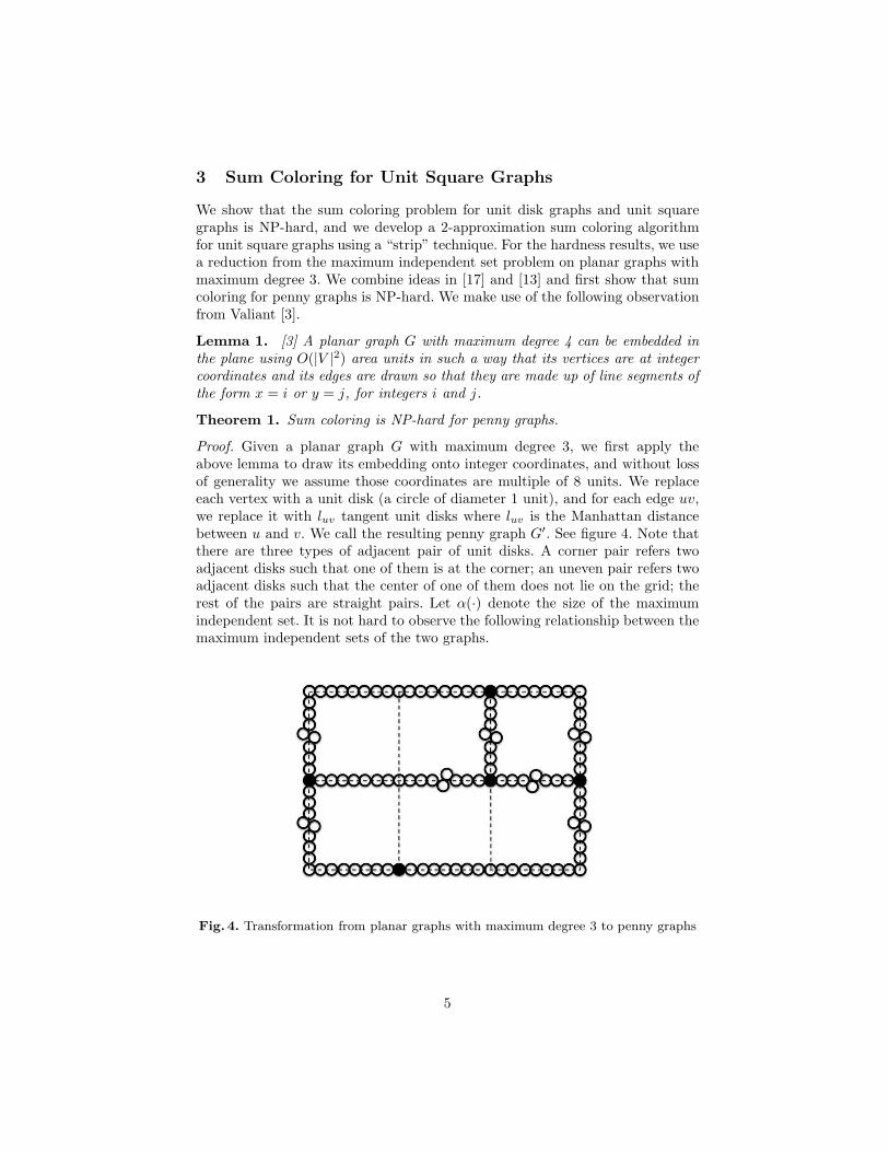
We show that the sum coloring problem for unit disk graphs and unit squaregraphs is NP-hard, and we develop a 2-approximation sum coloring algorithmfor unit square graphs using a “strip” technique. For the hardness results, we usea reduction from the maximum independent set problem on planar graphs withmaximum degree 3. We combine ideas in [17] and [13] and first show that sumcoloring for penny graphs is NP-hard. We make use of the following observationfrom Valiant [3].

Lemma 1. [3] A planar graph G with maximum degree 4 can be embedded inthe plane using O(|V |2) area units in such a way that its vertices are at integercoordinates and its edges are drawn so that they are made up of line segments ofthe form x = i or y = j, for integers i and j.

Theorem 1. Sum coloring is NP-hard for penny graphs.

Proof. Given a planar graph G with maximum degree 3, we first apply theabove lemma to draw its embedding onto integer coordinates, and without lossof generality we assume those coordinates are multiple of 8 units. We replaceeach vertex with a unit disk (a circle of diameter 1 unit), and for each edge uv,we replace it with luv tangent unit disks where luv is the Manhattan distancebetween u and v. We call the resulting penny graph G′. See figure 4. Note thatthere are three types of adjacent pair of unit disks. A corner pair refers twoadjacent disks such that one of them is at the corner; an uneven pair refers twoadjacent disks such that the center of one of them does not lie on the grid; therest of the pairs are straight pairs. Let α(·) denote the size of the maximumindependent set. It is not hard to observe the following relationship between themaximum independent sets of the two graphs.

Fig. 4. Transformation from planar graphs with maximum degree 3 to penny graphs

5

Lemma 2. α(G′) = α(G) +∑

uv∈Eluv

2 .

Proof. We first show that α(G′) is at least α(G)+∑

uv∈Eluv

2 . Given a maximumindependent set I of G, then for any edge uv, at least one of u and v are not in I,hence we can add luv

2 alternating disks for each edge uv to form an independent

set of G′. Therefore, α(G′) ≥ α(G) +∑

uv∈Eluv

2 . On the other hand, given amaximum independent set I ′ of G′, we can do the following modifications to I ′

without changing the size of I ′. For each edge uv in G, if both u and v are in I ′,then the number of disks along the edge uv which are in I ′ must be less thanluv

2 , we can then remove, say v, from I ′ and increase the number of disks alongthe edge uv which are in I ′ by at least one. We keep doing that until for anyedge uv in G there is at most one vertex in I ′.

It is clear that after such modification, the vertices in I ′∩G is an independentset for G, and hence α(G′) ≤ α(G) +

∑uv∈E

luv

2 . ⊓⊔We now do a second transformation. For each straight pair of adjacent unit

disks, we do a transformation as shown in Fig. 5; for each uneven pair of adjacentunit disks, we do a transformation as shown in Fig. 6 and for each corner pairof adjacent unit disks, we do a transformation as shown in Fig. 7.

Fig. 5. Transformation for straight pairs

The purpose of the second transformation is that for each edge uv in G′, wewant to add an edge gadget as shown in Fig 8. Because the original graph is aplanar graph with maximum degree 3, we can add these edge gadget in such away that there are no overlapping disks and two disks in different gadgets donot touch each other. We call the resulting graph G′′. Let m be the the numberof edges in G′′ and n the number of vertices, let SC(G′′) denote its chromaticsum. We now prove the following lemma to complete the reduction.

Lemma 3. SC(G′′) = 8m + 2n − α(G′).

Proof. We first show that the chromatic sum of G′′ is at most 8m+2n−α(G′). Tosee that we give an explicit coloring of G′′. Let I be the maximum independent

6

Fig. 6. Transformation for uneven pairs

Fig. 7. Transformation for corner pairs

Fig. 8. The edge gadget

7

set of G′, we coloring all vertices in I with color 1. We then color the remainingvertices in G′ with color 2. Consider an edge gadget as depicted in figure 8. Sinceat least one of u and v is colored with 2, without loss of generality, assume u hascolor 2. We then color y with 1, z with 3, x with 2 and p, q with 1. Thereforethe chromatic sum of G′′ is at most 8m + 2n − α(G′).

We now show the chromatic sum of G′′ is at least 8m + 2n− α(G′). Assumean optimal sum coloring, we first claim that all vertices in G′ colored with 1 mustform an independent set of G′. Suppose this is not the case and assume both u

and v are colored with 1. There are two cases, the best possible choices of colorslead to Fig. 9 and 10, which achieves the sum of 13 and 12 respectively. If werecolor v with 2, we achieves the sum 11 as show in Fig. 11. However, recoloringv might lead to recoloring its other adjacent edge gadgets. We claim that we cancoloring every other edge gadgets adjacent to v to maintain at least its originalsum. Let u′ be any other vertex adjacent to v in G′, and y′, z′, x′, p′, q′ be thecorresponding vertices in the gadget, there are two cases:

Fig. 9. Recoloring case 1

Fig. 10. Recoloring case 2

1. If u′ is not colored with 2, then color z′ with 1, y′ with 2, x′ with 3, p′, q′

with 1. This is the minimum possible, so it cannot exceed the original.2. If u′ is colored with 2, then color z′ with 1, y′ with 3, x′ with 2, p′, q′ with

1. This is also the minimum possible, so it cannot exceed the original.

8

Fig. 11. Result coloring

Therefore by recoloring v with 2 and proper recoloring its neighborhood gadgets,we reduce the total sum, hence, all vertices in G′ colored with 1 must form anindependent set of G′. For the remaining vertices in G′, we at least color themwith 2 and for each gadgets, 8 is the best possible. Therefore the chromatic sumis at most 8m + 2n − α(G′). ⊓⊔

The NP-hardness follows immediately from Lemma 1, 2 and 3.⊓⊔

It follows immediately that sum coloring is NP-hard for unit disk graphs,since the class of penny graphs is a subclass of unit disk graphs.

Corollary 1. Sum coloring is NP-hard for unit disk graphs.

The transformation in the reduction to penny graphs also works for unitsquare graphs with a slight modification, i.e., by using unit squares instead ofunit disks throughout the proof.

Theorem 2. Sum coloring is NP-hard for unit square graphs.

Since polynomial-time optimal algorithms are unlikely, we seek good approx-imations. For unit square graphs, we have the following observation: given a unitstrip {(x, y)|y ∈ [i, i+1)}, consider the unit squares whose center lines lie insidethis strip. Let H be the intersection graph induced by those unit squares, it iseasy to observe the following:

Lemma 4. H is a unit interval graph.

It is known that unit interval graphs are the same graph class as properinterval graphs. Since sum coloring for proper interval graphs can be optimallysolved in polynomial time [9] 1, we can optimally sum color H in polynomialtime. Without loss of generality, we can assume that for a given geometric repre-sentation of a unit square graph G, the y-coordinates of all centers of the squaresare in the range of [0, h), so the plane can be partitioned into h horizontal strips.We now describe an algorithm which gives a proper coloring for the graph G.

1 In fact, proper interval graphs can be optimally sum colored by a greedy algorithmrunning in time O(n log n) or just O(n) if the n intervals are already sorted by nondecreasing finishing time.

9

For each strip, color the graph induced by the squares in the strip withminimum sum. For each odd strip, and each color c used, use the new color 2c.For each even strip, and each color c used, use the new color 2c−1. This modifiedcoloring is a proper coloring of the whole graph. This is because:

1. no two squares can intersect each other between two strips of the same parity,2. the new coloring is still a proper coloring within each strip,3. the new coloring does not create any violation between two adjacent strips.

Theorem 3. Given a geometric representation, there is a simple greedy algo-rithm that achieves a 2-approximation to sum color an n node unit square graph.The running time is O(n log n).

Proof. We use the above algorithm and first divide the graph into h strips. Sincewe assume connected graphs, h is bounded by the total number of unit squares.We optimally sum color each strip and let si be the chromatic sum of the graphinduced by strip i. It is clear that the optimal solution is at least

∑i si. Note

that after the modification described above, the chromatic sum is at most∑

i 2si.Therefore the algorithm achieves a 2-approximation.

Note that this algorithm is very efficient. The running time is O(n log n) ifwe are given the set of centers (in x and y coordinates) of the unit squares. Therunning time is dominated by sorting the x and y-coordinates. ⊓⊔

Extending an observation by Roberts [2], we show that the classes of properintersection graphs of axis-parallel rectangles and unit square graphs coincide.

Theorem 4. Proper intersection graphs of axis-parallel rectangles is the sameclass as that of unit square graphs.

Proof. It is clear that unit square graphs are contained in the class of properintersection graphs of axis-parallel rectangles. We only need to show the reversedirection. It is known by a result of Roberts [2] that the classes of proper inter-val graphs and unit interval graphs coincide. The proof of Bogart and West [8]gives an actual realization from a proper interval representation to a unit in-terval representation. This transformation can be done on both the x-axis andy-axis resulting in proper interval graphs, and then a unit square graph canbe constructed by considering the unit intervals on both axes. Recent resultsof Gardi [18] and Lin et al. [21] show that such a transformation can be doneefficiently in linear time and space. ⊓⊔

By Theorem 4, we immediately have the following corollary.

Corollary 2. Given a geometric representation, there is an algorithm that achieves2-approximation to sum color a proper axis parallel rectangle graph. The runningtime is O(n log n).

4 Sum Multi-Coloring for (k + 1)-Clawfree Graphs

A (k+1)-approximation to pSMC for the class of G(ISk) was stated in [16] and ak-approximation was stated in [19]. Both refer to [10]. However, the proof in [10]

10

(as well as the analogous result for sum coloring in [5]) seems only to extendto the class of G(V CCk) as defined in Section 2. Similarly, the claim in [19] fornpSMC on k + 1 clawfree graphs only applies to the smaller class G(V CCk). Inthis section, we provide a proof to confirm a k-approximation to pSMC for theclass of G(ISk). In contrast, we do not see how to extend the claimed result fornpSMC. We follow the notation of [10]. For a given graph G = (V, E), we denote

S(G) =∑

v∈V

x(v)

and

Q(G) =∑

(u,v)∈E

min(x(u), x(v))

In [10], the authors use the following greedy algorithm for pSMC: given agraph G = (V, E), sort the vertices of G by non-decreasing demand and colorthe vertices in a first-fit manner. Bar-Noy et al. show that the sum of the multi-coloring obtained using this method is bounded above by S(G) + Q(G) as anedge in the graph can only cause the incident vertex that is colored later to begiven a higher color. We now seek to bound from below the cost of pSMC for agraph in G(ISk) in terms of S(G) and Q(G).

Lemma 5. For any graph G = (V, E) in G(ISk), the cost of a minimal summulti-coloring of G is at least 1

k· (S(G) + Q(G)).

Proof. Let G = (V, E) be any graph in G(ISk) and let φ be a multi-coloring ofG with minimal sum. For a vertex v, denote by fφ(v) the largest color assignedto v by φ. Again, we consider reconstructing G by adding back vertices in non-decreasing order of fφ, breaking ties using some fixed ordering <of the vertices.lexicographically. In other words, we define a total ordering ≺, such that u ≺ v

if and only if fφ(u) < fφ(v) or fφ(u) = fφ(v) and u < v. We consider a sequenceof n distinct induced subgraphs of G in order of proper containment, with thevertex and edge sets growing based on a total ordering defined by ≺. When avertex v is added to the graph, let N ′(v) denote the subset of N(v) that is inthe current induced subgraph. In other words:

N ′(v) = {u|u ∈ N(v) and u ≺ v}

The total number of colors assigned to vertices in N ′(v) is equal to

∑u∈N ′(v) x(u)

and since the k +1 claw free property implies that no color can be used by morethan k nodes, this impplies that the number of distinct colors used by verticesin N ′(v) is at least

1k· (

∑u∈N ′(v) x(u))

11

From the above bound on the number of distinct colors, we may conclude:

fφ(v) ≥ x(v) +1

k·

∑

u∈N ′(v)

x(u)

≥ x(v) +1

k·

∑

u∈N ′(v)

min(x(u), x(v))

Summing over all vertices and letting SMC(G) represent the multi-coloringsum, we obtain:

SMC(G) =∑

v∈V

fφ(v)

≥∑

v∈V

(x(v) +1

k·

∑

u∈N ′(v)

min(x(u), x(v)))

≥1

k· (

∑

v∈V

x(v) +∑

v∈V

∑

u∈N ′(v)

min(x(u), x(v)))

=1

k· (S(G) +

∑

(u,v)∈E

min(x(u), x(v)))

=1

k· (S(G) + Q(G))

⊓⊔In conjunction with the bound given by Bar-Noy et al. for greedy first-fit

coloring, we conclude the following.

Theorem 5. [10] For a graph G ∈ G(ISk) , k ≥ 2, any multi-coloring obtainedby a greedy first-fit coloring with respect to vertex demands is a k-approximationto pSMC on G.

We note that Theorem 5 immediately implies the following corollary.

Corollary 3. For a graph G ∈ G(ISk) , k ≥ 2, a greedy first-fit coloring is ak-approximation to SC on G.

5 Priority Inapproximation for SC and SMC

By Theorem 5, the greedy first-fit algorithm achieves a 2-approximation forproper interval graphs. It remains an open question whether or not these prob-lems are NP-hard. Since the class of proper interval graphs is a very restrictedfamily, it is natural to ask whether or not there is any greedy algorithm thatcan solve pSMC optimally or with an improved approximation. In what follows,we provide inapproximation results in the priority model as defined in [15]. For

12

completeness we present the priority schema in Appendix A. We being withwhat might be considered the “natural input model” for the pSMC or npSMCproblem on interval graphs. Namely, an input instance consists of a set of dataitems, each is represented by a time interval [si, fi) and its demand xi, where si

is its starting time and fi its finishing time. We consider the adaptive priorityalgorithm model for which at each step the algorithm sees the data item with thehighest priority based on a local ordering2 and makes an irrevocable decision forthat input item (i.e. interval). We have the following result for proper intervalgraphs.

Theorem 6. There is no adaptive priority algorithm in the interval input modelfor pSMC or npSMC on proper interval graphs that can achieve approximationratio better than 5

4 .

Proof. We consider the following instance, see figure below:

...

...

2qq+4

q+3q+2

q+1q

q+1q+2

q+3q+4

2q

All intervals are closed-open intervals with length 1 + δ, for a very small δ.There is one interval with demand q starting at 1, and two intervals each forevery 1 ≤ i ≤ q with demand q + i. For i odd, we have two intervals with de-mand q + i, one starting at 1

2i , which we will refer to as the top interval, andone starting at 1 + 1

2i , which we will refer to as the bottom interval. For i even,we have two intervals with demand q + i, a “bottom” one starting at 2− 1

2i anda “top” one starting at 1− 1

2i . Let f(I) be the highest color assigned to item I,there are three cases:

1. The algorithm first picks the interval I with demand q. If f(I) ≥ 2q, theadversary removes all other intervals and we get an approximation ratio of2. Otherwise, the adversary removes all items other than the top intervalwith demand q + 1, and the bottom interval with demand q + 2, which bothintersect I, but not each other. We get 5q+3, and the optimal value is 4q+5.For large q, we can get an approximation ratio arbitrarily close to 5

4 .2. The algorithm first picks one of intervals with demand 2q, 2q−1 or 2q−2, call

it I. If f(I) ≥ demand(I)+q, the adversary removes all other intervals to get

2 For the precise definition of a local ordering, refer to Appendix A.

13

an approximation ratio of at least 32 . Otherwise, it removes all intervals other

than the one with demand q, and we get an approximation ratio arbitrarilyclose to 5

4 for large q.3. The algorithm first picks an interval I other than those mentioned above. If

f(I) ≥ 2 · demand(I), the adversary removes all other intervals and we getan approximation ratio of 2. Otherwise, there are four cases:– The interval I is a top interval which has demand q + i with odd i. Then

the adversary removes all items other than the top interval with demandq + i + 2, and the bottom interval with demand q + i.

– The interval I is a bottom interval which has demand q + i with odd i.Then the adversary removes all items other than the top interval withdemand q + i, and the bottom interval with demand q + i + 1.

– The interval I is a top interval which has demand q+ i with even i. Thenthe adversary removes all items other than the top interval with demandq + i + 1, and the bottom interval with demand q + i.

– The interval I is a bottom interval which has demand q + i with even i.Then the adversary removes all items other than the top interval withdemand q + i, and the bottom interval with demand q + i + 2.

For all the above cases, it is not hard to see that we get an approximationratio arbitrarily close to 5

4 for large q.

In all cases above, the algorithm would not get a better value by assigningnon-consecutive colors to any interval, and the optimal solution assigns consec-utive colors to each interval. Therefore, the statement holds for both pSMC andnpSMC. ⊓⊔

For general (i.e. non proper) interval graphs, we have the following theorem.

Theorem 7. There is no adaptive priority algorithm in the interval model forpSMC or npSMC on interval graphs that can achieve approximation ratio 3

2 .

Proof. We start with an interval with demand q. We proceed inductively: foreach interval with demand i, q ≤ i ≤ pq − 1, we add m intervals with demandi + 1, which are contained in it and does not intersect each other. Depending onthe local ordering of the priority algorithm, there are two cases:

1. An item I with demand d, less than pq, has the highest priority. If f(I) ≥ 2d,the adversary removes all other items and we get an approximation ratio of2. Otherwise, we know there exist m intervals with demand d + 1 whichintersect I but not each other. If f(I) < 2d, the adversary removes all items

other than these m intervals. We get an approximation ratio of d+m(2d+1)m(d+1)+2d+1

= 2md+d+mmd+m+2d+1 , which is arbitrarily close to 2 for large m and d.

2. The item with highest priority has demand pq, call it I. If f(I) ≥ 32pq, the

adversary removes all other items, and we get an approximation ratio of 32 .

Otherwise, if f(I) < pq + q, the adversary removes all items except for theone with demand q. We get at least q(2p + 1), while the optimal value isq(p + 2), which gives us an approximation ratio of 2, since both p and q canbe arbitrarily large. If f(I) ≥ pq + q, there exists some item with demand

14

f(I)−pq +1 which intersects I. The adversary removes all items except this

one. We get an approximation ratio of 2f(I)+12f(I)−pq+2 > 3pq+1

2pq+2 , as f(I) < 32pq.

This approaches to 32 for large pq.

As in the proof of the previous theorem, the algorithm would not get a bettervalue by assigning non-consecutive colors to any interval, and the optimal solu-tion assigns consecutive colors to each interval. Therefore, the statement holdsfor both pSMC and npSMC. ⊓⊔

The above two inapproximation results assume an interval representationof interval graphs. A common representation of graphs is the vertex adjacencyrepresentation [20] where an input item is a vertex, its weight (if any) and a listof adjacent vertices. Under such a vertex adjacency model, we have the followingtwo inapproximation results.

Theorem 8. There is no adaptive priority algorithm in the vertex adjacencymodel for SC (and hence for pSMC and npSMC) on planar 4-clawfree bipartitegraphs that can achieve approximation ratio better than 11

10 .

Proof. We borrow the example in [23], see figure 5 below. The graph 1 on theleft has 7 vertices: five vertices have degree two and two vertices have degreethree. The optimal solution for graph 1 is 10 by giving color 1 to B, F, G, D and2 to everything else. The graph 2 on the right has 7 vertices; three vertices havedegree two and four vertices have degree three. The optimal solution for graph2 is also 10 by giving color 1 to A, G, F, E and 2 to everything else. The keyvertex for each graph is the vertex A.

Fig. 12. Graph 1 to the left and graph 2 to the right

In the vertex adjacency model, any adaptive priority algorithm has to havean initial ordering on all possible data items. In particular, it has to rank inbetween vertices of degree 2 and 3. There are four cases:

– If the algorithm considers vertices of degree 2 first and is going to assigncolor 1 to it, then the adversary chooses graph 1 and presents vertex A tothe algorithm. The solution obtained by the algorithm is at least 11.

15

– If the algorithm considers vertices of degree 2 first and is going to assigncolor other than 1 to it, then the adversary chooses graph 1 and presentsvertex B to the algorithm. The solution obtained by the algorithm is at least11.

– If the algorithm considers vertices of degree 3 first and is going to assigncolor 1 to it, then the adversary chooses graph 1 and presents vertex C tothe algorithm. The solution obtained by the algorithm is at least 11.

– If the algorithm considers vertices of degree 3 first and is going to assigncolor other than 1 to it, then the adversary chooses graph 2 and presentsvertex A to the algorithm. The solution obtained by the algorithm is at least11.

In all the above cases, the algorithm cannot achieve approximation ratio betterthan 11

10 . ⊓⊔

Theorem 9. There is no adaptive priority algorithm in the vertex adjacencymodel for pSMC or npSMC on proper interval graphs that can achieve approxi-mation ratio better than 11

10 .

Proof. We start with two graphs, solid vertices have demand 1 and hallow ver-tices have demand 2. The graph 1 on the left has 5 vertices, three of them havedegree 2 and demand 1, two of them have degree 1 and demand 2. The graph 2on the right has 2 vertices, both have degree 1 and demand 2. Note that thereis a unique optimal solution of 10 for both pSMC and npSMC on graph 1. For

Fig. 13. Graph 1 to the left and graph 2 to the right

any adaptive priority algorithm, there are two cases:

– The algorithm first picks a vertex with demand 1 (and degree 2). If it isassigned color 1, we make it vertex A in the graph 1 above. If it is assigned

16

color greater than 1, we make it vertex B in the graph 1 above. In any case,the algorithm cannot obtain the unique optimal multicoloring, so it will geta sum of at least 11, resulting in an approximation of at least 11

10 .– The algorithm first picks a vertex with demand 2 (and degree 1). If it is

assigned any colors other than 2 and 3, we make it vertex C in the graph1 above, resulting in an approximation ratio of at least 11

10 . If it is assignedthe colors 2 and 3, we make it vertex F in the graph 2 above, resulting in anapproximation ratio of at least 7

6 .

In any case, the algorithm cannot get an approximation ratio better than 1110 . ⊓⊔

For (proper) interval graphs, a stronger priority model is to combine thetwo representations above; i.e., each data item is composed of a starting time,finishing time, its demand, and a list of its neighbors. We show that, even forsuch a more powerful “interval with vertex adjacency input” priority model, wecan prove an inapproximation bound for pSMC or npSMC on proper intervalgraphs. This inapproximation is in contrast to the existence of an optimal priorityalgorithm for SC on proper interval graphs.

Theorem 10. There is no adaptive priority algorithm in the interval with vertexadjacency model for pSMC or npSMC on proper interval graphs that can achieveapproximation ratio better than 14

13 .

Proof. We construct an instance with three types of intervals; see Figure 14below. The adversary initially keeps a set of data items as shown in Figure 15.

Fig. 14. Three types of data items

Note that this initial set of data items is not a valid input instance. However, thefinal instance constructed will be a proper interval graph. There are five cases:

1. Suppose the algorithm first selects the blue interval with start time 1.

17

Fig. 15. The initial set of data items of the adversary

– If it is assigned any colors other than 1 and 2 or 1 and 3, the adversarypresents the graph shown in Figure 16 below, making it interval A. Wefirst focus on intervals B, D, E, F. It is not hard to verify that If E is notassigned color 1 then any sum multicoloring of B, D, E, F is at least 10.Since the multicoloring of A contains color greater or equal to 3, the summulticoloring of the constructed graph is at least 14. Now suppose E isassigned color 1, then it is not hard to verify that any sum multicoloring(without assigning A (1,2) or (1,3)) of A, C is at least 6. Since theoptimal sum multicoloring of B, D, E, F is 8, the sum multicoloringof the constructed graph is at least 14. However, the optimal solution(shown in the picture) for this graph assign colors 1 and 3 or 1 and 2 tointerval A, and hence we get an approximation ratio of at least 14

13 .

Fig. 16. The first case

– If it is assigned 1 and 2 or 1 and 3, the adversary presents the mirrorimage of the graph in Figure 16, making it interval B, and we again getan approximation ratio of at least 14

13 .2. Suppose the algorithm first selects the yellow interval with start time 1.5.

18

– If it is assigned any color other than 2 or 3, the adversary presents thegraph in Figure 16, making it interval C, and we get approximation ratioof at least 14

13 .

– If it is assigned the color 2 or color 3, the adversary presents the mir-ror image of the graph in Figure 16, making it interval D, and we getapproximation ratio of at least 14

13 .

3. Suppose the algorithm first selects the blue interval with start time 1.5.

– If it is assigned any color other than 2 and 3, the adversary makes itinterval A in the graph shown in Figure 17. The graph has a min summulti-coloring of 10, but if interval A is not assigned colors 2 and 3 wecan get at best 11, so we get an approximation ratio of 11

10 .

Fig. 17. The second case

– If it is assigned colors 2 and 3, the adversary makes it interval A in thegraph shown in Figure 18. The min sum multi-coloring is 12, but thelowest value we can get if interval A is assigned 2 and 3 is 14, so we getan approximation ratio of 7

6 .

Fig. 18. The third case

4. The algorithm first selects the yellow interval with start time 2.

19

– If it is assigned any color other than 2, the adversary makes it intervalB in the graph shown in Figure 17, resulting in an approximation ratioof at least 11

10 .– If it is assigned color 2, the adversary makes it interval E in the graph

shown in Figure 16, resulting in an approximation ratio of at least 1413 .

5. The algorithm first selects the red interval with start time 2.– If it is assigned any colors other than 2 and 3, the adversary makes it

interval F in the mirror image of the graph shown in Figure 16, resultingin an approximation ratio of at least 14

13 .– If it is assigned the colors 2 and 3, the adversary makes it interval B in

the graph shown in Figure 18, resulting in an approximation ratio of atleast 7

6 .

All other cases are symmetric to one of the cases discussed above. ⊓⊔

6 Conclusion

We have considered the sum coloring and sum multi-coloring problem for re-stricted families of graphs in this paper. We conclude by suggesting a few openquestions:

1. The sum coloring problem can be optimally solved for proper interval graphs.Can sum multi-coloring (pSMC or npSMC) be optimally solved for properinterval graphs or are these problems NP-hard or APX-hard?

2. The best known sum coloring algorithm for chordal graphs is a 4-approximationderived from the repeated MIS approach. Can this bound be improved?

3. Is there a reduction of sum coloring to coloring in terms of approximabil-ity? Is there an APX hardness result for (k + 1)-clawfree graphs and moregenerally how well can we sum color all (k + 1)-clawfree graphs.

4. The best known sum coloring algorithm for unit disk graphs is a 5-approximationfrom 6-clawfreeness. This bound seems quite weak; can it be improved?

Acknowledgement

The authors wish to thank Magnus Halldorsson for his helpful comments.

References

1. J. Mycielski. Sur le coloriage des graphes. Coll. Math., 3:161–162, 1955.2. F. S. Roberts. Indifference graphs. F. Harary (Ed.), Proof Techniques in Graph

Theory, pages 139–146, 1969.3. Leslie G. Valiant. Universality considerations in vlsi circuits. IEEE Trans. Com-

puters, 30(2):135–140, 1981.4. E. Kubicka and A. J. Schwenk. An introduction to chromatic sums. In CSC ’89:

Proceedings of the 17th conference on ACM Annual Computer Science Conference,pages 39–45, New York, NY, USA, 1989. ACM.

20

5. Amotz Bar-Noy, Mihir Bellare, Magnus M. Halldorsson, Hadas Shachnai, and TamiTamir. On chromatic sums and distributed resource allocation. Inf. Comput.,140(2):183–202, 1998.

6. Amotz Bar-Noy and Guy Kortsarz. Minimum color sum of bipartite graphs. Jour-nal of Algorithms, 28(2):339 – 365, 1998.

7. Uriel Feige and Joe Kilian. Zero knowledge and the chromatic number. J. Comput.Syst. Sci., 57(2):187–199, 1998.

8. Kenneth P. Bogart and Douglas B. West. A short proof that “proper = unit”.Discrete Math., 201(1-3):21–23, 1999.

9. S. Nicoloso, Majid Sarrafzadeh, and X. Song. On the sum coloring problem oninterval graphs. Algorithmica, 23(2):109–126, 1999.

10. Amotz Bar-Noy, Magnus M. Halldorsson, Guy Kortsarz, Ravit Salman, and HadasShachnai. Sum multicoloring of graphs. Journal of Algorithms, 37(2):422 – 450,2000.

11. M. Gonen. Coloring problems on interval graphs and trees. M.Sc. thesis, 2001.12. Krzysztof Giaro, Robert Janczewski, Marek Kubale, and Michal Malafiejski. A

27/26-approximation algorithm for the chromatic sum coloring of bipartite graphs.In APPROX, pages 135–145, 2002.

13. Magnus M. Halldorsson and Guy Kortsarz. Tools for multicoloring with applica-tions to planar graphs and partial k-trees. Journal of Algorithms, 42(2):334 – 366,2002.

14. Daniel Marx. The complexity of tree multicolorings. In MFCS ’02: Proceedingsof the 27th International Symposium on Mathematical Foundations of ComputerScience, pages 532–542, London, UK, 2002. Springer-Verlag.

15. A. Borodin, M. Nielsen, and C. Rackoff. (Incremental) priority algorithms. Algo-rithmica, 37:295–326, 2003.

16. Magnus M. Halldorsson, Guy Kortsarz, and Hadas Shachnai. Sum coloring intervaland k-claw free graphs with application to scheduling dependent jobs. Algorithmica,37(3):187–209, 2003.

17. M.R. Cerioli, L. Faria, T.O. Ferreira, and F. Protti. On minimum clique partitionand maximum independent set on unit disk graphs and penny graphs: complexityand approximation. Electronic Notes in Discrete Mathematics, 18:73 – 79, 2004.Latin-American Conference on Combinatorics, Graphs and Applications.

18. Frederic Gardi. The Roberts characterization of proper and unit interval graphs.Discrete Mathematics, 307(22):2906–2908, 2007.

19. Rajiv Gandhi, Magnus M. Halldorsson, Guy Kortsarz, and Hadas Shachnai. Im-proved bounds for scheduling conflicting jobs with minsum criteria. ACM Trans.Algorithms, 4(1):1–20, 2008.

20. S. Davis and R. Impagliazzo. Models of greedy algorithms for graph problems.Algorithmica, 54(3), 2009. Preliminary version appeared in the Proceedings of the15th Annual ACM-SIAM Symposium on Discrete Algorithms (SODA), 2004.

21. Min Chih Lin, Francisco J. Soulignac, and Jayme L. Szwarcfiter. Short models forunit interval graphs. Electronic Notes in Discrete Mathematics, 35:247–255, 2009.LAGOS’09 - V Latin-American Algorithms, Graphs and Optimization Symposium.

22. Yuli Ye and Allan Borodin. Elimination graphs. In ICALP ’09: Proceedings of the36th International Colloquium on Automata, Languages and Programming, pages774–785, Berlin, Heidelberg, 2009. Springer-Verlag.

23. Allan Borodin, Joan Boyar, Kim S. Larsen, and Nazanin Mirmohammadi. Priorityalgorithms for graph optimization problems. Theor. Comput. Sci., 411(1):239–258,2010.

21

A The priority algorithm schema

For completeness, we provide the schema for an adaptive priority algorithmintroduced in Borodin, Nielsen and Rackoff [15] as a model for greedy algorithms.

Adaptive Priority

Input: A set I = {G1, G2 . . . , Gn} of items, I ⊆ Iwhile not empty(I)

Ordering: Choose, without looking at I, a total ordering T over Inext := first item in I according to ordering TDecision: make a decision for item nextremove next from I; remove from I any items preceding next in T

end while

An algorithm is called an adaptive priority algorithm if it can be formulatedusing the template. Note that the algorithm has no knowledge of the iinout set{Gi|1 ≤ i ≤ n}, but rather bases its choices (ii.e the “local orderings” and theirrevocable decisions) on information provided in the representation of the inputitem and the items previously considered (for which irrevocable decisions havealready been made). For definiteness 3, i one can think of the ordering beinginduced by a function f : I → ℜ where f(Gi) is then defining the priority ofinput item Gi.

In our application to the sum multi-coloring problem, there are several natu-ral input models depending on the nature of the class of graphs being considered.For interval graphs, in the most basic input model, an input item Gi is an in-terval, represented by its end points si and fi and (for the sum multi-coloringproblem) the demand xi. The irevocable decision made for an interval Gi is theset of xi interger colors it is assigned. For arbitrary graphs, an input item Gi

is a vertex, represented by its name, the demand and the names of its adjacentvertices. Once again, the irrevocable decision is the set of xi colors assigned tothe vertex. We also consider a more general input model for interval graphs,where now an interval is represented by both its end points as well as by thenames of all adjacent (i.e. intersecting) intervals. For a dense interval graph, thisis not a compact representation but this representation allows more algorithmicpossibilities.

We also note that the irrevovable decision need not be a “greedy decision”.The definition as to what constitutes a greedy decision depends on the applica-tion but loosely speaking greedy decisions are those that “live for today” in thesense of making an optimal decision as if there will be no further input items.Returning to the sum multi-coloring problem, the first fit coloring of a vertex isa greedy decision. Greedy algorithms are then modeled by priority algorithmsthat use greedy decisions and the more general concept of a priority algorithm

3 This is strictly speaking a restriction on the implicit defnition of a “local ordering” asspecified in the scheme. That is, based on the decisions made thus far, the algorithmcan choose any total ordering on the set of all possible remaining input items I. Inpractice this total ordering is induced by a function f : I → ℜ.

22

models greedy-like or myopic algorithms. All of our inapproximation results arewith respect to the more general concept of priority algorithms.

23