phase reconstruction for time-frequency inpainting

HAL Id: hal-01865467https://hal.archives-ouvertes.fr/hal-01865467

Submitted on 31 Aug 2018

HAL is a multi-disciplinary open accessarchive for the deposit and dissemination of sci-entific research documents, whether they are pub-lished or not. The documents may come fromteaching and research institutions in France orabroad, or from public or private research centers.

L’archive ouverte pluridisciplinaire HAL, estdestinée au dépôt et à la diffusion de documentsscientifiques de niveau recherche, publiés ou non,émanant des établissements d’enseignement et derecherche français ou étrangers, des laboratoirespublics ou privés.

Phase reconstruction for time-frequency inpaintingAma Marina Kreme, Valentin Emiya, Caroline Chaux

To cite this version:Ama Marina Kreme, Valentin Emiya, Caroline Chaux. Phase reconstruction for time-frequency in-painting. International conference on Latent Variable Analysis and Signal Separation (LVA/ICA), Jul2018, Guildford, United Kingdom. �hal-01865467�

https://hal.archives-ouvertes.fr/hal-01865467

https://hal.archives-ouvertes.fr

Phase reconstruction for time-frequencyinpainting

A. Marina Kreme1,2, Valentin Emiya2, and Caroline Chaux1 ?

1 Aix Marseille Univ, CNRS, Centrale Marseille, I2M, Marseille, France2 Aix Marseille Univ, Universite de Toulon, CNRS, LIS, Marseille, France

[email protected]

Abstract. We address the problem of phase inpainting, i.e. the recon-struction of partially-missing phases in linear measurements. We thusaim at reconstructing missing phases of some complex coefficients as-suming that the phases of the other coefficients as well as the modulusof all coefficients are known. The mathematical formulation of the in-verse problem is first described and then, three methods are proposed:a first one based on the well known Griffin and Lim algorithm and twoother ones based on positive semidefinite programming (SDP) optimiza-tion methods namely PhaseLift and PhaseCut, that are extended to thecase of partial phase knowledge. The three derived algorithms are testedwith measurements from a short-time Fourier transform (STFT) in twosituations: the case where the missing data are distributed uniformly andindepedently at random and the case where they constitute holes witha given width. Results show that the knowledge of a subset of phasescontributes to improve the signal reconstruction and to shorten the con-vergence of the optimization process.

Keywords: audio, time-frequency, missing data, inpainting, phase re-construction, SDP optimization , short-time Fourier transform, PhaseLift,PhaseCut.

1 Introduction

Time-frequency inpainting is an inverse problem where the goal is to estimatea subset of masked coefficients in a time-frequency complex-valued matrix fromthe observation of the remaining coefficients. A natural strategy consists in per-forming a spectrogram inpainting stage, where the amplitude of the missingcoefficients are estimated, followed by a phase inpainting stage, where the miss-ing phases are estimated. While spectrogram inpainting has been addressed inseveral works [14,11,9], phase inpainting has not been addressed by advancedmethods and thus remains a challenge. Indeed, phase reconstruction is known tobe a difficult task generally posed as a non-convex problem. Many works havebeen proposed to reconstruct the phase of all the time-frequency coefficientsfrom their amplitude and may be extended to the phase inpainting problem. A

? This work was supported by ANR JCJC program MAD (ANR-14-CE27-0002).

[email protected]

2 A. Marina Kreme, Valentin Emiya and Caroline Chaux

first set of phase reconstruction methods relies on alternate projections [7,5,6,8]among which the Griffin and Lim (GL) algorithm [8] is widely used in audioprocessing. Its success may be due to the simplicity of its implementation andthe low computational cost of its iterations. However, its performance is limitedby a slow convergene towards a local minimum. Higher reconstruction perfor-mance has been reached by semidefinite programming (SDP) approaches, at thecost of much higher time and space complexities. In particular, PhaseLift [3]and PhaseCut [15] methods have been proposed for any linear operator and fur-ther studies [10,2] have established their good performance in the case of theshort-time Fourier transform (STFT). While yet other phase reconstruction al-gorithms have been recently proposed [12,4,13], we focus on extending originalGL and SDP approaches to phase inpainting.

The organization of the paper is as follows. In Section 2, the phase inpaint-ing problem is formalized and we propose three dedicated algorithms: Griffinand Lim for phase inpainting (GLI), PhaseLift for phase inpainting (PLI) andPhaseCut for phase inpainting (PCI). These three algorithms are the extensionsof existing algorithms, in which we add the knowledge of the partially observedphases. While the algorithms are introduced in the general case of any linearoperator, Section 3 is dedicated to their specific implementation with the STFToperator. In Section 4, some experiments in small dimensions with various ratiosof missing data and several mask shapes illustrate their performance and theirlimitations. Finally, conclusions and perspectives are drawn in Section 5.

2 Proposed phase inpainting algorithms

2.1 Phase inpainting problem

For a signal x ∈ CN , we consider K complex linear measurements Ax =[〈ak,x〉]Kk=1 ∈ CK where a1, . . . ,aK ∈ CN and A = [a1, . . . ,aK ]

H. While the

specific case of the STFT operator is used in Sections 3 and 4, the general caseof any linear operator is addressed throughout Section 2. We assume that weobserve both the magnitude and the phase of a subset of measurements whileonly the magnitude of the remaining measurements is available. The locationof these subsets is given by a binary mask m ∈ {0, 1}K : m [k] = 1 if both themagnitude and the phase of measurement k are known and m [k] = 0 if only itsmagnitude is known.

Denoting by supp (m) the support of m, let b ∈ CK be the vector containingthe fully known coefficients b[k] for k ∈ supp (m), and the known amplitudesb[k] for k ∈ supp (em). Then the phase inpainting problem is given by

Find x ∈ CN s.t.

{〈ak,x〉 = b[k],∀k ∈ supp (m)

|〈ak,x〉| = b[k],∀k supp (em)(1)

2.2 Griffin and Lim algorithm for phase inpainting (GLI)

We propose an extension of the Griffin and Lim algorithm [8] to solve approxi-mately problem (1) by taking into account the known phases. The algorithm is

Phase reconstruction for time-frequency inpainting 3

described in Algorithm 1, ◦ denoting the Hadamard product. It mainly relies onalternating a projection onto the span of the linear operator using projector Πa

and a projection onto the known magnitude and phase constraints. The initial-ization of this algorithm may be done with random phases for coefficients withunknown phase.

Algorithm 1 Griffin and Lim algorithm for phase inpainting (GLI)

Require:binary mask m ∈ {0, 1}K

observation b ∈ CK such that

{b[k] ∈ C, ∀k ∈ supp (m) (fully known coefficients)

b[k] ≥ 0, ∀k ∈ supp (em) (known magnitudes)

projector onto the span of the linear operator Πa

initial phases ϕ0 ∈ [0, 2π[K

number of iterations niter

Output: complete estimated measurements y(niter)

ϕ←m ◦ ∠b + (1−m) ◦ϕ0 ∀k ∈ supp (m)y(0) ← b ◦ exp (ıϕ) ∀k ∈ supp (em)for i ∈ {1, 2, . . . , niter} do

z(i) ←Πa

(y(i−1)

)ϕ(i) ←m ◦ ∠b + (1−m) ◦ ∠z(i) {Project onto phase constraints}y(i) ← b ◦ exp(ıϕ(i)) {Project onto magnitude constraints}

end for

2.3 PhaseLift for phase inpainting (PLI)

The second proposed approach is based on lifting and SDP. The quadratic con-straints in problem (1) become linear by means of a projection in a large di-mensional space where the variable is a semidefinite positive matrix X � 0. ThePhaseLift method [3] is adapted in order to address phase inpainting, whichresults in proposition 1.

Proposition 1. With notations of problem (1), let Alk = alaHk for l, k ∈

{1, . . . ,K}. Using the lifting X = xxH , problem (1) is equivalent to:

minX∈CN×N

Rank(X) s.t.

Trace(AlkX) = b[k]b[l], ∀l, k ∈ supp (m)

Trace(AkkX) = b2[k], ∀k ∈ supp (em)

X � 0

(2)

and can be relaxed as :

minX∈CN×N

Trace(X) s.t.



X � 0

(3)


Proof. The proof can be conducted in three steps:

1. Assume that x satisfies (1). For k, l ∈ supp (m), the phase constraint isobtained by considering that

b[k]b[l] = Trace(aHk xxHal) = Trace(alaHk xxH) = Trace(AlkX)

For k ∈ supp (em), the magnitude constraint is obtained similarly.2. Problem (1) can then be reformulated as

Find X ∈ CN×N s.t.



Rank(X) = 1

X � 0

which is equivalent to problem (2).3. Since the rank is not convex, one may finally relax the rank by the nuclear

norm to obtain Problem (3).

Formulation (3) is called PhaseLift for phase inpainting (PLI). The objectivefunction and equality constraints are linear and the domain X � 0 is a convexcone. One may notice that only phase differences appear, in the first contraint,to exploit the known phases. In the particular case supp (m) = ∅, the originalPhaseLift problem [3] is obtained.

Finally, from the solution X of problem (3), x can be estimated as√λmaxzmax

where zmax is the eigenvector associated with the largest eigenvalue λmax of X.In order to solve the PLI problem (3), we use Matlab toolbox TFOCS [1]. Two

solvers may be used: solver_sSDP that performs trace minimization under linearconstraints as in (3), or solver_TraceLS that solves unconstrained problems of

the form minX�0 λTrace(X) + 12‖A(X)− β‖2 with

A : X 7→

[vec

([Trace(AlkX)]l,k∈supp(m)

)[Trace(AkkX)]k∈supp(em)

], β =

[vec

([b[k]b[l]

]l,k∈supp(m)

)[b[k]]k∈supp(em)

].

(4)

2.4 PhaseCut for phase inpainting (PCI)

The third and last proposed algorithm is also an SDP optimization algorithm,namely PhaseCut for phase inpainting (PCI), which is an extension of the orig-inal PhaseCut designed for phase retrieval [15].

As in [15], problem (1) is reformulated by explicitly splitting the amplitudeand phase variables, so that one may optimize only on the phase vector u ∈ CKsuch that ∀k, |u [k] | = 1. We use the lifting U = uuH to obtain Proposition 2.

Proposition 2. Using notations of problem (1), let Γ = Diag(cH)(I−AA†) Diag(c)with c ∈ CK is defined by c[k] = |b[k]| ,∀k. Then problem (1) is equivalent to


minU∈CK×K

Trace(UΓ ) s.t.

Diag(U) = 1

U[k1, k2] = b[k1]|b[k1]|

b[k2]|b[k2]| ,∀k1, k2 ∈ supp (m)

Rank (U) = 1

U � 0

(5)

and may be relaxed into a convex problem by dropping the rank constraint as

minU∈CK×K

Trace(UΓ ) s.t.

Diag(U) = 1

U[k1, k2] = b[k1]|b[k1]|

b[k2]|b[k2]| ,∀k1, k2 ∈ supp (m)

U � 0

(6)

Proof. Using the amplitude vector c and the phase vector u, problem (1) be-comes

Find x ∈ CN ,u ∈ CK s.t.

Ax = Diag(c)u

u [k] = eı∠b[k] ∀k ∈ supp (m)

|u [k] | = 1 ∀k(7)

which is equivalent to

minx∈CN ,u∈[0,2π[K

‖Ax−Diag(c)u‖22 s.t.

{u [k] = eı∠b[k] ∀k ∈ supp (m)

|u [k] | = 1 ∀k(8)

Given that Ax = Diag(c)u implies x = A†Diag(c)u, then ‖Ax−Diag(c)u‖22 =uHΓu, thus (8) is equivalent to (5) which can be relaxed into (6).

Formulation (6) is called PhaseCut for phase inpainting (PCI). As for PLI,phase differences appear in the constraints that involve known phases. In the par-ticular case where all phases are unknown (supp (m) = ∅), contraints U[k1, k2] =b[k1]|b[k1]|

b[k2]|b[k2]| disappear and the original PhaseCut problem [15] is obtained x.

Finally, from the solution U of problem (6), signal x is estimated as x =A†Diag(c)eı∠umax where umax is an eigenvector associated to the largest eigen-value of U.

In order to solve PCI problem (6), we adapt the block coordinate descentalgorithm proposed in [15] from [16], as given in Algorithm 2. By picking coor-dinates i in supp (m) instead of {1, . . . ,K}, all unknown coefficients in U, andonly them, are updated.

3 Implementation issues specific to the STFT

Phase inpainting problem with STFT measurements. The STFT of a signalx ∈ CN is defined for frame index t ∈ {0, . . . , T − 1} and frequency index ν ∈


Algorithm 2 PhaseCut for phase inpainting (PCI) : BCD algorithm

Require:binary mask m ∈ {0, 1}K

observation b ∈ CK such that

{b[k] ∈ C, ∀k ∈ supp (m) (fully known coefficients)

b[k] ≥ 0, ∀k ∈ supp (em) (known magnitudes)

number of iterations niter

barrier parameter ν > 0Output: U ∈ CK×K{Initialization}c←m ◦ b + (1−m) ◦ bΓ ← Diag(cH)(I −AA†) Diag(c)

for 1 ≤ k, l,≤ K,U [k, l]←

1 if k = lb[k]|b[k]|

b[l]|b[l]| if k, l ∈ supp (m)

0 otherwise

{Main loop}for niter iterations do

pick i ∈ {1, . . . ,K} \ supp (m)x← Uic,icΓic,i and γ ← xHΓic,i

Uic,i,UHic,i ←

{−√

1−νγ

x if γ > 0

0 otherwiseend for

{0, . . . , F−1} as STFT[t, ν] = 〈x,at,ν〉 = aHt,νx where at,ν =[w[n− th]e2ıπ νF n

]N−1

n=0∈

CK , w being the analysis window and h the so-called hop size between two suc-cessive frames. Hence the K = FT measurements are indexed by k = (t, ν):measurements may be seen equivalently either as a doubly-indexed vector or asa matrix. A simple reshaping operation can be used to switch between repre-sentations, and with a small abuse of notations, both of them are used withoutexplicit distinction in this paper. The STFT phase inpainting problem in time-frequency is thus given by

Find x ∈ CN s.t.

{〈x,at,ν〉 = b[t, ν], ∀ (t, ν) ∈ supp (m)

|〈x,at,ν〉| = b[t, ν], ∀ (t, ν) ∈ supp (em)(9)

GLI implementation. The GLI algorithm is obtained by setting Πa : y 7→STFT

(STFT−1 (y)

)where STFT−1 is the (pseudo-)inverse operator for the

STFT computed from the canonical dual window of w.

PLI implementation. We used solver_TraceLS of TFOCS library, which hap-pened to be faster than solver_sSDP. The implementation of the direct operatorA defined in (4) and of its adjoint can be more efficient using fast Fourier trans-

forms (FFT) as follows. We have Trace(AlkX) =(

STFTrow

(STFTcol(X)

))H[k, l]

for k, l ∈ {1, . . . ,K}, where STFTrow(X) denotes the STFT on the columns


of X and STFTcol(X) the STFT on the rows of X. Hence one may computeA (X) from only 2N STFT’s. By denoting by k0 = # supp (m) the number

of known phases, the adjoint operator A∗ : Ck20+K−k0 → CN×N is such that

A∗(y) =(

STFT∗row

(STFT∗col(Y)

))Hwhere STFT∗ is the adjoint of the STFT

operator and Y ∈ CK×K is defined by Y(m,m) = reshape(y(1 : k20), k0, k0)

and Y(∼m,∼m) = Diag(y(k20 + 1 : K)). It thus requires 2K calls to STFT∗.

PCI implementation. Each iteration of Algorithm 2 for PCI requires K calls toone direct STFT and one inverse STFT, using FFT’s.

4 Experiments

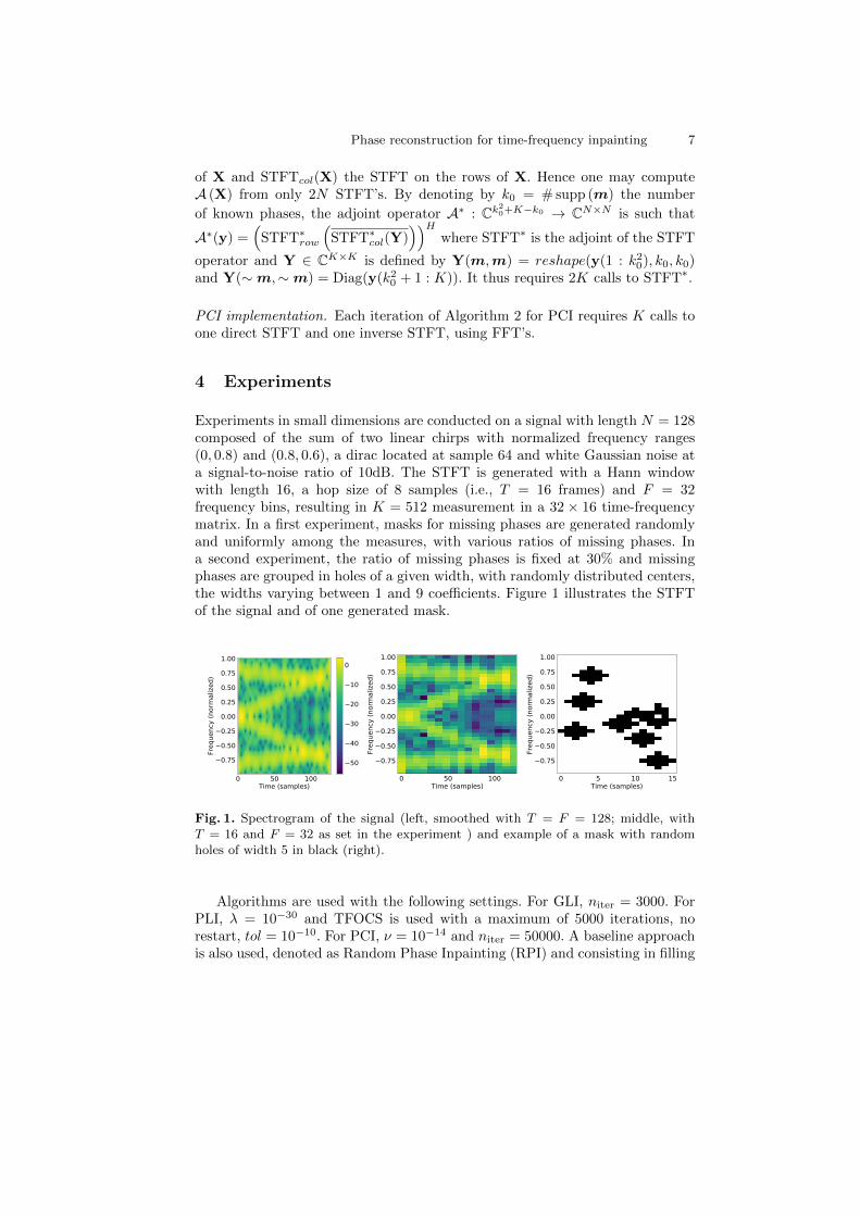
Experiments in small dimensions are conducted on a signal with length N = 128composed of the sum of two linear chirps with normalized frequency ranges(0, 0.8) and (0.8, 0.6), a dirac located at sample 64 and white Gaussian noise ata signal-to-noise ratio of 10dB. The STFT is generated with a Hann windowwith length 16, a hop size of 8 samples (i.e., T = 16 frames) and F = 32frequency bins, resulting in K = 512 measurement in a 32 × 16 time-frequencymatrix. In a first experiment, masks for missing phases are generated randomlyand uniformly among the measures, with various ratios of missing phases. Ina second experiment, the ratio of missing phases is fixed at 30% and missingphases are grouped in holes of a given width, with randomly distributed centers,the widths varying between 1 and 9 coefficients. Figure 1 illustrates the STFTof the signal and of one generated mask.

0 50 100Time (samples)

0.75

0.50

0.25

0.00

0.25

0.50

0.75

1.00

Freq

uenc

y (n

orm

alize

d)

50

40

30

20

10

0

0 50 100Time (samples)

0.75

0.50

0.25

0.00

0.25

0.50

0.75

1.00

Freq

uenc

y (n

orm

alize

d)

0 5 10 15Time (samples)

0.75

0.50

0.25

0.00

0.25

0.50

0.75

1.00

Freq

uenc

y (n

orm

alize

d)

Fig. 1. Spectrogram of the signal (left, smoothed with T = F = 128; middle, withT = 16 and F = 32 as set in the experiment ) and example of a mask with randomholes of width 5 in black (right).

Algorithms are used with the following settings. For GLI, niter = 3000. ForPLI, λ = 10−30 and TFOCS is used with a maximum of 5000 iterations, norestart, tol = 10−10. For PCI, ν = 10−14 and niter = 50000. A baseline approachis also used, denoted as Random Phase Inpainting (RPI) and consisting in filling


the missing phases by drawing random values independently and uniformely in[0, 2π[.

Performance is assessed in terms of relative reconstruction error up to a global

phase shift, defined by EdB(x, x) = 20 log10 minθ‖x−eıθx‖2‖x‖2 where x denotes the

original signal and x the reconstructed one.

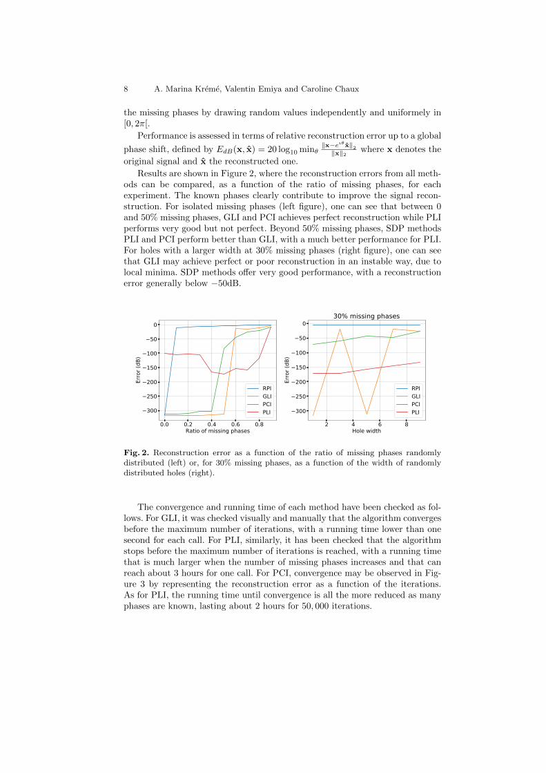
Results are shown in Figure 2, where the reconstruction errors from all meth-ods can be compared, as a function of the ratio of missing phases, for eachexperiment. The known phases clearly contribute to improve the signal recon-struction. For isolated missing phases (left figure), one can see that between 0and 50% missing phases, GLI and PCI achieves perfect reconstruction while PLIperforms very good but not perfect. Beyond 50% missing phases, SDP methodsPLI and PCI perform better than GLI, with a much better performance for PLI.For holes with a larger width at 30% missing phases (right figure), one can seethat GLI may achieve perfect or poor reconstruction in an instable way, due tolocal minima. SDP methods offer very good performance, with a reconstructionerror generally below −50dB.

0.0 0.2 0.4 0.6 0.8Ratio of missing phases

300

250

200

150

100

50

0

Erro

r (dB

)

RPIGLIPCIPLI

2 4 6 8Hole width

300

250

200

150

100

50

0

Erro

r (dB

)

30% missing phases

RPIGLIPCIPLI

Fig. 2. Reconstruction error as a function of the ratio of missing phases randomlydistributed (left) or, for 30% missing phases, as a function of the width of randomlydistributed holes (right).

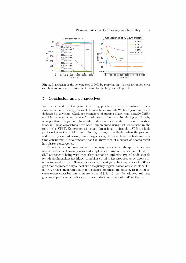
The convergence and running time of each method have been checked as fol-lows. For GLI, it was checked visually and manually that the algorithm convergesbefore the maximum number of iterations, with a running time lower than onesecond for each call. For PLI, similarly, it has been checked that the algorithmstops before the maximum number of iterations is reached, with a running timethat is much larger when the number of missing phases increases and that canreach about 3 hours for one call. For PCI, convergence may be observed in Fig-ure 3 by representing the reconstruction error as a function of the iterations.As for PLI, the running time until convergence is all the more reduced as manyphases are known, lasting about 2 hours for 50, 000 iterations.


0 10000 20000 30000 40000 50000Iterations

300

250

200

150

100

50

0

Erro

r (dB

)

Convergence of PCI

0% missing10% missing20% missing30% missing40% missing50% missing60% missing70% missing80% missing90% missing

0 10000 20000 30000 40000 50000Iterations

70

60

50

40

30

20

10

0

Erro

r (dB

)

Convergence of PCI, 30% missingwidth: 1width: 3width: 5width: 7width: 9

Fig. 3. Illustration of the convergence of PCI by representing the reconstruction erroras a function of the iterations in the same two settings as in Figure 2.

5 Conclusion and perspectives

We have considered the phase inpainting problem in which a subset of mea-surements have missing phases that must be recovered. We have proposed threededicated algorithms, which are extensions of existing algorithms, namely Griffinand Lim, PhaseLift and PhaseCut, adapted to the phase inpainting problem byincorporating the partial phase information as constraints in the optimizationprocess. Those algorithms have been implemented using fast transforms in thecase of the STFT. Experiments in small dimensions confirm that SDP methodsperform better than Griffin and Lim algorithm, in particular when the problemis difficult (more unknown phases, larger holes). Even if those methods are verytime consuming, it also appears that the knowledge of a subset of phases resultin a faster convergence.

Experiments may be extended to the noisy case where only approximate val-ues are available known phases and amplitudes. Time and space complexity ofSDP approaches being very large, they cannot be applied to typical audio signalsfor which dimensions are higher than those used in the proposed experiments. Inorder to benefit from SDP results, one may investigate the adaptation of SDP al-gorithms to process only a local time-frequency region instead of the whole STFTmatrix. Other algorithms may be designed for phase inpainting. In particular,some recent contributions to phase retrieval [12,4,13] may be adapted and maygive good performance without the computational limits of SDP methods.


References

1. S. Becker, E.J. Candes, and M. Grant. Templates for convex cone problems withapplications to sparse signal recovery. Technical report, Department of Statistics,Stanford University, 2010.

2. T. Bendory, Y. C. Eldar, and N. Boumal. Non-convex phase retrieval from STFTmeasurements. IEEE Transactions on Information Theory, 64(1):467–484, jan2018.

3. E. J Candes, Y. Eldar, T. Strohmer, and V. Voroninski. Phase retrieval via matrixcompletion. SIAM Rev, 57(2):225251, Nov 2015.

4. E. J. Candes, X. Li, and M. Soltanolkotabi. Phase retrieval via wirtinger flow:Theory and algorithms. IEEE Transactions on Information Theory, 61(4):1985–2007, apr 2015.

5. J.R. Fienup. Reconstruction of an object from the modulus. In Opt. Lett, volume 3,page 2729, 1978.

6. J.R. Fienup. Phase retrieval algorithms : a comparison. Applied Optics,21(15):27582769, 1982.

7. R.W Gerchberg and W. Saxton. A practical algorithm for the determination ofphase from image and diffraction plane pictures. Optik, 35:237246, 1972.

8. D. Griffin and Jae Lim. Signal estimation from modified short-time Fourier trans-form. IEEE Trans on Acoustics, Speech, Sig. Proc., 32(2):236–243, April 1984.

9. R. Hamon, V. Emiya, and C. Fvotte. Convex nonnegative matrix factorizationwith missing data. In Proc. IEEE International Workshop on Machine Learningfor Signal Processing (MLSP), 2016.

10. K. Jaganathan, Y. C. Eldar, and B. Hassibi. STFT phase retrieval: Uniquenessguarantees and recovery algorithms. IEEE Journal of Selected Topics in SignalProcessing, 10(4):770–781, jun 2016.

11. J. Le Roux, H. Kameoka, N. Ono, A. de Cheveigne, and S. Sagayama. Computa-tional auditory induction as a missing-data model-fitting problem with bregmandivergence. Speech Communication, In Press, 2010.

12. P. Netrapalli, P. Jain, and S. Sanghavi. Phase retrieval using alternating mini-mization. In in Adv. Neural Inf. Process. Syst., pages 2796–2804, 2013.

13. Z. Prusa, P. Balazs, and P. Sondergaard. A non-iterative method for reconstructionof phase from stft magnitude. In IEEE/ACM Transactions on Audio, Speech, andLanguage Processing, volume 25, pages 1154–1164, 2017.

14. P. Smaragdis, B. Raj, and M. Shashanka. Missing data imputation for spectralaudio signals. In Proc. of MLSP, Grenoble, France, September 2009.

15. I. Waldspurger, A. dAspremont, and S. Mallat. Phase recovery, maxcut and com-plex semidefinite programming. Math. Prog, 149(1-2):47–81, Feb. 2015.

16. Z. Wen, D. Goldfarb, and K. Scheinberg. Block coordinate descent methods forsemidefinite programming. In Handbook on Semidefinite, Conic and PolynomialOptimization, springer edition, 2012.

phase reconstruction for time-frequency inpainting

Documents