U.S. Department of the InteriorU.S. Geological SurveyU.S. Department of the InteriorU.S. Geological Survey

Petroleum System Modeling Capabilitiesfor Use in Oil and Gas Resource AssessmentsPetroleum System Modeling Capabilitiesfor Use in Oil and Gas Resource Assessments

Open-File Report 2006–1024Open-File Report 2006–1024

Present-day catchments on the Upper Cretaceous Viking N

Petroleum System Modeling Capabilities for Use in Oil and Gas Resource Assessments

By Debra K. Higley, Michael Lewan, Laura N.R. Roberts, and Mitchell E. Henry

Open-File Report 2006–1024

U.S. Department of the InteriorU.S. Geological Survey

U.S. Department of the InteriorGale A. Norton, Secretary

U.S. Geological SurveyP. Patrick Leahy, Acting Director

U.S. Geological Survey, Reston, Virginia: 2006

Posted online March 2006 Version 1.0

This publication is only available online at http://www.usgs.gov/of/2006/1024/

For more information on the USGS--the Federal source for science about the Earth, its natural and living resources, natural hazards, and the environment: World Wide Web: http://www.usgs.gov Telephone: 1-888-ASK-USGS

Any use of trade, product, or firm names is for descriptive purposes only and does not imply endorsement by the U.S. Government.

Although this report is in the public domain, permission must be secured from the individual copyright owners to reproduce any copyrighted materials contained within this report.

Suggested citation:Debra K. Higley, Michael Lewan, Laura N.R. Roberts, and Mitchell E. Henry, 2006, Petroleum System Modeling Capabilities for Use in Oil and Gas Resource Assessments: U.S. Geological Survey Open-File Report 2006-1024

iii

Contents

Executive Summary .......................................................................................................................................1Introduction.....................................................................................................................................................2Computer Requirements ...............................................................................................................................31-D Modeling ..................................................................................................................................................4

Background............................................................................................................................................4Recommended Data .............................................................................................................................4Time, Equipment, and Personnel Requirements ..............................................................................5Advantages of Using 1-D Models ......................................................................................................5Limitations of 1-D Modeling ................................................................................................................5

2-D Modeling ..................................................................................................................................................9Background............................................................................................................................................9Recommended Data .............................................................................................................................9Time and Personnel Requirements ....................................................................................................9Advantages of Using 2-D Models ......................................................................................................9Limitations of 2-D Modeling ..............................................................................................................10

3-D Modeling ................................................................................................................................................11Background..........................................................................................................................................11Requirements for 3-D Modeling .......................................................................................................11Time and Personnel Requirements ..................................................................................................15Advantages of 3-D Models ................................................................................................................15Requirements and Limitations of 3-D Modeling ............................................................................16

Conclusions...................................................................................................................................................17Acknowledgements .....................................................................................................................................17References ....................................................................................................................................................17

Figures 1. Example of a template used for input to the PetroMod® one-dimensional

modeling program .........................................................................................................................6 2. Events chart showing petroleum systems elements of the Lower

Cretaceous Mannville Formation, Western Canada Sedimentary Basin ............................7 3. Plots showing burial history of the Tomahawk 16-18 well, northern Alberta .....................8 4. Map showing two-dimensional flowpaths and accumulations of oil and gas

in the Lower Cretaceous Mannville Group .............................................................................10 5. Block diagram with a front-facing east-west cross section that depicts all

geologic intervals used in the three-dimensional model across northern Alberta .........12 6. Map view of early generation and emplacement of hydrocarbons into the

Lower Cretaceous Mannville Group to form tar sands ........................................................13 7. Three-dimensional diagram showing Jurassic Nordegg Member source rocks ............14

Executive Summary

Petroleum resource assessments are among the most highly visible and frequently cited scientific products of the U.S. Geo-logical Survey. The assessments integrate diverse and extensive information on the geologic, geochemical, and petroleum pro-duction histories of provinces and regions of the United States and the World. Petroleum systems modeling incorporates these geoscience data in ways that strengthen the assessment process and results are presented visually and numerically. The purpose of this report is to outline the requirements, advantages, and lim-itations of one-dimensional (1-D), two-dimensional (2-D), and three-dimensional (3-D) petroleum systems modeling that can be applied to the assessment of oil and gas resources. Primary focus is on the application of the Integrated Exploration Sys-tems (IES) PetroMod® software because of familiarity with that program as well as the emphasis by the USGS Energy Program on standardizing to one modeling application. The Western Canada Sedimentary Basin (WCSB) is used to demonstrate the use of the PetroMod® software.

Petroleum systems modeling quantitatively extends the “total petroleum systems” (TPS) concept (Magoon and Dow, 1994; Magoon and Schmoker, 2000) that is employed in USGS resource assessments. Modeling allows integration of state-of-the-art analysis techniques, and provides the means to test and refine understanding of oil and gas generation, migration, and accumulation. Results of modeling are pre-sented visually, numerically, and statistically, which enhances interpretation of the processes that affect TPSs through time. Modeling also provides a framework for the input and process-ing of many kinds of data essential in resource assessment, including (1) petroleum system elements such as reservoir, seal, and source rock intervals; (2) timing of depositional, hiatus, and erosional events and their influences on petroleum systems; (3) incorporation of vertical and lateral distribution and lithologies of strata that compose the petroleum systems; and (4) calculations of pressure-volume-temperature (PVT) histories. As digital data on petroleum systems continue to expand, the models can integrate these data into USGS resource assessments by building and displaying, through time, areas of petroleum generation, migration pathways, accumulations, and relative contributions of source rocks to the hydrocarbon components.

IES PetroMod® 1-D, 2-D, and 3-D models are integrated such that each uses the same variables for petroleum systems modeling. 1-D burial history models are point locations, mainly wells. Maps and cross-sections model geologic information in two dimensions and can incorporate direct input of 2-D seismic data and interpretations using various formats. Both 1-D and 2-D models use data essential for assessments and, following data compilation, they can be completed in hours and retested in minutes. Such models should be built early in the geologic assessment process, inasmuch as they incorporate the petroleum system elements of reservoir, source, and seal rock intervals with associated lithologies and depositional and ero-sional ages. The models can be used to delineate the petroleum systems. A number of 1-D and 2-D models can be constructed across a geologic province and used by the assessment geolo-gists as a 3-D framework of processes that control petroleum generation, migration, and accumulation. The primary limita-tion of these models is that they only represent generation, migration, and accumulation in two dimensions.

3-D models are generally built at reservoir to basin scales. They provide a much more detailed and realistic representa-tion of petroleum systems than 1-D or 2-D models because they portray more fully the temporal and physical relations among (1) burial history; (2) lithologies and associated changes through burial in porosity, permeability, and compaction; (3) hydrodynamic effects; and (4) other parameters that influence petroleum generation, migration, and accumulation. Consider-ably more time, data, and computer resources are required than for 1-D or 2-D models. These factors are dependent upon data quality and quantity, and the size and complexity of the model. 3-D models are built using structural and isopach surfaces that are selected based on criteria such as chronostratigraphic divi-sions, petroleum system boundaries, major tectonic events that influenced thermal history, or other criteria, with the data being derived from sources that include well databases, maps, and (or) cross sections. Upon completion of a 3-D model, geosci-entists can apply the results to refining petroleum systems, evaluating timing of oil and (or) gas generation, migration, and accumulation relative to trap formation, and other factors important to resource assessments. Modifications of models can generally be done in minutes; however, rerunning the models with new parameters may take hours to days depending upon complexity and the computer platform(s) used.

Petroleum System Modeling Capabilities for Use in Oil and Gas Resource Assessments

By Debra K. Higley, Michael Lewan, Laura N.R. Roberts, and Mitchell E. Henry

Although not required, 1-D, 2-D, and 3-D models can be externally calibrated using information from maps and cross sections, vitrinite reflectance (R

o) and other thermal matura-

tion data, and temperature and pressure data. Various default and user-defined kinetic algorithms can be assigned to source rock intervals to model primary oil and gas generation and secondary oil cracking. Normal and wrench faults can be open or closed for variable time periods. High-angle reverse faults, as along the eastern boundary of the Canadian Rockies in the WCSB, can be incorporated as a series of vertical faults that are horizontally connected across layer boundaries. Vari-able permeability, including shale-gouge properties, can be assigned to the fault systems to model the effects on hydrocar-bon migration.

Following is a list of some variables integrated through time, as well as results from 3-D petroleum systems models and to a lesser extent 1-D and 2-D models. Many of these parameters can be risked using the IES PetroRisk® module. PetroRisk enables users to define boundaries and distributions of variables such as thickness and organic-matter richness of source rock, reservoir and trap geometry, porosity, perme-ability, seal integrity, and timing of oil and gas generation and migration. These distributions are then sampled using Monte Carlo, Latin Hypercube, and other methods, and multiple pro-cessing runs then enable statistical evaluations and correlations of the results to be made in order to assess the effects of the uncertainties of the data on the results of the modeling. Results then include some of the following:

1. Timing and extent of thermal maturation for each source rock interval. The 3-D model displays this information as map images, cross sections, or as point sources through 1-D extractions.

2. Migration flowpaths and vectors in 2-D or 3-D space, which show time increments of generation, directions of flow, and accumulations of oil and gas.

3. Percent contributions and volumes of generated hydrocarbons through time for each source rock unit. Results are tabulated and displayed at scales ranging from single accumulations to the entire model.

4. Percent transformation of kerogen in source rocks to oil and (or) gas. The extent of kerogen transformation is a record of the petroleum generation history that is displayed visually and in tabular form.

5. Coal rank through time can be evaluated using Swee-ney and Burnham (1990) Easy%R

o, adsorption mass,

and other modeled calculations. Results could be used to assess coal and coalbed methane resources; amount of adsorbed methane commonly increases with coal rank.

6. PVT calculations for all intervals, including capillary, lithologic, and hydrodynamic pressure. These values can be used to predict the formation volume factor

(FVF) for oil and gas, and possibly fluid composition, gas-oil ratios, condensate occurrences, and pres-sure history. Hydrocarbon composition and volumes are calculated by PetroMod® for both surface and subsurface conditions. This information is useful for assessing conventional as well as unconventional resources.

7. Compaction history using default values assigned by PetroMod® or user-defined porosity/permeability/depth through time can be used for the lithologies. Analogs can be applied for this and numerous other parameters in the modeling.

8. Catchments are structural segmentation of layers in a model that are primarily used to show oil and gas migration pathways, spillpoints, and accumulations across these surfaces.

9. Timing of hydrocarbon generation relative to trap formation. Also, effects on hydrocarbon migration of events such as faulting, basin uplift and tilting, salt movement, and intrusions.

Introduction

The methodology used by the U.S. Geological Survey (USGS) in assessing undiscovered conventional and uncon-ventional hydrocarbon resources evolves with increased understanding of controls on petroleum generation, migration, accumulation, and production. One-dimensional (1-D), two-dimensional (2-D), and three-dimensional (3-D) petroleum systems modeling are tools for the assessments. The modeling and the assessments both apply the petroleum systems concept (Magoon and Dow, 1994; Magoon and Schmoker, 2000) to vertically and laterally divide provinces into mappable volumes of rocks that share a common history of genera-tion, migration, and accumulation of petroleum. Much of this information is analyzed by USGS geoscientists by integrating data at well-to-basin scales, review of publications on these and similar areas, and use of analogs for strata in frontier areas. USGS assessments are increasingly data intensive; it is therefore important to integrate these data in ways that best show the interconnection of petroleum system processes, with results that can be presented to a broad audience. These models allow geoscientists to evaluate the consistency of their interpreted and the simulated basin history.

Use of PetroMod® in USGS assessments is being evalu-ated in this report because it is currently being used in research studies of the Western Canada Sedimentary Basin (WCSB), as well as in resource assessments of provinces worldwide. Petro-leum systems modeling software is used to reconstruct the geologic history at point, reservoir, and basin scales. Modeling uses the following data that contribute to assessment of oil and gas resources:

� Petroleum System Modeling

1. Locations, depths, and areal distribution of all strata can be derived from a number of sources that include well logs, databases, published maps and cross sec-tions, and seismic surveys.

2. Ages and lithologies for all formation intervals within the study area. A spreadsheet that contains these data, time periods of erosion and tectonic events, and associated references is useful for sub-sequent grouping of these formations into intervals for the petroleum systems model. The modeling process does not require grouping of strata into petroleum systems or determination of petroleum system boundaries, although it is helpful to compare the expected boundaries to those interpreted from the modeling results.

3. In order to apply results of the modeling to relative contributions through time of source rock intervals to generated, migrated, and accumulated oil and (or) gas, required input data for source rocks includes kerogen types, total organic carbon (TOC), hydrocar-bon indices (HI), and kinetic algorithms. It is best to have results of pyrolysis analyses on immature source rocks in each modeled province or area; however, analogs can be also used for these variables.

4. Time periods and areas of nondeposition, uplift, and erosion. Eroded thicknesses can be estimated using 1-D and 2-D models, and 1-D extractions from the 3-D model.

5. Vertical and lateral extent of faults, timing of onset of faulting, and assignment of whether faults or seg-ments of faults are open or closed.

6. Surface and subsurface temperatures through time, including heat flow history. These values can also be generated using PetroMod®, but it is useful to have external sources of data to document and calibrate the 1-D, 2-D, and 3-D models.

7. Water depth through time.

8. These data are useful for external calibration of the models: corrected borehole or drillstem test tempera-tures, and vitrinite reflectance (R

o), time-temperature

indices, fission track, or other thermal maturation data.

Reservoir- to province-scale regions are divided on the 2-D map and 3-D models into catchments; these are structur-ally-determined outlines of areas for oil and gas migration and accumulation. The accuracy of the area of each catch-ment depends partly on the grid spacing of the layers in a model, which can be changed by the user. Finer spaced grids in the generated model result in more detailed division of the catchments. Catchments in the Illinois Basin were mapped using an inverted hydrologic-flow algorithm using ESRI

Arc® software (Lewan and others, 2002; Higley and others, 2003). Use of the catchments can assist resource assessment by illustrating potential areas for hydrocarbon accumulation, based on whether (and when) oil and gas migrated through or were trapped within them. Maps and cross section models can incorporate 2-D flow of fluids. PetroMod® software, for example, models vertical and (or) lateral flow through strata and along faults and other surfaces. Vertical and lat-eral changes in lithology and associated physical properties can be assigned to geologic intervals, or layers, within the models.

PetroMod® has functions for generating, editing, and gridding maps and model intervals. These operations were conducted outside PetroMod® using ESRI® Arc® software or geologic mapping software, such as Dynamic Graphics® EarthVision®. (Note: Dynamic Graphics and Earthvision® are registered trademarks of Dynamic Graphics, Inc.) Because these maps and associated data were used for other assess-ment purposes, as well as for building a 3-D geologic model, it was more efficient to generate and edit the layers for 2-D and 3-D petroleum systems models outside of PetroMod®. The resulting grids or the 3-D geologic Earthvision® model are then imported directly into the PetroMod® models. Pet-roMod® also has modules that allow for direct import of 2-D seismic data and interpretations, and allows for a number of seismic data formats. Grids need to be exported from Earthvi-sion® in zmap format to be read using PetroMod®. Zmap is an ASCII file format that contains a header record, and grid node values in rows and columns

Modifying and rerunning 1-D and 2-D models can be accomplished in minutes. It is also relatively easy to modify 3-D model parameters, but considerable computer time is needed to run full 3-D models. This time can be minimized by selecting small areas of the model for separate runs, often individual catchment areas, which is useful for evaluating effects of the modifications. Deactivation of 2-D and 3-D hydrocarbon generation and migration results in a faster run-time for the 3-D model, which is useful for calibrating geologic and tectonic events and surfaces.

Computer Requirements

IES software is supported on Windows XP®, Linux®, and UNIX® operating systems on PC, Silicon Graphics Incorporated® (SGI), and Sun® computer platforms. The user interface and data formats are the same for all platforms. Relatively small amounts of disk space and computer time are needed to generate 1-D or 2-D models, which can be run on any of the computer platforms. Generation of 3-D models, on the other hand, requires considerable memory, processing time, and storage space; a petroleum systems model at a province scale is preferably generated using a Linux cluster of linked PCs because of the shorter comput-ing and display time provided by multiple processors. The

Computer Requirements �

Sun and SGI platforms can also be used to run 3-D models, but long processing time and memory limitations may require the model to be simulated at lower resolution. The 3-D model of Iraq was simulated using one processor on a Sun Solaris computer (Pitman and others, 2003); the province was divided into 5 models so that 1-km grid spacing could be used. Computing capabilities may not be adequate to process or view the full 3-D PetroMod® models at very fine grid spacing. Options are multi-1-D processing for genera-tion potential calculations, or full-scale models with coarser grids, such as 15-km spacing; smaller areas of interest can then be modeled by creating subsets within the province and saving them as new models. The advantages of the smaller area are faster modification and processing time, better grid resolution, the ability to use full 3-D processing, and (or) being better able to examine areas of interest within the large model.

An additional cost of using the linked PCs and of the second parallel processor on the Sun and SGI systems is that IES requires additional parallel processor licenses for each additional processor. One issue with the use of multiple pro-cessors is additional maintenance by computer support. Also required are computer support personnel proficient in Linux or UNIX (Sun, SGI) systems and resolving software/hardware problems. Software upgrades and bug fixes are commonly available for download at the IES website.

1-D Modeling

Background

The primary purpose of 1-D, or burial history, models is to reconstruct the geologic history at one or more points in a region. The modeling should be incorporated into assessments of oil and gas resources. Essentially all of the information needed for 1-D burial history modeling is also required in the assessment process, and building 1-D models requires scien-tists to refine the stratigraphy within the province and to assign lithologies and age ranges to those intervals important in the assessments. Because burial history models are used to define petroleum systems, it is not necessary to first assign petroleum system elements and boundaries. Assignment of strata to over-burden, seal, reservoir, and source intervals, however, is useful for a PetroMod®-generated total petroleum systems events chart and to tie the models to the assessments.

The assessment of the Southwestern Wyoming Province (Roberts and others, 2004) is a good example of the use of 1-D modeling. The models resulted in dating peak oil and gas gen-eration and the times of generation for a series of source rocks in the province. Temperature histories, R

o data, and deposition

and erosional histories were integrated into a series of burial history plots and diagrams that illustrate the relative effects of these factors on hydrocarbon generation at individual points across the province.

Recommended Data

1. Names of formation intervals. Examples are the name of the primary formation or stratigraphic interval within that layer, or assigned codes.

2. Well name and latitude-longitude or other map coordinate location. If the 1-D burial history models are used to calibrate 2-D or 3-D PetroMod® models, then all location data should use the same coordinate system and parameters.

3. Data sources for formation tops, and well and field name and locations include:

a. Publications, cross sections, seismic sections, outcrop descriptions.

b. Core descriptions, well logs.

c. State records of drilled water or oil and gas wells.

d. Commercial databases, such as IHS Energy Well History Control (U.S.), Accumap (Canada), and Petroconsultants well and field databases.

4. Strata depth or elevation relative to sea level. Units are meters or feet. Stratigraphic intervals should be subdivided if they are very thick and (or) were depos-ited over a long period of time, especially when there are numerous R

o and other thermal maturity data.

They are best divided if the interval is very hetero-geneous— for example, the upper portion is seal, the middle is reservoir, and the lower is the hydrocar-bon source, or the lithologic variation is significant enough to influence model results.

5. Ages of intervals in millions of years before present (Ma). Intervals within PetroMod® models can be assigned based on chronostratigraphic, lithostrati-graphic, major tectonic events, and other criteria.

6. Time periods (ages in terms of Ma) of nondeposition or erosion. Estimates of the thickness and lithology of eroded sections are useful for comparison to those determined using the modeling.

7. Paleowater depth, heat flow, and surface temperature through time. Options include using default or user-defined values for these parameters. PetroMod can also calculate surface temperature through time.

8. Corrected borehole/drillstem test (DST) temperature and R

o can be used for external calibration of the

models, although it is not required to run the models. TOC and HI data are needed for source rock intervals if kinetic algorithms are used to model primary and secondary generation of oil and gas.

� Petroleum System Modeling

Time, Equipment, and Personnel Requirements

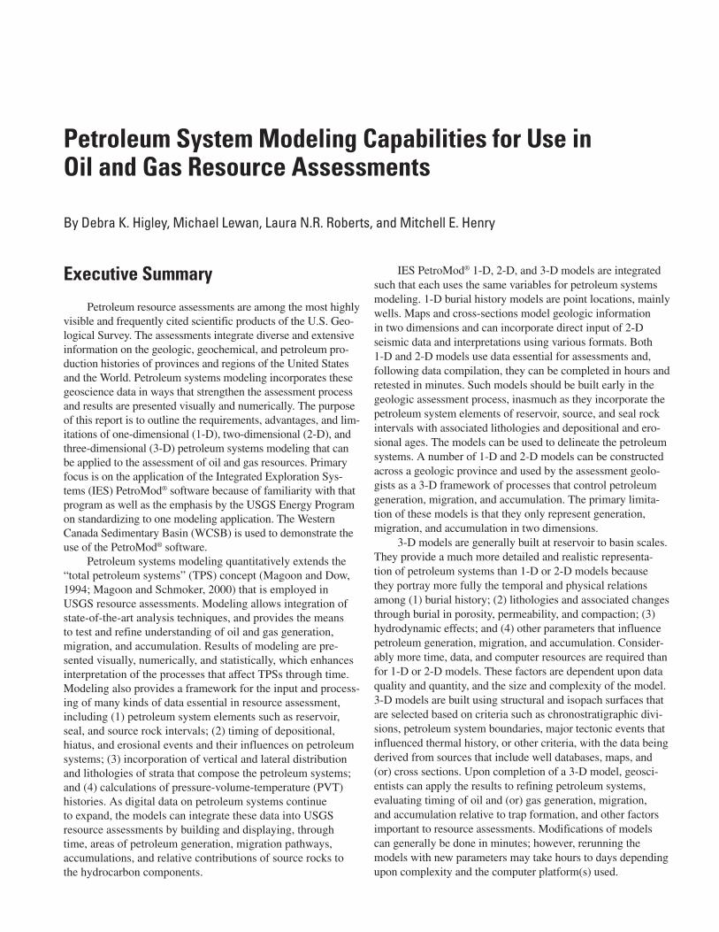
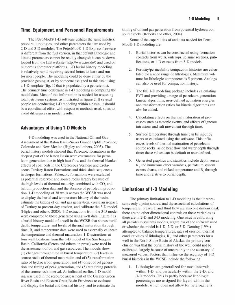
The PetroMod® 1-D software utilizes the same kinetics, pressure, lithologies, and other parameters that are used by 2-D and 3-D modules. The PetroMod® 1-D Express freeware is different from the full version, in that default lithologic and kinetic parameters cannot be readily changed; it can be down-loaded from the IES website (http://www.ies.de/) and used on numerous computer platforms. 1-D burial history modeling is relatively rapid, requiring several hours to learn and run for most people. The modeling could be done either by the province geologist, or by someone assigned to this task using a 1-D template (fig. 1) that is populated by a geoscientist. The primary time constraint in 1-D modeling is compiling the model data. Most of this information is needed for assessing total petroleum systems, as illustrated in figure 2. If several people are conducting 1-D modeling within a basin, it should be a coordinated effort with respect to methods used, so as to avoid differences in model results.

Advantages of Using 1-D Models

1-D modeling was used in the National Oil and Gas Assessment of the Raton Basin-Sierra Grande Uplift Province, Colorado and New Mexico (Higley and others, 2005). The burial history models showed that Paleozoic formations in the deepest part of the Raton Basin were overmature for petro-leum generation due to high heat flow and the thermal-blanket effects of coal beds in the Cretaceous Vermejo and Creta-ceous-Tertiary Raton Formations and thick shale sequences in deeper formations. Paleozoic formations were excluded as potential reservoir and source rocks largely because of the high levels of thermal maturity, combined with CO

2 and

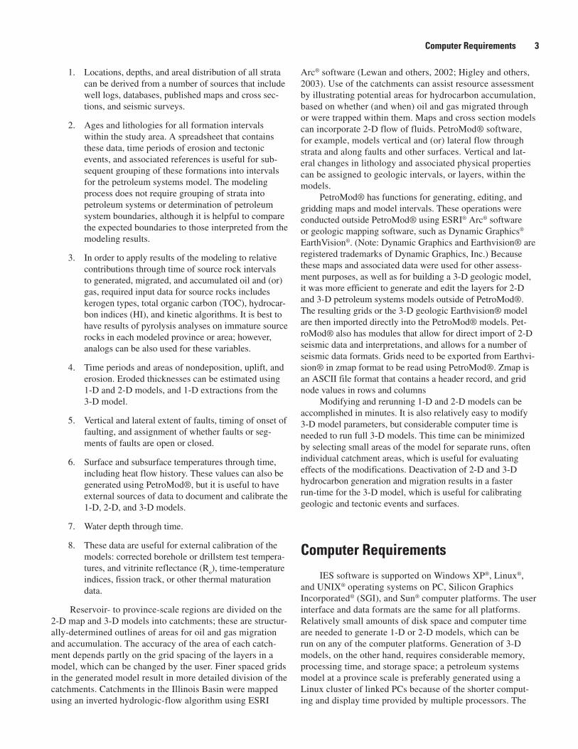
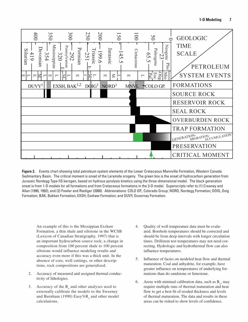
helium production data and the absence of petroleum produc-tion. 1-D modeling of 38 wells across the WCSB was used to display the burial and temperature history of the basin, estimate the timing of oil and gas generation, create an isopach of Tertiary to present-day erosion, and calibrate the 3-D model (Higley and others, 2005); 1-D extractions from the 3-D model were compared to those generated using well data. Figure 3 is a burial history model of a well in the WCSB that shows burial depth, temperature, and levels of thermal maturation through time; R

o and temperature data were used to externally calibrate

the temperature and thermal maturation. 1-D extractions at four well locations from the 3-D model of the San Joaquin Basin, California (Peters and others, in press) were used in the assessment of oil and gas resources. The models show (1) changes through time in burial temperature; (2) levels in source rocks of thermal maturation and of (3) transformation ratio of hydrocarbon generation; and (4) onset of oil genera-tion and timing of peak generation, and (5) remaining potential of the source rock interval. As indicated earlier, 1-D model-ing was used in the resource assessment of the Greater Green River Basin and Eastern Great Basin Provinces to evaluate and display the burial and thermal history, and to estimate the

timing of oil and gas generation from potential hydrocarbon source rocks (Roberts and other, 2004).

Some of the capabilities of and data needed for Petro-Mod® 1-D modeling are:

1. Burial histories can be constructed using formation contacts from wells, outcrops, seismic sections, pub-lications, or 1-D extracts from 3-D models.

2. Porosity/permeability compaction histories are calcu-lated for a wide range of lithologies. Minimum vol-ume for lithologic components is 5 percent. Analogs can also be used for compaction history.

3. The full 1-D modeling package includes calculating PVT and providing a range of petroleum generation kinetic algorithms; user-defined activation energies and transformation ratios for kinetic algorithms can also be added.

4. Calculating effects on thermal maturation of pro-cesses such as tectonic events, and effects of igneous intrusions and salt movement through time.

5. Surface temperature through time can be input by users or calculated using the software. This influ-ences levels of thermal maturation of petroleum source rocks, as do heat flow and water depth through time; these values can be default or user defined.

6. Generated graphics and statistics include depth versus R

o and numerous other variables, petroleum system

events charts, and risked temperature and Ro through

time and relative to burial depth.

Limitations of 1-D Modeling

The primary limitation to 1-D modeling is that it repre-sents only a point source, and the associated calculations of temperature, pressure, and fluid flow are also one dimensional; there are no other dimensional controls on these variables as there are in 2-D and 3-D modeling. One issue is calibrating all petroleum systems models, regardless of the software used or whether the model is 1-D, 2-D, or 3-D. Deming (1994) attempted to balance temperatures, rates of erosion, thermal conductivities of lithologies, R

o, and other parameters for a

well in the North Slope Basin of Alaska; the primary con-clusion was that the burial history of the well could not be calibrated, largely because of uncertainty in the accuracy of measured values. Factors that influence the accuracy of 1-D burial histories in the WCSB include the following:

1. Lithologies are generalized for most intervals within 1-D, and particularly within the 2-D, and 3-D models. This is partly because lithologic percentages are assigned for layers within the models, which does not allow for heterogeneity.

1-D Modeling �

Present Deposition Age Erosion Age PetroSysEssential

TOC

[wt%]

HI Petroleum PetroleumName Top Base Thickness

ErodedThickness from to from to Lithology Kinetics Kinetics

[meter] [meter] [meter] [meter] [Ma] [Ma] [Ma] [Ma] Elements [mg/g TOC]Water depth 0 0 0 0 0Quaternary 20 0 20 1.6 0 SAND&SHAL Overburden Rock 0 0 nonePaskapoo 300 20 280 1200 67 57.8 57.8 1.6 SHALE Overburden Rock 0 0 noneBattle 740 300 440 72 67 SHALE Overburden Rock 0 0 noneBearpaw 800 740 60 75 72 SHALE Source/Seal Rock 0 0 noneBelly River 1093 800 293 79 75 SAND&SHAL Source/Reservoir Rock 0 0 noneLea Park 1210 1093 117 84 79 SHALEsilt Seal Rock 0 0 noneU Colorado Gp 1539 1210 329 91 84 SHALEsilt Source Rock 0 0 noneSecond White Specks 1647 1539 108 96 91 SHALEsilt Source/Reservoir Rock 5.1 0 noneFish Scale Zone 1671 1647 24 97 96 SHALE Source/Seal Rock 3.2 0 noneL Viking 1744 1671 73 104 97 SAND&SHAL Reservoir Rock 0 0 noneBlairmore 1925 1744 181 119 104 SHALE Source/Seal Rock 0 0 noneJurassic-Miss 1925 1925 0 340 150 LIMEshaly Overburden Rock 0 0 nonePekisko 1992 1925 67

400345 340

150 119LIMESTONE Reservoir Rock 0 0 none

Banff 2145 1992 153 357 345 SHALE Source/Reservoir Rock 2 0 noneExshaw 2148 2145 3 363 357 SHALE Source/Seal Rock 0 0 noneWabamun 2348 2148 200 366 363 SHALEsilt Source/Reservoir Rock 0 0 noneCalmar 2349 2348 1 367.5 366 SHALE Source/Seal Rock 0 0 noneNisku 2395 2349 46 369 367.5 LIMEshaly Source/Reservoir Rock 0 0 noneIreton 2515 2395 120 371 369 SHALE Reservoir Rock 2.5 0 noneDuvernay 2600 2515 85 372 371 LIMEshaly Source/Seal Rock 0 0 noneCooking Lake 2700 2600 100 373 372 LIMESTONE Underburden Rock 0 0 noneBeaverhill Lake 2850 2700 150 377 373 LIMEshaly Source/Reservoir Rock 0 0 noneElk Point Gp 2900 2850 50 407 377 LIMEshaly Seal Rock 0 0 noneBasal Ss 3500 2900 600 570 407 SAND&SHAL Underburden Rock 0 0 none

3500

Age Water Depth Age SWI Age HF[Ma] [meter] [Ma] [celsius] [Ma] [mW/m2]

0 0 0 20 0 4070 10 70 22 40 40

100 40 100 23 80 40570 50 570 7 570 40

Figure 1. Example of a template used for input to the PetroMod® one-dimensional modeling program. Background grid shows parameters, such as formation or depth interval name, depths in meters (or feet), ages in years or millions of years (Ma), lithologies, total organic carbon (TOC) in percent or mg/g of TOC, hydrocarbon indices (HI) values, and name of petroleum kinetic algorithm. The yellow inset grid is a second template for the one-dimensional modeling that includes age ranges of surface water depth in meters or feet, surface temperature through time (SWI) in degrees Celsius (or Kelvin, Fahrenheit), and of heat flow (HF) in watts or milliwatts per square meter (mW/m2) or heat flow units. Surface temperature through time can be calculated using the PetroMod® program; water depth, heat flow, and other parameters are supplied by the user.

�

Petroleum System

Modeling

An example of this is the Missippian Exshaw Formation, a thin shale and siltstone in the WCSB (Lexicon of Canadian Stratigraphy, 1997) that is an important hydrocarbon source rock; a change in composition from 100 percent shale to 100 percent siltstone would influence modeling results and accuracy even more if this was a thick unit. In the absence of core, well cuttings, or other descrip-tions, rock compositions are generalized.

2. Accuracy of measured and assigned thermal conduc-tivity of lithologies.

3. Accuracy of the Ro and other analyses used to

externally calibrate the models to the Sweeney and Burnham (1990) Easy%R

o and other model

calculations.

4. Quality of well temperature data must be evalu-ated. Borehole temperatures should be corrected and should be from deep intervals with longer circulation times. Drillstem test temperatures may not need cor-recting. Hydrologic and hydrothermal flow can also influence temperatures.

5. Influence of facies on modeled heat flow and thermal maturation. Coal and anhydrite, for example, have greater influence on temperatures of underlying for-mations than do sandstone or limestone.

6. Areas with minimal calibration data, such as Ro, may

require multiple runs of thermal maturation and heat flow to get a best-fit of eroded thickness and levels of thermal maturation. The data and results in these areas can be risked to show levels of confidence.

0

100

200

300

400 50

150

250

350

Paleogene

Cretaceous

Jurassic

Triassic

Permian

65.5

145.5

199.6

251

354

419Silurian

Devonian

292

320

E E

E E

E EEEM M M ML L L L L L L L

Mississippian

Pennsylvanian

Neogene

23

PalEocO

ligM

ioPlio

PRESERVATIONCRITICAL MOMENT

GENERATION-TRAP FORMATIONOVERBURDEN ROCK

RESERVOIR ROCKSEAL ROCK

SOURCE ROCKFORMATIONS

PETROLEUMSYSTEM EVENTS

GEOLOGICTIMESCALE

ACCUMULATIONMIGRATION-

MNVL COLO GP.DUVY EXSH, BAK DOIG NORD1,21 11

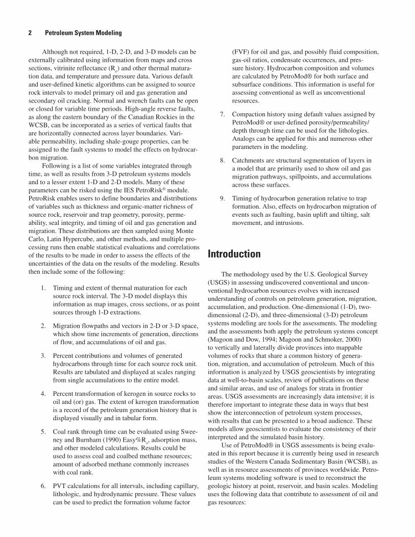
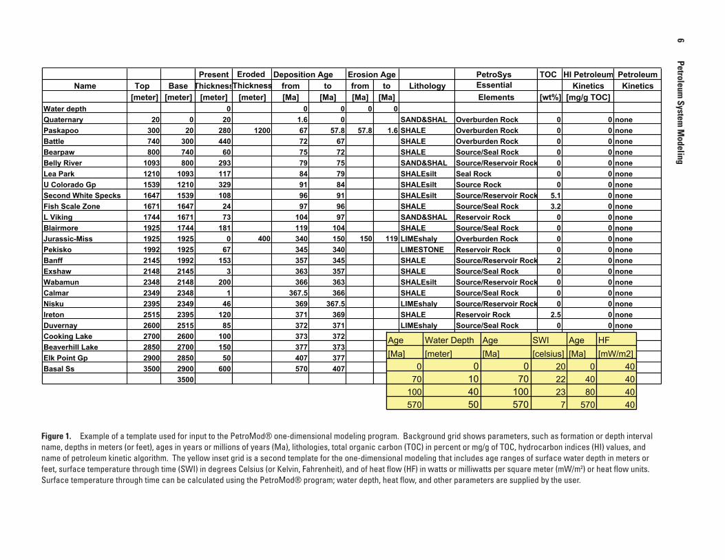
Figure �. Events chart showing total petroleum system elements of the Lower Cretaceous Mannville Formation, Western Canada Sedimentary Basin. The critical moment is onset of the Laramide orogeny. The green box is the onset of hydrocarbon generation from Jurassic Nordegg Type IIS kerogen, based on hydrous pyrolysis kinetics using the three-dimensional model. The black generation onset is from 1-D models for all formations and from Cretaceous formations in the 3-D model. Superscripts refer to (1) Creaney and Allan (1990, 1992), and (2) Fowler and Riediger (2000). Abbreviations: COLO GP., Colorado Group; NORD, Nordegg Formation; DOIG, Doig Formation; BAK, Bakken Formation; EXSH, Exshaw Formation; and DUVY, Duvernay Formation.

1-D Modeling �

Percent vitrinite reflectance

0.4 – 0.6 1.2 – 1.4

0.6 – 0.8 1.4 – 1.6

0.8 – 1.0 1.6 – 1.8

1.0 – 1.2 1.8 – 2.0

0

1,000

2,000

3,000

4,000

4,594

BU

RIA

L D

EPTH

, IN

MET

ERS

Temperature, in degrees Celsius

Sweeney and Burnham (1990) Easy%R %R

0

1,000

2,000

3,000

AGE, IN MILLIONS OF YEARS

0

1,000

2,000

3,000

DEP

TH, I

N M

ETER

S

0.10 1.00o

DEP

TH, I

N M

ETER

S

5 80

o

TR

500 400 300 200 100 0

Figure �. Plots showing burial history from Cambrian to Holocene time, based on strata penetrated in the Tomahawk 16-18 well, northern Alberta. Cretaceous and older formations are thermally mature for oil generation; onset of oil generation is about 75 million years ago (Ma) for Devonian Woodbend Group source rocks and about 65 Ma for Cretaceous Mannville Group source rocks. Colors are estimated percent vitrinite reflectance (Ro) of rocks based on modeling using the Sweeney and Burnham (1990) Easy%Ro kinetic algorithm. The red and blue dots on the upper left chart are Ro data from Stasiuk and Fowler, 2002, and Stasiuk and others (2002); these are an external calibration to the calculated curve. Green dots on the lower left chart are temperatures determined from drillstem test or corrected borehole temperatures; these are used to calibrate the temperature versus depth calculation that is based largely on lithology, heat flow, and depth of burial.

�

Petroleum System

Modeling

�-D Modeling

Background

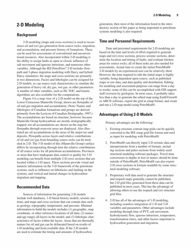
2-D modeling (maps and cross-sections) is used to recon-struct oil and (or) gas generation from source rocks, migration, and accumulation, and pressure history of formations. These can be used for assessments of conventional and unconven-tional resources. Also incorporated within 2-D modeling is the ability to assign faults as open or closed, influence of salt movement and igneous intrusions, and numerous other variables. Although the IES PetroFlow® 2-D includes flow-path and 3-phase migration modeling with Darcy and hybrid Darcy simulators, the maps and cross-sections are primarily in two dimensions. Facies and lithologies can be assigned for 2-D models, as can source rock characteristics to simulate the generation of heavy oil, dry gas, wet gas, or other parameters. A number of other variables, such as HI, TOC, and kinetic algorithms are also available for the computations.

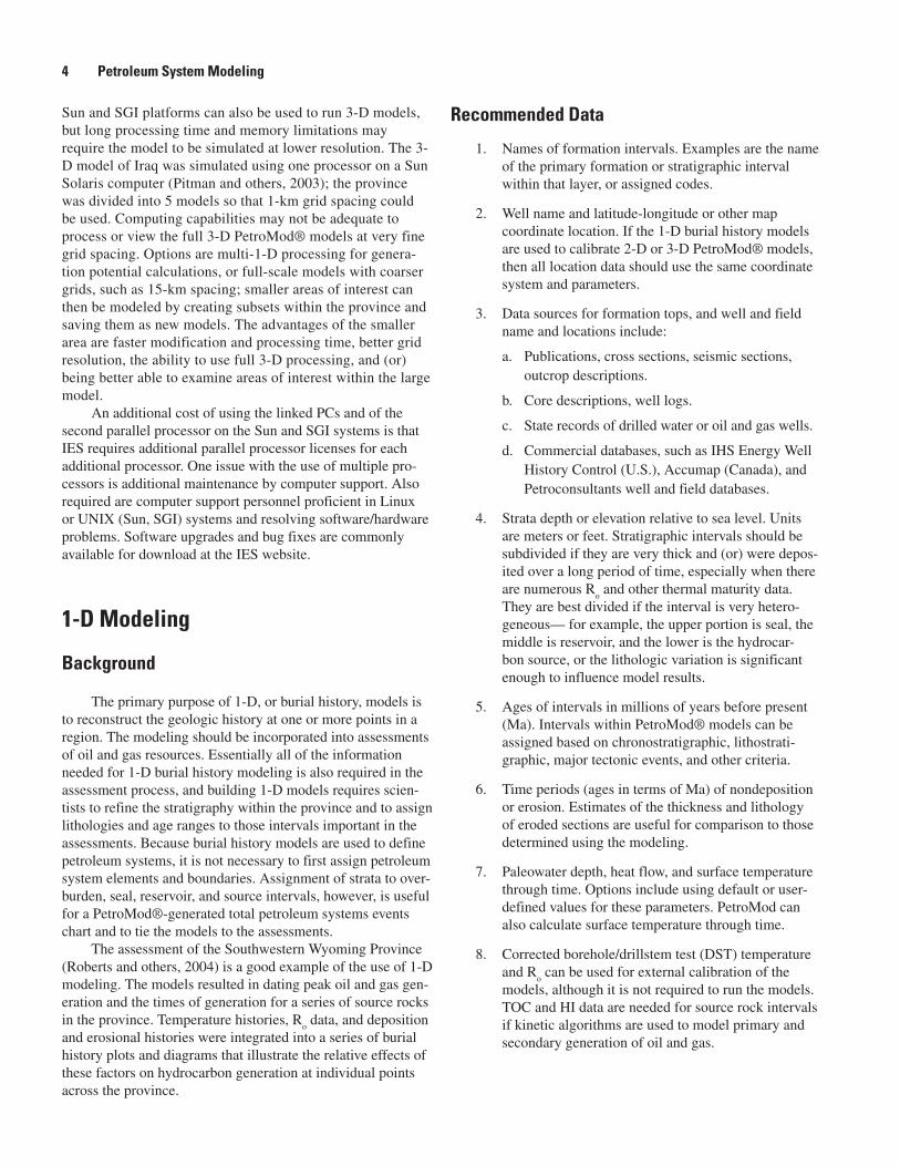
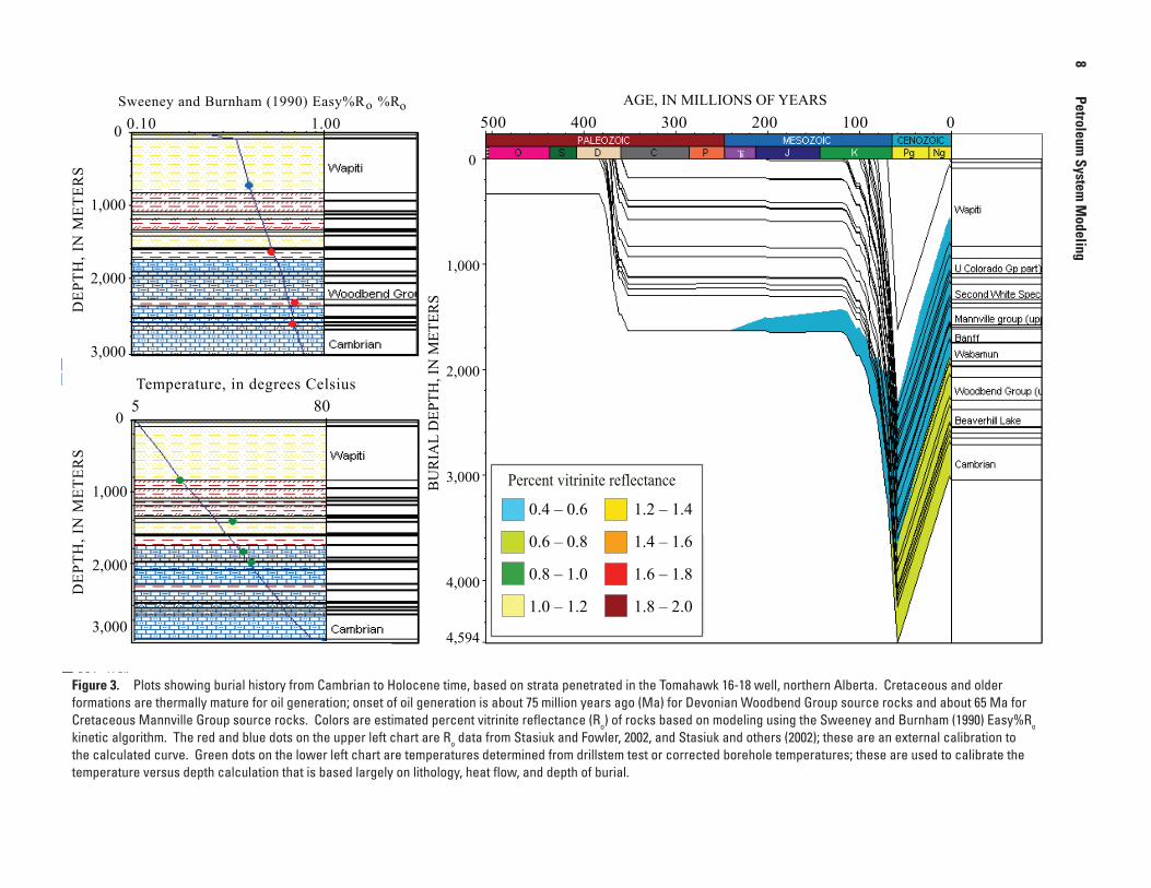
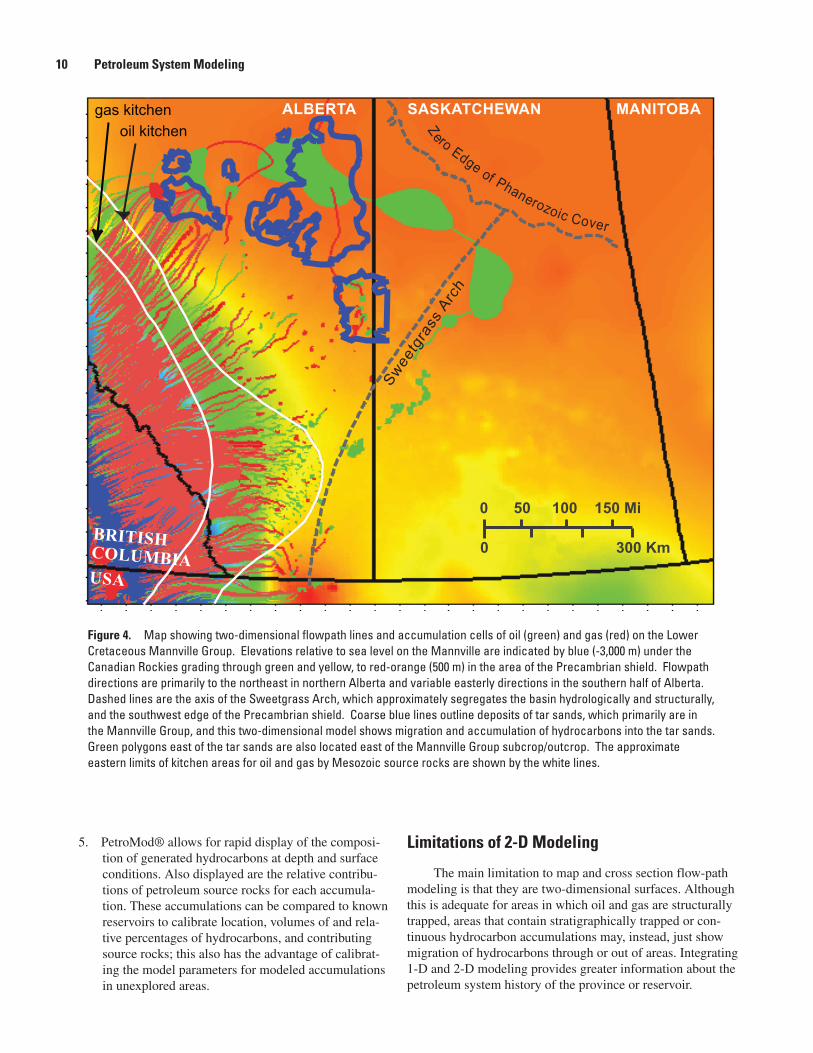
Figure 4 is a map view of a 2-D model on the top of the Lower Cretaceous Mannville Group; shown are flowpaths of oil and gas migration and accumulation. (Note: Names and lithologies of Canadian formations and groups are derived primarily from the Lexicon of Canadian Stratigraphy, 1997.) The accumulations are based on structure, however, because Mannville Group hydrocarbons are mostly stratigraphically trapped, not all accumulations are shown on the map but flowpaths through reservoir areas are displayed. Also illus-trated are oil accumulations in the areas of the major tar sand deposits. Flowpaths across layers and relative contributions of oil and (or) gas from bounding source rocks can be mod-eled in 2-D. The 3-D model of this (Mannville Group) surface differs by incorporating through time the relative contributions of all source rocks for all petroleum accumulations. Provinces or areas that have inadequate data control or quality for 3-D modeling can benefit from multiple 2-D cross sections that are located within a 3-D space. These sections provide visual and numeric information on the 3-D framework of the petroleum systems, such as influence on lithofacies and faulting on the systems, and vertical and lateral changes in hydrocarbon migration and trapping.

Recommended Data

Sources of information for generating 2-D models include well databases, 1-D burial history models, seismic sec-tions, and maps and cross sections that can contain data such as geology, topography, temperature, and pressure. Minimal information to build the models includes (1) geographic, map coordinate, or other reference locations of all data; (2) names and age ranges all layers in the model; and (3) lithologic char-acteristics of facies within the layers. Areas that are thermally mature for oil and gas can be delineated based on results of 1-D modeling and from available data. If the 2-D models are used to estimate the timing and amounts of hydrocarbon

generation, then most of the information listed in the intro-ductory section of this paper as being important to petroleum systems modeling is also required.

Time and Personnel Requirements

Time and personnel requirements for 2-D modeling are based on the time and levels of effort required to generate maps and (or) cross sections, process seismic sections, deter-mine the location and timing of faults, and evaluate kitchen areas for source rocks; all of these tasks are also needed for assessments. Actual time to create the initial PetroMod® 2-D models by an experienced user can be relatively short. However, the time required to edit the initial maps is highly variable, being dependent upon source, such as published maps or raw data, and data quality and distribution. Editing for modeling and assessment purposes can range from a day to weeks; some of this can be accomplished with GIS support staff overseen by geologists. In most cases, it probably takes less than a day to generate the edited map using EarthVision® or ARC® software, export the grid in zmap format, and create and run a 2-D map model using PetroMod®.

Advantages of Using �-D Models

Primary advantages are the following:

1. Existing structure contour map grids can be quickly converted to the IES zmap grid-file format and used as input for modeling with PetroMod®.

2. PetroMod® can directly input 2-D seismic data and interpretations from a number of formats, includ-ing sections and paleo-sections from widely-used structural modeling software packages. Travel-time conversions to depths in feet or meters should be done outside of PetroMod®. PetroMod® can also export 2-D cross sections in formats readable by some struc-tural modeling software.

3. Proprietary well data used to generate the structure and isopach maps generally cannot be published, but 2-D grid files generated from these data can be published in most cases. This has the advantage of allowing others to use the isopach and (or) structure grid files.

4. 2-D has all of the advantages of 1-D modeling, including seamless integration of 1-D and 3-D variables and parameters. Other advantages include modeling through time of PVT, salt movement, hydrodynamic flow, igneous intrusions, temperature, transformation ratios, and other factors important to hydrocarbon generation and migration.

�-D Modeling �

5. PetroMod® allows for rapid display of the composi-tion of generated hydrocarbons at depth and surface conditions. Also displayed are the relative contribu-tions of petroleum source rocks for each accumula-tion. These accumulations can be compared to known reservoirs to calibrate location, volumes of and rela-tive percentages of hydrocarbons, and contributing source rocks; this also has the advantage of calibrat-ing the model parameters for modeled accumulations in unexplored areas.

Limitations of �-D Modeling

The main limitation to map and cross section flow-path modeling is that they are two-dimensional surfaces. Although this is adequate for areas in which oil and gas are structurally trapped, areas that contain stratigraphically trapped or con-tinuous hydrocarbon accumulations may, instead, just show migration of hydrocarbons through or out of areas. Integrating 1-D and 2-D modeling provides greater information about the petroleum system history of the province or reservoir.

Sweetg

rass

Arc

h

0 300 Km

0 50 100 150 Mi

ALBERTA SASKATCHEWAN MANITOBAgas kitchen oil kitchen Zero Edge of Phanerozoic Cover

BRITISH COLUMBIAUSA

Figure �. Map showing two-dimensional flowpath lines and accumulation cells of oil (green) and gas (red) on the Lower Cretaceous Mannville Group. Elevations relative to sea level on the Mannville are indicated by blue (-3,000 m) under the Canadian Rockies grading through green and yellow, to red-orange (500 m) in the area of the Precambrian shield. Flowpath directions are primarily to the northeast in northern Alberta and variable easterly directions in the southern half of Alberta. Dashed lines are the axis of the Sweetgrass Arch, which approximately segregates the basin hydrologically and structurally, and the southwest edge of the Precambrian shield. Coarse blue lines outline deposits of tar sands, which primarily are in the Mannville Group, and this two-dimensional model shows migration and accumulation of hydrocarbons into the tar sands. Green polygons east of the tar sands are also located east of the Mannville Group subcrop/outcrop. The approximate eastern limits of kitchen areas for oil and gas by Mesozoic source rocks are shown by the white lines.

10 Petroleum System Modeling

�-D Modeling

Background3-D modeling involves reconstructing the history of

petroleum systems at reservoir to basin scales and includes the ability to display that information in 1-D, 2-D and 3-D space and through time. The models can be constructed as time-stratigraphic intervals, or delineated based on common formations or facies. Numerous variables are integrated and analyzed by the 3-D petroleum systems modeling software. These data and interpretations greatly augment the assessment of undiscovered oil and gas resources by showing the history of petroleum systems across provinces, and by analyzing the relative effects on these systems of vertical and lateral changes in lithology, heat flow, hydrodynamics, PVT behavior, and other processes. The use of 3-D petroleum systems modeling can also enhance the assessment process by providing another level of support for conclusions from the assessments. Exam-ples of this support include exclusion of areas and petroleum systems from assessment because source rocks are immature or overmature for petroleum generation, including these for-mations and areas because the modeling shows migration of petroleum from mature areas, and timing onset of petroleum generation relative to trap formation.

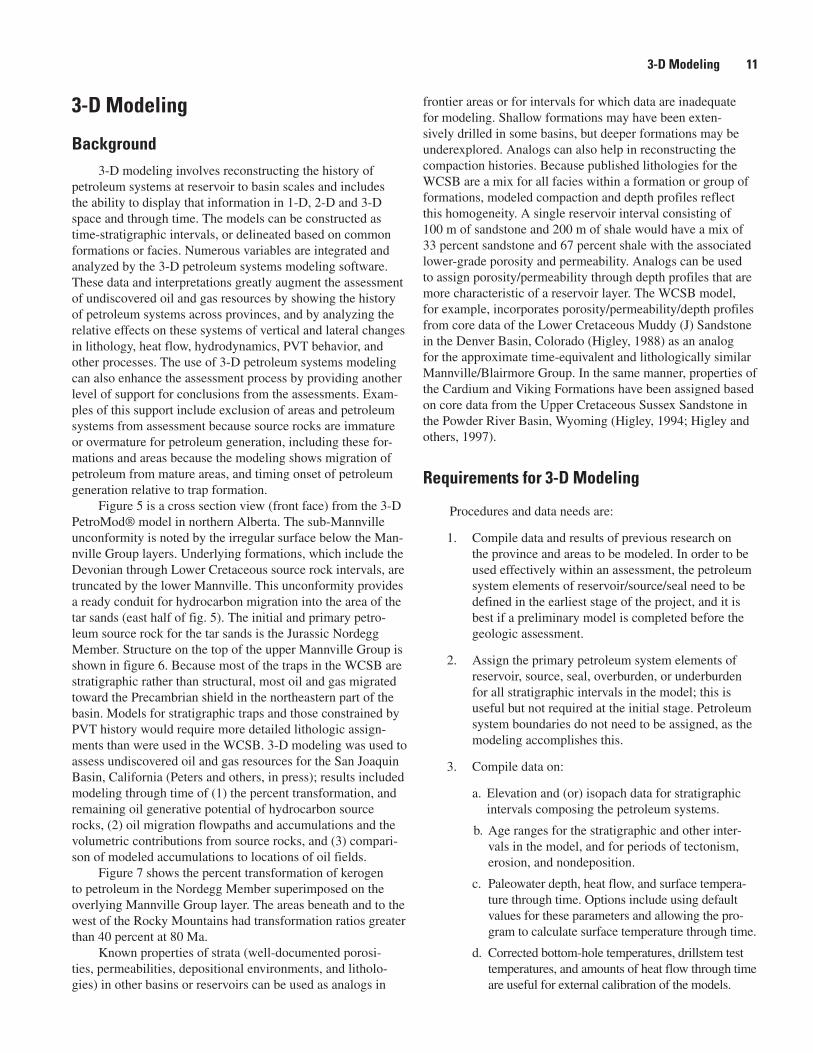
Figure 5 is a cross section view (front face) from the 3-D PetroMod® model in northern Alberta. The sub-Mannville unconformity is noted by the irregular surface below the Man-nville Group layers. Underlying formations, which include the Devonian through Lower Cretaceous source rock intervals, are truncated by the lower Mannville. This unconformity provides a ready conduit for hydrocarbon migration into the area of the tar sands (east half of fig. 5). The initial and primary petro-leum source rock for the tar sands is the Jurassic Nordegg Member. Structure on the top of the upper Mannville Group is shown in figure 6. Because most of the traps in the WCSB are stratigraphic rather than structural, most oil and gas migrated toward the Precambrian shield in the northeastern part of the basin. Models for stratigraphic traps and those constrained by PVT history would require more detailed lithologic assign-ments than were used in the WCSB. 3-D modeling was used to assess undiscovered oil and gas resources for the San Joaquin Basin, California (Peters and others, in press); results included modeling through time of (1) the percent transformation, and remaining oil generative potential of hydrocarbon source rocks, (2) oil migration flowpaths and accumulations and the volumetric contributions from source rocks, and (3) compari-son of modeled accumulations to locations of oil fields.

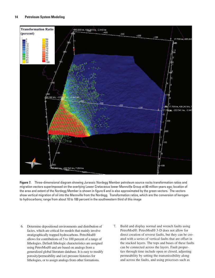
Figure 7 shows the percent transformation of kerogen to petroleum in the Nordegg Member superimposed on the overlying Mannville Group layer. The areas beneath and to the west of the Rocky Mountains had transformation ratios greater than 40 percent at 80 Ma.

Known properties of strata (well-documented porosi-ties, permeabilities, depositional environments, and litholo-gies) in other basins or reservoirs can be used as analogs in

frontier areas or for intervals for which data are inadequate for modeling. Shallow formations may have been exten-sively drilled in some basins, but deeper formations may be underexplored. Analogs can also help in reconstructing the compaction histories. Because published lithologies for the WCSB are a mix for all facies within a formation or group of formations, modeled compaction and depth profiles reflect this homogeneity. A single reservoir interval consisting of 100 m of sandstone and 200 m of shale would have a mix of 33 percent sandstone and 67 percent shale with the associated lower-grade porosity and permeability. Analogs can be used to assign porosity/permeability through depth profiles that are more characteristic of a reservoir layer. The WCSB model, for example, incorporates porosity/permeability/depth profiles from core data of the Lower Cretaceous Muddy (J) Sandstone in the Denver Basin, Colorado (Higley, 1988) as an analog for the approximate time-equivalent and lithologically similar Mannville/Blairmore Group. In the same manner, properties of the Cardium and Viking Formations have been assigned based on core data from the Upper Cretaceous Sussex Sandstone in the Powder River Basin, Wyoming (Higley, 1994; Higley and others, 1997).

Requirements for �-D Modeling

Procedures and data needs are:

1. Compile data and results of previous research on the province and areas to be modeled. In order to be used effectively within an assessment, the petroleum system elements of reservoir/source/seal need to be defined in the earliest stage of the project, and it is best if a preliminary model is completed before the geologic assessment.

2. Assign the primary petroleum system elements of reservoir, source, seal, overburden, or underburden for all stratigraphic intervals in the model; this is useful but not required at the initial stage. Petroleum system boundaries do not need to be assigned, as the modeling accomplishes this.

3. Compile data on:

a. Elevation and (or) isopach data for stratigraphic intervals composing the petroleum systems.

b. Age ranges for the stratigraphic and other inter-vals in the model, and for periods of tectonism, erosion, and nondeposition.

c. Paleowater depth, heat flow, and surface tempera-ture through time. Options include using default values for these parameters and allowing the pro-gram to calculate surface temperature through time.

d. Corrected bottom-hole temperatures, drillstem test temperatures, and amounts of heat flow through time are useful for external calibration of the models.

�-D Modeling 11

Mannville and unconformityNordeggDoig

ExshawDuvernay

2nd White Sp.

North

Figure �. East-west cross section across northern Alberta includes all layers in the 3-D model. Location of section and association to tar sands of the Mannville Group are shown in figure 6. The Jurassic layer (blue) and included Nordegg Member are truncated by the Mannville Group layer. Nordegg high-sulfur type II kerogen shale is the initial source of hydrocarbons for the tar sands. Later contributors of hydrocarbons are the Triassic Doig and Mississippian Exshaw shales, and low-sulfur carbonates of the Duvernay Member of the Woodbend Group. The 2nd White Speckled Shale was isolated from the Mannville petroleum system by shales of the Joli Fou and lower Colorado Group.

e. Locations and ages of faulting; timing of when the faults and segments were open or closed.

f. Lateral and vertical distribution of depositional facies/lithology from maps, cross sections, andwritten descriptions.

g. Information useful for modeling changes through time, such as (1) paleogeometry maps to show influence of depositional or tectonic effects on the geometry of the interval and model, (2) location of salt diapirs for determination of salt movement, (3) igneous intrusions, (4) hydrodynamic movement, (5) pressure-boundary conditions, and (6) gas hydrates.

1� Petroleum System Modeling

0 200 KM

0 100 200 Mi

BC Alberta Saskatchewan

USA

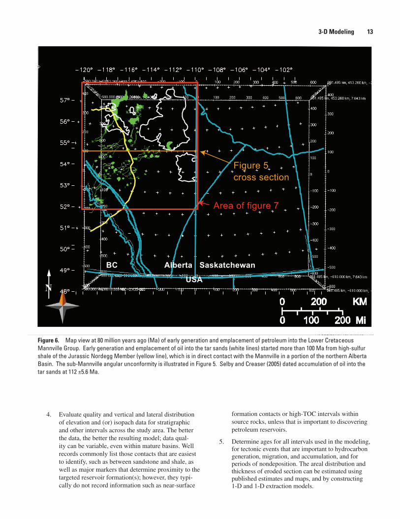
Area of figure 7

Figure 5 cross section

N

Figure �. Map view at 80 million years ago (Ma) of early generation and emplacement of petroleum into the Lower Cretaceous Mannville Group. Early generation and emplacement of oil into the tar sands (white lines) started more than 100 Ma from high-sulfur shale of the Jurassic Nordegg Member (yellow line), which is in direct contact with the Mannville in a portion of the northern Alberta Basin. The sub-Mannville angular unconformity is illustrated in Figure 5. Selby and Creaser (2005) dated accumulation of oil into the tar sands at 112 ±5.6 Ma.

4. Evaluate quality and vertical and lateral distribution of elevation and (or) isopach data for stratigraphic and other intervals across the study area. The better the data, the better the resulting model; data qual-ity can be variable, even within mature basins. Well records commonly list those contacts that are easiest to identify, such as between sandstone and shale, as well as major markers that determine proximity to the targeted reservoir formation(s); however, they typi-cally do not record information such as near-surface

formation contacts or high-TOC intervals within source rocks, unless that is important to discovering petroleum reservoirs.

5. Determine ages for all intervals used in the modeling, for tectonic events that are important to hydrocarbon generation, migration, and accumulation, and for periods of nondeposition. The areal distribution and thickness of eroded section can be estimated using published estimates and maps, and by constructing 1-D and 1-D extraction models.

�-D Modeling 1�

6. Determine depositional environments and distribution of facies, which are critical for models that mainly involve stratigraphically trapped hydrocarbons. PetroMod® allows for contributions of 5 to 100 percent of a range of lithologies. Default lithologic characteristics are assigned using PetroMod® and are based on analogs from a generalized global literature database. It is easy to modify porosity/permeability and (or) pressure histories for lithologies, or to assign analogs from other formations.

7. Build and display normal and wrench faults using PetroMod®. PetroMod® 3-D does not allow for direct creation of reverse faults, but they can be cre-ated with a series of vertical faults that are offset in the stacked layers. The tops and bases of these faults can be connected across the layers. Fault proper-ties through time include open or closed, adjusting permeability by setting the transmissibility along and across the faults, and using processes such as

Transformation Ratio (percent)

Figure �. Three-dimensional diagram showing Jurassic Nordegg Member petroleum source rocks transformation ratios and migration vectors superimposed on the overlying Lower Cretaceous lower Mannville Group at 80 million years ago; location of the area and extent of the Nordegg Member is shown in figure 6 and is also approximated by the green vectors. The vectors show vertical migration of oil into the Mannville from the Nordegg. Transformation ratios, which are the conversion of kerogen to hydrocarbons; range from about 10 to 100 percent in the southwestern third of this image

1� Petroleum System Modeling

assigning lithologic properties along the fault traces, or by direct assignment of shale-gouge ratio (SGR) maps to faults. Examples of lithologic assignments are shale for use as fault gouge, or anhydrite for a closed fault.

8. Compile data on TOC and HI for source intervals in the model; these are required sources of carbon and hydro-gen that are needed for the model to generate oil and gas. Default values and analogs of these data can be used.

9. Compile Ro data, useful for external calibration

of 3-D models. The modeling software includes numerous algorithms for calculating and calibrating thermal maturation through time. The model can also be calibrated using 1-D burial histories of wells, and 1-D extractions of 3-D models.

10. Select kinetics algorithms for use in modeling the timing of hydrocarbon generation. The program allows for use of default or input of user-defined kinetic parameters for primary generation and second-ary cracking of oil and gas. Necessary information on source rocks that contribute hydrocarbons to each petroleum system includes their lateral and vertical distribution, kerogen type, lithology, TOC, and HI. Timing of generation of hydrocarbons is dependent upon choice of petroleum kinetic algorithms.

Time and Personnel Requirements

Building 3-D models of petroleum systems ideally requires staff with backgrounds in data management, geology, geophysics, organic geochemistry, and use of modeling soft-ware. If 3-D modeling is to be incorporated into an assessment, the province first needs to be evaluated based on whether the available data, in terms of type, quality, and distribution, are suitable for the modeling or whether analogs are necessary. The assessment may not require modeling the entire basin, but may instead benefit from one or more models in selected areas of the province; this requires that kitchen area(s) be located within the subsets. In any case, the modeling should start before initiating the geologic assessment itself, preferably soon fol-lowing compilation of basic well, lithologic, map, and thermal maturation information. Even if the data collection, mapping, and model construction is completed within a year, it can take additional time to refine the model and its contained parts, and to evaluate all the results and apply them to the geologic assess-ment, which precedes assessment of undiscovered resources.

Models should be built by geoscientists that are fairly computer literate. The USGS Energy Team has geoscientists in both Denver and Menlo Park offices that have experience building 3-D models. However, IES PetroMod® 3-D currently has limited documentation and tutorials, so initial training was done using IES personnel; training is increasingly being given by Energy Team personnel. Much of the training in 3-D is hands-on and requires considerable time to learn the complex

and extensive functions of the software. IES personnel have also helped in construction and review of the 3-D models.

Advantages of �-D Models

The primary advantages of 3-D modeling are:

1. Reservoir- to basin-scale reconstructions can show hydrocarbon migration into areas that are unexplored or underexplored. An example of this is the northern WCSB, where there is a migration and accumula-tion pathway across the Lower Cretaceous Mannville Sandstone into the Precambrian Shield area. Although potential reservoirs there are removed by erosion, Lloyd Snowdon (oral commun., June 10, 2004), formerly of the Canada Geological Survey, indicated that some Mannville outcrops along the pathway are saturated with bitumen.

2. Oil and gas generation, migration, and accumulation are modeled through time. The volumes of in-place, generated, accumulated, and lost oil and gas can be calculated and displayed through time for each petro-leum system. Flash calculation charts and numbers generated by the modeling software show these gen-erated volumes at surface conditions. Flash numbers allow for a better comparison of modeled numbers to produced and in-place oil and gas.

3. Numerous processes that affect petroleum system elements also change through time, and these changes can be integrated into the model, including those involving salt movement, open and closed normal faults, wrench and other types of faults, hydrodynam-ics, paleogeometry, igneous intrusions, permafrost, and clathrates.

4. Multicomponent PVT analysis incorporates changes due to compaction, temperature, faulting, heating history, and other variables. Output includes PVT history, including fault and formation capillary, lithologic, and other types of pressure, shale gouge ratio, and various hydrocarbon and non-hydrocarbon components, such as carbon dioxide and nitrogen. Calculated are the volume, composition, density, and viscosity of liquid, vapor, and water phases.

5. The PetroRisk risking module can be applied at 1-D, 2-D, and 3-D scales. Risk analysis within the 3-D modeling allows uncertainties in the geologic/geo-chemical data to be assigned and the effects of these uncertainties can be analyzed and compared through multiple runs using Monte Carlo or Latin Hypercube sampling techniques and multiple simulations. The risking can be performed on the petroleum charge, generation, migration, and loss calculations.

�-D Modeling 1�

6. PetroMod® calculates the relative percent and volumetric contribution of gas through heavy oil from each source rock at reservoir, interval, and basin scales. This identifies the primary source rocks and their relative contributions through time at accumula-tion to province scales. Mature basins allow better evaluations and calibrations of models by compar-ing the calculated volumes to known volumes of in-place and recoverable oil and gas and estimates of undiscovered resources. This type of analysis is both for training purposes and for later use of the models as analogs for other basins or reservoirs. Volumes of generated hydrocarbons can be calculated by the modeling software, although these numbers can differ considerably from estimated volumes of in-place, discovered, or undiscovered hydrocarbons. Instead of publishing volumes of generated and accumulated hydrocarbons, it is preferable to publish the percent contribution of each source rock for the because of; (a) Differences between the volumes of generated, migrated, and accumulated hydrocarbons; (b) the effects of grid resolution on the locations and vol-umes of accumulated hydrocarbons, especially since grid cells can be considerably larger than the sizes of modeled and real accumulations; (c) inadequate geologic/geochemical information about the vertical and lateral extent and richness of source rocks; (d) information regarding lithologic characteristics of reservoir, source, and seal are generalized; and (e) a number of other parameters are generalized in the modeling due to insufficient data. A primary param-eter is the quality of the source rocks, which vary in organic richness vertically and laterally. Although TOC, R

o, and similar data may be available at point

sources within study areas, the modeling involves extrapolating the TOC and other information over broad vertical and lateral areas.

7. PetroReport® produces graphs and tables that display the temporal evolution of relative contributions of hydrocarbons from source rocks at both for in-place and flashed-to-surface conditions. Reported volumes are also divided into generated, inflow and outflow, adsorbed, and within the water phase. This calcula-tion and display is done at accumulation to basin scales. Calculations of the total hydrocarbon volumes are suspect because they are influenced by so many variables; for this reason a risk analysis should be performed to assess the distribution ranges, prob-abilities, and sensitivities of the results. However the relative volume percentages from each source provide a check of the reliability of modeling factors such as kinetics, TOC and HI values, assigned lithologies and associated porosity/permeability characteriza-tions, interval thickness and distribution, and pressure history. The graphs and tables can further be used

to check against 1-D and published information on timing and sources of hydrocarbon generation for reservoir intervals.

8. 3-D modeling can incorporate Darcy (vertical), flow-path (lateral), or hybrid Darcy (vertical and lateral) fluid flow.

9. Because of the data, time, and personnel require-ments for full 3-D modeling, there is the option of using small sub-sets of areas within the models that have good seismic and (or) well coverage. Sub-sets can be processed at finer grid spacing that most basin models allow, and the resulting model can be used as on its own merit, or as an analog for other areas of the province. This is useful if there is an area of particu-lar importance within a province.

10. Modeling changes in pressure history both laterally and vertically is an effective research tool for uncon-ventional resources. Modeled processes include effects on pressure due to mechanical and chemical compac-tion and fluid expansion. Influences through time on gas trapping and interplay of capillary pressure, changes in porosity and permeability for lithologies, and sealing capacities can be incorporated, and the effects of underpressured or overpressured zones on degree and timing of trapping can also be evaluated.

11. A 3-D model includes hydrocarbon phase behavior (liquid, vapor). PetroMod® further calculates and reports the gas-oil ratio (GOR), API gravity, and composition and relative percentage of these liquids and vapors, such as C3-C5, C15 plus aromatics, C15 plus saturated hydrocarbons, and water. These values can also be flashed to surface conditions for compari-son to produced volumes and compositions.

12. PetroMod® serves as an archive for assigned parameters because they are tabulated within each 1-D, 2-D, and 3-D model. The 3-D model, and each contained 2-D grid file and associated metadata can be published for use by other scientists.

Requirements and Limitations of �-D Modeling

The primary disadvantage of 3-D modeling is that it requires considerable data, personnel, training, time, and com-puter processing capabilities. One of the greatest deterrents within the USGS Energy Team is the limited number of geo-scientists and support personnel trained in assessment method-ology, petroleum systems, and the use of modeling software. Construction of a 3-D basin model can take a year or more to complete and evaluate for use in geologic and resource assessments. Most of this time is used for background research on the province, and compiling the geologic and geochemical data for the modeling; this information is also critical for the

1� Petroleum System Modeling

assessments. Time can be saved by building smaller models for areas within the province for use as analogs. The following are requirements for the 3-D modeling.

1. Ample personnel and computer time and equipment need to be dedicated to build the models. Although models can run using PC, SUN, and IRIX platforms, compared to Linux clusters of PCs these tend to be very slow and more prone to crash due to memory handling and limitations. The models also require many gigabytes of storage space. Storage space, memory, and processing ability also determine the choice of resolution that can be processed and dis-played of the models.

2. Considerable data are required for a full 3-D model, and data quality and distribution are critical.

3. Main disadvantage of risk analysis using the PetroRisk® software is it can require long processing times.

4. Modeling software can change significantly with new versions; generally these are improvements but updat-ing the model can modify the results.

Conclusions

It is necessary to continually improve our methodology for assessing conventional and unconventional resources. 1-D, 2-D, and 3-D petroleum systems models within provinces are used to (1) build and evaluate the hydrocarbon history for potential source and reservoir rocks, and (2) document time periods of deposition, erosion, and tectonic events and assess their relative influences on petroleum generation, migration, and accumula-tion. Unconventional resources can also be evaluated using multicomponent pressure, volume, temperature (PVT) analy-sis that models changes in these variables through time based on thermal history, vertical and lateral changes in lithologies, changes in pressure associated with oil and gas generation and secondary cracking. PVT analysis incorporates various hydro-carbon components, and includes carbon dioxide and nitrogen.

Models are powerful tools that assist in (1) defining petroleum system elements and boundaries, (2) determin-ing the timing of hydrocarbon generation and migration and of trap formation, (3) displaying and documenting 2-D and 3-D flow of hydrocarbons within and across petroleum systems, (4) evaluating relative contributions of source rocks to reservoir intervals, and (5) modeling influences on hydrocarbon migration of open and closed fault systems, salt movement, and other variables. 1-D and 2-D petroleum systems models are relatively easy to learn and rapid to build. The required data are generally available for resource assessments, and the models are small enough to be built and saved on a variety of computer platforms and storage

devices. 3-D models can be created at reservoir to basin scales; subsets within provinces can be built as separate models or dissected from the full 3-D model. In order to be used most effectively, the models should be built before the geologic and resource assessments.

Acknowledgements

This paper was prepared as a white paper for Brenda Pierce, Program Coordinator for the Energy Resources Pro-gram of the U.S. Geological Survey for the purpose of evaluat-ing the use of 1-D, 2-D, and 3-D petroleum systems modeling in the assessment of undiscovered oil and gas resources. We benefited greatly from the reviews and helpful comments by William Keefer, Allegra Hosford Scheirer, Janet Pitman, Mark Pawlewicz, Mahendra Verma, and Daniel Hayba of the U.S. Geological Survey, and Bjorn Wygrala of Integrated Explora-tion Systems (IES).

References

Adams , J., Rostron, B.J., and Mendoza, C.A., 2000, Regional fluid flow and the Athabasca oil sands: numerical simula-tions using a fully-coupled heat solute and groundwater flow model. Paper 476, GeoCanada 2000, Joint Annual Meeting of GAC,MAC, CWLS, CGU, CSEG, and CSPG, Calgary, May 29-June 2, 2000, 4 p.

Bekele, E.B., Person, M.A., Rostron, B.J., and Barnes, R., 2002, Modeling secondary oil migration with core-scale data: Viking Formation, Alberta Basin: American Asso-ciation of Petroleum Geologists Bulletin, v. 86, no. 1, p. 55–74.

Creaney, S. and J. Allen, 1990, Hydrocarbon generation and migration in the Western Canada Sedimentary Basin, in Brooks, J., ed., Classic Petroleum Provinces, 1990, London, The Geological Society, p. 189-202.

Creaney, S., and J. Allan, 1992, Petroleum systems in the foreland basin of Western Canada, in Macqueen, R.W., and Leckie, D.A., eds., Foreland basins and fold belts: American Association of Petroleum Geologists Memoir 55, p. 279-308.

Deming, David, 1994, Overburden rock, temperature, and heat flow; Magoon, L.B. and Dow, W.G., eds., The petroleum system – from source to trap: American Association of Petroleum Geologists Memoir 60, p 165–186.

Dynamic Graphics Corporation, 2005, EarthVision software: Dynamic Graphics Corporation, 1015 Atlantic Avenue, Alameda, California. http://www.dgi.com

References 1�

Fowler, M., and Riediger, C., 2000, Stop 14 – Origin of the Athabasca tar sands, in Barson, D. Bartlett, R., Hein, F., Fowler, M., Grasby, S., Riediger, C., and Underschultz, J., eds., 2000, Hydrogeology of heavy oil and tar sand depos-its: Water flow and supply, migration and degradation: Geological Survey of Canada, Open-File Report No. 3946.

Integrated Exploration Services, 2005, PetroMod® Basin and Petroleum Systems Modeling Software: IES GmbH, Ritter-str, 23, 52072 Aachen, Germany, http://www.ies.de

IHS Energy Accumap database, 2004, available from IHS Energy, 4100 Dry Creek Road, Littleton, Colorado 80122.

IHS Energy Well History Control System database, 2004, available from IHS Energy, 4100 Dry Creek Road, Littleton, Colorado 80122.

Higley, D. K., 1988, Core porosity, permeability, and vitrinite reflectance data from the Lower Cretaceous J sandstone in 141 Denver Basin coreholes; U.S. Geological Survey Open-File Report 88–527, 6 p., 2 floppy diskettes.

Higley, D.K., 1994, Three-dimensional flow-unit characteriza-tion of a transgressive marine sand-ridge complex, Upper Cretaceous Sussex “B” sandstone, House Creek oil field, Wyoming: Colorado School of Mines Ph.D. dissertation, 334 p., 1 diskette, 12 plates.

Higley, D.K., Pantea, M.P., and Slatt, R.M., 1997, 3-D reser-voir characterization of the House Creek oil field, Powder River Basin, Wyoming, V 1.00: U.S. Geological Survey Digital Data Series 33, 200 MB. http://pubs.usgs.gov/dds/dds-033/USGS_3D/homepage.htm (last accessed 1/24/06)

Higley, D.K., Henry, M, Lewan, M., and Pitman, J., 2003, Material balance assessment of the New Albany Shale petroleum system, Illinois Basin, Illinois, Indiana, and Kentucky - data and map image archive, V 1.00: U.S. Geological Survey Open-File Report OF-03-037, 45 p., 19 figures, 2 tables, 2 appendices. http://pubs.usgs.gov/of/2003/ofr-03-037/ (last accessed 3/05)

Higley, Debra K., Cook, Troy A., Pollastro, Richard M., Charpentier, Ronald R., Klett, Timothy R., and Schenk, Christopher J., 2005, Assessment of Undiscovered Oil and Gas Resources of the Raton Basin – Sierra Grande Uplift Province of New Mexico and Colorado, 2004: U.S. Geo-logical Survey Fact Sheet 2005-3027, 2 p.

Higley, Debra K., Henry, Mitchell, Roberts, Laura N.R., and Steinshouer, Douglas W., 2005, 1-D/3-D Geologic Model of the Western Canada Sedimentary Basin: The Mountain Geologist, v. 42, no. 2, p. 53–66.

Lewan, M. D., Henry, M.E., Higley, D.K., and Pitman, J.K., 2002, Material-balance assessment of the New Albany-Chesterian petroleum system of the Illinois Basin: Ameri-can Association of Petroleum Geologists Bulletin, v. 86, no. 5, p. 745–777.

Lexicon of Canadian Stratigraphy, volume 4, Western Canada, 1997, Glass, D.J., ed.: Canadian Society of Petroleum Geologists, 1,423 pg, 1 pdf-format document.

Magoon, L.B., and Dow, W.G., 1994, The petroleum system, in Magoon, L.B., and Dow, W.G., eds., The Petroleum System – From source to trap: American Association of Petroleum Geologists Memoir 60, p. 3-23.

Magoon, L.B., and Schmoker, J.W., 2000, The total petro-leum system – the natural fluid network that constrains the assessment unit, in U.S. Geological Survey World Petroleum Assessment 2000 – description and results: U.S. Geological Survey DDS–60, p. PS-1–PS-20, 1–5.

Moshier, S.O., and Waples, D.W., 1985, Quantitative evalua-tion of Lower Cretaceous Mannville Group as source rock for Alberta’s oil sands: American Association of Petroleum Geologists Bulletin, v. 69, no. 2, p. 161–172

Pitman, Janet K., Steinshouer, Douglas W., and Lewan, Michael D., 2003, Generation and migration of petroleum in Iraq: a 2 1/2-D and 3-D modeling study of Jurassic source rocks: U.S. Geological Survey Open-File Report 03-192, 17p. http://pubs.usgs.gov/of/2003/ofr-03-192/ (last accessed 03/05).

Roberts, Laura N.R., Lewan, Michael D., and Finn, Thomas M., 2004, Timing of oil and gas generation of petroleum systems in the southwestern Wyoming Province: Rocky Mountain Association of Geologists Mountain Geologist, v. 41, p. 87-118.

Selby, David, and Creaser, Robert, 2005, Direct radiometric dating of hydrocarbon deposits using rhenium-osmium isotopes: Science, v. 308, May 27, p. 1293-1295.

Stasiuk, L.D., and Fowler, M.G., 2002, Thermal maturity evaluation (vitrinite and vitrinite reflectance equivalent) of Middle Devonian, Upper Devonian, and Mississippian strata in the Western Canada Sedimentary Basin: Geological Survey of Canada Open-File 4341, 1 CD-ROM.

Stasiuk, L.D., Fowler, M.G., and Addison, 2002, Thermal maturity evaluation of Lower Cretaceous Mannville Group and equivalent coals in the Western Canada Sedimentary Basin; a compilation of vitrinite reflectance data: Geologi-cal Survey of Canada Open-File 4342, 1 CD-ROM.

Sweeney, J.J., and A.K. Burnham, 1990, Evaluation of a simple model of vitrinite reflectance based on chemical kinetics: American Association of Petroleum Geologists Bulletin, v. 74, p. 1,559-1,570.

1� Petroleum System Modeling