Pessimistic Cardinality Estimation: Tighter UpperBounds for Intermediate Join CardinalitiesWalter Cai

University of Washington

Seattle, Washington

walter@cs.washington.edu

Magdalena Balazinska

University of Washington

Seattle, Washington

magda@cs.washington.edu

Dan Suciu

University of Washington

Seattle, Washington

suciu@cs.washington.edu

ABSTRACTIn this work we introduce a novel approach to the prob-

lem of cardinality estimation over multijoin queries. Our

approach leveraging randomized hashing and data sketching

to tighten these bounds beyond the current state of the art.

We demonstrate that the bounds can be injected directly

into the cost based query optimizer framework enabling it

to avoid expensive physical join plans. We outline our base

data structures and methodology, and how these bounds

may be introduced to the optimizer’s parameterized cost

function as a new statistic for physical join plan selection.

We demonstrate a complex tradeoff space between the tight-

ness of our bounds and the size and complexity of our data

structures. This space is not always monotonic as one might

expect. In order combat this non-monotonicity, we introduce

a partition budgeting scheme that guarantees monotonic be-

havior. We evaluate our methods on GooglePlus community

graphs [11], and the Join Order Benchmark (JOB) [16]. In

the presence of foreign key indexes, we demonstrate a 1.7×improvement in aggregate (time summed over all queries

in benchmark) physical query plan runtime compared to

plans chosen by Postgres using the default cardinality esti-

mation methods. When foreign key indexes are absent, this

advantage improves to over 10×.

ACM Reference Format:Walter Cai, Magdalena Balazinska, and Dan Suciu. 2019. Pessimistic

Cardinality Estimation: Tighter Upper Bounds for Intermediate Join

Cardinalities. In 2019 International Conference on Management ofData (SIGMOD ’19), June 30-July 5, 2019, Amsterdam, Netherlands.ACM,NewYork, NY, USA, 18 pages. https://doi.org/10.1145/3299869.

3319894

Permission to make digital or hard copies of all or part of this work for

personal or classroom use is granted without fee provided that copies are not

made or distributed for profit or commercial advantage and that copies bear

this notice and the full citation on the first page. Copyrights for components

of this work owned by others than ACMmust be honored. Abstracting with

credit is permitted. To copy otherwise, or republish, to post on servers or to

redistribute to lists, requires prior specific permission and/or a fee. Request

permissions from permissions@acm.org.

SIGMOD ’19, June 30-July 5, 2019, Amsterdam, Netherlands© 2019 Association for Computing Machinery.

ACM ISBN 978-1-4503-5643-5/19/06. . . $15.00

https://doi.org/10.1145/3299869.3319894

▷◁

▷◁

▷◁

(a) Left Deep

▷◁

▷◁ ▷◁

(b) Bushy

▷◁

▷◁

▷◁

(c) Right Deep

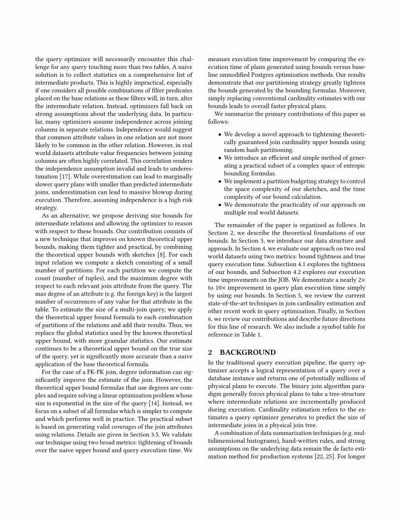
Figure 1: Join tree illustration where nodes representrelations. Intermediate relations highlighted in red.

1 INTRODUCTIONCost based query optimizers use complex parameterized for-

mulas to estimate the cost of candidate physical join plans.

When presented with a multijoin query, most systems still

rely on binary join algorithms to iteratively join these ta-

bles one-by-one into one or several growing intermediate

relations. Figure 1 highlights these intermediate relations

in red. A fundamental parameter to the formulas is the esti-

mated size of these intermediate relations. If accurate row

counts are available, there formulas generally avoid poor

plans. However, when estimates are poor, the plan selection

process becomes unreliable. Most optimizers have sophisti-

cated methods of estimating selectivity of filter predicates

applied to a single relation, but fall back on strong assump-

tions about the underlying data to handle join predicates.

In this paper we focus on multijoin queries and the risks of

intermediate relation blowup. Whereas key-foreign-key (K-

FK) joins cannot exceed the size of the foreign key relation,

queries threaten blowup when FK columns in two relations

are joined. In the FK-FK join scenario, the resulting interme-

diate relation will often be many times larger –or even many

degrees of magnitude larger– than the base relations.

Most production systems keep summary data (i.e. his-

tograms, samples, other statistics) on base relations and use

these to estimate the size of joins directly involving base

relations, i.e. nodes whose two children are both base re-

lations. However, it is difficult to reason about the size of

final or intermediate relations when one or both of the child

relations is itself an intermediate relation. Unfortunately,

the query optimizer will necessarily encounter this chal-

lenge for any query touching more than two tables. A naive

solution is to collect statistics on a comprehensive list of

intermediate products. This is highly impractical, especially

if one considers all possible combinations of filter predicates

placed on the base relations as these filters will, in turn, alter

the intermediate relation. Instead, optimizers fall back on

strong assumptions about the underlying data. In particu-

lar, many optimizers assume independence across joining

columns in separate relations. Independence would suggest

that common attribute values in one relation are not more

likely to be common in the other relation. However, in real

world datasets attribute value frequencies between joining

columns are often highly correlated. This correlation renders

the independence assumption invalid and leads to underes-

timation [17]. While overestimation can lead to marginally

slower query plans with smaller than predicted intermediate

joins, underestimation can lead to massive blowup during

execution. Therefore, assuming independence is a high risk

strategy.

As an alternative, we propose deriving size bounds for

intermediate relations and allowing the optimizer to reason

with respect to these bounds. Our contribution consists of

a new technique that improves on known theoretical upper

bounds, making them tighter and practical, by combining

the theoretical upper bounds with sketches [8]. For each

input relation we compute a sketch consisting of a small

number of partitions. For each partition we compute the

count (number of tuples), and the maximum degree with

respect to each relevant join attribute from the query. The

max degree of an attribute (e.g. the foreign key) is the largest

number of occurrences of any value for that attribute in the

table. To estimate the size of a multi-join query, we apply

the theoretical upper bound formula to each combination

of partitions of the relations and add their results. Thus, we

replace the global statistics used by the known theoretical

upper bound, with more granular statistics. Our estimate

continues to be a theoretical upper bound on the true size

of the query, yet is significantly more accurate than a naive

application of the base theoretical formula.

For the case of a FK-FK join, degree information can sig-

nificantly improve the estimate of the join. However, the

theoretical upper bound formulas that use degrees are com-

plex and require solving a linear optimization problemwhose

size is exponential in the size of the query [14]. Instead, we

focus on a subset of all formulas which is simpler to compute

and which performs well in practice. The practical subset

is based on generating valid coverages of the join attributes

using relations. Details are given in Section 3.5. We validate

our technique using two broad metrics: tightening of bounds

over the naive upper bound and query execution time. We

measure execution time improvement by comparing the ex-

ecution time of plans generated using bounds versus base-

line unmodified Postgres optimization methods. Our results

demonstrate that our partitioning strategy greatly tightens

the bounds generated by the bounding formulas. Moreover,

simply replacing conventional cardinality estimates with our

bounds leads to overall faster physical plans.

We summarize the primary contributions of this paper as

follows:

• We develop a novel approach to tightening theoreti-

cally guaranteed join cardinality upper bounds using

random hash partitioning.

• We introduce an efficient and simple method of gener-

ating a practical subset of a complex space of entropic

bounding formulas.

• We implement a partition budgeting strategy to control

the space complexity of our sketches, and the time

complexity of our bound calculation.

• We demonstrate the practicality of our approach on

multiple real world datasets.

The remainder of the paper is organized as follows. In

Section 2, we describe the theoretical foundations of our

bounds. In Section 3, we introduce our data structure and

approach. In Section 4, we evaluate our approach on two real

world datasets using two metrics: bound tightness and true

query execution time. Subsection 4.1 explores the tightness

of our bounds, and Subsection 4.2 explores our execution

time improvements on the JOB. We demonstrate a nearly 2×

to 10× improvement in query plan execution time simply

by using our bounds. In Section 5, we review the current

state-of-the-art techniques in join cardinality estimation and

other recent work in query optimization. Finally, in Section

6, we review our contributions and describe future directions

for this line of research. We also include a symbol table for

reference in Table 1.

2 BACKGROUNDIn the traditional query execution pipeline, the query op-

timizer accepts a logical representation of a query over a

database instance and returns one of potentially millions of

physical plans to execute. The binary join algorithm para-

digm generally forces physical plans to take a tree-structure

where intermediate relations are incrementally produced

during execution. Cardinality estimation refers to the es-

timates a query optimizer generates to predict the size of

intermediate joins in a physical join tree.

A combination of data summarization techniques (e.g. mul-

tidimensional histograms), hand-written rules, and strong

assumptions on the underlying data remain the de facto esti-

mation method for production systems [22, 25]. For longer

Notation Definition

D database instance

R,R j , S,T relations

t tuple

a,ai attributes

aaa attribute sets

aaaj attributes of relation R jQ query head

H hypergraph

(u1, . . . ,um ) fractional edge cover

H hash function

W domain of attributes

[M] the set {1, . . . ,M }I hash value array where entries correspond

to attributes a ∈ aaa: I ∈ [M]|aaa |

T I, RI , RIj relation subsets corresponding to hash

value array IDI

subset of database instance corresponding

to hash value array Ic, cR , cR I count statistic

da , daR , daR I max degree statistic with respect to at-

tribute aB partition budget

h entropy

S,SR relation sample

Table 1: Symbol table.

multijoins or cyclic joins, these approaches becomes increas-

ingly inaccurate [16] and in particular gravitate towards un-

derestimation in real world settings. Underestimation leads

to poor physical plan selection, which in turn leads to poor

performance. We argue that providing guaranteed bounds

on intermediate join cardinality can make selection more

robust.

The first step towards these bounds comes from analyzing

the connection between information theory and relational

databases. Framing relational joins as hypergraphs, Atserias

et al. generate upper bounds based on fractional edge cov-

ers [4]. More formally, take a conjunctive query on relations

R1, . . . ,Rm with attribute collections aaa1, . . . ,aaam .

Q (aaa) :-R1 (aaa1) , . . . ,Rm (aaam )

where aaa = ∪jaaaj . We define a hypergraph H which models

the schema of the query. A hypergraph is a generalization of

an undirected graph where the hyperedges of the hypergraphare defined as arbitrary nonempty subsets of the vertex set

instead of only strictly size 2 subsets. Let the vertices ofH

corresponding to the attributes a ∈ aaa. For each relation R j in-clude a hyperedge corresponding to the attributes-set aaaj . Forthe query given in Figure 2a, we provide the corresponding

hypergraph in Figure 2b. A fractional edge cover (u1, . . . ,um )of aaa onH is a set of values uj ∈ R≥0 corresponding to the

hyperedgesaaaj where for all vertices a of the hypergraph, the

sum of theuj values corresponding to hyperedges containinga is at least 1. That is, attribute a is covered:

∀a ∈ aaa :

∑j :a∈aaa j

uj ≥ 1

We may bound the join cardinality as follows:

|Q | ≤m∏j=1

���R j���uj

This class of bounds is referred to as the AGM bound after

being originally developed by Atserias et al [4]. A proof

depends on Shearer’s Lemma and may be found in Appendix

A. Note that these formulas assume uniqueness of full tuples

within each relation. This restriction is a fact that must be

enforced by the underlying database system. Note that while

some bounding formulas are still valid even in the presence

of repeated rows, this is not generally the case.

Khamis et al. extend the AGM bound to include degree

parameters [14]. Their contributions generalize the informa-

tion theory versus relational join analogy to include condi-

tional entropic formulations. We refer to this broader class of

bounds as the KNS bound. While the KNS bound is broader,

the actual calculation of all formulas within KNS can be

highly complex. For this reason, we will demonstrate how to

produce a pared down but still effective subset in Subsection

3.5.

3 APPROACHIn this Section we present our approach. The key idea is to

use data sketches to tighten the bounds generated in Section

2. The remainder of this Section is divided up as follows.

In Section 3.1, we define our core data structure; the BoundSketch (BS). In Section 3.2, we describe how the BS is used

to generate and tighten theoretical join cardinality upper

bounds. We followup this discussion with two performance

optimizations which make bounding more feasible. In Sec-

tion 3.3, we describe our selection predicate propogation

technique as well as the reasoning behind using it. In Section

3.4, we introduce our hash bucketization budgeting scheme.

We provide an illustration of our full workflow in Figure 3.

Finally, in Section 3.5, we describe the process of automat-

ically generating the bounding formula given the query’s

hypergraph structure.

3.1 The Bound SketchWe first describe the structure of the BS. Take a relationT (aaa)with attributes a ∈ aaa and random hash function H :W 7→

{1, . . . ,M }. Let [M] denote {1, . . . ,M } which is the image

SELECTMIN(a1.name) AS writer_pseudo_name ,

MIN(t.title) AS movie_title

FROMaka_name AS a1,

cast_info AS ci,

company_name AS cn,

movie_companies AS mc,

name AS n1,

role_type AS rt,

title AS t

WHEREcn.country_code = '[us]'

AND rt.role = 'writer '

AND a1.person_id = n1.id

AND n1.id = ci.person_id

AND ci.movie_id = t.id

AND t.id = mc.movie_id

AND mc.company_id = cn.id

AND ci.role_id = rt.id

AND a1.person_id = ci.person_id

AND ci.movie_id = mc.movie_id;

(a) SQL query.

movie_id

company_id

country_code

role_idrole

person_id

namename

aka_name

role_type

cast_info

title

movie_companies

company_name

(b) Corresponding hypergraphH .

Figure 2: JOB query 08c.

of the hash function. Tuples in T take values in the domain

W |aaa |. For any tuple t , let t[a] refer to the attribute value of a

in t . Similarly, let the index I ∈ [M]|aaa |

be an array of hash

values and let I [a] indicate the hash value corresponding to

attribute a. For each index value I , we define the subset T I

of relational instanceT as those tuples t ∈ T that hash to the

values in I .

T I =

{t ∈ T : H (t[a]) = I [a], ∀a ∈ aaa

}

Generate

physical plan.

▷◁

▷◁

σ

σT

R S

QO →

subquery bounds

Calculate

bounds. min

∑Populate

sketches.

Scan

relation or

call cache.

σx=x1 (R (x ,y))

S (y, z)

σw=w

1(T(z,w

))

∃σ =⇒scan

cached∃σ =⇒scan

σx=x1 (R (x ,y)) S (y, z) σw=w1(T (z,w ))

Input

query.σx=x1 (R (x ,y)) ▷◁y S (y, z) ▷◁z σw=w1

(T (z,w ))

Figure 3: Illustration of the bounds workflow. Givena query, we either retrieve the necessary sketch fromcache or scan the relation to populate a sketch reflect-ing the relevant filter predicates. For all relevant sub-queries, we then calculate the cardinality bound andallow the cost-based query optimizer to reason basedon these bounds.

The BS onT is a collection of |aaa |+1-many |aaa |-dimensional

tensors of the formM × · · · ×M Each cell of the first tensor

contains a count value c . We define the I -th entry of this

tensor as cT I = |T I |. Each cell of the remaining |aaa | tensorscontains a degree value d . Each of these tensors corresponds

to a conditional attribute in aaa. We define the degree parame-

ter corresponding to variable a ∈ aaa as the maximum degree

for attribute a from the partition T I. More formally:

dT I [a] = max{w ∈W :

H (w )=I [a]

} ����{t : t[a] = w

}︸ ︷︷ ︸⊆T I

����

Finally, we describe the BS as:([cT I ]︸︷︷︸

count tensor

, [dT I [a1]] , . . . ,[dT I [a |aaa |]

]︸ ︷︷ ︸|aaa |-many degree tensors

)∈

([M]

|aaa |) |aaa |+1

As an illustrative example, consider the following relation

R (x ,y). The hash function is an indicator for even values:

h(x ) = x%2. We first logically partition R into 2 · 2 = 4

subsets:

4 0

4 3

7 3

8 0

8 2

9 3︸ ︷︷ ︸R (x,y )

=

4 0

8 0

8 2

︸ ︷︷ ︸R (x,y ) (0,0)

∪

4 3

︸ ︷︷ ︸R (x,y ) (0,1)

∪

0 0

︸ ︷︷ ︸R (x,y ) (1,0)

∪7 3

9 3︸ ︷︷ ︸R (x,y ) (1,1)

This data generates the following tensor components in the

BS: (cR =

[3 1

0 2

], dR[x] =

[2 1

0 1

], dR[y] =

[2 1

0 2

])We further note it is possible to create the BS from a single

pass over the relation. For more details, we refer the reader

to Appendix C.

3.2 Our Cardinality BoundsNext, we describe how the BS is used to tighten guaranteed

cardinality upper bounds compared to when applying the

bounding formula without use of the BS. Consider schema

R1 (aaa1), . . . ,Rn (aaan )

and database instanceD on relationsR1, . . . ,Rn . Letaaa = ∪jaaajbe the set of attributes. In this context if two attributes are

equijoined in the given query, then they are considered the

same attribute. Define index array I ∈ [M]|aaa |

as before, and

let I [aaaj ] be the sub-array of I whose values correspond to

the attributes present in aaaj . Define a database instance DI

as a subset of database instance D where for each relational

instance R j (D), we take the subset

R j(DI

)=

{t ∈ R j (D) : ∀a ∈ aaaj , h (t [a]) = I [a]

}That is, the set of all tuples in R j (D) which hash to the cor-

rect index values for each attribute in aaaj . Define database

instance subset DI ={R1

(DI

), . . . ,Rm

(DI

)}. Given a con-

junctive query Q (D), observe that we may reconstruct the

full conjunctive query using only these DI:

Q (D) =⋃

I ∈[M]|aaa |

Q(DI

)(1)

Note that this is a necessarily disjoint union. We now invoke

the primary results of the AGM and KNS bounds. As an

illustrative example we describe a triangle query:

Q (x ,y, z) :-R (x ,y) , S (y, z) ,T (z,x ) (2)

Take a triple of random variables (X ,Y ,Z ) corresponding to

attributes x ,y, z, respectively, and ranging uniformly over

the collection of all tuples in the true output. The size of

the query is tied to the joint entropy of all three variables.

Specifically, h(X ,Y ,Z ) = log |Q (x ,y, z) |. By construction on

the domain space of the triple (X ,Y ,Z ), and since our query

only includes equivalence join predicates, for any subset

of {X ,Y ,Z } which happens to correspond exactly to the

attributes of some relation in our schema we may bound the

entropy of that subset of variables. Specifically:

h(X ,Y ) ≤ log(cR ), h(Y ,Z ) ≤ log(cS ), h(Z ,X ) ≤ log(cT )

Similarly, we may relate conditional entropic formulas to

our degree statistics:

h(X |Y ) ≤ log(dyR ), h(Y |X ) ≤ log(dxR )

h(Y |Z ) ≤ log(dzS ), h(Z |Y ) ≤ log(dyS )

h(Z |X ) ≤ log(dxT ), h(X |Z ) ≤ log(dzT )

We may exploit conditional subadditivity, as well Shearer’s

lemma (LemmaA.2) to generate entropic bounds forh(X ,Y ,Z ):

h(X ,Y ,Z ) (3)

≤

h(X ,Y ) + h(Z |Y ), h(Y ,Z ) + h(X |Z ), h(Z ,X ) + h(Y |X )

h(X ,Y ) + h(Z |X ), h(Y ,Z ) + h(X |Y ), h(Z ,X ) + h(Y |Z )1

2h(X ,Y ) + 1

2h(Y ,Z ) + 1

2h(Z ,X )

Each of these entropic bounding expressions corresponds to

a bounding formula for Q (x ,y, z). We enumerate the corre-

sponding query cardinality bounding formulas for the en-

tropic bounding expressions in Equation 3:

|Q (D) | ≤

cRdyS , cSd

zT , cTd

xR

cRdxT , cSd

yR , cTd

zS

(cR )1

2 (cS )1

2 (cT )1

2

(4)

While these formulas represent the complete KNS bound, we

often will only generate a subset. Specifically, those formulas

expressible with the BS and also not strictly dominated by

other bounding formulas. For a full justification, we refer

the reader to Appendix A as well as the original papers: [4,

14]. Finally, we may combine the bounds over the database

partitions defined in Equation 1. Summing over all index

combinations provides an upper bound on D.1

|Q (D) | ≤∑

I ∈[M]|xxx |

min

cR IdyS I, cS Id

zT I , cT IdxR I

cR IdxT I , cS Id

yR I, cT IdzS I

(cR I )1

2 (cS I )1

2 (cT I )1

2

(5)

3.3 Selection Propagation andPreprocessing

We now describe an optimization to make calculation of

these bounds more tractable. Specifically, we propagate selec-

tions through foreign key joins to simplify the join topology.

We again consider the JOB query featured in Figure 2. We

provide an alternative relation-centric graphical representa-

tion of this query in Figure 4. In this illustration the nodes

represent relations and edges between the nodes represent

join predicates. Note that there exist 4 distinct join attribute

equivalence classes across the seven tables. Specifically, these

are the ID’s for individual films, people, companies, and role

types represented by edge colors blue, red, orange, and violet,

respectively. Primary-key-foreign-key (PK-FK) constraints

are represented by arrows pointing in the direction of the

relation where the attribute is a primary key. Dashed lines

represent foreign-key-foreign-key (FK-FK) joins. To increase

efficiency at the planning stage, it is best to eliminate as

many join attributes as early as possible.

title

movie_companies

company_name

cast_info

role_type

name

aka_name

Figure 4: JOB query 08c join attribute graph.

This is easily done by first analyzing the query topology

and then eliminating join attributes (and hence also some

relations) which will not increase the output cardinality. For

instance, JOB query 08c features the selection:

role_type.role = ’writer’

This particular string selection corresponds to a set of role

type ID’s. Often this is a highly selective predicate and in

this case only corresponds to a single ID: {4}. It is therefore

possible to preprocess the relation cast_info and generate

a fresh BS on σrole_type_id=4 (cast_info).This is not practical (or beneficial) in all cases. For instance,

JOB query 08c also features the following selection:

company_name.country_code = ‘[us]’

1We observe increasing our hash size generally tightens this bound although

not in all cases. See Appendix B.

In contrast to the previous example, this selection will cor-

respond to several thousand company ID’s2. Our system

detects the large number of returned IDs while preprocess-

ing company_name and will instead default to generating an

updated BS for

σcountry_code=‘[us]’ (company_name)

In this manner, we decompose a join into only those predi-

cates which threaten to cause blowup in intermediate prod-

ucts.

Preprocessing also helps us broaden the scope of our

method. Although we are currently only suited to handle

equivalence predicates during our bound generation, propa-

gation of selections allows us to handle LIKE, and inequality

(≥, >,,, ≤, <) filter predicates. This method requires scan-

ning relevant base relations at runtime. However, only a sin-

gle scan is required and we argue that for queries featuring

FK-FK joins between large relations, the preprocessing time

is insignificant compared to the risk of poor plan selection.

In the case of our running example (JOB 08c), these “danger-ous" attributes featuring FK-FK join predicates are people,

and films and are highlighted as dashed lines in Figure 4.

We emphasize that some sketches can be cached ahead of

time, while others must be populated at runtime. If a relation

is subject to any filter predicates following filter selection

propogation, then the BS associated with that relation must

be populated at runtime. Otherwise, the BS may be drawn

from cache and will not require a scan of the table.

3.4 Hash Partition BudgetingThe hash partitioning approach on join attributes leads to

the question: how many buckets should be used for each join

attribute? If we set a fixed size for each attribute, depending

on the number of join attributes appearing in the query, the

set of all hash value combinations can grow exponentially

with the number of buckets even after selection propagation.

Generating a bound for each combination of hash values can

quickly become computationally impractical as the number

of join attributes grows. Furthermore, it is in fact possible for

the sum of these bounds to increase as we increase hash size.

This is due to hash collisions between non-joining tuples,

and the exponential in hash size number of terms (hash value

combinations) in the bound summation. We have included a

simple example in Appendix B demonstrating the potentially

non-monotonic behavior of our bound.

We simultaneously address both these problems by intro-

ducing a hash partition budgeting scheme. The underlying

idea is simple: for any bounding formula, and bucket thresh-

old B, we only calculate a bound for at most B hash value

combinations. We distribute this budget to those attributes

2132,917 individual companies

aka ci mc cn

cn

aka[0]

aka[1]

aka[2]

aka[3]

ci[3]

ci[2]

ci[1]

ci[0]

mc

(a) Partitioning for formula caka · dyci · d

zmc, budget B = 4.

aka ci mc cn

cnaka[0] aka[1]

ci[0,0] ci[1,0]

ci[0,1] ci[1,1]

mc[0]

mc[1]

(b) Partitioning for formula dyaka · cci · dzmc, budget B = 4.

Figure 5: Hash partition budgeting illustration for for-mulas in Equations 7 and 8 regarding the query inEquation 6.

that are covered unconditionally by a relation. That is, the

variable associated with the attribute appears in an uncondi-

tional entropic term in the entropic bounding formula asso-

ciated with the cardinality bounding formula. For example,

consider the following query:

Q (x ,y, z,w ):-aka(x ,y), ci(y, z), mc(z,w ), cn(w ) (6)

This query yields multiple bounding formulas including the

following two examples and their corresponding entropic

formulas:

caka · dyci · d

zmc : h(X ,Y ) + h(Z |Y ) + h(W |Z ) (7)

dyaka · cci · d

zmc : h(X |Y ) + h(Y ,Z ) + h(W |Z ) (8)

For the bound formula in Equation 7, we dedicate all of our

B buckets to the only unconditionally covered join attribute:

y (covered unconditionally by aka). Note that x is not a join

attribute; we would not benefit from partitioning x . In this

scenario, the number of hash buckets for y, z, andw are B,

1, and 1, respectively. That is, z and w are not partitioned

at all. Alternatively, for the bound formula in Equation 8,

we observe that join attributes y, and z are both covered

unconditionally by ci. We therefore dedicate

√B buckets to

both y and z so that the total number of hash-index com-

binations is

√B ·√B = B. We provide illustrations for the

bounding formulas in Equations 7, and 8 in Figures 5a, and

5a, respectively where B = 4.

By only partitioning unconditionally covered variables,

we get the desired behavior that increasing partition budget

should tighten our bound. In fact, if we only increase the

partitioning budget by integer factors from B to B′ = B ·r andthereby only allow subpartitioning of existing buckets, this

monotonic behavior is guaranteed. Nonmonotonic behavior

is not guaranteed when partitioning join attributes that are

covered conditionally.

The primary caveat is that the index combinations are no

longer directly comparable between distinct bounding for-

mulas since each formula now demands a different hashing

scheme. The general bounding expression now minimizes

over all bounding formulas instead of over all index combi-

nations. While this does remove some inherent gains from

fine granularity minimization (i.e. minimizing inside Equa-

tion 5’s summation), our experiments demonstrate that for a

single query, a majority of index combinations tend to favor

a single bounding formula. Hence, this modification repre-

sents a worthy trade off between the benefits of fine grained

comparison, robust performance, and sufficient generality to

include queries with a large number of join attributes. Our

new general expression is:

|Q (D) | ≤ min

b ∈bounding formulas

*...,

∑I ∈

partition indexes

b(Q

(DI

))+///-

(9)

This modification also affects the sketch generation step.

We observe that even for a single partitioning budget, dif-

ferent bounding formulas might each necessitate a BS from

the same relation but of different dimension. However, since

relations will generally not exceed three foreign keys, there

are few combinations of relevant tensor dimensions leading

to few sketches describing the same relation. Furthermore,

each sketch is inherently limited to the budgeted number of

partitions B (or is many degrees of magnitude smaller) and

hence the storage overhead for storing offline sketches is

also low.

As an illustrative example, consider again the query in

Equation 6 which we reproduce below for convenience:

Q (x ,y, z,w ):-aka(x ,y), ci(y, z), mc(z,w ), cn(w )

The bounding formulas dyaka · cci ·d

zmc will require a

√B ×√B

dimension BS for relation ci, whereas bounding formula

caka ·dyci ·d

zmc will require a B×1 dimension BS (with respect to

attribute y). However, since both sketches may be generated

in a single pass, we may construct them in parallel.

3.5 Bound Formula GenerationWe continue with our running example of JOB query 08c.Selection propagation helps us eliminate one of four join

attributes. In this task, we employ a further optimization:

ignoring remaining dangling K-FK joins. We do this be-

cause the degree multiplier on the key side of the join is

one (by definition). It is usually not the case that this infor-

mation will help to tighten the bound. For example, when

considering the join movie_companies ▷◁ title, the result-ing output will be determined by the FK side of the join,

movie_id

company_id

person_id

name

aka_name

σrole_type_id=4 (cast_info)

movie_companies

σcountry_code=‘[us]’ (company_name)

Figure 6: Hypergraph of JOB 08c following propaga-tion of the role_type and country_code selection pred-icates.

in this case movie_companies. In fact, this is always true

assuming the database does not allow dangling FK point-

ers to nonexistent keys. We therefore ignore joins satisfy-

ing this restriction. Note that in JOB query 08c, the inclu-sion of the relation company_name does not satisfy these

conditions because there is a further selection predicate

on company_name.country_code. While this selection is

not sufficiently selective to warrant full selection propa-

gation, it is significant enough to warrant the presence of

company_name in our bounding formulas. The selection pred-

icate has created a situation where keeping a dangling FK

pointer in the movie_companies relation might be beneficial.

The modified hypergraph following selection propagation

and removal of (most of the) dangling K-FK joins may be

found in Figure 6. Note that we left an unnamed “attribute”

represented simply by a dot in the the

σcountry_code=‘[us]’ (company_name)

relation. This is because company_id is a foreign key in

company_name but not a primary key. This inherently im-

plies there exists other attributes which company_namemust

cover and avoids violating the duplicate tuples restriction.

The task of generating bounding formulas is as follows.

We first consider all combinations of attribute coverages and

filter those which do not fit within our bounding scheme.

Using these coverages, we then build our explicit bounds.

The pseudocode for generating our bounding formulas and

coverages may be found in Algorithms 1 and 2.

The algorithm ingests the attribute-centric hypergraph

representation and iterates through coverage assignments

for each attribute. That is, for every coverage combination,

Algorithm1Bound Formula Generator. Given a hypergraph

representation of a query, returns a collection of bounding

formulas where each formula takes the form of a 2-tuple:

(c,d = (r ,a)) ⊆ R × (R ×A). We let c be the set of relationscontributing count statistics. We let d = (r ,a) be the set ofpairs of relations r and corresponding attributes a, where rcontributes a degree statistics with respect to a.

1: procedure Bounding_Formulas(H = (A,R)) ▷ inputhypergraph where A are attributes (vertices) and R are

Relations (hyperedges)

2: B ← Gen_Covers(H ) ▷ generate coverages3: F ← {} ▷ bounding formulas

4: for rrr = (r1, . . . , r |A | ) ∈ B do5: c ← {} ▷ relations contributing count terms

6: d ← {} ▷ relations contributing degree terms

7: for r ∈ R do8: cover_count← |{r ′ ∈ rrr : r ′ = r }|9: if cover_count = 0 then10: pass ▷ relation r does not appear in

bounding formula

11: else if cover_count = |r | then12: c ← c ∪ {r }13: else if cover_count = |r | − 1 then14: a ▷ a will be unique attribute in r that

is not paired [covered] by r in rrr15: for a′ ∈ r do16: if rrr [a] , r then17: a = a′

18: d ← d ∪ {(r ,a)}19: else ▷ all other possibilities filtered by

Gen_Covers

20: F ← F ∪ {(c,d )}

21: return F ▷ bounding formulas

Algorithm 2 Feasible Coverage Generator. Given a hyper-

graph representation of a query, returns a restricted collec-

tion of attribute to covering relation mappings.

1: procedure Gen_Covers(H = (A,R)) ▷ inputhypergraph

2: C ←∏

a∈A{r ∈ R : a covered by r

}▷ cross product

3: B ← ∅

4: for rrr = (r1, . . . , r |A | ) ∈ C do5: safe = True6: for r ∈ R do7: if |{r ′ ∈ rrr : r ′ = r }| < {0, |r |, |r | − 1} then8: safe = False9: if safe then10: B ← B ∪ {rrr }

11: return B ▷ feasible coverages

each attribute will be covered by precisely one of the rela-

tions which features that attribute. For every possible cover-

age combination we consider only those that are expressible

by elements of the BS. This implies for all relational hyper-

edges e , the number of attributes covered by e must take

one of three possible values in order for our sketches to be

applicable: 0, |e |, or |e | − 1.The intuition for these three possibilities is as follows:

• If a relation has coverage size 0, then it has no coverage

responsibilities and need not appear in the resulting

bound formula at all.

• If a relation has coverage size equal to the number of

attributes present in the relation, then this corresponds

to an unconditional entropic term. Therefore, the count

term for the relation will appear in the resulting bound

formula.

• If a relation has coverage size equal to the number

of attributes present in the relation minus 1, then this

corresponds to a conditional entropic term conditioned

on that missing attribute. Therefore, the degree term

for that relation with respect to that missing attribute

will appear in the resulting bound formula.

We note that other coverages can also lead to valid bound-

ing formulas. In case a join attribute is covered by more than

one relation, the bound will still be valid, but the formula

will be dominated by a similar formula where that attribute

is instead only covered by a single relation. That is, there

exists a formula that must produce a bound that is less than

or equal to the multiple coverage bound. Another considera-

tion is those coverages where there exists a relation e whichcovers at least one attribute, but fewer than the number of

join attributes present in e minus 1. This corresponds to a

degree term with respect to greater than one attribute. Since

we restrict our BS’s to not include these terms, we cannot use

these coverages. The generated coverages and corresponding

bound formulas for JOB query 08c are enumerated in Fig-

ure 7. For readability, we refer to relations with their name

abbreviations as it appears in Figure 2a. We abuse notation

and refer to the filtered relation σrole_type_id=4 (cast_info)simply as ci.Note that some bounding formulas entirely separate the

query graph into disjoint subgraphs (formulas 2, 3, 4, and

6). On the other hand, some formulas treat the join as a

single long chain where they start with the count term on

a single relation and build outward with degree multipliers

(formulas 1, 5, 7, and 8). Finally, note that only formulas

involving the count term ccn on company_name (formulas 2,

4, 6, and 8) are likely to benefit from the selection predicate on

company_name.country_code. This is because companyIDis a key in company_name but the selection is not highly

selective. Hence, the remaining formulas will instead feature

name peopleID filmID companyID ·

1 a1 a1 ci mc cn2 a1 a1 ci cn cn3 a1 a1 mc mc cn4 a1 a1 mc cn cn5 a1 ci ci mc cn6 a1 ci ci cn cn7 a1 ci mc mc cn8 a1 ci mc cn cn

(a) Coverage combinations.formula

1 ca1 · dpeopleIDci · dfilmIDmc · dcompanyIDcn

2 ca1 · dpeopleIDci · ccn

3 ca1 · cmc · dcompanyIDcn

4 ca1 · dcompanyIDmc · ccn

5 dpeopleIDa1 · cci · dfilmIDmc · dcompanyIDcn

6 dpeopleIDa1 · cci · ccn7 dpeopleIDa1 · dfilmIDci · cmc · d

companyIDcn

8 dpeopleIDa1 · dfilmIDci · dcompanyIDmc · ccn

(b) Bound formulas.

Figure 7: JOB query 08c coverage combinations andtheir corresponding bound formulae.

dcompanyIDcn terms which will almost always take value one

during actual calculation.

4 EVALUATIONWe evaluate our bounds on two real world datasets. The first

is a collection of 45 GooglePlus community edge-sets [11].

The edge counts within the communities range between

228,521 and 1,614,977. Each tuple (A,B) in an edgeset rep-

resents an “A follows B" relationship and is therefore not

necessarily bidirectional. The edgesets therefore comprise

directed graphs. We use the JOB for our plan execution time

evaluation. The JOB is based on the IMDb dataset [1] and fea-

tures several entity table as well as association tables relating

entity tables to one another. The largest relation in the IMDb

dataset is cast_info which assigns cast members to specific

films and contains 59,906,495 rows. All experiments are run

on a modified Postgres 9.6.6 instance. Note the only modifica-

tion is to allow the optimizer to substitute our bounds from

an external module and the execution engine remains un-

changed. We use the non-cryptographic Murmur3 algorithm

modulo the hash size with varying seed values [2] as our

hash function. We highlight that our proposed modification

is typically a lightweight change leaving almost all of the

remaining database engine untouched.

4.1 Progressive Bound TightnessWe demonstrate that increasing the partitioning budget may

significantly tightens our bounds. With this in mind, we de-

sign a microbenchmark based on GooglePlus community

edgesets. We construct 11 distinct query templates, each fea-

turing a unique topology and involving between two and five

relations. Examples are give in Appendix D. Each template

yields 20 distinct queries based on a different GooglePlus

edgeset. The specific community that is chosen for each

query is chosen uniformly and without replacement from

the collection of 45. Furthermore, each template includes

random filter predicates on different relations throughout

each query. The filter predicates take the form

table.follower_id % K = x

table.followed_id % K = x

K is tuned for each template in order to control the relative

size of each query output. For instance, queries with more

relations tend to generate a larger result due to the presence

of more FK-FK join attributes. In this situation, K is higher

resulting in a more selective filter. K is smaller for templates

with fewer relations. x is chosen at random for each indi-

vidual query, and independently from each filter within the

same query. Note that the microbenchmark is comprised of

self-join queries analogous to the subgraph isomorphism

count problem within a single GooglePlus community [10].

While joining across different communities is generally pos-

sible, the joining columns are often insufficiently correlated

to capture a significant FK-FK join blowup. Hence, we rely

on self-joins.

We execute the microbenchmark for partition budgets 1,

8, 64, 512, and 4096. For comparison, we also include the

results using Postgres’ default query optimizer. Our metric

is Relative Error (RE) which we define as follows:

RE(truth, estimate) =

∞ truth = 0 & estimate > 0

1.0 truth = 0 & estimate = 0

estimate

truthelse

Figure 8 includes histograms of the RE between the true

cardinality, and the estimate or bound of each materialized

join and subjoin. Each histogram operates on a logarithmic

bucket scale on the x-axis. We observe that as the partition-

ing budget grows, the observed bounds shrink dramatically.

At budget 4096, the majority of estimates hover just above

the true value indicating it is likely impractical to increase

budget any further. We also note that Postgres does not

strongly favor underestimation in these experiments. This

is because the queries from the microbenchmark include

filters on arbitrary IDs that do not pertain to the real world.

They therefore do not introduce the inherent correlation one

might expect from a community graph. Note that Postgres’

Figure 8: Relative Error of the default Postgres op-timizer (labeled Postgres), and of our bounds for anincreasing hash partitioning budget over the Google-Plus microbenchmark. Using bounds with partition-ing budget one corresponds to the traditional KNSbound.

estimates cast a much wider logarithmic RE distribution than

using bounds. This suggests the relative RE between differ-

ent subqueries can be significantly larger and can lead to

poor join orderings.

Finally, we demonstrate using these bounds translates

into plan execution time improvement. For each of the above

partitioning budgets and default Postgres, we include an

aggregate average plan execution time. This value is the

sum of the average plan execution time of five runs for each

Optimizer Setting Aggregate Plan Runtime

Default Postgres 46.9 minutes

Budget 1 39.1 minutes

Budget 8 39.1 minutes

Budget 64 37.2 minutes

Budget 512 36.9 minutes

Budget 4096 36.8 minutes

Table 2: GooglePlus microbenchmark aggregate planexecution time and addedpreprocessing time.Wevarythe optimizer settings with partitioning budgets 1, 8,64, 512, and 4096 as well as default Postgres optimizer

query in the microbenchmark. Ahead of each such run of

five repetitions, we execute an initial untimed cache “warm-

up”. The resulting aggregate plan execution times may be

found in Table 2. While allocating a larger partitioning bud-

get does lead to faster plan execution time, the benefits are

not particularly dramatic. In order to better demonstrate the

runtime-practicality of our approach over standard cardi-

nality estimation methods, we pivot to the more realistic

JOB.

4.2 Plan Execution Time ImprovementWe demonstrate that our pessimistic query optimization

strategy generates more robust query plans. We investigate

two common settings: when the database has precomputed

FK indexes, and when it hasn’t. We relate this comparison

to when the user is experienced versus inexperienced: an

experienced user will precompute these indexes dependent

on the nature of her workload, while an inexperienced user

might not. As inmany other systems, Postgres FK indexes are

only precomputed through explicit user defined commands

and not set as a default. Query plan execution times in the

precomputed FK index setting may be found in Figure 9a.

Query plan execution times in the FK index absent setting

may be found in Figures 9b, and 9c. Each query is run six

times in total: the first run to warm up cache and the reported

time is the average of the remaining five runs.

In the presence of FK indexes, we find the aggregate plan

execution time over all JOB queries to be 3,190 seconds when

using the plans generated via Postgres’ default cardinality

estimates. In contrast, the aggregate execution time for plans

generated using bounds is only 1,831 seconds representing a

saving of nearly 43%.While most queries yield approximately

equivalent plan execution times for those queries that are

relatively inexpensive (w.r.t. default Postgres plan execution

time), using bounds yields much faster plans for expensive

queries. This supports the notion that using bounds leads to

more robust query optimization.

When FK indexes are stripped away, this divide between

bound generated and default Postgres generated planswidens.

This is because FK accesses have become significantly more

costly and more computation must be performed at run-

time. We find the aggregate plan execution time over all JOB

queries to be 24,725 seconds when using the plans generated

via Postgres’ default cardinality estimates compared to only

2,304 seconds when using bounds. An order of magnitude

difference.

We also place a one hour cutoff on each plan execution

time: this limit is enforced on five of the default Postgres

plans. Note that only approximately half of all JOB queries

are included in Figures 9b, and 9c, for readibility. This is why

only three of the five aforementioned time-limit aborted

queries appear. While we do not penalize those queries be-

yond the one hour mark, their actual plan execution time

can be significantly longer if not fail entirely. Note the bound

generated aggregate plan execution time with and without

foreign keys is not significantly different.

Further investigation into the individual plans suggests

that using bounds pushes the optimizer to make more con-

servative planning decisions. This generally means that the

optimizer is more likely to generate shallower, bushy tree

plans than the typical left deep. We find that default Postgres

severely underestimates intermediate join size higher up the

tree. This will naturally encourage the optimizer to generate

a left deep plan in order to avoid the cost of building a hash

table on, or sorting some intermediate product and instead

stream what it predicts will be few intermediate tuples past

preexisting base table indexes. This wrong assumption is in-

deed where default Postgres suffers the most. Alternatively,

plans based on bounds suffer the most when the bounds

far overshoot and materializing intermediate products and

data structures is suboptimal. Nevertheless, we argue that

these mistakes are generally less costly at runtime than those

associated with underestimation.

We have included a comparison between the RE for our

bounds and default Postgres’ cardinality estimates in Figure

10a. The PDFs include the relative error of bounds from all the

intermediate relations appearing in either the plan produced

by using our bounds or from default Postgres. Even though

the object of our methods is not to produce highly accurate

cardinality estimates, we still enjoy a generally lower RE

than default Postgres. In order to compare the tightness of

both distributions to the true value, we employ q-error [19].

q-error(truth, estimate)

=

∞ truth = 0 & estimate > 0

1.0 truth = 0 & estimate = 0

max

(estimate

truth, truth

estimate

)else

(a) Linear scale JOB plan execution time when FK indexes available.

(b) Linear scale JOB plan execution time when FK indexes unavailable.

(c) Log scale JOB plan execution time when FK indexes unavailable.

Figure 9: Individual JOB query plan execution times for Postgres optimizer using Postgres’ default cardinalityestimation (gray) versus optimizers using cardinality bounds (blue). Queries highlighted in red represent thosedefault Postgres plans that failed to complete ahead of the one hour time limit (No plans generated using boundshit time cutoff). Each graph independently sorts on default Postgres cardinality estimation plan execution time.For readability, only approximately half of all 113 JOB queries are displayed.

That is, q-error is equivalent to RE when the estimate is

greater than the true value. When the estimate is below the

true value, we invert the RE. The inverted or equivalent

relationship between RE and q-error is highlighted by the

similarity in log distributions (see Subfigures 10a, and 10b).

Note that when using upper bounds, RE and q-error are

equivalent. We include the PDFs, and CDFs of the q-error for

our bounds and default Postgres’ cardinality estimates in Fig-

ures 10b, and 10c, respectively. We highlight that our bounds

are consistently tighter to the true value. Furthermore, we

emphasize that our bounds are known ahead of time to be

single sided (overestimates), whereas default Postgres may

produce both overestimates and underestimates which will

drive the relative RE between different intermediate relations

even further apart. For example, if intermediate relation A is

overestimated by a factor of 10, whereas intermediate rela-

tion B is underestimated by a factor of 0.1, their relative RE

between the two intermediate relations is a factor of 100.

5 RELATEDWORKRobust query optimization and bounded query execution [3]

is an area focusing not necessarily on picking the fastest

plan, but instead places greater value on avoiding poor plans,

even at the cost of slightly suboptimal planning and execu-

tion time. Babcock et al. propose generating a probability

distribution view of a cardinality estimate. The authors allow

users to submit a confidence threshold at runtime at which

the point query optimizer combines the threshold and car-

dinality estimate distribution to return a cardinality point

estimate with varying aggressiveness [5]. In the context of

(a) PDFs of JOB intermediate product cardinality bounds RE(with partitioning budget 4096) versus default Postgres car-dinality estimate RE.

(b) PDFs of JOB intermediate product cardinality bounds q-error (with partitioning budget 4096) versus default Postgrescardinality estimate q-error.

(c) CDFs of JOB intermediate product cardinality bounds q-error (with partitioning budget 4096) versus default Postgrescardinality estimate q-error.

Figure 10: RE and q-error distributions on the JOB.

query re-optimization, Babu et al. propose a confidence in-

terval view of the cardinality estimates, which reduces the

need for later query re-optimization [6].

Data sketching is often used to estimate aggregation queries [8].

Since row count is a fundamental aggregation query and is

equivalent to cardinality estimation these methods share

overlap with our proposed data sketches. However, these

techniques are mostly restricted to selectivity estimation

on single tables or materialized joins and cannot jump the

de-normalization barrier.

Sampling for cardinality estimation is attractive since it

inherently handles all common predicate filters while also de-

livering unbiased estimates. The majority of recent work on

cardinality estimation focuses on the generalization and op-

timization of sampling methods [7, 9, 13, 17, 25]. We describe

some of the more recent sampling variations below.

Vanilla uniform Bernoulli sampling has existed for decades

in database systems. What is most often offered is a per-table

precomputed sample. Let R (x ,y) andT (y, z) be two relationswith precomputed samples SR (x ,y) and ST (y, z). If an opti-

mizer needs an estimate for a simple join: R (x ,y) ▷◁ T (y, z),we may use SR and ST to produce an unbiased estimate:

����R (x ,y) ▷◁ T (y, z)���� ≈

����SR (x ,y) ▷◁ ST (y, z)���� ·|R |

|SR |·|T |

|ST |

This approach can be generalized to queries with arbitrary

number of relations and join predicates between them:

���� ▷◁j ∈[m]

R j���� ≈

���� ▷◁j ∈[m]

SRj���� ·

∏j ∈[m]

|R j |

|SRj |

However, in practice this method suffers in the presence

of highly selective filters, or many tables appearing in the

join. In the case of highly selective filters, the precomputed

uniform samples might not have sufficient size (possibly size

zero following filter application) and won’t be able to capture

the true selectivity. In the case of many tables, it is likely

that uniform samples won’t have sufficient intersection and

might lead to empty sample-joins.

Correlated sampling first proposed by Vengerov et al. [25]

is a clever twist for generating samples from multiple tables

which successfully join. This is the primary drawback of

Bernoulli sampling where independent sampling from dif-

ferent tables often yields near empty or empty joins of the

samples. Consider the same running example; we wish to

estimate the cardinality of R (x ,y) ▷◁ T (y, z). We fix some

sampling probability thresholdp and random hash functionhmapping the domain of the join attribute to [0, 1] and define

sample sets SR , and ST as follows:

SR ={r ∈ R : h(r [y]) < p

}ST =

{t ∈ T : h(t[y]) < p

}Because we hold the hash function h constant over the two

relations, we have a biased sampling algorithm. We may

unbias the sample join as follows:

����R ▷◁ T���� ≈

����SR ▷◁ ST���� ·

(P (r ▷◁ t ∈ SR ▷◁ ST )

)−1=

����SR ▷◁ ST���� ·

(P(r ∈ SR ∧ t ∈ ST )

)−1=

����SR ▷◁ ST���� · p

−1

Generlizing to multijoin tables: let the join ▷◁j ∈[m] R j featuren join variables. In the case of a simple chain join, we may

write n =m − 1. In the general case we have:

���� ▷◁j ∈[m]

R j���� ≈

���� ▷◁j ∈[m]

SRj���� · p

−n

Two level join sampling is an approach proposed by Chen

et al. [7]. The authors categorize the strength and benefits

of Bernoulli and Correlated sampling algorithms and seek

to combine them with a single “2-level" sampling algorithm.

The authors claim that correlated sampling is powerful for

capturing correlation between joining columns in separate

tables, whereas Bernoulli sampling is useful for capturing

correlation between columns within the same table. Corre-

lated and Bernoulli sampling correspond naturally to levels

one and two, respectively. Chen et al. describe a per-table

single pass algorithm to populate the relation samples.

Index based join sampling, introduced by Leis et. al. [17],

seeks to combat the sparse sample problem by replacing the

precomputed samples with an iterative process that leverages

existing indexes on the full relations to build new samples

for intermediate relations at runtime. Specifically, they start

with a uniform sample from some base relation in the query

and iteratively build outwards along join predicates. In this

manner, the method may generate a set of samples for each

necessary intermediate result. The algorithm is recursive

and ingests some sample S from an intermediate join or

base relation T . The algorithms also ingest a base relation Ato be logically joined in to T and which has a precomputed

index. The output is a sampleS′ from the joinT ▷◁ A. Sample

tuples in S′ are generated by using tuples from S to probe

the index onA, returning tuples that will successfully appearin T ▷◁ A. In order to avoid blowup or starvation inside the

intermediate join samples, the authors describe a budgeting

and doubling back scheme which is designed to maintain a

relatively constant sample size as more tables are logically

included.

Improved selectivity estimation [20] combines data sketch-

ing (refered to as data synopses in the text), and sampling

based methods to improve cardinality estimation. Their work

is similar in it’s inclusion of data sketching but again is

restrictive in their scope. The authors do not extend their

methodology to include joins of any kind but instead focus

only on multiple filters on a single relation.

Finally, the literature on join tree enumeration is exten-

sive [12, 15, 18, 21, 23]. While the problem of actually enu-

merating potentially strong physical plans is certainly a valid

consideration and can be engineered to pair well with our

bounding technique, enumeration does not fall within the

scope of our paper.

6 CONCLUSIONCardinality estimation is a challenging subproblem for cost

based query optimizers and remains a primary challenge

for even highly sophisticated systems. In particular, in the

presence of multijoins. In this work we develop the use of

bounds as a practical tool for multijoin query optimization. In

doing so, we introduce a method of further tightening state

of the art query bounds via random hash partitioning and

data sketching. Furthermore, we introduce a novel bound

formula restriction scheme that works in tandem with our

partition budgeting approach. We demonstrate a tradeoff

space between larger partition budget and plan execution

time improvement and demonstrate that our bounds can be

easily integrated into most cost based systems to achieve

robust plans.

This initial work leaves room for future research. For in-

stance, since our work centers on generating more robust

query plans, we do not focus on optimization time efficiency.

While it should be the possible to generate each necessary

statistic with a single pass of the relation in question, our

implementation is not optimized for efficiency, and gener-

ating the exact degree statistics requires worst case linear

additional storage. Instead, it is possible to use approxima-

tions. Ting shows promising results in estimating frequent

values and their degree with minimal memory impact [24].

Another promising direction is to broaden the scope of ap-

plicable queries. In this work, we focus on noncyclic joins

but entropic formulas are not restricted in such a way. This

would entail broadening Algorithm 2 to reliably generate a

larger but still concise subset of all bounding formulas even

in the presence of cycles. Finally, using bounds is overkill

for some queries. It might instead be possible to use the de-

fault optimizer in most cases and then switch to use bounds

when a “high-risk” query is detected. This hybrid approach

would strike a balance between robust query plans and fast

optimization time.

ACKNOWLEDGMENTSThis project is supported by NSF grants AITF 1535565 and

III 1614738.

REFERENCES[1] Amazon. 2018. IMDb. https://www.imdb.com/

[2] Austin Appleby. 2008. SMHasher. https://github.com/aappleby/

smhasher/

[3] Michael Armbrust, Kristal Curtis, Tim Kraska, Armando Fox, Michael J.

Franklin, and David A. Patterson. 2011. PIQL: Success-Tolerant Query

Processing in the Cloud. CoRR abs/1111.7166 (2011). arXiv:1111.7166

http://arxiv.org/abs/1111.7166

[4] Albert Atserias, Martin Grohe, and Dániel Marx. 2013. Size

Bounds and Query Plans for Relational Joins. SIAM J. Com-put. 42, 4 (2013), 1737–1767. https://doi.org/10.1137/110859440

arXiv:https://doi.org/10.1137/110859440

[5] Brian Babcock and Surajit Chaudhuri. 2005. Towards a Robust Query

Optimizer: A Principled and Practical Approach. In Proceedings of the2005 ACM SIGMOD International Conference on Management of Data(SIGMOD ’05). ACM, New York, NY, USA, 119–130. https://doi.org/10.

1145/1066157.1066172

[6] Shivnath Babu, Pedro Bizarro, and David DeWitt. 2005. Proactive

Re-optimization. In Proceedings of the 2005 ACM SIGMOD InternationalConference on Management of Data (SIGMOD ’05). ACM, New York,

NY, USA, 107–118. https://doi.org/10.1145/1066157.1066171

[7] Yu Chen and Ke Yi. 2017. Two-Level Sampling for Join Size Estimation.

In Proceedings of the 2017 ACM International Conference onManagementof Data (SIGMOD ’17). ACM, New York, NY, USA, 759–774. https:

//doi.org/10.1145/3035918.3035921

[8] Graham Cormode. 2010. Sketch Techniques for Approximate Query

Processing.

[9] Cristian Estan and Jeffrey F. Naughton. 2006. End-biased Samples for

Join Cardinality Estimation. In Proceedings of the 22Nd InternationalConference on Data Engineering (ICDE ’06). IEEE Computer Society,

Washington, DC, USA, 20–. https://doi.org/10.1109/ICDE.2006.61

[10] Fedor V. Fomin, Daniel Lokshtanov, Venkatesh Raman, Saket Saurabh,

and B.V. Raghavendra Rao. 2012. Faster Algorithms for Finding and

Counting Subgraphs. J. Comput. Syst. Sci. 78, 3 (May 2012), 698–706.

https://doi.org/10.1016/j.jcss.2011.10.001

[11] Google. 2017. GooglePlus. https://plus.google.com/

[12] Toshihide Ibaraki and Tiko Kameda. 1984. On the Optimal Nesting

Order for Computing N-relational Joins. ACM Trans. Database Syst. 9,3 (Sept. 1984), 482–502. https://doi.org/10.1145/1270.1498

[13] Srikanth Kandula, Anil Shanbhag, Aleksandar Vitorovic, Matthaios

Olma, Robert Grandl, Surajit Chaudhuri, and Bolin Ding. 2016. Quickr:

Lazily Approximating Complex AdHoc Queries in BigData Clusters.

In Proceedings of the 2016 International Conference on Managementof Data (SIGMOD ’16). ACM, New York, NY, USA, 631–646. https:

//doi.org/10.1145/2882903.2882940

[14] Mahmoud Abo Khamis, Hung Q. Ngo, and Dan Suciu. 2016. What

do Shannon-type inequalities, submodular width, and disjunctive

datalog have to do with one another? CoRR abs/1612.02503 (2016).

arXiv:1612.02503 http://arxiv.org/abs/1612.02503

[15] Ravi Krishnamurthy, Haran Boral, and Carlo Zaniolo. 1986. Op-

timization of Nonrecursive Queries. In Proceedings of the 12th In-ternational Conference on Very Large Data Bases (VLDB ’86). Mor-

gan Kaufmann Publishers Inc., San Francisco, CA, USA, 128–137.

http://dl.acm.org/citation.cfm?id=645913.671481

[16] Viktor Leis, Andrey Gubichev, Atanas Mirchev, Peter Boncz, Al-

fons Kemper, and Thomas Neumann. 2015. How Good Are Query

Optimizers, Really? Proc. VLDB Endow. 9, 3 (Nov. 2015), 204–215.

https://doi.org/10.14778/2850583.2850594

[17] Viktor Leis, Bernharde Radke, Andrey Gubichev, Alfons Kemper, and

Thomas Neumann. 2017. Cardinality Estimation Done Right: Index-

Based Join Sampling. In CIDR.[18] GuidoMoerkotte and Thomas Neumann. 2008. Dynamic programming

strikes back. In In SIGMOD. 539–552.[19] Guido Moerkotte, Thomas Neumann, and Gabriele Steidl. 2009. Pre-

venting Bad Plans by Bounding the Impact of Cardinality Estima-

tion Errors. Proc. VLDB Endow. 2, 1 (Aug. 2009), 982–993. https:

//doi.org/10.14778/1687627.1687738

[20] Magnus Müller, Guido Moerkotte, and Oliver Kolb. 2018. Improved

Selectivity Estimation by Combining Knowledge from Sampling and

Synopses. Proc. VLDB Endow. 11, 9 (May 2018), 1016–1028. https:

//doi.org/10.14778/3213880.3213882

[21] Thomas Neumann and Bernhard Radke. 2018. Adaptive Optimization

of Very Large Join Queries. In Proceedings of the 2018 InternationalConference on Management of Data (SIGMOD ’18). ACM, New York,

NY, USA, 677–692. https://doi.org/10.1145/3183713.3183733

[22] Postgres Development Core Team. 2017. PostgreSQL. https://www.

postgresql.org/

[23] P. Griffiths Selinger, M. M. Astrahan, D. D. Chamberlin, R. A. Lorie,

and T. G. Price. 1979. Access Path Selection in a Relational Database

Management System. In Proceedings of the 1979 ACM SIGMOD Inter-national Conference on Management of Data (SIGMOD ’79). ACM, New

York, NY, USA, 23–34. https://doi.org/10.1145/582095.582099

[24] Daniel Ting. 2018. Data Sketches for Disaggregated Subset Sum and

Frequent Item Estimation. In Proceedings of the 2018 InternationalConference on Management of Data (SIGMOD ’18). ACM, New York,

NY, USA, 1129–1140. https://doi.org/10.1145/3183713.3183759

[25] David Vengerov, Andre Cavalheiro Menck, Mohamed Zait, and Sunil

Chakkappen. 2015. Join Size Estimation Subject to Filter Conditions.

PVLDB 8 (2015), 1530–1541.

A THE AGM BOUNDThe proof may be originally found [4] and is reproduced

below:

Theorem A.1 (The AGM Bound). Consider query Q overrelational schema σ and let D = (R1, . . . ,Rm ) be a databaseinstance of σ . For all fractional edge covers (u1, . . . ,um ) of Qwe have

|Q (D) | ≤m∏j=1

|R j (D) |uj

Proof. Due to the density of rationals in the reals, WLOG

we may assume uj ∈ Q. Thus there exists {vj } and w s.t.

uj = vj/w for all j. Let∑

j vj = V . Consider a possibly

repeating collection of subsets aaa, the attributes appearing in

Q :

aaa1, . . . , aaaV ∈ 2aaa

where the collection contains precisely vj copies of eachsubset aaaj . That is,

����{k : aaaj = aaak

} ���� = vj

We may therefore assume that for all i , the attribute ai ∈ aaaappears in at leastw elements of the collection since

���� {k : ai ∈ aaak }���� =

∑j :ai ∈aaa j

vj = w ·∑j :x ∈xxx j

uj ≥ w

by definition of a fractional edge cover.

Finally, let X be a tuple of random variables

XXX = (X1, . . . ,Xm )

where each Xi corresponds to attribute ai in aaa. Let X be uni-

formly distributed on Q (D). That is, for all tuples t ∈ Q (D),P(X = t ) = |Q (D) |−1. BecauseXXX is uniformly distributed on

a space of size |Q (D) | we have the entropy ofXXX

h[XXX ] = log |Q (D) |

We may now apply Shearer’s Lemma (A.2) on the variable

tupleXXX as well as the collection of attribute subsets aaak :

b · log |Q (D) | = b · h[XXX ]

A.2≤

A∑k=1

h[XXX aaak

]=

m∑j=1

vjh[XXXaaa j

]

For each relation R j , we have the marginal entropy h[Xaaa j ]

of the variable tuples on those attributes appearing in R j isbounded above by the entropy of the uniform distribution

on the relational instance R j (D). We may therefore continue:

m∑j=1

vjh[XXXaaa j

]≤

m∑j=1

vj log���R j (D)

���

We conclude:

|Q (D) | ≤ 2

1

w∑mj=1 vj log|Rj (D ) |

=

m∏j=1

���R j (D)���vj /w

=

m∏j=1

���R j (D)���uj

□

Lemma A.2 (Shearer’s Lemma). Let XXX = (X1, . . . ,Xm )be a tuple of random variables and let a1, . . . , aaaV be a notnecessarily distinct collection of subsets of the index set [m]

where for each Xi ∈ XXX , X appears in at least w elements ofaaa1, . . . , aaaV . That is, for all i

|{k : i ∈ aaak }| ≥ w

For each index subset I ⊂ [m], define the variable tupleXXX I =

(Xi : i ∈ I ). We may bound the entropy of X in terms of themarginal entropies of the Xaaak andw :

w · h[XXX ] ≤

V∑k=1

h[Xaaak

]

B EXAMPLE OF NON-MONOTONICITYOF THE DEGREE BOUND

Wewish to demonstrate that the Degree-Bound formula fails

to be monotonic non-increasing as the hash size grows. That

is, we will construct an explicit example where increasing

the hash size will result in a higher join size bound. Note

that the bounds presented below differ from the partition

budgeting scheme presented in Subsection 3.4. Consider the

following conjunctive query:

Q (x ,y, z) :-R (z,y) , S (y, z) ,T (z,w )

We populate the relational instances as follows:

x y

0 0

0 1

1 0

1 1︸ ︷︷ ︸R

▷◁

y z

0 0

1 0

2 1

3 1︸ ︷︷ ︸S

▷◁

z w

0 0

1 1

2 2

3 3︸ ︷︷ ︸T

=

x y z w

0 0 0 0

1 0 0 0

0 1 0 0

1 1 0 0︸ ︷︷ ︸Q

We begin by considering hash size 1. That is, the generic (non-

partitioned) degree bound formula. We have 3 candidate

bound formulas:

���Q (x ,y, z)��� ≤ min

cR · dyS · d

zT

dyR · cS · d

zT

dyR · d

zS · cT

Note the first formula above is in fact tight to the true cardi-

nality of the join:

cR (0) · dyS (0,0) · d

zT (0) = 4 · 1 · 1 = 4

We consider a hash size of 2. Define hash function h(ui ) =i%2. That is, simply the modulo-2 function of the attribute

value. We define the exact mapping below:

h(0) = h(2) = 0

h(1) = h(3) = 1

Wemay now explicitly describe the hash size 2 degree bound:

���Q (x ,y, z)��� ≤∑i, j∈{0,1}

min

cR (i ) · dyS (i, j ) · d

zT (j )

dyR (i ) · cS (i, j ) · dzT (j )

dyR (i ) · d

zS (i, j ) · cT (j )

(10)

This is where these formulas differ from the budgeting scheme.

When using budgeting, the first formula would not intro-

duce partitioning to attribute z and the third formula would

not introduce partitioning to attribute y. We have cR (i ) = 2,

cS (i, j ) = 1, and cT (j ) = 2 for all values i, j ∈ {0, 1}. This implies

that Equation 10 will be calculated as follows:

∑i, j∈{0,1}

min

cR (i ) · dyS (i, j ) · d

zT (j )

dyR (i ) · cS (i, j ) · dzT (j )

dyR (i ) · d

zS (i, j ) · cT (j )

≤∑i, j∈{0,1}

min

2 · 1 · 1

2 · 1 · 1

2 · 2 · 2

=∑i, j∈{0,1}

2 = 8

Observe that the bound has increased despite the fact that

hash size has increased. Moreover, since we have gone from

hash size 1 to hash size 2, each of the partitions in the hash

size 2 sketches are strict sub-partitions of the partitions in

the hash size 1 sketches. This is in contrast to a non strict sub-

partitioning (i.e. where tuples are mixed between buckets

during a change in hash size).

C SINGLE PASS ALGORITHM TOCOMPUTE BOUND SKETCH

The downside of using the BS is the increased optimiza-

tion time. We populate our sketches using a naive algorithm

based on the SQL query found in Figure 11 which we feed

to our modified postgres instance. While this method is suf-

ficient to demonstrate that more robust plans are possible,

it is not optimized for efficient optimization time. In the

presence of FK indexes, the additional optimization time

over the JOB is 4,795 seconds. This additional optimization

time is longer than execution time. Without FK indexes, the

additional optimization time is 6,450 seconds. Again, the ad-

ditional optimization time is longer than actual execution

time but insignificant compared to the execution time for

plans generated by default Postgres.

The BS may calculated in a single pass following the Al-

gorithm 3. For simplicity, we assume a binary relation Rwith two join variables x ,y and hash partition sizesMx ,My .

However, this method is easily generalized to any number

of join variables and may be executed concurrently in the

same table scan but with alternative hash partition sizes.

Algorithm 3 Bound Sketch Generator.

1: procedure Bound Sketch(R (x ,y),Mx ,My ) ▷ inputrelation R (x ,y) with hash partitions sizesMx ,My .

2: cR ← [0]Mx×My ▷ the count tensor, and both degree

tensors are initiated asMx ×My tensors of zeros.

3: dxR ← [0]Mx×My

4: dyR ← [0]Mx×My

5: HMx ← new hashmap: ([My],W ) → Z+6: HMy ← new hashmap: ([Mx ],W ) → Z+7: for t ∈ R (x ,y) do8: mx = H (t[x])9: my = H (t[y])10: cR[mx ,my] + +

11: HMx (my , t[x]) + +12: HMy (mx , t[y]) + +13: if HMx (my , t[x]) > dxR[mx ,my] then14: dxR[mx ,my]← HMx (my , t[x])

15: if HMy (mx , t[y]) > dyR[mx ,my] then

16: dyR[mx ,my]← HMy (mx , t[y])

17: return (cR ,dxR ,d

yR ) ▷ return sketches

While this algorithm is linear in runtime, it also requires

linear additional storage in the worst case. Alternatively, one

degree sketch (with respect to x ) as well as the count sketch

SELECTR_inner.hx AS hx

R_inner.hy AS hy,

SUM(R_inner.cnt) AS cnt ,

MAX(R_inner.cnt) AS max_degree

FROM(SELECT

hash(x) AS hx,

hash(y) AS hy,

x,

COUNT (*) AS cnt

FROM R

GROUP BY hx, hy, x) AS R_inner

GROUP BY hx, hy;

Figure 11: Nested SQL query used to generate BS.

could also be populated using the nested SQL query found

in Figure 11. To populate both degree sketches, a query of

this form would need to be executed twice. However, it is

often the case that only a single degree statistic is needed

for all bounding formulas in which case the degree sketch

with respect to y need not be calculated.

The primary downside of using the BS is the increased

optimization time. We populate our sketches using a naive

algorithm based on the SQL query found in Figure 11 which

we feed to our modified postgres instance. In the case of

multiple join attributes in a single table, we must submit

the query multiple times. While this method is sufficient to

demonstrate that more robust plans are possible, it is not

optimized for efficient optimization time. In the presence

of FK indexes, the additional optimization time over the

JOB is 4,795 seconds. This additional optimization time is

longer than the plan execution time for both default Postgres

and using our bounds. Without FK indexes, the additional

optimization time is 6,450 seconds. Again, the additional

optimization time is longer than plan execution time for the

plans generated by bounds, but insignificant compared to the

plan execution time for plans generated by default Postgres.

D GOOGLEPLUS MICROBENCHMARKTEMPLATE EXAMPLES

SELECT COUNT (*)FROM

community_44 AS t0,

community_44 AS t1,

community_44 AS t2,

community_44 AS t3

WHEREt0.object = t1.subject ANDt1.object = t2.subject ANDt2.object = t3.subject ANDt0.subject % 512 = 89 ANDt3.object % 512 = 174;

Figure 12: Template 4a, Googleplus Community 44

SELECT COUNT (*)FROM

community_30 AS t0,

community_30 AS t1,

community_30 AS t2,

community_30 AS t3,

community_30 AS t4

WHEREt0.object = t1.subject ANDt0.object = t2.subject ANDt0.object = t3.subject ANDt3.object = t4.subject ANDt0.subject % 256 = 49 ANDt1.object % 256 = 213 ANDt2.object % 256 = 152 ANDt4.object % 256 = 248;

AND ci.movie_id = mc.movie_id;

Figure 13: Template 5c, Googleplus Community 30

SELECT COUNT (*)FROM

community_5 AS t0,

community_5 AS t1,

community_5 AS t2,

community_5 AS t3,

community_5 AS t4

WHEREt0.object = t1.subject ANDt1.object = t2.subject ANDt2.object = t3.subject ANDt2.object = t4.subject ANDt0.subject % 1024 = 615 ANDt3.object % 1024 = 765 ANDt4.object % 1024 = 384;

Figure 14: Template 5e, Googleplus Community 5