Available online at www.sciencedirect.com

Fuzzy Sets and Systems 257 (2014) 85–101

www.elsevier.com/locate/fss

A discussion on fuzzy cardinality and quantification.Some applications in image processing

J. Chamorro-Martínez a, D. Sánchez a,b,∗, J.M. Soto-Hidalgo c, P.M. Martínez-Jiménez a

a Dept. Computer Science and Artificial Intelligence, University of Granada, C/ Periodista Daniel Saucedo Aranda s/n, 18071 Granada, Spainb European Centre for Soft Computing, Edificio Científico-Tecnológico, 33600 Mieres, Asturias, Spain

c Department of Computer Architecture, Electronics and Electronic Technology, University of Córdoba, Spain

Available online 30 May 2013

Abstract

In this paper we discuss on some different representations of the cardinality of a fuzzy set and their use in fuzzy quantification.We have considered the widely employed sigma-count, fuzzy numbers, and gradual numbers. Gradual numbers assign numbersto values of a relevance scale, typically [0,1]. Contrary to sigma-count and fuzzy numbers, they provide a precise representationof the cardinality of a fuzzy set. We illustrate our claims by calculating the cardinality of the fuzzy set of pixels that match acertain fuzzy color in an image. For that purpose we consider fuzzy color spaces previously defined by the authors, consistingof a collection of fuzzy sets providing a suitable, conceptual quantization with soft boundaries of crisp color spaces. Finally, weshow the suitability of our approaches to fuzzy quantification for different applications in image processing. First, the calculationof histograms. Second, the definition of the notion of dominant fuzzy color, and the calculation of the degree to which we can saythat a certain color is dominant in an image.© 2013 Elsevier B.V. All rights reserved.

Keywords: Representation by levels; Fuzzy cardinalities; Color histograms; Dominant color; Gradual numbers; Fuzzy color spaces

1. Introduction

The usual framework for fuzzy quantification extends quantification based on the quantifiers ∃ and ∀, by allowinglinguistic fuzzy quantifiers. In Zadeh’s approach [55] two kinds of quantifiers are considered: absolute quantifiers,corresponding to fuzzy subsets of the non-negative integers of the form around n or approximately between n and n′,and relative quantifiers, corresponding to fuzzy subsets of the real interval [0,1], representing imprecise percentageslike around a fraction q, approximately more than a fraction q, etc. These quantifiers can be seen as fuzzy numbersdefined as normalized, convex fuzzy sets defining restrictions on their respective domains. Other quantifiers have beenalso proposed following the theory of generalized quantifiers (TGQ) [3,27] which recognizes more than 30 types ofquantifiers, but will not be discussed here.

* Corresponding author at: Dept. Computer Science and Artificial Intelligence, University of Granada, C/ Periodista Daniel Saucedo Aranda s/n,18071 Granada, Spain.

E-mail addresses: jesus@decsai.ugr.es (J. Chamorro-Martínez), daniel.sanchezf@softcomputing.es (D. Sánchez), jmsoto@uco.es(J.M. Soto-Hidalgo), pedromartinez@decsai.ugr.es (P.M. Martínez-Jiménez).

0165-0114/$ – see front matter © 2013 Elsevier B.V. All rights reserved.http://dx.doi.org/10.1016/j.fss.2013.05.009

86 J. Chamorro-Martínez et al. / Fuzzy Sets and Systems 257 (2014) 85–101

Fuzzy quantifiers are very useful in the setting of Computing with Words in order to generate linguistic statementsabout the number or percentage of objects that verify certain properties. Absolute quantifiers are employed in theso-called Type I sentences, with the form “Q of X are A”, where Q is an absolute quantifier, X is a crisp set, and A isa fuzzy subset of X. Relative quantifiers are employed in Type II sentences, with the form “Q of D are A”, where Q isa relative quantifier and D is a fuzzy subset of X.

Linguistically quantified sentences have been applied in a large amount of applications like data mining and datafusion, fuzzy control, fuzzy expert systems, decision-making, fuzzy queries in databases, linguistic summarization,fuzzy description logics, etc. We are interested in their application in the area of image processing, as a tool forhelping to fill the semantic gap between the storage of images in computers and their description in terms of perceptualconcepts employed by human beings. Many authors have employed fuzzy sets for representing semantic concepts likecolors, texture features, and shapes. The notion of region is also perceptual, corresponding to a subset of pixels thatis connected and homogeneous with respect to some semantic concept (or some combination of them), and severalauthors have argued that its most suitable representation is by means of fuzzy subsets of pixels, the so-called fuzzyregions. On this basis, other semantic concepts can be defined by means of quantified sentences. Some examples are:

• A fuzzy region is large when At least a fraction q of the pixels in the image are in the region, for some appropriate,user-defined value q ∈ [0,1]. This is a type II sentence because the quantifier At least a fraction q is relative. Theset D is the set of pixels in the image (a crisp set in this particular case), and the set A is the fuzzy region.

• A fuzzy region is mostly red when At least a fraction q ′ of the pixels in the region are red, for some appropriateq ′ ∈ [0,1]. Here, the quantifier is At least a fraction q ′, the set D is the fuzzy region, and the set A is the fuzzy setof pixels in the image that are red, where red is a fuzzy color, i.e., a fuzzy subset of crisp colors corresponding toour perception of red [41]. The set A can be easily obtained by computing the membership of each pixel’s crispcolor to the fuzzy set red.

• A fuzzy color is dominant in an image when At least a fraction q ′′ of the pixels in the image are red, for someappropriate q ′′ ∈ [0,1].

• A fuzzy region is mostly in the center of an image when most of the pixels of the region are in the center ofthe image. Here, the quantifier is most, the set D is the fuzzy region, and the set A is a fuzzy set of pixels withmaximum membership in the geometrical center of the image and decreasing to the borders, that can be definedin different ways.

The fulfilment of quantified sentences is a matter of degree, and hence the semantic concepts that we can defineusing them are also fuzzy concepts. This is natural since quantifiers and the sets D and A are fuzzy sets. The accom-plishment degree of quantified sentences can be calculated as the compatibility between the restriction defined by thequantifier, and a measure of the absolute cardinality of A (resp. relative cardinality of A with respect to D) for type I(resp. type II) sentences [55,16]. Hence, in order to develop methods for obtaining a reliable accomplishment degree,it is necessary to obtain good measurements of the absolute and relative cardinality of fuzzy sets.

Several authors have proposed ways to measure the cardinality of a fuzzy set, extending the classic one in differentways (see different compilations in [43,15,47]). Some of them have been employed for calculating the accomplishmentof quantified sentences [55,51,16]. The most common approaches are the scalar cardinality and the fuzzy cardinalityof a fuzzy set. The first approach claims that the cardinality of a fuzzy set is measured by means of a scalar value,either integer or real, whereas the second approach assumes the cardinality of a fuzzy set is just another fuzzy setover the non-negative integers. Among the latter, it is common to consider that the cardinality of a fuzzy set must be afuzzy number, i.e., normalized and convex. However, this point has also been criticized [15]. Recently, an alternativecalled gradual numbers has been introduced by Dubois and Prade [21], that has been also employed in the evaluationof quantified sentences [31,37,38].

In this paper we discuss on some of the aforementioned representations of the cardinality of a fuzzy set and their usein fuzzy quantification. We show that fuzzy numbers are the best choice for representing restrictions like linguisticquantifiers, and their arithmetics is that of restrictions. On the other hand, gradual numbers are the best choice asmeasures of the cardinality of fuzzy sets. Hence, the evaluation of the accomplishment of quantified sentences is tobe performed by calculating the compatibility between a fuzzy number and a gradual number.

We illustrate our claims by calculating the cardinality of the fuzzy set of pixels that match a certain fuzzy color inan image. For that purpose we consider fuzzy color spaces previously defined by the authors, consisting of a collection

J. Chamorro-Martínez et al. / Fuzzy Sets and Systems 257 (2014) 85–101 87

of fuzzy sets providing a suitable, conceptual quantization with soft boundaries of crisp color spaces [41]. Finally, weshow the suitability of our approaches to fuzzy quantification for different applications in image processing. First, thecalculation of histograms, in which we have done some previous work in [10,11]. Second, the definition of the notionof dominant fuzzy color, extending our previous work in [12], and the calculation of the degree to which we can saythat a certain color is dominant in an image.

2. Cardinality of fuzzy sets

In this section we briefly describe the most widely employed approaches for measuring the cardinality of fuzzysets, and we discuss the most employed techniques in each approach. Though we do not perform an exhaustive studyof the (huge) amount of measures in the literature, our conclusions for each approach can be extended in general toall the measures within them.

2.1. Scalar cardinalities

In these approaches, the cardinality of a fuzzy set is a crisp number, either real or integer [47]. A large amount ofscalar measures are available in the literature, including intervals where the scalar cardinality is to be found [19,33,44–46,7]. However, probably the most employed cardinality for fuzzy sets is the scalar sigma-count, defined for anyfuzzy set F :X → [0,1] as

sc(F ) =∑x∈X

F(x) (1)

This can be extended to the case of relative cardinality as follows:

sc(F/G) =∑

x∈X(F (x) ∩ G(x))∑x∈X G(x)

= sc(F ∩ G)

sc(G)(2)

where the intersection is performed via the minimum. This measure is probably the most employed in the literature,and has several interesting properties: it can be computed and stored very efficiently, it satisfies sc(F ) + sc(F ) = |X|,and the arithmetics is that of real numbers. It is also easily understandable since we are used to see cardinality as ascalar number in the case of crisp sets. Going further on this, it is usual to round the sigma-count (a real number ingeneral) to the nearest integer.

However, this measure has several important drawbacks. In fact, sc is a measure of energy of a fuzzy set [32], i.e.,a measure of the global membership in the set. Whilst this is somehow correlated with cardinality (larger membershipis expected to be correlated to larger cardinality), this is not exactly the same. The accumulation of small degreescan yield the same cardinality as having a single element with total membership. This is the case if we consider twosituations like having 100 pixels compatible with a fuzzy color C̃ to a degree 0.1, and having 10 pixels compatiblewith C̃ to a degree 1; in both cases, the result of the sigma-count applied to the fuzzy set of pixels compatible with C̃

is 10, which is not very intuitive for the first case. Some alternatives consider in addition only values above a certainthreshold, but this does not solve other problems, as we shall see.

The real problem with scalar measures is that they are not really suitable for providing precise information aboutthe cardinality of a fuzzy set. Using a scalar measure of the cardinality is like using a crisp set for representing a fuzzyset, that is, we are losing information for the sake of obtaining a simpler and more easily manageable measure. Theproblem is that this kind of summary is not always representative, or it is losing too much information. We will comeback to this later.

2.2. Fuzzy cardinalities

The next approach in popularity is to consider that the cardinality of a fuzzy set is a fuzzy subset of the non-negativeintegers. In this category, which is considered as a better representation of cardinality by many authors as it gives moreaccurate information, are the definitions by Zadeh [54,55], Dubois and Prade [19], Wygralak [14,18], and Delgadoet al. [15], among many others. In [15] a family of measures providing fuzzy subsets over the non-negative integers isintroduced having several of the existing methods as particular cases, and introducing new ones.

88 J. Chamorro-Martínez et al. / Fuzzy Sets and Systems 257 (2014) 85–101

As a particular case, many authors have suggested that the cardinality of a fuzzy set must be a fuzzy number, i.e.,a normalized, convex subset of the real line or the non-negative integers [19,47]. However, in [15] we showed that insome cases this is counterintuitive. Consider for example the fuzzy set given by A = 1/x1 + 0.5/x2 + 0.5/x3. Thecardinality of A could be one (because x1 belongs to A for sure) or, if we relax our criterion to accept elements in A,the cardinality could be three (accepting x2 and x3 belong to A as well). However, the cardinality cannot be two, sinceif x2 ∈ A then x3 ∈ A and vice versa. This way, the cardinality is not convex. In addition, this example illustrates thatthe sigma-count is not always a representative measure since in this case sc(A) = 2, an impossible value.

Several authors have related this issue to the idea that the possible cardinalities of a fuzzy set are the cardinalitiesof its α-cuts, since these are the possible crisp representatives of the fuzzy set, and hence that should be the support ofthe fuzzy cardinality [15]. In our previous example the possible cardinalities of A are 1 or 3 since its possible α-cutsare {x1} and {x1, x2, x3}. Several alternative proposals that comply with this idea are available [54,15].

It is immediate that fuzzy cardinalities are more complex to calculate, store, and manipulate than scalar ones.In addition, arithmetics is more complex and lacks some of the properties of scalar arithmetics. In particular, whenoperating with fuzzy numbers, sc(F ) + sc(F ) = |X| does not hold in general, since operations use to increase theimprecision of results.

The situation with fuzzy numbers is even worse for the case of relative cardinalities, as this implies to performa quotient of absolute cardinalities. When the latter are represented by fuzzy numbers, it is difficult to perform op-erations leading to a convex rational result without introducing in the support values which are clearly impossiblefor the relative cardinality of two sets. For instance, let |X| = 5 and F be a fuzzy subset of X whose cardinal-ity is measured as a fuzzy number 1/1 + 0.5/2 + 0.3/3. Then, the relative cardinality of F with respect to X is1/0.2 + 0.5/0.4 + 0.3/0.6, which is not convex in the set of rational numbers since 0.3 is not in the support. Thisproblem is solved if convexity is not imposed. But even if we assume non-convexity, there are problems regardinghow to combine the different cardinalities in the support of the fuzzy sets F ∩ G and G in order to obtain the rel-ative cardinality of F with respect to G. In the next section we show an alternative approach that solves all theseproblems.

2.3. Gradual numbers

In [21], Dubois and Prade introduced the ideas of gradual element and gradual number as a way to represent fuzzyquantities. Gradual numbers assign numbers to values of a relevance scale, typically [0,1]. The cardinality of a fuzzyset can be represented by a gradual number in which the cardinality of the α-cut of the fuzzy set is assigned to α.

Following the notation in [36], a gradual (real) number is a pair (Λ,R) where Λ ⊂ (0,1] is finite, andR : (0,1] → R. Then, for a fuzzy set F , its cardinality is represented by the gradual number gc(F ) = (Λ|F |,R|F |)where Λ|F | = {F(x) | x ∈ support(F )} ∪ {1} and for each α ∈ Λ|F |

R|F |(α) = |Fα| (3)

with Fα the α-cut of F . In a similar way, the relative cardinality gc(F/G) can be easily calculated by consideringΛ|F/G| = ΛF ∪ ΛG and

R|F/G|(α) = |(Fα ∩ Gα)||Gα| (4)

Gradual numbers offer several advantages. First, they don’t introduce imprecision in the cardinality, since eachα-cut is assigned a crisp number. On the contrary, the α-cut of a fuzzy number is an interval where the cardinality isassumed to be, and hence it is an imprecise representation of the cardinality. Hence, the so-called fuzzy numbers arein fact fuzzy intervals [20].

Another advantage is arithmetics. Let RRL be the set of gradual real numbers. Operations are extended as follows:

Definition 2.1. Let f : Rn → R and let R1, . . . ,Rn be gradual numbers. Then f (R1, . . . ,Rn) is a gradual numberwith

Λf (R1,...,Rn) =⋃

ΛRi(5)

1�i�n

J. Chamorro-Martínez et al. / Fuzzy Sets and Systems 257 (2014) 85–101 89

and, ∀α ∈ Λf (R1,...,Rn)

Rf (R1,...,Rn)(α) = f(RR1(α), . . . ,RRn(α)

)(6)

With these operations, gradual numbers have the same algebraic structure as ordinary numbers, whilst fuzzy num-bers satisfy the properties of interval arithmetics only. In addition, gradual numbers do not increase imprecision ofthe representation with operations, even to the extent that operations on gradual numbers may yield crisp numbers.In particular, it is always the case that for any gradual number a, a − a = 0, a/a = 1 (provided a �= 0), etc. They arehence a precise and very useful representation when the cardinality is to be employed in any calculation. In order toshow further properties, we have to introduce the notion of representation by levels.

2.3.1. Representation by levelsGradual numbers are a particular case of representation by levels (see [40]), developed in order to represent fuzzy

mathematical objects, in particular concepts, and akin to the notion of gradual element and gradual set introducedby Dubois and Prade in [21]. In the case of concepts represented as subsets of a reference set X, a representation bylevels of a fuzzy concept A is a pair (ΛA,ρA) where again ΛA ⊂ (0,1] is finite, and ρA :ΛA → P(X), with P(X)

being the power set of X. Representation by levels and the corresponding operations are an alternative to fuzzy set forrepresenting fuzzy concepts, with different operations and properties. We can remark:

• Fuzzy sets with a finite number of different degrees of membership are particular cases of representation bylevels if we consider their representation by means of a collection of α-cuts. However, contrary to fuzzy sets,in which the α-cuts are nested in the well-known way, the representation by levels does not impose any relationbetween the representation in every level. Hence, not every representation by levels of fuzzy concepts is a fuzzyset.

• The philosophy of the representation by levels for representing fuzzy objects is to assign crisp versions of the ob-ject to a collection of levels, and to extend operations between objects by performing the operations in every levelindependently, as we have seen with gradual numbers (a representation by levels of numbers under fuzziness). Asa particular case, the conjunction and disjunction of two fuzzy sets, considered as representation by levels, yieldsthe usual result for the standard union and intersection via maximum and minimum. However, the negation doesnot yield the usual complement of fuzzy sets. In fact, the negation of a fuzzy set is NOT a fuzzy set under therepresentation by levels, since what is obtained is the complement of each α-cut in each level, which does notform a fuzzy set.

When considering operations by levels, all properties of cardinalities of crisp sets are kept, including the valuationproperty

gc(F ) + gc(G) = gc(F ∪ G) − gc(F ∩ G) (7)

and the particular case gc(F ) + gc(F ) = |X|.A disadvantage of gradual numbers is related to the space needed for representing a gradual number, and the time

needed for arithmetic calculations, both being proportional to the number of α-cuts employed. In practice, only a finitenumber of cuts are necessary, corresponding to levels in the representation of the gradual number, see [36,40].

2.4. Discussion

From the discussion above, we conclude that scalar cardinalities are not accurate representations of the cardinalityin general. They can be seen as summaries of the real cardinality, either by discarding the cardinality of all but oneof the α-cuts, or by providing the center of gravity, like in the case of the sigma-count (this interpretation is givenin [15]). However, the summary they provide may be not representative of the cardinality as well.

An important question for us is, why several authors have forced fuzzy cardinalities to be convex fuzzy sets, i.e.,fuzzy numbers? In our opinion, there has been a confusion between measuring cardinality and expressing cardinalityto a human user. In the crisp case, non-negative integers can be employed for both things. However, in the fuzzycase, measuring implies assuming non-convexity, as we stated above, and even discarding fuzzy numbers (since they

90 J. Chamorro-Martínez et al. / Fuzzy Sets and Systems 257 (2014) 85–101

introduce imprecision), whilst expressing implies discarding gradual numbers and using fuzzy numbers that are, infact, fuzzy intervals [20] representing in the best possible way linguistic terms of the form “approximately x” or“approximately between x and y”. Hence, we do not claim that gradual numbers are better than fuzzy numbers butsimply that they serve to different, complementary purposes.

Gradual numbers are the most accurate measure of cardinality, and the best choice for representing cardinalities tobe used in further calculations. However, gradual numbers are not as intuitive as fuzzy numbers when the cardinality isto be expressed to a human user. In particular, it is difficult to provide a linguistic label describing precisely a gradualnumber. On the contrary, fuzzy numbers represent restrictions, linguistic concepts on numbers, but are not well suitedfor providing accurate representations, since the latter are non-convex in general [15] and they introduce imprecisionin the measurement. Their arithmetics is an arithmetics of restrictions (fuzzy intervals), that is not appropriate forrepresenting cardinalities that are to be employed in further calculations. On the contrary, they are the best choice forsummarizing the cardinality into a linguistic term to be provided to human users (losing information and accuracy,but less than scalar cardinalities).

Hence, our proposal is to use gradual numbers for measuring cardinality and to compute with it for any purposeand, if it is necessary to give a linguistic information to a human user about the cardinality of a fuzzy set, try to find themost informative linguistic label in the vocabulary of the user (assuming every label is represented by a given fuzzynumber) from those which are maximally compatible with the gradual number. It is immediate that this is equivalentto evaluating the accomplishment degree of a quantified sentence, in which the fuzzy numbers are quantifiers, and thecardinality of the fuzzy set A (or the relative cardinality of A with respect to D) is measured via gradual numbers. Aswe shall see in the next section, some approaches to fuzzy quantification can be seen in practice as performing thisprocedure. Notice that, this way, fuzzy numbers expressing cardinalities to the user are not calculated directly fromthe fuzzy sets, but are chosen according to their compatibility with the gradual number obtained from the fuzzy sets,which is an accurate measurement of the cardinality.

3. Fuzzy quantification

In the literature there are many different methods for assessing the accomplishment degree of quantified sentences,based on different approaches (fuzzy integrals, OWA operators, etc.), see among others [55,48,19,49,5,6,33,13,22,16,4,23,17,1,2,24,52,14,31,25,37,38]. As we indicated in the introduction, one of the possible approaches is based onmeasuring the cardinality of fuzzy sets. In this approach, the accomplishment degree of type I quantified sentencesof the form “Q of X are A” can be calculated as the compatibility between the restriction defined by the absolutequantifier Q and a measure of the absolute cardinality of A. Similarly, the accomplishment degree of type II quantifiedsentences of the form “Q of D are A” can be calculated as the compatibility between the restriction defined by therelative quantifier Q and a measure of the relative cardinality of A with respect to D.

The cardinality approach has been employed for instance in [55,16,37,38], and the reliability of the results dependsheavily on the quality and representativeness of the measurement of cardinality. Several authors have proposed theo-retical properties that should be intuitively satisfied by any evaluation method, and most of the existing methods havebeen assessed on the basis of these properties, see for instance [16,4,1].

In this section we show some evaluation techniques based on the three cardinality measures discussed in theprevious section. We also provide a new evaluation technique inspired in the philosophy of representation by levels.

3.1. Evaluation based on the sigma-count

In this kind of evaluation, proposed by Zadeh [55], cardinality is measured by the sigma-count, and the compatibil-ity between the quantifier and the cardinality is simply the membership of the latter to the former. More specifically,the evaluation of the type I sentence “Q of X are A” is Q(sc(A)), whilst the evaluation of the type II sentence “Q ofD are A” is Q(sc(A/D)).

The properties of this method have been discussed in [16]. It is a very strict method for the evaluation of crispquantifiers, in particular the evaluation for the quantifiers ∀ and ∃. Specifically, the evaluation of “∀ of X are A” is1 iff A = X, and 0 otherwise, whilst the evaluation of “∃ of X are A” is 0 iff A = ∅, and 1 otherwise. In addition,arbitrarily small changes in the membership can change the evaluation from 0 to 1 and vice versa. Finally, as we haveseen, the sigma-count is not a good measure of cardinality in general. As an example of what may happen by using

J. Chamorro-Martínez et al. / Fuzzy Sets and Systems 257 (2014) 85–101 91

sigma-count, suppose a fuzzy set A has in its support 100 elements with degree 0.5. Then, the possible cardinalitiesof the set, given by the cardinalities of its α-cuts, are 0 and 100, no other possibility. However, the sigma-count is 50,so the evaluation of the sentence “Around 50 of X are A” will be 1, when one should expect the result to be 0 under areasonable interpretation of “Around 50”.

3.2. Evaluation based on fuzzy cardinalities

In [16] we showed that some of the most employed evaluation methods for type I and type II sentences with D = X

can be interpreted as particular cases of cardinality-based methods, in which the compatibility between quantifier andcardinality is calculated via different combinations of t-norms and t-conorms using the expression⊕

i∈support(Card(A))

(Card(A)(i) ⊗ Q(i)

)(8)

with Q an absolute quantifier, ⊕ and ⊗ a t-conorm and a t-norm respectively, and Card(A) being the fuzzy cardinalityof A. The expression for the case of type II sentences with D = X is similar but replacing Q(i) by Q(i/|X|) since Q

is relative. Among others we showed that:

• When using non-decreasing quantifiers, Yager’s evaluation method based on the use of OWA operators, and themethod based on the Choquet fuzzy integral, are equivalent to the cardinality method based on the cardinality EDintroduced in [15], using Lukasiewicz’s t-conorm and the product as t-norm in Eq. (8). We extended this methodto any kind of quantifiers and to type II sentences with arbitrary D in [16] by defining a fuzzy measure of therelative cardinality that extends ED. The resulting method is called GD, and it is defined as follows for type IIsentences:

GDQ(A/D) =∑

αi∈�(A/D)

(αi − αi+1)Q

( |(A ∩ D)αi|

|Dαi|

)(9)

where (A ∩ D)(x) = Min(A(x),D(x)), �(A/D) = Λ(A ∩ D) ∪ Λ(D), Λ(D) being the level set of D, and�(A/D) = {α1, . . . , αp} with αi > αi+1 for every i ∈ {1, . . . , p}, α1 = 1 and αp+1 = 0. The set D is assumed tobe normalized. If not, D is normalized and the same normalization factor is applied to A ∩ D.

• When using non-decreasing quantifiers, the method based on the Sugeno fuzzy integral is equivalent to the cardi-nality method based on the cardinality introduced by Dubois and Prade in [19], or Zadeh’s first fuzzy cardinalitymeasure [54], using in both cases the maximum as t-conorm and the minimum as t-norm in Eq. (8). We extendedthis method to any kind of quantifiers and to type II sentences with arbitrary D in [16] by defining a suitablemeasure of the relative cardinality. The resulting method is called ZS, and it is defined as follows for type IIsentences:

ZSQ(A/D) = maxα∈�(A/D)

min

{α,Q

( |(A ∩ D)α||Dα|

)}(10)

The different properties of these approaches based on the cardinality have been studied in [16].

3.3. Evaluation based on gradual numbers

The basic idea of the evaluation based on gradual numbers is to evaluate the sentence in every level of the repre-sentation, in which the cardinality is crisp, and then to aggregate the different evaluations into a single value. Differentproposals for the aggregation were provided in [31,37,38]. One specific aggregation procedure introduced both in [31]and [37] yields the method GD of Eq. (9).

Following the ideas behind the representation by levels, the final aggregation is not strictly necessary, and it isperformed simply to be able to provide a numerical accomplishment degree, as in classical methods. Instead, whenthe result of the evaluation is to be employed for further calculation, we propose to perform calculations in each levelindependently. Formally, the evaluation by levels is as follows [37]: the evaluation of E ≡ “Q of D are A” is a gradualnumber E in [0,1], defined by (ΛE,RE), where ΛE = ΛA ∪ ΛD , ΛE = {α1, . . . , αm} with 1 = α1 > α2 > · · · >

αm > αm+1 = 0, and, ∀α ∈ ΛE ,

92 J. Chamorro-Martínez et al. / Fuzzy Sets and Systems 257 (2014) 85–101

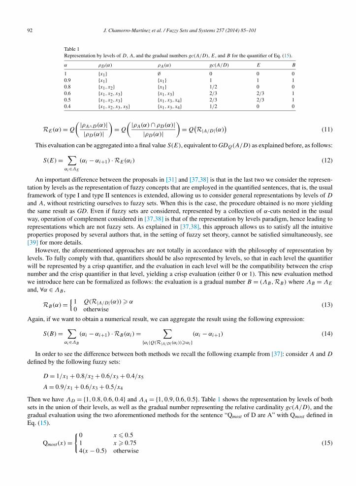
Table 1Representation by levels of D, A, and the gradual numbers gc(A/D), E, and B for the quantifier of Eq. (15).

α ρD(α) ρA(α) gc(A/D) E B

1 {x1} ∅ 0 0 00.9 {x1} {x1} 1 1 10.8 {x1, x2} {x1} 1/2 0 00.6 {x1, x2, x3} {x1, x3} 2/3 2/3 10.5 {x1, x2, x3} {x1, x3, x4} 2/3 2/3 10.4 {x1, x2, x3, x5} {x1, x3, x4} 1/2 0 0

RE(α) = Q

( |ρA∧D(α)||ρD(α)|

)= Q

( |ρA(α) ∩ ρD(α)||ρD(α)|

)= Q

(R|A/D|(α)

)(11)

This evaluation can be aggregated into a final value S(E), equivalent to GDQ(A/D) as explained before, as follows:

S(E) =∑

αi∈ΛE

(αi − αi+1) ·RE(αi) (12)

An important difference between the proposals in [31] and [37,38] is that in the last two we consider the represen-tation by levels as the representation of fuzzy concepts that are employed in the quantified sentences, that is, the usualframework of type I and type II sentences is extended, allowing us to consider general representations by levels of D

and A, without restricting ourselves to fuzzy sets. When this is the case, the procedure obtained is no more yieldingthe same result as GD. Even if fuzzy sets are considered, represented by a collection of α-cuts nested in the usualway, operation of complement considered in [37,38] is that of the representation by levels paradigm, hence leading torepresentations which are not fuzzy sets. As explained in [37,38], this approach allows us to satisfy all the intuitiveproperties proposed by several authors that, in the setting of fuzzy set theory, cannot be satisfied simultaneously, see[39] for more details.

However, the aforementioned approaches are not totally in accordance with the philosophy of representation bylevels. To fully comply with that, quantifiers should be also represented by levels, so that in each level the quantifierwill be represented by a crisp quantifier, and the evaluation in each level will be the compatibility between the crispnumber and the crisp quantifier in that level, yielding a crisp evaluation (either 0 or 1). This new evaluation methodwe introduce here can be formalized as follows: the evaluation is a gradual number B = (ΛB,RB) where ΛB = ΛE

and, ∀α ∈ ΛB ,

RB(α) ={

1 Q(R|A/D|(α)) � α

0 otherwise(13)

Again, if we want to obtain a numerical result, we can aggregate the result using the following expression:

S(B) =∑

αi∈ΛB

(αi − αi+1) ·RB(αi) =∑

{αi |Q(R|A/D|(αi ))�αi }(αi − αi+1) (14)

In order to see the difference between both methods we recall the following example from [37]: consider A and D

defined by the following fuzzy sets:

D = 1/x1 + 0.8/x2 + 0.6/x3 + 0.4/x5

A = 0.9/x1 + 0.6/x3 + 0.5/x4

Then we have ΛD = {1,0.8,0.6,0.4} and ΛA = {1,0.9,0.6,0.5}. Table 1 shows the representation by levels of bothsets in the union of their levels, as well as the gradual number representing the relative cardinality gc(A/D), and thegradual evaluation using the two aforementioned methods for the sentence “Qmost of D are A” with Qmost defined inEq. (15).

Qmost(x) ={0 x � 0.5

1 x � 0.75 (15)

4(x − 0.5) otherwise

J. Chamorro-Martínez et al. / Fuzzy Sets and Systems 257 (2014) 85–101 93

We can see that B provides a crisp evaluation in each level. Finally, using the aggregations previously defined,we have S(E) = 7/15 ≈ 0.46 and S(B) = 0.3. We shall study further properties of the new method in a forthcomingpaper.

4. Some applications in image processing

In this section we show two applications of fuzzy cardinality and quantification in image processing. As we haveconcluded in previous sections, the basic idea is to employ gradual numbers for measuring cardinality when the latteris to be employed in further calculations. On the contrary, when the idea is to provide information to a human userabout the cardinality, the idea is to employ fuzzy quantification in order to calculate the compatibility between thecardinality, measured as a gradual number, and a collection of fuzzy numbers corresponding to linguistic quantifiers,in order to provide the most compatible one to the user. This collection of quantifiers will form the vocabulary that weconsider understandable to the user.

The two applications we show here are related to the cardinality of the fuzzy colors in an image, understood as thecardinality of the fuzzy subset of pixels having that fuzzy color. Hence, we shall start recalling the notion of fuzzycolor space we introduced in [41]. Then we shall describe the application of fuzzy cardinality and quantification inthe calculation of histograms of colors and dominant colors.

4.1. Fuzzy color spaces

In order to represent the semantic compatibility between crisp colors and linguistic color terms, in [41] we intro-duced the following definitions of fuzzy color and fuzzy color space on a generic crisp color space XYZ with domainof components being DX , DY , and DZ :

Definition 4.1. (See [41].) A fuzzy color C̃ is a linguistic label whose semantics is represented in a color space XYZ

by a normalized fuzzy subset of DX × DY × DZ .

Definition 4.2. (See [41].) A fuzzy color space X̃YZ is a set of fuzzy colors C̃1, . . . , C̃m that define a fuzzy partitionof DX × DY × DZ in the sense that it satisfies:

1.⋃m

i=1 sup(C̃i) = XYZ, i.e., the union of the supports of the C̃i covers the whole space.2. ker(C̃i)∩ ker(C̃j ) = ∅ ∀i �= j , i.e., the kernels of the C̃i and C̃j are pairwise disjoint, where ker(C̃) = {c ∈ XYZ |

C̃(c) = 1}.3. ∀i ∈ {1, . . . ,m} ∃c ∈ XYZ such that C̃i(c) = 1, i.e., there is at least one object fully representative of the fuzzy

color C̃i .

Condition 3 is always verified by definition of fuzzy color. Condition 1 implies ∀c ∈ XYZ ∃i ∈ {1, . . . ,m} suchthat C̃i(c) > 0. Conditions 2 and 3 imply C̃i � C̃j ∀i �= j . Notice the usual definition of fuzzy partition given by∑m

i=1 C̃i(c) = 1.In [41] we proposed several fuzzy color spaces using color names provided by the well-known ISCC–NBS sys-

tem [28]. ISCC–NBS provides several color sets in the form of sets of pairs (linguistic term, crisp color). Using themethodology introduced in [41], we calculate for each color set a fuzzy color space on the basis of a Voronoi diagramof the crisp color space, calculated using the crisp colors of the set of pairs considered. The Voronoi diagram is a crisppartition corresponding to the 0.5-cut of the fuzzy colors. The kernel and support of each fuzzy color are obtained asa scaling with parameters α and β respectively, with α < 1 < β , and guaranteeing the conditions in Definition 4.2.The membership functions of the fuzzy colors are obtained on the basis of distances in the crisp color space. For moredetails see [41].

In [41], we have obtained three fuzzy color spaces on the basis of the sets of color names Basic (13 colors),Extended (31 colors) and Complete (267 colors) in the RGB color space. For instance, the Basic set has color namescorresponding to ten basic color terms (pink, red, orange, yellow, brown, olive, green, blue, violet, purple), and 3achromatic ones (white, gray, and black). The corresponding representative crisp colors are shown in Fig. 1, togetherwith a rough view of the core, the α-cuts of level 0.5, and the support of some fuzzy colors in the fuzzy color space

94 J. Chamorro-Martínez et al. / Fuzzy Sets and Systems 257 (2014) 85–101

Fig. 1. Part of the RGB fuzzy color space obtained in [41] from the ISCC–NBS Basic set of colors. (a) ISCC–NBS Basic set of colors (representativecrisp color and color name). (b) Situation of the representative crisp colors in the RGB color space. (c) Volumes of colors in the 0.5-cut for thefuzzy colors yellow, blue, green, and gray obtained from the Voronoi diagram in the RGB cube. (d) Volumes of colors in the kernel of the samefuzzy colors. (e) Volume of colors in the support of the fuzzy color yellow. (f) Superimposed views of part of the surfaces of the volumes of colorsin the kernel (most internal), 0.5-cut (middle) and support (most external) for the fuzzy color yellow. (For interpretation of the references to colorin this figure, the reader is referred to the web version of this article.)

obtained from ISCC–NBS Basic in [41]. We are not showing examples of the fuzzy color spaces for the sets Extendedand Complete because of the lack of space.

4.2. Histograms on fuzzy color spaces

Histograms are the basis of many techniques for image restoration, enhancement, segmentation, retrieval, etc. Inprinciple, a color histogram is defined as a function h(ck) = nk where ck = [x, y, z] is a color and nk is the number ofpixels in the image having the color ck. It is common to normalize a histogram by dividing each of its values by thetotal number of pixels, obtaining the frequency of occurrence of a color ck.

This simple approach has the drawback that a crisp color space is not representative of the collection of colorswe can distinguish and identify. In addition, the values nk are to be very low because there are many colors in acrisp color space, and it is easy to find small color variations in real images. Since in practice many of the colors ckare indistinguishable for us, a solution is to use an histogram defined on groups of indistinguishable colors Ck , inwhich the associated number of pixels is h(Ck) = ∑

ck∈CKnk . The collection of groups of colors C1, . . . ,Cn defines

a partition (quantization) of the color space employed.For this purpose, we shall employ the fuzzy color spaces introduced in the previous section. This approach has the

advantage that it is able to represent the fact that indistinguishability is a fuzzy, gradual concept for us, i.e., colorsare indistinguishable to a certain degree. Crisp boundaries inherent to crisp quantization are counterintuitive for us. Inaddition, both the (fuzzy) quantization and the histograms are less sensitive to small variations of the boundaries.

In the literature there are several proposals which define histograms over a set of fuzzy colors [18,26,34,35]. Onedrawback of most of these proposals is that they work only with intensities.

In [10] we employed non-convex fuzzy subsets of the non-negative integers for defining fuzzy histograms. Thisapproach represents a compromise between the advantages and disadvantages of using fuzzy numbers and gradual

J. Chamorro-Martínez et al. / Fuzzy Sets and Systems 257 (2014) 85–101 95

numbers. In [11] we proposed two kinds of color histograms: one based on gradual numbers, to be used in practiceby the computer for image processing, and an approximation of this histogram by means of linguistic labels (fuzzynumbers) in order to give information to the user. These are introduced and illustrated in the next sections.

4.2.1. Gradual histogramDefinition 4.3. A gradual color histogram is a function hG that assigns a gradual number to every fuzzy color in afuzzy color space X̃YZ.

The gradual number corresponding to every fuzzy color C̃ is obtained by assigning to α the cardinality of the α-cutof the fuzzy subset of pixels with color C̃. Since the fuzzy subset of pixels with color C̃ is finite, in practice we needonly a finite number of cuts for representing the gradual number. However, this number may be large, so in somecases it may be interesting to consider just a fixed collection of cuts with equidistant values of α. See [36] for furtherdiscussion on that.

Let us remark that the gradual integer number can be easily transformed into a gradual rational number by dividingthe number associated to each level α by the total number of pixels in the image. This is convenient when we wantthe histogram to represent proportions instead of absolute values. We shall see examples in Section 4.2.3.

Finally, usual image processing operations performed on crisp histograms can be extended directly to gradualhistograms by using Definition 2.1, i.e., by applying the operation in each level.

4.2.2. Linguistic histogramLet X̃YZ be a fuzzy color space. Let us consider a collection of fuzzy linguistic quantifiers SQ = {Q1, . . . ,Qk}

provided by the user, like Around 10% or Most, represented by appropriate fuzzy subsets of the unit interval, andBetween 50 and 100, represented by appropriate fuzzy subsets of the non-negative integers.

Definition 4.4. A linguistic color histogram is a function hL that assigns a linguistic quantifier from SQ to every fuzzy

color in X̃YZ.

We consider user-defined quantifiers in order to improve understandability, since accuracy of the linguistic ap-proach is always worse than that of the gradual approach.

In order to obtain the quantifier for every fuzzy color C̃, we take the gradual number associated to C̃ in the gradualcolor histogram (an accurate representation of cardinality) and we calculate the compatibility between this gradualnumber and every quantifier in SQ. The quantifier that yields maximum compatibility is then chosen to represent thelinguistic amount or proportion of pixels having color in the linguistic histogram. The compatibility is calculated byevaluating the accomplishment degree of the quantified statement Qi of pixels in the image are painted in C̃, usingone suitable evaluation method. In this paper we shall consider the method we have introduced in Section 3.3.

4.2.3. A first synthetic exampleOur first example, taken from [36], allows us to illustrate the differences between the different approaches to

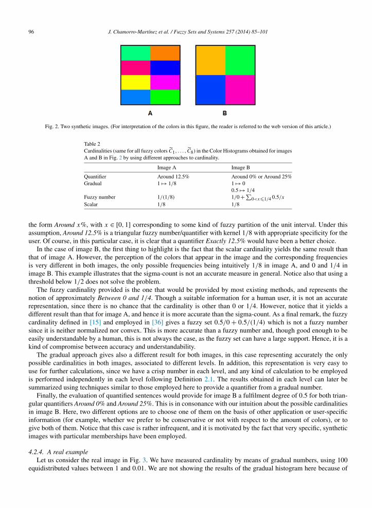
cardinality of fuzzy sets discussed in Section 2. The fuzzy color space employed here, described in [36], is not thatof Section 4.1, but this is unimportant for our purpose in this first example. Fig. 2 shows two images, the first onecontaining eight crisp colors in the kernel of different fuzzy colors. Let C̃1, . . . , C̃8 denote these colors, from left toright and top to bottom (see [36] for a definition of the membership functions). In the second one we have four crispcolors that are compatible to a degree 0.5 with two of the eight fuzzy colors in the first image.

Table 2 shows the (relative) cardinality of the fuzzy set of pixels painted in each fuzzy color in both images,using different approaches. The result is the same for all the fuzzy colors in both images by the way they have beendefined. In the case of image A, since the eight crisp colors employed are in the kernel of fuzzy colors, the sets ofpixels painted in every fuzzy color are crisp, and hence a crisp cardinality is obtained. In particular, the fuzzy numberfor image A is the same despite the method employed for calculating it. In the gradual approach, crisp results arerepresented by the fact that only the level α = 1 is necessary, since all the levels are assigned the same cardinality(in this case, 1/8). In the case of the quantifier, any quantifier having 1/8 in its core will give a result of 1 in theevaluation of the quantified sentence. We assume here that the user has predefined a collection of quantifiers of

96 J. Chamorro-Martínez et al. / Fuzzy Sets and Systems 257 (2014) 85–101

Fig. 2. Two synthetic images. (For interpretation of the colors in this figure, the reader is referred to the web version of this article.)

Table 2Cardinalities (same for all fuzzy colors C̃1, . . . , C̃8) in the Color Histograms obtained for imagesA and B in Fig. 2 by using different approaches to cardinality.

Image A Image B

Quantifier Around 12.5% Around 0% or Around 25%Gradual 1 �→ 1/8 1 �→ 0

0.5 �→ 1/4Fuzzy number 1/(1/8) 1/0 + ∑

0<x�1/4 0.5/x

Scalar 1/8 1/8

the form Around x%, with x ∈ [0,1] corresponding to some kind of fuzzy partition of the unit interval. Under thisassumption, Around 12.5% is a triangular fuzzy number/quantifier with kernel 1/8 with appropriate specificity for theuser. Of course, in this particular case, it is clear that a quantifier Exactly 12.5% would have been a better choice.

In the case of image B, the first thing to highlight is the fact that the scalar cardinality yields the same result thanthat of image A. However, the perception of the colors that appear in the image and the corresponding frequenciesis very different in both images, the only possible frequencies being intuitively 1/8 in image A, and 0 and 1/4 inimage B. This example illustrates that the sigma-count is not an accurate measure in general. Notice also that using athreshold below 1/2 does not solve the problem.

The fuzzy cardinality provided is the one that would be provided by most existing methods, and represents thenotion of approximately Between 0 and 1/4. Though a suitable information for a human user, it is not an accuraterepresentation, since there is no chance that the cardinality is other than 0 or 1/4. However, notice that it yields adifferent result than that for image A, and hence it is more accurate than the sigma-count. As a final remark, the fuzzycardinality defined in [15] and employed in [36] gives a fuzzy set 0.5/0 + 0.5/(1/4) which is not a fuzzy numbersince it is neither normalized nor convex. This is more accurate than a fuzzy number and, though good enough to beeasily understandable by a human, this is not always the case, as the fuzzy set can have a large support. Hence, it is akind of compromise between accuracy and understandability.

The gradual approach gives also a different result for both images, in this case representing accurately the onlypossible cardinalities in both images, associated to different levels. In addition, this representation is very easy touse for further calculations, since we have a crisp number in each level, and any kind of calculation to be employedis performed independently in each level following Definition 2.1. The results obtained in each level can later besummarized using techniques similar to those employed here to provide a quantifier from a gradual number.

Finally, the evaluation of quantified sentences would provide for image B a fulfilment degree of 0.5 for both trian-gular quantifiers Around 0% and Around 25%. This is in consonance with our intuition about the possible cardinalitiesin image B. Here, two different options are to choose one of them on the basis of other application or user-specificinformation (for example, whether we prefer to be conservative or not with respect to the amount of colors), or togive both of them. Notice that this case is rather infrequent, and it is motivated by the fact that very specific, syntheticimages with particular memberships have been employed.

4.2.4. A real exampleLet us consider the real image in Fig. 3. We have measured cardinality by means of gradual numbers, using 100

equidistributed values between 1 and 0.01. We are not showing the results of the gradual histogram here because of

J. Chamorro-Martínez et al. / Fuzzy Sets and Systems 257 (2014) 85–101 97

Fig. 3. Real image.

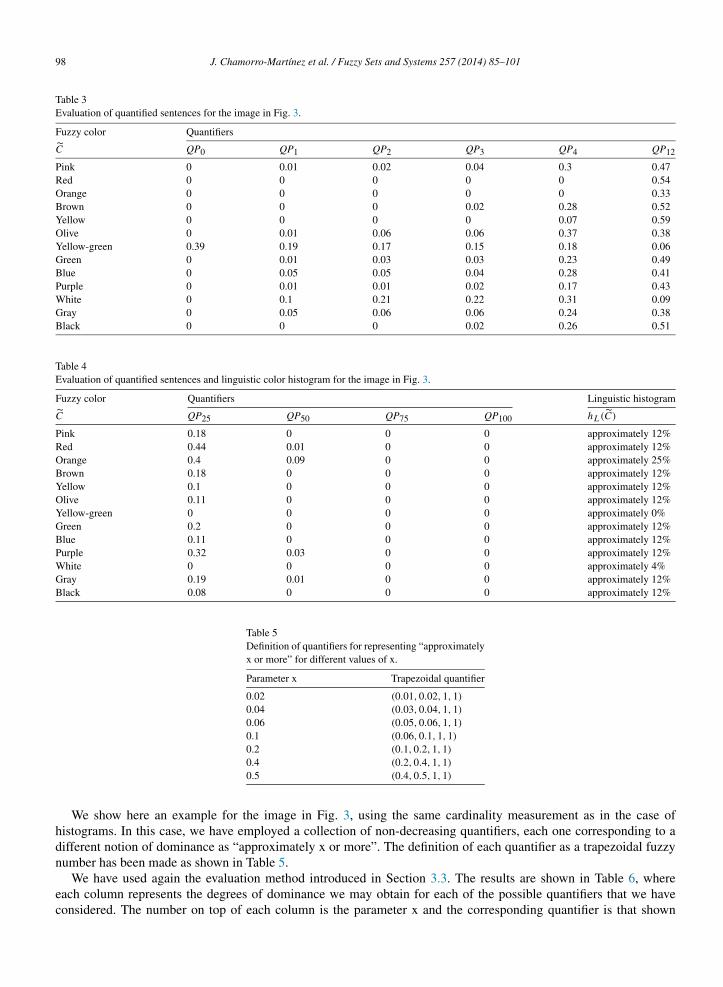
lack of space, being also little informative in a real case to the user. In order to obtain a linguistic histogram, we haveconsidered a collection of ten triangular relative quantifiers defining a fuzzy partition in Ruspini’s sense, with kernelsbeing the percentages 0, 1, 2, 3, 4, 12, 25, 50, 75, and 100. Let us denote by QPx the quantifier with kernel x. Tables 3and 4 show the values obtained by evaluation of the quantified sentences QPx of the pixels are painted in color C̃ forevery fuzzy color C̃ in the fuzzy color space associated to the ISCC–NBS Basic set of colors explained in Section 4.1.We have employed the new method introduced in Section 3.3 for evaluating the sentence, obtaining the compatibilitybetween the gradual number measuring the cardinality, and the quantifier. The last column in Table 4 contains thevalues of the linguistic histogram.

Let us remark that the addition of the result of the evaluation of quantified sentences is not necessarily 1, sincethese are not frequencies but values of compatibility between cardinality and quantifiers. Similarly, the addition ofthe quantities indicated in the linguistic histogram is not expected to be 100% in general, since these are fuzzy setsaround the value. Specificity also plays a role here, for example, the collection of quantifiers employed here “jump”from 4% to 12%, hence the latter quantifier is much less specific than those between 0–4%. In practice, we are justworking on the basis of the quantifiers the user is interested in, his/her vocabulary, and the results may vary dependingon the number and definition of quantifiers, and the fuzzy color space employed. However, we think that the resultsare compatible with what we can see in the image. Finally, choosing more than one quantifier when the differencein the accomplishment degree is very low can be an interesting alternative in some cases, particularly when there areseveral quantifiers with a compatibility degree close to the maximum.

4.3. Color dominance

Color dominance is an important concept in image processing. The dominant color descriptor is one of the mostimportant descriptors in MPEG-7. The notion of dominance is basically related to the frequency of the color in theimage, though other aspects may be also taken into account. A dominant color descriptor must provide an effective,compact, and intuitive representation of the most representative (frequent) colors present in an image.

Many approaches to dominant color extraction have been proposed in the literature [50,30]. Most of them performthe extraction process based on histogram analysis [42,53] or clustering techniques [29] in color domain. Nevertheless,these approaches consider a crisp notion of dominance, when in fact for human’s perception there are degrees ofdominance, that is, colors can be clearly dominant, clearly not dominant, or can be dominant to a certain degree. Inaddition, most of the times they do not consider subsets of crisp colors, as represented in computers, that fully matchhuman perception as expressed by linguistic color terms.

We have proposed to define the fuzzy concept dominant via quantifiers in previous works [9,8,12]. A fuzzy non-decreasing quantifier is a natural way to represent the semantics of the concept on the basis of the amount of pixelshaving a certain color.

98 J. Chamorro-Martínez et al. / Fuzzy Sets and Systems 257 (2014) 85–101

Table 3Evaluation of quantified sentences for the image in Fig. 3.

Fuzzy color Quantifiers

C̃ QP0 QP1 QP2 QP3 QP4 QP12

Pink 0 0.01 0.02 0.04 0.3 0.47Red 0 0 0 0 0 0.54Orange 0 0 0 0 0 0.33Brown 0 0 0 0.02 0.28 0.52Yellow 0 0 0 0 0.07 0.59Olive 0 0.01 0.06 0.06 0.37 0.38Yellow-green 0.39 0.19 0.17 0.15 0.18 0.06Green 0 0.01 0.03 0.03 0.23 0.49Blue 0 0.05 0.05 0.04 0.28 0.41Purple 0 0.01 0.01 0.02 0.17 0.43White 0 0.1 0.21 0.22 0.31 0.09Gray 0 0.05 0.06 0.06 0.24 0.38Black 0 0 0 0.02 0.26 0.51

Table 4Evaluation of quantified sentences and linguistic color histogram for the image in Fig. 3.

Fuzzy color Quantifiers Linguistic histogram

C̃ QP25 QP50 QP75 QP100 hL(C̃)

Pink 0.18 0 0 0 approximately 12%Red 0.44 0.01 0 0 approximately 12%Orange 0.4 0.09 0 0 approximately 25%Brown 0.18 0 0 0 approximately 12%Yellow 0.1 0 0 0 approximately 12%Olive 0.11 0 0 0 approximately 12%Yellow-green 0 0 0 0 approximately 0%Green 0.2 0 0 0 approximately 12%Blue 0.11 0 0 0 approximately 12%Purple 0.32 0.03 0 0 approximately 12%White 0 0 0 0 approximately 4%Gray 0.19 0.01 0 0 approximately 12%Black 0.08 0 0 0 approximately 12%

Table 5Definition of quantifiers for representing “approximatelyx or more” for different values of x.

Parameter x Trapezoidal quantifier

0.02 (0.01,0.02,1,1)

0.04 (0.03,0.04,1,1)

0.06 (0.05,0.06,1,1)

0.1 (0.06,0.1,1,1)

0.2 (0.1,0.2,1,1)

0.4 (0.2,0.4,1,1)

0.5 (0.4,0.5,1,1)

We show here an example for the image in Fig. 3, using the same cardinality measurement as in the case ofhistograms. In this case, we have employed a collection of non-decreasing quantifiers, each one corresponding to adifferent notion of dominance as “approximately x or more”. The definition of each quantifier as a trapezoidal fuzzynumber has been made as shown in Table 5.

We have used again the evaluation method introduced in Section 3.3. The results are shown in Table 6, whereeach column represents the degrees of dominance we may obtain for each of the possible quantifiers that we haveconsidered. The number on top of each column is the parameter x and the corresponding quantifier is that shown

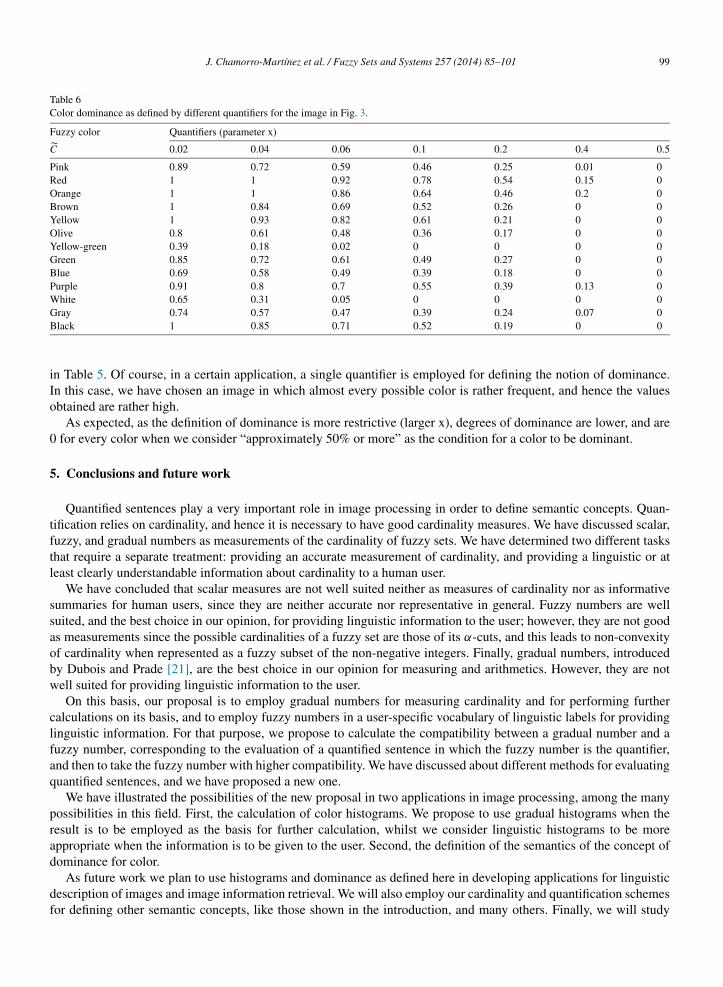
J. Chamorro-Martínez et al. / Fuzzy Sets and Systems 257 (2014) 85–101 99

Table 6Color dominance as defined by different quantifiers for the image in Fig. 3.

Fuzzy color Quantifiers (parameter x)

C̃ 0.02 0.04 0.06 0.1 0.2 0.4 0.5

Pink 0.89 0.72 0.59 0.46 0.25 0.01 0Red 1 1 0.92 0.78 0.54 0.15 0Orange 1 1 0.86 0.64 0.46 0.2 0Brown 1 0.84 0.69 0.52 0.26 0 0Yellow 1 0.93 0.82 0.61 0.21 0 0Olive 0.8 0.61 0.48 0.36 0.17 0 0Yellow-green 0.39 0.18 0.02 0 0 0 0Green 0.85 0.72 0.61 0.49 0.27 0 0Blue 0.69 0.58 0.49 0.39 0.18 0 0Purple 0.91 0.8 0.7 0.55 0.39 0.13 0White 0.65 0.31 0.05 0 0 0 0Gray 0.74 0.57 0.47 0.39 0.24 0.07 0Black 1 0.85 0.71 0.52 0.19 0 0

in Table 5. Of course, in a certain application, a single quantifier is employed for defining the notion of dominance.In this case, we have chosen an image in which almost every possible color is rather frequent, and hence the valuesobtained are rather high.

As expected, as the definition of dominance is more restrictive (larger x), degrees of dominance are lower, and are0 for every color when we consider “approximately 50% or more” as the condition for a color to be dominant.

5. Conclusions and future work

Quantified sentences play a very important role in image processing in order to define semantic concepts. Quan-tification relies on cardinality, and hence it is necessary to have good cardinality measures. We have discussed scalar,fuzzy, and gradual numbers as measurements of the cardinality of fuzzy sets. We have determined two different tasksthat require a separate treatment: providing an accurate measurement of cardinality, and providing a linguistic or atleast clearly understandable information about cardinality to a human user.

We have concluded that scalar measures are not well suited neither as measures of cardinality nor as informativesummaries for human users, since they are neither accurate nor representative in general. Fuzzy numbers are wellsuited, and the best choice in our opinion, for providing linguistic information to the user; however, they are not goodas measurements since the possible cardinalities of a fuzzy set are those of its α-cuts, and this leads to non-convexityof cardinality when represented as a fuzzy subset of the non-negative integers. Finally, gradual numbers, introducedby Dubois and Prade [21], are the best choice in our opinion for measuring and arithmetics. However, they are notwell suited for providing linguistic information to the user.

On this basis, our proposal is to employ gradual numbers for measuring cardinality and for performing furthercalculations on its basis, and to employ fuzzy numbers in a user-specific vocabulary of linguistic labels for providinglinguistic information. For that purpose, we propose to calculate the compatibility between a gradual number and afuzzy number, corresponding to the evaluation of a quantified sentence in which the fuzzy number is the quantifier,and then to take the fuzzy number with higher compatibility. We have discussed about different methods for evaluatingquantified sentences, and we have proposed a new one.

We have illustrated the possibilities of the new proposal in two applications in image processing, among the manypossibilities in this field. First, the calculation of color histograms. We propose to use gradual histograms when theresult is to be employed as the basis for further calculation, whilst we consider linguistic histograms to be moreappropriate when the information is to be given to the user. Second, the definition of the semantics of the concept ofdominance for color.

As future work we plan to use histograms and dominance as defined here in developing applications for linguisticdescription of images and image information retrieval. We will also employ our cardinality and quantification schemesfor defining other semantic concepts, like those shown in the introduction, and many others. Finally, we will study

100 J. Chamorro-Martínez et al. / Fuzzy Sets and Systems 257 (2014) 85–101

further properties of the quantification method introduced here in the framework of the representation by levels ofconcepts with fuzziness.

Acknowledgement

This work has been partially supported by the Spanish Government under project TIN2009-08296.

References

[1] S. Barro, A. Bugarín, P. Cariñena, F. Díaz-Hermida, A framework for fuzzy quantification models analysis, IEEE Trans. Fuzzy Syst. 11 (1)(2003) 89–99.

[2] S. Barro, A. Bugarín, P. Cariñena, F. Díaz-Hermida, Voting-model based evaluation of fuzzy quantified sentences: A general framework,Fuzzy Sets Syst. 146 (1) (2004) 97–120.

[3] J. Barwise, R. Cooper, Generalized quantifiers and natural language, Linguist. Philos. 4 (1981) 159–219.[4] I. Blanco, M. Delgado, M.J. Martín-Bautista, D. Sánchez, M.A. Vila, Quantifier guided aggregation of fuzzy criteria with associated impor-

tances, in: T. Calvo, R. Mesiar, G. Mayor (Eds.), Aggregation Operators. New Trends and Applications, in: Studies in Fuzziness and SoftComputing Series, Physica-Verlag, 2002, pp. 272–287.

[5] P. Bosc, L. Lietard, Monotonic quantified statements and fuzzy integrals, in: Proc. NAFIPS/IFIS/NASA Conference, 1994, pp. 8–12.[6] P. Bosc, L. Lietard, On the comparison of the Sugeno and the Choquet fuzzy integrals for the evaluation of quantified statements, in: Proc. of

EUFIT’95, 1995, pp. 709–716.[7] J. Casasnovas, J. Torrens, Scalar cardinalities of finite fuzzy sets for t-norms and t-conorms, Int. J. Uncertain. Fuzziness Knowl.-Based Syst.

11 (5) (2003) 599–614.[8] J. Chamorro-Martínez, P. Martínez-Jiménez, J.M. Soto-Hidalgo, A fuzzy approach for retrieving images in databases using dominant color

and texture descriptors, in: Proceedings IEEE WCCI 2010, 2010, pp. 88–94.[9] J. Chamorro-Martínez, J.M. Medina, C. Barranco, E. Galán-Perales, J.M. Soto-Hidalgo, Retrieving images in fuzzy object-relational databases

using dominant color descriptors, Fuzzy Sets Syst. 158 (3) (2007) 312–324.[10] J. Chamorro-Martínez, D. Sánchez, J.M. Soto-Hidalgo, A novel histogram definition for fuzzy color spaces, in: Proceedings IEEE WCCI

2008, 2008, pp. 2149–2156.[11] J. Chamorro-Martínez, D. Sánchez, J.M. Soto-Hidalgo, P. Martínez-Jiménez, Histograms for fuzzy color spaces, in: P. Melo-Pinto, P. Couto,

C. Serodio, J. Fodor, B. de Baets (Eds.), EUROFUSE 2011, in: Advances in Intelligent and Soft Computing, vol. 107, Springer, 2011,pp. 339–350.

[12] J. Chamorro-Martínez, J.M. Soto-Hidalgo, D. Sánchez, P. Martínez-Jiménez, An approach for fuzzy dominant color descriptor, in: IFSA 2011,2011.

[13] J.C. Cubero, J.M. Medina, O. Pons, M.A. Vila, Using OWA operator in flexible query processing, in: R.R. Yager, J. Kacprzyk (Eds.), TheOrdered Weighted Averaging Operators: Theory, Methodology and Applications, Kluwer Academic Publishers, 1997, pp. 258–274.

[14] L. Cui, Y. Li, Linguistic quantifiers based on Choquet integrals, Int. J. Approx. Reason. 48 (2008) 559–582.[15] M. Delgado, M.J. Martín-Bautista, D. Sánchez, M.A. Vila, A probabilistic definition of a nonconvex fuzzy cardinality, Fuzzy Sets Syst. 126 (2)

(2002) 41–54.[16] M. Delgado, D. Sánchez, M.A. Vila, Fuzzy cardinality based evaluation of quantified sentences, Int. J. Approx. Reason. 23 (2000) 23–66.[17] F. Díaz-Hermida, A. Bugarín, S. Barro, Definition and classification of semi-fuzzy quantifiers for the evaluation of fuzzy quantified sentences,

Int. J. Approx. Reason. 34 (2003) 49–88.[18] A. Doulamis, N. Doulamis, Fuzzy histograms for efficient visual content representation: Application to content-based image retrieval, in:

IEEE International Conference on Multimedia and Expo, Aug 2001, pp. 893–896.[19] D. Dubois, H. Prade, Fuzzy cardinality and the modeling of imprecise quantification, Fuzzy Sets Syst. 16 (1985) 199–230.[20] D. Dubois, H. Prade, Fuzzy intervals versus fuzzy numbers: Is there a missing concept in fuzzy set theory?, in: Linz Seminar 2005 Abstracts,

2005, pp. 45–46.[21] D. Dubois, H. Prade, Gradual elements in a fuzzy set, Soft Comput. 12 (2008) 165–175.[22] I. Glöckner, DFS – An Axiomatic Approach to Fuzzy Quantification, Technical Report TR97-06, Technical Faculty, University Bielefeld,

Bielefeld, Germany, 1997.[23] I. Glöckner, Fundamentals of Fuzzy Quantification, Technical Report TR2002-07, Technical Faculty, University Bielefeld, Bielefeld, Germany,

2002.[24] I. Glöckner, Evaluation of quantified propositions in generalized models of fuzzy quantification, Int. J. Approx. Reason. 37 (2004) 93–126.[25] I. Glöckner, Generalized fuzzy quantifiers and the modeling of fuzzy branching quantification, Int. J. Intell. Syst. 24 (2009) 624–648.[26] J. Han, K.-K. Ma, Fuzzy color histogram and its use in color image retrieval, IEEE Trans. Image Process. 11 (8) (2002) 944–952.[27] E.L. Keenan, D. Westerståhl, Generalized quantifiers in linguistics and logic, in: J.V. Benthem, A.T. Meulen (Eds.), Handbook of Logic and

Language, Elsevier, 1997, pp. 837–893 (Chapter 15).[28] K.L. Kelly, D.B. Judd, Color: Universal Language and Dictionary of Names, Natl. Bur. Stand. (USA), vol. 440, 1976.[29] S. Kiranyaz, S. Uhlmann, M. Gabbouj, Dominant color extraction based on dynamic clustering by multi-dimensional particle swarm opti-

mization, in: Seventh International Workshop on Content-Based Multimedia Indexing, 2009, CBMI ’09, 2009, pp. 181–188.[30] A. Li, X. Bao, Extracting image dominant color features based on region growing, in: International Conference on Web Information Systems

and Mining (WISM), 2010, 2010, pp. 120–123.

J. Chamorro-Martínez et al. / Fuzzy Sets and Systems 257 (2014) 85–101 101

[31] L. Lietard, D. Rocacher, Evaluation of quantified statements using gradual numbers, in: J. Galindo (Ed.), Handbook of Research on FuzzyInformation Processing in Databases, Information Science Reference, Hershey, PA, USA, 2008, pp. 246–269.

[32] A. De Luca, S. Termini, A definition of a nonprobabilistic entropy in the setting of fuzzy sets theory, Inf. Control 20 (1972) 301–312.[33] D. Ralescu, Cardinality, quantifiers and the aggregation of fuzzy criteria, Fuzzy Sets Syst. 69 (1995) 355–365.[34] S. Romani, P. Sobrevilla, E. Montseny, Obtaining the relevant colors of an image through stability-based fuzzy color histograms, in: IEEE

International Conference on Fuzzy Systems, vol. 2, St. Louis, MI, USA, May 2003, pp. 914–919.[35] T.A. Runkler, Fuzzy histograms and fuzzy chi-squared tests for independence, in: IEEE International Conference on Fuzzy Systems, vol. 3,

July 2004, pp. 1361–1366.[36] D. Sánchez, M. Delgado, M.A. Vila, RL-numbers: An alternative to fuzzy numbers for the representation of imprecise quantities, in: Proc.

Fuzz-IEEE 2008, 2008, pp. 2058–2065.[37] D. Sánchez, M. Delgado, M.A. Vila, Fuzzy quantification using restriction levels, in: Proc. WILF 2009, in: LNCS, vol. 5571, Springer, 2009,

pp. 28–35.[38] D. Sánchez, M. Delgado, M.A. Vila, An approach to general quantification using representation by levels, in: Proc. WILF 2011, in: LNAI,

vol. 6857, Springer, 2011, pp. 50–57.[39] D. Sánchez, M. Delgado, M.A. Vila, J. Chamorro-Martínez, Evaluation of fuzzy quantified sentences: Keeping the boolean properties, in:

Proceedings of NAFIPS 2012, 2012, pp. 76–81.[40] D. Sánchez, M. Delgado, M.A. Vila, J. Chamorro-Martínez, On a non-nested level-based representation of fuzziness, Fuzzy Sets Syst. 192

(2012) 159–175.[41] J.M. Soto-Hidalgo, J. Chamorro-Martínez, D. Sánchez, A new approach for defining a fuzzy color space, in: Proceedings IEEE WCCI 2010,

2010, pp. 292–297.[42] K.M. Wong, C.H. Chey, T.S. Liu, L.M. Po, Dominant color image retrieval using merged histogram, in: Proceedings of the 2003 International

Symposium on Circuits and Systems, ISCAS ’03, 2003, pp. 908–911.[43] M. Wygralak, Vaguely Defined Objects. Representations, Fuzzy Sets and Nonclassical Cardinality Theory, Kluwer Academic Press, Dor-

drecht/Boston/London, 1996.[44] M. Wygralak, On the best scalar approximation of cardinality of a fuzzy set, Int. J. Uncertain. Fuzziness Knowl.-Based Syst. 5 (6) (1997)

681–687.[45] M. Wygralak, Questions of cardinality of finite fuzzy sets, Fuzzy Sets Syst. 102 (6) (1999) 185–210.[46] M. Wygralak, An axiomatic approach to scalar cardinalities of fuzzy sets, Fuzzy Sets Syst. 110 (2000) 175–179.[47] M. Wygralak, Cardinalities of Fuzzy Sets, Springer, 2003.[48] R.R. Yager, General multiple-objective decision functions and linguistically quantified statements, Int. J. Man-Mach. Stud. 21 (1984) 389–400.[49] R.R. Yager, On ordered weighted averaging aggregation operators in multicriteria decisionmaking, IEEE Trans. Syst. Man Cybern. 18 (1)

(1988) 183–190.[50] Nai-Chung Yang, Wei-Han Chang, Chung-Ming Kuo, Tsia-Hsing Li, A fast mpeg-7 dominant color extraction with new similarity measure

for image retrieval, J. Vis. Commun. Image Represent. 19 (2) (2008) 92–105.[51] M. Ying, On Zadeh’s method for interpreting linguistically quantified proposition, in: Proceedings of the 18th IEEE Int. Symp. on Multiple-

Valued Logic, 1988, pp. 248–252.[52] M. Ying, Linguistic quantifiers modeled by Sugeno integrals, Artif. Intell. 170 (2006) 581–606.[53] S.S. Yu, S.Y. Huang, Y.H. Pan, H.C. Wu, An easy dominant color extraction and edge valley histogram for image retrieval, in: 2010 Interna-

tional Computer Symposium (ICS), 2010, pp. 159–164.[54] L.A. Zadeh, A theory of approximate reasoning, Mach. Intell. 9 (1979) 149–194.[55] L.A. Zadeh, A computational approach to fuzzy quantifiers in natural languages, Comput. Math. Appl. 9 (1) (1983) 149–184.