perspective shape from shading: ambiguity analysis and ... · perspective shape from shading:...

SIAM J. IMAGING SCIENCES c© 2012 Society for Industrial and Applied MathematicsVol. 5, No. 1, pp. 311–342

Perspective Shape from Shading: Ambiguity Analysisand Numerical Approximations∗

Michael Breuß†, Emiliano Cristiani‡, Jean-Denis Durou§, Maurizio Falcone¶, and Oliver Vogel†

Abstract. In this paper we study a perspective model for shape from shading and its numerical approxima-tion. We show that an ambiguity still persists, although the model with light attenuation factor haspreviously been shown to be well-posed under appropriate assumptions. Analytical results revealingthe ambiguity are complemented by various numerical tests. Moreover, we present convergence re-sults for two iterative approximation schemes. The first is based on a finite difference discretization,whereas the second is based on a semi-Lagrangian discretization. The convergence results are ob-tained in the general framework of viscosity solutions of the underlying partial differential equation.In addition to these theoretical and numerical results, we propose an algorithm for reconstructingdiscontinuous surfaces, making it possible to obtain results of reasonable quality even for complexscenes. To this end, we solve the constituting equation on a previously segmented input image,using state constraint boundary conditions at the segment borders.

Key words. shape from shading, ambiguity analysis, Hamilton–Jacobi equations, finite difference methods,semi-Lagrangian schemes

AMS subject classifications. 68U10, 35A02, 65N06, 65N12, 65N20, 65N21

DOI. 10.1137/100815104

1. Introduction. The shape from shading (SFS) problem amounts to the reconstructionof the three-dimensional (3-D) structure of objects given a single two-dimensional (2-D) grayvalue image of them. For this task, the SFS process relies on information on the illuminationand the light reflectance in the scene. It was introduced by Horn [20] and is a classic inverseproblem in computer vision with many potential applications; see, e.g., [16, 21, 22, 38] andthe references therein for an overview.

In this paper we deal with a perspective SFS model as proposed in [25, 31, 34], takinginto account the so-called light attenuation factor; cf. [31]. This SFS model has gained someattention in the recent literature. It combines desirable theoretical properties with a reasonablequality of results compared to other approaches in SFS. One of its good theoretical properties

∗Received by the editors November 16, 2010; accepted for publication (in revised form) November 26, 2011;published electronically March 8, 2012. This work was partially supported by the PRIN 2007 Project “Metodologieper il calcolo scientifico ed applicazioni avanzate” and by the Deutsche Forschungsgemeinschaft (DFG).

http://www.siam.org/journals/siims/5-1/81510.html†Faculty of Mathematics and Computer Science, Saarland University, Building E1.1, 66041 Saarbrucken, Germany

([email protected], [email protected]).‡Dipartimento di Matematica, SAPIENZA Universita di Roma, P.le Aldo Moro 2, 00185 Rome, Italy

([email protected]).§Institut de Recherche en Informatique de Toulouse, Universite Paul Sabatier, 118 route de Narbonne, 31062

Toulouse Cedex 9, France, and Centre de Mathematiques et de Leurs Applications, Ecole Normale Superieure deCachan, 61 avenue du president Wilson, 94235 Cachan Cedex, France ([email protected]).

¶Corresponding author. Dipartimento di Matematica, SAPIENZA Universita di Roma, P.le Aldo Moro 2, 00185Rome, Italy ([email protected]).

311

http://www.siam.org/journals/siims/5-1/81510.html

mailto:[email protected]





312 BREUß, CRISTIANI, DUROU, FALCONE, AND VOGEL

is the well-posedness, given some assumptions. However, the question arises whether allthe ambiguities (including the notorious concave/convex ambiguity [20]) have been entirelyvanquished by using the perspective SFS model. For the case that the answer is negative, itwould be of interest to determine whether there is a way to avoid ambiguities. Concerningthe numerical realization of the model, a number of iterative solvers have been proposed andcompared [6]. However, the mathematical validation of some of them is still lacking.

In this paper we address these open issues. By a thorough investigation, we show thatambiguities still arise and appear in practical computations. We propose a way of overcomingthose ambiguities whenever they are caused only by the discontinuity of the surface to bereconstructed. We do this by making use of a segmentation step combined with suitableboundary conditions at the segment borders. In this way, shapes in relatively complex scenesalso can be reconstructed. Moreover, we prove that the two fastest and easiest-to-implementiterative solvers selected in the comparative paper [6] converge to the viscosity solution of theconsidered equation.

Models and ambiguities. Perspective SFS models are distinguished by the assumption thatthe camera performs a perspective projection of the 3-D world to the given 2-D image. Re-cently, a number of perspective SFS models have been considered [11, 29, 34], with promisingapplications to face reconstruction [29], reconstruction of organs [34, 35], and digitization ofdocuments [11, 12].

Within the class of perspective SFS models, that of Okatani and Deguchi [25] is distin-guished by the lighting model. This consists of a point light source located at the opticalcenter combined with a light attenuation term. Okatani and Deguchi proposed a methodfor resolving their model which is an extension of the level set method designed by Kimmelet al. [23] for solving the classic SFS problem. They claimed that their method could bederived from a partial differential equation (PDE) of the form H(x, y, r, rx, ry) = 0, where ris the distance to the point light source, but did not explicitly state it. Prados, Faugeras, andCamilli stated in [32] the first PDE derived from this model, which we now call the PSFSmodel (“P” for “perspective”). A number of papers by Prados and his coauthors have dealtwith its theoretical basis; cf. [27, 28, 30, 31]. Especially, the PSFS model has been shown tobe well-posed under mild assumptions.

The well-posedness of SFS models has been a point of continuous interest in computervision research. This began with Horn [20] who mentions the concave/convex ambiguity in hisclassic orthographic SFS model; see [22] for extensive discussion. Two main features for proofsof existence and uniqueness of the solution are the singular points (which are the points wherethe surface faces the light) and the limbs (where the light rays graze the surface, sometimesalso referred to as horizons, motivated by the optimal control formulation of the problem)[4, 7, 8, 17, 26], since the surface normal in such points can be computed without ambiguity.

It turns out that the classic concave/convex ambiguity is not the only source of nonunique-ness. Starting from a paper by Rouy and Tourin [33], a modern tool for understanding thehyperbolic PDEs that arise in SFS is the notion of viscosity solutions. For the classic SFSmodel investigated in [33], one can see that there are still several weak solutions in the viscos-ity sense whenever there exist points at maximum brightness (i.e., I = 1) in the image. Thesepoints are called singular points. This lack of uniqueness is a fundamental property of theunderlying class of PDEs. In order to achieve uniqueness in this setting, one may add informa-

PSFS: AMBIGUITY ANALYSIS AND NUMERICAL APPROXIMATIONS 313

tion such as the height at each singular point [24], one may characterize the so-called maximalsolution [9, 19], or one may employ a combination of these approaches [27, 28]. However, wenote that the framework of viscosity solutions for these types of equations is very natural andis mainly motivated by stability properties, which guarantee that viscosity solutions can beobtained in the limit by adding a regularization term to the first order equation (typically,a second order term) and letting this term go to 0. We refer the interested reader to theclassic book by Barles [1] for the properties of viscosity solutions and to [10] for their use inimage processing problems. Let us also mention that a discussion on instabilities arising inthe solution of the Eikonal equation for the SFS problem is presented in [3].

Numerical methods for PSFS. A number of recent papers have considered the numericalimplementation of the PSFS model. The original scheme of Prados and colleagues (see espe-cially [31]) relies on the optimal control formulation of the PSFS model. It solves the under-lying Hamilton–Jacobi–Bellman equation using a top-down dynamic programming approach.However, the method is difficult to implement as it relies on the analytical solution of anincorporated optimization problem involving many distinct cases. In [14] a semi-Lagrangianmethod, indicated by CFS, has been proposed. This method also relies on the Hamilton–Jacobi–Bellman equation, but it is easier to code. An alternative approach has been exploredin [37], where the Hamilton–Jacobi equation corresponding to the PSFS model has been dis-cretized by a finite difference scheme, indicated by VBW. All the schemes mentioned as well astheir algorithmic extensions have been studied experimentally in [6]. According to the resultspresented there, the latter two schemes, i.e., CFS and VBW, have been identified as the mostefficient methods with respect to run times and implementation effort.

Our contribution. The novelties of this paper can be summarized as follows.(i) We explain in detail why the PSFS model cannot be considered completely well-posed

as concluded in [31, 32]. To this end, we show analytically that ambiguities still exist, and wepresent numerical computations proving the practical importance of these ambiguities.

(ii) We prove convergence to the viscosity solution of both the CFS [14] and the VBW [37]schemes. For validating the convergence of the latter, we show how to make use of previouswork by Barles and Souganidis [2]. Concerning the proof of convergence for the CFS scheme,we do not rely on that classic approach. Our proof relies on the idea that the CFS iterates aremonotone decreasing (in the sense of pointwise comparison) as well as bounded from below,implying convergence. A similar strategy has been used in [5] in the context of hyperbolicconservation laws.

(iii) Relying on the results from (i) and (ii), we explore an algorithmic way of computingreasonable solutions if the surface to be reconstructed is discontinuous. This is done via apresegmentation of the input image which allows us to detect and isolate continuous parts ofthe PSFS solution. Segment borders are precisely the points where the considered numericalschemes strive for a viscous approximation of a continuous solution and where ambiguitiesmay arise. In these points, state constraint boundary conditions are employed. We showexperimentally that our set-up gives reasonable results using synthetic and real-world data.

Paper organization. The paper is organized as follows. In section 2, we briefly review themodel and related equations. The ambiguity problem is discussed in detail in section 3. Thenumerical methods and their convergence are considered in section 4. In section 5 we deal withdiscontinuous surfaces, describing an algorithm which couples a segmentation technique and


��

��

��

��

��

C

Σuθ

z

M

Retinal plane

(x, y)θ

m′

r

m

ω n

ur

f

x, y

O

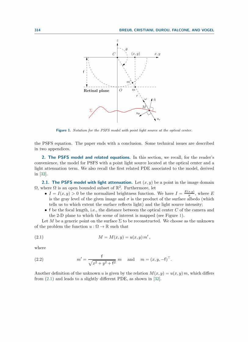
Figure 1. Notation for the PSFS model with point light source at the optical center.

the PSFS equation. The paper ends with a conclusion. Some technical issues are describedin two appendices.

2. The PSFS model and related equations. In this section, we recall, for the reader’sconvenience, the model for PSFS with a point light source located at the optical center and alight attenuation term. We also recall the first related PDE associated to the model, derivedin [32].

2.1. The PSFS model with light attenuation. Let (x, y) be a point in the image domainΩ, where Ω is an open bounded subset of R2. Furthermore, let

• I = I(x, y) > 0 be the normalized brightness function. We have I = E(x,y)σ , where E

is the gray level of the given image and σ is the product of the surface albedo (whichtells us to which extent the surface reflects light) and the light source intensity;

• f be the focal length, i.e., the distance between the optical center C of the camera andthe 2-D plane to which the scene of interest is mapped (see Figure 1).

Let M be a generic point on the surface Σ to be reconstructed. We choose as the unknownof the problem the function u : Ω → R such that

(2.1) M = M(x, y) = u(x, y)m′ ,

where

(2.2) m′ =f√

x2 + y2 + f2m and m = (x, y,−f)�.

Another definition of the unknown u is given by the relation M(x, y) = u(x, y)m, which differsfrom (2.1) and leads to a slightly different PDE, as shown in [32].


Note that, according to this notation, u > 0 holds as the depicted scene is in front ofthe camera. We denote by r(x, y) the distance between the point light source and the pointM(x, y) on the surface. It holds that u(x, y) = r(x, y)/f, since the light source locationcoincides with the optical center.

The model associated to the PSFS problem is obtained by the image irradiance equation,

(2.3) R(n(x, y)) = I(x, y),

making explicit the unit normal n to the surface and the reflectance function R which givesthe value of the light reflection on the surface as a function of its normal.

We denote by ω(x, y) the unit vector representing the light source direction at the pointM(x, y) (note that in the classic SFS model this vector is constant):

(2.4) ω(x, y) =(−x,−y, f)�√x2 + y2 + f2

.

Adding the assumptions of a light attenuation term and of a Lambertian surface, the functionR is defined as

(2.5) R(n(x, y)) =ω(x, y) · n(x, y)

r(x, y)2,

with an attenuation factor which is equal to the inverse of the squared distance from thesource. Expression (2.5) would still hold for any location of the point light source, but thesame would not be true for the equality u(x, y) = r(x, y)/f or for (2.4). The case of a lightsource coinciding with the optical center corresponds more or less to endoscopic images [25]and to photographs taken at short distances with the camera flash [32]. Another considerableadvantage of the PSFS model using a point light source at the optical center is that there isno shadow in the image.

Finally, by (2.3) and (2.5) we obtain the PSFS equation

(2.6)ω(x, y) · n(x, y)

r(x, y)2= I(x, y).

2.2. The corresponding Hamilton–Jacobi equation. In order to write the correspondingPDE, it is useful to introduce the new unknown v = ln(u) (we recall that u > 0). Equation(2.6) can be written as a static Hamilton–Jacobi equation (see [31, 32] and Appendix A fordetails),

(2.7) H(x, y, v,∇v) :=I(x, y)

Q(x, y)f2 W (x, y,∇v)− e−2v(x,y) = 0, (x, y) ∈ Ω,

where

(2.8) Q(x, y) :=f√

x2 + y2 + f2

(which is equal to |cos θ|; cf. Figure 1) and

(2.9) W (x, y,∇v) :=√f2‖∇v‖2 + (∇v · (x, y))2 +Q(x, y)2


(‖ · ‖ denotes the Euclidean norm). Note that W (x, y,∇v) is convex with respect to ∇v ∈ R2,

and then the same property holds for the Hamiltonian H.The existence and uniqueness of the viscosity solution of (2.7) is proved in [32]. In the

same paper some possible choices for the boundary conditions are discussed.Equation (2.7) also admits a “control formulation” which can be helpful. In [32] it is

shown that v is the solution of the following Hamilton–Jacobi–Bellman-like equation:

(2.10) −e−2v(x,y) + supa∈B(0,1)

{−b(x, y, a) · ∇v(x, y)− �(x, y, a)} = 0,

where B(0, 1) denotes the closed unit ball in R2 and the other terms in (2.10) are defined as

follows:

(2.11) �(x, y, a) := −I(x, y) f2√

1− ‖a‖2 , b(x, y, a) := −JGTDGa ,

with

(2.12) J(x, y) :=I(x, y)

Q(x, y)f2 = I(x, y)f

√f2 + x2 + y2 ,

(2.13) G(x, y) :=

⎧⎪⎪⎨⎪⎪⎩1√

x2+y2

(y −xx y

)if (x, y) �= (0, 0),(

1 00 1

)if (x, y) = (0, 0),

(2.14) D(x, y) :=

(f 0

0√

f2 + x2 + y2

).

3. Ambiguities. In this section we show that the model presented above suffers from anambiguity which shares some features with the classic concave/convex ambiguity. We alsoshow in detail in which case it is numerically possible to reconstruct the expected surface andin which case a different surface is computed.

3.1. The ambiguity in the model. In order to prove the existence of two different surfacesassociated to the same brightness function I, it is convenient to reformulate the problem instandard spherical coordinates (r, θ, φ): the parameters of an image point m(θ, φ) are now theangles θ and φ, which are, respectively, the colatitude and the longitude of the conjugatedobject point M(θ, φ), with respect to the camera coordinate system (Cxyz). Let us notethat only the object points M(θ, φ) such that θ ∈ ]π/2, π] are visible (see Figure 1), whereasφ ∈ [0, 2π[. Given a brightness function I(θ, φ), we are looking for a surface Σ in the formr = r(θ, φ) such that

(3.1)ω(θ, φ) · n(θ, φ)

r(θ, φ)2= I(θ, φ).

A generic point M has coordinates

(3.2) M(θ, φ) =

⎛⎝ r(θ, φ) sin θ cosφr(θ, φ) sin θ sinφ

r(θ, φ) cos θ

⎞⎠(Cxyz)


with respect to the coordinate system (Cxyz). We now introduce the local orthonormal basisS = (ur, uθ, uφ) of R

3 defined by

(3.3) ur :=M(θ, φ)

r(θ, φ), uθ :=

∂θur‖∂θur‖ , and uφ :=

∂φur‖∂φur‖ ,

which depends on the point M (see Figure 1). The expression of n in this new basis is (seeAppendix B for details)

(3.4) n(θ, φ) =1

((r2 + rθ2) sin2 θ + rφ2)1/2

⎛⎝ −r sin θrθ sin θrφ

⎞⎠S

,

where the dependence of r, rθ, and rφ on (θ, φ) is omitted. Using (3.4) and considering thatω coincides with −ur (since the point light source is located at the optical center), (3.1) canbe rewritten as

(3.5) r2(r2 + rθ

2 +rφ

2

sin2 θ

)=

1

I2.

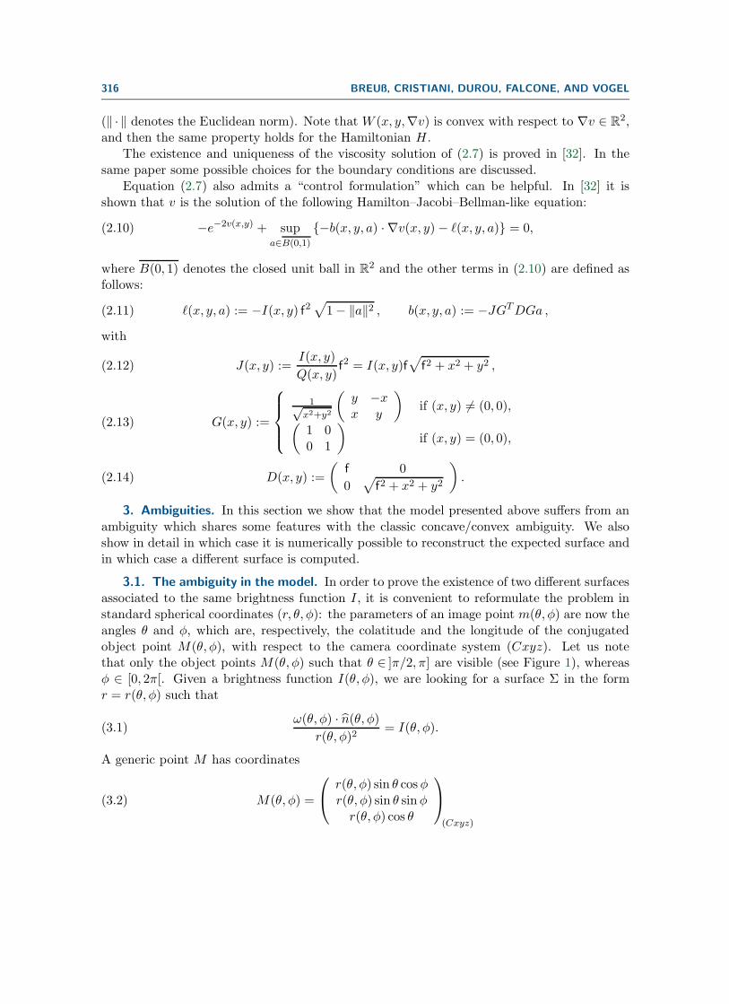
We now return to our purpose. We choose as reference surface Σ the hemisphere r(θ, φ) ≡ 1,where (θ, φ) ∈ ]π/2, π] × [0, 2π[, which is associated to the brightness function IΣ(θ, φ) ≡ 1(see Figure 2).

1

Σ

−1

z

C x

Figure 2. Hemisphere Σ: Do other surfaces give the same brightness function IΣ ≡ 1?

Then, we look for other surfaces which are not isometric to Σ but give the same brightnessfunction. For the sake of simplicity, let us limit our search to the surfaces which are circularlysymmetric around the optical axis Cz, i.e., to the functions r of the form r(θ, φ) = r(θ).Equation (3.5) is thus simplified to the ordinary differential equation

(3.6) r2(r2 + rθ2) =

1

IΣ2 = 1,

which can be rewritten as

(3.7)r dr√1− r4

= ±dθ


since (3.6) imposes r ≤ 1. Integrating (3.7), we obtain the following solutions depending on aparameter θ0, which is a constant of integration:

(3.8) rθ0(θ) =√

cos(2(θ − θ0)).

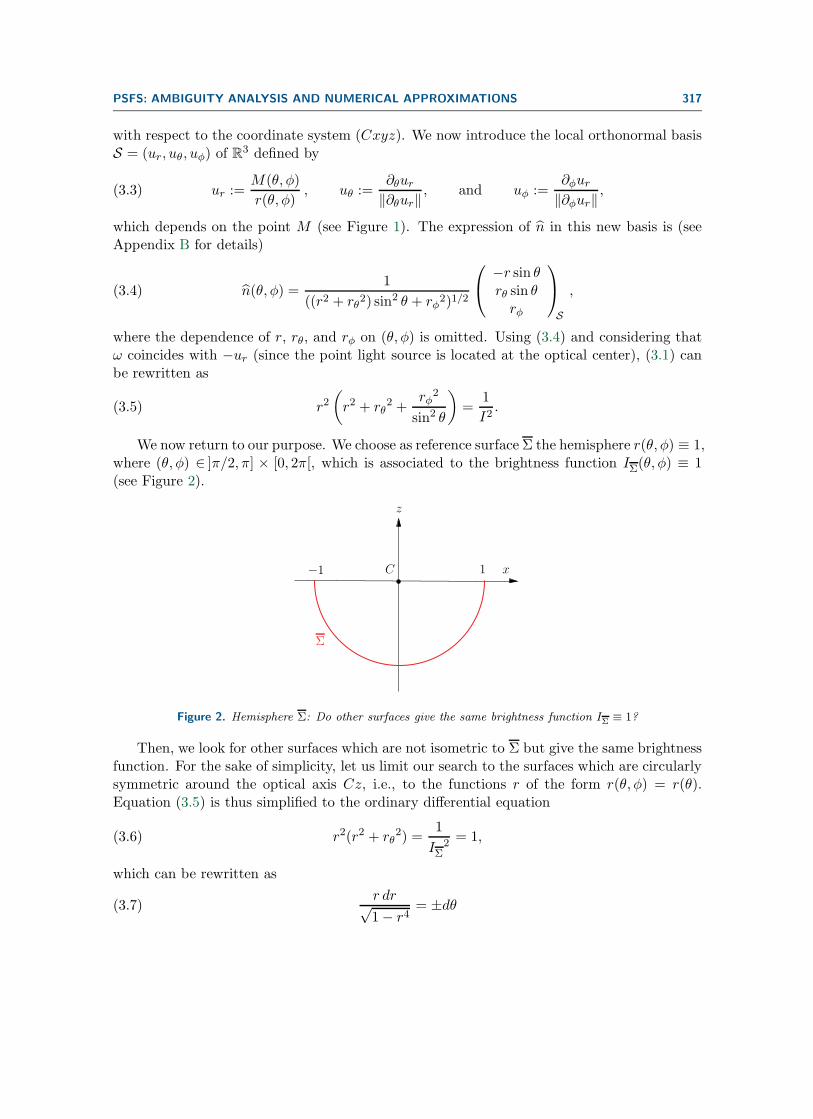
Surfaces Σ. Let us denote as Σθ0 the surface of the equation r = rθ0(θ). Note that (3.8)imposes that θ ∈ ]θ0 − π/4, θ0 + π/4[ (bounds excluded because r > 0). Since θ ∈ ]π/2, π] bydefinition, each surface Σθ0 has the same brightness I ≡ 1 as Σ in a part Dθ0 of the imageplane, i.e., in its domain of definition, which is circularly symmetric around the optical axisCz and contains the points such that θ ∈ Iθ0 = ]θ0−π/4, θ0+π/4[∩ ]π/2, π]. If we require Dθ0

to be nonempty and to contain θ = π, i.e., the origin O in the image plane, this implies thatthe parameter θ0 in (3.8) is in the interval ]3π/4, 5π/4[. Then, we see that Iθ0 = ]θ0 − π/4, π]and that Dθ0 is a disc of center O and of radius ρθ0 = f tan(5π/4 − θ0).

Since all the surfaces Σθ0 , for θ0 ∈ ]3π/4, 5π/4[, are circularly symmetric around the opticalaxis Cz, we can simplify the 3-D setting of spherical coordinates to two dimensions, omittingthe angle describing the location of points with respect to the y-axis. Doing so, we haverepresented the four surfaces Σθ0 which correspond to θ0 = 3π/4+, θ0 = 7π/8, θ0 = π, andθ0 = 9π/8 (cf. Figure 3). Note that among those surfaces, only Σπ is differentiable everywhere(see Figure 3(c)). We thus have found two differentiable surfaces Σ and Σπ which give exactlythe same image in the disc Dπ = (O, f) under the PSFS model with point light source at theoptical center and light attenuation term.

It is important to stress that all other surfaces Σθ0 , for θ0 ∈ ]3π/4, π[∪ ]π, 5π/4[, have aunique singularity at their intersection with the optical axis (see Figures 3(a), 3(b), and 3(d)).

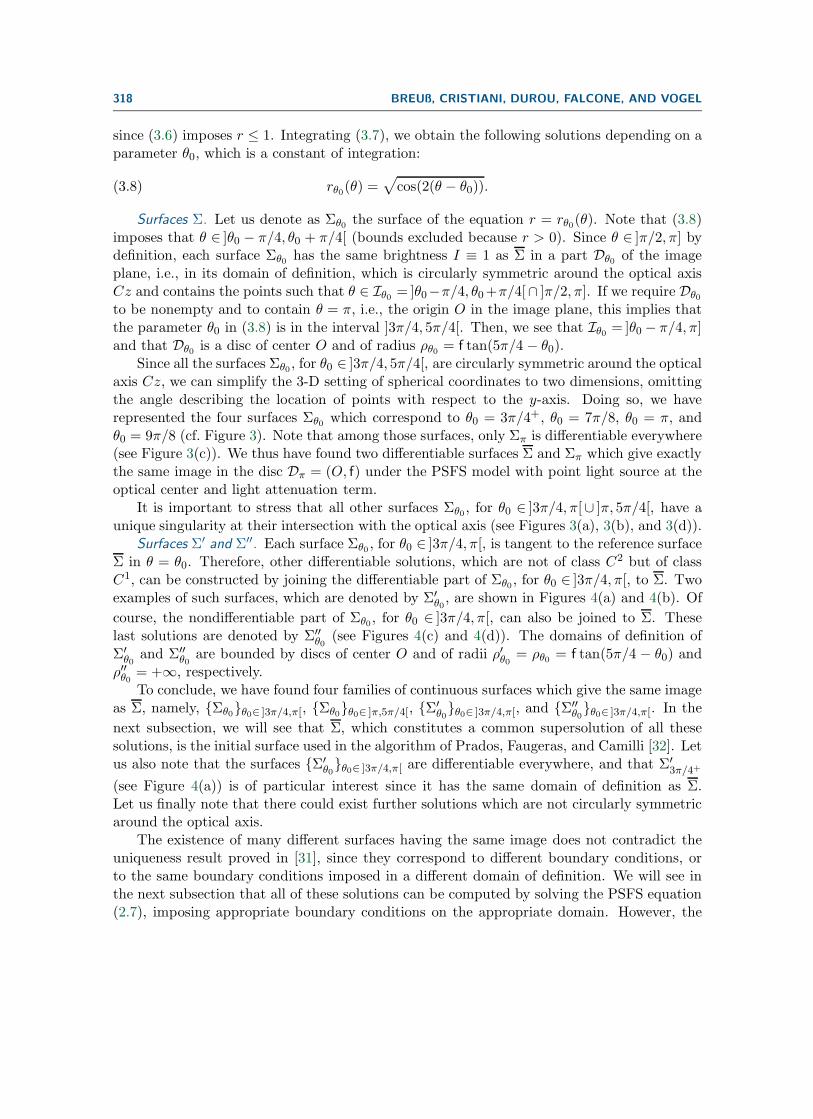
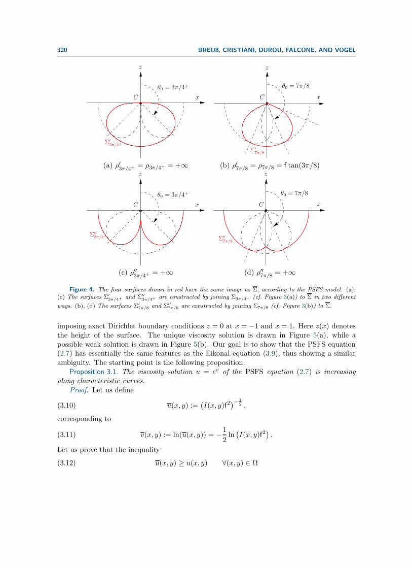
Surfaces Σ′ and Σ′′. Each surface Σθ0 , for θ0 ∈ ]3π/4, π[, is tangent to the reference surfaceΣ in θ = θ0. Therefore, other differentiable solutions, which are not of class C2 but of classC1, can be constructed by joining the differentiable part of Σθ0 , for θ0 ∈ ]3π/4, π[, to Σ. Twoexamples of such surfaces, which are denoted by Σ′

θ0, are shown in Figures 4(a) and 4(b). Of

course, the nondifferentiable part of Σθ0 , for θ0 ∈ ]3π/4, π[, can also be joined to Σ. Theselast solutions are denoted by Σ′′

θ0(see Figures 4(c) and 4(d)). The domains of definition of

Σ′θ0

and Σ′′θ0

are bounded by discs of center O and of radii ρ′θ0 = ρθ0 = f tan(5π/4 − θ0) andρ′′θ0 = +∞, respectively.

To conclude, we have found four families of continuous surfaces which give the same imageas Σ, namely, {Σθ0}θ0∈ ]3π/4,π[, {Σθ0}θ0∈ ]π,5π/4[, {Σ′

θ0}θ0∈ ]3π/4,π[, and {Σ′′

θ0}θ0∈ ]3π/4,π[. In the

next subsection, we will see that Σ, which constitutes a common supersolution of all thesesolutions, is the initial surface used in the algorithm of Prados, Faugeras, and Camilli [32]. Letus also note that the surfaces {Σ′

θ0}θ0∈ ]3π/4,π[ are differentiable everywhere, and that Σ′

3π/4+

(see Figure 4(a)) is of particular interest since it has the same domain of definition as Σ.Let us finally note that there could exist further solutions which are not circularly symmetricaround the optical axis.

The existence of many different surfaces having the same image does not contradict theuniqueness result proved in [31], since they correspond to different boundary conditions, orto the same boundary conditions imposed in a different domain of definition. We will see inthe next subsection that all of these solutions can be computed by solving the PSFS equation(2.7), imposing appropriate boundary conditions on the appropriate domain. However, the


Σ3π/4+

C

z

π/2

θ0 = 3π/4+

x

Σ7π/8

xC

z

θ0 = 7π/8

(a) ρ3π/4+ = +∞ (b) ρ7π/8 = f tan(3π/8)

C

z

x

θ0 = π

Σπ

C x

θ0 = 9π/8

z

Σ9π/8

(c) ρπ = f (d) ρ9π/8 = f tan(π/8)

Figure 3. The four surfaces Σ3π/4+ , Σ7π/8, Σπ, and Σ9π/8 drawn in red, which are circularly symmetric

around the optical axis Cz, have the same image with uniform gray level I ≡ 1 as the hemisphere Σ shown inFigure 2, according to the PSFS model. They belong to the continuous family {Σθ0}θ0∈ ]3π/4,5π/4[.

counterexample exhibited in this subsection suffices to prove that the PSFS model is stillambiguous, even if only the surfaces defined on the whole image plane are considered: apartfrom Σ, Σ′

3π/4+ is differentiable everywhere, whereas all the surfaces Σ′′θ0, for θ0 ∈ ]3π/4, π[,

are other weak solutions of the same problem.

3.2. Viscosity and weak solutions. In this subsection we investigate when the ambiguityarises solving the PSFS equation (2.7). The uniqueness of the viscosity solution of (2.7) wasproved in [32] (see also [30]). Nevertheless, the uniqueness of the viscosity solution does notsolve the problem of the model ambiguity, because we could be interested in the reconstructionof a surface described not by the viscosity solution but rather by another weak solution. Thisis a well-known issue in orthographic SFS with light beam parallel to the optical axis. Let usconsider the simple case of a one-dimensional (1-D) gray level image with constant brightnessfunction I(x) ≡ √

2/2, and let us solve the SFS problem by means of the Eikonal equation

(3.9) |z′(x)| =√

1

I2(x)− 1 , x ∈ [−1, 1],


Σ′3π/4+

C

z

θ0 = 3π/4+

x

z

C x

θ0 = 7π/8

Σ′7π/8

(a) ρ′3π/4+ = ρ3π/4+ = +∞ (b) ρ′7π/8 = ρ7π/8 = f tan(3π/8)

Σ′′3π/4+

C

z

θ0 = 3π/4+

x

Σ′′7π/8

z

C x

θ0 = 7π/8

(c) ρ′′3π/4+ = +∞ (d) ρ′′7π/8 = +∞

Figure 4. The four surfaces drawn in red have the same image as Σ, according to the PSFS model. (a),(c) The surfaces Σ′

3π/4+ and Σ′′3π/4+ are constructed by joining Σ3π/4+ (cf. Figure 3(a)) to Σ in two different

ways. (b), (d) The surfaces Σ′7π/8 and Σ′′

7π/8 are constructed by joining Σ7π/8 (cf. Figure 3(b)) to Σ.

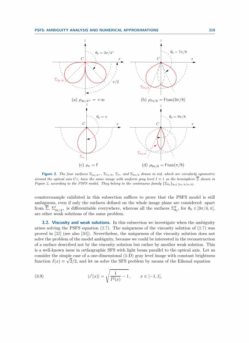
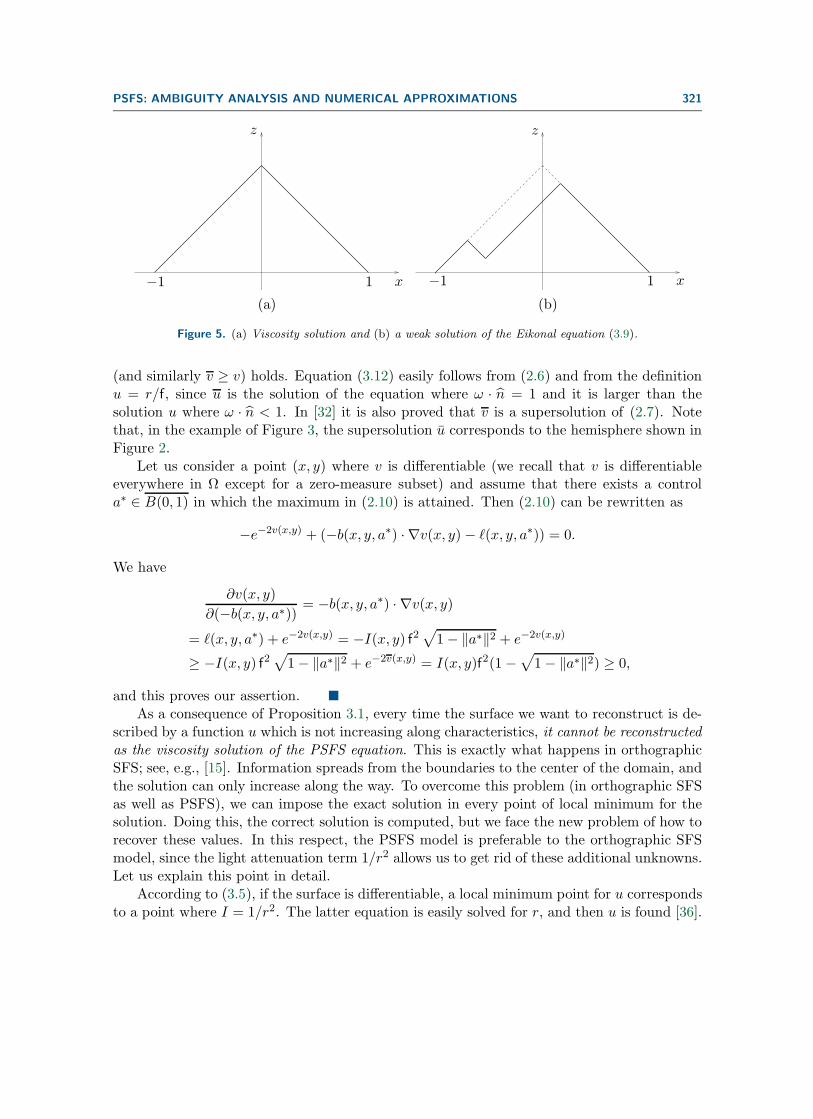
imposing exact Dirichlet boundary conditions z = 0 at x = −1 and x = 1. Here z(x) denotesthe height of the surface. The unique viscosity solution is drawn in Figure 5(a), while apossible weak solution is drawn in Figure 5(b). Our goal is to show that the PSFS equation(2.7) has essentially the same features as the Eikonal equation (3.9), thus showing a similarambiguity. The starting point is the following proposition.

Proposition 3.1. The viscosity solution u = ev of the PSFS equation (2.7) is increasingalong characteristic curves.

Proof. Let us define

(3.10) u(x, y) :=(I(x, y)f2

)− 12 ,

corresponding to

(3.11) v(x, y) := ln(u(x, y)) = −1

2ln

(I(x, y)f2

).

Let us prove that the inequality

(3.12) u(x, y) ≥ u(x, y) ∀(x, y) ∈ Ω


x

z

1−1 x

z

1−1

(a) (b)

Figure 5. (a) Viscosity solution and (b) a weak solution of the Eikonal equation (3.9).

(and similarly v ≥ v) holds. Equation (3.12) easily follows from (2.6) and from the definitionu = r/f, since u is the solution of the equation where ω · n = 1 and it is larger than thesolution u where ω · n < 1. In [32] it is also proved that v is a supersolution of (2.7). Notethat, in the example of Figure 3, the supersolution u corresponds to the hemisphere shown inFigure 2.

Let us consider a point (x, y) where v is differentiable (we recall that v is differentiableeverywhere in Ω except for a zero-measure subset) and assume that there exists a controla∗ ∈ B(0, 1) in which the maximum in (2.10) is attained. Then (2.10) can be rewritten as

−e−2v(x,y) + (−b(x, y, a∗) · ∇v(x, y) − �(x, y, a∗)) = 0.

We have

∂v(x, y)

∂(−b(x, y, a∗))= −b(x, y, a∗) · ∇v(x, y)

= �(x, y, a∗) + e−2v(x,y) = −I(x, y) f2√

1− ‖a∗‖2 + e−2v(x,y)

≥ −I(x, y) f2√1− ‖a∗‖2 + e−2v(x,y) = I(x, y)f2(1−

√1− ‖a∗‖2) ≥ 0,

and this proves our assertion.As a consequence of Proposition 3.1, every time the surface we want to reconstruct is de-

scribed by a function u which is not increasing along characteristics, it cannot be reconstructedas the viscosity solution of the PSFS equation. This is exactly what happens in orthographicSFS; see, e.g., [15]. Information spreads from the boundaries to the center of the domain, andthe solution can only increase along the way. To overcome this problem (in orthographic SFSas well as PSFS), we can impose the exact solution in every point of local minimum for thesolution. Doing this, the correct solution is computed, but we face the new problem of how torecover these values. In this respect, the PSFS model is preferable to the orthographic SFSmodel, since the light attenuation term 1/r2 allows us to get rid of these additional unknowns.Let us explain this point in detail.

According to (3.5), if the surface is differentiable, a local minimum point for u correspondsto a point where I = 1/r2. The latter equation is easily solved for r, and then u is found [36].


This means that the light attenuation term allows us to compute the correct solution exactlywhere we need to impose it. It turns out from (2.6) that these points are also those whereω · n = 1, which characterizes the so-called singular points of the orthographic SFS model [20].Let us stress that the possibility of computing the correct solution at (differentiable) singularpoints is a major feature of the PSFS model which distinguishes it from other models in thefield.

As we will see in section 4, the numerical resolution of the PSFS equation needs to set upan iterative procedure, and then an initial guess for u has to be given in order to start thealgorithm. Let us denote that initial guess by u(0). If we choose u(0) as

(3.13) u(0) := u,

the algorithm starts from a function which is actually the correct solution of (2.6) at all pointswhere ω · n = 1, and is larger than the correct solution elsewhere. Since the informationpropagates from the smallest to the largest values, the values larger than the correct ones donot influence the correct ones. Then the values at the local minimum points remain fixed,becoming characteristic sources, while the other values decrease, converging in the limit tothe viscosity solution. Note that the initial guess (3.13) corresponds to the initial guess for vsuggested in [32], namely

(3.14) v(0) := v.

We conclude that, when the surface is differentiable and local minimum points are notlocated at the boundary, we can actually solve the PSFS problem with no boundary data andno ambiguity, since the right solution at the local minima can be achieved automatically bychoosing a suitable initial guess for the iterative algorithm used to solve the equation.

Otherwise, the method described above cannot always be applied. In particular, themethod fails whenever one of the following conditions holds true: (1) a point of nondifferen-tiability for the surface is a minimum point or (2) local minimum points coincide with theboundaries, and state constraint boundary conditions are used. In these cases, the initial guess(3.13) is not able to impose the right values automatically, and the reconstructed surface willnot be the expected one.

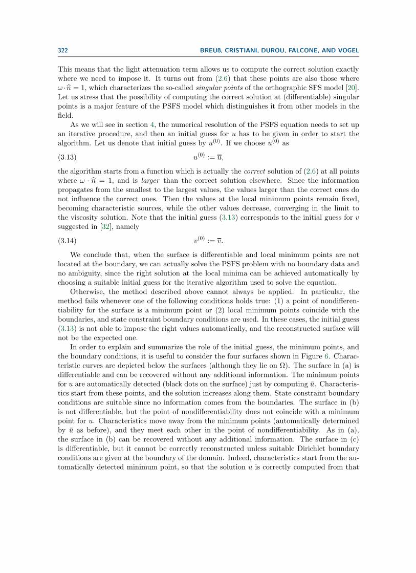
In order to explain and summarize the role of the initial guess, the minimum points, andthe boundary conditions, it is useful to consider the four surfaces shown in Figure 6. Charac-teristic curves are depicted below the surfaces (although they lie on Ω). The surface in (a) isdifferentiable and can be recovered without any additional information. The minimum pointsfor u are automatically detected (black dots on the surface) just by computing u. Characteris-tics start from these points, and the solution increases along them. State constraint boundaryconditions are suitable since no information comes from the boundaries. The surface in (b)is not differentiable, but the point of nondifferentiability does not coincide with a minimumpoint for u. Characteristics move away from the minimum points (automatically determinedby u as before), and they meet each other in the point of nondifferentiability. As in (a),the surface in (b) can be recovered without any additional information. The surface in (c)is differentiable, but it cannot be correctly reconstructed unless suitable Dirichlet boundaryconditions are given at the boundary of the domain. Indeed, characteristics start from the au-tomatically detected minimum point, so that the solution u is correctly computed from that


Σ

C

Σ

C

(a) (b)

Σ

ambiguity

CC

Σ

ambiguity

(c) (d)

Figure 6. Four surfaces with different properties. Characteristic curves are depicted below the surfaces. (a)Differentiable surface, correctly reconstructed imposing state constraint boundary conditions, starting from thetwo singular points automatically detected (black dots). (b) Nondifferentiable surface, correctly reconstructedas before. (c) Differentiable surface with ambiguity if state constraint boundary conditions are imposed. Theambiguity is limited to the region where u should decrease starting from the source points (black dot). (d)Nondifferentiable surface with ambiguity. The nondifferentiable point is not recognized as a source by the initialguess.

point as long as it increases. Imposing state constraint boundary conditions, the viscositysolution to (2.7) near the right-hand boundary corresponds to another surface with the samebrightness function. The surface in (d) is not differentiable, and the point of nondifferentia-bility coincides with a minimum point. As the correct computation of minimum points usingu relies on the differentiability there, this minimum point is not detected, and the viscositysolution to (2.7) does not correspond to this surface on a large part of the domain. Here stateconstraints are suitable, and the surface is correctly reconstructed near the boundaries. Toobtain the correct surface, the value of u at the nondifferentiable point should be given.

At this point it is interesting to compare the classic concave/convex ambiguity in ortho-graphic SFS with the ambiguity shown for PSFS. First, the two ambiguities can both befixed by assigning the exact value of the solution at the sources of characteristics. Second,they are both caused by an ambiguity in the image irradiance equation (2.3). For the PSFS


equation (2.6), for any ω there is more than one couple (n, r) associated to the same I. Thisis similar to what happens in the orthographic SFS, where, for any ω, there is more than onen associated to the same I. On the other hand, the concave/convex ambiguity is related tothe possible degeneration of the Eikonal equation, which is instead not possible in the PSFSequation with light attenuation term. In fact, for the classical SFS, the right-hand side ofthe Eikonal equation (3.9) vanishes at singular points, causing a lack of uniqueness even forregular solutions. This situation does not appear in (2.7), due to the presence of the lightattenuation term.

Following our previous discussion, we end this section by giving a precise definition of theambiguity appearing in the PSFS model.

Definition 3.2. Let Σ and Σ be two piecewise continuous surfaces defined on the samedomain Ω. Let us denote by Γ and Γ their set of discontinuities, respectively. We say that Σand Σ are ambiguous with respect to the PSFS model with attenuation term (A-ambiguousin short) if they are piecewise differentiable on Ω \ Γ and Ω \ Γ, respectively, and they areassociated to the same brightness function I according to the PSFS model.

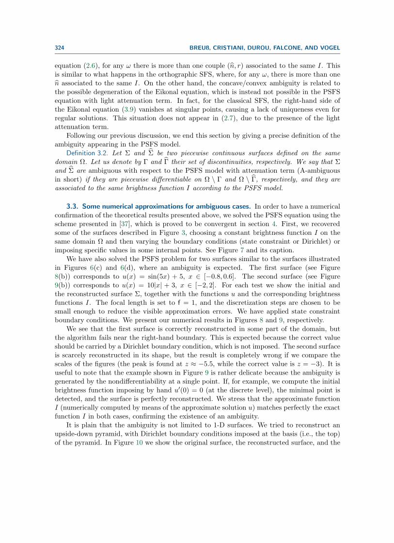
3.3. Some numerical approximations for ambiguous cases. In order to have a numericalconfirmation of the theoretical results presented above, we solved the PSFS equation using thescheme presented in [37], which is proved to be convergent in section 4. First, we recoveredsome of the surfaces described in Figure 3, choosing a constant brightness function I on thesame domain Ω and then varying the boundary conditions (state constraint or Dirichlet) orimposing specific values in some internal points. See Figure 7 and its caption.

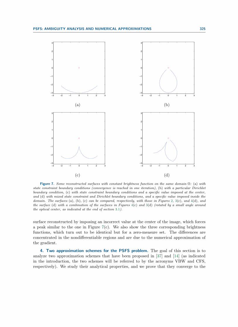
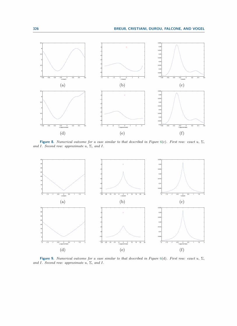
We have also solved the PSFS problem for two surfaces similar to the surfaces illustratedin Figures 6(c) and 6(d), where an ambiguity is expected. The first surface (see Figure8(b)) corresponds to u(x) = sin(5x) + 5, x ∈ [−0.8, 0.6]. The second surface (see Figure9(b)) corresponds to u(x) = 10|x| + 3, x ∈ [−2, 2]. For each test we show the initial andthe reconstructed surface Σ, together with the functions u and the corresponding brightnessfunctions I. The focal length is set to f = 1, and the discretization steps are chosen to besmall enough to reduce the visible approximation errors. We have applied state constraintboundary conditions. We present our numerical results in Figures 8 and 9, respectively.

We see that the first surface is correctly reconstructed in some part of the domain, butthe algorithm fails near the right-hand boundary. This is expected because the correct valueshould be carried by a Dirichlet boundary condition, which is not imposed. The second surfaceis scarcely reconstructed in its shape, but the result is completely wrong if we compare thescales of the figures (the peak is found at z ≈ −5.5, while the correct value is z = −3). It isuseful to note that the example shown in Figure 9 is rather delicate because the ambiguity isgenerated by the nondifferentiability at a single point. If, for example, we compute the initialbrightness function imposing by hand u′(0) = 0 (at the discrete level), the minimal point isdetected, and the surface is perfectly reconstructed. We stress that the approximate functionI (numerically computed by means of the approximate solution u) matches perfectly the exactfunction I in both cases, confirming the existence of an ambiguity.

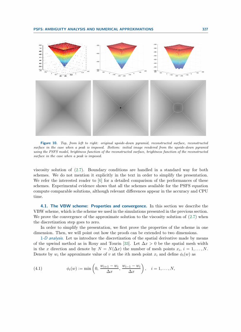
It is plain that the ambiguity is not limited to 1-D surfaces. We tried to reconstruct anupside-down pyramid, with Dirichlet boundary conditions imposed at the basis (i.e., the top)of the pyramid. In Figure 10 we show the original surface, the reconstructed surface, and the


−3 −2 −1 0 1 2 3−3

−2

−1

0

1

2

3

−3 −2 −1 0 1 2 3−3

−2

−1

0

1

2

3

(a) (b)

−3 −2 −1 0 1 2 3−3

−2

−1

0

1

2

3

−3 −2 −1 0 1 2 3−3

−2

−1

0

1

2

3

(c) (d)

Figure 7. Some reconstructed surfaces with constant brightness function on the same domain Ω: (a) withstate constraint boundary conditions (convergence is reached in one iteration), (b) with a particular Dirichletboundary condition, (c) with state constraint boundary conditions and a specific value imposed at the center,and (d) with mixed state constraint and Dirichlet boundary conditions, and a specific value imposed inside thedomain. The surfaces (a), (b), (c) can be compared, respectively, with those in Figures 2, 3(c), and 4(d), andthe surface (d) with a combination of the surfaces in Figures 4(c) and 3(d) (rotated by a small angle aroundthe optical center, as indicated at the end of section 3.1).

surface reconstructed by imposing an incorrect value at the center of the image, which forcesa peak similar to the one in Figure 7(c). We also show the three corresponding brightnessfunctions, which turn out to be identical but for a zero-measure set. The differences areconcentrated in the nondifferentiable regions and are due to the numerical approximation ofthe gradient.

4. Two approximation schemes for the PSFS problem. The goal of this section is toanalyze two approximation schemes that have been proposed in [37] and [14] (as indicatedin the introduction, the two schemes will be referred to by the acronyms VBW and CFS,respectively). We study their analytical properties, and we prove that they converge to the


−0.8 −0.6 −0.4 −0.2 0 0.2 0.4 0.63.5

4

4.5

5

5.5

6

6.5

u (exact)−4 −3 −2 −1 0 1 2 3

−7

−6

−5

−4

−3

−2

−1

0

1

Σ (exact)−0.8 −0.6 −0.4 −0.2 0 0.2 0.4 0.6

0.02

0.025

0.03

0.035

0.04

0.045

0.05

0.055

0.06

0.065

I (exact)

(a) (b) (c)

−0.8 −0.6 −0.4 −0.2 0 0.2 0.4 0.63.5

4

4.5

5

5.5

6

6.5

u (approximate)−4 −3 −2 −1 0 1 2 3

−7

−6

−5

−4

−3

−2

−1

0

1

Σ (approximate)−0.8 −0.6 −0.4 −0.2 0 0.2 0.4 0.6

0.02

0.025

0.03

0.035

0.04

0.045

0.05

0.055

0.06

0.065

I (approximate)

(d) (e) (f)

Figure 8. Numerical outcome for a case similar to that described in Figure 6(c). First row: exact u, Σ,and I. Second row: approximate u, Σ, and I.

−2 −1.5 −1 −0.5 0 0.5 1 1.5 20

5

10

15

20

25

30

35

40

u (exact)−25 −20 −15 −10 −5 0 5 10 15 20 25

−12

−10

−8

−6

−4

−2

0

2

Σ (exact)−2 −1.5 −1 −0.5 0 0.5 1 1.5 20

0.005

0.01

0.015

0.02

0.025

0.03

0.035

I (exact)

(a) (b) (c)

−2 −1.5 −1 −0.5 0 0.5 1 1.5 20

5

10

15

20

25

30

35

40

u (approximate)−25 −20 −15 −10 −5 0 5 10 15 20 25

−12

−10

−8

−6

−4

−2

0

2

Σ (approximate)−2 −1.5 −1 −0.5 0 0.5 1 1.5 20

0.005

0.01

0.015

0.02

0.025

0.03

0.035

I (approximate)

(d) (e) (f)

Figure 9. Numerical outcome for a case similar to that described in Figure 6(d). First row: exact u, Σ,and I. Second row: approximate u, Σ, and I.


−200−100

0100

200

−200−100

0100

200−500

−450

−400

−350

−200−100

0100

200

−200−100

0100

200−480

−460

−440

−420

−400

−380

−360

−340

Figure 10. Top, from left to right: original upside-down pyramid, reconstructed surface, reconstructedsurface in the case when a peak is imposed. Bottom: initial image rendered from the upside-down pyramidusing the PSFS model, brightness function of the reconstructed surface, brightness function of the reconstructedsurface in the case when a peak is imposed.

viscosity solution of (2.7). Boundary conditions are handled in a standard way for bothschemes. We do not mention it explicitly in the text in order to simplify the presentation.We refer the interested reader to [6] for a detailed comparison of the performances of theseschemes. Experimental evidence shows that all the schemes available for the PSFS equationcompute comparable solutions, although relevant differences appear in the accuracy and CPUtime.

4.1. The VBW scheme: Properties and convergence. In this section we describe theVBW scheme, which is the scheme we used in the simulations presented in the previous section.We prove the convergence of the approximate solution to the viscosity solution of (2.7) whenthe discretization step goes to zero.

In order to simplify the presentation, we first prove the properties of the scheme in onedimension. Then, we will point out how the proofs can be extended to two dimensions.

1-D analysis. Let us introduce the discretization of the spatial derivative made by meansof the upwind method as in Rouy and Tourin [33]. Let Δx > 0 be the spatial mesh widthin the x direction and denote by N = N(Δx) the number of mesh points xi, i = 1, . . . , N .Denote by wi the approximate value of v at the ith mesh point xi and define φi(w) as

(4.1) φi(w) := min

(0,

wi+1 −wi

Δx,wi−1 − wi

Δx

), i = 1, . . . , N,


where w = (w1, . . . , wN ). The approximate gradient is given by

(4.2) ∇v(xi) ≈ ∇wi :=

{ −φi(w) if φi(w) =wi−1−wi

Δx ,φi(w) otherwise.

By the above upwind discretization, one gets the discrete operator

(4.3) Li(w) :=

(−Iif

2

Qi

√(f∇wi)2 + (xi∇wi)2 +Q2

i + e−2wi

)and can write the discrete version of (2.7) as

(4.4) Li(w) = 0, i = 1, . . . , N.

Let us introduce the parameter τ > 0 and the function Gτ : RN → RN defined componentwise

as follows:

(4.5) Gτi (w) := wi + τLi(w) , i = 1, . . . , N.

Equation (4.4) can be written in fixed point form as

(4.6) w = Gτ (w).

Note that Gτi ∈ C0(RN ) and is piecewise differentiable in R

N . We describe important struc-tural properties of Gτ in the following proposition.

Proposition 4.1. Let Gτ : RN → RN be defined as in (4.5) and let w ′, w ′′ ∈ R

N . Then,there exists τ∗ = τ∗(Δx) > 0 such that

(i) w ′ ≤ w ′′ implies Gτ (w ′) ≤ Gτ (w ′′) for any τ < τ∗ (≤ is intended componentwise);(ii) ‖Gτ (w ′)−Gτ (w ′′)‖∞ < ‖w ′ − w ′′‖∞ for any τ < τ∗.Proof. Let us first assume that the evaluation of (4.2) gives ∇wi =

wi−wi−1

Δx , which implieswi − wi−1 > 0. Then, we have

(4.7)∂Gτ

i (w)

∂wi= 1− τIif

2

Qi

(x2i + f2)wi−wi−1

Δx2√(f2 + x2i )

(wi−wi−1

Δx

)2+Q2

i

− 2τe−2wi ,

(4.8)∂Gτ

i (w)

∂wi−1=

τIif2

Qi

(x2i + f2)wi−wi−1

Δx2√(f2 + x2i )

(wi−wi−1

Δx

)2+Q2

i

,

and

(4.9)∂Gτ

i (w)

∂wi+1= 0.

The term ∂Gτi (w)/∂wi−1 is always positive, whereas ∂Gτ

i (w)/∂wi is positive only for τ suffi-ciently small. Note that the maximal value τ∗ can be explicitly computed by means of (4.7),and the condition τ < τ∗ can be explicitly verified while the algorithm is running.


If ∇wi =wi+1−wi

Δx , we get a similar result. Let us assume now that ∇wi = 0. We get

Gτi (w) = wi − τIif

2 + τe−2wi

and then∂Gτ

i (w)

∂wi= 1− 2τe−2wi ,

∂Gτi (w)

∂wi−1=

∂Gτi (w)

∂wi+1= 0.

Again, the three terms are positive, provided that τ is sufficiently small. This proves (i).Let us denote by JGτ the Jacobian matrix of Gτ . Whatever the evaluation of ∇w gives,

assuming that τ is sufficiently small, we get

(4.10) ‖JGτ ‖∞ = maxi

{∂Gτ

i

∂wi−1+

∂Gτi

∂wi+

∂Gτi

∂wi+1

}= max

i

{1− 2τe−2wi

},

which is always strictly lower than 1, and this ends the proof.The algorithm is implemented in the following iterative form:

(4.11) w(n+1)i = Gτ

i (w(n)) , i = 1, . . . , N, n = 0, 1, . . . .

The initial guess w(0) is given by the discretization of (3.14).Proposition 4.2. Let w(0) be chosen as in (3.14) and let τ∗ be the “constant” defined by

Proposition 4.1. Then, there exists τ∗∗ = τ∗∗(Δx) > 0 such that(i) the algorithm (4.11) converges to the unique fixed point wΔx for any τ < τ∗∗;(ii) if τ < min{τ∗, τ∗∗}, the algorithm converges monotonically decreasing; i.e., for any

i = 1, . . . , N , we have w(n+1)i ≤ w

(n)i , n = 0, 1, . . . .

Proof. In order to apply the Banach fixed point theorem, we have only to show thatGτ : X → X, where X is a compact subset of RN . We choose X = [wmin, wmax]

N , wherewmin and wmax are two constants such that wmin < −1

2 ln(Iif2) and wmax > −1

2 ln(Iif2) for

any i = 1, . . . , N . This ensures that

(4.12) −Iif2 + e−2wmin > 0 for any i

and

(4.13) −Iif2 + e−2wmax < 0 for any i.

Let us fix w ∈ X and i ∈ {1, . . . , N}. The proof is divided into two steps.(a) We prove that Gτ

i (w) ≥ wmin. We have wi = wmin + δ for some 0 ≤ δ ≤ δmax withδmax := wmax − wmin. Since all the components of w are larger than wmin, using (4.2) we get(∇wi)

2 ≤ ( δΔx)

2. Then we have

Gτi (w) = wi + τLi(w) ≥ wmin + δ + τΨ1(δ),

where

Ψ1(δ) :=

⎛⎝−Iif2

Qi

√(fδ

Δx

)2

+

(xi

δ

Δx

)2

+Q2i + e−2(wmin+δ)

⎞⎠ .


Given (4.12), we know that Ψ1(0) = −Iif2+e−2wmin > 0. The function Ψ1(δ) is monotonically

decreasing, and limδ→+∞Ψ1(δ) = −∞. As a consequence, there exists a unique δ0 > 0 suchthat Ψ1(δ0) = 0. If 0 ≤ δ ≤ δ0, we have Ψ1(δ) ≥ 0 and Gτ

i (w) ≥ wmin for any τ . Otherwise,if δ0 < δ ≤ δmax, we choose

τ ≤ δ0−Ψ1(δmax)

,

which guarantees τ ≤ δ−Ψ1(δ)

, and we easily conclude.

(b) Let us now prove that Gτi (w) ≤ wmax. Similarly as before, we have wi = wmax − δ for

some 0 ≤ δ ≤ δmax with δmax := wmax − wmin. Then we have

Gτi (w) = wi + τLi(w) ≤ wmax − δ + τΨ2(δ),

where

Ψ2(δ) :=

(−Iif

2

Qi

√0 + 0 +Q2

i + e−2(wmax−δ)

)=

(−Iif

2 + e−2(wmax−δ)).

Given (4.13), we know that Ψ2(0) = −Iif2+e−2wmax < 0. The function Ψ2(δ) is monotonically

increasing, and limδ→+∞Ψ2(δ) = +∞. As a consequence, there exists a unique δ0 > 0 suchthat Ψ2(δ0) = 0. If 0 ≤ δ ≤ δ0, we have Ψ2(δ) ≤ 0 and Gτ

i (w) ≤ wmax for any τ . Otherwise,if δ0 < δ ≤ δmax, we choose

τ ≤ δ0Ψ2(δmax)

,

which guarantees τ ≤ δΨ2(δ)

, and we easily conclude. This proves Proposition 4.2(i).The choice of the initial guess is the key property in obtaining monotone decreasing con-

vergence to the fixed point. In fact, w(0) is larger than (or equal to) the solution (see section3.2), and Gτ verifies Proposition 4.1(i). This proves Proposition 4.2(ii).

We want to prove convergence of the numerical solution wΔx to the viscosity solution vof (2.7) for Δx → 0. We can rely on the classic results of Barles and Souganidis [2], followingthe same strategy of Rouy and Tourin [33].

Proposition 4.3. Let w(0) be chosen as in (3.14) and let τ∗, τ∗∗ be the “constants” definedby Propositions 4.1 and 4.2. If τ < min{τ∗, τ∗∗}, then the algorithm (4.11) converges to wΔx

for n → +∞, and wΔx converges locally uniformly to v for Δx → 0.Proof. Convergence to wΔx for n → +∞ is proved in Proposition 4.2(i). To prove the

convergence to v, we start proving that the scheme is monotone in the sense given in [2]. Weknow that the fixed point wΔx satisfies the equation

L(w) = 0,

so we will use this form, since in [2] the discrete operator is written in the implicit formS(Δx, x,w(x), w) = 0, where S : R+ ×Ω×R×B(Ω) → R and B(Ω) is the space of boundedfunctions defined on Ω. If the evaluation of (4.2) gives ∇wi =

wi−wi−1

Δx , we have only to prove

that ∂Li(w)∂wi−1

does not change sign. By (4.8) we easily get ∂Li(w)∂wi−1

> 0. If the evaluation of (4.2)

gives ∇wi = wi+1−wi

Δx , we obtain analogously ∂Li(w)∂wi+1

> 0. Finally, if ∇wi = 0, Li does notdepend on wi−1 or wi+1.


The stability and consistency of the scheme are easy to prove. Since the comparisonprinciple for the problem is proved in [32], we know that (2.7) has a unique viscosity solutionv, and we can conclude, by the general convergence result in [2], that the approximate solutionconverges locally uniformly to v.

It is interesting to note that the property pointed out in Proposition 3.1 is preserved in thenumerical approximation. Let us assume that the assumptions of Proposition 4.3 are satisfied.We want to show that

(4.14)

⎧⎪⎪⎨⎪⎪⎩w

(n+1)i > w

(n)i−1 if ∇wi =

wi−wi−1

Δx ,

w(n+1)i > w

(n)i+1 if ∇wi =

wi+1−wi

Δx ,

w(n+1)i = w

(n)i if ∇wi = 0.

If (4.14) holds true, the solution is constructed from the smallest to the largest values, and thenthe solution cannot become lower than the information sources (Dirichlet boundary conditionsor minimum points automatically detected). Let us prove the first line in (4.14). To this end,we first recall that

w(n+1)i = Gτ

i (w(n)) = w

(n)i + τLi(w

(n)).

Note that Proposition 4.2(ii) implies Li(w(n)) < 0 for any i and n. In order to have w

(n+1)i >

w(n)i−1, the parameter τ must be chosen in such a way that

τ |L(w(n))| < w(n)i − w

(n)i−1,

which corresponds to

(4.15) τ <w

(n)i −w

(n)i−1

−Li(w(n)).

Note that the right-hand term in (4.15) is strictly positive. For any fixed Δx, the termLi(w

(n)) → 0 when n → +∞ (this follows by the fact that the algorithm converges to thefixed point). Then, condition (4.15) is always satisfied in the limit.

We can also reobtain the result already proved for the continuous equation. Let us write

w(n+1)i − w

(n)i−1

Δx=

w(n+1)i − w

(n)i

Δx+

w(n)i − w

(n)i−1

Δx.

Since, as we have just seen, w(n+1)i −w

(n)i−1 ≥ 0, and we know that w

(n+1)i −w

(n)i ≤ 0 (because

the algorithm computes a decreasing sequence), we obtain that w(n)i − w

(n)i−1 ≥ 0 for any Δx,

and then, passing to the limit (in the case it exists),

limΔx→0+

w(xi)− w(xi −Δx)

Δx≥ 0,

which corresponds to the fact that the solution is increasing along the characteristic direction.


2-D analysis. The strategy developed in the 1-D case can be easily generalized, and allthe main results still hold. The only difference is a new condition on the experimental set-upwhich is necessary to prove that w1 ≤ w2 implies Gτ (w1) ≤ Gτ (w2).

Assuming a square uniform N ×N grid with Δx = Δy, the scheme is now defined com-ponentwise by

(4.16) Gτi,j(w) := wi,j + τLi,j(w), i, j = 1, . . . , N,

where

Li,j(w) :=(4.17)

− Ii,jQi,j

f2√f2((∇xwi,j)2 + (∇ywi,j)2

)+

(xi∇xwi,j + yj∇ywi,j

)2+Q2

i,j + e−2wi,j .

Let us assume that ∇wi,j is equal to 1Δx (wi,j − wi−1,j , wi,j −wi,j−1). We have

(4.18)∂Gτ

i,j(w)

∂wi−1,j=

τIi,jf2

Qi,j

Aij(w)√Bij(w)

,

where

(4.19) Aij(w) := (x2i + f2)wi,j − wi−1,j

Δx2+ xiyj

wi,j − wi,j−1

Δx2,

Bij(w) := f2(wi,j − wi−1,j

Δx

)2

+ f2(wi,j − wi,j−1

Δx

)2

+

(xiwi,j − wi−1,j

Δx+ yj

wi,j − wi,j−1

Δx

)2

+Q2i,j,(4.20)

and an analogous result for ∂Gτi,j(w)/∂wi,j−1. With no further assumptions, the quantity in

(4.18) can be negative, due to the term xiyj in (4.19), which has no fixed sign. Then, in orderto get the same result as in the 1-D case, namely ‖JGτ ‖∞ = maxi,j

{1− 2τe−2wi,j

}, we need

to assume that

(4.21) (x2i + f2) (wi,j − wi−1,j) + xiyj (wi,j − wi,j−1) ≥ 0

and, analogously, that

(4.22) (y2j + f2) (wi,j − wi,j−1) + xiyj (wi,j − wi−1,j) ≥ 0.

As the conditions (4.21)–(4.22) incorporate a coupling of image dimension and focal length,they imply a condition on the experimental set-up. They are fulfilled if f is sufficiently large,or if the surface is fully contained in the “positive” region {x > 0, y > 0}.


4.2. The CFS scheme: Properties and convergence. In order to simplify the notation,let us prove the result in the 1-D case. Generalization to a higher dimension is trivial, andall the results are preserved. The semidiscrete formulation of the CFS scheme was derived in[13, 14]; we report it here for the reader’s convenience. For any function w : R → R, we definethe semidiscrete operator F h as

(4.23) F h[w](x) := mina∈B(0,1)

{w(x+ hb(x, a)) + h�(x, a)} + he−2w(x).

The iterative algorithm can be written in compact form as

(4.24)

{w(n+1)(x) = F h[w(n)](x) , n = 0, 1, . . . ,

w(0)(x) = −12 ln(I(x)f

2).

As usual, the parameter h must be intended as a fictitious-time discretization step used tointegrate along characteristics in the semi-Lagrangian formulation [18]. We do not considerhere the fully discrete problem in which the operator F h is projected on a grid.

In the following we prove that the sequence generated by the algorithm (4.24) actuallyconverges to some function wh. Note that we employ here an approach that is different fromthe one used in the previous subsection for the analysis of the VBW method. More precisely,we will not prove that the operator F h is a contraction mapping, but we prove that thesequence {w(n)}n≥0 is monotone decreasing and bounded from below.

Proposition 4.4 (boundedness from below). Let w ∈ C0(Ω). For any x ∈ Ω there exist astep h = h(x) > 0 and a constant wmin ∈ R such that

(4.25) w(x) ≥ wmin implies F h[w](x) ≥ wmin.

Proof. Let us consider two cases separately.(i) Let w(x) = wmin. We first note, by the definition of � in (2.11), that �(x, 0) =

mina{�(x, a)}. Second, by the definition of b in (2.11), we have w(x + hb(x, 0)) = w(x) =mina{w(x + hb(x, a))} since the minimum of w is attained at x by assumption. As a conse-quence, the minimum in (4.23) is attained for a∗ = 0. Then,

F h[w](x) = w(x)− hI(x)f2 + he−2w(x) = wmin + h(e−2wmin − I(x)f2

).

Similarly to the VBW case, we choose wmin in such a way that

e−2wmin − I(x)f2 ≥ 0,

and then F h[w](x) ≥ wmin. Note that it is possible to choose such a wmin uniformly in x. Tothis end, it is sufficient to choose wmin ≤ minx∈Ωw(0)(x).

(ii) Let w(x) > wmin. The continuity of w guarantees that there exists a ball B(x, ξ)centered in x of radius ξ such that w(x′) > wmin for every x′ ∈ B(x, ξ). Let us denote by a∗

the argmin appearing in the definition of F h[w]. Defining Δw = w(x+ hb(x, a∗))−wmin, wehave

F h[w](x) = w(x+ hb(x, a∗)) + h�(x, a∗) + he−2w(x)

= wmin +Δw + h(e−2w(x) + �(x, a∗))≥ wmin +Δw + h(0− I(x)f2).


Choosing h in such a way that hmaxa b(x, a) < ξ, we have Δw > 0. Moreover, we notethat Δw does not tend to zero if h tends to zero. The conclusion follows by choosing h ≤Δw/I(x)f2.

Proposition 4.5 (monotonicity). Let us assume that w(n) ∈ C1(Ω) for any n ∈ N. Then, forany n ∈ N there exists a step h = h(n) > 0 such that the sequence defined in (4.24) verifies

w(n+1)(x) ≤ w(n)(x) for any x ∈ Ω.

Proof. We first consider points x such that the corresponding a∗ is equal to zero at thefirst iteration n = 0. These are the points where the initial guess w(0) is actually the correctsolution; see section 3.2. In this case we have

w(1)(x) = w(0)(x)− hI(x)f2 + he−2w(0)(x) = w(0)(x).

Since the solution already reached convergence at these points, we can simply stop the com-putation (so that w(n+1)(x) = w(n)(x) for any n).

Let us now consider a point x such that a∗(x) �= 0 for n = 0. We prove the assertion byinduction on n. We have

w(1)(x) = w(0)(x+ hb(x, a∗)) + h�(x, a∗) + he−2w(0)(x).

Since a∗ �= 0, we have

(4.26) w(0)(x+ hb(x, a∗)) + h�(x, a∗) < w(0)(x+ hb(x, 0)) + h�(x, 0) = w(0)(x)− hI(x)f2,

and then w(1)(x) < w(0)(x) − hI(x)f2 + he−2w(0)(x) = w(0)(x). Note that we could find twodifferent optimal controls a∗1 = 0 and a∗2 �= 0 in which the minimum is attained, so that thestrict inequality in (4.26) does not hold true. This issue can be fixed assuming that in suchan ambiguous case we keep a∗1 as optimal control.

Now we prove that

w(n)(x) < w(n−1)(x) implies w(n+1)(x) < w(n)(x).

We have to prove that F h[w(n)](x) < F h[w(n−1)](x). Let us denote by a∗ the argmin forF h[w(n−1)](x). Note that a∗ is in general different from the argmin for F h[w(n)](x). Then, itis sufficient to show that

w(n)(x+ hb(x, a∗)) + h�(x, a∗) + he−2w(n)(x)

< w(n−1)(x+ hb(x, a∗)) + h�(x, a∗) + he−2w(n−1)(x)

or, analogously, that

w(n)(x+ hb(x, a∗))−w(n−1)(x+ hb(x, a∗)) + h(e−2w(n)(x) − e−2w(n−1)(x)

)< 0.

Since the function z �→ e−2z is differentiable and w(n)(x) ≥ wmin for any n (see Proposition4.4), by Taylor’s expansion we get(

e−2w(n)(x) − e−2w(n−1)(x))< 2e−2wmin

(w(n−1)(x)− w(n)(x)

).


Then, we need only prove that

w(n)(x+ hb(x, a∗))− w(n−1)(x+ hb(x, a∗)) + 2he−2wmin

(w(n−1)(x)− w(n)(x)

)< 0.

Let us define C := 2e−2wmin and again use Taylor’s expansion for w(n) and w(n−1). We have

(1− Ch)w(n)(x) + (Ch− 1)w(n−1)(x)(4.27)

+ hb(x, a∗) ·(∇w(n)(x)−∇w(n−1)(x)

)+O(h2) < 0.

When h tends to zero, the left-hand side of the previous inequality tends to w(n)(x)−w(n−1)(x),which is strictly negative by assumption. Then there exists an h sufficiently small such that(4.27) holds true.

To conclude, let us observe that, assuming I ∈ C1(Ω), we have w(0) ∈ C1(Ω) and thenw(n) ∈ C1(Ω) for any n, since the regularity is preserved by the operator F h. Under thisassumption, the two previous propositions can be applied, and we get the convergence of thesequence defined in (4.24).

Finally, note that the dependence of the step h on x and n is not an issue in the imple-mentation of the numerical approximation because the space is discretized in a finite numberof nodes and the algorithm is stopped after a finite number of iterations.

5. Dealing with discontinuous surfaces. In this section we suggest a simple algorithm todeal with the reconstruction of discontinuous surfaces. Discontinuous surfaces can arise bothbecause of different objects in a scene and because of parts of the object being occluded byother parts of the object due to the projection. Numerical tests performed in [6, 13, 14] clearlyshow that the PSFS algorithm is not able to catch discontinuities of the surface. In fact, ittries to reconstruct a continuous surface with the same brightness function as the originalone. In order to deal with discontinuities, the idea is to first perform a segmentation of theinput image, dividing the domain into several subdomains. The boundaries of the subdomainscorrespond to the curves of discontinuity of the brightness function. Then, we apply the PSFSalgorithm piecewise in every subdomain where the brightness function is continuous. For eachsubdomain, initial data for the iterative schemes are chosen as in (3.14).

It is worth noting that a similar segmentation procedure will not be valid for the ortho-graphic SFS problem. Indeed, splitting the original image into subdomains will result in aneven more complicated problem where several new boundaries have to be taken into account.Since in the orthographic SFS model the gray values do not contain depth information, if noadditional information is available, the segmented SFS problem will be undetermined.

The question arises of which boundary conditions have to be imposed at the boundary ofeach subdomain for the PSFS model. In the following we have always imposed state constraintboundary conditions there. This is a natural choice, since they simply inhibit the propagationof information from outside the segment into the segment. This makes sense, since anyinformation from outside the segment, i.e., across the discontinuity, is unreliable. To imposestate constraint boundary conditions on each segment we simply set on the boundary of thesegment a value larger than the maximal value of the solution inside the segment. An easychoice is to set it equal to the maximum machine number.


(a) (b)

(c) (d)

Figure 11. (a) Input image, (b) input surface, (c) reconstructed surface by a direct application of the PSFSscheme (state constraint boundary conditions), (d) reconstructed surface after segmentation (state constraintboundary conditions).

However, we note that, coherently with the previous results about ambiguity in the PSFSmodel, we cannot guarantee that inside each subdomain the reconstructed surface is theexpected one.

Synthetic input data. We test the new algorithm on a synthetic photograph of an upside-down pyramid over a flat surface. See Figures 11(a) and 11(b) for the input photograph andthe true surface (note that the pyramid hides most of the background).

Applying the PSFS algorithm directly, we obtain the surface depicted in Figure 11(c),where the discontinuity is totally lost. Note that the reconstructed surface has the samebrightness function as the original one. Applying the PSFS algorithm after the segmentation,we have to solve two separate problems (for the pyramid and for the frame). The result isshown in Figure 11(d). This time the background is reconstructed at the right distance; i.e.,the discontinuity is preserved. Nevertheless, the sides of the pyramid and the frame are not


Table 1Errors for the test described in Figure 11.

Algorithm L1 error L∞ error

Direct 8.74% 26.71%

Presegmented 2.55% 4.80%

(a) (b)

-60-50

-40-30

-20-10

-40-30

-20-10

0 10

20 30

40 50

390

400

410

420

430

440

395 400 405 410 415 420 425 430 435 440

-30-20

-10 0

10 20

30 40

-20-10

0 10

20 30

40 50

60

385

390

395

400

405

388 390 392 394 396 398 400 402 404 406

(c) (d)

Figure 12. (a) Real-world input image and (b) its 3-D reconstruction. (c) Separate visualization of themug segment reconstruction and (d) separate visualization of the cup segment reconstruction.

completely flat as they should be. This is due to the fact that state constraint boundaryconditions are not suitable here, because the local minimum points are on the boundary ofthe domain, as in Figure 6(c). For the experiment, we used a 256×256 grid and f = 250. Thereconstruction errors (depth error compared to the ground truth) are summarized in Table 1.

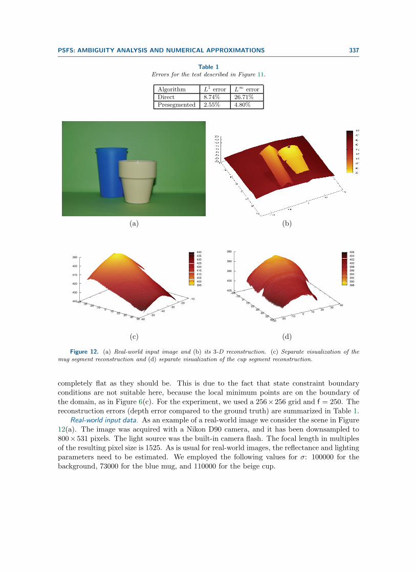
Real-world input data. As an example of a real-world image we consider the scene in Figure12(a). The image was acquired with a Nikon D90 camera, and it has been downsampled to800× 531 pixels. The light source was the built-in camera flash. The focal length in multiplesof the resulting pixel size is 1525. As is usual for real-world images, the reflectance and lightingparameters need to be estimated. We employed the following values for σ: 100000 for thebackground, 73000 for the blue mug, and 110000 for the beige cup.


The segment borders separating the cup from the mug as well as those separating thecup/mug from the background were obtained here by hand. They were enhanced a bit in orderto mask out points where interreflections between the objects were very strong. The specularhighlight at the upper lip of the cup was also masked out since such specular reflections are notincluded in the PSFS model. At the three resulting segments (subdomains)—cup, mug, andbackground—the PSFS equation was applied separately employing state constraint boundaryconditions.

Let us turn to the corresponding experimental result; see Figure 12(b). The general shapeof the objects and the background is captured in a rather accurate way. As expected, there isno tendency to enforce continuous transition between objects. This shows that the proposedidea of using state constraint boundary conditions at the borders of segmented objects worksproperly. Note that in the visualization of the whole scene together, the mug seems to havea wedge-like shape. This effect can be explained by specular highlights on the mug, which isnot handled in the PSFS model. In this visualization, however, the effect looks more drasticthan it actually is. To give a better impression on the shapes of the reconstruction, we alsoincluded separate visualizations of the mug and cup in Figures 12(c) and 12(d). The effect ofthe surface being pulled towards the optical center at specular highlights can also be observedin the reconstruction of the cup.

Concerning the quality of results, we observe some artifacts, as expected for this relativelydifficult real-world input image. The cup is reflected on the surface of the mug, and, inaddition, there are a lot of specular reflections as by the rough surface of the mug, so thatits reconstruction is drawn towards the camera. Both cup and mug are reflected on the greencardboard of the background, so that the latter is not reconstructed perfectly flat. We alsochose not to display the reconstruction of the ground on which the cup/mug are standing,since the absence of critical points there leads to a misinterpretation of the depth (as inthe synthetic input data test, local minimum points are on the boundary of the domain).Moreover, the quality of the reconstruction of the ground is degraded since the reflections ofboth the cup and the mug are strongly visible there.

Conclusion. In this paper, we have studied analytically and numerically the PSFS modeland the related Hamilton–Jacobi equation.

It turns out that ambiguities can still arise in the model as well as in practical computa-tions. If any knowledge of the true depth is available, it is impossible to reconstruct surfacessuch that

• they are not continuous (unless a presegmentation step is performed);• local minima are located at points of nondifferentiability;• local minima are located at the boundary.

We have also proved the convergence of a finite-difference scheme and a semi-Lagrangianscheme for the PSFS equation. In the latter case we employed an innovative technique forthe proof that can also be useful in contexts other than PSFS. Our theoretical results onthe numerics complement the analytical investigation of the ambiguity, ensuring that theambiguity issues are not due to numerical artifacts: ambiguities arise systematically even ifthe scheme in use converges to the viscosity solution of the equation.

Modern models like the PSFS studied here have a significant potential for applications.


We believe that this paper represents an important step towards a deeper understanding ofPSFS and other state-of-the-art SFS models, as well as towards the use of mathematicallyestablished numerical techniques in computer vision.

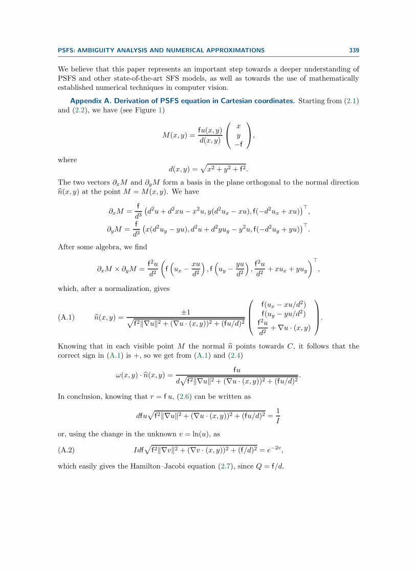
Appendix A. Derivation of PSFS equation in Cartesian coordinates. Starting from (2.1)and (2.2), we have (see Figure 1)

M(x, y) =fu(x, y)

d(x, y)

⎛⎝ xy−f

⎞⎠,

whered(x, y) =

√x2 + y2 + f2.

The two vectors ∂xM and ∂yM form a basis in the plane orthogonal to the normal directionn(x, y) at the point M = M(x, y). We have

∂xM =f

d3(d2u+ d2xu− x2u, y(d2ux − xu), f(−d2ux + xu)

)�,

∂yM =f

d3(x(d2uy − yu), d2u+ d2yuy − y2u, f(−d2uy + yu)

)�.

After some algebra, we find

∂xM × ∂yM =f2u

d2

(f(ux − xu

d2

), f(uy − yu

d2

),f2u

d2+ xux + yuy

)�,

which, after a normalization, gives

(A.1) n(x, y) =±1√

f2‖∇u‖2 + (∇u · (x, y))2 + (fu/d)2

⎛⎜⎜⎝f(ux − xu/d2)f(uy − yu/d2)

f2u

d2+∇u · (x, y)

⎞⎟⎟⎠.

Knowing that in each visible point M the normal n points towards C, it follows that thecorrect sign in (A.1) is +, so we get from (A.1) and (2.4)

ω(x, y) · n(x, y) = fu

d√

f2‖∇u‖2 + (∇u · (x, y))2 + (fu/d)2.

In conclusion, knowing that r = f u, (2.6) can be written as

dfu√

f2‖∇u‖2 + (∇u · (x, y))2 + (fu/d)2 =1

I

or, using the change in the unknown v = ln(u), as

(A.2) Idf√

f2‖∇v‖2 + (∇v · (x, y))2 + (f/d)2 = e−2v,

which easily gives the Hamilton–Jacobi equation (2.7), since Q = f/d.


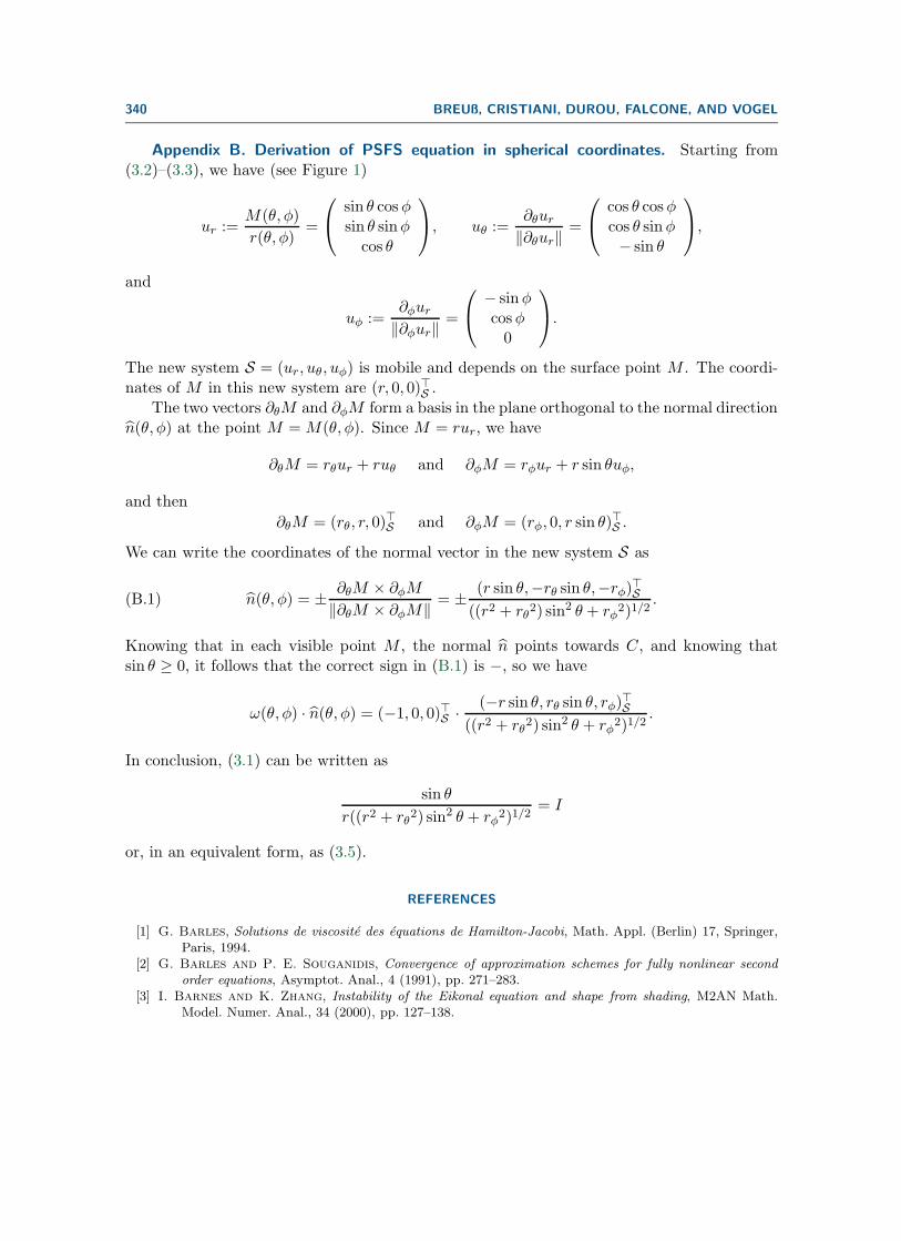
Appendix B. Derivation of PSFS equation in spherical coordinates. Starting from(3.2)–(3.3), we have (see Figure 1)

ur :=M(θ, φ)

r(θ, φ)=

⎛⎝ sin θ cosφsin θ sinφ

cos θ

⎞⎠, uθ :=∂θur

‖∂θur‖ =

⎛⎝ cos θ cosφcos θ sinφ− sin θ

⎞⎠,

and

uφ :=∂φur‖∂φur‖ =

⎛⎝ − sinφcosφ0

⎞⎠.

The new system S = (ur, uθ, uφ) is mobile and depends on the surface point M . The coordi-nates of M in this new system are (r, 0, 0)�S .

The two vectors ∂θM and ∂φM form a basis in the plane orthogonal to the normal directionn(θ, φ) at the point M = M(θ, φ). Since M = rur, we have

∂θM = rθur + ruθ and ∂φM = rφur + r sin θuφ,

and then

∂θM = (rθ, r, 0)�S and ∂φM = (rφ, 0, r sin θ)

�S .

We can write the coordinates of the normal vector in the new system S as

(B.1) n(θ, φ) = ± ∂θM × ∂φM

‖∂θM × ∂φM‖ = ± (r sin θ,−rθ sin θ,−rφ)�S

((r2 + rθ2) sin2 θ + rφ2)1/2

.

Knowing that in each visible point M , the normal n points towards C, and knowing thatsin θ ≥ 0, it follows that the correct sign in (B.1) is −, so we have

ω(θ, φ) · n(θ, φ) = (−1, 0, 0)�S · (−r sin θ, rθ sin θ, rφ)�S

((r2 + rθ2) sin2 θ + rφ2)1/2

.

In conclusion, (3.1) can be written as

sin θ

r((r2 + rθ2) sin2 θ + rφ2)1/2

= I

or, in an equivalent form, as (3.5).

REFERENCES

[1] G. Barles, Solutions de viscosite des equations de Hamilton-Jacobi, Math. Appl. (Berlin) 17, Springer,Paris, 1994.

[2] G. Barles and P. E. Souganidis, Convergence of approximation schemes for fully nonlinear secondorder equations, Asymptot. Anal., 4 (1991), pp. 271–283.

[3] I. Barnes and K. Zhang, Instability of the Eikonal equation and shape from shading, M2AN Math.Model. Numer. Anal., 34 (2000), pp. 127–138.


[4] A. Blake, A. Zisserman, and G. Knowles, Surface descriptions from stereo and shading, Image VisionComput., 3 (1985), pp. 183–191.

[5] M. Breuß, The implicit upwind method for 1-D scalar conservation laws with continuous fluxes, SIAMJ. Numer. Anal., 43 (2005), pp. 970–986.

[6] M. Breuß, E. Cristiani, J.-D. Durou, M. Falcone, and O. Vogel, Numerical algorithms forperspective shape from shading, Kybernetika (Prague), 46 (2010), pp. 207–225.

[7] M. J. Brooks, W. Chojnacki, and R. Kozera, Circularly symmetric Eikonal equations and non-uniqueness in computer vision, J. Math. Anal. Appl., 165 (1992), pp. 192–215.

[8] A. R. Bruss, The Eikonal equation: Some results applicable to computer vision, J. Math. Phys., 23(1982), pp. 890–896.

[9] F. Camilli and L. Grune, Numerical approximation of the maximal solutions for a class of degenerateHamilton-Jacobi equations, SIAM J. Numer. Anal., 38 (2000), pp. 1540–1560.

[10] F. Camilli and E. Prados, Viscosity solution, in Encyclopedia of Computer Vision, K. Ikeuchi, ed.,Springer, to appear.

[11] F. Courteille, A. Crouzil, J.-D. Durou, and P. Gurdjos, Towards shape from shading underrealistic photographic conditions, in Proceedings of the 17th International Conference on PatternRecognition, Vol. II, Cambridge, UK, 2004, pp. 277–280.

[12] F. Courteille, A. Crouzil, J.-D. Durou, and P. Gurdjos, Shape from shading for the digitizationof curved documents, Mach. Vision Appl., 18 (2007), pp. 301–316.

[13] E. Cristiani, Fast Marching and Semi-Lagrangian Methods for Hamilton-Jacobi Equations with Ap-plications, Ph.D. thesis, Dipartimento di Metodi e Modelli Matematici per le Scienze Applicate,SAPIENZA Universita di Roma, Rome, Italy, 2007.

[14] E. Cristiani, M. Falcone, and A. Seghini, Some remarks on perspective shape-from-shading models, inProceedings of the 1st International Conference on Scale Space and Variational Methods in ComputerVision (Ischia, Italy, 2007), F. Sgallari, A. Murli, and N. Paragios, eds., Lecture Notes in Comput.Sci. 4485, Springer-Verlag, Berlin, Heidelberg, 2007, pp. 276–287.

[15] P. Dupuis and J. Oliensis, An optimal control formulation and related numerical methods for a problemin shape reconstruction, Ann. Appl. Probab., 4 (1994), pp. 287–346.

[16] J.-D. Durou, M. Falcone, and M. Sagona, Numerical methods for shape-from-shading: A new surveywith benchmarks, Comput. Vis. Image Underst., 109 (2008), pp. 22–43.

[17] J.-D. Durou and D. Piau, Ambiguous shape from shading with critical points, J. Math. Imaging Vision,12 (2000), pp. 99–108.

[18] M. Falcone and R. Ferretti, Semi-Lagrangian Approximation Schemes for Linear and Hamilton–Jacobi Equations, SIAM, Philadelphia, to appear.

[19] M. Falcone and M. Sagona, An algorithm for the global solution of the shape-from-shading model, inImage Analysis and Processing, Lecture Notes in Comput. Sci. 1310, Springer, Berlin, Heidelberg,1997, pp. 596–603.

[20] B. K. P. Horn, Obtaining shape from shading information, in The Psychology of Computer Vision, P. H.Winston, ed., McGraw-Hill, New York, 1975, pp. 115–155.

[21] B. K. P. Horn, Robot Vision, MIT Press, Cambridge, MA, 1986.[22] B. K. P. Horn and M. J. Brooks, eds., Shape from Shading, MIT Press Ser. Artificial Intelligence,

MIT Press, Cambridge, MA, 1989.[23] R. Kimmel, K. Siddiqi, B. B. Kimia, and A. Bruckstein, Shape from shading: Level set propagation

and viscosity solutions, Int. J. Comput. Vision, 16 (1995), pp. 107–133.[24] P.-L. Lions, E. Rouy, and A. Tourin, Shape-from-shading, viscosity solutions and edges, Numer.

Math., 64 (1993), pp. 323–353.[25] T. Okatani and K. Deguchi, Shape reconstruction from an endoscope image by shape from shading

technique for a point light source at the projection center, Comput. Vis. Image Underst., 66 (1997),pp. 119–131.

[26] J. Oliensis, Uniqueness in shape from shading, Int. J. Comput. Vision, 6 (1991), pp. 75–104.[27] E. Prados, F. Camilli, and O. Faugeras, A unifying and rigorous shape from shading method adapted

to realistic data and applications, J. Math. Imaging Vision, 25 (2006), pp. 307–328.[28] E. Prados, F. Camilli, and O. Faugeras, A viscosity solution method for shape-from-shading without

image boundary data, M2AN Math. Model. Numer. Anal., 40 (2006), pp. 393–412.


[29] E. Prados and O. Faugeras, “Perspective shape from shading” and viscosity solutions, in Proceedingsof the Ninth IEEE International Conference on Computer Vision, Vol. 2, Nice, France, 2003, pp. 826–831.

[30] E. Prados and O. Faugeras, A generic and provably convergent shape-from-shading method for ortho-graphic and pinhole cameras, Int. J. Comput. Vision, 65 (2005), pp. 97–125.

[31] E. Prados and O. Faugeras, Shape from shading: A well-posed problem?, in Proceedings of the IEEEComputer Society Conference on Computer Vision and Pattern Recognition, Vol. 2, San Diego, CA,2005, pp. 870–877.

[32] E. Prados, O. Faugeras, and F. Camilli, Shape from Shading: A Well-Posed Problem?, Rapport deRecherche RR-5297, INRIA Sophia Antipolis, Sophia Antipolis, France, 2004.

[33] E. Rouy and A. Tourin, A viscosity solutions approach to shape-from-shading, SIAM J. Numer. Anal.,29 (1992), pp. 867–884.

[34] A. Tankus, N. Sochen, and Y. Yeshurun, A new perspective [on] shape-from-shading, in Proceedingsof the Ninth IEEE International Conference on Computer Vision, Vol. 2, Nice, France, 2003, pp. 862–869.

[35] A. Tankus, N. Sochen, and Y. Yeshurun, Perspective shape-from-shading by fast marching, in Pro-ceedings of the 2004 IEEE Computer Society Conference on Computer Vision and Pattern Recogni-tion, Vol. 1, Washington, DC, 2004, pp. 43–49.

[36] O. Vogel, M. Breuß, T. Leichtweis, and J. Weickert, Fast shape from shading for Phong-type sur-faces, in Proceedings of the Second International Conference on Scale Space and Variational Methodsin Computer Vision (Voss, Norway, 2009), X.-C. Tai, K. Mørken, M. Lysaker, and K.-A. Lie, eds.,Lecture Notes in Comput. Sci. 5567, Springer-Verlag, Berlin, Heidelberg, pp. 733–744.

[37] O. Vogel, M. Breuß, and J. Weickert, A direct numerical approach to perspective shape-from-shading, in Proceedings of the Vision, Modeling, and Visualization Conference 2007, VMW 2007,H. Lensch, B. Rosenhahn, H.-P. Seidel, P. Slusallek, and J. Weickert, eds., Saarbrucken, Germany,AKA, Berlin, 2007, pp. 91–100.

[38] R. Zhang, P.-S. Tsai, J. E. Cryer, and M. Shah, Shape from shading: A survey, IEEE Trans. PatternAnal. Mach. Intell., 21 (1999), pp. 690–706.

perspective shape from shading: ambiguity analysis and ... · perspective shape from shading:...

Documents