persistent atmospheric carbon dioxide biases in earth ... · 5/13/2014 · persistent atmospheric...
TRANSCRIPT

Persistent AtmosphericCarbon Dioxide Biasesin Earth SystemModels andCommunity ResearchDirectionsForrest M. Hoffman,James T. Randerson, Vivek K. Arora,Qing Bao, Patricia Cadule,Duoying Ji, Chris D. Jones,Michio Kawamiya, Samar Khatiwala,Keith Lindsay, Atsushi Obata,Elena Shevliakova, Katharina D. Six,Jerry F. Tjiputra, Evgeny M. Volodin,Tongwen Wu
DOE Integrated Climate ModelingPrincipal Investigator (PI) Meeting
May 13, 2014

Research Questions
Question 1
How well do Earth System Models (ESMs) simulate the observeddistribution of anthropogenic carbon in atmosphere, ocean, andland reservoirs?
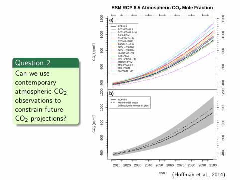
Question 2
Can we use contemporary atmospheric CO2 observations toconstrain future CO2 projections?

Research Questions
Question 1
How well do Earth System Models (ESMs) simulate the observeddistribution of anthropogenic carbon in atmosphere, ocean, andland reservoirs?
Question 2
Can we use contemporary atmospheric CO2 observations toconstrain future CO2 projections?

Observed Carbon Accumulation Since 1850
Year
Tota
l Car
bon
(Pg
C)
1850 1870 1890 1910 1930 1950 1970 1990 2010
0−
5050
150
250
350
0−
5050
150
250
350Anthropogenic Emissions (Andres et al., 2011, 2012)
Atmosphere (Meinshausen et al., 2011)Ocean (Khatiwala et al., 2013)Land (by difference)
Observational estimates of anthropogenic carbon inventories in atmosphere, ocean,and land reservoirs for 1850–2010. Atmosphere carbon is a fusion of Law Dome icecore CO2 observations, the Keeling Mauna Loa record, and more recently the NOAAGMD global surface average, integrated for the purpose of forcing IPCC models. Totalland flux is computed by mass balance as follows:
∆CL =∑i
Fi − ∆CA − ∆CO .

15 fully-prognostic ESMs that performed CMIP5emissions-forced simulations
Model Modeling Center
BCC-CSM1.1 Beijing Climate Center, ChinaMeteorological Administration, CHINA
BCC-CSM1.1(m) Beijing Climate Center, ChinaMeteorological Administration, CHINA
BNU-ESM Beijing Normal University, CHINACanESM2 Canadian Centre for Climate Modelling
and Analysis, CANADACESM1-BGC Community Earth System Model
Contributors, NSF-DOE-NCAR, USAFGOALS-s2.0 LASG, Institute of Atmospheric Physics,
CAS, CHINAGFDL-ESM2g NOAA Geophysical Fluid Dynamics
Laboratory, USAGFDL-ESM2m NOAA Geophysical Fluid Dynamics
Laboratory, USAHadGEM2-ES Met Office Hadley Centre, UNITED
KINGDOMINM-CM4 Institute for Numerical Mathematics,
RUSSIAIPSL-CM5A-LR Institut Pierre-Simon Laplace, FRANCE
MIROC-ESM Japan Agency for Marine-Earth Scienceand Technology, Atmosphere and OceanResearch Institute (University of Tokyo),and National Institute for EnvironmentalStudies, JAPAN
MPI-ESM-LR Max Planck Institute for Meteorology,GERMANY
MRI-ESM1 Meteorological Research Institute, JAPANNorESM1-ME Norwegian Climate Centre, NORWAY
CMIP5 Long-Term Experiments
Emissions for Historical + RCP 8.5 Simulations
Year
Ant
hrop
ogen
ic E
mis
sion
s (P
g C
/y)
1850 1900 1950 2000 2050 2100
05
1015
2025
30
05
1015
2025
30ESM HistoricalESM RCP 8.5

(a) Most ESMsexhibit a high bias inpredicted atmosphericCO2 mole fraction,which ranges from357–405 ppm at theend of the historicalperiod (1850–2005).
(b) The multi-modelmean is biased highfrom 1946 throughoutthe 20th century,ending 5.6 ppm abovethe observed value of378.8 ppm in 2005.
ESM Historical Atmospheric CO2 Mole Fraction
Year
CO
2 (pp
m)
280
300
320
340
360
380
400
420
280
300
320
340
360
380
400
420
ObservationsBCC−CSM1.1BCC−CSM1.1−MBNU−ESMCanESM2 (x3)CESM1−BGCFGOALS−s2.0GFDL−ESM2GGFDL−ESM2MHadGEM2−ESINM−CM4IPSL−CM5A−LRMIROC−ESMMPI−ESM−LR (x3)MRI−ESM1NorESM1−ME
a)
Year
CO
2 (pp
m)
1850 1870 1890 1910 1930 1950 1970 1990 2010
280
300
320
340
360
380
400
420
280
300
320
340
360
380
400
420
ObservationsMulti−model Mean(with range/envelope in grey)
b)
(Hoffman et al., 2014)
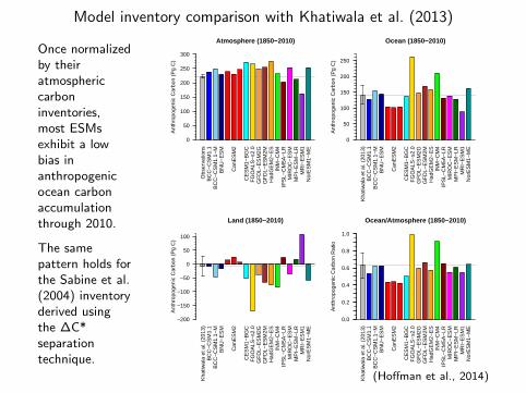
Model inventory comparison with Khatiwala et al. (2013)
Once normalizedby theiratmosphericcarboninventories,most ESMsexhibit a lowbias inanthropogenicocean carbonaccumulationthrough 2010.
The samepattern holds forthe Sabine et al.(2004) inventoryderived usingthe ∆C*separationtechnique.
Obs
erva
tions
BC
C−
CS
M1.
1B
CC
−C
SM
1.1−
MB
NU
−E
SM
Can
ES
M2
CE
SM
1−B
GC
FG
OA
LS−
s2.0
GF
DL−
ES
M2G
GF
DL−
ES
M2M
Had
GE
M2−
ES
INM
−C
M4
IPS
L−C
M5A
−LR
MIR
OC
−E
SM
MP
I−E
SM
−LR
MR
I−E
SM
1N
orE
SM
1−M
E
Atmosphere (1850−2010)
Ant
hrop
ogen
ic C
arbo
n (P
g C
)
0
50
100
150
200
250
300
Kha
tiwal
a et
al.
(201
3)B
CC
−C
SM
1.1
BC
C−
CS
M1.
1−M
BN
U−
ES
M
Can
ES
M2
CE
SM
1−B
GC
FG
OA
LS−
s2.0
GF
DL−
ES
M2G
GF
DL−
ES
M2M
Had
GE
M2−
ES
INM
−C
M4
IPS
L−C
M5A
−LR
MIR
OC
−E
SM
MP
I−E
SM
−LR
MR
I−E
SM
1N
orE
SM
1−M
E
Ocean (1850−2010)
Ant
hrop
ogen
ic C
arbo
n (P
g C
)
0
50
100
150
200
250
Kha
tiwal
a et
al.
(201
3)B
CC
−C
SM
1.1
BC
C−
CS
M1.
1−M
BN
U−
ES
M
Can
ES
M2
CE
SM
1−B
GC
FG
OA
LS−
s2.0
GF
DL−
ES
M2G
GF
DL−
ES
M2M
Had
GE
M2−
ES
INM
−C
M4
IPS
L−C
M5A
−LR
MIR
OC
−E
SM
MP
I−E
SM
−LR
MR
I−E
SM
1N
orE
SM
1−M
E
Land (1850−2010)
Ant
hrop
ogen
ic C
arbo
n (P
g C
)
−200
−150
−100
−50
0
50
100
Kha
tiwal
a et
al.
(201
3)B
CC
−C
SM
1.1
BC
C−
CS
M1.
1−M
BN
U−
ES
M
Can
ES
M2
CE
SM
1−B
GC
FG
OA
LS−
s2.0
GF
DL−
ES
M2G
GF
DL−
ES
M2M
Had
GE
M2−
ES
INM
−C
M4
IPS
L−C
M5A
−LR
MIR
OC
−E
SM
MP
I−E
SM
−LR
MR
I−E
SM
1N
orE
SM
1−M
E
Ocean/Atmosphere (1850−2010)
Ant
hrop
ogen
ic C
arbo
n R
atio
0.0
0.2
0.4
0.6
0.8
1.0
(Hoffman et al., 2014)

(a) Ocean inventoryestimates have afairly persistentordering during thesecond half of the20th century.
(b) ESMs have awide range of landcarbon accumulationresponses toincreasing CO2 andland use change,ranging from a netsource of 170 Pg C toa sink of 107 Pg C in2010.
ESM Historical Ocean and Land Carbon Accumulation
Year
Oce
an C
Acc
umul
atio
n (P
g C
)
050
100
150
200
250
050
100
150
200
250
ObservationsBCC−CSM1.1BCC−CSM1.1−MBNU−ESM (units corrected)CanESM2 (x3) (units corrected)CESM1−BGCFGOALS−s2.0GFDL−ESM2GGFDL−ESM2MHadGEM2−ESINM−CM4IPSL−CM5A−LRMIROC−ESMMPI−ESM−LR (x3)MRI−ESM1 (units corrected)NorESM1−ME
a)
Year
Land
C A
ccum
ulat
ion
(Pg
C)
1850 1870 1890 1910 1930 1950 1970 1990 2010
−17
5−
125
−75
−25
2575
−17
5−
125
−75
−25
2575
b)
(Hoffman et al., 2014)
Question 2
Can we usecontemporaryatmospheric CO2
observations toconstrain futureCO2 projections?
ESM RCP 8.5 Atmospheric CO2 Mole Fraction
Year
CO
2 (pp
m)
400
600
800
1000
1200
400
600
800
1000
1200
RCP 8.5BCC−CSM1.1BCC−CSM1.1−MBNU−ESMCanESM2 (x3)CESM1−BGCFGOALS−s2.0GFDL−ESM2GGFDL−ESM2MHadGEM2−ESINM−CM4IPSL−CM5A−LRMIROC−ESMMPI−ESM−LRMRI−ESM1NorESM1−ME
a)
Year
CO
2 (pp
m)
2010 2020 2030 2040 2050 2060 2070 2080 2090 2100
400
600
800
1000
1200
400
600
800
1000
1200
RCP 8.5Multi−model Mean(with range/envelope in grey)
b)
(Hoffman et al., 2014)

Reducing Uncertainties Using Observations
To reduce feedback uncertainties using contemporary observations,
1. there must be a relationship between contemporary variabilityand future trends on longer time scales within the model, and
2. it must be possible to constrain contemporary variability inthe model using observations.
Example #1
Hall and Qu (2006) evaluated thestrength of the springtime snowalbedo feedback (SAF; ∆αs/∆Ts)from 17 models used for the IPCCAR4 and compared them with theobserved springtime SAF fromISCCP and ERA-40 reanalysis.

Reducing Uncertainties Using Observations
To reduce feedback uncertainties using contemporary observations,
1. there must be a relationship between contemporary variabilityand future trends on longer time scales within the model, and
2. it must be possible to constrain contemporary variability inthe model using observations.
Example #2
Cox et al. (2013) used the observedrelationship between the CO2 growthrate and tropical temperature as aconstraint to reduce uncertainty inthe land carbon storage sensitivity toclimate change (γL) in the tropicsusing C4MIP models.

We developed a newemergent constraintfrom carboninventories.
A relationship existsbetweencontemporary andfuture atmosphericCO2 levels overdecadal time scalesbecause carbon modelbiases persist overdecadal time scales.
Observed contemporaryatmospheric CO2 molefraction is represented bythe vertical line at384.6 ± 0.5 ppm.
(Hoffman et al., 2014)
Future vs. Contemporary Atmospheric CO2 Mole Fraction
0
Fut
ure
(206
0) C
O2 M
ole
Fra
ctio
n (p
pm)
500
550
600
650
700
750
500
550
600
650
700
750
Observations
Historical + RCP8.5BCC−CSM1.1BCC−CSM1.1−MBNU−ESMCanESM2 (x3)CESM1−BGCFGOALS−s2.0GFDL−ESM2GGFDL−ESM2MHadGEM2−ESINM−CM4IPSL−CM5A−LRMIROC−ESMMPI−ESM−LRMRI−ESM1NorESM1−ME
a) 2060
R2 = 0.70
Contemporary (2010) CO2 Mole Fraction (ppm)
Fut
ure
(210
0) C
O2 M
ole
Fra
ctio
n (p
pm)
360 365 370 375 380 385 390 395 400 405 410
700
800
900
1000
1100
700
800
900
1000
1100
b) 2100
R2 = 0.54

R2 of Multi−model Bias Structure
Year
R2
1850 1875 1900 1925 1950 1975 2000 2025 2050 2075 2100
0.0
0.2
0.4
0.6
0.8
1.0
0.0
0.2
0.4
0.6
0.8
1.0
R2 = 0.23, N = 17, p < 0.05
OceanLandAtmosphere
(Hoffman et al., 2014)
The coefficients of determination (R2) of the multi-model bias structurerelative to the set of CMIP5 model atmospheric CO2, and ocean and landcarbon predictions for 2010 are statistically significant for 1910–2100.

Contemporary CO2 Tuned Model (CCTM)
Year
CO
2 (pp
m)
1850 1875 1900 1925 1950 1975 2000 2025 2050 2075 2100
300
500
700
900
1100
300
500
700
900
1100Observations
RCP 8.5Multi−Model Mean and95th percentile rangeCCTM and95% confidence interval
We used this regression to create acontemporary CO2 tuned model(CCTM) estimate of the atmosphericCO2 trajectory for the 21st century.
The width of the probability densityis much smaller for the CCTM, byalmost a factor of 6 at 2060 andalmost a factor of 5 at 2100,indicating a significant reduction inthe range of uncertainty for theCCTM prediction.
Probability Density of Atmospheric CO2 Mole Fraction
CO2 Mole Fraction (ppm)
Den
sity
520 540 560 580 600 620 640 660 680 700
0.00
0.02
0.04
0.06
02
4
Fre
quen
cy
Multi−model PDMulti−model MeanCCTM PDCCTM Prediction
a) 2060
CO2 Mole Fraction (ppm)D
ensi
ty
750 800 850 900 950 1000 1050 1100 1150
0.00
00.
005
0.01
00.
015
0.02
00.
025
02
46
Fre
quen
cy
b) 2100
Best estimate tuned using Mauna LoaCO2 data:
At 2060: 600 ± 14 ppm, 21 ppm belowthe multi-model mean
At 2100: 947 ± 35 ppm, 32 ppm belowthe multi-model mean
(Hoffman et al., 2014)

Projections for Individual CMIP5 Models
Year
Rad
iativ
e F
orci
ng (W
m−2
)
01
23
45
67 Observations
RCP 8.5BCC−CSM1.1BCC−CSM1.1−MBNU−ESMCanESM2 (x3)CESM1(BGC)FGOALS−s2.0GFDL−ESM2GGFDL−ESM2MHadGEM2−ESINM−CM4IPSL−CM5A−LRMIROC−ESMMPI−ESM−LRMRI−ESM1NorESM1−ME
a) Radiative Forcing
CCTM Relative to the Multi − Model Mean
Year
Rad
iativ
e F
orci
ng (W
m−2
)
01
23
45
67Observations
RCP 8.5Multi−Model Mean and95th percentile rangeCCTM and95% confidence interval
b) Radiative Forcing
Year
∆T (°
C)
1850 1875 1900 1925 1950 1975 2000 2025 2050 2075 2100
01
23
45 c) Temperature Change
Year
∆T (K
)
1850 1875 1900 1925 1950 1975 2000 2025 2050 2075 2100
01
23
45d) Temperature Change
(Hoffman et al., 2014)
We calculated the CO2 radiative forcing and used an impulse response function(tuned to the mean transient climate response of CMIP5 models) to equitablycompute the resulting temperature change for models and the CCTM. At 2100,the CCTM ∆T = 4.0 ± 0.1◦C, while the multi-model mean ∆T = 4.2 ± 0.6◦C.

Future vs. Contemporary Ocean Accumulation
0
Fut
ure
(206
0) O
cean
Acc
umul
atio
n (P
g C
)
200
300
400
500
600
Observations
BCC−CSM1.1BCC−CSM1.1−MBNU−ESMCanESM2 (x3)CESM1−BGCFGOALS−s2.0GFDL−ESM2GGFDL−ESM2MHadGEM2−ESINM−CM4IPSL−CM5A−LRMIROC−ESMMPI−ESM−LRMRI−ESM1NorESM1−ME
a) 2060
R2 = 0.95
Future vs. Contemporary Land Accumulation
0
0
−30
0−
100
010
020
030
040
0
Fut
ure
(206
0) L
and
Acc
umul
atio
n (P
g C
)
Observationsb) 2060
R2 = 0.82
Contemporary (2010) Ocean Accumulation (Pg C)
Fut
ure
(210
0) O
cean
Acc
umul
atio
n (P
g C
)
70 90 110 130 150 170 190 210 230 250
300
400
500
600
700
800
900
c) 2100
R2 = 0.92
Contemporary (2010) Land Accumulation (Pg C)
0
−180 −140 −100 −60 −20 0 20 40 60 80
−50
0−
200
020
040
060
080
0
Fut
ure
(210
0) L
and
Acc
umul
atio
n (P
g C
)d) 2100
R2 = 0.70
(Hoffman et al., 2014)
We also developed a multi-model constraint on the evolution of oceanand land anthropogenic inventories. Since observational uncertainties arehigher for ocean and land, uncertainties in future estimates cannot bereduced as much as for atmospheric CO2.

Conclusions
I A considerable amount of the model-to-model variability of CO2 inthe 21st century can be traced to biases that exist at the end of theobservational record.
I Bias persistence was highest for the ocean, followed by land, andthen by the atmosphere.
I Carbon cycle biases are likely primarily linked withconcentration–carbon feedback processes:
I ocean – Southern Ocean overturning, vertical mixing processesI land – CO2 fertilization, allocation to woody pools, nutrient
limitation
I Future fossil fuel emissions targets designed to stabilize CO2 levelswould be too low if estimated from the multi-model mean of ESMs.
I ESMs overestimate contemporary CO2 with observed emissions.
I Models could be improved through extensive comparison withobservations and community model benchmarking.
For more information, see also Poster #77 in Room 20

I We co-organized inaugural meeting and ∼45 researchers participatedfrom the United States, Canada, the United Kingdom, the Netherlands,France, Germany, Switzerland, China, Japan, and Australia.
I ILAMB Goals: Develop internationally accepted benchmarks for modelperformance, advocate for design of open-source software system, andstrengthen linkages between experimental, monitoring, remote sensing,and climate modeling communities. Initial focus on CMIP5 models.
I Provides methodology for model–data comparison and baseline standardfor performance of land model process representations (Luo et al., 2012).

ILAMB 1.0 Benchmarks Now Under Development
Annual Seasonal InterannualMean Cycle Variability Trend Data Source
Atmospheric CO2Flask/conc. + transport X X X NOAA, SIO, CSIRO
TCCON + transport X X X CaltechFluxnet
GPP, NEE, TER, LE, H, RN X X X Fluxnet, MAST-DCGridded: GPP X X ? MPI-BGC
Hydrology/Energyrunoff ratio (R/P) river flow X X GRDC, Dai, GFDL
global runoff/ocean balance X Syed/Famigliettialbedo (multi-band) X X MODIS, CERES
soil moisture X X de Jeur, SMAPcolumn water X X GRACE
snow cover X X X X AVHRR, GlobSnowsnow depth/SWE X X X X CMC (N. America)
Tair & P X X X X CRU, GPCP and TRMMGridded: LE, H X X MPI-BGC, dedicated ET
Ecosystem Processes & Statesoil C, N X HWSD, MPI-BGC
litter C, N X LIDETsoil respiration X X X X Bond-Lamberty
FAPAR X X MODIS, SeaWIFSbiomass & change X X Saatchi, Pan, Blackard
canopy height X Lefsky, FisherNPP X EMDI, Luyssaert
Vegetation Dynamicsfire — burned area X X X GFED3
wood harvest X X Hurttland cover X MODIS PFT fraction

Example Benchmark Score Sheet from C-LAMP
Models
BG
C D
atasets
Uncertainty Scaling TotalMetric Metric components of obs. mismatch score Sub-score CASA′ CN
LAI Matching MODIS observations 15.0 13.5 12.0• Phase (assessed using the month of maximum LAI) Low Low 6.0 5.1 4.2• Maximum (derived separately for major biome classes) Moderate Low 5.0 4.6 4.3• Mean (derived separately for major biome classes) Moderate Low 4.0 3.8 3.5
NPP Comparisons with field observations and satellite products 10.0 8.0 8.2• Matching EMDI Net Primary Production observations High High 2.0 1.5 1.6• EMDI comparison, normalized by precipitation Moderate Moderate 4.0 3.0 3.4• Correlation with MODIS (r2) High Low 2.0 1.6 1.4• Latitudinal profile comparison with MODIS (r2) High Low 2.0 1.9 1.8
CO2 annual cycle Matching phase and amplitude at Globalview flash sites 15.0 10.4 7.7• 60◦–90◦N Low Low 6.0 4.1 2.8• 30◦–60◦N Low Low 6.0 4.2 3.2• 0◦–30◦N Moderate Low 3.0 2.1 1.7
Energy & CO2 fluxes Matching eddy covariance monthly mean observations 30.0 17.2 16.6• Net ecosystem exchange Low High 6.0 2.5 2.1• Gross primary production Moderate Moderate 6.0 3.4 3.5• Latent heat Low Moderate 9.0 6.4 6.4• Sensible heat Low Moderate 9.0 4.9 4.6
Transient dynamics Evaluating model processes that regulate carbon exchange 30.0 16.8 13.8on decadal to century timescales• Aboveground live biomass within the Amazon Basin Moderate Moderate 10.0 5.3 5.0• Sensitivity of NPP to elevated levels of CO2: comparison Low Moderate 10.0 7.9 4.1
to temperate forest FACE sites• Interannual variability of global carbon fluxes: High Low 5.0 3.6 3.0
comparison with TRANSCOM• Regional and global fire emissions: comparison to High Low 5.0 0.0 1.7
GFEDv2Total: 100.0 65.9 58.3
(Randerson et al., 2009)

10 Alaska Ecoregions, Present and Future
1000 km 1000 km
2000–2009 2090–2099(Hoffman et al., 2013)
Since the random colors are the same in both maps, a change incolor represents an environmental change between the present andthe future.At this level of division, the conditions in the large boreal forestbecome compressed onto the Brooks Range and the conditions onthe Seward Peninsula “migrate” to the North Slope.

Present Representativeness of Barrow or “Barrow-ness”
1000 km
(Hoffman et al., 2013)
Light-colored regions are well represented and dark-colored regionsare poorly represented by the sampling location listed in red.
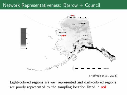
Network Representativeness: Barrow + Council
1000 km
(Hoffman et al., 2013)
Light-colored regions are well represented and dark-colored regionsare poorly represented by the sampling location listed in red.

Barrow Environmental Observatory (BEO)
(Kumar et al., in prep)
Representativeness map for vegetation sampling points for A, B, C,and D sampling area (left) and zoomed in on the C samping area(right) developed from WorldView2 satellite images for the year2010 and LiDAR data.
Vegetation sampling locations represent polygon troughs (red),edges (green), and centers (blue).

(a) dry tundra gramanoid (b) forb
(c) lichen (d) moss(Kumar et al., in prep)
Example plant functional type (PFT) distributions scaled up fromvegetation sampling locations.

Triple-network Global Representativeness
(Maddalena et al., in prep)
Map indicates which sampling network offers the mostrepresentative coverage at any location. Every location is made upof a combination of three primary colors from Fluxnet (red),ForestGEO (green), and RAINFOR (blue).

CESD Mission – My view
Data and ModelsCommunity
for site selection
& network analysis
site characterization
experimental design
and
sampling strategy
field measurements
and manipulative
experiments
data synthesis,
scaling, and
integration
modular design
employing
model development
model experiments
model evaluation
and
sensitivity analysis
knowledge gaps
of key
identification
designed to test
functional responses
ILAMB
CMIP6
Earth system grid
modeling centers
ARM archive
literaturedata centers
synthesis groups
RGCM
ESM
ASRTES
SBR
DM

Biogeochemistry–Climate System Feedbacks
comparisonsModel
experimentsSensitivity
campaignsMeasurement Manipulation
experiments sensingRemote
Measurements & Experiments Community
for Understanding Fundamental Processes
Earth System Modeling Community
for Predicting Impacts of Environmental Change
AmeriFlux
TestbedsModel
Modelinggroups
BenchmarkingPackage
EarthSystem
GridFederation
Biogeochemistry−Climate
Feedbacks SFA
Ne
w m
od
el
imp
rov
em
en
tsN
ew
me
as
ure
me
nt
ca
mp
aig
ns

Take Home Message from Bruce and Forrest
I Modelers: Confront models with data. Just like voting, dothis early and often!
I Make model evaluation tools and data free and open,facilitating community contributions. It takes a village!
I Design model experiments and analyses to identify weaknessesand inspire new measurements.
I Data Gatherers: Make data available early and characterizeand report all measurement uncertainties.
I Confront the environment with new sensors, drones, and aerialand space-based instrumentation to answer key questionsabout mechanisms.
I Conduct measurements to improve our understanding ofprocesses and inform model development.
I Integrated Assessors: Creatively employ multi-modelprojections and use results of model evalutaion as a lensthrough which to view predictions of the future.

Acknowledgments
This research was sponsored by the Climate and Environmental SciencesDivision (CESD) of the Biological and Environmental Research (BER) Programin the U. S. Department of Energy Office of Science and the National ScienceFoundation (AGS-1048890). This research used resources of the NationalCenter for Computational Sciences (NCCS) at Oak Ridge National Laboratory(ORNL), which is managed by UT-Battelle, LLC, for the U. S. Department ofEnergy under Contract No. DE-AC05-00OR22725.
We acknowledge the World Climate Research Programme’s Working Group onCoupled Modelling, which is responsible for CMIP, and we thank the climatemodeling groups for producing and making available their model output. ForCMIP the U. S. Department of Energy’s Program for Climate Model Diagnosisand Intercomparison provides coordinating support and led development ofsoftware infrastructure in partnership with the Global Organization for EarthSystem Science Portals.

ReferencesR. J. Andres, J. S. Gregg, L. Losey, G. Marland, and T. A. Boden. Monthly, global emissions of carbon dioxide from
fossil fuel consumption. Tellus B, 63(3):309–327, July 2011. doi: 10.1111/j.1600-0889.2011.00530.x.
P. M. Cox, D. Pearson, B. B. Booth, P. Friedlingstein, C. Huntingford, C. D. Jones, and C. M. Luke. Sensitivity oftropical carbon to climate change constrained by carbon dioxide variability. Nature, 494(7437):341–344, Feb.2013. doi: 10.1038/nature11882.
A. Hall and X. Qu. Using the current seasonal cycle to constrain snow albedo feedback in future climate change.Geophys. Res. Lett., 33(3):L03502, Feb. 2006. doi: 10.1029/2005GL025127.
F. M. Hoffman, J. Kumar, R. T. Mills, and W. W. Hargrove. Representativeness-based sampling network design forthe State of Alaska. Landscape Ecol., 28(8):1567–1586, Oct. 2013. doi: 10.1007/s10980-013-9902-0.
F. M. Hoffman, J. T. Randerson, V. K. Arora, Q. Bao, P. Cadule, D. Ji, C. D. Jones, M. Kawamiya, S. Khatiwala,K. Lindsay, A. Obata, E. Shevliakova, K. D. Six, J. F. Tjiputra, E. M. Volodin, and T. Wu. Causes andimplications of persistent atmospheric carbon dioxide biases in Earth System Models. J. Geophys. Res.Biogeosci., 119(2):141–162, Feb. 2014. doi: 10.1002/2013JG002381.
S. Khatiwala, T. Tanhua, S. Mikaloff Fletcher, M. Gerber, S. C. Doney, H. D. Graven, N. Gruber, G. A. McKinley,A. Murata, A. F. Rıos, and C. L. Sabine. Global ocean storage of anthropogenic carbon. Biogeosci., 10(4):2169–2191, Apr. 2013. doi: 10.5194/bg-10-2169-2013.
Y. Q. Luo, J. T. Randerson, G. Abramowitz, C. Bacour, E. Blyth, N. Carvalhais, P. Ciais, D. Dalmonech, J. B.Fisher, R. Fisher, P. Friedlingstein, K. Hibbard, F. Hoffman, D. Huntzinger, C. D. Jones, C. Koven,D. Lawrence, D. J. Li, M. Mahecha, S. L. Niu, R. Norby, S. L. Piao, X. Qi, P. Peylin, I. C. Prentice, W. Riley,M. Reichstein, C. Schwalm, Y. P. Wang, J. Y. Xia, S. Zaehle, and X. H. Zhou. A framework for benchmarkingland models. Biogeosci., 9(10):3857–3874, Oct. 2012. doi: 10.5194/bg-9-3857-2012.
M. Meinshausen, S. Smith, K. Calvin, J. Daniel, M. Kainuma, J.-F. Lamarque, K. Matsumoto, S. Montzka,S. Raper, K. Riahi, A. Thomson, G. Velders, and D. P. van Vuuren. The RCP greenhouse gas concentrationsand their extensions from 1765 to 2300. Clim. Change, 109(1):213–241, Nov. 2011. doi:10.1007/s10584-011-0156-z.
J. T. Randerson, F. M. Hoffman, P. E. Thornton, N. M. Mahowald, K. Lindsay, Y.-H. Lee, C. D. Nevison, S. C.Doney, G. Bonan, R. Stockli, C. Covey, S. W. Running, and I. Y. Fung. Systematic assessment of terrestrialbiogeochemistry in coupled climate-carbon models. Global Change Biol., 15(9):2462–2484, Sept. 2009. doi:10.1111/j.1365-2486.2009.01912.x.
C. L. Sabine, R. A. Feely, N. Gruber, R. M. Key, K. Lee, J. L. Bullister, R. Wanninkhof, C. S. Wong, D. W. R.Wallace, B. Tilbrook, F. J. Millero, T.-H. Peng, A. Kozyr, T. Ono, and A. F. Rios. The oceanic sink foranthropogenic CO2. Science, 305(5682):367–371, July 2004. doi: 10.1126/science.1097403.

Extra Slides

Model inventory comparison with Sabine et al. (2004)
Obs
erva
tions
BC
C−
CS
M1.
1B
CC
−C
SM
1.1−
MB
NU
−E
SM
Can
ES
M2
CE
SM
1−B
GC
FG
OA
LS−
s2.0
GF
DL−
ES
M2G
GF
DL−
ES
M2M
Had
GE
M2−
ES
INM
−C
M4
IPS
L−C
M5A
−LR
MIR
OC
−E
SM
MP
I−E
SM
−LR
MR
I−E
SM
1N
orE
SM
1−M
E
Atmosphere (1850−1994)
Ant
hrop
ogen
ic C
arbo
n (P
g C
)
0
50
100
150
200
250
300
Sab
ine
et a
l. (2
004)
BC
C−
CS
M1.
1B
CC
−C
SM
1.1−
MB
NU
−E
SM
Can
ES
M2
CE
SM
1−B
GC
FG
OA
LS−
s2.0
GF
DL−
ES
M2G
GF
DL−
ES
M2M
Had
GE
M2−
ES
INM
−C
M4
IPS
L−C
M5A
−LR
MIR
OC
−E
SM
MP
I−E
SM
−LR
MR
I−E
SM
1N
orE
SM
1−M
E
Ocean (1850−1994)
Ant
hrop
ogen
ic C
arbo
n (P
g C
)
0
50
100
150
200
250
Sab
ine
et a
l. (2
004)
BC
C−
CS
M1.
1B
CC
−C
SM
1.1−
MB
NU
−E
SM
Can
ES
M2
CE
SM
1−B
GC
FG
OA
LS−
s2.0
GF
DL−
ES
M2G
GF
DL−
ES
M2M
Had
GE
M2−
ES
INM
−C
M4
IPS
L−C
M5A
−LR
MIR
OC
−E
SM
MP
I−E
SM
−LR
MR
I−E
SM
1N
orE
SM
1−M
E
Land (1850−1994)
Ant
hrop
ogen
ic C
arbo
n (P
g C
)
−200
−150
−100
−50
0
50
100
Sab
ine
et a
l. (2
004)
BC
C−
CS
M1.
1B
CC
−C
SM
1.1−
MB
NU
−E
SM
Can
ES
M2
CE
SM
1−B
GC
FG
OA
LS−
s2.0
GF
DL−
ES
M2G
GF
DL−
ES
M2M
Had
GE
M2−
ES
INM
−C
M4
IPS
L−C
M5A
−LR
MIR
OC
−E
SM
MP
I−E
SM
−LR
MR
I−E
SM
1N
orE
SM
1−M
E
Ocean/Atmosphere (1850−1994)
Ant
hrop
ogen
ic C
arbo
n R
atio
0.0
0.2
0.4
0.6
0.8
1.0

Implications for CO2, Radiative Forcing, and Temperature
CO2 Mole Radiative Cumulative ∆TFraction (ppm) Forcing (W m−2) ∆T (◦C) Bias (◦C)
Model 2010 2060 2100 2010 2060 2100 2010 2060 2100 2010 2060 2100
BCC-CSM1.1 390 603 945 1.70 4.03 6.43 0.97 2.39 4.02 0.03 0.02 −0.01BCC-CSM1.1-M 396 619 985 1.78 4.16 6.65 1.04 2.49 4.16 0.10 0.12 0.13
BNU-ESM 382 602 963 1.59 4.02 6.53 0.90 2.33 4.07 −0.04 −0.04 0.04CanESM2 r1 394 641 1024 1.75 4.36 6.86 0.98 2.58 4.30 0.04 0.21 0.27CanESM2 r2 392 641 1023 1.72 4.35 6.85 0.98 2.57 4.30 0.04 0.20 0.27CanESM2 r3 396 641 1025 1.78 4.35 6.87 1.01 2.58 4.30 0.07 0.21 0.27CESM1-BGC 407 697 1121 1.92 4.80 7.34 1.12 2.85 4.64 0.18 0.48 0.61FGOALS-s2.0 404 636 993 1.89 4.31 6.70 1.09 2.57 4.23 0.15 0.20 0.20GFDL-ESM2G 395 616 967 1.77 4.14 6.56 1.04 2.49 4.12 0.10 0.12 0.09GFDL-ESM2M 400 621 964 1.83 4.18 6.54 1.09 2.52 4.13 0.15 0.15 0.10HadGEM2-ES 411 636 983 1.98 4.31 6.64 1.18 2.60 4.20 0.24 0.23 0.17
INM-CM4 386 591 897 1.64 3.92 6.15 0.92 2.36 3.86 −0.02 −0.01 −0.17IPSL-CM5A-LR 375 573 908 1.48 3.75 6.22 0.86 2.21 3.87 −0.08 −0.16 −0.16
MIROC-ESM 398 658 1121 1.81 4.50 7.35 1.06 2.67 4.58 0.12 0.30 0.55MPI-ESM-LR r1 383 590 948 1.60 3.91 6.45 0.95 2.31 4.03 0.01 −0.06 0.00
MRI-ESM1 361 516 778 1.28 3.20 5.39 0.74 1.89 3.33 −0.20 −0.48 −0.70NorESM1-ME 391 667 1070 1.72 4.57 7.09 0.98 2.68 4.46 0.04 0.31 0.43
Multi-model Mean 392 621 980 1.72 4.18 6.63 1.00 2.48 4.17 0.06 0.11 0.14CCTM Estimate 385 600 948 1.62 4.01 6.45 0.94 2.37 4.03 — — —
Historical + RCP 8.5 385 590 917 1.63 3.91 6.27 0.94 2.32 3.93 0.00 −0.05 −0.10