Performance Test for GeosyntheticReinforced Soil Including Effects of PreloadingFHWA-RD-01-118 JUNE 2001

Research, Development, and TechnologyTurner-Fairbank Highway Research Center6300 Georgetown PikeMcLean, VA 22101-2296

FOREWORD

Geosynthetic reinforced soil (GRS) systems were tested under different loading conditions in order to develop a simplified model for predicting the deformation characteristics of a GRS mass. A simplified preloading-reloading (SPR) analytical model was developed to predict the deformation characteristics of GRS masses subject to monotonic loading and preloading/loading. The SPR model was shown to be able to accurately predict the results obtained from a revised laboratory performance test. The results of this study will be of interest and utility to geotechnologists working with GRS systems.

T. Paul Teng, P. E. Director, Office of Infrastructure, Research and Development

NOTICE

This document is disseminated under the sponsorship of the Department of Transportation in the interest of information exchange. The United States Government assumes no liability for its contents thereof. This report does not constitute a standard, specification, or regulation. The United States Government does not endorse products or manufacturers. Trademarks or manufacturer’s names appear herein only because they are considered essential to the object of this document.

Technical Report Documentation Page 1. Report No. FHWA-RD-01-018

2. Government Accession No.

3. Recipient's Catalog No.

5. Report Date June 2001

4. Title and Subtitle PERFORMANCE TEST FOR GEOSYNTHETIC-REINFORCED SOIL INCLUDING EFFECTS OF PRELOADING

6. Performing Organization Code

7. Author(s) Kanop Ketchart and Jonathan T.H. Wu

8. Performing Organization Report No.

10. Work Unit No. (TRAIS)

9. Performing Organization Name and Address Reinforced Soil Research Center University of Colorado at Denver 1200 Larimer Street Denver, CO 80217-3364

11. Contract or Grant No. DTFH61-98-P-00402 13. Type of Report and Period Covered

12. Sponsoring Agency Name and Address Office of Infrastructure R&D Federal Highway Administration 6300 Georgetown Pike McLean, VA 22101-2296

14. Sponsoring Agency Code

15. Supplementary Notes Contracting Officer's Technical Representative (COTR): M.T. Adams 16. Abstract A study was undertaken to investigate the behavior of Geosynthetic Reinforced Soil (GRS) masses under various loading conditions and to develop a simplified analytical model for predicting deformation characteristics of a generic GRS mass. Significant emphasis was placed on the effect of preloading. To conduct the study, a revised laboratory test, known as the Soil-Geosynthetic Performance (SGP) test, was first developed. The test is capable of investigating the behavior of a generic GRS mass in a manner mimicking the field placement condition, and the soil and geosynthetic reinforcement are allowed to deform in an interactive manner. A series of SGP tests was performed. Different soils and reinforcements were employed, and the soil-geosynthetic composites were subject to various loading sequences. The tests showed that preloading typically reduces vertical and lateral deformations of a generic soil mass by a factor 2 to 7, and that prestressing (preloading followed by reloading from a non-zero stress level) can further increase the vertical stiffness by a factor of 2 to 2.5. Correlations between the results of SGP tests and full-scale GRS structures were evaluated. It was found that the degree of reduction in settlement due to preloading could be assessed by the SGP test with very good accuracy. Finite element analyses were performed to examine the stress distribution in the SGP test. The importance of using small reinforcement spacing was evidenced by the stress distribution. A Simplified Preloading-Reloading (SPR) analytical model was developed to predict the deformation characteristics of a GRS mass subject to monotonic loading and preloading/reloading. The SPR model was shown to be able to accurately predict the results obtained from the SPG tests and numerical analysis of automated plane strain reinforcement (APSR) tests. 17. Key Word Geosynthetic-reinforced soil, deformation, soil-geosynthetic performance test, preloading, vertical stiffness, settlement, analytical model.

18. Distribution Statement No restrictions. This document is available to the public through the National Technical Information Service, Springfield, Virginia 22161

19. Security Classif. (of this report)

20. Security Classif. (of this page)

21. No. of Pages 282

22. Price

Form DOT F 1700.7 (8-72) Reproduction of completed page authorized

iii

TABLE OF CONTENTS Chapter Page 1. Introduction.......................................................................................................... 1 1.1 Problem Statement ............................................................................................... 1 1.2 Research Objectives ............................................................................................. 2 1.3 Method of Research............................................................................................. 2 2. Literature Review................................................................................................. 3 2.1 Behavior of Sand Subject to Unloading-Reloading Cycles ................................. 3 2.2 Behavior of Geosynthetic Subject to Unloading-Reloading Cycles .................. 10 2.3 Behavior of Soil-Geosynthetic Interface Subject to Unloading-Reloading Cycles ............................................................................. 15 2.4 Behavior of GRS Mass Subject to Unloading-Reloading Cycles...................... 15 2.4.1 General Behavior ............................................................................................... 15 2.4.2 Preloaded GRS Structures.................................................................................. 21 2.5 Plane Strain Tests for Reinforced-Soil Mass ..................................................... 32 3. Laboratory Tests on Soils, Geosynthetics, and Soil-Geosynthetic Interfaces .. 43 3.1 Test Materials..................................................................................................... 43 3.1.1 Soils.................................................................................................................... 43 3.1.2 Geosynthetics..................................................................................................... 47 3.2 Loading System ................................................................................................. 49 3.3 Loading Sequences ............................................................................................ 49 3.4 Conventional Triaxial Compression Tests for Soils .......................................... 53 3.4.1 Test Description................................................................................................. 53 3.4.2 Specimen Preparation and Test Procedure ........................................................ 53 3.4.3 Measurement and Test Data Reduction............................................................. 56 3.4.4 Test Programs .................................................................................................... 57 3.4.5 Test Results and Discussions ............................................................................. 60 3.5 In-Isolation Load-Extension Tests for Geosynthetics........................................ 80 3.5.1 Test Description................................................................................................. 80 3.5.2 Specimen Preparation and Test Procedure ........................................................ 80 3.5.3 Measurement and Test Data Reduction............................................................. 81 3.5.4 Test Programs .................................................................................................... 86 3.5.5 Test Results and Discussions ............................................................................. 89 3.6 Interface Direct Shear Tests for Soil-Geosynthetic Interfaces........................... 98 3.6.1 Test Description................................................................................................. 98 3.6.2 Specimen Preparation and Test Procedure ........................................................ 99 3.6.3 Measurement and Test Data Reduction............................................................. 99 3.6.4 Test Programs .................................................................................................. 100 3.6.5 Test Results and Discussions ........................................................................... 103 3.7 Summary and Concluding Remarks ................................................................ 111

iv

TABLE OF CONTENTS (Continued) Chapter Page 4. SGP Test Apparatus ......................................................................................... 112 4.1 First and Second Generations of SGP Test Apparatus .................................... 112 4.1.1 First-Generation SGP Test Apparatus ............................................................. 112 4.1.2 Second-Generation SGP Test Apparatus ......................................................... 113 4.2 Modified SGP Test Apparatus ......................................................................... 113 4.2.1 Apparatus Configurations ................................................................................ 113 4.2.2 Boundary Conditions ....................................................................................... 115 4.2.3 Specimen Preparation and Test Procedure ...................................................... 124 4.2.4 Instrumentation ................................................................................................ 126 4.3 Test Programs .................................................................................................. 133 5. Behavior of GRS Mass Subject to Monotonic Loading and Unloading-Reloading Cycles and Finite Element Analysis............................. 137 5.1 Monotonic-Loading SGP Test Results and Discussions ................................. 137 5.2 Unloading-Reloading SGP Test Results and Discussions ............................... 146 5.3 Effects of Preloading on Deformation and Strength of GRS Mass ................. 160 5.3.1 Effects of Preloading on Deformation............................................................. 160 5.3.2 Effects of Preloading on Strength.................................................................... 162 5.4 Finite Element Analysis of the SGP Test ........................................................ 169 5.4.1 Program Description........................................................................................ 169 5.4.2 Material and Interface Behavior Models ......................................................... 169 5.4.3 Determination of Model Parameters................................................................ 175 5.4.4 Finite Element Modeling ................................................................................. 176 5.4.5 Comparison of Finite Element Analysis with SGP Test Results ..................... 177 5.4.6 Stresses in GRS Mass in the SGP Test ............................................................ 188 5.5 Summary and Concluding Remarks ................................................................ 194 6. Simplified Preloading-Reloading Model for GRS Mass ................................. 196 6.1 Load-Transfer Module ..................................................................................... 196 6.1.1 Load-Transfer Analysis .................................................................................... 196 6.1.2 Comparison of Load-Transfer Analysis with Experimental and Numerical Analysis Results of the APSR Test .................. 204 6.1.3 Average Stresses in GRS Mass ........................................................................ 212 6.2 Deformation Module........................................................................................ 212 6.2.1 Average Stress-Displacement Diagram ........................................................... 212 6.2.2 Vertical and Horizontal Displacements ........................................................... 213 6.3 Comparison of SPR Model Prediction with SGP Test Results........................ 217 6.3.1 Application of SPR Model to SGP Test .......................................................... 219 6.3.2 Determination of Material and Interface Properties ........................................ 276

v

TABLE OF CONTENTS (Continued) Chapter Page 6.3.3 Calculation Example ........................................................................................ 227 6.3.4 Comparison of SPR Model Prediction with SGP Test Results........................ 232 6.4 Parametric Study on Deformation of GRS Mass ............................................. 241 6.5 Summary and Concluding Remarks ................................................................ 245 7. Correlation Between SGP Tests and Preloaded GRS Structure ...................... 246 7.1 FHWA Pier ...................................................................................................... 246 7.1.1 Load Test Results............................................................................................. 246 7.1.2 SGP Test Results.............................................................................................. 247 7.1.3 Correlation Between SGP Test and FHWA Pier ............................................. 247 7.2 Black Hawk Abutments ................................................................................... 253 7.2.1 Full-Scale Preloading Results .......................................................................... 253 7.2.2 SGP Test Results.............................................................................................. 253 7.2.3 Correlation Between the Modified SGP Test and Black Hawk Abutments .... 253 7.3 Summary and Concluding Remarks ................................................................ 259 8. Summary, Conclusions, and Recommendations.............................................. 260 8.1 Summary.......................................................................................................... 260 8.2 Findings and Conclusions ................................................................................ 261 8.3 Recommendations ............................................................................................ 263 References ................................................................................................................. 264

vi

FIGURES Figure Page 2.1 Possible Stress Paths in Triaxial Compression..................................................... 5 2.2 Stress Paths of Conventional Triaxial Compression ............................................ 6 2.3 Stress-Strain Curve from Cyclic Triaxial Compression Tests ............................. 7 2.4 Unloading-Reloading Modulus of Soil in Triaxial Compression ........................ 8 2.5 Response of HPDE Geogrid Specimens to Multi-Increment and Single-Increment Cyclic Loading ....................................................................... 11 2.6 Characteristics of Cyclic Response of Geosynthetic Specimen ........................ 12 2.7 Area of Hysteresis Loops for HPDE and PET Specimens ................................ 13 2.8 Unloading-Reloading Modulus for HPDE and PET Specimens ....................... 14 2.9 Interface Friction Angle as Function of Number of Repeated Loadings for Ottawa Sand on HPDE........................................................................................ 17 2.10 Increased Confinement Concept of Soil Reinforcement .................................... 18 2.11 Stress-Strain Relationships from Triaxial Compression Tests on Reinforced Sand .................................................................................................. 19 2.12 Ratcheting Mechanism........................................................................................ 20 2.13 Schematic Diagram of Preloaded/Prestressed GRS Structure ........................... 22 2.14 Typical Load Path of Preloaded/Prestressed GRS Structure ............................. 23 2.15 Principal Elements of FHWA Pier...................................................................... 25 2.16 Preloading Assembly of FHWA Pier.................................................................. 26 2.17 Prototype Preloaded/Prestressed GRS Bridge Pier ............................................ 29 2.18 Black Hawk Abutments ...................................................................................... 30 2.19 Preloading Assembly of Black Hawk Abutments .............................................. 31 2.20 Behavior of a Unit Cell With and Without Inclusions: (a) Dense Sand and (b) Loose Sand .................................................................... 35 2.21 Schematic Diagram of Plane Strain Compression Test Specimen .................... 36 2.22 Plane Strain Compression Test Results for Unreinforced and Reinforced Sand Specimens ............................................................................... 37 2.23 Cross Section Through the APSR Cell ............................................................... 38 2.24 Stress Distribution in a Steel Inclusion of the APSR Cell ................................. 39 2.25 Schematic Diagram of the Unit Cell Device: (a) Profile and (b) Plan View Section................................................................. 40 2.26 Unit Cell Device Test Results of Unreinforced and Reinforced Soils ............... 41 3.1 Grain Size Distribution of Ottawa Sand ............................................................. 44 3.2 Grain Size Distribution of Road Base Soil ......................................................... 45 3.3 Moisture Content-Dry Unit Weight Relationship of Road Base Soil ................. 46 3.4 MTS-810 Loading System.................................................................................. 51 3.5 General Loading Sequences................................................................................ 52 3.6 Conventional Triaxial Compression Test Apparatus .......................................... 55

vii

Figures (Continued) Figure Page 3.7 Test Results of Monotonic-Loading CTC Tests on Ottawa Sand (Tests T-M-S1, 2, and 3) .................................................................................... 62 3.8 Test Results of Monotonic-Loading CTC Tests on Road Base Soil (Tests T-M-RB1, 2, and 3).................................................................................. 63 3.9 Results of Test T-UR-S1 (Confining Pressure = 69 kPa)................................... 64 3.10 Results of Test T-UR-S2 (Confining Pressure = 207 kPa)................................. 65 3.11 Results of Test T-UR-S3 (Confining Pressure = 345 kPa)................................. 66 3.12 Results of Test T-UR-RB1 (Confining Pressure = 69 kPa) ................................ 67 3.13 Results of Test T-UR-RB2 (Confining Pressure = 207 kPa) .............................. 68 3.14 Results of Test T-UR-RB3 (Confining Pressure = 345 kPa) .............................. 69

3.15 ERL-Z versus f

PL

)−)−

31

31

((

σσσσ

Relationships of Ottawa Sand ................................... 72

3.16 ERL-PS versus f

PL

)−)−

31

31

((

σσσσ

Relationships of Ottawa Sand .................................. 73

3.17 ERL-Z versus f

PL

)−)−

31

31

((

σσσσ

Relationships of Road Base Soil ............................... 74

3.18 ERL-PS versus f

PL

)−)−

31

31

((

σσσσ

Relationships of Road Base Soil .............................. 75

3.19 Deformation Modulus Versus Confining Pressure Relationships of Ottawa Sand .................................................................................................... 76 3.20 Deformation Modulus Versus Confining Pressure Relationships of Road Base Soil................................................................................................ 77 3.21 p-q Diagram at Failure of Ottawa Sand .............................................................. 78 3.22 p-q Diagram at Failure of Road Base Soil .......................................................... 79 3.23 Typar 3301 Specimen ......................................................................................... 82 3.24 LE Test Setup for Typar 3301 Specimen............................................................ 83 3.25 Amoco 2044 Specimen....................................................................................... 84 3.26 LE Test Setup for Amoco 2044 Specimen ......................................................... 85 3.27 Tensile Load Versus Axial Strain Relationship, Test G-M-3301....................... 91 3.28 Tensile Load Versus Axial Strain Relationships, Tests G-M-2044-1, 2 ............ 91 3.29 Tensile Load Versus Axial Strain Relationships of Tests G-UR-3301-1, 2, and 3 (Stress-Controlled Part) ....................................... 92 3.30 Tensile Load Versus Axial Strain Relationships of Test G-M-3301 and Tests G-UR-3301-1, 2, 3 (Strain-Controlled Part).............................................. 93 3.31 Tensile Load Versus Axial Strain Relationship of Tests G-UR-2044-1, 2, and 3 (Stress-Controlled Part) ................................. 94

viii

Figures (Continued) Figure Page 3.32 Tensile Load Versus Axial Strain Relationships of Test G-M-2044-1 and Tests G-UR-2044-1, 2 (Strain-Controlled Part).................................................. 95

3.33 Stiffness Ratio VersusULT

PL

TT Relationships of Typar 3301 and

Amoco 2044 ........................................................................................................ 96

3.34 Failure Load Ratio VersusULT

PL

TT Relationships of Typar 3301 and

Amoco 2044 ........................................................................................................ 97 3.35 Results of Tests DS-UR-(S+2044)-1, 2, and 3 ................................................. 105 3.36 Results of Tests DS-UR-(RB+2044)-1, 2, and 3 .............................................. 106 3.37 Interface Stiffness Versus Normal Stress Relationships of Ottawa Sand and Amoco 2044 Interface....................................................................................... 107 3.38 Interface Stiffness Versus Normal Stress Relationships of Road Base Soil and Amoco 2044 Interface ................................................................................ 108 3.39 Peak Shear Stress Versus Normal Stress Relationships of Ottawa sand and Amoco 2044 Interface ................................................................................ 109 3.40 Peak Shear Stress Versus Normal Stress Relationships of Road Base Soil and Amoco 2044 Interface ................................................................................ 110 4.1 First-Generation SGP Test................................................................................ 117 4.2 Second-Generation SGP Test ........................................................................... 117 4.3 Schematic Diagram of the Modified SGP Test................................................. 118 4.4 Modified SGP Test Apparatus on MTS-810 Loading System Before Testing 119 4.5 Specimen Dimensions of Modified SGP Test .................................................. 120 4.6 Rigid Container of Modified SGP Test Apparatus ........................................... 121 4.7 Top View of Modified SGP Test Apparatus ..................................................... 122 4.8 Cross Section of Modified SGP Test Apparatus (Section A-A)....................... 123 4.9 Specimen Preparation for Ottawa Sand Specimen ........................................... 128 4.10 Specimen Preparation for Road Base Soil Specimen ....................................... 129 4.11 Strain Gauge Layout ......................................................................................... 130 4.12 Strain Gauge Calibration with LE Test............................................................. 131 4.13 Calibration Curve for Strain Gauges................................................................. 132 5.1 Vertical Load Versus Displacement Relationships of Tests P-M-RB and P-M-(RB+2044) .......................................................................... 140 5.2 Vertical Load Versus Displacement Relationships of Tests P-M-S, P-M-(S+3301), and P-M-(S+2044)...................................................... 141 5.3 Horizontal Displacements of Points T, M, and B at 4-kN, 8-kN, and 11-kN Vertical Loads................................................................................................... 142

ix

Figures (Continued) Figure Page 5.4 Two Failure Modes in SGP Tests ..................................................................... 143 5.5 Diagonal Shear Failure...................................................................................... 144 5.6 Wedge-Type Shear Failure ............................................................................... 145 5.7 Vertical Load Versus Displacement Relationships of Test P-UR-S................. 151 5.8 Vertical Load Versus Displacement Relationships of Test P-UR-(S+2044)-1 152 5.9 Vertical Load Versus Displacement Relationships of Test P-UR-(S+2044)-2 153 5.10 Vertical Load Versus Displacement Relationships of Test P-UR-(S+2044)-3 154 5.11 Vertical Load Versus Displacement Relationships of Test P-UR-RB.............. 155 5.12 Vertical Load Versus Displacement Relationships of Test P-UR-(RB+2044). 156 5.13 Vertical Applied Pressure Versus Displacement Relationships of the FHWA Pier.................................................................................................. 157 5.14 Conceptual Stress Diagrams for the RL-Z and RL-PS Paths ........................... 158 5.15 Vertical Load Versus Reinforcement Strain Relationship of Test P-UR-(RB+2044), Gage R-3..................................................................... 159 5.16 Vertical Load Versus Displacements of Virgin Specimen from Test P-M-(S+2044) and Preloaded Specimens from Tests P-UR-(S+2044)-1,2,3 .............................................................................. 163 5.17 Vertical Load Versus Displacements of Virgin Specimen from Test P-M-(RB+2044) and Preloaded Specimens from Tests P-UR-(RB+2044) .................................................................................... 164 5.18 Vertical Load Versus Reloading Displacement Relationships (RL-Z path) of Tests P-UR-S and P-UR-(S+2044)-1 ........................................................... 165 5.19 Vertical Load Versus Reloading Displacement Relationships (RL-Z path) of Tests P-UR-RB and P-UR-(RB+2044)......................................................... 166 5.20 Vertical Load Versus Reloading Displacement Relationships (RL-PS path) of Tests P-UR-RB and P-UR-(RB+2044)......................................................... 167 5.21 Hyperbolic Model of Stress-Strain Behavior.................................................... 179 5.22 Component of Interface Elements and Hyperbolic Shear Stress-Relative Shear Displacement ....................................................... 180 5.23 Calculated Versus Measured CTC Test Results of Road Base Soil ................. 182 5.24 Calculated Versus Measured DS Test Results of Road Base Soil and Amoco 2044 Interface....................................................................................... 183 5.25 Finite Element Discretizations of SGP Test Specimens ................................... 184 5.26 Measured and Calculated Vertical and Average Horizontal Displacements of Test P-M-RB................................................................................................. 185 5.27 Measured and Calculated Vertical and Average Horizontal Displacements of Test P-M-(RB+2044).................................................................................... 186 5.28 Calculated Strain Distributions in the Middle Reinforcement Layer ............... 187

x

Figures (Continued) Figure Page 5.29 Vertical Stress Distributions at 6-kN Vertical Load of Tests P-M-RB and P-M-(RB+2044) ................................................................. 190 5.30 Horizontal Stress Distributions at 6-kN Vertical Load of Tests P-M-RB and P-M-(RB+2044) ................................................................. 191 5.31 Shear Stress Distributions at 6-kN Vertical Load of Tests P-M-RB and P-M-(RB+2044) ................................................................. 192 5.32 Distribution of Minor Principal Stress Ratio at 6-kN Vertical Load of Test P-M-(RB+2044) ........................................................................................ 193 6.1 An Idealized Plane-Strain GRS Mass for the SPR Model................................ 197 6.2 Equilibrium of Differential Soil and Reinforcement Elements ....................... 198 6.3 Schematic Diagrams of the APSR Cell ............................................................ 207 6.4 Predicted and Measured Normalized Reinforcement Stress Distributions in the APSR Cell ............................................................................................... 209 6.5 Average Stress-Displacement Diagram for Monotonic Loading...................... 215 6.6 Average Stress-Displacement Diagram for Unloading and Reloading ............ 216 6.7 SGP-GRS Mass................................................................................................. 218 6.8 Tensile Load Versus Axial Strain Relationship of Amoco 2044 at Small Strain................................................................................................... 225 6.9 Predicted Versus Measured Vertical and Average Horizontal Displacements of Test P-M-(S+2044) .............................................................. 234 6.10 Predicted Versus Measured Vertical and Average Horizontal Displacements of Test P-M-(RB+2044) ........................................................... 235 6.11 Predicted Versus Measured Reloading Vertical and Horizontal Displacements of Test P-UR-(S+2044), RL-Z Path......................................... 236 6.12 Predicted Versus Measured Reloading Vertical and Horizontal Displacements of Test P-UR-(S+2044), RL-PS Path....................................... 237 6.13 Predicted Versus Measured Reloading Vertical and Horizontal Displacements of Test P-UR-(RB+2044), RL-Z Path...................................... 238 6.14 Predicted Versus Measured Reloading Vertical and Horizontal Displacements of Test P-UR-(RB+2044), RL-PS1 Path.................................. 239 6.15 Predicted Versus Measured Reloading Vertical and Horizontal Displacements of Test P-UR-(RB+2044), RL-PS2 Path.................................. 240 6.16 Vertical Displacement Ratio Versus Stiffness Ratio Relationships ................. 243 6.17 Horizontal Displacement Ratio Versus Stiffness Ratio Relationships ............. 244 7.1 Vertical Applied Pressure Versus Displacement relationships of the FHWA Pier.................................................................................................. 249 7.2 Vertical Load versus Vertical Displacement Relationships of the SGP Test ... 250

xi

Figures (Continued) Figure Page 7.3 Vertical Improvement Ratio Versus Applied Load Level Relationships of the FHWA Pier and SGP Test ......................................................................... 251 7.4 Horizontal Improvement Ratio Versus Applied Load Level Relationships of the FHWA Pier and SGP Test .......................................................................... 252 7.5 Vertical Applied Pressure Versus Average Settlement Relationships of Footing #1 of the Black Hawk Abutments ................................................... 255 7.6 Vertical Applied Pressure Versus Average Settlement Relationships of Footing #3 of the Black Hawk Abutments ................................................... 256 7.7 Predicted and Measured Vertical Load Versus Vertical Displacement of the Modified SGP Tests .................................................................................... 257 7.8 Vertical Improvement Ratio Versus Applied Load Level Relationships of the Black Hawk Abutments and SGP Tests...................................................... 258

xii

TABLES Table Page 2.1 Summary of Four Plane Strain Compression Tests for Reinforced-Soil Mass .... 42 3.1 Some Index Properties of Geosynthetics .............................................................. 48 3.2 CTC Test Program for the Ottawa Sand ............................................................... 58 3.3 CTC Test Program for the Road Base Soil ........................................................... 59 3.4 LE Test Program for Typar 3301 .......................................................................... 87 3.5 LE Test Program for Amoco 2044........................................................................ 88 3.6 DS Test Program for the Ottawa Sand and Amoco 2044 Interface .................... 101 3.7 DS Test Program for the Road Base Soil and Amoco 2044 Interface ................ 102 4.1 SGP Test Program for the Ottawa Sand Specimen............................................. 134 4.2 SGP Test Program for the Road Base Soil Specimen......................................... 136 5.1 Summary of Failure Loads of the SGP Tests...................................................... 168 5.2 Summary of Hyperbolic Soil Parameters for Finite Element Analysis .............. 181 5.3 Summary of Interface Properties for Finite Element Analysis ........................... 181 6.1 Input Parameters for Load-Transfer Analysis of the APSR Test Specimen....... 208 6.2 Reference Properties for Comparison of Maximum Normalized Reinforcement Stress for Table 6.3 .................................................................... 210 6.3 Comparison of Maximum Normalized Reinforcement Stress from Finite Element Analysis and Load-Transfer Analysis ........................................ 211 6.4 Summary of Soil Properties for the SPR Model................................................. 222 6.5 Summary of Interface Properties for the SPR Model ......................................... 226 6.6 Calculation Example of the SPR Model for SGP-GRS Mass............................. 228 6.7 Properties for the Baseline GRS Mass ................................................................ 242

1

1. Introduction 1.1 Problem Statement

A geosynthetic-reinforced soil (GRS) mass is a soil mass containing horizontally placed layers of geosynthetic reinforcement. When subject to a vertical load, a GRS mass typically exhibits higher stiffness and higher load carrying capacity than a soil mass without the reinforcement. The increase in stiffness and strength is a result of an internal restraining effect imposed by the geosynthetic reinforcement on the GRS mass. The geosynthetic reinforcement restrains deformation of the GRS mass along the axial direction of the reinforcement because of soil-geosynthetic interaction.

The behavior of GRS masses has been studied by using laboratory tests such as triaxial compression tests (e.g., Yang, 1974; Broms, 1978) and plane strain compression tests (e.g., McGown et al., 1978; Tatsuoka and Yamauchi, 1986; Whittle et al., 1992; Boyle, 1995). Most of these tests, however, are of relatively small dimensions and can lead to misleading results.

In recent years, a number of full-scale tests have been conducted to investigate the behavior of GRS masses (e.g., Tatsuoka et al., 1997; Adams, 1997; Uchimura et al., 1998). Although these full-scale tests provided valuable information, it is cost prohibitive and very time consuming to investigate the behavior of GRS masses with different types of soils and reinforcements under various loading conditions by using only full-scale tests.

Wu and Helwany (1996) developed a large-scale laboratory test, known as the Soil-Geosynthetic Performance (SGP) test, to investigate the behavior of soil-geosynthetic interaction on long-term behavior of GRS masses under plane strain condition. Ketchart and Wu (1996) subsequently proposed a revised SGP test to simplify the sample preparation procedure.

The main features of these SGP tests are: 1. The test specimen is in a state of plane strain condition, a prevailing

condition in typical GRS structures. 2. The soil in the SGP tests can be prepared in a manner mimicking the

field conditions. The soil can be compacted to simulate the field placement density and moisture of a GRS structure. The effect of changing moisture content after construction can also be investigated.

3. The SGP tests are capable of simulating the typical load transfer mechanism in GRS structures. In the SGP tests, the reinforcement and the confining soil are allowed to deform in an interactive manner. The tensile stresses in the reinforcement are induced by the stresses developed in the soil resulting from self-weight of the soil and externally applied loads.

4. The boundary displacements of the GRS mass, in both vertical and lateral directions, as well as its internal displacements and reinforcement strains can be accurately measured.

5. The SGP tests can accommodate a generic GRS mass containing a wide variety of backfill types. Due to their relatively large dimensions, the SGP test apparatuses can accommodate backfill with a maximum

2

particle size up to about 50 mm (2 in) and D50 up to about 30 mm (1.2 in). This covers the entire range of allowable particle sizes and gradations recommended by Elias and Christopher (1996).

Preloading is known to be an effective means to reduce post-construction settlement of earth structures. A number of full-scale tests have recently been conducted to examine the effects of preloading on the performance of GRS bridge supporting structures (Tatsuoka et al., 1997; Adams, 1997; Uchimura et al, 1998; Ketchart and Wu, 1998). Although these tests showed very promising results, the fundamental behavior of preloaded GRS masses has not been fully elucidated. Many important questions, such as what is the appropriate preloading magnitude, what is an efficient loading sequence, and how much benefits are to be gained for a given GRS mass, have remained unanswered.

1.2 Research Objectives

The objectives of this study were two-fold. The first objective was to investigate the behavior of GRS masses with different soils and reinforcements under various loading conditions, including preloading. A revised SGP test capable of investigating the behavior of a generic GRS mass with improved precision was to be developed for the study. In addition, correlations between the results of the SGP test and the full-scale GRS structures were to be evaluated. The second objective was to develop a simplified analytical model for predicting deformation characteristics of a generic GRS mass. 1.3 Method of Research

To fulfill the research objectives outlined above, the following six tasks were undertaken: Task 1: Review previous studies on the behavior of sands, geosynthetics, soil geosynthetic interfaces, and GRS masses subject to unloading-reloading cycles, and on plane-strain tests of reinforced soil masses (see Chapter 2). Task 2: Conduct laboratory tests to examine the behavior of different soils, geosynthetics, and soil-geosynthetic interfaces subject to unloading-reloading cycles (see Chapter 3). Task 3: Develop a revised SGP test apparatus so that the behavior of GRS masses can be investigated with improved precision (see Chapter 4). Task 4: Conduct a series of SGP tests to investigate the behavior of GRS masses subject to different loading sequences. Finite element analysis was also conducted to examine the stress distribution in the generic GRS mass of the SGP test (see Chapter 5). Task 5: Develop a simplified analytical model for predicting deformation characteristics of a generic GRS mass (see Chapter 6). Task 6: Examine the correlation between the SGP test and preloaded full-scale GRS structures (see Chapter 7).

3

2. Literature Review A review of some previous studies on the behavior of soils, geosynthetics, soil-geosynthetic interfaces, and GRS masses subject to unloading-reloading cycles is presented in this chapter. Such unloading-reloading cycles are categorized as a static load on the basis of Ishihara’s (1998) definition, as the load application lasts for more than 10 seconds. In addition, the preloaded GRS structures are briefly described. This chapter also presents a review of four plane strain tests conducted on reinforced soils. 2.1 Behavior of Sand Subject to Unloading-Reloading Cycles

When a mass of sand is subjected to a stress variation, its deformation can be considered as the sum of a recoverable (elastic) component and an irrecoverable (plastic) component. From the standpoint of the deformation of grains and sliding between grains, the recoverable part is due to the elastic deformation of individual grains, whereas the irrecoverable part is primarily caused by the sliding between individual grains.

Lade and Duncan (1976) proposed criteria to define primary loading, unloading, and reloading modes for different stress paths of a triaxial compression test. Figure 2.1 shows a diagram representing the stress paths that can be produced in a triaxial compression in terms of the deviator stress (σ1-σ3) and the confining stress (σ3). A “stress level” is used as the basis in formulating a criterion for the mode of deformation. The “stress level” refers to the fraction of the soil strength that is mobilized. For a cohesionless soil, a straight line passing through the origin of σ1-σ3 versus σ3 diagram represents a constant stress level. Proportional loading occurs when the stresses change in a manner that the stress level remains constant (stress paths 5 and 9). Unloading is experienced whenever the stress level decreases (stress paths 6, 7, 8, and 11). Reloading is said to occur whenever the stress level increases but remains less than the past maximum value experienced by the soil (stress path 10). Primary loading is experienced only when the stresses change in such a manner that the stress level exceeds its past maximum value (stress paths 1, 2, 3, and 4). The stress-path for a conventional triaxial compression test in which the confining pressure remains constant while the axial stress is increased is represented by a vertical line, as shown in Figure 2.2.

When a soil specimen is unloaded, individual grains do not rebound to their original positions but remain approximately in their displaced positions (Makhlouf and Stewart, 1965). If a soil specimen is unloaded from a stress state, A (see Figure 2.3), to another stress state, B, then reloaded again to the original stress condition, A, along the same stress-strain curve, the unloading and reloading stress-strain paths coincide in a reversible process (Holubec, 1968). In general, the identity of the unloading and reloading paths is not perfect, especially in the high-stress range, as

4

evidenced by a hysteresis loop. A hysteresis loop exists as shown in the third unloading-reloading cycle of the stress-strain curve in Figure 2.3. The hysteresis loop in the unloading-reloading cycle implies that: (a) there is no longer a one-to-one relationship between stress and strain in this unloading-reloading region, and (b) energy is dissipated in an unloading-reloading cycle, which also implies inelastic response (Wood, 1990).

Holubec (1968) suggested that the identity of the unloading and reloading paths can be assumed if the width of a hysteresis loop is small compared with the magnitude of the reversible strains, or when specimens are unloaded to zero-shearing stress from a stress less than approximately 80% of the maximum deviator stress. Barden et al. (1969) also observed that if the unloading-reloading cycle takes place when a principle stress ratio (σ1/σ3) is less than two-third of the peak value, a hysteresis loop is small. However, if the unloading-reloading cycle is in a region that has peak or post-peak values of principle stress ratios, then the hysteresis loop is significant. Note that the width of the hysteresis loop of sand in a conventional triaxial compression test was the greatest in the first cycle and decreased in subsequent cycles (Makhlouf and Stewart, 1965).

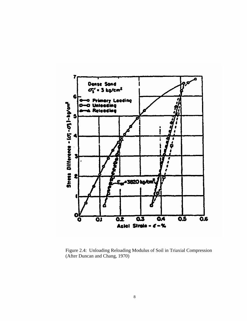
The deformation of sand in the unloading-reloading range that takes place at moderate stress levels (i.e., not close to the failure stress) can be approximately characterized as linear elastic (Holubec, 1968; Duncan and Chang, 1970; Coon and Evans, 1971; Lade and Duncan, 1975). The average secant modulus of the unloading-reloading loop was defined as the unloading-reloading modulus (Eur) by Duncan and Chang (1970), as shown in Figure 2.4. The unloading-reloading modulus is proportional to the confining stress (Duncan and Chang, 1970). The unloading-reloading modulus depends upon the change of the deviator stress in an unloading-reloading cycle (Makhlouf and Stewart, 1965). The unloading-reloading modulus increases if the change of deviator stress is held constant but the magnitude of minimum deviator stress is increased. With a constant magnitude of the maximum stress, the unloading-reloading modulus decreases with decreasing minimum deviator stress in unloading-reloading cycles.

The deformations of granular soils in the primary loading are almost unaffected by the previous unloading-reloading cycles that occur at lower stress levels (Makhlouf and Stewart, 1965; Ko and Scott, 1967). Unlike those in the primary loading stress path, the deformation of sand under a reloading stress path is very much dependent on the stress histories it has experienced.

5

Figure 2.1: Possible Stress Paths in Triaxial Compression (After Lade and Duncan, 1976)

6

Figure 2.2: Stress Paths of Conventional Triaxial Compression (After Lade and Duncan, 1976)

7

Figure 2.3: Stress Strain Curve from Cyclic Triaxial Compression Tests (After Holubec, 1968)

8

Figure 2.4: Unloading Reloading Modulus of Soil in Triaxial Compression (After Duncan and Chang, 1970)

9

Yoshimi et al. (1975) used an adaptation of a quicksand tank to reproduce

uniform void ratios in large samples of sand using a controlled upward flow of water. By reversing the direction of water flow, one-dimensional loading was induced over the entire sample. They found that a normally consolidated sand sample was about six times more compressible than a prestressed sample, even though their initial void ratios or densities were equal.

Lambrechts and Leonards (1978) conducted a series of triaxial compression tests under different stress paths to examine effects of stress history on deformation of sand. Each set of stress paths used in simulating different stress histories was a combination of stress-path segments including proportional loading, unloading, and reloading. At the end of each set of such stress paths, the axial stress was increased while maintaining a constant confining pressure as in a conventional triaxial test. They found that by prestressing the sand under Ko-condition, the modulus of deformation under the conventional triaxial compression loading increased by one order of magnitude.

Bishop and Eldin (1953) studied the effect of stress history on the angle of internal friction of sand by conducting a number of triaxial compression tests. They concluded that the angle of internal friction of sand is independent of the stress history. This conclusion was confirmed by Lade and Duncan (1976) and Lambrechts and Leonards (1978).

Based on the literature review outlined above, the behavior of sand subject to preloading-reloading loads is summarized as follows:

1. Elastic behavior can be assumed for sand under unloading-reloading cycles that take place at moderate stress levels.

2. A hysteresis loop exists in unloading-reloading cycles. The hysteresis loop indicates inelastic behavior and energy dissipation during unloading and reloading. The width or area of the hysteresis loop becomes significant during unloading and reloading at high stress levels.

3. An average secant modulus of the unloading-reloading loop can be represented by the unloading-reloading modulus (Eur). The unloading-reloading modulus (Eur) is proportional to the confining stress and also depends on maximum and minimum values of deviator stress change in the unloading-reloading cycles.

4. Deformation of sand under a reloading stress path is strongly influenced by the stress history. The deformation moduli increase significantly after the sand has been prestressed.

5. The angle of internal friction or the shear strength of sand is independent of the stress history.

10

2.2 Behavior of Geosynthetics Subject to Unloading-Reloading Cycles Some studies have been conducted by in-isolation cyclic load extension tests

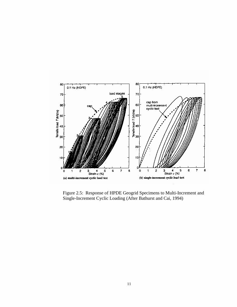
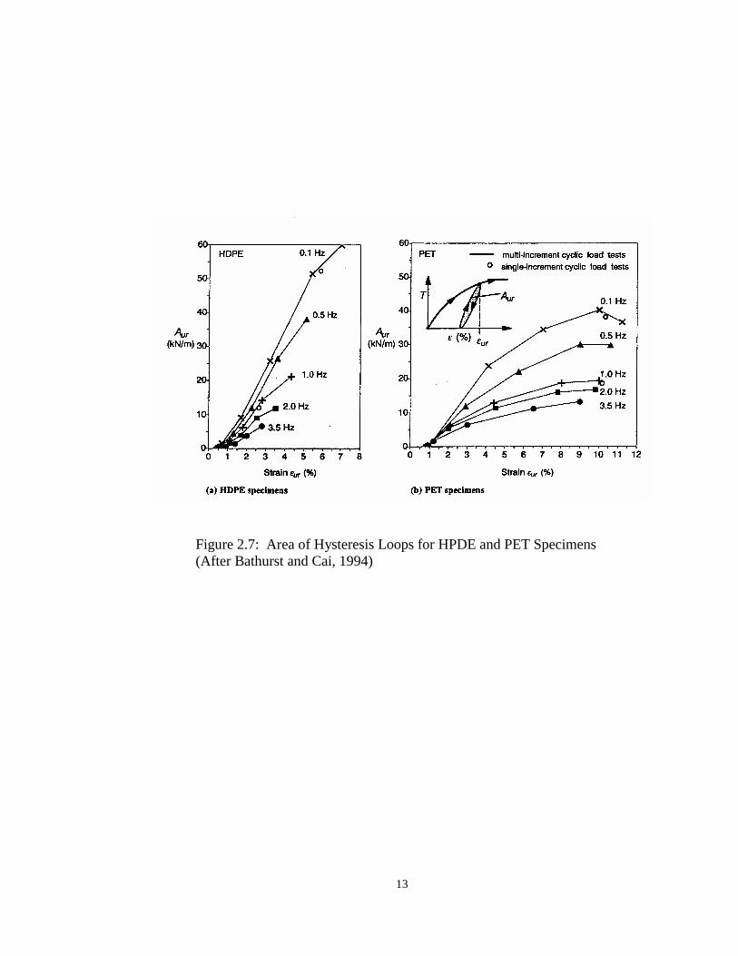
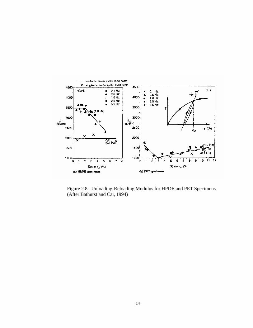
to examine the cyclic behavior of geosynthetics. Barthurst and Cai (1994) conducted a series of in-isolation cyclic load-extension tests on HDPE (high density polyethylene) and PET (polyester) geogrid specimens. The specimens were tested at different loading frequencies from 0.1 to 3.5 Hz and over a range of load amplitudes. Figure 2.5 shows typical load-strain response curves of the HPDE geogrid specimens under multi-increment and single-increment cyclic loadings. A hysteresis loop exists at all unloading-reloading cycles. Accumulative plastic strains due to multiple cycles of cyclic loading are evident. Some qualitative features of a cyclic load-deformation response curve are illustrated in Figure 2.6. Figure 2.6 identifies the parameters that can be used to characterize the load-deformation response as a function of strain. A non-linear hysteresis load-deformation loop for each unloading-reloading cycle (εur, Tur) is defined by the average unloading-reloading modulus (Jur) of the unloading-reloading cycle and its contained area (Aur). The area of a hysteresis loop (Aur) of the cyclic load-deformation curves of the geogrid specimens was found to be strongly influenced by the strain level and the frequency of loading. The area, Aur , increases with the strain level and decreases with increasing frequency at a given strain, as shown in Figure 2.7. It should be noted that below 0.5% strain of the HDPE geogrid and 0.8% strain of the PET geogrid, the specimens behaved in a linear elastic manner with fully recoverable strain. Figure 2.8 shows the average unloading-reloading modulus versus strain relationships for different load amplitudes and frequencies. The average unloading-reloading modulus, Jur, of the HDPE specimens reduces with the strain level, whereas the PET specimens showed a reduction of Jur up to about 3% of strains followed by an increase. Similar in-isolation cyclic load-extension tests on HDPE geogrids were conducted by Nocola and Montanelli (1997). The specimens were tested at different loading frequencies from 0.1 to 1.0 Hz and over different cyclic loading ranges. The tests showed that the unloading-reloading modulus, Jur, increases with strains until it reaches a yield point after which the unload-reload tensile modulus gradually decreases with increasing strains. In summary, the unloading-reloading behavior of geosynthetics can be quantified by the unloading-reloading modulus (Jur) and the area of a hysteresis loop (Aur). The hysteresis loop occurs when geosynthetics are subjected to unloading-reloading cycles. The area of hysteresis loop increases with strain level. At small strains (0.5% to 0.8%), the area of hysteresis loop becomes negligible, and the geogrids behave in a linear manner. For HPDE geogrids, the unloading-reloading modulus increases slightly with increasing strains until it reaches a “yield” point, after which the unloading-reloading modulus reduces with increasing strains.

11

Figure 2.5: Response of HPDE Geogrid Specimens to Multi-Increment and Single-Increment Cyclic Loading (After Bathurst and Cai, 1994)

12

Figure 2.6: Characteristics of Cyclic Response of Geosynthetic Specimen (After Bathurst and Cai, 1994)

13

Figure 2.7: Area of Hysteresis Loops for HPDE and PET Specimens (After Bathurst and Cai, 1994)

14

Figure 2.8: Unloading-Reloading Modulus for HPDE and PET Specimens (After Bathurst and Cai, 1994)

15

2.3 Behavior of Soil-Geosynthetic Interfaces Subject to Unloading-Reloading Cycles A limited number of works on the behavior the soil-geosynthetic interfaces subject to unloading-reloading cycles were available in the literature. O’Rourke et al. (1990) conducted a series of direct shear tests on Ottawa sand and HDPE geosynthetic. The tests showed that the shear strength of the interface was not affected by the repeated loading, as shown in Figure 2.9. Figure 2.10 shows the shear strength of the interface plotted versus number of repeated loadings before shear to failure. 2.4 Behavior of GRS Masses Subject to Unloading-Reloading Cycles 2.4.1 General Behavior A GRS mass is a soil mass embedded with layers of geosynthetic reinforcement. In this study, unless otherwise specified, the reinforcement layers are horizontally oriented. This section begins with a presentation of the strength and deformation behavior of a GRS mass, followed by the effects of preloading on a GRS mass.

Under vertical loading, a GRS mass shows a higher load carrying capacity than a soil mass without reinforcement. This reinforcing effect of reinforcement has been explained by an increased confinement concept by Yang (1974). The concept is illustrated by the Mohr stress diagram shown in Figure 2.10. The vertical and lateral stresses are assumed to be major and minor principal stresses, respectively. Circle A represents an at-failure stress state of a soil mass without reinforcement. The vertical and lateral stresses at failure for the soil mass are σ1 and σ3c, respectively (see Figure 2.10). With a reinforcement, the lateral stress at failure is increased by ∆σ3R, which is equal to the tensile strength of the reinforcement. As a consequence, the vertical stress at failure increases to σ1R, i.e., a higher load carrying capacity is obtained. It is assumed that there is no slippage at the soil-reinforcement interface and that failure of the reinforced soil mass is due to rupture of the reinforcement.

Under a vertical load, the GRS mass exhibits both lateral and vertical deformation responses. The soil expands laterally with the geosynthetic and mobilizes tensile forces in the geosynthetic through the friction between the soil and the geosynthetic. The tensile force in the geosynthetic restrains the lateral movement of the soil and, consequently, reduces the vertical deformation.

The effect of reinforcement in reducing deformation of a soil mass can be illustrated by triaxial compression test results conducted on unreinforced and reinforced soil samples by Gray and Al-Refeai (1987) as shown in Figure 2.11. Figure 2.11 shows that the stiffness or tangent moduli of the unreinforced and reinforced specimens are almost the same until 1.5% of axial strain. In other words, the internal restraining effect by the geosynthetic reinforcement is insignificant at

16

small strains. This is because the geosynthetic reinforcement requires some deformation in order to mobilize sufficient tensile force in the reinforcement.

Figure 2.11 also shows that at small strains (0 to 1.5%), the stiffness of a reinforced soil is somewhat smaller than that in the unreinforced soil. Similar behavior has been reported in triaxial compression tests by Broms (1977). Wu (1989) has investigated this effect and concluded that the loss of compressive stiffness in the reinforced soil is due to compression of the reinforcement itself. The effect of compressibility of the reinforcement is pronounced in the triaxial tests because ratios of the reinforcement spacing to the reinforcement thickness in the triaxial tests are relatively small. The loss of stiffness at the small strains because of the compressibility of the reinforcement is negligible in field construction because ratios of the reinforcement spacing to the reinforcement thickness are much greater than those in the triaxial tests.

Deformation of a GRS mass is of major concern when it is to be used in critical structures such as bridge piers and abutments. To limit the deformation of a GRS mass, a preloading concept is applied to increase the stiffness of the GRS structure (Tatsuoka et al., 1997). The preloading technique on a GRS mass takes advantage of the fact that soil stiffness is increased after it has been preloaded or prestressed. The preloaded GRS mass is also expected to behave nearly elastically in a reloading path similar to what has been observed in a preloaded soil.

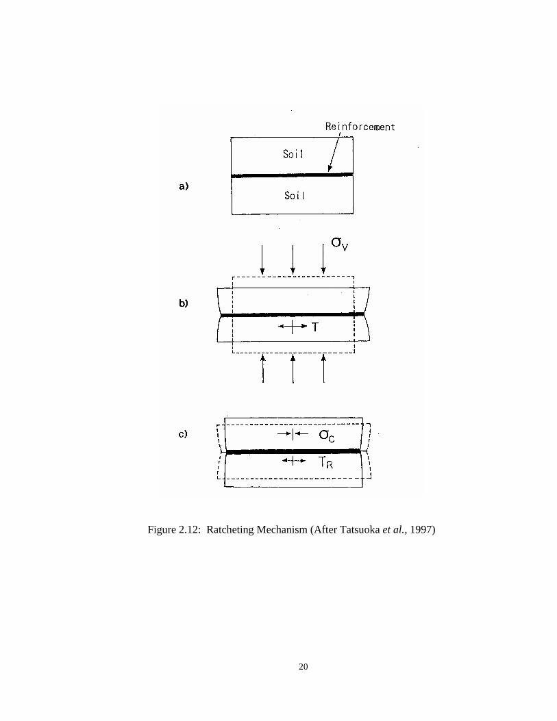
Preloading also mobilizes tensile strains in the geosynthetic reinforcement in a service condition--the so-called ratcheting mechanism (Tatsuoka et al., 1997). A simple model of a soil-geosynthetic composite shown in Figure 2.12 illustrates this mechanism. Under an applied pressure, σv, lateral deformation of the composite occurs and results in a tensile force in the reinforcement. Upon unloading, most of the lateral deformation of the soil does not rebound back. As a result, the reinforcement has been stretched and the tensile strains are mobilized. This mechanism also helps eliminating wrinkles that often occur during field placement of geosynthetic layers.

17

Figure 2.9: Interface Friction Angle as a Function of Number of Repeated Loadings for Ottawa Sand on HPDE (After O’Rourke et al., 1990)

18

Figure 2.10: Increased Confinement Concept of Soil Reinforcement (After Yang, 1974)

19

Figure 2.11: Stress-Strain Relationships from Triaxial Compression Tests on Reinforced Sand (After Gray and Al-Refeai, 1987)

20

Figure 2.12: Ratcheting Mechanism (After Tatsuoka et al., 1997)

21

2.4.2 Preloaded GRS Structures Since 1977, the preloading concept has been applied on the following four GRS structure:

1. Preloaded/Prestressed GRS walls in University of Tokyo, Tokyo, Japan (Tatsuoka et al., 1997);

2. Preloaded GRS pier in Turner-Fairbank Highway Research Center, McLean, Virginia, USA (Adams, 1997), referred to as the FHWA pier;

3. Preloaded/Prestressed GRS bridge pier in Fukuoka City, Japan (Uchimura et al., 1998);

4. Preloaded GRS bridge abutments in Black Hawk, Colorado, USA (Wu et al., 1999), referred to as the Black Hawk abutments.

2.4.2.1 Preloaded/Prestressed GRS Walls

Tatsuoka et al. (1997) proposed a new construction protocol, so-called preloaded/prestressed (PL/PS) reinforced soil. The main purpose was to make deformation of a GRS mass be nearly elastic and have a very high stiffness under applied loads.

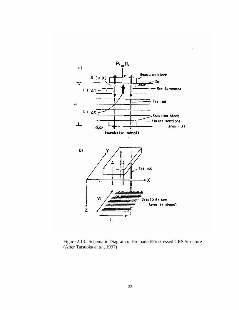
A schematic diagram of a PL/PS GRS structure is shown in Figure 2.13. Large preloading is applied by introducing tension into metallic tie rods that are intruded through the reinforced soil mass and fixed to the bottom reaction block. The tensile force in the tie rods and the corresponding compressive load in the backfill soil function as prestressing to maintain the vertical confining pressure and results in high stiffness in the vertical direction.

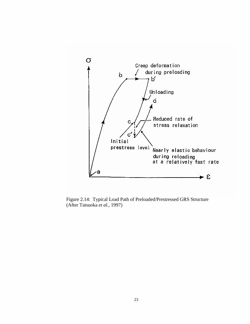
A typical PL/PS loading path involves preloading, sustained loading, unloading to a desired prestress loading level, and reloading as shown in Figure 2.14. A vertical load is applied up to a stress level, b, and sustained for a period of time. After allowing the creep deformation during the preloading stage to occur (b to b´), the load is reduced from b´ to c as unloading. The stress level, c, is defined as an initial prestress level. The vertical deformation is maintained constant at the stress level, c, and, consequently, the prestress level decreases from c to c´ due to plastic deformation of the GRS mass, known as the stress relaxation. A reloading stress path takes place from the stress level c´ to d. Full-scale loading tests of 5.4-m-high geogrid-reinforced walls were conducted at the University of Tokyo, Japan, to validate the PL/PS concept (Tatsuoka et al., 1997). The full-scale test results showed that the stiffness of the soil mass with compressive prestress was higher than that of the soil mass without prestress. Deformation of soil after preloading was nearly elastic for a relatively small load increment (Tatsuoka et al., 1997).

22

Figure 2.13: Schematic Diagram of Preloaded/Prestressed GRS Structure

(After Tatsuoka et al., 1997)

23

Figure 2.14: Typical Load Path of Preloaded/Prestressed GRS Structure (After Tatsuoka et al., 1997)

24

2.4.2.2 FHWA Pier A detailed description of the FHWA pier has been presented by Adams

(1997). A brief description of the project is given below. The GRS pier was 5.4 m high with base and top dimensions of 3.6 m x 4.8 m and 3.06 m x 4.26 m, respectively. The pier was constructed with a well-graded gravel (GW-GM per ASTM D2487) and reinforced with layers of geotextile sheets. The maximum dry density of the backfill was 24 kN/m3, and the optimum moisture content was 5.0%, per AASHTO T180. The average backfill density from nuclear density tests was 22.8 kN/m3. The reinforcement was a high-strength woven polypropylene geotextile, Amoco 2044. The vertical spacing of reinforcement was 0.2 m. Split face concrete (cinder) blocks, with dimensions of 0.2 m x 0.2 m x 0.4 m, were dry-stacked to form the facing. The front edge of each reinforcement sheet was placed between vertically aligned blocks to achieve a frictional connection between the reinforcement layer and the facing blocks. A schematic diagram of the pier is shown in Figure 2.15. The loading mechanism of the GRS pier comprised hydraulic jacks and a specially designed reaction system, as shown in Figure 2.16. The reinforced soil mass was sandwiched between the top and bottom concrete pads, which were connected together with vertical steel rods. The hydraulic jacks were placed between the top concrete pads and the reaction frame. Upon applying pressure to the hydraulic jacks, the GRS pier was “squeezed” between the top and bottom pads.

25

Figure 2.15: Principal Elements of FHWA Pier (After Adams, 1997)

26

Figure 2.16: Preloading Assembly of FHWA Pier (After Adams, 1997)

27

2.4.2.3 Preloaded/Prestressed GRS Walls A prototype 2.7 m-high PL/PS geogrid-reinforced soil bridge pier, as shown

in Figure 2.17, was constructed at Fukuoka City, Japan, to support temporary railway girders. It has been opened to service since the summer of 1997. Behavior of the prototype PL/PS bridge pier during and after construction and in service was reported by Uchimura et al. (1998). The prototype pier showed very small transient and long-term deformations compared with a nearby geogrid-reinforced bridge abutment constructed without preloading/prestressing subject to the same transient load from a locomotive (Uchimura et al.,1998).

2.4.2.4 Black Hawk Abutments

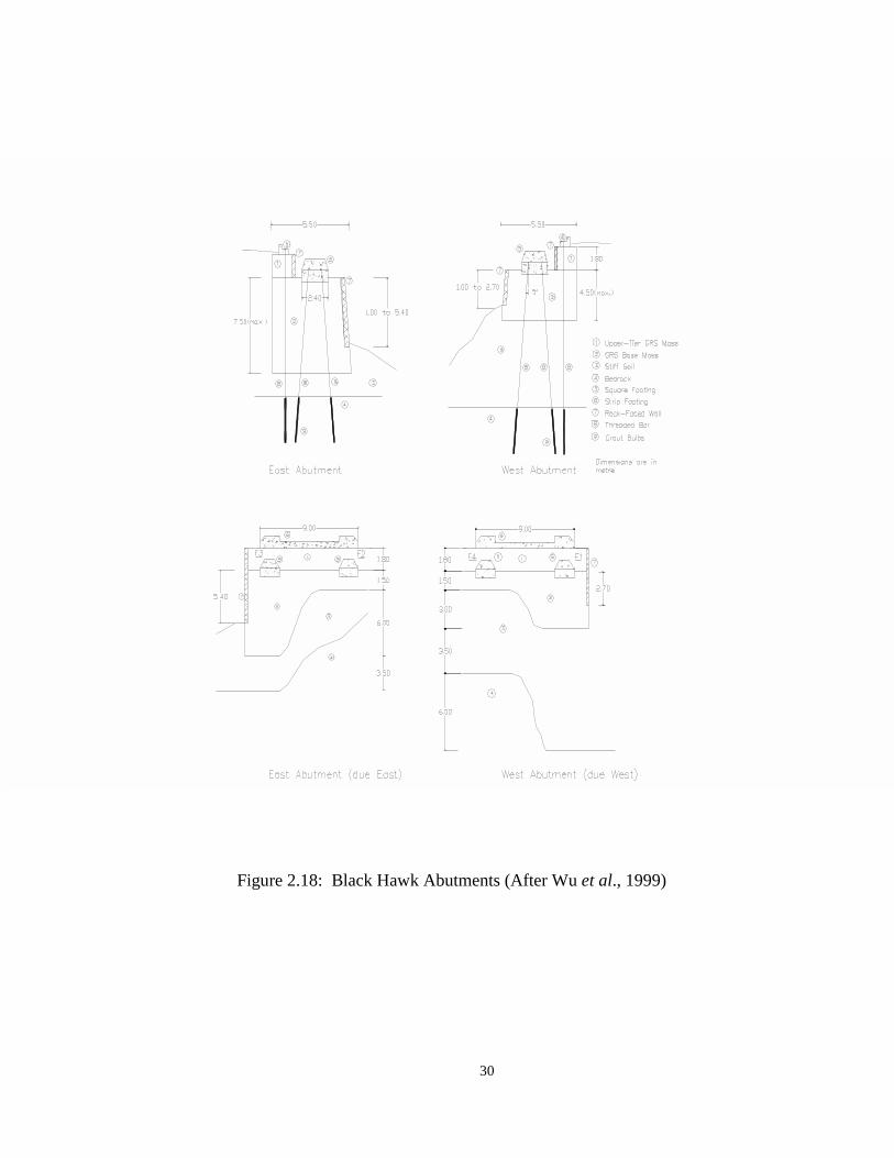
A detailed description of the Black Hawk abutments has been presented by Wu et al. (1999). A brief description of the project is given below. The abutments were constructed in the mountain terrain above the city of Black Hawk, Colorado, to support a 36-m span steel arched bridge. The abutments were constructed with the on-site soil (the Road Base soil used in the SGP test in this study) and reinforced with layers of a woven geotextile (Amoco 2044) having a vertical spacing of 0.3 m. Material properties of the soil and the reinforcement are presented in Chapter 3. The facing was of rock-faced type. The wall face was built by tightly stacking the rocks in rows about 0.3 m in height. The front edge of each reinforcement sheet was placed between vertically aligned rocks at the wall face to form a frictional connection between the reinforcement layers and the facing rocks. A series of sketches illustrating the geometry of the GRS abutments is shown in Figure 2.18. Each GRS abutment comprised a two-tier rock-faced GRS mass, two square footings (on the GRS base mass), and a strip footing (on the upper-tier GRS mass). Each abutment was constructed into a mountain slope on opposite sides of a stream valley with a silty stream deposit. The thickness of the silty soil layer was variable and considerably greater on the down slope side of the mountain. The slopes were excavated to remove the silty soil, which was considered unsuitable to support the abutments. The GRS abutments were supported on a stiff soil layer underneath the silty soil layer. As viewed from the faces (due east and west) (see Figure 2.18), the base of the GRS mass was located at different depths of the excavated stiff soil. The variable thickness of the GRS base mass was between 1.5 m and 7.5 m for the east abutment and 1.5 m and 4.5 m for the west abutment. The width at the base of the GRS base mass was 5.5 m. The lower part of the GRS base mass was embedded in the ground, and the upper part was above the ground. Only the portion above ground was constructed with rock facing. The height of the rock-faced wall varied from 1.0 m to 5.4 m in the east abutment and 1.0 m to 2.7 m in the west abutment. The upper-tier GRS mass was perched on the backside of each GRS base mass. The upper-tier GRS mass was 1.8 m thick and constructed in the same fashion as the GRS base mass.

28

The four square footings had a base area of 2.4 m x 2.4 m. The footing thickness was about 1.65 m. The final thickness depended on the amount of settlement due to preloading. The square footings on the west abutment were referred to as Footing #1 (F1) and #4 (F4). The square footings on the east abutment were referred to as Footing #2 (F2) and #3 (F3). The design load for each square footing was 865 kN, equivalent to a vertical pressure of 150 kPa. As shown in Figure 2.19, the preloading assembly for each footing consisted of four 534-kN hollow-cored jacks ganged together with a manifold and connected to a hydraulic electric pump. Each jack was placed on top of the square footing and connected to a threaded rod by inserting the rod through the core of the jack. The jack was sandwiched between the square footing and the steel bearing plates capped with a nut threaded on the rod. On two jacks, 890-kN load cells were inserted between the steel bearing plate and the nut. Installation of the threaded rods occurred after construction of the GRS base mass. A survey located the perimeter of the square footings and four prescribed points within the perimeter of the footing. At the points, a reticulating air-percussion rotary drill rig bored 90-mm diameter holes through the GRS mass, the stiff soil layer, and into the underlying bedrock. The bond length was about 3.5 m within the bedrock. To preload the GRS mass and the stiff soil layer underneath the footings, hydraulic oil was pumped into the hydraulic jacks. As the cylinders advanced, the GRS and the stiff soil were preloaded or “squeezed” between the footing and the bedrock. After the preloading, each borehole was sealed with a grout mix.

29

Figure 2.17: Prototype Preloaded/Prestressed GRS Bridge Pier (After Uchimura et al., 1998)

30

Figure 2.18: Black Hawk Abutments (After Wu et al., 1999)

31

Figure 2.19: Preloading Assembly of Black Hawk Abutments

32

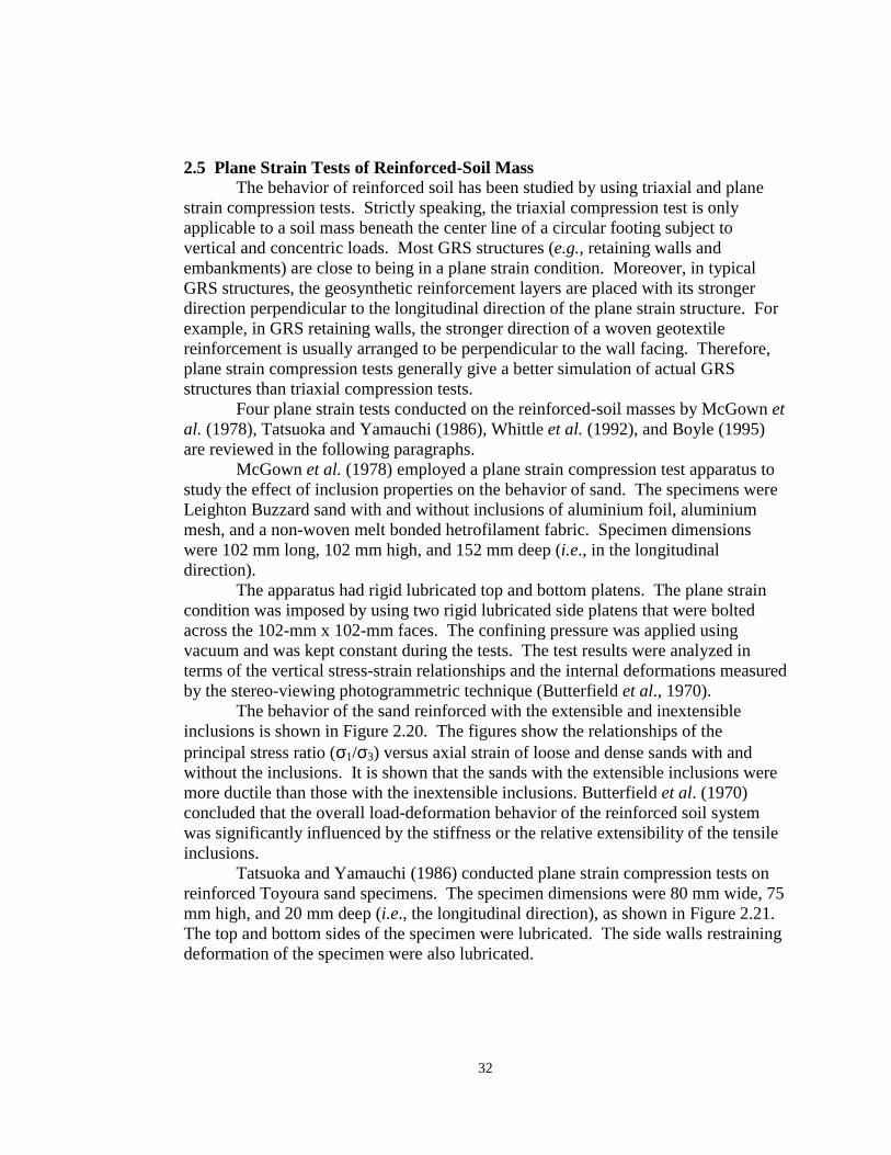
2.5 Plane Strain Tests of Reinforced-Soil Mass The behavior of reinforced soil has been studied by using triaxial and plane strain compression tests. Strictly speaking, the triaxial compression test is only applicable to a soil mass beneath the center line of a circular footing subject to vertical and concentric loads. Most GRS structures (e.g., retaining walls and embankments) are close to being in a plane strain condition. Moreover, in typical GRS structures, the geosynthetic reinforcement layers are placed with its stronger direction perpendicular to the longitudinal direction of the plane strain structure. For example, in GRS retaining walls, the stronger direction of a woven geotextile reinforcement is usually arranged to be perpendicular to the wall facing. Therefore, plane strain compression tests generally give a better simulation of actual GRS structures than triaxial compression tests. Four plane strain tests conducted on the reinforced-soil masses by McGown et al. (1978), Tatsuoka and Yamauchi (1986), Whittle et al. (1992), and Boyle (1995) are reviewed in the following paragraphs. McGown et al. (1978) employed a plane strain compression test apparatus to study the effect of inclusion properties on the behavior of sand. The specimens were Leighton Buzzard sand with and without inclusions of aluminium foil, aluminium mesh, and a non-woven melt bonded hetrofilament fabric. Specimen dimensions were 102 mm long, 102 mm high, and 152 mm deep (i.e., in the longitudinal direction). The apparatus had rigid lubricated top and bottom platens. The plane strain condition was imposed by using two rigid lubricated side platens that were bolted across the 102-mm x 102-mm faces. The confining pressure was applied using vacuum and was kept constant during the tests. The test results were analyzed in terms of the vertical stress-strain relationships and the internal deformations measured by the stereo-viewing photogrammetric technique (Butterfield et al., 1970).

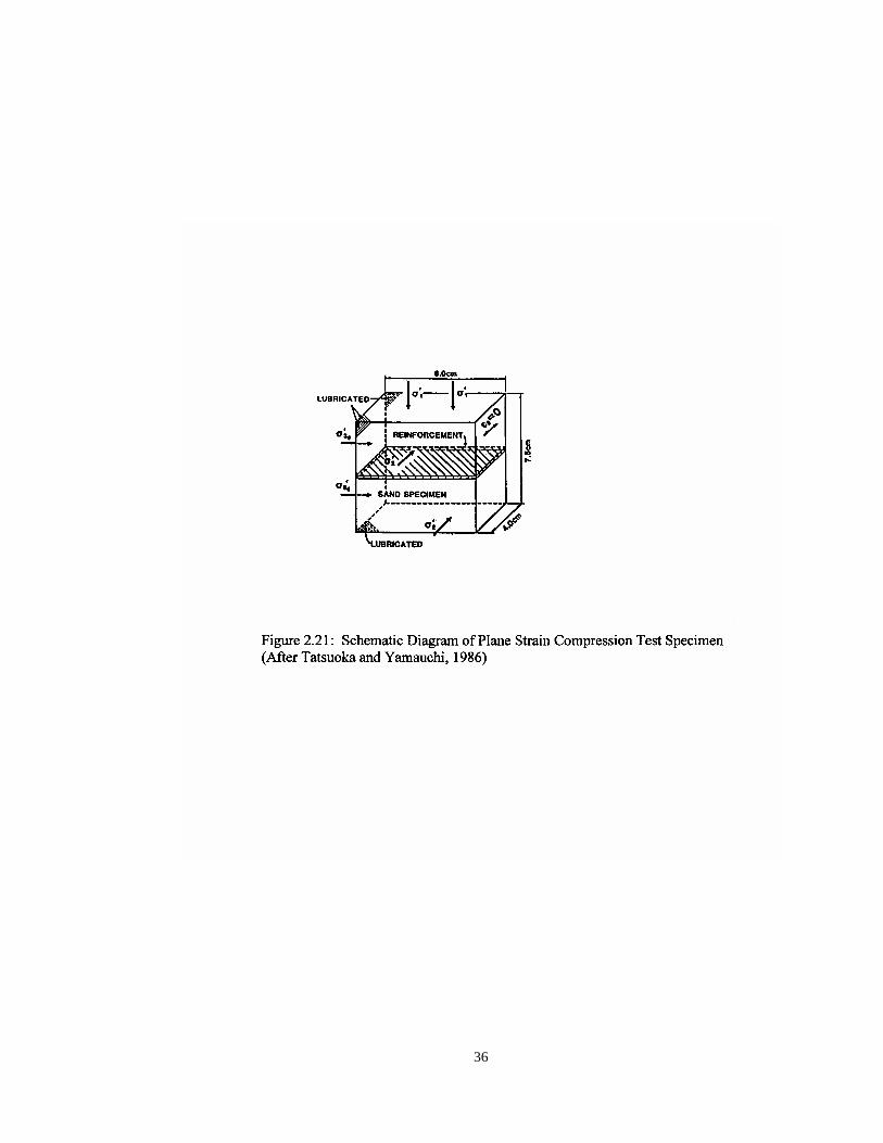
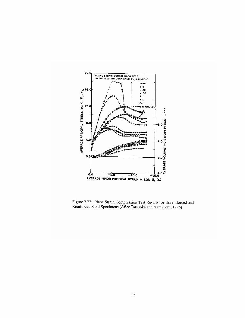
The behavior of the sand reinforced with the extensible and inextensible inclusions is shown in Figure 2.20. The figures show the relationships of the principal stress ratio (σ1/σ3) versus axial strain of loose and dense sands with and without the inclusions. It is shown that the sands with the extensible inclusions were more ductile than those with the inextensible inclusions. Butterfield et al. (1970) concluded that the overall load-deformation behavior of the reinforced soil system was significantly influenced by the stiffness or the relative extensibility of the tensile inclusions. Tatsuoka and Yamauchi (1986) conducted plane strain compression tests on reinforced Toyoura sand specimens. The specimen dimensions were 80 mm wide, 75 mm high, and 20 mm deep (i.e., the longitudinal direction), as shown in Figure 2.21. The top and bottom sides of the specimen were lubricated. The side walls restraining deformation of the specimen were also lubricated.

33

The reinforcement materials were brass plates, non-woven geotextiles, and different types of rubbers. The average principal stress difference (σ′1/σ′3) versus average minor principal strain (ε3) relationships of the soil are shown in Figure 2.22. The stress-strain relationships are similar to those of the plane strain tests conducted by McGown et al. (1978) (of Figure 2.20), in that the sand reinforced with stiff materials (brass plates) was more brittle than the sand reinforced with relatively less stiff materials (geotextiles and rubbers). The test results also indicated that, in order to mobilize a sufficient degree of tensile restraint in the composite, the non-woven geotextiles required a larger soil deformation in the reinforcement direction than the stiffer reinforcement materials. Whittle et al. (1992) devised an automated plane strain reinforcement (APSR) cell to study load transfer characteristics at working load levels of a reinforced-soil mass. Figure 2.23 shows a schematic diagram of the APSR cell. The soil specimen has dimensions of 570 mm high, 450 mm wide, and 150 mm deep (i.e., the longitudinal direction). The major principal stress (σ1< 500 kPa) was applied through two pressurized water bags mounted on moveable rigid platforms. A uniform lateral confinement (σ3< 50 kPa) was provided by air pressure. The maximum tensile stress in the reinforcement was measured at the end that was connected to a load cell. The stress in the reinforcement was induced by the stress developed in the confining soil resulting from the boundary stresses (σ1 and σ3 ). All contacted surfaces of the specimen to the apparatus were lubricated with silicone grease to minimize friction in the system. Whittle et al. (1992) reported the results of a test performed on a dry Ticino sand reinforced with two-ply steel sheet inclusions. A number of strain gauges were mounted between the two thin steel sheets (0.13 mm thick) to obtain the strain distribution within the reinforcement. The test results are shown in Figure 2.24. The figure shows the relationships of the load in the reinforcement versus the applied stress ratio (R=σ1/σ3). It was concluded that the tensile stress in the reinforcement was a linear function of the stress ratio, R. It also showed that the maximum tensile stress occurred at the center of the inclusion and that the tensile stresses in the reinforcement were minimal when the stress ratio, R, was less than 2. A plane strain unit cell device (UCD) was developed by Boyle (1995). The specimen dimensions were 200 mm high, 200 mm wide, and 100 mm deep (i.e., the longitudinal direction). Figure 2.25 shows schematic diagrams of the apparatus. The UCD was a load-controlled test apparatus. The vertical pressure was applied by the top and bottom air bladders to the surfaces of the specimen. The left instrument box was allowed to move freely in the horizontal direction. The lateral pressure was applied by the end bladder through the instrument box. The tensile forces at two ends of the reinforcement layer were measured by load cells. Stiff end plates that were linked to the clamps controlled that the soil and the reinforcement deform together in the horizontal direction. The vertical and the horizontal displacements, the major

34

principal stress, and the tension at two ends of the reinforcement layer were measured directly.

Two different sands, four woven geotextiles, two nonwoven geotextiles, and a steel sheet were employed in the study. Boyle (1995) reported similar results as those of the previous studies that the reinforcement improved the load carrying capacity of the dense cohesionless soil, as shown in Figure 2.26. The figure shows the relationships of the principal stress (σ1) versus lateral strain (ε3). The load carrying capacity of the soil specimen reinforced with geotextiles (reinforcing No.1 to 6) increased with the stiffness of the reinforcement that was presented in terms of the modulus at 5% strain. The sand reinforced with a steel sheet (No.7) showed significantly higher deformation modulus than those with the geotextile reinforcement before yielding occurred at about 0.3% of lateral strain.

A comparison of the specimen size, soil type, reinforcement types, and instrumentation of the four plane strain compression tests of reinforced-soil masses reviewed in this section is presented in Table 2.1. A shortcoming of these triaxial and plane strain compression tests performed on the GRS mass is their reduced dimensions. The relatively small dimensions of the test specimens prohibit testing of a representative reinforced-soil specimen of a typical GRS structure.

35

Figure 2.20: Behavior of a Unit Cell With and Without Inclusions: (a) Dense Sand and (b) Loose Sand (After McGown et al., 1978)

36

37

38

39

Figure 2.24: Stress Distribution in a Steel Inclusion of the APSR Cell (After Whittle et al., 1992)

40

41

42

43

3. Laboratory Tests on Soils, Geosynthetics, and Soil-Geosynthetic Interfaces Laboratory tests were conducted to examine the behavior of a number of soils,

geosynthetics, and soil-geosynthetic interfaces subject to monotonic loading and unloading-reloading cycle(s). The laboratory tests consisted of conventional triaxial compression (CTC) tests for soils, in- isolation load-extension (LE) tests for geosynthetics, and direct shear (DS) tests for soil-geosynthetic interfaces. Each test category employed two types of loading sequences: monotonic loading and unloading-reloading cycle(s). The monotonic- loading tests were conducted to examine the behavior of the materials and the interfaces subject to monotonic loading and to provide reference properties for assessing effects of preloading on the deformation and strength behavior. The unloading-reloading tests were conducted to examine the behavior subject to unloading-reloading cycle(s) and to assess effects of preloading on the deformation and strength behavior. Test specimens used for the monotonic- loading tests were referred to as virgin specimens, whereas test specimens used for the unloading-reloading tests were referred to as preloaded specimens.

This chapter presents test materials, test descriptions, specimen preparations, measurement, data reductions, test programs, test results, and discussions of test results of the laboratory tests.

3.1 Test Materials 3.1.1 Soils Two types of granular soils were used in this study: an Ottawa sand and a “Road Base” soil, designated as S and RB, respectively. The Ottawa sand was chosen because of its well-defined properties. The Road Base soil was a granular material that is commonly used as backfill for GRS retaining walls. It was selected in this study to examine the behavior of a generic preloaded GRS mass consisting of a typical construction backfill. The Ottawa sand used in this study was a subround uniform sand, with its gradation curve shown in Figure 3.1. The specific gravity of the sand is 2.65. The maximum and minimum unit weights, per ASTM D854, were 17.65 kN/m3 and 15.34 kN/m3, respectively. The Road Base soil used in this study was a dark brown, silty sand. It was a backfill material for the preloaded GRS abutments in Black Hawk, Colorado (Section 2.4.1.4). The soil was classified as SM-SC, per ASTM D2487. It has 12% of fine particles (passing #200 standard sieve). The gradation curve is shown in Figure 3.2. The plasticity index and the liquid limit were 6% and 27%, respectively. The maximum dry density was 18.75 kN/m3 with the optimum water content of 14.2%, per ASTM D698. The moisture content-dry unit weight relationship is shown in Figure 3.3.

44

Figure 3.1: Grain Size Distribution of Ottawa Sand

45

Figure 3.2: Grain Size Distribution of Road Base Soil

0

10

20

30

40

50

60

70

80

90

100

0.010.1110

Grain Diameter (mm)

Perc

ent P

assi

ng (%

)

46

Figure 3.3: Moisture Content-Dry Unit Weight Relationship of Road Base Soil

17

17.5

18

18.5

19

8 10 12 14 16 18 20

Moisture Content (%)

Dry

Uni

t Wei

ght (

kN/m

3 )

Max. Dry Unit Weight = 18.75 kN/m3

O.M.C. = 14.2 %

47

3.1.2 Geosynthetics Two types of geosynthetics, Amoco 2044 and Typar 3301, were used in this

study. Amoco 2044 represents a strong reinforcement material, whereas Typar 3301 represents a weak reinforcement material.

Amoco 2044 is a woven polypropylene geotextile. The wide-width tensile strengths, as provided by the manufacturer, in both fill and warp directions are 70 kN/m. Amoco 2044 was a reinforcement material used in the FHWA pier (Section 2.4.1.2) and the Black Hawk abutments (Section 2.4.1.4). Some index properties of Amoco 2044 are shown in Table 3.1. Typar 3301 is a non-woven heat-bonded polypropylene geotextile. It was primarily used for filtration and drainage applications in actual applications. Some index properties of Typar 3301 are shown in Table 3.1.

48

Table 3.1: Some Index Properties of Geosynthetics

Geosynthetic Amoco 2044 Typar 3301

Manufacturing method Woven Non-Woven

Wide-width tensile strength 70 kN/m 6 kN/m (ASTM D-4595) (fill and warp directions)

Elongation at break 8% (fill direction) 70% (ASTM D-4595) 10% (warp direction)

Grab tensile 2.22 kN (fill direction) 0.53 kN

(ASTM D-4632) 2.67 kN (warp direction)

Elongation at break 20% 60% (ASTM D-4632) (fill and warp directions)

49

3.2 Loading System The loading system used in this study was the MTS-810 electro-hydraulic

testing system. The MTS-810 testing system comprised a loading frame integrated with a data acquisition system and a control unit. The loading frame (MTS Model 311.31) consisted of four vertical columns that joined a moveable crosshead and a fixed platen (see Figure 3.4). The crosshead was vertically adjustable to accommodate specimens of various heights. The vertical movement of the crosshead was controlled by hydraulic crosshead lifts. The crosshead, once in position, locked into place to prevent slippage during testing. The data acquisition system included a load cell with a maximum capacity of 1,000 kN (sensitivity = +0.04 kN) and LVDT (linear variable differential transformer) with a maximum displacement of 150 mm (sensitivity = +0.03 mm). The LVDT is an electromechanical device that provides an output voltage that is proportional to the displacement of a moveable core extension or a stylus. The LVDT was internally mounted on the hydraulic actuator to provide an indication of the actuator piston rod displacement. The MTS-810 loading system used the MTS458.20 MicroConsole as a control unit to control the servohydraulic system.

The data acquisition system and the control unit were connected to an IBM personal computer. A BASIC software for the control unit and the data acquisition system developed at the University of Colorado at Denver was modified by the author for this study. The modified BASIC software provided the inputs (stress-controlled or strain-controlled modes) for the control unit and recorded the outputs (load and displacement) from the data acquisition system. All input parameters must be predetermined and programmed in the IBM personal computer before starting a test. For the stress-controlled mode, the failure load of the specimen needs to be estimated beforehand to set an upper bound for the loading magnitude input. It is to be noted that the stress-controlled mode must never be used to load the specimen to failure. This is because a premature failure may damage the testing system.

3.3 Loading Sequences In this study, the monotonic loading was applied in a strain-controlled mode at a constant strain rate. The unloading-reloading cycles were applied in a stress-controlled mode at a constant loading rate. The unloading-reloading cycles were an array of different combinations of five loading paths: preloading (PL), unloading to a zero-load level (UL-Z), unloading to a prestressed load level (UL-PS), reloading from a zero-load level (RL-Z), and reloading from a prestressed load level (RL-PS). A diagram illustrating the applied load versus time relationships for 1) PL, UL-Z, and RL-Z paths, and 2) PL, UL-PS, and RL-PS paths are shown in Figure 3.5. In this report, the term “applied load” is used to represent different quantities for different types of tests. It represents the deviator stress in CTC tests, the applied tensile load in LE tests, the shear stress in DS tests, and the vertical load from the MTS-810 loading

50

device in SGP tests. The unloading load level (ULL) was equal to the zero-load level for the UL-Z and RL-Z paths, and the prestressed load level (PSL) for the UL-PS and RL-PS paths. The minimum unloading load level was the zero- load level. The zero-load level was considered the initial stress of the specimen; i.e., the applied load = 0.

As shown in Figure 3.5, the PL path begins at t = 0 and increases at a constant loading rate to a PLL. An unloading path (UL-Z or UL-PS path) follows the PL path. The UL-Z path involves a decrease of the loading magnitude from a preloading load level to a zero- load level (i.e., ULL = 0). The RL-Z path follows the UL-Z path. The UL-PS path involves a decrease of the loading magnitude from a preloading load level to a prestressed- load level (i.e., ULL = PSL). The RL-PS path follows the UL-PS path. The preloading path resumes when the magnitude of the load in the reloading path exceeds the preloading load level.

51

Figure 3.4: MTS-810 Loading System

52

Figure 3.5: General Loading Sequences

UL

ULL

PLL

Applied Load

PL

RL

Time

Two unloading-reloading paths

1) When ULL = 0 => UL-Z, and RL-Z paths 2) When ULL = PSL => UL-PS, and RL-PS paths

53

3.4 Conventional Triaxial Compression Tests for Soils A series of CTC tests under monotonic loading and unloading-reloading

cycles were conducted on the two soils described in Section 3.1.1. The purposes of the tests were to examine the behavior of the soils subject to unloading-reloading cycles and to calibrate soil model parameters in the finite element analysis and the SPR model (Sections 5.3 and 6.3).

3.4.1 Test Description

The CTC test was performed on an unsaturated soil specimen. The triaxial chamber was placed in the MTS loading device as shown in Figure 3.6. Confining pressure was applied to the specimen by pressurizing the water surrounding the specimen. The applied vertical load and the vertical displacement of the loading rod were recorded by a data acquisition system integrated with the MTS-810 loading device. The volume-change occurred during shear was measured by monitoring the volume change of water entering or leaving the triaxial chamber.

3.4.2 Specimen Preparation and Test Procedure

The Ottawa sand specimen in the triaxial tests was 158 mm high and 71 mm in diameter. The specimen was prepared at a unit weight of 16.85 kN/m3 (+0.15 kN/m3). The specimen preparation and the test procedure for the Ottawa sand are as follows:

1. Obtain the dry Ottawa sand from the batch. 2. Use o-rings to attach a 0.2-mm-thick rubber membrane to the base platen. 3. Place a porous stone at the base of the platen. 4. Place a metallic mold (a split-barrel type) around the rubber membrane and

fold the top portion of the membrane down and over the mold. 5. Pour the sand in the mold by using 50-mm-diameter funnel with the opening

diameter of 5 mm at a constant drop height of approximately 80 mm. 6. Place a porous stone on top of the specimen. 7. Place the top platen on the porous stone and roll the rubber membrane over

the top platen and seal to the circumference of the top platen with o-rings. 8. Apply a vacuum pressure of 35 kPa on the specimen through the back

pressure valve that is connected to the base of the specimen. 9. Remove the metallic mold and obtain the average height and average diameter

of the specimen by using a stand ruler and a π−tape. 10. Place a lucite cylinder on the cell base. 11. Place the triaxial chamber in an MTS-810 loading frame. 12. Apply a predetermined confining pressure and open the back pressure valve. 13. After 15 minutes of consolidation with the confining pressure, start to apply

shear stress at a prescribed strain or loading rate.

54

14. Record the vertical applied load, the axial displacement, and the volume change of the specimen during shear. The Road Base soil specimen in the CTC tests was 305 mm high and 152 mm

in diameter. The specimen was prepared at a dry unit weight of 17.81 kN/m3 (+0.1 kN/m3) with a water content of 12.2%. The specimen preparation and the test procedure for the Road Base soil are as follows:

1. Prepare the soil at the desired moisture content of 12.2% and cure overnight in a sealed container inside a high humidity room.

2. Use o-rings to attach a 0.3-mm-thick rubber membrane to the base platen. 3. Place a porous stone at the base of the platen. 4. Place a metallic mold (a split-barrel type) around the rubber membrane and

fold the top portion of the membrane down and over the mold. 5. Compact the soil inside the mold in 12 layers by a 4- lb standard Proctor

hammer at the prescribed density. 6. Place a porous stone on top of the specimen. 7. Place the top platen on the porous stone and roll the rubber membrane over

the top platen and seal to the circumference of the top platen with o-rings. 8. Apply a vacuum pressure of 35 kPa on the specimen through the back

pressure valve that is connected to the base of the specimen. 9. Remove the metallic mold and attach a second layer of rubber membrane to

the specimen with o-rings on the top and base platens. 10. Obtain the average height and average diameter of the specimen by using a

stand ruler and a π−tape. 11. Place a lucite cylinder on the cell base. 12. Fill the triaxial chamber with water. 13. Place the triaxial chamber in an MTS-810 loading frame. 14. Apply a predetermined confining pressure and open the back pressure valve. 15. After 1 hour of consolidation with the confining pressure, start to apply shear

stress at a prescribed strain or loading rate. 16. Record the vertical applied load, the axial displacement, and the volume

change of the specimen during shear.

55

Figure 3.6: Conventional Triaxial Compression Test Apparatus

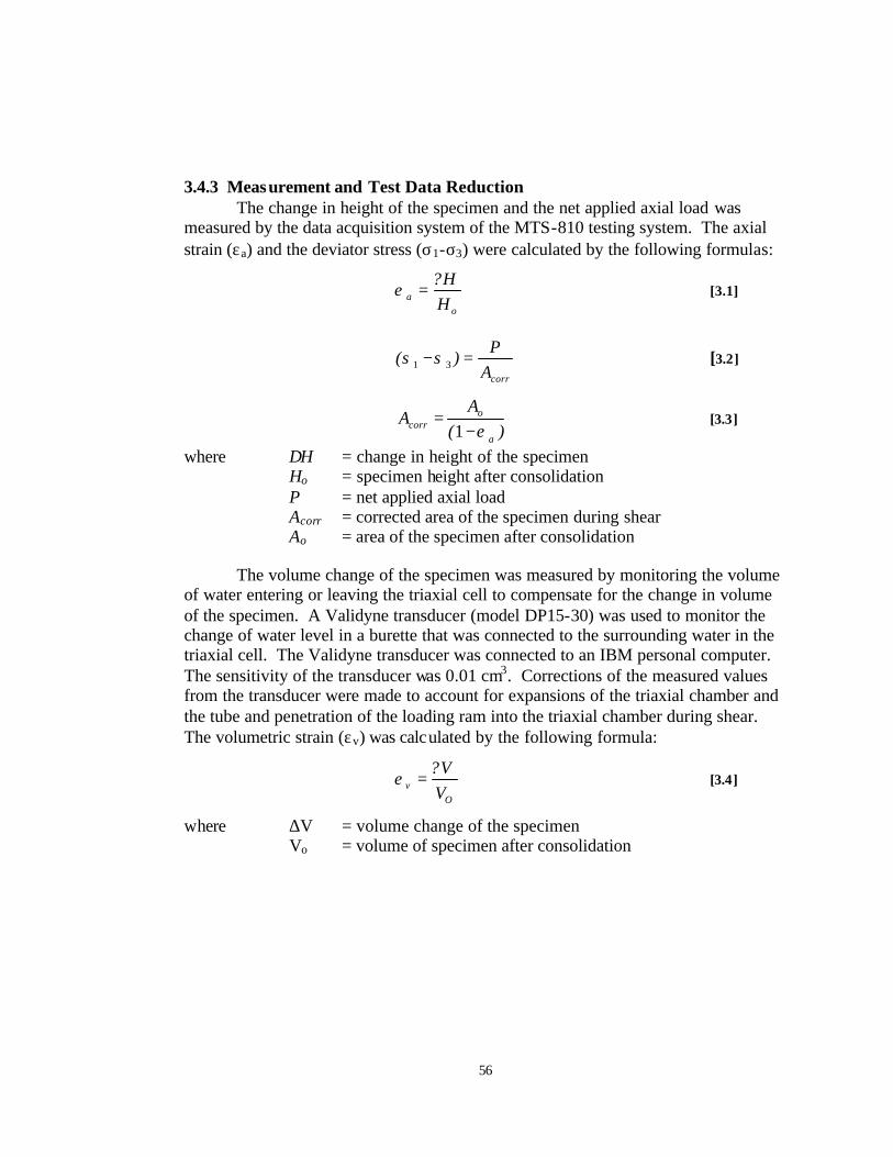
56

3.4.3 Measurement and Test Data Reduction

The change in height of the specimen and the net applied axial load was measured by the data acquisition system of the MTS-810 testing system. The axial strain (εa) and the deviator stress (σ1-σ3) were calculated by the following formulas:

oa H

?He = [3.1]

corrAP)s(s =− 31 [3.2]

)e(

AA

a

ocorr −

=1

[3.3]

where ∆Η = change in height of the specimen Ho = specimen height after consolidation P = net applied axial load Acorr = corrected area of the specimen during shear Ao = area of the specimen after consolidation

The volume change of the specimen was measured by monitoring the volume of water entering or leaving the triaxial cell to compensate for the change in volume of the specimen. A Validyne transducer (model DP15-30) was used to monitor the change of water level in a burette that was connected to the surrounding water in the triaxial cell. The Validyne transducer was connected to an IBM personal computer. The sensitivity of the transducer was 0.01 cm3. Corrections of the measured values from the transducer were made to account for expansions of the triaxial chamber and the tube and penetration of the loading ram into the triaxial chamber during shear. The volumetric strain (εv) was calculated by the following formula:

Ov V

?Ve = [3.4]

where ∆V = volume change of the specimen Vo = volume of specimen after consolidation

57

3.4.4 Test Programs Test programs for the CTC tests are presented in Table 3.2 for the Ottawa sand and Table 3.3 for the Road Base soil. The test program was divided into two groups: monotonic- loading (M) tests and unloading-reloading (UR) tests. Designations of all the tests are shown in the tables. The monotonic- loading tests were conducted in a strain-controlled mode at a constant strain rate of 0.5% per minute. The unloading-reloading tests were conducted in a stress-controlled mode with various loading sequences at a constant loading rate of 10 kPa per minute and followed by a strain-controlled mode at a constant strain rate of 0.5% per minute until failure occurred.

58

Table 3.2: CTC Test Program for the Ottawa Sand

59

Table 3.3: CTC Test Program for the Road Base Soil

60

3.4.5 Test Results and Discussions The CTC test results and discussions of the test results are presented in the following sections. The general behavior was first described, followed by an assessment of the effects of preloading on deformation and shear strength of the soils. 3.4.5.1 General Behavior The peak or maximum deviator stress generally corresponds to the failure state of the specimen. When the deviator stress continued to increase without showing a peak value, the deviator stress at 10% axial strain was considered the maximum deviator stress. A positive sign of the volumetric strain represents specimen dilation; whereas, a negative sign represents specimen contraction.

Figures 3.7 and 3.8 show the results of the monotonic-loading CTC tests. The deviator stress increased with the axial strain until failure occurred. The Ottawa sand initially contracted during shear and started to dilate at axial strains less than 0.8%. Similar to the sand, the Road Base soil at lower confining pressures contracted initially and dilated after it reached certain axial strains. The Road Base soil experienced dilatancy at larger axial strains (1.2% and 6% at confining pressures of 69 kPa and 207 kPa, respectively) than the Ottawa sand. At the confining pressure of 345 kPa, the Road Base soil specimen did not show the dilatant behavior.

Figures 3.9 to 3.14 show the results of the unloading-reloading CTC tests. The stress-strain curve was similar to the typical stress-strain curve of a soil specimen in the CTC test subject to primary loading, unloading, and reloading as described in Section 2.1.

The specimen was initially loaded to a preloading load level, then unloaded. Irrecoverable and recoverable deformations occurred when the specimen was unloaded. This behavior may be explained in terms of deformation of grains and sliding between grains (see, e.g., Makhlouf and Stewart, 1965; Ko and Scott, 1967; Lade and Duncan, 1976). The recoverable deformation was due to the elastic deformation of individual grains, whereas the irrecoverable deformation was primarily caused by the sliding between individual grains. In the primary loading, both the elastic deformation and sliding between grains occurred. Upon unloading, individual grains did not rebound to their original positions but remained approximately in their displaced positions. This behavior caused the irrecoverable deformation.

During the initial unloading path in which the deviator stress started to reduce, it was observed that axial and volumetric strains still continued to behave in the same fashion as those in the PL path. Specifically, the downward deformation continued and the volume change behavior was in expansion for the Ottawa sand and in contraction for the Road Base soil. This behavior has been reported in cyclic triaxial tests as a rounded corner of hysteresis loops (Hyodo et al., 1994) and explained in terms of creep of a soil specimen by Tatsuoka and Shibuya (1991). The magnitude of

61

the creep deformation was found to be more significant when the specimen was unloaded from a high preloading load level.

It is the author opinion that the influence of soil creep at an initial unloading path is suppressed in an unloading-reloading CTC test conducted in a strain-controlled mode. This is believed to be a strain-controlled loading characteristic. Under the strain-controlled mode, the vertical deformation of the specimen is controlled by vertical movements of the loading rod. It is tacitly assumed that the specimen is in full contact with the loading rod. The unloading path begins when the loading rod movement is reversed. This unloading mechanism eliminates the possibility of the soil to continue the vertical downward deformation during the unloading path.

When the specimen was unloaded and reloaded from small to moderate preloading load levels, it behaved approximately linear-elastically. However, when the unloading path took place at a high preloading load level (i.e., close to failure), the linearity between stress and strain may not be assumed as a result of significant hysteresis loops. The hysteresis loop existed in all unloading-reloading portions of deviator stress-axial strain curves. The width of the hysteresis loop is typically larger at the high preloading load level.

62

Figure 3.7: Test Results of Monotonic-Loading CTC Tests on Ottawa Sand (Tests T-M-S1, 2, and 3)

0

200

400

600

800

1000

1200

0 2 4 6 8 10 12

Axial Strain (%)

Dev

iato

r Str

ess

(kPa

)

345 kPa

207 kPa

69 kPa

-0.5

0.0

0.5

1.0

1.5

2.0

2.5

3.0

3.5

4.0

4.5

0 2 4 6 8 10 12

Axial Strain (%)

Volu

met

ric S

train

(%)

69 kPa

207 kPa

345 kPa

63

Figure 3.8: Test Results of Monotonic-Loading CTC Tests on Road Base Soil (Tests T-M-RB1, 2, and 3)

0

200

400

600

800

1000

0 2 4 6 8 10 12 14

Axial Strain (%)

Dev

iato

r Str

ess

(kPa

)

345 kPa

207 kPa

69 kPa

-4

-3

-2

-1

0

1

2

3

0 2 4 6 8 10 12 14

Axial Strain (%)

Volu

met

ric S

train

(%)

69 kPa

207 kPa

345 kPa

64

Figure 3.9: Results of Test T-UR-S1 (Confining Pressure = 69 kPa)

0

50

100

150

200

250

0 2 4 6 8 10 12

Axial Strain (%)

Dev

iato

r Stre

ss (k

Pa)

-0.5

0.0

0.5

1.0

1.5

2.0

2.5

3.0

3.5

4.0

0 2 4 6 8 10 12

Axial Strain (%)

Volu

met

ric S

train

(%)

65

Figure 3.10: Results of Test T-UR-S2 (Confining Pressure = 207 kPa)

0

100

200

300

400

500

600

0 2 4 6 8 10 12

Axial Strain (%)

Dev

iato

r Str

ess

(kPa

)

-0.5

0.0

0.5

1.0

1.5

2.0

2.5

3.0

3.5

4.0

0 2 4 6 8 10 12

Axial Strain (%)

Volu

met

ric S

trai

n (%

)

66

Figure 3.11: Results of Test T-UR-S3 (Confining Pressure = 345 kPa)

0

200

400

600

800

1000

1200

0 2 4 6 8 10 12

Axial Strain (%)

Dev

iato

r Str

ess

(kPa

)

-0.5

0.0

0.5

1.0

1.5

2.0

2.5

3.0

3.5

4.0

0 2 4 6 8 10 12

Axial Strain (%)

Volu

met

ric S

trai

n (%

)

67

Figure 3.12: Results of Test T-R-RB1 (Confining Pressure = 69 kPa)

0

50

100

150

200

250

300

0 2 4 6 8 10

Axial Strain (%)

Devi

ator

Stre

ss (k

Pa)

-0.60

-0.40

-0.20

0.00

0.20

0.40

0.60

0.80

1.00

0 2 4 6 8 10

Axial Strain (%)

Volu

met

ric S

trai

n (%

)

68

Figure 3.13: Results of Test T-UR-RB2 (Confining Pressure = 207 kPa)

0

100

200

300

400

500

600

0.0 2.0 4.0 6.0 8.0 10.0 12.0

Axial Strain (%)

Devi

ator

Stre

ss (k

Pa)

-3.00

-2.50

-2.00

-1.50

-1.00

-0.50

0.00

0.50

0.0 2.0 4.0 6.0 8.0 10.0 12.0

Axial Strain (%)

Volu

met

ric S

trai

n (%

)

69

Figure 3.14: Results of Test T-UR-RB3 (Confining Pressure = 345 kPa)

0

100

200

300

400

500

600

700

800

900

1000

0 2 4 6 8 10 12

Axial Strain (%)

Devi

ator

Stre

ss (k

Pa)

-3.00

-2.50

-2.00

-1.50

-1.00

-0.50

0.00

0.50

0.0 2.0 4.0 6.0 8.0 10.0 12.0

Axial Strain (%)

Volu

met

ric S

trai

n (%

)

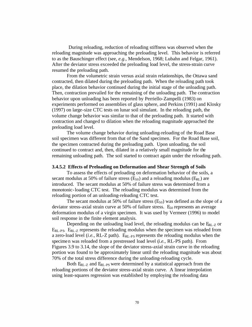
70

During reloading, reduction of reloading stiffness was observed when the reloading magnitude was approaching the preloading level. This behavior is referred to as the Bauschinger effect (see, e.g., Mendelson, 1968; Lubahn and Felgar, 1961). After the deviator stress exceeded the preloading load level, the stress-strain curve resumed the preloading path.

From the volumetric strain versus axial strain relationships, the Ottawa sand contracted, then dilated during the preloading path. When the reloading path took place, the dilation behavior continued during the initial stage of the unloading path. Then, contraction prevailed for the remaining of the unloading path. The contraction behavior upon unloading has been reported by Perriello-Zampelli (1983) on experiments performed on assemblies of glass sphere, and Perkins (1991) and Klosky (1997) on large-size CTC tests on lunar soil simulant. In the reloading path, the volume change behavior was similar to that of the preloading path. It started with contraction and changed to dilation when the reloading magnitude approached the preloading load level.

The volume change behavior during unloading-reloading of the Road Base soil specimen was different from that of the Sand specimen. For the Road Base soil, the specimen contracted during the preloading path. Upon unloading, the soil continued to contract and, then, dilated in a relatively small magnitude for the remaining unloading path. The soil started to contract again under the reloading path.

3.4.5.2 Effects of Preloading on Deformation and Shear Strength of Soils

To assess the effects of preloading on deformation behavior of the soils, a secant modulus at 50% of failure stress (E50) and a reloading modulus (ERL) are introduced. The secant modulus at 50% of failure stress was determined from a monotonic- loading CTC test. The reloading modulus was determined from the reloading portion of an unloading-reloading CTC test.

The secant modulus at 50% of failure stress (E50) was defined as the slope of a deviator stress-axial strain curve at 50% of failure stress. E50 represents an average deformation modulus of a virgin specimen. It was used by Vermeer (1996) to model soil response in the finite element analysis.

Depending on the unloading load level, the reloading modulus can be ERL-Z or ERL-PS. ERL-Z represents the reloading modulus when the specimen was reloaded from a zero-load level (i.e., RL-Z path). ERL-PS represents the reloading modulus when the specimen was reloaded from a prestressed load level (i.e., RL-PS path). From Figures 3.9 to 3.14, the slope of the deviator stress-axial strain curve in the reloading portion was found to be approximately linear until the reloading magnitude was about 70% of the total stress difference during the unloading-reloading cycle.

Both ERL-Z and ERL-PS were determined by a statistical approach from the reloading portions of the deviator stress-axial strain curve. A linear interpolation using least-squares regression was established by employing the reloading data

71

between 0% and 70% of the total stress difference during the unloading-reloading cycle. The slope of the linear interpolation was the reloading modulus.

Figures 3.15 and 3.18 show the relationships of reloading modulus (ERL-Z and

ERL-PS) versus f

PL

)−)−

31

31

((

σσσσ

of the Ottawa sand and the Road Base soil. The value of

f

PL

)−)−

31

31

((

σσσσ

is an indication of the preloading load level with respect to the failure

load. The average value of the reloading modulus at a given confining pressure was calculated and presented in the figures. It can be seen that the reloading modulus increased with increasing confining pressures. At the same confining pressure, the

reloading moduli tended to reduce with increasing f

PL

)−)−

31

31

((

σσσσ

. At f

PL

)−)−

31

31

((

σσσσ

=

0.8, the reloading modulus was about 0.85 to 0.95 of the average reloading modulus. ERL-Z and ERL-PS were compared with E50 to examine the effects of preloading

on deformation of the soils. Figures 3.19 and 3.20 show average deformation modulus versus confining pressure relationships of the Sand and the Road Base soil, respectively. As shown in Figures 3.19 and 3.20, E50 , ERL-Z , and ERL-PS increased with increasing confining pressures. At the same confining pressure, ERL-PS, ERL-Z, and E50 had the maximum, medium, and minimum values, respectively. The reloading modulus of the Ottawa sand was larger than E50 by factors of 1.5 to 3 for ERL-Z and 3 to 4 for ERL-PS. For the Road Base soil, the reloading modulus was larger than E50 by factors of 4.5 to 6.5 for ERL-Z and 6 to 9 for ERL-PS. These results indicate that 1) the preloaded specimen has much higher deformation modulus than the virgin specimen, and 2) the RL-SP path is more effective for increasing the deformation modulus than the RL-Z path. Effects of preloading on shear strength of the Ottawa sand and the Road Base soil were examined by a means of Mohr-Coulomb shear strength parameters (i.e., internal friction angle and cohesion). The shear strength parameters were determined from the p-q diagram at failure as shown in Figures 3.21 and 3.22. The friction angle of the Ottawa sand was 37.4° from the monotonic loading tests and 36.0° from the unloading-reloading tests. The friction angle and the cohesion of the Road Base soil were 31.4° and 32.9 kPa from the monotonic loading tests and 32.0° and 34.2 kPa from the unloading-reloading tests. These results indicate that the effects of preloading on the shear strength of the soils are insignificant. This finding is consistent with Bishop and Eldin (1953), Lade and Duncan (1976), and Lambrechts and Leonard (1978). This behavior may be explained by the relatively large deformation that occurred before and during failure. The displacements of the soil grains during failure are probably large enough to erase the preloading effects.

72

Figure 3.15: ERL-Z versus f

PL

)−)−

31

31

((

σσσσ

Relationships of Ottawa Sand

0

50

100

150

200

250

300

350

0.0 0.2 0.4 0.6 0.8 1.0

(σ 1 - σ 3 ) PL/(σ 1 - σ 3) f

ERL-

Z (M

Pa)

69 kPa207 kPa345 kPa

Avg. =326.4 MPa

Avg. =208.2 MPa

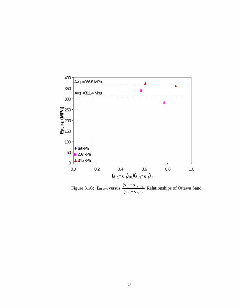
73

Figure 3.16: ERL-PS versus f

PL

)−)−

31

31

((

σσσσ

Relationships of Ottawa Sand

0

50

100

150

200

250

300

350

400

0.0 0.2 0.4 0.6 0.8 1.0(σ 1 - σ 3) PL/(σ 1 - σ 3) f

E RL-

PS (M

Pa)

69 kPa207 kPa345 kPa

Avg. =366.8 MPa

Avg. =311.4 Mpa

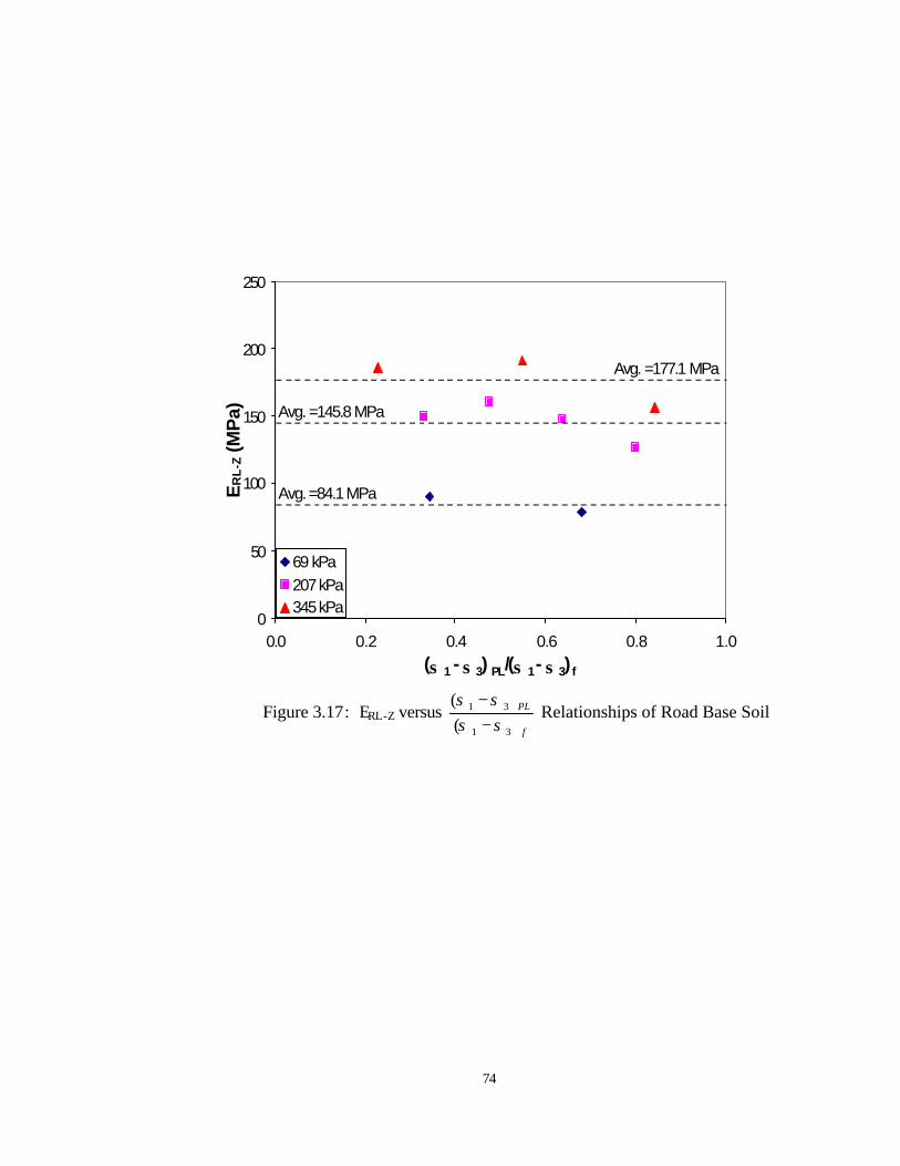
74

Figure 3.17: ERL-Z versus f

PL

)−)−

31

31

((

σσσσ

Relationships of Road Base Soil

0

50

100

150

200

250

0.0 0.2 0.4 0.6 0.8 1.0(σ 1 - σ 3) PL/(σ 1 - σ 3) f

E RL-

Z (M

Pa)

69 kPa207 kPa345 kPa

Avg. =177.1 MPa

Avg. =145.8 MPa

Avg. =84.1 MPa

75

Figure 3.18: ERL-PS versus f

PL

)−)−

31

31

((

σσσσ

Relationships of Road Base Soil

0

50

100

150

200

250

300

0.0 0.2 0.4 0.6 0.8 1.0

(σ 1 - σ 3) PL/(σ 1 - σ 3) f

E RL-

PS (M

Pa)

69 kPa207 kPa345 kPa

Avg. =248.3 MPa

Avg. =207.8 MPa

76

Figure 3.19: Deformation Modulus Versus Confining Pressure Relationships of Ottawa Sand

0

50

100

150

200

250

300

350

400

0 50 100 150 200 250 300 350 400Confining Pressure (kPa)

Defo

rmat

ion

Mod

ulus

(MPa

)

E(50)E(RL-Z)E(RL-PS)

77

Figure 3.20: Deformation Modulus Versus Confining Pressure Relationships of Road Base Soil

0

50

100

150

200

250

300

0 50 100 150 200 250 300 350 400Confining Pressure (kPa)

Def

orm

atio

n M

odul

us (M

Pa)

E(50)E(RL-Z)E(RL-PS)

78

Figure 3.21: p-q Diagram at Failure of Ottawa Sand

0

200

400

600

800

1000

0 200 400 600 800 1000

p = (σ1 + σ3) / 2 (kPa)

q =

( σ1- σ

3)/2

(kPa

)

Monotonic Loading TestsUnloading-Reloading Tests

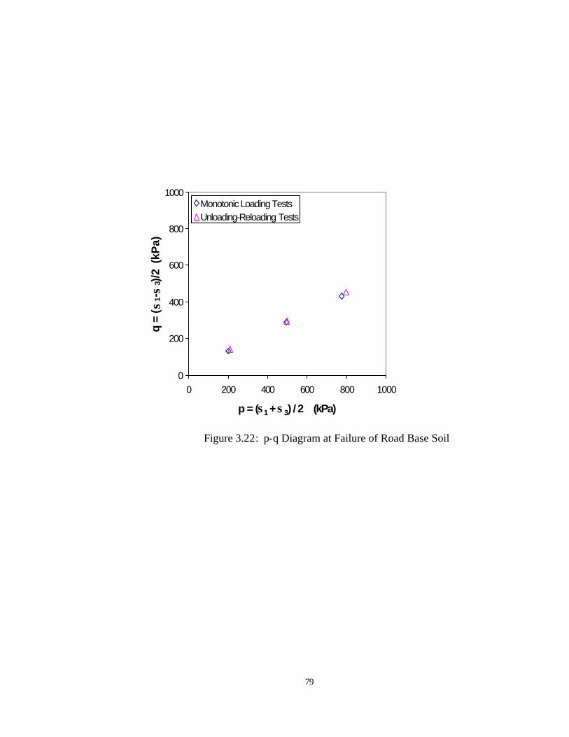
79

Figure 3.22: p-q Diagram at Failure of Road Base Soil

0

200

400

600

800

1000

0 200 400 600 800 1000

p = (σ1 + σ3) / 2 (kPa)

q =

( σ1- σ

3)/2

(kPa

)

Monotonic Loading TestsUnloading-Reloading Tests

80

3.5 In-Isolation Load-Extension Tests for Geosynthetics A series of LE tests under monotonic loading and unloading-reloading cycles was conducted on the two geosynthetics described in Section 3.1.2. The purposes of the tests were to examine the behavior of the geosynthetics subject to unloading-reloading cycles and to calibrate geosynthetic model parameters in the finite element analysis and the SPR model (Sections 5.4 and 6.3).

3.5.1 Test Description

In the LE test, a geosynthetic specimen was subjected to uniaxial tensile force without soil confinement (i.e., in-isolation test). The in-isolation load-extension test is an “element” test. In an element test of geosynthetics, the specimen is subjected to a uniform stress-deformation condition and, as a result, can be considered independent of the specimen dimensions. The in-isolation load-extension tests were conducted in both strain-controlled and stress-controlled modes of loading. All tests were carried out using the MTS-810 testing system.

3.5.2 Specimen Preparation and Test Procedure

The test method specified by ASTM D4595, the wide-width tensile test, uses a 200-mm wide specimen with a gauge length (length between the opposing grips) of 100-mm. The specimen is subjected to a uniaxial tensile force at a constant strain rate of 10% per minute by using a pair of grips that cover the entire width of the test specimen. Yamauchi (1988) showed that the aspect ratio (the ratio of width to gauge length) of 2 in the ASTM wide-width tensile test produced a significant Poisson effect (i.e., necking) in nonwoven geotextiles and gave a weaker load-deformation response. In this study, the geosynthetic specimen for Typar 3301 was 305 mm in width and 25 mm in gauge length. The grip portion was treated with a high strength epoxy (Unitex Propoxy A and B). A schematic diagram of the test specimen for Typar 3301 is shown in Figure 3.23. After sample treatment, the test specimen was fixed to a pair of rigid grips attached to the MTS-810 loading device (see Figure 3.24). The grips consisted of two angle-shaped steel bases that were connected to the MTS-810 loading device and two 25-mm by 38-mm by 305-mm rectangular steel bars. Before the test started, a pretension load of 45 N was applied, per ASTM D4595.

For Amoco 2044, the epoxy-treated grip used in Typar 3301 was not sufficiently stiff to prevent slippage in the grip portion upon tensile load applications. Several gripping methods were examined. The wrapped-around gripping method was selected. The Amoco 2044 specimen was 200 mm in width and 100 mm in gauge length, per ASTM D4595, as shown in Figure 3.25. The overall length of the Amoco 2044 specimen was 480 mm to accommodate the wrapped-around gripping method. The grip portion was treated with high-strength epoxy and two steel plates. The test specimen was wrapped around the rectangular steel bar, as shown in Figure 3.26. A

81

pretension tensile load of 220 N was applied, per ASTM D4595, before starting the test.

3.5.3 Measurement and Test Data Reduction

For Typar 3301 specimens, the elongation and the applied tensile load were measured by the data acquisition system of the MTS-810 loading system. For Amoco 2044 specimens, partial slippage occurred in the grip area. This is known as the end-effect. To eliminate the end-effect in the elongation measurement, a special technique was developed in this study that is described in the following paragraph.

Two rows of small angles (25 mm x 25 mm) were first glued on one side of the specimen marking 100-mm gauge length on prescribed locations as shown in Figure 3.26. Four LVDTs were then mounted on the top of the gripping system. The stylus of each LVDT was in contact with the angle that was glued on the specimen. Elongation of the specimen was the change in distance between the two angles that were vertically aligned. The average elongation of two angle sets was used to calculate the axial strain. The LVDT readings were recorded by the DATAQ4500 data acquisition system. The sensitivity of the LVDT was +0.005 mm. The applied tensile load was recorded by the data acquisition system of the MTS-810 loading system.

The tensile load per unit length (T) and the axial strain of the specimen (εa) were calculated by the following formulas:

oWPT = [3.5]

Oa L∆Lε = [3.6]

where P = applied axial load (in tension) Wo = initial width of the specimen

(305 mm for Typar 3301 specimen and 200 mm for Amoco 2044 specimen)

∆L = elongation of the specimen Lo = gauge length

(25 mm for Typar 3301 specimen and 100 mm for Amoco 2044 specimen)

82

Figure 3.23: Typar 3301 Specimen

305 mm

25 mm

83

Figure 3.24: LE Test Setup for Typar 3301 Specimen

Typar 3301 Specimen

(a) Front View (b) Side View

84

Figure 3.25: Amoco 2044 Specimen

Gage length = 100 mm

200 mm

480 mm

305 mm

85

Figure 3.26: LE Test Setup for Amoco 2044 Specimen

Amoco 2044Specimen

LVDT

Steel Angle

Steel Angle

LVDT

(a) Front View (b) Side View

86

4.5.4 Test Programs The test programs for the LE tests are presented in Table 3.4 for Typar 3301

and Table 3.5 for Amoco 2044. The test program was divided into two groups: monotonic (M) tests and unloading-reloading (UR) tests. Designations of all the tests are shown in the tables. The monotonic tests were conducted in a strain-controlled mode at a constant strain rate of 10% per minute. The unloading-reloading (UR) tests were conducted in a stress-controlled mode with various loading sequences at a constant loading rate of 1.75 kN/m per minute, followed by a strain-controlled mode at a constant strain rate of 10% per minute up to failure.

87

Table 3.4: LE Test Program for Typar 3301

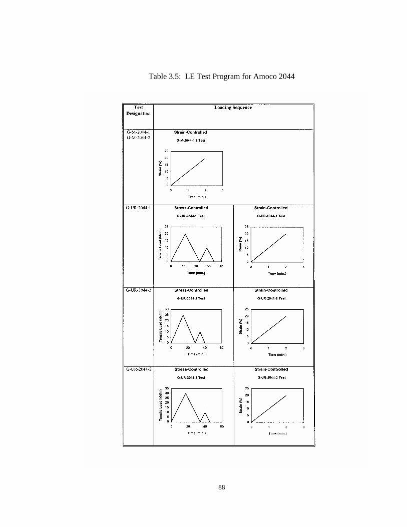
88

Table 3.5: LE Test Program for Amoco 2044

89

3.5.5 Test Results and Discussions The LE test results and discussions of the test results are presented in the

following sections. The general behavior was first described, followed by an assessment of the effects of preloading on deformation and tensile strength of the geosynthetics.

3.5.5.1 General Behavior To describe the load-deformation behavior of the geosynthetics, an ultimate tensile load (TULT) is defined. The ultimate tensile load is defined as either the actual peak tensile load or, if the tensile load continued to increase during the test, the tensile load at 100% axial strain. Figures 3.27 and 3.28 present the tensile load versus axial strain relationships of the monotonic-loading LE tests of Typar 3301 and Amoco 2044, respectively. The ultimate tensile load of Typar 3301 was 7.0 kN/m at 100% axial strain without experiencing rupture failure. For Amoco 2044, two identical specimens were used for Test G-M-2044 to evaluate the gripping method and the new elongation measurement technique described in Section 3.5.2. As shown in Figure 3.28, the load-strain curves are almost identical before failure. The ultimate tensile loads of Specimens 1 and 2 were 67 kN/m and 72 kN/m, with a rupture failure along the center line of the specimen. The average ultimate tensile load was 69.5 kN/m. The tensile load at 5% strain was 36 kN/m. The ultimate tensile load and tensile load at 5% strain, as provided by the manufacturer, are 70 kN/m and 38 kN/m, respectively. The gripping system is considered adequate for the LE test of Amoco 2044 geotextile. The results of stress-controlled and strain-controlled parts of the unloading-reloading LE test are presented separately. The stress-controlled part was presented first. The result of the monotonic-loading LE test was superimposed in the load-strain plot of the strain-controlled response for comparison.

Figures 3.29 to 3.32 show the tensile load versus axial strain relationships of the unloading-reloading LE tests. Figures 3.29 and 3.30 are, respectively, the results of the stress-controlled and strain-controlled parts of Typar 3301. Figures 3.31 and 3.32 are, respectively, the results of the stress-controlled and strain-controlled parts of Amoco 2044. In the stress-controlled part, the specimen was loaded under a loading rate of 1.75 kN/m per minute up to a preloading level, unloaded, and reloaded to 2 kN/m for Typar 3301 and 10 kN/m for Amoco 2044, then unloaded. The specimen was subsequently subjected to a monotonic loading at a strain rate of 10% per minute (strain-controlled part) until failure occurred.

From the results of the stress-controlled part, it is seen that the load-strain relationships of the primary loading, unloading, and reloading were non-linear. The irrecoverable strain occurred upon unloading. The hysteresis loop existed during unloading and reloading.

90

The initiation point of the load-strain curve in the strain-controlled part was the irrecoverable strain of the stress-controlled part. The slope of the reloading curve changed significantly once the tensile load reached the preloading load level. The load-strain curve resembled the monotonic-loading curve after the tensile load exceeded the preloading load level. 3.5.5.2 Effects of Preloading on Elongation and Tensile Strength of Geosynthetics

The secant stiffness is introduced to examine the effects of preloading on deformation of the geosynthetics used in this study. The secant stiffness is defined as the secant slope of a tensile load-strain curve at a given tensile load. The secant stiffness was determined at the tensile load of 2 kN/m for Typar 3301 and 10 kN/m for Amoco 2044. The secant stiffness from the preloading path was 44.2 kN/m for Typar 3301 and 625 kN/m for Amoco 2044. The secant stiffness from the preloading path was used as a reference to calculate the stiffness ratio. The stiffness ratio is the ratio of the secant stiffness determined from the preloading and reloading load-strain curves at the same tensile load.

Figure 3.33 shows the stiffness ratio versus ULT

PL

TT relationships of Typar 3301

and Amoco 2044. The ratioULT

PL

TT is an indication of the relative magnitude of

preloading load level. The stiffness ratio of Typar 3301 and Amoco 2044 appeared to

reduce with increasing preloading load levels. The stiffness ratios at ULT

PL

TT = 0.43,

0.5, and 0.71 were, respectively, 1.7, 1.2, and 0.8 for Typar 3301. The stiffness ratios

at ULT

PL

TT = 0.29, 0.36, and 0.43 were, respectively, 2.3, 1.2, and 1.2 for Amoco 2044.

This behavior indicates that preloading can have a detrimental effect on the geosynthetics if the preloading level exceeds a certain critical load level. For Typar 3301 and Amoco 2044, the threshold load level was about half of the ultimate tensile load. Figure 3.34 shows failure load ratio versus TPL/TULT relationships of Typar 3301 and Amoco 2044. The failure load ratio was the ratio of ultimate loads of the preloaded specimen and the corresponding virgin specimen. It is shown that preloading reduced the ultimate load of the geosynthetics by about 5%.

91

Figure 3.27: Tensile Load Versus Axial Strain Relationship, Test G-M-3301

Figure 3.28: Tensile Load Versus Axial Strain Relationships, Tests G-M-2044-1, 2

0

1

2

3

4

5

6

7

8

0 20 40 60 80 100 120

Axial Strain (%)

Tens

ile L

oad

(kN

/m)

0

10

20

30

40

50

60

70

80

0 2 4 6 8 10 12 14 16

Axial Strain (%)

Tens

ile L

oad

(kN

/m)

G-M-2044-1G-M-2044-2

92

Figure 3.29: Tensile Load Versus Axial Strain Relationships of Tests G-UR-3301-1, 2, and 3 (Stress-Controlled Part)

0

1

2

3

4

5

6

7

8

0 10 20 30 40 50

Axial Strain (%)

Tens

ile L

oad

(kN

/m) (a) Test G-UR-3301-1

0

1

2

3

4

5

6

7

8

0 10 20 30 40 50Axial Strain (%)

Tens

ile L

oad

(kN

/m) (b) Test G-UR-3301-2

0

1

2

3

4

5

6

7

8

0 10 20 30 40 50

Axial Strain (%)

Tens

ile L

oad

(kN

/m) (c) Test G-UR-3301-3

93

Figure 3.30: Tensile Load Versus Axial Strain Relationships of Test G-M-3301 and Tests G-UR-3301-1, 2, 3 (Strain-Controlled Part)

0

1

2

3

4

5

6

7

8

0 20 40 60 80 100 120

Axial Strain (%)

Tens

ile L

oad

(kN

/m)

G-M-3301G-UR-3301-1G-UR-3301-2G-UR-3301-3

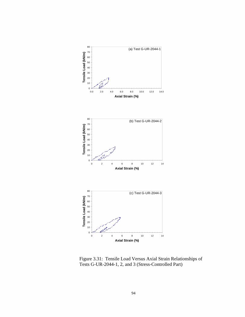
94

Figure 3.31: Tensile Load Versus Axial Strain Relationships of Tests G-UR-2044-1, 2, and 3 (Stress-Controlled Part)

0

10

20

30

40

50

60

70

80

0.0 2.0 4.0 6.0 8.0 10.0 12.0 14.0

Axial Strain (%)

Tens

ile L

oad

(kN

/m)

(a) Test G-UR-2044-1

0

10

20

30

40

50

60

70

80

0 2 4 6 8 10 12 14

Axial Strain (%)

Tens

ile L

oad

(kN

/m)

(b) Test G-UR-2044-2

0

10

20

30

40

50

60

70

80

0 2 4 6 8 10 12 14

Axial Strain (%)

Tens

ile L

oad

(kN

/m)

(c) Test G-UR-2044-3

95

Figure 3.32: Tensile Load Versus Axial Strain Relationships of Test G-M-2044-1 and Tests G-UR-2044-1, 2 (Strain-Controlled Part)

0

10

20

30

40

50

60

70

80

0 2 4 6 8 10 12 14

Axial Strain (%)

Tens

ile L

oad

(kN

/m)

G-M-2044-1G-UR-2044-1G-UR-2044-2

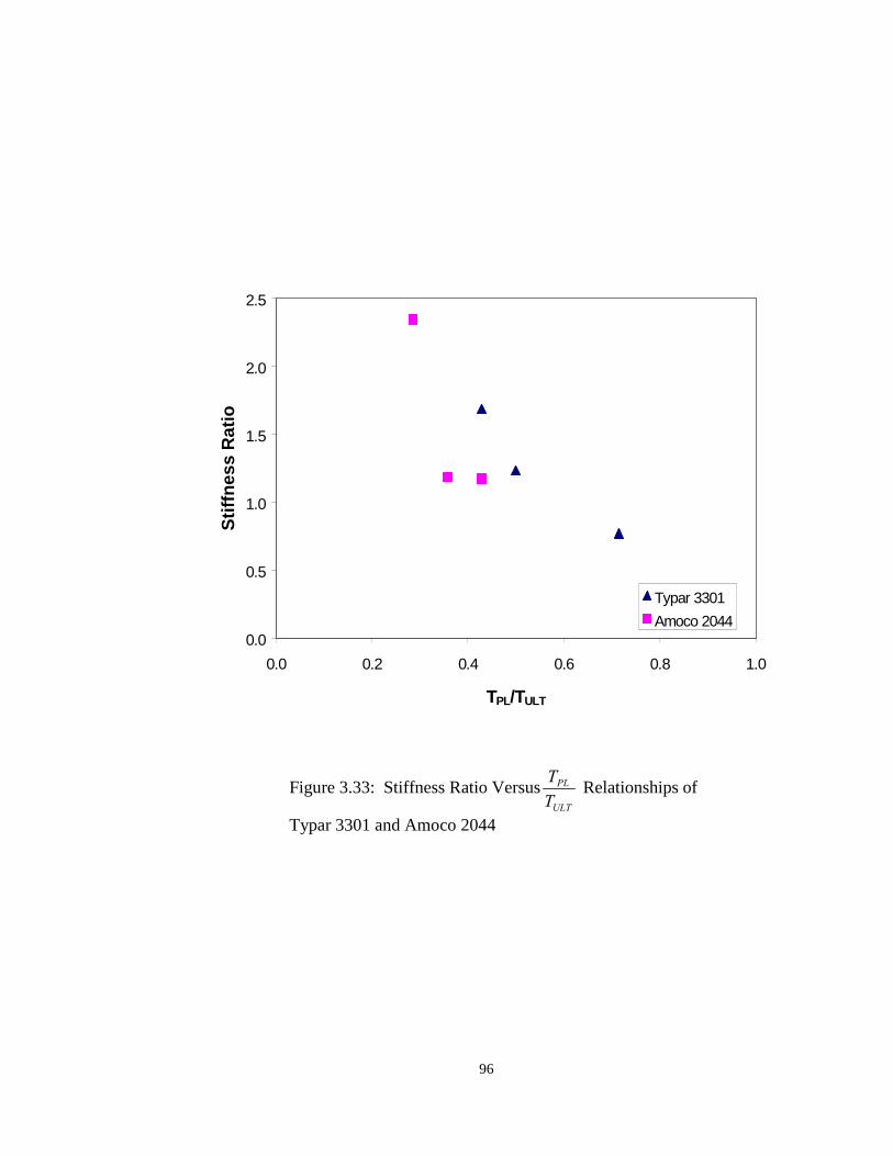
96

Figure 3.33: Stiffness Ratio VersusULT

PL

TT Relationships of

Typar 3301 and Amoco 2044

0.0

0.5

1.0

1.5

2.0

2.5

0.0 0.2 0.4 0.6 0.8 1.0

TPL/TULT

Stiff

ness

Rat

io

Typar 3301Amoco 2044

97

Figure 3.34: Failure Load Ratio VersusULT

PL

TT Relationships of Typar 3301

and Amoco 2044

0.50

0.75

1.00

1.25

1.50

0.0 0.2 0.4 0.6 0.8 1.0

TPL/TULT

Failu

re L

oad

Rat

io

Typar 3301Amoco 2044

98

3.6 Direct Shear Tests for Soil-Geosynthetic Interfaces A series of DS tests on the soil-geosynthetic interfaces was conducted under

monotonic loading and unloading-reloading cycles. The purposes of the tests were to examine the behavior of the interfaces subject to unloading-reloading cycles and to calibrate interface model parameters in the finite element analysis and the SPR model (Sections 5.4 and 6.3).

3.6.1 Test Description

The DS test apparatus consisted of a pair of 60-mm by 60-mm by 20-mm deep shear boxes with a displacement-controlled loading system. The rate of shear displacement was 0.4 mm per minute. The constant normal stress was applied by a dead load.

A geotextile specimen with dimensions of 60 mm x 60 mm was firmly glued to the top surface of a rigid wooden block. The wooden block with the geosynthetic specimen was placed inside the lower shear box. The thickness of the wooden block was modified several times to have the geosynthetic surface positioned at 0.1 mm above the horizontal surface of the lower shear box. The soil was placed in the upper shear box.

The unloading and reloading paths of the DS test were manually controlled by reversal of the upper box displacement. In the preloading path, the upper box moved in one direction until a preloading shear stress level was reached. The movement direction of the upper box was then reversed to represent the unloading path. When the reversed shear stress in the unloading path was equal to the magnitude of the preloading shear stress level, the movement direction was reversed again to represent the reloading path. The size of the DS test in this study was relatively small. The boundary effects could affect the test results to some degree. However, the test results with the 60-mm-square direct shear box were expected to have insignificant boundary effects for two reasons. First, the dimensions of the direct shear box were approximately 100 times the mean grain size (D50) of the soil specimen. This was in the range recommended by ASTM D3080 and by other researchers (Jewell and Wroth, 1987; Palmeira, 1988). Second, it was confirmed by O’Rourke et al. (1990) that the 60-mm-square direct shear apparatus for Ottawa sand and HDPE gave results similar to those obtained from larger size direct shear apparatus. O’Rourke et al. (1990) conducted a series of direct shear tests on Ottawa sand and HDPE using a 60-mm- square shear box. They compared the test results with those obtained by using different sizes of direct shear boxes by Martin et al. (1984), Saxena and Wong (1984), and Williams and Houlihan (1987). It was found that all the direct shear test results were similar.

99

The DS tests were conducted on the interfaces between the Ottawa sand and Amoco 2044, and between the Road Base soil and Amoco 2044. The DS tests results of Typar 3301 and the Ottawa sand were readily available from Wu (1993). 3.6.2 Specimen Preparation and Test Procedure

The specimen preparation and the test procedure of the interface tests are as follows:

1. Glue a 60-mm x 60-mm geosynthetic sheet on the top surface of a rigid wooden block.

2. Fit the rigid wooden block with the geosynthetic sheet inside the lower direct shear box.

3. Place the upper shear box on top of the lower shear box and tighten corner screws.

4. Place soil in the upper shear box. For the Road Base soil, the soil was compacted in the upper shear box by tamping. The Road Base soil used in the direct shear tests was minus #4 standard sieve material with a water content of 12.2%. For the Ottawa sand, the sand was poured in the upper shear box and densified to a prescribed density by vibrating the direct shear box.

5. Place a rigid loading plate on top of the soil. 6. Remove the corner screws and lift the upper shear box up to have a 0.5 mm

gap between the lower and upper shear boxes. 7. Apply a constant vertical load on the rigid loading plate. 8. Allow the specimen to compress until the vertical movement cease or

becomes negligible. 9. Mount two LVDTs to measure the vertical movement of the rigid loading

plate and the horizontal applied load. 10. Apply horizontal loads in a constant displacement mode.

3.6.3 Measurement and Test Data Reduction The vertical deformation of the test specimen was recorded by an LVDT

(sensitivity = +0.005 mm). The applied shear force was measured by the other LVDT (sensitivity = +8 N) attached to a proof ring. The LVDT measurement has been calibrated with the proof ring gauge to obtain the relationship between the LVDT displacement and the horizontal load. The LVDTs were connected to a DATAQ4500 data acquisition system. The horizontal movement of the upper box was calculated from the controlled displacement rate and time. The shear stress (τ.) along the soil-geosynthetic interface was calculated from the following formula:

O

h

AF

t = [3.7]

100

where Fh = applied horizontal force

Ao = horizontal cross-sectional area of the specimen (assumed to be constant and equal to the initial area)

3.6.4 Test Programs

Test programs for the DS tests are presented in Table 3.6 for the Ottawa sand and Amoco 2044 interface and Table 3.7 for the Road Base soil and Amoco 2044 interface. The test program was divided into two groups: monotonic-loading (M) tests and unloading-reloading (UR) tests. The monotonic- loading and unloading-reloading tests were conducted in a displacement-controlled mode at a constant displacement rate of 0.4 mm per minute.

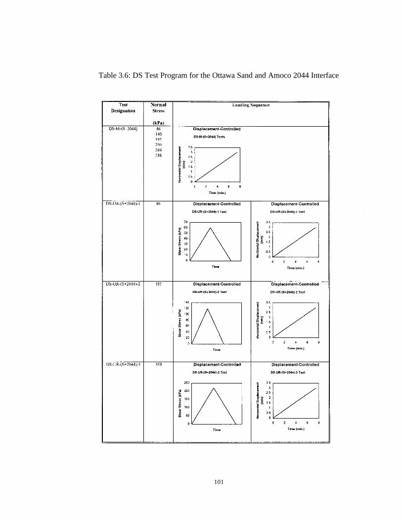
101

Table 3.6: DS Test Program for the Ottawa Sand and Amoco 2044 Interface

102

Table 3.7: DS Test Program for the Road Base Soil and Amoco 2044 Interface

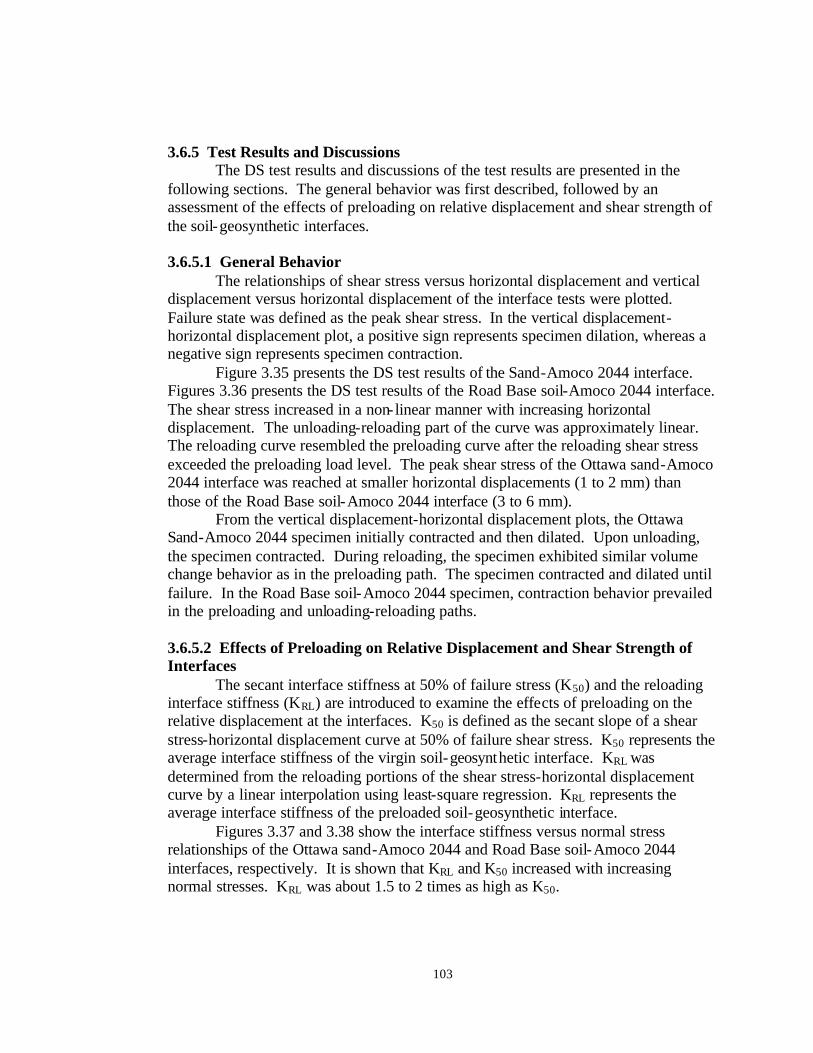
103

3.6.5 Test Results and Discussions The DS test results and discussions of the test results are presented in the

following sections. The general behavior was first described, followed by an assessment of the effects of preloading on relative displacement and shear strength of the soil-geosynthetic interfaces.

3.6.5.1 General Behavior

The relationships of shear stress versus horizontal displacement and vertical displacement versus horizontal displacement of the interface tests were plotted. Failure state was defined as the peak shear stress. In the vertical displacement-horizontal displacement plot, a positive sign represents specimen dilation, whereas a negative sign represents specimen contraction.

Figure 3.35 presents the DS test results of the Sand-Amoco 2044 interface. Figures 3.36 presents the DS test results of the Road Base soil-Amoco 2044 interface. The shear stress increased in a non- linear manner with increasing horizontal displacement. The unloading-reloading part of the curve was approximately linear. The reloading curve resembled the preloading curve after the reloading shear stress exceeded the preloading load level. The peak shear stress of the Ottawa sand-Amoco 2044 interface was reached at smaller horizontal displacements (1 to 2 mm) than those of the Road Base soil-Amoco 2044 interface (3 to 6 mm).

From the vertical displacement-horizontal displacement plots, the Ottawa Sand-Amoco 2044 specimen initially contracted and then dilated. Upon unloading, the specimen contracted. During reloading, the specimen exhibited similar volume change behavior as in the preloading path. The specimen contracted and dilated until failure. In the Road Base soil-Amoco 2044 specimen, contraction behavior prevailed in the preloading and unloading-reloading paths.

3.6.5.2 Effects of Preloading on Relative Displacement and Shear Strength of Interfaces

The secant interface stiffness at 50% of failure stress (K50) and the reloading interface stiffness (KRL) are introduced to examine the effects of preloading on the relative displacement at the interfaces. K50 is defined as the secant slope of a shear stress-horizontal displacement curve at 50% of failure shear stress. K50 represents the average interface stiffness of the virgin soil-geosynthetic interface. KRL was determined from the reloading portions of the shear stress-horizontal displacement curve by a linear interpolation using least-square regression. KRL represents the average interface stiffness of the preloaded soil-geosynthetic interface. Figures 3.37 and 3.38 show the interface stiffness versus normal stress relationships of the Ottawa sand-Amoco 2044 and Road Base soil-Amoco 2044 interfaces, respectively. It is shown that KRL and K50 increased with increasing normal stresses. KRL was about 1.5 to 2 times as high as K50.

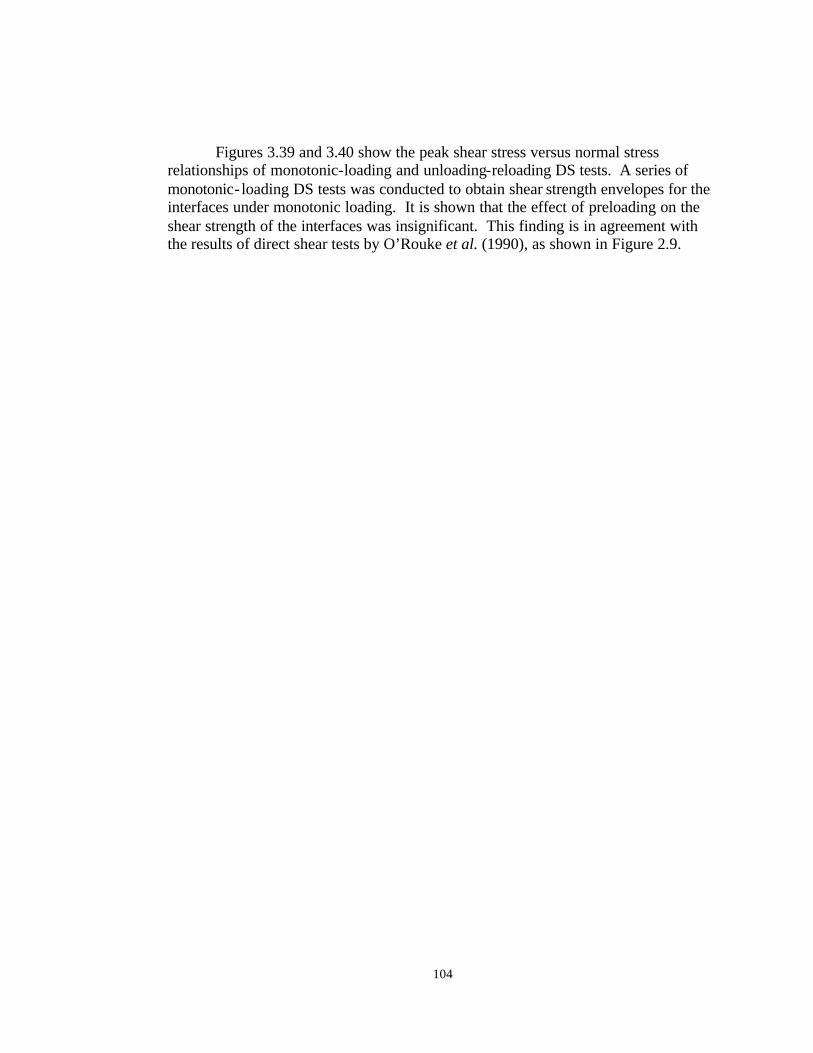
104

Figures 3.39 and 3.40 show the peak shear stress versus normal stress relationships of monotonic-loading and unloading-reloading DS tests. A series of monotonic- loading DS tests was conducted to obtain shear strength envelopes for the interfaces under monotonic loading. It is shown that the effect of preloading on the shear strength of the interfaces was insignificant. This finding is in agreement with the results of direct shear tests by O’Rouke et al. (1990), as shown in Figure 2.9.

105

Figure 3.35: Results of Tests DS-UR-(S+2044)-1, 2, and 3

0

50

100

150

200

250

300

0 0.5 1 1.5 2 2.5 3 3.5

Horizontal Displacement (mm)

Shea

r Stre

ss (k

Pa)

195 kPa

358 kPa

86 kPa

-0.1

-0.05

0

0.05

0.1

0.15

0.2

0.25

0.3

0 0.5 1 1.5 2 2.5 3 3.5Horizontal Displacement (mm)

Vert

ical

Dis

plac

emen

t (m

m)

86 kPa195 kPa

358 kPa

106

Figure 3.36: Results of Tests DS-UR-(RB+2044)-1, 2, and 3

0

50

100

150

200

250

300

0 1 2 3 4 5 6 7

Horizontal Displacement (mm)

Shea

r Stre

ss (k

Pa)

86 kPa

195 kPa

358 kPa

-0.8

-0.7

-0.6

-0.5

-0.4

-0.3

-0.2

-0.1

0

0.1

0 1 2 3 4 5 6 7

Horizontal Displacement (mm)

Vert

ical

Dis

plac

emen

t (m

m) 86 kPa

195 kPa

358 kPa

107

Figure 3.37: Interface Stiffness Versus Normal Stress Relationships of Ottawa Sand and Amoco 2044 Interface

0

50,000

100,000

150,000

200,000

250,000

300,000

350,000

400,000

0 50 100 150 200 250 300 350 400

Normal Stress (kPa)

Inte

rface

Stif

fnes

s (k

N/m

3 )

K(50)K(RL)

108

Figure 3.38: Interface Stiffness Versus Normal Stress Relationships of Road Base Soil and Amoco 2044 Interface

0

50,000

100,000

150,000

200,000

250,000

300,000

350,000

0 50 100 150 200 250 300 350 400

Normal Stress (kPa)

Inte

rfac

e St

iffne

ss (k

N/m

3 )

K(50)K(RL)

109

Figure 3.39: Peak Shear Stress Versus Normal Stress Relationships of Ottawa Sand and Amoco 2044 Interface

0

50

100

150

200

250

300

350

400

0 100 200 300 400

Normal Stress (kPa)

Peak

She

ar S

tress

(kPa

)

Monotonic DS TestsUnloading-Reloading DS TestsLinear (Monotonic DS Tests)

110

Figure 3.40: Peak Shear Stress Versus Normal Stress Relationships of Road Base Soil and Amoco 2044 Interface

0

50

100

150

200

250

300

350

400

0 100 200 300 400

Normal Stress (kPa)

Peak

She

ar S

tres

s (k

Pa)

Monotonic DS TestsUnloading-Reloading DS TestsLinear (Monotonic DS Tests)

111

3.7 Summary and Concluding Remarks Laboratory tests were conducted to examine the behavior of different soils, geosynthetics, and soil-geosynthetic interfaces subject to monotonic loading and unloading-reloading cycle(s). The tests consisted of conventional triaxial compression (CTC) tests for soils, in- isolation load-extension (LE) tests for geosynthetics, and direct shear (DS) tests for soil-geosynthetic interfaces. Each test category employed two types of loading sequence: monotonic loading and unloading-reloading cycle(s). Test specimens used for the monotonic- loading tests were referred to as virgin specimens, whereas test specimens used for the unloading-reloading test were referred to as preloaded specimens. The test results showed that: 1. The stiffness of the soils increased due to preloading. The reloading stiffness was

found to depend on the confining pressure and the unloading load level. At the same confining pressure, the reloading stiffness in the RL-PS path was higher than in the RL-Z path.

2. The stiffness of the preloaded geosynthetic specimen was higher than that of the virgin specimen, provided that the preloading load level was less than about 50% of the ultimate tensile strength. The reloading stiffness reduced with increasing preloading level.

3. The reloading stiffness of the preloaded interface was higher than that of the interface without preloading. The reloading stiffness of the interface increased with increasing normal stress applied on the interface.

4. Preloading did not affect the shear strength of the soils or the interfaces. 5. The tensile strength of the preloaded geosynthetic specimen was about 5% lower

than that of the corresponding virgin specimen.

112

4. SGP Test Apparatus In this study, a modified SGP test apparatus was devised for investigating the behavior of a generic GRS mass subject to monotonic loading and unloading-reloading cycles. The SGP test apparatus was the third generation of a SGP test device developed at the University of Colorado at Denver. Typically, the performance test is performed on a soil-reinforcement composite consisting of soil and horizontally placed layer(s) of geosynthetic reinforcement in a plane strain condition. The geosynthetic reinforcement and the confining soil are allowed to deform in an interactive manner upon load applications. The geosynthetic tensile stresses are induced by the stresses developed in the soil resulting from the self-weight of the soil and externally applied loads.

Conceptually, the SGP test specimen represents neither an element in a prototype GRS structure nor a reduced scale model of any prototype GRS structures. Generally speaking, the measured quantities of the SGP test, such as deformation and reinforcement strain, cannot be correlated directly to a prototype GRS structure. In this study, the results of the SGP test were used to 1) examine the effects of preloading on deformation and strength of a GRS mass, 2) evaluate the benefits of different unloading-reloading cycles, 3) verify a finite element analysis, 4) evaluate the simplified preloading-reloading (SPR) model developed in this study, and 5) develop a methodology to relate the behavior of a preloaded GRS mass to that of a proloaded GRS structure.

This chapter presents development of the modified SGP test, apparatus configurations, specimen preparations, test procedures, instrumentation, and test programs. 4.1 First and Second Generations of SGP Test Apparatus 4.1.1 First-Generation SGP Test Wu and Helwany (1996) developed a soil-geosynthetic performance test to investigate long-term interactive behavior of soil-geosynthetic composites. A schematic diagram of the test device is shown in Figure 4.1, in which a reinforced-soil mass was placed inside a rigid container with transparent plexiglass side walls. The reinforced-soil mass comprised a sheet of geosynthetic reinforcement, two flexible steel plates, and confining soil. The confining soil confined the geosynthetic reinforcement at both top and bottom. The two ends of the geosynthetic reinforcement were securely attached to the two vertical steel plates at their mid-height. The transverse direction of the reinforced-soil mass was fitted between two lubricated plexiglass sidewalls of a rigid container in such a manner that reinforced-soil mass was restrained from movement in the direction perpendicular to the plexiglass sidewalls (i.e., in a plane strain configuration). On the top surface of the confining soil, another sheet of geosynthetic was used to connect the top edge of

113

the vertical steel plates. Upon the application of a surface load, the geosynthetic reinforcement and its confining soil will deform interactively over time. To maintain the plane strain condition throughout the test, the interface adhesion between the rigid plexiglass and the soil was minimized to nearly frictionless. This was accomplished by creating a lubrication layer at the interface of the plexiglass sidewall and the soil. The lubrication layer consisted of a 0.2-mm-thick membrane and a thin layer of silicon grease. This technique was developed at the University of Tokyo by Tatsuoka and his associates and has been used successfully in many property tests, reduced-scale model tests, and full-scale tests (Tatsuoka et al., 1984; Wu, 1992; Ling and Tatsuoka, 1993) 4.1.2 Second-Generation SGP Test Apparatus The second-generation soil-geosynthetic performance test apparatus was developed by Ketchart and Wu (1996). The new apparatus was devised to simplify the sample preparation procedure and load application. A schematic diagram of the long-term performance test apparatus is shown in Figure 4.2. The test specimen was reduced to 300 mm high, 600 mm wide and 300 mm long. The longitudinal direction of the test specimen was in a state of unconfined condition, whereas in the first-generation apparatus it was supported by flexible steel plates. During sample preparation, the longitudinal sides of the reinforced-soil mass were restrained from movement by two moveable plexiglass plates. With the aid of a pair of air cylinders, the moveable plates were released immediately before testing. Thus, the soil-geosynthetic composite was allowed to deform in an unconfined condition along the longitudinal direction. Also, unlike in the first-generation test, the geosynthetic reinforcement at the mid-height was simply laid horizontally without any artificial restraints at the ends. A sustained vertical load was applied to the top surface of the specimen with a self-contained loading mechanism. 4.2 Modified SGP Test Apparatus A schematic diagram of various components of the modified SGP test apparatus is shown in Figure 4.3. The test apparatus was manufactured by the Turner-Fairbank Highway Research Center of the Federal Highway Administration. Figure 4.4 depicts the new SGP test apparatus with a specimen on the MTS-810 loading apparatus. Each of the components is described in the following sections. 4.2.1 Apparatus Configurations

In the modified SGP test, a generic GRS mass was placed inside a rigid container as shown in Figure 4.5. Dimensions of the specimen were designated as W (width), H (height), and D (depth) in the plane strain direction. The dimensions of the SGP test specimen employed in this study were 610 mm (24 in) high, 254 mm (10 in) wide (W), and 565 mm (22.25 in) deep (D). The test specimen comprised a soil with

114

three layers of reinforcement at the bottom, mid-height, and top. The transverse direction (plane strain direction) of the test specimen was fitted between two lubricated acrylic sidewalls of the rigid container. The test specimen was restrained from movement in the direction perpendicular to the sidewalls (i.e., plane strain direction). The longitudinal direction of the test specimen was unrestrained.

The rigid container had two side panels, six transverse bars, and two base plates. The sidewall panel had dimensions of 890 mm by 915 mm. Each side panel consisted of a 13-mm-thick transparent acrylic panel reinforced by 3.2-mm-thick, 50.8-mm-square steel tubes with center to center spacing of 216 mm in both horizontal and vertical directions. The transverse bars were rigidly connected with the sidewalls to form a container, as shown in Figure 4.6. The height of the sidewall panels can be increased to 1090 mm by using sidewall extensions with two additional transverse bars across the top of the sidewall extensions.

Figures 4.7 and 4.8 show, respectively, the plan view and cross section of the modified SGP test apparatus with a test specimen (without reinforcement layers). Figure 4.7 depicts the sidewall panels, transverse bars, extension transverse bar, and horizontal removable panels with horizontal constraint assemblies. Figure 4.8 shows the cross section A-A from the top view. Figure 4.8 depicts, from the bottom up, a lower base plate, an upper base plate, six horizontal removable panels (three on each side) with horizontal constraint configurations, a sidewall panel, six main transverse bars, an extension sidewall panel, and two extension transverse bars. The test specimen was situated on top of the upper base plate. The upper base plate was a 25-mm-thick, 915-mm by 565-mm steel plate. The lower base plate was a 25-mm-thick, 457-mm by 565-mm steel plate with a 25-mm-thick, 150-mm-diameter steel ring at the center (see Figure 4.8). The lower steel plate was placed on the lower actuator-loading rod of the MTS-810 loading device during load applications. The center ring of the lower steel plate was designed to ensure that the vertical load from the actuator-loading rod was applied to the center of the test specimen.

The horizontal removable panel consisted of a 8-mm-thick steel plate reinforced with two vertical and three horizontal 3.2-mm-thick, 25-mm by 50-mm rectangular tubes. The horizontal removable panels were used during specimen preparation. They were set perpendicular to the sidewall panels to form a cuboid space for the specimen.

During the specimen preparation, a horizontal constraint assembly restrained the horizontal removable panels from horizontal movement. The horizontal constraint assembly comprised a 8.5-mm-thick circular plate and a 8-mm-diameter rod threaded through the transverse bar (see Figures 4.7 and 4.8). The threaded rod controlled the horizontal position of the circular plate. The circular plate was set to touch and restrain the horizontal bars of the horizontal removable panel during the specimen preparation. The horizontal removable panels were removed after completing specimen preparation.

115

The modified SGP test apparatus was designed to accommodate specimens with maximum dimensions of 915 mm (36 in) high (H), 508 mm (20 in) wide (W), and 565 mm (22.25 in) deep (D). The dimensions of the SGP test specimen employed in this study were 610 mm (24 in) high, 254 mm (10 in) wide (W), and 565 mm (22.25 in) deep (D). Note that the depth of the specimen was limited by the clearance of the MTS-810 loading frame. The main factors used to determine the overall specimen dimensions are as follows: 1. Backfill Particle Size: To reduce the particle size effects, the dimensions of a generic GRS mass should be at least 6 times larger than the maximum particle size of the soil specimen, as suggested by the U.S. Army Corps of Engineers, and 15 times larger than the average particle size (D50) (Jewell,1993). The recommended maximum particle size for the backfill of GRS structures is 19 mm (Elias and Christopher, 1996). The specimen dimension, therefore, should be at least 120 mm.

2. Reinforcement Spacing: The reinforcement spacing plays an important role in the deformation behavior of GRS structures (Adams, 1999) and the load-transfer mechanism of reinforced-soil masses (Abramento and Whittle, 1993). The height (H) of a generic GRS mass should be able to accommodate the typical reinforcement spacing with the recommended maximum spacing of 800 mm (Elias and Christopher, 1996).

3. Size of Reinforcement Sheet: The specimen depth in plane strain direction (D) and the specimen width (W) should be large enough to accommodate typical geosynthetic reinforcement (e.g., polymer grids, woven and non-woven geotextiles). Ideally, the reinforcement size used in the SGP test should represent a “very large” sheet of reinforcement. For polymer grids, enough grid “cells” are required for a good representation of the polymer grid specimen. For non-woven geotextiles, the aspect ratio of the reinforcement specimen (i.e., the ratio of width to length) should be at least 2 to alleviate significant necking effects. 4.2.2 Boundary Conditions

The transverse direction (plane strain direction) of the test specimen was fitted between two lubricated acrylic sidewalls of the rigid frame. The test specimen was restrained from movement in the direction perpendicular to the sidewalls (i.e., plane strain condition). The longitudinal direction of the test specimen was unrestrained. On the top of the specimen was a rigid loading plate. The vertical load was applied on the rigid loading plate by the MTS-810 testing system.

All contacted surfaces of the specimen with the SGP test apparatus and the rigid loading plate were lubricated to minimize the interface friction. The lubrication layer consisted of a 0.5-mm-thick latex membrane and a thin layer of silicone grease.

The specimen surface was vacuum-sealed with a 0.5-mm-thick rubber membrane for confining pressure application. The confining pressure was applied by vacuuming. A small-diameter flexible plastic tube connected to a suction machine

116

was attached to one unrestrained side of the specimen (see Figure 4.4). The maximum confining pressure that can be applied by such a system is the atmospheric pressure. The applied confining pressure was controlled by a gauge connected to a suction machine.

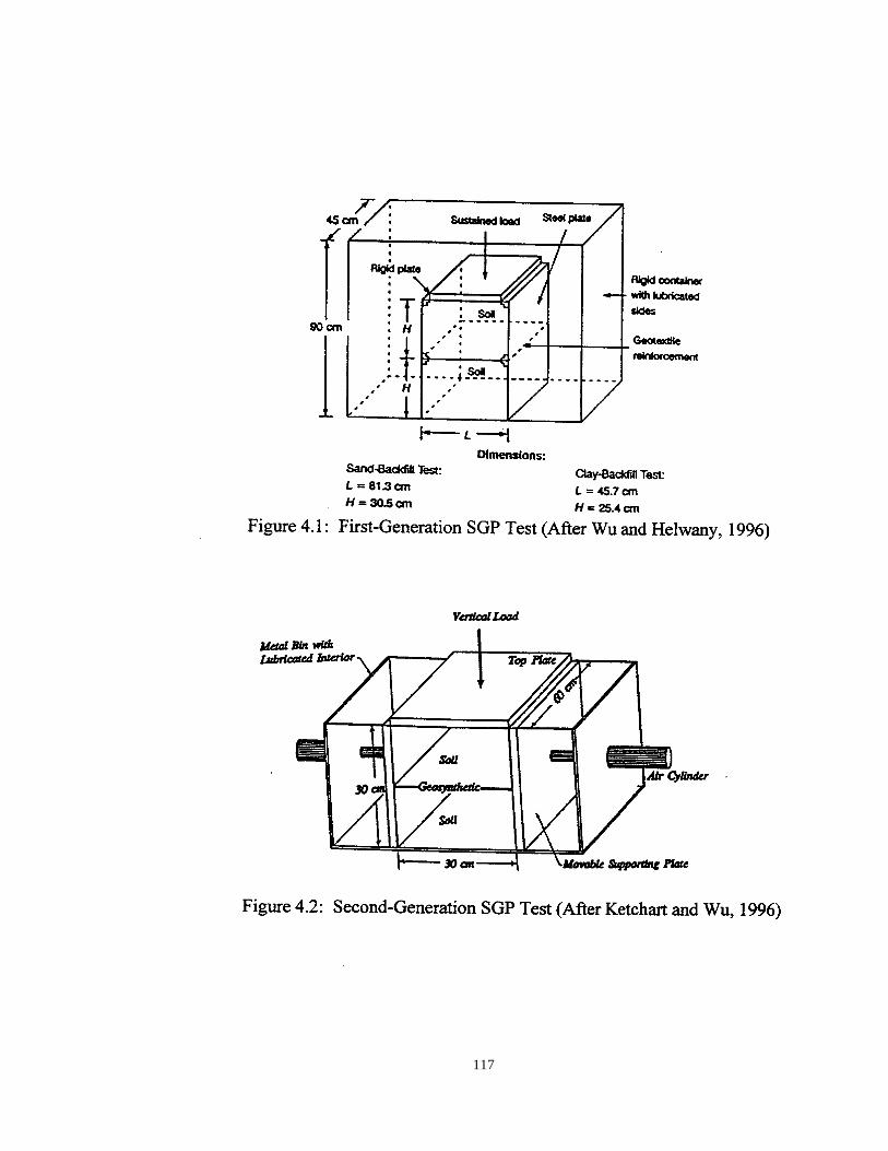
117

118

119

Figure 4.4: Modified SGP Test Apparatus on MTS-810 Loading System Before Testing

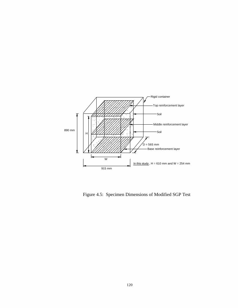
120

Figure 4.5: Specimen Dimensions of Modified SGP Test

Base reinforcement layer

Soil

Soil

Middle reinforcement layer

Top reinforcement layer

D = 565 mm

H

W

Rigid container

915 mmIn this study , H = 610 mm and W = 254 mm

890 mm

121

Figure 4.6: Rigid Container of Modified SGP Test Apparatus

122

1 = Horizontal Constraint 2 = Reinforced Steel Tube 3 = Transparent Acrylic Panel 4 = Horizontal Removable Panel 5 = Extension Transverse Bar 6 = Transverse Bar Figure 4.7: Top View of Modified SGP Test Apparatus

5

6

4321

123

Figure 4.8: Cross Section of Modified SGP Test Apparatus (Section A-A)

1 = Extension Transverse Bar 2 = Extension Side Wall Panel 3 = Side Wall Panel 4 = Transverse Bar 5 = Horizontal Removable Panel

6 = Upper Base Plate 7 = Lower Base Plate

7 6

1

2

3

4TEST

SPECIMEN

5

124

4.2.3 Specimen Preparation and Test Procedure 4.2.3.1 Sand Specimen

The sand was placed inside the modified SGP test apparatus at a constant density of 16.85 kN/m3 (+0.5 kN/m3) by an air-pluviation method using a hopper designed for construction of the Denver wall (Wu, 1993). The hopper dispensed sand uniformly as it traveled in a pendulum motion over the SGP test apparatus (see Figure 4.9). During specimen preparation, the hopper was raised incrementally as the specimen height increased to ensure a constant height of pluviation. The opening size of the hopper is adjustable by a linkage control attached to the handle of the hopper.

Factors affecting the sand density in the air-pluviation method are the size of opening of the hopper, the height of pluviation, and the swing rate. To achieve the prescribed sand density, a trial-and-error process was employed to determine the appropriate opening size, the height of pluviation, and the swing rate of the hopper. The sand was dispensed from the hopper into two 100-mm-diameter Proctor molds placed 80 mm apart at the various opening sizes, heights of pluviation, and swing rates. It was found that the sand density decreased with the increase of the opening size and the swing rate and increased with the increase of the height of pluviation. In this study, the opening size of 2 mm, the height of pluviation of 1.0 m, and the swing rate of approximately 2 seconds per swing were used to obtain the targeted density.

The rubber membrane used for the sand specimen was prepared prior to sample preparation. The rubber membrane was cut to a special shape and folded to form a 254-mm by 565-mm by 915-mm bag. The edges of the rubber membrane were glued together by a clear silicone sealant.

The specimen preparation and the test procedure for the SGP test with the Ottawa sand are as follows: 1. Lubricate the entire base and sidewall surface areas with a silicone grease. 2. Install the moveable rigid panels to form a cuboid space for the specimen. 3. Apply a thin layer of silicone grease on the inner surfaces of the moveable rigid

panels. 4. Place the rubber membrane bag in the cuboid space of the apparatus. 5. Remove the air bubbles trapped between the rubber membrane and the contacted

surface. 6. Connect the small-diameter vacuuming tube to the rubber membrane. 7. Place the bottom reinforcement layer (for a test with reinforcement). 8. Place a large cardboard with a 254-mm by 565-mm rectangular slot on top of the

apparatus to prevent spilling of the sand outside the cuboid space. 9. Raise the hopper filled with the sand to a prescribed drop height. 10. Start dispersing the sand with a pendulum motion of the hopper. 11. Move the hopper up incrementally to maintain a constant height of pluviation. 12. Place the middle reinforcement layer at mid-height and continue dispersing the

sand until full-height is reached.

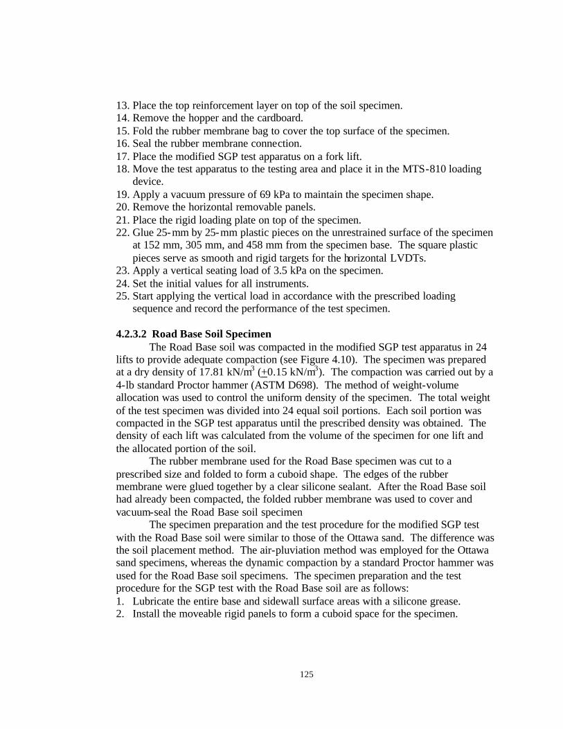
125

13. Place the top reinforcement layer on top of the soil specimen. 14. Remove the hopper and the cardboard. 15. Fold the rubber membrane bag to cover the top surface of the specimen. 16. Seal the rubber membrane connection. 17. Place the modified SGP test apparatus on a fork lift. 18. Move the test apparatus to the testing area and place it in the MTS-810 loading

device. 19. Apply a vacuum pressure of 69 kPa to maintain the specimen shape. 20. Remove the horizontal removable panels. 21. Place the rigid loading plate on top of the specimen. 22. Glue 25-mm by 25-mm plastic pieces on the unrestrained surface of the specimen

at 152 mm, 305 mm, and 458 mm from the specimen base. The square plastic pieces serve as smooth and rigid targets for the horizontal LVDTs.

23. Apply a vertical seating load of 3.5 kPa on the specimen. 24. Set the initial values for all instruments. 25. Start applying the vertical load in accordance with the prescribed loading

sequence and record the performance of the test specimen. 4.2.3.2 Road Base Soil Specimen

The Road Base soil was compacted in the modified SGP test apparatus in 24 lifts to provide adequate compaction (see Figure 4.10). The specimen was prepared at a dry density of 17.81 kN/m3 (+0.15 kN/m3). The compaction was carried out by a 4-lb standard Proctor hammer (ASTM D698). The method of weight-volume allocation was used to control the uniform density of the specimen. The total weight of the test specimen was divided into 24 equal soil portions. Each soil portion was compacted in the SGP test apparatus until the prescribed density was obtained. The density of each lift was calculated from the volume of the specimen for one lift and the allocated portion of the soil.

The rubber membrane used for the Road Base specimen was cut to a prescribed size and folded to form a cuboid shape. The edges of the rubber membrane were glued together by a clear silicone sealant. After the Road Base soil had already been compacted, the folded rubber membrane was used to cover and vacuum-seal the Road Base soil specimen

The specimen preparation and the test procedure for the modified SGP test with the Road Base soil were similar to those of the Ottawa sand. The difference was the soil placement method. The air-pluviation method was employed for the Ottawa sand specimens, whereas the dynamic compaction by a standard Proctor hammer was used for the Road Base soil specimens. The specimen preparation and the test procedure for the SGP test with the Road Base soil are as follows: 1. Lubricate the entire base and sidewall surface areas with a silicone grease. 2. Install the moveable rigid panels to form a cuboid space for the specimen.

126

3. Place rubber membranes over the lubricated base and sidewall areas. 4. Remove the air bubbles trapped between the rubber membrane and the contacted

surface. 5. Place the bottom reinforcement layer (for a test with reinforcement). 6. Start compacting the Road Base soil in 25-mm-thick lifts. 7. Place the middle reinforcement layer at the mid-height and continue compacting

the Road Base soil to full-height. 8. Place the top reinforcement layer on top of the soil specimen. 9. Place the SGP test apparatus on a fork lift. 10. Move the test apparatus to the testing area and place it in the MTS-810 loading

device. 11. Remove the horizontal removable panels. 12. Cover and vacuum-seal the specimen with the pre-prepared rubber membrane. 13. Connect the vacuuming tube to the rubber membrane. 14. Apply a vacuum pressure of 34.5 kPa. 15. Place the rigid loading plate on top of the specimen. 16. Glue 25-mm by 25-mm plastic pieces on the unrestrained surface of the specimen

at 152 mm, 305 mm, and 458 mm from the specimen base. The square plastic pieces serve as smooth and rigid targets for the horizontal LVDT.

17. Apply a vertical seating load of 3.5 kPa on the specimen. 18. Set the initial values for all instruments. 19. Start applying the vertical load in accordance with the prescribed loading

sequence and record the performance of the test specimen. 4.2.4 Instrumentation

The instrumentation layout for the modified SGP test is shown in Figure 4.3. The vertical deformation of the specimen (i.e., vertical displacement of the rigid loading plate) and the applied vertical load were measured by the internal LVDT and the load cell, respectively, of the data acquisition system of the MTS-810 loading system. A total of six LVDTs (three on each side) were used to measure the horizontal deformation of the specimen in the direction perpendicular to the plane strain direction. Three LVDTs were installed on each side of the specimen at 152 mm (point B, Figure 4.3), 305 mm (point M, Figure 4.3), and 458 mm (point T, Figure 4.3) from the base or at ¼, ½, and ¾ points of the specimen height. The sensitivity of the horizontal LVDT was +0.005mm. In one test with the Road Base soil and Amoco 2044 reinforcement, nine strain gauges were mounted on the middle reinforcement layer (see Figure 4.11). The gauges were installed to measure strains in the fill direction of the reinforcement, which was oriented perpendicular to the plane strain direction.

The strain gauges were mounted by a “patch” procedure. A strain gauge was first mounted on a 25-mm x 76-mm patch. The patch was a weak heat-bonded non-

127

woven geotextile. Each strain gauge was glued to the geotextile patch only at the two ends to avoid inconsistent local stiffening of the geotextile because of adhesive (Billiard and Wu, 1991). The geotextile patch (with a strain gauge mounted) was then attached to the geotextile reinforcement at a prescribed location. A microcrystalline wax and a Neoprene rubber patch were applied over the gauge to protect it from soil moisture and possible mechanical damage during compaction and during testing. Due to the presence of the lightweight geotextile patch, calibration was needed. A wide-width tensile test was performed to correlate the recorded strains to actual strains of the geotextile reinforcement. Figure 4.12 shows the wide-width tensile test performed on the Amoco 2044 specimen with two strain gauges mounted on one side. The calibration curves are shown in Figure 4.13.

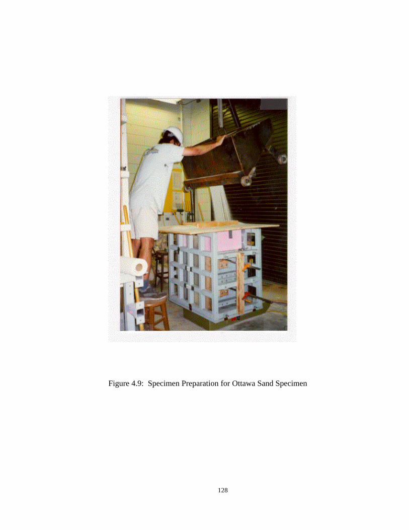
128

Figure 4.9: Specimen Preparation for Ottawa Sand Specimen

129

Figure 4.10: Specimen Preparation for Road Base Soil Specimen

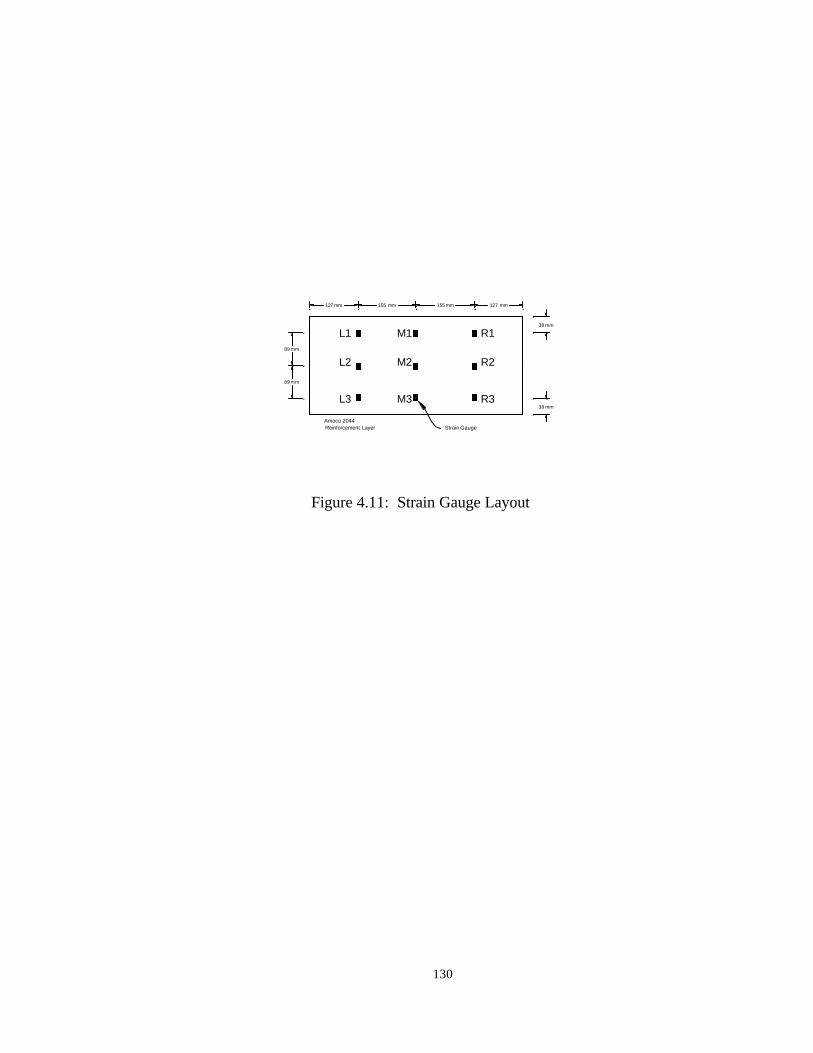
130

Figure 4.11: Strain Gauge Layout

155 mm

89 mm

Amoco 2044 Reinforcement Layer

89 mm

M3L3

L2 M2

127 mm 155 mm

L1 M1

R3

R2

38 mm

127 mm

R138 mm

Strain Gauge

131

Figure 4.12: Strain Gauge Calibration with LE Test

132

Figure 4.13: Calibration Curve for Strain Gauges

y = 3.0841xR2 = 0.975

0

0.5

1

1.5

2

2.5

3

3.5

4

0 0.2 0.4 0.6 0.8 1 1.2

Average Strain from LVDT (%)

Mea

sure

d Vo

ltage

from

Str

ain

Gau

ge (V

olt)

133

4.3 Test Programs Test programs for the SGP tests are presented in Table 4.1 for the Ottawa sand and Table 4.2 for the Road Base soil. The test program was divided into two groups: monotonic- loading (M) tests and unloading-reloading (UR) tests. The monotonic tests were conducted in a strain-controlled mode at a constant strain rate of 0.5% per minute. The unloading-reloading (UR) tests were conducted in a stress-controlled mode with various loading sequences at a constant loading rate of 10 kPa per minute, followed by a strain-controlled mode at a constant strain rate of 0.5% per minute up to failure. The monotonic loading SGP test program was designed for the following purposes: 1. To examine the reinforcing effects during the monotonic loading

Tests P-M-S vs. P-M-(S+3301) and P-M-(S+2044); and Tests P-M-RB vs. P-M-(RB+2044).

2. To provide a reference for an assessment of the effects of preloading on the GRS mass.

The unloading-reloading SGP test program was designed for the following purposes: 1. To examine the effects of preloading on the GRS mass

Tests P-M-(S+2044) vs. P-UR-(S+2044)-1; and Tests P-M-(RB+2044) vs. P-UR-(RB+2044).

2. To examine the effects of different types of unloading-reloading cycles For RL-Z path vs. RL-PS path: Tests P-UR-(S+2044)-1 vs. P-UR-(S+2044)-3; and Tests P-UR-(RB+2044). For multiple unloading-reloading cycles at the working load level: Tests P-UR-(S+2044)-2 and P-UR-(RB+2044). The working load level is defined as the vertical load with a magnitude less than the PLL.

3. To examine the effects of preloading magnitude on the GRS mass Tests P-UR-(S+2044)-1 vs. P-UR-(S+2044)-2; and Test P-UR-(RB+2044)).

4. To examine the reinforcing effects during the unloading-reloading cycles Tests P-UR-S vs. P-UR-(S+2044)-1; and Tests P-UR-RB vs. P-UR-(RB+2044).

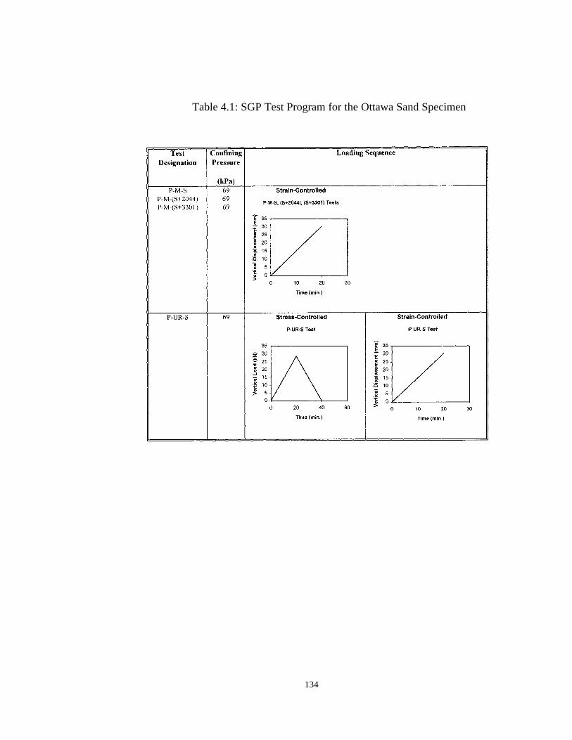
134

Table 4.1: SGP Test Program for the Ottawa Sand Specimen

135

Table 4.1: SGP Test Program for the Ottawa Sand Specimen (Continued)

136

Table 4.2: SGP Test Program for the Road Base Soil Specimen

137

5. Behavior of GRS Mass Subject to Monotonic Loading and Unloading-Reloading Cycles and Finite Element Analysis

This chapter presents experimental results and finite element analyses of the modified SGP tests conducted in this study. A total of 11 SGP tests were conducted to investigate the behavior of GRS masses subject to monotonic loading and unloading-reloading cycles. The finite element analyses were conducted to determine the stress distribution of a GRS mass in the SGP test.

To present the SGP test results, the following terms and symbols were used: Vertical load = applied vertical load from the MTS-810 loading

system Vertical displacement = vertical displacement of the rigid loading plate Horizontal displacement = sum of the horizontal displacements on two sides

of the specimen at a particular height Average horizontal displacement = average horizontal displacement of three measured

locations along the specimen height Sand mass = Ottawa sand specimen without reinforcement Road Base soil mass = Road Base soil specimen without reinforcement GRS mass = soil specimen with reinforcement Preloading curve = load-displacement curve during preloading Unloading curve = load-displacement curve during unloading Reloading curve = load-displacement curve during reloading PL = preloading UL = unloading RL = reloading PLL = preloading load level ULL = unloading load level PSL = prestressed load level WLL = working load level 5.1 Monotonic-Loading SGP Test Results and Discussions The monotonic- loading SGP test results and discussions of the test results are presented in this section. The discussions are focused primarily on the comparison of the test results of the soil mass with and without reinforcement. Figure 5.1 shows plots of the vertical and horizontal (at mid-height) displacements versus the vertical load of the Road Base soil mass without reinforcement (Test P-M-RB) and with Amoco 2044 geotextile reinforcement (Test P-M-(RB+2044)). Figure 5.2 shows plots of the vertical and horizontal (at mid-height) displacements versus the vertical load of the Ottawa sand mass without reinforcement (Test P-M-S), with Typar 3301

138

geotextile reinforcement (Test P-M-(S+3301)), and with Amoco 2044 geotextile reinforcement (Test P-M-(S+2044)).

The test results show that, at the same vertical load, the GRS mass experienced less vertical and horizontal displacements than the soil mass. At 10-kN vertical load, the Road Base soil mass and the corresponding GRS mass had vertical displacements of 6.36 mm and 4.58 mm, respectively, and horizontal displacements of 2.11 mm and 0.69 mm, respectively. At 35-kN vertical load, the Ottawa sand mass had a vertical displacement of 9.90 mm; with Typar 3301 reinforcement the vertical displacement was 7.59 mm, and with Amoco 2044 reinforcement it was 7.63 mm. The horizontal displacement of Test P-M-S was not available due to measurement errors.

The GRS masses also had higher failure loads. The Road Base soil mass had a failure load of 11.3 kN, whereas the corresponding GRS mass had a failure load of 16.9 kN. The Sand mass had a failure load of 37.4 kN; with Typar 3301 reinforcement the failure load was 44.7 kN, and with Amoco 2044 reinforcement it was 53.0 kN. These results demonstrate the reinforcing effects resulting from reinforcement layers in the GRS mass. It is seen in Figure 5.2 that the initial vertical stiffness of the GRS mass with Typar 3301 was somewhat smaller than that of the Sand mass. This behavior, referred to as loss of compressive stiffness has been reported in triaxial and plane strain tests of GRS specimens (see, e.g., Broms, 1977; Holtz et al., 1982). It was explained by Wu (1989) and described in Section 2.4.1. At small displacements, the soil and GRS masses showed almost identical deformation responses (see Figures 5.1 and 5.2). The reinforcement prohibited the specimen deformation after some vertical and horizontal displacements had occurred. This behavior can be explained by the load transfer mechanism of the GRS mass. Under a vertical load, the GRS mass deformed in both vertical and horizontal directions. The horizontal deformation induced the restraining effect from the reinforcement through interface friction. However, in a range when deformation was small, the magnitude of the horizontal deformation may not be sufficient to mobilize the restraining effect. This results in the same deformation response of the soil and GRS masses at small strains. In the Road Base soil mass with and without reinforcement, the required vertical and horizontal displacements were 2.0 mm and 0.5 mm, respectively. The magnitude of the required deformation depends on the stiffness of the soil, reinforcement, and interface.

The horizontal displacements at Points B, M, and T (i.e., ¼, ½, and ¾ of the specimen height, see Figure 4.3) of the Road Base soil and GRS masses at 4-kN, 8-kN, and 11-kN vertical loads were shown in Figure 5.3. Figure 5.3 clearly illustrates the reinforcing effects in reducing the horizontal deformation. The Road Base soil mass showed the largest horizontal movement at Point B and the least movement at Point T. For the GRS mass, Points T and B showed comparable

139

horizontal displacements. The smallest horizontal displacement occurred at Point M. At the vertical load of 11 kN, the horizontal displacements at Points T, M, and B were, respectively, 2.27 mm, 4.04 mm, and 6.63 mm in the Road Base soil mass. The corresponding displacements were 1.67 mm, 0.81 mm, and 1.44 mm in the GRS mass. Two types of failure modes, a diagonal shear failure and a wedge-type shear failure, were observed in these SGP tests. Figure 5.4 shows sketches of both failure modes. Figures 5.5 and 5.6 depict the specimens after failure for Tests P-M-RB and P-UR-(RB+2044), which show, respectively, the diagonal shear failure and wedge-type shear failure modes.

The first failure mode involved a single shear plane across a diagonal direction of the specimen. This failure mode occurred in the Sand and Road Base soil masses and the Sand mass with a weak reinforcement (Typar 3301). As shown in Figures 5.5, the shear band was evident along the diagonal direction from the top to the bottom of the specimen. In the test with Typar 3301 reinforcement, the middle reinforcement layer ruptured along the center line. The rupture location was approximately the intersection of the shear plane and the middle reinforcement layer. The reinforcement delayed a full development of the diagonal shear plane and, hence, increased the load carrying capacity of the soil mass.

The second failure mode was a wedge-type shear failure (see Figure 5.6). It occurred in the GRS mass with a strong reinforcement (Amoco 2044). The specimen experienced the wedge-type shear failure in the lower part of the specimen without reinforcement rupture. It appears that the strong reinforcement had altered the failure mode from the diagonal shear failure mode to the wedge-type shear failure mode.

140

Figure 5.1: Vertical Load Versus Displacement Relationships of Tests P-M-RB and P-M-(RB+2044)

0

2

4

6

8

10

12

14

16

18

20

0 5 10 15 20 25 30 35 40

Vertical Displacement (mm)

Vert

ical

Loa

d (k

N)

P-M-RBP-M-(RB+2044)

0

2

4

6

8

10

12

14

16

18

20

0 2 4 6 8 10 12

Horizontal Displacement at Pt. M (mm)

Vert

ical

Loa

d (k

N)

P-M-RBP-M-(RB+2044)

141

Figure 5.2: Vertical Load Versus Displacement Relationships of Tests P-M-S, P-M-(S+3301), and P-M-(S+2044)

0

10

20

30

40

50

60

0 5 10 15 20 25 30 35 40

Vertical Displacement (mm)

Vert

ical

Loa

d (k

N)

P-M-SP-M-(S+3301)P-M-(S+2044)

0

10

20

30

40

50

60

0 2 4 6 8 10 12

Horizontal Displacement at Pt. M (mm)

Vert

ical

Loa

d (k

N)

P-M-(S+3301)P-M-(S+2044)

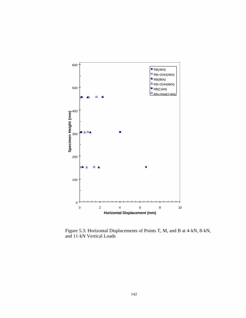
142

Figure 5.3: Horizontal Displacements of Points T, M, and B at 4-kN, 8-kN, and 11-kN Vertical Loads

0

100

200

300

400

500

600

0 2 4 6 8 10Horizontal Displacement (mm)

Spec

imen

Hei

ght (

mm

)RB(4kN)RB+2044(4kN)RB(8kN)RB+2044(8kN)RB(11kN)RB+2044(11kN)

143

Figure 5.4: Two Failure Modes in SGP Tests

Diagonal shear failure

Soil mass

Wedge-typeshear failureGRS mass with strong reinforcement layers (e.g., Amoco 2044)

GRS mass with weak reinforcement layers (e.g.,Typar 3301)

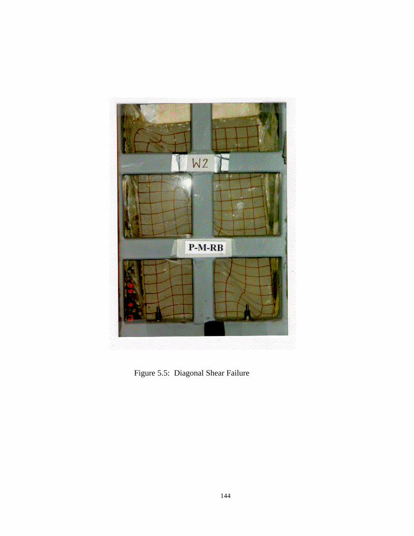
144

Figure 5.5: Diagonal Shear Failure

145

Figure 5.6: Wedge-Type Shear Failure

146

5.2 Unloading-Reloading SGP Test Results and Discussions A series of plots of the vertical load versus displacement relationships for unloading-reloading SGP tests is shown in Figures 5.7 to 5.10 for the Sand and GRS masses and in Figures 5.11 and 5.12 for the Road Base soil and GRS masses. A detailed description of the loading sequences for the tests was given in Section 4.3. The full-scale load test results of the FHWA pier were presented in Figure 5.13 and compared with the SGP test results. The load test results of the FHWA pier were adapted from Adams (1997).

From the results of the unloading-reloading SGP tests and the load test of the FHWA pier, the following observations were made.

1. Displacements During the PL Path: Both the SGP test and the FHWA pier showed vertical settlements and horizontal expansions under the PL path. After the SGP test specimen was unloaded and reloaded, the load-displacement curve resumed the preloading curve after the vertical load exceeded the PLL (see Figures 5.7 to 5.12). The preloading curve in the unloading-reloading SGP test was similar to the load-displacement curve of the corresponding monotonic SGP test (Test P-M-S vs. Test P-UR-S, Test P-M-RB vs. Test P-UR-RB, Test P-M-(S+2044) vs. Tests P-UR-(S+2044)-1 and P-UR-(S+2044)-2, and Test P-M-(RB+2044) vs. Test P-UR-(RB+2044)). This behavior indicates that the preloading curve of the soil mass with and without reinforcement is almost unaffected by the previous unloading-reloading cycles that occur at lower stress level. In the FHWA pier, the vertical loads in the RL path did not exceed the PLL.

2. Displacements During the Initial Stage of the UL Path: During the initial stage of the unloading path (from PLL to 0.95⋅PLL in the Sand and GRS masses and from PLL to 0.9⋅PLL in the Road Base soil and GRS masses), the SGP test specimen continued to deform in the same manners as in the PL path (i.e., settled and horizontally expanded). This behavior indicates potential creep deformation of the specimen at the PLL. This behavior was more pronounced in the Road Base soil than the Sand, in the horizontal movement than the vertical movement, and at the higher PLL than the lower PLL. The similar deformation behavior was also observed during the initial unloading path in the CTC tests of the soils (see Section 3.4.5.1). There was no data available during the unloading path of the FHWA pier.

3. Displacements During the UL Path After Passing the Initial Stage: For the rest of the unloading path, the SGP test specimen and the FHWA pier rebounded toward returning to the original shape. Both the SGP test specimen and the FHWA pier expanded vertically and contracted horizontally. After unloading, the irrecoverable deformation occurred in both vertical and horizontal directions of the SGP test specimen and the FHWA pier.

4. Unloading Stiffness: The unloading stiffness was approximately constant until the vertical load was reduced to a certain load level, referred to as the unloading threshold load. Below the unloading threshold load, the unloading stiffness became

147

much smaller. In other words, the specimen experienced a significant increase in the swelling rate at the unloading threshold load.

The unloading threshold load can be determined as the point of intersection of two straight lines tangent to the upper and lower portions of the unloading curve. The test data showed that the unloading threshold load was nearly the same for the soil mass with or without reinforcement, as shown in Figures 5.7, 5.8, 5.11, and 5.12. The unloading threshold load was found to be 0.15⋅PLL for the Sand and GRS masses (see Figures 5.7 and 5.8) and 0.25⋅PLL for the Road Base soil and GRS masses (see Figures 5.11 to 5.12). It was observed that reduction of the unloading stiffness below the unloading threshold load was more pronounced in the Sand specimens than the Road Base soil specimens. It is to be noted that in the UL-PS paths, the soil and GRS masses did not show this deformation behavior during unloading. This is because the ULL of the UL-PS paths (i.e., ULL=PSL) was higher than the unloading threshold load. The unloading threshold load will be used as a criterion for differentiating between the reloading stiffness of the RL-PS path and the RL-Z path in the simplified preloading-reloading (SPR) model. The SPR model will be described in detail in Chapter 6.

5. Displacements During the RL Path of the Sand : During the RL path, the Sand and GRS masses showed vertical settlements and horizontal expansions similar to the deformation behavior during the PL path. The vertical reloading curve of the RL-Z path of the Sand and GRS masses showed small stiffness at the initial stage. The vertical reloading stiffness gradually increased with the reloading magnitude until a vertical load was 0.15⋅PLL (see Figures 5.7, 5.8, and 5.9). After 0.15⋅PLL vertical load, the test specimens behaved approximately linearly. When the reloading magnitude approached the PLL, the reloading stiffness started to decrease. This behavior is known as the Bauschinger effect, as described in Section 3.4.5.

The small vertical stiffness during the initial stage of the RL-Z path is referred to as the reduced reloading stiffness. From Figures 5.7, 5.8, and 5.9, it appears that the reduced reloading stiffness behavior started from the ULL (i.e., the zero- load level for the RL-Z path), and ended at a reloading magnitude approximately equal to the unloading threshold load. The horizontal deformation during the RL-Z path did not show the reduced reloading stiffness. The FHWA pier (see Figure 5.13) and the Road Base soil and GRS masses (see Figures 5.11 and 5.12) also showed the reduced reloading stiffness in a vertical direction but not as obviously as in the Sand specimen. For the specimen under the RL-PS path, the reduced reloading stiffness did not occur in either vertical or horizontal directions. This interesting deformation characteristic is explained in the following paragraphs on the basis of the concept of principal stress rotation.

It is a well-known fact that principal stress rotation affects deformation response of many soils. This phenomenon is known as stress-induced stiffness anisotropy (e.g., Arthur et al., 1977; Mould et al., 1982). Mould (1983) conducted a

148

series of tests on Leighton Buzzard sand with a multiaxial cubical device. The specimen was first loaded and unloaded along the same stress path. In the subsequent reloading, the major principal stress was rotated 90° relative to its initial direction. It was found that the reloading response of the soil was softer than the virgin loading response. Also, the stiffness of the reloading curve decreased with increasing preloading level.

The vertical displacement of the SGP test specimen was a response of a particular boundary problem. The reduced reloading stiffness was most likely due to the reduction of vertical stiffness of a portion of soil in the specimen resulting from rotations of the principal stress directions. The principal stress rotation in some part of the SGP test specimen is explained in the following paragraphs and shown in Figure 5.14.

It is assumed that directions of compressive major and minor principal stresses are parallel to the vertical and horizontal axes, respectively. At the initial stage, the initial vertical and horizontal stresses (Point A in Figure 5.14) are, respectively, major and minor principal stresses. Under a vertical load, the vertical and horizontal stresses increased from Point A to B. Upon unloading to a zero-load level, the vertical stress was reduced to the initial vertical stress (Point C). Note that there exists a residual or “locked- in” horizontal stress (see Figure 5.14). The sum of the residual and initial horizontal stresses in some particular area may be larger than the vertical stress and causes rotations of the principal stress. As a result, the vertical stiffness of such an area in a subsequent vertical reloading (Point C to D) was small initially. The vertical stiffness gradually increases with the reloading magnitude as the major principal stress rotates back to the vertical direction. The unloading threshold load may be considered as the dividing point along the unloading path (Point B to C). When the vertical load is reduced below the unloading threshold load, the horizontal stress in a portion of the specimen becomes the major principal stress and results in softening of the vertical unloading stiffness and reducing of the subsequent vertical reloading stiffness.

Figure 5.14 also shows the stress path for an RL-PS path. In the RL-PS path, the test specimen is unloaded from Point B′ to C′. During unloading, both the vertical and horizontal stresses decreased along the same stress path as in the unloading path of the RL-Z path. However, unlike the unloading path of the RL-Z path, the magnitude of the vertical stress from Point B′ to C′ remains larger than the horizontal stress. Therefore, from Point B′ to C′, there is no principal stress rotation from a vertical direction to a horizontal direction. As a result, the reduced reloading stiffness did not occur in the subsequent reloading path from Point C′ to D′ (i.e., RL-PS path).

It should be pointed out that the stress paths presented in Figure 5.14 were assumed and were not from actual measurement. The above explanation for the reduced reloading stiffness may be validated by conducting a numerical analysis of the unloading-reloading behavior. Such a numerical analysis requires a constitutive

149

soil model that can account for the stress- induced stiffness anisotropy such as the nesting surface models (see, e.g., Mroz, 1967; Provost, 1981).

6. Displacements During the RL Path for the Road Base Soil: After the UL path in which the rebounding deformation occurred, the SGP test specimen was subjected to the RL path. During the RL path, the Road Base soil and GRS masses showed vertical settlements and horizontal expansion similar to the deformation behavior during the PL path. The test specimens behaved approximately linearly during the RL path. When the reloading magnitude approached the PLL, the reloading stiffness started to decrease (i.e., the Bauschinger effect).

During the initial reloading path when the UL path took place at a high PLL (PLL = 11.5 kN), the rebounding deformation from the unloading path still persisted (see Figure 5.12). The GRS mass continued to rebound vertically and horizontally against the vertical reloading. This behavior was more significant in the horizontal direction than in the vertical direction.

The FHWA pier showed a similar rebounding behavior. As shown in Figure 5.13, the pier continued rebounding in both vertical and horizontal directions after unloading to zero. It is believed that the rebounding deformation caused a stiffer reloading response upon reloading until the reloading load was about 80 kPa. This is because the vertical reloading load was applied against the vertical rebounding deformation of the pier.

7. Displacement During the RL-Z Path Versus the RL-PS Path: The vertical reloading curve of the RL-PS path showed higher stiffness than that of the RL-Z path for the Road Base soil and GRS masses (see Figures 5.11 and 5.12) and the Sand and GRS masses (see Figures 5.8 and 5.10). This behavior also showed in the unloading-reloading CTC tests of soils and is illustrated in Figures 3.19 and 3.20 (Section 3.4.5). A comparison of the displacement during the RL-Z path versus the RL-PS path will be presented later in Section 5.3.1.

8. Reinforcement Strains During Unloading-Reloading Cycles: The strains in the middle reinforcement layer of Test P-UR-(RB+2044) were measured by strain gauges. Of a total of 9 strain gauges, only gauges R-2 and R-3 (see Figure 4.11 for gauge locations) operated properly. This may due to mechanical damage of the gauges during specimen preparation by compaction. The specimen was compacted by a standard 4- lb Proctor hammer with 25-mm-thick compaction lifts. It was learned afterwards that the thickness of the compaction lift should be at least 200 mm to minimize possible mechanical damage. The 200-mm thickness is based on the reinforcement spacing of the FHWA pier. A total of 84 strain gauges were mounted on the reinforcement layers of the FHWA pier by the same technique employed in this study. Most of the gauges survived during construction and subsequent loading tests. The measured strains correlated well with the measured lateral displacements (Adams, 1997).

150

Due to the limited number of workable strain gauges, the measured strains were interpreted qualitatively. Figure 5.15 shows the relationship of the measured tensile strains from gauge R-3 (see Figure 4.11 for location) versus the vertical load. Generally speaking, the load-strain curve was similar to the load-horizontal displacement curve shown in Figure 5.12. The strain increased with increasing vertical loads. The load-strain curve showed horizontal creep behavior in the initial stage of the unloading path, and the tensile strains reduced during unloading. In the initial stage of reloading, the strains continued to reduce. This behavior conforms to the load-horizontal displacement behavior that the specimen continued to contract in the initial stage of reloading.

The irrecoverable strain was evident during unloading. The irrecoverable tensile strain has important implications for a preloaded GRS mass. First, it confirms the ratcheting mechanism (Tatsuoka et al., 1997), as explained in Section 2.4, in a preloaded GRS mass. Second, it indicates that there exists a residual or “locked-in” horizontal compressive stress in the soil after unloading because of the residual tensile forces of the reinforcement.

9. Effects of PLL Magnitude on Displacements in the RL Paths : The reloading curves under different PLL magnitudes of the GRS mass with the Sand (Tests P-UR-(S+2044)-1 and P-UR-(S+2044)-2) were almost identical (see Figure 5.16). The PLL magnitude was 28 kN in the former and 43 kN in the latter. The same behavior is also shown in the Road Base soil with and without reinforcement in which several PLL magnitudes were employed for the RL-Z and RL-PS paths. This indicates that the PLL magnitude does not affect the reloading deformation of the GRS mass except during the initial stage of the RL-Z path for the GRS mass with the Road Base soil, which showed some rebounding deformation following a high PLL.

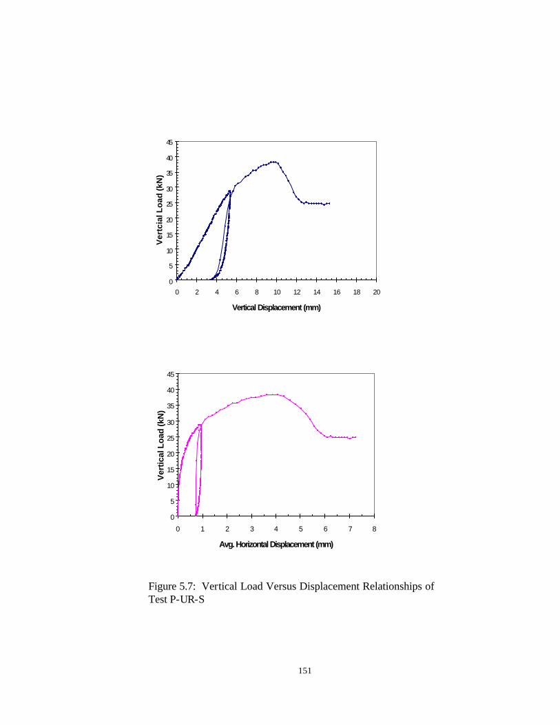
151

Figure 5.7: Vertical Load Versus Displacement Relationships of Test P-UR-S

0

5

10

15

20

25

30

35

40

45

0 1 2 3 4 5 6 7 8

Avg. Horizontal Displacement (mm)

Verti

cal L

oad

(kN

)

0

5

10

15

20

25

30

35

40

45

0 2 4 6 8 10 12 14 16 18 20

Vertical Displacement (mm)

Vert

cial

Loa

d (k

N)

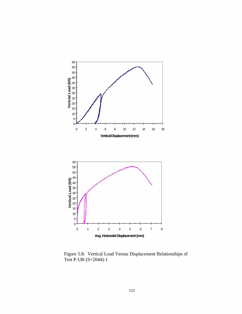
152

Figure 5.8: Vertical Load Versus Displacement Relationships of Test P-UR-(S+2044)-1

05

10

152025

303540

4550

5560

0 1 2 3 4 5 6 7 8

Avg. Horizontal Displacement (mm)

Verti

cal L

oad

(kN

)

05

10

152025

303540

4550

5560

0 2 4 6 8 10 12 14 16 18

Vertical Displacement (mm)

Vertc

ial L

oad

(kN

)

153

Figure 5.9: Vertical Load Versus Displacement Relationships of Test P-UR-(S+2044)-2

0

51015

2025

303540

455055

60

0 5 10 15 20

Vertical Displacement (mm)

Vertc

ial L

oad

(kN

)

05

10

152025

303540

4550

5560

0 2 4 6 8

Avg. Horizontal Displacement (mm)

Verti

cal L

oad

(kN

)

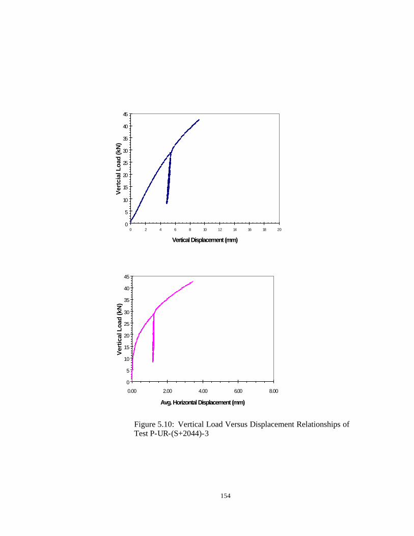
154

Figure 5.10: Vertical Load Versus Displacement Relationships of

Test P-UR-(S+2044)-3

0

5

10

15

20

25

30

35

40

45

0.00 2.00 4.00 6.00 8.00

Avg. Horizontal Displacement (mm)

Verti

cal L

oad

(kN

)

0

5

10

15

20

25

30

35

40

45

0 2 4 6 8 10 12 14 16 18 20

Vertical Displacement (mm)

Vertc

ial L

oad

(kN

)

155

Figure 5.11: Vertical Load Versus Displacement Relationships of Test P-UR-RB

0

2

4

6

8

10

12

14

0 2 4 6 8 10 12 14 16 18

Vertical Displacement (mm)

Vertc

ial L

oad

(kN

)

0

2

4

6

8

10

12

14

0 2 4 6 8 10

Avg. Horizontal Displacement (mm)

Verti

cal L

oad

(kN

)

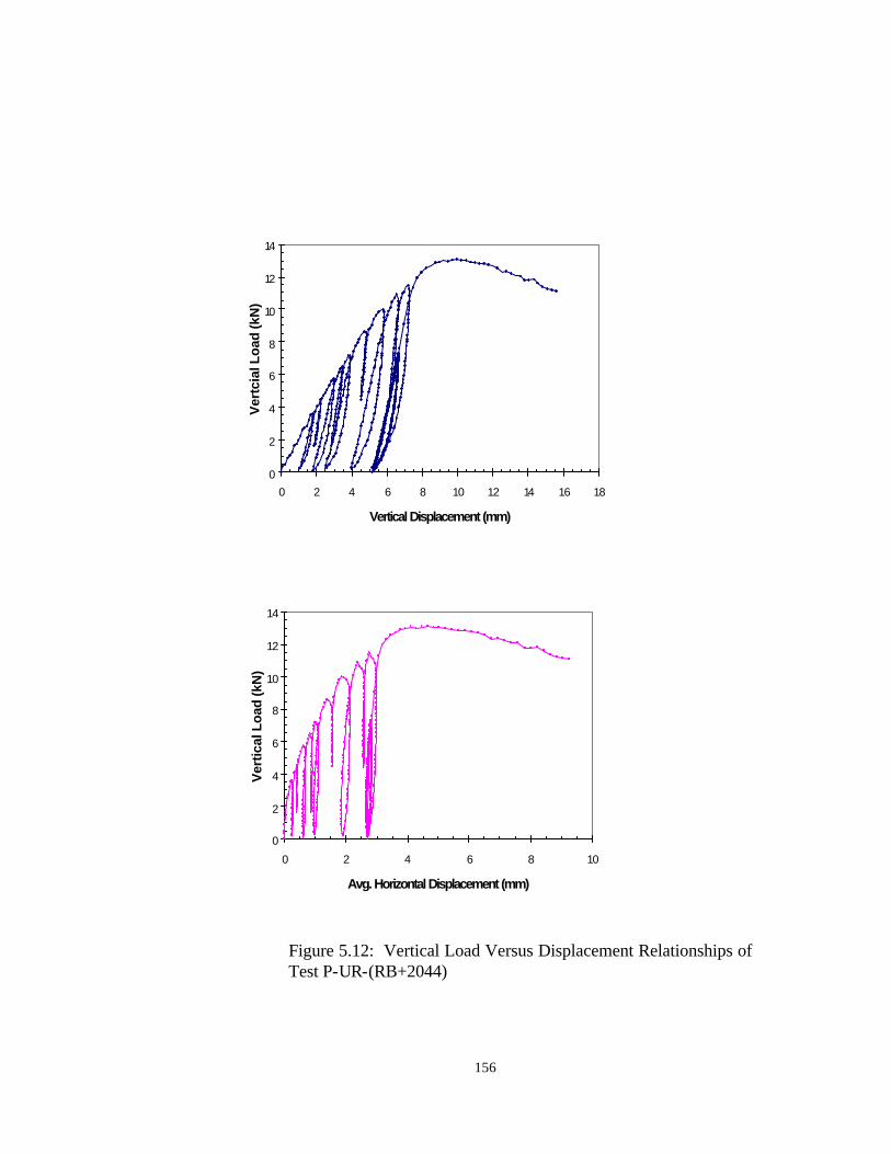
156

Figure 5.12: Vertical Load Versus Displacement Relationships of Test P-UR-(RB+2044)

0

2

4

6

8

10

12

14

0 2 4 6 8 10 12 14 16 18

Vertical Displacement (mm)

Vertc

ial L

oad

(kN

)

0

2

4

6

8

10

12

14

0 2 4 6 8 10

Avg. Horizontal Displacement (mm)

Verti

cal L

oad

(kN

)

157

Figure 5.13: Vertical Applied Pressure Versus Displacement Relationships of the FHWA Pier

0

100

200

300

400

500

600

700

800

900

1000

0 20 40 60 80 100

Displacement (mm)

Vert

ical

App

lied

Pres

sure

(kPa

)

VerticalHorizontal

158

Figure 5.14: Conceptual Stress Diagrams for the RL-Z and RL-PS Paths

Initial Vertical Stress

Time

C'

A, A'Initial HorizontalStress

RL-Z Path

A C

Vertical Stress

B

Residual HorizontalStress C

Horizontal Stress

Time

Vertical Stress

D'D

RL-PS Path

A'

C'

Vertical Stress

B'

D

D'B, B'

159

Figure 5.15: Vertical Load Versus Reinforcement Strain Relationship of Test

P-UR-(RB+2044), Gauge R-3 (see Figure 4.11 for gauge location)

0

2

4

6

8

10

12

14

0.00 0.10 0.20 0.30 0.40 0.50 0.60 0.70 0.80

Measured Strain (%)

Vert

ical

Loa

d (k

N)

160

10. Multiple Unloading-Reloading Cycles at a Working Load Level: Three tests were conducted in such a manner that the specimen was subjected to multiple loading-unloading cycles at a “working” load level. The specimen was subjected to five reloading-unloading cycles at 15 kN (0.35% of PLL) in Test P-UR-(S+2044)-2 (see Figure 5.9), at 3.6 kN (50% of PLL) in Test P-UR-RB (see Figure 5.11), and at 7.2 kN (60% of PLL) in Test P-UR-(RB+2044) (see Figure 5.12). From the figures, it is seen that the load-displacement curves under the multiple unloading-reloading cycles at working load levels approximately coincided with one another. This indicates that the deformation response of the soil and GRS masses is not influenced by multiple reloading-unloading cycles at working load levels. This behavior was also observed in the FHWA pier and the Black Hawk abutments (see Figures 7.1, 7.5, and 7.6 in Chapter 7). Adams (1997) and Wu et al. (1999) stated that the effects of preloading in reducing the deformation of the structure were minute in subsequent reloading cycles.

11. Hysteresis Loops: Hysteresis loops existed in all unloading-reloading cycles (see Figures 5.7 to 5.12). The hysteresis loop is an indication of energy dissipation during an unloading-reloading cyc le. The area of the hysteresis loop can be used to determine a damping ratio of a soil. A detailed analysis of the hysteresis loops may be carried out in future studies of the dynamic behavior of preloaded GRS masses. Only general observations of the hysteresis loop were made in this study. It is seen that the hysteresis loop area increased when the unloading-reloading cycle took place at the higher PLL. As shown in Figures 5.11 and 5.12, at the comparable PLL, the area of hysteresis loop was smaller for unloading-reloading cycles performed at a prestressed load level (i.e., UL-PS and RL-PS paths) than at zero- load level (i.e., UL-Z and RL-Z paths).

5.3 Effects of Preloading on Deformation and Strength of GRS Mass Effects of preloading on deformation and strength of GRS masses were assessed in the following sections. 5.3.1 Effects of Preloading on Deformation

To assess the effects of preloading on deformation, the displacements of monotonic loading SGP tests were compared with reloading displacements of the unloading-reloading SGP tests. In comparing the displacements, the displacements of the monotonic- loading and unloading-reloading tests were presented in the same plot. In the plot, the reloading displacement was referenced to the deformed shape of the test specimen after the end of the unloading path. The reloading displacement was considered as the displacement of a preloaded specimen, whereas the displacement under monotonic loading was considered as the displacement of a virgin specimen.

The displacements under monotonic loading and reloading paths of the GRS masses with the Sand are presented in Figure 5.16. Figure 5.16 shows the vertical

161

and average horizontal displacements versus vertical load relationships for Test P-M-(S+2044) (for monotonic loading), Tests P-UR-(S+2044)-1 and 2 (for the RL-Z path), and Test P-UR-(S+2044)-3 (for the RL-PS path). The displacements of the monotonic loading were compared with those of the RL-Z and RL-PS paths.

It can be seen that, at the same vertical load, the preloaded specimen experienced less vertical and horizontal displacements than the virgin specimen. The RL-PS path showed higher stiffness than the RL-Z path in the vertical direction, but the stiffness was similar in the horizontal direction for vertical loads less than 20 kN. At a vertical load of 20 kN, the vertical and horizontal displacements of the virgin specimen were 4.05 mm and 0.26 mm, respectively. At the same vertical load, the vertical and horizontal displacements of the preloaded specimen were 1.23 mm and 0.02 mm, respectively, in the RL-Z path and 0.56 and 0.05, respectively, in the RL-PS path. A similar reduction of the displacements upon preloading was observed in the GRS masses with the Road Base soil as shown in Figures 5.33 and 5.34. Figure 5.17 shows the vertical and average horizontal displacements versus vertical load relationships for Test P-M-(RB+2044) (for monotonic loading) and Test P-UR-(RB+2044) (for the RL-Z and RL-PS paths). The RL-PS paths include two tests with different prestressed load levels (PSL). The value of PSL was 1.5 kN for the RL-PS1 path and 4.5 kN for the RL-PS2 path. The displacements of the monotonic loading were compared with those of the RL-Z, RL-PS1, and RL-PS2 paths.

The preloaded specimen showed stiffer deformation responses in both vertical and horizontal directions. At the same vertical load, the RL-PS2 path yielded the least value of the vertical displacement, followed by the RL-PS1 path, then the RL-Z path. This indicates that the vertical stiffness of the preloaded GRS mass increases with the prestressed load level (PSL) or the unloading load level (ULL). The horizontal displacements of all reloading paths were comparable. At a vertical load of 4 kN, the vertical and horizontal displacements of the virgin specimen were 1.79 mm and 0.18 mm, respectively. At the same vertical load, the corresponding displacements of the preloaded specimen were 0.82 mm and –0.02 mm in the RL-Z path, 0.56 mm and 0.03 mm in the RL-PS1 path, and 0.33 mm and 0.01 mm in the RL-PS2 path.

Effects of reinforcement (i.e., the reinforcing effect) during the reloading paths were also examined. A series of plots comparing the reloading displacements of the soil and GRS masses was shown in Figures 5.18 to 5.20. Figure 5.18 compares the displacements under the RL-Z path of the Sand mass with and without reinforcement. Figure 5.19 compares the displacements under the RL-Z path of the Road Base soil mass with and without reinforcement. Figure 5.20 compares the displacements under the RL-PS path of the Road Base soil mass with and without reinforcement. It can be seen that the soil mass with and without reinforcement showed nearly identical vertical and horizontal reloading curves in some cases. In

162

other cases, the soil mass with reinforcement showed slightly stiffer response. This indicates that the effect of reinforcement is insignificant during the reloading path.

5.3.2 Effects of Preloading on Strength Table 5.1 presents the peak vertical loads (i.e., the failure load) of the SGP tests conducted in this study. The peak loads of the preloaded specimens were slightly higher than those of the corresponding virgin specimens. The differences were in the range of 5% except for the Road Base soil specimen with reinforcement. The preloaded Road Base soil specimen with Amoco 2044 showed about 20% lower peak load than that of the corresponding virgin specimen. This may be because of the slight differences in the degree of compaction and water content.

The failure mode of the preloaded and virgin specimens was also similar. Tests P-UR-S and P-UR-RB showed a diagonal shear failure (see Section 5.1 for definition), whereas Tests P-UR-(S+2044)-1,2 and P-UR-(RB+2044) showed the wedge-type shear failure (see Section 5.1 fo r definition). Note that the reloading to failure load of Test P-UR-(S+2044)-3 was not available due to measurement errors.

163

Figure 5.16: Vertical Load Versus Displacements of Virgin Specimen from Test P-M-(S+2044) and Preloaded Specimens from Tests P-UR-(S+2044)-1,2,3

0

5

10

15

20

25

30

35

40

45

50

0 2 4 6 8 10 12

Vertical Displacement (mm)

Vert

ical

Loa

d (k

N)

P-M-(S+2044)P-UR-(S+2044)-1P-UR-(S+2044)-2P-UR-(S+2044)-3

0

5

10

15

20

25

30

35

40

45

50

0 0.5 1 1.5 2 2.5 3 3.5

Avg. Horizontal Displacement (mm)

Vert

ical

Loa

d (k

N)

P-M-(S+2044)P-UR-(S+2044)-1P-UR-(S+2044)-2P-UR-(S+2044)-3

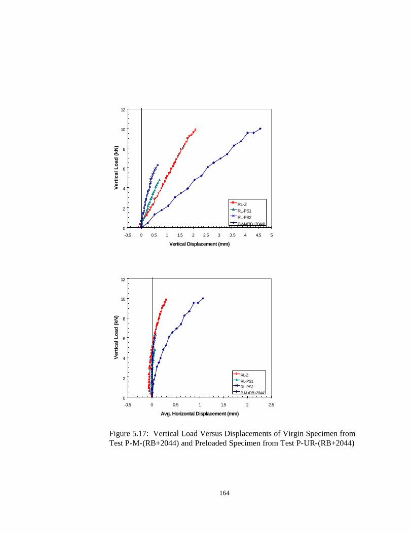
164

Figure 5.17: Vertical Load Versus Displacements of Virgin Specimen from Test P-M-(RB+2044) and Preloaded Specimen from Test P-UR-(RB+2044)

0

2

4

6

8

10

12

-0.5 0 0.5 1 1.5 2 2.5 3 3.5 4 4.5 5

Vertical Displacement (mm)

Vert

ical

Loa

d (k

N)

RL-ZRL-PS1RL-PS2P-M-(RB+2044)

0

2

4

6

8

10

12

-0.5 0 0.5 1 1.5 2 2.5

Avg. Horizontal Displacement (mm)

Vert

ical

Loa

d (k

N)

RL-ZRL-PS1RL-PS2P-M-(RB+2044)

165

Figure 5.18: Vertical Load Versus Reloading Displacement Relationships (RL-Z path) of Tests P-UR-S and P-UR-(S+2044)-1

0

5

10

15

20

25

30

35

0 0.5 1 1.5 2 2.5

Vertical Displacement (mm)

Vert

ical

Loa

d (k

N)

P-UR-SP-UR-(S+2044)-1

0

5

10

15

20

25

30

35

-0.05 0 0.05 0.1 0.15 0.2 0.25

Avg. Horizontal Displacement (mm)

Vert

ical

Loa

d (k

N)

P-UR-SP-UR-(S+2044)-1

166

Figure 5.19: Vertical Load Versus Reloading Displacement Relationships (RL-Z path) of Tests P-UR-RB and P-UR-(RB+2044)

0

1

2

3

4

5

6

7

8

-0.05 0 0.05 0.1 0.15 0.2

Avg. Horizontal Displacement (mm)

Vert

ical

Loa

d (k

N)

P-UR-RBP-UR-(RB+2044)

0

1

2

3

4

5

6

7

8

0 0.5 1 1.5 2 2.5 3

Vertical Displacement (mm)

Vert

ical

Loa

d (k

N)

P-UR-RBP-UR-(RB+2044)

167

Figure 5.20: Vertical Load Versus Reloading Displacement Relationships (RL-PS path) of Tests P-UR-RB and P-UR-(RB+2044)

0

1

2

3

4

5

6

7

8

0 0.5 1 1.5 2 2.5

Vertical Displacement (mm)

Vert

ical

Loa

d (k

N)

P-UR-RBP-UR-(RB+2044)

0

1

2

3

4

5

6

7

8

-0.05 0 0.05 0.1 0.15 0.2

Avg. Horizontal Displacement (mm)

Vert

ical

Loa

d (k

N)

P-UR-RBP-UR-(RB+2044)

168

Table 5.1: Summary of Failure Loads of the SGP Tests

Test Soil Reinforcement Peak Vertical Load (kN)

P-M-S S - 37.4

P-UR-S S - 38.2

P-M-RB RB - 11.3

P-UR-RB RB - 11.8

P-M-(S+3301) S Typar 3301 44.7

P-M-(S+2044) S Amoco 2044 53

P-UR-(S+2044)-1 S Amoco 2044 55.2

P-UR-(S+2044)-2 S Amoco 2044 56

P-UR-(S+2044)-3 S Amoco 2044 N/A

P-M-(RB+2044) RB Amoco 2044 16.9

P-UR-(RB+2044) RB Amoco 2044 13.1

169

5.4 Finite Element Analysis of the SGP Test Finite element analyses were conducted to examine the stress distribution of a GRS mass in the SGP test subject to monotonic loading. The analysis results and the SGP test results provided a basis for developing the simplified preloading-reloading (SPR) model. A finite element analysis for the unloading-reloading SGP tests was not conducted because the results of the SGP tests and the finite element analyses of the monotonic- loading SGP tests were judged to be sufficient for developing the SPR model.

The program SSCOMPPC (a finite element analysis program for evaluation of soil-structure interaction and compaction Effects) was used. The SSCOMPPC has been used with success to predict reinforced-soil wall behavior (Collin, 1986; Adib, 1988; Jaber, 1989). The following subsection briefly describes the program, the material and interface behavior models, and determination of the model parameters. A detailed description of the program can be found in the SSCOMPPC manual by Boulanger et al.(1991).

5.4.1 Program Description

The program SSCOMPPC is a general purpose, plane strain, soil-structure interaction finite element program for static analysis of geotechnical problems. The program SSCOMPPC is the PC version of the program SSCOMP (Seed and Duncan, 1984). The program calculates stresses, strains, and displacements in soil elements, and internal forces and displacements in structural elements by simulating the actual sequence of construction operations in a number of steps. The nonlinear and stress-dependent stress-strain properties of the soils are approximated by varying the values of modulus and Poisson’s ratio in accordance with calculated stresses by using the modified hyperbolic model (Duncan et al., 1980). The structural materials are assumed to behave linearly.

An increment of an analysis may be placement of a layer of fill, compaction of a layer of fill, or application of loads. For an increment of analysis, two iterations are performed. The first iteration uses soil modulus and Poisson’s ratio values based on the stresses in each soil element at the beginning of the increment. The second iteration uses adjusted soil modulus and Poisson’s ratio values based on the average stresses during the increment.

5.4.2 Material and Interface Behavior Models 5.4.2.1 Soil Behavior Model

The hyperbolic stress-strain model for soils was first proposed by Kondner (1963) and modified by Duncan and Chang (1970) and Duncan et al. (1980). It has been widely used in finite element analysis of different earth structures (Duncan, 1994). Ko and Sture (1981) pointed out some limitations inherent in the model. The

170

model is based on the generalized Hooke’s law for isotropic material. As a result, it is not capable of modeling shear dilatancy (i.e., volume change during shear) of soils. If the loading path deviates significantly from that of triaxial compression, the strains predicted by the model may not be accurate. Another limitation is that the model does not realistically model at and after peak responses of soils (Duncan, 1994).

In spite of the aforementioned limitations, the model has several advantages that lead to its popularity in geotechnical engineering applications. First, the model parameters are easily understood and can be related to the deformation behavior of the soil. Second, only standard triaxial compression tests are needed for determination of the model parameters. Third, the large database of the model parameters is available in the literature for a wide variety of soil types under both drained and undrained conditions. Duncan (1994) suggested that the model is adequate under the following conditions: 1. The factor of safety against global stability is high enough. 2. If local failure occurs, it does not control behavior in any region where accurate

results are needed. 3. The conditions analyzed are either fully drained (and analyzed in terms of

effective stress) or completely undrained (and analyzed in terms of total stress). The hyperbolic stress-strain model appears to be adequate for the

determination of the pre-peak stress distributions of the GRS mass in the monotonic-loading SGP test. The finite element analyses were only conducted on the Road Base soil mass with and without reinforcement because of the limitation of the soil model to simulate the shear dilatancy behavior of the medium-dense Ottawa sand. The nonlinear soil behavior model employed in the program SSCOMPPC is the modified hyperbolic stress-strain model (Duncan et al., 1980; Seed and Duncan, 1984). The hyperbolic soil model parameters and the recommended methods for obtaining the parameters are presented in detail in Duncan et al. (1980). A brief description of the hyperbolic model parameters and parameter determination is presented below.

The hyperbolic soil model is a nonlinear (hyperbolic) incremental stress-strain and bulk modulus model. The model assumes that stress-strain curves for soils can be approximated as hyperbolas.

The soil material is considered as an isotropic elastic material. The nonlinear stress-strain relation is represented by the following hyperbolic relationship (see Figure 5.21):

ultiE )(1

31

311

1

σσε

εσσ

−+

=− [5.1]

where σ1-σ3 = deviator stress Ei = tangent Young’s modulus at the origin (σ1-σ3 = 0)

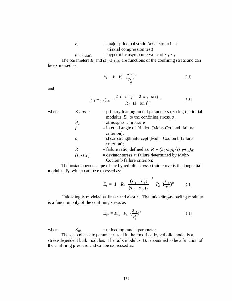
171

ε1 = major principal strain (axial strain in a triaxial compression test) (σ1-σ3)ult = hyperbolic asymptotic value of σ1-σ3

The parameters Ei and (σ1-σ3)ult are functions of the confining stress and can be expressed as:

n

aai P

PKE )( 3σ⋅⋅= [5.2]

and

)sin1(sin2cos2

)( 331 φ

φσφσσ

−⋅⋅⋅+⋅⋅

=−f

ult Rc

[5.3]

where K and n = primary loading model parameters relating the initial modulus, Ei, to the confining stress, σ3 Pa = atmospheric pressure

φ = internal angle of friction (Mohr-Coulomb failure criterion); c = shear strength intercept (Mohr-Coulomb failure

criterion); Rf = failure ratio, defined as: Rf = (σ1-σ3)f / (σ1-σ3)ult (σ1-σ3)f = deviator stress at failure determined by Mohr-

Coulomb failure criterion; The instantaneous slope of the hyperbolic stress-strain curve is the tangential modulus, Et, which can be expressed as:

n

aa

fft P

PRE )()()(

1 3

2

31

31 σσσσσ

⋅⋅

−−

⋅−= [5.4]

Unloading is modeled as linear and elastic. The unloading-reloading modulus is a function only of the confining stress as

n

aaurur P

PKE )( 3σ⋅⋅= [5.5]

where Kur = unloading model parameter The second elastic parameter used in the modified hyperbolic model is a stress-dependent bulk modulus. The bulk modulus, B, is assumed to be a function of the confining pressure and can be expressed as:

172

m

aab P

PKB )( 3σ⋅⋅= [5.6]

where Kb and m = Bulk modulus model parameters relating the bulk modulus, B, to the confining pressure, σ3

In a triaxial compression test, the volumetric strain can be related to the axial strain by the following equation:

av ενε ⋅−= )21( [5.7]

where ν = Poisson’s ratio The bulk modulus, B, can be expressed in terms of Et and ν as:

)21(3 ν−⋅= tE

B [5.8]

From Eq. 5.7 and 5.8, the following equation can be derived:

at

v BE

εε ∆⋅⋅

=∆3

[5.9]

At least three triaxial tests are needed to obtain the hyperbolic model parameters. The initial modulus, Ei, and the hyperbolic asymptotic value, (σ1-σ3)ult, from each triaxial test are first determined. The parameters Ei and (σ1-σ3)ult are determined by plotting ε1/(σ1-σ3) versus ε1. A linear regression can be used to obtain the best fitting straight line for each test.

The parameters K and n can be determined by plotting Ei/Pa versus σ3/Pa on a log- log scale. The best- fit straight line is drawn. The value of K is equal to the value of Ei/Pa where σ3/Pa is equal to unity of the best-fit line. The value of n is the slope of the line. The value of Kur is determined by assuming that the modulus exponent, n, for unloading-reloading was the same as that of primary loading. Eq. 5.5 can be written in the following form:

n

aa

urur

PP

EK

)( 3σ⋅

= [5.10]

173

The unloading-reloading modulus (Eur) can be determined from the deviator stress versus axial strain relationship of each triaxial test. The scattered values of Kur are averaged to give a representative value of Kur. Two steps are involved in determining the values of Kb and m. First, the bulk modulus (B) from each triaxial test was determined by the following equation:

v

Bεσσ

⋅−

=3

)( 31 [5.11]

The bulk modulus is determined at (σ1-σ3) = 0.7 (σ1-σ3)f and the corresponding value of εv. Second, the values of Kb and m are determined by plotting the values of B/Pa versus σ3/Pa on a log- log scale. The best-fit straight line is drawn. The value of Kb is equal to the value of B/Pa where σ3/Pa is equal to unity of the best-fit line. The value of m is the slope of the line. 5.4.2.2 Geosynthetic Behavior Model

The geosynthetic reinforcement was modeled by using linear-elastic one-dimensional bar elements that had axial stiffness but no flexural stiffness. The material properties can be obtained from the uniaxial load-extension test of the geosynthetic. Input for the bar element includes Young’s modulus and cross- sectional area.

The linear-elastic idealization is not realistic in some geosynthetics that show a significant nonlinear load-strain relationship under the anticipated stress range. Nonlinear relationships, as proposed by Ling and Tatsuoka (1992) or Chou and Wu (1993), may be used to model the non- linear behavior. The nonlinear model for a geosynthetic is typically established from a uniaxial load-extension test, either in a confined or unconfined condition, conducted at a constant strain rate. It must be noted that the load-strain relationship of some geosynthetics is strain-rate dependent. If the strainrate of the load-extension test for such a geosynthetic is significantly different from the GRS structure, a significant error may occur.

In this study, the reinforcement strains in the SGP test were expected to be relatively small (typically less than 1%). This was later confirmed by the measured strains of Test P-UR-(RB+2044) presented in Section 5.2. The load-extension test results obtained under stress- and strain-controlled modes showed that the load-strain relationship of Amoco 2044 reinforcement was approximately linear for strains less than 1%, and the behavior was strain-rate independent.

5.4.2.3 Soil-Geosynthetic Interface Model

The soil-geosynthetic interface is modeled by an assembly of nonlinear hyperbolic interface elements with normal and tangential springs (i.e., the method of stiffness). The interface element based on the method of stiffness has been widely used in the finite element analysis of soil-structure interaction problems. It was first

174

introduced by Goodman et al. (1968) for finite element analysis of jointed rock masses. The interface elements in the program SSCOMPPC are based on a nonlinear interface element that was developed by Clough and Duncan (1969).

The interface model consists of two parallel nodal links, as shown in Figure 5.22. Each nodal link comprises a normal spring and a shear spring. The properties of the interface element consist of a normal stiffness (of the normal springs), Kn, and a tangent shear stiffness (of the shear springs), Kst. The normal stress, σn, and the shear stress, τ, acting on the element are related to the normal and shear stiffness by the following equations:

nnnK σ=∆⋅ [5.12]

τ=∆⋅ sstK [5.13]

in which ∆n is the average relative normal displacement across the element, and ∆s is the average relative shear displacement along the element. The linear elastic normal stiffness, Kn, controls the opening and the compressing of the interface element between two adjacent two-dimensional elements. The normal stiffness is specified by a dimensionless coefficient as:

w

nn

Kk

γ= [5.14]

in which Kn is the normal stiffness, kn is the input normal spring coefficient (dimensionless), and γw is the unit weight of water. For compressive loading, the overlapping (or penetration) of the two-dimensional elements can be minimized by using a large normal spring stiffness. The analysis is carried out by using a “fixed” condition initially (i.e., assuming a “large” kn value). In the case of tension, the normal spring stiffness is set to zero by SSCOMPPC. The shear behavior of the interface is modeled by a hyperbolic relationship between the shear stress and the relative shear displacement at the interface, as shown in Figure 5.22. The equations that describe the hyperbolic model for the shear behavior are as follows: (a) Primary Loading and Reloading:

2

tan1

⋅+

⋅−

⋅⋅=

δσ

τσγ

n

fn

a

nwsst c

RP

kK [5.15]

in which Kst is the tangent shear stiffness, ks is the input shear spring coefficient (dimensionless), n and Rf are experimentally determined constants, γw is the unit

175

weight of water, Pa is the atmospheric pressure, δ is the interface frictional angle, c is the interface cohesion, and σn and τ are the normal stress and shear stress acting on the interface, respectively. (b) Unloading:

n

a

nwurst P

kK

⋅⋅=

σγ [5.16]

in which kur is the input unloading shear spring coefficient (dimensionless). The values of ks, kur, n, and Rf for an interface can be determined from laboratory tests, such as direct shear tests or other appropriate tests. The tests should be conducted between the relevant materials for the range of stresses expected in the application.

Wu (1993) pointed out two problems associated with the interface models using the method of stiffness. The first problem relates to determination of the value of shear spring stiffness, Kst. The value of Kst is typically determined by laboratory interface shear tests such as direct shear tests or pullout tests. These laboratory shear tests are model tests. The results of the model tests depend on the geometric conditions of the tests (e.g., specimen size). Therefore, the value of Kst is a function of the specimen size, among other variables. This implies that correct values of Kst must be deduced from an interface shear test of which the specimen size is nearly equal to the length of the interface segment in the finite element discretization.

The second problem relates to numerical difficulties that may arise in this approach. To minimize penetration between contacting nodes, a large normal spring stiffness is used. If the value of the normal spring stiffness is too small, significant penetration will occur, which is kinemetically incorrect. On the other hand, if the value of the normal spring stiffness is too large, the truncation error may become too large and the resulting stresses can be in significant error.

In this study, the first problem addressed by Wu (1993) was alleviated by compromising the length of the interface elements in the finite element discretization with the size of the specimen in the direct shear tests. The uniform length of the interface elements in the finite element discretization was about 20% of the specimen width of the direct shear tests. To prevent penetration of the contacting nodes and avoid the truncation error, the value of normal spring stiffness recommended by the SSCOMPPC manual was used.

5.4.3 Determination of Model Parameters

The model parameters needed for the analysis were determined by the recommended procedures described in Section 5.2.2. Results of the conventional triaxial compression (CTC) tests, the in- isolation load extension (LE) tests, and the direct shear tests (DS) were used.

176

5.4.3.1 Soil Model Parameters The soil model parameters for the Road Base soil were first determined from three CTC tests by the recommended procedure by Duncan et al. (1980). They were then adjusted to fit the deformation responses of the Road Base soil mass in the SGP test. Table 5.2 shows the parameters of the hyperbolic stress-strain model for the Road Base soil. The hyperbolic model parameters shown in Table 5.1 were used to back-calculate the results of the CTC tests. The model-simulated results as compared with the CTC test results are shown in Figure 5.23. The agreement between the two is considered acceptable. 5.4.3.2 Geosynthetic Model Parameters

The secant slope at 1% was used to represent the axial stiffness of the geosynthetic. From the load-strain relationship of Amoco 2044 geosynthetic, the secant slope at 1% strain was determined to be equal to 1,000 kN/m. In the analysis, the values of Young’s modulus of 1,000 kN/m2 and cross-sectional area of 1 m2 /m were assigned. These values give an axial stiffness value of 1,000 kN/m.

5.4.3.3 Soil-Geosynthetic Interface Model Parameters

The hyperbolic interface model parameters for the soil were determined from three unloading-reloading DS tests by a method similar to that used for the hyperbolic soil parameters. Table 5.2 shows the parameters of the hyperbolic interface model for the Road Base soil with Amoco 2044 geosynthetic. The hyperbolic model parameters shown in Table 5.2 were used to back-calculate the results of the DS tests. The model-simulated results as compared with the direct shear test results are shown in Figure 5.24. It is seen that the agreement between the two is good. 5.4.4 Finite Element Modeling

The reinforced soil specimen in the SGP test was modeled as a plane-strain two-dimensional problem in the finite element analysis. Four types of elements were used in the analysis: 1. Soil Elements: The soil elements in the SSCOMPPC program are four-noded, isoparametric elements. 2. Bar Elements: The bar elements are two-noded elements with axial stiffness only. These elements were used to model the geosynthetic reinforcement layers. 3. Interface Elements: The interface elements are zero-thickness elements that consist of two pairs of normal and shear springs. These elements were used to model the soil-geosynthetic interfaces and the lubrication layers. For lubrication layers, the friction angle was assumed to be 1.5°. 4. Beam Elements: The beam elements are two-node elements with axial, bending, and shear stiffness. These elements were used to model the rigid loading plate.

177

Relatively large values were assigned to the material properties to simulate large rigidity of the loading plate.

Figure 5.25 shows the finite element discretizations for the analysis of the SGP test with and without reinforcement. Only one-half of the geometry was analyzed due to symmetry.

The finite element mesh of the soil mass consisted of 462 nodes, 400 soil elements, 10 beam elements for the loading plate, and 10 interface elements for the lubrication layer between the loading plate and the soil. The finite element mesh of the soil mass with reinforcement consisted of 506 nodes, 400 soil elements, 10 beam elements for the rigid loading plate, 30 bar elements for the reinforcement layers, 10 interface elements for the lubrication layer between the loading plate and the top reinforcement layer, and 40 interface elements for the soil- reinforcement interfaces.

The specimen preparation was modeled by 24 construction increments. The confining pressure was applied in equal increments of 3.45 kPa up to a total confining pressure of 34.5 kPa. A vertical pressure of 5 kPa was applied to represent the weight of the loading plate and the seating load. The vertical load was applied in equal increments of 6.9 kPa on the beam elements. It is to be noted that the program SSCOMPPC defines failure of a soil element by using a stress level, SL= (σ1-σ3)/(σ1-σ3)f. Failure of an element is said to occur when the stress level is unity. At failure, the program was coded to set the value of the tangential modulus, Et, to a very small value. 5.4.5 Comparison of Finite Element Analyses with SGP Test Results

Figures 5.26 and 5.27 show the measured and calculated values of the vertical and average horizontal displacements of Tests P-M-RB (Road Base soil mass) and P-M-(RB+2044) (GRS mass), respectively. The measured values are in good agreement with the calculated values except at high vertical loads (i.e., near failure) of Test P-M-(RB+2044). This is due to a limitation of the soil model to model the near-failure behavior of the soil, as discussed in Section 5.4.2.1. At 10-kN vertical load, the measured and calculated values of the GRS mass were, respectively, 4.6 mm and 5.0 mm for the vertical displacements, and 1.0 mm and 1.8 mm for the average horizontal displacements. Figure 5.28 shows strain distributions in the middle reinforcement layer at vertical loads of 2 kN, 4 kN, and 6 kN. The maximum strain occurs at the center line of the reinforcement and gradually reduces toward the end at all the loads. The maximum reinforcement strains were 0.038% at 2 kN, 0.081% at 4 kN, and 0.129% at 6 kN. The reinforcement strains were not measured in Test P-M-(RB+2044). However, the calculated strains are of the same order of magnitude as the measured strains in the preloading path prior to the first unloading-reloading cycle from Test P-UR-(RB+2044). Tests P-UR-(RB+2044) and P-M-(RB+2044) had the same soil and reinforcement types. The average measured strains at 2 kN, 4 kN, and 6 kN were 0.015%, 0.067%, and 0.152%, respectively.

178

In conclusion, the calculated values of displacements and reinforcement strains are in good agreement with the measured values. Some discrepancies occurred at the near-failure state for the specimen with geosynthetic reinforcement.

179

Figure 5.21: Hyperbolic Model of Stress-Strain Behavior (After Duncan and Chang, 1970)

180

Figure 5.22: Component of Interface Elements and Hyperbolic Shear Stress-Relative Shear Displacement (After Clough and Duncan, 1969)

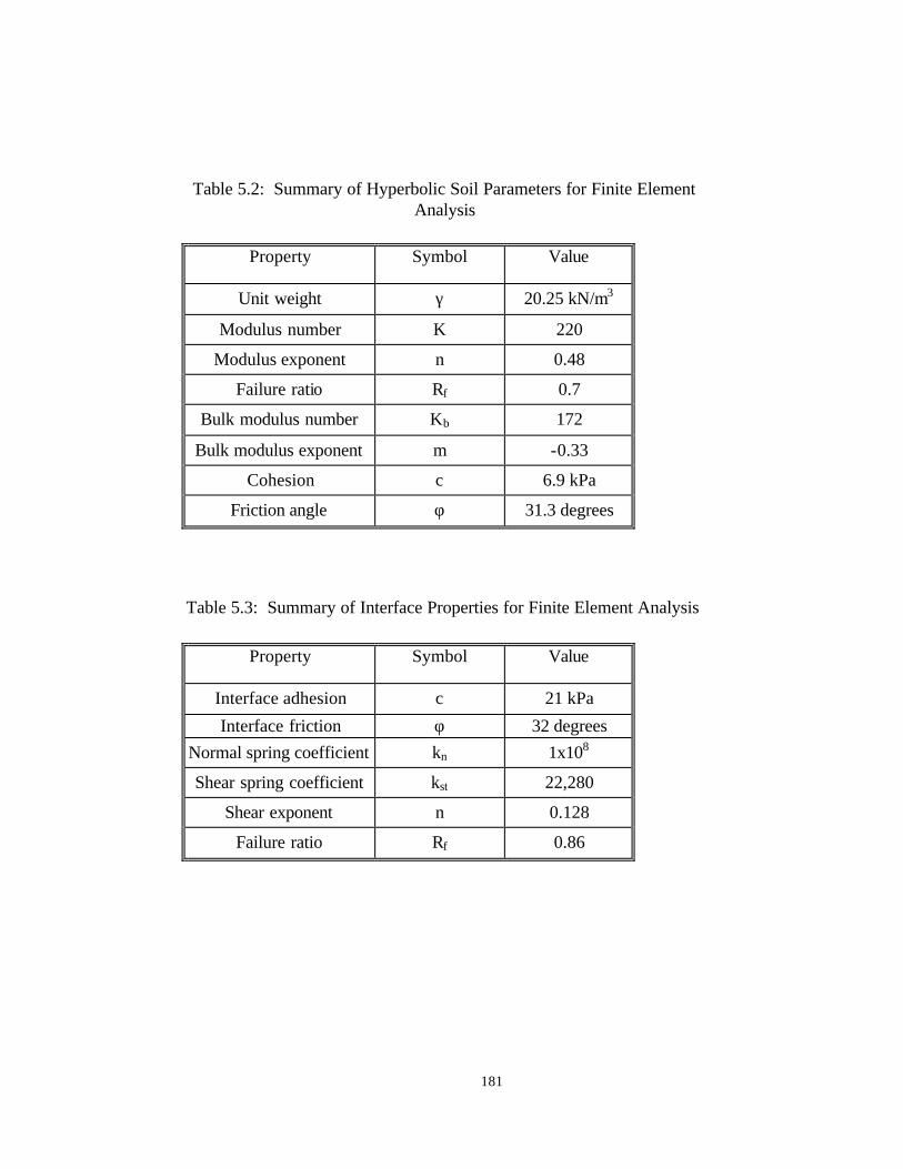
181

Table 5.2: Summary of Hyperbolic Soil Parameters for Finite Element

Analysis

Property Symbol Value

Unit weight γ 20.25 kN/m3

Modulus number K 220

Modulus exponent n 0.48

Failure ratio Rf 0.7

Bulk modulus number Kb 172

Bulk modulus exponent m -0.33

Cohesion c 6.9 kPa

Friction angle φ 31.3 degrees

Table 5.3: Summary of Interface Properties for Finite Element Analysis

Property Symbol Value

Interface adhesion c 21 kPa

Interface friction φ 32 degrees Normal spring coefficient kn 1x108

Shear spring coefficient kst 22,280

Shear exponent n 0.128

Failure ratio Rf 0.86

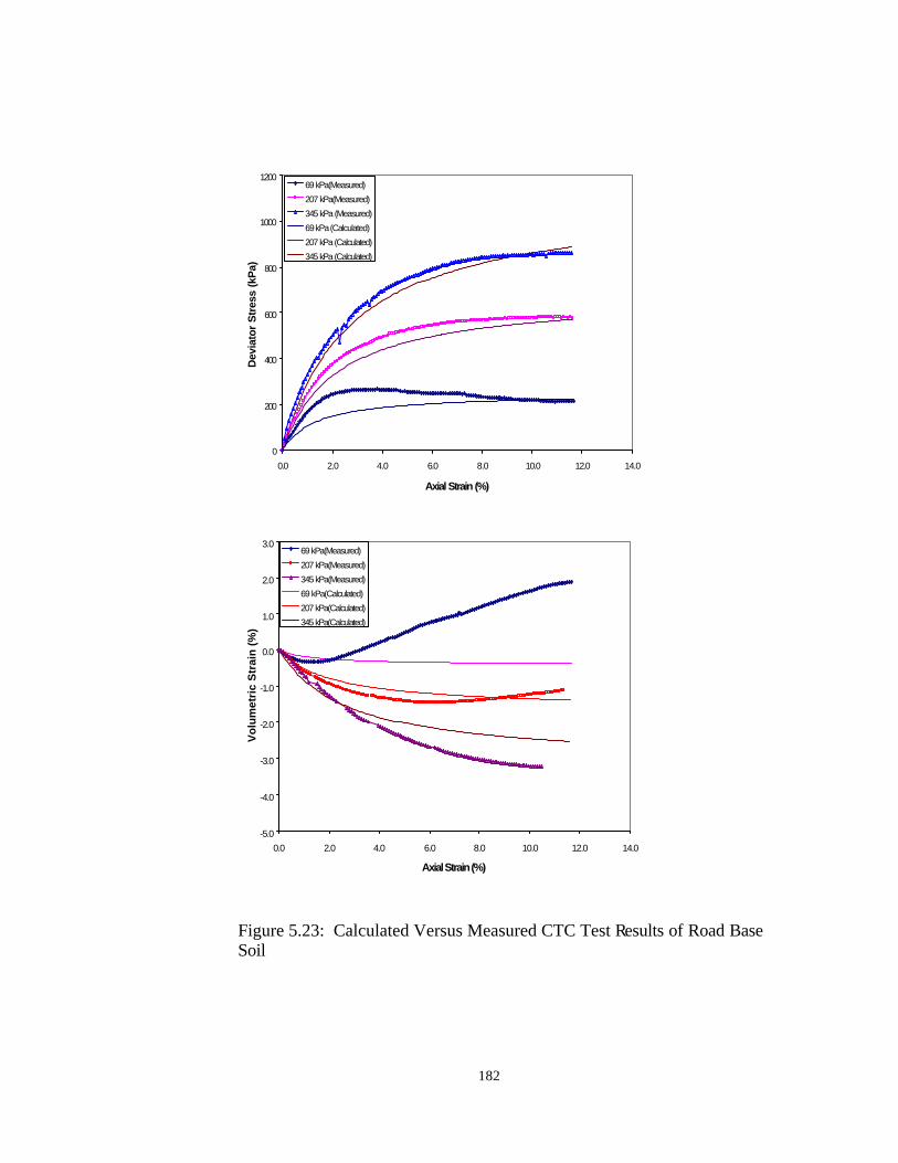
182

Figure 5.23: Calculated Versus Measured CTC Test Results of Road Base Soil

0

200

400

600

800

1000

1200

0.0 2.0 4.0 6.0 8.0 10.0 12.0 14.0

Axial Strain (%)

Devi

ator

Stre

ss (k

Pa)

69 kPa(Measured)207 kPa(Measured)345 kPa (Measured)69 kPa (Calculated)207 kPa (Calculated)345 kPa (Calculated)

-5.0

-4.0

-3.0

-2.0

-1.0

0.0

1.0

2.0

3.0

0.0 2.0 4.0 6.0 8.0 10.0 12.0 14.0

Axial Strain (%)

Volu

met

ric S

trai

n (%

)

69 kPa(Measured)207 kPa(Measured)345 kPa(Measured)69 kPa(Calculated)207 kPa(Calculated)345 kPa(Calculated)

183

Figure 5.24: Calculated Versus Measured DS Test Results of Road Base Soil and Amoco 2044 Interface

0

50

100

150

200

250

300

0 1 2 3 4 5 6 7 8

Horizontal Displacement (mm)

Shea

r Str

ess

(kPa

)

86 kPa (Measured)195 kPa (Measured)358 kPa (Measured)86 kPa (Calculated)195 kPa (Calculated)358 kPa (Calculated)

Normal Stress

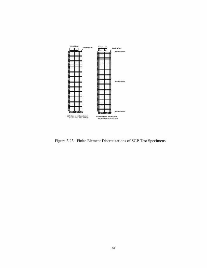
184

Figure 5.25: Finite Element Discretizations of SGP Test Specimens

Loading PlateVertical Load

Reinforcement

Reinforcement

Vertical Load

Reinforcement

Loading Plate

(a) Finite element discretization of a soil mass in the SGP test

(b) Finite Element Discretization of a GRS mass in the SGP test

185

Figure 5.26: Measured and Calculated Vertical and Average Horizontal Displacements of Test P-M-RB

0

2

4

6

8

10

12

14

0 5 10 15 20

Displacement (mm)

Vert

ical

Loa

d (k

N)

Vertical (Measured)Vertical (Calculated)Avg. Horizontal (Measured)Avg. Horizontal (Calculated)

186

Figure 5.27: Measured and Calculated Vertical and Average Horizontal Displacements of Test P-M-(RB+2044)

0

2

4

6

8

10

12

14

16

18

0 5 10 15 20 25 30

Displacement (mm)

Verti

cal L

oad

(kN

)

Vertical (Measured)Vertical (Calculated)Avg. Horizontal (Measured)Avg. Horizontal (Calculated)

187

Figure 5.28: Calculated Strain Distributions in the Middle Reinforcement Layer

0.00

0.02

0.04

0.06

0.08

0.10

0.12

0.14

0.16

0.18

0.20

0 20 40 60 80 100 120

Distance from Center Line (mm)

Rei

nfor

cem

ent S

trai

n (%

)

2 kN4 kN6 kN

188

5.4.6 Stresses in GRS Mass in the SGP Test The stress distributions of the soil mass with and without reinforcement in the SGP test were compared. Figures 5.29, 5.30, and 5.31 present, respectively, the vertical, horizontal, and shear stress distributions at a vertical load of 6 kN. The stress intensity, shown by different colors, in half of the specimen geometry is illustrated. It is seen that the vertical stress distributions of the specimen with and without reinforcement are almost identical, whereas the horizontal and the shear stress distributions are distinctly different. The vertical stress at any given height was approximately the sum of the confining pressure and the vertical stresses due to the external load, the self-weight of the soil, the weight of the loading plate, and the seating load.

The horizontal stresses were rather uniform in the specimen without reinforcement and were equal to the confining pressure of 34.5 kPa. With the presence of three reinforcement layers, the horizontal stress distribution was quite different. A high horizontal stress of about 50 kPa occurred adjacent to the reinforcement and gradually reduced away from the reinforcement location.

The shear stress in the specimen without reinforcement was nearly zero. Some shear stresses occurred near the reinforcement in the specimen with reinforcement. On each reinforcement layer, the shear stresses vary along the horizontal direction with a minimum value of almost zero at the centerline and a maximum value of about 10 kPa at the end. Such a shear stress distribution is similar to the calculated shear stress distribution by Ashwamy et al. (1998) of reinforced-soil specimens in a conventional triaxial compression test.

It is to be noted that the shear stresses at mid-height between two vertically adjacent reinforcement layers are almost zero. This behavior has been referred to as a shear stress reversal by Smith (1977). Adib (1988) and Sawicki (1998) applied the shear stress reversal concept in their simplified models to calculate reinforcement tensions in reinforced-soil retaining walls. In this study, the shear stress reversal concept was employed in the development of the SPR model to estimate the deformation behavior. This will be described in detail in Chapter 6.

To quantify the reinforcing effect, a minor principal stress ratio is introduced. The minor principal stress ratio is defined as the ratio of the compressive minor principal stress in a specimen with reinforcement to that of the specimen without reinforcement. The minor principal stress ratio gives a direct indication of the increase in the minor principal stresses resulting from the reinforcement.

Figure 5.32 shows a distribution of the minor principal stress ratio. As shown in Figure 5.32, the maximum value of minor principal stress ratio of about 1.4 to 1.5 occurred near the reinforcement and reduced with the distance from the reinforcement location. The minor principal stress ratio was near unity (i.e., no reinforcing effects) around the middle area of two adjacent reinforcement layers.

189

Based on the finite element analyses, it can be concluded that the presence of the reinforcement altered the horizontal and shear stress distributions but not the vertical stress distribution. The horizontal and shear stresses increased significantly near the reinforcement and resulted in an increase of the minor principal stress. By increasing the minor principal stress, deformation stiffness and shear strength of the soil were also increased. The reinforcing effect, as quantified by the minor principal stress ratio, was the largest near the reinforcement and reduced with increasing distance from the reinforcement.

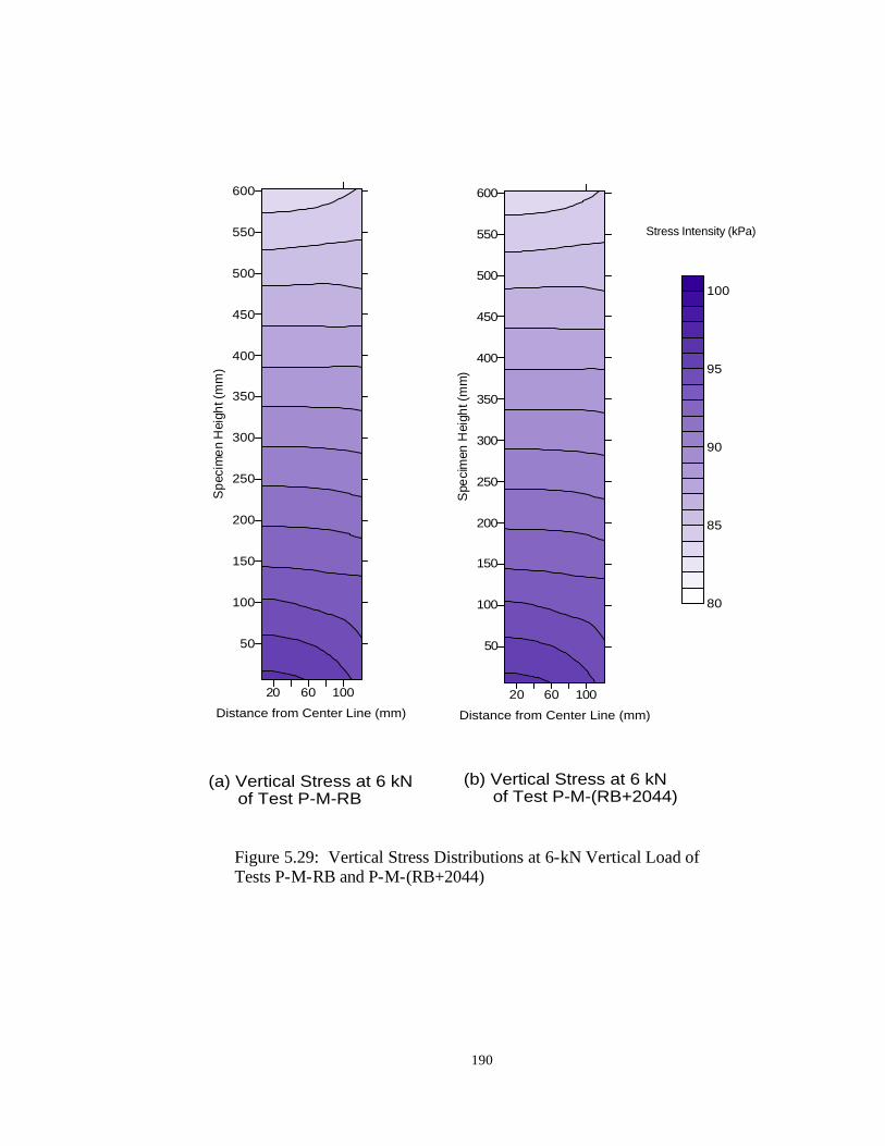
190

Figure 5.29: Vertical Stress Distributions at 6-kN Vertical Load of Tests P-M-RB and P-M-(RB+2044)

20 60 100Distance from Center Line (mm)

50

100

150

200

250

300

350

400

450

500

550

600

Spec

imen

Hei

ght (

mm

)

80

85

90

95

100

(b) Vertical Stress at 6 kN of Test P-M-(RB+2044)

20 60 100Distance from Center Line (mm)

50

100

150

200

250

300

350

400

450

500

550

600

Spec

imen

Hei

ght (

mm

)

(a) Vertical Stress at 6 kN of Test P-M-RB

Stress Intensity (kPa)

191

Figure 5.30: Horizontal Stress Distributions at 6-kN Vertical Load of Tests P-M-RB and P-M-(RB+2044)

20 60 100Distance from Center Line (mm)

50

100

150

200

250

300

350

400

450

500

550

600

Spe

cim

en H

eigh

t (m

m)

34

38

42

46

50

(b) Horizontal Stress at 6 kN of Test P-M-(RB+2044)

Stress Intensity (kPa)

20 60 100Distance from Center Line (mm)

50

100

150

200

250

300

350

400

450

500

550

600

Spe

cim

en H

eigh

t (m

m)

(a) Horizontal Stress at 6 kN of Test P-M-RB

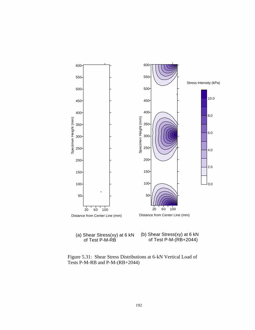
192

Figure 5.31: Shear Stress Distributions at 6-kN Vertical Load of Tests P-M-RB and P-M-(RB+2044)

20 60 100Distance from Center Line (mm)

50

100

150

200

250

300

350

400

450

500

550

600

Spec

imen

Hei

ght (

mm

)

0.0

2.0

4.0

6.0

8.0

10.0

(b) Shear Stress(xy) at 6 kN of Test P-M-(RB+2044)

Stress Intensity (kPa)

20 60 100Distance from Center Line (mm)

50

100

150

200

250

300

350

400

450

500

550

600

Spe

cim

en H

eigh

t (m

m)

(a) Shear Stress(xy) at 6 kN of Test P-M-RB

193

Figure 5.32: Distribution of Minor Principal Stress Ratio at 6-kN Vertical Load of Test P-M-(RB+2044)

20 60 100Distance from Center Line (mm)

50

100

150

200

250

300

350

400

450

500

550

600Spe

cimen

Height

(mm)

1.00

1.10

1.20

1.30

1.40

1.50

Stress Ratio

194

5.5 Summary and Concluding Remarks A total of 11 SGP tests were carried out to investigate the behavior of a GRS mass subject to monotonic loading and unloading-reloading cycles. The SGP tests were conducted on the soil mass with and without reinforcement. The monotonic-loading test program was designed to examine the reinforcing effects during monotonic loading and to provide a reference for an assessment of the effects of preloading on GRS masses. The unloading-reloading test program was designed to examine the effects of preloading, different types of the unloading-reloading cycles (i.e., RL-Z and RL-PS paths), the effects of preloading magnitude, and the reinforcing effects during the unloading-reloading cycles. The finite element analyses were conducted to examine the stress distribution in a GRS mass in the SGP test. The monotonic- loading SGP tests showed that: 1. Due to the reinforcing effects imposed by the reinforcement, a soil mass with

reinforcement had higher stiffness and strength than without reinforcement. The vertical stiffness of the soil mass with reinforcement was about 30% higher than without reinforcement.

2. Some vertical and horizontal deformations were required to mobilize the reinforcing effects. Before the reinforcing effect was fully mobilized, the soil mass with and without reinforcement showed comparable deformations. For the Road Base soil mass with or without reinforcement, the required vertical and horizontal displacements to fully mobilize the reinforcing effect were 2.0 mm and 0.5 mm, respectively.

The unloading-reloading SGP tests showed that: 1. With preloading, the stiffness of the GRS mass increased significantly. For the

GRS mass comprising the Ottawa sand and Amoco 2044 geotextile reinforcement, the stiffness increased by factors of 3 to 7 in the vertical direction, and about 7 in the horizontal direction. For the GRS mass comprising the Road Base soil and Amoco 2044 geotextile reinforcement, the stiffness increased by factors of 2 to 5 in the vertical direction, and about 3 in the horizontal direction.

2. The magnitude of the preloading load level did not appear to affect the reloading stiffness except at the initial stage of the reloading path. During the initial stage of the reloading path, the rebounding deformation continued if the test specimen was unloaded from a high preloading load level to a zero- load level. Similar rebounding deformation behavior was also observed in the FHWA pier after unloading had completed.

3. The RL-PS path showed higher vertical reloading stiffness than the RL-Z path. The vertical reloading stiffness increased with increasing prestressed load level. In the horizontal direction, the stiffness of both the RL-Z and RL-PS paths was comparable.

195

4. The unloading and reloading curves of the multiple unloading-reloading at working load levels nearly coincided with one another. This behavior was also observed in the FHWA pier and the Black Hawk abutments.

5. The reinforcing effect was insignificant during the reloading path. 6. Preloading did not appear to affect the load carrying capacity of the GRS mass.

The finite element analysis showed that: 1. The presence of the reinforcement layers in the soil mass altered the horizontal

and shear stress distributions but not the vertical stress distribution. 2. The horizontal and shear stresses increased significantly near the reinforcement

and resulted in an increase of the minor principal stress. With the increasing minor principal stress, the deformation stiffness and shear strength of the soil were subsequently increased. The reinforcing effect, as quantified by the increase of the minor principal stress, was the largest near the reinforcement and reduced with the increasing distance from the reinforcement.

196

6. Simplified Preloading-Reloading Model for GRS Mass

A simplified model, referred to as the simplified preloading-reloading (SPR) model, was developed and is presented in this chapter. The purpose of the model is to provide a simple model for estimating deformation of a GRS mass subject to monotonic loading or preloading and subsequent reloading.

The SPR model consists of two principal modules: a load-transfer module and a deformation module. The load-transfer module can be used to calculate the average stresses in a GRS mass. The deformation module can be used to calculate the vertical and horizontal deformations of a GRS mass on the basis of the average stresses from the load-transfer module.

6.1 Load-Transfer Module

The purpose of the load-transfer module is to quantify the stress distribution in a GRS mass. The stress distributions in a GRS mass are typically non-uniform, as illustrated by the finite element analyses in Section 5.4.6. The load-transfer module assumes the uniform stresses. The uniform stresses determined by the module can be considered as average vertical and horizontal stresses (σv andσh ) in a GRS mass. The average stresses are determined by a load-transfer analysis developed from the elastic analysis of an idealized plane-strain GRS mass.

The following sections present the load-transfer analysis, verification of the load-transfer analysis with experimental and numerical results, and formulations of the average stresses in a GRS mass.

6.1.1 Load-Transfer Analysis

The load-transfer analysis is based on the elastic analysis of reinforcement tensions in a GRS mass. Figure 6.1 shows the idealized geometry of a plain-strain GRS mass. The reinforced-soil mass consists of a horizontal reinforcement layer embedded in a soil at mid-height. The reinforced-soil mass is subjected to uniform compressive vertical pressure (Pv) and horizontal pressure (Ph) along the top and lateral surfaces. Tensile forces in the reinforcement are induced by the stresses developed in the soil from externally applied pressures, Pv and Ph. Figure 6.2 shows differential elements of the soil and the reinforcement for the equilibrium equations.

197

Figure 6.1: An Idealized Plane-Strain GRS Mass for the SPR Model

SOIL

REINFORCEMENTAs = Sv

L

SOIL

Pv

Ph

198

Figure 6.2: Equilibrium of Differential Soil and Reinforcement Elements (Reproduced from Hermann and Al-Yassin, 1978)

Soil Element

dx

τ(x)

σx

Reinforcement Element

τ(x)

dx

σx + dσx

F(x) + dFF(x)

199

The following presents the elastic solution for the reinforcement tension. It is extended from the solution given by Adib (1988), who modified the solution by Hermann and Al-Yassin (1978). The following assumptions were made in obtaining the solutions. 1) The soil and the reinforcement behave as linear, isotropic, and elastic materials. 2) The soil and the reinforcement are linked together through an elastic soil-

reinforcement interface. 3) There is no axial force at the end of the reinforcement (i.e., F(x=L) = 0). 4) The horizontal stress in the soil and the reinforcement tension do not vary in the

vertical direction. 5) The vertical stress in the soil is constant and equal to the boundary vertical

pressure. 6) There is no relative horizontal displacement in the soil along the vertical

direction. Let U(x) = displacement function of the soil in the x direction

V(x) = displacement function of the reinforcement in the x direction W(x) = displacement function of the soil- reinforcement interface element in the x-direction

)()()( xVxUxW −= [6.1]

Equilibrium Equations For the condition given in Figure 6.1, the following equilibrium equations can

be derived. The normal stress is taken as positive for tension and negative for compression. 1) Equilibrium of the differential soil element as shown in Figure 6.2:

dxxWpkAd isx ⋅⋅⋅=⋅ )(σ [6.2(a)]

or

s

ix

AxWpk

dxd )(⋅⋅

=σ

[6.2(b)]

where ki = stiffness of the interface element p = perimeter of the reinforcement that is in contact with the soil As = area of the soil = Sv Note that the term ki⋅W(x) is the shear stress along the interface. 2) Equilibrium of the differential reinforcement element:

dxxWpkxdF i ⋅⋅⋅−= )()( [6.3(a)]

200

or

)()( xWpkdx

xdFi ⋅⋅−= [6.3(b)]

Stress-Strain Relationships 1. Soil For plane strain condition (with z-axis being the longitudinal direction):

0=zε [6.4(a)]

)( yxsz σσνσ +⋅= [6.4(b)]

In x-direction:

( ))(1yzsx

sx E

σσνσε +⋅−⋅= [6.5(a)]

where νs = Poisson’s ratio of the soil Es = Young’s modulus of the soil Subsitute Eq. 6.4(b) into Eq. 6.5(a) to yield:

( )ysssxs

x Eσνννσε ⋅+⋅−−⋅⋅= )1()1(1 2 [6.5(b)]

Rearrange Eq. 6.5(b),

xs

sy

s

sx

Eε

νσ

νν

σ ⋅−

+⋅−

=)1()1( 2 [6.5(c)]

2. Reinforcement The reinforcement tension can be expressed as:

rrr EAxF ε⋅⋅=)( [6.6]

Strain-Displacement Relationships 1. Soil Soil strain in the x-direction:

dxxdU

x)(

=ε [6.7(a)]

where Er = Young’s modulus of the reinforcement Ar = cross-sectional area of the reinforcement

201

εr = strain in the reinforcement Substitute Eq. 6.7(a) into Eq. 6.5(c) and differentiate with respect to x to yield:

2

2

2)(

)1( dxxUdE

dxd

s

sx ⋅−

=ν

σ [6.7(b)]

2. Reinforcement Reinforcement strain:

dxxdV

r)(

=ε [6.8(a)]

Substitute Eq. 6.8(a) into Eq. 6.6 and differentiate with respect to x to yield:

2

2 )()(dx

xVdEAdx

xdFrr ⋅⋅= [6.8(b)]

or

−⋅⋅= 2

2

2

2 )()()(dx

xWddx

xUdEA

dxxdF

rr [6.8(c)]

From Eq.6.2(b) and Eq. 6.7(b):

2

2

2)(

)1()(

dxxUdE

AxWpk

dxd s

s

ix ⋅−

=⋅⋅

=ν

σ [6.9(a)]

Rearrange Eq. 6.9(a):

)()1()( 2

2

2

xWpkAEdx

xUdi

ss

s ⋅⋅⋅⋅

−=

ν [6.9(b) ]

From Eq. 6.3(b) and Eq. 6.8(c):

−⋅⋅=⋅⋅−= 2

2

2

2 )()()(

)(dx

xWddx

xUdEAxWpk

dxxdF

rri [6.10]

Substitute Eq. 6.9(b) into Eq. 6.10 to yield:

−⋅⋅⋅

⋅−

⋅⋅=⋅⋅− 2

22 )()()1(

)(dx

xWdxWpkAE

EAxWpk iss

srri

ν [6.11(a)]

202

Rearrange Eq. 6.11(a):

)()1(1)( 2

2

2

xWAEEA

pkdx

xWdss

s

rri ⋅

⋅

−+

⋅⋅⋅=

ν [6.11(b)]

Introduce

⋅

−+

⋅⋅⋅=

ss

s

rri AEEA

pk)1(1 2

2 να [6.12]

Eq. 6.11(b) can be expressed as:

)()( 22

2

xWdx

xWd⋅= α [6.13]

The solution of Eq. 6.13 can be expressed in the following form:

)sinh()cosh()( xbxaxW ⋅⋅+⋅⋅= αα [6.14]

Substitute Eq. 6.14 into Eq. 6.9(b) to solve for the soil displacement function:

( ))sinh()cosh()1()( 2

2

2

xbxapkAEdx

xUdi

ss

s ⋅⋅+⋅⋅⋅⋅⋅⋅

−= αα

ν [6.15]

Introduce

pkAE i

ss

s ⋅⋅⋅

−=

)1( 2νβ [6.16]

Eq. 6.15 can be expressed as:

( ))sinh()cosh()(2

2

xbxadx

xUd⋅⋅+⋅⋅⋅= ααβ [6.17]

and

203

( ) dxcxbxadxdxdx

xUdxU +⋅+⋅⋅+⋅⋅⋅== ∫∫ )sinh()cosh()()( 22

2

αααβ [6.18]

where a, b, c, and d are integration constants.

The above derivations were taken from Hermann and Al-Yassin (1978) and Adib (1988). The extension of the solution is presented below.

Impose the following four boundary conditions to solve for U(x): 1. The displacement of the soil at x = 0 is zero:

U(x=0) = 0 2. The displacement of the interface element at x = 0 is zero:

W(x=0) = 0 3. The force in the reinforcement at x = L is zero:

F(x=L) = 0 4. The horizontal stress in the soil at x = L is the lateral boundary pressure:

σx(x=L) = -Ph

From condition (2) and Eq. 6.14,

0=a [6.19(a)]

From condition (1) and Eq. 6.18,

0=d [6.19(b)]

From condition (3) and Eq. 6.6,

)1()cosh( 2αβ

αα −⋅⋅⋅⋅= Lbc [6.19(c)]

From condition (4) and Eq. 6.5(c),

)cosh()1(

)1

(2

LbE

PPcs

sv

s

sh ⋅⋅

⋅−

−⋅

⋅

−+−= α

αβν

νν

[6.19(d)]

Solve for b and c from Eq. 6.19(c) and 6.19(d),

)cosh(1)1(

)1

(2

LEPPb

s

shv

s

s

⋅⋅⋅

−⋅

−⋅

−=

ααν

νν

[6.19(e)]

204

)1()1(

)1

( 2

2

αβν

νν

−⋅−

⋅

−⋅

−=

s

shv

s

s

EPPc [6.19(f)]

The Force in the Reinforcement From Eq. 6.6,

−⋅⋅=⋅⋅=

dxxdW

dxxdUEAEAxF rrrrr

)()()( ε [6.20(a)]

The force in the reinforcement can be expressed as:

⋅⋅

−⋅

−⋅

−⋅

−⋅

−⋅⋅=

)cosh()cosh(11

)1()

1()( 2

2

Lx

EPPEAxF

s

shv

s

srr α

ααβν

νν [6.20(b)]

The maximum force in the reinforcement occurs at x = 0 and can be expressed as:

⋅

−⋅

−⋅

−⋅

−⋅

−⋅⋅=

)cosh(111

)1()

1( 2

2

max LEPPEAF

s

shv

s

srr αα

βνν

ν [6.20(c)]

The Horizontal Stress in the Soil From Eq. 6.5(c):

dxxdUE

PE

s

sv

s

sx

s

sy

s

sx

)()1(

)1

()1(

)1

( 22 ⋅−

+⋅−

−=⋅−

+⋅−

=νν

νε

νσ

νν

σ [6.21(a)]

The horizontal stress in the soil can be expressed as:

−+

⋅⋅

⋅⋅

−⋅

−+⋅

−

−= )1()cosh()cosh(

)1

(1 22 α

βαα

αβ

νν

νν

σLx

PPP hvs

sv

s

sx [6.21(b)]

6.1.2 Comparison of Load-Transfer Analysis with Experimental and Numerical Analysis Results of the APSR Test

To evaluate validity of the load-transfer analysis presented in Section 6.1.1, the closed-form solution for reinforcement tension (Eq. 6.20(b)) was used to predict the reinforcement tension in the APSR cell developed by Whittle et al. (1992). The results of the load-transfer analysis were compared with the experimental results by Whittle et al. (1992) and the numerical results from finite-element analyses of the APSR cell by Abramento and Whittle (1993).

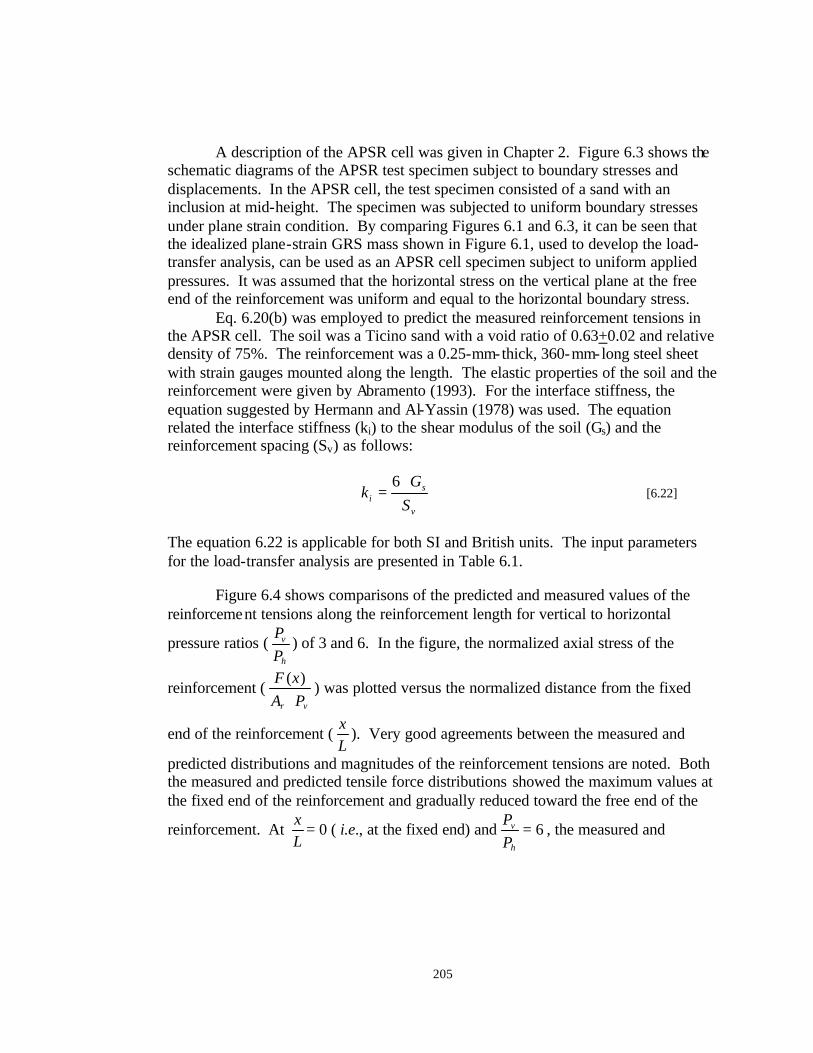
205

A description of the APSR cell was given in Chapter 2. Figure 6.3 shows the schematic diagrams of the APSR test specimen subject to boundary stresses and displacements. In the APSR cell, the test specimen consisted of a sand with an inclusion at mid-height. The specimen was subjected to uniform boundary stresses under plane strain condition. By comparing Figures 6.1 and 6.3, it can be seen that the idealized plane-strain GRS mass shown in Figure 6.1, used to develop the load-transfer analysis, can be used as an APSR cell specimen subject to uniform applied pressures. It was assumed that the horizontal stress on the vertical plane at the free end of the reinforcement was uniform and equal to the horizontal boundary stress.

Eq. 6.20(b) was employed to predict the measured reinforcement tensions in the APSR cell. The soil was a Ticino sand with a void ratio of 0.63+0.02 and relative density of 75%. The reinforcement was a 0.25-mm-thick, 360-mm-long steel sheet with strain gauges mounted along the length. The elastic properties of the soil and the reinforcement were given by Abramento (1993). For the interface stiffness, the equation suggested by Hermann and Al-Yassin (1978) was used. The equation related the interface stiffness (ki) to the shear modulus of the soil (Gs) and the reinforcement spacing (Sv) as follows:

v

si S

Gk

⋅=

6 [6.22]

The equation 6.22 is applicable for both SI and British units. The input parameters for the load-transfer analysis are presented in Table 6.1.

Figure 6.4 shows comparisons of the predicted and measured values of the reinforcement tensions along the reinforcement length for vertical to horizontal

pressure ratios (h

v

PP ) of 3 and 6. In the figure, the normalized axial stress of the

reinforcement (vr PA

xF⋅

)( ) was plotted versus the normalized distance from the fixed

end of the reinforcement (Lx ). Very good agreements between the measured and

predicted distributions and magnitudes of the reinforcement tensions are noted. Both the measured and predicted tensile force distributions showed the maximum values at the fixed end of the reinforcement and gradually reduced toward the free end of the

reinforcement. At Lx = 0 ( i.e., at the fixed end) and 6=

h

v

PP , the measured and

206

predicted normalized axia l stresses were 358. At Lx = 0.4 of the same pressure ratio,

the measured and predicted normalized axial stresses were 320 and 307, respectively. The load-transfer analysis was also performed to predict the maximum

normalized axial stress (i.e., at Lx = 0) of a hypothetical APSR test specimen for

different material properties and reinforcement lengths. The predictions were compared with the values computed from the finite element analyses conducted by Abramento and Whittle (1993) using the ABAQUS finite element program. It was assumed in the finite element analysis that the reinforcement was fully bonded with the soil.

Table 6.3 shows a comparison of the maximum normalized axial stress

of the reinforcement (vr PA

F⋅

max ) for different material properties and reinforcement

lengths. The properties for the finite element analysis and the load-transfer analysis are given in Table 6.2. The difference between values calculated from the load-transfer analysis and the finite element analysis was within 5%. These experimental and numerical comparisons validate the load-transfer analysis for analyzing reinforcement tension in the GRS mass.

207

Figure 6.3: Schematic Diagrams of the APSR Cell (After Whittle et al., 1991)

208

Table 6.1: Input Parameters for Load-Transfer Analysis of the APSR Test Specimen (Data from Abramento, 1993)

Property Symbol Unit Value

Shear modulus of soil Gs kN/m2 6,000

Poisson's ratio of soil νs 0.35

Cross-sectional area of soil As m2 0.57

Reinforcement modulus Er kN/m2 2.07x108

Cross-sectional area of reinforcement Ar m2 2.54x10-4

Reinforcement length L m 0.36

Perimeter of reinforcement p m 2

209

Figure 6.4: Predicted and Measured Normalized Reinforcement Stress Distributions in the APSR Cell

0

50

100

150

200

250

300

350

400

0 0.2 0.4 0.6 0.8 1

Normalized Distance from the Fixed End of the Reinforcementx/L

Nor

mal

ized

Axi

al S

tres

s in

the

Rei

nfor

cem

ent,

(F(x

)/Ar)/

P v

Measured, Pv/Ph=3Predicted, Pv/Ph=3Measured, Pv/Ph=6Predicted, Pv/Ph=6

210

Table 6.2: Reference Properties for Comparison of Maximum Normalized Reinforcement Stress for Table 6.3 (Data from Whittle et al., 1991)

Property Symbol Unit Value

Young's modulus of soil Es kN/m2 104

Poisson's ratio of soil νs 0.3

Cross-sectional area of soil As m2 0.57

Stiffness ratio of soil and reinforcement Er/Gs 103

Reinforcement thickness t m 10-3

Reinforcement length L m 1.0 Perimeter of reinforcement P m 2.0

Applied pressure ratio Pv/Ph 10

211

Table 6.3: Comparison of Maximum Normalized Reinforcement Stress (vr PA

F⋅

max ),

from Finite Element Analysis and Load-Transfer Analysis

L = 0.5 m

Er/Gs νs = 0.3 νs = 0.5 Finite Load-Transfer Finite Load-Transfer Element Analysis Element Analysis Analysis Analysis

102 10.9 10.8 21.8 21.5 103 63.6 63.6 135 136 104 115 115 264 268

L = 100 m

Er/Gs νs = 0.3 νs = 0.5 Finite Load-Transfer Finite Load-Transfer Element Analysis Element Analysis Analysis Analysis

102 10.9 10.8 21.8 21.6 103 74.4 71.2 163 156 104 168 161 438 418

212

6.1.3 Average Stresses in GRS Mass Based on the load-transfer analysis, the average vertical and horizontal

stresses in a GRS mass are introduced. The average vertical and horizontal stresses are needed in the deformation module for estimating deformations of a GRS mass. Uniform vertical and horizontal stresses are assumed for the average stresses.

The average vertical stress,σv, is assumed to be equal to the boundary vertical pressure, i.e.,

vv P=σ [6.23]

Compressive stress is taken as positive and tensile stress as negative. The average horizontal stress,σh, is defined as:

L

dxxL

x

h

∫= 0

)(σσ [6.24(a)]

By substituting σx(x) from Eq. 6.21(b) into Eq. 6.24(a) and performing integration, the average horizontal stress is obtained as:

−

⋅⋅

⋅+⋅

−⋅

−−⋅

−= )1

)tanh((1)

1()

1( 2 L

LPPP hv

s

sv

s

sh

αα

αβ

νν

νν

σ [6.24(b)]

6.2 Deformation Module This section presents the deformation module of the SPR model. The average stress-displacement diagram is first described, followed by the equations used to calculate the vertical and horizontal displacements. 6.2.1 Average Stress-Displacement Diagram The average stress-displacement diagram is a conceptual diagram that provides a graphical representation of the average stress path and the corresponding displacements of an idealized plane-strain GRS mass under monotonic loading and unloading-reloading cycles. The average vertical stress ( vs ) was plotted versus the average horizontal pressure ( hs ), and the corresponding vertical displacement (δv) and horizontal displacement (δh). All the average stresses in the average stress-displacement diagram are in compression. Figure 6.5 shows the average stress-displacement diagrams of a GRS mass subject to monotonic loading. Initially, a GRS mass is subjected to initial applied boundary pressures of Pv,i and Ph,i. The initial average vertical and horizontal stresses ( ih,iv , s and s ) in the average stress diagram are equal to Pv,i and Ph,i, respectively.

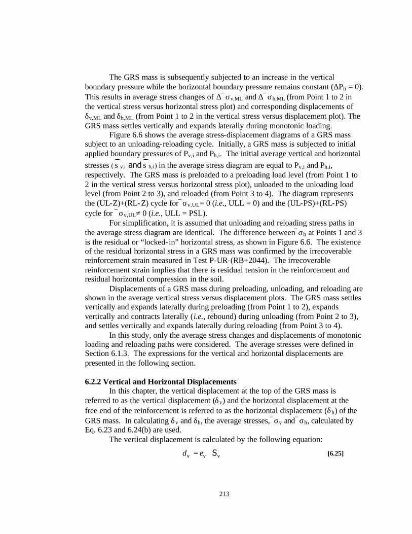
213

The GRS mass is subsequently subjected to an increase in the vertical boundary pressure while the horizontal boundary pressure remains constant (∆Ph = 0). This results in average stress changes of ∆σv,ML and ∆σh,ML (from Point 1 to 2 in the vertical stress versus horizontal stress plot) and corresponding displacements of δv,ML and δh,ML (from Point 1 to 2 in the vertical stress versus displacement plot). The GRS mass settles vertically and expands laterally during monotonic loading.

Figure 6.6 shows the average stress-displacement diagrams of a GRS mass subject to an unloading-reloading cycle. Initially, a GRS mass is subjected to initial applied boundary pressures of Pv,i and Ph,i. The initial average vertical and horizontal stresses ( ih,iv , s and s ) in the average stress diagram are equal to Pv,i and Ph,i, respectively. The GRS mass is preloaded to a preloading load level (from Point 1 to 2 in the vertical stress versus horizontal stress plot), unloaded to the unloading load level (from Point 2 to 3), and reloaded (from Point 3 to 4). The diagram represents the (UL-Z)+(RL-Z) cycle forσv,UL= 0 (i.e., ULL = 0) and the (UL-PS)+(RL-PS) cycle for σv,UL≠ 0 (i.e., ULL = PSL).

For simplification, it is assumed that unloading and reloading stress paths in the average stress diagram are identical. The difference betweenσh at Points 1 and 3 is the residual or “locked- in” horizontal stress, as shown in Figure 6.6. The existence of the residual horizontal stress in a GRS mass was confirmed by the irrecoverable reinforcement strain measured in Test P-UR-(RB+2044). The irrecoverable reinforcement strain implies that there is residual tension in the reinforcement and residual horizontal compression in the soil. Displacements of a GRS mass during preloading, unloading, and reloading are shown in the average vertical stress versus displacement plots. The GRS mass settles vertically and expands laterally during preloading (from Point 1 to 2), expands vertically and contracts laterally (i.e., rebound) during unloading (from Point 2 to 3), and settles vertically and expands laterally during reloading (from Point 3 to 4).

In this study, only the average stress changes and displacements of monotonic loading and reloading paths were considered. The average stresses were defined in Section 6.1.3. The expressions for the vertical and horizontal displacements are presented in the following section.

6.2.2 Vertical and Horizontal Displacements

In this chapter, the vertical displacement at the top of the GRS mass is referred to as the vertical displacement (δv) and the horizontal displacement at the free end of the reinforcement is referred to as the horizontal displacement (δh) of the GRS mass. In calculating δv and δh, the average stresses,σv andσh, calculated by Eq. 6.23 and 6.24(b) are used. The vertical displacement is calculated by the following equation:

vvv S⋅= εδ [6.25]

214

where Sv = height of the GRS mass

εv = vertical strain of the GRS mass and given as:

⋅

−−⋅

−= h

s

sv

s

sv E

σν

νσ

νε

)1()1( 2

[6.26]

The horizontal displacement is calculated by integrating the reinforcement strain along the reinforcement length.

dxEAxF

dxxL L

rrrh ∫ ∫ ⋅

==0 0

)()(εδ [6.27(a)]

By subsituting F(x) from Eq. 20(b) into Eq. 6.27(a) and performing integration, δh is obtained as:

⋅

−⋅

−⋅

−⋅

−⋅

−=

αα

αβν

νν

δ)tanh(

11

)1

( 2

2 LL

EPP

s

shv

s

sh [6.27(b)]

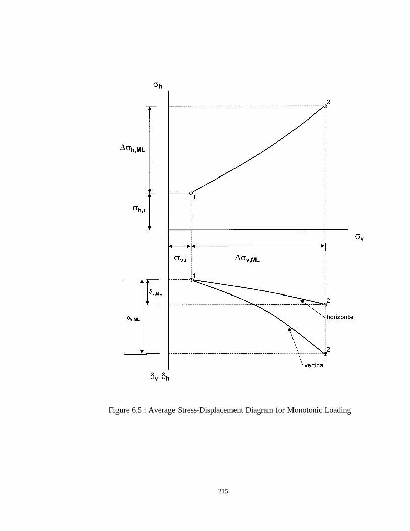
215

Figure 6.5 : Average Stress-Displacement Diagram for Monotonic Loading

216

Figure 6.6: Average Stress-Displacement Diagram for Unloading and Reloading

217

6.3 Comparison of SPR Model Prediction with SGP Test Results To evaluate the SPR model, the SPR model was used to predict the vertical and horizontal displacements of the GRS mass in the SGP test, referred to as the SGP-GRS mass. The following sections present the application of the SPR model to the SGP test, the selection of material and interface properties, and the comparison. 6.3.1 Application of SPR Model to SGP Test

Due to some differences in the configurations of the idealized plane-strain GRS mass (Figure 6.1) and the SGP-GRS mass (Figure 6.7), some assumptions were made to apply the SPR model on the SGP-GRS mass. From the finite element analysis of the SGP-GRS mass presented in Chapter 5, it was learned that a zero-shear plane can be assumed on the horizontal plane at mid-height between two vertically adjacent layers of reinforcement. The zero-shear plane assumption allowed a simplified analysis of the average stresses in the SGP-GRS mass. The SGP-GRS mass was divided into three layers, referred to as Layers T (top), M (middle), and B (bottom), with the zero-shear planes as border lines (see Figure 6.7).

The average stresses of each layer were determined separately by the SPR model. The average vertical stress of each layer was the sum of the vertical boundary pressure (Pv) and the vertical stress from the self-weight of the soil at mid-height of the layer. The boundary vertical pressure was assumed to be uniform along the horizontal plane. This assumption was justified based on the result of the finite element analysis (see Figure 5.30). The average horizontal stress was calculated by Eq. 6.24(b). Note that the reinforcement perimeter (p) of Layers T and B was half of the perimeter of Layer M since the latter has twice the contact areas between the soil and the reinforcement.

The vertical displacement of each layer was calculated by Eq. 6.25. The vertical displacement of the SGP-GRS mass was the sum of the vertical displacements of Layers T, M, and P. The horizontal displacement at mid-height of the SGP-GRS mass was equal to the horizontal displacement of Layer M and was given by Eq. 6.27(b).

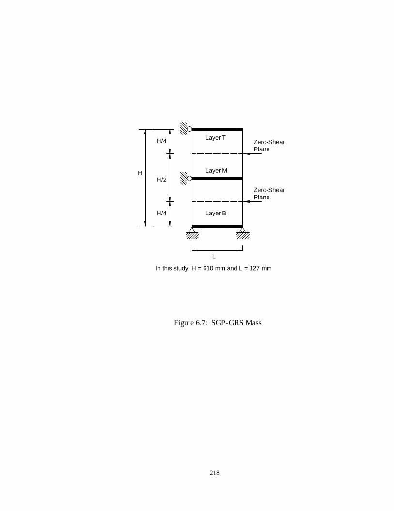
218

Figure 6.7: SGP-GRS Mass

In this study: H = 610 mm and L = 127 mm

Layer B

Layer M

Layer T

H/4

HH/2

H/4

L

Zero-Shear Plane

Zero-Shear Plane

219

6.3.2 Determination of Material and Interface Properties Determination of the soil, geosynthetic, and interface properties for the SPR model are presented below. The subscripts ML and RL represent monotonic loading path and reloading path, respectively.

6.3.2.1 Soil For monotonic loading, a hyperbolic average stress-strain relationship based

on the hyperbolic soil model proposed by Duncan et al. (1980) was used. The tangential Young’s modulus and Poisson’s ratio for each load increment are given as follows.

n

a

MLha

MLh

MLhMLvfMLs P

PKc

RE

⋅⋅⋅

⋅⋅+⋅⋅−⋅−⋅

−= ,2

,

,,,

sin2cos2)()sin1(

1σ

φσφσσφ

[6.28]

⋅−=

MLs

MLsMLs B

E

,

,, 6

5.0ν [6.29]

where Bs,ML = bulk modulus of the soil during monotonic loading 1

,,

m

a

MLhabMLs P

PKB

⋅⋅=

σ [6.30]

The parameters for the soil model were determined by the procedure recommended by Duncan et al. (1980) and calibrated with the results of the SGP test without reinforcement. The calibration was conducted by using the SPR model assuming very small reinforcement stiffness to simulate the soil mass without reinforcement.

For the reloading path, the reloading modulus, Eq. 5.5, suggested by Duncan et al. (1980) was first examined. Based on Eq. 5.5, the reloading modulus for a soil is only a function of the minor principal stress (σ3), or the confining pressure in the CTC test. This implies that the reloading modulus at a given confining pressure is a constant whether the specimen is reloaded from a zero- load level (RL-Z path) or a prestressed load level (RL-PS path). However, from the CTC test results, the reloading modulus of the RL-PS path was consistently higher than that of the RL-Z path (see Figures 3.19 and 3.20). Therefore, the reloading modulus given by Duncan et al. (1980) was considered inadequate to model the reloading deformation of the GRS mass.

Tatsuoka and his associates at the University of Tokyo performed extensive laboratory tests on rectangular prism soil specimens to determine the elastic Young’s modulus of soils. The elastic modulus in a certain direction (i.e., vertical or

220

horizontal) was obtained at very small strains (on the order of 0.001%) by applying very small cyclic stresses in that direction. The strains were measured by local deformation transducers (Goto et al., 1991) to eliminate effects of bedding error. They have found that the tangent elastic Young’s modulus in a certain direction is a unique function of the operative normal stress in that direction (Kohata et al., 1994; Tatsuoka and Kohata, 1995; Hoque et al., 1995). Tatsuoka et al. (1997) proposed the following empirical relationship for the vertical elastic Young’s modulus based on the laboratory test results by Dong et al. (1994).

m

o

vo

ee EE

⋅=

σσ

)( [6.31]

where Ee is the elastic Young’s modulus in the vertical direction at a vertical stress σv, (Ee)o is the value of Ee when σv is equal to a reference value σo, and m is the power number. The tests were conducted at confining pressures of 19.6 kPa and 78.5 kPa. In this study, the reloading modulus from the CTC tests was examined. It was found that a power law can be used to relate the reloading modulus (ERL) to the vertical unloading stress (σv,UL) as shown in Eq. 6.32. The vertical unloading stress was the sum of the confining pressure and the deviator stress at the end of the unloading path.

q

a

ULvrefRLRL P

EE

⋅= ,σ

[6.32]

where Eref

RL = reference reloading modulus, ERL when σv,UL = Pa q = exponent number However, it was found that Eq. 6.32 cannot account for the increasing of

reloading stiffness due to prestress in the SGP test. Based on the SGP test results, an empirical coefficient λ was introduced to account for the effect of the prestressed load level (PSL). Eq. 6.32 was modified as follows:

q

a

ULvrefRLRL P

EE

⋅⋅= ,σ

λ [6.33]

where λ = empirical coefficient to account for the effect of prestress

level (λ = 1 for the RL-Z path, PSL = 0) σv,UL = average vertical unloading stress

221

The parameters ErefRL and q were determined from the CTC tests and

calibrated with the results of the SGP test without reinforcement (Tests P-UR-S and P-UR-RB) under the RL-Z path (PSL = 0 and λ = 1). The parameter λ was obtained from the results of the SGP test without reinforcement (Test P-UR-RB) under the RL-PS path. For the Sand specimen, Test P-UR-(S+2044)-3 was used to determine the parameter λ. The unloading threshold load, as described in Section 5.2, was used as a criterion for differentiating the RL-Z path and the RL-PS path. The SPR model assumed the RL-Z path (i.e., λ = 1) when the unloading load level was less than the unloading threshold load, and otherwise assumed the RL-PS path.

The reloading Poisson’s ratio (νs,RL ) is calculated from the following equation:

⋅−=

RLs

RLsRLs B

E

,

,, 6

5.0ν [6.34]

where Bs,RL = bulk modulus of the soil during reloading

2

,,,

m

a

RLhaRLbRLs P

PKB

⋅⋅=

σ [6.35]

The isotropic compression test may be conducted to determine change of bulk

modulus due to preloading. However, such a test was not available for the soils in this study. It was assumed that Kb,ML= Kb,RL and m1=m2.

A summary of the soil properties for the SGP-GRS mass is presented in Table 6.4.

222

Table 6.4: Summary of Soil Properties for the SPR Model (a) Ottawa Sand

Property Symbol Value

Unit weight (kN/m3) γ 16.8

Monotonic Loading Modulus number K 350

Modulus exponent n 0.5 Failure ratio Rf 0.7

Bulk modulus number Kb 675 Bulk modulus exponent m1 0.4

Cohesion (kPa) c - Friction angle (degree) φ 40.6

Reloading Path Reference modulus number Eref

RL 70000 Reloading modulus exponent q 0.2

Prestress- level coefficient λ 2.0 Bulk modulus number Kb,RL 675

Bulk modulus exponent m2 0.4

223

Table 6.4: Summary of Soil Properties for the SPR Model (Continued) (b) Road Base Soil

Property Symbol Value

Unit weight (kN/m3) γ 20.25 Monotonic Loading

Modulus number K 220 Modulus exponent n 0.48

Failure ratio Rf 0.7 Bulk modulus number Kb 172

Bulk modulus exponent m1 -0.33 Cohesion (kPa) c 6.9

Friction angle (degree) φ 31.3 Reloading Path

Reference modulus number ErefRL 27000

Reloading modulus exponent q 0.58

Prestress- level coefficient λ 1.4

Bulk modulus number Kb,RL 172

Bulk modulus exponent m2 -0.33

224

6.3.2.2 Geosynthetic The reinforcement stiffness (Er ⋅Ar) for the SPR model can be obtained from

the load-extension test of the geosynthetic. The secant stiffness (J) in the range of the expected reinforcement strain should be used. The SPR model allows the use of different values of reinforcement stiffness (Er) during the preloading and reloading paths. In the SGP tests, the measured reinforcement strains of Amoco 2044 reinforcement were relatively small (in the range of 0 to 0.5%). An unloading-reloading LE test was conducted to determine the reloading modulus at small strains of Amoco 2044 geosynthetic. The test result is shown in Figure 6.8. It shows that, for strain less than 0.5%, the secant stiffness of the preloading and reloading paths is approximately the same. The stiffness of 1,000 kN/m was used for the Amoco 2044 reinforcement.

6.3.2.3 Soil-Geosynthetic Interface

The interface stiffness (ki) in the SPR model can be determined from direct shear tests of the interface between the soil and geosynthetic reinforcement. Based on the results of the interface direct shear tests conducted in this study (see Section 3.6.5), the following equations are proposed.

1

1,

p

a

nwdsMLi P

kk

⋅⋅=

σγ [6.36]

2

2,

p

a

nwdsRLi P

kk

⋅⋅=

σγ [6.37]

where ki,ML and ki,RL = monotonic-loading and reloading interface stiffness kds1 and kds2 = interface stiffness number

p1 and p2 = interface exponent γw = unit weight of water

σn = normal stress on the interface The monotonic- loading interface stiffness (ki,ML) can be determined from a plot of K50/γw versus σn/Pa on a log- log scale. In the same fashion, the reloading interface stiffness (ki,RL) can be determined from a plot of KRL/γw ratio versus the σn/Pa on a log-log scale. A summary of the interface properties for the SGP-GRS mass is presented in Table 6.5.

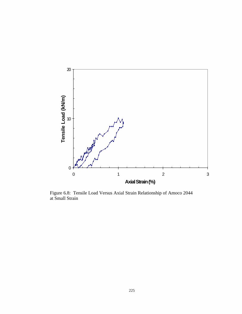
225

Figure 6.8: Tensile Load Versus Axial Strain Relationship of Amoco 2044 at Small Strain

0

10

20

0 1 2 3

Axial Strain (%)

Tens

ile L

oad

(kN

/m)

226

Table 6.5: Summary of Interface Properties for the SPR Model

Symbol Value

Ottawa Sand + Amoco 2044 Reinforcement

ML interface stiffness number kds1 17,450

ML interface stiffness exponent p1 0.28

RL interface stiffness number kds2 25,290

RL interface stiffness exponent p2 0.24 Road Base Soil + Amoco 2044

Reinforcement

ML interface stiffness number kds1 11,110

ML interface stiffness exponent p1 0.45

RL interface stiffness number kds2 19,690

RL interface stiffness exponent p2 0.31

227

6.3.3 Calculation Example The change in the average stresses and the corresponding change in the

vertical and horizontal displacements of the SGP-GRS mass were formulated in an incremental form to simulate the stress-dependent properties of the soil and the interface. Note that during the vertical load application, the boundary horizontal pressure remained constant (∆Ph = 0).

vv P∆=∆σ [6.38]

−

⋅⋅

⋅+⋅

∆⋅

−−∆⋅

−=∆ )1

)tanh((1)

1()

1( 2 L

LPP v

s

sv

s

sh

αα

αβ

νν

νν

σ [6.39]

vh

s

sv

s

sv S

E⋅

∆⋅

−−∆⋅

−=∆ σ

νν

σν

δ)1(

)1( 2

[6.40]

⋅−⋅

−⋅

−⋅

∆⋅

−=∆

αα

αβν

νν

δ)tanh(

11

)1

( 2

2 LL

EP

s

sv

s

sh [6.41]

The calculations of the average stresses and displacements were performed by a spreadsheet program. An example calculation for Layer M of the SGP-GRS mass is presented in Table 6.6. The spreadsheet consists of the input in the upper area and the computation in the lower area. The properties of the soil, the reinforcement, and the interface must be provided as the input.

Columns 1 to 33 performed calculations based on Eq. 6.38 to 6.41. Columns 1 and 2 are the vertical boundary pressures. Column 3 is the vertical stress resulting from self-weight of the soil. Column 4 is the confining pressure applied prior to the vertical load from the loading device. Columns 5 and 6 give the average vertical and horizontal stresses of each step. Columns 7 and 8 are the average vertical and horizontal stresses used to calculate the soil and the interface properties of each increment. Columns 9 to 22 are the calculation parameters. Column 23 gives the average horizontal stress as a result of the incremental vertical boundary pressure. The horizontal stress value in Column 23 is added to the average horizontal stress in the previous step. Note that iterations are needed in each increment for calculation of the average horizontal stress. This is because the soil and the interface properties are a function of the average horizontal stress which, in turn, is a function of the properties of the soil and the interface. Columns 24 to 28 calculate the vertical displacement. Columns 29 to 33 calculate the horizontal displacement.

228

Table 6.6: Calculation Example of SPR Model for SGP-GRS Mass

Calculating Vertical and Horizontal Displacements of SGP-GRS Mass by the SPR Model

By: Kanop Ketchart, Dept. of Civil Eng., U of Colorado at Denver

Input

Soil: Middle Layer f = 31.3 degree c = 6.9 kPa g = 20.25 kN/m3 z mid-

height = 0.3 m

K = 220 n = 0.48 Kb = 172 m = -0.33 β = ki*p*(1-n2)/EsAs Eref

RL = 27000 a2 = k ip(1/ErAr+(1-n2)/EsAs) q = 0.58 Rf = 0.7

Reinforcement: Stiffness ErAr = 1000 kN/m Interface: kds = 11110 Perimeter p = 2 m p = 0.45 Vertical spacing

Sv = AS = 0.3 m

Length L = 0.127 m

229

Table 6.6: Calculation Example of SPR Model for SGP-GRS Mass (Continued)

1 2 3 4

Step i Increment ∆ Pv Pv γ∗z PC

(mid-height) (kPa) (kPa) (kPa) (kPa)

1 0.000 6.075 34.5 1 9

2 9.000 6.075 34.5 2 9

3 18.000 6.075 34.5

5 6 7 8 9 10 σv σh σv,avg σh,avg (sv,avg-sh,avg) (sv,avg-sh,avg)f

=(Pv+γ∗z+PC) = σh,i+∆ σh, i-j =(σv,j+σv,i)/2 =(σh,j+σh,i)/2

(kPa) (kPa) (kPa) (kPa) (kPa) (kPa) 40.58 34.50

45.08 34.80 10.28 99.71 49.58 35.09

54.08 35.44 18.63 101.10 58.58 35.79

11 12 13 14 15 16 SL Ei Es=Et B ν ki

(kPa) (kPa) (kPa) (kN/m3)

0.103093831 13,254 11,410 24,368 0.42 77,622

0.18430997 13,372 10,144 24,221 0.43 84,249

230

Table 6.6: Calculation Example of SPR Model for SGP-GRS Mass (Continued)

17 18 19 20

Step i Increment a2 a β ν /(1-ν) 1 1 192.52 13.8752 37.27719 0.729982 2 2 213.62 14.61571 45.12177 0.754998 3

21 22 23 b/a2 (tanh(α*L)/α*L-1) ∆ σh, i-j

(kPa)

0.193626 -0.465004548 0.592

0.211226 -0.486947193 0.699

231

Table 6.6: Calculation Example of SPR Model for SGP-GRS Mass (Continued)

Vertical Displacement 24 25 26 27 28

Step i Increment ∆sv ∆sh ∆ εver εver S total

(kPa) (kPa) (mm) 1 0 0 1 9.00 0.592 0.000617218 2 0.00061722 0.1851654 2 9.00 0.699 0.00068064 3 0.00129786 0.38935751

Horizontal Displacement (sum of two sides) 29 30 31 32 33

Step i Increment (1−ν2)/Es (1-b/a2) (L+tanh(α*L)/α) ∆ δhor δhor

(mm) (mm) 1 0.0000 1 7.204E-05 0.806374 0.059055578 0.045075 2 0.0451 2 8.034E-05 0.788774 0.061842293 0.053256 3 0.0983

232

6.3.4 Comparison of SPR Model Prediction with SGP Test Results The predicted and measured displacements of the SGP-GRS mass under the

monotonic loading and reloading paths are presented. The SPR model was not used to predict the displacements near the failure load of the specimen because there was a high possibility of local failure in some areas of the specimen near the failure load. The SPR model, which is based on average stress fields, cannot model local soil failure. A stress level (SL) of 0.85 was set as the threshold level above which the SPR model is deemed not applicable.

Figures 6.9 and 6.10 show a comparison of the predicted and measured displacements of the GRS masses with the Sand and Road Base soil under monotonic loading. The predicted and measured displacements are in very good agreement. At 42.5-kN vertical load, the predicted vertical and horizontal displacements of the GRS mass with the Sand were 9.5 mm and 2.1 mm as compared with the measured values of 9.9 mm and 2.2 mm, respectively. At 13-kN vertical load, the predicted vertical and horizontal displacements of the GRS mass with the Road Base soil were 5.4 mm and 0.9 mm as compared with the measured values of 6.1 mm and 1.1 mm, respectively.

A comparison of the predicted and measured displacements of the GRS masses under RL paths are presented in Figures 6.11 to 6.14. The reloading displacements were referenced to the deformed shape of the specimen at the end of the unloading path.

Figures 6.11 and 6.12 show the displacements under, respectively, the RL-Z and RL-PS paths for the GRS masses with the Sand. The reduced vertical reloading stiffness at the initial RL-Z path, as described in Section 5.2, was modeled empirically base on the observations. At the vertical load of zero to 0.05⋅PLL of the RL-Z path, the reloading modulus of the soil was empirically reduced to 30% (i.e., 70% reduction) of the reloading modulus calculated by Eq. 6.24. The reduction of reloading modulus was not used in the RL-PS path. The predicted and measured values for the Sand specimen during reloading paths are considered acceptable with some discrepancies in the horizontal displacements during initial RL-Z path. At a vertical load of 20 kN, the predicted and measured vertical displacements were, respectively, 1.34 mm and 1.23 mm for the RL-Z path, and 0.56 mm and 0.56 mm for the RL-PS path. The predicted and measured horizontal displacements were, respectively, 0.16 mm and 0.02 mm for the RL-Z path, and 0.02 mm and 0.05 mm for the RL-PS path.

The displacements under the RL-Z path of the GRS mass with the Road Base soil are shown in Figure 6.13. Figure 6.14 and 6.15 shows the displacements under the RL-PS path. During the initial stage of the RL-Z path, the specimen continued to rebound in both vertical and horizontal directions. To model this behavior, an empirical procedure was performed. Negative values of predicted displacements were used to represent rebounding deformation. From observation, negative vertical

233

displacements occurred from the vertical load of zero to 0.05⋅PLL and negative horizontal displacements from the vertical load of zero to 0.3⋅PLL. The RL-PS paths show the rebounding deformation only in the horizontal direction. The empirical procedure for the rebounding deformation was also used for horizontal displacements of the RL-PS path. With the empirical procedure for rebounding deformation, the SPR model appears to give a good overall simulation of the displacements in the GRS mass with the Road Base soil during RL-Z and RL-PS paths. At a vertical load of 4 kN, the predicted and measured vertical displacements were, respectively, 0.73 mm and 0.82 mm for the RL-Z path, 0.53 mm and 0.56 mm for the RL-PS1 path, and 0.47 mm and 0.33 mm for the RL-PS2 path. The predicted and measured horizontal displacements were, respectively, -0.05 mm and -0.02 mm for the RL-Z path, 0.02 mm and 0.03 mm for the RL-PS1 path and 0.01 mm and 0.01 mm for the RL-PS2 path.

234

Figure 6.9: Predicted Versus Measured Vertical and Horizontal Displacements of Test P-M-(S+2044)

0

10

20

30

40

50

60

0 5 10 15 20 25 30

Displacement (mm)

Verti

cal L

oad

(kN

)

Measured (Vertical)Predicted (Vertical)Measured (Horizontal)Predicted (Horizontal)

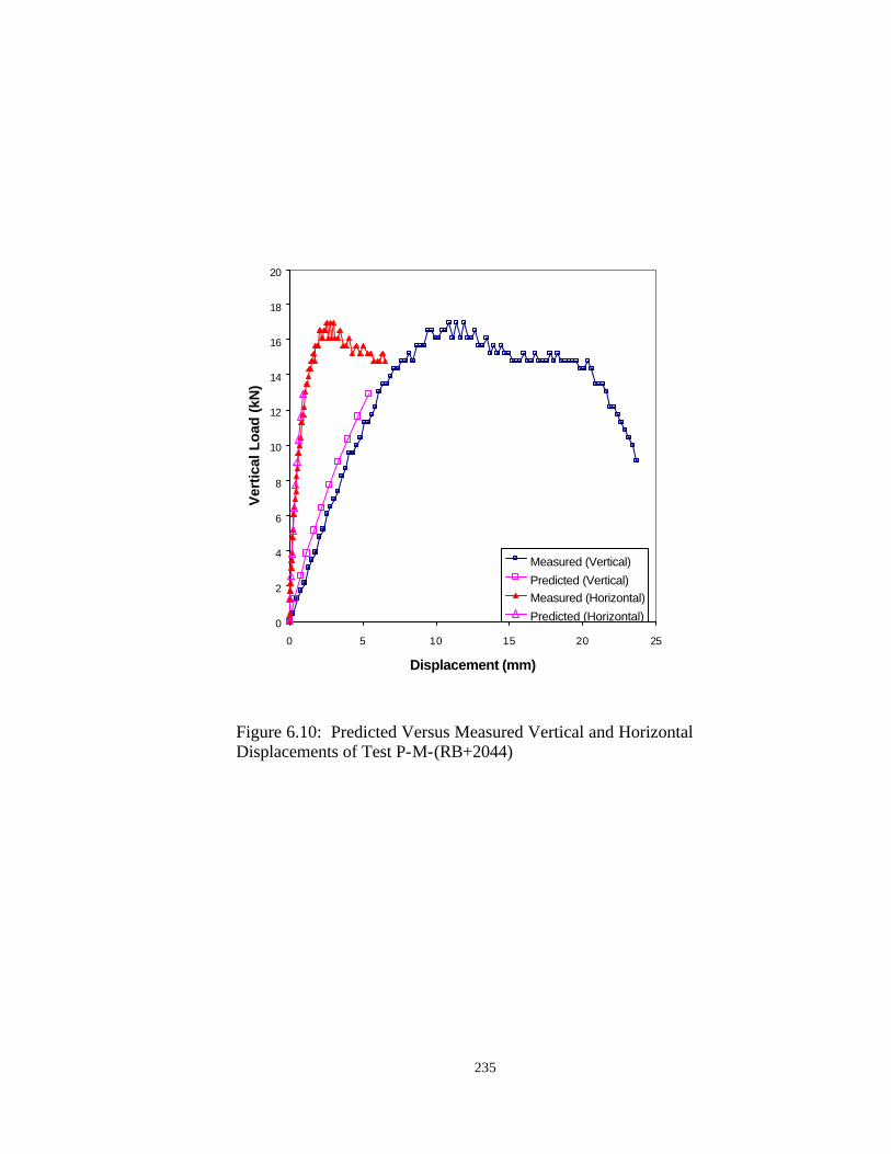
235

Figure 6.10: Predicted Versus Measured Vertical and Horizontal Displacements of Test P-M-(RB+2044)

0

2

4

6

8

10

12

14

16

18

20

0 5 10 15 20 25

Displacement (mm)

Verti

cal L

oad

(kN

)

Measured (Vertical)Predicted (Vertical)Measured (Horizontal)Predicted (Horizontal)

236

Figure 6.11: Predicted Versus Measured Reloading Vertical and Horizontal Displacements of Test P-UR-(S+2044), RL-Z path

0

5

10

15

20

25

30

35

40

45

50

0 1 2 3 4 5

Displacement (mm)

Verti

cal L

oad

(kN

)

Measured (Vertical)Predicted (Vertical)Measured (Horizontal)Predicted (Horizontal)

237

Figure 6.12: Predicted Versus Measured Reloading Vertical and Horizontal Displacements of Test P-UR-(S+2044), RL-PS path

0

5

10

15

20

25

0 0.5 1 1.5 2 2.5 3

Displacement (mm)

Verti

cal L

oad

(kN

)

Measured (Vertical)Predicted (Vertical)Measured (Horizontal)Predicted (Horizontal)

238

Figure 6.13: Predicted Versus Measured Reloading Vertical and Horizontal Displacements of Test P-UR-(RB+2044), RL-Z path

0

2

4

6

8

10

12

-0.5 0 0.5 1 1.5 2 2.5 3

Displacement (mm)

Verti

cal L

oad

(kN

)

Measured (Vertical)Predicted (Vertical)Measured (Horizontal)Predicted (Horizontal)

239

Figure 6.14: Predicted Versus Measured Reloading Vertical and Horizontal Displacements of Test P-UR-(RB+2044), RL-PS1 path

0

1

2

3

4

5

6

-0.5 0 0.5 1 1.5 2

Displacement (mm)

Verti

cal L

oad

(kN

)

Measured (Vertical)Predicted (Vertical)Measured (Horizontal)Predicted (Horizontal)

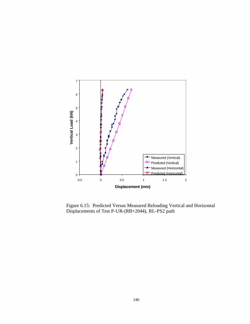
240

Figure 6.15: Predicted Versus Measured Reloading Vertical and Horizontal Displacements of Test P-UR-(RB+2044), RL-PS2 path

0

1

2

3

4

5

6

7

-0.5 0 0.5 1 1.5 2

Displacement (mm)

Verti

cal L

oad

(kN

)

Measured (Vertical)Predicted (Vertical)Measured (Horizontal)Predicted (Horizontal)

241

6.4 Parametric Study on Deformation of GRS Mass A parametric study was carried out by the SPR model to examine the influences of the soil, reinforcement, and interface on the deformation behavior of a GRS mass. The baseline properties for the materials used in the parametric study are presented in Table 6.7. These properties were used in all displacement calculations except the parameter being investigated. Three parameters were investigated: the soil stiffness (Es), the reinforcement stiffness (Er⋅Ar), and the interface stiffness (ki).

The displacement ratio and the stiffness ratio are introduced to simplify the presentation of the results. The displacement ratio is defined as the ratio of the displacement of a GRS mass with the varied parameter to the displacement of the GRS mass with the baseline properties. The stiffness ratio is defined as the ratio of the varied parameter to the baseline value of the stiffness.

Figure 6.16 shows the relationships between vertical displacement ratio and stiffness ratios of the soil, the reinforcement, and the interface. Each stiffness ratio was varied from 1 to 10. The figures show that the reduction of the vertical displacements was far more pronounced with increasing soil stiffness than reinforcement stiffness. The change in the interface stiffness shows little effect. At a stiffness ratio of 2, the vertical displacement ratios due to the increase of soil, reinforcement, and interface stiffnesses were, respectively, 0.5, 0.98, and 1.0. At a stiffness ratio of 5, the vertical displacement ratios due to the increase of soil, reinforcement, and interface stiffnesses were, respectively, 0.2, 0.96, and 1.0.

Figure 6.17 shows the relationships between horizontal displacement ratio and the stiffness ratio of the soil, reinforcement, and interface. Similar to the vertical displacement, the horizontal displacements reduced with increasing soil and reinforcement stiffnesses. Increasing the soil stiffness has a more significant effect than increasing the reinforcement stiffness. The change in the interface stiffness shows little effect. At a stiffness ratio of 2, the horizontal displacement ratios due to the increase of soil, reinforcement, and interface stiffness were, respectively, 0.55, 0.8, and 1.0. At a stiffness ratio of 5, the horizontal displacement ratios due to the increase of soil, reinforcement, and interface stiffness were, respectively, 0.25, 0.5, and 1.0.

These results have an important practical implication in selecting a method to reduce the settlement of a GRS mass. Either employing a stiffer reinforcement or increasing the soil stiffness can reduce the settlement of a GRS mass. Figure 6.16 can be used as a guide for reducing settlement. This finding supports the use of a preloading technique for reducing post-construction settlement of a GRS structure.

242

Table 6.7: Properties for the Baseline GRS Mass

Property Symbol Unit Value

Young's Modulus of soil Es kN/m2 104

Poisson's ratio of soil ν 0.3 Cross sectional area of soil As m2 0.3

Reinforcement stiffness ErAr kN/m 103

Reinforcement length L m 3 Perimeter of reinforcement p m 2.0

Interface stiffness ki kN/m3 3x104

Applied pressure ratio Pv/Ph 5

243

Figure 6.16: Vertical Displacement Ratio Versus Stiffness Ratio Relationships

0

0.2

0.4

0.6

0.8

1

1.2

1.4

1 2 3 4 5 6 7 8 9 10 11 12

Stiffness Ratio

Vert

ical

Dis

plac

emen

t Rat

io

Soil StiffnessReinforcement StiffnessInterface Stiffness

244

Figure 6.17: Horizontal Displacement Ratio Versus Stiffness Ratio Relationships

0

0.2

0.4

0.6

0.8

1

1.2

1.4

1 2 3 4 5 6 7 8 9 10 11 12

Stiffness Ratio

Hor

izon

tal D

ispl

acem

ent R

atio

Soil StiffnessReinforcement StiffnessInterface Stiffness

245

6.5 Summary and Concluding Remarks A simplified preloading-reloading (SPR) model was developed and presented

in this chapter. The purpose of the model was to provide a simple tool for estimating the deformation of a GRS mass subject to monotonic loading or preloading and subsequent reloading. The SPR model consists of two principal modules: a load-transfer module and a deformation module. The load-transfer module is based on the elastic analysis of the load-transfer mechanism in an idealized plane-strain GRS mass. The load-transfer module assumes uniform stresses, referred to as the average stresses, in a GRS mass. The deformation module used the average stresses determined from the load-transfer module to calculate the vertical and horizontal displacements of the GRS mass.

The SPR model was evaluated by comparing its results with experimental and numerical analysis results of the APSR test (Whittle et al., 1992; Abramento and Whittle, 1993) and the SGP test results conducted in this study. The comparison yielded satisfactory results. Although further verification is still needed, the SPR model appears to be a valid tool for estimating the deformation of GRS masses.

To examine the influences of increasing stiffness of soil, reinforcement, and interface on the deformation behavior of a GRS mass, a parametric study was conducted by the SPR model. The parametric study showed that vertical displacement of the GRS mass was significantly reduced by increasing soil stiffness. The effect of increasing reinforcement stiffness was much smaller, whereas the effect of increasing the interface stiffness was negligible. This finding supports the benefits of employing a preloading technique in reducing post-construction settlement of GRS structures.

246

7. Correlation Between SGP Test and Preloaded GRS Structure

This chapter describes correlations between the results of SGP tests and preloaded GRS structures. Two preloaded GRS structures and the corresponding SGP tests were examined. The first was the FHWA pier (Adams, 1997) and the performance test conducted by the second-generation SGP test prior to construction. The second was the Black Hawk abutments (Wu et al., 1999) and the modified SGP test. Both SGP tests were conducted with the same soil and reinforcement as those used in the preloaded GRS structures. The correlations were made in terms of normalized values of loads and displacements.

It should be noted that deformation behavior of a GRS structure depends on various factors such as soil, reinforcement, reinforcement spacing, facing rigidity, geometry, soil placement condition, and construction sequence. The SGP test is capable of simulating the soil, the reinforcement, and the reinforcement spacing only. An absolute correlation, therefore, is not feasible. The attempt here is to establish the correlation for a construction protocol and a facing type (segmental concrete blocks with no pins for the FHWA pier and rock-faced type for the Black Hawk abutment). 7.1 FHWA Pier The project description of the FHWA pier was presented in Chapter 2. The pier was load-tested on July 3, 1996, and July 23, 1996, which were referred to as the first and the second load tests. For each load test, The loading sequences consisted of two paths: preloading and reloading paths. In the first load test, the GRS pier was incrementally loaded up to 900 kPa and unloaded to zero. In the reloading path, the load was increased to 415 kPa and unloaded to zero. Note that the maximum loads in both preloading and reloading paths were much higher than the suggested maximum contact pressure of 200 kPa for mechanically stabilized bridge abutments (Elias and Christopher, 1997). In the second load test, the GRS pier was incrementally loaded up to 780 kPa and unloaded to zero. In the reloading path, the pier was loaded up to 780 kPa. 7.1.1 Load Test Results

The results of the first and the second load tests were compared to examine effects of preloading. In this section, the term “vertical displacement” refers to the average settlement of the loading pad; the term “horizontal displacement” refers to the horizontal displacement at mid-height of the wall faces; and the reloading displacement was referenced to the deformed shape of the pier at the end of unloading. The preloading and reloading paths of the first load test were designated as the preloading and first reloading paths. The preloading and reloading paths of the second load test were designated as the second and third reloading paths.

247

Figure 7.1 shows the relationship between the vertical applied pressure and displacements of the FHWA pier in the four loading paths. It can be seen that preloading reduced the vertical displacements of the FHWA pier. The vertical displacement at 200 kPa was 14.6 mm in the preloading path and 8.1 mm in the first reloading path. Figure 7.1 also shows that the reduction in vertical settlement was insignificant in the subsequent reloading paths (i.e., in the second and third reloading paths). Figure 7.1 shows the vertical applied pressure versus horizontal displacement relationships in the four loading paths. It shows that the horizontal movement for all loading paths was practically the same until the vertical pressure exceeds 400 kPa. The horizonatal displacements reduced somewhat due to preloading when the vertical pressure was higher than 400 kPa. The preloading effect in the horizontal direction, after the pressure exceeded 400 kPa, was not as significant as in the vertical direction. The horizontal displacement at 580 kPa was 13.9 mm in the preloading path and 11.1 mm in the second reloading path. 7.1.2 SGP Test Results

The test specimen of the SGP test was prepared by employing the same soil and geosynthetic reinforcement as those used in actual construction of the FHWA pier. The test was conducted prior to construction of the pier by Sam Yu and Damin Shi at the University of Colorado at Denver. The soil was compacted to 23 kN/m3

with a water content of 4.1%. The reinforcement sheets were placed at bottom, mid-height, and top of the test specimen. The test specimen in the performance test was also subjected to two loading paths: preloading and reloading paths. In the preloading path, the load was increased at a constant rate of 10.5 kPa/min to 689 kPa and unloaded to zero. In the reloading path, the load was increased at the same rate as in the preloading path until failure occurred. Figure 7.2 shows the results of the SGP tests. The vertical and the horizontal displacements were plotted versus the vertical load. The effects of preloading in reducing the displacement of the SGP test specimen are similar to those measured in the FHWA pier. The vertical displacement of the SGP test specimen reduced upon preloading. The vertical displacement at 120 kN was 3.3 mm in the preloading path and reduced to 2.0 mm in the reloading path. In the horizontal direction, the preloading effect was negligible until the specimen was loaded to about 70 kN. 7.1.3 Correlation Between SGP Test and FHWA Pier To correlate the results of the SGP test to the FHWA pier, two terms were introduced: applied load level and improvement ratios. Applied load level is defined as the ratio of a given applied load to the ultimate load. Improvement ratio is defined as the ratio of the preloading and reloading displacements at the same applied load. The improvement ratios in the vertical and horizontal directions are designated as VIR and HIR, respectively.

248

The ultimate load of the test was 420 kN (see Figure 7.2). For the FHWA pier, the ultimate load was judged to be 915 kPa, at which the pier showed significant cracks in the facing blocks (Adams, 1997). Figures 7.3 and 7.4 show, respectively, the vertical and horizontal improvement ratios of the SGP test and the FHWA pier at different applied load levels. Despite the large differences in the geometry and boundary conditions between the two structures, the improvement ratios of the SGP test specimen and the FHWA pier are both in the same range of 1.7 to 2.0 for the vertical direction and 1.0 to 1.2 for the horizontal direction. At an applied load level of 0.2, the VIR and HIR of the SGP test specimen are 1.7 and 1.1, respectively. At the same applied load level, the FHWA pier has the VIR of 1.8 and the HIR of 1.0.

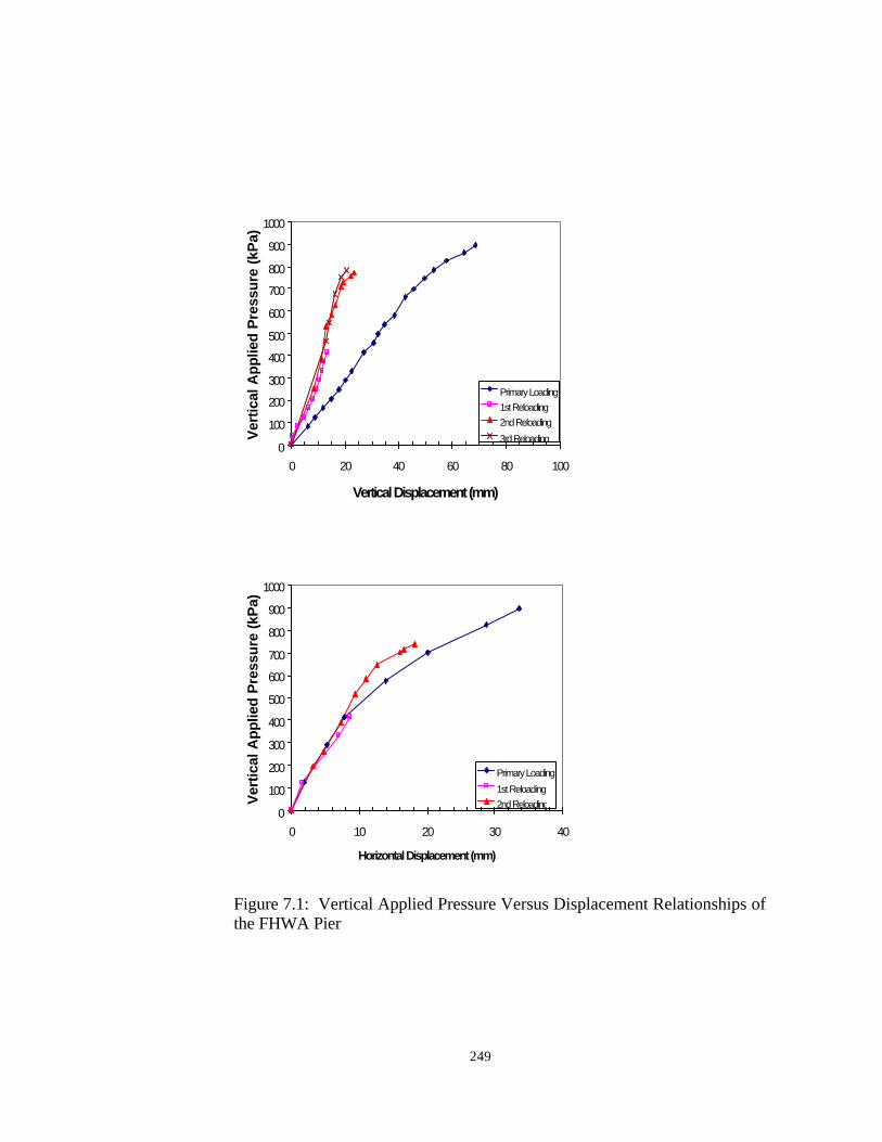
249

Figure 7.1: Vertical Applied Pressure Versus Displacement Relationships of the FHWA Pier

0

100

200

300

400

500

600

700

800

900

1000

0 20 40 60 80 100

Vertical Displacement (mm)

Verti

cal A

pplie

d Pr

essu

re (k

Pa)

Primary Loading1st Reloading2nd Reloading3rd Reloading

0

100

200

300

400

500

600

700

800

900

1000

0 10 20 30 40

Horizontal Displacement (mm)

Verti

cal A

pplie

d Pr

essu

re (k

Pa)

Primary Loading1st Reloading2nd Reloading

250

Figure 7.2: Vertical Load Versus Displacement Relationships of the SPG Test

0

50

100

150

200

250

300

350

400

450

0 5 10 15 20 25

Vertical Displacement (mm)

Vert

ical

Loa

d (k

N)

Primary LoadingReloading

0

50

100

150

200

250

300

350

400

450

0 2 4 6 8 10 12

Horizontal Displacement (mm)

Vert

ical

Loa

d (k

N)

Primary LoadingReloading

251

Figure 7.3: Vertical Improvement Ratio Versus Applied Load Level Relationships of the FHWA Pier and SGP Test

0

1

2

3

4

5

0.00 0.20 0.40 0.60 0.80 1.00

Applied Load Level

Vert

ical

Impr

ovem

ent R

atio

FHWA PierSGP Test

252

Figure 7.4: Horizontal Improvement Ratio Versus Applied Load Level Relationships of the FHWA Pier and SGP Test

0

1

2

3

4

5

0.00 0.20 0.40 0.60 0.80 1.00

Applied Load Level

Hor

izon

tal I

mpr

ovem

ent R

atio

FHWA PierSGP Test

253

7.2 Black Hawk Abutments The project description of the Black Hawk abutments was given in Chapter 2.

Differing from the FHWA pier, the Black Hawk abutments were a production project. The abutments were preloaded to reduce anticipated differential post-construction settlement due to largely different thickness of the GRS masses. The abutments were preloaded in October 1997. The loading sequence consisted of primary loading and three cycles of reloading. During primary loading, increasing vertical loads were incrementally applied up to 245 kPa (1.6 times the design load of 150 kPa) and then unloaded to zero. Three loading-unloading cycles were applied following the primary loading. In the reloading cycles, the applied pressure was approximately the design load of 150 kPa.

7.2.1 Full-Scale Preloading Results

Figures 7.5 and 7.6 show vertical applied pressure versus average settlement relationships of Footings #1 and #3 (for footing descriptions, see Section 2.4.1.4). The average settlement was calculated from the settlements at four corners of each footing. The vertical load-settlement behavior of the footings shows the effect of preloading in reducing footing settlement. At 150 kPa, the average settlements of Footings #1 and #3 were, respectively, 13.3 mm and 28.0 mm. At the same vertical pressure, the average settlements of Footings #1 and #3 reduced to, respectively, 2.8 mm and 4.2 mm. The differences of the settlements between Footing #1 and Footing #3 were due to different thickness of the GRS masses and different boundary conditions (where the footing was positioned with respect to the rock-faced wall). Figures 7.5 and 7.6 also show that the settlements in all the reloading paths were comparable and much smaller than the settlement in the primary loading. This indicates that the preloading effect is insignificant in subsequent reloading paths. This behavior was also observed in the FHWA pier and the SGP tests.

7.2.2 SGP Test Results A series of the modified SGP tests were conducted on the Road Base soil with Amoco 2044 reinforcement. The test results were presented in Chapter 5. Figure 7.7 shows the vertical load versus vertical displacement relationships of the SGP tests (Tests P-M-(RB+2044) and P-UR-(RB+2044)). The predicted values from the SPR model described in Chapter 6 are also included. Both the measured and predicted displacements showed the effect of preloading in reducing the vertical displacements. 7.2.3 Correlation Between the Modified SGP Test and Black Hawk Abutments The correlation between the modified SGP tests and the Black Hawk abutments is presented. The ultimate load of the footing was determined by assuming

254

a hyperbolic relationship between the vertical pressure and the average settlement. The ultimate loads of Footings #1 and #3 were 370 kN and 330 kN, respectively. The vertical improvement ratios of the footings were compared with those from the SGP tests and the SPR model, as shown in Figure 7.8. The VIR values from the SGP test and the SPR model were smaller than the measured data. At an applied load level of 0.25, the VIF values from the SGP tests and the SPR model were 2.3 and 1.8, respectively; whereas, the measured data of Footings #1 and #3 showed that the VIR values were about 3.6.

The large discrepancy in the VIR values is attributed to the difference in the placement density. In the FHWA pier, the field density was closely monitored by field density tests to ensure uniformity. The field density of the Black Hawk abutments was controlled by experience without field density measurement. As a result, the field density was not as well controlled and not as uniform as the FHWA pier. The field density was most likely lower than in the SGP test (95% R.C. Standard Proctor). The lower density led to a large compression of the backfill during preloading, hence, higher VIR values.

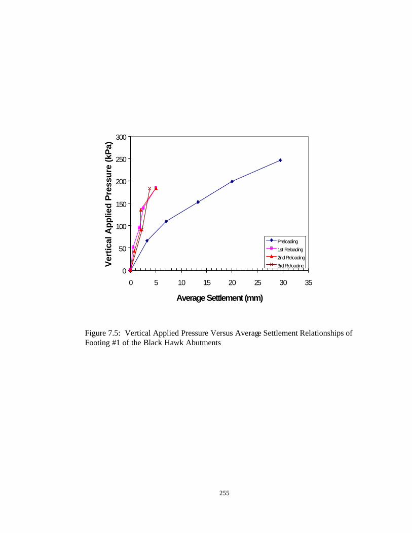
255

Figure 7.5: Vertical Applied Pressure Versus Average Settlement Relationships of Footing #1 of the Black Hawk Abutments

0

50

100

150

200

250

300

0 5 10 15 20 25 30 35

Average Settlement (mm)

Verti

cal A

pplie

d Pr

essu

re (k

Pa)

Preloading1st Reloading2nd Reloading3rd Reloading

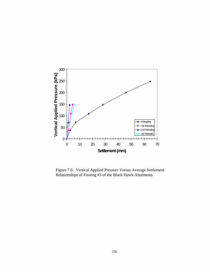
256

Figure 7.6: Vertical Applied Pressure Versus Average Settlement Relationships of Footing #3 of the Black Hawk Abutments

0

50

100

150

200

250

300

0 10 20 30 40 50 60 70

Settlement (mm)

Verti

cal A

pplie

d Pr

essu

re (k

Pa)

Preloading1st Reloading2nd Reloading3rd Reloading

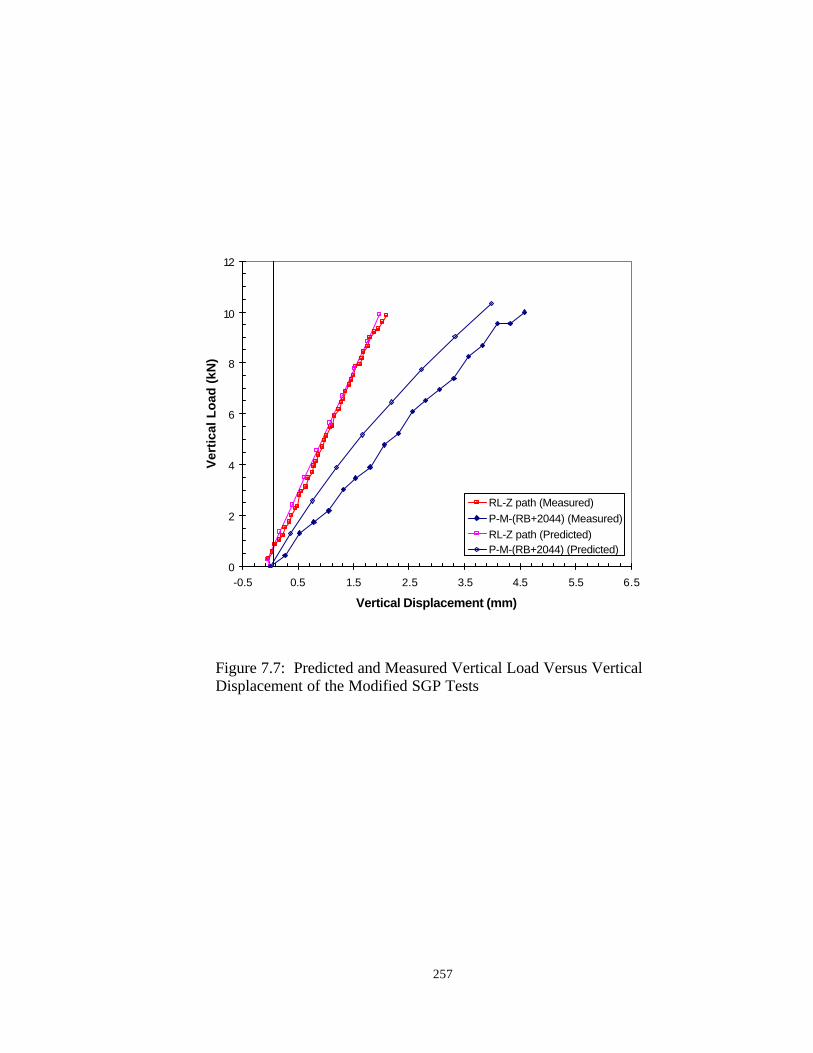
257

Figure 7.7: Predicted and Measured Vertical Load Versus Vertical Displacement of the Modified SGP Tests

0

2

4

6

8

10

12

-0.5 0.5 1.5 2.5 3.5 4.5 5.5 6.5

Vertical Displacement (mm)

Vert

ical

Loa

d (k

N)

RL-Z path (Measured)P-M-(RB+2044) (Measured)RL-Z path (Predicted)P-M-(RB+2044) (Predicted)

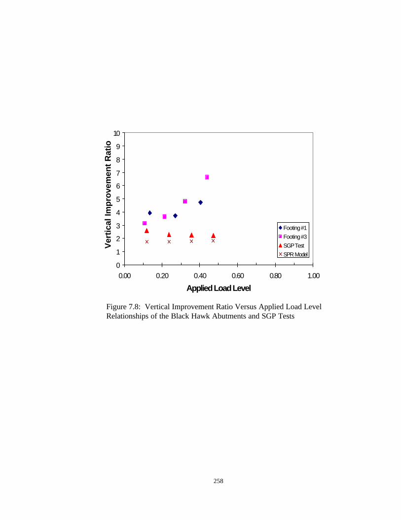
258

Figure 7.8: Vertical Improvement Ratio Versus Applied Load Level Relationships of the Black Hawk Abutments and SGP Tests

0

1

2

3

4

5

6

7

8

9

10

0.00 0.20 0.40 0.60 0.80 1.00

Applied Load Level

Vert

ical

Impr

ovem

ent R

atio

Footing #1Footing #3SGP TestSPR Model

259

7.3 Summary and Concluding Remarks The vertical and horizontal improvement ratios (VIR and HIR) from the SGP

test correlated quite well with those of the FHWA pier despite the large differences in geometry and boundary conditions between them. The difference in VIR and HIR between the SGP test and the FHWA pier was within 10%. In the Black Hawk abutments, the SGP tests and the SPR model give about 40% lower VIR values than the VIR from the measured data. The difference is believed to be due to the uncertainty in the placement density and moisture of the backfill in the abutments.

The degree of reduction in the settlement due to preloading of GRS structures may be assessed with reasonable accuracy by conducting a SGP test or simply using the SPR model. Additional validation is still needed as more reliable field-measured data of preloaded GRS structures become available.

260

8. Summary, Conclusions, and Recommendations 8.1 Summary A study was undertaken to investigate the behavior of a geosynthetic-reinforced soil (GRS ) mass subject to preloading and to develop a simplified analytical model for estimating deformation of a preloaded GRS mass. Since 1997, preloading has been applied to a number of full-scale GRS structures. The preloading has been shown to reduce settlements in the subsequent loading paths. However, the behavior of a preloaded GRS mass has not yet been fully elucidated. Specifically, two important questions remain unanswered: 1. What is the appropriate loading magnitude and loading sequence to effectively

preload a GRS mass? 2. How much deformation is to be expected in a preloaded GRS mass? To seek answers to these questions, a systematic study was conducted. Specifically, the following four tasks were carried out: Task 1: Conduct laboratory tests to examine the behavior of different soils, geosynthetics, and soil-geosynthetic interfaces subject to monotonic loading and unloading-reloading. The test programs included conventional triaxial tests on soils, in- isolation load-extension tests on geosynthetics, and direct shear tests on soil-geosynthetic interfaces. The soils were an Ottawa sand and a Road Base soil. The Road Base soil was a granular material commonly used as backfill for GRS structures. The geosynthetics were a woven polypropylene geotextile, Amoco 2044, as a strong reinforcement and a non-woven heat-bonded polypropylene geotextile, Typar 3301, as a weak reinforcement. Task 2: Conduct laboratory tests to examine the behavior of generic GRS masses subject to monotonic loading and unloading-reloading. The tests were conducted by a modified soil-geosynthetic performance (SGP) test devised in this study. Vertical and horizontal deformations of the test specimen were measured. In one test, strain gauges were installed to measure strains in the reinforcement. A finite element analysis was conducted to examine the stress distribution of a GRS mass in the SGP test under monotonic loading. Task 3: Develop a simplified analytical model, referred to as the simplified preloading-reloading (SPR) model, for estimating deformation of a preloaded GRS mass. The SPR model consists of two principal modules: a load-transfer module and a deformation module. The load-transfer module is based on the elastic analysis of an idealized plane-strain GRS mass. The load-transfer module can be used to calculate the average stresses in a GRS mass. The deformation module can be used to calculate the vertical and horizontal deformations of a GRS mass based on the average stresses from the load-transfer module. The SPR model was verified by the results of experimental tests and numerical analysis of the APSR test and by the results of the SGP tests conducted in this study.

261

Task 4: Examine the correlations between the SGP test and preloaded GRS structures. The correlations were made with normalized loads and normalized displacements, referred to as the vertical and horizontal improvement factors (VIR and HIR). Two full-scale GRS structures, the FHWA pier and the Black Hawk abutments, and corresponding SGP tests were used to examine the correlations. 8.2 Findings and Conclusions The findings and conclusions of this study are organized into four groups, namely: (1) laboratory tests of soils, geosynthetics, and interfaces, (2) SGP tests and finite element analysis, (3) the simplified preloading-reloading (SPR) model, and (4) correlations between SGP test and preloaded GRS structures. (1) Laboratory Tests of Soils, Geosynthetics, and Interfaces 1. The stiffness of the soils increased as a result of preloading. The reloading

stiffness was found to depend on the confining pressure and the unloading load level. At the same confining pressure, the reloading stiffness of the RL-PS path was higher than in the RL-Z path. The RL-Z path was a reloading path that initiated from a zero- load level, whereas the RL-PS path was a reloading path that initiated from a prestressed load level.

2. The stiffness of the preloaded geosynthetic specimen was higher than that of the corresponding virgin specimen, provided that the preloading load level was less than about 50% of the ultimate tensile strength. The reloading stiffness reduced with increasing preloading load level.

3. The reloading stiffness of the preloaded interface was higher than that of the interface without preloading. The reloading stiffness of the interface increased with normal stress applied on the interface.

4. The preloading did not affect the shear strength of the soils or the interfaces. 5. The tensile strength of the preloaded geosynthetic specimen was only about 5%

lower than that of the corresponding virgin specimen. (2) SGP Tests and Finite Element Analysis (A) Monotonic-Loading SGP Tests 1. Due to the reinforcing effects imposed by the reinforcement, a soil mass with

reinforcement had higher stiffness and strength than without reinforcement. The stiffness of the soil mass with reinforcement was about 30% higher than without reinforcement.

2. Some vertical and horizontal deformations were required to mobilize the reinforcing effects. Before the reinforcing effect was fully mobilized, the soil mass with and without reinforcement showed comparable deformations. For the Road Base soil mass with or without reinforcement, the required vertical and horizontal displacements to fully mobilize the reinforcing effect were 2.0 mm and 0.5 mm, respectively.

262

(B) Unloading-Reloading SGP Tests 1. With preloading, the stiffness of the GRS mass increased significantly. For the

GRS mass comprising the Ottawa sand and Amoco 2044 geotextile reinforcement, the stiffness increased by factors of 3 to 7 in the vertical direction, and about 7 in the horizontal direction. For the GRS mass comprising the Road Base soil and Amoco 2044 geotextile reinforcement, the stiffness increased by factors of 2 to 5 in the vertical direction, and about 3 in the horizontal direction.

2. The magnitude of the preloading load level did not appear to affect the reloading stiffness except at the initial stage of the reloading path. During the initial stage of the reloading path, the rebounding deformation continued if the test specimen was unloaded from a high preloading load level to a zero- load level. Similar rebounding deformation behavior was also observed in the FHWA pier after unloading had completed.

3. The RL-PS path showed higher vertical reloading stiffness than the RL-Z path. The vertical reloading stiffness increased with increasing prestressed load level. In the horizontal direction, the RL-Z and RL-PS paths showed comparable horizontal reloading stiffness.

4. The unloading and reloading curves of the multiple unloading-reloading at working load levels nearly coincided with one another. This behavior was also observed in the FHWA pier and the Black Hawk abutments.

5. The reinforcing effect was insignificant during the reloading path. 6. Preloading did not appear to affect the load carrying capacity of the GRS mass. (C) Finite Element Analysis 1. The presence of the reinforcement layers in the soil mass altered the horizontal

and shear stress distributions but not the vertical stress distribution. 2. The horizontal and shear stresses increased significantly near the reinforcement

and resulted in an increase of the minor principal stress. With the increasing minor principal stress, the deformation stiffness and shear strength of the soil were subsequently increased. The reinforcing effect, as quantified by the increase of the minor principal stress, was largest near the reinforcement and reduced with the increasing distance from the reinforcement.

(3) Simplified Preloading-Reloading (SPR) Model 1. The SPR model is capable of predicting experimental and numerical analysis

results of the APSR test and the SGP test conducted in this study. Although further verification is still needed, the SPR model appears to be a simple and valid tool for estimating the deformation of GRS masses.

2. The parametric study carried out by the SPR model showed that the vertical displacement of the GRS mass was significantly reduced by increasing the soil stiffness. The effect of increasing the reinforcement stiffness was much smaller, whereas the effect of the interface stiffness was negligible. This finding supports

263

the benefits of employing a preloading technique in reducing post-construction settlement of GRS structures.

(4) Correlations Between SGP Test and Preloaded GRS Structures 1. The vertical and horizontal improvement ratios (VIR and HIR) from the SGP test

correlated quite well with those of the FHWA pier despite the large differences in the geometry and boundary conditions between them. The difference in VIR and HIR from the SGP test and the FHWA pier was within 10%. In the Black Hawk abutments, the SGP tests and the SPR model gave about 40% lower VIR values than the VIR from the measured data. The difference is believed to be due to the uncertainty in the placement density and moisture of the backfill in the abutments.

2. The degree of reduction in the settlement due to preloading of GRS structures may be assessed with reasonable accuracy by conducting a SGP test or simply using the SPR model. Additional validation is still needed as more reliable field- measured data of preloaded GRS structures become available.

8.3 Recommendations 1. Effects of preloading on creep deformation of GRS structures should be

investigated. Accelerated creep tests of a generic GRS mass can be conducted by the SGP test in an elevated temperature incubator, as demonstrated by Ketchart and Wu (1996). It was observed in the FHWA pier that preloading reduced the creep deformation in the subsequent loading paths (Adams, 1997). Tatsuoka et al. (1997) also reported the reduction of creep deformation in the full-scale test of preloaded GRS walls. A systematic study on creep deformation is needed.

2. The SPR model should be further evaluated with different types of soils and geosynthetics. The strain-rate dependent properties of some geosynthetics and the soil model that can account for creep and stress- induced anisotropy may be incorporated in the SPR model.

264

References

Abramento, M. (1993) “Analyses and Measurement of Stresses in Planar Soil Reinforcements,” Thesis submitted to Massachusetts Institute of Technology, in partial fulfillment of the requirements for the degree of Doctor of Philosophy.

Abramento, M. and Whittle, A.J. (1993) “Shear-Lag Analysis of Planar Soil Reinforcement in Plane-Strain Compression,” J. of Engineering Mechanics, ASCE, Vol. 119, No. 2, pp. 270-291.

Adams, M.T. (1997) “Performance of a Prestrained Geosynthetic-Reinforced Soil Bridge Pier,” Int. Sym. On Mechanically Stabilized Backfill, Wu, J.T.H. (ed), Denver, USA, Balkema, pp. 35-53.

Adams, M.T. (1999) Personal communication. Adib, M.E. (1988) “Internal Lateral Pressures in Earth Walls,” Thesis

submitted to University of California at Berkeley, in partial fulfillment of the requirements for the degree of Doctor of Philosophy.

Arthur, J.R.F., Chua, K.S., and Dunstan, T. (1977) “Induced Anisotropy in a Sand,” Geotechnique, Vol. 27, No. 1, pp. 13-30. ASTM D 2850 “Standard Test Method for Unconsolidated, Undrained Compressive Strength of Cohesive Soils,” American Society for Testing and Materials, Philadelphia, PA, USA.

ASTM D 3080 “Standard Test Method for Direct Shear Test of Soils under Consolidated Drained Conditions,” American Society for Testing and Materials, Philadelphia, PA, USA.

ASTM D 4595 “Standard Test Method for Tensile Properties of Geotextiles by the Wide-Width Strip Method,” American Society for Testing and Materials, Philadelphia, PA, USA.

ASTM D 698 “Standard Test Method for Mositure-Density Relations of Soils and Soil-Aggregate Mixtures Using 5.5- lb Rammer and 12- in. Drop,” American Society for Testing and Materials, Philadelphia, PA, USA.

Barden, L., Ismail, H., and Tong, P. (1969) “Plane Strain Deformation of Granular Material at Low and High Pressures,” Geotechnique, Vol. 19, No. 4, pp. 441-452.

Bathurst, R.J. and Cai, Z. (1994) “In-Isolation Cyclic Load-Extension Behavior of Two Geogrids,” Geosynthetic International, Vol. 1, No. 1, pp. 1-9.

Billiard , J.W. and Wu, J.T.H. (1991) “Load Test of a Large-Scale Geotextile-Reinforced Retaining Wall,” Geosynthetics’91, Atlanta, Georgia, pp. 537-548.

Bishop, A.W. and Eldin, A.K.G. (1953) “The Effect of Stress History on the Relation Between φ and Porosity in Sand,” Proc. 3rd Int. Conf. on Soil Mech. and Foundation Engrg., Vol. 1, pp. 100-105.

Boulanger, R.W., Bray, J.D., Chew, S.H., Seed, R.B., Mitchell, J.K., and Duncan, J.M. (1991) “SSCOMPPC: A Finite Element Analysis Program for

265

Evaluation of Soil-Structure Interaction and Compaction Effects PC Version 1.0,” Geotechnical Engineering Report No. UCB/GT/91-02, University of California at Berkeley.

Boyle, S.R. (1995) “Unit Cell Tests on Reinforced Cohesionless Soils,” Proc. Geosynthetic’95, pp. 1221-1234.

Broms, B. (1978) “Triaxial Tests with Fabric-Reinforced Soil,” Proc. Int. Conf. on Use of Fabrics in Geotechnics, L’Ecole Nationale des Ponts et Chaussees, Vol. 3, Paris, France, pp. 129-133.

Butterfield, R., Harkness, R.M., and Andrawes, K.Z. (1970), “A Stereo-Photogrammetric Method for Measuring Displacement Fields,” Geotechnique, Vol. 20, No. 3, pp. 308-314.

Chou, N.N.S. and Wu, J.T.H. (1993) “Investigating Performance of Geosynthetic-Reinforced Soil Walls,” Report No. CDOT-UCD-93-21, Colorado Dept. of Transportation, 341p.

Clough, G.W. and Duncan, J.M. (1969) “Finite Element Analyses of Port Allen and Old River Locks,” Geotechnical Engineering Report No. TE-69-3, University of California at Berkeley.

Collin, J.G. (1986) “Earth Wall Design,” Thesis submitted to University of California at Berkeley, in partial fulfillment of the requirements for the degree of Doctor of Philosophy.

Coon, M.D. and Evans, R.J. (1971) “Recoverable Deformation of Cohesionless Soils,” J. of Geotech. Engrg. Div., Vol. 97, SM. 2, pp. 375-391.

Dong, J., Nakamura, K., Tatsuoka, F., and Kohata, Y. (1994) “Deformation Characteristics of Gravels in Triaxial Compression Tests and Cyclic Triaxial Tests,” Int. Sym. On Pre-Failure Deformation Characteristics of Geomaterials, IS Hokkaido’94, Vol. 1, pp. 17-23.

Duncan, J.M. (1994) “The Role of Advanced Constitutive Relations in Practical Applications,” Proc. 13th Int. Conf. on Soil Mech. and Foundation Engrg., pp. 31-48.

Duncan, J.M. and Chang, C.Y. (1970) “Nonlinear Analysis of Stress and Strain in Soils,” J. of Geotech. Engrg. Div., Vol. 96, SM. 5, pp. 1629-1653.

Duncan, J.M. and Chang, C.Y. (1972) closure to “Nonlinear Analysis of Stress and Strain in Soils,” J. of Geotech. Engrg. Div., Vol. 98, SM. 5, pp. 495-498.

Duncan, J.M., Byrne, P., Wong, K.S., and Mabry, P. (1980) “Strength, Stress-Strain and Bulk Modulus Parameters for Finite Element Analysis of Stress and Movements in Soil Masses,” Geotechnical Engineering Report No. UCB/GT/80-01, University of California at Berkeley.

Elias, V. and Christopher, B. (1996) “Mechanically Stabilized Earth Walls and Reinforced Soil Slopes: Design and Construction Guideline,” Publication No. FHWA-SA-96-071, FHWA, US Dept. of Transportation.

266

Goodman, R.E., Taylor, R.L., and Brekke, T.L. (1968) “A Model for the Mechanics of Jointed Rock,” J. of Geotech. Engrg. Div., Vol. 94, SM. 4, pp. 637-659.

Goto, S., Tatsuoka, F., Shibuya, S., Kim, Y.-S., and Sato, T. (1991) “A Simple Gauge for Local Small Strain Measurements in the Laboratory,” Soils and Foundations, Vol. 31, No. 1, pp. 169-180.

Gray, D. and Al-Rafeai, T. (1986) “Behavior of Fabric- Versus Fiber-Reinforced Sand," J. of Geotech. Engrg. Div., Vol. 112, No. 8, pp. 804-820.

Gray, D.H. and Al-Refeai, T. (1986) “Behavior of Fabric- versus Fiber-Reinforced Sand,” J. of Geotech. Engrg. Div., Vol. 112, No. 8

Hermann, L.R. and Al-Yassin, Z. (1978) “Numerical Analysis of Reinforced Soil Systems,” ASCE Proc. Sym. On Earth Reinforcement, Pittsburg, PA, pp. 428-457.

Holtz, R.D., Tobin, W.R., and Burke, W.W. (1982) “Creep Characteristics and Stress-Strain Behavior of a Geotextile-Reinforced Sand,” Proc. of the Second Int. Conf. On Geosynthetics, Las Vegas.

Holubec, I. (1968) “Elastic Behavior of Cohesionless Soil,” J. of Geotech. Engrg. Div., Vol. 94, SM. 6, pp. 1215-1231.

Hoque, E., Tatsuoka, F., Sato, T., and Kohata, Y. (1995) “Inherent and Stress-Induced Anisotropy in Small-Strain Stiffness of Granular Materials,” Proc. 1st. Int. Conf. of Earthquake Geotechnical Engineering, IS Tokyo’95, Vol. 1, pp. 277-282.

Hyodo, M., Yamamoto, Y., and Sugiyama, M. (1994) “Undrained Cyclic Shear Behaviour of Normally Consolidated Clay subjected to Initial Static Shear Stress,” Soils and Foundations, Vol. 34, No. 4, pp. 1-11.

Ishihara, K. (1996) “Soil Behavior in Earthquake Goetechnics,” Oxford University Press Inc., New York, 350p.

Jaber, M (1989) “Behavior of Reinforced Soil Walls in Centrifuge Model Tests,” Thesis submitted to University of California at Berkeley in partial fulfillment of the requirements for the degree of Doctor of Philosophy.

Jaber, M. (1990) “Behavior of Reinforced Soil Walls in Centrifuge Model Tests,” Thesis submitted to University of California at Berkeley, in partial fulfillment of the requirements for the degree of Doctor of Philosophy.

Jewell, R.A. (1993) “Links between the Testing, Modelling, and Design of Reinforced Soil,” Proc. Int. Symp. Earth Reinforcement Practice, Fukuoka, Japan, Balkema, pp. 755-772.

Jewell, R.A. and Wroth, C.P. (1987) “Direct Shear Tests and Reinforced Sand,” Geotechnique, Vol. 37, No. 1, pp. 53-68.

Ketchart, K. and Wu, J.T.H. (1996) " Long-Term Performance Tests of Soil-Geosynthetic Composites," Technical Publication No. CDOT-CTI-96-1, Colorado Department of Transportation, 156 p.

267

Klosky, J.L. (1997) “Behavior of Composite Granular Materials and Vibratory Helical Anchors,” Thesis submitted to University of Colorado at Boulder, in partial fulfillment of the requirements for the degree of Doctor of Philosophy.

Ko, H.Y. and Scott, R.F. (1967) “Deformation of Sand in Shear,” J. of Geotech. Engrg. Div., Vol. 93, SM. 5, pp. 283-310.

Ko, H.-Y. and Sture, S. (1981) “State of the Art: Data Reduction and Application for Analytical Modeling,” Conf. on Laboratory Shear Strength, ASTM STP 740, pp. 229-386.

Ko, H.-Y. and Sture, S. (1981) “State of the Art: Data Reduction and Application for Analytical Modeling,” Laboratory Shear Strength of Soil. ASTM STP 740, pp. 329-386.

Kondner, R.L. (1963) “Hyperbolic Stress-Strain Response: Cohesive Soil,” J. of Geotech. Engrg. Div., Vol. 89, SM. 1, pp. 115-143.

Ladd, R.S. (1977) “Stress-Deformation and Strength Characteristics: State-of-the-Art Report,” Proc. 9th Int. Conf. on Soil Mech. and Foundation Engrg., Vol. 2

Lade, P.V. and Duncan, J.M. (1975) “Elastoplastic Stress-Strain Theory for Cohesionless Soil,” J. of Geotech. Engrg. Div., Vol.101, GT. 10, pp. 1037-1053.

Lade, P.V. and Duncan, J.M. (1976) “Stress-Path Dependent Behavior of Cohesionless Soil,” J. of Geotech. Engrg. Div., Vol. 102, GT. 1, pp. 51-68.

Lambrechts, J.R. and Leonards, G.A. (1978) “Effects of Stress History on Deformation of Sand,” J. of Geotech. Engrg. Div., Vol.104, GT.11, pp.1371-1387.

Larson, D.G. (1992) “A Laboratory Investigation of Load-Transfer in Reinforced Soil,” Thesis submitted to Massachusetts Institute of Technology, in partial fulfillment of the requirements for the degree of Doctor of Philosophy.

Ling, H.I. and Tatsuoka, F. (1992) “Nonlinear Analysis of Reinforced Soil Structures by Modified CANDE (M-CANDE),” Proc. of Int. Sym. On Geosynthetic-Reinforced Soil Retaining Walls, Denver, Colorado, pp. 279-291.

Ling, H.I. and Tatsuoka, F. (1993) “Performance of Anisotropic Geosynthetic-Reinforced Cohesive Soil Mass,” J. of Geotech. Engrg. Div., Vol. 120, No. 7, pp. 1166-1184.

Lubahn, J.D. and Felgar, R.P. (1961) “Plasticity and Creep of Metals,” Wiley, New York.

Makhlouf, H.M. and Stewart, J.J. (1965) “Factors Influencing the Modulus of Elasticity of Dry Sand,” Proc. 6th Int. Conf. on Soil Mech. and Foundation Engrg., Vol. 1, pp. 298-302.

Martin, J.P., Koerner, R.M., and Whitty, J.E. (1984) “Experimental Friction Evaluation of Slippage between Geomembranes, Geotextiles, and Soils,” Proc. Int. Conf. on Geomembranes, Industrial Fabrics Association International, pp. 191-196.

McGown, A., Andrewes, K.Z., and Al-Hasani, M.M. (1978) “Effect of Inclusion Properties on the Behavior of Sand,” Geotechnique, Vol. 28, No. 3, pp. 327-346.

268

Mendelson, A. (1968) “Plasticity: Theory and Applications,” Macmillan, New York.

Moraci, N., and Montanelli, F. (1997) “Behavior of Geogrids Under Cyclic Loads,” Proc., Geosynthetic ’97 Conf., pp. 961-976.

Mould, J.C. (1983) “Stress Induced Anisotropy in Sand and the Evaluation of Multi-Surface Elasto-Plastic Material Model,” Thesis submitted to University of Colorado at Boulder, in partial fulfillment of the requirements for the degree of Doctor of Philosophy.

Mould, J.C., Sture, S., and Ko, H.-Y. (1982) “Modeling of Elastic-Plastic Anisotropic Hardening and Rotating Principal Stress Directions in Sand,” Proc. IUTAM Conf. Deformation and Failure of Granular Materials, Delft, The Netherlands, pp. 431-439.

Mroz, Z. (1967) “On the Description of Anisotropic Work Hardening,” J. Mech. Phys. Sci., Vol. 15, pp. 163-175.

Nicola, M. and Filippo, M. (1997) “Behavior of Geogrids Under Cyclic Loads,” Proc. Geosynthetic’97, Long Beach, CA, pp. 961-976.

O’Rourke, T.D., Druschel, S.J., and Netravali, A.N. (1990) “Shear Strength Characteristics of Sand-Polymer Interfaces,” J. of Geotech. Engrg. Div., Vol. 116, No. 3, pp. 451-469.

Palmeira, E.M. (1988) Discussion of “Direct Shear Tests and Reinforced Sand,” by R.A. Jewell and C.P. Wroth, Geotechnique, Vol. 38, No. 1, pp. 146-148.

Perkins, S.W. (1991) “Modeling of Regolith Structure Interaction in Extraterrestrial Constructed Facilities,” Thesis submitted to University of Colorado at Boulder, in partial fulfillment of the requirements for the degree of Doctor of Philosophy.

Perriello-Zampelli (1983) “Behavior of Granular Cohesionless Soils at Very Low Effective Stress Levels,” thesis submitted to University of Colorado at Boulder, in partial fulfillment of the requirements for the Master degree.

Provost, J.H. (1981) “Nonlinear Anisotropic Stress-Strain-Strength Behavior of Soils,” Conf. on Laboratory Shear Strength, ASTM STP 740, pp. 431-455.

Sawicki, A. (1998) “Modeling of Geosynthetic Reinforcement in Soil Retaining Walls,” Geosynthetic International, Vol. 5, No. 3, pp. 327-345.

Saxena, S.K. and Wong, Y.T. (1984) “Friction Characteristics of a Geomembrane,” Proc. Int. Conf. on Geomembranes, Industrial Fabrics Association International, pp. 187-190.

Seed, R.B. and Duncan, J.M. (1984) “SSCOMP: A Finite Element Analysis Program for Evaluation of Soil-Structure Interaction and Compaction Effects,” Geotechnical Engineering Report No. UCB/GT/84-02, University of California at Berkeley.

269

Smith, G.N. (1977) “Principles of Reinforced Earth Design,” Proc. Sym. On Reinforced Earth and Other Composite Soil Technique, TRRL Supplementary Report 457, Edinburg, pp.2-21.

Tatsuoka and Shibuya (1991) 9th Asian Region Conf. of Soil Mech. And Foundation Eng., Bangkok, Thailand, Vol. 2, pp. 114.

Tatsuoka, F. and Kohata, Y. (1995) “Stiffness of Hard Soils and Soft Rocks in Engineering Applications,” Int. Sym. On Pre-Failure Deformation Characteristics of Geomaterials, IS Hokkaido’94, Vol. 2, pp. 947-1063.

Tatsuoka, F. and Yamauchi, H. (1986) “A Reinforcing Method for Steep Clay Slopes with a Nonwoven Geotextile,” Geotextiles and Geomembranes, Vol. 4, Nos. 3&4, pp. 241-268.

Tatsuoka, F., Molenkamp, F., Torii, T., and Hino, T. (1984) “Behavior of Lubrication Layers of Platens in Element Tests,” Soils and Foundations, Vol. 24, No. 1, pp. 113-128

Tatsuoka, F., Uchimura, T. and Tateyama, M. (1997) “Preloaded and Prestressed Reinforced Soil,” Soils and Foundations, Vol. 37, No. 3, pp. 79-94.

Uchimura, T., Tatsuoka, F., Tateyama, M., and Koga, T. (1998) “Preloaded-Prestressed Geogrid-Reinforced Soil Bridge Pier,” Proc. of the Sixth Int. Conf. on Geosynthetics, Atlanta, GA, pp. 565-572.

Vermeer, P.A. (1996) “Evaluation for Soil Stiffness Parameters,” ASCE Workshop on Computational Geotecnics, U. of Colorado, Section 4.

Whittle, A.J., Germaine, J.T., Larson, D.G., and Abramento, M. (1992) “Measurement and Interpretation of Reinforcement Stresses in the APSR Cell,” Proc. Int. Symp. Earth Reinforcement Practice, Fukuoka, Japan, Balkema, pp. 179-184.

Whittle, A.J., Larson, D.G., and Abramento, M. (1991) “Annual Technical Report on Geosynthetic Reinforcement of Soil Masses,” Research Report, Dept. of Civil Engineering, Massachusetts Institute of Technology.

Williams, N.D. and Houlihan, M.F. (1987) “Evaluation of Interface Properties between Geosynthetics and Soils,” Proc. Geosynthetics’87, pp. 616-627. Wood, D.M. (1990) “Soil Behavior and Critical State Soil Mechanics,” Cambridge University Press, 425p.

Wu, J.T.H. (1989) “Behavior of Soil-Geotextile Composites and Its Application to Finite Element Analysis,” Proc. Geosynthetics’89, pp. 365-372.

Wu, J.T.H. (1992) “Predicting Performance of the Denver Walls: General Report,” Proc. of Int. Sym. on Geosynthetic-Reinforced Soil Retaining Walls, Denver, Colorado, pp.3-20.

Wu, J.T.H. (1993) “Discussions: Embankments” Proc. Int. Symp. Earth Reinforcement Practice, Fukuoka, Japan, Balkema, pp. 928-929.

Wu, J.T.H. and Helwany, S.M.B. (1996) “A Performance Test for Assessment of Long-Term Creep Behavior of Soil-Geosynthetic Composites,” Geosynthetic International, Vol. 3, No. 1, pp. 107-124.

270

Wu, J.T.H., Ketchart, K., and Adams, M.T. (1999) “GRS Pier and Abutment” Report submitted to Turner-Fairbank Highway Research Center, Federal Highway Administration.

Yamauchi (1988) “Reinforcing Technique Using Clay Backfill and Non-woven Geotextile,” Thesis submitted to University of Tokyo, in partial fulfillment of the requirements for the degree of Doctor of Philosophy (in Japanese).

Yang, Z. (1974) “ Strength and Deformation Characteristics of Reinforced Sand,” Thesis submitted to University of California at Los Angeles, CA, in partial fulfillment of the requirements for the degree of Doctor of Philosophy.

Yoshimi, Y., Kumabara, F., and Tokimatsu, K. (1975) “One-Dimensional Volume Change Characteristics of Sands Under very Low Confining Stresses,” Soils and Foundations, Vol. 15, No. 3, pp. 51-60.