performance driven frequency/voltage planning for multi
TRANSCRIPT

Performance Driven Frequency/Voltage Planning for
Multi-Core Processors with Thermal Constraints
Honors Thesis Submitted by
Michael Aaron Kadin
In partial fulfillment of the
Sc.B in Electrical Engineering
Brown University
4/22/2008

2
Prepared under the Direction of
Professor Sherief Reda, Advisor
Professor Roderic Beresford, Reader
Professor Jennifer Dworak, Reader

3
Table of Contents
Abstract ............................................................................................................................... 4
Chapter 1: Introduction ....................................................................................................... 5
1.1 Multi-core Architectures........................................................................................... 5 1.2 Temperature Constraints and Thermal Management................................................ 6 1.3 Research Overview ................................................................................................... 8
Chapter 2: Previous Work................................................................................................. 12
Chapter 3: Methods and Models ....................................................................................... 14
3.1 Performance-Power-Temperature Tool-chain ........................................................ 14 3.2 Thermal Model........................................................................................................ 18 3.3 Optimization Using Linear Programming .............................................................. 22 3.4 Scaling Trends ........................................................................................................ 27
Chapter 4: Model Validation and Parameter Learning .................................................... 31
4.1 Validating the Linear Frequency/Power Relationship............................................ 31 4.2 Thermal Model Parameter Fitting and Validation .................................................. 33 4.3 Thermal Model Validation with an FPGA.............................................................. 34
Chapter 5: Experiments and Results ................................................................................ 39
5.1 Frequency Planning ................................................................................................ 39 5.2 Process Priorities and Sensitivity Analysis............................................................. 42 5.3 Frequency and Voltage Planning ............................................................................ 45
Chapter 6: Conclusions ..................................................................................................... 49
References......................................................................................................................... 53
4
Abstract
With feature sizes moving into the nanometer regime, clock frequency and
transistor density increases have resulted in elevated chip temperatures. In order to meet
temperature constraints while still exploiting the performance opportunities created by
continued scaling, chip designers have migrated towards multi-core architectures. Multi-
core architectures use moderate clock frequencies with multiple processing units running
multiple threads to exploit Thread-Level Parallelism (TLP). In this work, we propose a
design for a system that performance-optimizes a multi-core system with thermal
constraints. By adjusting core clock frequencies and voltages, on-chip power dissipation
can be controlled in a scheme that maximizes the chip’s physical performance. We
propose a simple model that accurately simulates the effects that changes in clock
frequency and voltage have on both on-chip power and on-chip temperature. Using the
model, we find the optimal operating conditions for several circumstances. Namely, (1)
standard processor performance, where there is no variation in parameters between the
various cores, (2) optimal core performance where there is no constraint for parameter
similarity between cores, and (3) optimal processor performance with thread priorities,
where each core runs a thread of varied importance. We run several experiments across
six different technology nodes to validate the work, assuring that our models and methods
are accurate. Our methods have been shown to increase the physical performance of a
multi-core system by up to 33.4% with minimal hardware overhead and without violating
a steady-state temperature constraint.
5
Chapter 1: Introduction
1.1 Multi-core Architectures
As scaling continues into the nanometer regime, more transistors are being
fabricated on chips of equal size. Along with these increases in transistor density, clock
frequencies are increasing, creating more switching activity. In ideal scaling, supply
voltages are also decreased in order to avoid high power density. However, thermal noise
and process variations have slowed the scaling of supply voltages in today’s deep sub-
micron chips. High supply voltages themselves do not limit frequency increases; in fact,
high supply voltages can facilitate faster switching speeds. However, without ideal
voltage scaling, on-chip power density increases with technology, and higher power
density leads to higher on-chip temperatures. The temperature problem was traditionally
solved by removing the dissipated energy with improvements in packaging technology
and thermal cooling systems. However, these techniques have become economically
infeasible, and do not scale with technology. Thus, new solutions to the “thermal wall”
are needed.
In order to continue to take advantage of performance improvements enabled by
scaling, chip designers have shifted towards multi-core architectures. Rather than
completing a single process more quickly, multi-core architectures have several
independent cores that simultaneously compute separate threads. Since transistor size
continues to shrink, more cores can be added to a chip of the same area. Though the
smaller transistors have the potential to be run at high frequencies, thermal constraints
continue to restrict their operating frequencies. However, since there are several
6
independent processing units, running them at moderate frequencies does still permit
large performance gains. With an ideal amount of thread level parallelism (TLP),
performance can approximately double with each technology generation.
However, a given workload has a fundamental limit on extractable concurrency.
Thus, situations may occur where all of the cores in a multi-core processor may not be in
use. In fact, coding and compiling for TLP is expected to be one of the most difficult
challenges of the multi-core era.
1.2 Temperature Constraints and Thermal Management
High on-chip temperatures can have several negative effects on a processor.
Increases in thermal noise can cause memory bits to unexpectedly flip. In addition,
raised temperatures increase the likelihood that electrons can escape the quantum well
imposed by an OFF transistor. Thus, high temperatures increase sub-threshold leakage
current, increasing overall processor power consumption. Increased temperatures also
increase Elmore delay, decrease the mean time to failure, and can cause physical damage
to the chip. In general, increased on-chip temperatures are detrimental to processor
performance, power, and reliability.
Solutions to the temperature problem have been proposed from several research
areas. For example, Ku et al. attempt to lower temperatures with a static micro-
architectural design technique [1]. By deactivating alternating cache lines rather than
entire cache banks, power is spread more evenly, and temperature is decreased. Tsai and
Kang [2] approach the temperature problem with a placement algorithm designed to
7
spread heat more evenly. Mutyam et al. [3] propose complier optimizations that more
evenly spread heat between functional units. Successful chip/software designs will likely
incorporate a number of these and similar design changes from many different research
fields.
One of the most active fields that deals with the “thermal wall” is dynamic
thermal management (DTM). DTM methods read in the current thermal state of the chip
with temperature sensors or performance counters, and make changes to processor
parameters to adapt to the chip’s current temperature (or temperature gradient). As
mentioned above, high power densities can currently be handled with expensive
packaging solutions. However, DTM methods seek to avoid the need for these expensive
techniques. A processor that utilizes DTM has a package designed (inexpensively) for
the average power dissipation rather than peak dissipation. When the chip processes a
particularly aggressive code section, and the power dissipation becomes too great for the
packaging to successfully remove, temperatures will rise. DTM techniques sense this
temperature change and adjust chip parameters (frequency, voltage, pipeline width, etc)
to compensate. Most DTM techniques impose some form of performance penalty. For
example, decreasing a pipeline’s width will decrease the number of switching transistors,
and thus, the amount of power dissipated. However, the number of instructions a
processor completes per cycle will also decrease, and this will hurt performance.
Research into DTM techniques attempts to maintain temperature constraints, while
minimizing the performance degradation.
As the industry turns towards multi-core processors, many chip-makers are also
looking to a Globally Asynchronous, Locally Synchronous (GALS) architecture. GALS

8
systems have multiple Voltage/Frequency Islands (VFIs) that operate internally on a
synchronous clock network, but communicate with other VFIs via asynchronous means.
A GALS structure, or similar structures in use, allow different VFIs to operate at different
voltages/frequencies.
Research into DTM techniques has leveraged the independence of different VFIs
for thermal advantages. If a high temperature area forms in one VFI, the entire chip need
not be throttled. Instead, an individual VFI’s parameters can be changed, to eliminate the
hot spot, without affecting the performance of other VFIs. Donald and Martonosi [4]
show that using Dynamic Voltage and Frequency Scaling (DVFS) on individual
voltage/frequency independent cores gives significant performance improvements over
chip-wide DVFS. Mukherjee and Memik [5] develop optimal frequencies for a core and
its surrounding cores for recovery during thermal emergencies.
Upcoming chip designs with several independent processing units, or cores, each
with its own voltage and frequency settings (e.g. AMD Quad-Core Phenom Processor
[6]) set the framework for our methods. Currently chip-designers select voltage and
frequency levels to be equal on all of their cores. Our methodology seeks the optimal
frequency setting for each core in a multi-core system that does not necessarily obey that
identical frequency constraint.
1.3 Research Overview
The International Technology Roadmap for Semiconductors (ITRS) shows that
with increases in technology, chip temperature must be capped at 85° C to alleviate the

9
aforementioned concerns. In this work, we propose a method to increase the physical
performance of a multi-core processor under this thermal constraint. For the sake of this
work, physical performance is defined as the performance of a system based solely on
cycles per second. In other words, we seek to increase on-chip clock frequencies. We
treat chip-wide physical performance as the sum of the frequencies of all of the cores.
Architectural changes and other enhancements complement increases in physical
performance to benefit overall processor throughput, but these additional improvements
are outside the scope of this work.
To begin the performance optimization, a series of high-level models must be
constructed. First, we must model the power dissipated by units within the processor
based on operating parameters. In addition, we must model temperature variations that
result from this released power. These modeling objectives are complicated by a myriad
of factors. First, within the chip, heat is transferred in all three dimensions. Thus, power
released by units within the processor can travel out of the chip via the package, or be
transmitted laterally to other units nearby. Thus, the temperature of a section of the die is
not only dependent on the power dissipated in that section, but also on nearby areas’
power. A second modeling complication arises from coupling between power and
temperature. Leakage current increases with increasing temperature. However,
temperature is a power dependant quantity. With increasing power comes increasing
temperature, which in turn increases power more. Therefore, temperature and power are
coupled through Leakage Dependence on Temperature (LDT). Third, cores exhibit
spatial variations in temperature. In other words, power is not uniformly dissipated
across a core; one area within a core may be significantly hotter than another. A fourth
10
complication comes with changes in process parameters at different technology nodes.
Examinations of current technology nodes (65nm) may not be applicable to future nodes
(45nm, 32nm, and beyond). Lastly, these models are complicated by the fact that
different workloads may use different core modules at different rates. This means that
one process may heat one part of the chip a great deal, while another process may be
power intensive in a totally different section of the die. Our modeling and learning
techniques attempt to conquer all of these difficulties.
Once thermal and power models have been set up, we will propose a methodology
for selecting the frequency for each core in a multi-core system that will optimize full
system performance. In addition, we will propose a method for optimizing the physical
performance in a system where processes have different priorities. The models and
methods will be applied to six different technology nodes: 130nm, 90nm, 65nm, 45nm,
32nm, and 22nm. All of these models and methods will be comprehensively tested and
checked for accuracy. The main contributions of this thesis can be summarized as
follows:
• We propose a simple power-thermal model for multi-core systems that
produces accurate temperatures, while maintaining high-level simplicity.
The model incorporates both vertical and horizontal heat transfer and the
leakage dependence on temperature.
• We use the parameters of the power-thermal model to formulate a design
optimization space. An exploration of this space shows the potential
performance improvements in multi-core systems with thermal
constraints.

11
• We propose using the model and optimization techniques during processor
operation with multiple thread priorities. In this scheme, cores will run
threads of varying importance. The operating system can assign the
optimal frequencies to the cores so that critical threads are completed
more quickly without violating temperature constraints.
• The models, methods, and optimizations are all tested on several systems
and core arrangements, at several technology nodes. In addition, the
results are validated using previously confirmed full-scale power and
thermal models. The results show that it is possible to boost the physical
performance of a multi-core processor by up to 33.4% without violating a
thermal constraint. Most importantly, these optimizations can be executed
with minimal hardware/software overhead.
The rest of this thesis is organized as follows. Chapter 2 briefly reviews some previous
work on optimal multi-core voltage/frequency assignment. Chapter 3 elucidates our
models and methods. Chapter 4 details the techniques and results of our model
validation. Chapter 5 explains the experimental results, and Chapter 6 concludes the
work.
12
Chapter 2: Previous Work
There has been much DTM research focusing on methods for recovering from
thermal emergencies [4],[5],[7],[8],[9],[10]. These works, center mostly on what to do
when a chip’s temperature rises above a certain threshold. Our work, on the other hand,
focuses on maximizing performance under a given steady-state temperature constraint.
In other words, we seek to keep temperature at a reasonably constant level by working
with some of the same parameters that are utilized in the emergency DTM techniques.
Even in our steady-state methods, however, temperatures may fluctuate with code
intensity and external factors. Therefore, it is still possible that sections of the chip may
reach emergency temperatures. Our methodology is designed to complement existing
emergency DTM techniques to maximize processor throughput while still assuring that
the chip will never reach dangerous temperatures.
Some work has been conducted along similar lines. Rao et al. used similar power
and thermal models as in our work, to develop system level expressions for number/speed
of active of cores with thermal constraints [11]. The goal in this work is very similar to
our own: a simple method for determining system-level parameters in thermal
management environments. However, their work chooses to ignore horizontal heat
transfer, which was shown in [5] to be of critical importance. According to Rao, a core
with a hotspot will cool just as effectively while surrounded by 6 hot cores, as it would if
cold cache banks surrounded it. Skadron [12] comments that the horizontal heat transfer
path can account for up to 30% of heat transfer. Thus, we seek to improve upon Rao’s
techniques.

13
Murali et al. [13] propose the use of convex optimization methods to solve the
problem of temperature-aware processor frequency assignments. However, their work
does not offer a clear, generic method to calculate the parameters of the convex model,
and they do not report the speedups achieved while using the proposed method in
comparison to traditional frequency assignment. Furthermore, the reported runtime
required to solve their problem formulations takes “less than few hours” which reduces
the method’s utility in their proposed dynamic setting. Solutions to our linear program
can be solved very quickly.
The importance of multiple VFIs has been called into question by Herbert and
Sebastian [14]. Herbert and Sebastian examine the success of three different DVFS
schemes at varying levels of VFI granularity on a multi-core processor. Their
experiments compared the improvements in energy efficiency for different numbers of
VFIs on chip. The results showed that for a 16 core chip the increases in energy
efficiency for having each core be its own VFI were eclipsed by the increases in cost and
complexity. However, the authors only investigated the possibility of improving energy
efficiency. Donald and Martonosi [4] showed, and our work will confirm, that individual
core VFIs will bring huge performance benefits in the context of thermal management,
and not just energy efficiency. These performance improvements will show that there is
a great deal of utility in having an independent voltage/frequency island for each core in a
multi-core processor.
14
Chapter 3: Methods and Models
3.1 Performance-Power-Temperature Tool-chain
In order to accurately model chip temperature from operating parameters, we
must first obtain temperature data based on real chip behavior. There are several
possibilities for obtaining these measurements. One possibility would be to measure the
on-chip temperatures in real silicon. This can be accomplished with an Infra-Red Camera
[15], or with on-chip temperature sensors such as performance counters, ring oscillators,
or thermal diodes [16]. Alternatively, chip temperature data can be obtained in a
simulation environment. In order to allow for a large amount of data to be collected, to
account for scaling trends, and to keep the optimization environment malleable, we
acquire the majority of the temperature data through a simulator chain. We also validate
our model on a small data set in silicon to assure that the model accurately reflects real
chip behavior.
The temperature gradient of a chip is related to amount of power dissipated on
that chip. Before we can model on-chip temperature, we must first understand where
power is dissipated across the die, and how much power is dissipated. Each core
dissipates its own power, and each core is sub-divided into individual functional units
(ALUs, L1 caches, branch predictors, etc). The power dissipated by each functional unit
is governed by
2dd dd leakP CV f V Iα= + (1)
15
where α is the average switching frequency for all the transistors in the unit, C is the
total capacitance of the gates in the unit, ddV is the supply voltage of the unit, f is the
frequency of the core that the unit is contained within, and leakI is the total leakage current
of the unit. For this work, we chose not to change any architectural parameters; we focus
exclusively on the physical parameters: voltage and frequency. Architectural, system,
and software level optimizations complement our work to maximize total processor
throughput.
Because of the introduction of high-k dielectrics, the effects of gate leakage will
be dominated by sub-threshold leakage current in the coming technology generations.
Therefore, our models only examine sub-threshold leakage current. Sub-threshold
current, is composed of electrons that escape OFF transistor energy wells. Leakage
dependence on temperature (LDT) creates a feedback loop between leakage power and
temperature. Dissipated leakage power increases power density, which in turn increases
temperature. This temperature increase causes further increases in leakage current, which
further increases temperature, and so on. At reasonable temperatures, LDT eventually
converges to a stable value. However, as temperatures increase, the possibility of
“thermal runaway” emerges. At these extreme temperatures, the exponential nature of
LDT cause power to increase until the circuit is permanently damaged.
Therefore, according to (1), in order to calculate the power dissipated for a given
functional unit, we must have accurate measures of the switching constant α , the unit’s
total capacitance C , the voltage and frequency of the core containing the unit, the
leakage current in the unit leakI , and the unit’s temperature so as to accurately model
LDT. The flow in Fig. 1 below was used for this calculation.
16
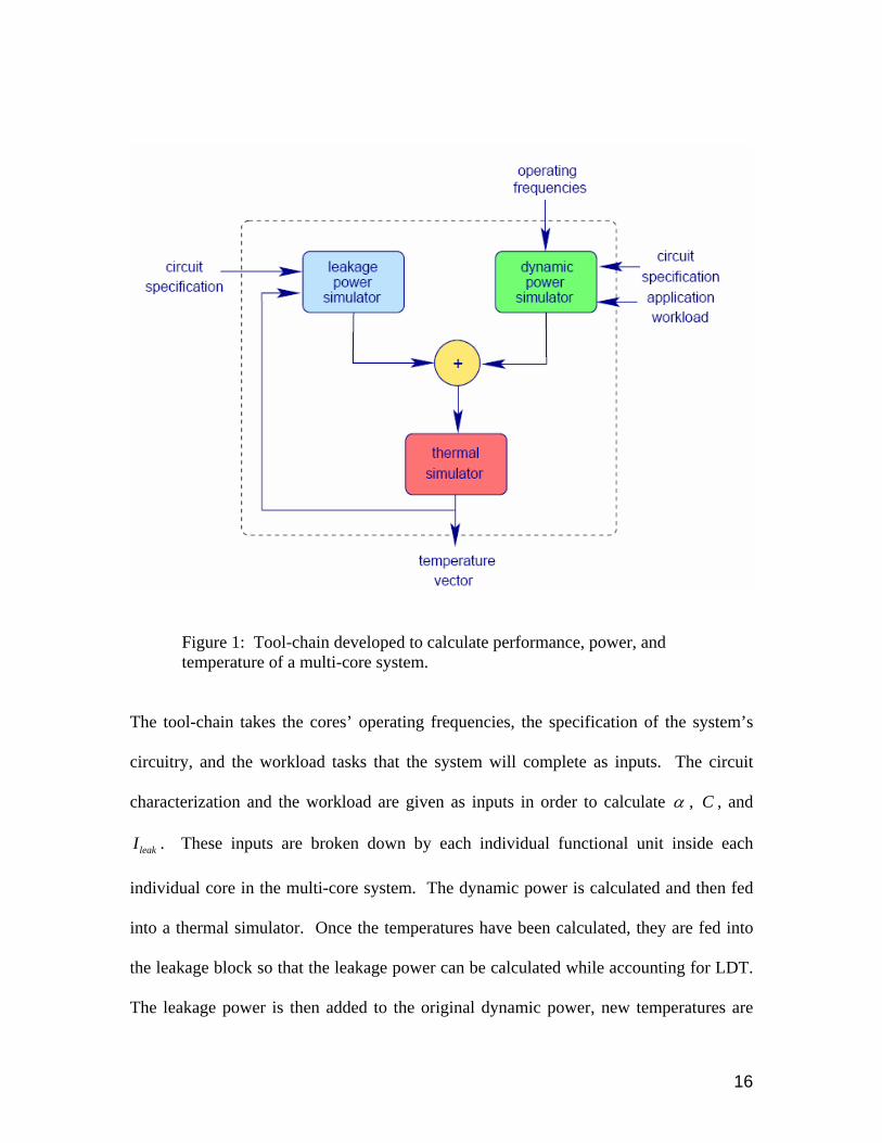
Figure 1: Tool-chain developed to calculate performance, power, and temperature of a multi-core system.
The tool-chain takes the cores’ operating frequencies, the specification of the system’s
circuitry, and the workload tasks that the system will complete as inputs. The circuit
characterization and the workload are given as inputs in order to calculate α , C , and
leakI . These inputs are broken down by each individual functional unit inside each
individual core in the multi-core system. The dynamic power is calculated and then fed
into a thermal simulator. Once the temperatures have been calculated, they are fed into
the leakage block so that the leakage power can be calculated while accounting for LDT.
The leakage power is then added to the original dynamic power, new temperatures are

17
calculated, and the process is iterated until the temperatures converge. The process
usually takes ten iterations or less to become stable.
As a dynamic power simulator we use PTScalar [17]. PTScalar is a Wattch-like
[18] power simulator built as an extension of the of Simple-Scalar toolset. Simple-Scalar
[19] is a cycle-accurate performance simulator of modern out of order processors.
PTScalar is an extension of this tool that models per-cycle power dissipation at the 65nm
node. To do this, PTScalar uses the functional unit usage data from Simple-Scalar. With
the details of the processor circuitry, PTScalar is able to predict how much energy each
functional unit will dissipate with the usage predicted by Simple-Scalar. We also take the
expressions for leakage power from PTScalar, though we construct our own leakage
power calculator in order to maintain tool versatility.
To more accurately model cache leakage power, we use CACTI 5.0 [20], which
has accurate cache leakage values at current and coming technology nodes. CACTI is an
industry trusted cache access time and power calculator. CACTI uses simulated data
from SPICE models for the future technology nodes to construct its model. Thus, we
believe its values will be more accurate at later nodes.
We utilize HotSpot (version 4.0) [12] as our temperature simulator. HotSpot uses
the duality between RC circuits and thermal systems to model heat transfer in silicon.
Given power values over time, a floorplan, and the details of a chip’s package, HotSpot
uses a Runge-Kutta (4th order) numerical approximation to solve the differential
equations that govern the thermal RC circuit’s operation.
All of these tools have been comprehensively tested and validated and are
considered to be accurate for the sake of this work. We use the Alpha EV6 processor as
18
our baseline core [21]. The EV6 is a out-of-order speculative execution core that is
commonly used as a test-bench core in thermal management research [17],[9]. Each
Alpha core has its own L1 data cache and L1 instruction cache, and all of the cores on
the chip share a single L2 cache. As workloads, we use 8 benchmarks from the
SPEC2000 suite [22]. We use 4 integer benchmarks: gcc, bzip, mcf, and twolf, and 4
floating point benchmarks: ammp, equake, lucas, and mesa.
With the tool-chain set up, it becomes possible to predict the on-chip temperature
gradient that would result from a particular workload, on a particular multi-core system.
However, with several cores, several benchmarks, and a continuum of frequency
selections, the design space is far too large to permit any “brute-force” attempts to
characterize the space. For instance, suppose we wish to inspect 10 different frequency
points on an 8 core system. With 1 of 8 different benchmarks to be assigned to 8
different cores, and 1 of 10 frequencies to be assigned to each core, there are ~1015
possible scenarios. The design space grows for larger numbers of cores as well. Thus,
in order to keep our methods feasible, we must construct a mathematical model for the
system that abstracts the underlying complexity, and then efficiently sample the design
space so as to apply the model parameters to the data. The following section will
provide an in-depth description of our model.
3.2 Thermal Model
Our model utilizes the well known duality between RC circuits and thermal
systems. In these thermal RC models, temperature is analogous to voltage, and current is
19
analogous to heat transfer. Resistances represent paths of heat transfer, current sources
represent power dissipation, and voltage sources represent constant temperature sources.
Thermal capacitors, represent the ability to store heat, and are included in transient
analysis (as opposed to steady-state) to model the time dependant changes in temperature.
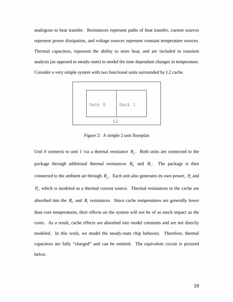
Consider a very simple system with two functional units surrounded by L2 cache.
Figure 2: A simple 2 unit floorplan
Unit 0 connects to unit 1 via a thermal resistance aR . Both units are connected to the
package through additional thermal resistances 0R and 1R . The package is then
connected to the ambient air through pR . Each unit also generates its own power, 0P and
1P , which is modeled as a thermal current source. Thermal resistances to the cache are
absorbed into the 0R and 1R resistances. Since cache temperatures are generally lower
than core temperatures, their effects on the system will not be of as much impact as the
cores. As a result, cache effects are absorbed into model constants and are not directly
modeled. In this work, we model the steady-state chip behavior. Therefore, thermal
capacitors are fully “charged” and can be omitted. The equivalent circuit is pictured
below.
Unit 0
Unit 1
L2

20
Figure 3: Steady-state equivalent thermal circuit for a dual unit system
Solving Kirchhoff’s Current Law for the above system yields the following results:
0 1 0 0 1 0 1 0 10 0 1
1 0 1 0
a p a p p a p p p
a a
R R R R R R R R R R R R R R R R R Rt p p
R R R R R R+ + + + + + +
= ++ + + +
(2)
0 1 0 1 1 1 0 0 11 0 1
1 0 1 0
a p p p a p a p p
a a
R R R R R R R R R R R R R R R R R Rt p p
R R R R R R+ + + + + + +
= ++ + + +
(3)
Or more generally:
0 0,0 0 0,1 1
1 1,0 0 1,1 1
t p pt p p
λ λ
λ λ
= +
= + (4,5)
where ,i jλ are constants composed of thermal resistances, and 0t and 1t are the
temperatures of each unit, above ambient. In addition, we propose (and will later
21
validate) that the power of a unit, can be approximated as a linear function of its
frequency. Therefore, if we assume a constant supply voltage, for a given unit x
x x x xp fα β= + (6).
Substituting (6) into (4) and (5),
( ) ( )( ) ( )
0 0,0 0 0 0 0,1 1 1 1
1 1,0 0 0 0 1,1 1 1 1
t f f
t f f
λ α β λ α β
λ α β λ α β
= + + +
= + + + (7,8)
distributing the constants λ , and renaming gives expressions of the form
0 0,0 0 0,1 1 0
1 1,0 0 1,1 1 1
t f ft f f
π π θ
π π θ
= + +
= + + (9,10)
Since all of the steady-state circuit components are linear, it can easily be shown that
solutions of higher numbers of units will always be linear combinations of f with an
additive factor θ . Thus, these results can be generalized in matrix form.
0,0 0,1 0,0 0 0
1,0 1,11 1 1
,0 ,
N
N N NN N N
t ft f
t f
π π π θπ π θ
π π θ
⎡ ⎤⎡ ⎤ ⎡ ⎤ ⎡ ⎤⎢ ⎥⎢ ⎥ ⎢ ⎥ ⎢ ⎥⎢ ⎥⎢ ⎥ ⎢ ⎥ ⎢ ⎥= × +⎢ ⎥⎢ ⎥ ⎢ ⎥ ⎢ ⎥⎢ ⎥⎢ ⎥ ⎢ ⎥ ⎢ ⎥
⎣ ⎦ ⎣ ⎦ ⎣ ⎦⎣ ⎦
L
L M
M M O MM M M
L L
(11)
or
T F= Π +Θ (12).
For our experiments, a single core has 17 different functional units. We thermally model
each unit independently while keeping a core’s units in the same clock frequency domain.
There are several possible models that could describe our system. We have
chosen this linear model for two main reasons. The first, is simplicity. Without an
overly complicated model for temperatures the parameters can be accurately fit with a

22
reasonable amount of machine learning. We will explain, in detail, our supervised
learning techniques and model validations in Chapter 4. The simplicity of our model will
also allow for calculations to be made on fine-grained time scales so as to be useful in
thermal management. The second purpose for using this simple linear model is that it fits
well with our optimization procedure: linear programming. Since all of the units’
temperatures are linear functions of frequency, the model elegantly fits into an
optimization framework that is well understood and can be solved quickly.
3.3 Optimization Using Linear Programming
Linear programming is a computational method for maximizing an objective
function subject to a set of linear constraints. In this work, we seek to maximize the total
physical performance across the processor, while using temperature as a constraint.
Thus, we use the linear system (12) to form constraint equations of the form below,
T F≥ Π +Θ (13).
This set of expressions (13), defines a multi-dimensional feasible space, within
which, the operating point of the system must lie. The linear program is very malleable.
It is possible to constrain the system to require positive frequencies ( 0F ≥ ). The system
may also be constrained to keep the core frequencies above (or below) a user defined
minimum (or maximum) threshold. Therefore, we choose to constrain a minimum value
on the clock frequencies of each core with another set of expressions:

23
0 min
1 min
minN
f ff f
f f
≥≥
≥M
(14)
and if minf is the same for every core,
minF f≥ (15).
Now with a fully defined feasible region in “frequency space,” we can define an
objective function that we wish to maximize. Additional constraints are omitted in this
work, but are easily integrated into the linear program. Power constraints, core frequency
equality constraints, maximum frequency constraints, etc, are all possible additions. Our
methods and models have been designed for malleability in order to include additional
optimization criteria.
The clock frequency of a core is the measure of a core’s physical performance.
Therefore, we wish to maximize a linear combination of the clock frequencies of each
core in order to maximize performance.
0 0 1 1... N NZ w f w f w f= + + (16)
or more generally,
TZ WF= (17)
where Z represents physical performance and is the quantity to be maximized, and W
represents the weight or importance of each process running on the system. If all of the
processes are of equal importance or urgency, the weight constant, W , will be a vector of
equal quantities. However, if a particular process running on a core is of high priority,
the weight constants can be adjusted.

24
There are several methods for solving linear programming problems. For this
work, we utilize the simplex method [13], which typically converges to a solution in
polynomial time. However, for worst case scenarios, the simplex method can converge
in exponential time. For our work, the algorithm was expected to converge in 2N or 3N
iterations, where N is the number of cores in the system. Thus, the simplex method was
more than efficient enough, but for complex systems of tens or hundreds of cores a
different method (such as an interior-point method) may prove more successful. We
leave this issue to further research.
Small changes in the weight constants, W , may not bring about a change in the
optimal point. Sensitivity analysis can be conducted at design/testing time. With the
sensitivity information in advance, it can be determined if a run-time change in the
weight constants W will bring about a new solution to the linear programming problem.
If the changes in W are sufficiently small, no time must be wasted solving the linear
program.
To better understand the effects of changes in W , consider again the two unit
system represented by the thermal constraints below
max 0,0 0 0,1 1 0
max 1,0 0 1,1 1 1
t f ft f f
π π θ
π π θ
≥ + +
≥ + + (18,19)
with the objective function
0 0 1 1Z w f w f= + (20)
and the minimum frequency constraints
0 min
1 min
f ff f≥≥
(21).
Plotting this system in “frequency space” gives fig. 4 below.

25
Figure 4: The optimal point in “frequency space” occurs at the intersection between the
maximized objective function and a vertex of the feasible region.
In this figure, blue orthogonal lines represent the minimum frequency constraints.
The additional blue lines represent a thermal constraint. Running the cores at frequencies
beyond this constraint would result in an on-chip temperature that is greater than the
specified value.
For this example, we keep the weight constants, W , at unity. The objective
function is plotted in red. We can shift the objective function (as indicated by the arrows)
until Z is maximized. This will always occur at a intersection between the objective
function and one of the feasible region’s vertices. The intersection (or the optimal point)
is marked by a box in the figure. Fig. 5 below shows the effect of small changes in W on
the objective function, and its resultant optimal point.
26
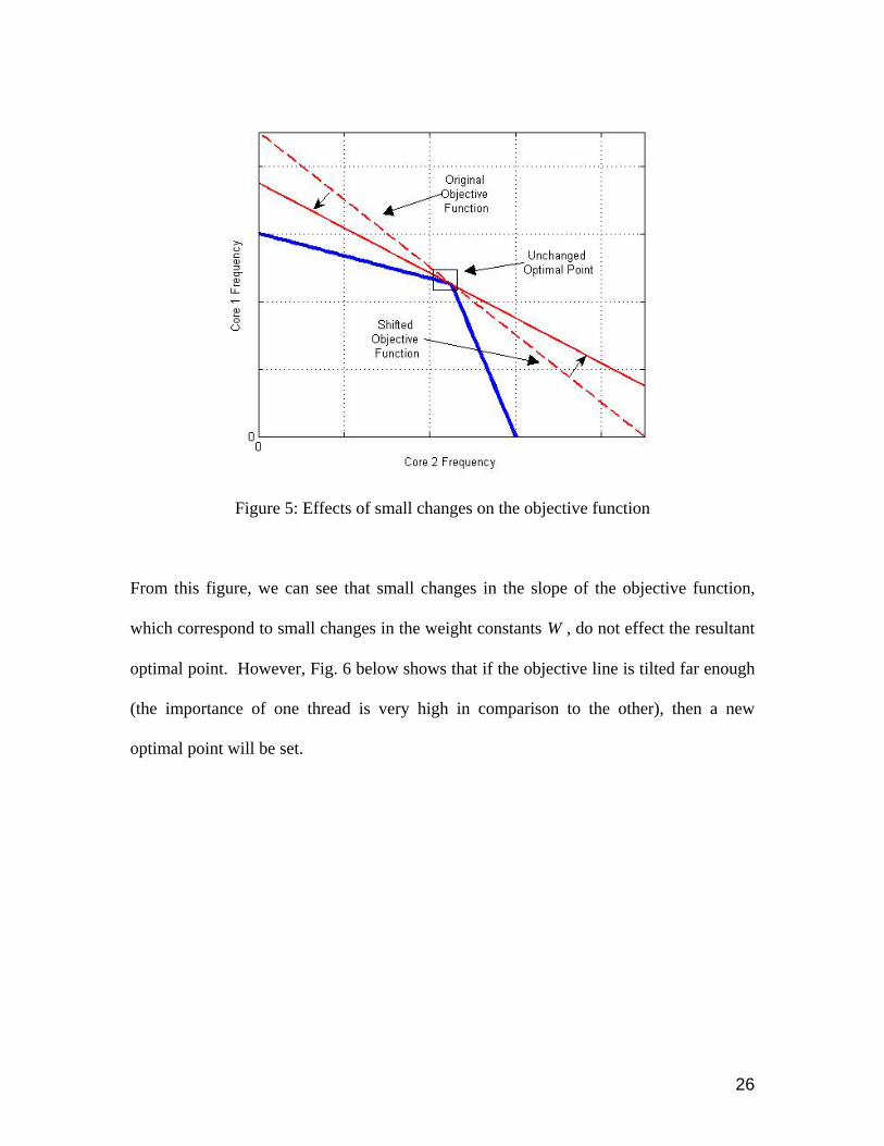
Figure 5: Effects of small changes on the objective function
From this figure, we can see that small changes in the slope of the objective function,
which correspond to small changes in the weight constants W , do not effect the resultant
optimal point. However, Fig. 6 below shows that if the objective line is tilted far enough
(the importance of one thread is very high in comparison to the other), then a new
optimal point will be set.

27
Figure 6: Tilting the objective function past the slope of the isothermal curve causes the optimal point to shift to a different vertex.
An analogous analysis can be completed in higher dimensional spaces (more cores). By
analyzing the sensitivity of our model, unnecessary optimization calculations can be
avoided, saving time and power at runtime.
3.4 Scaling Trends
In order to better predict the effects of our methods on many-core systems (16, 32,
and more cores) we must examine the physical changes in chip design that are likely to
occur in coming years. Admittedly, our scaling methodology is not overwhelmingly
rigorous. However, the purpose of this paper is not to model future scaling trends to a
high degree of accuracy. Rather, our work is in thermal management, and these “first-
order” scaling models have been designed to provide insight into future implementations

28
of our temperature-oriented methods. They have not been designed to be extremely
accurate models to be used outside of the scope of this work.
For our experiments, we examine 7 different technology settings using the Alpha
EV6 processor as our baseline core. Namely, 130nm (1 core), 90nm, (2 cores), 65nm (4
cores), 45nm (8 cores), 32nm (16 cores), 32nm with low cache power (16 cores), and
22nm with low cache power (32 cores). Each technology generation halves the area of a
given circuit, and doubles the number of transistors in the cache. Thus, transitioning
from one technology node to the next, doubles the number of cores, and doubles the
memory capacity of the cache.
Changes in supply voltages, threshold voltages, oxide thickness, and other
parameters cause changes in power values with technology. In order to model these
changes in power, we turn to the International Technology Roadmap for Semiconductors
[23]. This work provides a framework for the industry to follow as scaling proceeds into
the deep sub-micron regime. Assuming the ITRS trends are accurate, we use them to
formulate Table 1.
Transistor Type Bulk Silicon
Bulk Silicon
Bulk Silicon
FD SOI FD SOI FD SOI
Technology Node (nm)
130 90 65 45 32 22
Number of cores 1 2 4 8 16 32
Supply voltage (V)
1.3 1.2 1.1 1.0 .9 .8
Leakage current per micrometer of
width (uA)
.01 .05 .2 .22 .29 .37
Capacitance per micrometer width
(F)
1.15E-15 9.98E-16 6.99E-16 7.35E-16 6.18E-16 5.25E-16
Table 1: Scaling data
29
The ITRS report provides us with the expected supply voltage, expected leakage
current per micrometer of gate width, and expected gate capacitance at past, current, and
future technology nodes. Since our power model is native to the 65nm node, we must
scale these values, according to the ITRS, for the changes at other nodes. Table 1 is a
summary of the results from the ITRS scaling trends.
Consider a technology node k , with supply voltage, total gate capacitance, and
leakage current @kV , @kC , @kI , respectively. An individual core’s power can be
expressed as the sum of its dynamic and leakage powers,
@ ,@ ,@k d k l kP P P= + (21).
Since dynamic power is proportional to the square of supply voltage and proportional to
gate capacitance, and since leakage power is proportional to supply voltage and sub-
threshold current,
@ 1 ,@ 1 ,@ 1k d k l kP P P+ + += + (22)
@ 1 @ 1 @ 1 @ 1@ 1 ,@ ,@
@ @ @ @
12
k k k kk d k l k
k k k k
V V C IP P P
V V C I+ + + +
+
⎛ ⎞= +⎜ ⎟⎜ ⎟
⎝ ⎠ (23).
We introduce the 2 factor, because the total gate width scales by 2 from one
technology generation to the next. Note that (23) applies to the scaling of a single core.
To scale total chip-wide power, we must double the power provided by (23), assuming
that each technology generation doubles the number of transistors on chip. One
limitation of our model is that it does not incorporate the effects of global busses that
span chip-wide dimensions. We leave the scaling and power consumption of these
busses to future research.

30
In order to more accurately scale cache power, we use CACTI 5.0 [20]. CACTI is
an industry trusted cache access time and power calculator. We use CACTI’s high power
cache models at the technology nodes up to 32nm. Cache leakage power grows
exponentially with technology, and thus, an unreasonable amount of leakage power is
predicted at the 32nm and 22nm technology nodes (~150 W). Chip designers will have
to address this problem. Using low power transistors (with decreases in performance),
using “drowsy” cache methods, and other design techniques, designers will be able to
lower the amount of energy dissipated in the caches. It is difficult to quantify these
design improvements at future nodes. Therefore, at the 32nm node we run our
experiments with both high power and low power transistors, and for 22nm we use only
the low power transistors. This may not exactly model the power behavior of L2 caches
at future technologies. However, we use these low power models to gain insight into the
possibilities at these later nodes.
With the scaling trends in hand, it is now possible to characterize the thermal
model at various technology nodes, with various numbers of cores. The machine
learning techniques, and validity of the model will be assessed in the following chapter.

31
Chapter 4: Model Validation and Parameter Learning
4.1 Validating the Linear Frequency/Power Relationship
In order for our linear model to be a valid approximation of actual chip behavior,
we must first assure that our assumption in (6) is legitimate. In other words, we must
confirm that total power is a linear function of frequency. Dynamic power, by (1), is a
linear function of frequency. Leakage power, however, is only quasi-dependent on
frequency. Sub-threshold leakage is an exponential function of temperature. Increased
frequencies bring about higher dynamic power densities, which bring about increases in
temperature. Thus, we must assure, that a core’s “self-heating” does not cause enough
non-linearity to weaken the model.
To do this, we isolate a single core and run it through the iterative flow in fig. 1.
We vary frequency and plot the total (dynamic and leakage) core power at the various
technology nodes. Fig. 7 below shows the resultant total power vs. frequency for each
technology node.

32
Figure 7: Total power vs. clock frequency for a single core at several technology nodes.
Clearly, fig. 7 shows that despite exponential LDT behavior, a core’s total power
approximates a linear function of frequency. This confirms our claim in (6) is accurate.
Fig. 7 may be misleading, because it appears that the ratio of leakage power to dynamic
power is very small. It is true that, especially at later nodes, leakage power represents
much larger percentages of total power. However, the majority of the leakage power is
concentrated in the cache structures. Since fig. 7 is for cores only (the L2 cache is not
included), leakage plays a much smaller role.
33
4.2 Thermal Model Parameter Fitting and Validation
As stated above, the design space for many cores, at many frequencies, with
various test benchmarks is astronomical in size. Thus, it is impossible to fit our linear
model’s parameters to a real system’s behavior at all points. Instead, we must efficiently
sample the system and apply the model to the smaller data set. To do this, we run a
machine learning algorithm described by the pseudo-code below.
• Monte Carlo Simulation: o Input a random frequency/benchmark vector into the tool-
chain o Compute a multiple regression of all available data o Examine the mean error between the regression model and the
tool-chain outputs o If the mean error is unchanged from the previous iteration
Setup and solve the linear program with the model parameters (section 5.1)
Run the program solution through the tool-chain to assure proper steady-state temperature
o Else Repeat Monte Carlo Simulation
We begin by selecting a random frequency (on a reasonable range) and a random
benchmark for each core in the multi-core system. We input these vectors to the tool-
chain (fig. 1). This provides a resultant temperature vector. We use the temperature
vectors and the applied frequency vectors from all of the Monte Carlo iterations thus far,
and run a robust multiple linear regression. We use MATLAB to take the regression
using the least squares method. This method minimizes the sum of the squares of the
differences between the model and the observed data. Using the regression results, we
reapply the same frequency vectors to (12) and compare the model results with the

34
observed temperature from the tool-chain. We continue this procedure until the error
stabilizes.
A typical processor workload over time is more likely to be biased towards
integer or floating point benchmarks. A personal computer may be more likely to
compute integer threads than a high-performance server. In order to assess our model’s
validity on these more constrained workload sets, we also run Monte Carlo simulations
using random integer benchmarks only.
The absolute mean error for all of our Monte Carlo simulations ranged from .6%
to 2.8% depending on technology node. Generally speaking, our models are accurate to
within a 1-3 degrees C of the predicted temperature. A model accurate to this level is
more than capable of making thermal predictions accurate enough for thermal
management. As argued in [16], external factors like weather conditions and building
environmental controls can have effects on the order of a few degrees. Thus, a model
more accurate than ours, at added complexity, is likely to be superfluous.
4.3 Thermal Model Validation with an FPGA
We construct an experiment to assure that our thermal model actually does
represent the behavior of a multi-core system. Without the ability to monitor the
temperature of a commercial multi-core processor (such as an Intel Core 2 Duo), we
instead turn to a Field Programmable Gate Array (FPGA). We use a Cyclone II FPGA
on the Altera DE2 development board for our experiments.
35
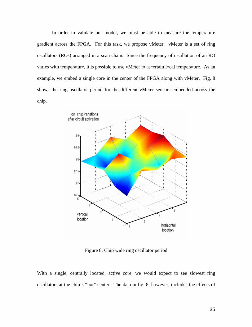
In order to validate our model, we must be able to measure the temperature
gradient across the FPGA. For this task, we propose vMeter. vMeter is a set of ring
oscillators (ROs) arranged in a scan chain. Since the frequency of oscillation of an RO
varies with temperature, it is possible to use vMeter to ascertain local temperature. As an
example, we embed a single core in the center of the FPGA along with vMeter. Fig. 8
shows the ring oscillator period for the different vMeter sensors embedded across the
chip.
Figure 8: Chip wide ring oscillator period
With a single, centrally located, active core, we would expect to see slowest ring
oscillators at the chip’s “hot” center. The data in fig. 8, however, includes the effects of

36
local on-chip process variations. Variations in oxide thickness and other process
parameters cause some ROs to be innately slower than others. In order to have this data
reflect temperature accurately, we also capture vMeter data with the core deactivated.
Subtracting away these inherent variations gives fig. 9.
Figure 9: Chip-wide temperature map
Fig. 9 clearly shows the thermal effects of the single active core. Thus, taking the
difference between vMeter’s readings during and before chip operation gives an on-chip
temperature gradient.

37
To test our multi-core model, we embed two NIOS II cores in two spatially
adjacent locations on the chip using the Altera development software’s “Logic Lock”
feature. We also include several vMeter sensors.
Figure 10: FPGA Floorplan
We use the DE2 development board’s 50MHz clock fed through a phase-locked
loop to produce 12.5, 25, and 75MHz clock signals. We multiplex these signals so that
any of the clock frequencies can be applied to either core. The Dhrystone benchmark is
run continuously and repetitively on both cores as the frequency is varied. Using the data
collected by vMeter, we use rigorous linear fitting techniques to fit the data to the form of
(12). We subsequently plot a contour map of the recorded data from vMeter.
Superimposed on this image, we include the isothermal lines from the model fit to the
FPGA data.

38
Figure 11: Observed contour map (color) and modeled isothermal lines (black)
Visually, the isothermal lines track the contour map correctly. Comparing the model’s
results with the observed data shows agreement to .5% mean absolute error. This
confirms that the model we have created is a reasonably accurate measure of multi-core
behavior in real silicon.
Having validated our well defined methods models and tools, we are now
prepared to run several experiments in thermal management, to assess the possible
performance gains brought about by our work.

39
Chapter 5: Experiments and Results
5.1 Frequency Planning
We solve the linear programming problem to maximize system performance. We
present two different solutions to the problem: a standard solution, and an optimal
solution. The standard solution has an added constraint equating the frequencies of every
core. This is the standard frequency plan in use in most chips today. If the design hyper-
space is perfectly symmetrical, than the optimal frequency plan, and the standard plan
will be the same. However, we have seen that core adjacency to various chip features, as
well as local variations in heat within the cores, have brought about asymmetry in the
hyper-space. Thus, we have seen much improved performance with the optimal
frequency plan, especially at later technology nodes.
We solve the linear programming problem defined by the constraints (13) and
(15), with the objective function (17). In this experiment, we set W from (17) to be a
vector of all ‘1’s. This indicates that each core is running a thread of equal importance.
We use the MATLAB optimization package’s linear program solver to ascertain the
optimal solution. Most optimizations took approximately .01 seconds on a 2.93GHz Intel
Dual Core Extreme workstation with 2GB RAM. This assures that the solutions could be
recomputed at run time in a dynamic thermal management setting. The results for the
various technology nodes are tabulated and plotted below.

40
Technology 130nm 90nm 65nm 45nm 32nm 32nm* 22nm Standard Integer Only Throughput
2.71 5.68 12.3 19.8 30.6 39.8 74.3
Optimal Integer Only Throughput
2.71 5.69 12.5 20.7 32.1 43.4 84.0
Standard Mixed-Benchmark Throughput
2.61 5.50 11.9 19.0 29.4 38.1 71.4
Optimal Mixed-Benchmark Throughput
2.61 5.53 12.1 19.9 30.8 41.6 80.8
Table 3: Throughput in billions of cycles per second for the standard and optimal
frequency plans. (* indicates low power caches)
Technology 130nm 90nm 65nm 45nm 32nm 32nm* 22nm Integer Only % Improvement
0 .2 1.6 4.3 4.6 8.3 11.5
Mixed-Benchmark % Improvement
0 .55 1.7 4.5 4.5 8.5 11.2
Table 4: Percent Improvement of the optimal plan over the standard frequency
plan (* indicates low power caches)
Figure 12: Throughput vs. technology node (mixed benchmark)
020406080
100
Throughput in Total GHz
65nm 32nmTechnology Node
Chip-Wide Throughput
Standard
Optimal

41
0
1
2
3
4
Frequency (GHz)
Optimal Frequency Plan
0
1
2
3
4
Frequency (GHz)
Standard Frequency Plan
Figure 13: Low power cache, 32nm, 16 core standard frequency plan and optimal
frequency plan (mixed benchmark) We see from table 3 and fig. 12 that there is a significant throughput improvement
for the optimal frequency plan over the standard plan. In addition, the improvement
seems to increase with technology. Moreover, the performance improvement with
coming generations does not just show increases in absolute performance, but in
percentage improvement as well (table 4). In other words, our methods will become
more effective at future technology nodes. With more cores on the chip, the thermal
advantages/disadvantages of adjacency become more evident and can be exploited more
easily by our methods.
We also see in fig. 13 the optimal frequency plan itself. In this figure, we can
clearly see that some cores have had their frequencies increased at the expense of other
cores. Fig. 13 shows one of the most important conclusions of our work. Cores
surrounded by other cores should be run at slower frequencies, while cores near the
comparatively cold cache or adjacent to the chip edge should be run at higher
frequencies. The colder caches and chip edges represent “thermal reservoirs” where heat

42
can more quickly and easily be transferred. Thus, outer cores can dissipate heat more
effectively and should be run faster. Interior cores, surrounded by comparatively hot
additional cores have less efficiency at dissipating their heat laterally, and can count only
on a heat transfer path through the package for heat removal. If an interior core is colder
than its surrounding cores, heat will also flow into the interior core from its neighboring
cores, only worsening its thermal disadvantage.
Thus, fig. 13 confirms that outer cores are much better candidates for frequency
increases, and interior cores should be run at slower frequencies. Also, corner cores have
two free sides, and thus can be run even faster. The integer units are located on one side
of the Alpha EV6 floorplan. As a result, cores that had their integer side near the cache
were able to be run faster in the integer only optimal plans.
To validate our solutions, we input both the optimal and standard frequency plans
into the tool-chain (fig.1). Across both workload sets and all technology settings, the
mean absolute error was 1.2 degrees Celsius. Thus, we have confirmed that applying the
optimal frequency plans to the chip actually does result in the desired steady-state
maximum temperature.
5.2 Process Priorities and Sensitivity Analysis
One of the most difficult aspects of the change to multi-core architectures will be
designing and compiling code from which a great deal of TLP can be extracted.
However, there will be unavoidable situations where the number of computable threads
and the number of cores may be different. In the case where the number of “ready”
threads is greater than the number of cores, the operating system will select which threads

43
are to be run on the available cores. In the case where the number of cores exceeds the
number of threads, the processing power of the vacant cores will be wasted.
In order to lower the performance penalty imposed by the stalled cores, we can
increase the speed of the cores with active threads. Their frequencies can be raised, since
cores can now more easily dissipate their heat horizontally to the cold stalled cores.
Assigning frequencies to the active cores can easily be accomplished by finding the
solution to our linear program. However, in this approach, the weight constants, W ,
from (17) will not all be unity. Instead, inactive cores should have no priority (weight
constant will be 0) and active cores will all have equal priority (weight constants will be
equal).
Figure 14: Throughput tradeoffs for different numbers of active cores
Fig. 14 shows the performance tradeoffs re-solving the linear program provides. The
figure shows that when the number of active cores is near 16, the possible performance

44
improvements are small. However, if 9 cores or less are active, re-solving the linear
program can bring significant improvements in throughput for the active cores. Since
there may be a small performance penalty associated with changes to the frequency
parameters for a core (i.e. resetting a phase-locked loop), chip-designers can decide
when re-solving the linear program and changing the core frequencies is worthwhile.
It is also prudent to examine the success of our methods in situations where all
cores are in use, but where the threads being run on said cores are of varying importance.
To illustrate the possible advantages of our system, we propose a simple case study.
Suppose a 16 core system is running 16 separate threads, 2 of which are of critical
importance to the user. The other 14 cores run tasks of low importance, that do not
directly interact with the user.
We begin with the optimal frequency solution from section 5.1 for 16 cores. We
assume the operating system would have already assigned the high priority threads to the
two fastest cores. We subsequently examine the time it would take to complete the two
high priority tasks as we vary their weight constants. The other low priority tasks will
have weight constants equal to unity.

45
Figure 15: Case study throughput. As the priority of the 2 high importance threads are increased, the time to complete those tasks decreases, but at the expense of decreases in
other cores’ performance. As fig. 15 shows, the speed of the high-priority cores can be increased, at the expense of
the speed of the low-priority cores. However, since the high-priority tasks were directly
visible to the user, quickly completing these tasks can greatly increase the observed
performance of a machine. The background tasks are not as time sensitive, and thus can
be sacrificed for the high-priority threads.
Chip, OS, and software designers can decide on how to assign weight constants to
each program, thread, or core. Using sensitivity analysis similar to this case study,
designers will be able to assign a weighting system to best optimize their system to boost
high-priority threads, while not completely sacrificing the needs of important background
threads.
5.3 Frequency and Voltage Planning
Because dynamic power scales with the square of voltage, and static power scales
directly with voltage, it is very difficult to construct an optimization methodology that
incorporates frequency and voltage scaling. We leave this addition to future work.
However, in order to show the potential performance improvements made possible by
true DVFS (as opposed to frequency scaling only as used in section 5.1), we have
developed a heuristic method. We use this method to show the possible performance
gains with the incorporation of voltage into our methods. This heuristic is non-optimal,
and takes extra computation to find a solution. However, it does provide some further
insight into even greater performance gains made possible by our methods.

46
To compute our voltage-incorporated solution, we first solve the linear program to
establish core frequencies without voltage scaling. We note the power consumed by each
core in the frequency plan. We adjust the frequencies/voltages such that the chip-wide
power distribution remains the same. We follow in suit with [13] and scale voltage by
V f∝ (24).
Thus, the supply voltage at a given frequency is given by
''
std
fV Vf
= (25),
where V designates the supply voltage for the frequency-optimal case calculated in
section 5.1, 'V and 'f designate the new parameters for the inclusion of voltage scaling,
and stdf is the reference frequency where voltage is at its nominal value.
A core’s total power is governed by
d sP P P= + (26).
Since dynamic power is a quadratic function of voltage and a linear function of
frequency, and since static power is a linear function of voltage, and since we wish to
keep the power profile constant,
2' ' '
d s d sV f VP P P PV f V
⎛ ⎞+ = +⎜ ⎟
⎝ ⎠ (27)
Combining (25) and (27) gives
( )2' '
d s d sstd std
f fP P P Pf f f
+ = +⋅
(28).
An analytical solution for 'f is extremely complex. Thus, we numerically iterate the
RHS of (28) until a value of 'f is found that makes the equality in (28) valid. We use

47
the solutions to redefine the frequencies from the optimal frequency plans for the
inclusion of voltage scaling. The results for each technology node are summarized in
tables 5 and 6 below.
Technology 130nm 90nm 65nm 45nm 32nm 32nm* 22nm Standard Throughput 2.61 5.50 11.9 19.0 29.4 38.1 71.4 Frequency Optimal Throughput
2.61 5.53 12.1 19.9 30.8 41.6 80.8
Voltage Heuristic Throughput
2.61 5.76 12.9 21.5 35.8 47.4 107.7
Table 5: Mixed benchmark throughput for standard, frequency optimal, and voltage incorporated heuristic plans.
Technology 130nm 90nm 65nm 45nm 32nm 32nm* 22nm Frequency Optimal Plan
0 .55 1.7 4.5 4.5 8.5 11.2
Voltage Heuristic 0 1.13 7.59 11.7 17.9 19.7 33.4
Table 6: Mixed benchmark percent improvement over the standard frequency plan for the frequency only and voltage heuristic plans.
Clearly, the effects of the supply voltage scaling only further the increases in
performance that we have reported in section 5.1. Since these results are not necessarily
optimal, tables 5 and 6 actually provide a lower bound for the possible performance gains
made possible by true DVFS as opposed to scaling frequency alone. Again, since DTM
techniques will already be in use at the core granularity, a performance gain of at least
33.4% can be obtained at the 22nm node with little or no additional hardware overhead.
Since the core-level chip-wide power profile is unchanged from the optimal
frequency plan, the same steady-state temperatures are measured as are measured in

48
section 5.1. Thus, the voltage-included results are also accurate to about 1.2 degrees
Celsius.
49
Chapter 6: Conclusions In coming generations, chip designers are likely to continue the trends towards
multi-core processors with multiple VFI’s. These processors will allow chips to continue
to increase their performance while maintaining a reasonable thermal budget. Since an
aggressive code piece, an external cooling malfunction, or some other effect may cause a
hotspot to form in a single core, and not chip wide, DTM methods have looked towards
core-level granularity for VFIs. We have presented a method for increasing chip-wide
performance that uses all of these existing design choices, with little extra cost.
We have proposed a very simple thermal model for multi-core systems. This
model allows us to calculate a core’s temperature to a reasonable degree of accuracy. We
have successfully fit the model to simulated data from industry accepted tools, as well as
to real silicon measurements on an FPGA. We have shown that the model fit both sets of
data to a reasonable degree of accuracy.
Our model fits elegantly into a linear programming optimization problem. We
have examined several different situations where the linear program provides an optimal
frequency plan that gives superior physical performance when compared to standard
frequency choices. Moreover, the optimization environment we have developed is
extremely malleable. If two cores are running threads that need to be computed at the
same time, those cores’ frequencies can be equated with an additional constraint in the
program. If there is a maximum power budget constraint, this can also be incorporated
into the program. If the chip design does not include individual VFIs for each core, but
rather for clusters of cores, it is a simple matter to equate each cluster’s frequency as a
50
constraint in the program. In addition, our model can be fit to any processor, any
floorplan, or any technology generation.
We have shown that performance gains can also be obtained in an all integer
workload. It is unlikely that a processor will always run a workload that is either entirely
integer or entirely floating point. Also, every chip fabricated from the same design may
not behave in exactly the same manner. These problems can be alleviated by leveraging
the existing temperature sensors on each core. Since multi-core DTM techniques will
require temperature input data from each core, this data can be stored along with
frequency data during chip operation. During down-time, or when single cores are
stalled waiting for a task, the processor can re-fit and re-compute the parameters of the
model with the recorded data. Since this data will be collected during run-time, it will
represent the most likely workload, and will most accurately reflect the real chip
behavior. This will assure that the model can most effectively leverage the possible
advantages/disadvantages of core location and workload type.
There are limits on the amount of TLP a workload can have. As a result,
situations may arise where all of the cores in a multi-core system are not in use. We have
shown that using our methods can help to increase the performance of a system with
stalled cores. Our method increases the active cores’ frequencies just enough to assure
the specified steady-state temperature constraint is not violated. Solving the linear
program does not just give a generic increase that can be applied to all cores. Rather, it
takes into account the spatial locality of stalled cores as well as the existing thermal
advantage/disadvantages of each core, and recomputes an optimal frequency plan. This
technique has a great deal of value at the current technology node, where multi-core
51
architectures are running workloads not necessarily designed for TLP. Even at future
nodes, there are fundamental limits to the TLP of a task, and thus, this technique for
boosting active core frequencies will be of incredible importance.
We have also analyzed the possible user-perceived performance increases
associated with priority values given to each of the threads being computed. By
increasing the weight of a certain thread, we have shown that that task can be sped up at
the expense of the other threads. In situations where some threads interact with the user
and some do not, the user-oriented threads can be completed more quickly. This will
help to increase continuity for the user. While this method may decrease the overall
throughput of the processor, the low-priority background tasks need not be completed
urgently. Furthermore, we have shown techniques for sensitivity analysis so that chip,
OS, and software designers can properly assign weight (priority) values to threads, in
order to maximize performance as desired.
The large performance gains that we have observed using our methodology make
a very strong case for keeping VFI granularity at the core level. Though energy
efficiency increases at this level of granularity may be small, the performance
improvements through our non-uniform frequency/voltage optimization methods are
significant. A frequency selection scheme like ours can best help to improve
performance by being given the opportunity to exploit as much thermal
advantage/disadvantage as possible. Restricting this ability with large VFI granularity is
a mistake.
Most importantly, all of these possible performance gains can be obtained with
very little hardware/software overhead. Since chips already have multiple cores, with
52
multiple VFIs, only adjustments to the thermal management unit’s control logic would be
necessary for implementation. Overall, these large performance gains, at little cost, are
likely to become essential as we move into the nanometer regime. Our method’s
malleability, its large performance improvements, and its scalability to the many-core
designs to come, make it an excellent steady-state thermal management system for future
multi-core processors.

53
References
[1 ] Ja Chun Ku et al., “Thermal management of on-chip caches through power density minimization,” Microarchitecture, 2005. MICRO-38. Proceedings. 38th Annual IEEE/ACM International Symposium on, 2005, p. 11 pp.
[2 ] C. Tsai and S.(. Kang, “Standard cell placement for even on-chip thermal distribution,”
Proceedings of the 1999 international symposium on Physical design, Monterey, California, United States: ACM, 1999, pp. 179-184; http://portal.acm.org/citation.cfm?id=300067.
[3 ] M. Mutyam et al., “Compiler-directed thermal management for VLIW functional units,”
SIGPLAN Not., vol. 41, 2006, pp. 163-172. [4 ] J. Donald and M. Martonosi, “Techniques for Multi-core Thermal Management:
Classification and New Exploration,” Computer Architecture, 2006. ISCA '06. 33rd International Symposium on, 2006, pp. 78-88.
[5 ] R. Mukherjee and S. Memik, “Physical Aware Frequency Selection for Dynamic
Thermal Management in Multi-Core Systems,” Computer-Aided Design, 2006. ICCAD '06. IEEE/ACM International Conference on, 2006, pp. 547-552.
[6 ]AMD Phenom Processor Datasheet, AMD, 2007; http://www.amd.com/us-
en/assets/content_type/white_papers_and_tech_docs/44109.pdf. [7 ] A. Kumar et al., “HybDTM: a coordinated hardware-software approach for dynamic
thermal management,” Proceedings of the 43rd annual conference on Design automation, San Francisco, CA, USA: ACM, 2006, pp. 548-553; http://portal.acm.org/citation.cfm?id=1146909.1147052&coll=Portal&dl=GUIDE&CFID=61233991&CFTOKEN=34737561.
[8 ] K. Skadron, “Hybrid Architectural Dynamic Thermal Management,” Proceedings of the
conference on Design, automation and test in Europe - Volume 1, IEEE Computer Society, 2004, p. 10010; http://portal.acm.org/citation.cfm?id=969045.
[9 ] K. Skadron et al., “Temperature-aware microarchitecture: Modeling and
implementation,” ACM Trans. Archit. Code Optim., vol. 1, 2004, pp. 94-125. [10 ] Tsorng-Dih Yuan, “Thermal management in PowerPC microprocessor multichip
modules applications,” Semiconductor Thermal Measurement and Management Symposium, 1997. SEMI-THERM XIII., Thirteenth Annual IEEE, 1997, pp. 247-256.
[11 ] R. Rao, S. Vrudhula, and C. Chakrabarti, “Throughput of multi-core processors under
thermal constraints,” Proceedings of the 2007 international symposium on Low power

54
electronics and design, Portland, OR, USA: ACM, 2007, pp. 201-206; http://portal.acm.org/citation.cfm?id=1283824.
[12 ] Wei Huang et al., “HotSpot: a compact thermal modeling methodology for early-stage
VLSI design,” Very Large Scale Integration (VLSI) Systems, IEEE Transactions on, vol. 14, 2006, pp. 501-513.
[13 ] S. Murali et al., “Temperature-aware processor frequency assignment for MPSoCs
using convex optimization,” Proceedings of the 5th IEEE/ACM international conference on Hardware/software codesign and system synthesis, Salzburg, Austria: ACM, 2007, pp. 111-116; http://portal.acm.org/citation.cfm?id=1289816.1289845.
[14 ] S. Herbert and D. Marculescu, “Analysis of dynamic voltage/frequency scaling in chip-
multiprocessors,” Proceedings of the 2007 international symposium on Low power electronics and design, Portland, OR, USA: ACM, 2007, pp. 38-43; http://portal.acm.org/citation.cfm?id=1283780.1283790.
[15 ] F.J. Mesa-Martinez et al., “Measuring performance, power, and temperature from real
processors,” Proceedings of the 2007 workshop on Experimental computer science, San Diego, California: ACM, 2007, p. 16; http://portal.acm.org/citation.cfm?id=1281700.1281716.
[16 ] H. Hanson et al., “Thermal response to DVFS: analysis with an Intel Pentium M,”
Proceedings of the 2007 international symposium on Low power electronics and design, Portland, OR, USA: ACM, 2007, pp. 219-224; http://portal.acm.org/citation.cfm?id=1283827.
[17 ] Weiping Liao, Lei He, and K. Lepak, “Temperature and supply Voltage aware
performance and power modeling at microarchitecture level,” Computer-Aided Design of Integrated Circuits and Systems, IEEE Transactions on, vol. 24, 2005, pp. 1042-1053.
[18 ] D. Brooks, V. Tiwari, and M. Martonosi, “Wattch: a framework for architectural-level
power analysis and optimizations,” Computer Architecture, 2000. Proceedings of the 27th International Symposium on, 2000, pp. 83-94.
[19 ] T. Austin, E. Larson, and D. Ernst, “SimpleScalar: an infrastructure for computer
system modeling,” Computer, vol. 35, 2002, pp. 59-67. [20 ] S. Wilton and N. Jouppi, “CACTI: an enhanced cache access and cycle time model,”
Solid-State Circuits, IEEE Journal of, vol. 31, 1996, pp. 677-688. [21 ] R. Kessler, E. McLellan, and D. Webb, “The Alpha 21264 microprocessor
architecture,” Computer Design: VLSI in Computers and Processors, 1998. ICCD '98. Proceedings. International Conference on, 1998, pp. 90-95.

55
[22 ] J. Henning, “SPEC CPU2000: measuring CPU performance in the New Millennium,” Computer, vol. 33, 2000, pp. 28-35.
[23 ]“International Technology Roadmap for Semiconductors”; http://public.itrs.net.