performance-based economical seismic design of multistory

UNLV Theses, Dissertations, Professional Papers, and Capstones

12-15-2018

Performance-Based Economical Seismic Design of Multistory Performance-Based Economical Seismic Design of Multistory

Reinforced Concrete Frame Buildings and Reliability Assessment Reinforced Concrete Frame Buildings and Reliability Assessment

Chunyu Zhang

Follow this and additional works at: https://digitalscholarship.unlv.edu/thesesdissertations

Part of the Civil Engineering Commons

Repository Citation Repository Citation Zhang, Chunyu, "Performance-Based Economical Seismic Design of Multistory Reinforced Concrete Frame Buildings and Reliability Assessment" (2018). UNLV Theses, Dissertations, Professional Papers, and Capstones. 3464. http://dx.doi.org/10.34917/14279204

This Dissertation is protected by copyright and/or related rights. It has been brought to you by Digital Scholarship@UNLV with permission from the rights-holder(s). You are free to use this Dissertation in any way that is permitted by the copyright and related rights legislation that applies to your use. For other uses you need to obtain permission from the rights-holder(s) directly, unless additional rights are indicated by a Creative Commons license in the record and/or on the work itself. This Dissertation has been accepted for inclusion in UNLV Theses, Dissertations, Professional Papers, and Capstones by an authorized administrator of Digital Scholarship@UNLV. For more information, please contact [email protected].

http://library.unlv.edu/

http://library.unlv.edu/

https://digitalscholarship.unlv.edu/thesesdissertations

https://digitalscholarship.unlv.edu/thesesdissertations?utm_source=digitalscholarship.unlv.edu%2Fthesesdissertations%2F3464&utm_medium=PDF&utm_campaign=PDFCoverPages

http://network.bepress.com/hgg/discipline/252?utm_source=digitalscholarship.unlv.edu%2Fthesesdissertations%2F3464&utm_medium=PDF&utm_campaign=PDFCoverPages

http://dx.doi.org/10.34917/14279204

mailto:[email protected]

PERFORMANCE-BASED ECONOMICAL SEISMIC DESIGN OF MULTISTORY

REINFORCED CONCRETE FRAME BUILDINGS

AND RELIABILITY ASSESSMENT

By

Chunyu Zhang

Bachelor of Science in Civil Engineering

Shenyang Jianzhu University

2009

Master of Science in Civil Engineering

Shenyang Jianzhu University

2012

A dissertation submitted in partial fulfillment

of the requirements for the

Doctor of Philosophy in Engineering – Civil and Environmental Engineering

Department of Civil and Environmental Engineering and Construction

Howard R. Hughes College of Engineering

The Graduate College

University of Nevada, Las Vegas

December 2018

ii

Dissertation Approval

The Graduate College

The University of Nevada, Las Vegas

November 16, 2018

This dissertation prepared by

Chunyu Zhang

entitled

Performance-Based Economical Seismic Design of Multistory Reinforced Concrete

Frame Buildings and Reliability Assessment

is approved in partial fulfillment of the requirements for the degree of

Doctor of Philosophy in Engineering – Civil and Environmental Engineering


Ying Tian, Ph.D. Kathryn Hausbeck Korgan, Ph.D. Examination Committee Chair Graduate College Interim Dean

Nader Ghafoori, Ph.D. Examination Committee Member

Mohamed Kaseko, Ph.D. Examination Committee Member

Samman Ladkany, Ph.D. Examination Committee Member

Mohamed Trabia, Ph.D. Graduate College Faculty Representative

iii

ABSTRACT

Performance-based Economical Seismic Design of Multistory Reinforced Concrete Frame

Buildings and Reliability Assessment

By

Chunyu Zhang

Dr. Ying Tian, Examination Committee Chair, Associate Professor



As the next generation of seismic design methodology, performance-based seismic design

(PBSD) method requires a structure satisfy multiple preselected performance levels under

different hazard levels. Optimal PBSD methods provide different strategies to design the

numerous variables, including strength, stiffness and ductility of each structural component. The

overall goal of this study is to develop a new optimal PBSD method for multi-story RC moment

frames. This method is capable of overcoming the deficiencies of existing optimal PBSD

methods and can be implemented by the U.S. design practice. The proposed method minimizes

construction cost and takes the limit of member plastic rotation and optionally inter-story drift as

iv

optimization constraints. Other seismic design requirements reflecting successful design practice

are also incorporated. Simplification is made by reducing design variables into two, one for the

overall system stiffness and the other for the overall system strength. The optimization contains

two stages, the determination of feasible region boundary in normalized strength and stiffness

domain and optimization in the material consumption domain. Capacity spectrum method, which

jointly considers nonlinear static analysis and inelastic design spectrum, is used to estimate the

global and local deformation demands at the peak dynamic response.

The proposed optimization approach is applied to the design of a six-story four-bay

reinforced concrete frame. The optimal design results indicate that 30% of needed flexural

strength and 26% of the cross-sectional area can be reduced from the initial strength-based

design of this prototype structure. Nonlinear time-history analyses are conducted on the

optimized structure using ten historical ground motions scaled to represent three levels of

seismic hazard. In general, the average peak dynamic response meets the target performance

requirements under the three levels of seismic hazard. Structural reliability analyses are applied

on the optimal structure, the original structure and other 26 structures with different overall

system stiffness and strength. The effects on nonperformance probability are determined based

on the nonperformance contours, which is generated based on the reliability analyses results of

all the 28 structures. To ensure the probabilities of nonperformance due to either plastic hinge or

inter-story drift rotation is lower than the limits of all three preselected performance levels, the

prototype structure should be design based on the relative overall system stiffness larger than

v

0.84 and the relative overall system strength larger than 0.4. To ensure that the probabilities of

nonperformance only due to plastic hinge is lower than the limits of all three preselected

performance levels, the prototype structure should be design based on two cases of relative

strength and relative stiffness: (1) the relative overall system stiffness is larger than 0.75 and the

relative overall system strength is larger than 0.4, and (2) the relative overall system stiffness is

larger than 0.65 and the relative overall system strength is larger than 0.45. To ensure that the

probabilities of nonperformance only due to inter-story drift rotation is lower than the limits of

all three preselected performance levels, a structure should be design based on the relative

overall system stiffness larger than 0.85 and the relative overall system strength larger than 0.6.

.

vi

ACKNOWLEDGEMENTS

I would like to express my sincere gratitude to Dr. Ying Tian, my dissertation supervisor.

His technical guidance was crucial for my Ph.D. research. Gratitude is extended to Dr. Nader

Ghafoori, Dr. Mohamed Kaseko, Dr. Samman Ladkany, and Dr. Mohamed Trabia for their

advice and serving on my dissertation committee. I would like to thank the support from the

Department of Civil and Environmental Engineering and Construction. I would like to thank my

mother, Li Yu, for her constant support and advice. I would like to offer special thanks to my late

father, Zhongliang Zhang, for his selfless devotion to our family and my growth.

Chunyu Zhang

December 2018

vii

TABLE OF CONTENTS

ABSTRACT....................................................................................................................................ⅲ

ACKNOWLEDGEMENTS............................................................................................................ⅵ

LIST OF TABLES.........................................................................................................................ⅺ

LIST OF FIGURES.......................................................................................................................ⅻ

CHAPTER 1. INTRODUCTION....................................................................................................1

1.1 Performance-based Seismic Design...................................................................................1

1.1.1 Conventional strength-based seismic design............................................................1

1.1.2 Concept of performance-based seismic design.........................................................4

1.2 Capacity Spectrum Method..............................................................................................12

1.2.1 Overview.................................................................................................................12

1.2.2 Demand spectra.......................................................................................................13

1.2.2.1 Elastic demand spectrum...............................................................................14

1.2.2.2 Highly damped demand spectra.....................................................................15

1.2.2.3 Inelastic demand spectra................................................................................16

1.2.3 Capacity spectrum...................................................................................................19

1.2.3.1 Pushover analysis...........................................................................................21

1.2.3.2 Transformation between MDOF and SDOF system......................................22

1.2.4 Estimation of nonlinear deformation demand.........................................................23

1.3 Displacement Coefficient Method...................................................................................26

1.4 Direct Displacement-based Seismic Design Methods.....................................................28

1.4.1 Structural wall.........................................................................................................29

1.4.2 SDOF systems.........................................................................................................31

1.4.3 MDOF systems.......................................................................................................32

1.4.4 Drawback of direct displacement-based seismic design method............................35

1.5 Optimal Performance-based Seismic Design Methods....................................................35

1.5.1 Optimal objectives..................................................................................................37

1.5.2 Optimization constraints.........................................................................................39

viii

1.5.2.1 Deterministic constraints...............................................................................40

1.5.2.2 Probabilistic constraints.................................................................................41

1.5.3 Optimal algorithms.................................................................................................43

1.5.3.1 Metaheuristics methods.................................................................................43

1.5.3.2 OC methods...................................................................................................48

1.6 Research Motivation........................................................................................................54

1.7 Research Objectives.........................................................................................................56

1.8 Research Methodology and Tasks....................................................................................57

CHAPTER 2 OPTIMAL PROFORMANCE-BASED SEISMIC DESIGN METHODOLOGY..59

2.1 Problem Statements.........................................................................................................59

2.1.1 Objective function...................................................................................................60

2.1.2 Constraints..............................................................................................................60

2.1.2.1 Performance constraints.................................................................................61

2.1.2.2 Seismic design constraints.............................................................................62

2.2 Optimal Methodology......................................................................................................65

2.2.1 Overview.................................................................................................................65

2.2.2 Simplifications........................................................................................................68

2.2.3 Determination of feasible region boundary.............................................................71

2.2.3.1 Overview........................................................................................................71

2.2.3.2 Load-deformation response due to modified flexural stiffness.....................73

2.2.3.3 Determination of minimum stiffness at given flexural strength....................76

2.3 Optimal Design Procedures.............................................................................................81

2.4 Extension of Proposed Optimal PBSD Method...............................................................84

2.5 Uniqueness of Proposed Optimal PBSD Method............................................................85

CHAPTER 3 IMPLEMENTATION OF PROPOSED OPTIMAL PBSD METHOD AND

EXAMINATION OF OPTIMAL DESIGN...................................................................................88

3.1 Implementation of Proposed Optimal PBSD Method.....................................................88

3.1.1 Initial design of original RC frame structure..........................................................88

ix

3.1.2 Finite element model...............................................................................................90

3.1.3 Optimization...........................................................................................................94

3.1.3.1 Feasible region boundary in λ‒α domain.......................................................94

3.1.3.2 Feasible region boundary in Ωc‒Ws domain and optimal design...................97

3.1.3.3 Construction cost reduction due to optimal design........................................99

3.2 Examination of the Optimal Design..............................................................................100

3.2.1 Hysteretic behavior model....................................................................................101

3.2.2 Earthquake record selection and scaling...............................................................102

3.2.2.1 Earthquake record selection.........................................................................102

3.2.2.2 Earthquake record scaling............................................................................104

3.2.3 Examination results and discussions.....................................................................108

3.2.3.1 Results of optimal design.............................................................................108

3.2.3.2 Result of original design..............................................................................112

3.3 Validity Verification of the Optimal Design..................................................................115

CHAPTER 4 RELIABILITY EVALUATION OF PROTOTYPE BUILDING..........................121

4.1 Overview of Reliability Evaluation...............................................................................121

4.2 Statistical Properties of Variables..................................................................................122

4.2.1 Statistical properties of external loads..................................................................124

4.2.1.1 Dead load and live load................................................................................125

4.2.1.2 Seismic load.................................................................................................126

4.2.2 Statistical properties of member resistance...........................................................128

4.2.2.1 Elemental flexural strength..........................................................................128

4.2.2.2 Elemental effective stiffness........................................................................129

4.2.3 Statistical properties of deformation limits...........................................................132

4.3 Sampling Methods.........................................................................................................134

4.3.1 Monte Carlo sampling method..............................................................................134

4.3.2 Latin Hypercube sampling method.......................................................................135

4.3.2.1 Procedure of Latin Hypercube sampling method........................................135

4.3.2.2 Elimination of correlation between variables..............................................138

4.4 Probability-based Nonperformance Probability.............................................................141

x

4.5 Fragility Curve Generation............................................................................................143

4.6 Results and Discussion..................................................................................................144

4.6.1 Normalized deformation.......................................................................................144

4.6.2 Nonperformance probability.................................................................................150

4.6.3 Fragility curve of nonperformance probability.....................................................151

4.6.4 Nonperformance probability contour....................................................................159

CHAPTER 5 SUMMARY AND CONCLUSIONS.....................................................................172

5.1 Summary........................................................................................................................172

5.2 Conclusions....................................................................................................................175

5.3 Suggestions....................................................................................................................177

REFERENCE...............................................................................................................................178

CURRICULUM VITAE..............................................................................................................190

xi

LIST OF TABLES

Table 1.1 Allowable inter-story drift ratio of RC frames in ATC-40 (1996), ASCE/SEI 41-06

(2007) and ASCE/SEI 41-13 (2014)........................................................................................9

Table 1.2 Allowable beam and column plastic hinge rotation capacity of RC moment frames in

ASCE/SEI 41-13 (2014) [θ] (unit: rad.)................................................................................10

Table 1.3 Target annual probabilities of nonperformance recommended by Paulay and Priestley

(1992).....................................................................................................................................43

Table 3.1 Flexural capacity of the elements in the original structure (unit: kip-in.)......................90

Table 3.2 Peak ground motion acceleration and velocity for three hazard levels..........................95

Table 3.3 Unit cost of material only and combined material and labor cost.................................98

Table 3.4 Comparison of cost for the initial and optimal designs...............................................100

Table 3.5 Details of selected ground motions.. ...........................................................................103

Table 3.6 Details of scaled ground motions.. ..............................................................................105

Table 3.7 Maximum standard deviation of inter-story drift ratios of optimal structure..............110

Table 3.8 Maximum standard deviation of inter-story drift ratio of original structure................114

Table 4.1 Summary of statistical properties of input variables....................................................124

Table 4.2 Composition of different types of nonperformance (unit: %)......................................145

Table 4.3 Normalized width of the 95% confidence band (w/a).................................................146

Table 4.4 Probabilities of nonperformance due to different types deformation of the optimal and

original structures.................................................................................................................150

Table 4.5 Probability of occurrence of the optimal and original structures under three hazard

levels (unit: %).....................................................................................................................155

xii

LIST OF FIGURES

Figure 1.1 Performance objectives determined by different target performance levels and

different hazard levels in ASCE/SEI 41-06 (2007)..................................................................6

Figure 1.2 Capacity spectrum method to predict structural non-linear deformation demand.......13

Figure 1.3 Elastic demand spectrum based on ASCE 7-10 (2010)................................................14

Figure 1.4 Highly damped demand spectra (Anil K. Chopra 2017)..............................................16

Figure 1.5 Elastic demand spectrum in different formats: (a) period vs. pseudo acceleration; (b)

spectral displacement vs. spectral acceleration......................................................................17

Figure 1.6 Elastic and inelastic demand spectra based on Vidic (1994)........................................19

Figure 1.7 Pushover analysis and capacity spectrum establishment: (a) the first mode shape and

the corresponding load pattern; (b) gravity and lateral loads; (c) top displacement vs. base

shear curve of MDOF system; and (d) capacity spectrum curve of SDOF system, and

demand spectra.......................................................................................................................20

Figure 1.8 Different equivalent methods to transform non-linear capacity spectrum curve to

equivalent bilinear capacity spectrum: (a) identical intersection and no post-yielding

stiffness; (b) different intersections and no post yield stiffness; and (c) identical intersection

and positive post-yielding stiffness........................................................................................25

Figure 1.9 Fanned radially-cracked region at the bottom of a structural wall and schematic strain

distribution at the base (Sasani 1998)....................................................................................29

Figure 1.10 Schematic diagram in Moehle (1992): (a) SDOF RC bridge pier; (b) idealized

flexural curvature; (c) elastic response spectrum...................................................................31

Figure 1.11 Target yield mechanism for moment frame (Goel et al. 2010)...................................33

Figure 1.12 The combined universal gravitation force and the universal gravitations caused by

the other masses (Rashedi 2009)............................................................................................45

Figure 1.13 Two steel frame examples in the study of Kaveh et al. (2010): (a) three-story

four-bay planar steel moment frame; (b) nine-story five-bay planar steel moment frame....47

Figure 1.14 Research methodology and procedure........................................................................58

Figure 2.1 Structural failure types: (a) beam-sway mechanism; and (b) soft story mechanism....62

Figure 2.2 Beam-sway mechanism and column flexural strength in the first floor.......................64

xiii

Figure 2.3 Framework of optimization: (a) optimization in material consumption domain; (b)

stiffness optimization for system with different strengths; (c) MDOF-SDOF transformation;

(d) nonlinear static analysis and determination of roof displacement demands; and (e) N2

method using inelastic spectra...............................................................................................66

Figure 2.4 Constructing based shear vs. roof displacement response based on nonlinear static

analysis result of the structure without stiffness modification (λ = 1)...................................76

Figure 2.5 Effects of modifying relative stiffness factor λ on capacity and demand curves.........78

Figure 2.6 Flow of the optimal PBSD method proposed in this study..........................................83

Figure 2.7 Illustration of the two times of optimal PBSD methods with (a) large interval; and (b)

small interval..........................................................................................................................84

Figure 2.8 Comparison of the searching method of different optimal algorithms: (a) OC method

proposed by Zou and Chan (2005); (b) and (c) optimal algorithm proposed in this study....86

Figure 3.1 Prototype RC frame building: (a) floor plan; and (b) elevation plan...........................89

Figure 3.2 Illustration of (a) location of the zero-length plastic hinge elements; (b) concentrated

plasticity model of one column; and (c) moment-rotation backbone curve of the plastic

hinge suggested byLignos and Krawinkler (2012)................................................................91

Figure 3.3 Transformation of loads: (a) two-way slab load distribution; (b) load combination; and

(c) equivalent concentrated loads...........................................................................................93

Figure 3.4 Feasible region of the six-story four-span RC moment frame in λ–α domain.............95

Figure 3.5 Feasible region boundary and optimal solutions in Ωc–Ws domain.............................97

Figure 3.6 Application of the capacity spectrum method to determine the seismic deformation

demands of occasional, rare, and very rare earthquakes........................................................99

Figure 3.7 Hysteretic behavior of modified Ibarra-Medina-Krawinkler model (Lignos and

Krawinkler 2012).................................................................................................................101

Figure 3.8 Time-history of unscaled horizontal ground acceleration for ten earthquakes...........104

Figure 3.9 Time-history of ten horizontal ground acceleration scaled according to very rare

earthquake level...................................................................................................................105

Figure 3.10 Time-history of ten horizontal ground acceleration scaled according to rare


Figure 3.11 Time-history of ten horizontal ground acceleration scaled according to occasional


xiv

Figure 3.12 Acceleration response spectra and scaled ground motions for different hazard levels:

(a) very rare earthquake; (b) rare earthquake; and (c) occasional earthquake.....................107

Figure 3.13 Peak inter-story drift ratio for optimal design subjected to ground motions scaled for

(a) occasional earthquakes; (b) rare earthquakes; and (c) very rare earthquakes................109

Figure 3.14 Ratio of average peak plastic hinge rotation demand to capacity (θmax/[θ]) for

optimal design subjected to ground motions scaled for (a) occasional earthquakes; (b) rare

earthquakes; and (c) very rare earthquakes..........................................................................111

Figure 3.15 Inter-story drift ratio for original design subjected to ground motions scaled for (a)

occasional earthquakes; (b) rare earthquakes; and (c) very rare earthquakes......................113


original structure subjected to ground motions scaled for (a) rare earthquakes and (b) very

rare earthquakes...................................................................................................................115

Figure 3.17 Feasible region and the design variables of nine structures in (a) λ–α domain and (b)

Ωc–Ws domain......................................................................................................................116

Figure 3.18 Peak inter-story drift ratio of the nine structures under rare earthquake derived from

dynamic analyses and the feasible region boundary determined from static analyses........118

Figure 3.19 Contours of the peak normalized inter-story drift ratio and the design variables of the

nine structures......................................................................................................................119

Figure 3.20 Construction cost of the nine structures for verifying the validity of the proposed

optimal PBSD method.........................................................................................................120

Figure 4.1 Probability density function (PDF) curve of: (a) normal distribution; and (b) Type Ⅰ

distribution...........................................................................................................................126

Figure 4.2 Probability density function curve of lognormal distribution....................................127

Figure 4.3 Measured ratio between effective stiffness and gross bending stiffness (Elwood

2007)....................................................................................................................................130

Figure 4.4 Distribution fitting of discrete stiffness ratio (a) frequency histogram of discrete

stiffness ratio and PDF of fitting lognormal distribution; (b) cumulate frequency histogram

of stiffness ratio and CDF of fitting lognormal distribution................................................131

Figure 4.5 Probability density function curve of Beta distribution.............................................133

Figure 4.6 Procedure of Latin Hypercube sampling method: (a) representative values selection

from CDF of one variable; (b) frequency histogram and PDF of selected representative

xv

values; (c) order rearranging of representative values of one variable; and (d) input data

matrix of all variables and samples......................................................................................136

Figure 4.7 Relationship between two variables: (a) correlation and (b) independent.................138

Figure 4.8 Illustration of the relationship between two input variables: (a) correlated relationship

(b) independent relationship................................................................................................141

Figure 4.9 Statistical result of the peak normalized plastic deformations (maximum value of γ/[γ]

and θ/[θ]) of the optimal and original design in various performance levels: (a) collapse

prevention; (b) life safety; and (c) immediate occupancy...................................................147

Figure 4.10 Statistical result of the peak normalized plastic deformations (peak θ/[θ]) of the

optimal and original design in various performance levels: (a) collapse prevention; (b) life

safety; and (c) immediate occupancy...................................................................................148

Figure 4.11 Statistical result of the peak normalized plastic deformations (peak γ/[γ]) of the

optimal and original design in various performance levels: (a) collapse prevention; (b) life

safety; and (c) immediate occupancy...................................................................................149

Figure 4.12 Fragility curves for the optimal design in different nonperformance types: (a) either

θ/[θ] > 1 or γ/[γ] > 1; (b) θ/[θ] > 1; and (c) γ/[γ] > 1...........................................................152

Figure 4.13 Fragility curves for the original design in different nonperformance types: (a) either

θ/[θ] > 1 or γ/[γ] > 1; (b) θ/[θ] > 1; and (c) γ/[γ] > 1...........................................................153

Figure 4.14 Defination of the four types of damage states..........................................................154

Figure 4.15 Probability histogram of four damage states of the (a) optimal and (b) original

structures..............................................................................................................................156

Figure 4.16 Fragility curves for both the optimal and original designs in different performance

levels: (a) collapse prevention; (b) life safety; and (c) immediate occupancy....................158

Figure 4.17 Probability contours of nonperformance due to inter-story drift for different

performance levels (a) collapse prevention' (b) life safety and (c) immediate occupancy

(unit: %)...............................................................................................................................161

Figure 4.18 Deformation demand of inelastic SDOF systems with identical stiffness but different

yield strength........................................................................................................................162

Figure 4.19 Probability contours of nonperformance due to plastic hinge rotation for different

performance levels (a) collapse prevention; (b) life safety and (c) immediate occupancy

(unit: %)...............................................................................................................................163

xvi

Figure 4.20 Probability contours of nonperformance due to either inter-story drift or plastic hinge

rotation for different performance levels (a) collapse prevention; (b) life safety; and (c)

immediate occupancy (unit: %)...........................................................................................166

Figure 4.21 Nonperformance contours due to (a) inter-story drift; (b) plastic hinge rotation; and

(c) either plastic hinge rotation or inter-story drift (unit: %)...............................................169

1

CHAPTER 1

INTRODUCTION

1.1 Performance-based Seismic Design

1.1.1 Conventional strength-based seismic design

Seismic design attempts to design a structure capable of resisting both gravity and

seismic loads. Strength, stiffness and inelastic deformation capacity influence the seismic

performance of a structure. The conventional strength-based seismic design method in the U.S.

embodied in ASCE 7-10 (2010) designs strength and stiffness based on elastic seismic analysis

results. According to this standard, seismic design can be performed based on results of static

analyses, such as equivalent lateral force method and modal response spectrum method, or

dynamic (time-history) analyses.

In ASCE 7-10 (2010), the widely used static methods start from externally applying

lateral seismic forces on a building, then design element stiffness, and finally design element

strength. The design seismic force for the structure, the total design base shear, is derived by

dividing the seismic force of an elastic single degree of freedom (SDOF) structure with identical

natural period by a strength reduction factor, R. The seismic force of the elastic SDOF structure

is determined by structural seismic weight and design spectra response acceleration and the

estimated structural vibration period, T. Design earthquake for design earthquake level shall be

modified based on given site type. T can be estimated by empirical equations or eigen-value

2

analyses. Normally, the lateral strength of a structure to resist seismic loads is designed to be

lower than that needed to maintain elastic response in severe earthquakes. Then the structure

would behave inelastically under moderate or severe earthquake to dissipate more earthquake

induced energy than an elastic structure. Therefore, the design seismic force is derived by

dividing design earthquake of the elastic structure by R. The value of R is determined based on

the observations of performance of certain structural type under severe earthquakes (Miranda and

Bertero, 1994).

The stiffness design, in ASCE 7-10 (2010), is performed by selecting section sizes of

structural elements based on structural design experience and architectural requirements. Then

the inelastic deformation of the structure is checked by comparing the estimated inter-story drift

ratio under design-level earthquake and the inter-story drift ratio limit given in ASCE 7-10

(2010). Because the structure performs nonlinearly under a design-level earthquake, the total

deformation demand, accounting for both elastic and inelastic deformations, can be estimated by

multiplying a deflection amplification factor, Cd, to the elastic inter-story drift. Element stiffness

shall be modified based on the checking result to make sure that the structure inter-story drift

ratio does not exceed the specified drift limit.

After section sizes are determined, the needed flexural strength of element can be

obtained based on the elastic analysis results of the structure under combined gravity and design

seismic force in multiple combinations. The controlling strength demand of each element under

multiple load combinations is selected to be the needed flexural strength.

3

Some inaccurate estimations about structural deformation demand and capacity exist in

the above procedure of the force-based seismic design method. First, T used to obtain the design

seismic force is derived from empirical equations or elastic analysis. However, the actual

vibration period keeps decreasing during seismic excitations causing nonlinear structural

performance, and may be far different from T. Second, R and Cd are identical for a specific type

of structure without considering its uniqueness. For example, in ASCE 7-10 (2010), R is

recommended as 8, and Cd as 5.5 for RC special moment-resisting frames regardless their floor

levels, spans and irregularity. This roughly determined value may lead inaccurate estimation of

structural ductility demand (Zameeruddin and Sangle, 2016).

Some observations of the structural damage made after the relatively recent earthquakes

in the U.S. and Japan, such as the Northridge earthquake (1994 M6.7) and the Kobe earthquake

(1995 M7.2), revealed the drawbacks of the conventional strength-based seismic design method.

In these earthquakes, although the structures generally performed well, they suffered unexpected

severe structural damage, and high economic loss due to dysfunction and prohibiting repair cost.

(Rainer and Karacabeyli, 2000; Ghobarah, 2001). The total financial loss of the Northridge and

Kobe earthquakes reached about $20 billion (Kircher et al., 1997) and $200 billion, respectively

(Bertero and Bertero, 2002).

The disadvantages of strength-based seismic design are (1) only life safety performance

level (i.e. life safety) is considered (Krawinkler, 1999; Ghobarah, 2001; Sung et al., 2009); (2)

non-linear behavior causing the damage of structure in different hazard levels cannot be

4

predicted directly; instead it is derived based on some inaccurate assumptions (Ghobarah, 2001;

Priestley et al., 2007; Sung et al., 2009); and (3) this method is lack of socio-economic

description or information, such as cost of repair, for decision making (Krawinkler, 1999).

1.1.2 Concept of performance-based seismic design

To avoid the deficiency in the conventional force-based method of seismic design,

performance-based seismic design (PBSD) method was proposed by the American scientists and

engineers in the early 1990s (Liu et al., 2004). PBSD is a progressive method, by which a

structure is designed to achieve a target performance objective under each specified hazard level

(Ghobarah, 2001). The performance objective is used to distinguish the acceptable or

unacceptable structures, and shall be different for diverse hazard levels, such as mediate and

severe earthquakes. Different from the conventional force-based method, which obtains

structural safety or serviceability with uncertain reliability, PBSD provides designers with a

method to select a performance objective for diverse hazard levels (Krawinkler, 1999).

As the next generation of seismic design methodology, PBSD has been a major focus of

earthquake engineering community. This method was included in: SEAOC Vision 2000 (1995),

ATC-40 (1996), FEMA 273 and 274 (1996), FEMA 356 (2000), ASCE/SEI 41-06 (2007) and

ASCE/SEI 41-13 (2014). These documents are evolutionary in the definition of performance

objectives, seismic evaluation and design methodologies; nevertheless, the basic concepts of

PBSD are identical (Ghobarah, 2001). In SEAOC Vision 2000 (1995), the framework of PBSD

was established to accommodate various performance objectives. Structural performance was

5

classified into five levels. Four different seismic design methods were included in this standard:

conventional force-based method, displacement-based method, energy-based method, and

prescriptive design method. In ATC-40 (1996), the performance levels of the structural and

non-structural elements were defined separately. In addition, capacity spectrum method, an

inelastic static method, was suggested to be incorporated in PBSD. Even though some flaws

existed within this method, it gave a good estimation of seismic deformation capacity and

demand (Priestley, 2000). In FEMA 273 and 274 (1996), PBSD related performance levels with

hazard levels to define performance objective. Structural performance was classified into four

performance levels: collapse prevention (CP), life safety (LS), immediate occupancy (IO), and

operational performance levels. Different seismic evaluation and design methods, from linear

static to nonlinear dynamic methods, were adopted for PBSD in FEMA 273 and 274 (1996).

Based on engineering practice and observations, the values of deformation limits, such as

allowable plastic hinge rotation, used to identify whether a structure meets a certain performance

level, were adjusted in FEMA 356 (2000), and followed by ASCE/SEI 41-06 (2007). Seismic

evaluation methods, such as the simplification of the factors used in displacement coefficient

method to predict the peak structure displacement demand, were updated in ASCE/SEI 41-06

(2007). The allowable plastic hinge rotations were slightly adjusted in ASCE/SEI 41-13 (2014).

Moreover, specific limit of inter-story drift deformation was eliminated from this standard.

Based on the standards mentioned above, it can be summarized that PBSD method

includes four important aspects: multiple performance objectives, criteria used to define the limit

6

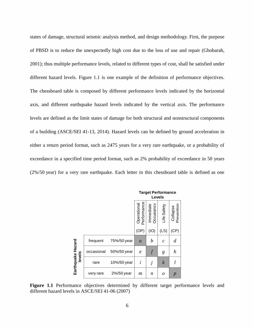
states of damage, structural seismic analysis method, and design methodology. First, the purpose

of PBSD is to reduce the unexpectedly high cost due to the loss of use and repair (Ghobarah,

2001); thus multiple performance levels, related to different types of cost, shall be satisfied under

different hazard levels. Figure 1.1 is one example of the definition of performance objectives.

The chessboard table is composed by different performance levels indicated by the horizontal

axis, and different earthquake hazard levels indicated by the vertical axis. The performance

levels are defined as the limit states of damage for both structural and nonstructural components

of a building (ASCE/SEI 41-13, 2014). Hazard levels can be defined by ground acceleration in

either a return period format, such as 2475 years for a very rare earthquake, or a probability of

exceedance in a specified time period format, such as 2% probability of exceedance in 50 years

(2%/50 year) for a very rare earthquake. Each letter in this chessboard table is defined as one

Figure 1.1 Performance objectives determined by different target performance levels and

different hazard levels in ASCE/SEI 41-06 (2007)

Target Performance

Levels

Op

era

tio

na

l

Pe

rfo

rma

nce

Imm

ed

iate

Occu

pa

ncy

Life

Sa

fety

Co

lla

pse

Pre

ve

ntio

n

(OP) (IO) (LS) (CP)

Ea

rth

qu

ak

e H

aza

rd

leve

ls

frequent 75%/50 year a b c d

occasional 50%/50 year e f g h

rare 10%/50 year i j k l

very rare 2%/50 year m n o p

7

performance objective, reflecting the target performance level under a certain hazard level. A

structure needs to satisfy all the selected performance objectives.

Based on ASCE/SEI 41-06 (2007), the performance objectives k and p in Figure 1.1, are

defined as the basic safety performance objectives, which are suitable for office, residential and

other general constructions. Nevertheless, some categories of buildings, such as schools,

hospitals and some government or communication buildings, are more important due to either

the unique social function or the needed ability to avoid large casualties. Thus, enhanced

performance objectives are applied on such buildings. The enhanced performance objective can

be a combination of a single basic safety performance objective and a lower performance

objective, such as the combination of k and o; alternatively, the enhanced performance objective

can be a combination of two lower performance objectives, such as j and o. If a building, such as

warehouse, is less important, the limiting performance objectives applied on its seismic designs

can be either a single basic safety performance objective, such as k or p alone, or any other single

higher performance, such as g.

The second aspect of PBSD is the acceptance criteria. To determinate whether a structure

can satisfy a certain performance level, criteria used to define the limited damage states shall be

explicitly quantified. The criteria can be a single criterion or a combination of allowable stress,

load, strain, displacement, acceleration and energy dissipation. Based on the study by Moehle

(1992), strain and deformation are more suitable for measuring damage than stress. Therefore,

PBSD can be deformation-based. However, in addition to deformation, structural damage is

8

affected by other parameters, such as the accumulation and distribution of structural damage, and

the failure mode of element and overall structure (Ghobarah, 2001). Thus comprehensive criteria,

considering both deformation and other influence factors, are used to describe the structural

damage states in some studies. For instance the Park and Ang damage index (Park and Ang, 1985)

consides both plastic deformation and dissipated energy under cyclic loading (Mechakhchekh

and Ghosn, 2007). Further studies are still likely needed for a more widely accepted criterion to

quantify structural damage states.

RC special moment-resisting frame is a conventional structural type. In the current

seismic evaluation standards in the U.S., the only explicit damage criteria of this structural type

are the deformation-based criteria, including allowable inter-story drift ratio and plastic hinge

rotation. The standards that include these two deformation indexes, are: ATC-40 (1996),

FEMA-273 (1996), FEMA-356 (2000), ASCE/SEI 41-06 (2007), and ASCE/SEI 41-13 (2014).

In these standards, the allowable interstory drift is given for three performance levels:

Immediate Occupancy (IO), Life Safety (LS), and Structure Stability (SS) in ATC-40 (1996) or

Collapse Prevention (CP) in all the other standards. Along the timeline of these standards, there

are two major advancements regarding the allowable values, as shown in Table 1.1. In ATC-40

(1996), the allowable inter-story drift ratio was given for only two performance levels as 2% for

LS performance level and 3.5% for SS performance level. Since FEMA-273 (1996), the

allowable interstory drift ratio was given for three performance levels. Note, in ASCE/SEI 41-13

(2014), there is no specific value for the allowable inter-story drift ratio, excepted for some

9

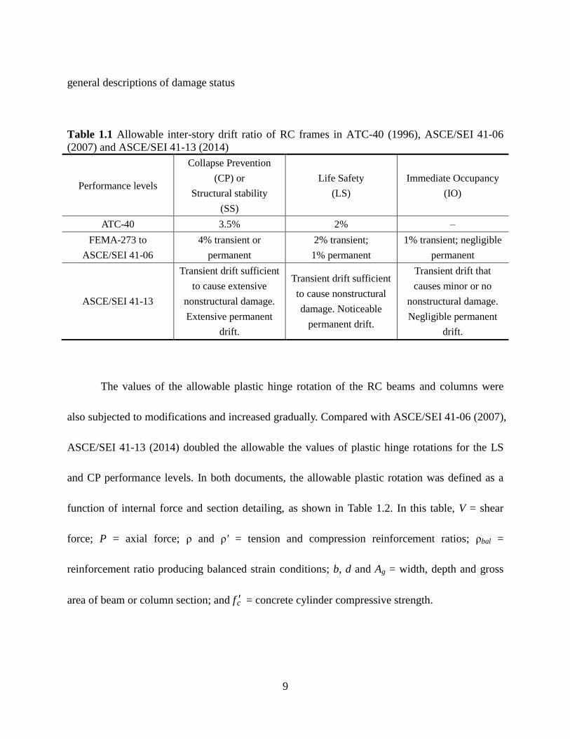
general descriptions of damage status

Table 1.1 Allowable inter-story drift ratio of RC frames in ATC-40 (1996), ASCE/SEI 41-06

(2007) and ASCE/SEI 41-13 (2014)

Performance levels

Collapse Prevention

(CP) or

Structural stability

(SS)

Life Safety

(LS)

Immediate Occupancy

(IO)

ATC-40 3.5% 2% ‒

FEMA-273 to

ASCE/SEI 41-06

4% transient or

permanent

2% transient;

1% permanent

1% transient; negligible

permanent

ASCE/SEI 41-13

Transient drift sufficient

to cause extensive

nonstructural damage.

Extensive permanent

drift.

Transient drift sufficient

to cause nonstructural

damage. Noticeable

permanent drift.

Transient drift that

causes minor or no

nonstructural damage.

Negligible permanent

drift.

11

The values of the allowable plastic hinge rotation of the RC beams and columns were

also subjected to modifications and increased gradually. Compared with ASCE/SEI 41-06 (2007),

ASCE/SEI 41-13 (2014) doubled the allowable the values of plastic hinge rotations for the LS

and CP performance levels. In both documents, the allowable plastic rotation was defined as a

function of internal force and section detailing, as shown in Table 1.2. In this table, V = shear

force; P = axial force; ρ and ρ' = tension and compression reinforcement ratios; ρbal =

reinforcement ratio producing balanced strain conditions; b, d and Ag = width, depth and gross

area of beam or column section; and f 'c = concrete cylinder compressive strength.1

10

Table 1.2 Allowable beam and column plastic hinge rotation capacity of RC moment frames in

ASCE/SEI 41-13 (2014) [θ] (unit: rad.)

Beam plastic hinge rotation capacity Column plastic hinge rotation capacity

ρ ρ

ρbal

c

V

bd f

Performance level

g c

P

A f c

V

bd f

Performance level

IO LS CP IO LS CP

≤ 0.0 ≤ 3 0.010 0.025 0.05

≤ 0.1 ≤ 3 0.005 0.045 0.060

≥ 6 0.005 0.020 0.04 ≥ 6 0.005 0.045 0.060

≥ 0.5 ≤ 3 0.005 0.020 0.03

≥ 0.6 ≤ 3 0.003 0.009 0.010

≥ 6 0.005 0.015 0.02 ≥ 6 0.003 0.007 0.008

The third aspect of PBSD method is structural analysis method. Diverse methods of

structural seismic analysis are available to estimate the nonlinear deformation demand on a

structure under a certain seismic hazard level. In PBSD, whether the structure satisfies the

selected performance level can be determined by comparing the estimated deformation demand,

in terms of plastic hinge rotation and inter-story drift ratio, with the corresponding deformation

criteria mentioned previously.

The structural analysis methods include dynamic time-history and static analyses. The

structural model used for these analyses can be either elastic or inelastic (nonlinear). To estimate

the structural nonlinear behavior under moderate or severe earthquakes, both nonlinear dynamic

and static analysis can be used. Normally, the dynamic time-history analysis provides a more

realistic structural response than the static methods, especially for moderate and severe

earthquakes and for tall buildings (Deierlein et al., 2010). However, this method is limited by the

high computational cost due to the need of using multiple earthquake records, and the sensitivity

to hysteretic model and ground motion selection (Elwood et al., 2007). The nonlinear static

11

method (pushover analysis) cannot effectively capture energy dissipation and lacks accuracy in

defining the strength and stiffness degradation of elements under cycle loading; however,

nonlinear static analysis is still widely adopted in practice due to its strong theoretical basis and

convenience. Both capacity spectrum method proposed by Fajfar (1999) and the displacement

coefficient method recommended in FEMA-273 (1996) to ASCE/SEI 41-13 (2014) can be used

to estimate the target displacement of the structure. These two methods are described with details

in Sections 1.2 and 1.3 respectively.

The fourth aspect of PBSD method is design methodology. Two types of PBSD

methodology exist: the iteration method by evaluating and modifying the force-based design

result, and the direct deformation-based method (Priestley, 2000; Zameeruddin and Sangle,

2016). The former method alternately applies performance-based structural analysis and

force-based seismic design. The structural analysis is used to check whether a structure meets the

selected performance objectives. If not, the force-based seismic design is applied to redesign the

structure. This process is repeated until all performance objectives are satisfied. This iteration

process significantly increases the computational cost of PBSD if multiple performance

objectives are to be satisfied (Priestley, 2000). Direct deformation-based method attempted to

incorporate deformation criteria in the preliminary design stage without an iteration process

(Priestley, 2000; Bertero and Bertero, 2002). This method is introduced in Section 1.4.

12

1.2 Capacity Spectrum Method

1.2.1 Overview

To estimate the nonlinear response of a structure under moderate and severe earthquakes,

several methods based on pushover analysis and demand spectra were proposed. In the pushover

analysis (Section 1.2.3.1), increasing lateral loads are monotonically applied along the height of

a multi-degree-of-freedom (MDOF) structure defined with inelastic properties. The MDOF

system is converted into an equivalent SDOF system (Section 1.2.3.2). In the equivalent SDOF

system, demand spectrum is used to estimate the deformation demand of a bilinear equivalent

single-degree-of-freedom (SDOF) system (Priestley 2000).

One of the nonlinear static methods was the N2 method proposed by Fajfar (1988 and

1996) using inelastic demand spectrum and pushover analysis results. A similar method called

capacity spectrum method was proposed by Freeman (1988) using highly damped demand

spectra and pushover analysis results. In this method, both capacity and demand spectrum was

expressed in spectral acceleration vs. spectra displacement format (Priestley, 2000). These two

methods were combined as a new version of capacity spectrum method based on the work of

Fajfar (1999). This method included both physical basis of inelastic demand spectra in the N2

method, and the convenient graphical procedure in the capacity spectrum method proposed by

Fajfar (2000).

Figure 1.2 shows the capacity spectrum method proposed by Fajfar (1999). The capacity

spectrum is obtained from pushover analysis results, and the demand spectrum is derived from

13

the elastic demand spectrum. Both of these spectra are expressed in spectral displacement (Sd) vs.

spectral acceleration (Sa) format. The demand spectrum intersects with the capacity spectrum.

The intersection between the capacity spectrum curve and the demand spectrum curve is used to

predict the seismic response of a structure under a single hazard level. An idealized bilinear

response is derived based on equivalent energy theory. Three aspects are included in the capacity

spectrum method: the demand spectrum establishment, the capacity spectrum establishment, and

the nonlinear deformation estimation based on the capacity spectrum and the demand spectrum.

These aspects are described in the following sections.

Figure 1.2 Capacity spectrum method to predict structural non-linear deformation demand

1.2.2 Demand spectra

Elastic demand spectrum can be generated based on the average value of the design

Sa

Sd

Intersection

Inelastic demand spectrum

Idealized bilinear capacity spectrum

Capacity spectrum

Elastic demand spectrum

Period of equivalent bilinear SDOF system

14

response spectra of historical earthquakes. Based on this elastic demand spectrum, two types of

demand spectra were proposed to reflect the effects of strength reduction of a nonlinear SDOF

system: highly damped demand spectra and inelastic demand spectra.

1.2.2.1 Elastic demand spectrum

Elastic demand spectrum can be generated by smoothing the response spectrum

constituted by the average spectral acceleration of SDOF systems with different natural period of

vibration. In addition, site type and system damping ratio also affect the elastic demand spectrum.

Figure 1.3 demonstrates a typical elastic demand spectrum of a system with 5% damping ratio

based on ASCE 7-10 (2010). Sae represents the elastic spectrum acceleration of the structures

with different natural periods of vibration.

Figure 1.3 Elastic demand spectrum based on ASCE 7-10 (2010)

In Figure 1.3, SMS and SM1 are respectively spectral response acceleration parameters at

0

0 4 0 6ae MS

TS S . .

T

SM1

SMS

T0 TS 1.0 TL

1M Lae

S TS

T

1Mae

SS

T

Medium

period

Long

period

Very long

periodShort

period

Sa (g)

T (sec.)

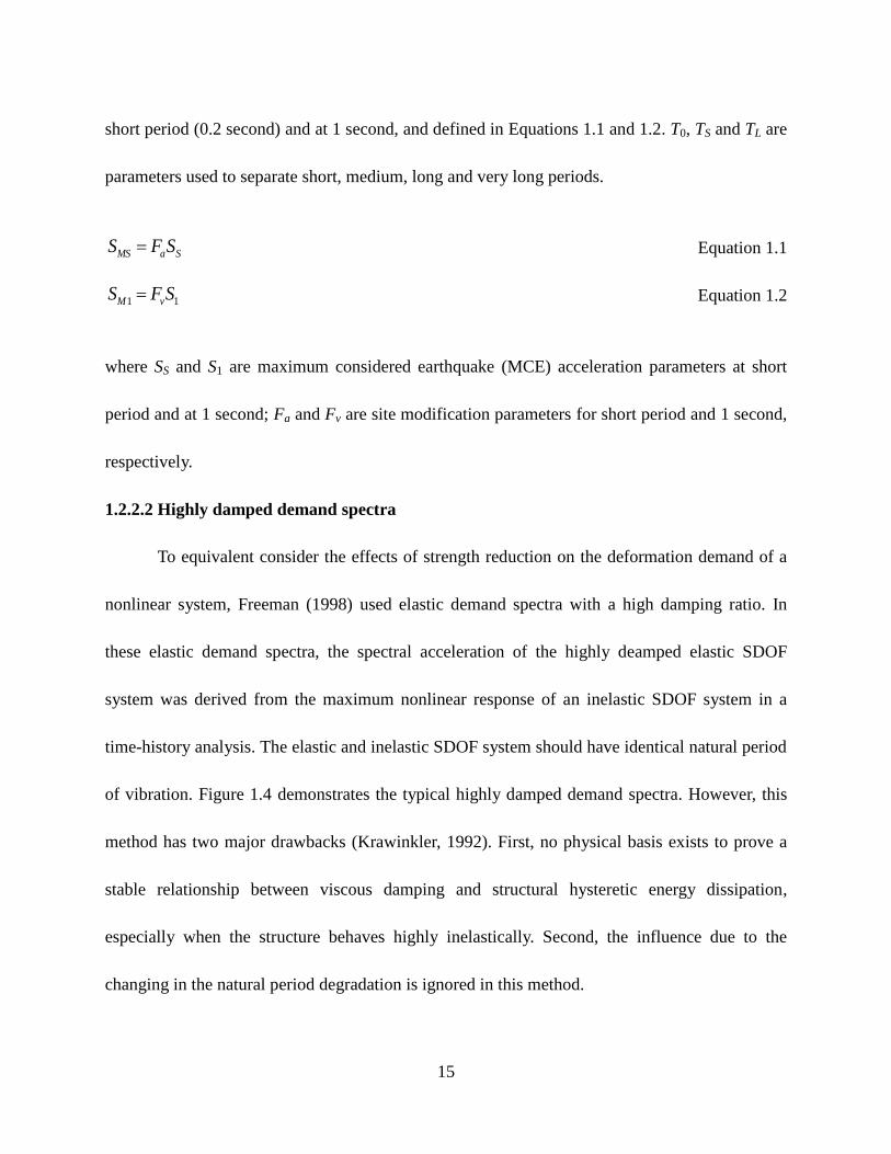
15

short period (0.2 second) and at 1 second, and defined in Equations 1.1 and 1.2. T0, TS and TL are

parameters used to separate short, medium, long and very long periods.

MS a SS F S

Equation 1.1

1 1M vS F S

Equation 1.2

where SS and S1 are maximum considered earthquake (MCE) acceleration parameters at short

period and at 1 second; Fa and Fv are site modification parameters for short period and 1 second,

respectively.

1.2.2.2 Highly damped demand spectra

To equivalent consider the effects of strength reduction on the deformation demand of a

nonlinear system, Freeman (1998) used elastic demand spectra with a high damping ratio. In

these elastic demand spectra, the spectral acceleration of the highly deamped elastic SDOF

system was derived from the maximum nonlinear response of an inelastic SDOF system in a

time-history analysis. The elastic and inelastic SDOF system should have identical natural period

of vibration. Figure 1.4 demonstrates the typical highly damped demand spectra. However, this

method has two major drawbacks (Krawinkler, 1992). First, no physical basis exists to prove a

stable relationship between viscous damping and structural hysteretic energy dissipation,

especially when the structure behaves highly inelastically. Second, the influence due to the

changing in the natural period degradation is ignored in this method.

16

Figure 1.4 Highly damped demand spectra (Chopra, 2017)

1.2.2.3 Inelastic demand spectra

To overcome the weakness of highly damped demand spectra, inelastic response

spectrum was proposed by some researchers, such as Veletsos et al. (1960, 1964), Newmark et al.

(1969), and Murakami and Penzien (1975). The parameters used to derive an inelastic demand

spectrum from an elastic demand spectrum are based on the statistical analysis of a SDOF

system with a bilinear force-displacement relationship (Fajfar, 1999). This inelastic demand

spectrum can more accurately estimate the peak nonlinear deformation than the highly damped

demand spectrum, especially for structures with short periods or high ductility demand (Fajfar,

1999, 2002).

Reinhorn (1997) suggested highly damped demand spectra should be in spectra

acceleration vs. spectra displacement format instead of the spectra acceleration vs. period format.

17

For an elastic SDOF system, the relationship among elastic spectral displacement, Sde, spectral

acceleration, Sae, and structural natural period of vibration, T, can be expressed by Equation 1.3.

Based on this equation, a smooth elastic demand spectrum in the spectral acceleration vs. period

format can be transformed into spectral acceleration vs. spectral displacement format, as shown

in Figure 1.5.

2

24de ae

TS S

Equation 1.3

(a)

(b)

Figure 1.5 Elastic demand spectrum in different formats: (a) period vs. pseudo acceleration; (b)

spectral displacement vs. spectral acceleration

The inelastic demand spectrum of a SDOF system with bilinear force-deformation

relationship can be derived from the elastic demand spectrum based on Equations 1.4 and 1.5.

μ

aea

SS

R Equation 1.4

Sa

(g

)

T (sec.)

Sd

(in

.)

Sa

(g)

Sd (in.)

T = 0.2 s.T = 0.5 s.

T = 1 s.

T = 2 s.

T = 5 s.

18

2 2

2 2

μ μ

μ μμ

4 4d de ae a

T TS S S S

R R

Equation 1.5

where Sa and Sd are the spectral acceleration and displacement of inelastic demand spectra,

respectively; T is structural natural period of vibration; Rμ is reduction factor considering

strength reduction of inelastic system to allow hysteretic energy dissipation; μ is ductility factor,

which is the ratio between the target displacement and the yield displacement of an equivalent

bilinear capacity spectrum.

Based on Equations 1.4 and 1.5, the accuracy of an inelastic demand spectrum depends

on the selection of appropriate values for Rμ and μ. Different versions of Rμ‒μ‒T relationship,

used to calculate Rμ based on μ, were proposed in the past decades (Newmark and Hall, 1982;

Nassar et al., 1992; Miranda and Bertero, 1994; and Vidic et al., 1994). Nevertheless, all these

Rμ‒μ‒T relationship provided similar results (Chopra and Goel, 1999). Equations 1.6 to 1.9

describe the latest Rμ‒μ‒T relationship provided by Vidic (1994). Figure 1.6 obtained by this

Rμ‒μ‒T relationship demonstrates the elastic demand spectrum and the inelastic demand spectra

with different μ.

1 0

0

μ 1 1Rc TR c T T

T Equation 1.6

1 0μ 1 1RcR c T T Equation 1.7

0 2 1μ TcT c T Equation 1.8

19

1 2v g

a g

c vT

c a Equation 1.9

where c1, c2, cR and cT are hysteretic behavior parameters, which can be defined as 1.35, 0.75,

0.95 and 0.2 for bilinear hysteresis model with 5% mass damping model; ag and vg are the peak

ground acceleration and velocity for a specified seismic hazard, respectively; cv and ca are

amplification factors for vg and ag, and can be defined as 1.8 and 2.5 for structures with 5%

damping ratio located in the U.S.

Figure 1.6 Elastic and inelastic demand spectra based on Vidic (1994)

1.2.3 Capacity spectrum

The capacity spectrum derived from a pushover analysis is used to predict structural

nonlinear deformation demand in the capacity spectrum method. Figure 1.7 demonstrates the two

Sa

(g

)

Sd (in.)

T=0.2 s. T=0.5 s.

T=1 s.

T=2 s.

T=5 s.

μ=1

μ=1.5

μ=2

μ=4

μ=6

μ=8

20

needed steps. First, pushover analysis is conducted on a MDOF system to obtain a top

displacement vs. base shear curve (Figure 1.7(a) and 1.7(b)). Second, the top displacement vs.

base shear curve for the MDOF system is transformed into a spectral displacement vs. spectral

acceleration curve in an equivalent SDOF system (Figure 1.7 (c) and 1.7(d)).

Figure 1.7 Pushover analysis and capacity spectrum establishment: (a) the first mode shape and

the corresponding load pattern; (b) gravity and lateral loads; (c) top displacement vs. base shear

curve of MDOF system; and (d) capacity spectrum curve of SDOF system, and demand spectra

Sa

(g

)

Sd

Vb

(k

ip)

Dt (in.)

Dt

Vb

Gravity loadsΦ Ψ = M Φ

M

(a) (b)

(c) (d)

MDOF

SDOF

P = pΨ

21

1.2.3.1 Pushover analysis

In the pushover analysis, lateral forces are monotonically applied on the structure. The

nonlinear behavior of the structure can be simulated by assigning distributed or concentrated

plasticity to the structural elements. During lateral loading, inelastic elements start to yield and

loss stiffness. Accordingly, the structure experiences stiffness degradation and behaviors

nonlinearly. The overall structural stiffness is affected by the nonlinearity presented in each

element. The most common measurement to reflect the overall nonlinear response of the

structure is the top (roof) displacement vs. base shear response, as shown in Figure 1.7(c).

The horizontal loads applied on the structure in a pushover analysis follow a certain load

pattern, as shown in Figure 1.7(b). Different load patterns have been suggested. The widely used

one is related to the first mode shape of the structure, as shown in Figure 1.7(a). This is rational

for the structures without abrupt changes of vertical strength or stiffness, since the first vibration

mode dominates such structures. Some other versions of load pattern were proposed to consider

higher mode effects (Park et al., 2007; Kreslin and Fajfar, 2012) or the variation of the load

pattern over time due to the inelastic response of the structure subjected to ground motions

(Gupta and Kunnath, 2000; Antoniou and Pinho, 2004).

Because the mass of each story is dominated by the slabs and the in-place stiffness of the

slabs is extremely high, the multi-story structure shown in Figure 1.7(b) can be simplified as an

lumped masses model with multiple lateral degrees of freedom (DOF) shown in Figure 1.7(a).

The lumped masses of the structure can be expressed by a diagonal matrix M. The mode shape

22

of this lumped masses model, Φ, can be obtained by an eigenvalue analysis. Then the lateral load

pattern used for the pushover analysis, P, can be determined by Equation 1.10. The lateral load

on the ith

floor, Pi, is expressed by Equation 1.11.

p p P Ψ MΦ Equation 1.10

i i iP pm Equation 1.11

where Ψ is lateral load pattern vector; p defines the magnitude of lateral load, and mi and Φi are

mass and mode shape on the ith

story.

1.2.3.2 Transformation between MDOF and SDOF system

The top displacement and base shear are used to reflect structural nonlinearity during

lateral loading, as shown in Figure 1.7(c). However, this top displacement vs. base shear curve

cannot be used together with the demand spectrum to predict structure deformation demand. This

is because this curve is for a MDOF system, while equivalent demand spectrum is for a SDOF

system. Therefore, a transformation of responses between the MDOF and SDOF systems is

needed.

Based on the equation of motion and assuming that the mode shape remains constant,

modal participation factor, Γ, is used to transform both the force and displacement of the MDOF

system to those of the SDOF system (Fajfar 1996 and 1999). Equation 1.12 defines Γ, and the

general mass of equivalent SDOF system, m*, can be obtained by Equation 1.13.

23

2 2=

T *i i

T

i i i i

m m

m m

Φ M1

Φ MΦ Equation 1.12

* T

i im m Φ M1 Equation 1.13

where Φ is mode shape; M is mass matrix of the lumped mass on each floor; mi and Φi are mass

and mode shape on the ith

story; 1 is a unit vector. It is noted that Φ is normalized by

proportionally modifying the mode shape vector until the roof displacement is equal to 1.

Top displacement, Dt, and based shear, Vb, of the MDOF system are transformed into

general displacement, D*, and general force F

*, of the equivalent SDOF system by Equations

1.14 and 1.15. The spectral acceleration corresponding to F* is defined by Equation 1.16.

* tDD

Equation 1.14

* bVF

Equation 1.15

*

a *

FS

m Equation 1.16

The capacity spectrum curve of SDOF system obtained based on the above derivation is

shown in Figure 1.7(d). However, since the inelastic demand spectrum is used for a SDOF

system with bilinear force-deformation relationship, the capacity spectrum shall also be

transformed into a bilinear format based on energy equivalence.

1.2.4 Estimation of nonlinear deformation demand

After deriving an inelastic demand spectrum and an equivalent capacity spectrum in the

SDOF system, an iterative procedure can be used to determine the intersection, which is used to

24

estimate the nonlinear deformation of the structure. Different methods of bilinear idealization

have been proposed. All were based on energy equivalency, that is, the area enveloped by

capacity spectrum should be identical to that enveloped by the bilinear equivalent capacity curve.

Figure 1.8 shows three equivalent transformation methods, where Kini. and Keff. are the initial and

effective structural stiffness; α is a strain hardening ratio for the post yield segment; Say and Sdy

are yield acceleration and displacement; Sae and Sde are elastic spectral acceleration and

displacement; Sai and Sdi are strength and displacement at the intersection between the bilinear

capacity spectrum and the non-linear demand spectrum.

The first method requires post yield stiffness be equal to zero, that is, no strain hardening

is assumed. Additionally, the three curves (non-linear capacity curve, equivalent bilinear capacity

curve and non-linear demand spectrum) intersect at the identical point, as shown in Figure 1.8(a).

The second method requires the post-yielding stiffness be equal to zero, and the corresponding

strength of the first intersection between the equivalent bilinear capacity curve and non-linear

capacity curve be equal to 60% of the yield strength, as shown in Figure 1.8(b). The third method

has a strain hardening, and the three curves intersect at the same point, as shown in Figure 1.8(c).

After the intersection between the capacity spectrum and the demand spectrum is

determined, the demands of deformation and force, and some other information, such as the

reduction factor, can be derived based on this intersection. The peak top displacement of the

MDOF structure, Dt, can be obtained based on Equation 1.14 and the spectrum displacement, D*.

All the external forces and element deformations are recorded in the pushover analysis for an

25

Figure 1.8 Different equivalent methods to transform non-linear capacity spectrum curve to

equivalent bilinear capacity spectrum: (a) identical intersection and no post-yielding stiffness; (b)

different intersections and no post yield stiffness; and (c) identical intersection and positive

post-yielding stiffness

Sae

Sa (g)

Say

Sdy Sde

Kini.

1

1Keff.

Sd (in.)Sdi

Elastic demand

spectrum

Non-linear

demand spectrum

T *

Sae

Sa (g)

Say

Sdy SdeSd (in.)Sdi

0.6Say

Elastic demand

spectrum

Non-linear

demand spectrum

Kini.

1

1Keff.

T *

Sae

Sa (g)

Say

Sdy SdeSd (in.)Sdi

Sai

Elastic demand

spectrum

Non-linear

demand spectrum

Kini.

1

1Keff.

1 αKeff.

T *

(a)

(b)

(c)

26

increasing Dt. Once Dt is determined, the corresponding records can be obtained. Furthermore,

Equations 1.17 to 1.20 can be used to determine Rμ, μ and the elastic period of the equivalent

bilinear SDOF system T*.

Equation 1.17

Equation 1.18

Equation 1.19

Equation 1.20

where F*

y and D*

y are the yield strength and displacement of the equivalent bilinear SDOF

system for capacity spectrum, respectively. In this study, the equivalent method shown in Figure

1.8(a) is adopted, because it can clearly define the factors of R-μ-T relationship (reduction factor,

Rμ, ductility factor, μ, and equivalent structural period of bilinear SDOF system, T*) for both

demand and capacity spectra.

1.3 Displacement Coefficient Method

In addition to the capacity spectrum method, displacement coefficient method can be

alternatively used to predict the maximum inelastic deformation of a structure. This method was

suggested in FEMA-273 (1996) to ASCE/SEI 41-13 (2014) to estimate the target roof

displacement, δt, based on the roof displacement vs. base shear curve derived from a pushover

μae

ay

SR

S

μ de de

*

y dy

S S

D S

2

* *

y*

*

y

m DT

F

* *

y ayF S m

27

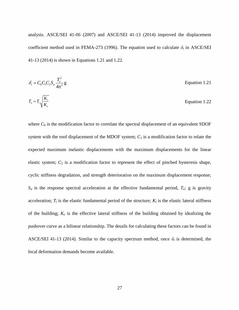
analysis. ASCE/SEI 41-06 (2007) and ASCE/SEI 41-13 (2014) improved the displacement

coefficient method used in FEMA-273 (1996). The equation used to calculate δt in ASCE/SEI

41-13 (2014) is shown in Equations 1.21 and 1.22.

2

0 1 2 2g

4

et a

TC C C S

Equation 1.21

ie i

e

KT T

K Equation 1.22

where C0 is the modification factor to correlate the spectral displacement of an equivalent SDOF

system with the roof displacement of the MDOF system; C1 is a modification factor to relate the

expected maximum inelastic displacements with the maximum displacements for the linear

elastic system; C2 is a modification factor to represent the effect of pinched hysteresis shape,

cyclic stiffness degradation, and strength deterioration on the maximum displacement response;

Sa is the response spectral acceleration at the effective fundamental period, Te; g is gravity

acceleration; Ti is the elastic fundamental period of the structure; Ki is the elastic lateral stiffness

of the building; Ke is the effective lateral stiffness of the building obtained by idealizing the

pushover curve as a bilinear relationship. The details for calculating these factors can be found in

ASCE/SEI 41-13 (2014). Similar to the capacity spectrum method, once δt is determined, the

local deformation demands become available.

28

1.4 Direct Displacement-based Seismic Design Methods

Direct displacement-based design (DDBD) method starts from the target (allowable)

displacement estimation of a structure under a selected hazard level or a selected performance

level. The structure is designed to be capable of resisting the target displacement (Priestley et al.,

2007; Welch et al., 2014). The seismic response of a structure is controlled by four quantities:

strength, stiffness and ductility. Normally, in the direct displacement-based design method, one

or two of these quantities is predetermined first to predict the target displacement demand. Then

the other quantities are determined by assuming displacement capacity is equal or slightly larger

than displacement demand (Fajfar 1999). The nonlinear displacement demand can be obtained

based on displacement response spectrum and structural effective stiffness or period (Moehle,

1992; Sasani, 1998). Alternatively, the nonlinear displacement demand can be estimated based

on the assumed displacement shape related to the inelastic first-mode at the design level of

seismic excitation and the selected ductility (Priestley et al., 1996; Priestley et al., 2007). In a

direct displacement-based design, the displacement capacity of a structure can be expressed and

limited by either allowable material strain or inter-story drift ratio. One drawback of direct

displacement-based design method is that this method designs structure based on only one

performance objective; thus, an iteration method may have to be used to modify structural

capacity so that the other performance objectives can be satisfied. The following sections briefly

describe the existing direct displacement-based design methods used for structural walls, SDOF

bridge piers and MDOF RC moment frames.

29

1.4.1 Structural wall

Sasani (1998) proposed a direct displacement-based design method for RC structural

walls resisting strong ground motions, as shown in Figure 1.9. First, this method designs a RC

wall under frequent earthquakes based on the traditional force-based method. At this hazard level,

the structure is expected to remain elastic, and its design is controlled by the deformation

requirements of the non-structural elements. Second, a direct displacement-based design is used

to estimate the structural deformation demand at the life safety performance level. Setting the

structural deformation capacity to be identical to the deformation demand, the concrete

compressive strain related to deformation capacity is checked. If this strain is larger than the

allowable value, then the design should be modified until the concrete strain is no more than its

limit. Finally, the base shear was checked to avoid an unexpected failure mode. The details of

this method are described below.

Figure 1.9 Fanned radially-cracked region at the bottom of a structural wall and schematic strain

distribution at the base (Sasani 1998)

30

The nonlinear deformation demand of a RC structural wall was assumed as 1.5 times of

the elastic deformation demand, which could be determined by the displacement response

spectra and an estimated structural fundamental period, T. T of the structure with N pieces RC

wall was obtained by Equation 1.23.

2

1

1 8N

eq

i

mT . H

EI

Equation 1.23

where H = wall total height; m = the average linear mass along wall height; and EIeq =

estimated equivalent flexural stiffness.

The equal displacement rule assumes that the peak inelastic deformation of a structure

under a strong ground motion is equal to the peak elastic deformation if the structure remains

elastic. However, based on the study by Wallace and Moehle (1992), the equal displacement rule

is not suitable for RC structural walls, and the ratio between the inelastic deformation and the

elastic deformation shall be 1.5. This ratio was adopted in the direct displacement-based design

method for walls. The deformation capacity at the top of the RC wall, Δt

c, was expressed as:

2

/ 23.6

yt

c u y p p

HL H L

Equation 1.24

where Φu and Φy are the yield and ultimate curvatures of the section; and H and Lp are wall total

height and plastic hinge length. Φy can be calculated as Φy = Mu/EIeq, where Mu is section

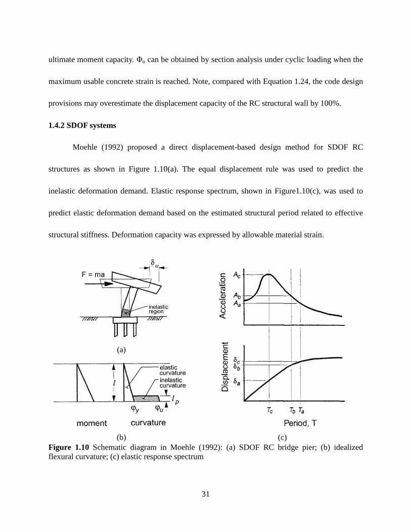
31

ultimate moment capacity. Φu can be obtained by section analysis under cyclic loading when the

maximum usable concrete strain is reached. Note, compared with Equation 1.24, the code design

provisions may overestimate the displacement capacity of the RC structural wall by 100%.

1.4.2 SDOF systems

Moehle (1992) proposed a direct displacement-based design method for SDOF RC

structures as shown in Figure 1.10(a). The equal displacement rule was used to predict the

inelastic deformation demand. Elastic response spectrum, shown in Figure1.10(c), was used to

predict elastic deformation demand based on the estimated structural period related to effective

structural stiffness. Deformation capacity was expressed by allowable material strain.

(a)

(c)

(b)

Figure 1.10 Schematic diagram in Moehle (1992): (a) SDOF RC bridge pier; (b) idealized

flexural curvature; (c) elastic response spectrum

32

The flexural deformation capacity of a SDOF bridge pier shown in Figure 1.10 could be

determined using Equation 1.25 proposed by Priestley and Park (1987).

2φ

δ φ φ3 2

y p

u u y p

l ll l

Equation 1.25

where δu is ultimate displacement capacity; l and lp are column height and plastic hinge length;

φu and φy are ultimate and yield curvatures of plastic hinge, respectively. φy can be neglected if

an idealized bilinear force-displacement model is used. φu can be determined by allowable

material strain, controlled by either the maximum usable concrete compression strain or the

longitudinal reinforcement tensile strain.

1.4.3 MDOF systems

Goel et al. (2008 and 2010) suggested a direct displacement-based design method for

MDOF frame structures based on the beam hinging mechanism shown in Figure 1.11 and a

pre-selected target drift. An equivalent energy method was used to determine the required base

shear force for different hazard levels. Therefore, multiple performance targets could be

considered simultaneously by selecting the largest base shear for design. Then the design base

shear was distributed vertically on each floor. A plastic design method was adopted to design

beam components based on the virtual work principle. The design base shear of one performance

objective, Vy, is calculated based on Equations 1.26 to 1.28.

33

Figure 1.11 Target yield mechanism for moment frame (Goel et al. 2010)

2 2α α 4γ

2

a

y

SV W

Equation 1.26

2

21

θ 8πα λ

g

Np

i i

i

hT

Equation 1.27

2

μ

2μ 1γ

R

Equation 1.28

where α reflects the target deformation demand; γ is an energy modification factor; Sa is the

design acceleration of one hazard level; θp represents the inter-story drift limit of one

performance level; W is total weight; T is structural vibration period; λi and hi are story height of

the ith

story and the corresponding distributed lateral load; Rμ is a strength reduction factor; and μ

is ductility ratio. The base shear of a performance target can be calculated according to the

selected hazard level and the desired performance level reflected by Sa and θp, respectively.

34

Then the design base shear, controlled by one of the multiple performance objectives,

was distributed vertically to each story considering the influence of higher mode and structural

nonlinearity, as shown in Equations 1.29 and 1.30.

0.20.75

1

1

β β

T

n ni i i yn

j j

j

w hF V

w h

Equation 1.29

0.20.75

β

Tn

j j

j i

i

n n

w h

w h

Equation 1.30

where Fi is the distributed lateral force at the ith

story; βi is a base shear distribution factor for the

ith

story; and wj and hj are the weight and height of the jth

story.

Finally, the plastic design method is used to design the yield strength of the beams

according to the distributed lateral loads. Virtual work principle is used by assuming the external

work caused by the distributed lateral load is equal to the internal virtual work caused by the

plastic hinge rotation at beam ends, as shown in Equation 1.31.

1 1

θ 2 θ 2 βn n

i i pc i pb

i i i

LF h M M

L

Equation 1.31

where θ represents the target plastic hinge rotation angle of the structure shown in Figure 1.11;

Mpb and Mpc are the design yield moments of the beams and the columns; L and L'

i are the total

35

and clear lengths of a beam. Mpc can be determined based on beam-hinge mechanism to avoid a

weak story. The design procedure based on Figure 1.11 implied that plastic hinges appeared at

each beam end and rotate with same angle under a strong earthquake, which may not be true.

1.4.4 Drawback of direct displacement-based seismic design method

Even though direct displacement-based design is considered a PBSD method, some

disadvantages exist. First, economy is a basic demand of PBSD method (Krawinkler, 1999), but

not directly involved in the existing direct displacement-based design methods. Moreover, more

accurate structural analysis methods shall be used to predict the nonlinear deformation of a

structural system and its elements, which are affected by not only strength but also stiffness.

However, the current direct displacement-based design methods design the member strength

based on a preselected or estimated stiffness. Therefore, an optimal PBSD method, which

provides a strategy to design both element strength and stiffness based on target nonlinear

structural performance, is desired.

1.5 Optimal Performance-based Seismic Design Methods

The conventional PBSD alternately performs structural analysis and design until all the

performance objectives are satisfied. Optimal seismic design provides a mean to determine

which and how the design variables shall be modified (Plevris, 2012) so that the structure would

satisfy not only the design requirements but also a predefined optimal objective. An optimal

PBSD normally requires an algorithm to achieve the optimal design objective for a structure

36

satisfying various constraints. The optimal design objective can be the minimum construction

cost, floor acceleration or structural damage. The architectural constraints can be the upper or

lower bound of design variables, such as section size. The performance-based structural

constraints can be the allowable forces or deformations for different performance levels, such as

the allowable inter-story drift ratios shown in Table 1.1. An optimal PBSD problem can be

expressed using Equations 1.32 to 1.34.

1 2 , ,...., ,...,i nMinimize or Maximize Z f x x x x X = Equation 1.32

1,..., ; 1,...,h p

LimSubject to R R h H p P X Equation 1.33

1,...,L U

i i ix x x i n Equation 1.34

where Z and f are objective function and its expression; X is a vector of design variables with xi

being the ith

design variable; R(X)h is the structural response (force or deformation) under the h

th

hazard level; Rp

Lim is the allowable value of structural response in the pth

performance level; xL

i

and xU

i are the upper and lower bounds of the ith

design variable; and n, H and P are the total

number of design variables, hazard levels and performance levels.

An optimal PBSD consists of three basic components: an objective function, constraints,

and an optimization algorithm. Two types of objective function have been considered: single

objective function and multi-objective function. The constraints can be divided into two

categories: deterministic constraints and probabilistic constraints. The detailing requirements of

seismic design to achieve desired failure mechanism, such the minimum reinforcement ratio, can

37

be used as supplemental constraints. Various optimal algorithms have been proposed for optimal

PBSD; nevertheless, they mainly fall into two categories: metaheuristics method and optimality

criteria (OC) method.

1.5.1 Optimal objectives

Single objective function minimizing the total construction cost was widely used in

optimal PBSDs (Mohharrami and Grierson, 1993; Soegiarso and Adeli, 1997; Ganzerli et al.,

2000; Liang et al., 2002; Lee et al., 2002; Talatahari et al., 2014; Kaveh and Nasrollahi, 2014 and

Gholizadeh, 2015). The material cost occupies a large portion of construction cost. Therefore,

minimizing was often adopted as the single optimal objective and can be expressed by Equation

1.35.

1 1

ρM N

j j ij ij

j i

Minimize Z c A l

Equation 1.35

where Z is the total material cost; cj and ρj are unit cost and density of material j; Aij and lij are

section area and length of component i made by material j; M and N are total types of material

and total number of component, respectively.

Different types of multi-objective function were also considered. Xu et al. (2006)

proposed a multi-objective function for steel buildings, which simultaneously minimizes total

structural weight and damage. Because structural weight and damage cannot be added, they were

transformed into two unitless objectives, as shown in Equation 1.36.

38

0.52

11

1 2 1 2

1max

ρ1

1

n

j j nsj s

s s

L Av x H

Minimize Z f fW ns x H

Equation 1.36

where Z is the optimal objective minimizing element weight and structural damage together; f1

and f2 are unitless weight and damage objectives, respectively; ω1 and ω2 are combination factors

defined by Gong (2003); ρ represents material density; Lj and Aj are the length and cross section

area of member j; Wmax is the assumed maximum possible weight; ns is the total number of

stories; vs(x) and Hs are lateral drift and height in the sth

story; and Δ(x) and H are roof lateral

drift and total structural height, respectively.

In Equation 1.36, the weight objective is normalized by the maximum possible weight,

while the damage objective is normalized based on equal inter-story drift expectation. This

expectation believes that structure would suffer least damage if the inter-story drift ratio is

identical among different stories (Chopra 1999). Therefore, in Equation 1.36, roof drift ratio is

used as the standard measurement to evaluate the degree of inter-story drift uniformity. Both

weight objective and damage objective are unitless, and can be optimized simultaneously to

consider the conflict between construction budget and possible loss during earthquakes.

Zou et al. (2007) proposed a multi-objective function for RC frames to minimize the

life-cycle cost of a structure, including both initial material cost and expected future damage loss.

Equation 1.37 shows the objective function as:

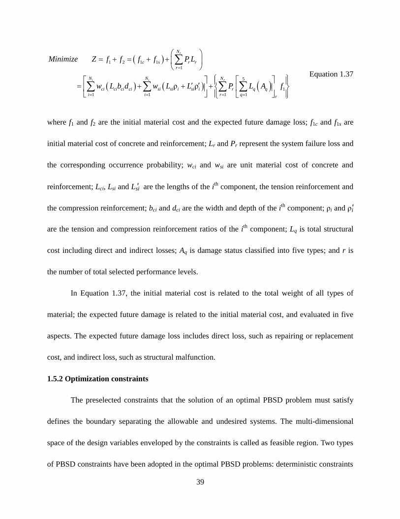
39

1 2 1 1

1

5

1

1 1 1 1

ρ ρ

r

i i r

N

c s r r

r

N N N

ci ci ci ci si si i si i r q q

i i r q r

Minimize Z f f f f P L

w L b d w L L P L A f

Equation 1.37

where f1 and f2 are the initial material cost and the expected future damage loss; f1c and f1s are

initial material cost of concrete and reinforcement; Lr and Pr represent the system failure loss and

the corresponding occurrence probability; wci and wsi are unit material cost of concrete and

reinforcement; Lci, Lsi and L 'si are the lengths of the ith

component, the tension reinforcement and

the compression reinforcement; bci and dci are the width and depth of the ith

component; ρi and ρ'i

are the tension and compression reinforcement ratios of the ith

component; Lq is total structural

cost including direct and indirect losses; Aq is damage status classified into five types; and r is

the number of total selected performance levels.

In Equation 1.37, the initial material cost is related to the total weight of all types of

material; the expected future damage is related to the initial material cost, and evaluated in five

aspects. The expected future damage loss includes direct loss, such as repairing or replacement

cost, and indirect loss, such as structural malfunction.

1.5.2 Optimization constraints

The preselected constraints that the solution of an optimal PBSD problem must satisfy

defines the boundary separating the allowable and undesired systems. The multi-dimensional

space of the design variables enveloped by the constraints is called as feasible region. Two types

of PBSD constraints have been adopted in the optimal PBSD problems: deterministic constraints

40

and probabilistic constraints. The former defines a feasible region, in which the structures with

deterministic design variables satisfy the performance-based constraints. The latter defines a

feasible region, in which a structure with probabilistic distributed design variables satisfies the

allowable failure probability of different performance levels. The structure in this

multi-dimensional feasible region is not defined by the value of design variables, but their mean

values. The values of design variables are changeable during optimal process following a

distribution type with the deterministic mean and variance. Therefore, the structural responses

under the possible values of a design variable are different. The failure probability of the

structure with uncertain variables can be obtained by a statistical analysis.

1.5.2.1 Deterministic constraints

The limit state function of the deterministic constraints used to avoid structural failure

can be expressed by Equation 1.38.

hPG R R X X Equation 1.38

where X is the vector of design variables; R(X)h is the non-linear response of structure with X

under the hth

selected hazard level; [RP] represents the deformation limit of the p

th performance

levels; G(X) defines the limit state function of X for the pth

performance level under the hth

hazard level. The performance level and corresponding hazard level are predefined according to

Figure 1.1. Each combination of a performance level and a hazard level is called a performance

objective. All selected performance objectives shall be achieved.

41

Normally, nonlinear deformation instead of the force or acceleration of structure is

selected as the constraints for an optimal PBSD problem. Two types of non-linear deformation

are considered in optimal PBSD: inter-story drift ratio and plastic hinge rotation, as expressed as:

Equation 1.39

θ θ Equation 1.40

where Δ and [Δ] are inter-story drift ratio of the structure and corresponding limits; θ and [θ] are

plastic hinge rotation of columns or beams and its limits.

1.5.2.2 Probabilistic constraints

Uncertainty exists in external loads, material properties, construction, and numerical

analysis. The failure probability of a structural caused by these uncertainties can be quantified by

structural reliability analysis, which identifies the failure probability of the structure using

models with discrete input variables following certain probability distributions.

The limit state function of the deterministic constraints defined in Equations 1.39 and

1.40 includes inter-story drift, and plastic hinge rotation of beams and columns. A structure fails

when any one of these limit state functions is unsatisfied, that is the structure model shall be

taken as a series system. Therefore, structure failure probability derived from probability analysis

can be defined as Equation 1.41.

P 0 P θ θ βp ph hG

X Equation 1.41

42

where X is the vector of the design variables; G(X) is limit state function of the deterministic

deformation constraint with X; P[ ] is conditional probability; symbol expresses the union of

two condition subsets; Φ( ) is the standard normal distribution function, which has zero mean

and unit variance; β is the reliability index of non-linear deformation of structure.

The probabilistic format of the deformation constraints can be defined as that the failure

probability in limit state function is lower than its limit, as shown in Equation 1.42 or 1.43.

P 0 pG p X Equation 1.42

β β p Equation 1.43

where [PP] is the allowable failure probability of the nonlinear deformation of structure in the p

th

performance level; [βP] is the allowable reliability index of non-linear deformation of structure

under in the pth

performance level.

To date, only SEAOC (1995) proposed the acceptable failure probability of structural in

deferent performance levels, which was based on the study of Paulay and Priestley (1992) and

shown in Table 1.3. In this table, [Pf,a] and [βj,a] are the allowable annual failure probability and

the reliability index; [PfE] and [βj,T] are the allowable failure probability and the reliability index

of period (normally 50 years).

43

Table 1.3 Target annual probabilities of nonperformance recommended by Paulay and Priestley

(1992)

Performance level [Pf,a] [βj,a] [PfE] [βjT]

Operational 0.0200 2.054 0.100 1.276

Life safety 0.0020 2.878 0.010 2.326

Collapse prevention 0.0002 3.540 0.001 3.090

1.5.3 Optimal algorithms

The two major optimization algorithms for PBSD are metaheuristics and optimality

criteria (OC) methods. The metaheuristics method treats the optimal variables of a structure as

the variables of an object in natural world or a social phenomenon, and imitates a searching

mechanism for an optimal design following the natural phenomena or societal laws. The

advantage of this method is that it requires neither explicit expression of the constraints, nor the

explicit formulations of the searching path for the optimal solution. Nevertheless, great

computational effort is required to simulate the searching mechanism.

In contrast, OC method requires much less computational effort, but needs explicit

constraints defined by the optimal variables. The optimal PBSD is then transformed to a

nonlinear programming problem, which can be solved by diverse mathematical methods. The

efficiency of these mathematical methods depends on the path of searching optimal solution.

1.5.3.1 Metaheuristics methods

The metaheuristics methods adopted in the optimal PBSD problems include genetic

algorithm (Liu et al., 2005; Kaveh et al., 2012), ant colony algorithm (Kaveh et al., 2010), neural

networks algorithm (Möller et al., 2009), particle swarm algorithm (Talatahari, 2013; Gholizadeh

44

and Moghadas, 2014), charged system search algorithm (Talatahari et al., 2014), and discrete

gravitational search algorithm (Yazdani et al., 2016). The gravitational search algorithm

employed by Yazdani et al. (2016) is described here to demonstrate how the structure variables

are encoded by the natural objects and how the natural phenomenon is used to search the optimal

solution. Gravitational search algorithm was first proposed by Rashedi et al. (2009) to search

optimal solution based on Newton's law of gravity and the law of motion defined in Equations

1.44 and 1.45.

1 2

2

M MF G

R Equation 1.44

1

1

Fa

M Equation 1.45

where F is the universal gravitation between two objects; G is the gravitational constant; M1 and

M2 are the masses of two objects; R is the interval between the two objects; a1 and M1 are the

acceleration and the mass of the first object.

The gravity law states that the universal gravitation between two objects in the space is

proportional to their masses, and inversely proportional to the square of their interval. The law of

motion indicates that the acceleration of one objective is proportional to the external force

applied on it and inversely proportional to its mass. To apply these natural laws, the gravitational

search algorithm assumed that a space with N dimensions includes finite objects. The location

vector of the ith

object, Xi, is expressed in Equation 1.46.

45

1, , , ,d n

i i i iX x x x Equation 1.46

where xd

i is the position of the ith

object in the dth

dimension. The number of space dimension

shall be equal to the number of the optimal variables Therefore, each position in this space is a

possible solution of optimal PBSD. In the other word, the location of a position in the ith

dimension represents the value of the ith

design variable.

These objects move in the N-dimension space based on the Newton's law of gravity and

the law of motion. Each object experiences universal gravitations from all other objects in the

space, as shown in Figure 1.12. The resultant force, F1, determines the object’s motion direction.

The acceleration of this object is determined by the external force and its own mass. The initial

masses of all objects are identical but modified during the searching process based on a fitness

function. For the objects close to the optimal solution, their masses increase at the current time

Figure 1.12 The combined universal gravitation force and the universal gravitations caused by

the other masses (Rashedi et al., 2009)

46

step, while the masses of other objects decrease simultaneously. With the additional mass, the

object has larger attraction to other objects, and its speed is reduced. Nevertheless, this trend is

opposite for other objects, which are far from the optimal solution. Finally, all the objects will

stop around the heaviest one, which has the ultimate value of fitness function and represents the

optimal design solution. The modified masses of the ith

object at searching time, t, is shown in

Equations 1.47 and 1.48.

1

i

i N

j

j

m tM t

m t

Equation 1.47

i

i

fit t worst tm t

best t worst t

Equation 1.48

where mi(t) and Mi(t) are the inertial and gravitational masses of the ith

object at time t; fiti(t) is

the fitness value of the ith

object at time t; worst(t) and best(t) are the highest and lowest (or

inverse depending on the objective function) fitness value among all objects.

The computational effort of any metaheuristics method is considerably high. For instance,

Kaveh et al. (2010) applied both ant colony optimization algorithm (ACO) and genetic

algorithms (GA) to the optimal PBSD of two plane steel moment frames shown in Figure 1.13.

The time required at each iteration step was almost identical for two algorithms, thus the

computational cost depended only on the required number of iteration. To decrease the design

variables, 27 members in the 3-story frame (Figure 1.13(a)) were unified into five groups, and

47

108 members in the 9-story frame (Figure 1.13(b)) were unified into 13 groups. Thus, this

method does not deliver a global optimal design.

For the 3-story steel moment frame, the required analysis rounds of ACO and GA were

3900 and 6800, respectively. The optimal weight obtained from ACO was 6.79% lighter than

from GA. The standard deviation of the results obtained from the ACO and GA algorithms were

1.701 kips and 3.222 kips, respectively. The 9-story frame was optimized for two cases. For the

(a)

(b)

Figure 1.13 Two steel frame examples in the study of Kaveh et al. (2010): (a) Three-story

four-bay planar steel moment frame; (b) Nine-story five-bay planar steel moment frame

48

first case, both beams and columns were taken as optimal variables. For the second case, only

beams are optimized with predetermined columns. The required analysis rounds for the first case

were respectively 7000 for ACO and 11500 for GA algorithms. For the second case, the needed

analysis rounds were 5600 and 9700 for ACO and GA algorithms, respectively. Therefore,

without a fully automated design process, these metaheuristics methods are difficult to be used in

the engineering practice due to the high computational cost.

1.5.3.2 OC methods

OC method is a type of gradient-based method that determines searching direction and

speed based on the gradient of constraints, which can be explicitly expressed by design variables

based on some simplifications. The key challenge existing in OC method is how to transform a

structural optimization problem with implicit constraints, which cannot be explicitly formulated

by the optimal variables, into a nonlinear programming problem with explicit constraints. The

challenge was tackled by some researchers. Grierson et al. (2006) and Xu et al. (2006) proposed

a performance-based OC method for steel moment frames with a multi-objective function shown

in Equation 1.36. For steel structures, the stiffness and strength of an element are determined by

section characteristics, such as the moment of inertia, I, elastic modulus, S, and plastic modulus,

Z. This OC method expressed all these section characteristics only by section sizes A, as shown

in Equations 1.49 to 1.51.

2

1 2 3I C A C A C Equation 1.49

49

4 5S C A C

Equation 1.50

ςZ S Equation 1.51

where C1 to C5 are constants determined by a regression analysis (Gong, 2003); and ς is a shape

factor depending on the cross-section type.

The allowable values of inter-story drift ratio and roof displacement was well as the

upper and lower bounds of section size were considered as constraints, as shown in Equations

1.52 to 1.54. Equation 1.36 was used to define an objective function. However, the second part

of the multi-objective function in Equation 1.36 and the nonlinear deformation constraints shown

in Equations 1.52 and 1.53 were implicit with respect to A. Therefore, the first-order Taylor

series were used to reformulate the objective function and constraints into Equations 1.55 to 1.58.

The implicit objective function and constraints were formulated by reciprocal sizing variables, x

= 1/A, and sensitivity coefficients of inter-story drift ratio, roof displacement and

ductility-demand, dδ/dxj, dΔ/dxj and df2/dxj. The definition of x can be found in the study by

Schmit and Farshi (1974). The method to calculate the sensitivity coefficients was proposed by

Gong et al. (2005). Therefore, the optimal PBSD problem was transformed to a nonlinear

programming problem with the objective function and constraints explicitly expressed by A.

:δ δ 1,..., ; 1,...,i i

s h sSubject to x i n s n Equation 1.52

1,...,i i

hx i n Equation 1.53

1,...,L U

j j jA A A j n Equation 1.54

50

where δi

s and [δi] are the inter-story drift ratio on the s

th story and its allowable value at the i

th

hazard level; Δi and [Δ

i] are roof displacement and its allowable value at the i

th hazard level; Aj,

[AL

j ] and [AU

j ] are the cross sectional area and its lower- and upper bound values of the jth

component; nh, ns and n are the number of the hazard level, stories and components.

1 2

0

0 2 012 2

1 1max

:

1 ρ

CP

n n

j j j

j jj j

Minimize f x f f

df xL f x x x

W x dx

Equation 1.55

0

00

1

δ: δ δ 1,..., ; 1,...,

insi i

s j j h s

j j

d xSubject to x x x i n s n

dx

Equation 1.56

0

00

1

1,...,

ini i

j j h

j j

d xx x x i n

dx

Equation 1.57

1,...,L U

j j jx x x j n Equation 1.58

where the superscript 0 represents the current design in iteration loop; [xL

j ] and [xU

j ] are the lower

and upper bounds of xj; and CP represents the collapse prevention performance level.

In addition to using Taylor series and sensitivity analysis, Chan and Zou (2004) and Zou

et al. (2005 a and 2005 b) proposed a notable OC method for RC moment frame structures. This

method adopted the virtual work principle to explicitly express the inter-story drift as a function

of the width and depth of all elements, and express the plastic hinge rotation as a function of

tension and compression reinforcement ratios. The optimal PBSD problem, which minimizes the

total material cost, is separated into two optimization phases. The objective of the first phase is to

51

minimize the total concrete cost of the RC frame that needs to satisfy the inter-story drift limit

when the structures behaves elastically under minor earthquakes. In this phase, the section sizes

of all elements are optimized based on the elastic analysis of the structure under the frequent

earthquakes. Equation 1.59 shows the objective function.

1

: ,iN

i i i i i

i

Minimize Z B D w B D

Equation 1.59

where wi is the unit cost of concrete; Bi and Di are the width and the depth of the ith

member; Ni

is the total number of elements.

To explicitly express the elastic inter-story drift by the optimal variables, virtual work

principle is used, as shown in Equation 1.60.

01

ii

n n n n n nNLn X Xj Y Yj Z Zj X Xj Y Yj Z Zj

j

i X Y Z X Y Zi

F f F f F f M m M m M mu dx

EA GA GA GI EI EI

Equation 1.60

where u(n)

j is the virtual work on the jth

story on the nth

mode; Li is the length of the ith

member; E

and G are the Young's modulus and shear modulus of concrete; AX, AY and AZ are the cross

sectional areas perpendicular to local axes X, Y and Z of the element; IX, IY and IZ are torsional

and flexural moments of inertia along axes X, Y and Z of the element; F(n)

X , F(n)

Y , F(n)

Z , M(n)

X , M(n)

Y

and M(n)

Z are the member internal forces and moments; fXj, fYj, fZj, mXj, mYj and mZj are the virtual

member force and moment due to a unit virtual load applied to the building at the location

corresponding to the displacement, uj. The member internal forces and moments could be

52

obtained through structural analysis. Equation 1.60 can be formulated by Bi and Di based on the

three-dimensional elastic theory proposed by Cowper (1996). Therefore, the elastic displacement

can eventually be explicitly expressed by the optimal variables, Bi and Di.

The objective of the second optimization phase is to minimize the total reinforcement

cost in the condition that the RC frame must satisfy the limits of inter-story drift and plastic

hinge rotation under severe earthquakes. In this phase, the reinforcement ratio of each element is

determined based on the nonlinear analysis of the structure subjected to severe earthquakes.

Equation 1.61 shows the objective function.

1

: ρ ,ρ ρ ρiN

i i si si i si ii

i

Minimize Z w L L

Equation 1.61

where wsi is the unit cost of reinforcement; Lsi and L 'si are the length of the tension and the

compression reinforcement of the ith

member; and ρi and ρ 'i are the tension and compression

reinforcement ratios.

Virtual work principle is adopted to explicitly express inter-story drift and plastic hinge

rotation. The virtual work uj on the jth

story derived from a pushover analysis is equal to the sum

of virtual work produced by both the structural members, uj,memb, and by the plastic hinges, uj,hinge,

as shown in Equation 1.62. Because the section sizes have been determined in the first phase,

uj,memb shall be identical to u(n)

j in Equation 1.60. Additionally, based on Zou (2005), uj,hinge can be

expressed by plastic hinge rotations, and the rotation of each element can be explicitly

53

formulated by the optimal variables (ρ and ρ'), as shown in Equations 1.63 and 1.64. Therefore,

the nonlinear deformations can be explicitly expressed by ρ and ρ'.

, ,j j memb j hingeu u u

Equation 1.62

20

,

1 1

θiN

j hinge pjh ph

i h i

u m

Equation 1.63

θθ θ 1

0.1 ρ ,ρ

U

y pU ip pi

u y yi i ii

M M M

M M M

Equation 1.64

where m0

pjh is the virtual moment at the hth

hinge of the ith

member on the jth

story; the subscript i

represents the ith

element; θph is the plastic rotation at the hth

plastic hinge of a member; θU

p is

allowable plastic rotation; M is the applied moment at plastic hinge; My and Mu are the yield and

ultimate moments corresponding to θU

p . My can be explicit expressed by ρ and ρ'.

In addition to the OC methods described above, Li et al. (2010) proposed a hybrid

optimization method that combines the OC method proposed by Chan and Zou (2004) with

genetic algorithm to optimally design RC tall buildings. Hajirasouliha et al. (2012) adopted

Chan's method (2004) to determine section dimensions; however, the objective function is to

minimize the reinforcement weight on each story and the structural damage caused by plastic

hinging.

Note that, the optimal result by OC method may be only a local optimal solution (Huang

et al., 2015). Moreover, the nonlinear deformation of a structure is affected by both strength and

stiffness of the elements. For a RC moment frame, the element flexural stiffness is related to

54

section size, while the element flexural strength is related to both section size and reinforcement

ratio. In addition, the permitted values of structural nonlinear response, such as allowable plastic

hinge rotation determined in Table 1.2, are also a function of the optimal variables, such as

section sizes and reinforcement ratio. Therefore, it is difficult for OC method to obtain the

sensitivity coefficients of multiple variables. Moreover, Zou and Chan (2005) states that for a

statistically indeterminate frame, the explicit constraints of structural responses derived from OC

method are approximate due to the internal force redistribution when an optimal variable is

changed. Therefore, in each iterative round, a complex nonlinear structural analysis is required to

estimate the nonlinear structural response based on the updated variables.

1.6 Research Motivations

This research is motivated by the economic loss due to the conventional force-based

seismic design and the lack of practical optimal PBSD method. Unexpected high economic loss

due to the damage to structural and nonstructural components of buildings occurred during the

recent earthquakes. This was partially caused by the conventional force-based method, which

considers only the life safety performance level (Krawinkler, 1999; Ghobarah, 2001; Sung et al.,

2009). PBSD has been a major focus of earthquake engineering community, because it can better

limit the structural and nonstructural damage under multiple hazard levels (Powell 2008).

PBSD has been widely employed to evaluate the seismic performance of existing

buildings, for which design details such as section size and reinforcement arrangement are

55

already known. However, the force-based design approach is still prevailing for designing new

buildings because of the lack of general procedures of PBSD (Ghobarah, 2001). The current

PBSD method is essentially a trial-and-error method with very high computational cost.

Accordingly, it has been applied mainly to the critical facilities, such as hospital buildings.

The needs to simultaneously design numerous variables, including strength, stiffness and

ductility of all components, and to consider multiple hazard levels call for developing optimal

PBSD. As a result, some optimal PBSD methods described previously were proposed for RC

frames; however, the existing methods have various drawbacks hindering their applications to

the U.S. design practice.

(1) Majority of the available optimal PBSD methods employed inter-story drift to measure

structural performance, while only a few studies (Ganzerli et al., 2000; Zou and Chan, 2005

and Zou et al., 2007) considered the plastic hinge rotation of beams and columns. However,

the plastic hinge rotation of a frame component better describes the local behavior of a RC

frame and has been taken as the only performance measurement in the latest

performance-based evaluation standard, ASCE 41-13 (2014).

(2) As reflected in ASCE 41-13 (2014), the allowable plastic hinge rotation of a beam or a

column is not a constant value; instead, it is a function of the shear stress or axial stress,

which varies during lateral loading. This property was not considered in the existing studies

(Ganzerli et al., 2000; Zou and Chan, 2005 and Zou et al., 2007), which assumed constant

plastic hinge rotation capacity, and would significantly increase the complexity of the

56

optimization problem.

(3) Majority existing optimal PBSDs requires complex algorithms and high computational cost

due to the numerous variables. Therefore, a fully automated design process is needed to

apply these methods. However, the needed computer programs are often not accessible for

practicing engineers.

1.7 Research Objectives

The overall goal of this study is to develop a new optimal PBSD method for multi-story

RC moment frames. The new method is expected to overcome the deficiencies of existing

optimal PBSD methods and can be practically implemented by the U.S. design practice. Specific

objectives include:

Develop a simplified optimal PBSD procedure that incorporates the latest criteria of

structural performance of RC frame buildings and can be practically implemented by design

engineers;

Investigate how much construction cost can be reduced by the proposed method, and how

much the overall strength and stiffness of the optimal design are reduced from those of the

conventional force-based seismic design;

Examine whether the optimal design derived from the proposed method can satisfy the

requirements of the selected performance levels under multiple hazard levels; and

Investigate the influence of the overall strength and stiffness on the structure failure

57

probability and the statistically features of different types of nonlinear deformations.

1.8 Research Methodology and Tasks

Nonlinear pushover analysis is included in the proposed optimal PBSD to estimate the

structural nonlinear deformation under multiple hazard levels. This structural analysis method

permits incorporating various assumptions and simplifications and has low computational cost.

Nonlinear programming is used to determine the optimal solution based on the linear objective

function and the explicit feasible region boundary derived from the proposed method. Nonlinear

dynamic analysis is used to estimate the deformation of the optimal structure, because this

method can provide a more realistic structural response if the hysteretic behavior of structural

components is properly defined (Deierlein et al., 2010). Latin Hypercube sampling method is

adopted to perform the failure probability analysis, because this method can generate reliable

statistical results with comparatively less sampling times.

This study follows the stages shown in Figure 1.14. In the first stage, a new optimal

PBSD method is developed for multi-story RC moment frames. In the second stage, the proposed

optimal PBSD method is applied to a prototype multi-story RC frame building to illustrate the

detailed procedures and to investigate the effects of the proposed method on cost saving. The

third stage examines the seismic performance the optimally designed structure by performing

nonlinear dynamic analyses. The fourth stage investigates the influence of overall strength and

stiffness on the structure failure probability by using Latin Hypercube sampling method.

58

Figure 1.14 Research methodology and procedure of this study

Apply the proposed method on a multi-story RC moment

frame and investigate the cost reduction of the optimal design

Investigate influence on structural failure

probability by overall strength and stiffness

Examine whether the optimal design can satisfy the

performance-based requirement under multiple hazard levels

Develop an optimal PBSD methodology Stage 1

Stage 2

Stage 3

Stage 4

59

CHAPTER 2

OPTIMAL PROFORMANCE-BASED SEISMIC DESIGN METHODOLOGY

2.1 Problem Statements

This study proposed a practical optimal PBSD method to achieve the minimum overall

cost of a multistory RC moment frame, which satisfies the deformation requirements of multiple

performance objectives. In addition, some other seismic design requirements to ensure a desired

failure mode are incorporated to simplify the structural model and reduce the complexity of the

optimization process.

Based on the capacity design philosophy, the expected failure mechanism of the RC

moment frame is a flexural failure, which is a ductile failure mode with observable deflection

and cracking before a dramatic loss of strength. However, the shear failure of RC structural

components is brittle and has little or no warning before a sudden loss of strength. Therefore, the

flexural strength of the elements in a RC moment frame is used as the design basis for

force-controlled actions to make sure that they would not occur. Thus, the optimal methodology

proposed in this study is used to optimize the flexural design. The design methods of the

force-controlled behaviors, such as shear, still follow the procedures of the current seismic

design. In addition, the optimized structure based on the proposed seismic design method shall

also satisfy the gravity design requirements.

60

2.1.1 Objective function

The most widely selected single objective function minimizing total cost of RC moment

frames is adopted in this study. The two types of construction material (concrete and

reinforcement) are taken as the optimal variables. The unit costs of concrete and reinforcement

are associated with volume and weight, respectively. Therefore, the objective function in this

study of the RC moment frame is expressed by Equation 2.1.

c c s sTMinimize C c c W Equation 2.1

where CT = the total cost; Ωc = total concrete volume; Ws = total weight of reinforcements; cc and

cs = unit costs for concrete and steel reinforcement. Normally, the unit cost of different material

includes only the raw material cost without considering the labor cost, such as transportation,

framework, equation, fabrication, and some other aspects. However, the labor cost occupies

about 41% of the overall cost for RC structure (Rwamamara et al., 2010) Therefore, the unit cost

in this study is composed by both raw material cost and labor cost.

2.1.2 Constraints

Because the purpose of optimal PBSD problem is to design a structure satisfying multiple

performance objectives, the constraints shall include the structural behavior limits of multiple

performance objectives. As described previously, the most widely adopted performance-based

limits in PBSD are the nonlinear deformation requirements. Therefore, in this study, the design

code specified nonlinear deformation requirements (inter-story drift ratio and plastic hinge

61

rotation) are adopted to define the performance constraints. Some other seismic design

requirements, such as minimum positive moment at the ends of beams and strength column weak

beam principle, are used to simplify the optimization or as the seismic design constraints.

2.1.2.1 Performance constraints

In this study, both inter-story drift ratio, γ, and plastic hinge rotation angle, θ, are

employed to quantify the structural nonlinear behavior under multiple performance objectives. In

different hazard levels, γ and θ are limited by different allowable values for preselected

performance levels, as shown in Equation 2.2. The hazard levels include at least two of frequent,

occasional, rare and very rare earthquakes, as shown in Figure 1.1.

γ γ , θ θ 1, 2, , p pp pSubject to p P Equation 2.2

where [γ]p and [θ]p are the allowable values for transient γp and θp in the pth

performance level. [γ]

is taken as the global deformation constraint to restrain the damage to nonstructural components,

such as glass curtain walls, and avoid excessive P-delta effects. However, ASCE/SEI 41-13

(2014) has no specification on [γ]; thus, the allowable values of [γ] for RC moment frames in the

different performance levels are determined according to ASCE/SEI 41-06 (2007) shown in

Table 1.1. On the other hand, [θ] is taken as the local deformation constraint to restrain the

damage to structural elements (beams and columns). The allowable values of [θ] for RC moment

beams and columns are determined according to ASCE/SEI 41-13 (2014) shown in Table 1.2.

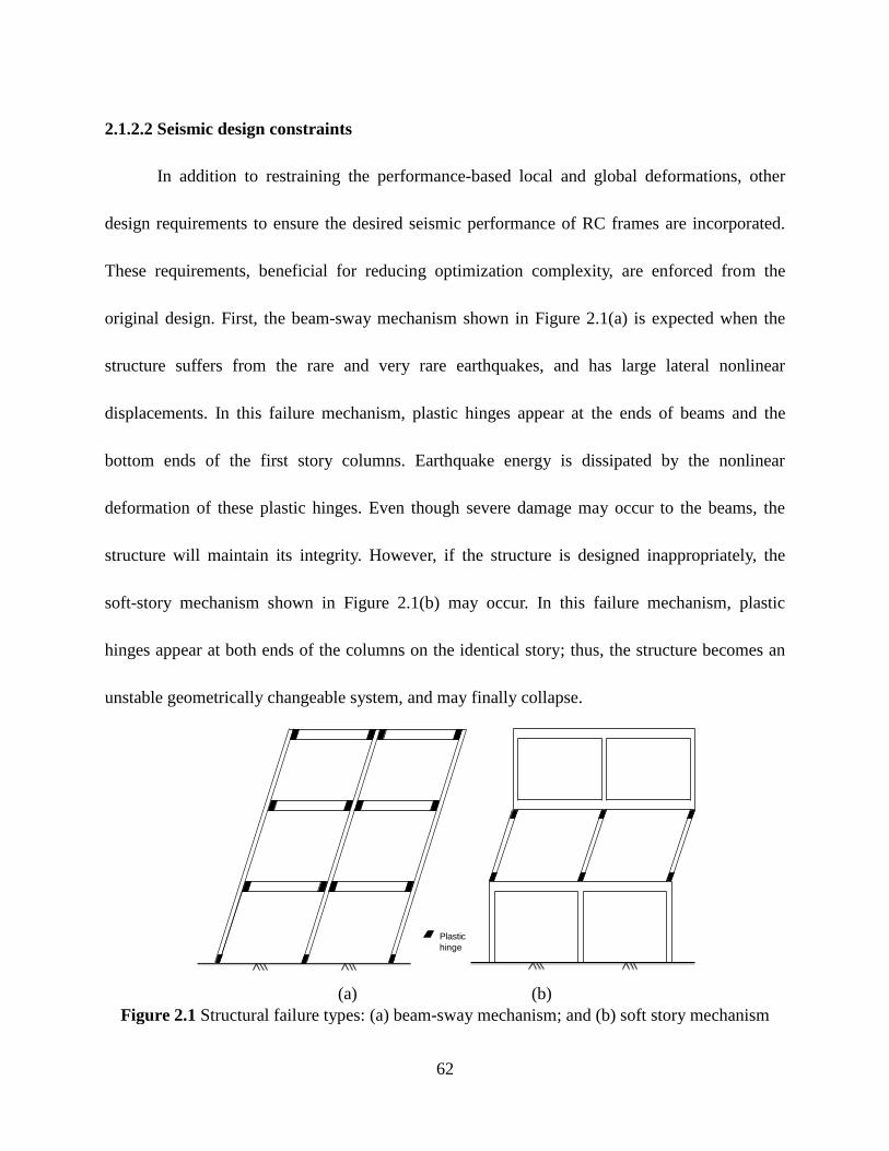
62

2.1.2.2 Seismic design constraints

In addition to restraining the performance-based local and global deformations, other

design requirements to ensure the desired seismic performance of RC frames are incorporated.

These requirements, beneficial for reducing optimization complexity, are enforced from the

original design. First, the beam-sway mechanism shown in Figure 2.1(a) is expected when the

structure suffers from the rare and very rare earthquakes, and has large lateral nonlinear

displacements. In this failure mechanism, plastic hinges appear at the ends of beams and the

bottom ends of the first story columns. Earthquake energy is dissipated by the nonlinear

deformation of these plastic hinges. Even though severe damage may occur to the beams, the

structure will maintain its integrity. However, if the structure is designed inappropriately, the

soft-story mechanism shown in Figure 2.1(b) may occur. In this failure mechanism, plastic

hinges appear at both ends of the columns on the identical story; thus, the structure becomes an

unstable geometrically changeable system, and may finally collapse.

(a) (b)

Figure 2.1 Structural failure types: (a) beam-sway mechanism; and (b) soft story mechanism

Plastic

hinge

63

To avoid the soft-story mechanism, the needed flexural strength of a column is

determined by the maximum bending moment demand this column may experience when the RC

frame is loaded in the nonlinear pushover analysis due to rare or very rare earthquakes.

Additionally, at a beam-column joint, to make sure that the plastic hinges appear at the ends of

beams rather than in the columns, the flexural capacity of the columns shall be larger than that of

the beams. This can be defined as strong column-weak beam behavior. For this purpose, the

method suggested in ACI 318-14 (2014) to determine the flexural strength of columns at a

beam-column joint is adopted in this study, as shown in Equation 2.3.

1.2nc nbM M Equation 2.3

where Mnc and Mnb are the flexural strength of columns and beams framing into a joint,

respectively.

Second, yielding in the first-floor columns is permitted at their bottom ends. However,

prior to the exhaustion of column plastic deformation capacity, the sufficient number of beams

shall have been engaged in developing yielding. The more beam plastic hinges appear, the more

earthquake energy is dissipated and thus less damage will be induced to the columns. In addition,

when a structure suffers the lateral loads caused by earthquakes, the axial force of columns will

increase dramatically. As indicated in Table 1.2, if a column carries a large axial force, its plastic

hinge rotation capacity [θ] is less than that of a beam. Moreover, reduced column size due to

optimization leads to decreased [θ]. Therefore, in this study, the flexural strength at the bottom

64

ends of the first story columns is increased. Following the yielding in the first-floor beams, the

inflection point of a first-floor column moves up and is assumed to be located approximately at

3/4 of column height, as shown in Figure 2.2. The needed flexural strength of a column at the

support, Mnc,2, is then taken as 1.5ΣMnb.

Figure 2.2 Beam-sway mechanism and column flexural strength in the first floor

Third, the code-specified maximum and minimum reinforcement ratios of a section need

to be satisfied. If the reinforcement ratio is higher than the maximum allowable value, the

concrete in compression will fail before the yielding of the tension reinforcement, and an abrupt

failure will occur due to the continuous failure of concrete in compression. The maximum

reinforcement ratio limit ensure sufficient rotation capacity of plastic hinges (Subramanian,

2010). When the reinforcement ratio is lower than the minimum allowable value, an abrupt

failure will occur without warning due to the suddenly increased deformation (McCormac and

Brown, 2015). Therefore, the requirements on ACI 318-14 (2014) about the maximum and

Column bending moment

Inflection

point

Mnb,2Mnb,1

Mnc,2

65

minimum reinforcement ratios of a section is adopted in this study.

Fourth, based on ACI 318-14 (2014), the positive moment strength of a beam at plastic

hinge regions shall be at least half of the negative moment resistance. Therefore, to reduce the

number of the optimal variables, the positive moment strength of a beam can be assumed as half

of the negative moment resistance. Furthermore, other code-specified requirements for the

reinforcement shall be satisfied. For example, ACI 318-14 (2014) requires that both negative and

positive moment strength at any section along the beams shall be at least one-fourth the

maximum moment strength provided at the face of either joint. Moreover, Beam short- and

long-term deflections, shear strength at the beam-column joints, and the shear strength of the

beams and columns should also be satisfied.

2.2 Optimization Methodology

2.2.1 Overview

Figure. 2.3 outlines the optimization procedure developed in this study. In Figure 2.3(a),

the optimal solution is obtained by a nonlinear programming method in this study. The nonlinear

programming problem has a linear objective function and a convex feasible region. The objective

function and constraints in Equations 2.1 and 2.2 incorporates the three major characteristics of

an inelastic system resisting seismic loads (i.e., strength, stiffness and ductility) because Ωc

affects elastic stiffness, Ws is associated with member flexural strength, and γ and θ are related to

ductility. The constraints related to acceptable structural performance define a feasible region for

66

the two decision variables Ωc and Ws. Because the objective function is linear with respect to Ωc

and Ws, the optimal solution (Point A in Figure. 2.3(a)) must be located on the feasible region

boundary and is reached when the objective function becomes tangent to the feasible region.

Figure 2.3 Framework of optimization: (a) optimization in material consumption domain; (b)

stiffness optimization for system with different strengths; (c) MDOF-SDOF transformation; (d)

nonlinear static analysis and determination of roof displacement demands; and (e) N2 method

using inelastic spectra

Despite the simple format of the objective function, several challenges in obtaining the

optimal solution exist. The first challenge is the determination of peak deformation demand

caused by the different levels of seismic hazard. This study intends formulate the peak

deformation demand of a nonlinear RC frame system as a function of its lateral stiffness and

strength. This, however, cannot be achieved by nonlinear time-history analyses. Accordingly,

A

Ws

Ωc

Feasible Region

Objective Function: CT = ccΩc + csWs

γ ≤ [γ], θ ≤ [θ]

α

λ0 1

1

Initial Design

minimized λ at different α

Feasible Region

γ ≤ [γ] θ ≤ [θ]

(a)

(b)

MDOF-SDOF Transformation

Structural Response

MDOF System Equivalent SDOF System

(c)

Optimizations

Hazard 1

Hazard 2 Hazard 3

Inelastic Spectra

D

AV

δ

Push-over Analysis

(d) (e)

Hazard 1

Hazard 2 Hazard 3

Ay

Dy

67

capacity spectrum method, which employs nonlinear static analysis, is adopted to predict the

peak seismic response. The details of applying this method are given later in Section 1.2, and

schematically is shown in Figure 2.3(c).

The second challenge is that the peak nonlinear deformation demand of a RC frame is

affected by not only stiffness but also flexural strength of the beams and columns because the

commonly assumed equal displacement rule may not be applicable. As indicated by Krawinkler

and Seneviratna (1998), the peak lateral displacement of an elastic-perfectly plastic SDOF

system due to ground excitation differs from that of a purely elastic system. The difference is a

function of the fundamental period T, the strength reduction factor R, and the ductility ratio μ.

These properties are correlated through a R-μ-T relationship (Miranda and Bertero, 1994 and

Vidic et al., 1994). It follows that the optimal member size, which controls system elastic

stiffness, cannot be solely determined from a target lateral displacement without considering the

flexural design of members. Accordingly, different from most of the past studies (Zou and Chan,

2005; Xu et al., 2006; Grierson et al., 2006; Li et al. 2010 and Zou et al., 2007) that utilized

nonlinear static analysis, Ωc and Ws are not separately optimized in this study.

The third challenge in obtaining an optimal solution is defining the feasible region

boundary. As indicated in Equations 2.1 and 2.2, the objective function is expressed by material

consumptions Ωc and Ws, whereas the constraints are defined using plastic hinge rotation θ and

optionally by inter-story drift ratio γ. These two sets of variables are correlated by structural

performance predicted by structural analysis. To solve Equations 2.1 and 2.2, either the feasible

68

region boundary is defined by Ωc and Ws or the objective function is transformed as a function of

θ and γ. The former approach is considered. However, the deformation demands in terms of γ

and θ for a multistory RC frame are difficult to be explicitly formulated as a function of Ωc and

Ws. Moreover, as indicated in Tables 1.1, the plastic rotation capacity [θ] of a member is a

function of shear or axial force, which varies during lateral loading, implying that [θ] cannot be

predefined. The coupling effect between plastic hinge rotation capacity and seismic demand

complicates the development of an optimization algorithm and was not considered in the past

studies, which assumed a fixed value of [θ]. A two-stage optimization approach is considered

herein to address these issues. In the first stage, strength-based design procedure is followed to

obtain an original design for the RC frame. Optimization, as shown in Figure. 2.3(b), is then

performed to determine a feasible region boundary defined by discretized pairs of a stiffness

parameter λ and a flexural strength parameter α normalized based on the original design. In the

second stage, the feasible region boundary determined previously in the λ–α domain is converted

into that in the Ωc–Ws domain, from which the optimization problem defined by Equations 2.1

and 2.2 is solved by a nonlinear programming method.

2.2.2 Simplifications

The optimal design of a structural system is ultimately represented by the stiffness and

strength properties of each component. For convenience of formulation, two dimensionless

design variables, a relative flexural stiffness factor denoted as λ and a relative flexural strength

factor denoted as α, are defined for each member. The relative stiffness factor λ is defined as the

69

ratio of section moment of inertia varying during optimization to that determined from the

original design. The relative strength factor α is defined as

0

α n G

n, G

M M

M M

Equation 2.4

where Mn is member flexural strength varying during optimization, Mn,0 is the flexural strength

determined from the original design, and MG is the bending moment caused only by the gravity

loads considered in the seismic design.

λ is optimized for each α using the algorithm described in Section 2.2.3.4. The feasible

region boundary in the λ‒α domain shown in Figure 2.3(b) is determined by connecting the

points with discrete α values and the corresponding minimum λ value. λ = 1 and α = 1

correspond to the sectional stiffness and strength from the original design, respectively. The

parameter λ correlates concrete volume Ωc; the parameter α can be translated into the

consumption of flexural reinforcement Ws when the value of Ωc is determined and indicates the

degree of reducing member flexural strength from that determined from the original design. A

RC frame shall also be designed based on the load combinations purely for gravity loading. A

relative strength factor αG corresponding to gravity design is defined accordingly and taken as

the lower bound of α. αG is evaluated using Equation 2.4 by replacing Mn with MG,0, the bending

moment demand caused by gravity design.

Because many beams and columns exist in a RC frame, the total number of design

70

variables for the entire system far exceeds the two optimal variables Ωc and Ws in Equation 2.1.

To limit the computational cost associated with optimization and enable expressing the feasible

region eventually using the two optimal variables, this study intends to reduce the number of

variables to two as well. For this purpose, it is required that both the ratio of cross-sectional

dimension and the ratio of flexural strength among different members determined from the

original design be maintained during the process searching the minimum λ. In other words, the

relative stiffness factor λ and the relative strength factor α are identical for all the elements at any

step of optimization; thus these two factors can be used as the overall indices measuring stiffness

and strength of the entire structure.

With such a simplification, the additional design requirements described previously,

regarding strong-column/weak-beam and positive flexural strength of a beam section, are not

necessary to be considered as optimization constraints, because they are automatically satisfied

once they have been enforced in the original design. Due to the above simplifications, the design

result based on the proposed approach would not be a global optimal solution mathematically.

However, in a seismic design of RC frame, the member sizes are typically the same in every two

to three stories. Moreover, the beam flexural reinforcement is normally identical on each side of

a beam-column joint. All these features can be incorporated in the original design. Thus, even if

the factors α and λ are used to uniformly modify the original design for simplification purpose,

the optimal design result would be close to a global optimal solution that can reflect design

practice.

71

2.2.3 Determination of feasible region boundary

2.2.3.1 Overview

The key to solving Equations 2.1 and 2.2 is the determination of the feasible region

boundary, which is obtained first in the λ–α domain. A point situated on the feasible region

boundary shown in Figure 2.3(b) can be interpreted as either the minimum λ satisfying

performance criteria at a given α or the minimum α at a given λ. The former definition is

considered to formulate an iterative procedure used to determine the feasible region boundary. A

set of discrete α values ranging from αG to 1 are selected. For each α, the flexural strength of a

member, Mn, is modified from the original design based on Equation 2.4. For the RC frame with

a specific value of α, λ is minimized for each level of earthquake hazard using a procedure

described in Section 2.2.3.4; the controlling value of λ gives the optimal λ for this α. This

procedure is repeated for all selected α values so that a piecewise linear feasible region boundary

is defined in the λ–α domain.

The height and effective depth of a beam are denoted in the following discussions as h

and d, respectively. Their values from the original design are designated as h0 and d0. When

minimizing λ at a given value of the relative strength factor α, the cross-sectional area of frame

members is reduced. Accordingly, in addition to limiting plastic hinge rotation and inter-story

drift ratio, the maximum reinforcement ratio permitted by design codes, ρmax, needs to be

considered as a constraint. The flexural capacity of a beam can be expressed as

72

2ω 1 0 59ωn cM bd f . Equation 2.5

where f 'c is concrete compressive strength; b is beam width; and ω is a tensile reinforcement

index calculated as ω = ρfy / f 'c with fy being the yield strength of reinforcement. Approximating

d/d0 as h/h0, the minimum λ corresponding to ρmax can be derived as

4

30 0 0

1

0 0

ω 1 0 59ωα

ω 1 0 59ω

n, GGmin,

n, G n, max max

M MM .

M M M .

Equation 2.6

where ω0 and ωmax are beam tensile reinforcement index according the original design and ρmax,

respectively. The flexural stiffness of a beam also needs to satisfy the deflection serviceability

requirement under gravity loading. Denoting the minimum relative stiffness needed for this

purpose as λmin,2, the lower bound of λ is then defined as [λ] = maxλmin,1,λmin,2.

The first-stage optimization that minimizes the relative stiffness factor λ at a given

relative strength factor α can then be stated as Equation 2.7. Section 2.2.3.4 presents the detailed

algorithm for solving this optimization problem. Because the flexural strength of a column

interacts with its axial force, which varies during lateral loading, [λ] corresponding to ρmax for

columns cannot be predefined and needs to be checked during optimization. However, the

optimal design for λ should not be affected by ρmax for the columns due to its high permitted

value up to 8% in a design code ACI 318-14 (2014). Once the optimal result of λ becomes

available, the section size of each frame member and thus the total volume of concrete Ωc can be

determined based on those of the original design and the definition of λ. The optimization

73

problem Equation 2.7 is implemented to all selected values of α (αG ≤ α ≤ 1) for each level of

seismic hazard. The data sets of α and its minimum λ constitute the feasible region boundary in

the λ–α domain.

λ

θ θ

θ θ Optinal

λ λ

Minimize

Subject to

Equation 2.7

Each pair of α and its minimum λ provides information regarding the needed flexural

strength and section size, from which flexural designs are conducted for all the beams and

columns. The flexural design may be governed by the minimum reinforcement ratio specified in

design codes; however, this occurs normally at very few locations. Based on the flexural design

of each component, the total weight of reinforcing steel Ws is evaluated. Note each pair of α and

its minimum λ corresponds to a unique pair of Ws and Ωc; hence, the feasible region boundary in

the λ–α domain is transformed into that in the Ws–Ωc domain, where the second stage of

optimization defined by Equations 2.1 and 2.2 can be carried out.

2.2.3.2 Load-deformation response due to modified flexural stiffness

To solve Equation 2.7 at each selected α (αG ≤ α ≤ 1), the peak seismic response of RC

frame in terms of plastic hinge rotation θ and inter-story drift γ need to be determined for each

level of seismic hazard. This is achieved by using capacity spectrum method described in Section

1.2 and summarized in Figures 2.3(c) to 2.3(e). For the RC frame with a specific value of α but

74

without stiffness modification from the original design (i.e., λ = 1), nonlinear static analysis is

conducted. The analysis provides information regarding base shear, roof displacement,

inter-story drift ratio, and plastic hinge rotation. For the structural analysis in this study,

concentrated plasticity model is adopted. This mode simulates the beams and column by line

elements having concentrated plasticity at ends (plastic hinges). The sections outside the plastic

hinge regions are linear elastic with a flexural stiffness taking into account the effects of concrete

cracking. Following gravity loading, lateral loads corresponding to the first vibration mode are

applied. However, if the variation of inertia force distribution due to inelastic response is

considered, an adaptive lateral load pattern (Krawinkler and Seneviratna, 1998; Kalkan and

Kunnath, 2007) accounting for the effects of higher modes and member yielding can be used to

more accurately capture the structural response by means of nonlinear static analyses. The lateral

loading response of the structure with λ = 1 evaluated by a nonlinear static analysis consists of

the generation of a series of plastic hinges. Due to the use of the concentrated plasticity model,

even if the occurrence of each plastic hinging modifies the system stiffness matrix, it remains

identical between two subsequent hinging. Lateral loading causing the jth

plastic hinge is taken as

loading step j and designated by a subscript within parenthesis in the following discussions.

Denoting the system stiffness matrix during loading step j as K(j), the increase in the

displacement of the system Δu(j) and story drift and the increase in lateral load ΔF(j) satisfies ΔF(j)

= K(j) Δu(j). Thus, the total displacement u(j) at the completion of the jth

loading step under load

F(j) is

75

1

1

j

j k kk

u K F Equation 2.8

When the relative strength factor α is fixed and the relative stiffness factor λ is applied

uniformly to all frame members to modify their flexural stiffness, the sequence of plastic hinging

remains unchanged. Accordingly, the stiffness matrix of the modified system during the jth

loading step can be expressed as Kλ

(j) = λK(j). In addition, when the value of α is fixed, modifying

λ has not impact on the load increase ΔFλ

(j) needed to generate a new plastic hinge in the

modified system, that is, ΔFλ

(j) =ΔF(j). Thus, the lateral displacement of the system with modified

stiffness can be derived as

1λ λ λ

1

1

λ

j

j k k jk

u K F u Equation 2.9

Accordingly, under the same lateral load F(j) before causing a collapse mechanism, the

roof displacement δ, inter-story drift ratio γ, and plastic hinge rotation angle θ of the system

modified by λ must satisfy

0 0 0

δ γ θ 1

δ γ θ λ Equation 2.10

where δ0, γ0, and θ0 are the roof displacement, the inter-story drift ratio, and the plastic

rotation angle of the structure without stiffness modification (i.e., λ = 1). Equation 2.10 is of

76

significant convenience for solving the first-stage optimization problem defined in Equation 2.7.

As shown in Figure 2.4, once the base shear vs. roof displacement (V-δ) response of a frame

system at a given value of α but without stiffness reduction (λ = 1) becomes available, it can be

used to directly construct a nonlinear V-δ response for the system with modified flexural stiffness.

Accordingly, there is no need to perform extra structural analyses during the process of searching

for the minimum λ for the structure at the selected α. Thus, the total number of pushover

analyses needed to complete the proposed optimal seismic design is identical to the number of

discretized α values (αG ≤ α ≤ 1) chosen to define a feasible region boundary.

Figure 2.4 Constructing based shear vs. roof displacement response based on nonlinear static

analysis result of the structure without stiffness modification (λ = 1)

2.2.3.3 Determination of minimum stiffness at given flexural strength

For each relative strength factor α (αG ≤ α ≤ 1), the application of capacity spectrum

Roof Displacement δ

Ba

se

Sh

ea

r V V – δ response of initial structure

V – δ response of structure with

reduced stiffness

δ0

δλ= δ0/λ

K(1)

λK(1)

New plastic hinge appears

λK(2)

K(2)

77

method described in Section 1.2 estimates the peak deformation demands. If the limiting values

([θ] and [γ]) are not exceeded under any seismic hazard, the relative stiffness factor λ is

optimized by reducing member section size until one of the constraints in Equation 2.7 controls.

When the section size decreases, reinforcement ratio increases, because the flexural strength of

any element is unchanged. The beam shear stress tends to increase due to reduced section size.

Therefore, the increase of both reinforcement ratio and shear stress result in decreased beam

plastic hinge rotation capacity [θ], as indicated in Table 1.2. Because of the interaction between λ

and [θ], an iterative approach is employed to search for the minimum λ.

A superscript is used for the variables to denote iteration step. The iterations,

schematically illustrated in Figure 2.5, start from λ(0)

= 1, The capacity spectrum method is

applied to evaluate effective period T(0)

and peak displacement D(0)

max of the equivalent SDOF

system as well as story drift ratio γ(0)

and plastic rotation angle θ(0)

at the peak roof displacement

δ(0)

max of the MDOF system. As stated previously and shown in Figure 2.4, at the same value of α,

the based shear vs. roof displacement (V-δ) response for different values of λ can be determined

directly from that of the structure without stiffness modification (λ = 1). It follows that the

idealized bilinear capacity curve for λ(0)

= 1 can be used to construct new bilinear capacity curves

for λ(i)

< 1 (i ≥ 1) in the subsequent iterations. Because member flexural strengths are not

changed, the yield acceleration Ay for the capacity curves associated with different λ values can

be approximated to be identical, as shown in Figure 2.5.

78

Figure 2.5 Effects of modifying relative stiffness factor λ on capacity and demand curves

Between two subsequent plastic hinging in the structure under increasing lateral

deformation, the inter-story drift ratio γ and plastic hinge rotation θ at different locations increase

linearly but at different rates. If neither θ nor γ reaches the allowable value during the previous

iteration step i-1, a parameter η(i)

, defined in Equation 2.11 based on the deformation properties

given in Equation 2.10, is considered to determine the relative stiffness factor λ(i)

for the next

iteration step i. The term related to γ in Equation 2.11 shall be removed if only plastic rotation θ

is used to define optimization constraints in Equation 2.2. The parameter η(i)

is used to control

the iteration speed and determine when the iteration stops. If the absolute value of |η(i)

‒ 1| is less

than a valve v*, then either γ or θ becomes sufficiently close to its limit; thus the iteration stops

and the minimum λ is obtained. The lower bound stiffness parameter [λ] also needs to be

considered. λ(i)

defined by Equation 2.12 is used in step i to uniformly reduce the section

stiffness of the frame members.

A

λ(0) λ(i)

Ay

D(0)max D(i)

max D

Demand Curve

(λ(0) = 1)

Demand Curve

(λ(0) < 1)

79

1

1 1

θ γη

θ γ

i

i

i iMin

Equation 2.11

1

1

λ 1λ λ

ηη

ii

iim

m

Equation 2.12

Once λ(i)

is determined, a new bilinear capacity curve in the equivalent SDOF system is

created. Because λ(i)

uniformly modifies member flexural stiffness in the MDOF system, it can

be approximated that λ(i)

equally affects the lateral stiffness of the equivalent SDOF system. Its

effective period is then determined as T(i)

= T(0)

/(λ(i)

)0.5

, because the equivalent mass is

predominated by the mass of slab and can be assumed as unchanged. As shown in Figure 2.5,

due to decreased system stiffness, the demand curve shifts to the right side, resulting in an

increased spectral displacement. Equation 2.13 can be derived from Equation 2.10 and used to

determine the spectral displacement D(i)

max, story drift γ(i)

, and plastic hinge rotation θ(i)

of the

modified structure in iteration step i.

0 0 0 0

γ θ 1 μ

γ θ λ μ

i i i i

max

i

max

D

D

Equation 2.13

where μ(i)

is determined from the R-μ-T relationship. The strength reduction factor R(i)

needed to

apply the R-μ-T relationship at step i is

80

i

i ae

y

SR

A Equation 2.14

where S(i)

ae is the elastic spectral acceleration for the structure having an effective period of T(i)

.

Iterations with different values of λ are performed until one of the optimization variables

in Equation 2.7 reaches a limit. Reducing λ increases both γ and θ; meanwhile, [γ] is unchanged

and [θ] is reduced due to the increased reinforcement ratio and increased shear stress.

Accordingly, the peak deformation demands in terms of γ and θ gradually approach the limiting

values after each iteration step and a converged result can be obtained.

The minimum relative stiffness factor λ shall be the maximum one among all the relative

stiffness factors derived from different selected performance objectives. The feasible region

boundary in λ‒α domain can be derived by repeating the process of searching minimum λ for

different discretized α values. Then the points on this boundary in the λ‒α domain is transform to

those in the Ωc‒Ws domain. Based on λ and the section sizes of the beams and columns of the

structure without stiffness modification (λ = 1), the element flexural stiffness and section sizes of

the structure modified by λ can be obtained. The total concrete volume Ωc can be derived

accordingly. Because the relative strength factor α is unchanged, the flexural strength of the

beams and columns of the structure without stiffness modification can be used to calculate the

needed reinforcement areas of the elements for the modified structure based on the determined

section sizes. The total reinforcement weight Ws can be accordingly derived.

81

2.3 Optimal Design Procedures

The procedure of the proposed optimal PBSD approach is summarized as follows:

Step 1: A force-based seismic design satisfying the requirements given in Section 2.1.2.2

is conducted to determine the needed flexural strengths of all members. The initial design results

(λ = 1 and α = 1) are subjected to optimization.

Step 2: A series of relative strength factors (αG ≤ α < 1) are selected. For each α, the

member flexural strengths in the initial design are uniformly reduced and Steps 3 and 4 are

implemented. The ratio of section dimension and the ratio of flexural strength among different

members are maintained throughout optimization.

Step 3: For a specific α, the relative stiffness factor is set as λ = 1 and a nonlinear static

analysis is conducted. The considered seismic hazards are defined using elastic spectral

accelerations. Capacity spectrum method is then applied to determine the peak seismic

deformation demands at different seismic hazards for the structure with λ = 1.

Step 4: For the structure with the α value considered in Step 3, the relative stiffness factor

λ is optimized by solving Equation 2.7 using the numerical approach presented in Section

2.2.3.3.

Step 5: Based on the pairs of α and optimized λ determined from the previous steps, a

feasible region is defined in the λ–α domain. For each pair of α and optimized λ, section flexural

design is conducted and the total material consumptions Ωc and Ws are evaluated. The feasible

region in the λ–α domain is then accordingly converted into that in the Ωc–Ws domain.

82

Step 6: The Ωc and Ws that minimize total cost are determined by solving Equations 2.1

and 2.2. The values of λ and α corresponding the optimal Ωc and Ws provide information

regarding the optimal section size and flexural reinforcement design of each member. Finally, the

design code requirement for minimum flexural reinforcement ratio is implemented..

Figure 2.6 shows the flow of the optimal PBSD method proposed in this study

corresponding to the steps above.

83

Figure 2.6 Flow of the optimal PBSD method proposed in this study

START

Perform the initial seismic design (α=1, λ=1)

based on the conventional force-based method

θp=[θ] por

γp=[γ] p

Yes

No

STOP

Flexural design of beams and columns based

on the optimal solution and code requirements θ means the plastic hinge rotation;

γ means the inter-story drift ratio;

p means one performance objective;

P means the total number of the

selected performance objectives

Perform the nonlinear pushover analysis, and estimate

γ p and θ p based on the capacity spectrum method (p=1)

Select discrete αi (1 > αi >αG), and determine the flexural

strength of all the elements corresponding to (α=αi, λ=1)

Perform the gravity-

load design for αG

p=Pp=p+1No

Yes

Determine and record the minimum

λ for αi based on Equation 2.30

Modify based on Equation

2.28, and modify γ p and θ p

based on Equation 2.21

λ(i)

p

αi =αG

Yes

αi = αi+1

No

Estimate λ* based

on Equation 2.26

Use all the pairs of αi and the corresponding minimum λ to

establish the feasible region boundary in the λ–α domain

Transform the feasible region boundary

from the λ–α domain to the Ωc–Ws domain

Solve the nonlinear programming problem with a

linear objective and explicit feasible region boundary

Step 1

Step 2

Step 4

Step 5

Step 6

Step 3

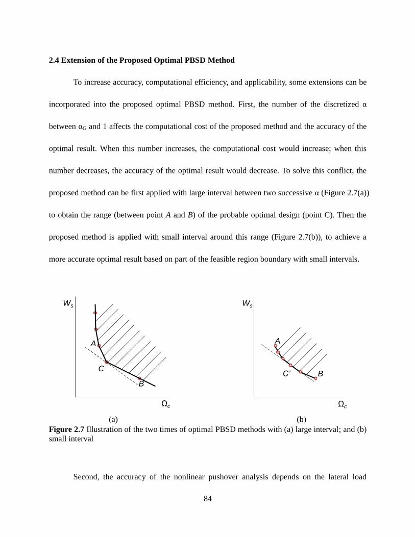
84

2.4 Extension of the Proposed Optimal PBSD Method

To increase accuracy, computational efficiency, and applicability, some extensions can be

incorporated into the proposed optimal PBSD method. First, the number of the discretized α

between αG and 1 affects the computational cost of the proposed method and the accuracy of the

optimal result. When this number increases, the computational cost would increase; when this

number decreases, the accuracy of the optimal result would decrease. To solve this conflict, the

proposed method can be first applied with large interval between two successive α (Figure 2.7(a))

to obtain the range (between point A and B) of the probable optimal design (point C). Then the

proposed method is applied with small interval around this range (Figure 2.7(b)), to achieve a

more accurate optimal result based on part of the feasible region boundary with small intervals.

(a) (b)

Figure 2.7 Illustration of the two times of optimal PBSD methods with (a) large interval; and (b)

small interval

Second, the accuracy of the nonlinear pushover analysis depends on the lateral load

B

Ωc

Ws

C’

Ωc

Ws

A

B

A

C

85

pattern, which simulates the total inertial forces of each story caused by ground acceleration.

However, the inertial force distribution pattern along the height of the structure keeps changing

after the member yielding (Krawinkler and Seneviratna, 1998; Kalkan and Kunnath, 2007), and

the effect of higher modes increases accordingly. Therefore, an adaptive lateral load pattern can

be used by assuming the lateral load pattern is proportional to either the story drift pattern of the

structure (Fajfar and Fischinger, 1988) or to the story shear pattern (Bracci et al. 1997).

2.5 Uniqueness of Proposed Optimal PBSD Method

To compare the optimal strategies of the proposed method with the two-step method

proposed by Zou and Chan (2005), the searching paths of these methods are demonstrated on the

coordinate system defined by total concrete volume Ωc and total reinforcement weight Ws, shown

in Figure 2.8. Figure 2.8(a) illustrates the searching paths of the two-step OC or hybrid

OC‒metaheuristics optimal methods, such as the work by Zou and Chan (2005), Hajirasouliha et

al. (2012), and Li et al. (2010). These methods first optimize the concrete consumption based on

the performance constraints for occasional earthquake by reducing Ωc, then optimize the

reinforcement consumption by reducing Ws based on constraints for rare and very rare

earthquakes. The computational cost of this strategy is reduced compared with the first one;

however, this method essentially assumes that (1) no nonlinear deformation appears on the

structure under the occasional earthquake; thus the deformation constraint of the first step is a

straight line perpendicular to the Ωc axis; (2) the optimal design (point A in Figure 2.8(b)) is

86

controlled by the deformation constraint of the occasional earthquake (corresponding to IO

performance level). However, in ASCE 41-13 (2014) nonlinear deformation is allowed in the RC

moment frame under occasional earthquake. In addition, no evidence has been proved that the

optimal result is controlled by the constraint of the occasional earthquake, such as point A' in

Figure 2.8(a).

Figure 2.8 Comparison of the searching method of different optimal algorithms: (a) OC method

proposed by Zou and Chan (2005); (b) and (c) optimal algorithm proposed in this study

Figures 2.8(b) and 2.8(c) demonstrates the searching paths of the two-step optimal

Ws

Ωc0

Initial design

Local optimal result

Feasible region

Optimal path

Objective function

Final optimal result

Feasible region

boundary

Ws

Ωc0

Min Ωc

Min Ws

Min Ωc+WsIO LS CP

(a)

0

IO LS CP

α

λ

Min Ωc+Ws

IO, LS, and CP

(b) (c)

A’

A

87

method proposed in this study. This method first adopts all the constraints of different hazard

levels to determine the feasible region boundary in λ–α domain, then transforms it into Ωc–Ws

domain for optimal solution by nonlinear programming method. Several innovations of the

proposed optimal PBSD method are that: (1) this method reduces numerous optimal variables

(section size and reinforcement area of all elements) into only two variables (λ and α) based on

some rational simplifications of construction and seismic design. Accordingly, the complexity of

the optimization and the computational cost is highly reduced than the current optimal PBSD

methods. (2) instead of repetitively applying complex nonlinear structural analyses, an explicit

relationship is suggested to express the nonlinear deformation (plastic hinge rotation and

inter-story drift) based on λ and single pushover analysis results, if the flexural strength of all

elements remain unchanged. This explicit expression relates nonlinear deformation to λ and α,

which can be transformed to Ωc and Ws; thus the optimal variables Ωc and Ws in the objective

function (Equation 2.1) can be used to formulate the nonlinear constraints (Equation 2.2). In

addition, mathematical iteration is used to search the minimum λ for each α, instead of iterative

method using complex nonlinear structural analyses. (3) the two-step method first determines the

feasible region boundary by simultaneously using the constraints of multiple hazard levels;

therefore, the possible inaccuracy described in Figure 2.8(c) is avoided. In addition, the two-step

method separately using constraints and objective function at each step to reduce the complexity

of the optimal process.

88

CHAPTER 3

IMPLEMENTATION OF THE PROPOSED OPTIMAL PBSD METHOD AND

EXAMINATION OF THE OPTIMAL DESIGN

3.1 Implementation of the Proposed Optimal PBSD Method

3.1.1 Initial design of the original RC frame structure

The suggested optimal PBSD approach is applied to a six-story prototype RC moment

frame building shown in Figure 3.1. The building, with a story height of 12 ft and a span of 30 in

either direction, is located on a soft rock site in southern California, where the mapped

short-period and 1-sec spectral accelerations for 5% critical damping for the hazard level with

2%/50 year probability of exceedance are Ss = 1.50g and S1 = 0.60g, respectively. Concrete

compressive strength is assumed as 5000 psi and reinforcement yield strength as 60 ksi. The

floors consist of 8 in. thick two-way slabs. A dead load of DL = 117 psf and a live load of LL =

20 psf act on the roof, whereas these values are 120 psf and 50 psf for all other floors.

Modal response spectrum analysis is used to perform a strength-based design. Based on

requirements of ASCE 7-10 (2010), two vibration modes are considered to obtain design base

shear and lateral loads. To meet the 2% inter-story drift limit, the section size of the beams is

chosen as 22 in. × 32 in. for the 1st to the 3

rd floors and 20 in. × 28 in. for the 4

th to the 6

th floors,

and the section size of the columns as 29 in. × 29 in. for the 1st to the 3

rd floors and 24 in. × 24 in.

for the 4th

to the 6th

floors. The flexural design of members follows the seismic design provisions

in ACI 318-14 (2014) as well as the additional design requirements described in Section 2.1.2.2.

89

Table 3.1 gives the needed negative and positive moment resistances for the beams and columns

of an interior frame of the original design.

(a)

(b)

Figure 3.1 Prototype RC frame building: (a) floor plan; and (b) elevation plan

30×4=120 ft30×

4=

12

0 ft

30×4=120 ft

12×

6=

72

ft

90

Table 3.1 Flexural capacity of the elements in the original structure (unit: kip-in.)

Floor

Beam Column

External Internal External Internal

M ‒ M

+ M

‒ M

+

Roof 3682 2974 4505 2974 4204 5001

5 5240 2974 5532 2974 5001 6399

4 5647 2974 6054 3027 5505 7798

3 6762 4310 7107 4310 9603 13400

2 6992 4310 7222 4310 10400 15002

1 6514 4310 6868 4310 11099 17002

3.1.2 Finite element model

Because the proposed optimal PBSD method is based on the nonlinear static analysis

results of a two-dimensional (2D) frame, the interior RC moment frames designed with and

without optimal PBSD are simulated using the software Open System for Earthquake

Engineering Simulation (OpenSees 2017). The structural elements (beams and columns) are

modeled using displacement-based line elements with zero-length plastic hinges at the element

ends as shown in Figure 3.2(a). Each element contains two types of regions along its length:

zero-length plastic hinge at element ends and elastic portion between the plastic hinges (Figure

3.2(b)). The nonlinear model suggested by Ibarra et al. (2005) is used to define the backbone

moment-rotation of the zero-length plastic hinges (Figure 3.2(c)). The parameters of the

backbone curves are defined based on ASCE 41-13 (2014). The elastic flexural stiffness of the

beams and columns are defined as 30% and 50% of uncracked sectional stiffness, respectively.

The gravity loads applied on the beams include factored dead load plus 50% of design live load.

91

Figure 3.2 Illustration of (a) location of the zero-length plastic hinge elements; (b) concentrated

plasticity model of one column; and (c) moment-rotation backbone curve of the plastic hinge

suggested byLignos and Krawinkler (2012)

The member flexural stiffness Kele is composed by the stiffness of the line element Kbc

and the stiffness of the zero-length plastic hinges Kph, which are needed to be defined for the

nonlinear model used in OpenSees. As a series system, Kele is expressed as

(a)

(b)

(c)

Gravity loads

Equivalentgravity loads

Seismic

loads

92

Equation 3.1

Kele shall be distributed appropriately to avoid the numerical instability problem caused

by concentrating of all the stiffness on either the line element or the plastic hinges. Therefore, a

method suggested by Ibarra and Krawinkler (2005) is adopted. This model defines the flexural

stiffness of the plastic hinges is n times of the line element. Therefore, the value of Kbc and Kph

can be expressed by Kele using Equation 3.2. Ibarra and Krawinkler (2005) suggested that the

value of n shall be much larger than 1. However, due to the lack of further explanation, a series

of numerical experiments are performed on the models with different n values (10, 100, and

1000). No difference is found among the results of these experiments; thus, the value of n is

defined as 10 in this study.

Equation 3.2

DL of the beams and columns is normally assumed to be distributed along their

longitudinal directions. Nevertheless, the DL of slabs, the superimposed DL and LL are

uniformly applied on the top surfaces of slabs. As a results, the gravity loads transferred from the

slabs to the beams (Figure 3.3(a)) are not uniformly distributed on the beams; instead, the load

distribution should be linear, as shown in Figure 3.3(b). However, OpenSees cannot apply this

linearly increased load along elements. Thus, these loads are transformed equivalently to five

1

1 1

bc ph

ele

bc ph

bc ph

K KK

K K

K K

1

1bc ele ph ele

nK K K n K

n

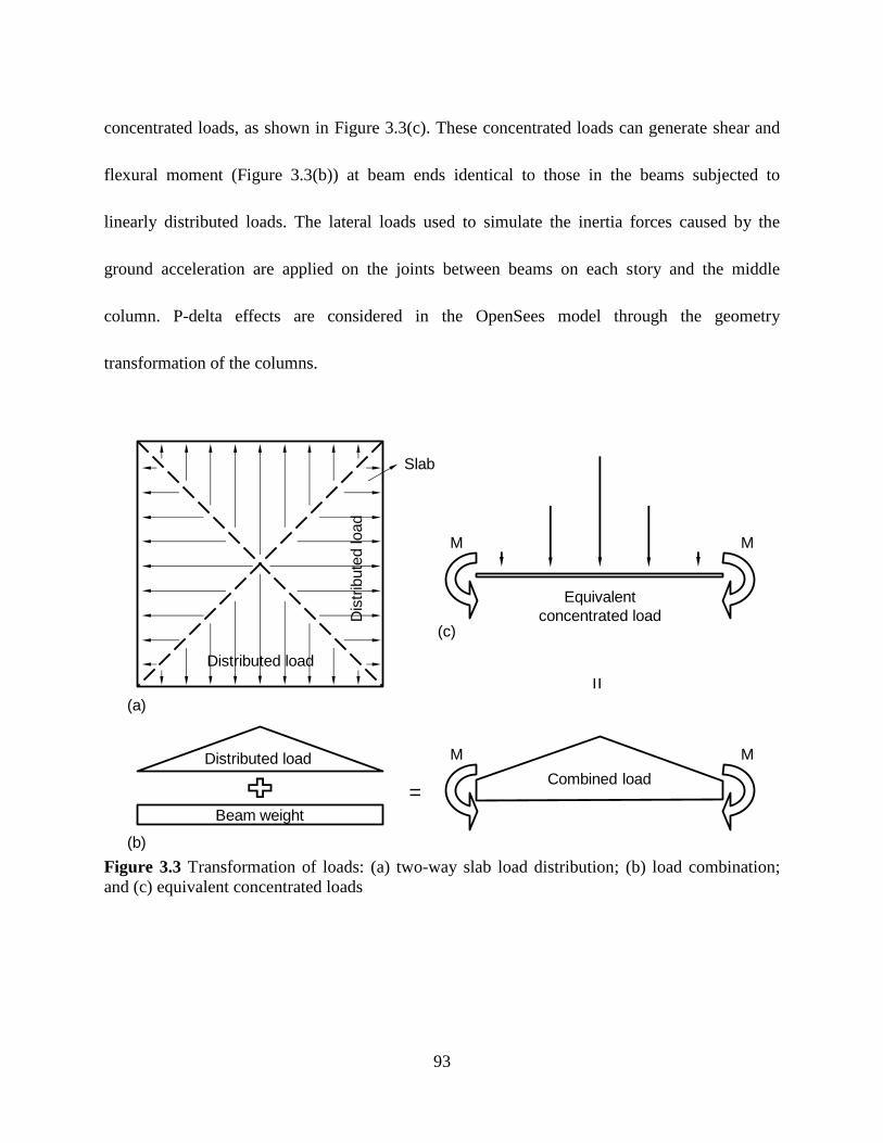
93

concentrated loads, as shown in Figure 3.3(c). These concentrated loads can generate shear and

flexural moment (Figure 3.3(b)) at beam ends identical to those in the beams subjected to

linearly distributed loads. The lateral loads used to simulate the inertia forces caused by the

ground acceleration are applied on the joints between beams on each story and the middle

column. P-delta effects are considered in the OpenSees model through the geometry

transformation of the columns.

Figure 3.3 Transformation of loads: (a) two-way slab load distribution; (b) load combination;

and (c) equivalent concentrated loads

Distributed load

Beam weight

Combined load

Equivalent

concentrated load

M M

M M

(a)

(b)

(c)

Distributed load

Dis

trib

ute

d load

Slab

=

=

94

3.1.3 Optimization

3.1.3.1 Feasible region boundary in λ‒α domain

To apply the capacity spectrum method during optimization, Sae needs to be determined

for different levels of seismic hazard. Based on ASCE 7-05 (2005), Sae is formulated as a

function of mapped spectral accelerations at short period (Ss) and 1-sec periods (S1) as well as the

site condition. Ss and S1 are 1.50g and 0.60g for very rare earthquakes (2%/50 years events) and

1.00g and 0.377g for rare earthquakes (10%/50-yrs events), respectively. Ss and S1 for occasional

earthquakes (50%/50 years events) unavailable from the seismic maps can be calculated based

on ASCE 41-06 (2007) by Equation 3.3.

Equation 3.3

where Si is the spectral response acceleration parameter at the desired probability of exceedance

(“i”=“S” for short period, or “i”=“1” for 1-sec period); Si10/50 is the spectral response acceleration

parameter at a 10%/50-year exceedance rate (“i”=“S” for short period, or “i”=“1” for 1-sec

period); the value of n is 0.29 for the earthquakes in California. Based on this equation and a

mean return period of 72 years, Ss and S1 are evaluated as 0.436g and 0.164g for occasional

earthquakes. R-μ-T relationship suggested by Vidic et al. (1994), which is expressed by Equation

1.6 to 1.9 is employed. The peak ground motion acceleration (ag) and velocity (vg) at a specified

seismic hazard, needed for applying the R-μ-T relationship, are determined based on the mapped

10/50475

n

Ri i

PS S

95

data provided by U.S. Geological Survey, and listed in Table 3.2.

Table 3.2 Peak ground motion acceleration and velocity for three hazard levels

Three hazard levels

2%/50 year 10%/50 year 50%/50 year

ag (cm/s2) 461.47 244.94 106.79

vg (cm/s) 43.24 22.56 9.62

The optimization procedure described previously is followed. Eight values for the

relative strength factor, including α = αG = 0.28 and α = 0.4 to 1 at an interval of 0.1, are selected

to determine the feasible region boundary in the λ‒α domain. For each α, the optimal relative

stiffness factor λ is evaluated for the three considered levels of seismic hazard and shown in

Figure 3.4. For comparison purpose, this figure shows the optimal λ values evaluated based on

the individual types of constraint (i.e., plastic hinge ration limit, drift limit, and minimum relative

Figure 3.4 Feasible region of the six-story four-span RC moment frame in λ–α domain

0.2

0.3

0.4

0.5

0.6

0.7

0.8

0.9

1

1.1

0.1 0.2 0.3 0.4 0.5 0.6 0.7 0.8 0.9 1 1.1

Re

lative

Str

en

gth

Fa

cto

r α

Relative Stiffness Factor λ

Maximum reinforcement ratio

Plastic hinge rotation (2%/50 yrs)

Inter-story drift (2%/50 yrs)





96

stiffness factor) for each seismic hazard level. It is seen that λ is approximately linear with

respect to α except for inter-story drift due to occasional earthquakes. In general, λ decreases

with increased α. In other words, the flexural strength and stiffness of the structural members are

not independent to each other in terms of the optimization results.

As seen in Figure 3.4, if no strength reduction is considered (α = 1), inter-story drift limit

for LS under rare earthquakes governs the optimal relative stiffness factor λ. In this case, λ is

determined as 0.51, leading to a 29% reduction in cross-sectional area. If inter-story drift is not

taken as a constraint, the optimal relative stiffness factor becomes λ = 0.40, controlled almost

identically by plastic hinge rotation limit for LS under rare earthquakes or inter-story drift limit

for IO under occasional earthquakes.

The pairs of selected α and the governing optimal λ based on all constraints constitute the

feasible region boundary in the α–λ domain shown in Figure 3.4. The optimal λ is controlled by

either inter-story drift ratio limit for Life Safety (LS) under rare earthquakes if 0.5 ≤ α ≤ 1 or

plastic-hinge rotation limit for Immediate Occupancy (IO) under occasional earthquakes if α <

0.5. Note that the inter-story drift limit under occasional earthquake is far from controlling the

feasible region boundary. This result is remarkably different from some existing optimal PBSD

approaches for RC frames (Zou and Chan, 2005; Li et al., 2010; and Zou et al., 2007), which

optimized section size based only on the inter-story 0.2 drift limit under minor earthquakes.

Moreover, deformation limits defined for CP under very rare earthquakes also have no impact on

the feasible region boundary.

97

3.1.3.2 Feasible region boundary in Ωc‒Ws domain and optimal solution

For each pair of α and λ on the feasible region boundary shown in Fig. 3.3, the needed

section size is determined, and the flexural designs of beams and columns are conducted. Then,

the total weight of steel reinforcement Ws and total concrete volume Ωc for all the beams

(including those in the transverse direction) and the columns located between the slab center

lines enclosing an interior frame are evaluated. Figure 3.5 shows the new feasible region

boundary defined in the Ωc–Ws domain. To define the objective function expressed in Equation

2.1, the unit cost of concrete and steel reinforcement, cc and cs, are calculated based on the

construction cost data published by the BNi Building News (2015) and RS Means (2015) and

listed in Table 3.3. cc and cs consider both material and labor cost; cc also includes formwork cost

defined based on four uses. For comparison purpose, Table 3.3 also provides the unit costs

Figure 3.5 Feasible region boundary and optimal solutions in Ωc–Ws domain

15

16

17

18

19

20

220 230 240 250 260 270 280 290 300

To

tal W

eig

ht o

f L

on

gitu

din

al R

ein

forc

em

en

t W

s

(to

n)

Total Volumn of Concrete Ωc (cubic yard)

Boundary of feasible region

Objective function (considering both material and labor costs)

Objective function (considering only material cost)

(α = 0.70 , λ = 0.55)

(α = 0.60 , λ = 0.57)

98

considering only the material cost.

Table 3.3 Unit cost of material only and combined material and labor cost

Material Cost Only Material Cost and Labor Cost

unit cost of concrete (cc) unit cost of steel

reinforcement (cs) unit cost of concrete (cc)

unit cost of steel

reinforcement (cs)

$119/C.Y. $940/ton $352/C.Y. $1624/ton

The solid line in Figure 3.5 shows the object function. The tangent point between the

objective function and feasible region gives the optimal solution in terms of Ws and Ωc, which

correspond to α = 0.70 and λ = 0.55. The optimal design leads to a 30% reduction in needed

flexural strength and a 26% reduction in cross-sectional area from the initial strength-based

design. For comparison purpose, the dashed line in Figure 3.5 represents the object function

considering only material cost, which is generally used by existing optimal PBSD methods

(Fragiadakis and Papadrakakis, 2008; Grierson et al., 2006; and Xu et al., 2006). The optimal

solution is α = 0.60 and λ = 0.57. The optimal design corresponds to a 40% reduction in seismic

design loads and a 25% reduction in section area from the initial strength-based design.

Figure 3.6 shows the capacity curve for the optimized structure (λ = 0.55, α = 0.70) in the

equivalent SDOF system and the demand curves (inelastic displacement–acceleration spectra)

for the three levels of considered earthquake hazard. As shown by the capacity curve derived

from nonlinear static analysis, the structure experiences little strength degradation after reaching

the peak load. Moreover, the demand curve for occasional earthquakes intersects the first branch

99

of the idealized bilinear capacity curve, indicating an overall elastic behavior of the optimized

structure under occasional earthquakes.

Figure 3.6 Application of the capacity spectrum method to determine the seismic deformation

demands of occasional, rare, and very rare earthquakes

3.1.3.3 Construction cost reduction due to optimal design

The costs of the interior frame based on the initial design and the cost based on the

optimal design are evaluated and compared in Table 3.4. The optimal design reduces the needed

flexural strengths of the beams and columns by 30%. However, because of the 14% decrease in

section size, the cost of flexural reinforcement in the optimal design is reduced by only 5%.

Major cost saving is contributed by the significantly decreased concrete consumption and the

corresponding labor cost. The transverse reinforcement needed for shear and confinement in the

beams and columns are designed based on ACI 318-14 (2014). The section size reduction

0

0.04

0.08

0.12

0.16

0.2

0 4 8 12 16 20

Sa

(g)

Sd (in.)

50%/50 years 10%/50 years

Inelastic Sd‒Sa Spectra

Idealized Capacity Spectrum

2%/50 years

100

decreases the length of the transverse reinforcement but increases the number of needed

transverse reinforcements. Therefore, the total weight of transverse reinforcement is almost

identical between the optimal and original structures.

Table 3.4 Comparison of cost for the initial and optimal designs

Original design

($)

Optimal Design

($)

Cost Reduction

(%)

Concrete 37,497 27,977 25.4

Flexural reinforcement 17,305 16,441 4.99

Transverse reinforcement 30,860 29,171 5.47

Labor 86,098 66,805 22.4

Total cost without transverse reinforcement 140,900 111,223 21.1

Total cost with transverse reinforcement 171,760 140,394 18.3

3.2 Examination of Optimal Design

Compared with the initial strength-based design, the optimal PBSD considerably reduces

needed flexural stiffness and strength of the beams and columns. Moreover, the proposed

optimization approach estimates the peak dynamic response of a nonlinear system using capacity

spectrum method. Therefore, whether the optimal design derived from the proposed method can

satisfy the requirements of the selected performance levels under multiple hazard levels shall be

examined. If the hysteretic behavior of structural components is properly defined (Deierlein et al.,

2010), nonlinear time-history analyses provide a more realistic structural response than the

nonlinear static methods considered in the spectrum method, especially for moderate and severe

earthquakes and for tall buildings, if the hysteretic behavior of structural components is properly

101

defined (Deierlein et al., 2010). Therefore, nonlinear dynamic analyses using ten ground motions

are performed to examine the seismic performance of the optimized building.

3.2.1 Hysteretic behavior model

The concentrated plasticity model with two zero-length plastic hinges at the element ends

and an elastic portion between the plastic hinges described in Section 3.1.2 is used in the

time-history analyses of the 2D models of the optimal and original structures. The elastic portion

has a reduced flexural stiffness to account for the effects of concrete cracking. The plastic hinges

are defined with a backbone moment-rotation relationship and hysteretic behavior. The hysteretic

behavior of the plastic hinges is defined by the element strength and stiffness degradations under

cyclic loading. Figure 3.7 demonstrates the modified Ibarra-Medina-Krawinkler deterioration

model (Ibarra et al., 2005) used in this study. This model was calibrated by experimental data of

Figure 3.7 Hysteretic behavior of modified Ibarra-Medina-Krawinkler model (Lignos and

Krawinkler, 2012)

102

200 RC beams and proved reliable.

When using the Ibarra-Medina-Krawinkler model, the strength, stiffness and ductility

properties are defined per ASCE 41-13 (2014) to generate the backbone curve. The hysteretic

behavior of this model is determined mainly based on two groups of parameters: cyclic

deterioration parameters and deterioration rate (Ibarra et al., 2005). The parameters in the former

group reflect the cumulative rotation capacity, while the latter reflects the rate of cyclic

deterioration. Each group of parameters includes four types of deterioration: basic strength,

post-capping strength, unloading stiffness, and accelerated reloading stiffness. Using an identical

value for the four deterioration parameters in the same group can adequately describe the

deterioration behavior (Lignos, 2008). Therefore, the values of cyclic deterioration parameters

are selected in this study all as 1.0, which has about 50% probability of exceedance (Lingnos and

Krawinkler, 2010). The reasonable range of deterioration rate is between 1.0 to 2.0; thus, in this

study, the default value in OpenSees for the rate of deterioration (1.0) is adopted to define the

hysteretic behavior of the model with a fast deterioration process in the early cycles but a slow

deterioration process in the late cycles.

3.2.2 Earthquake record selection and scaling

3.2.2.1 Earthquake record selection

Ten earthquake records are selected from the PEER (Pacific Earthquake Engineering

Research Center) ground motion database NGA-West 2 to conduct dynamic analyses. The

ground motion records cover different fault types, last durations, and distances to the fault. Table

103

3.5 gives the selected motions, earthquake magnitude, duration, closest distance to surface

projection of the fault plane (Rjb), closest distance to the fault plane (Rrup), and fault type.

Table 3.5 Details of selected ground motions

No. Year Earthquake Record No.

in database Magnitude

Duration

(sec.)

Rjb

(km)

Rrup

(km) Fault Type

1 1983 Coalinga 357 6.36 12.2 32.8 34.0 REV

2 1984 Morgan Hill 472 6.19 21.8 31.9 31.9 SS

3 1989 Loma Prieta 748 6.93 12.3 43.9 44.1 REV/OB

4 1994 Northridge 948 6.69 17.3 41.1 41.4 REV

5 1999 Chi-Chi 1259 7.62 20.1 43.5 47.9 REV/OB

6 1999 Hector Mine 1762 7.13 26.7 41.8 43.1 SS

7 1992 Landers 3752 7.28 27.3 45.3 45.3 SS

8 2004 Niigata 4230 6.63 40.3 36.8 39.4 REV

9 2007 Chuetsu-oki 5261 6.80 56.8 42.0 45.4 REV

10 2008 Iwate 5779 6.90 29.1 36.3 36.3 REV

Note: Fault mechanism = REV: Reverse; SS: Strike-slip; OB: Oblique

The selected ground motions with different magnitude from M6.2 to M7.3 earthquakes at

soft rock sites, where the average shear wave velocity in the upper 30 meters of the site (vs,30) is

between 360 m/sec. and 760 m/sec.. Moreover, the duration between 5% to 95% of total

cumulative energy for each selected record is longer than 12 sec. to ensure adequate structural

reaction time. Six of the ten selected ground motions were recorded in California. Fourier

transformation is performed on each record by SeismoSignal platform to eliminate the records

that may resonate with the optimal or original structures. To avoid the effect of the near-source

earthquake, both Rrup and Rjb for each record are larger than 30 km, which was taken as the

maximum distance for near-source earthquakes by Iervolino and Cornell (2008). Figure 3.8

104

shows the unscaled horizontal ground acceleration time-history of the 10 selected earthquakes.

3.2.2.2 Earthquake record scaling

To represent the three hazard levels, the peak ground accelerations (PGAs) of the chosen records

are scaled so that the response spectrum for each seismic hazard matches the design spectrum.

ASCE 7-10 (2010) requires that the arithmetic mean of the response spectrum acceleration shall

not be less than the acceleration of design spectrum with 5% damping ratio within 0.2T to 1.5T,

if the 2D analyses are performed using at least seven record. The online tools provided by PEER

ground motion database are adopted to scale the ten ground motion records. Considering the

increase of the structure vibration period during the seismic effect, the weight factors for 0.2T,

1.0T and 1.5T are determined as 4.0, 10.0 and 6.0, respectively. Table 3.6 lists the scaled factors

Figure 3.8 Time-history of unscaled horizontal ground acceleration for ten earthquakes

-0.2

-0.1

0

0.1

0.2

-0.2

-0.1

0

0.1

0.2

-0.2

-0.1

0

0.1

0.2

-0.2

-0.1

0

0.1

0.2

-0.2

-0.1

0

0.1

0.2

0 10 20 30 40 50 60 70 80 0 10 20 30 40 50 60 70 80

Coalinga (1983) Morgan Hill (1984)

Loma Prieta (1989) Northridge (1994)

Chi-chi (1999) Hector Mine (1999)

Landers (1992)

Niigata (2004) Iwate (2008)

Time (sec.)

Gro

und a

ccele

ration (g)

Chuetsu-oki (2007)

105

and the scaled PGA values for the ten ground motions. Figures 3.9, 3.10, and 3.11 show the

scaled time-history records corresponding to very rare, rare and occasional hazard levels,

respectively. Figure 3.12 shows the response spectrum of each ground motion, the average

response spectrum, and the design spectrum for very rare, rare and occasional earthquakes.

Table 3.6 Details of scaled ground motions

No. Earthquake Scaled Factor Scaled PGA (g)

occasional rare very rare occasional rare very rare

1 Coalinga 1.994 4.583 7.190 0.301 0.692 1.086

2 Morgan Hill 2.520 5.792 9.087 0.199 0.458 0.718

3 Loma Prieta 1.376 3.164 4.963 0.153 0.351 0.551

4 Northridge 2.664 6.124 9.607 0.242 0.557 0.874

5 Chi-Chi 2.230 5.126 8.041 0.194 0.446 0.700

6 Hector Mine 0.862 1.982 3.109 0.157 0.361 0.566

7 Landers 1.758 4.042 6.341 0.200 0.461 0.723

8 Niigata 4.012 9.223 14.470 0.273 0.627 0.984

9 Chuetsu-oki 4.362 10.027 15.731 0.144 0.331 0.519

10 Iwate 1.930 4.434 6.957 0.139 0.319 0.501

Figure 3.9 Time-history of ten horizontal ground acceleration scaled according to very rare

earthquake level

-1.2

-0.6

0

0.6

1.2

-1.2

-0.6

0

0.6

1.2

-1.2

-0.6

0

0.6

1.2

-1.2

-0.6

0

0.6

1.2

-1.2

-0.6

0

0.6

1.2

0 10 20 30 40 50 60 70 80 0 10 20 30 40 50 60 70 80




Landers (1992)


Time (sec.)

Gro

und a

ccele

ration (g)

Chuetsu-oki (2007)

106

Figure 3.10 Time-history of ten horizontal ground acceleration scaled according to rare

earthquake level

Figure 3.11 Time-history of ten horizontal ground acceleration scaled according to occasional

earthquake level

-1.2

-0.6

0

0.6

1.2

-1.2

-0.6

0

0.6

1.2

-1.2

-0.6

0

0.6

1.2

-1.2

-0.6

0

0.6

1.2

-1.2

-0.6

0

0.6

1.2

0 10 20 30 40 50 60 70 80 0 10 20 30 40 50 60 70 80




Landers (1992)


Time (sec.)

Gro

und a

ccele

ration (g)

Chuetsu-oki (2007)

-1.2

-0.6

0

0.6

1.2

-1.2

-0.6

0

0.6

1.2

-1.2

-0.6

0

0.6

1.2

-1.2

-0.6

0

0.6

1.2

-1.2

-0.6

0

0.6

1.2

0 10 20 30 40 50 60 70 80 0 10 20 30 40 50 60 70 80




Landers (1992)


Time (sec.)

Gro

und a

ccele

ration (g)

Chuetsu-oki (2007)

107

(a)

(b)

(c)

Figure 3.12 Acceleration response spectra and scaled ground motions for different hazard levels:

(a) very rare earthquake; (b) rare earthquake; and (c) occasional earthquake

0

0.8

1.6

2.4

3.2

0 0.5 1 1.5 2 2.5 3

Sa

(g)

T (sec.)

Individual Response Spectrum

Mean+Standard Deviation

Mean-Standard Deviation

Arithmetic Mean Response Spectrum

Design Spectra

0

0.5

1

1.5

2

0 0.5 1 1.5 2 2.5 3

Sa

(g)

T (sec.)

Individual Response Spectrum



Arithmetic Mean Response Spectrum

Design Spectra

0

0.3

0.6

0.9

0 0.5 1 1.5 2 2.5 3

Sa

(g)

T (sec.)

Indivual Response Spectrum



Arithmetic Mean Rsponse Spectrum

Design Spectra

(a)

(b)

(c)

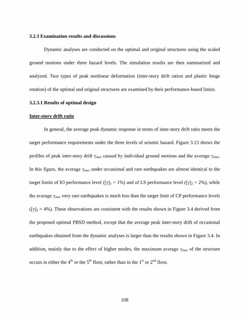
108

3.2.3 Examination results and discussions

Dynamic analyses are conducted on the optimal and original structures using the scaled

ground motions under three hazard levels. The simulation results are then summarized and

analyzed. Two types of peak nonlinear deformation (inter-story drift ration and plastic hinge

rotation) of the optimal and original structures are examined by their performance-based limits.

3.2.3.1 Results of optimal design

Inter-story drift ratio

In general, the average peak dynamic response in terms of inter-story drift ratio meets the

target performance requirements under the three levels of seismic hazard. Figure 3.13 shows the

profiles of peak inter-story drift γmax caused by individual ground motions and the average γmax.

In this figure, the average γmax under occasional and rare earthquakes are almost identical to the

target limits of IO performance level ([γ]1 = 1%) and of LS performance level ([γ]2 = 2%), while

the average γmax very rare earthquakes is much less than the target limit of CP performance levels

([γ]3 = 4%). These observations are consistent with the results shown in Figure 3.4 derived from

the proposed optimal PBSD method, except that the average peak inter-story drift of occasional

earthquakes obtained from the dynamic analyses is larger than the results shown in Figure 3.4. In

addition, mainly due to the effect of higher modes, the maximum average γmax of the structure

occurs in either the 4th

or the 5th

floor, rather than in the 1st or 2

nd floor.

109

Figure 3.13 Peak inter-story drift ratio for optimal design subjected to ground motions scaled for

(a) occasional earthquakes; (b) rare earthquakes; and (c) very rare earthquakes

0

1

2

3

4

5

6

7

0.0% 0.2% 0.4% 0.6% 0.8% 1.0% 1.2% 1.4%

Sto

ry N

um

ber

Inter-story Drift Ratio

Individual recorderMeanMean +/- S.D.Limit = 1%

0

1

2

3

4

5

6

7

0.0% 0.5% 1.0% 1.5% 2.0% 2.5% 3.0%

Sto

ry N

um

ber



0

1

2

3

4

5

6

7

0.0% 1.0% 2.0% 3.0% 4.0% 5.0%

Sto

ry N

um

ber



(c)

(b)

(a)

110

Table 3.7 shows that, for all three hazard levels, the maximum standard deviations (S.D.)

of the peak inter-story drift appear on the 3rd

story, above which the section sizes of beams and

columns change. The relative variability of the inter-story drift is measured by the coefficient of

variation (COV), the ratio between S.D. and the mean value. Because the values of COV are

similar among the three hazard levels, a similar dispersion exists even though the nonlinearity of

the structure as well as hazard levels are different.

Table 3.7 Maximum standard deviation of inter-story drift ratios of optimal structure

2%/50 year 10%/50 year 50%/50 year

Story of max. S.D. 3 3 3

Maximum S.D. 0.0077 0.0044 0.0020

Mean drift ratio of max. S.D. 0.0272 0.0161 0.0076

COV 0.28 0.27 0.26

Plastic hinge rotation

The rotation capacity of a plastic hinge varies during dynamic loading due to the change

in beam shear or column axial force. Thus, a normalized plastic hinge rotation, defined as the

ratio of average peak plastic hinge rotation demand to capacity (θmax/[θ]p), is considered (p = 1, 2,

3 for IO, LS and CP performance levels, respectively). Figure 3.14 shows the location of

normalized plastic hinge rotation for the three levels of seismic hazard. Under occasional

earthquakes, only one ground excitation causes yielding and, as shown in Figure 3.14(a), the

yielding occurs only in a few beams on the 4th

and 5th

stories. Under rare earthquakes, all the

beams yield (Figure 3.14(b)). The normalized plastic hinge rotation ranges from 0.20 to 0.518 and

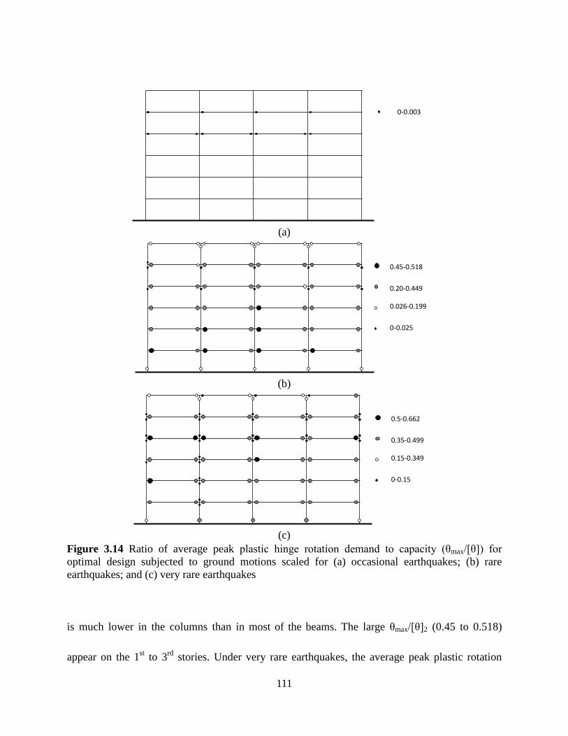
111

is much lower in the columns than in most of the beams. The large θmax/[θ]2 (0.45 to 0.518)

appear on the 1st to 3

rd stories. Under very rare earthquakes, the average peak plastic rotation

(a)

(b)

(c)


optimal design subjected to ground motions scaled for (a) occasional earthquakes; (b) rare

earthquakes; and (c) very rare earthquakes

0-0.003

0.45-0.518

0.026-0.199

0.20-0.449

0-0.025

0.5-0.662

0.15-0.349

0.35-0.499

0-0.15

112

demand is less than 67% of capacity in any member (Figure 3.14(c)). The large θmax/[θ]3 (0.5 to

0.662) appear on the 3rd

to 4th

stories. Figure 3.14(c) also shows that the normalized column

plastic rotations at the supports of the exterior columns are less than that of the three interior

columns.

As shown in Figures 3.14(b) and 3.14(c), column yielding occurs at the upper stories,

which is not predicted by the nonlinear static analyses, indicating the effects of higher vibration

modes. Note that even though the average peak plastic hinges appear at both ends of all the

columns on the same story, these plastic hinges occur at different time or under different

earthquake recorders; thus weak story failure mechanism does not appear.

3.2.3.2 Result of original design

Inter-story drift ratio

In general, the force-based design is conservative, because the average peak inter-story

drifts are far less than the target performance requirements under the three hazard levels, as

shown in Figure 3.15, the values of the maximum γmax/[γ] among all stories are 0.73, 0.81 and

0.59 for the occasional, rare and very rare earthquakes, respectively. This observations is

consistent with the optimal results derived from the optimal PBSD, in which the largest and

smallest γmax/[γ] appear under rare and very rare earthquakes, respectively. In addition, the effect

of higher modes occurs on the model, because the maximum average γmax appears on the 5th

floor.

113

Figure 3.15 Inter-story drift ratio for original design subjected to ground motions scaled for (a)

occasional earthquakes; (b) rare earthquakes; and (c) very rare earthquakes

0

1

2

3

4

5

6

7

0.0% 0.2% 0.4% 0.6% 0.8% 1.0% 1.2%

Sto

ry N

um

ber



0

1

2

3

4

5

6

7

0.0% 0.5% 1.0% 1.5% 2.0% 2.5%

Sto

ry N

um

ber



0

1

2

3

4

5

6

7

0.0% 0.5% 1.0% 1.5% 2.0% 2.5% 3.0% 3.5% 4.0% 4.5%

Sto

ry N

um

ber



(c)

(b)

(a)

114

Table 3.8 shows that, for all three hazard levels, the maximum S.D. of the peak

inter-story drift appears on the 5th

story, where the maximum peak inter-story drift occurs. The

values of COV for both optimal and original structures are similar, which indicates that an

identical dispersion exist even though the strength and stiffness of the structures as well as

hazard levels are different.

Table 3.8 Maximum standard deviation of inter-story drift ratio of original structure

2% / 50 year 10% / 50 year 50% / 50 year

Story of max. S.D. 5 5 5

Maximum S.D. 0.0073 0.004 0.0018

Mean drift ratio of max. S.D. 0.0239 0.0163 0.0073

COV 0.31 0.25 0.25

Plastic hinge rotation

No plastic hinge appears on the original structure under the ground motions scaled for

occasional earthquakes. Figure 3.16 shows the distribution of normalized plastic hinge rotation

for two greater levels of seismic hazard. The maximum normalized plastic hinge rotations are

0.43 and 0.47 for the rare and very rare earthquakes, respectively. Under rare earthquakes, all the

beams and some columns on the 5th and 6th stories yield (Figure 3.16(a)). As shown in this

figure, most large values of θmax/[θ]2 (0.2 to 0.425) appear on the 3rd

to 5th

stories. Under very

rare earthquakes, large values of θmax/[θ]3 (0.35 to 0.472) appear on the 3rd

to 5th

stories (Figure

3.16(b)). Column yielding occurs in the upper stories, which is not predicted by the nonlinear

static analyses, indicating the effects of higher vibration modes.

115

(a)

(b)


original structure subjected to ground motions scaled for (a) rare earthquakes and (b) very rare

earthquakes

3.3 Verification of the Optimal Design

To verify whether the feasible region boundary has an abrupt change around the optimal

design, further analyses are extended to the seismic response and construction cost of the eight

structures with the design variable values close to the optimal design (λ = 0.55, α = 0.70).

Compared with the nonlinear static analysis used in the proposed optimal PBSD method,

nonlinear dynamic analysis can better reflect the actual structural response under the seismic

effect. Therefore, the dynamic analyses are performed on the eight structures to obtain their

0.026-0.199

0.20-0.425

0-0.025

0.15-0.349

0.35-0.472

0-0.15

116

seismic response. The values of pairs of λ and α used to design these eight structures are (0.5,

0.65), (0.5, 0.7), (0.5, 0.75), (0.55, 0.65), (0.55, 0.75), (0.6, 0.65), (0.6, 0.7), and (0.6, 0.75) as

shown in Figure 3.17(a). Based on the method described in Section 2.2.3.3, these nine points are

(a)

(b)

Figure 3.17 Feasible region and the design variables of nine structures in (a) λ–α domain and (b)

Ωc–Ws domain

0.2

0.3

0.4

0.5

0.6

0.7

0.8

0.9

1

1.1

0.1 0.2 0.3 0.4 0.5 0.6 0.7 0.8 0.9 1 1.1

Rela

tive

Str

en

gth

Fa

cto

r α


Nine points for validation

Maximum reinforcement ratio







Optimal design

(α = 0.7, λ = 0.55)

15

16

17

18

19

20

220 240 260 280 300 320

To

tal W

eig

ht o

f L

on

gitu

din

al R

ein

forc

em

en

t W

s

(to

n)


Original design

Nine points for validation


Objective function (considering

both material and labor costs)a

b

c

d

e

f

g

h

i

Optimal design

(α = 0.7, λ = 0.55)

117

transformed from the λ–α domain to the Ωc–Ws domain shown in Figure 3.17 (b) to show the

corresponding material consumptions.

The eight structures are designed based on the values of corresponding λ and α shown in

Figure 3.17 (a) and requirements of ASCE 7-10 (2010). Nonlinear analysis models of these eight

structures are established based on the method given in Section 3.1.2. Dynamic analyses are

performed on the eight structures to obtain the peak normalized deformations. Ten earthquake

records selected in Section 3.2.2.1 are adopted to simulate the seismic effect. These records are

scaled based on the response spectra of the three hazard levels, very rare, rare, and occasional

earthquake hazard levels, as mentioned in Section 3.2.2.2. The peak normalized deformations,

γmax/[γ] and θmax/[θ], of the structures under a hazard level are the average values of the

normalized deformations caused by the ten ground motions.

The dynamic analysis results for each of the eight structures indicate that the peak

inter-story drift ratio of the structure under rare earthquake governs the peak normalized

deformations. This observation is consistent with the peak normalized deformation of the

optimal design (λ = 0.55, α = 0.70). Figure 3.18 shows the values of peak normalized inter-story

drift ratio of the eight structures and the structure with optimal design under rare earthquake. In

this figure, the peak inter-story drift ratio of seven structures, including the optimal design, is

larger than 1.0, that is, the nonlinear deformations of these structures exceed performance limits.

For the other two structures (λ = 0.6, α = 0.7 and λ = 0.6, α = 0.75), the peak normalized

inter-story drift ratio is less than 1.0. Among the eight points and the optimal design, if the values

118

of λ are identical, the value of γmax/[γ] increase with the decline of α, except point d; if the values

of α are identical, the value of γmax/[γ] increase with the reduction of λ, except point g. The value

of γmax/[γ] at points d and g are very close to that of the points around them. Therefore, in general,

a continuous variation tendency exists in the area determined by the eight points without abrupt

change. In addition, the optimal solution determined from dynamic analyses must be located

within the area determined by points b, c, e, f, h, and i.

Figure 3.18 Peak inter-story drift ratio of the nine structures under rare earthquake derived from

dynamic analyses and the feasible region boundary determined from static analyses.

To further illustrate the continuous tendency in the area determined by eight points,

contours of γmax/[γ] are generated form linear interpolation and shown in Figure 3.19, based on

the values of γmax/[γ] for the structures design with the nine pairs of α and λ shown in Figure 3.18.

The second contour line (in red color) from the right represents γmax = [γ]. The optimal solution

0.6

0.62

0.64

0.66

0.68

0.7

0.72

0.74

0.76

0.78

0.8

0.45 0.5 0.55 0.6 0.65

Rela

tive

Str

en

gth

Fa

cto

r α




γmax/[γ] = 1.098 γmax/[γ] = 1.035 γmax/[γ] = 0.989



a b c

d e f

g h i

Structures with γmax > [γ]

Structures with γmax ≤ [γ]

119

determined from dynamic analyses must be located on this contour line. The tendency of all the

contours in Figure 3.19 is continuous especially for the area determined by points b, c, e, f, h,

and i.

Figure 3.19 Contours of the peak normalized inter-story drift ratio and the design variables of

the nine structures

Figure 3.20 shows the total construction cost including the cost of both concrete and

reinforcement of nine structures. For the structures with identical λ value, the concrete

consumptions are identical, and the reinforcement consumptions increase with the value of α.

Due to the increase in section dimension, the required reinforcement area generate identical

element flexural strength is reduced. Thus, the reinforcement consumption of the structures with

identical α value decreases with the rise of λ. In Figure, 3.20, the construction cost of the optimal

design derived from the proposed method is 3% less than the maximum construction cost among

0.9

9

1

1

1.0

1

1.0

1

1.0

2

1.02

1.0

3

1.03

1.0

4

1.04

1.0

5

1.05

1.0

6

1.06

1.0

7

1.07

1.0

8

1.08

1.0

9

1.09

1.09

1.1

1.1

0.5 0.51 0.52 0.53 0.54 0.55 0.56 0.57 0.58 0.59 0.60.65

0.66

0.67

0.68

0.69

0.7

0.71

0.72

0.73

0.74

0.75

Relative stiffness factor λ

Re

lative

str

en

gth

fa

cto

r α

Optimal Design

γmax/[γ] = 1.046

1

1

Structures with γmax > [γ]Structures with γmax ≤ [γ]

a cb

d fe

g ih

120

the eight points at point c. However, the construction cost of the optimal design is about 20% less

than the initial design derived from the force-based seismic design method.

Figure 3.20 Construction cost of the nine structures for verifying the validity of the proposed

optimal PBSD method.

16.5

17

17.5

18

18.5

19

220 225 230 235 240 245 250

To

tal W

eig

ht o

f L

on

gitu

din

al R

ein

forc

em

en

t W

s

(to

n)



Objective function (considering

both material and labor costs)

a

b

c

d

e

f

g

h

i

$108,778

$107,753

$108,265

$111,722

$110,737

$111,229

$114,632

$113,691

$114,156

Structures with γmax > [γ]

Structures with γmax ≤ [γ]

121

CHAPTER 4

RELIABILITY EVALUATION OF PROTOTYPE BUILDING

4.1 Overview of Reliability Evaluation

The prototype structure designed by the conventional force-based seismic design method

is conservative. The degree of conservatism is reduced when the prototype structure is optimized

by the optimal PBSD method. For the optimal structure, one or more types of deformation are

equal to their performance limits. The deformations of this optimal structure and the limits are

derived based on the nominal values of external loads, model parameters, and deformation limits.

However, large uncertainties exist in these three aspects; thus, the deformations of the optimal

structure may be larger than their limits in some extreme conditions. For economic reasons, these

extreme conditions are not eliminated. However, the probability of occurrence of these extreme

conditions shall be controlled to make sure that the optimal design has sufficient reliability.

Accordingly, the reliability evaluation is necessary for the optimal design derived from the

proposed optimal PBSD method. Reliability evaluation is also applied to the original design to

compare with the evaluation results of the optimal design. Furthermore, reliability evaluations

are performed on the other 26 structures with different relative strength factor α and relative

stiffness factor λ to observe how these two variables affect the probability of occurrence of the

extreme conditions.

The reliability evaluations include three procedures in this study. First, Latin Hypercube

122

sampling method is used to select the discrete values of the random variables, and combines

these discrete model parameters to create 8000 structure model samples for both the optimal and

the original structures. Second, 8000 samples are simulated by nonlinear dynamic analysis

method for the peak normalized deformation (θ/[θ] and γ/[γ]). Third, the outputs of these samples

are used to generate the regression lines of peak normalized deformation and fragility function

curves. In addition, to analyze how relative strength factor α and relative stiffness factor γ affect

the reliability evaluation results, the previous procedures are applied on 28 structures besides the

optimal and original structures with seven α levels (α = 0.4, 0.5, 0.6, 0.7, 0.8, 0.9, and 1.0) and

four λ levels (λ = 0.55, 0.7, 0.85, 1.0). The structure nonperformance contours are generated

based on the results of these structures.

4.2 Statistical Properties of Variables

Uncertainty exists in diverse aspects of structural seismic response, and can be derived

from five sources (Bulleit, 2008): time (future external loads and structural characteristics

affected by time), statistical limits (lack of data for their probabilistic distribution), model

limitation (simplifications and assumptions within models), randomness (uncertainty in structural

properties), and human error (mistakes in design and construction). These uncertainties can be

classified into three types (Ayyub and McCuen, 2016): stochastic, epistemic and numerical

uncertainty. Stochastic uncertainty reflects the unpredictability of natural hazard, such as seismic

and snow loads; thus, this type of uncertainty is unavoidable. Epistemic uncertainty is caused by

123

the lack of statistical data or knowledge of understanding. Numerical uncertainty exists when a

mechanical model is adopted to simulate actual buildings, such as when the finite-element

method is used.

Large uncertainties exist in the external loading, structure model for simulation and

performance limits. In this study, the uncertainties in seven aspects (dead load, live load, seismic

effect, flexural strength and effective stiffness of elements, and the limits of inter-story drift and

plastic hinge rotation) are considered. In addition, the uncertainty in some other aspects, such as

structural damping ratio, site condition type, and deterioration of strength and stiffness of plastic

hinge model, also influence the structural nonlinear deformation. However, they are not

considered in this study due to the lack of statistical data. The statistical properties of seven types

of uncertainties are shown in Table 4.1. In this table, x and xn are the mean value and the

nominal value of parameter x; λ is the bias factor, which is the ratio between the mean value and

the nominal value of one type of parameter x; Vs is the coefficient of variation, which is the ratio

between the standard deviation (σx) and mean value of parameter x. Vs is a standardized measure

of dispersion of a probability distribution.

124

Table 4.1 Summary of statistical properties of input variables

Random Variable Type Mean

( x )

Bias Factor

( λn

x

x )

Coefficient of

Variation

(σx

xVx

)

Type of Distribution

Dead load (DL) ‒ 1.05 0.10 Normal

(Ellingwood 1980)

Live load (LL) ‒ 1.00 0.25 Type Ⅰ (Gumbel)

(Ellingwood 1980)

Flexural Strength (M)

(Reinforced Concrete,

Grade 60)

‒ 1.1025 0.11 Normal

(Ellingwood 1980)

Inter-story

drift limit ([γ]) ‒ 1.00 0.1

Lognormal

(SEAOC 1995)

Plastic hinge

rotation limit ([θ]) ‒ 1.00 0.1

Beta

(SEAOC 1995)

Seismic effect

(PGA) 0.1156 ‒ 5.48

Lognormal

(Abrahamson et al.

2014)

Ratio between effective

stiffness and gross

stiffness (EIeff / EIg)

0.403 ‒ 0.643

Lognormal

(Elwood et al. 2007)

Fitting based on Matlab

4.2.1 Statistical properties of external loads

External loading can be divided into two groups. The first group includes dead load (DL)

and live load (LL) applied vertically as constant loading in this study. The second group includes

seismic load (E) applied horizontally as period loading. The uncertainties of DL and LL are

simulated by applying random value generated based on their statistical properties on different

beams and joints. On the other hand, the uncertainty of earthquake exists in peak ground

acceleration (PGA), duration, and frequent content of earthquakes. Many studies(Abrahamson et

al., 2014; Boore et al., 2014; Campbell and Bozorgnia, 2014; Chiou and Youngs, 2014; and Idriss,

125

2014) focused on the statistical properties of PGA, but none for duration or frequent content.

Therefore, the uncertainty of PGA is simulated by the statistical parameters listed in Table 4.1,

and the uncertainty of duration and frequency content is simulated by 10 earthquake recorders

listed in Table 3.5.

4.2.1.1 Dead load and live load

As suggested by Ellingwood (1980), probability distribution types of DL and LL are

assumed to be normal and Type Ⅰ (Gumbel), respectively. Classic probability density function

(PDF) curves for these two types of distribution are shown in Figure 4.1. These probability

distribution types are widely used in many studies (Gaxiola et al., 2017; Kogut and Chou, 2004;

and Ellingwood, 2003). The corresponding bias factor and coefficient of variation listed in Table

4.1 are based on a 50-years reference period. For the nominal live load, Ln, Ellingwood (1980)

suggested that it can be calculated by Equation 4.1 based on A58 standard (1980). The nominal

value calculated by this equation is statistical equal to the 50-year mean value, L. Therefore the

bias factor λ(the ratio between the mean value to the nominal value) for live load is assumed as

1 in this study.

0

150 25n

I

L . LA

Equation 4.1

where AI is influence area and L0 is basic unreduced live load based on A58 (1980).

126

(a)

(b)

Figure 4.1 Probability density function (PDF) curve of: (a) normal distribution; and (b) Type Ⅰ

distribution

The nominal value of DL includes the self-weight of all components (beams, columns

and slabs), and superimposed dead load (roofing, curtain wall, and mechanical). The nominal

value of LL includes the weight of building users, furniture and other moveable equipment.

4.2.1.2 Seismic load

The seismic load applied on a RC moment frame structure is influenced mainly by the

intensity measurement, duration, and frequency content of an earthquake. Many factors can

0

0.05

0.1

0.15

0.2

0.25

0.3

0.35

0.4

0.45

-3 -1 1 3 5

μ = 1

σ = 1

2

2

22

μ1μ σ

2σ2πσ

xf x | , exp

0

0.05

0.1

0.15

0.2

0.25

0.3

0.35

0.4

-2 0 2 4 6 8

μ = 1

β = 1

1 μ μ

μ ββ β β

x xf x | , exp exp

127

describe the intensity measurement of earthquake, such as peak ground acceleration (PGA) or

peak ground velocity. PGA is the most widely used, and conveniently applied in the dynamic

structural analysis. The statistical properties of PGA at a specific location can be determined

through different types of attenuation formulations, which correlate ground motion magnitude to

the distance away from fault rupture. These formulations were established in 2008 and updated

in 2014 by five separate research teams: Abrahamson et al. (2014), Boore et al. (2014), Campbell

and Bozorgnia (2014), Chiou and Youngs (2014), and Idriss (2014). In this study, the statistical

properties of PGA are determined by the next-generation attenuation proposed by Abrahamsonet

al. (2014), and listed in Table 4.1. This attenuation formulation was established based on 2754

ground motion records from 135 earthquakes, and considered the effect of fault type and

geometry, hanging wall effect, site type and other factors. The probability distribution type of

PGA is normally assumed as lognormal (Yazdani et al., 2016; Khatibinia et al., 2013; and Huyse

et al., 2010). Classic PDF curve of lognormal distribution is shown in Figure 4.2.

Figure 4.2 Probability density function curve of lognormal distribution

0

0.2

0.4

0.6

0.8

1

1.2

0 1 2 3 4 5

μ = 1

σ = 1

2

2

2

ln μ1 1μ σ

2σσ 2π

xf x | , exp

x

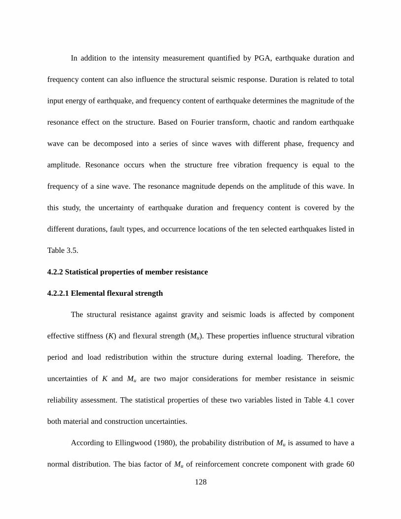
128

In addition to the intensity measurement quantified by PGA, earthquake duration and

frequency content can also influence the structural seismic response. Duration is related to total

input energy of earthquake, and frequency content of earthquake determines the magnitude of the

resonance effect on the structure. Based on Fourier transform, chaotic and random earthquake

wave can be decomposed into a series of since waves with different phase, frequency and

amplitude. Resonance occurs when the structure free vibration frequency is equal to the

frequency of a sine wave. The resonance magnitude depends on the amplitude of this wave. In

this study, the uncertainty of earthquake duration and frequency content is covered by the

different durations, fault types, and occurrence locations of the ten selected earthquakes listed in

Table 3.5.

4.2.2 Statistical properties of member resistance

4.2.2.1 Elemental flexural strength

The structural resistance against gravity and seismic loads is affected by component

effective stiffness (K) and flexural strength (Mu). These properties influence structural vibration

period and load redistribution within the structure during external loading. Therefore, the

uncertainties of K and Mu are two major considerations for member resistance in seismic

reliability assessment. The statistical properties of these two variables listed in Table 4.1 cover

both material and construction uncertainties.

According to Ellingwood (1980), the probability distribution of Mu is assumed to have a

normal distribution. The bias factor of Mu of reinforcement concrete component with grade 60

129

reinforcement was assumed to be 1.05 based on static loading experiments. However, the

strength of concrete and reinforcement tends to increase by 5% due to a high loading rate under

earthquakes. Therefore, in the dynamic analysis, the bias factor of Mu is also increased by 5% so

that it is equal to 1.1025. The nominal value of Mu is determined by the seismic design of RC

moment frame structure.

4.2.2.2 Elemental effective stiffness

Due to concrete cracking and bar slip, the K of a RC component under seismic loads is

less than that evaluated based on gross section. In addition, shear deformation is found to occupy

15% of total component deformation (Elwood and Eberhard, 2009; and Kenneth et al. 2009).

Therefore, total effective displacement of RC component should include the deformations caused

by flexure, longitudinal bar bond slip, and shear deformation. K is the reciprocal of total effective

displacement under unit load.

No study has ever suggest the distribution type, mean value or standard deviation of K.

Nevertheless, Elwood and Eberhard (2006) collected 221 experiment results of the ratio between

the effective flexural stiffness, EIeff, and the gross bending stiffness, EIg, of rectangular column,

as shown in Figure 4.3.

130

Figure 4.3 Measured ratio between effective stiffness and gross bending stiffness (Elwood et al.,

2007)

Although only the flexural experiments of column are summarized in these results, beam can be

taken as a flexural component without axial load. Therefore, in this study, the K of beams and

columns are assumed to have statistical properties identical to those of the experimental data

given by Elwood and Eberhard (2009). However, in these papers, neither the distribution type or

the statistical properties of the ratio between effective stiffness and gross stiffness is not given.

Therefore, Matlab distribution fitting toolbox is used in this study to obtain a suitable probability

distribution type and corresponding statistical properties of K. First, 221 discrete value of the

ratio between effective stiffness and gross stiffness are distributed into twelve frequency

histogram columns with an interval of 0.1 stiffness ratio, as shown in Figure 4.4(a). Then,

eighteen distribution types in Matlab toolbox are used to fit this frequency histogram of stiffness

data without excluding the extreme value. Based on the fitting results, Lognormal and

131

Birnbaum-Saunders distributions are suitable to the discrete data of the stiffness ratio with log

likelihood factor 41.51 and 43.89. A higher log likelihood factor expresses a better fitting

between the PDF or CDF curve and the frequency distribution histogram. At last, Lognormal

distribution is chosen as the probability distribution type of the stiffness ratio in this study,

because it is more widely used than Birnbaum-Saunders distribution. The corresponding

(a)

(b)

Figure 4.4 Distribution fitting of discrete stiffness ratio (a) frequency histogram of discrete

stiffness ratio and PDF of fitting lognormal distribution; (b) cumulate frequency histogram of

stiffness ratio and CDF of fitting lognormal distribution

132

mean value and COV are listed in Table 4.1. The cumulative distribution function curve can

closely match the discrete data, as shown in Figure 4.4(b).

In Figure 4.4(a), 221 discrete experiment data in Elwood and Eberhard (2009) are

distributed into twelve frequency histogram columns. Eighteen distribution types in Matlab

toolbox are used to fit this frequency histogram of stiffness data without excluding the extreme

value. Based on the fitting results, Lognormal and Birnbaum-Saunders distributions are suitable

to the discrete data of the stiffness ratio with log likelihood factor 41.51 and 43.89. A higher log

likelihood factor expresses a better fitting between the PDF or CDF curve and the frequency

distribution histogram. As the most widely used distribution type, Lognormal distribution is

chosen as the probability distribution type of the stiffness ratio in this study. The corresponding

mean value and COV are listed in Table 4.1. The cumulative distribution function curve can

closely match the discrete data, as shown in Figure 4.4(b).

4.2.3 Statistical properties of deformation limits

Inter-story drift and plastic hinge rotation are two major deformation measurements of

the seismic performance assessment of RC moment frame structure. However, no sufficient

information is provided in ASCE 41-13 (2014), the standard used in this study for

performance-based seismic evaluation, to select appropriate bias factor or COV for allowable

values of inter-story drift [γ] and plastic hinge rotation [θ]. In addition to ASCE 41-13 (2014),

SEAOC (1995) can be used to assess seismic performance. In this document, the statistical

properties of inter-story drift, local damage index and global damage index are provided. The

133

local damage index, considering both component section rotation and energy dissipation effect,

is defined by Park and Ang (1985) and Moller et al. (2009), as

d0 25

m y

u y y u

ELDI .

M

Equation 4.2

where ϕm is the maximum cross-sectional rotation; ϕu is the ultimate rotation during a monotonic

load; ϕy is the recoverable rotation during unloading; dE is the energy dissipation caused by

hysteretic deformation; and My is section yield moment. In Equation 4.2, both section rotation

part and energy dissipation part are impact mainly by plastic hinge rotation; thus, it is rational to

assume [θ] and local damage index have identical statistical properties. In this study, [θ] is

assumed to have Beta distribution, which is the distribution type of local damage index in

SEAOC (1995). A classic Beta distribution is drawn in Figure 4.5. The value of [γ] and [θ] in

ASCE41-13 are used as the nominal value, and the bias factor is assumed to be 1.0.

Figure 4.5 Probability density function curve of Beta distribution

0

0.2

0.4

0.6

0.8

1

1.2

1.4

1.6

0 0.2 0.4 0.6 0.8 1

α = 2

β = 2

β 1α 1 1α β

B α β

x xf x | ,

,

α βB α β

α β,

134

4.3 Sampling Methods

Sampling method is a survey methodology used to predict statistical properties of whole

sample population by repeatedly testing a finite number of samples within this population. For

this purpose, simulations by performing nonlinear dynamic structural analyses of the optimized

structure with seven input parameters are conducted in this study.

4.3.1 Monte Carlo sampling method

Monte Carlo sampling method is a conventional sampling method, which has been used

so solve statistical problems in many fields. Monte Carlo sampling method repeats random

sampling of input variables and experimental or numerical simulation to obtain a probabilistic

distribution of the results. Monte Carlo sampling method is reliable; however, the difficulty of

using this method in practice is its extremely high experimental or computational cost for

complex system or small probability of occurrence. In a structural seismic failure simulation,

complex nonlinear dynamic analysis is applied to obtain the nonlinear deformation of the

structure considering the uncertainties within seismic records. In addition, the allowable failure

probability of the structure under the very rare earthquake is as small as 0.001 (Paulay and

Priestley, 1992). Therefore, the required sampling number is enormous and even impracticable.

Soong and Grigoriu (1993) proposed a method to estimate the approximate number required for

using Monte Carlo sampling method, as shown in Equation 4.3.

135

3

2 2 3

1 1 10399600

0 05 10

PN

V P .

Equation 4.3

where N is the required number of samples; P is the estimated failure probability; and V is the

COV of sample population. Based on Equation 4.3, the required sampling number of Monte

Carlo sampling method for the problem with a 0.001 failure probability and 5% COV is 399600.

Although controversy exists about the exact required number of samples in the Monte Carlo

sampling method (Shooman, 1968; Soong and Grigoriu 1993), it is definitely an extreme large

number, and difficult to be applied to the failure probability analysis of RC frames.

4.3.2 Latin Hypercube sampling method

An alternative approach is Latin Hypercube sampling method proposed by Iman and

Conover (1980). It is a near-random sampling method to estimate the probability properties of

the sample population. The Latin Hypercube sampling method requires smaller sampling number

than Monte Carlo sampling method, and has been proved to be effective and reliable in

evaluating the structural failure probabilities under seismic or wind load effect (Yazdani et al.,

2016; Li and Hu, 2014; and Khatibinia et al., 2013).

4.3.2.1 Procedure of Latin Hypercube sampling method

To select near-random input variables for each sample by Latin Hypercube sampling

method, two steps are used to establish a N×K input variable matrix with a total sample number

of N and a total number of input variable types of K shown in Figure 4.6(d). First, for every type

of input variable, such as dead load, N discrete representative values are selected according to the

136

cumulative distribution function of this variable, as shown in Figure 4.6(a). Second, the

sequential order of the selected value of each variable is adjusted according to the table of

random permutation of rank number, as shown in Figure 4.6(c). This procedure is repeated for

every input variable, and the N×K input variable matrix shown in Figure 4.6(d) is established.

The values of the input variables of the ith

sample are the data on the ith

row in the N×K input

variable matrix, and all the discrete representative values of the jth

input variable are the data on

the jth

column in this matrix.

Figure 4.6 Procedure of Latin Hypercube sampling method: (a) representative values selection

from CDF of one variable; (b) frequency histogram and PDF of selected representative values;

(c) order rearranging of representative values of one variable; and (d) input data matrix of all

variables and samples

iN-2i1 i2 i3 iN-1 iN

CDF PDF

…...

…...iN-1 i5 i7 i3 iN-4 iN-10

small ‒ large

random

…...

iN-1

i5

i7

i3

iN-4

iN-10

…...

1N-9

12

16

17

1N

1N-8

…...

N13

N9

NN-2

N5

NN-4

NN-1

…...

…...

…...

…...

Variable type (K)

Sam

ple

Num

. (N

)

i1 i2 i3 iNiN-1iN-2

Sample j

Equal

interval

(a) (b)

(c) (d)

Table of random permutation

of rank number

Variable i

1.0

137

To obtain N discrete representative values of a variable in the first step, cumulative

distribution function curve of this variable is separated into N intervals with identical difference

in probability, as shown in Figure 4.6(a). The frequency histograms of these selected values

shown in Figure 4.6(b) still statistically obey the probability density function of this variable

shown in Figure 4.6(a). The representative value of each interval is the variable value with a

centroid probability of the corresponding interval defined in Equation 4.4. Currently, all selected

values are ordered from small to large. In the second step, the small-to-large ordered

representative values are rearranged according to the table of random permutation of rank

number into a random order, as shown in Figure 4.6(c). The rank number of this variable is an

arrange of integers [1, 2, ... N]T coupling to the selected representative values in a small-to-large

order. In the table of random permutation of rank number, this rank number is rearranged

randomly to reflect the uncertainty in nature. These two steps are repeated for K variables, and a

N×K matrix is established, as shown in Figure 4.6(d). The data on the ith

column of this matrix

are the representative values in random order of variable i, and the data on the jth

row are the

input values of variables of sample j. Eventually, the data of this matrix are inputted into N

models for numerical or experimental simulations.

1 0 5nKK

m .F

N

Equation 4.4

where F‒1

K is inverse cumulative distribution function of variable K, and mnK is rank number of

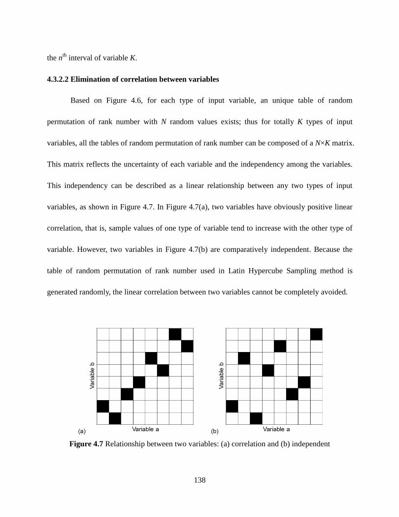
138

the nth

interval of variable K.

4.3.2.2 Elimination of correlation between variables

Based on Figure 4.6, for each type of input variable, an unique table of random

permutation of rank number with N random values exists; thus for totally K types of input

variables, all the tables of random permutation of rank number can be composed of a N×K matrix.

This matrix reflects the uncertainty of each variable and the independency among the variables.

This independency can be described as a linear relationship between any two types of input

variables, as shown in Figure 4.7. In Figure 4.7(a), two variables have obviously positive linear

correlation, that is, sample values of one type of variable tend to increase with the other type of

variable. However, two variables in Figure 4.7(b) are comparatively independent. Because the

table of random permutation of rank number used in Latin Hypercube Sampling method is

generated randomly, the linear correlation between two variables cannot be completely avoided.

Figure 4.7 Relationship between two variables: (a) correlation and (b) independent

139

A modified Latin Hypercube sampling method using specifically modified tables of

random permutations of ranked number and Spearman coefficient is proposed by Yang (2006) to

eliminate this linear correlation. First, a measurement of the correlation level called Spearman

rank-order correlation coefficient (Spearman coefficient) is proposed by Hettmansperger and

McKean (1978) and defined as follows. The N representative values of two variables, P and Q,

are selected and arranged from small to large with same rank numbers [1, 2, ... n]T. To reflect

uncertainty of the nature, the order of Qi is changed according to one table of random

permutation of rank number, that is, the rank number of Qi becomes to [R1, R2, ... Rn]T ≠ [1, 2, ...

n]T, where Ri is corresponding to the out-of-order rank number of Qi. The Spearman coefficient rs

between variables P and Q can be defined by Equation 4.5. Spearman coefficient is always

located between ‒1 and +1, which reflect the negative and positive linear correlations exist

between two variables. Thus the more Spearman coefficient close to zero, the more two variables

get independent.

1

2 2

1 1

1 1

2 2

1 1

2 2

n

i

is

n n

i

i i

n ni R

r

n ni R

Equation 4.5

Second, a critical coefficient or threshold should be determined to check whether the

correlation between two variables is higher than necessary. This is because an absolutely

independent relationship between two variables is hard to get due to the limited sampling number.

140

Such an independent relationship is also unnecessary due to its negligible effect on the statistical

probability. Accordingly, threshold Spearman coefficient r*

s is proposed, and the rank number of

two variables is modified if this threshold is exceeded.

If the Spearman coefficient between two variables is higher than r*

s , the following process

can be performed to reduce the undesired correlation. For a system with K variables and, N

sample numbers, the N×K table of random permutations of ranked number is defined as R, in

which the data in column is the random rank number of one of the K variables. A K×K Spearman

coefficient matrix, T, can be established according to Equation 4.5, and Tij represents the

Spearman coefficient between the ith

and jth

variable. Obviously, T is a symmetrical matrix, and

always assumed as positive. T satisfies Equations 4.6 to 4.8. A lower triangular matrix, S, is used

to establish the modified table of random permutations of ranked number, RB. Cholesky

factorization scheme can be used to solve the problem with lower triangular matrix.

1TS T S Equation 4.6

1S Q Equation 4.7

TT Q Q Equation 4.8

where Q is a lower triangular matrix. A modified table of random permutations of ranked number,

RB, can be obtained by Equation 4.9.

T

BR R S Equation 4.9

141

The procedure described above is repeated until no element in T is larger than r*

s , that is,

matrix T gets close to unit matrix. In the current step, this modified table of random permutations

of ranked number can be used to product uncorrelated representative values of variables. It has

been proved that this modified Latin Hypercube sampling method can significantly reduce the

output variance of probability analysis (Yang, 2006). One example of applying modified Latin

Hypercube sampling method is illustrated in Figure 4.8, through eliminating the correlation

between inter-story drift limit and PGA of input earthquake acceleration.

(a)

(b)

Figure 4.8 Illustration of the relationship between two input variables: (a) correlated relationship

(b) independent relationship

4.4 Probability-based Nonperformance Probability

For each structure with determined relative strength and stiffness factors, 8000 samples

are created based on the discrete variables for seven uncertainties selected and combined by

Latin Hypercube sampling method. The deformation of these 8000 samples are estimated by

142

nonlinear dynamic analysis method described in Section 3.2. The examined output data of the

dynamic analysis are two types of peak normalized deformation in terms of plastic hinge rotation

and inter-story drift: peak θ/[θ] and peak γ/[γ].

To determine the reliability of a structure, the probability of nonperformance of this

structure is evaluated by its limits. Nonperformance due to a certain type of deformation is

defined as the peak normalized value of this type of deformation is larger than 1. In this study,

three types of nonperformance are defined: nonperformance due to plastic hinge (peak θ/[θ] > 1),

nonperformance due to inter-story drift (peak γ/[γ] > 1), and nonperformance due to either plastic

hinge or inter-story drift (either peak θ/[θ] > 1 or peak γ/[γ] > 1). Because the values of both [θ]

and [γ] are different for diverse performance levels (CP, LS, and IO performance levels), each

type of nonperformance can be measured by the limit for different performance levels. To define

a nonperformance of a structure, both nonperformance type and performance level shall be

indicated, such as nonperformance due to inter-story drift for LS performance level. For a

structure, the nonperformance due to a certain type of deformation for a performance level

indicates that this type of deformation of the structure cannot satisfy the deformation limit of this

performance level.

For a structure, the probability of nonperformance due to a certain type of normalized

deformation for a performance level, PfE, is the ratio between the number of the samples with

peak normalized deformation larger than 1 and 8000 samples. This nonperformance probability

is for 50-year duration. Because the nonperformance limit suggested by Paulay and Priestley

143

(1992) listed in Table 1.3 is for 1-year duration, the annual probability of nonperformance due to

a certain type of deformation for a performance level, Pf,a, can be calculated based on by

Equation 4.10.

, 1 exp νf a fEP P Equation 4.10

where ν is the mean occurrence rate of the earthquakes, which is normally assumed as ν = 0.2 for

a Poisson process (Khatibinia et al., 2013; Moller et al., 2015).

4.5 Fragility Curve Generation

Fragility function indicates the relationship between the probability of nonperformance

and a intensity measure of ground motion, which can be quantified as the peak ground

acceleration (PGA) (Baker, 2015). In this study, the fragility functions of the optimal and original

structures are generated by the method suggested by Baker (2015) based on the normalized

deformations of 8000 samples. These samples include 800 PGA levels, and 10 types of

earthquake records for each PGA level. First, the nonperformance probability for each PGA,

which is the ratio between the number of nonperformance samples and 10, is obtained. Then, the

median and standard deviation of the nonperformance probability for all PGA are estimated by

maximum likelihood method. Based on the estimated median, μ , and estimated standard

deviation of ln(PGA), σ, a lognormal cumulative distribution function is typically used to create

the fragility function based on Equation 4.11.

144

μ

σ

ln x /P IM x

Equation 4.11

where Φ() is the standard normal cumulative distribution function. The estimated median and

standard deviation instead of the actual ones are used here, because these parameters are derived

from only the samples, which is part of the population.

4.6 Results and Discussion

4.6.1 Normalized deformation

For the optimal and original structures, the peak normalized deformation (peak θ/[θ] and

peak γ/[γ]) of 8000 samples are obtained by nonlinear dynamic analyses. The larger peak

normalized deformations between peak θ/[θ] and peak γ/[γ] of 8000 samples are drawn in Figure

4.9. The single type of peak normalized deformation (peak θ/[θ] or peak γ/[γ]) of 8000 samples

are drawn in Figures 4.10 and 4.11, respectively. In these figures, regression analyses are

performed to obtain a mean value line of peak normalized deformation (solid line) as a function

of peak ground acceleration. The functions of these lines are defined as y = a1x + b1 for the larger

peak normalized deformation between peak θ/[θ] and peak γ/[γ], y = aθx + bθ for peak θ/[θ], and

y = aγx + bγ for peak γ/[γ]. In addition, the 95% confidence band are drawn as the dash lines in

each figure.

Based on the slope a of the regression line, the probability of different types of

nonperformance can be estimated. If the nonperformance probability when either θ/[θ] > 1 or

145

γ/[γ] > 1 is define as 100%, then the probability when both θ/[θ] > 1 and γ/[γ] > 1 can be

calculated by a2 = (aθ + aγ ‒ a1)/a1. The probability when θ/[θ] > 1 but γ/[γ] < 1 can be calculated

by aθ/a1 ‒ a2; similarly, when γ/[γ] > 1 but θ/[θ] < 1, the probability can be calculated by aγ/a1 ‒ a2.

The results of different types of nonperformance are listed in Table 4.2.

Table 4.2 Composition of different types of nonperformance (unit: %)

Performance

level

Optimal Structure Original Structure

θ/[θ] > 1

but

γ/[γ] <1

θ/[θ] < 1

but

γ/[γ] > 1

θ/[θ] > 1

and

γ/[γ] > 1

θ/[θ] > 1

but

γ/[γ] <1

θ/[θ] < 1

but

γ/[γ] > 1

θ/[θ] > 1

and

γ/[γ] > 1

CP 5.3 27.3 67.3 2.9 37.9 59.2

LS 5.5 27.1 67.4 2.5 38.3 59.2

IO 12.5 17.1 70.4 8.0 27.5 64.5

Based on Table 4.2, the probabilities of different types of nonperformance are similar

between CP and LS performance levels. The probability of both θ/[θ] > 1 and γ/[γ] > 1 is much

higher than the other types of nonperformance, while the probability of θ/[θ] > 1 but γ/[γ] < 1 is

much lower than the other types of nonperformance. It can be concluded that (1) the probability

of simultaneous appearance of both types of nonperformance (θ/[θ] > 1 and γ/[γ] > 1) is higher

than the probability due to other types of deformation; (2) nonperformance due to plastic hinge

hardly appears alone without the nonperformance due to inter-story drift; (3) No matter the type

of deformation, the nonperformance probabilities of optimal and original structures are close.

The width of the 95% confidence band w reflects the uncertainty of the normalized

deformation. The width is normalized by the slope of the regression line as w/a to compare the

146

uncertainty of the sample with different magnitudes. The normalized width of the 95%

confidence band of three types of failure for both optimal and original structures in different

performance levels are listed in Table 4.3. In this table, the higher value reflects higher

uncertainty.

Table 4.3 Normalized width of the 95% confidence band (w/a)

Performance level


peak

θ/[θ]

peak

γ/[γ]

max(peak θ/[θ]

& peak γ/[γ])

peak

θ/[θ]

peak

γ/[γ]

max(peak θ/[θ]

& peak γ/[γ])

CP 0.445 0.236 0.243 0.519 0.217 0.221

LS 0.335 0.164 0.165 0.439 0.161 0.163

IO 0.173 0.096 0.094 0.265 0.099 0.102

Based on Table 4.3, the normalized width of the 95% confidence band for peak θ/[θ] is

much higher than the other two types of deformation. the normalized width of the 95%

confidence band for CP performance level is higher than the other two performance levels. It can

be concluded that (1) the uncertainty of normalized plastic hinge is much higher than the other

two types of deformation; (2) the uncertainty of different peak normalized deformation for CP

performance level is higher than the other two types of performance levels.

147

(a)

(b)

(c)

Figure 4.9 Statistical result of the peak normalized plastic deformations (maximum value of

γ/[γ] and θ/[θ]) of the optimal and original design in various performance levels: (a) collapse

prevention; (b) life safety; and (c) immediate occupancy

y = 0.823x + 0.005

0.0

0.2

0.4

0.6

0.8

1.0

1.2

1.4

1.6

0.0 0.2 0.4 0.6 0.8 1.0

ma

x γ

/[γ] a

nd

θ/[θ

]

PGA (g)

Optimal structure

y = 0.683x + 0.001

0.0

0.2

0.4

0.6

0.8

1.0

1.2

1.4

1.6

0.0 0.2 0.4 0.6 0.8 1.0

ma

x γ

/[γ] a

nd

θ/[θ

]

PGA (g)

Pototype structure

y = 1.623x + 0.010

0.0

0.5

1.0

1.5

2.0

2.5

3.0

3.5

0.0 0.2 0.4 0.6 0.8 1.0

ma

x γ

/[γ] a

nd

θ/[θ

]

PGA (g)

Optimal structure

y = 1.305x + 0.004

0.0

0.5

1.0

1.5

2.0

2.5

3.0

3.5

0.0 0.2 0.4 0.6 0.8 1.0

ma

x γ

/[γ] a

nd

θ/[θ

]

PGA (g)

Pototype structure

y = 3.367x - 0.017

0.0

1.0

2.0

3.0

4.0

5.0

6.0

7.0

8.0

0.0 0.2 0.4 0.6 0.8 1.0

ma

x γ

/[γ] a

nd

θ/[θ

]

PGA (g)

Optimal structure

y = 2.630x - 0.015

0.0

1.0

2.0

3.0

4.0

5.0

6.0

7.0

8.0

0.0 0.2 0.4 0.6 0.8 1.0

ma

x γ

/[γ] a

nd

θ/[θ

]

PGA (g)

Pototype structure

148

(a)

(b)

(c)

Figure 4.10 Statistical result of the peak normalized plastic deformations (peak θ/[θ]) of the

optimal and original design in various performance levels: (a) collapse prevention; (b) life safety;

and (c) immediate occupancy

y = 0.598x - 0.064

0.0

0.2

0.4

0.6

0.8

1.0

1.2

1.4

1.6

0.0 0.2 0.4 0.6 0.8 1.0

θ/[θ

]

PGA (g)

Optimal structure

y = 0.424x - 0.056

0.0

0.2

0.4

0.6

0.8

1.0

1.2

1.4

1.6

0.0 0.2 0.4 0.6 0.8 1.0

θ/[θ

]

PGA (g)

Pototype structure

y = 1.183x - 0.126

0.0

0.5

1.0

1.5

2.0

2.5

3.0

3.5

0.0 0.2 0.4 0.6 0.8 1.0

θ/[θ

]

PGA (g)

Optimal structure

y = 0.805x - 0.107

0.0

0.5

1.0

1.5

2.0

2.5

3.0

3.5

0.0 0.2 0.4 0.6 0.8 1.0

θ/[θ

]

PGA (g)

Pototype structure

y = 2.791x - 0.300

0.0

1.0

2.0

3.0

4.0

5.0

6.0

7.0

8.0

0.0 0.2 0.4 0.6 0.8 1.0

θ/[θ

]

PGA (g)

Optimal structure

y = 1.908x - 0.255

0.0

1.0

2.0

3.0

4.0

5.0

6.0

7.0

8.0

0.0 0.2 0.4 0.6 0.8 1.0

θ/[θ

]

PGA (g)

Pototype structure

149

(a)

(b)

(c)

Figure 4.11 Statistical result of the peak normalized plastic deformations (peak γ/[γ]) of the

optimal and original design in various performance levels: (a) collapse prevention; (b) life safety;

and (c) immediate occupancy

y = 0.779x + 0.011

0.0

0.2

0.4

0.6

0.8

1.0

1.2

1.4

1.6

0.0 0.2 0.4 0.6 0.8 1.0

γ/[γ]

PGA (g)

Optimal structure

y = 0.663x + 0.005

0.0

0.2

0.4

0.6

0.8

1.0

1.2

1.4

1.6

0.0 0.2 0.4 0.6 0.8 1.0

γ/[γ]

PGA (g)

Pototype structure

y = 1.534x + 0.022

0.0

0.5

1.0

1.5

2.0

2.5

3.0

3.5

0.0 0.2 0.4 0.6 0.8 1.0

γ/[γ]

PGA (g)

Optimal structure

y = 1.273x + 0.009

0.0

0.5

1.0

1.5

2.0

2.5

3.0

3.5

0.0 0.2 0.4 0.6 0.8 1.0

γ/[γ]

PGA (g)

Pototype structure

y = 2.945x + 0.042

0.0

1.0

2.0

3.0

4.0

5.0

6.0

7.0

8.0

0.0 0.2 0.4 0.6 0.8 1.0

γ/[γ]

PGA (g)

Optimal structure

y = 2.419x + 0.016

0.0

1.0

2.0

3.0

4.0

5.0

6.0

7.0

8.0

0.0 0.2 0.4 0.6 0.8 1.0

γ/[γ]

PGA (g)

Pototype structure

150

4.6.2 Nonperformance probability

For the optimal and original structure, the probabilities of nonperformance due to plastic

hinge rotation, inter-story drift, and either plastic hinge rotation or inter-story drift for three

performance levels are shown in Table 4.4. In addition, the allowable nonperformance

probabilities of different performance levels [PfE] suggested by Paulay and Priestley (1992) are

also listed in this table.

Table 4.4 Probabilities of nonperformance due to different types deformation of the optimal and

original structures


Performance

level [PfE] θ/[θ] > 1 γ/[γ] > 1

either θ/[θ] >

1 or γ/[γ] > 1 θ/[θ] > 1 γ/[γ] > 1

either θ/[θ] >

1 or γ/[γ] > 1

IO 0.100 0.0635 0.1435 0.1464 0.0395 0.0745 0.0770

LS 0.010 0.0095 0.0160 0.0180 0.0031 0.0064 0.0069

CP 0.001 0.0015 0.0005 0.0015 0.0004 0.0000 0.0004

Based on Table 4.4, for the original structure, the probabilities of nonperformance due to

all three types of deformation for all three performance levels satisfy the probability limits

suggested by Paulay and Priestley (1992). For the optimal structure, the probabilities of

nonperformance due to plastic hinge for all three performance satisfy the probability limits. The

probability of nonperformance due to inter-story drift for CP performance level satisfies the

probability limit, while those for LS and IO performance levels are about 50% higher than the

probability limits. The probabilities of nonperformance due to either plastic hinge or inter-story

drift for all three performance levels are about 50% higher than the probability limits. These

151

results indicate that the optimal structure shall be designed based on higher relative strength

and/or relative stiffness factors to ensure that the probabilities of nonperformance satisfies the

probability limits.

4.6.3 Fragility curve of nonperformance probability

The fragility curves of the optimal and original structures are generated by using the

method described in Section 4.5, and drawn in Figures 4.12 and 4.13, respectively. The estimated

median value and estimated standard deviation used to create the lognormal distributed fragility

curves are achieved based on the normalized deformations of the 8000 samples for each structure.

In Figures 4.12 or 4.13, the fragility curves of three types of nonperformance (due to either

plastic hinge or inter-story drift, only due to plastic hinge, and only due to inter-story drift) are

drawn. The fragility curves of each type of nonperformance include three curves for three

performance levels (CP, LS, and IO).

These fragility curves can be used to determine the faillure probability of a structure

under a selected PGA. In this study, the PGA corresponding to very rare, rare, and occasional

earthquakes are 0.6g, 0.4g and 0.174g. In addition, the fragility curves of different performance

levels can be used to define structure damage states: None, slight, moderate and extensive. As

shown in Figure 4.14, these four types of structure damage states can be defined as: (1) none

damage, when deformation is less than deformation limit of IO performance level; (2) slight

damage, when deformation is more than deformation limit of IO performance level but less than

that of LS performance level; (3) moderate damage, when deformation is more than deformation

152

(a)

(b)

(c)

Figure 4.12 Fragility curves for the optimal design in different nonperformance types: (a) either

θ/[θ] > 1 or γ/[γ] > 1; (b) θ/[θ] > 1; and (c) γ/[γ] > 1

0%

10%

20%

30%

40%

50%

60%

70%

80%

90%

100%

0.0 0.1 0.2 0.3 0.4 0.5 0.6 0.7 0.8 0.9 1.0

Pro

ba

bility o

f n

on

pe

rfo

rma

nce

PGA (g)

CP

LS

IO

CP

LS

IO

θ/[θ] > 1

orγ/[γ] > 1

0%

10%

20%

30%

40%

50%

60%

70%

80%

90%

100%

0.0 0.1 0.2 0.3 0.4 0.5 0.6 0.7 0.8 0.9 1.0

Pro

ba

bility o

f n

on

pe

rfo

rma

nce

PGA (g)

CP

LS

IO

CP

LS

IO

θ/[θ] > 1

0%

10%

20%

30%

40%

50%

60%

70%

80%

90%

100%

0.0 0.1 0.2 0.3 0.4 0.5 0.6 0.7 0.8 0.9 1.0

Pro

ba

bility o

f n

on

pe

rfo

rma

nce

PGA (g)

CP

LS

IO

CP

LS

IO

γ/[γ] > 1

153

(a)

(b)

(c)

Figure 4.13 Fragility curves for the original design in different nonperformance types: (a) either

θ/[θ] > 1 or γ/[γ] > 1; (b) θ/[θ] > 1; and (c) γ/[γ] > 1

0%

10%

20%

30%

40%

50%

60%

70%

80%

90%

100%

0.0 0.1 0.2 0.3 0.4 0.5 0.6 0.7 0.8 0.9 1.0

Pro

ba

bility o

f n

on

pe

rfo

rma

nce

PGA (g)

CP

LS

IO

CP

LS

IO

θ/[θ] > 1

orγ/[γ] > 1

0%

10%

20%

30%

40%

50%

60%

70%

80%

90%

100%

0.0 0.1 0.2 0.3 0.4 0.5 0.6 0.7 0.8 0.9 1.0

Pro

ba

bility o

f n

on

pe

rfo

rma

nce

PGA (g)

CP

LS

IO

CP

LS

IO

θ/[θ] > 1

0%

10%

20%

30%

40%

50%

60%

70%

80%

90%

100%

0.0 0.1 0.2 0.3 0.4 0.5 0.6 0.7 0.8 0.9 1.0

Pro

ba

bility o

f n

on

pe

rfo

rma

nce

PGA (g)

CP

LS

IO

CP

LS

IO

γ/[γ] > 1

154

limit of LS performance level but less than that of CP performance level; extensive damage,

when deformation is more than deformation limit of CP performance level. The probablity of

occurrence each damage state of a structure under a specific PGA is defined as pi (i = 1, 2, 3, or 4

for None, slight, moderate or extensive damage states). Probability of nonperformancee of a

structure for a specific PGA is defined as Pj (j = IO, LS, or CP performance level). Therefore,

based on Figure 4.14, pi can be calculated based on Equation 4.12.

1

1 1, IO

2 or 3, IO or LS, 1 LS or CP

4, CP

i j

j j

j

p P i j

P P i j j

P i j

Equation 4.12

Figure 4.14 Defination of the four types of damage states

The pi for both optimal and original structures under three hazard levels (very rare, rare,

and occational earthquake levels) are calculated and summarized in Table 4.5. Three PGA levels

0.0

0.1

0.2

0.3

0.4

0.5

0.6

0.7

0.8

0.9

1.0

0.0 0.1 0.2 0.3 0.4 0.5 0.6 0.7 0.8 0.9 1.0

Pro

ba

bili

ty o

f e

xce

ed

ance

PGA (g)

CP

LS

IONone

Slight

Moderate

Extensive

p1 = 1 ‒ PIO

p2 = PIO ‒ PLS

p3 = PLS ‒ PCP

p4 = PCP

Pro

bab

ility

of

no

np

erf

orm

an

ce

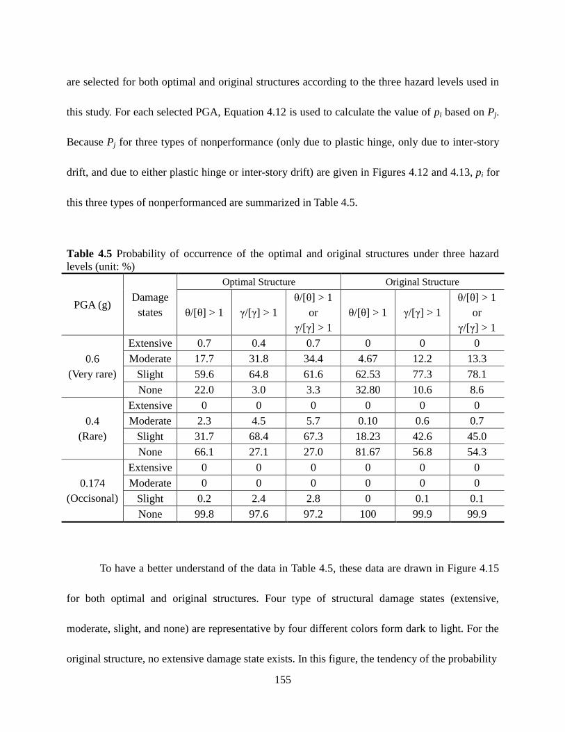
155

are selected for both optimal and original structures according to the three hazard levels used in

this study. For each selected PGA, Equation 4.12 is used to calculate the value of pi based on Pj.

Because Pj for three types of nonperformance (only due to plastic hinge, only due to inter-story

drift, and due to either plastic hinge or inter-story drift) are given in Figures 4.12 and 4.13, pi for

this three types of nonperformanced are summarized in Table 4.5.

Table 4.5 Probability of occurrence of the optimal and original structures under three hazard

levels (unit: %)

PGA (g) Damage

states


θ/[θ] > 1 γ/[γ] > 1

θ/[θ] > 1

or

γ/[γ] > 1

θ/[θ] > 1 γ/[γ] > 1

θ/[θ] > 1

or

γ/[γ] > 1

0.6

(Very rare)

Extensive 0.7 0.4 0.7 0 0 0

Moderate 17.7 31.8 34.4 4.67 12.2 13.3

Slight 59.6 64.8 61.6 62.53 77.3 78.1

None 22.0 3.0 3.3 32.80 10.6 8.6

0.4

(Rare)

Extensive 0 0 0 0 0 0

Moderate 2.3 4.5 5.7 0.10 0.6 0.7

Slight 31.7 68.4 67.3 18.23 42.6 45.0

None 66.1 27.1 27.0 81.67 56.8 54.3

0.174

(Occisonal)

Extensive 0 0 0 0 0 0

Moderate 0 0 0 0 0 0

Slight 0.2 2.4 2.8 0 0.1 0.1

None 99.8 97.6 97.2 100 99.9 99.9

To have a better understand of the data in Table 4.5, these data are drawn in Figure 4.15

for both optimal and original structures. Four type of structural damage states (extensive,

moderate, slight, and none) are representative by four different colors form dark to light. For the

original structure, no extensive damage state exists. In this figure, the tendency of the probability

156

(a)

(b)

Figure 4.15 Probability histogram of four damage states of the (a) optimal and (b) original

structures

0%

10%

20%

30%

40%

50%

60%

70%

80%

90%

100%

0.6θ

0.6γ

0.6θ & γ

0.4θ

0.4γ

0.4θ & γ

0.174θ

0.174γ

0.174θ & γ

Pro

bab

ility

of

occupatio

n

None

Slight

Moderate

Extensive

θ/[θ]>1 γ/[γ]>1 θ/[θ]>1 or

γ/[γ]>1

Very rare earthquake

θ/[θ]>1 γ/[γ]>1

Rare earthquake

θ/[θ]>1 γ/[γ]>1 θ/[θ]>1 or

γ/[γ]>1

Occasional earthquake

θ/[θ]>1 or

γ/[γ]>1

0%

10%

20%

30%

40%

50%

60%

70%

80%

90%

100%

0.6θ

0.6γ

0.6θ & γ

0.4θ

0.4γ

0.4θ & γ

0.174θ

0.174γ

0.174θ & γ

Pro

bab

ility

of

occupatio

n

None

Slight

Moderate

θ/[θ]>1 γ/[γ]>1 θ/[θ]>1 or

γ/[γ]>1

Very rare earthquake

θ/[θ]>1 γ/[γ]>1 θ/[θ]>1 or

γ/[γ]>1

Rare earthquake

θ/[θ]>1 γ/[γ]>1 θ/[θ]>1 or

γ/[γ]>1

Occasional earthquake

157

of occupation of different damage state can be summarized as (1) under occasional earthquake

hazard level, none damage state is predominate for both optimal and original structures; (2)

under rare earthquake hazard level, none damage state is predominate for original structure,

while slight damage state is predominate for optimal structure; (3) under very rare earthquake

hazard level, slight damage state is predominate for both optimal and original structures; (4)

under rare earthquake hazard level, the probability of occurrence of slight damage or moderate

damage state when θ/[θ] > 1 is about half of that when γ/[γ] > 1 or when either θ/[θ] > 1 or γ/[γ] >

1 for both optimal and original structure; (5) under very rare earthquake level, the probability of

occurrence of moderate damage state when θ/[θ] > 1 is about half of that when γ/[γ] > 1 or when

either θ/[θ] > 1 or γ/[γ] > 1 for both optimal and original structure.

The fragility curves in Figures 4.12 and 4.13 are rearranged in Figure 4.16 based on the

performance level. For comparison purpose, the fragility curves of both optimal and original

structures for a selected performance level are drawn together. As shown in Figure 4.16(a), the

minimum PGA when the probability of nonperformance for CP performance level is larger than

zero for optimal and original structures are about 0.55g and 0.75g, respectively. The maximum

difference of the probability of nonperformance between the fragility curves of optimal and

original structures is about 20%. In Figure 4.16(b), when PGA is more than about 0.3g, the

probability of nonperformance for LS performance level of the optimal structure is larger than

zero; while when PGA is more than about 0.35g, the probability of nonperformance for LS

performance level of the original structure is larger than zero. When PGA is more than 0.6g, the

158

(a)

(b)

(c)

Figure 4.16 Fragility curves for both the optimal and original designs in different performance

levels: (a) collapse prevention; (b) life safety; and (c) immediate occupancy

0%

10%

20%

30%

40%

50%

60%

70%

80%

90%

100%

0 0.1 0.2 0.3 0.4 0.5 0.6 0.7 0.8 0.9 1

Pro

bab

ility

of n

on

per

form

ance

PGA (g)

γ/[γ] > 1 (Optimal)θ/[θ] > 1 (Optimal)θ/[θ] > 1 or γ/[γ] > 1 (Optimal)γ/[γ] > 1 (Original)θ/[θ] > 1 (Original)θ/[θ] > 1 or γ/[γ] > 1 (Original)

Collapse prevention

0%

10%

20%

30%

40%

50%

60%

70%

80%

90%

100%

0 0.1 0.2 0.3 0.4 0.5 0.6 0.7 0.8 0.9 1

Pro

ba

bility o

f n

on

pe

rfo

rma

nce

PGA (g)

γ/[γ] > 1 (Original)

θ/[θ] > 1 (Original)

θ/[θ] > 1 or γ/[γ] > 1 (Original)

γ/[γ] > 1 (Optimal)

θ/[θ] > 1 (Optimal)

θ/[θ] > 1 or γ/[γ] > 1 (Optimal)

Life safety

0%

10%

20%

30%

40%

50%

60%

70%

80%

90%

100%

0 0.1 0.2 0.3 0.4 0.5 0.6 0.7 0.8 0.9 1

Pro

ba

bility o

f n

on

pe

rfo

rma

nce

PGA (g)

γ/[γ] > 1 (Original)

θ/[θ] > 1 (Original)

θ/[θ] > 1 or γ/[γ] > 1 (Original)

γ/[γ] > 1 (Optimal)

θ/[θ] > 1 (Optimal)

θ/[θ] > 1 or γ/[γ] > 1 (Optimal)

Immediate

occupancy

159

difference between the fragility curves of the optimal and original structures remain constant as

about 20%. Figure 4.16(c) shows that the fragility curves of IO performance level for both

optimal and original structures. The minimum PGA when the probability of nonperformance for

IO performance level is larger than zero for optimal and original structures are about 0.15g and

0.2g, respectively. The maximum PGA when the probability of nonperformance for IO

performance level is close to 1.0 are 0.75g and 0.8g. When PGA is located between 0.3g and

0.5g, the difference between the fragility curves of the optimal and original structures remain

constant as about 20%. In these figures, the probability of nonperformance of the fragility curve

of the optimal structure is always higher than that of the optimal structure.

4.6.4 Nonperformance probability contour

Reliability evaluations are performed on the 28 structures generated from the original

structure using seven relative strength levels (α = 0.4, 0.5, 0.6, 0.7, 0.8, 0.9, and 1.0) and four

relative stiffness levels (λ = 0.55, 0.7, 0.85, 1.0) to establish the nonperformance probability

contours. Three types of nonperformance are considered: nonperformance due to inter-story drift,

nonperformance due to plastic hinge rotation, and nonperformance due to either inter-story drift

or plastic hinge rotation. Probability contours, as shown in Figures 4.17, 4.19 and 4.20, are

created for each type of nonperformance at different performance levels (CP, LS and IO) to

reflect the magnitude of the deformation.

Figure 4.17 shows the probability contours of nonperformance evaluated based only on

inter-story drift. According to Figure 4.17(a), if a structure is designed with a relative strength

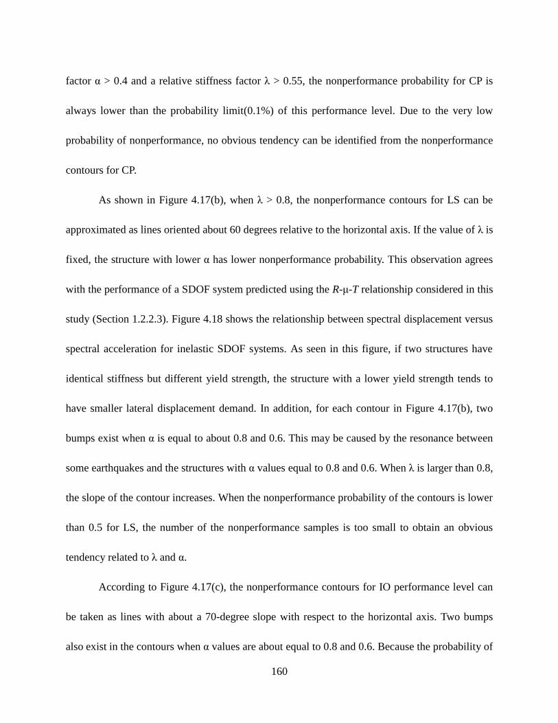
160

factor α > 0.4 and a relative stiffness factor λ > 0.55, the nonperformance probability for CP is

always lower than the probability limit(0.1%) of this performance level. Due to the very low

probability of nonperformance, no obvious tendency can be identified from the nonperformance

contours for CP.

As shown in Figure 4.17(b), when λ > 0.8, the nonperformance contours for LS can be

approximated as lines oriented about 60 degrees relative to the horizontal axis. If the value of λ is

fixed, the structure with lower α has lower nonperformance probability. This observation agrees

with the performance of a SDOF system predicted using the R-μ-T relationship considered in this

study (Section 1.2.2.3). Figure 4.18 shows the relationship between spectral displacement versus

spectral acceleration for inelastic SDOF systems. As seen in this figure, if two structures have

identical stiffness but different yield strength, the structure with a lower yield strength tends to

have smaller lateral displacement demand. In addition, for each contour in Figure 4.17(b), two

bumps exist when α is equal to about 0.8 and 0.6. This may be caused by the resonance between

some earthquakes and the structures with α values equal to 0.8 and 0.6. When λ is larger than 0.8,

the slope of the contour increases. When the nonperformance probability of the contours is lower

than 0.5 for LS, the number of the nonperformance samples is too small to obtain an obvious

tendency related to λ and α.

According to Figure 4.17(c), the nonperformance contours for IO performance level can

be taken as lines with about a 70-degree slope with respect to the horizontal axis. Two bumps

also exist in the contours when α values are about equal to 0.8 and 0.6. Because the probability of

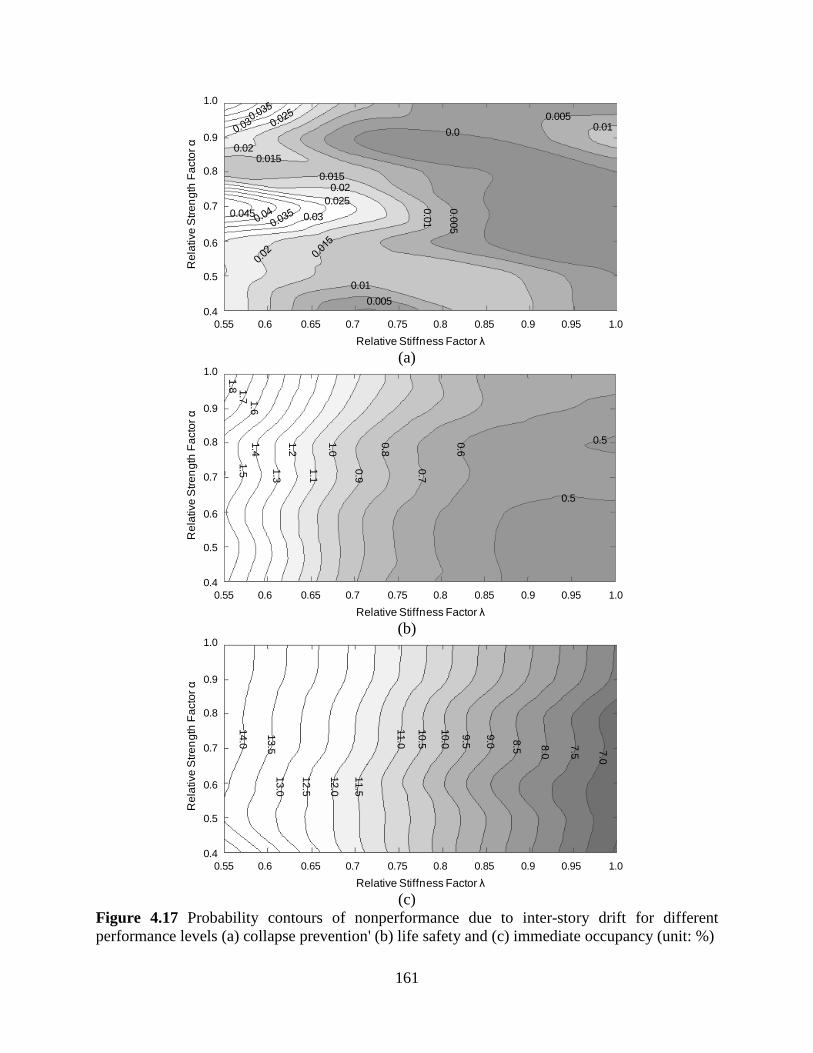
161

(a)

(b)

(c)

Figure 4.17 Probability contours of nonperformance due to inter-story drift for different

performance levels (a) collapse prevention' (b) life safety and (c) immediate occupancy (unit: %)

1.0

0.9

0.8

0.7

0.6

0.5

0.4

0.55 1.00.6 0.7 0.8 0.90.65 0.75 0.85 0.95

0.01

0.0

05

0.0

1


Re

lative

Str

en

gth

Fa

cto

r α

0.0

0.005

0.005

0.01

0.0150.02

0.03

0.025

0.045

0.0150.02

1.0

0.9

0.8

0.7

0.6

0.5

0.4

0.55 1.00.6 0.7 0.8 0.90.65 0.75 0.85 0.95

0.6

1.8

0.5

1.7


Re

lative

Str

en

gth

Fa

cto

r α

0.5

1.6

1.5

1.4

1.3

1.2

1.1

1.0

0.9

0.7

0.8

1.0

0.9

0.8

0.7

0.6

0.5

0.4

0.55 1.00.6 0.7 0.8 0.90.65 0.75 0.85 0.95

7.0

7.5

9.0 8.5 8.0

9.5

11.0

10.5

11.5

12.5

12.0

13.0

10.0


Re

lative

Str

en

gth

Fa

cto

r α

14.0

13.5

162

Figure 4.18 Deformation demand of inelastic SDOF systems with identical stiffness but

different yield strength

nonperformance at IO performance level is higher than the other performance levels, the

tendency of the contours is clearer. For both LS and IO performance levels shown in Figures

4.17(b) and 4.17(c), the nonperformance probability due to inter-story drift is affected mainly by

the relative stiffness factor λ rather than the relative strength factor α. For the structures with an

identical λ, the nonperformance probability due to inter-story drift is generally reduced with the

decrease in α.

Figure 4.19 shows the contours of nonperformance caused by excessive plastic hinge

rotation. In Figure 4.19(a) for CP, when λ < 0.7 and 0.9 < α < 1.0, or λ < 0.7 and 0.55 < α < 0.65,

the nonperformance contours can be approximated as vertical lines. This reflects that, in these

areas of λ and α, nonperformance probability is affected mainly by λ. When λ < 0.7 and 0.75 < α

< 0.9, or λ < 0.7 and 0.4 < α < 0.55, the nonperformance contours can be taken as lines with a

Sa

Sd

A

B

C

T

Elastic demand

spectrum

Bilinear

capacityspectra

Set of intersections between the capacity and

demand spectra with different yield strength

Inelastic demand

spectrum

C’

B’

163

(a)

(b)

(c)

Figure 4.19 Probability contours of nonperformance due to plastic hinge rotation for different

performance levels (a) collapse prevention; (b) life safety and (c) immediate occupancy (unit: %)

1.0

0.9

0.8

0.7

0.6

0.5

0.4

0.55 1.00.6 0.7 0.8 0.90.65 0.75 0.85 0.95

0.02

0.0

8

0.0

7

0.0

9

0.1

0

0.1

1

0.1

2 0.0

6


Re

lative

Str

en

gth

Fa

cto

r α

0.02

0.02

0.05

0.0

80.0

7

0.0

90.1

00.1

10.1

2

0.0

60.0

5

0.0

40.0

3

0.1

60.1

50.1

40.1

3

1.0

0.9

0.8

0.7

0.6

0.5

0.4

0.55 1.00.6 0.7 0.8 0.90.65 0.75 0.85 0.95

0.300.5

0

0.4

5

0.5

5

0.6

5

0.6

0

0.7

0

0.4

0


Re

lative

Str

en

gth

Fa

cto

r α

0.35

0.35

0.40

0.450.9

0

0.8

5 0.8

0

0.7

5

0.450.60

0.550.50

1.0

0.9

0.8

0.7

0.6

0.5

0.4

0.55 1.00.6 0.7 0.8 0.90.65 0.75 0.85 0.95


Re

lative

Str

en

gth

Fa

cto

r α

4.0

4.55.0

5.5

6.06.5

7.0

6.5

7.5

8.0

10.510.0

9.09.5

8.5

11.0

164

negative 45-degree slop with respect to the horizontal axis. Under this condition, if the value of λ

is fixed, the nonperformance probability increase with the decrease of α. This indicates that to

obtain an identical nonperformance probability, the structure can be designed based on higher α

but lower λ, or based on lower α but higher λ. When λ < 0.7 and 0.65 < α < 0.75, the

nonperformance contour can be approximated as lines with positive slope. This tendency shows

that the structure designed with lower values of both λ and α would have an identical

nonperformance probability to those with higher λ and α if λ < 0.7 and 0.65 < α < 0.75. When λ

is more than 0.7 and α is less than 0.6, the nonperformance contours have about 45-degree angle

with respect to the horizontal axis. Under this condition, if the value of λ is fixed,

nonperformance probability increases with the decrease of α. For the other contours with very

low nonperformance probability (0.02%), no obvious tendency can be identified. In Figure

4.19(a), especially for λ < 0.7, the feature of the contours of nonperformance due to plastic hinge

rotation is similar to that due to inter-story drift shown in Figure 4.19(b). This could be because

plastic hinge rotation is governed by inter-story drift under large lateral deformation.

As shown in Figure 4.19(c), the nonperformance contour for IO performance level is

affected mainly by α instead of λ. When 0.9 < α < 1.0 and 0.55 < λ < 0.85, the nonperformance

contours can be approximated into lines with about 20-degree slope with respect to the horizontal

axis. The slope increases with the value of λ. In two areas, one 0.9 < α < 1.0 and 0.85 < λ < 1.0,

the other with 0.4 < α < 0.6 and 0.7 < λ < 0.87, the nonperformance contours can be

approximated as lines oriented about 30 degrees relative to the horizontal axis. In these two areas,

165

if the value of λ is fixed, the nonperformance probability increases with the reduction of α. The

other contours in Figure 4.19(c) can be taken as horizontal lines, indicating that the probability

nonperformance evaluated based only on plastic hinge is governed by α.

In Figure 4.19(b), if λ < 0.8 and α > 0.5, the nonperformance contours for LS can be

approximated into lines oriented about 40 degrees relative to the horizontal axis. Two bumps

exist on these contours when the values of α are about equal to 0.6 and 0.8. If the value of λ is

fixed, the nonperformance probability is reduced with the increase of α. If λ < 0.55 and 0.4 < α <

0.5, the tendency of the contours are similar to those for λ < 0.8 and α > 0.5, but the slope is

decreased from 40 degrees to 30 degrees. For the aforementioned two cases, both λ and α affect

the nonperformance contours. This is because the number of plastic hinges and magnitude of

plastic hinge rotation for LS is between those for CP and IO; accordingly, both inter-story drift

and relative strength factor α affect the nonperformance contours. If 0.7 < λ < 0.83 and 0.4 < α <

0.5, the contours are almost vertical. In this area, the nonperformance probability is affected

mainly by λ rather than α. If λ > 0.8, a clear tendency cannot be identified due to the very low

nonperformance probability.

Figure 4.20 shows the probability contours of nonperformance due to either plastic hinge

rotation or inter-story drift. The contours depends on the nonperformance probability due to

plastic hinge rotation or inter-story drift, whichever controls. As shown in Figure 4.20(a), the

nonperformance contours for CP are very similar to those shown in Figure 4.19(a) for CP. This is

because the nonperformance probability due to inter-story drift is much lower than that due to

166

(a)

(b)

(c)

Figure 4.20 Probability contours of nonperformance due to either inter-story drift or plastic

hinge rotation for different performance levels (a) collapse prevention; (b) life safety; and (c)

immediate occupancy (unit: %)

1.0

0.9

0.8

0.7

0.6

0.5

0.4

0.55 1.00.6 0.7 0.8 0.90.65 0.75 0.85 0.95

0.0

3


Re

lative

Str

en

gth

Fa

cto

r α

0.02

0.02

0.020.01

0.03

0.1

10.1

00.0

90.0

80.0

70.0

60.0

50.0

4

0.1

50.1

40.1

30.1

2

0.1

6

1.0

0.9

0.8

0.7

0.6

0.5

0.4

0.55 1.00.6 0.7 0.8 0.90.65 0.75 0.85 0.95

0.70.8

1.0

0.9


Re

lative

Str

en

gth

Fa

cto

r α

0.6

0.7

0.71.5

1.4

1.3

1.2

1.1

1.6

1.7

1.8

1.0

0.9

0.8

0.7

0.6

0.5

0.4

0.55 1.00.6 0.7 0.8 0.90.65 0.75 0.85 0.95

8.0

8.51

0.0

9.5

9.01

0.51

2.0

11.5

12.5

13.5

12.0

14.0

11.0


Re

lative

Str

en

gth

Fa

cto

r α

167

plastic hinge rotation.

When α is more than 0.6, the nonperformance contours for LS shown in Figure 4.20(b)

are similar to those due to inter-story drift alone (Figure 4.17(b)). This is because, when α > 0.6,

the nonperformance probability due to inter-story drift alone (Figure 4.17(b)) is at least 50%

higher than that due to plastic hinge rotation only (Figure 4.19(b)). When α < 0.6, the difference

of nonperformance probability between the two types of contours becomes small, and the slope

angle of the contours due to plastic hinge only is much smaller than that due to inter-story drift

only. Therefore, when α < 0.6, the contours due to either plastic hinge rotation or inter-story drift

shown in Figure 4.20(b) are similar to those due to plastic hinge rotation only (Figure 4.19(b)).

When the α is about equal to 0.6 and 0.8, two bumps exist in the contours shown in Figure

4.20(b). In this figure, the contours corresponding to nonperformance probability greater than 0.7

shown can be divided into four segments for 0.4 < α < 0.6, 0.6 < α < 0.7, 0.7 < α < 0.8, and 0.8 <

α < 1.0. In the first and third segments, contours have 45- to 70-degree angles with respect to the

horizontal axis. If the value of λ is fixed, the nonperformance probability is reduced with the

increase of α. In the second and fourth segments, contours also have 45- to 70-degree angles with

respect to the horizontal axis but are in the opposite direction. Thus, if the value of λ is fixed, the

nonperformance probability increases with α. In all segments, the angle between the contours

and the horizontal axis is reduced with the increase of λ.

The nonperformance contours due to either plastic hinge rotation or inter-story drift for

IO are shown in Figure 4.20(c). When α > 0.6, the contours are similar to those due to inter-story

168

drift only because the nonperformance probability due to inter-story drift alone is much higher

than that due to plastic hinge rotation alone. When α < 0.6, the difference in nonperformance

probability between the two types of contours shown in Figures 4.17(c) and 4.19(c) becomes less.

The contours of nonperformance due to inter-story drift only and those due to plastic hinge

rotation only for IO are affected respectively by λ and α. Thus, as shown in Figure 4.20(c), the

contours of nonperformance based on both inter-story drift and plastic hinge rotation affected by

both λ and α when α < 0.6. In general, the contours in Figure 4.20(c) can be separately described

by two segments based on the values of α: (1) 0.6 < α < 1.0 and (2) 0.4 < α < 0.6. In the first

segment, the contours are almost vertical, implying that the nonperformance probability is

primarily affected by λ rather than α. In the second segment, the contours can be approximated

into lines with a 40-degree slope with respect to the horizontal axis. If the value of λ is fixed, the

nonperformance probability increases with the reduction of α. This tendency reflects that, with

the same nonperformance probability, a structure can be designed based on higher λ but lower α,

or higher α but lower λ.

As shown in Table 4.4, the nonperformance probability limits suggested for CP, LS and

IO performance levels are 0.1%, 1%, 10%, respectively. Figures 4.21 summarizes the

nonperformance contours corresponding to these limits. If a structure is designed based on the

values of λ and α at the point located on the right side of a contour, the nonperformance

probability is lower than the nonperformance probability limits represented by this contour.

Figure 4.21(a) shows the nonperformance probability limits based on inter-story drift

169

(a)

(b)

(c)

Figure 4.21 Nonperformance contours due to (a) inter-story drift; (b) plastic hinge rotation; and

(c) either plastic hinge rotation or inter-story drift (unit: %)

10

10

1

1

0.55 0.6 0.65 0.7 0.75 0.8 0.85 0.9 0.95 10.4

0.5

0.6

0.7

0.8

0.9

11.0

0.9

0.8

0.7

0.6

0.5

0.4

0.55 1.00.6 0.7 0.8 0.90.65 0.75 0.85 0.95


Re

lative

Str

en

gth

Fa

cto

r α

IOLS γ/[γ] > 1

101

0.1

0.1

0.55 0.6 0.65 0.7 0.75 0.8 0.85 0.9 0.95 10.4

0.5

0.6

0.7

0.8

0.9

11.0

0.9

0.8

0.7

0.6

0.5

0.4

0.55 1.00.6 0.7 0.8 0.90.65 0.75 0.85 0.95


Re

lative

Str

en

gth

Fa

cto

r α

IO

LS

CP

θ/[θ] > 1

10

10

1

1

0.1

0.1

0.55 0.6 0.65 0.7 0.75 0.8 0.85 0.9 0.95 10.4

0.5

0.6

0.7

0.8

0.9

11.0

0.9

0.8

0.7

0.6

0.5

0.4

0.55 1.00.6 0.7 0.8 0.90.65 0.75 0.85 0.95


Re

lative

Str

en

gth

Fa

cto

r α

10

IOLSCP

θ/[θ] > 1

orγ/[γ] > 1

170

only. The nonperformance probability for structures within the range of λ and α is always lower

than the limit for CP; thus, only the nonperformance contours corresponding to the limit of LS

and IO are drawn. The nonperformance probability limit for IO performance level is on the right

side. Therefore, it controls the feasible region of λ and α. If a structure is designed based on λ

larger than 0.84 and α larger than 0.4, then the nonperformance probability due to inter-story

drift satisfies all the nonperformance probability limits for three performance levels. Because the

contour for IO has about 80-degree angle measured from the horizontal axis, if the structure is

designed based on a low value of α such as 0.4, the feasible λ can be reduced to 0.78.

Figure 4.21(b) shows the nonperformance probability limits based on plastic hinge

rotation only. If a structure is designed with λ > 0.74 and α > 0.4, the nonperformance probability

limit for IO performance level controls the feasible region of λ and α, and the nonperformance

probability is lower than the limits for all three performance levels. If a structure is designed with

α > 0.45, the nonperformance probability limit for CP performance level controls the feasible

region of λ and α. In this condition, the feasible λ can be reduced to 0.65 while the structure can

still satisfy the nonperformance probability limit for all three performance levels.

As shown in Figure 4.21(c), the nonperformance probability limit for IO performance

level controls the feasible region of λ and α. If a structure is designed with λ > 0.85 and α > 0.6,

then the nonperformance probability based on both plastic hinge rotation and inter-story drift is

always lower than the limits for all three performance levels. The contour for IO performance

level has a 40-degree angle with respect to the horizontal axis. Therefore, if a structure is

171

designed with 0.4 < α < 0.6 and this structure is expected to satisfy the nonperformance

probability limits for all performance levels, the value of λ shall be increased from 0.85 to 1.0.

172

CHAPTER 5

SUMMARY AND CONCLUSIONS

5.1 Summary

The overall goal of this study is to develop an optimal performance-based seismic design

(PBSD) method for multi-story RC moment frames. This method is expected to have low

computational cost, and can be practically implemented by the U.S. design practice. To achieve

this goal, four tasks are completed: (1) developing a simplified optimal PBSD procedure that

incorporates the latest criteria of structural performance of RC frame buildings and can be

practically implemented by design engineers; (2) applying the proposed optimal PBSD method

to a prototype structure to investigate the efficiency of this method on cost saving; (3) examining

whether the optimal design derived from Task 2 can satisfy the requirements of the selected

performance levels under multiple hazard levels; and (4) performing structural reliability

analyses on the optimal structure, original structure, and other structures with different flexural

strength and stiffness to investigate how these factors affect the nonperformance probability of

RC moment frames.

For the first task, an optimal PBSD method based on capacity spectrum method is

developed for multi-story RC moment frames. This method minimizes the total construction cost,

and ensure that the optimized frame satisfies the deformation constraints for multiple selected

performance levels under different hazard levels. The proposed method simplifies the numerous

173

optimal variables into only two overall system variables normalized based on the original design:

a relative stiffness factor and a relative strength factor. A two-step optimal procedure is adopted

in this method. The feasible region boundary in the domain composed by the relative strength

factor and the relative stiffness factor is determined. The feasible region boundary is transformed

from the relative strength and stiffness factor domain to the material consumption domain. Then

the optimal design in the domain composed by the consumption of concrete and reinforcement is

determined.

To obtain the feasible region boundary in the first step, a convenient mathematical

iteration method based on the results of a single pushover analysis is proposed to search the

minimum relative stiffness for a given relative strength factor level. The feasible region

boundary is composed by the minimum relative stiffness factors for different levels of relative

strength factors. To obtain the optimal design in the second step, nonlinear programming method

is used to search the optimal solution of the problem with a linear objective function and a

convex feasible region.

For the second task, the proposed optimal PBSD method is applied to a six-story four-bay

RC prototype structure. The structure is first designed based on the conventional force-based

seismic design method as an initial design. The proposed optimal PBSD method is applied to

obtain the feasible region boundary in the relative strength and stiffness factor domain, and the

optimal design in the material consumption domain. The construction cost of the optimal design

is derived and compared with that of the original design.

174

For the third task, the nonlinear responses of the optimal and original structures are

determined from nonlinear dynamic analyses. The average structural responses under ten scaled

earthquake records are evaluated. These ten records are scaled according to the design spectra of

three selected hazard levels. The nonlinear responses of the optimal and original structures for

these three hazard levels are examined by the preselected performance limits.

For the fourth task, structural reliability analyses are performed on the original and

optimal structures by considering seven types of uncertainties in external loads, strength and

stiffness used to define the structural model, and performance-based limits. Latin Hypercube

sampling method is used to select the discrete values of the random variables, and combines

these discrete model parameters to create 8000 structure model samples for both the optimal and

the original structures. For each sample, nonlinear dynamic analysis is performed to obtain the

normalized nonlinear structural deformations defined by inter-story drift and plastic hinge

rotation. The normalized nonlinear structural deformation reflects whether the sample satisfies a

target performance level. The normalized nonlinear structural deformations of 8000 samples are

used to establish fragility curves and calculate the nonperformance probabilities of the optimal

and original structures. Such a reliability analysis method is the extended to on other 26

structures with various relative strength and stiffness factors different from the optimal and

original structures. The nonperformance probabilities of the total 28 structures are used to

establish the nonperformance contours to investigate how the relative strength and stiffness

factors affect the nonperformance probability.

175

5.2 Conclusions

The following conclusion can be reached based on the optimal result of the prototype

structure used in this study by applying the proposed optimal PBSD method:

(1) An optimal performance-based seismic design method for multi-story RC moment

frames is proposed in this study based on the capacity spectrum method. The proposed method

requires comparatively low computational cost.

(2) Compared with the conventional strength-based design, the proposed optimal PBSD

method can lead to a 30% reduction in the needed flexural strength for the beams and the

columns, a 26% reduction in this cross-sectional area, and about 20% reduction in the overall

cost.

(3) If both inter-story drift and plastic hinge rotation are used to evaluate the structural

nonlinear response, the optimal result for the prototype building is controlled by inter-story drift

limit for the Life Safety performance level under rare earthquakes. If only plastic hinge rotation

is used to measure structural performance, the construction cost can be further reduced, and the

optimal design would be controlled by the limit for the Life Safety performance level under rare

earthquakes. The limits of inter-story drift and plastic hinge rotation for Collapse Prevention

performance level do not control the optimal result.

(4) Nonlinear dynamic analyses indicate that, in general, the optimal result derived from

the proposed optimal PBSD method can satisfy the deformation limits of multiple performance

levels under different hazard levels. The plastic hinge rotation demand are farther less than the

176

limits for all three performance levels.

(5) Structural reliability analyses indicate that, in general, the structural probability of

nonperformance evaluated using inter-story drift is sensitive the relative stiffness factor rather

than the relative strength factor. The probability of nonperformance due to plastic hinge rotation

for Immediate Occupancy performance level is sensitive to relative strength factor instead of

relative stiffness factor. The probability of nonperformance due to plastic hinge rotation for Life

Safety performance level is affected by both relative strength factor and stiffness.

(6) When both plastic hinge rotation and inter-story drift are used to limit the response of

structure, the probability for Collapse Prevention performance level is affected mainly by plastic

hinge rotation. The probability of nonperformance for Life Safety and Immediate Occupancy

performance levels is affected by both plastic hinge rotation and inter-story drift. The effect

caused by inter-story drift is higher than plastic hinge rotation.

(7) To design a structure satisfying the probability limit of nonperformance due to

inter-story drift, the relative stiffness factor λ shall be larger than 0.84 and the relative strength

factor α shall be larger than 0.4. To design a structure satisfying the probability limit of

nonperformance due to plastic hinge rotation, λ can be larger than 0.75 and the α can be larger

than 0.4; otherwise, λ can be larger than 0.65 and the α can be larger than 0.45. To design a

structure satisfying the probability limit of nonperformance due to either plastic hinge rotation or

inter-story drift, λ shall be larger than 0.85 and the α shall be larger than 0.6.

177

5.3 Suggestions

The followings are future research suggestions:

(1) The proposed optimal PBSD method can be extended by using more optimal

variables. This can be achieved by assigning different relative stiffness and strength factors for

each story to optimize the stiffness and strength of the elements. A better optimal design can be

obtained based in this way, which however requires additional optimal algorithm and

computational cost.

(2) The proposed method can be applied to RC moment frames with different geometries

considering the effect of higher vibration modes to further support the conclusions derived from

the prototype structure in this study.

(3) To obtain an realistic flexural response of elements, fiber elements can be used to

establish the structural model instead of using the plastic concentrated elements in this study.

However, this will cause a large additional computational cost in structural analyses.

(4) The required minimum sampling number shall be determined in order to identify a

clear tendency of contours, when the nonperformance probability is less than 0.1%.

178

REFERENCES

Abrahamson, N. A., Silva, W. J., and Kamai, R. (2014). Summary of the ASK14 ground motion

relation for active crustal regions. Earthquake Spectra, 30(3), 1025-1055.

ACI (American Concrete Institute). (2014). Building Code Requirements for Structural Concrete

and Commentary. (ACI 318-14). American Concrete Institute, Farmington Hills, MI,

2014.

Antoniou, S. and Pinho, R. (2004). Development and verification of a displacement-based

adaptive pushover procedure. Journal of Earthquake Engineering, 8(5), 643-661.

ASCE (American Society of Civil Engineers). (2010). Minimum Design Loads for Buildings and

Other Structures. (ASCE/SEI 7-10), American Society of Civil Engineers, Reston, VA,

2010.

ASCE (American Society of Civil Engineers). (2007). Seismic Rehabilitation of Existing

Buildings. (ASCE/SEI 41-06), American Society of Civil Engineers, Reston, VA, 2007.

ASCE (American Society of Civil Engineers). (2014). Seismic Rehabilitation of Existing

Buildings. (ASCE/SEI 41-13), American Society of Civil Engineers, Reston, VA, 2014.

ATC (Applied Technology Council). (1996). Seismic Evaluation and Retrofit of Concrete

Buildings. (ATC-40), Applied Technology Council, California Seismic Safety

Commission: Redwood City, CA, 1996.

Ayyub, B. M. and McCuen, R. H. (2016). Probability, statistics, and reliability for engineers and

scientists. CRC press, 2016.

Baker, J. W. (2015). Efficient analytical fragility function fitting using dynamic structural

analysis. Earthquake Spectra, 31(1), 579-599.

Bertero, R. D. and Bertero, V. V. (2002). Performance‒based seismic engineering: the need for a

reliable conceptual comprehensive approach. Earthquake Engineering and Structural

Dynamics, 31(3), 627-652.

Boore, D. M., Stewart, J. P., Seyhan, E., and Atkinson, G. M. (2014). NGA-West2 equations for

179

predicting PGA, PGV, and 5% damped PSA for shallow crustal earthquakes. Earthquake

Spectra, 30(3), 1057-1085.

Bracci, J. M., Kunnath, S. K., and Reinhorn, A. M. (1997). Seismic performance and retrofit

evaluation of reinforced concrete structures. Journal of Structural Engineering, 123(1),

3-10.

Bulleit, W. M. (2008). Uncertainty in structural engineering. Practice Periodical on Structural

Design and Construction, 13(1), 24-30.

Campbell, K. W. and Bozorgnia, Y. (2014). NGA-West2 ground motion model for the average

horizontal components of PGA, PGV, and 5% damped linear acceleration response

spectra. Earthquake Spectra, 30(3), 1087-1115.

Chan, C. M. and Zou, X. K. (2004). Elastic and inelastic drift performance optimization for

reinforced concrete buildings under earthquake loads. Earthquake Engineering and

Structural Dynamics, 33(8), 929-950.

Chiou, B. S. J. and Youngs, R. R. (2014). Update of the Chiou and Youngs NGA model for the

average horizontal component of peak ground motion and response spectra. Earthquake

Spectra, 30(3), 1117-1153.

Chopra, A. K. (2017). Dynamics of structures. theory and applications to. Earthquake

Engineering, 2017.

Chopra, A. K. and Goel, R. K. (1999). Capacity-demand-diagram methods based on inelastic

design spectrum. Earthquake Spectra, 15(4), 637-656.

Cowper G. R. (1996) The shear coefficient in Timoshenko's beam theory. Journal of Applied

Mechanics, 33(2), 335-340.

Deierlein, G. G., Reinhorn, A. M., and Willford, M. R. (2010). Nonlinear structural analysis for

seismic design. NEHRP Seismic Design Technical Brief, 4, 1-36.

Ellingwood, B. (1980). Development of a probability based load criterion for American National

Standard A58: Building code requirements for minimum design loads in buildings and

other structures (Vol. 13). US Department of Commerce, National Bureau of Standards,

180

1980.

Ellingwood, B. R. (2003). Toward load and resistance factor design for fiber-reinforced polymer

composite structures. Journal of Structural Engineering, 129(4), 449-458.

Elwood, K. J. and Eberhard, M. O. (2009). Effective stiffness of reinforced concrete columns.

ACI Structural Journal, 106(4), 1-5.

Elwood, K. J., Matamoros, A. B., Wallace, J. W., Lehman, D. E., Heintz, J. A., Mitchell, A. D.,

and Moehle, J. P. (2007). Update to ASCE/SEI 41 concrete provisions. Earthquake

Spectra, 23(3), 493-523.

Fajfar, P. (1999). Capacity spectrum method based on inelastic demand spectra. Earthquake

Engineering and Structural Dynamics, 28(9), 979-993.

Fajfar, P. (2000). A nonlinear analysis method for performance-based seismic design. Earthquake

Spectra, 16(3), 573-592.

Fajfar, P. and Gaspersic, P. (1996). The N2 method for the seismic damage analysis of RC

buildings. Earthquake Engineering and Structural Dynamics, 25(1), 31-46.

Fajfar, P. (2002). Structural analysis in earthquake engineering–a breakthrough of simplified

non-linear methods. 12th European Conference on Earthquake Engineering, 2002.

Fajfar, P. and Fischinger, M. (1988). N2-A method for non-linear seismic analysis of regular

buildings. Proceedings of the Ninth World Conference in Earthquake Engineering. 5,

111-116.

FEMA (Federal Emergency Management Agency). (1997). NEHRP guidelines for the seismic

rehabilitation of buildings. (FEMA 273), Federal Emergency Management Agency,

Washington, D.C, 1997.

FEMA (Federal Emergency Management Agency). (1997). NEHRP commentary on the

guidelines for the seismic rehabilitation of buildings. (FEMA 274), Federal Emergency

Management Agency, Washington, D.C, 1997

FEMA (Federal Emergency Management Agency). (2000). Prestandard and commentary for the

seismic rehabilitation of buildings. (FEMA 356), Federal Emergency Management

181

Agency Washington, D.C, 2000.

Fragiadakis, M., and Papadrakakis, M. (2008). Performance‒based optimum seismic design of

reinforced concrete structures. Earthquake Engineering & Structural Dynamics, 37(6),

825-844.

Freeman, S. A. (1998). Development and use of capacity spectrum method. The 6th US National

Conference on Earthquake Engineering/EERI, Seattle, Washington, 1998.

Ganzerli, S., Pantelides, C. P., and Reaveley, L. D. (2000). Performance-based design using

structural optimization. Earthquake Engineering and Structural Dynamics, 29(11),

1677-1690.

Gaxiola-Camacho, J. R., Azizsoltani, H., Villegas-Mercado, F. J., and Haldar, A. (2017). A novel

reliability technique for implementation of Performance-Based Seismic Design of

structures. Engineering Structures, 142, 137-147.

Ghobarah, A. (2001). Performance-based design in earthquake engineering: state of development.

Engineering Structures, 23(8), 878-884.

Gholizadeh, S. (2015). Performance-based optimum seismic design of steel structures by a

modified firefly algorithm and a new neural network. Advances in Engineering Software,

81, 50-65.

Gholizadeh, S. and Moghadas, R. K. (2014). Performance-based optimum design of steel frames

by an improved quantum particle swarm optimization. Advances in Structural

Engineering, 17(2), 143-156.

Goel, S. C. and Chao, S. H. (2008). Performance-based plastic design: earthquake-resistant steel

structures. International Code Council, 2008.

Goel, S. C., Liao, W. C., and Reza Bayat, M. (2010). Performance-based plastic design (PBPD)

method for earthquake-resistant structures: an overview. The Structural Design of Tall

and Special Buildings, 19(1-2), 115-137.

Gong, Y. (2003). Performance-based design of building frameworks under seismic loading. PhD

thesis, University of Waterloo, Waterloo, Canada, 2003.

182

Gong, Y., Xu, L., and Grierson, D. E. (2005). Performance-based sensitivity analysis of steel

moment frameworks under seismic loading. International Journal of Numerical Methods

in Engineering, 63(9), 1229-1249.

Grierson, D. E., Gong, Y., and Xu, L. (2006). Optimal performance-based seismic design using

modal pushover analysis. Journal of Earthquake Engineering, 10(1), 73-96.

Gupta, B. and Kunnath, S. K. (2000). Adaptive spectra-based pushover procedure for seismic

evaluation of structures. Earthquake Spectra, 16(2), 367-392.

Hajirasouliha, I., Asadi, P., and Pilakoutas, K. (2012). An efficient Performance-based seismic

design method for reinforced concrete frames, Earthquake Engineering and Structural

Dynamics, 41(4), 663-679.

Hettmansperger, T. P. and McKean, J. W. (1978). Statistical inference based on ranks.

Psychometrika, 43(1), 69-79.

Huang, M. F., Li, Q., Chan, C. M., Lou, W. J., Kwok, K. C., and Li, G. (2015).

Performance-based design optimization of tall concrete framed structures subject to wind

excitations. Journal of Wind Engineering and Industrial Aerodynamics, 139, 70-81.

Huyse, L., Chen, R., and Stamatakos, J. A. (2010). Application of generalized Pareto distribution

to constrain uncertainty in peak ground accelerations. Bulletin of the Seismological

Society of America, 100(1), 87-101.

Ibarra, L. F., Medina, R. A., and Krawinkler, H. (2005). Hysteretic models that incorporate

strength and stiffness deterioration. Earthquake Engineering and Structural Dynamics,

34(12), 1489-1511.

Ibarra, L. F. and Krawinkler, H. (2005). Global collapse of frame structures under seismic

excitations. Berkeley, CA: Pacific Earthquake Engineering Research Center, 2005.

Idriss, I. M. (2014). An NGA-West 2 empirical model for estimating the horizontal spectral

values generated by shallow crustal earthquakes. Earthquake Spectra, 30(3), 1155-1177.

Iervolino, I. and Cornell, C. A. (2008). Probability of occurrence of velocity pulses in

near-source ground motions. Bulletin of the Seismological Society of America, 98(5),

183

2262-2277.

Iman, R. L. and Conover, W. J. (1980). Small sample sensitivity analysis techniques for

computer models, with an application to risk assessment. Communications in

Statistics-theory and Methods, 9(17), 1749-1842.

Kalkan, E., and Kunnath, S. K. (2007). Assessment of current nonlinear static procedures for

seismic evaluation of buildings. Engineering Structures, 29(3), 305-316.

Kaveh, A., Azar, B. F., and Hadidi, A. (2010). Performance-based seismic design of steel frames

using ant colony optimization. Journal of Constructional Steel Research, 66(4), 566-574.

Kaveh, A., Laknejadi, K., and Alinejad, B. (2012). Performance-based multi-objective

optimization of large steel structures. Acta Mechanica, 223(2), 355-369.

Kaveh, A. and Nasrollahi, A. (2014). Performance-based seismic design of steel frames utilizing

charged system search optimization. Applied Soft Computing, 22, 213-221.

Khatibinia, M., Fadaee, M. J., Salajegheh, J., and Salajegheh, E. (2013). Seismic reliability

assessment of RC structures including soil–structure interaction using wavelet weighted

least squares support vector machine. Reliability Engineering and System Safety, 110,

22-33.

Kogut, G. F. and Chou, K. C. (2004). Partial resistance factor design on steel–concrete

beam-columns. Engineering Structures, 26(7), 857-866.

Krawinkler, H. (1992). Seismic design based on ductility and cumulative damage demand and

capacities. Nonlinear Seismic Analysis and Design of Reinforced Concrete Buildings,

23-39.

Krawinkler, H. (1999). Challenges and progress in performance-based earthquake engineering.

International Seminar on Seismic Engineering for Tomorrow–In Honor of Professor

Hiroshi Akiyama, 26.

Krawinkler, H., and Seneviratna, G. D. P. K. (1998). Pros and cons of a pushover analysis of

seismic performance evaluation. Engineering structures, 20(4-6), 452-464.

Kircher, C. A., Reitherman, R. K., Whitman, R. V., and Arnold, C. (1997). Estimation of

184

earthquake losses to buildings. Earthquake Spectra, 13(4), 703-720.

Kreslin, M. and Fajfar, P. (2012). The extended N2 method considering higher mode effects in

both plan and elevation. Bulletin of Earthquake Engineering, 10(2), 695-715.

Lee, J. O., Yang, Y. S., and Ruy, W. S. (2002). A comparative study on reliability-index and

target-performance-based probabilistic structural design optimization. Computers and

Structures, 80(3-4), 257-269.

Li, G., Lu, H., and Liu, X. (2010). A hybrid genetic algorithm and optimality criteria method for

optimum design of RC tall buildings under multi-load cases. The Structural Design of

Tall and Special Buildings, 19(6), 656-678.

Li, G. and Hu, H. (2014). Risk design optimization using many-objective evolutionary algorithm

with application to performance-based wind engineering of tall buildings. Structural

Safety, 48, 1-14.

Liang, Q. Q., Uy, B., and Steven, G. P. (2002). Performance-based optimization for strut-tie

modeling of structural concrete. Journal of Structural Engineering, 128(6), 815-823.

Lignos, D. G. and Krawinkler, H. (2012). Development and utilization of structural component

databases for performance-based earthquake engineering. Journal of Structural

Engineering, 139(8), 1382-1394.

Lignos, D. G. and Krawinkler, H. (2010). Deterioration modeling of steel components in support

of collapse prediction of steel moment frames under earthquake loading. Journal of

Structural Engineering, 137(11), 1291-1302.

Lignos, D. (2008). Sidesway collapse of deteriorating structural systems under seismic

excitations. Stanford university, 2008.

Liu, M., Burns, S. A., and Wen, Y. K. (2005). Multiobjective optimization for performance-based

seismic design of steel moment frame structures. Earthquake Engineering and Structural

Dynamics, 34(3), 289-306.

Liu, B. Q., Liu, M., and Li, Y. B. (2004). Research and development of performance-based

seismic design theory. The 13th World Conference on Earthquake Engineering,

185

Vancouver (BC), Canada, 2004.

McCormac, J. C. and Brown, R. H. (2015). Design of reinforced concrete. John Wiley and Sons,

2015.

Mechakhchekh, A. and Ghosn, M. (2007). Reliability-based procedure for developing load and

resistance factor seismic bridge design specifications. Transportation Research Record,

2028(1), 173-179.

Moehle, J. (1992). Displacement-based design of RC structures subjected to earthquakes.

Earthquake Spectra, 8(3), 403-428.

Moehle, J. P. (1996) Displacement-based seismic design criteria. 11th World Conference on

Earthquake Engineering, Acapulco, Mexico, 1996

Moharrami, H. and Grierson, D. E. (1993). Computer-automated design of reinforced concrete

frameworks. Journal of Structural Engineering, 119(7), 2036-2058.

Miranda, E. and Bertero, V. V. (1994). Evaluation of strength reduction factors for

earthquake-resistant design. Earthquake Spectra, 10(2), 357-379.

Möller, O., Foschi, R. O., Ascheri, J. P., Rubinstein, M., & Grossman, S. (2015). Optimization

for performance-based design under seismic demands, including social costs. Earthquake

Engineering and Engineering Vibration, 14(2), 315-328.

Möller, O., Foschi, R. O., and Quiroz, L. M. (2009). Structural optimization for

performance-based design in earthquake engineering: applications of neural networks.

Structural Safety, 31(6), 490-499.

Murakami, M. and Penzien, J. (1975). Nonlinear response spectra for probabilistic seismic

design and damage assessment of reinforced concrete structures. Earthquake Engineering

Research Center, University of California, 1975.

Nassar, A. A., Osteraas, J. D., and Krawinkler, H. (1992). Seismic design based on strength and

ductility demands. 10th World Conference on Earthquake Engineering, 10, 5861-5866.

Newmark, N. M. and Hall, W. J. (1982). Earthquake spectra and design. Earthquake Engineering

Research Institute, Berkeley, CA, 1982

186

Newmark, N. M., Hall, W. J. (1969). Seismic design criteria for nuclear reactor facilities. World

Conference of Earthquake Engineering, B-4. 37-50.

Park, Y. and Ang, A. (1985). Mechanistic seismic damage model for reinforced concrete. Journal

of Structural Engineering, 111(4), 722–739.

Park, H. G., Eom, T., and Lee, H. (2007). Factored modal combination for evaluation of

earthquake load profiles. Journal of Structural Engineering, 133(7), 956-968.

Paulay, T. and Priestley, M. J. N. (1992). Seismic design of reinforced concrete and masonry

buildings, Wiley-Interscience, New York, 1992.

Priestley, M. J. N., Calvi, G. M., and Kowalsky, M. J. (2007). Direct displacement-based seismic

design. 2005 New Zealand Society for Earthquake Engineering Conference, 33-43.

Priestley, M. J. N. (2000). Performance based seismic design. Bulletin of the New Zealand

Society for Earthquake Engineering, 33(3), 325-346.

Priestley, M. J. N., Kowalsky, M. J., Ranzo, G., and Benzoni, G. (1996). Preliminary

development of direct displacement-based design for multi-degree of freedom systems,

65th Annual SEAOC Convention, 47-66.

Priestley, M. J. N. and Park, R. (1987). Strength and ductility of concrete bridge columns under

seismic loading. Structural Journal, 84(1), 61-76.

Powell, G. H. (2008). Displacement-based seismic design of structures. Earthquake spectra,

24(2), 555-557.

Plevris, V. ed. (2012). Structural seismic design optimization and earthquake engineering:

formulations and applications: formulations and applications. IGI Global, 2012.

Rainer, J. H. and Karacabeyli, E. (2000). Performance of wood-frame construction in

earthquakes. The 12th World Conference on Earthquake Engineering, Auckland, New

Zealand (30), 1-8.

Rashedi, E., Nezamabadi-Pour, H., and Saryazdi, S. (2009). GSA: a gravitational search

algorithm. Information sciences, 179(13), 2232-2248.

187

Reinhorn, A. M. (1997). Inelastic analysis techniques in seismic evaluations. Seismic design

methodologies for the next generation of performance based seismic engineering of codes,

277-287.

Rwamamara, R., Simonsson, P., and Ojanen, J. (2010). Advantages of industrialized methods

used in small bridge construction. Annual Conference of the International Group for

Lean Construction, 569-579.

Sasani, M. (1998). A two-level-performance-based design of reinforced concrete structural walls.

6th US National Conference on Earthquake Engineering, EERI: Oakland, CA, 1998.

Schmit, L. A. and Farshi, B. (1974). Some approximation concepts for structural synthesis.

American Institute of Aeronautics and Astronautics Journal, 12(5), 692-699.

SEAOC (Structural Engineers Association of California). (1995). Performance Based Seismic

Engineering of Buildings. Sacramento, CA.

SEAOC (Structural Engineers Association of California) Seismology Committee. (2008). A brief

guide to seismic design factors. Structure Magazine, 30-32

Shooman, M. L. (1968). Reliability physics models. IEEE Transactions on Reliability, 17(1),

14-20.

Soegiarso, R. and Adeli, H. (1997). Optimum load and resistance factor design of steel

space-frame structures. Journal of Structural Engineering, 123(2), 184-192.

Soong, T. T. and Grigoriu, M. (1993). Random vibration of mechanical and structural systems.

NASA STI/Recon Technical Report, A 93.

Subramanian, N. (2010). Limiting reinforcement ratios for RC flexural members. Indian

Concrete Journal, 84(9), 71.

Sung, Y. C., Liao, W. I., and Yen, W. P. (2009). Performance-based concept on seismic evaluation

of existing bridges. Earthquake Engineering and Engineering Vibration, 8(1), 127-135.

Talatahari, S. (2013). Optimum performance-based seismic design of frames using metaheuristic

optimization algorithms. Metaheuristic applications in structures and infrastructures.

Elsevier, 419-37.

188

Talatahari, S., Hosseini, A., and Mirghaderi, S. R. (2014). Optimum performance-based seismic

design using a hybrid optimization algorithm. Mathematical Problems in Engineering,

2014.

Veletsos, A. S. and Newmark, N. M. (1960) Effect of inelastic behavior on the response of

simple systems to earthquake motions, The 2nd World Conference on Earthquake

Engineering, 2, 895–912.

Veletsos, A. S. and Newmark, N. M. (1964) Design procedures for shock isolation systems of

underground protective structures, 3, Response Spectra of Single-Degree-of-Freedom

Elastic and Inelastic Systems, Newmark Hansen and Associates Urbana.

Vidic, T., Fajfar, P., and Fischinger, M. (1994). Consistent inelastic design spectra: strength and

displacement. Earthquake Engineering and Structural Dynamics, 23(5), 507-521.

Welch, D. P., Sullivan, T. J., and Calvi, G. M. (2014). Developing direct displacement-based

procedures for simplified loss assessment in performance-based earthquake engineering.

Journal of Earthquake Engineering, 18(2), 290-322.

Xu, L., Gong, Y., and Grierson, D. E. (2006). Seismic design optimization of steel building

frameworks. Journal of Structural Engineering, 132(2), 277-286.

Yang, I. H. (2006). Uncertainty Analysis of Concrete Structures Using Modified Latin

Hypercube Sampling Method. International Journal of Concrete Structures and

Materials, 18(2E), 89-95.

Yazdani, H., Khatibinia, M., Gharehbaghi, S., and Hatami, K. (2016). Probabilistic

performance-based optimum seismic design of RC structures considering soil–structure

interaction effects. ASCE-ASME Journal of Risk and Uncertainty in Engineering Systems,

Part A: Civil Engineering, 3(2), G4016004.

Zameeruddin, M. and Sangle, K. K. (2016). Review on Recent developments in the

performance-based seismic design of reinforced concrete structures. Structures, 6,

119-133.

Zou, X. K. and Chan, C. M. (2005 a). An optimal resizing technique for seismic drift design of

concrete buildings subjected to response spectrum and time history loadings. Computers

189

and Structures, 83(19-20), 1689-1704.

Zou, X. K. and Chan, C. M. (2005 b). Optimal seismic performance-based design of reinforced

concrete buildings using nonlinear pushover analysis. Engineering Structures. 27(8),

1289-1302.

Zou, X. K., Chan, C. M., and Li, G. (2007). Multi-objective optimization for performance-based

design of reinforced concrete frames. Journal of structural engineering, 133(10),

1462-1474.

190

CURRICULUM VITAE

Graduate College


Chunyu Zhang

[email protected]

Education:

Bachelor of Science in Civil Engineering, Shenyang Jianzhu University, 2009

Master of Science in Civil Engineering, Shenyang Jianzhu University, 2012

Employment:

Coordinator of the evaluation and demonstration division

Ministry of Construction of China

March 2012 - April 2013

Beijing, China

Online instructor

Northeastern University, China

March 2012 - March 2010

Shenyang, China

Thesis Title:

Study of the seismic performance of high-strength concrete filled square steel tube column with

inner CFRP circular tube frame structures (2012)

Dissertation Title:

Performance-based Economical seismic design of multistory reinforced concrete frame buildings

and reliability assessment

Dissertation Examination Committee:

Chairperson, Dr. Ying Tian

Committee Member, Dr. Nader Ghafoori

Committee Member, Dr. Mohamed Kaseko

Committee Member, Dr. Samaan Ladkany

Graduate Faculty Representative, Dr. Mohamed Trabia

Publication:

Zhang, C., and Tian, Y. “Performance-based Optimal Seismic Design of Reinforced Concrete

Frame Buildings,” Engineering Structures, under review.

191

Wang, L., Tian, Y., Luo, W., Li, G., Zhang, S. and Zhang, C. “Experimental Study of Seismic

Performance of Axially Restrained Reinforced Concrete Frame Beams,” Journal of Structural

Engineering, accepted.

Li, G., Liu, D., Yang, Z., and Zhang, C. (2017). “Flexural Behavior of High Strength

Concrete-filled High Strength Square Steel Tube,” Journal of Constructional Steel Research, 128,

732-744.

Li, G., Qiu, Z., and Zhang, C. (2016). “Dynamic Time-history Analysis of High-strength

Concrete-filled Square Steel Tube Column with Inner CFRP Circular Tube Frame Structure,”

Journal of Shenyang Jianzhu University (Natural Science), in Chinese, 32(2), 216-224.

performance-based economical seismic design of multistory

Documents