performance assessment of seismic resistant steel structures · performance assessment of seismic...

Performance Assessment of Seismic Resistant

Steel Structures

Jordan Alesa Jarrett

Dissertation submitted to the faculty of the Virginia Polytechnic Institute and State

University in partial fulfillment of the requirements for the degree of

Doctor of Philosophy

In

Civil Engineering

Finley A. Charney, Chair

Matthew R. Eatherton

Cristopher D. Moen

Adrian Rodriguez-Marek

December 2, 2013

Blacksburg, VA

Keywords: Nonlinear Response History Analysis, FEMA P-58, FEMA P-695, ASCE 7,

Innovative Systems

Performance Assessment of Seismic Resistant Steel Structures

Jordan Alesa Jarrett

Abstract

This work stems from two different studies related to this performance assessment of seismic

resistant systems. The first study compares the performance of newly developed and traditional

seismic resisting systems, and the second study investigates many of the assumptions made

within provisions for nonlinear response history analyses.

In the first study, two innovative systems, which are hybrid buckling restrained braces and

collapse prevention systems, are compared to their traditional counterparts using a combination

of the FEMA P-695 and FEMA P-58 methodologies. Additionally, an innovative modeling

assumption is investigated, where moment frames are evaluated with and without the lateral

influence of the gravity system. Each system has a unique purpose from the perspective of

performance-based earthquake engineering, and analyses focus on the all intensity levels of

interest. The comparisons are presented in terms consequences, including repair costs, repair

duration, number of casualties, and probability of receiving an unsafe placard, which are more

meaningful to owners and other decision makers than traditional structural response parameters.

The results show that these systems can significantly reduce the consequences, particularly the

average repair costs, at the important intensity levels.

The second study focuses on the assumptions made during proposed updates to provisions for

nonlinear response history analyses. The first assumption investigated is the modeling of the

gravity system’s lateral influence, which can have significant effect on the system behavior and

should be modeled if a more accurate representation of the behavior is needed. The influence of

residual drifts on the proximity to collapse is determined, and this work concludes that a residual

drift check is unnecessary if the only limit state of interest is collapse prevention. This study also

finds that spectrally matched ground motions should cautiously be used for near-field structures.

The effects of nonlinear accidental torsion are also examined in detail and are determined to have

a significant effect on the inelastic behavior of the analyzed structure. The final investigation in

this study shows that even if a structure is designed per ASCE 7, it may not have the assumed

probability of collapse under the maximum considered earthquake when analyzed using FEMA

P-695.

iii

Acknowledgements

I would especially like to thank my advisor Dr. Finley Charney for the opportunity to work on

these interesting and challenging projects. I am eternally grateful for all his guidance, expertise,

and encouragement. I would also like to thank my Masters advisor, Dr. Paul Heyliger, for

inspiring me to get my Ph.D. in the first place. I am also indebted to my committee, Dr. Matthew

Eatherton, Dr. Cris Moen, and Dr. Rodriguez-Marek for their comments and suggestions

throughout this process.

I am also appreciative of my colleagues Francisco Flores, Andy Hardyneic, Johnn Judd, Ozgur

Atlayan and Reid Zimmerman for their contribution and collaboration. I would also like to

acknowledge the help provided by Clint Rex, Jim Sexton, Vickie Mouras, Jack Baker, and Curt

Haselton during the process of this research. I would furthermore like to thank the Charles E. Via

Fellowship Program, the Department of Civil and Environmental Engineering, and NIST grant

60ANB10D107 for funding my education.

This would not be possible without the support of my family, for which I am forever

appreciative. And finally, I want to thank all my friends from Colorado State University and

Virginia Tech for making the past ten and a half years an amazing experience. Go Rams and

Hokies!

iv

Table of Contents

Abstract ii

Acknowledgements iii

Table of Contents iv

List of Figures vii

List of Tables x

Chapter 1: Introduction 1

1.1. Overview and Purpose of Work 1

1.2. Dissertation Organization 4

1.3. Attribution 5

Chapter 2: Literature Review 6

2.1. Summary of Performance Based Earthquake Engineering Principles 6

2.2. Incremental Dynamic Analysis 7

2.2.1. Background 7

2.2.2 General Procedure of Incremental Dynamic Analysis 7

2.2.3 Applications of Incremental Dynamic Analysis 9

2.2.4. Alternative Methods to Incremental Dynamic Analyses 14

2.3. Fragility Curves 16

2.3.1. Introduction to Fragility Curves 16

2.3.2. Relationship between IDA and Fragility Curves 17

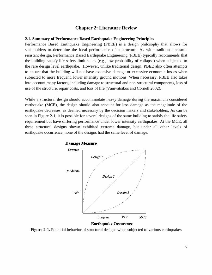
2.3.3. Background on Necessary Statistics 17

2.3.4. Building Fragility Curves 20

2.3.5. Application to FEMA P-695 21

2.3.6. Other Examples of Previous Fragility Analysis 22

2.3.7. Goodness of Fit Tests 25

2.3.8. Integrating Fragility with Seismic Hazard Curves 28

2.4. Background on ASCE 7 Nonlinear Dynamic Analysis Procedure 29

2.4.1. Methodology 29

2.4.2. Current Implementation 29

2.4.3. BSSC Proposed Updates 30

2.5. Background on FEMA P-695 Procedure 31

2.5.1. Full P-695 Methodology 31

2.5.2. Appendix F Methodology for Individual Structures 33

2.5.3. Current Implementation 34

2.6. Background on FEMA P-58 Procedure 35

2.6.1. Building Performance Modeling 36

2.6.2. Assessment Types 39

2.6.3. Ground Motion Selection and Scaling 40

2.6.4. Analyze Building Response 40

2.6.5. Performance Calculations 41

v

2.6.6. Consequence Results 43

2.6.7. Benefits of the FEMA P-58 Methodology from the Perspective of PBEE 45

2.7. Accidental Torsion in Dynamic Analyses 46

Chapter 3: “Comparative Evaluation of Innovative and Traditional Steel Seismic

Resisting Systems Using the FEMA P-58 Procedure” 50

3.1. Introduction 50

3.2. Background on Methodologies 51

3.2.1. FEMA P-695 51

3.2.2. FEMA P-58 52

3.3. Background on Systems Analyzed 55

3.3.1. Hybrid Buckling Restrained Steel Braces 55

3.3.2. Collapse Prevention Systems 56

3.3.3. Special Steel Moment Frames Modeled With and Without the Gravity System 58

3.4. Description of Models 59

3.4.1. Structures Used in Analyses 59

3.4.2. Mathematical Modeling Assumptions for Systems Analyzed 59

3.4.3. Description of PACT Building Performance Models 62

3.5. Results 66

3.5.1. Hybrid Buckling Restrained Braces 66

3.5.2. Collapse Prevention Systems 70

3.5.3. Special Steel Moment Frames Modeled With and Without the Gravity System 71

3.6. Summary and Conclusions 74

3.7. Recommendations and Future Work 75

Chapter 4: “Response-History Analysis for the Design of New Buildings: A Study of

Assumptions” 77


4.1.1. Summary of Proposed ASCE 7 Chapter 16 Provisions 77

4.1.2. Description of Assumptions Investigated 79

4.1.3. Summary of P-695 Methodologies 82

4.2. Model Descriptions and Assumptions 83

4.2.1. Two-dimensional Structure Modeled with OpenSEES 83

4.2.2. Three-dimensional Structure Modeled with Perform-3D 84

4.3. Ground Motion Selection and Scaling 85

4.3.1. Design Spectra for 2D Models 85

4.3.2. Design Spectra for 3D Model 86

4.4. Gravity System Modeling Study Results 87

4.5. Residual Drift Study Results 89

4.5.1. MF2 and MF8 Models Results 89

4.5.2. 3D Model Results 90

4.5.3. Residual Drift Incremental Dynamic Analyses 91

4.6. Spectral Matching of Ground Motions Study Results 92



vi

4.7. Accidental Torsion Study Results 94

4.8. Implicit Satisfaction of Collapse Probability Results 95




Chapter 5: “Accidental Torsion in Nonlinear Response History Analysis” 99


5.2. Modeling Descriptions and Assumptions 101

5.3. Accidental Torsion Modeled with Shifts in the Center of Mass 103

5.3.1. Determine Which Traditional Eccentricities to Evaluate Using Pushover Data 104

5.3.2. Alternative Method for Assessing Accidental Torsion 106

5.4. Accidental Torsion Modeled with Random Strength and Stiffness Degradation 107

5.5. Conclusions 108

Chapter 6: Summary, Conclusions and Future Work 110


6.1.1. Comparison of Methodologies 110

6.1.2. Summary and Conclusions from Comparative Study 111

6.1.3. Summary and Conclusions from Assumptions Study 112

6.2. Future Work 114

6.2.1. Short-Term Future Work 114

6.2.2. Long-Term Future Work 115

References 117

Appendix A: Additional Information Regarding the Structures and Mathematical Models

Used in the Manuscript “Comparative Evaluation of Innovative and Traditional Steel

Seismic Resisting Systems Using the FEMA P-58 Procedure” 127

Appendix B: Additional Results for “Comparative Evaluation of Innovative and

Traditional Steel Seismic Resisting Systems Using the FEMA P-58 Procedure” 137

Appendix C: Ground Motions Used in “Response-History Analysis for the Design of

New Buildings: A Study of Assumptions” and “Accidental Torsion in Nonlinear

Response History Analysis” 152

Appendix D: Fair Use Analysis Results 158

vii

List of Figures

Figure 2-1 Potential behavior of structural designs when subjected to various

earthquakes 6

Figure 2-2 Example IDA curve 8

Figure 2-3 A probability density function and its corresponding cumulative distribution

function of a set of randomly generated numbers 18

Figure 2-4 Example IDA curve with Collapse Margin Ratio shown 21

Figure 2-5 Example collapse fragility curve 22

Figure 2-6 PACT set of fragility curves for the three damage states of a post-Northridge

reduced beam section 38

Figure 2-7 PACT consequence function for the second damage state of a post-

Northridge reduced beam section 39

Figure 2-8 Process of a Monte Carlo simulation 41

Figure 2-9 Example Cost Distribution for a Single Intensity Assessment 43

Figure 2-10 Example Time Distribution for a Single Intensity Assessment 44

Figure 2-11 Example Probability of Receiving an Unsafe Placard for a Single Intensity

Assessment 44

Figure 2-12 Consequence Distributions for a Time Based Assessment 45

Figure 3-1 Slack cable CPM and loose link CPM 57

Figure 3-2 Example Schedule Estimation of the 8-story Models 63

Figure 3-3 Probability distribution of the repair costs for the 4-story BRB models for

the serviceability intensity level and near-collapse intensity level 67

Figure 3-4 Component damages that contributed to the repair cost estimate 68


the serviceability intensity level and MCE intensity level 69



Figure 3-7 Probability distribution of the CPS repair costs for the near-collapse level

intensity for the 2-story models and 4-story models 71

Figure 3-8 Probability distribution of the repair costs for the 2-story SMRF models for

the serviceability intensity level and MCE intensity level 72


the serviceability intensity level and near- collapse intensity level 73



viii

Figure 4-1 Schematic of the lateral force-resisting system of the 3D Model 85

Figure 4-2 The response spectra of the amplitude scaled ground motions components

and the spectrum matched components versus the target spectrum for the

MF2 Model 85

Figure 4-3 Maximum direction spectra versus the target spectrum for SCAL suite and

the component spectra versus the target spectrum for the MTCH suites of the

3D Model 86

Figure 4-4 Maximum direction spectra for the 05CS and 20CS suites versus the target

spectrum of 3D Model 87

Figure 4-5 Suite mean maximum story drift ratio for the four analyses run on the MF2

Model and the MF8 Model 88

Figure 4-6 Suite mean residual drifts for the analyses of MF2 Model and the MF8

Model 89

Figure 4-7 Suite mean maximum story drift ratio for the 3D Model in the SMRF and

BRBF direction 90

Figure 4-8 Suite mean residual story drift ratio for the 3D Model in the SMRF and

BRBF direction 91

Figure 4-9 Incremental Dynamic Analysis residual drift results 92

Figure 4-10 Ratio of fault normal and fault parallel versus maximum direction spectral

acceleration for SCAL suite 93

Figure 4-11 Mean corner story drift ratios for each mass eccentricity location of the 3D

Model for SMRF and BRBF direction 95

Figure 5-1 Schematic of the lateral force-resisting system of the example building 102

Figure 5-2 Maximum direction spectra versus the target spectrum for the suite of

ground motions 103

Figure 5-3 Corner story drift ratios computed by first averaging over all ground motions

within a suite and then maximizing over each corner in the BRBF direction

only 104

Figure 5-4 Pushover curves in the North direction where there is a 5% eccentricity to

the West and 5% eccentricity to the East 105

Figure 5-5 Ratio of maximum corner drift to center of mass drift at a COM drift ratio of

3% due to a pushover in the East direction and North direction 106

Figure 5-6 Corner story drift ratios computed by first averaging over all ground motions

within a suite and then maximizing over each corner in the BRBF direction

only 107

Figure 5-7 Comparison of the suite mean story drift ratio results without any strength or

stiffness reduction (Unaltered Model) to the maximum of the randomly

varying strength and stiffness analyses in the SMRF direction and the BRBF

direction 108

ix

Figure A-1 Plan view of Performance Group 10 layout and an example configuration of

the lightning bolt bracing 127

Figure A-2 Typical plan view of the Collapse Prevention Systems 130

Figure A-3 Slack cable CPM and loose link CPM 132

Figure A-4 Typical plan view of the SMRF systems 134

Figure B-1 Probability distribution of the repair costs for the 4-story BRB models for

the serviceability intensity level, DBE intensity level, MCE intensity level,

and near-collapse intensity level 138







Figure B-4 Probability distribution of the repair costs for the near-collapse level

intensity for the 2-story CPS models, and 4-story CPS models 144

Figure B-5 Probability distribution of the repair costs for the 2-story SMRF models for









Figure C-1 Acceleration time histories of spectrum matched ground motions used to

analyze the MF2 Model, defined by NGA record used as the seed ground

motion 155

Figure C-2 Acceleration time histories of spectrum matched ground motions used to

analyze the MF8 Model, defined by NGA record used as the seed ground

motion 156

Figure C-3 Acceleration time histories of both components of spectrum matched ground

motions used to analyze the 3D Model, defined by NGA record used as the

seed ground motion 157

x

List of Tables

Table 2-1 Statistical commands in common software programs 20

Table 2-2 Results for K-S Test 27

Table 2-3 Results from the A-D test 27

Table 2-4 ASCE 7 parameters for the P-695 spectra 32

Table 3-1 Tasks Included in Replacement Time Estimations 63

Table 3-2 Structural Fragilities Used in PACT Models 64

Table 3-3 Non-Structural Fragilities Used in PACT Models 65

Table A-1 Description of hybridity for each BRB model 128

Table A-2 Members sizes for the 4-story BRB models 128



Table A-5 Member sizes for the seismic resistant system for the 2-story model of the

Collapse Prevention System 131

Table A-6 Member sizes for the gravity system for the 2-story model of the Collapse

Prevention System 131


Collapse Prevention System 131

Table A-8 Member sizes for the gravity system for the 4-story model of the Collapse

Prevention System 131


Special Moment Resistant Frame System 134

Table A-10 Member sizes for the gravity system for the 2-story model of the Special

Moment Resistant Frame System 134









Table B-1 Average parallel repair time (in days) for the 4-story BRB models with

varying levels of hybridity 139

Table B-2 Total probability of receiving an unsafe placard for the 4-story BRB models

with varying levels of hybridity 139

Table B-3 Average number of casualties for the 4-story BRB models with varying

levels of hybridity 139



xi











Table B-10 Average parallel repair time (in days) for the models with and without

collapse prevention mechanisms 144

Table B-11 Total probability of receiving an unsafe placard for the models with and

without collapse prevention mechanisms 144

Table B-12 Average number of casualties for the models with and without collapse

prevention mechanisms 144

Table B-13 Average series repair time (in days) for the 2-story SMRF models with

varying levels of gravity connection strength 147

Table B-14 Total probability of receiving an unsafe placard for the 2-story SMRF

models with varying levels of gravity connection strength 147

Table B-15 Average number of casualties for the 2-story SMRF models with varying

levels of gravity connection strength 147













Table C-1 Ground motions used for the analysis of the MF2 Model 152

Table C-2 Ground motions used for the analysis of the MF8 Model 153

Table C-3 Ground motions used for the analysis of the 3D Model – SCAL and MTCH

suites 153

Table C-4 Ground motions used for the analysis of the 3D Model – 05CS suite 154

Table C-5 Ground motions used for the analysis of the 3D Model – 20CS suite 154

1

Chapter 1: Introduction

1.1. Overview and Purpose of Work

There are numerous methodologies available to assess the nonlinear performance of seismic

resisting systems, and this research investigates the applicability and uses of many of these

procedures. The preliminary goal of this work is to determine which methodology or

combination of methodologies provides the most comprehensive analysis, particularly from the

perspective of performance based earthquake engineering. Understanding the benefits and

limitations of the various methodologies is crucial to determining the most accurate

representation of structural behavior.

When investigating these methodologies, it is necessary to study every facet of the procedure.

How detailed and accurate is the mathematical model? Which performance objectives are

evaluated? Are risk and/or hazard determined and used in the analysis? What is the level of

computational demand of each the analyses? What level(s) of ground motion intensity are

investigated? What are the target spectra used? What types of assessments are used? How many

ground motion records are applied to the structure? How are the results presented? How useful

are those outputs are to decision makers? Does the provision include prescriptive acceptance

criteria? How accurate are the results? All of these factors play a crucial role in how

advantageous a methodology is to the nonlinear dynamic analysis of structures. While this list of

factors is not yet exhaustive, these are the some of the aspects that will be investigated in order to

determine a recommended methodology.

While the preliminary work is to compare these different methodologies, the majority of the

research presented in this dissertation stems from two other studies. The first study compared the

performance of newly developed and traditional seismic resisting systems, and the second study

investigated many of the assumptions made within provisions for nonlinear response history

analyses.

The first study comes from a larger project funded by NIST entitled the “Development and

Evaluation of Performance-Based-Earthquake-Engineering Compliant Structural Systems.” This

broad study, referred herein as the NIST study, was broken into three parts: design of innovative

systems, system modeling, and performance assessment. The performance assessment portion of

the project is presented in this dissertation and consists of the comparison of traditional seismic

resisting systems to new systems that were developed by other members of the research team.

These innovative structures and modeling techniques include hybrid buckling restrained braces,

collapse prevention systems, and the modeling of the lateral strength and stiffness of the gravity

system. The preliminary study of assessing the various methodologies was mainly utilized within

this study. Based on the comparison of the methodologies, a combination of the FEMA P-58

2

(FEMA 2012) and FEMA P-695 (FEMA 2009) methodologies is determined to be the most

comprehensive and advantageous procedure, and using these recommended provisions, the

performance of the new and traditional systems can be contrasted. The FEMA P-695 analyses

were performed in the design work, and those results are expanded in this work using FEMA P-

58.

These innovative systems were developed to provide alternative methods of seismic resistance,

with an emphasis on the principles of Performance Based Earthquake Engineering (PBEE). The

general concept of PBEE is to allow stakeholders and decision-makers to determine specific

acceptable levels of performance on a structure-by-structure basis. By shifting the focus from

generic, prescriptive methodologies, the needs of each individual system can be determined and

evaluated. Additionally, the application of PBEE will promote buildings that are safer and better

suited for specific challenges. As Krawinkler stated (2000):

"The final challenge for PBEE researchers is not in predicting performance or in

estimating losses, but in contributing effectively to the reduction of losses and the

improvement of safety. We must never forget this. It is easy to get infatuated with

the numbers and analytical procedures, but neither is useful unless it contributes

to this final challenge".

The innovative systems aim to satisfy these ideals. Primarily, they are developed for areas of

different hazard and can be suited to a wide variety of needs. The hybrid buckling restrained

braces (BRBs), for example, utilize the behavior of numerous steel materials to control the

sequence of yielding. This minor adjustment to the design philosophy of buckling restrained

brace frames can provide improved behavior under numerous levels of ground motion intensity.

These systems would be ideally suited for locations where a wide variety of hazard is of interest,

like California. Large ground motions are certainly a concern for areas located along active faults

like those found in California; additionally, the more frequent ground motions are still

sufficiently large to cause damage to structures. By developing a system like the hybrid buckling

restrained braces, all these potential hazards can be incorporated in design.

On the other hand, there are locations around the world that do not experience a wide variety of

potential hazards. In the Central and Eastern United States, for example, catastrophic

earthquakes are often a concern, as in Charleston, SC or the New Madrid seismic zone.

However, the frequent earthquakes tend to be so small that the wind hazards would likely control

the design over lower intensity seismic hazards. The Collapse Prevention Systems are developed

to accommodate such a design. The structural systems are designed with little or no seismic

detailing, and the inherent lateral resistance in the gravity framing system along with a collapse

prevention device would provide resistance to large, rare earthquake events. The design becomes

3

significantly more economical, while still providing sufficient resistance to the pertinent seismic

hazard levels. By rejecting a “one-size-fits-all” seismic resisting system, the design can become

focused on the needs of the site, and the principles of PBEE can be applied. The third system

evaluated is not a traditional system, but a modeling assumption. This investigation into the

influence of the lateral resistance of the gravity system is crucial to understanding the behavior

of these collapse prevention systems. Since the collapse prevention systems rely on the inherent

lateral strength and stiffness of the gravity framing, it is necessary to also incorporate a study of

this modeling assumption into the research.

The assessment portion of this broad project (which again is the portion of the project presented

in this dissertation) aims to determine if these new systems are in fact providing an improvement

in behavior under the hazards of interest. The performance assessment will determine if these

new systems are effective in reducing losses and improving safety, just as Krawinkler stated.

Structures that can effectively do so would be a valuable asset to the earthquake engineering

community, and this work aims to prove that two such structures have been developed.

The second study, referred herein as the assumptions study, stems from work with the Building

Seismic Safety Council Response History Analysis Issue Team. The committee is tasked with

suggesting changes to Chapter 16 of ASCE 7 (ASCE 2010) for the 2016 update, which discusses

provisions for nonlinear response history analysis. Numerous assumptions were made during the

development of these proposed updates, and this research focuses on the investigation of the

validity of these assumptions. The aspects of the proposed updated that are researched include:

(1) the influence of the inclusion of the lateral strength and stiffness of the gravity system, (2) the

practicality of a residual drift check, (3) the applicability of spectral matched ground motions, (4)

the necessity of an accidental torsion check, and (5) the accuracy of the assumed implicit

satisfaction of a specified percent probability of collapse under the MCER level ground motion.

As mentioned previously, understanding the benefits and limitations of a methodology developed

for the performance assessment of structures is crucial to determining the most accurate

representation of structural behavior. This research provides an opportunity to investigate these

potential advantages and disadvantages at the very foundation and creation of a proposed

methodology. Again, there are an abundance of methodologies available for this assessment, but

there is little agreement on the best methods of assessment. The differences between all the

methodologies prove that there is not sufficient research on all the aspects that make up these

provisions, and this work aims to provide a contribution to this necessary research.

In doing so, this research also provides a starting point for a discussion about the ideal aspects of

a comprehensive assessment strategy. While these assumptions are investigated under the

framework of proposed updates to ASCE 7 Chapter 16, the results and conclusions could be

4

expanded to any provision that provides recommendations regarding nonlinear response history

analysis. A discussion of this nature would be highly beneficial to the earthquake engineering

community, and ideally, and single assessment methodology could emerge.

While the subject of performance assessment of seismic resistant systems encompasses a

significant amount of different topics, this dissertation provides interesting research regarding

some of these topics. Primarily, a comparative study into the variety of methodologies available

for the performance assessment of these systems investigates the current state of practice and

allows for a recommendation on the most comprehensive method. Using the recommended

methodology, the performance of innovative systems is compared to the performance of their

traditional counterparts. Not only does this comparative assessment provide an example of the

recommended methodology, but it shows the benefit of these newly developed systems. Finally,

this work investigates numerous assumptions that go into the development of these performance

assessment provisions. This portion of the study helps determine the advantages and

disadvantages of a newly proposed provision, while providing a framework for the discussion of

the ideal components of future provisions.

1.2. Dissertation Organization

This dissertation is organized using the manuscript format, where the traditional chapters in a

dissertation are replaced by manuscripts that have been submitted to peer-reviewed journals and

conferences. For this dissertation, two journal papers and one conference paper are presented.

The dissertation begins with a literature review in Chapter 2 to provide additional background on

numerous topics of interest, including: (1) Performance Based Earthquake Engineering

Principles, (2) Incremental Dynamic Analyses, (3) Fragility Curves, (4) ASCE 7 Nonlinear

Dynamic Analysis Procedure, (5) the FEMA P-695 Procedure, (6) the FEMA P-58 Procedure,

and (7) Accidental Torsion in Dynamic Analyses.

Chapter 3 is a manuscript that focuses on the results of the NIST study and is entitled

“Comparative Evaluation of Innovative and Traditional Steel Seismic Resisting Systems Using

the FEMA P-58 Procedure,” which will be submitted to the Journal of Constructional Steel

Research. Chapter 4 is a manuscript entitled “Response-History Analysis for the Design of New

Buildings: A Study of Assumptions,” which will be submitted to Earthquake Spectra. This paper

is part of a multiple-part series discussing the proposed update to ASCE 7 Chapter 16. The other

parts are written by other members on the BSSC committee and discuss the development of the

proposed updates and examples of the new procedure. Chapter 5 is a manuscript entitled

“Accidental Torsion in Nonlinear Response History Analysis,” which has been submitted to the

10th

U.S. National Conference on Earthquake Engineering. Both Chapters 4 and 5 present results

from the assumptions study. It should be noted that there may be some minor variation between

these chapters and the published papers after the peer review process.

5

Chapter 6 summarizes the results, gives overall conclusions, and provides recommendations for

future work. The references for all chapters are then provided at the end of the dissertation.

Finally, three appendices are provided. Appendix A discusses additional information about the

buildings and models used in all three the manuscript. Appendix B provides additional data and

results that could not be included in the manuscript “Comparative Evaluation of Innovative and

Traditional Steel Seismic Resisting Systems Using the FEMA P-58 Procedure” due to page

limitations. Finally, Appendix C further discusses the ground motions used during the research

presented in the manuscripts “Response-History Analysis for the Design of New Buildings: A

Study of Assumptions” and “Accidental Torsion in Nonlinear Response History Analysis.”

1.3. Attribution

Several colleagues have contributed to the work presented in the manuscripts, and their

contributions are included here.

Primarily, due to the magnitude of the NIST study, numerous other Virginia Tech Ph. D.

students contributed to the work, and a great deal of collaboration occurred. The study was

broken into three parts: modeling assumptions, design, and assessment. Andy Hardyneic

developed a tool to perform P-695 analyses (NIST 2012), and Flores and Charney (2013)

focused on the modeling of the lateral resistance of the gravity system. Atlayan and Charney

(2013) and Judd and Charney (2013b) designed and modeled the innovative systems of buckling

restrained braces and collapse prevention systems, respectively. This work focuses on the

assessment portion of the project and utilizes the preliminary modeling and P-695 analyses to

expand the results to the P-58 procedure and provide the comparative assessment.

In addition to the collaboration within the project, the contributions of the co-authors of the

manuscripts are discussed here. Dr. Finley Charney is a co-author on all the manuscripts, as he

is the main advisor of the research and provided valuable leadership, expertise and reviews. For

the manuscript entitled “Comparative Evaluation of Innovative and Traditional Steel Seismic

Resisting Systems Using the FEMA P-58 Procedure,” Johnn Judd is a co-author, as he provided

additional analyses for the P-58 process of the collapse prevention systems and wrote the section

regarding modeling of these systems. For the manuscript entitled “Response-History Analysis for

the Design of New Buildings: A Study of Assumptions,” two additional co-authors are provided,

both of whom are engineers for Rutherford + Chekene working with the BSSC committee. Reid

Zimmerman was the primary modeler of the Perform-3D model and provided continuous

feedback and edits during the process. Additionally, Afshar Jalalian provided expertise and

guidance for the development of the model. The manuscript entitled “Accidental Torsion in

Nonlinear Response History Analysis” presents work from the same study as the previous

manuscript, and Reid Zimmerman is once again a co-author.

6

Chapter 2: Literature Review

2.1. Summary of Performance Based Earthquake Engineering Principles

Performance Based Earthquake Engineering (PBEE) is a design philosophy that allows for

stakeholders to determine the ideal performance of a structure. As with traditional seismic

resistant design, Performance Based Earthquake Engineering (PBEE) typically recommends that

the building satisfy life safety limit states (e.g., low probability of collapse) when subjected to

the rare design level earthquake. However, unlike traditional design, PBEE also often attempts

to ensure that the building will not have extensive damage or excessive economic losses when

subjected to more frequent, lower intensity ground motions. When necessary, PBEE also takes

into account many factors, including damage to structural and non-structural components, loss of

use of the structure, repair costs, and loss of life (Vamvatsikos and Cornell 2002).

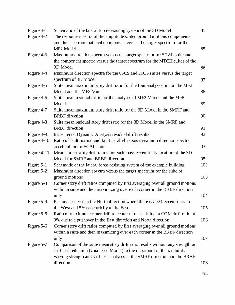
While a structural design should accommodate heavy damage during the maximum considered

earthquake (MCE), the design should also account for less damage as the magnitude of the

earthquake decreases, as deemed necessary by the decision makers and stakeholders. As can be

seen in Figure 2-1, it is possible for several designs of the same building to satisfy the life safety

requirement but have differing performance under lower intensity earthquakes. At the MCE, all

three structural designs shown exhibited extreme damage, but under all other levels of

earthquake occurrence, none of the designs had the same level of damage.

Figure 2-1. Potential behavior of structural designs when subjected to various earthquakes

7

Design 1 behaves poorly under small ground motions, as the damage is high even under frequent

earthquakes. On the other end of the spectrum, Design 3 has very little damage to the structure

for all earthquakes other than the MCE, which could potentially be a costly overdesign. Design 2

may represent an economic design, as it meets life safety requirements for extreme earthquakes,

has moderate damage during rare earthquakes, and minimal damage under frequent earthquakes.

The goal of PBEE is to provide a framework for stakeholders to determine to acceptable levels of

damage and safety for each individual project (FEMA 2006). Both Incremental Dynamic

Analysis and fragility curves are useful tools in the application of Performance Based

Earthquake Engineering. These two related topics will be reviewed in detail within this

Literature Review.

2.2. Incremental Dynamic Analysis

2.2.1. Background

Incremental Dynamic Analysis (IDA) is a method of structural analysis that is used to predict the

behavior of structures under varying levels of dynamic loads. IDA provides a way to determine

the behavior of a structure at multiple limit states to make sure that an economical design is

being provided for a wide range of potential hazard levels, not just the maximum considered

earthquake. IDA is generally performed by incrementally scaling a suite of ground motions to

increasingly higher levels and determining the structural response at each one of these intensity

levels. In IDA, intensity measures (IM) are generally the scale factors applied to the suite of

motions, and damage measures (DM) are the specific responses of the system that is measured

with respect to the different intensity measures. Possibilities for these damage measures include

peak floor accelerations, interstory drifts, and plastic hinge rotations (Vamvatsikos 2002). The

levels of damage are typically shown with the use of an IDA curve, which plots the damage

measure with respect to the intensity measure.

2.2.2 General Procedure of Incremental Dynamic Analysis

IDA relies on scaled ground motions to determine the behavior of the structure at various limit

states. The ground motions used must first be scaled to a common value of spectral acceleration

to remove variability between records. Shome and Cornell (1998) found that scaling to the

design spectral acceleration (using between 5 and 20 percent damping) of the structure’s first

mode period of vibration (or the highest period of vibration) is the best alternative for scaling.

These ground motions are then incrementally scaled to a variety of intensities to relate behavior

and damage to the intensity of the earthquake.

Figure 2-2 shows an example of an IDA plot and the different behaviors that can be typically on

such a plot. In this example, each line on a plot represents the behavior as subjected to one

earthquake record, and 44 different records were used in analysis. Each ground motion record

was systematically scaled up until collapse occurs. At each intensity, the maximum damage

8

measure (which in this case is the drift ratio) is recorded and plotted against the corresponding

scale factor. There are three possible trends that can be seen in the IDA curves. One earthquake

could produce a softening curve (where the slope of the curve decreases between scale factors),

which indicates more damage for increasing increments of intensity, or behavior tending toward

collapse. A different record could result in a hardening curve (where the slope increased between

scale factors), which indicated less damage for increments of intensity. The third trend is a

weaving curve, where the slope increases between some scale factors but decreases between

others.

Figure 2-2. Example IDA curve

IDA curves can be used to predict behavior under a wide range of earthquake intensities, and

therefore, can be used to design and evaluate structures for varying limit states, which is the

principle behind PBEE. For use in PBEE, these physical damages measures are converted into

consequences, which describe the damage in a fiscally quantifiable way. These consequences

(also known as damage variables) could include loss of use, repair costs, potential loss of life,

etc. They can be expressed either as annual probability of occurrence or life cycle probabilities,

depending on the desire of the shareholders (Deierlein et al. 2003).

The process of performing an IDA analysis is focused on determining the behavior of a structure

from its elastic behavior all the way up to failure. The first step in performing the analysis is to

select a suite of ground motion records that could adequately represent the potential hazard of the

site. These ground motions should be sufficient in number to include a wide variety of possible

earthquakes that could occur near the structure and should be carefully determined based on the

soil and fault types that are typical in the vicinity of the structure (Dhakal et al. 2006).

0 0.05 0.1 0.15 0.2 0.250.4

0.6

0.8

1

1.2

1.4

1.6

1.8

2

2.2

2.4

IDA

Scale

Facto

r

Drift

Spaghetti Curve for Drift

Drift Ratio

0 0.05 0.1 0.15 0.2

1.2

2.4

0.6

1.8

IDA Scale

Factor

9

While the example in Figure 2-2 shows the results of Incremental Dynamic Analyses from

multiple ground motions applied to one structure, IDA curves can also be developed for one

ground motion applied to multiple variations of a structure. These “variation of parameter” IDAs

can be useful to determine the potential influence that modeling assumptions or various designs

can have on the behavior of a structure. In this case, the ground motion record used is the

constant, and the mathematic model is the variable that is being altered.

For IDAs to provide the most helpful results, care should be taken to decide which damage

measures and intensity measures would be the most appropriate. For example, for the intensity

measure, the spectral acceleration of the dominant mode would be a good measure, which for

low rise buildings would be the first mode. However, this would not be an accurate assumption

for high rise buildings, as dominant modes could include the higher ones. Each individual

structure will react differently to an earthquake, and selecting a representative intensity measure

is crucial for predicting accurate behavior. Similarly, the damage measure will vary based on

what part of the structure is being analyzed. Peak floor accelerations would be most applicable to

measure the damage to equipment and some non-structural components, while interstory drift

ratios may be the best choice to measure the damage and potential for instability of structural

components (Vamvatsikos and Cornell 2002). The IDA curves are then produced by

interpolating between the measured values of intensity versus damage, and then PBEE can be

applied by defining the desired limit states at specified ground motion intensities and using the

curves to determine how often the chosen limit state is exceeded.

The major limitation of IDA is the heavy computational demand of the analysis. Due to the high

number of analyses that need to be run to produce the IDA curves, this method may not be

reasonable for some applications that require a method with minimal computational requirement.

There is also a significant amount of subjectivity when it comes to determining the appropriate

ground motions, intensity measures and damage measures. Choosing different ground motions

can have significant effects on the results (showing high variability on the response), and

choosing incorrect measures may provide results that do not clearly describe the most critical

behavior of the system (Villaverde 2007).

2.2.3 Applications of Incremental Dynamic Analysis

Despite potential limitations, numerous successful applications of traditional IDA have been

studied and presented. Many examples of these applications came from research performed at

Virginia Polytechnic Institute and State University. Early research was performed on steel

moment frames with viscous fluid dampers that used IDA to investigate the effect of different

types of dampers in the system (Oesterle 2003). This study used 12 earthquakes, half of which

were near fault earthquakes and half of which were far-field earthquakes measured in Los

Angeles, scaled to twenty different intensities. The damage measures included interstory drift

10

ratios, base shears and residual deformations, and the IDA curves were used to determine

behavior changes of different damper types.

The following year, IDA was used at Virginia Tech to investigate the behavior of structures with

hyperelastic braces (Saunders 2004) and to investigate behavior of low-rise buildings in the

Western United States versus the Central and Eastern United States (Spears 2004). The study by

Saunders explored the behavior of hyperelastic elements, which were defined as nonlinear elastic

members that gain stiffness as they are deformed and are beneficial to the structure primarily

near instability. IDA curves were developed using two different scaled earthquakes and two

different P-delta scenarios, using interstory drift and base shear as damage measures. The study

by Spears (2004) investigated whether buildings in Central and Eastern United States were more

susceptible to collapse as associated with vertical accelerations than the structures in the Western

United States. The study used five different locations for each with varying periods and used

IDA to determine the post yield stiffness ratio of each scenario. This research found that

structures in the Central and Eastern United States designed to code were more prone to sudden

collapse that structures designed to code in the Western United States.

Another thesis from Virginia Tech studied the behavior of hybrid steel moment frames, which

considered combinations of ordinary, intermediate and special moment frame connection in the

same structure (Atlayan 2008). For this work, the base intensity measure used was the 5 percent

damped ASCE 7 design spectral acceleration for the period at the first mode of vibration. Ten

sets of ground motion data were used in this research, each of which was scaled to match the

ASCE 7 design spectrum. They were each then scaled 10 more times with scale factors ranging

from 0.2 to 2.0, which means that the structure was analyzed up to two times the ASCE design

strength. For the damage measures, interstory drift, base shear, and maximum and residual roof

displacement were investigated. The focus of the results was determining the potential that the

structure would exceed ASCE 7 drift limits and what the probability of collapse was of the

system under the varying loads. For the hybrid steel systems, the damages measures were

maximum and residual roof displacements, peak base shear, and ductility demand, and the focus

of the analysis was to determine improvements that were given by using a hybrid moment frame

over a traditional one.

An additional hybrid moment frame was investigated at Virginia Tech using IDA, but with this

one focusing on the addition of hybrid passive control devices (Marshall 2008). These hybrid

passive control devices combined two different passive control devices: one that helps dissipate

energy at all deformations (a viscoelastic damper) and one that only engages to dissipate energy

under heavy loading (a buckling restrained brace). To perform IDA on these systems, multiple

earthquakes were scaled 8 times, including a scale factor of 1.0 to represent the design basis

earthquake and another scale factor of 1.5 to represent the maximum considered earthquake.

11

Multiple damage measures were used to determine overall behavior of the systems, including the

maximum roof drifts, base shears and roof accelerations.

Another group of researchers used IDA to investigate the behavior of wood-framed buildings

under seismic loads (Christovasilis et al. 2009). The motivation for this research came from the

significant property loss and loss of life from damage to wood-framed structures in both the 1994

Northridge earthquake and the 1995 Kobe earthquake. Due to the short height of the structures

investigated in this study, the intensity measure used was based on a set of ground motions

scaled to the median spectral acceleration analyzed at a period equal to 0.2 seconds. The set of

ground motions consisted of the 22 bi-directional records used in the FEMA P-695 project

(FEMA 2009a). The prominent mode of failure investigated in this research was global side

sway, which was quantified using a damage measure of peak interstory drift along any wall line.

The probability of collapse was determined by how many ground motions caused the structure to

exceed the predetermined drift limit with respect to how many ground motions were analyzed,

and fragility curves were produced to show the relationship between intensity and probability of

failure.

Further research has also been performed on steel moment frames using IDA to determine the

differences between ordinary, intermediate and special moment frames (Asgarian et al. 2010). In

light of the failure of welded moment frames in the 1994 Northridge earthquake, part of this

research focused on the modeling of the beam column connections, which are especially crucial

during inelastic behavior. OpenSEES (McKenna 2011) was the program used to analyze the

system, including these carefully modeled connections. Three five-story and two ten-story

buildings were used in the analysis, and 15 ground motion records were used for the analysis.

Similar to the works performed by Vamvatsikos (2002) and Atlayan (2008), the damage measure

was chosen to be the maximum interstory drift ratio, and the intensity measure was the 5 percent

damped spectral acceleration associated with the first mode. Once again, IDA proved to be a

beneficial tool for analysis and comparison of systems for more than just life safety limit states.

A similar study (Medina and Krawinkler 2005) investigated the behavior of non-deteriorating

seismic-resisting frames under seismic loads including the influence from P-delta effects. The

height of the buildings varied from three to eighteen stories, and each height was analyzed at two

different periods: 0.1N and 0.2N, where N equals the number of stories. Forty ground motion

records were used, and they all were California earthquakes that were not measured at near fault

locations. Again, drift values, both peak roof and interstory, were the chosen damage measure,

and IDA curves were created for these parameters.

An example of the “variation of parameter” IDA can be found in a study by Dolsek (2009). A

four-story reinforced concrete building was used to examine the effect of these variations

12

including mass between stories, strength of the materials, damping and modeling of the plastic

hinge regions. Fourteen sets of ground motions were used, and multiple models were analyzed to

investigate the effects of these modeling variations, as well as the effects of sample size. The

study determined that a sample size of twenty structures was adequate for this analysis, and that

increasing the sample size beyond that does not significantly change the results. The intensity

measure used was the peak ground acceleration, and the damage measure of maximum drift was

used to quantify the influence of the modeling uncertainties listed previously. The study found

that the extended IDA did not differ much from the traditional IDA in the stages far from

collapse; however, there was a noticeable reduction in collapse capacity for some of the

modeling uncertainties. The uncertainties that had the greatest effect were the ones that

contributed to the failure mechanism, including initial stiffness and rotation in plastic hinge

regions. While this additional aspect of IDA may produce more conservative results for life

safety limit states, the additional computational time and computing power necessary to run such

analysis should be taken into consideration.

IDA has also been used to evaluate the effectiveness of current and past codes to design seismic

resisting systems. There have been numerous studies where both new and existing structures

were investigated in high and low seismic area in the United States. In one example, several

reinforced concrete structures conforming to different code editions with varying seismic-

resisting systems were analyzed using IDA (Liel et al. 2006). Using 22 sets of ground motion

with two components each, curves were plotted to predict the probability of collapse with respect

to the ground motion acceleration. While the research showed that current codes provide better

resistance to seismic loads than previous codes, it found that there was still work to be done to

account for variability in the design and loading of seismic-resistant systems.

Similar analyses have been performed for steel moment frames with a focus on the differences in

code provisions before and after the 1994 Northridge earthquake (Yun et al. 2002). As a result of

this earthquake, there were noticeable problems with the design of moment frames, which

spurred a revamping of the code requirements of these systems. IDA using 20 ground motions

and a damage measure of interstory drifts found nearly identical results to the study on

reinforced concrete resisting systems by Liel et al. (2006). Both studies determined that systems

designed to newer codes have a much lower probability of collapse, but that variability in

loading and behavior provide a difficulty in dynamic analysis.

Another interesting example of the use of IDA has been to use the procedure to quantify the

residual capacity in a structure after the earthquake and determine the probability of collapse due

to an aftershock (Luco et al. 2004). While all the other examples have investigated the behavior

of initially undamaged structures that are subjected to earthquakes for the first time, this study

takes it one step further to determine the likely behavior of buildings that were damaged during a

13

previous earthquake, and then subjected to an aftershock. After an earthquake occurs, many

standing structures will not be safe to occupy and will need to be kept vacant. To realistically

determine if this is a necessity, nonlinear dynamic analysis should be performed, but in the

critical time after an earthquake, this would often not be a possibility. This study presents a case

study that analyzes the structure both during the earthquake and during an aftershock to

determine the residual capacity the building could have using IDA. Performing an analysis of

this nature before an earthquake even occurs could provide valuable information about the

probable condition of the building, which would then be available immediately after the

earthquake. Accuracy in determining residual capacity is critical to understanding both potential

life safety and down-time losses of the structure after the event. In the case study, IDA curves

were provided for the peak displacement for sequences of accelerations from main shocks

followed by aftershocks.

While the vast majority of examples of IDA have been performed in two dimensions (2D), the

process can be expanded to three dimensions (3D). Analyzing a structure in 3D is necessary for

structures that are not symmetric and require the scaling of two components of ground motion.

Analysis using two ground motions together to determine response is the major difference in 3D

analysis, an example of which was investigated for a 20-story steel space frame (Vamvatsikos

2006). Another example of this application of 3D IDA analysis was a circular prestressed bridge

(Vamvatsikos and Sigalas 2005). Special care was taken when selecting the intensity measures

and damage measures to ensure that the analysis would accurately represent the structural

response in both directions, as different parameters would control the maximum response in each

direction and the governing case needs to be predicted. Twenty-two ground motions were used,

and they were applied to system using the two orthogonal ground components applied

simultaneously.

Incremental Dynamic Analysis has become increasingly popular due to its use in the FEMA P-

695 Methodology (FEMA 2009a). This methodology was been developed to “provide a rational

basis for establishing global seismic performance factors, including the response modification

coefficient (R), the system over-strength factor (0), and the deflection amplification factor (Cd)

of new seismic-force-resisting systems proposed for inclusion in model building codes” (FEMA

2009a). In this procedure, Incremental Dynamic Analysis is performed using a suite of 44 or 56

ground motions components that are incrementally scaled until structural collapse occurs. This

methodology has become widely used in the earthquake engineering research community, and

numerous examples of this procedure can be found, many of which are compiled in the ATC-76

report (NIST 2010a). As an example, Figure 2-2 shows the IDA results of the FEMA P-695

procedure applied to a seven-story steel moment frame that included the modeling of the lateral

resistance of the gravity system (Flores et al. 2012).

14

2.2.4. Alternative Methods to Incremental Dynamic Analyses

2.2.4.1. Comparison to Nonlinear Static Pushover Analysis

Simplified methods, including nonlinear pushover analysis, have been used as an alternative to

Incremental Dynamic Analysis, as they provide a method that is considerably less

computationally demanding. However, IDA provides significantly more insight into the inelastic

behavior of a structure, particularly its behavior near collapse. The major limitation of this

simplified method is that static pushover analyses do not usually take into account the change in

modal properties that occurs when a structure is deformed inelastically under seismic loads.

When comparing the results of IDA and pushover analysis, it has been shown that they

correspond well in the linear range of the structural behavior, although, after yield, the two

methodologies produce different results. While static pushover analysis can provide accurate

results for the sequencing of yielding or failure in more ductile systems, this method does not

include higher modes and can easily become inaccurate during inelastic behavior (Antoniou and

Pinho 2004). The static pushover method determines the “capacity” of a given structure, but does

not inherently consider the “demand” of a potential seismic event. Because both are needed to

accurately design a structure, dynamic analysis does seem to be a necessary computational tool

(Elnashai 2002).

IDA provides an alternative method to the traditional static pushover analysis that does not have

the same shortcomings regarding the inelastic range and higher modes. The results from the IDA

will generally follow an extrapolation of the static pushover results using the equal displacement

concept up until hardening occurs. Work has been done (Vamvatsikos 2002) to produce IDA

type curves using static pushover analysis, which simplifies the analysis. While the concept of

IDA provides more accurate, in-depth results, it was shown that the static pushover test can

create approximate curves with significantly less computational need.

This idea that pushover tests can be sufficient in analysis of structures under seismic events was

further investigated (Han and Chopra 2006). The study by Vamvatsikos (2002) only investigated

a nine-story steel moment frame system, but this newer research used three buildings varying in

height that included a three-story, nine-story and twenty-story building. Results were similar to

that of the Vamvatsikos study and stated that a modal pushover analysis (MPA) could be an

appropriate simplified method of analysis to create fragility curves without the use of response

history analysis. According to the results of this study, the accuracy did not vary between the

buildings of varying height, although the dynamic analysis became more involved, and the

pushover method of analysis produced accurate behavior even up through instability and collapse

as long as a proper hysteretic model was chosen to represent the modal behavior.

Another study comparing IDA to pushover analysis investigated reinforced concrete structures

(Mwafy and Elnashai 2001). Twelve reinforced concrete frames of varying height and structural

15

system were used in the analysis. This research found that the two methods have similar results

in the elastic regions, and although they often vary after yield, the pushover method provides a

conservative analysis, when compare to the Incremental Dynamic Analyses. This study also

concludes that pushover analysis appears to be a good approximation for IDA results,

particularly in the elastic region (even though the elastic range rarely provides the information

desired from an IDA), and could be an applicable alternative, especially in a real-world design

scenario where simplicity in analysis is highly preferred.

However, research has been performed that disagrees with this conclusion. In a literature review

(Villaverde 2007) discussing multiple methods to analyze collapse of buildings, numerous

studies were found that analyzed the steel moment frames designed prior to the 1994 Northridge

earthquake with both static pushover and non-linear dynamic analyses, like IDA. In these

studies, the results of the methods differed greatly, and they found that the pushover tests

actually calculated drifts that were un-conservative and predicted the incorrect locations of

yielding regions. This same literature review states that these problems can arise in a pushover

test because “it neglects duration and cyclic effects, the progressive changes in the dynamic

properties that take place in a structure as it experiences yielding and unloading during an

earthquake, the fact that nonlinear structural behavior is load-path dependent, and the fact that

the deformation demands depend on ground motion characteristics.”

2.2.4.2. Additional Alternative Methods of Incremental Dynamic Analysis

Other methods have been introduced that provide alternatives to IDA. One such method that has

been presented is the Endurance Time Method (Estekanchi et al. 2004). The basis of this method

is determining how long a structure can remain stable under certain dynamic loading; in other

word, what is the structure’s endurance? Accelerations are applied to the structure in a ramp type

loading, so the method determines how long the structure will be able to withstand this

increasing loading. The longer the structure stays standing, the better the performance.

Endurance limit points are specified to desired levels of performance, and the endurance time is

the length of time it takes to reach the specified limit points. Similar to IDA, these limit points

will be based on physical behavior like drift and accelerations in the structure and need to be

chosen based on relevance to the structure that is being investigated. Like any method of

dynamic analysis, determining appropriate dynamic simulation and performance of the collapse

analysis can prove to be a hindrance in this type of method.

Another method that has been presented as an alternative to IDA is probabilistic seismic demand

analysis (Mackie and Stojadinovic 2002). As opposed to IDA, which selects a set of earthquakes

and scales them to different intensities, the probabilistic seismic demand analysis (PSDA) uses a

large set of earthquake data that inherently incorporates a range of intensities. The main

difference in the two methods is that PSDA uses the “bin strategy,” which uses a large number of

16

earthquake records in analysis and subdivides them according to magnitude, distance and soil

type. IDA, on the other hand, relies on a small number of records that are scaled multiple times

to imitate other potential earthquake records. In the Mackie and Stojadinovic study, both the IDA

and the PSDA are run 80 times; the PSDA did so using four bins of 20 earthquakes, while the

IDA used four ground motions scaled 20 times. If behavior with respect to intensity is not the

only concern, PSDA can be a more informative method, as it also provides information response

at different distances and on different soil types. However, this study shows that with careful

selection of the earthquake records for IDA, the two methods can be used interchangeably. The

same information can be determined in IDA, but the smaller batch of earthquakes chosen must

have necessary variation.

One last method that will be discussed in this paper is a method that combines pushover analysis

with aspects of Incremental Dynamic Analysis to provide a more computationally efficient

method (Liel and Tuwair 2010). In this method, an initial nonlinear static pushover test is

performed to find an initial estimation of median spectral acceleration of the collapse resistance

of the structure, and numerous methods are proposed to estimate this parameter from a pushover

analysis. The suite of ground motions selected to analyze the building are then scaled to this

acceleration, and analysis is run. If this spectral acceleration does not equal the median

acceleration (half of the analyses result in collapse), the acceleration is iterated and the analysis

repeated until it does reach the median acceleration.

An advantage of the Leil and Tuwair method is the reduction in the number of ground motions

required for subsequent analysis. Once a ground motion is known to cause a collapse at a certain

intensity, it is assumed that it would cause collapse under stronger ground motions and can be

eliminated in iterations if the initial median acceleration value was found to be too small. The

opposite holds true if the initial value should be decreased; ground motions that did not cause

collapse can be ignored for weaker ground motions. The computation saved by having an initial

estimate from pushover analysis and reducing ground motions used in subsequent runs decreases

run times by approximately 90 percent and provides answers within 8 percent of the answers

from Incremental Dynamic Analysis of the same structures.

2.3. Fragility Curves

2.3.1. Introduction to Fragility Curves

Fragility curves provide a method to summarize the results of numerous dynamic analyses (like

IDA) from a probabilistic perspective. A fragility curve, in the most simple terms, is a statistical

distribution that can describe the probability of any occurrence, whether that occurrence is

collapse or minor structural damage or something in between. Fragility curves are developed by

defining an engineering demand parameter (EDP) and a damage measure (DM), which are

recorded during numerous dynamic analyses. The fragility curve provides the probability of

17

exceeding a certain damage limit state, given as a value of the DM, with respect to the EDP

(Porter et al. 2007).

2.3.2. Relationship between IDA and Fragility Curves

Incremental Dynamic Analysis is a popular tool used for dynamic assessment of structures and

the application of Performance Based Earthquake Engineering, and it is more prevalently used

than any of the alternative methods. However, IDA provides an extensive set of structural

response results, which needs to be summarized to be practical for engineers and researchers.

Fragility curves provide a method to summarize these results from a probabilistic perspective. As

mentioned previously, fragility curves show the probability of exceeding any limit state, which is

typically defined by a damage measure or intensity measure recorded during the Incremental

Dynamic Analyses. The development and application of fragility curves is discussed in the

remainder of this section, including the procedure to develop fragility curves from IDA results.

In order to begin the discussion on fragility curves, however, review of basic statistics is needed,

which is provided in the next section.

2.3.3. Background on Necessary Statistics

To develop the necessary statistical tools, two textbooks were consulted (Ang and Tang 2007,

Ott and Longnecker 2010), and all the equations and discussion for the remainder of this section

were from these sources.

2.3.3.1. Mean and Standard Deviation

The first step in statistics that is necessary to develop fragility curves is to define the mean and

standard deviation of a set of data with n number of data points, with the data points represented

as xn. This data set could be anything of interest to the user. For example, the data set could

define the lateral deformations in racking tests of drywall that correlate with the first

observations of cracking, or it could contain the acceleration values where each individual

ground motion caused collapse of a structure during a P-695 analysis. Any set of results can be

summarized in a fragility curve by finding some key statistical properties, including the mean

and standard deviation. The mean, µ, is the average of the data, and the standard deviation of the

population, σ, is a measure of the variability or spread of the entire data set. The equations for

these two variables are shown below in Equation 2-1 and Equation 2-2, respectively.

∑ (2-1)

∑ (2-2)

18

These two parameters become the basis for developing the distributions that will be discussed

later in this section.

2.3.3.2. Probability Density Functions and Cumulative Distribution Functions

A probability density function (PDF) represents the frequency of occurrence of a value in a set of

random variables. The total area under a PDF is always equal to 1.0, and the probability that a

random variable is between two values is the integral under the PDF between those two values,

as shown in Equation 2-3. By integrating under the entire area of a PDF, a cumulative

distribution function (CDF) is developed, which shows the probability of occurrence of a random

variable. These curves approach zero for -∞ and 1 for +∞, and the probability of occurrence that

a random variable is less than or equal to a value of interest is shown below in Equation 2-4.

∫

(2-3)

∫

(2-4)

where: fx(x) is the equation of the PDF

Fx(x) is the value of the CDF

X is the random variable

x is the value of interest

Figure 2-3 shows an example of a PDF (left) and its corresponding CDF (right) for a set of

normally distributed randomly generated variables between 1 and 100.

Figure 2-3. A probability density function (left) and its corresponding cumulative distribution

function (right) of a set of randomly generated numbers

0

0.002

0.004

0.006

0.008

0.01

0.012

0.014

0.016

0 50 100

fx(x

)

x

0

0.1

0.2

0.3

0.4

0.5

0.6

0.7

0.8

0.9

1

0 50 100

Fx(x

)

x

19

The CDF shows the typical shape of a fragility curve, where for any value of x, the probability of

occurrence, Fx(x), can be determined. Traditionally in fragility curves, x will represent the range

of the engineering demand parameter, and the CDF will give the probability of occurrence for a

value of a limiting damage measure. In order to solve for the CDF, a PDF needs be defined. To

do so, one of the numerous statistical distributions can be fit to the set of data. Two of the more

popular distributions, normal and lognormal, are discussed next.

2.3.3.3. Normal distributions

One potential distribution that can be applied to data is the normal distribution. This distribution

assumes x values can be between -∞ and +∞, and the PDF is defined next in Equation 2-5.

√

[

(

) ] (2-5)

where: N( ) is the normal distribution

2.3.3.4. Lognormal distributions

Another potential distribution is the log-normal distribution. This distribution differs from the

normal distribution in that it assumes that x values can be between 0 and +∞, which makes it a

good distribution for data sets consisting only of positive numbers. The PDF for this distribution

is defined in Equation 2-6.

√

[

(

) ] (2-6)

where: N(λ,) is the lognormal distribution

λ is the mean of ln(x), the natural log of the data set

is the standard deviation of ln(x)

2.3.3.5. Defining distributions in software

PDFs and CDFs for distributions are easy to build in software programs given a set a data values,

and this section is included to give the Microsoft Excel (Microsoft 2010), Mathcad (PTC 2012)

and Matlab (Mathworks 2011) commands used to build these functions. This section will focus

on the commands to build normal and lognormal distributions, but it is important to note that

many other distributions are available in these programs, even though they are not discussed

here. The data points should be sorted from smallest to largest value, and then the mean and

standard deviation need to be determined for the set of data. The command to find the mean,

standard deviation, PDF and CDF for each program is shown in Table 2-1.

20

Table 2-1. Statistical commands in common software programs

Excel Mathcad Matlab

Mean, µ = average(X) = mean(X) = mean(X)

Std. deviation, σ = stdev(X) = stdev(X) = std(X)

Normal PDF = NORM.DIST(x,µ,σ,false) = dnorm(x,µ,σ) = normpdf(x,µ,σ)

Normal CDF = NORM.DIST(x,µ,σ,true) = pnorm(x,µ,σ) = normcdf(x,µ,σ)

Lognormal PDF N/A = dlnorm(x,µ,σ) = lognpdf(x,µ,σ)

Lognormal CDF = LOGNORM.DIST(x,µ,σ) = plnorm(x,µ,σ) = logncdf(x,µ,σ)

where: X is the full set of data points in vector form

x is each individual data point

In Excel, the commands are simply typed in the cells, while in Matlab and Mathcad, the

commands must be assigned to a variable.

2.3.4. Building Fragility Curves

When a large set of results has been collected, it is important to summarize the results, which can

be done using fragility curves. From the perspective of earthquake engineering, these results can

come from Incremental Dynamic Analyses, lab tests, or any other method of producing a set of

data that describes behavior under dynamic loading. Initially, a measure of the limit state will

need to be determined to begin the process of developing a fragility curve. Again, this limit state

could be the first observations of cracking in drywall defined by the lateral displacement, or

structural collapse defined by the acceleration level, or any other behavior of interest. Once the

measure is chosen, it is crucial to note whether it is a numerical measure or an event, because this

will determine how the curve is constructed.

If the damage measure is a numerical value, like interstory drift, the fragility curve can be

developed using a statistical distribution. For structural response, a lognormal distribution is

typically used because the peak absolute value of drift is always positive. For the chosen

probability distribution (normal or lognormal), the appropriate mean and standard deviation of

the data should be found and used to build the CDF of that distribution. This CDF is the fragility

curve that will provide the probability of occurrence of a damage state (e.g. first cracking of

drywall) for the range of the numerical damage measure (e.g. interstory drift).

If the damage measure is an event, for example collapse, a different approach is needed to

develop the distribution. Instead of using a distribution function, a count will be necessary to

build the fragility curve. At each ground motion intensity the number of earthquakes that cause

the collapse event to occur will need to be counted. The probability of this event for one intensity

of motion will equal the number of occurrences at that intensity divided by the total number of

21

earthquakes analyzed. This process will be repeated for each intensity, and the fragility curve

will plot the probabilities of occurrence with respect to the intensity used in analysis.

2.3.5. Application to FEMA P-695

For this methodology, a collapse fragility curve is built as a cumulative distribution function of a

lognormal distribution using the median collapse intensity ( SCT ) and a standard deviation value

called the record-to-record dispersion (RTR). The median collapse spectral acceleration is found

during the Incremental Dynamic Analyses as the intensity at which 50 percent of the analyses

have caused structural collapsed. Typically, RTR is equal to 0.4, but can be as low as 0.2 for

systems with low ductility. The calculation of this value is shown in Equation 7.2 of FEMA P-

695 (FEMA 2009a). It is important to note that this differs from traditional lognormal

distributions where the mean of the natural log of the data is usually used instead of the natural

log of a median value.

The procedure for developing a collapse fragility from a set of P-695 Incremental Dynamic

Analyses will be shown for the same example presented in Figure 2-2. Again, these results are

for a seven-story steel moment frame that included the modeling of the lateral resistance of the

gravity system (Flores et al. 2012). The IDA results are shown again in Figure 2-4, but with

additional information. In the FEMA P-695 procedure, the collapse margin ratio (CMR) is

defined as the scale factor on the spectral acceleration of the maximum considered earthquake

(MCE) at the fundamental period of the structure where half of the ground motions have caused

the structure to collapse. In other words, the CMR is the ratio of median collapse intensity ( SCT )

to the MCE intensity (SMT).

Figure 2-4. Example IDA curve with Collapse Margin Ratio shown

0 0.05 0.1 0.15 0.2 0.250.4

0.6

0.8

1

1.2

1.4

1.6

1.8

2

2.2

2.4

IDA

Scale

Facto

r

Drift

Spaghetti Curve for Drift

Drift Ratio

CMR = 2.2

0 0.05 0.1 0.15 0.2

1.2

2.4

0.6

1.8

IDA Scale

Factor

22

For this example, half of the ground motions had caused the structure to collapse by a scale

factor of 2.2, which defines the CMR for this structure. This structure had a MCE intensity of

0.5625g, and therefore, the median collapse intensity is 1.2375g. The collapse fragility, shown in

Figure 2-5, is then developed using a lognormal distribution defined by the natural log of the

median collapse intensity and a record-to-record dispersion of 0.4.

Figure 2-5. Example collapse fragility curve

2.3.6. Other Examples of Previous Fragility Analysis

FEMA P-695 type applications are not the sole use for fragility curves in structural engineering.

Numerous other research projects have discussed the use and development of fragility curves,

many of which will be discussed in this section.

One study investigated the influence of the number of stories on the behavior of an ordinary

concrete building (Akkar et al. 2005). This paper found the capacity of typical concrete buildings

in Turkey using real data from 32 buildings and subjected them to a suite of 82 ground motions.

Peak ground velocity was chosen as the engineering demand parameter, as it was believed to be

a better representation of the inelastic behavior, and a displacement-based limit state of global

drift was chosen as the damage measure. Fragility curves were made for each building height to

plot the probability of exceeding a limit for the chosen limit values of light, moderate and severe

drift with respect to the peak ground velocity.

Another study on concrete behavior investigated slab column connections of 82 specimens and

used interstory drift and vertical shear ratio limits to define four limit states: light cracking,

heavy cracking, punching shear failure, and loss of vertical carrying capacity (Aslani and

Miranda 2005). In that study, the fragility functions were developed using a log-normal

0

0.1

0.2

0.3

0.4

0.5

0.6

0.7

0.8

0.9

1

0 0.5 1 1.5 2 2.5 3 3.5 4

Pro

bab

ility

of

no

n-e

xce

edan

ce

SA (g)

SCT= 1.24g

23

distribution of probability of exceedance versus the interstory drift or vertical shear ratio.

Concrete moment frames have also been investigated using fragility analysis (Lowes and Li

2010). Seven different moment frames were investigated, and damage levels for three damage

states (cracking, spalling and crushing) were correlated to story drift via fragility curves.

These previous three papers showed examples of how fragility curves can be developed when the

damage measure was a numerical value. An example of developing fragility curves for an event

can be seen in a study on the collapse of structures using varying hysteretic models (Ayoub et al.

2004). Three degradation models were investigated: a bilinear model, a modified Clough model,

and a pinching model. The number of analyses that produced a collapse was divided by the total

number of analyses to determine the probability of occurrence.

Another system that has been studied was a frame with passive controllers (Cundumi and Laboy

2010). This research investigated 30 concrete frames, some high rise and some low rise buildings

that had been augmented with varying additional dampers placed in a variety of configurations,

including a diagonal, chevron, lower toggle or upper toggle. This was also an example where the

occurrence of an event was used to calculate the fragility. If the structure passed a limit state, a 1

was assigned, otherwise a 0 was assigned to indicate that it had not reached the limit state. The

fragility curves for slight, moderate, extensive and complete damage were plotted against the

peak ground acceleration by dividing the sum of the assigned numbers by the total analyses.

While Incremental Dynamic Analysis using multiple response history analyses (RHA) is

typically used in FEMA P-695 type projects to build fragility curves, alternative methods have

been presented. One method used a modal pushover analysis (MPA) that analyzed the structure

only once (Han et al. 2010). Two steel moment frames were analyzed using both RHA and MPA

to compare the differences in collapse fragilities of structures. This study found that MPA

combined with an empirical relationship of collapse strength ratios provided good approximate

results.

While FEMA P-695 provides a suite of ground motions for analysis, alternatives can be used to

develop the suite of ground motions. One popular alternative is Monte Carlo simulation, which

predicts the behavior through random number generation applied to a given probability density

function. One such example was applied to a four-story ordinary reinforced concrete moment

frame (Korkmaz 2008), which compared the results with a more traditional nonlinear dynamic

analysis. This study found comparable results between the Monte Carlo simulation and the

traditional response history analysis, although it recommended that more structures and ground

motions would be necessary to make a valid comparison between the two.

24

A relatively new methodology, FEMA P-58 (FEMA 2012), utilizes fragility curves extensively.

This procedure uses collapse fragilities, like those developed for FEMA P-695, as well as

component fragilities. One of the major goals of this method is to provide results that are

meaningful to owners and decision makers (consequences like costs, repairs and casualties). In

order to convert structural response to these consequences, the component fragilities are used to

show the probability of exceeding discrete damage states with respect to structural response

parameters, like drift or acceleration. These discrete limit states have an associated set of

consequences, and through the use of a few nonlinear response history analyses and Monte Carlo

simulation, the P-58 procedure provides a potential distribution of consequences for any given

ground motion or hazard. The fragility curves play a crucial part in connecting structural

response to the more meaningful consequences.

Further works have used fragility curves to analyze suspended ceilings (Badillo-Almaraz et al.

2007), light frame wood construction (Ellingwood et al. 2004), wood shearwalls (Kim and

Rosowsky 2005), rocking connections (Cimellaro and Roh 2010), and concrete bridges (Karim

and Yamazaki 2003, MacKie and Stojadinovic 2007, Moschonas et al. 2009, Saxena et al. 2000).

Fragility curves have also been developed to investigate the effects of ground motion duration

(Iervolino et al. 2006) and soil-structure interaction due to liquefaction (Koutsourelakis et al.

2002). These studies are mentioned to provide additional resources regarding the uses of fragility

curves, but will not be discussed in more detail, because they are of less relevance to this

research than previously discussed examples and do not provide any additional, unique

information regarding the development and use of these curves.

With any fragility curve, there is uncertainty that can be accounted for. Initially, there are

uncertainties involved with the chosen distribution, and a measure of the goodness of fit should

be performed. Examples and applications of this have been discussed, including in studies on

slab column connections and on bridge damage from the 1995 Kobe earthquake (Aslani and

Miranda 2005, Shinozuka et al. 2000). There is also uncertainty involved in the behavior of the

structure in analysis. Two types of these uncertainties are discussed in Zareian and Krawinkler

(2007). Aleatory uncertainties come from natural randomness, which in this study was from

record-to-record variation of the ground motion. Epistemic uncertainty, on the other hand, comes

from inaccurate representation of the structure and the idealization of the model. Both can cause

large variations in results, and the Zareian and Krawinkler study provides a method to find the

effects of these uncertainties by determining the confidence of the fragility curve and adjusting

the curves to account for highly spread confidences.

Studies have also been performed to identify which damage measures and engineering demand

parameters are best to use to determine the inelastic behavior of structures. One such study

investigated structures with energy-dissipating devices and found the behavior with damage

25

measures of story drifts, maximum column moments and axial force in bracings analyzed with

respect to engineering demand parameters of peak ground acceleration, peak ground velocity,

spectral pseudo velocity and spectral pseudo acceleration (Dimova and Elenas 2002). This paper

provided a general procedure to determine which parameters provide the most accurate and

insightful results, and examples of this procedure were given for four structural systems analyzed

with combinations of the damages measures and demand parameters listed above.

2.3.7. Goodness of Fit Tests

If a statistical distribution is fit to the data, a goodness of fit test is needed to determine how

accurate the assumed distribution fits that data. There are numerous goodness of fit tests

available, three of which will be discussed in this section.

2.3.7.1. Chi Square Test

The Chi Squared test is a goodness of fit test for a PDF where the observed frequency, ni, for a

given interval is compared against the theoretical frequency, ei, where i ranges from 1 to the

number of intervals, k (Ang and Tang 2007). The assumed distribution is acceptable at the

analyzed significance level if:

∑

(2-7)

where: c1-,f is the value of the 2 distribution

is the significance level

f is the degree of freedom = k-1

The assumptions for this test are that k must be greater than or equal to 5, and the values of ei

must also be greater than 5. Since the method is used for PDFs, this one is not applicable to

typical fragility curves, which are CDFs.

2.3.7.2. Kolmogorov-Smirov (K-S) Test

The K-S test is a goodness of fit test to compare test data with the CDF of the desired

distribution. To test the fit, a stepwise distribution, Sn(x), is developed as follows:

Sn(x) = 0 x x1

=

xk x xk+1 (2-8)

= 1 x ≥ xn

where: xk are the values of the data set listed from low to high

n is the sample size

26

The maximum difference between this function and the CDF of the assumed distribution, Fx(x),

is determined using Equation 2-9. The upper limit is calculated as Dn, which is tabulated in

Table A.5 of Ang and Tang (2007) and is dependent on .

| | (2-9)

The assumed distribution is acceptable at the analyzed significance level if:

(2-10)

2.3.7.3. The Anderson-Darling (A-D) Test

As opposed to the K-S test, the A-D test puts more weight on the tails of the distribution, which

can be helpful to determine the influence of outliers. The data is listed from low to high, where i

ranges from 1 to n, with n being the sample size. The CDF is then evaluated at each data point

using the desired distribution, Fx(xi). The A-D statistic, A2, is determined as shown in Equation

2-11, and the adjusted A-D, A*, statistics is calculated as shown in Equation 2-12.

∑ [ { }

]

(2-11)

(

) (2-12)

The next step is to calculate the critical value, c, which depends on the desired distribution. For

the normal and lognormal distributions, c is determined as:

(

) (2-13)

where: a, b0, b1 are tabulated values (Ang and Tang 2007)

The assumed distribution is acceptable at the analyzed significance level if:

(2-14)

The assumption for this test is that the sample size, n, is larger than 7. Like the other two tests,

the result also depends on the significance level, making all three tests subjective.

27

2.3.7.4. An example of the K-S and A-D test

Since these two tests check the validity of the CDFs of a chosen distribution, they will both be

used to determine the acceptability of fitting a normal distribution to the data used for the

standard fragility curve in the previous section. Using a significance level of 0.05, the critical

values for both tests are determined and shown in Table 2-2 for the K-S test and Table 2-3 for

the A-D test. For the A-D test, a, b0 and b1 were calculated as 0.7514, -0.795 and -0.89,

respectively.

Table 2-2. Results for K-S Test

x Sn(x) Fx(x) Dx 1 0.000 0.000 0.000

2 0.143 0.029 0.114

3 0.214 0.331 0.117

4 0.286 0.517 0.231

5 0.357 0.526 0.169

6 0.429 0.527 0.098

7 0.500 0.530 0.030

8 0.571 0.562 0.009

9 0.643 0.602 0.041

10 0.714 0.634 0.080

11 0.786 0.653 0.133

12 0.857 0.698 0.160

13 0.929 0.735 0.194

Dn = max (Dx) = 0.231

14 1.000 0.972 0.028

Dn = 0.29

Table 2-3. Results from the A-D test

i Fx(x) A2

i 1 0.029 0.546

2 0.331 0.562

3 0.517 0.714

4 0.526 0.916

5 0.527 1.141

6 0.530 1.317

7 0.562 1.402

8 0.602 1.456

9 0.634 1.573

10 0.653 1.714

11 0.698 1.758

12 0.735 1.256

A

2 = 1.466

13 0.972 0.112

A* = 1.570

sum = 14.466

c = 0.701

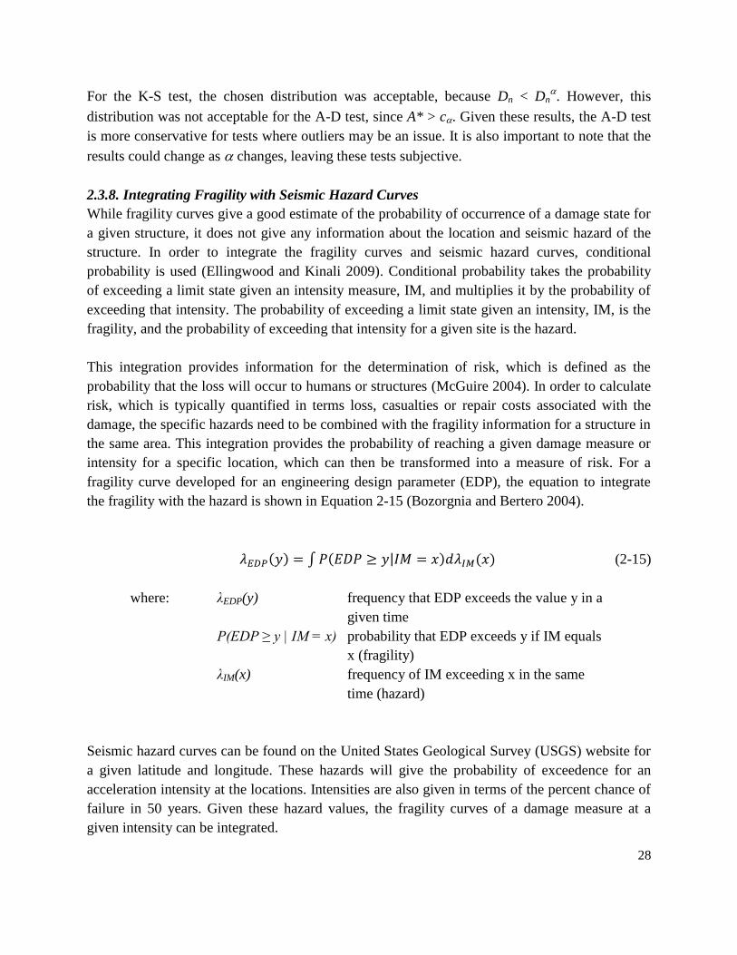
28

For the K-S test, the chosen distribution was acceptable, because Dn < Dn. However, this

distribution was not acceptable for the A-D test, since A* > c. Given these results, the A-D test

is more conservative for tests where outliers may be an issue. It is also important to note that the

results could change as changes, leaving these tests subjective.

2.3.8. Integrating Fragility with Seismic Hazard Curves

While fragility curves give a good estimate of the probability of occurrence of a damage state for

a given structure, it does not give any information about the location and seismic hazard of the

structure. In order to integrate the fragility curves and seismic hazard curves, conditional

probability is used (Ellingwood and Kinali 2009). Conditional probability takes the probability

of exceeding a limit state given an intensity measure, IM, and multiplies it by the probability of

exceeding that intensity. The probability of exceeding a limit state given an intensity, IM, is the

fragility, and the probability of exceeding that intensity for a given site is the hazard.

This integration provides information for the determination of risk, which is defined as the

probability that the loss will occur to humans or structures (McGuire 2004). In order to calculate

risk, which is typically quantified in terms loss, casualties or repair costs associated with the

damage, the specific hazards need to be combined with the fragility information for a structure in

the same area. This integration provides the probability of reaching a given damage measure or

intensity for a specific location, which can then be transformed into a measure of risk. For a

fragility curve developed for an engineering design parameter (EDP), the equation to integrate

the fragility with the hazard is shown in Equation 2-15 (Bozorgnia and Bertero 2004).

∫ | (2-15)

where: λEDP(y) frequency that EDP exceeds the value y in a

given time

P(EDP ≥ y | IM = x) probability that EDP exceeds y if IM equals

x (fragility)

λIM(x) frequency of IM exceeding x in the same

time (hazard)

Seismic hazard curves can be found on the United States Geological Survey (USGS) website for

a given latitude and longitude. These hazards will give the probability of exceedence for an

acceleration intensity at the locations. Intensities are also given in terms of the percent chance of

failure in 50 years. Given these hazard values, the fragility curves of a damage measure at a

given intensity can be integrated.

29

2.4. Background on ASCE 7 Nonlinear Dynamic Analysis Procedure

2.4.1. Methodology

Chapter 16 of ASCE 7-10 (ASCE 2010), which is currently the most recent version of ASCE7

Standard Minimum Design Loads for Buildings and Other Structures, describes the process for

response history analysis. It provides an option for linear response history analysis; however, this

is not of interest to this research and will not be discussed. The nonlinear response history

analysis requires that a model be created to capture all nonlinear behavior of the structure. The

modeling requirements state that the hysteretic behavior must account for any yielding, strength

and stiffness degradation and pinching. The strength of the elements must be the expected

strength and should consider over-strength, strain hardening and degradation. The model should

include a fixed base or appropriate soil-structure interaction. Two-dimensional modeling is only

permitted for systems with independent, orthogonal resisting systems.

This mathematical model is then analyzed with 3 to 7 ground motions scaled to the design

spectrum for the design base earthquake (DBE). The design spectrum assumes an intensity-based

assessment, which means the analysis is performed for one level of potential intensity, which is

the DBE in this case. These ground motions should match in magnitude, fault distance and

source mechanisms of the maximum considered earthquake (MCE), and simulated ground

motions can be used. The building must be analyzed with these ground motions, as well as the

dead load and at least 25 percent of the live load.

This scaling process requires that a SRSS spectrum is created for the 5 percent damped response

spectrum of the components of the ground motion pairs. The average of all the SRSS spectra

must not be less than the design response spectrum between 0.2*T and 1.5*T, where T is the

fundamental period of the structure. If the site is within three miles of an active fault, the average

of the fault normal component spectra should not be less than the design spectrum for the same

range.

If at least seven ground motions are used in the analysis, the design values for the member

forces, inelastic deformations and story drifts can be taken as the average of the results from the

ground motions. If less than seven ground motions are used, the design values must be taken as

the maximum values from the analyses. The member deformations must be less than two-thirds

of the value that causes loss of load carrying capability, and story drift must be less than 125

percent of the story drift limit, which are defined in section 12.12.1 of ASCE 7-10.

2.4.2. Current Implementation

ASCE7-10 has been adopted as the document used in the 2012 International Building Code

(IBC) and the 2012 International Residential Code (IRC) for their structural provisions. A

30

change in philosophy has occurred since the release of this methodology, which has prompted

the proposed changes to the ASCE 7, which are discussed in the next section.

2.4.3. BSSC Proposed Updates

The Building Seismic Safety Council Response History Analysis Issue Team (BSSC RHA IT)

has proposed changes for the next update of ASCE 7 (Haselton et al. anticipated). These

proposed changes will be the focus of the ASCE 7 section of this research. Initially, the ground

motion level has been proposed to be the maximum considered earthquake, instead of the design-

based earthquake. Two options will be proposed for the design spectrum: the traditional code-

based spectrum or one or more scenario-based spectrum.

A suite of eleven ground motions is proposed for the minimum number of records, and vertical

components would now be allowed for analysis. The chosen ground motions should have a

spectrum that closely matches the design spectrum, and simulated ground motions would be

acceptable to fill any gaps in ground motion data. Spectral matched ground motions would be

accepted with an implicit penalty from the scaling procedure. The BSSC also proposes the

requirements that ground motions for near fault sites should include near site effects, including

fault rupture directionality and velocity pulses, when necessary.

For the scaling of the three-dimensional ground motions, the task force proposes that the

maximum direction component of the ground motion records be used, instead of the square root

of the sum of the squares (SRSS). The average of these maximum direction spectra must match

the design spectra as closely as possible and can never be less than 90 percent of the design

spectrum between the period range of interest. For spectrum matched ground motions, single

components would be used, and the average spectra of these components must never be less than

the design spectrum between the period range of interest.

Modeling requirements stay similar, although a few additions are proposed. Elements that are

shown to stay linear can be modeled as linear elements (force controlled elements), effective

additional model damping or viscous damping must not exceed 3 percent, and buildings with

foundations should have structural models that extend to the foundation level, which is where the

ground motions should be applied. Additionally, two-dimensional modeling will not be allowed.

Accidental torsion is ignored.

The suggested acceptance criteria have also been changed for the update. The number of

dynamic instabilities or severe convergence issues is limited based on rick category. The mean

story drift ratio should not exceed two times the drift limits in Table 12.12-1. Local acceptance

criteria will also be provided, depending on whether the element in force-controlled or

deformation-controlled.

31

Additionally, the design of the structure should meet the strength requirements in Chapter 12,

but a few exceptions are allowed. Primarily, for Risk Category I, II, and III structures, the drift

limits of Section 12.12.1 do not apply. For Risk Category IV structures, the drift limits are

taken as 125 percent of those drift limits. Also, the overstrength factor, Ω0, can equal 1.0 for the

seismic load effects of Section 12.4.3, and the redundancy factor, ρ, can also equal 1.0.

This methodology attempts to implicitly satisfy a 10 percent probability of collapse for Risk

Category I or II structures under the MCER. For Risk Category III and IV structures, that

maximum probability of collapse drops to 6 percent and 3 percent, respectively. The idea is that

if all the criteria are barely satisfied, the building will not exceed the specified percent

probability of collapse under the MCER level ground motion. The building does not directly

determine the probability of collapse, but assumes that this limit will be satisfied if all the other

criteria are satisfied. The P-695 methodology, on the other hand, explicitly investigates the

probability of collapse. This methodology is discussed in the next section, but performing both

methodologies on the same structure will help investigate the accuracy of this implicit

assumption of the proposed ASCE7 updates.

2.5. Background on FEMA P-695 Procedure

2.5.1. Full P-695 Methodology

FEMA P-695 provides a methodology for determining probabilities of collapse of structures, as

well as their seismic performance factors used in design, including the response modification

coefficient, R, the overstrength factor, Ω0, and the deflection amplification factor, Cd (FEMA

2009a). For this research, the application of this methodology will focus on the determination of

the median collapse intensity. There are two variations of the methodology: a standard

methodology (that is typically performed on a suite of archetypes) and an Appendix F

methodology (that was developed for the evaluation of an individual structure). For this work,

the focus will the on the standard methodology, and the FEMA P-695 Toolkit (NIST 2012) will

be used to aid in the process.

The first step in the P-695 analysis is to determine a seismic design category. The P-695 process

has included four “location neutral” spectra that can be used to design and analyze the structure,

which are Dmax, Dmin/Cmax, Cmin/Bmax, and Bmin. The ASCE 7 (ASCE 2005) parameters for the

spectra are shown in Table 2-4.

32

Table 2-4. ASCE 7 parameters for the P-695 spectra

Dmax Dmin/ Cmax Cmin/ Bmax Bmin

SS (g) 1.50 0.55 0.33 0.156

Fa 1.00 1.36 1.53 1.60

SMS (g) 1.5 0.75 0.50 0.25

SDS (g) 1.0 0.50 0.33 0.167

S1 (g) 0.6 0.132 0.083 0.042

Fv 1.5 2.28 2.4 2.4

SM1 (g) 0.9 0.3 0.2 0.1

SD1 (g) 0.6 0.2 0.133 0.067

Once designed, the structure can be mathematically modeled, and in order to accurately

determine the collapse parameters, a detailed model of the structure needs to be constructed.

Two-dimensional models are generally considered sufficient, unless the building is expected to

experience strong effects from three-dimensional behavior. To simulate collapse, the model

should capture all significant nonlinear effects and must capture strength and stiffness

degradations under large deformations. Non-simulated collapses can be indirectly evaluated

using alternative limit state checks for cases where it is not possible or not practical to directly

simulate all significant deterioration modes contributing to collapse behavior. Non-simulated

limit state checks will generally result in lower estimates of median collapse intensity and are

usually associated with component failure modes.

Once the model is complete, the next step is to select and scale ground motions. The P-695

methodology provides two suites of ground motions: 22 pairs of ground motion for far field

motions and 28 pairs of ground motions for near field motions. These are normalized and then

scaled so that the median spectral acceleration of the record suite matches the spectral

acceleration at the fundamental period, T, of the index archetype that is being analyzed in the

direction being analyzed. This fundamental matching period is defined as CuTa per ASCE 7-10

(ASCE 2010).

Additionally, a nonlinear static pushover analysis is performed. Numerous results are available

from this analysis, including the maximum base shear capacity, Vmax, and the period based

ductility, µT. The ultimate displacement, u, is taken as the roof displacement at the point of 20

percent strength loss (0.8*Vmax), and the period-based ductility is defined as the ratio of ultimate

roof drift displacement to the effective yield roof drift displacement, δy,eff.

For the full methodology, incremental dynamic analysis is then performed by systematically

scaling the ground motion intensity to higher levels until the structure reaches a collapse point.

This analysis is used to find the median collapse capacity, SCT , which is defined as the spectral

33

intensity at which half of the ground motions have caused the structure to collapse or exceed the

non-simulated collapse parameter. The collapse margin ratio (CMR) is calculated as the median

collapse spectral acceleration, SCT , divided by the spectral acceleration at the maximum

considered earthquake, SMT. Once the CMR has been calculated, it can be converted to the

adjusted collapse margin ratio (ACMR), which is equal to the CMR multiplied by the spectral

shape factor, SSF. The SSF accounts for the variability in the site specific spectral shape, is

tabulated in the methodology, and depends on the fundamental period of the structure and the

period based ductility found during the pushover analysis. This will be used along with the total

dispersion, , to determine the probability of collapse. The calculation for is shown in

Equation 2-16. The record to record dispersion is based on the ductility of the structure, and all

the other dispersion values are based on the confidence in the model and design. The design

requirements, the test data, and the modeling are given quality ratings of superior, good, fair or

poor, which correspond to dispersion values of 0.1, 0.2, 0.35, and 0.5, respectively.

√

(2-16)

where: βRTR is the record to record dispersion

βDR is the design requirement dispersion

βTD is the test data dispersion

βMDL is the modeling dispersion

The probability of collapse, Pc, of a structure can be calculated as shown in Equation 2-17. The

probability of collapse is not a required calculation in the P-695 methodology, but it can provide

insight into the behavior of the structure.

∫

√

[

(

)

]

(2-17)

While FEMA P-695 goes well beyond determining a probability of collapse for an archetype or a

performance group, only the calculation of the median collapse capacity will be utilized in P-58

evaluations performed for this research.

2.5.2. Appendix F Methodology for Individual Structures

While the full P-695 process is intended for the analysis of large performance groups of generic

systems to determine acceptable seismic performance factors, Appendix F of the P-695

documentation provides a methodology for analyzing individual structures. The main idea

behind this portion of the methodology is to provide one scale factor used for analysis that

represents an acceptable collapse factor assuming an acceptable probability of collapse, typically

34

10 percent. The 44 ground motions are run with this one scale factor, and if less than half of the

buildings collapse, the structure is deemed acceptable.

For modeling requirements, they are very similar to the full portion of the methodology. Two-

dimensional analysis can be used assuming that no important three-dimensional behavior would

be neglected, and all the elements should capture the hysteretic behavior of all elements that

could become nonlinear for collapse. The biggest modeling difference is that the inclusion of the

gravity system resistance and its associated failure modes should be included. This differs from

the full approach, because the full approach is assuming generic structures with unknown gravity

systems; for individual buildings, it is assumed that the gravity system is known.

Like the full process, a nonlinear static pushover analysis is required, and the structure period

based ductility and spectral shape factor, SSF, need to be determined. The total dispersion, βTOT,

and acceptable collapse margin ratio also need to be determined, based on the predetermined

acceptable probability of collapse, which for this research will be the ACMR10%.

If the structure is within 6.4 miles of an active structure, the near field ground motion set should

be used. Otherwise, the far field set will be used, like the full analysis. The normalized ground

motions will all be scaled by the scale factor shown in Equation 2-18.

(

) (2-18)

where: C3D is the three-dimensional coefficient (1.0 for 2D analysis;

1.2 for 3D analysis)

SNRT is the median value of the normalized record set 5%

damped spectral response acceleration at T (which

is tabulated in the methodology)

Like stated previously, if less than half of the normalized ground motions scaled with this scale

factor cause collapse, the building is deemed acceptable.

2.5.3. Current Implementation

Numerous examples of the FEMA P-695 methodology can be seen in the literature. Obviously,

there are examples located in the P-695 document itself (FEMA 2009a), and another major

project, ATC 76, has been completed that expanded on the work done by ATC 63. The ATC 76

project, Evaluation of the FEMA P-695 Methodology for Quantification of Building Seismic

Performance Factors (NIST 2010a), provided numerous examples of the methodology,

including special and ordinary reinforced masonry shear walls, special and ordinary reinforced

35

concrete shear walls, special steel moment frames, special steel concentrically braced frames and

special buckling restrained brace frames.

This methodology has been applied numerous other times to more of these traditional systems,

including buckling restrained braces (Zsarnóczay 2012), concentrically braced frames (Chen and

Mahin 2010), base isolated buildings (Nakazawa et al. 2011), concrete intermediate moment

resisting frames (Richard et al. 2010) and concrete moment resisting frames with soil-structure

interaction (Behnamfar and Haghollahi 2012). The methodology has also been applied to

sensitivity studies on traditional systems, like a parameter selection of moment frames and shear

walls (Zareian and Krawinkler 2010) or a study of short period buildings (Charney et al. 2012)

Like its original intent, the methodology has been used to analyze new innovative systems,

including a 3D panel system (Mashal and Filiatrault 2011), a chevron knee brace system (Farahi

and Mofid 2013), cold formed steel strap braced walls (Comeau et al. 2010), cold formed steel

framed shear walls (Humar et al. 2012), steel moment frames with viscous fluid dampers

(Miyamoto et al. 2010), a linked column frame system (Malakoutian et al. 2012), hybrid

buckling restrained braces (Atlayan and Charney 2012) and partially restrained connections

(Flores et al. 2012).

Some studies have simply used subsets of the methodology. The building sets designed for the P-

695 project have been used elsewhere, like in the ATC 82 project, Selecting and Scaling

Earthquake Ground Motions for Performing Response-History Analyses (NIST 2011). Research

that has used only the ground motion set provided by the P-695 project includes an assessment of

the seismic performance of a highway bridge isolated by lead rubber bearings (Bhuiyan et al.

2012), a study on the ground motion duration effects on structural collapse (Foschaar et al.

2012), research on steel braced frame behavior (Huang et al. 2012), an assessment of the seismic

demands on wind turbines (Prowell et al. 2010), and the seismic design of a midrise wood

structure (van de Lindt et al. 2012). Other studies have utilized the procedure for developing

collapse fragilities, like the FEMA P-58 project (FEMA 2012) and a study looking at building

collapse risk (Luco et al. 2011).

Uses of this methodology are worldwide and diverse. The applications of this idea do not seem

to be slowing down, and numerous other examples of the full methodology could be found

beyond what is listed in this section. However, no examples could be found more the Appendix F

methodology. The research has been focused on the full method, and no comparison has been

made between the two ideas, which this research will be able to fulfill.

2.6. Background on FEMA P-58 Procedure

FEMA P-58 (FEMA 2012) is a performance-based process that initiates with selection of one or

more performance objectives, which are statements of the acceptable risk of incurring damage or

36

loss for identified earthquake hazards as decided by building developers/owners, design

professionals, and building officials. This methodology uses a risk-based approach and quantifies

the performance measures in terms of casualties, repair cost, repair time, and unsafe placards.

This section will provide an overview of the P-58 methodology, but it is important to note that

the P-58 procedure is not a prescriptive procedure and is designed to be flexible to the needs of

the user.

2.6.1. Building Performance Modeling

The first step in the methodology is to determine the necessary data including: structural system

and components, non-structural components, occupancy information, number of stories, story

heights, floor areas, total replacement cost, core and shell replacement costs, replacement time

and total loss threshold. This Building Performance Model contains all the necessary information

to convert structural response to consequences.

2.6.1.1. Cost Estimations

The cost estimations for total replacement cost and core and shell replacement costs will be

based initially on data from the 2011 Engineering News-Record Square Foot Costbook (ENR

2011). The cost data in PACT are based on 2011 California averages, so this is the appropriate

Costbook to use. Accurate, up to date (e.g. 2013) cost estimations are preferable; however, for

the purpose of this research, it is more important to provide consistent cost estimations. This is

because the project aims to compare the behavior of new structural systems to existing systems,

wherein it is important to keep the cost estimation procedure as consistent as possible, as

opposed to getting the estimation accurate to the dollar. The Costbook contains examples of costs

for real structures, as well as the time behavior of construction costs and location multipliers.

Inputs for region and date cost multipliers in PACT allow the program to be adjusted for

different years and locations.

2.6.1.2. Population Models

Population models must also be defined to provide the potential number of persons in the

building at the time of seismic loading. PACT includes models to define the number of people

per 1000 square foot based on time of day, day of week and month of year for numerous typical

occupancy types, including commercial offices, Education (K-12) buildings, general hospitals,

multi-unit residential buildings, research laboratories, retail malls, and warehouses. If other

population models are needed, they must be developed and added using the Building Population

Modeler Utility. For more information on this procedure, reference the PACT user’s manual

(FEMA 2012). Within the PACT program, more than one population model can be applied (with

an associated fraction of area), and population models can be defined for the whole structure or

on a floor by floor basis.

37

2.6.1.3. Fragility Groups and Performance Groups

Once the initial data is determined, the components are divided into fragility groups. A fragility

group is defined as a collection of components that has the same consequences of damage,

construction characteristics, modes of damage, and probability of sustaining damage. All

components in a fragility group must be subjected to the same demand parameter (e.g.

component deformations and forces, story drift, floor acceleration, floor velocity), which should

best predict the onset of damage with the least amount of uncertainty. For example, moment

resisting frames might be best analyzed using drift, while hospital equipment might be better

analyzed using floor acceleration. For each category (substructure, shell, interior, services,

equipment and furnishings, and special construction and demolition), the necessary fragilities are

selected and applied to zero (nondirectional), one or two directions. The performance groups,

which are subsets of the fragility group in a particular direction at a particular level, are then

determined.

Each fragility group is assigned a series of damage states to characterize discrete levels of

damage that can occur. Each damage state is defined by a unique set of consequences consisting

of one or more of the following: repair cost to fix or replace the component based on the level of

damage, repair time, potential for “unsafe” placard assignment, potential impact on occupancy or

on casualties. These damage states will be correlated to the demand parameter of the fragility

group and can be described in three possible relationships: sequential, mutually exclusive and

simultaneous. For sequential limit states, the damages progresses in order (e.g. 3% drift, 4%

drift, 5% drift). For mutually exclusive limit states, only one limit state occurs (e.g. if one

happens, the other(s) won’t). Finally, for simultaneous limit states, the damage states can, but do

not need to, exist together.

2.6.1.4 Component Fragilities

Component fragilities are developed to describe the probability of a damage state occurring

given the level of the demand parameter. These are lognormal distributions defined by a median

value of demand (50% chance the damage state initiates) and a dispersion value (SRSS of

appropriate uncertainties). Many component fragilities are already derived, and Appendix D in

the FEMA P-58 documentation provides a table of all the component fragilities currently

included in PACT. This table presents the system name and description, as well as the

subfragilities. The subfragilities represent all the damage states that were determined for the

component, and often represent increasing levels of damage or associated loss. There are more

than 600 fragilities that are currently included, many of which could be useful for analyzing

existing structural systems and nonstructural components. PACT contains all the information on

the developed fragilities under its fragility manager module.

38

An example of one of the component fragilities and its subfragilities, a post-Northridge reduced

beam section is shown in Figure 2-6. There are three damage states (DS) for this fragility group:

local beam flange and web buckling (DS1), DS1 plus lateral-torsional distortion of beam in

hinge region (DS2), and low-cycle fatigue fracture in buckled region of RBS (DS3). Each

damage state has a subfragility curve associated with it, which gives the probability of that

damage state being exceeded with respect to that fragility’s damage parameter, which in this case

is drift ratio.

Figure 2-6. PACT set of fragility curves for the three damage states of a post-Northridge

reduced beam section

For any component that does not have a fragility curve previously developed, one must be

developed and added into PACT. Appendix H in the FEMA P-58 documentation discusses the

fragility development in great detail, and for the purposes of the methodology, Section H2.4 of

the FEMA P-58 documentation is the reference for developing the fragility curves analytically

where needed.

2.6.1.5 Consequence Functions

Consequence functions are distributions of the likely consequences of a component damage state

in terms of repair costs, repair time, potential for unsafe placards, and casualties. These functions

are developed as companions for every subfragility. These consequence fragilities are how the

physical behavior of a component is translated into the risk-based consequences.

For each damage state, there is an associated group of consequence functions that give the

distribution of repair costs and time for the quantity of the component that need to be repaired.

For the component fragility shown in Figure 2-6, the consequence function of the cost

0

0.1

0.2

0.3

0.4

0.5

0.6

0.7

0.8

0.9

1

-8.33E-17 0.03 0.06 0.09 0.12

P(D

> D

S)

Story Drift Ratio

DS1

DS2

DS3

39

distribution for DS2 is shown in Figure 2-7. Under the consequence function tab in PACT, there

is also general information (which describes the typical repair), the time distribution, and other

consequences (which include red flag consequences and non-collapse casualties).

Figure 2-7. PACT consequence function for the second damage state of a post-Northridge

reduced beam section

2.6.2. Assessment Types

As discussed previously, three different types of performance assessment are available: intensity-

based assessment, scenario-based assessment and time-based assessment. The intensity-based

assessment evaluates the performance of the structure under a specific intensity of shaking (for

example the MCE). On the other hand, the scenario-based assessment evaluates the performance

for a specific magnitude distance pair. This second assessment is preferable for understanding

the consequences for a known fault or seismic zones. For each assessment type, a target

spectrum will be developed. For the intensity-based assessment, the spectrum can either be a

Uniform Hazard Spectrum (UHS) or a Conditional Mean Spectrum (CMS). For the scenario-

based assessment, the spectrum should be a Conditional Mean Spectrum (CMS).

The time-based assessment is used to evaluate performance over a time period (considering all

earthquakes and their probabilities) and is the manner in which the methodology integrates

fragility with hazard. This methodology runs numerous intensity-based assessments and finds a

weighted average of the results based on the hazard. A hazard curve for a specific site is a plot of

the probability of exceedance of the spectral response acceleration at a particular structural

period as a function of intensity. The hazard curve chosen to represent the given site at the

fundamental period of the structure will be sub-divided into numerous intensity intervals (at least

8). For each interval, the mean annual frequency of the interval will be calculated, and a target

0

5000

10000

15000

20000

25000

30000

35000

40000

0 10 20 30 40

Rep

air

Cost

($)

Quantity

40

spectrum will be developed for each interval frequency (either a UHS or CMS). An intensity-

based analysis will then be run at each median intensity using a set of ground motions matched

to the target spectrum associated with that intensity, and the final results can be summed using a

weighted average based on the mean annual frequency of occurrence.

2.6.3. Ground Motion Selection and Scaling

Ground motions must be selected and scaled to the target spectrum for each performance

assessment. At least seven ground motion pairs should be selected and matched to each

spectrum. These ground motions should be selected based on how well the geomean of the pair

matches the target spectrum between Tmin and Tmax. Tmax should be taken as twice the larger

fundamental period in the two directions, and Tmin should be taken as 0.2 times the minimum of

the two fundamental periods. These ground motions should be scaled by the ratio of the spectral

acceleration of the target spectrum to the spectral acceleration of the geomen spectrum at the

average of the fundamental periods.

This procedure could be modified to match the procedures in ASCE 7 Chapter 16 or FEMA P-

695 as necessary. For this research, the ground motions will be selected from the P-695 far field

set and scaled per the requirements of FEMA P-695. Since the P-58 methodology is not meant

to be prescriptive, adjustments like this do not go against the principles of the procedure.

2.6.4. Analyze Building Response

Two types of analysis are described in the FEMA P-58 methodology: collapse assessment and

performance assessment. The FEMA P-695 methodology will be utilized for the collapse

assessment to determine the median collapse intensities.

The performance assessment of FEMA P-58 uses the ground motion selecting and scaling

procedure discussed in the previous section, and a nonlinear analysis will be run for each set of

scaled ground motions. Modeling for this nonlinear analysis must include a nonlinear

representation of force-deformation behavior for all modeled components, P-delta effects,

gravity loads, damping, etc. The nonlinear analysis is performed for one level of intensity and is

used to estimate median values of demand parameters (component deformations and forces,

story drift, floor acceleration, and floor velocity). The median values will be used as the “seed”

for Monte Carlo simulation, which is described in the next section.

Since this method records median responses, it is not practical to perform sufficient analyses to

obtain valid information on the dispersion in these response parameters. Therefore, dispersions in

the demand parameters are estimated through judgments about the uncertainty inherent in

response calculation. The appropriate values for uncertainties due to modeling and ground

motion selection are discussed in Section 5 of the FEMA P-58 documentation. For each intensity

41

or scenario assessment performed (multiple intensity scenarios will be run if creating a time-

based scenario), the peak values of each of the demand parameters caused by each ground

motion, as well as the residual drift, will be recorded for each level of the structure in each

direction.

There is a simplified method described in the FEMA P-58 documentation that uses a procedure

similar to the ASCE 7 (ASCE, 2005) Equivalent Lateral Force method, but this performance

metric will use nonlinear dynamic analyses; therefore, the simplified method is not summarized

in this documentation.

2.6.5. Performance Calculations

Ideally, thousands of nonlinear dynamic analyses would be performed using a large suite of

ground motions and variations of model properties. However, this is not computationally

feasible, so a limited number of structural analyses are performed to predict an estimate of the

median value of key building response parameters such as story drifts and floor accelerations, as

described in the previous section (the performance assessment). These analyses are converted

into distributions of demand based on the assessed variability of each of the random parameters

using Monte Carlo simulation to assess the probable consequences of a building’s response to

earthquake shaking. These distributions of demand are determined using numerous, multi-step

simulations called realizations, where each realization simulates a new set of consequences. The

process of these realizations is shown in Figure 2-8.

Figure 2-8. Process of a Monte Carlo simulation. Adapted from FEMA (2012)

42

The first step of the realization is to determine if collapse occurred. The probability of collapse

given the intensity of the scenario can be determined from the collapse fragility. Then using a

random number generator, a value between 1 and 100 is selected. If the selected number is less

than or equal to the probability of collapse, the building is deemed to have collapsed and is

assumed to be a total loss (the repair cost and time are taken as the building replacement values).

If the structure did collapse, the number of casualties needs to be determined. The time of day

and day of the week at which the realization occurred is determined using a random number

generation process. Using this day and time and the population function appropriate to the

building’s occupancy, the number of people present in the area of collapse is determined, and the

number of casualties is estimated based on the user-inputted associated fraction of floor area at

each level subject to collapse together with additional casualty-specific information.

If the building did not collapse, the next step is to simulate demands. An algorithm has been

implemented in PACT that uses Monte Carlo simulation to transform the small matrix of

calculated median demand parameters determined by response-history analysis (the performance

assessment) to a large number of simulated demand vectors used for loss calculations. More

information on this algorithm can be found in Appendix G of the FEMA P-58 documentation.

Using one set of the simulated demand parameters, the damage state can be determined for each

fragility. For the simulated demand vectors, the probability of reaching a damage state can be

determined for each fragility group using its fragility curve. Since there generally will be

multiple damage limit states for each fragility, each damage state will have an associated

probability of occurrence. Once again, random number generation will be used to determine

which damage state(s) have occurred. The calculation of probability and the random number

simulation depend on whether the limit states are sequential, mutually exclusive or simultaneous.

The process is discussed in more detail in Section 7.5 of the FEMA P-58 documentation.

In order to determine the losses of the simulation, initially it will be determined whether or not

the structure is repairable using the calculated residual drift ratio and a random number

generator. If the building is deemed irreparable, the repair cost and time are taken as the building

replacement values, and the building is given an unsafe placard. Otherwise, the magnitude of

consequences (e.g., repair cost, repair time, unsafe placards) will be determined using the

simulated damage states and consequence functions. Loss distributions are created by sorting the

loss calculation for each simulation and determining the probability of exceedence. To determine

loss calculations for time-based scenarios, the loss distributions for each intensity are weighted

by the annual frequency of occurrence of that median intensity and summed over all intervals.

All of these performance calculations are hardwired into the PACT program, so while the

method is important to understand, it is not a procedure that will need to be programmed by

43

individuals using P-58. Once the nonlinear analysis has been performed, the results are entered

into PACT, which will provide the consequence results developed for these simulations. There

are two algorithms used in the PACT evaluation: a nonlinear and a simplified algorithm. The

simplified algorithm analyzes median response from all the earthquakes used, while the

nonlinear algorithm acknowledges that the behavior from each earthquake has a level of

variability, and includes the correlation of the data within each hazard assessment. Since this

metric recommends the nonlinear performance assessment, the nonlinear algorithm should be

used.

2.6.6. Consequence Results

The results are provided in terms of distributions of the consequences (casualties, repair cost,

repair time, and unsafe placards) and can be viewed from an intensity-based assessment, a

scenario-based assessment or a time-based assessment. An Office Building Example is provided

with the PACT program, and results from that Example are shown as a sample of the various

PACT outputs. Figure 2-9 shows an example of a PACT cost distribution from one intensity-

based assessment, and Figure 2-10 shows an example of a PACT time distribution from the same

intensity assessment. Each point on the plot shows the results for an individual realization, and a

breakdown of the performance groups that caused the consequences is available in the PACT

outputs. Figure 2-11 shows an example breakdown of the probability of receiving an unsafe

placard for the highest evaluated intensity.

Figure 2-9. Example Cost Distribution for a Single Intensity Assessment

44

Figure 2-10. Example Time Distribution for a Single Intensity Assessment

Figure 2-11. Example Probability of Receiving an Unsafe Placard for a Single Intensity

Assessment

All these outputs are for individual intensity analyses. Figure 2-12 shows example consequence

distributions from a time-based assessment (fragility integrated with hazard). The consequences

are presented in terms of the annual probability of occurrence, and the distributions are broken

down by the contribution (separated by color) from each analyzed intensity.

45

Figure 2-12. Consequence Distributions for a Time Based Assessment

Numerous other plot and reporting options for the consequence distributions are available under

the Examine Results Module, and for more information on the PACT program, reference the

user’s guide (FEMA 2012).

2.6.7. Benefits of the FEMA P-58 Methodology from the Perspective of PBEE

The P-58 PBEE evaluation procedure uses results from multiple nonlinear response history

analyses (story drifts, acceleration, velocities, etc.) for specific levels of ground motions, the

results from collapse analysis (using the P-695 methodology), as well as building cost

information to provide consequence results (casualties, repair time, repair costs and potential of

the issuance of unsafe placards). These results are easy to compare between systems and are

meaningful to stakeholders and building officials.

Another benefit of the P-58 procedure is that it outlines three possible assessment types, each of

which has its own advantage. For example, if a site were subjected to one or more specific

geologic scenarios, running individual scenario assessments would be preferred. On the other

46

hand, the intensity assessment procedure would be beneficial to evaluate performance at specific

intensities of ground motions (e.g. serviceability, DBE, MCE), which is ideal for PBEE. If

integration with the seismic hazard or inclusion of all possible ground motions over a time range

is most informative, the time-based assessment should be used.

While the engineer should determine what assessment type is most relevant to the system(s)

being analyzed, a combination of assessments would be ideal in most circumstances. The hazard

of the site should be used to select the intensities or scenarios that would best represent all the

possible ground motions that the structure might be subjected to. Multiple intensity or scenario

assessments can then be run, and the behavior of the structure can be analyzed and compared at

all necessary performance levels (an important aspect of PBEE). If desired, these assessments

can then all be combined via the time-based assessment to get the likely consequences over a

period of time. The combination of flexible assessment types, numerous analyses at varying

levels of seismic hazard, and results in terms of consequence make this methodology ideal for

PBEE.

2.7. Accidental Torsion in Dynamic Analyses

Under seismic loads, structures can be subjected to effects from two types of torsional

influences: inherent torsion and accidental torsion. Inherent torsion includes the effects from the

offset of the center of rigidity from the center of mass, while accidental torsion includes effects

from non-uniform ground motion loading or from strength and stiffness degradation during the

nonlinear response of the elements that are resisting the seismic loads. Accidental torsion is

generally disregarded in performance-based earthquake engineering provisions, including the

Tall Building Initiative (PEER 2012), the P-695 procedure (FEMA 2009a), and the P-58

procedure (FEMA 2012). Typically, accidental torsion is only included in elastic procedures,

ASCE 7 Chapter 12 (ASCE 2010) and ASCE 41 Chapter 3 (ASCE 2013), where the center of

mass is shifted by 5 percent of the diaphragm dimension in each direction independently.

Numerous studies have investigated the effects of accidental torsion on structures. Early research

shows these traditional methods for assessing elastic accidental torsion (where the center of mass

is shifted by 5 percent of the diaphragm dimension in each direction independently) has a

minimal effect on the design of structures (De la Llera and Chopra 1994a). This study found that

accidental torsion is significant for structures where the torsional period of vibration exceed the

lateral period of vibration (like structures with shear core wall or cruciform-shaped seismic

resisting systems), for structures with one plan dimension that is significantly longer than the

other, or for ground motions that create substantial rotation at the base of the structure. Only the

second scenario (the long plan dimension) is captured within the linear code-based procedures.

De la Llera and Chopra also researched the different influences of elastic accidental torsion. The

47

uncertainty in the center of mass is normally the largest influence to accidental torsion (De la

Llera and Chopra 1994b), which is likely why the 5 percent offset procedure is typically used.

The second largest influence typically comes from the uncertainty in the stiffness of the lateral

resisting elements (De la Llera and Chopra 1994c). These two sources typically account for

around 70 percent of the accidental torsion effects (De la Llera and Chopra 1995). The effects of

rotational ground motions were also investigated and were found to have more effect on

torsionally flexible, short-period structures (De la Llera and Chopra 1994d). All these studies

showed that the accidental torsion effects are higher for symmetric buildings than unsymmetrical

buildings (De la Llera and Chopra 1994b, 1994c, 1994d).

An expansion on the previous studies by De la Llera and Chopra provided a new elastic

procedure to estimate the effects of accidental torsion (De la Llera and Chopra 1995). This

procedure begins by determining the ratio of the torsional fundamental period to the lateral

fundamental periods. Based on this ratio, the plan dimensions and the building radius of

gyration, an increase in displacements from the inclusion of accidental torsion is estimated at all

crucial locations (i.e., at the building edges and at interior lateral-force resisting systems). The

forces in the lateral-resisting systems are then amplified based on the increased displacements.

This procedure is less cumbersome than the traditional methods of assessing accidental torsion

and can include effects from all sources of accidental torsion.

While De la Llera and Chopra 1994 proposed new methods for assessing accidental torsion, the

traditional method of shifting the center of mass is still the most prevalent method for including

accidental torsion. The practical concern for response history analysis is that the four shifts in

mass quadruples the number of analyses performed, since the structure must be analyzed with

four different center of mass locations. Another concern with this method is that while the

uncertainty in the center of mass tends to be the largest influence to accidental torsion, it is not

the only source of accidental torsion, particularly for torsionally-regular structures, as was

previously noted in the studies by De la Llera and Chopra (1994b, 1994c, 1994d). Damage

during earthquakes such as experienced by the Clarendon Tower during the Canterbury

Earthquake Sequence (Holmes and Zimmerman 2012) suggests that accidental torsion due to

asymmetric changes in strength or stiffness can be significantly important even for structures

with low elastic torsional irregularities. These effects can be especially substantial in perfectly

symmetric structures, and the method of shifting the center of mass may not be sufficient to

capture all the effects of accidental torsion (Dimova and Alashki 2003).

In 2002, a study was conducted on the accidental torsion effects of a single story structure (Peruš

and Fajfar 2005). This study found that elastic torsional behavior is similar to inelastic torsional

behavior, although the inelastic results had greater dispersion and are highly dependent on the

frequency content of the ground motions. There are significant short-comings with simplistic

48

models (Stathopoulos and Anagnostopoulos 2005), and the studies on accidental torsion were

expanded using a multi-story structure (Stathopoulos and Anagnostopoulos 2010). This was one

of the first studies that used a more realistic structure to investigate torsional effects, as most

previous studies use single story structures or simplified shear-beam models (De Stefano and

Pintucchi 2008). This study also found that buildings designed with and without the accidental

torsion provisions behaved similarly when experiencing inelasticity. Their recommendation was

to remove the accidental torsion provision in its current state, except potentially for symmetric

buildings. While the general conclusion of this study is that the inclusion of accidental torsion in

design is unnecessary, the results could infer that linear design provisions cannot adequately

capture inelastic torsional effects and that the inclusion of an accidental torsion provision should

be moved to the nonlinear analysis of the structures.

Even though accidental torsion effects are typically only included in linear response history

analyses, studies have shown that the inelastic response to accidental torsion can be significantly

greater than the elastic response to accidental torsion (Mansuri 2009). In this study by Mansuri,

the linear procedure of shifting the center of mass by 5 percent was expanded to nonlinear

procedures. This procedure was also used to determine the effect of accidental torsion the on

collapse capacity of structures (DeBock et al. 2013). The effects of shifting the mass in

torsionally regular structures had a small effect on the collapse capacity (less than 10 percent

reduction), since the collapse was controlled by lateral movements. On the other hand, shifting

the mass had significant effect of the collapse capacity of torsionally irregular buildings.

As mentioned previously, the BSSC is proposing a major update to ASCE 7 Chapter 16, which

encompasses the procedures for nonlinear dynamic analyses. The commentary for the proposed

update to Chapter 16 states that accidental torsion in the design process (i.e., the Chapter 12

requirement) is used to determine potential torsional effects of symmetric structures and to check

the torsional stability of the structure. However, it is generally considered unnecessarily

conservative to also include accidental torsion in the nonlinear response history analyses, and

therefore, no provisions for including this torsion are included in the proposed Chapter 16. The

commentary does mentions that structures with no inherent torsion that are still sensitive to

torsional effects (e.g., buildings with cruciform shaped lateral force resisting systems) should

consider nonlinear torsional by artificially shifting the center of mass or unsymmetrically varying

the stiffness and strength of the lateral elements, but no true provision is to be included in

Chapter 16.

In the proposed updates to Chapter 16, a few exceptions are allowed, one of which is that the

drift limits in Chapter 12 do not need to be applied to the design, assuming Risk Category I, II or

III structure. Instead, drift limits are implemented under Chapter 16 for the nonlinear analyses

(Haselton et al. 2013). With this exception, the effects of accidental torsion on the drifts of the

49

structure are never evaluated. Accidental torsion is included in design, where the drifts do not

need to be checked. On the other hand, drifts are checked in the nonlinear analyses, but

accidental torsion is not included. If the drifts in a structure are already near the nonlinear drift

limits (which can be as high as 5 percent of the story height in the proposed changes to Chapter

16), the inclusion of nonlinear accidental torsion could cause dangerously high drifts.

The work presented in this dissertation will expand on the idea of expanding the linear accidental

torsion procedures to inelastic analyses.

50

Chapter 3: “Comparative Evaluation of Innovative and Traditional Steel

Seismic Resisting Systems Using the FEMA P-58 Procedure”

Jordan A. Jarrett, Johnn P. Judd, and Finley A. Charney

[To Be Submitted to Journal of Constructional Steel Research]

Abstract

Two new innovative structural systems are investigated using the FEMA P-58 performance

assessment procedure to determine the consequences (repair times, repair costs, unsafe placards

and casualties) of being subjected to seismic ground shaking. These new systems were

developed to display enhanced performance across multiple ground motion intensity levels. The

first new system, called a Hybrid Buckling Restrained Brace System, is similar to existing BRB

systems except that the core of the brace uses multiple plates, each with a different stress-strain

behavior. The second new system, called a Collapse Prevention System, is designed for use in

locations where the intensity of shaking under frequent earthquakes is negligible, but life-safety

under rare high-intensity shaking is still a concern. These two innovative systems show how the

structural system should be highly dependent on the location of the building and how

Performance Based Earthquake Engineering can be applicable to multiple design philosophies.

This paper also discusses the influence of including the lateral resistance of the gravity framing

in the structural analysis models used to predict the seismic performance of traditional steel

special moment resisting frames. This modeling assumption is investigated, as the behavior of

the collapse prevention systems is dependent on the behavior of the gravity framing. In this

work, these new systems and modeling philosophy are shown to reduce the consequence

estimations across all pertinent limit states, particularly the average repair costs.

Keywords: FEMA P-58, Collapse Prevention, Buckling Restrained Braces, Gravity Systems

3.1. Introduction

Two new systems have been developed to satisfy the principles of Performance Based

Earthquake Engineering (PBEE), and in this paper, their behavior is compared with that of

traditional seismic resistant systems. Instead of designing buildings simply for the single limit

state of life safety under design level ground shaking, PBEE focuses on the design of buildings

that will perform efficiently under numerous earthquake intenisites. In the Next-Generation

Performance-Based Seismic Design Guidelines (FEMA 2006), an example of potential

performance objectives for systems designed to satisfy PBEE (1) should have minimal damage

for small, frequent earthquakes, (2) could have up to moderate levels of damage under stronger,

occasional earthquakes, and (3) must satisfy life safety and collapse prevention requirements

51

under large, rare earthquakes. Traditional systems are typically designed only for life safety

(ASCE 2010), and this performance is generally satisfied for code-compliant designs. However,

additional limit states are almost never explicitly checked in design, because this is not mandated

by most current codes and standards.

PBEE takes into account many factors, including damage to structural and non-structural

elements, loss of use of the structure, repair costs, and loss of life (Vamvatsikos and Cornell

2002). The assessment used to analyze structures for PBEE principles should incorporate all

these factors and focus on the levels of damage that would be acceptable under varying

intensities of earthquakes. In order to accomplish this, a combination of the FEMA P-58 (FEMA

2012) and FEMA P-695 (FEMA 2009a) methodologies are used for the assessments in this

research. The FEMA P-58 methodology provides a framework to use structural response results

from multiple nonlinear response history analyses and the results from a P-695 collapse analysis

to predict potential consequences including casualties, repair time, repair costs, and probability

of receiving an unsafe placard. These results are easy to compare between systems and are

meaningful to stakeholders and officials. These methodologies are discussed in more detail in

later sections.

Traditional seismic resisting systems that are typically designed only for the life safety limit state

are compared with newly developed systems that were designed to exhibit better performance at

numerous levels of ground motion intensity. The two newly developed systems analyzed in this

work are Hybrid Buckling Restrained Braced Frames and Collapse Prevention Systems.

Additionally, the effects of modeling the lateral resistance of gravity system connections are

evaluated from the perspective of PBEE. Each of these systems has different purposes from the

perspective of PBEE, which are discussed in detail later. The development and design of these

systems can be found elsewhere (Atlayan and Charney 2013, Judd and Charney 2013b, Flores

and Charney 2013), as this research focuses on the performance assessment of the systems.

Using the FEMA P-58 and P-695 methodologies, each system is analyzed at the appropriate

intensity levels, and the consequences are compared between the new and traditional systems.

3.2. Background on Methodologies

3.2.1. FEMA P-695

FEMA P-695 (FEMA 2009a) is a methodology that was developed to determine the seismic

performance factors of structural systems, including the response modification coefficient, R, the

overstrength factor, Ω0, and the deflection amplification factor, Cd. However, for this research,

the application of this methodology focuses on the calculation of the collapse fragility, which is

one step in the process of determining the seismic performance factors. The first step in the P-

695 analysis is to determine a design response spectrum. The P-695 process has included four

location neutral response spectra that can be used to design and analyze the structure.

52

Once designed, a detailed mathematical model of the structure needs to be constructed. Two-

dimensional models are generally considered sufficient, unless the building structure is expected

to experience significant multi-axial load effects from three-dimensional behavior. To simulate

collapse, the model should capture all nonlinear effects, including geometric nonlinearity, and

must capture strength and stiffness degradation. Non-simulated collapses, which are usually

associated with component failure modes, can be indirectly evaluated as an alternative limit

state. Once the model is complete, the next step is to select and scale ground motions. The P-695

methodology provides two suites of ground motions: 22 pairs of pairs of orthogonal components

of ground acceleration histories for far field motions and 28 pairs for near field motions. These

are normalized and then scaled so that the median spectral acceleration of the record suite

matches the spectral acceleration at the fundamental period, T, in the direction of the analysis of

the index archetype. This fundamental matching period is defined as CuTa per ASCE 7-10

(ASCE 2010).

Incremental dynamic analysis (Vamvatsikos and Cornell 2002) is then performed by scaling each

ground motion until the structure reaches a collapse point. This analysis is used to find the

median collapse capacity, SCT , which is defined as the spectral intensity at which half of the

ground motions have caused the structure to collapse or exceed the non-simulated collapse

parameter. A collapse fragility curve is developed using a lognormal distribution defined by this

median collapse intensity and the record-to-record dispersion, βRTR, which is conservatively

taken as a constant 0.4. For systems with limited ductility, the record-to-record dispersion can be

reduced down to 0.2. This collapse fragility is used in the FEMA P-58 process, which is

discussed in the next section.

3.2.2. FEMA P-58

FEMA P-58 is a process that quantifies the performance measures of a structure in terms of

casualties, repair cost, repair time, and unsafe placards (FEMA 2012). These consequences can

then be compared to desired performance objectives, which are defined as acceptable levels of

damage or loss at a given level of earthquake intensity as determined by the decision makers.

This section provides an overview of the P-58 methodology, but it is important to note that the P-

58 procedure is not a prescriptive procedure and is designed to be flexible to the needs of the

user. The methodology includes a companion computer program, called PACT (Performance

Assessment Calculation Tool), to aid in its application.

3.2.2.1. Building Performance Modeling

The first step in the methodology is to create the Building Performance Model, which contains

all the necessary information to convert the computed structural response to consequences. The

information in the Building Performance Model includes: the structural system and components,

53

non-structural components, occupancy information, number of stories, story heights, floor areas,

total replacement cost, core and shell replacement costs, replacement time, and total loss

threshold.

Population models are used to define the potential number of persons in the structure at a random

time of seismic loading. PACT includes numerous, generic population models to define the

number of people per 1000 square feet (92.9 square meters) based on time of day, day of week

and month of year for various typical occupancy types. If other, more specific population models

are needed, they can be developed and added to the PACT program.

3.2.2.2. Fragility Groups and Performance Groups

Once the initial data is determined, the components are divided into fragility groups. A fragility

group is defined as a collection of components that has the same construction characteristics,

consequences of damage, and modes of damage. All components in a fragility group must be

subjected to the same demand parameter (such as component deformations and forces, story

drift, floor acceleration, or floor velocity), which should best predict the damage with the least

amount of uncertainty. For example, the moment frames and other structural components might

be best analyzed using drift, while hospital equipment and other non-structural components

might be better analyzed using total floor acceleration. The performance groups, which are

subsets of the fragility group in a particular direction at a particular level, are then determined.

Each fragility group is assigned a series of discrete damage states to characterize the important,

distinct levels of damage that can occur. Component fragilities are developed using lognormal

distributions to describe the probability of a damage state occurring given the level of the

demand parameter. Hundreds of component fragilities are already derived for the PACT

program, including numerous structural and non-structural components, and the methodology

provides procedures to develop additional fragilities as needed. Each individual damage state is

associated with a unique set of consequence functions that define the likely consequences of the

component damage state in terms of repair costs, repair time, potential for unsafe placards, and

casualties. These consequence fragilities translate the physical behavior of a component into the

consequences.

3.2.2.3. Assessment Types

Three different types of performance assessment are described in the P-58 methodology:

intensity-based assessment, scenario-based assessment and time-based assessment. The intensity-

based and scenario-based assessments are used to evaluate the consequences for one earthquake

shaking intensity or one earthquake with a specified magnitude and distance, respectively. The

time-based assessment, on the other hand, combines the results of numerous intensity-based

assessments to find the behavior over a given time period. For this research, only intensity-based

54

assessments are used. A target spectrum must be developed for each assessment, and for the

intensity-based assessment, the spectrum can either be a Uniform Hazard Spectrum (UHS) or a

Conditional Mean Spectrum (CMS).

3.2.2.4. Building Response Analysis

Two types of analyses are described in the FEMA P-58 methodology: collapse assessment and

performance assessment. As mentioned before, the FEMA P-695 methodology is utilized for the

collapse assessment to determine the median collapse intensities. Other simplified methods for

collapse assessment are discussed in the P-58 methodology, but they are not used in this work.

The performance assessment(s) of FEMA P-58 are the intensity or scenario assessments

discussed previously. (Again, a time-based assessment consists of numerous intensity-based

assessments). Modeling requirements are similar to those in the FEMA P-695 procedures, as

they must capture all of the important nonlinear effects. Each performance assessment is run and

records the maximum values of demand parameters, including component deformations and

forces, story drift, floor acceleration, and floor velocity. These peak values of each of the

demand parameters caused by each ground motion are recorded for each story of the structure in

each direction.

It is not practical to perform sufficient analyses to obtain valid information on the dispersion in

these response parameters. Therefore, dispersions in the demand parameters are defined based on

the uncertainties in building definition, construction quality assurance, and quality and

completeness of the analytical model. The demand parameter results of the performance

assessment are used as median values that serve as the center of the response distribution for

Monte Carlo simulations, which are described in the next section.

3.2.2.5. Performance Calculations

Ideally, thousands of nonlinear dynamic analyses would be performed using a large suite of

ground motions and variations of model properties to determine all the potential behaviors.

However, this is not computationally feasible, so a limited number of structural analyses are

performed to predict an estimate of the median value of key building response parameters, such

as story drifts and floor accelerations, as described in the previous section (the performance

assessment). These analyses are converted into distributions of consequences using Monte Carlo

simulations that are based on the median demand values, the dispersion of the demand values,

and the component fragilities and associated consequence functions. These ranges of probable

consequences are determined using numerous, multi-step simulations called realizations. The

algorithm to perform these Monte Carlo simulations is programmed in the companion software,

PACT, and described in detail in the FEMA P-58 methodology.

55

3.2.2.6. Reason for Methodology Selection

The P-58 evaluation procedure uses results from multiple nonlinear response history analyses for

specific levels of ground motions, the results from collapse analysis (using the FEMA P-695

methodology), as well as building cost information to provide consequence results (casualties,

repair time, repair costs and potential of the issuance of unsafe placards). These results are easy

to compare between systems and can be used by stakeholders to develop a framework of

acceptable performance measures. Another benefit of the P-58 procedure is the flexibility of

possible assessment types, which allows evaluation under any intensity level(s) of interest. The

lack of prescriptive acceptance criteria and hazard levels allows crucial behavior to be

investigated and satisfactory performance to be developed by the building decision makers. This

methodology truly envelops the principles of Performance Based Earthquake Engineering, and

was therefore selected for use in this research.

3.3. Background on Systems Analyzed

Three different systems are analyzed using the P-58 and P-695 methodologies: (1) Hybrid

Buckling Restrained Braced Frames, (2) Collapse Prevention Systems, and (3) steel Special

Moment Resisting Frames systems modeled with and without the influence of gravity

connections. The first two systems are innovative systems that have been recently developed

using the principles of Performance Based Earthquake Engineering (Atlayan and Charney 2013,

Judd and Charney 2013b). The third system, Special Moment Frames, have been extensively

evaluated in the past, but without explicit evaluation of the influence of the gravity framing on

performance (Flores and Charney 2013). The modeling of Special Moment Frames with the

gravity systems present is necessary for the collapse prevention systems, as these systems are

dependent on the behavior of the gravity system. For each system, the P-58 analyses vary based

on the crucial intensity levels for that system. An introduction to each system and their

applicability is discussed next.

3.3.1. Hybrid Buckling Restrained Steel Braces

The goal of the Hybrid Buckling Restrained Brace Frame (Hybrid BRBF) is to improve the

behavior at multiple intensity levels with minimal adjustments to the traditional buckling

restrained brace. A traditional buckling restrained brace consists of a steel core surrounded by a

mortar-filled tube called a casing that prevents buckling of the steel core. The core and casing are

uncoupled using a debonding material that prevents transfer of axial loads to the casing. Unlike

traditional concentrically braced frames, the BRB has nearly identical compression and tension

strength and deformation capacity. The Hybrid BRBF combines different steel materials within

the core of the brace to adjust the behavior of the brace by controlling the sequence of yielding

and the post-yield behavior. The steel materials that can make up the BRB core include

traditional carbon steel, low yield point (LYP) steel, and high performance steel (HPS). The LYP

56

steel improves behavior at low intensity hazards by providing limited inelastic energy

dissipation, and the HPS improves post-yield response under by limiting residual

deformationhigh intensity hazards. These Hybrid BRBs are designed and built similarly to

traditional BRBs, resulting in minor adjustments to the overall philosophy. However, reductions

in the maximum drift and residual drift have been shown to be significant (Atlayan and Charney

2013).

The LYP steel used in this research is a low-carbon steel called LYP100, which has an average

yield strength of 14.3 ksi (Saeki et al. 1998), or approximately 100 MPa. When comparing other

properties to traditional A36 carbon steel (which has a yield strength of 36 ksi or 250 MPa), the

modulus of elasticity is similar, but the LYP100 has a rupture strain equal to 1.5 to 2 times that

of mild steel (Nakashima et al. 1994). When compared with A36 steel, the cost of LYP100 steel

is approximately double and is currently available only in Japanese markets (Nippon Steel 2009).

Since the interaction of the different steel materials affects the behavior at different levels of

ground motion intensity, this work investigates the behavior at multiple intensity levels. Four

intensity levels are analyzed, including a serviceability level, the Design Based Earthquake

(DBE), the Maximum Considered Earthquake (MCE), and a near-collapse level intensity. The

structural systems used are discussed in more detail later, but it is important to note now that the

systems are designed using the location neutral P-695 spectra. Since the structures do not have

location specific hazard, generic intensity levels are used. The near-collapse intensity level is

assumed at an intensity 1.33 times the MCE intensity. This may not equal the true collapse point

of the structure, but it allows the behavior to be investigated well above the maximum considered

level. The DBE level is two-thirds of the MCE level, similar to ASCE 7 provisions (ASCE

2010), and finally, the serviceability level is assumed to be 10 percent of the near-collapse level

(or 0.133 times the MCE level). This serviceability level would also change with location

specific hazards, but since the structural design is location neutral, this generic intensity level

shows the behavior at low levels of ground motion intensity. Determining the P-58 behavior at

these four intensity levels shows how the Hybrid BRBs compare to traditional BRBs at

numerous intensities of interest. These were the intensity levels used by the developers of the

system (Atlayan and Charney 2013), which is why they were chosen for this continuing work.

3.3.2. Collapse Prevention Systems

The Collapse Prevention Systems are designed for life safety and intended for locations with

infrequent seismicity (but where a strong earthquake is possible) such as the Central and Eastern

United States (CEUS). Since the shaking under frequent earthquakes in these locations is

negligible relative to those earthquakes with the same MRI in the Western United States (WUS),

the structures designed for these locations must follow a unique design philosophy. The hazard

of the CEUS is significantly different than the hazard of the WUS, so it is reasonable that the

57

seismic resisting systems would be different at each location. Both the WUS and CEUS are

susceptible to large, rare earthquakes defined by the Maximum Considered Earthquake.

However, in the Western United States, more frequent ground motions can cause significant

damage, as was evident in the 1994 Northridge earthquake. This is not the case for the CEUS,

where ground motions with moderate to low return periods tend to be significantly smaller than a

ground motion of the same return period in the WUS (Judd and Charney 2013a).

Because the seismic hazard of the CEUS at short return periods is negligible, collapse prevention

is the only crucial limit state, and the collapse prevention systems are designed on the basis of

this principle. Collapse prevention design (CPD) assumes that a structure with little to no seismic

detailing will have sufficient strength to withstand small, frequent earthquakes, and the

additional reserve strength in the gravity framing system, combined with a collapse prevention

mechanism (CPM), will satisfy the collapse prevention requirements. Two major requirements

are critical to the CPM: (1) They are positioned in the gravity system, making them equally

applicable to new construction and retrofits, and (2) they add no initial stiffness to the system.

Additional stiffness increases the design base shear and requires a stronger seismic resisting

system. Since CPD utilizes little to no seismic detailing, this additional stiffness goes against the

design principles.

Numerous mechanisms can be used as a collapse prevention system. In this paper, the two

mechanisms investigated are a slack cable and a loose linkage mechanism, as shown in Figure 3-

1. Both of these systems remain inactive until the building has reached a specified level of drift,

typically 2 percent of the total height, after which the CPM engages. The loose link mechanism

is essentially a toggle brace without the added damper (Constantinou et al. 2001). Although it is

out of the scope of this work, true toggle braces and other advanced systems that combine a CPM

and a damper could be used to additionally improve the behavior under wind and low seismic

loads (Judd and Charney 2013b).

Figure 3-1. Slack cable CPM (left) and loose link CPM (right)

58

Since the only limit state of interest is collapse prevention, these systems are analyzed at a near-

collapse level intensity. These intensities are taken as 90 percent of the median collapse intensity

of the system without a collapse prevention mechanism. This was selected to show the potential

behavior at large ground motions where collapse is possible, which changes with each structural

configuration. The potential influence of the CPM on the consequences of the system is

presented later.

3.3.3. Special Steel Moment Frames Modeled With and Without the Gravity System

Typically in the analysis of structures, the gravity system is ignored, and only the lateral resisting

system is modeled. Even if the gravity system is modeled to capture P-delta effects due to dead

and live loads tributary to the gravity system only, the connections are generally modeled as

pinned and are assigned no rotational strength or stiffness. However, evidence from past

earthquakes has shown that gravity connections do have some rotational resistance, and thereby,

the gravity framing contributes to the lateral stiffness and strength of the entire system. In some

cases, the added resistance can be the difference between a collapsed or standing structure. This

behavior was evident during the 1994 Northridge earthquake, where numerous steel moment

frames experienced brittle failures of the connections in the lateral load resisting system, but the

resistance in the gravity connections averted collapse (Leon 1998).

Other studies have investigated the effects of modeling the lateral strength and stiffness of the

gravity system on the behavior of structures, although none have applied these results to the P-58

procedure. An initial study compared the behavior of steel moment frames with and without the

modeled resistance of the gravity system under a variety of hazard levels (Gupta and Krawinkler

2000). The gravity system connections were modeled as simple rotational springs, and two

different connection strengths were investigated. This study determined that the added strength

and stiffness had a significant impact on the behavior, particularly at high intensity hazards. In

another study, the gravity system connections were modeled using a more advanced model

where the hysteretic behavior matched the results of partially restrained connection tests (NIST

2010a). Limited nonlinear static pushover analysis and nonlinear response history analyses were

performed on the moment frame models with and without the partially restrained connections.

Although the results varied with the structural configuration, the partially restrained connections

typically reduced drifts and decreased the tendency of developing dynamic instabilities.

This collapse behavior of special moment frames with and without the lateral resistance of the

gravity systems was further investigated using the FEMA P-695 methodology (Flores and

Charney 2013). The addition of the gravity system resistance increased the median collapse

intensity and decreased the probability of collapse, especially for taller structures. This increase

in collapse capacity was less significant when column splices in the gravity system were

59

modeled as true hinges without moment resistance. The model with continuous columns (without

splices) and the associated P-695 results are further investigated in this research, wherein overall

performance is assessed using the P-58 methodology.

Similarly to the Hybrid BRB systems, the behavior at increasing levels of intensity of ground

shaking is of interest for this system. This work determines when the explicit modeling of the

gravity framing members and connections has a significant effect on the calculated

consequences. These systems are analyzed at the same four hazard levels as the Hybrid BRBs:

(1) serviceability, (2) DBE, (3) MCE, and (4) near- collapse.

3.4. Description of Models

3.4.1. Structures Used in Analyses

All the structures used in this work are based on the structures used for the ATC 76 project

(NIST 2010b), and all the structures are assumed to be used as commercial offices. The Hybrid

Buckling Restrained Braces use the design of the BRB system in ATC 76 as a basis. The

structures used for these analyses are the 4-story, 9-story and 18-story buildings from

Performance Group 10, which are designed for the location neutral SDC Dmax. The bay width of

the BRB frames are 15 feet (4.57 meters), and all story heights are 13 feet (3.96 meters).

The Collapse Prevention Systems use the layout of the ATC 76 Special Moment Resisting

Frames (SMRF), and based on these dimensions, an R = 3 system is designed (Judd and Charney

2013b) using the requirements of ASCE 7 and AISC (ASCE 2010, AISC 2011). The gravity

system is also designed, and the collapse prevention mechanisms are utilized within both the

lateral and gravity systems.

The Special Moment Resisting Frames with and without gravity framing use the ATC 76 Special

Moment Resisting Frames as the base system. The gravity system is designed (Flores and

Charney 2013) using the requirements of ASCE 7 and AISC (ASCE 2010, AISC 2011) and is

added to the ATC 76 design. The structures used are the 2-story, 4-story and 8-story structures

designed for SDC Dmax, using the Response Spectrum Analysis (RSA). The bay width of the

SMRF frames are 20 feet (6.10 meters), and all story heights are 13 feet (3.96 meters), except the

first story, which has a height of 15 feet (4.57 meters).

3.4.2. Mathematical Modeling Assumptions for Systems Analyzed

3.4.2.1. Modeling of the Hybrid Buckling Restrained Brace System

All the Buckling Restrained Brace Frames are modeled as two-dimensional models in

OpenSEES (McKenna 2011), with P-Delta effects being captured through a leaning column. The

beams and columns in the frames are modeled using fiber elements to capture the nonlinearities,

and gusset plates at the connections are modeled using rigid offsets. The column's bases are

60

fixed, and the columns resist bending loads along the strong axis. Corotational truss elements are

used to model the BRBs, and the yielding core area is modeled with varying elastic modulus.

The fatigue material in OpenSEES, which uses the Coffin-Manson fatigue relationship (Coffin

1954, Manson 1953), is also applied onto the BRBs to capture low cycle fatigue effects.

Rayleigh damping is used to capture 2 percent damping in the first and third modes.

The 4-story, 9-story and 18-story structures are all modeled with four different levels of

Hybridity: Regular, Hybrid-1, Hybrid-2, and Hybrid-3. The Regular BRBs are the traditional

ATC 76 BRBs and have no hybridity. The Hybrid-1 model is a combination of carbon A36 steel,

LYP100 steel, and HPS70W high performance steel (which has a yield strength of 73 ksi). The

Hybrid-2 model uses LYP100 steel and HPS70W, and the Hybrid-3 model uses LYP100 steel

and HPS100W high performance steels (which has a yield strength of 108 ksi). ). As the Hybrid

number increases, the hybridity and expected performance improvement also increases. All the

braces had the same total stiffness of 200,000 kip/inch and the same total strength of 290 kip.

Additional details on the modeling and design on the BRB systems can be found elsewhere

(Atlayan and Charney 2013).

3.4.2.2. Modeling of the Collapse Prevention Systems

The Collapse Prevention Systems are idealized using a phenomenological (concentrated

plasticity) approach (Deierlein et al. 2010). Beams and columns are represented in OpenSEES

using an assembly of rotational springs (zero-length elements) and elastic beam-column elements

in series to simulate the potential for plastic behavior to be developed near the end.

The moment-rotation behavior of the non-ductile beam-to-column connections is represented

using the Pinching4 and MinMax uniaxial materials in OpenSEES with load-deformation and

hysteresis parameters based on FEMA P-440A (FEMA 2009b), ASCE 41 (ASCE 2006), and

FEMA 355D (FEMA 2000). The non-ductile connections lose strength immediately after

yielding for positive moments (simulating fracture of the bottom flange) and more gradually for

negative moments. The connections exhibit cyclic degradation of both stiffness and strength,

within a 15 percent residual strength boundary until approximately percent drift, after which the

rotational stiffness and flexural strength of the connection is zero. The effect of composite action

on moment-frame beam flexure strength is not included.

Column behavior is idealized similarly to beam behavior, except column plastic hinging

moment-rotation behavior is represented using the Bilin uniaxial material in OpenSEES with

parameters based on regression analysis of test data (Lignos and Krawinkler 2010), and with an

approximate reduction to account for axial load. The reduction is based on the AISC P-M

interaction equation (AISC 2011) using a constant axial load resulting from a nonlinear static

(pushover) analysis that includes the gravity load plus half the lateral load (NIST 2010b).

61

Columns participating in the moment frame are idealized as fixed at the base; all other columns

are idealized as pinned. Column panel zones are explicitly modeled using the Krawinkler joint

model (Charney and Marshall 2006) represented using the Hysteretic uniaxial material option in

OpenSEES.

The gravity framing system is included as described above for the primary moment frame,

except that beam-to-column moment-rotation behavior is based on test data of shear tab

connections (Lui and Astaneh-Asl 2000), corresponding analytical models (Lui and Astaneh-Asl

2004, Wen et al. 2013) and FEMA P-440A (FEMA 2009b). The shear tab connection behavior

is asymmetric due to the effect of composite action with the concrete slab, and the maximum

strength for positive moments is twice that for negative moments. The connections exhibit

cyclic degradation of both stiffness and strength, until approximately 10 to 12 percent drift, after

which the rotational stiffness and flexural strength of the connection is zero. Gravity framing

connections to the column weak-axis are treated as un-restrained for moment transfer.

The Slack Cable CPM consists of 26-mm diameter structural steel cables with a 140 k breaking

load. Slack cables are represented in the model using truss elements with multi-linear elastic

uniaxial material behavior (to simulate initial slackness) until fracture at the breaking load. The

Loose Link CPM consists of 1x2.5-inch A995-50 steel bars. Loose-linkages are represented in

the model using corotational-truss elements that are elastic until fracture, approximated as the

tensile yield limit state of the links. Additionally, it is important to note that the analysis of the

CP systems used a minor adaptation to the FEMA P-695 method; instead of using the upper limit

design period CuTa, the true computed fundamental period of the model is used because CP

systems are used across multiple Seismic Design Categories.

3.4.2.3. Modeling of the Special Moment Frames With and Without Gravity Framing

The nonlinearities of the special moment resisting frame are modeled using phenomenological

plastic hinges at the end of the members. The hinges are modeled in the reduced beam sections

of the beams and in the columns at the bases and outside the moment frame connections. The

reduced beam sections and column hinges use the Bilin material in OpenSEES (Lignos and

Krawinkler 2010) to represent the hysteretic material. Additionally, a reduced bending strength is

used in the columns to model the P-M interaction that is not included in the Bilin model. The

nonlinearities in the panel zones are represented using the Krawinkler model (Charney and

Marshall 2006).

The gravity system was also included in each model. The gravity columns are pinned at the base,

oriented in the strong direction, and modeled using fiber elements to account for potential

yielding. The partially restrained connections are modeled using a simple model from ASCE 41

(ASCE 2006), assuming a top and bottom clip angle connection is used and that the connection

angles fail due to flexure. The strength of the connection is assumed to be a percentage of the

62

plastic moment strength of the attached beam, and for this research, all the 2-story, 4-story and 8-

story structures are analyzed with 0 percent, 35 percent and 50 percent connection strength

(referred herein as 0GS, 35GS and 50GS, respectively). Additional details on the modeling

assumptions can be found elsewhere (Flores and Charney 2013).

3.4.3. Description of PACT Building Performance Models

The building performance models used as the PACT input are described next. The estimations

for replacement cost are based on data from the 2011 Engineering News-Record Square Foot

Costbook (ENR 2011). The cost data in PACT are based on 2011 averages, so this is the

appropriate Costbook to use for a date cost multiplier of 1.0. The Costbook contains examples of

costs for real structures, and while there are no specific examples for commercial offices, a range

of steel structures are presented. On the more expensive end, the examples include a 12-story

steel convention center in Southern California with a total cost of $348 per square foot, and on

the less expensive end, the examples include a 5-story steel history museum with a total cost of

$231 per square foot. For a generic approximation based on the Costbook examples, the

replacement cost is taken as a constant $300 per square foot. Since this research aims to compare

the behavior of new structural systems to existing systems, it is more important to keep the cost

estimation consistent between structures, as opposed to getting the estimation accurate to the

dollar. In actuality, the cost per square foot for structures of varying location, use, size, and

structural system would not be a constant value; however, for the comparative purposes of this

research, a reasonably-chosen constant value should be sufficient. Additionally, since the

structures are location neutral, the region cost multiplier is also assumed to be 1.0.

The total loss threshold, which is the percentage of the construction cost where the structure

would be taken as irreparable, is assumed to be 1.0. While this value is closer to 0.4 in practice

(FEMA 2012), a value of 1.0 insures that all the true consequence data is presented. If the value

is less than 1.0, the consequences for realizations with higher costs would be replaced with the

total repair costs and time, and the actual results would be lost. A value of 1.0 is the default in

PACT and used in the examples provided with the P-58 documentation (Zareian 2013).

Additionally, no irreparable residual drift ratio is included. Like the total loss threshold, the use

of an irreparable residual drift causes the loss of some of the true data, which was avoided during

this research.

For replacement time, the estimates were based on the number of stories and advice from

practitioners. The replacement time is taken as 357 days for the 2-story models, 392 days for the

4-story models, 462 days for the 8-story models, 490 days for the 9-story model, and 672 days

for the 18-story models. Figure 3-2 shows an example schedule for the 8-story model, and Table

3-1 shows the tasks included in the time estimation, as referenced in Figure 3-2.

63

Figure 3-2. Example Schedule Estimation of the 8-story Models, where each block is one week

Table 3-1. Tasks Included in Replacement Time Estimations

Number Task Time Estimate

1 Mobilize, Erosion Control 2 weeks

2 Grading 1 month

3 Caissons 4 weeks

4 Foundations and Slab on Grade 2 weeks

5 Elevator Mezzanines, Stair pop-ups,

MEP preparation 3 weeks

6 Erect Steel 3000 sf/day ~ 1 floor/wk

7 Slab on metal deck 2 weeks after steel erection

8 Fireproof

9 Curtainwall 4 weeks (1st floor), 1 week (other floors)

10 Roofing 6 weeks

11 Elevators 7 weeks

12–19 Interior Core and Shell, each floor 8 weeks per floor (partially overlapping)

20 Lobby Build Out 12 weeks

21 MEP, Life Safety 4 weeks

22 Tenant Improvement 12 weeks per floor (partially overlapping

similarly to core and shell)

For all the structures used in this work, the occupancy type is assumed to be for a commercial

office, and the population model supplied with the PACT program is used. Non-structural

component fragilities are chosen based on this occupancy type with the aid of the provided

Normative Quantity Spreadsheet. This spreadsheet is a supplemental file provided with the P-58

products that estimates the type and number of non-structural components in a building based on

Task123456789

10111213141516171819202122

66 weeks

462 days

64

square footage and occupancy type. Since the designs from ATC 76 are academic models, as

opposed to true structures, the spreadsheet provides a valuable resource to approximate the type

and number of non-structural components in the building. Table 3-2 shows the structural

fragilities used, based on the building type, and Table 3-3 shows the non-structural fragilities

used, which stays constant for all the models.

It is important to note that fragility B1033.22a was added by the author for the Hybrid BRBs.

Since the cost of the low strength and high performance steel is higher than traditional A36 steel,

the Hybrid BRBs are given repair costs 20 percent higher than their traditional counterparts. This

way, any comparison in repair costs considers this increase component cost. Shear tab

connections are assumed for all the strong column connections, and column bases plates are

assumed at fixed columns in the moment frames.

Table 3-2. Structural Fragilities Used in PACT Models

Buckling Restrained Brace Models

Fragility Name Number Per Story Models Used

BRB B1033.111a 2 All Regular Models

Hybrid BRB B1033.222a 2 All Hybrid Models

Bolted Shear Tabs B1031.001 4 All Models

Column Base Plates B1031.011a 4 (at first story only) All 4-Story Models

B1031.011c 4 (at first story only) All 9- and 18-Story Models

Moment Resisting Frame Models with and without Partially Restrained Connections


SMF Reduced Beam

Section Connection

B1035.001 4 All Models

B1035.011 4


Column Base Plates

B1031.011a 4 (at first story only) All 8-Story Models

B1031.011b 4 (at first story only)

B1031.011a 8 (at first story only) All 4-Story Models

Collapse Prevention System Models


Non-ductile Moment

Frame Connection

B1035.041 4 All Models

B1035.051 4


Column Base Plates B1031.011a 8 (at first story only) All 4- and 8-Story Models

For the nonstructural components, a story location of “ALL” means that the fragility is located at

all levels, except the roof. In PACT, each component fragility assumes a specific quantity of that

component, and therefore, the PACT Value is often different than the actual value. For example,

65

the wall partition fragility is developed assuming 100 linear feet (30.48 meters), and for the

desired 106 linear feet (32.31 meters), based on the Normative Quantity Estimation Tool, a value

of 1.06 (e.g. 106/100) is entered into PACT. The assumed quantities can be found in the PACT

documentation. The fragilities used are compared with a PACT example (Zareian 2013), and

similar fragilities were used in the example analyses.

Table 3-3. Non-Structural Fragilities Used in PACT Models

Fragility Name PACT Value Story Location

Curtain Walls B2022.001 140 ALL

Concrete tile roof B3011.011 37.8 ALL

Wall Partition C1011.001a 14 ALL

Prefabricated Steel Stair C2011.001b 2 ALL

Wall Partition C3011.001a 1.06 ALL

Raised Access Floor C3027.001 105 ALL

Suspended Ceiling C3032.001a 50.4 ALL

Independent Pendant Lighting C3034.001 210 ALL

Cold Water Piping D2021.011a 0.21 ALL

HVAC Metal Ducting D3041.011a 1.05 ALL

HVAC Metal Ducting D3041.012a 0.28 ALL

HVAC Drops D3041.031a 12.6 ALL

(VAV) box D3041.041a 9.8 ALL

Fire Sprinkler Water Piping D4011.021a 2.8 ALL

Fire Sprinkler Drop D4011.031a 1.26 ALL

Low Voltage Switchgear D5012.021a 1 ALL

Traction Elevator D1014.011 4 1st only

Chiller D3031.011a 5 Roof only

Cooling Tower D3031.021a 5 Roof only

Air Handling Unit D3052.011a 23 Roof only

Motor Control Center D5012.013a 6 Roof only

For this research, the ground motions are selected from the P-695 far field set and scaled per the

requirements of FEMA P-695. Seven records are selected from this set, and both components are

used in the analysis to simulate the three-dimensional behavior. It is important to note that the

same mathematical model was used to represent the system in each direction. The modeling

dispersion which is used during the Monte Carlo simulations to define the potential spread of

response, is determined to be 0.354, assuming average building definition, average construction

quality assurance and average quality and completeness of the analytical model. The analyses are

performed at the intensity levels of interest, and story drift ratios and absolute acceleration are

used as the demand parameters. Two hundred (200) Monte Carlo realizations are used to expand

on these results. Since the buildings are designed using location neutral spectra, no hazard curve

is available and therefore, no time-based assessment is performed.

66

3.5. Results

3.5.1. Hybrid Buckling Restrained Braces

For the BRB systems, the results are presented in the order of the number of total stories, starting

with the 4-story systems. Cost distributions are plotted for the intensity with the smallest

reduction in average cost between systems and for the intensity with the largest reduction in

average cost between systems. Figure 3-3 shows example cost distributions for the 4-story

models at the serviceability level and the near-collapse levels. These plots display the range of

consequence results, where each point is the cost from one realization. The cost values are

plotted against the probability of non-exceedence. For this model, the largest improvement can

be seen at the serviceability level, where the average costs are reduced by more than 12 percent

when comparing the Regular system to the Hybrid 3 system.

For the higher intensity ground motions, the cost distributions tend to “flatten out.” This is the

distinction between partial repair cost and total repair cost, and these plots are representations of

a mixed distribution. The cumulative probability distributions are developed including both the

discrete distribution of the partial repairs and the continuous distribution of the total repairs. The

points at $300 per square foot that stack on top of each other represent the total repair cost,

assuming a collapse has occurred. The partial repair costs tend to be around $100 per square foot

or less for this P-58 Building Information Model.

These cost distributions (as well as the results of other consequences) could be used by

stakeholders and decision makers to determine if the building performance is satisfactory.

Because the FEMA P-58 procedure does not provide any prescriptive acceptance criteria, these

criteria must be developed on an individual basis. For some stakeholders, the average costs under

a given intensity might be the basis of their acceptance criteria. For other stakeholders, it may be

important to compare acceptance criteria to a higher probability of non-exceedence, like the 84th

percentile (the mean plus one standard deviation). One of the major benefits of the FEMA P-58

procedure and its consequence results is that it provides framework for decision makers to

determine acceptable levels of response based on the individual applications of the structure,

which is the inherent principle of Performance Based Earthquake Engineering.

Additionally, these distributions provide a method of evaluation between two systems, which is

the primary focus of this work. For numerous values of probability of non-exceedence, the

consequences between systems can be compared. As the distribution shifts to the left, the cost

per square foot for a given probability is decreased. As an example, under the near-collapse

intensity level, the repair cost for the regular system is $16.27 per square foot at a probability of

non-exceedence of 0.5. At the same probability of non-exceedence, the repair cost per square

foot is between $14.74 and $14.95 for the hybrid structures.

67

Figure 3-3. Probability distribution of the repair costs for the 4-story BRB models for the

serviceability intensity level (left) and near-collapse intensity level (right)

To relate these distributions to the physical behavior of the model, the consequences can be

broken down by the influence of the performance groups. This related the points on the

distribution to the damaged components in the system. This breakdown will be different for

every realization, but as an example, the influence to Realization 20 for the Regular BRB will be

presented. For the serviceability level intensity, the total repair cost during Realization 20 was

$707,155 (or $12.28 per square foot). Figure 3-4 shows the components whose damage

contributed to the cost estimate. The values that are shown sum the damage over all stories,

although the PACT program will break the costs down by floor and direction as well.

As expected, the contributions to cost come primarily from the non-structural components at the

low ground motion intensity. If the same breakdown was investigated at higher intensities, more

components would likely be damaged, including structural components. At the highest

intensities, the contribution to cost can be dominated by collapse. These breakdowns of the

consequence contribution are an additional benefit of the P-58 methodology, which allows the

user to determine the components that are most susceptible to damage under various intensities.

Additionally, engineers could use this information to determine where a design adjustment could

be the most effective for reducing consequences. These breakdowns are also available for the

other consequences, although they will not be presented in this work.

0

0.1

0.2

0.3

0.4

0.5

0.6

0.7

0.8

0.9

1

0 10 20 30

P(x

≤ X

)

Cost per SF ($)

Regular

Hybrid1

Hybrid2

Hybrid3

0

0.1

0.2

0.3

0.4

0.5

0.6

0.7

0.8

0.9

1

0 100 200 300

P(x

≤ X

) Cost per SF ($)

68

Figure 3-4. Component damages that contributed to the repair cost estimate

While only the cost distributions are presented in this research, the distributions of other

consequences are also reported when using the FEMA P-58 procedure. In order to summarize the

reductions in these other consequences, the noticeable reductions in the average consequences

will be reported. For the 4-story model, at the serviceability level, the average repair time is

reduced by up to 12 percent (from 105 days for the Regular system to 91 days for the Hybrid 3

system). At all other intensity levels, the change in repair time is negligible. Additionally, there

was negligible change in the probability of receiving an unsafe placard between the systems. The

average number of deaths under the serviceability intensity level is reduced by up to 14 percent;

otherwise, the change in casualties is negligible. The median number of collapses is always zero,

meaning there are more realizations that did not simulate casualties than realizations that did

simulate casualties.

Figure 3-5 shows example cost distributions for the 9-story models at the serviceability level and

the MCE level. For this model, the largest improvement can be seen at the MCE level, where the

average costs are reduced by nearly 24 percent when comparing the Regular system to the

Hybrid 3 system.

0 0.5 1 1.5 2 2.5 3 3.5 4 4.5

Curtain walls

Roof tile

Wall partition

Steel stairs

Raised access floor

Suspended ceiling

Pendant lighting

Cooling tower

Air handling unit

Motor control center

Repair Cost per square foot

69


serviceability intensity level (left) and MCE intensity level (right)

At the serviceability level, the average repair time is reduced by up to 13 percent (from 166 days

for the Regular system to 145 days for the Hybrid 3 system). At all other intensity levels, there is

no change in repair time. The reduction in total probability of receiving an unsafe placard is 11

percent for the DBE level intensity (from 89 percent for the Regular system to 78 percent for the

Hybrid 3 system) and negligible for all other intensity levels. The average number of deaths was

reduced by up to 50 percent under the serviceability intensity level (from 6 deaths for the

Regular system to 3 deaths for the Hybrid 3 system), up to 7 percent under the DBE level (from

39 deaths for the Regular system to 36 deaths for the Hybrid 3 system), up to 12 percent under

the MCE level (from 56 deaths for the Regular system to 50 deaths for the Hybrid 3 system), and

up to 9 percent under the near-collapse level (from 70 deaths for the Regular system to 64 deaths

for the Hybrid 3 system). For the near-collapse level, the median number of casualties ranged

between 8 and 9 deaths; all other median casualties are zero.

Figure 3-6 shows example cost distributions for the 18-story models at the serviceability level

and the near-collapse levels. For this model, the largest improvement can be seen at the near-

collapse level, where the average costs are reduced by more than 26 percent when comparing the

Regular system to the Hybrid 3 system.

0

0.1

0.2

0.3

0.4

0.5

0.6

0.7

0.8

0.9

1

0 5 10 15 20

P(x

≤ X

)

Cost per SF ($)

Regular

Hybrid1

Hybrid2

Hybrid3

0

0.1

0.2

0.3

0.4

0.5

0.6

0.7

0.8

0.9

1

0 100 200 300

P(x

≤ X

)

Cost per SF ($)

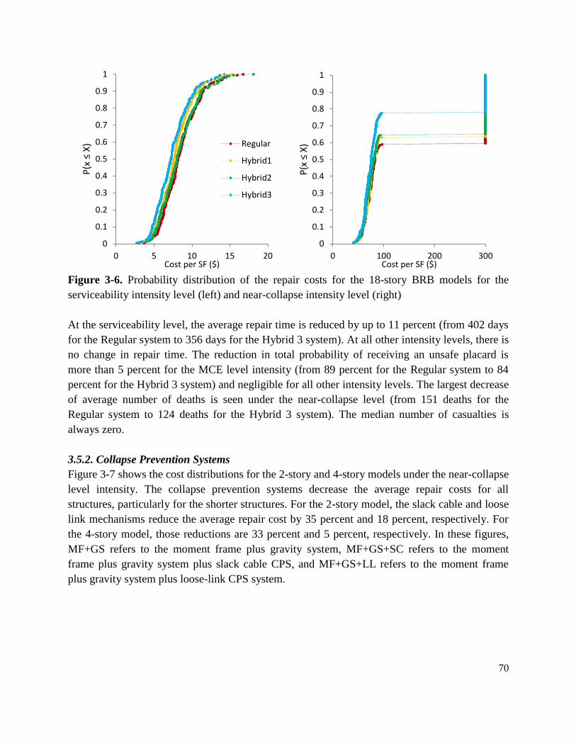
70



At the serviceability level, the average repair time is reduced by up to 11 percent (from 402 days

for the Regular system to 356 days for the Hybrid 3 system). At all other intensity levels, there is

no change in repair time. The reduction in total probability of receiving an unsafe placard is

more than 5 percent for the MCE level intensity (from 89 percent for the Regular system to 84

percent for the Hybrid 3 system) and negligible for all other intensity levels. The largest decrease

of average number of deaths is seen under the near-collapse level (from 151 deaths for the

Regular system to 124 deaths for the Hybrid 3 system). The median number of casualties is

always zero.

3.5.2. Collapse Prevention Systems

Figure 3-7 shows the cost distributions for the 2-story and 4-story models under the near-collapse

level intensity. The collapse prevention systems decrease the average repair costs for all

structures, particularly for the shorter structures. For the 2-story model, the slack cable and loose

link mechanisms reduce the average repair cost by 35 percent and 18 percent, respectively. For

the 4-story model, those reductions are 33 percent and 5 percent, respectively. In these figures,

MF+GS refers to the moment frame plus gravity system, MF+GS+SC refers to the moment

frame plus gravity system plus slack cable CPS, and MF+GS+LL refers to the moment frame

plus gravity system plus loose-link CPS system.

0

0.1

0.2

0.3

0.4

0.5

0.6

0.7

0.8

0.9

1

0 5 10 15 20

P(x

≤ X

)

Cost per SF ($)

Regular

Hybrid1

Hybrid2

Hybrid3

0

0.1

0.2

0.3

0.4

0.5

0.6

0.7

0.8

0.9

1

0 100 200 300

P(x

≤ X

)

Cost per SF ($)

71

Figure 3-7. Probability distribution of the CPS repair costs for the near-collapse level intensity

for the 2-story models (left) and 4-story models (right)

For all the models, the collapse prevention systems have negligible effect on the average repair

time and total probability of receiving an unsafe placard. However, the average number of

casualties is significantly decreased in many cases. The reduction from the slack cable

mechanism is more than 32 percent for the 2-story model and nearly 15 percent for the 4-story

model, and the reduction from the loose link mechanism is nearly 15 percent for the 2-story

model and nearly 7 percent for the 4-story model. The median number of casualties is zero for all

the models.

3.5.3. Special Moment Frames Modeled With and Without Gravity Systems

Like for the BRB systems, the results are presented in the order of the number of total stories,

starting with the two story systems, and the cost distributions are plotted for the intensity with

the least improvement between systems and for the intensity with the most improvement

between systems. Figure 3-8 shows example cost distributions for the 2-story models at the

serviceability level and the MCE levels. For this model, the largest improvement in average cost

can be seen at the higher intensity levels. The average cost was decreased by more than 12

percent under the DBE level, by 21 percent under the MCE level, and by nearly 18 percent under

the near-collapse level intensity. Under the serviceability levels, the average cost actually

increased up to 10 percent when the partially restrained connections are modeled. This is due to

the sensitivity of the nonstructural components to small changes in acceleration values. The

accelerations experienced by the models with the gravity system at certain stories were

occasionally higher than the models with no gravity system resistance. While these changes in

acceleration were not excessive, they are reflected in the nonstructural costs during the

realizations with higher total costs. Since the nonstructural components have a strong influence

0

0.1

0.2

0.3

0.4

0.5

0.6

0.7

0.8

0.9

1

0 100 200 300

P(x

≤ X

)

Cost per SF ($)

MF+GS

MF+GS+SC

MF+GS+LL

0

0.1

0.2

0.3

0.4

0.5

0.6

0.7

0.8

0.9

1

0 100 200 300

P(x

≤ X

)

Cost per SF ($)

MF+GS

MF+GS+SC

MF+GS+LL

72

in the consequences at the serviceability levels, this phenomenon is more prevalent at the lower

intensities. The results between the two levels of gravity connection strengths are similar, and the

higher strength does not necessarily cause a larger decrease in consequences.

Figure 3-8. Probability distribution of the repair costs for the 2-story SMRF models for the

serviceability intensity level (left) and MCE intensity level (right)

The repair time is decreased by more than 6 percent under the DBE level (from 355 days for the

0GS system to 345 days for the 35GS); the change is negligible for all other intensities. The

probability of receiving an unsafe placard is decreased by 8 percent under the DBE level (from

98 percent for the 0GS system to 90 percent for the 50GS); the change is negligible for all other

intensities. For all models, the average number of casualties is negligible. The median number of

collapses is zero, except under the near-collapse level intensity. In this case, the median number

of casualties is always around 1.0.

Figure 3-9 shows example cost distributions for the 4-story models at the serviceability level and

the near-collapse levels. Like the 2-story model, the largest improvement can be seen at the

higher intensity levels. The average cost was decreased by 17 percent under the DBE level, by 29

percent under the MCE level, and by nearly 32 percent under the near-collapse level intensity.

Under the serviceability levels, the average cost actually increased up to 7 percent when the

partially restrained connections are modeled. The results between the two levels of gravity

connection strengths are similar, but the higher strength does cause a larger decrease in cost for

this structure.

0

0.1

0.2

0.3

0.4

0.5

0.6

0.7

0.8

0.9

1

0 20 40 60

P(x

≤ X

)

Cost per SF ($)

0GS

35GS

50GS

0

0.1

0.2

0.3

0.4

0.5

0.6

0.7

0.8

0.9

1

0 100 200 300

P(x

≤ X

)

Cost per SF ($)

0GS

35GS

50GS

73



The changes in repair time and probability of receiving an unsafe placard for the 4-story model

are negligible. The average number of casualties is reduced under the larger intensities. This

reduction is up to 11 percent under the MCE and up to 23 percent under the near-collapse level

intensity (from 33 deaths for the 0GS system to 26 deaths for the 50GS). The median number of

collapses is always zero.

Figure 3-10 shows example cost distributions for the 8-story models at the serviceability level

and the near-collapse levels. Like the previous models, the largest improvement can be seen at

the higher intensity levels, but the average costs decrease at all intensity levels. The average cost

was decreased by more than 3 percent under the serviceability level, by 10 percent under the

DBE level, by nearly 10 percent under the MCE level, and by nearly 11 percent under the near-

collapse level intensity. These reductions at the higher intensities are less than those for the

shorter structures. The changes in repair time, probability of receiving an unsafe placard, and

number of casualties for the 8-story mode are negligible. The median number of collapses is

zero, except under the DBE level intensity. In this case, the median number of casualties is 7

deaths.

0

0.1

0.2

0.3

0.4

0.5

0.6

0.7

0.8

0.9

1

0 10 20 30 40

P(x

≤ X

)

Cost per SF ($)

0GS

35GS

50GS

0

0.1

0.2

0.3

0.4

0.5

0.6

0.7

0.8

0.9

1

0 100 200 300

P(x

≤ X

)

Cost per SF ($)

0GS

35GS

50GS

74



3.6. Summary and Conclusions

This research provides comparative analyses of new and traditional seismic resisting systems and

modeling methodologies, shows the results of those analyses in terms of consequence, and gives

numerous examples of the P-58 methodology. The results presented show how changes to the

design or modeling of a system can have substantial influence in the behavior at multiple

intensity levels. The results are presented in terms of repair costs, repair times, number of

casualties, and probability of receiving an unsafe placard, which are more meaningful to owners

and other decision makers. The innovative systems discussed here can provide significant benefit

to the lateral resistance of a structure when analyzed using the principles of Performance Based

Earthquake Engineering.

The first innovative system, the Hybrid BRBs, use a multi core system with steels of different

strengths. These various strengths are used to control the sequence of yielding, and with a

minimum change to the design of BRBs, the behavior can be significantly modified. When

compared to traditional BRB systems, the repair costs are reduced by up to 12 percent at lower

intensity levels for short structures and up to 26 percent at higher intensities for the taller

structures. Additionally, the repair time at the serviceability level is always reduced by more than

10 percent. In general, there was negligible change in the probability of receiving an unsafe

placards and the number of casualties. The more hybridity in the BRB, the more the

consequences are reduced. This trend was similar to those found in the P-695 analyses (Atlayan

and Charney 2013), where the Hybrid 3 system always had the smallest probability of collapse

and residual drifts. While residual drifts were not included in the P-58 analyses (again, to prevent

the loss of “true data”), one of the major benefits found in the P-695 analyses of the Hybrid

0

0.1

0.2

0.3

0.4

0.5

0.6

0.7

0.8

0.9

1

0 10 20 30

P(x

≤ X

)

Cost per SF ($)

0GS

35GS

50GS

0

0.1

0.2

0.3

0.4

0.5

0.6

0.7

0.8

0.9

1

0 100 200 300

P(x

≤ X

)

Cost per SF ($)

0GS

35GS

50GS

75

BRBs was the reduction in residual drifts. If these were included in the P-58 analyses, the

consequences would likely be reduced even more with the hybrid systems.

The Collapse Prevention System is designed specifically for life safety in locations where that is

the only crucial intensity level, like the Central and Eastern United States. In the CEUS, large

rare ground motions must be designed for, but more frequently occurring ground motions are

negligibly small. The collapse prevention mechanisms are added to the gravity system and

remain inactive until the structure reaches a specified level of drift. At the near-collapse level,

the average repair costs are always decreased by 5 to 36 percent when the collapse prevention

mechanism is added. This reduction was greater for buildings with fewer stories and was greater

for the slack cable device than the loose link device. For the 2-story model, the average number

of casualties was significantly decreased (nearly 33 percent) by the slack cable mechanism. In

general, there was negligible change in the repair time and the probability of receiving an unsafe

placard. If a detailed cost analysis is done on the systems, it is likely that the Collapse Prevention

Systems will have a lower initial cost than the comparable seismic resisting system, due to the

lack of seismic detailing. Collapse Prevention systems that use non-ductile moment frames do

not have demand-critical field welding, and they have fewer and less difficult special inspections

when compared to welded ductile moment frames. With this in mind, the reduction in repair cost

would likely be even more significant than shown in this work.

Including the lateral resistance from the gravity systems is a modeling assumption, instead of an

innovative system like the previous two systems. By modeling this lateral resistance, the average

costs can be reduced significantly (up to 32 percent), particularly at higher intensity levels. For

the 4-story model, the number of casualties was noticeably reduced at higher intensities;

otherwise, all other consequences had negligible change. It should be noted that these

consequence reductions may be unconservative, due to the simplistic nature of the modeling of

the partially restrained connections.

3.7. Recommendations and Future Work

The Hybrid Buckling Restrained Braces could be used where traditional Buckling Restrained

Braces are acceptable. With a minimal change to the design of the BRB, the Hybrid BRBs can

significantly reduce the consequences, particularly the repair costs, under multiple intensities.

The collapse prevention systems, on the other hand, should be used in locations where the

seismicity is controlled only by large, rare events. These systems provide a mechanism that only

activates under large drifts to reduce the number of collapse and the consequences at these high

intensities. The lateral strength and resistance of the gravity system could be included if the

engineers wants a more accurate estimation of consequences from the mathematical model.

76

Additional analyses should be run with new structural configurations to determine how the

trends expand to a wide variety of uses. The P-58 analyses for the Hybrid BRBs should be run

with the residual drift inputs to determine the additional decrease in consequences, and the P-58

analyses of the Collapse Prevention Systems should be run with a more accurate cost estimate to

determine the additional decrease in consequences. Additionally work should be done to improve

the modeling of the gravity system connections. Simplistic models and limited test data result in

a modeling methodology that may not be sufficient to capture the true behavior of the gravity

connections.

While the PACT program includes a wide variety of fragilities, there are still numerous

components in a typical building that do not have fragilities developed. For a more accurate

estimation of consequences, these fragilities would need to be developed. Additionally, the cost

estimates in PACT are based on 2011 estimates. These will need to be updated on a regular

basis, or the P-58 procedure could become obsolete in a few years. These systems could also be

analyzed for a specific location using a time-based assessment to see location specific benefits.

77

Chapter 4: “Response-History Analysis for the Design of New Buildings: A

Study of Assumptions”

Jordan A. Jarrett, Reid B. Zimmerman, Finley A. Charney, Afshar Jalalian

[To Be Submitted to Earthquake Spectra]

Abstract

Numerous assumptions are made when developing methodologies for nonlinear response history

analyses. The accuracy of several assumptions is investigated using proposed changes to Chapter

16 of ASCE 7. The major findings of this work include: (1) Modeling the gravity system’s lateral

influence can have significant effect on the system behavior but is unnecessary unless a more

accurate representation of the behavior is needed. (2) Exclusion of a residual drift check is

acceptable when concerned with collapse prevention. (3) Spectrally matched ground motions

should cautiously be used for near-field structures. (4) The effects of nonlinear accidental torsion

can be influential, but there are insufficient studies to warrant modification of existing code

language at this time. (5) Even if a structure is designed per ASCE 7, it may not have the

assumed probability of collapse under the maximum considered earthquake when analyzed using

FEMA P-695.

4.1. Introduction

4.1.1. Summary of Proposed ASCE 7 Chapter 16 Provisions

The Building Seismic Safety Council Response History Analysis Issue Team has proposed

changes for the next update of Chapter 16 for ASCE 7-16, which encompasses nonlinear

response history analysis of building structures (Haselton et al. 2013). More than a minor update

from ASCE 7-10, the proposed Chapter 16 for ASCE 7-16, hereinafter referred to simply as

Chapter 16, makes significant changes to and replaces large portions of the existing provisions,

which were identified as outdated and in some cases unclear. An introduction to these changes

will be discussed here, but a more complete description of the development and application of

the ASCE 7 Chapter 16 provisions can be found elsewhere (Haselton et al. 2013, Zimmerman et

al. 2013).

The seismic hazard for Chapter 16 is set at the risk targeted maximum considered earthquake

(MCER) level, instead of the design basis earthquake. Additionally, two methods are proposed

for the MCER design spectrum. The first is the traditional code-based spectrum developed for

MCER with or without site-specific procedures, as described in Chapter 21 of ASCE 7-10 (ASCE

78

2010). The second proposed method requires the development of two or more conditional spectra

(Haselton et al. 2013).

A suite of eleven record sets for the traditional code-based spectrum, or one suite of eleven

record sets for each conditional spectra, is defined as the minimum number of records. This new

requirement replaces the old provisions of using a suite of three or more record sets. The chosen

record sets should be consistent with the tectonic setting, magnitude and distance controlling the

seismic hazard at the site and should have a spectrum that closely follows the target spectral

shape. Simulated ground motions are considered acceptable, especially to fill any gaps where

recorded motions are scarce. Chapter 16 additionally requires that ground motions used for near-

fault sites include rupture directionality, velocity pulses, and fling step. Spectral matching is also

permitted; however, the scaling requirements are different than those of amplitude-scaled and

simulated ground motions.

Scaling of ground motions has been changed, motivated by the switch from a geometric mean to

a maximum direction target spectrum. Instead of combining the two ground motion components

using the square-root-of-the-sum-of-the-squares (SRSS) method, a maximum direction spectrum

for each motion must be constructed, either by using the period-dependent scale factors, such as

those listed in Table C21.2-1 of the 2009 NEHRP Recommended Seismic Provisions (FEMA

2009c), or by direct computation through rotation of the motion over all angles. The average

over the suite of these maximum direction spectra must fit the target spectrum on average and

cannot fall below 0.9 times the ordinate of the target spectrum within the period range of interest.

If spectrally matched ground motions are used, the average of all the individual components

must not fall below the target spectrum within the period range of interest. Due to the scaling of

individual components rather than maximum direction spectra, this requirement adds an implicit

penalty to spectral matching in these procedures. For near-fault sites, the as-recorded fault

normal and fault parallel ground motion components must be applied in the fault normal and

fault parallel directions at the site considering the controlling fault orientation. For non–near-

fault sites, the ground motions are applied in arbitrary orientations.

Modeling requirements remain general, similar to previous provisions, with a few additions and

modifications. These modifications include the designation of force and deformation controlled

elements, a cap on inherent viscous damping, clearer provisions on soil-structure interaction, the

required use of expected strengths, and removal of multiple gravity load conditions. Chapter 16

also gives the analyst the choice of directly modeling the stiffness and strength of the gravity

system and does not require consideration of accidental torsion in the nonlinear analyses. Three-

dimensional models are required, and thus, two-dimensional mathematical models will no longer

be allowed.

79

The acceptance criteria, on the other hand, have been significantly modified. Chapter 16 still

references testing and relies on other standards for specific values of acceptance criteria (PEER

2010, ASCE 2006), but provides a framework over which the available information can be

translated into ASCE 7 checks. It does this by separating acceptance criteria into global and local

designations, with the former including provisions for drift and the case of unacceptable response

and the latter encompassing force- and deformation-controlled elements. Drift limits are taken

from ASCE 7 Chapter 12 and modified for nonlinear response history analysis results at MCER

level ground motions. An unacceptable response is defined as any ground motion that causes

dynamic instability, non-convergence, exceedance of the valid range of modeling for

deformation controlled actions, or exceedance of capacity in critical force controlled actions. The

provisions require that for Risk Category I and II structures, analyzed without spectral matched

ground motions, no more than one in eleven motions can cause an unacceptable response. For

Risk Category III and IV structures, no unacceptable responses are allowed. Deformation-

controlled actions must additionally not exceed a given proportion of the point at which vertical

load-carrying capacity is lost, while amplified force-controlled action demands may not exceed

the corresponding strength capacity. The proportion for deformation-controlled and amplification

for force-controlled actions depend on the severity of the failure with critical elements being

those where failure should lead to local or global collapse. Examples of force- and deformation-

controlled actions include axial force in columns and plastic rotation of beam-column

connections, respectively.

The Chapter 16 methodology is assumed to implicitly satisfy a 10 percent probability of collapse

under the MCER level ground motion for Risk Category I and II, as described in Table C.1.3.1b

in ASCE 7-10 (ASCE 2010). This level of probability was originally recommended in the FEMA

P-695 methodology (FEMA 2009a) and then later adopted for ASCE 7. For a Risk Category III

structure, this probability is reduced to 6 percent, and for a Risk Category IV structure, it is

reduced further to 3 percent.

4.1.2. Description of Assumptions Investigated

The proposed Chapter 16 provides a more comprehensive methodology for nonlinear response

history analysis and related acceptance criteria of structures compared to the existing provisions

(ASCE 2010). During its development, however, numerous assumptions have been made that

require further investigation. This work highlights several aspects of the proposed update,

including: (1) the influence of the inclusion of the lateral strength and stiffness of the gravity

system, (2) the practicality of a residual drift check, (3) the applicability of spectrally matched

ground motions, (4) the necessity of a nonlinear accidental torsion check, and (5) the accuracy of

the assumed implicit satisfaction of a specified percent probability of collapse under the MCER

level ground motion. It is important to note that the conclusions made in this research could be

80

applicable to any methodology that uses nonlinear response history analysis, even though the

basis is the proposed Chapter 16.

The first provision investigated is the effect that the stiffness and strength of the gravity framing

system can have on satisfaction of the Chapter 16 provisions. Gravity systems are rarely included

in analytical models for response history analysis, other than to capture P-Delta effects or

identified interactions where gravity systems are thought to affect the demands on the lateral

system. It is typically believed to provide conservative results when the gravity systems are

omitted. In reality, this inclusion could provide more accurate results, since historical evidence

has shown that the gravity system can provide significant resistance during earthquakes. For

example, during the 1994 Northridge earthquake, many special moment frame connections

developed brittle failures; however, these buildings did not collapse, in part because the gravity

system provided additional seismic resistance (Lui and Astaneh-Asl 2000, Green et al. 2004).

Including all the aspects of lateral strength and stiffness of the gravity system would provide a

more realistic model and response. However, there is little agreement within differing provisions

on how to handle the modeling of the gravity system. The FEMA P-58 methodology states that

all elements that provide lateral resistance should be included, but it does not give a definite

recommendation of the inclusion of the gravity system (FEMA 2012). The Tall Building

Initiative recommends the inclusion of the gravity system resistance (PEER 2010), while the

gravity system is never modeled when using the traditional P-695 methodology (FEMA 2009a).

However, in the Appendix F methodology of FEMA P-695, which is discussed in more detail

later, the modeling of the gravity system is recommended. Chapter 16 does not require explicit

modeling of the gravity system unless it significantly affects the seismic response under the

MCER ground motions; however, the influence of the gravity system resistance is likely not

known unless it is modeled. Due to this concern, the effects of this provision are investigated in

this study.

In some performance-based design guidelines such as the Tall Building Initiative (PEER 2010)

and the FEMA P-58 methodology (FEMA 2012), calculation of residual drifts is required. For

the Tall Building Initiative, the mean residual drift ratio from a suite of ground motion records

may not exceed 1 percent. Residual drifts are a key factor in procedures used to determine the

post-earthquake capacity of a structure (Bazzurro et al. 2004), and high residual drifts often mean

that it is more economically feasible to demolish the damaged structure than to repair it

(McCormick et al. 2008, Ruiz-Garcia and Miranda 2010). However, studies have also shown that

the magnitude of residual drifts rarely relates to collapse under typical aftershock events (Lee

and Foutch 2004). Since Chapter 16 is mostly concerned with collapse prevention, it does not

require a check on residual drifts. This study will determine if residual drift can be linked in any

way to collapse, which would warrant the inclusion of a residual drift check.

81

The third assumption investigated is the acceptability of using tight spectral matching to modify

ground motions, which is an option in the updated Chapter 16. In this paper, tight spectral

matching is defined as frequency-modification of recorded ground motion acceleration time

histories such that the resulting response spectrum fits a pre-determined target spectrum with

little deviation over a selected period range. Tight spectral matching is the most common form of

a broader class of spectral matching techniques and is often employed by practicing geotechnical

engineers when providing ground motion time histories for the design of buildings. The

appropriateness of tight spectral matching is heavily debated in the literature with well-founded

arguments in support of and against using matched ground motions (NIST 2011, Hancock et al.

2008, Bazzuro and Luco 2006). Since this debate is extensive in the literature, it is not the intent

of the authors to provide a final conclusion on this matter but rather to explore how tight spectral

matching specifically affects the results of the updated Chapter 16 through several case studies.

If spectrally matched ground motions generated by the Chapter 16 provisions produce

comparable results to those of amplitude scaled motions, then it is likely that they are suitable if

the design engineer choses to use them.

The effect of accidental torsion is investigated to determine the necessity for such a check within

nonlinear response history analyses. Accidental torsion is typically ignored in performance-based

earthquake engineering provisions, including the P-695 procedure (FEMA 2009a), the P-58

procedure (FEMA 2012) and the Tall Building Initiative (PEER 2010). However, this accidental

torsion has been shown to have a significant effect on the inelastic behavior of structures

(Mansuri 2009), which could warrant a check for accidental torsion within a nonlinear response

history procedure. One method to assess accidental torsion is to extend linear procedures such as

those that exist in ASCE 7 Chapter 12 (ASCE 2010) and ASCE 41 (ASCE 2006), where the

center of mass is shifted 5 percent of the diaphragm dimension in each direction independently,

to nonlinear procedures. Studies have shown that the uncertainty in the center of mass is

typically the largest influence to accidental torsion (De la Llera and Chopra 1995), which is

likely why the 5 percent offset procedure is typically used. The practical concern for response

history analysis is that the shifts in mass quadruples the number of analyses performed, since the

structure must be analyzed with the four shifted center of mass locations. The research presented

herein will investigate whether accidental torsion should be included in the nonlinear analysis.

The final assumption investigated is the implicit satisfaction of the specified probability of

collapse when subjected to MCER motions. As discussed previously, the value of this maximum

probability of collapse is dependent on the risk category of the structure, and structures with

different risk categories are investigated in this work. Chapter 16 does not directly determine the

probability of collapse but assumes that this limit will be satisfied if all other criteria are

satisfied. The FEMA P-695 methodology, on the other hand, explicitly addresses the probability

of collapse. This methodology is further discussed in the next section, but performing both

82

methodologies on the same structure will help investigate the accuracy of this implicit

assumption of Chapter 16.

4.1.3. Summary of P-695 Methodologies

FEMA P-695 provides a methodology for determining probabilities of collapse of structures, as

well as their seismic performance factors (R, Cd, Ω0) used in design (FEMA 2009a). For this

research, the application of this methodology will focus on the determination of the probability

of collapse. There are two variations of the methodology, referred to herein as the Standard

Methodology (which is typically performed on a set of archetypes) and the Appendix F

Methodology (which is used for the evaluation of an individual structure).

The first step in either of the variations of the P-695 methodology is to determine a seismic

design category. The P-695 process has included four “location neutral” spectra that can be used

to design and analyze a structure. Once designed, a structure must be modeled, and in order to

accurately determine the collapse parameters, a detailed nonlinear model of the structure needs to

be constructed. To simulate collapse, the model should capture all significant nonlinear effects

and must include strength and stiffness degradations under large deformations. Non-simulated

collapses can be indirectly evaluated using alternative intensity level checks. A nonlinear static

pushover analysis is performed, and then nonlinear dynamic analyses are performed using one of

two scaled suites of record sets: 22 pairs of far-field ground motions or 28 pairs of near-field

motions. If the structure is within 10 kilometers of an active fault, the near-field suite should be

used; otherwise, the far-field suite is selected.

For the standard methodology, incremental dynamic analysis (IDA) is then performed by scaling

each ground motion until the structure reaches a collapse point. This analysis is used to find the

median collapse capacity, CT, which is defined as the spectral intensity at which half of the

ground motions have caused the structure to collapse or exceed the non-simulated collapse

criteria. The collapse margin ratio (CMR) is calculated as the median collapse spectral

acceleration, CT, divided by the spectral acceleration at the maximum considered earthquake,

SMT. Once the CMR has been calculated, it can be converted to the adjusted collapse margin ratio

(ACMR), which is equal to the CMR multiplied by the spectral shape factor, SSF, which is

tabulated in the methodology. The ACMR will be used along with the total dispersion, , to

determine the probability of collapse of a structure, Pc, which can be calculated as shown in

Equation 4-1. The probability of collapse is not a required calculation in the P-695 methodology,

but it can provide insight into the behavior of the structure.

∫

√

[

(

)

]

(4-1)

83

For Appendix F of P-695, incremental dynamic analysis is not used. Instead, one scale factor is

used for analysis that represents an acceptable collapse factor given a chosen maximum

probability of collapse. The normalized ground motions will all be scaled by this singular scale

factor, which is given in the methodology. Because Appendix F does not use IDA, an exact

probability of collapse cannot be calculated. However, the results will show if the probability of

collapse is above or below that limiting value.

4.2. Model Descriptions and Assumptions

4.2.1. Two-dimensional Structure Modeled with OpenSEES

The first two systems used in this study are the 2-story and 8-story steel Special Moment

Resisting Frames (SMRF) from the examples in ATC 76 (NIST 2010a), referred to hereafter as

the MF2 and MF8 Models, respectively. These frames are modeled as two-dimensional (2D)

structures in OpenSEES (McKenna 2011). In order to satisfy the modeling requirements of

Chapter 16, all nonlinear behavior of the structural system is included. The locations of nonlinear

components of the special moment resisting frames include reduced beam sections, panel zones,

column bases, and columns at moment resisting joints.

The hysteretic behavior of the reduced beam sections (RBS) is modeled using a plastic hinge and

the Modified Ibarra Krawinkler deterioration model (Lignos and Krawinkler 2010) in OpenSEES

(the Bilin material). The model used to predict the hysteretic behavior of panel zones is the

Krawinkler model (Charney and Marshall 2006). For the columns of the moment frame, a

phenomenological model that includes hinges at the bases and story joints is used to predict

deterioration. The hysteretic behavior of the columns is also modeled using the Modified Ibarra

Krawinkler deterioration model in OpenSEES. This model has the ability to account for

deterioration but not to account for P-M interaction. To include the P-M interaction, the columns

are given a reduced bending strength based on the column axial load and the P-M interaction

curve, per the guidelines in ATC 76 (NIST 2010a).

Both the MF2 and MF8 structures are modeled with and without the gravity system’s lateral

strength and stiffness. When the gravity system is included, the gravity columns are modeled

using fiber sections to check for any nonlinearity. In order to capture the full nonlinear behavior

of the gravity system, partially restrained (PR) connections are also modeled, assuming the

strength of the partially restrained connection, QCE, is lower than the plastic capacity of the beam

it is connecting. For this work, it is assumed that the strength of the partially restrained

connections is 50 percent of the strength of the beam. While this percentage may be high when

compared to true behavior, this value was taken to see the potential influence that a significant

increase in lateral strength could have on the structural behavior. Because modeling of these PR

connections can often be a complex endeavor (Rassati et al. 2004), a simple model given by

84

ASCE 41 (ASCE 2006) is used to represent the moment rotation relationship of these

connections. This model depends on the type of connection, and the “top and bottom clip angle

connection” is chosen. It is assumed that the connection angles fail due to flexure.

Since both the MF2 and MF8 Models are represented in 2D, floor constraints connect the frames

acting in the same direction. P-Delta effects for models without the gravity system are modeled

with a leaning column; for models that include the gravity system, P-Delta effects are satisfied

by the explicit inclusion of the gravity columns.

4.2.2. Three-dimensional Structure Modeled with Perform-3D

The three-dimensional model used in this paper, referred to hereafter as the 3D Model, is

described completely elsewhere and is representative of an actual Risk Category III commercial

building (Zimmerman et al. 2013). Its lateral force-resisting system consists of two lines of steel

special moment-resisting frame (SMRF) in the longitudinal direction and four lines of buckling-

restrained brace frame (BRBF) in the transverse direction over five stories. The lowest story

relies on reinforced concrete walls around the building perimeter. Each floor has a rigid

diaphragm constraint applied, except the first floor where the diaphragm flexibility is explicitly

modeled. The SMRF and BRBF directions align with the fault normal and fault parallel

components of ground motion, respectively. A leaning column is provided to capture the P-Delta

effects arising from vertical loads acting on the excluded gravity system. Foundation flexibility

and consideration of soil-structure interaction effects were not explicitly considered.

Extensive nonlinear modeling is employed in Perform 3D (CSI 2011), including localized axial-

moment-moment (PMM) interacting hinges for SMRF and BRBF columns, moment-rotation

hinges for SMRF beam-column connections and BRBF beams outside of gusset plates, buckling-

restrained brace (BRB) elements and inelastic shear stress-shear strain material models for concrete

walls. Values for plastic displacements at which vertical load-carrying capacity is lost for use in

Chapter 16 deformation acceptance criteria checks are taken from ASCE 41 (ASCE 2006), testing

(SSDA 2001), and a study conducted by Rutherford + Chekene (R+C 2011). The plan view of the

Perform 3D model of the structure is found in Figure 4-1.

85

Figure 4-1. Schematic of the lateral force-resisting system of the 3D Model

4.3. Ground Motion Selection and Scaling

4.3.1. Design Spectra for 2D Models

The code spectrum used for the design and analysis of the special moment resisting frames is the

FEMA P-695 Dmax spectrum, which is defined in the methodology and is based on the ASCE 7-

05 design spectra (ASCE 2005). Since the MF2 and MF8 Models are analyzed in 2D, only

individual ground motion components are used, and the scaling procedures are similar to those

laid out for spectrally matched ground motions. Each individual component is scaled such that

the average never falls below the design spectrum. The same ground motions are used as seeds

for the creation of a suite of tight spectrally matched ground motions, which are created with the

program RSPMatch (Al Atik and Abrahamson 2010). As an example of the scaling procedure,

Figure 4-2 shows the response spectra of those components after amplitude scaling (SCAL) and

after spectrum matching (MTCH) for the MF2 Models. For the MF8 Model, the same spectrum

is used, but the period range considered is changed to 0.46 seconds through 4.6 seconds.

Figure 4-2. The response spectra of the amplitude scaled ground motions components (left) and

the spectrum matched components (right) versus the target spectrum for the MF2 Model

0

0.5

1

1.5

2

2.5

3

0 0.5 1 1.5 2 2.5 3 3.5 4

Sp

ectr

al a

ccel

erat

ion

[g]

Period [s]

Single component spectra

Target spectrum

Average

Period range considered

0

0.5

1

1.5

2

2.5

3

0 0.5 1 1.5 2 2.5 3 3.5 4

Sp

ectr

al a

ccel

erat

ion

[g]

Period [s]


Target spectrum

Average


B

RB

F

B

RB

F

B

RB

F

SMRF

SMRF B

RB

F

86

4.3.2. Design Spectra for 3D Model

A site-specific MCER target spectrum was developed for the near-fault site of the 3D Model in

Berkeley, California. Due to the proximity to the Hayward Fault, the target response spectrum is

deterministically capped by the 80 percent lower limit of ASCE 7 Section 21.3 (ASCE 2010).

Figure 4-3 presents the maximum direction spectra for the scaled suite (SCAL) and the single

component spectra for the spectrally matched suite (MTCH).

Figure 4-3. Maximum direction spectra versus the target spectrum for SCAL suite (left) and the

component spectra versus the target spectrum for the MTCH suites (right) of the 3D Model

In addition to the code-based target spectrum, two scenario or conditional spectra were

developed for the 3D Model. To capture the predominant periods of response and satisfy the

Chapter 16 requirements, two conditional spectra were chosen, one conditioned at a period of 0.5

seconds and the other at 2.0 seconds. These spectra are developed such that the envelope of the

scenario spectra is more than 75 percent of the site-specific MCER spectrum within the period

range of interest. Two suites of eleven motions, one for each spectrum, were then selected and

scaled. In accordance with Chapter 16, results from both suites must satisfy all requirements for

the structure to be deemed acceptable under the provisions. This is in contrast to using the

amplitude scaled or spectrum matched suites, where only one suite of ground motions needs to

provide acceptable results. Figure 4-4 presents the maximum direction spectra for the conditional

spectra at 0.5 seconds (05CS) and for the conditional spectra at 2.0 seconds (20CS). A more

detailed description of spectrum and ground motion development can be found elsewhere

(Zimmerman et al. 2013).

0

0.5

1

1.5

2

2.5

3

0 0.5 1 1.5 2 2.5 3 3.5 4

Sp

ectr

al a

ccel

erat

ion

[g]

Period [s]

Maximum direction spectra

Target spectrum

Average


0

0.5

1

1.5

2

2.5

3

0 0.5 1 1.5 2 2.5 3 3.5 4

Sp

ectr

al a

ccel

erat

ion

[g]

Period [s]


Target spectrum

Average


87

Figure 4-4. Maximum direction spectra for the 05CS (left) and 20CS (right) suites versus the

target spectrum of 3D Model

4.4. Gravity System Modeling Study Results

To investigate the influence of the lateral resistance of the gravity system, both moment frame

systems (MF2 and MF8 Models) are modeled with and without this influence. Since the 3D

Model has excluded the gravity system, that structure is not addressed in this section. This

section provides a discussion on the effects of modeling the gravity system as well as an overall

example application of the proposed Chapter 16 methodology. The story drift ratios are

presented to investigate the influence of including the lateral strength and stiffness of the gravity

system. Using the drift limits in ASCE 7 Chapter 12 (ASCE 2010) and assuming Risk Category

II, the allowable story drift ratios for moment frames are 2 percent of the story height. Chapter

16 drift acceptance criteria states that the suite mean story drift ratio should not exceed 2.0 times

the drift ratio limits from Chapter 12, which for these moment frames equals 4 percent.

As mentioned previously, the 2D structures are modeled with and without the lateral resistance

of the gravity system. Chapter 16 allows the user to determine whether or not to consider the

gravity system influence. Figure 4-5 shows the mean drift ratios for the four analyses run on the

2D Models: with or without gravity system and under the SCAL or MTCH suites. Each line on

the graph represents the suite mean drift ratio (the average of the maximum drift ratio over all

eleven ground motions in each suite).

For the MF2 Model, it is important to note that one instability occurs under the SCAL suite when

the strength and stiffness of the gravity system was excluded, which results in a change in the

acceptance criteria per the proposed Chapter 16. In this case, the larger of 1.2 times the median

of the eleven motions or the mean of the remaining ten motions is compared against the limit.

For the MF2 Model under the SCAL suite, 1.2 times the median produces the largest drift ratios,

which are 0.042 and 0.038 for the first and second stories, respectively. This first floor drift ratio

0

0.5

1

1.5

2

2.5

3

0 0.5 1 1.5 2 2.5 3 3.5 4

Sp

ectr

al a

ccel

erat

ion

[g]

Period [s]


Target spectrum

Average


0

0.5

1

1.5

2

2.5

3

0 0.5 1 1.5 2 2.5 3 3.5 4

Sp

ectr

al a

ccel

erat

ion

[g]

Period [s]


Target spectrum

Average


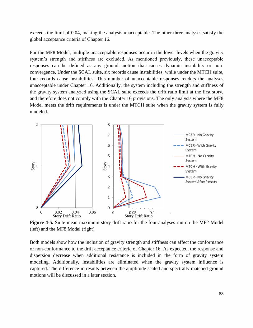
88

exceeds the limit of 0.04, making the analysis unacceptable. The other three analyses satisfy the

global acceptance criteria of Chapter 16.

For the MF8 Model, multiple unacceptable responses occur in the lower levels when the gravity

system’s strength and stiffness are excluded. As mentioned previously, these unacceptable

responses can be defined as any ground motion that causes dynamic instability or non-

convergence. Under the SCAL suite, six records cause instabilities, while under the MTCH suite,

four records cause instabilities. This number of unacceptable responses renders the analyses

unacceptable under Chapter 16. Additionally, the system including the strength and stiffness of

the gravity system analyzed using the SCAL suite exceeds the drift ratio limit at the first story,

and therefore does not comply with the Chapter 16 provisions. The only analysis where the MF8

Model meets the drift requirements is under the MTCH suite when the gravity system is fully

modeled.

Figure 4-5. Suite mean maximum story drift ratio for the four analyses run on the MF2 Model

(left) and the MF8 Model (right)

Both models show how the inclusion of gravity strength and stiffness can affect the conformance

or non-conformance to the drift acceptance criteria of Chapter 16. As expected, the response and

dispersion decrease when additional resistance is included in the form of gravity system

modeling. Additionally, instabilities are eliminated when the gravity system influence is

captured. The difference in results between the amplitude scaled and spectrally matched ground

motions will be discussed in a later section.

0

1

2

0 0.02 0.04 0.06

Sto

ry

Story Drift Ratio

0

1

2

3

4

5

6

7

8

0 0.05 0.1

Sto

ry

Story Drift Ratio

89

4.5. Residual Drift Study Results

Chapter 16 remains does not require a check on residual drifts, and the following studies intend

to analyze this parameter for structures that otherwise satisfy the provisions.

4.5.1. MF2 and MF8 Models Results

Figure 4-6 shows the suite mean residual drifts for all four analyses of the MF2 and MF8

Models. The suite mean residual drift ratios follow similar trends to the suite mean drift ratios.

For the MF2 Model, the ratio between the residual drift and mean drift ratios varies from 20

percent to more than 50 percent. For the MF2 Models that satisfied the Chapter 16 criteria (all

except the system without gravity influence under the SCAL suite), the residual drift ratios

approach 1 percent, and the standard deviation can also be significant. For the MF8 Model, the

ratio between the suite mean residual drift ratios and the suite mean drift ratios varies from 5

percent to above 50 percent on the top six levels. In the bottom two levels, this ratio can exceed

90 percent, although that is a result of multiple instabilities at those levels.

Figure 4-6. Suite mean residual drifts for the analyses of MF2 Model (left) and the MF8 Model

(right)

Similar to the mean drift ratios, the mean residual drift ratios typically decrease when the gravity

system strength and stiffness are modeled. Typically, the spectrally matched ground motions

cause a significant decrease in both the residual drift ratios and the ratio between the residual and

maximum drift ratios. The one exception is the MF2 Model when the gravity system resistance is

included, when the SCAL and MTCH suites produce very similar results.

0

1

2

0 0.01 0.02 0.03

Sto

ry

Mean Residual Drift

0

1

2

3

4

5

6

7

8

0 0.05 0.1 0.15

Sto

ry

Mean Residual Drift

SCAL - No Gravity System

SCAL - With Gravity System

MTCH - No Gravity System

MTCH - With Gravity System

90

4.5.2. 3D Model Results

Suite mean story drift ratios are shown in Figure 4-7 superimposed over the drift limit from

Chapter 16. For a Risk Category III structure, the story drift ratio limit in ASCE 7 Chapter 12 is

1.5 percent. Chapter 16 thus allows a maximum drift ratio of twice that or 3 percent. Note that an

unacceptable response occurred in the 05CS suite. Although an unacceptable response is not

permitted per Chapter 16 for a Risk Category III structure, the Chapter 16 procedure for when

one does occur has been applied here in order to report the global drifts for the 05CS suite.

Therefore the 05CS suite “mean” is reported as the maximum of the mean of the remaining ten

motions or 1.2 times the median of the full suite. All other suite means are calculated as the mean

of the full suite. It is observed in Figure 4-7 that the SCAL suite mean in the SMRF direction

exceeds the limit in two stories while all other suites pass this check. The conditional spectra

suites tend to produce much smaller suite mean drifts than the SCAL and MTCH suites for both

directions. As noted in the following section entitled “Spectral Matching of Ground Motions

Study Results”, the SCAL suite tends to exceed the MTCH suite results in the SMRF direction

and vice versa in the BRBF direction.

Figure 4-7. Suite mean maximum story drift ratio for the 3D Model in the SMRF (left) and

BRBF (right) direction

The residual story drift ratios are shown in Figure 4-8. Due to the occurrence of dynamic

instability in the 05CS suite, the suite mean is shown as the mean of the remaining ten motions.

All other suite means are calculated as the mean of the full suite. The distribution of residual

story drift ratios over the height closely matches that of story drift ratios. The residual drift ratios

can get as high as 50 percent of the maximum drift ratios in some cases.

0

1

2

3

4

5

6

0 0.01 0.02 0.03 0.04

Sto

ry

SMRF Mean Story Drift Ratio

0

1

2

3

4

5

6

0 0.01 0.02 0.03 0.04

Sto

ry

BRBF Mean Story Drift Ratio

SCALMTCH05CS20CSLimit

91

In general, the magnitude of the suite mean residual story drift ratios for the 05CS and 20CS

suites are less than those of the SCAL and MTCH, consistent with the fact that magnitude of

mean story drift ratios were less for the 05CS and 20CS suites. Story drifts in the BRBF direction

also tend to be smaller in magnitude than the SMRF direction owing to the properties of each

respective system. It is of special note that even for a structure complying with Chapter 16, the

residual drift ratios can be significant as evidenced by more than 1 percent in the SMRF direction

under the SCAL suite. Although not shown, the dispersion within a suite of residual drift ratio

tends to be quite large. In many cases, the suite mean residual drift ratio is skewed due to one or

two ground motions that produce larger than average residual drifts such as the SCAL suite in

the SMRF direction of Figure 4-8.

Figure 4-8. Suite mean residual story drift ratio for the 3D Model in the SMRF (left) and BRBF

(right) direction

4.5.3. Residual Drift Incremental Dynamic Analyses

To determine the potential consequences of residual drift, incremental dynamic analyses (IDA)

are performed on selected ground motions that caused significant residual roof drift (greater than

or equal to 1 percent) but no dynamic instability. The ground motion accelerations were

increased in 10 percent increments up to 150 percent of their original scaling to determine how

close the structures are to collapse. Figure 4-9 shows the IDA residual drift results, and the initial

residual drift from each ground motion record is the x-intercept. Due to the higher initial residual

drifts, this investigation was performed on the MF2 and MF8 Models that do not include

modeling of the gravity system resistance and in the SMRF direction of the 3D Model.

Nine of the thirteen ground motions caused a collapse at or before a scale factor of 1.5; however,

the ground motion needed to be scaled by a factor of at least 1.2 percent to cause collapse.

0

1

2

3

4

5

6

0 0.005 0.01 0.015 0.02

Sto

ry

SMRF Mean Story Drift Ratio

0

1

2

3

4

5

6

0 0.005 0.01 0.015 0.02

Sto

ry

BRBF Mean Story Drift Ratio

SCAL

MTCH

05CS

20CS

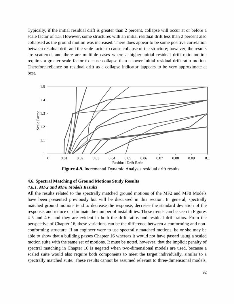
92

Typically, if the initial residual drift is greater than 2 percent, collapse will occur at or before a

scale factor of 1.5. However, some structures with an initial residual drift less than 2 percent also

collapsed as the ground motion was increased. There does appear to be some positive correlation

between residual drift and the scale factor to cause collapse of the structure; however, the results

are scattered, and there are multiple cases where a higher initial residual drift ratio motion

requires a greater scale factor to cause collapse than a lower initial residual drift ratio motion.

Therefore reliance on residual drift as a collapse indicator ]appears to be very approximate at

best.

Figure 4-9. Incremental Dynamic Analysis residual drift results

4.6. Spectral Matching of Ground Motions Study Results


All the results related to the spectrally matched ground motions of the MF2 and MF8 Models

have been presented previously but will be discussed in this section. In general, spectrally

matched ground motions tend to decrease the response, decrease the standard deviation of the

response, and reduce or eliminate the number of instabilities. These trends can be seen in Figures

4-5 and 4-6, and they are evident in both the drift ratios and residual drift ratios. From the

perspective of Chapter 16, these variations can be the difference between a conforming and non-

conforming structure. If an engineer were to use spectrally matched motions, he or she may be

able to show that a building passes Chapter 16 whereas it would not have passed using a scaled

motion suite with the same set of motions. It must be noted, however, that the implicit penalty of

spectral matching in Chapter 16 is negated when two-dimensional models are used, because a

scaled suite would also require both components to meet the target individually, similar to a

spectrally matched suite. These results cannot be assumed relevant to three-dimensional models,

1

1.1

1.2

1.3

1.4

1.5

0 0.01 0.02 0.03 0.04 0.05 0.06 0.07 0.08 0.09 0.1

Sca

le F

acto

r

Residual Drift Ratio

93

since the implicit penalty will be included, as the scaling requirements differ between amplitude

scaled and spectrally matched ground motions for three-dimensional models.


In contrast with the MF2 and MF8 Models, the comparison between scaled and spectrally

matched suites for the 3D Model indicated that the spectrally matched motions did not always

reduce the suite mean drift ratio. It is postulated that this results from the directionality of ground

motions in near-fault sites. Typically, the fault normal component of ground motion exceeds the

fault parallel for near-fault sites. This is shown for the 3D Model in Figure 4-10, where the fault

normal suite mean exceeds the fault parallel for nearly all periods of interest. When the Chapter

16 procedures for spectral matching are employed, namely matching each component rather than

the maximum direction to the target, the scale factor in the fault parallel direction is increased

more than the scale factor in the fault normal direction. Since neither the MF2 nor the MF8

Model is near-fault and since both are analyzed only in 2D, this issue does not appear in their

results.

Figure 4-10. Ratio of fault normal (left) and fault parallel (right) versus maximum direction

spectral acceleration for SCAL suite

Figure 4-7 shows that the SCAL suite mean drift ratio generally slightly exceeds the MTCH suite

mean for the SMRF (fault-normal) direction. In the BRBF (fault-parallel) direction, the opposite

is true. This is consistent with the previously described expected result given the Chapter 16

spectral matching provisions for near-fault sites. Although it was the intention that spectral

matching would receive a de facto penalty under the Chapter 16 provisions, it is evident that in

near-fault sites this may not occur when the suite mean maximum direction spectrum of the

scaled motions exceeds the target in the period range of interest. Also of interest is that spectral

0

0.1

0.2

0.3

0.4

0.5

0.6

0.7

0.8

0.9

1

0 1 2 3 4

Sa F

N/S

a RotD

100

Period [s]

Individual Records

Suite Mean

0

0.1

0.2

0.3

0.4

0.5

0.6

0.7

0.8

0.9

1

0 1 2 3 4

Sa F

P/S

a Ro

tD1

00

Period [s]

94

matching is often believed to reduce the dispersion in building response within a record suite as

compared to one that is only scaled to a target. While this holds true for the SMRF direction, the

MTCH suite in the BRBF direction exhibits a greater standard deviation than its corresponding

SCAL suite. It is possible, however, that this is more a product of the structural system

responding at higher drift ratios than a reflection on the ground motions.

4.7. Accidental Torsion Study Results

Accidental torsion is typically only included in elastic procedures, such as those that exist in

ASCE 7 Chapter 12 (ASCE 2010) and ASCE 41 (ASCE 2006 and 2013), which require that four

different locations of the center of mass be considered. These four locations are computed by

shifting the center of mass 5 percent of the diaphragm dimension in a specific direction at all

floors simultaneously. In order to assess the applicability of a nonlinear accidental torsion

requirement, these elastic procedures are expanded to inelastic analyses. The 3D Model was

analyzed using the SCAL suite of ground motions with four shifts of the center of mass,

corresponding to five total cases after including the expected center of mass location. The four

cases are listed as 5% East, 5% West, 5% North, 5% South and None in Figure 11. It should be

noted that the 3D Model was determined to meet the elastic requirements of ASCE 7 Chapter 12

(ASCE 2010) as a torsionally regular structure. The maximum ratio of δmax to δaverage is very

close to 1.0 in the SMRF direction and just less than 1.2 in the BRBF direction, which are both

less than the limiting ratio of 1.2 for a torsionally irregular structure. To catch the full effect of

the accidental torsion, the displacements are checked at the corners of the lateral system. All

results previously reported in this work were at the expected center of mass location. The

maximum corner drifts are averaged over the ground motion suite at each story.

The diaphragm geometry has a rather high aspect ratio with the dimension in the East-West far

exceeding that in the North-South direction. Resulting from this, the 5 percent rule produces a

greater shift in the East-West direction and therefore a larger change in the BRBF corner story

drift ratios as seen in Figure 4-11. In this direction, the corner drifts increase as much as 25

percent when accidental torsion is added. As expected, the 5 percent East and 5 percent West

locations of the center of mass produce the largest corner drifts in this direction. Note that results

in the SMRF direction are nearly identical for all locations of the center of mass due to the small

shift produced by the 5 percent rule. Note that to avoid biasing the mean, one ground motion that

was shown to produce drifts well above the rest of the suite was eliminated for this accidental

torsion study.

95

Figure 4-11. Mean corner story drift ratios for each mass eccentricity location of the 3D Model

for SMRF (left) and BRBF (right) direction

4.8. Implicit Satisfaction of Collapse Probability Results


The standard P-695 methodology to compute the probability of collapse is implemented for the

MF2 and MF8 Models without the inclusion of the gravity system (as prescribed by the standard

methodology). The MF2 and MF8 Models are analyzed as Risk Category II structures, and

therefore, must have a probability of collapse less than or equal to 10 percent under the MCER

level ground motion. Using the 44 far-field ground motions scaled to the design spectrum,

incremental dynamic analysis is performed until 22 ground motions cause collapse. For the MF2

Model, the probability of collapse is 1.08 percent, and for the MF8 Model, the probability of

collapse is 4.68 percent. Both of these models have a probability of collapse below 10 percent.

Even though the MF8 Model did not satisfy the Chapter 16 drift requirements, it did satisfy the

P-695 requirements. It is important to note that any analysis that creates an instability or non-

convergence is deemed immediately unacceptable by Chapter 16 standards, which may not

necessarily equal a total collapse. The P-695 procedure, on the other hand, only stops an analysis

when a full collapse of the structure has occurred.

0

1

2

3

4

5

6

0 0.02 0.04 0.06 0.08 0.1

Sto

ry

SMRF Stroy Drift Ratio

None - Mean

5% East - Mean

5% West - Mean

5% North - Mean

5% South - Mean

0

1

2

3

4

5

6

0 0.01 0.02 0.03

Sto

ry

BRBF Stroy Drift Ratio

96


Appendix F is used for the analysis of the 3D Model, as it is prescribed for individual structures.

For this methodology, one single scale factor is determined for each direction, which is based on

the acceptable probability of collapse (FEMA 2009a). The 3D Model is Risk Category III, and

therefore, must have a probability of collapse less than or equal to 6 percent under the MCER

level ground motion. These scale factors are determined as 3.41 in the SMRF direction and 3.13

in the BRBF direction. The suite of 56 normalized near-fault ground motions is then scaled by

these factors, and nonlinear response history analyses are run for each motion. If fewer than 28

of the ground motions cause collapse, the building performance is acceptable. A non-simulated

collapse limit is chosen for the drift ratios as 10 percent, and if any drift ratios exceed this limit,

the building will be considered to have collapsed. This value was chosen because it was

previously used in ATC 76 for BRB Frames (NIST 2011), and the IDA curves for the moment

frame systems of the MF2 and MF8 Models also tend to flatten near this limit during the

incremental dynamic analyses discussed previously.

For the 3D Model, 33 ground motions caused collapse, which implies that the probability of

collapse is greater than the maximum acceptable value of 6 percent. An exact probability of

collapse cannot be calculated, because IDA is not performed. It is important to note that specific

modeling choices (such as including the inclusion of the lateral resistance of the gravity system)

could dramatically change the outcome for this structure. Additionally, there is subjectivity in the

dispersion selections in the P-695 procedure, which will affect the results. Sensitivity to such

variables was not undertaken for the 3D Model.


For both MF2 and MF8 Models, the systems are analyzed with and without the lateral strength

and stiffness of the gravity system. In all cases, the mean response and the dispersion decrease,

as expected when more resistance is captured. Additionally, the instabilities are always

eliminated when the gravity system influence is included. For these examples, the inclusion of

the gravity system was the difference between an acceptable and an unacceptable structure with

respect to the Chapter 16 requirements. The addition always provides a relative improvement in

performance, so it is the opinion of the authors that the absence of strict requirements by Chapter

16 to include the gravity system is acceptable. If the modeler chooses to develop a more accurate

response and expects the lateral influence of the gravity system to be crucial to the overall

response of the system, this option is still available. However, it is important for the modeler to

acknowledge that the gravity system can provide a factor of safety against collapse during

earthquake events, but this factor of safety is eliminated if the gravity system’s lateral resistance

is included in the design. If the structure is acceptable without modeling the lateral resistance of

the gravity system, it would be unnecessary to include it. However, there is benefit in modeling

the gravity system to model all P-Delta effects, whether the lateral resistance is included or not.

97

There are many factors for the engineer to consider regarding the modeling of the gravity system,

which supports the lack of a stringent requirement.

In contrast to some performance-based design guidelines, Chapter 16 does not require a check of

residual drifts, instead relying on other criteria. It is shown in the studies of the MF2, MF8 and

3D Models that residual drifts can be quite high for structures conforming to Chapter 16.

However, no significant link is determined from the residual drift IDAs between the magnitude

of residual drift and the proximity to collapse, which is the same conclusion found in the

literature (Lee and Foutch 2003). Additionally, the MCER level ground motion required scaling

by at least 120 percent to reach collapse for every ground motion. This simple IDA process can

provide valuable information on the post-earthquake condition of a structure and could be added

in as commentary; however, the results of this investigation do not warrant a formal

recommendation to require a residual drift check, since ASCE 7 is first tasked with preventing

collapse.

All analyses were performed using a suite of recorded ground motions both amplitude scaled and

spectrally matched to a target spectrum per Chapter 16. For the MF2 and MF8 Models, the

spectrally matched ground motions tended to reduce the drift response and the dispersions when

compared to the response of the amplitude scaled ground motions. These analyses show that

spectral matching should not be applicable to two-dimensional models since the inherent penalty

of spectral matching is negated. This problem is eliminated with the requirement that only three-

dimensional models are acceptable. The 3D Model showed greater drifts and dispersion in the

fault parallel direction for spectrally matched versus scaled suites and vice versa in the fault

normal direction. Spectral matching in near-field sites tends to amplify fault parallel motions

more than fault normal. It can, in fact, lead to decreased response in the fault normal direction as

compared to a scaled record suite when the scaled suite’s mean maximum direction spectrum

does not perfectly match the target. Therefore, spectrally matched ground motions should be

used cautiously, if at all, for near-field sites because of the inherent directionality of ground

motions close to faults. These analyses also did not attempt to characterize the modification to

the pulse characteristics of the near-fault records as is required in Chapter 16. Further work

should be done to ensure that the spectral matching procedure is valid for three-dimensional far-

field models. The inherent penalty could also deter their use in the Chapter 16 procedure.

Chapter 16 uses a simple approach to including accidental torsion. Rather than including it in the

nonlinear response history analysis step, it simply requires that the Chapter 12 provisions (i.e.

elastic accidental torsion checks) be satisfied. This research looks at the effects of nonlinear

accidental torsion, which expands on the elastic procedure where the center of mass is shifted 5

percent of the diaphragm dimension in each direction. The analysis of the 3D Model provides

preliminary verification that accidental torsion can have a significant effect on the nonlinear

98

behavior of a structure, even for a torsionally regular building. The elastic procedures are not

comprehensive, and the issue of accidental torsion still needs more work for further versions of

Chapter 16. However, due to the limited research currently completed on nonlinear accidental

torsion, there is insufficient information to include provisions for it at this time. Additional work

providing recommendations for methods of assessing accidental torsion in future nonlinear

provisions are discussed elsewhere (Jarrett et al. 2014).

One of the major assumptions in Chapter 16 is that the methodology satisfies a specified

probability of collapse given the MCER through implicit criteria. To check this assumption, the

MF2, MF8 and 3D Models were analyzed under both the Chapter 16 provisions and by the

FEMA P-695 methodology. Even though the MF2 and MF8 Models without the gravity system

failed the Chapter 16 criteria, the probability of collapse calculated by the P-695 methodology

did not exceed the limit for Rick Category II structures of 10 percent. On the other hand, the Risk

Category III 3D Model did not satisfy the acceptable probability of collapse of 6 percent but does

satisfy the Chapter 16 requirements under some of the ground motion suites. It therefore does not

appear that the satisfaction of Chapter 16 requirements positively implies satisfaction of the

maximum probability of collapse or vice versa in all cases, especially considering the subjective

choices in modeling and the P-695 procedure.

Although the assumptions investigated could easily be expanded to any other methodology that

provides recommendations for the application of nonlinear response history, this work was

developed using a limited number of examples. The assumptions should be analyzed for

numerous different structures to determine the applicability of the results to any other structure

types and configurations.

99

Chapter 5: “Accidental Torsion in Nonlinear Response History Analysis”

Jordan A. Jarrett, Reid B. Zimmerman, Finley A. Charney

[Submitted to Tenth U.S. National Conference on Earthquake Engineering]

Abstract

Accidental torsion is not required in most of the recommended provisions for nonlinear response

history analyses (NRHA), including those of FEMA P-695, FEMA P-58, and the PEER Tall

Building Initiative. Linear procedures for assessing accidental torsion exist in ASCE 7 Chapter

12 and ASCE 41 Chapter 3 where the center of mass is shifted 5 percent of the diaphragm

dimension in each direction independently. However, studies have shown that accidental torsion

can have a significant effect on the inelastic behavior of structures, and the traditional elastic

methods of assessing accidental torsion may not sufficiently capture the potential inelastic

torsion behavior. These effects can be especially important for structures with minimal inherent

elastic torsion. This research uses a torsionally-regular five-story steel structure to investigate the

effects of accidental torsion in NRHA. Several methods to assess accidental torsion are

considered in the research, one of which is to apply the linear procedures that shift the center of

mass by 5 percent of each diaphragm dimension to NRHA. Accidental torsion from random

modifications in strength and stiffness are also investigated. These analyses show that accidental

torsion can have a significant effect on the inelastic behavior of this structure, particularly for

shifts in mass; therefore, the inclusion of accidental torsion within provisions for NRHA is

warranted. However, the four shifts in mass significantly increase the computational demand, so

this work also investigates ways to minimize the required number of shifts by using either the

calculated location of the center of rigidity or nonlinear pushover analyses. This paper provides

suggested code language for a NRHA provision that includes an exception to reduce the number

of mass shifts, as applicable.

5.1. Introduction

Under seismic loads, structures can be subjected to effects from two types of torsional

influences: inherent torsion and accidental torsion. Inherent torsion includes the effects of the

difference in location of the center of rigidity from the center of mass, while accidental torsion

includes unaccounted effects from phenomena such as non-uniform ground motion input,

variations in floor masses over the life of a structure, and strength and stiffness degradation

during nonlinear response of lateral force-resisting elements. Accidental torsion is generally not

included in performance-based earthquake engineering provisions, including the PEER Tall

Building Initiative (PEER 2010), the FEMA P-695 procedure (FEMA 2009), and the FEMA P-

100

58 procedure (FEMA 2012). Typically, accidental torsion is only included in elastic procedures,

such as ASCE 7 Chapter 12 (ASCE 2010) and ASCE 41 Chapter 3 (ASCE 2006), where the

center of mass is shifted by 5 percent of the diaphragm dimension in each direction

independently. The 2009 NEHRP provisions, in the resource paper on seismic response history

analysis, recommend that if accidental torsion is included in the strength design of the nonlinear

structural elements (i.e. ASCE 7 Chapter 12 requirements), it does not need to be included in the

nonlinear response history analysis (FEMA 2009c). The effect of accidental torsion is

investigated in this research to determine if there is a necessity for its inclusion within nonlinear

response history analyses (NRHA) or if the current state of provisions for NRHA is correct in

excluding it.

Studies have shown that the uncertainty in the location of the center of mass is normally the

largest influence to accidental torsion (De la Llera and Chopra 1995). This explains why the 5

percent offset procedure is typically used, since it relates to the distribution of mass on each

floor. The practical concern for response history analysis is that the four shifts in mass location

quadruples the number of analyses performed, since the structure must be analyzed with four

shifted center of mass locations, instead of the one computed center of mass location. Another

concern with this method is that while the uncertainty in the center of mass tends to contribute

the most to accidental torsion, it is not the only source of accidental torsion, particularly for

elastically torsionally-regular structures. Damage during earthquakes such as experienced by the

Clarendon Tower during the Canterbury Earthquake Sequence suggests that accidental torsion

due to asymmetric changes in strength or stiffness can be significantly important even for

structures with that are elastically torsionally-regular (Holmes and Zimmerman 2012). These

effects can be especially substantial in (originally) perfectly symmetric structures, and the

method of shifting the center of mass in the elastic analysis-based design (like those from ASCE

7 and ASCE 41) may not be sufficient to capture all the effects of accidental torsion (Dimova

and Alashki 2003). It is important to distinguish buildings based on their sensitivity to torsional

response. Some structures appear to be elastically torsionally sensitive, meaning that accidental

torsion effects cause significant changes in the torsional rotation of the building when considered

in the linear range of response. The classic case of this type of structure is one that is cruciform-

shaped in plan. Inelastically torsionally sensitive buildings, like the previously mentioned

Clarendon Tower, are those that may or may not exhibit elastic torsional sensitivity but for which

accidental torsion effects significant changes in the torsional rotation of the building when

responding in the inelastic range.

Recent research has shown that buildings designed with and without the traditional linear

accidental torsion provisions often behave similarly when experiencing inelasticity, showing a

flaw in the way accidental torsion is currently handled (Stathopoulos and Anagnostopoulos

2010). This was one of the first studies on accidental torsion that used a more realistic multi-

101

story structure to investigate torsional effects, as most of the previous studies on the topic use

single story structures or simplified shear-beam models. Their recommendation was to remove

the accidental torsion provision in its current state, except potentially for symmetric buildings.

Several additional studies have come to a similar conclusion that current code-based accidental

torsion provisions do not adequately deal with nonlinear behavior. A summary of these studies

can be found in a research review by De Stefano and Pintucchi (DeStefano and Pintucchi 2008).

While the general conclusion of these studies is that the inclusion of accidental torsion in design

is unnecessary, the results could infer that linear design provisions cannot adequately capture

inelastic torsional effects, especially for inelastically torsionally sensitive buildings, and that the

inclusion of an accidental torsion provision should be moved to the nonlinear analysis of these

structures.

This idea is reinforced in a study where the linear procedure of shifting the center of mass by 5

percent was applied to nonlinear analyses to compare the linear and inelastic responses (Mansuri

2009). That work found that the inelastic response to accidental torsion can be significantly

greater than the elastic response. This method of shifting the center of mass during nonlinear

analyses was also used to determine the effect of accidental torsion on the collapse capacity of

structures (DeBock et al. 2013). The effects of shifting the mass in elastically torsionally regular

structures had a small effect on the collapse capacity (less than 10 percent reduction), since the

collapse was controlled by lateral movements. On the other hand, shifting the mass had

significant effect on the collapse capacity of elastically torsionally irregular buildings. The work

presented in this paper will also investigate the effects of accidental torsion during NRHA, but

specifically for the maximum considered earthquake ground motion level.

5.2. Modeling Descriptions and Assumptions

To determine the accidental torsion effects in NRHA, a three-dimensional model representative

of the lateral force-resisting system (LFRS) of an actual commercial building is used. Its LFRS

consists of two lines of steel special moment-resisting frame (SMRF) in the longitudinal

direction and four lines of buckling-restrained brace frame (BRBF) in the transverse direction

over five stories. Reinforced concrete walls are located around the building perimeter at the

lowest floor. Each floor is assumed to have a rigid diaphragm, except the first floor, where the

diaphragm flexibility is explicitly modeled. The SMRFs align with the fault normal component

of the ground motion, and the BRBFs align with the fault parallel component. The gravity

system is not included in the model, and a leaning column is provided to capture the P-Delta

effects. Foundation flexibility and soil-structure interaction were not included. It should be noted

that the structure was determined to meet the elastic requirements of ASCE 7 Chapter 12 (ASCE

2010) as an elastically torsionally regular structure, as the maximum ratio of δmax to δaverage is

1.02 in the SMRF direction and 1.18 in the BRBF direction, which are both less than the limiting

ratio of 1.2.

102

The building is modeled in Perform 3D (CSI 2011), and all crucial nonlinear behavior is

incorporated, including localized axial-moment-moment (PMM) interacting hinges for SMRF and

BRBF columns, moment-rotation hinges for SMRF beam-column connections and BRBF beams

outside of gusset plates, buckling-restrained brace (BRB) elements, and shear stress-shear strain

material models for concrete walls. More detail on this structure and the modeling assumptions

can be found elsewhere (Zimmerman et al. 2013). A plan view of the lateral force-resisting

elements in the structure can be found in Figure 5-1, including the locations of the center of mass

(COM) and center of rigidity (COR), each averaged over all the stories. It is important to note that

the location of these points is based on the entire structure, not just the elements shown in Figure 5-

1.

Figure 5-1. Schematic of the lateral force-resisting system of the example building

A target response spectrum for the maximum considered earthquake (MCER) is developed for

the near-fault site of the structure in Berkeley, California. Due to the proximity to the Hayward

Fault, the target spectrum is deterministically capped by the 80 percent lower limit of ASCE 7

Section 21.3 (ASCE 2010). A suite of eleven record sets are selected to match the tectonic

setting, magnitude, distance and near-fault effects controlling the seismic hazard at the site. The

horizontal ground motion components of a record set are used to construct a maximum direction

spectrum. The maximum direction spectra are scaled such that the mean over the suite fits the

target spectrum on average and does not fall below 0.9 times the ordinate of the target spectrum

in the period range of interest. More detail about the design spectrum and the ground motion

selection and scaling can be found elsewhere (Zimmerman et al. 2013). Note that the suite

average maximum direction spectrum exceeds the target spectrum in the 1.0 to 2.5 sec period

range due to near-fault effects which are included in the selected ground motions but are not

reflected in the target spectrum. Figure 5-2 shows the maximum direction spectra of the scaled

suite versus the target spectrum.

B

RB

F

B

RB

F

B

RB

F

SMRF

SMRF B

RB

F

Average COR

Average COM

103

Figure 5-2. Maximum direction spectra versus the target spectrum for the suite of ground

motions

In order to determine the effects of accidental torsion on the response during NRHA, accidental

torsion is modeled in a variety of ways. Initially, the response from accidental torsion is modeled

using the traditional method of shifting the center of mass. The effects of random strength and

stiffness degradation are also investigated. The procedure and results of these various

investigations are discussed next.

5.3. Accidental Torsion Modeled with Shifts in the Center of Mass

To investigate the effects of accidental torsion from shifts in the center of mass, eight shifts are

investigated, corresponding to nine total cases including the expected center of mass location

(the unaltered model). To see the most extreme effect that the torsion has on the structure, it is

important to look at the displacements at the corners of the building, which are shown in Figure

5-3 for the nine cases. The eight shifts can be broken into two groups: the four traditional mass

offset cases and four diagonal mass offsets. The traditional cases correspond to the following

eccentricities (relative to the total building dimension in the same direction): 5% East, 5% West,

5% North, and 5% South. The diagonal mass offsets are defined as Northeast, Southeast,

Southwest and Northwest, where there is a 5 percent eccentricity in each of the two orthogonal

directions simultaneously. For example, the Northwest eccentricity has a 5 percent eccentricity in

the north direction plus a 5 percent eccentricity in the west direction. Relative to the non-

diagonal shifts, the 5 percent diagonal shifts may be too conservative, but these preliminary

results will provide trends between different potential mass locations. The diaphragm geometry

has a rather high aspect ratio, with the dimension in the East-West far exceeding that in the

North-South direction. Resulting from this, the 5 percent mass offset produces a greater shift in

the North-South (BRBF) direction, and the effects in the East-West (SMRF) direction are

0

0.5

1

1.5

2

2.5

3

0 0.5 1 1.5 2 2.5 3 3.5 4

Sp

ectr

al a

ccel

erat

ion

[g]

Period [s]

Average


Target spectrum


104

negligible due to the small diaphragm dimension. Therefore, only the drifts in the BRBF

direction are presented in Figure 5-3, which shows the maximum of the four average corner drift

ratios along the height of the structure.

Figure 5-3. Corner story drift ratios computed by first averaging over all ground motions within

a suite and then maximizing over each corner in the BRBF direction only

In the BRBF direction, these mean drift ratios can increase by up to 25 percent when the 5

percent eccentricities are included. Additionally, two of the diagonal mass offsets tend to

envelope the four “traditional” mass offsets, which in this case are the southeast and northwest

mass offsets. Since running multiple mass offsets is computationally demanding, two procedures

to determine the most crucial mass offsets are discussed in the next two sections.

5.3.1. Determine Which Traditional Eccentricities to Evaluate Using Pushover Data

Nonlinear pushover analysis is a method of analysis that is significantly less computationally

demanding than nonlinear dynamic analyses, and it is often used to check a mathematical model

for errors and to determine the distribution of inelasticity. In this procedure, nonlinear pushover

analyses are additionally used to determine which traditional mass offset(s) should be analyzed

using NRHA and which can be ignored. Nonlinear pushovers were performed in the North

direction and the East direction at the true center of mass and at each traditional shift in the

center of mass location, using the exact same mathematical model used in the dynamic analyses.

Figure 5-4 shows the results from the pushover analyses in the North direction where there is a 5

percent eccentricity in the West or East direction. These figures plot the base shear against the

0

1

2

3

4

5

0 0.005 0.01 0.015 0.02 0.025 0.03 0.035

Sto

ry

Maximum Mean Corner Drift Ratios

Unaltered ModelNorthEastSouthWestNortheastSoutheastSouthwestNorthwest

105

roof drift ratio in the North direction at three locations: the approximate center of the building

(Roof Y), the northeast corner (Roof NE Y) and the northwest corner (Roof NW Y). Due to the

small dimension of the structure in the North-South direction, the torsional influences from the

pushovers in the East direction are negligible and not shown.

Figure 5-4. Pushover curves in the North direction where there is a 5% eccentricity to the West

(left) and 5% eccentricity to the East (right)

When the pushover is performed at the West eccentricity, there is a 34 percent difference

between the largest corner drift and the center drift at the end of the analysis. When the pushover

is performed at the East eccentricity, there is a 44 percent difference between the largest corner

drift and the center drift at the end of the analysis. These pushover results suggest that there

could be a significant effect from accidental torsion on this structure in the nonlinear range of

response, even though little is predicted for the linear range of response (recall that the structure

was torsionally regular). Using the results of these pushover curves, a method to determine the

necessary mass offsets could be developed. For example, the dynamic analysis associated with a

given mass offset need not be performed if it is shown by nonlinear static pushover analysis

using the same mass offset that the maximum corner displacement of every level is less than 1.2

times the average displacement at that same level. Figure 5-5 shows these ratios of maximum

corner displacement to the displacement at the COM at the target drift for the pushovers in both

the North and East direction.

For this example, the target displacement used in the pushover analysis is equal to 3 percent of

the roof height, computed at the center of mass. The lateral load pattern for the pushover analysis

is proportional to the first mode shape in the direction of interest. Based on these results, the only

accidental torsion mass offsets that would be required for this structure under the above method

would be the 5 percent eccentricity in the East and West directions. As was shown in Figure 5-3,

the East and West eccentricity did in fact have the highest influence on the response history drift

0

1000

2000

3000

4000

5000

6000

0 0.01 0.02 0.03 0.04 0.05

Bas

e S

hea

r (k

)

Drift Ratio

Roof Y

Roof NE Y

Roof NW Y

0

1000

2000

3000

4000

5000

6000

0 0.01 0.02 0.03 0.04 0.05

Bas

e S

hea

r (k

) Drift Ratio

106

results (with the East eccentricity controlling for the upper stories and the West one controlling

for the lower stories). With this method, the computational demand is significantly reduced,

since only two mass offsets are required, as opposed to the traditional four.

Figure 5-5. Ratio of maximum corner drift to center of mass drift at a COM drift ratio of 3% due

to a pushover in the East direction (left) and North direction (right)

5.3.2. Alternative Method for Assessing Accidental Torsion

As Figure 5-3 shows, there were two diagonal mass offsets that encompass all the traditional

accidental torsion mass offsets. Assuming these diagonal mass offsets could be predicted,

another method to assess accidental torsion influence would be just to run the two enveloping,

diagonal mass offsets. The following procedure provides a method to determine these worst mass

offsets. By calculating the true center of rigidity, the worst case scenario eccentricities could be

determined as the diagonal in the quadrant near and opposite to the center of rigidity. The center

of rigidity for this example is determined with the method used by ETABS (CSI 2012). For

every story in this structure, the true center of rigidity is located in the northwest quadrant, and

the average distance between the COM and the COR is (-20.3, 92) inches or (-0.7% X, 12.8%

Y). This equates to an angle of 77.6 degrees clockwise from the West axis. This location of the

center of rigidity would predict that the northwest and southeast diagonals would be worst case

scenarios. This matches the results shown in Figure 5-3, where the two diagonal mass offsets that

envelope the four “traditional” mass offsets are the southeast and northwest mass offsets.

Using the diagonal mass offsets with a 5 percent offset in each direction would still be an

approximate solution, since the angle to the true location of the center of rigidity will differ from

the angle to this approximate diagonal. To determine this effect, the NRHA is performed at mass

locations with two different angles: at the “approximate angle” of 45 degrees and at the “true

0

1

2

3

4

5

1 1.05 1.1 1.15 1.2

Sto

ry

Ratio

North Ecc.

South Ecc.

0

1

2

3

4

5

1 1.2 1.4 1.6 1.8

Sto

ry

Ratio

East Ecc.

West Ecc.

107

angle” of 78 degrees clockwise from the West axes. The length of these offsets is held constant

as the length determined from the approximate location. Figure 5-6 shows the maximum of the

mean corner drift results of the response history analyses with no mass offset (Unaltered Model),

at the enveloping “diagonal” mass offsets (Southeast and Northwest), and at the new mass

offsets based on angle of the center of rigidity (Away from COR and Towards COR). The mass

offset based on the center of rigidity provides similar results to those from the enveloping

diagonal mass offset, particularly in the controlling quadrant, which is opposite to the center of

rigidity. It appears, at least for this structure, that using just the approximate diagonal shift

located in the quadrant opposite to the center of rigidity would sufficiently (and conservatively)

predict the maximum response from the accidental torsion. Instead of four accidental torsion

mass offsets, only one or two cases are needed.

Figure 5-6. Corner story drift ratios computed by first averaging over all ground motions within

a suite and then maximizing over each corner in the BRBF direction only

5.4. Accidental Torsion Modeled with Random Strength and Stiffness Degradation

One concern about the traditional methods of analyzing accidental torsion by shifting mass

locations is that it can only indirectly capture the torsional response from changes in strength and

stiffness. As discussed before, this source is often negligible but occasionally can produce

significant effects. This section investigates another approach to assessing torsional sensitivity

through explicit modification of individual component strength and stiffness. Twelve different

0

1

2

3

4

5

0 0.005 0.01 0.015 0.02 0.025

Sto

ry

Maximum Mean Story Drift Ratios

Unaltered Model

Southeast

Northwest

Away from COR

Towards COR

108

analyses were run with varying random reductions in stiffness and strength. Ten of these

analyses reduce the strength or stiffness of five to ten randomly selected moment frame beams or

buckling restrained braces by 10 percent. The other two analyses reduce the strength of an entire

frame by 10 percent. Figure 5-7 compares the suite mean story drift ratio results without any

strength or stiffness reduction (Unaltered Model) to the maximum of the randomly varying

strength and stiffness analyses.

There is minimal effect on this structure under random decreases in strength and stiffness. The

mean change in response under the scenarios where 5 to 10 members have strength or stiffness

reduction is less than 1 percent. Even when the strength of an entire BRB frame is reduced by 10

percent and the reduction is limited to one side of the structure, the maximum increase in mean

drift ratio is 6.5 percent, as the results in Figure 5-7 show. This procedure provides minimal

insight into the behavior of this structure when compared to the method of moving the center of

mass. However, this effect may have more influence on other structures, and the procedure could

be useful to check if a particular structure is susceptible to this influence.

Figure 5-7. Comparison of the suite mean story drift ratio results without any strength or

stiffness reduction (Unaltered Model) to the maximum of the randomly varying strength and

stiffness analyses in the SMRF direction (left) and the BRBF direction (right)

5.5. Conclusions

This work demonstrates that accidental torsion can have a significant impact on the nonlinear

behavior of a structure and that shifting the location of the center of mass has a greater influence

than random variation in strength and stiffness for this example. This work also shows that it is

possible to predict the worst cases for the location of the shifted center of mass using nonlinear

pushover analysis. The authors believe that accidental torsion should be included in provisions

109

for nonlinear response history analyses, even for structures that are elastically torsionally regular,

and example code language is shown next in italics. This example code language is based on an

introductory set of analyses, and more examples and engineering expertise should be used to

finalize the values underlined (e.g. 5 percent) of this language.

The analysis shall consider the effect of both inherent and accidental torsion. Accidental torsion

shall be included by displacing the center of mass each way (i.e. plus or minus) from its expected

location by a distance equal to 5 percent of the horizontal dimension of the structure at the given

floor measured parallel to the direction of mass offset. The required 5 percent displacement of

the center of mass need not be applied in both orthogonal directions at the same time.

Exception: The dynamic analysis associated with a given center of mass offset shall not

be required if the following is satisfied: It is shown by nonlinear static pushover analysis,

using the same mass offset, that the maximum corner drift is less than 1.2 times the

average drift at all levels of the structure. The roof target drift used in the nonlinear

static analysis shall be equal to the maximum roof drift ratio permitted for the structure,

and the lateral load pattern for the pushover analysis shall be proportional to the first

mode shape in the direction of interest.

Numerous previous works have highlighted the potential flaws of including the accidental

torsion only in the design and linear analyses of the structure, and this work highlights the need

for the inclusion of accidental torsion in nonlinear analyses. Assuming a structure barely satisfies

the drift limits of a provision for NRHA without accidental torsion, the drifts including the

nonlinear effects of accidental torsion could be dangerously large and unaccounted for. The

addition of code language similar to the above would ensure the inclusion of accidental torsion in

the NRHA of structures that are strongly influenced by its effect, while reducing the

computational demand for structures where accidental torsion is not as critical.

110

6. Summary, Conclusions and Future Work

The performance assessment of seismic resistant structures is a broad research topic with many

interesting facets. This work investigates a few topics related to this performance assessment,

stemming from two different studies. The first study compared the performance of newly

developed and traditional seismic resisting systems, and the second study investigated many of

the assumptions made within provisions for nonlinear response history analyses.

This final chapter provides a summary of work contained in this dissertation. The first section

provides an overview of the work and a summary of the results. The second section discusses the

potential future work.


6.1.1. Comparison of Methodologies

Preliminarily, this work focused on the comparison of various methods available for the

performance assessment of seismic resistant structures. In the two studies presented in the

manuscripts, three methodologies were used extensively: FEMA P-695, FEMA P-58, and the

proposed updates to ASCE 7 Chapter 16. This section will summarize the comparison of these

methodologies, particularly the advantages and disadvantages.

From a modeling standpoint, all these methodologies have very similar requirements. While

some of the specific details vary, all the methodologies require a model that captures all the

hysteretic behavior and nonlinearities of the elements. There are some differences (notably the

inclusion of the gravity system resistance, force-controlled versus deformation-controlled

elements, and the allowance of two-dimensional analysis), but the overall idea of creating a

model that captures the true behavior of the structure as much as possible is the same throughout

all the nonlinear analysis methodologies. The major differences between the methodologies are

the evaluated limit states, the computational demand, the post processing of the results and the

major outputs.

The ASCE 7 methodology is the most common methodology and the one referenced in coded

design. Out of the three methodologies, it is the most simplistic method and requires the least

amount of computational effort. However, from a performance based earthquake engineering

standpoint, it is not an effective methodology. It only looks at one limit state, and once the

demands (drifts and forces) are determined, no further post-processing is prescribed, and the

output is left in terms that are not typically meaningful for stakeholders. It attempts to implicitly

satisfy a probability of collapse limit, but this is not directly calculated as it is the P-695 process.

111

The P-695 methodology, on the other hand, is the most computational demanding methodology

of the three. Hundreds, if not thousands, of nonlinear dynamic analyses must be run; a

computational demand beyond the capabilities of most practicing engineers and likely even some

academics. Just like ASCE 7, the methodology description only looks at one limit state, which in

this case, is collapse. However, the incremental dynamic analyses provide valuable information

that could be used to look at behavior at multiple levels of ground motion and fulfill the

principles of PBEE.

The P-58 methodology shows the most promise, in this author’s opinion. For intensity based

assessments, the P-58 methodology takes about the same computational demand as the ASCE 7

method (assuming a simplified method is used for predicting collapse). If the time based

assessment is used, the computational demand increases by around a factor of 8, which is still

drastically less than the P-695 analysis. This methodology currently shows the most promise,

because it takes the general ideas behind ASCE 7 and P-695, combines them, and expands on

them. The methodology performs a limit state based analysis at one or more predetermined

levels of intensity (similarly to ASCE 7), as well as a collapse analysis (which often could be the

P-695 process). It then goes a few steps further by integrating hazard with fragility (assuming a

time based assessment is used), running Monte Carlo simulation to expand the results and

account for uncertainties (in modeling, ground motion selection and scaling, and overall building

performance), and finally puts the results in terms of consequences that are more easily

understood by decision makers and stakeholders.

However, this method does come with some anticipated disadvantages. While a large number of

fragilities are included in the methodologies, including all the components of the building may

be difficult. If all the components are not accurately included, the consequence estimation could

be drastically wrong. The processes to add new fragilities are not simplistic and typically rely on

significant amounts of test data. However, to provide accurate consequence distributions, a

comprehensive set of fragilities must be developed for use within the PACT program.

Additionally, from the perspective of cost changes over time, updating all the costs estimation

with inflation and changes in supply and demands seems like a daunting task, and unless some

other parties takes responsibility of the program (as the developing team hopes), the program

could likely become abandoned and obsolete in a few years.

6.1.2. Summary and Conclusions from Comparative Study

The work of the first study is presented in a manuscript entitled “Comparative Evaluation of

Innovative and Traditional Steel Seismic Resisting Systems Using the FEMA P-58 Procedure,”

which is shown in Chapter 3. Three innovative systems and modeling assumptions are compared

to their traditional counterparts using a combination of the FEMA P-695 and P-58

methodologies. The three systems analyzed are: hybrid buckling restrained braces, collapse

112

prevention systems, and moment frames evaluated with and without the lateral influence of the

gravity system. The Hybrid BRBs and moment frames are analyzed at four intensity levels of

interest: serviceability, DBE, MCE and near-collapse level. The Collapse Prevention Systems are

only analyzed for a near-collapse level intensity, as they are designed specifically for life safety

in locations where that is the only crucial intensity level, like the Central and Eastern United

States. The results are presented in terms of repair costs, repair times, number of casualties, and

probability of receiving an unsafe placard, which are more meaningful to owners and other

decision makers.

The major results of this first study are as follows:

When compared to traditional BRB systems, the repair costs of the Hybrid BRBs are

reduced by up to 12 percent at lower intensity levels for short structures and up to 26

percent at higher intensities for the taller structures. Additionally, the repair time at the

serviceability level is always reduced by more than 10 percent.

In general for the Hybrid BRB, there was negligible change in the probability of

receiving an unsafe placards and the number of casualties.

The more hybridity in the BRB, the more the consequences are reduced. This trend was

similar to those found in the P-695 analyses, where the Hybrid 3 system always had the

smallest probability of collapse and residual drifts.

For the Collapse Prevention System at the near-collapse level, the average repair costs are

always decreased by 5 to 36 percent when the collapse prevention mechanism is added.

This reduction was greater for the slack cable device than the loose link device.

For the 2-story Collapse Prevention System model, the average number of casualties was

significantly decreased (nearly 33 percent) by the slack cable mechanism.

In general for the Collapse Prevention Systems, there was negligible change in the repair

time and the probability of receiving an unsafe placard.

By modeling this lateral resistance of the gravity system, the average costs can be

reduced significantly (up to 32 percent), particularly at higher intensity levels. For the 4-

story model, the number of casualties was noticeably reduced at higher intensities;

otherwise, all other consequences had negligible change.

6.1.3. Summary and Conclusions from Assumptions Study

The work of the second study on the assumptions in nonlinear response history analysis is

presented in two manuscripts entitled “Response-History Analysis for the Design of New

Buildings: A Study of Assumptions” and “Accidental Torsion in Nonlinear Response History

Analysis,” which are shown in Chapters 4 and 5, respectively. The first manuscript discusses all

the investigated assumptions with respect to the proposed updates to Chapter 16 of ASCE 7,

113

while the second manuscript focuses on one assumption, which is the use of accidental torsion in

nonlinear response history analyses.

The major results of this second study are as follows:

Modeling the gravity system’s lateral influence can have significant effect on the system

behavior, as the mean response and dispersion almost always decrease, and all

instabilities are eliminated. Since the results are conservative when the gravity system

resistance is included, its inclusion is unnecessary unless a more accurate representation

of the behavior is needed or the structure will not satisfy the requirements without its

inclusion.

No significant link between the magnitude of residual drift and the proximity to collapse

is determined from the residual drift IDAs in this work, and therefore, exclusion of a

residual drift check is acceptable when concerned with collapse prevention.

Spectrally matched ground motions tended to reduce the drift response and the

dispersions when compared to the response of the amplitude scaled ground motions for

the far field structures analyzed. However, for the near-field system, the spectral

matching can amplify the fault parallel motions more than the fault normal motions if the

pulse characteristics are altered. Spectrally matched ground motions should cautiously be

used for near-field structures, and the pulse characteristics must be retained.

Even though the Risk Category II models failed the Chapter 16 criteria, the probability of

collapse calculated by the P-695 methodology did not exceed the limit of 10 percent. On

the other hand, the Risk Category III model did not satisfy the acceptable probability of

collapse of 6 percent but does satisfy the Chapter 16 requirements under some of the

ground motion suites. Even if a structure is designed per ASCE 7, it may not have the

assumed probability of collapse under the maximum considered earthquake when

analyzed using FEMA P-695.

The effects of nonlinear accidental torsion are investigated by expanding on the elastic

procedure where the center of mass is shifted 5 percent of the diaphragm dimension in

each direction. Accidental torsion can have a significant effect on the nonlinear behavior

of a structure, even for a torsionally regular building. However, there are not sufficient

studies on nonlinear accidental torsion provisions to include them in the next Chapter 16

update.

Even though accidental torsion cannot be included in the proposed Chapter 16 updates,

the elastic procedures are not comprehensive, and the issue of accidental torsion still

needs more work for future NRHA provisions. The work in the third manuscript begins

this process.

Accidental torsion is assessed by applying the linear procedures that shift the center of

mass by 5 percent of each diaphragm dimension to NRHA and by randomly modifying

114

the strength and stiffness of lateral resisting members. These analyses show that

accidental torsion can have a significant effect on the inelastic behavior of this structure,

particularly for shifts in mass.

The four shifts in mass significantly increase the computational demand, so ways to

minimize the required number of shifts by using either the calculated location of the

center of rigidity or nonlinear pushover analyses are investigated. The pushover analyses

was determined at the best way to determine which shifts should be run, and the third

manuscripts provides suggested code language for a NRHA provision that includes an

exception to reduce the number of mass shifts, as applicable.

6.2. Future Work

This section will be discussed in two sections: short-term future work and long-term future work.

The short-term future work is directly related to expanding upon the research presented in this

dissertation. The long-term future work relates to the general comparison and discussion of

methodologies used for the performance assessment of seismic resistant structures.

6.2.1. Short-Term Future Work

In the short term, additional analyses should be performed for the first study (that compares

innovative and traditional systems), with new structural configurations to determine how the

trends expand to a wide variety of uses. Initially, the results could be expanded to all the

archetypes in the corresponding ATC 76 studies, as this research only presented a subset of the

archetypes and performance groups. The inclusion of the gravity system resistance should then

be expanded to a variety of other structural systems to see how the effect of this addition varies.

For the Hybrid BRBs, the P-58 analyses should be run with the residual drift inputs to determine

the additional decrease in consequences. Since the residual drifts were greatly decreased in the P-

695 analyses, this inclusion could decrease the consequences even further. For the Collapse

Prevention Systems, a detailed cost estimate should be performed, since the lack of seismic

detailing would likely decrease the overall costs. Using these accurate costs in the P-58 analyses

would likely show an additional decrease in consequences. Additionally, augmented systems that

combine the collapse prevention devices with dampers could improve behavior at numerous

intensity levels. These additional systems should be modeled and analyzed at all intensity levels

of interest, similarly for the other Hybrid BRBs and systems including the gravity system

resistance. All these systems could also be analyzed for a specific location using a time-based

assessment to see location specific benefits.

In the short term for the second study (about the assumptions within nonlinear response history

provisions), the work needs to be expanded to a variety of additional systems with varying

structural systems, configurations and materials. Particularly for the proposed accidental torsion

115

code language, these additional analyses should be used to finalize the recommended code

language. This study was performed on a limited number of models, and while the results

provide valuable insight into the assumptions, it is necessary to determine the applicability of the

results to any generic structures.

6.2.2. Long-Term Future Work

Numerous methodologies have been researched and discussed in this dissertation, particularly

ASCE 7, FEMA P-695, and FEMA P-58. All the methodologies have benefits and

disadvantages, which were summarized previously.

The largest conclusion that comes from this study of the various methodologies is that there is a

wide variety of ways to assess the nonlinear performance of seismic resisting systems. While

three methodologies are studied in detail in this work, numerous other provisions exist, including

the Tall Building Initiative and ASCE 41. In the best interest of the profession, these

methodologies should all be combined and standardized. However, this would require a

significant amount of collaboration around the country and a significant number of studies to

find the best, generic solution.

While this list should not be considered exhaustive, a single methodology for the performance

assessment of seismic resisting structures should include:

Assessment at numerous limits states, which can be adjusted based on the system and

system location

Minimal computational demand

Integration of hazard with fragility

Determination of consequences

Standardized acceptance criteria

Analysis of structural and non-structural components

Inclusion of all potential nonlinear behaviors

The FEMA P-58 procedure is the methodology that satisfies more of these criteria than any other

methodology. This procedure should provide the starting point for the development of a single,

standard methodology. Primarily, the fragilities need to be expanded to be more inclusive and to

ensure accurate cost estimations, and the best method for developing collapse fragility curves

should be determined, based on the best balance between accuracy and simplicity. Additionally,

the language should be adjusted to be prescriptive and include acceptance criteria. The modeling

assumptions should satisfy the conclusions provided in the study on assumptions based on the

proposed ASCE 7 updates, as they are applicable to all nonlinear response history analyses. In

order to accomplish this daunting task, a significant amount of research would be required by

116

both academics and practitioners. However, this universalization would be a valuable change to

the earthquake engineering profession and could potentially be the state of practice in a

significant number of years.

117

References

AISC (2011). Steel Construction Manual, American Institute of Steel Construction, Chicago, IL.

Akkar, S., Sucuo Lu, H., and Yakut, A. (2005). Displacement-Based Fragility Functions for

Low-and Mid-Rise Ordinary Concrete Buildings. Earthquake Spectra, 21(4) 901–927.

Al Atik, L., and Abrahamson, N. (2010). An Improved Method for Nonstationary Spectral

Matching. Earthquake Spectra 26, 601–617.

Ang, A., and Tang, W. (2007). Probability Concepts in Engineering, 2nd edition, John Wiley

and Sons, Inc., Hoboken, NJ.

Antoniou, S., and Pinho, R. (2004). Advantages and Limitations of Adaptive and Non-Adaptive

Force-Based Pushover Procedures. Journal of Earthquake Engineering, 8(4), 497–522.

ASCE (2005). Minimum Design Loads for Buildings and Other Structures. American Society of

Civil Engineers, Reston, VA.

ASCE (2006). Seismic Rehabilitation of Existing Buildings, American Society of Civil

Engineers, Reston, VA.

ASCE (2010). Minimum Design Loads for Buildings and Other Structures. American Society of

Civil Engineers, Reston, VA.

ASCE (2013). Seismic Rehabilitation of Existing Buildings. American Society of Civil

Engineers, Reston, VA.

Asgarian, B., Sadrinezhad, A., and Alanjari, P. (2010). Seismic Performance Evaluation of Steel

Moment Resisting Frames through Incremental Dynamic Analysis. Journal of Constructional

Steel Research, 66(2), 178–190.

Aslani, H., and Miranda, E. (2005). Fragility Assessment of Slab-Column Connections in

Existing Non-Ductile Reinforced Concrete Buildings. Journal of Earthquake Engineering, 9

(6), 777–804.

Atlayan, O. (2008). Effect of Viscous Fluid Dampers on Steel Moment Frame Designed for

Strength and Hybrid Steel Moment Frame Design. M.S. Thesis, Virginia Tech, Blacksburg,

VA.

Atlayan, O., and Charney, F. (2012). Hybrid Steel Frames. World Conference on Earthquake

Engineering, Lisbon, Portugal.

Atlayan, O., and Charney, F. (2013). Hybrid Buckling-Restrained Braced Frames. Unpublished

Manuscript.

Ayoub, A., Mijo, C. and Chenouda, M. (2004). Seismic Fragility Analysis of Degrading

Structural Systems. 13th World Conference on Earthquake Engineering, Vancouver, B.C.,

Canada, Paper 2617.

Badillo-Almaraz, H., Whittaker, A., and Reinhorn, A. (2007). Seismic Fragility of Suspended

Ceiling Systems. Earthquake Spectra, 23(1), 21–40.

118

Bazzurro, P., Cornell, C., Menun, C., and Motahari, M. (2004). Guidelines for Seismic

Assessment of Damaged Buildings, in Proceedings, 13th World Conference on Earthquake

Engineering, Paper 1708, Vancouver, Canada.

Bazzurro, P. and Luco, N. (2006). Do Scaled and Spectrum-matched Near-Source Records

Produce Biased Nonlinear Structural Responses? in Proceedings, 8th US National

Conference on Earthquake Engineering, San Francisco, CA.

Behnamfar, F., and Haghollahi, S. (2012). Collapse Performance Evaluation of Reinforced

Concrete Special Moment Frame Systems Special Moment Frame Systems Considering

Soil–Structure Interaction. 15th World Conference on Earthquake Engineering, Lisbon,

Portugal.

Bhuiyan, A., Alam, R., and Haque, N. (2012). Seismic Performance Assessment of a Continuous

Highway Bridge Seismically Isolated by Lead Rubber Bearings. Asian Transaction on

Engineering, 02(03), 62–71.

Bozorgnia, Y., and Bertero, V. (2004). Earthquake Engineering: From Engineering Seismology

to Performance-Based Engineering, CRC Press.

Charney, F., and Marshall, J. (2006). A Comparison of the Krawinkler and Scissors Models for

Including Beam-Column Joint Deformations in the Analysis of Moment-Resisting Steel

Frames. Engineering Journal – American Institute of Steel Construction 43, 31–48.

Charney, F. A., Darling, S., and Eatherton, M. R. (2012). Seismic Performance of Very Short

Period Buildings. 15th World Conference on Earthquake Engineering, Lisbon, Portugal.

Chen, C. H., and Mahin, S. (2010). Seismic Collapse Performance of Concentrically Steel

Braced Frames. Structures Congress and 19th Analysis and Computation Specialty

Conference, Orlando, Florida.

Christovasilis, I., Filiatrault, A., Constantinou, M., and Wanitkorkul, A. (2009). Incremental

Dynamic Analysis of Woodframe Buildings. Earthquake Engineering and Structural

Dynamics, 38(4), 477–496.

Cimellaro, G., and Roh, H. (2010). Fragility Analysis of Structures with Controlled Rocking

Beamcolumn Connections and Viscous Dampers. 9th U.S. National and 10th Canadian

Conference on Earthquake Engineering, Toronto, Ontario, Canada, Paper No 346.

Coffin L. F. (1954). A Study of the Effects of Cyclic Thermal Stresses on a Ductile Metal. trans.

ASME 76, 931–950.

Comeau, G., Velchev, K., and Rogers, C. A. (2010). Development of Seismic Force

Modification Factors for Cold-Formed Steel Strap Braced Walls. Canadian Journal of Civil

Engineering, 37(2), 236–249.

Computers and Structures Inc. (CSI) (2011). Nonlinear Analysis and Performance Assessment

for 3D Structures, PERFORM 3D User Guide, Berkeley, California.

Computers and Structures Inc. (CSI) (2012) Knowledge Base: Modeling Techniques, Center of

Rigidity, Berkeley, CA.

119

Constantinou, M., Tsopelas, P., Hammel, W., and Sigaher, A. (2001). Toggle-brace-damper

Seismic Energy Dissipation Systems. Journal of Structural Engineering, 127(2), 105–112.

Cundumi, O., and Laboy, S. (2010). Fragility Curves for Concrete Frame Buildings with Passive

Controllers. 9th U.S. National and 10th Canadian Conference on Earthquake Engineering,

Toronto, Ontario, Canada, Paper No 1725.

DeBock, D. J., Liel, A. B., Haselton, C. B., Hooper, J. D., and Henige, R. A. (2013). Importance

of Seismic Design Accidental Torsion Requirements for Building Collapse Capacity.

Earthquake Engineering & Structural Dynamics.

Deierlein, G., Krawinkler, H., and Cornell, C. (2003). A Framework for Performance-Based

Earthquake Engineering. Pacific Conference on Earthquake Engineering, 1–8.

Deierlein, G., Reinhorn, A., and Willford, M. (2010). Nonlinear Structural Analysis for Seismic

Design. NEHRP Seismic Design Technical Brief No. 4, NIST GCR 10-917-5, National

Institute of Standards and Technology, Gaithersburg, MD.

De la Llera, J. C., & Chopra, A. K. (1994a). Evaluation of Code Accidental-torsion Provisions

from Building Records. Journal of Structural Engineering, 120(2), 597–616.

De la Llera, J. C., & Chopra, A. K. (1994b). Accidental Torsion in Buildings. 6th

U.S. National

Conference in Earthquake Engineering, 401–410.

De la Llera, J. C., & Chopra, A. K. (1994c). Accidental Torsion in Buildings Due to Stiffness

Uncertainty. Earthquake Engineering and Structural Dynamics, 23(2), 117–136.

De la Llera, J. C., & Chopra, A. K. (1994d). Accidental Torsion in Buildings Due to Base

Rotational Excitation. Earthquake Engineering and Structural Dynamics, 23(9), 1003–1021.

De la Llera, J. C., and Chopra, A. K. (1995). Estimation of Accidental Torsion Effects for

Seismic Design of Buildings. Journal of Structural Engineering, 121, 102–114.

De Stefano, M., and Pintucchi, B. (2008). A Review of Research on Seismic Behaviour of

Irregular Building Structures Since 2002. Bulletin of Earthquake Engineering, 6(2), 285–308.

Dhakal, R., Mander, J., and Mashiko, N. (2006). Identification of Critical Ground Motions for

Seismic Performance Assessment of Structures. Earthquake Engineering & Structural

Dynamics, 35(8), 989–1008.

Dimova, S. L., and Alashki, I. (2003). Seismic Design of Symmetric Structures for Accidental

Torsion. Bulletin of Earthquake Engineering, 1(2), 303–320.

Dimova, S., and Elenas, A. (2002). Seismic Intensity Parameters for Fragility Analysis of

Structures with Energy Dissipating Devices. Structural Safety, 24 (1), 1–28.

Dolsek, M. (2009). Incremental Dynamic Analysis with Consideration of Modeling

Uncertainties. Earthquake Engineering and Structural Dynamics, 38(6), 805–825.

Ellingwood, B., Rosowsky, D., Li, Y., and Kim, J. (2004). Fragility Assessment of Light-Frame

Wood Construction Subjected to Wind and Earthquake Hazards. Journal of Structural

Engineering, 130(12), 1921–1930.

Ellingwood, B. R., and Kinali, K. (2009). Quantifying and Communicating Uncertainty in

Seismic Risk Assessment. Structural Safety, 31 (2), 179–187.

120

Elnashai, A. (2002). Do We Really Need Inelastic Dynamic Analysis? Journal of Earthquake

Engineering, 6(spec01), 123–130.

Engineering News Record (ENR) (2011). Square Foot Costbook. Design and Construction

Resources, Vista, CA.

Estekanchi, H., Vafai, A., and Sadeghazar, M. (2004). Endurance Time Method for Seismic

Analysis and Design of Structures. Scientia Iranica, 11(4), 361–370.

Farahi, M., and Mofid, M. (2013). On the Quantification of Seismic Performance Factors of

Chevron Knee Bracings, in Steel Structures. Engineering Structures, 46, 155–164.

FEMA (2000). State of the Art Report on Connection Performance, FEMA-355D. Prepared by

the SAC Joint Venture for FEMA, Washington, D.C.

FEMA (2006). Next-Generation Performance-Based Seismic Design Guidelines, FEMA 445,

Federal Emergency Management Agency, Washington, D.C.

FEMA (2009a). Quantification of Building Seismic Performance Factors, FEMA P-695, Applied

Technology Council, Washington, D.C.

FEMA (2009b). Effects of Strength and Stiffness Degradation on Seismic Response, FEMA P-

440A. Prepared by Applied Technology Council (ATC) for FEMA, Washington, D.C.

FEMA (2009c). NEHRP Recommended Seismic Provisions for New Buildings and Other

Structures, FEMA P-750, Building Seismic Safety Council, Washington, DC.

FEMA (2012). Seismic Performance Assessment of Buildings, FEMA P-58, Applied Technology

Council, Washington, D.C..

Flores, F., Jarrett, J., and Charney, F. (2012). The Influence of Gravity-Only Framing on the

Performance of Steel Moment Frames. 15th World Conference on Earthquake Engineering,

Lisbon, Portugal.

Flores, F. and Charney, F. (2013). Influence of the Gravity Framing System on the Collapse

Performance of Special Steel Moment Frames. Unpublished Manuscript.

Foschaar, J. C., Baker, J. W., and Deierlein, G. G. (2012). Preliminary Assessment of Ground

Motion Duration Effects on Structural Collapse. World Conference on Earthquake


Green, T., Leon, R., and Rassati, G. (2004). Bidirectional Tests and Partially Restrained,

Composite Beam Column Connections. Journal of Structural Engineering 130, 320–327.

Gupta, A., and Krawinkler, H. (2000). Behavior of Ductile SMRFs at Various Seismic Hazard

Levels. Journal of Structural Engineering, 126(1), 98–107.

Han, S. W., and Chopra, A. K. (2006). Approximate Incremental Dynamic Analysis Using the

Modal Pushover Analysis Procedure. Earthquake Engineering and Structural Dynamics,

35(15), 1853–1873.

Han, S. W., Moon, K.-H., and Chopra, A. K. (2010). Estimation of Collapse Capacity and

Collapse Fragility Using Modal Pushover Analysis. 9th U.S. National and 10th Canadian

Conference on Earthquake Engineering, Toronto, Ontario, Canada, Paper No 909.

Hancock, J., Bommer, J. J., and Stafford, P. J. (2008). Numbers of Scaled and Matched

121

Accelerograms Required for Inelastic Dynamic Analyses, Earthquake Engineering and

Structural Dynamics 37, 1585–1607.

Haselton, C. B., Fry, A., Baker, J. W., Hamburger, R. O., Whittaker, A. S., Stewart, J. P.,

Elwood, K. J., Luco, N., Hooper, J. D., and Charney, F. A. (2013). Response-History

Analysis for the Design of New Buildings: Part I - Development of Recommendations for the

NEHRP Provisions and the ASCE/SEI 7 Standard. Unpublished manuscript.

Holmes, W. and Zimmerman, R. (2012). Seismic Performance Investigation, Clarendon Tower,

Report prepared for Canterbury Earthquakes Royal Commission by Rutherford + Chekene.

Huang, S. N., Lu, X. Z., and Ye, L. P. (2012). A Hysteretic Model of Conventional Steel Braces

and an Analysis of the Collapse Prevention Effect of Brace Strengthening. Applied

Mechanics and Materials, 174, 3–10.

Humar, J., Adams, J., Tremblay, R., Rogers, C. A., and Halchuk, S. (2010). Proposals for the

Seismic Design Provisions of the 2010 National Building Code of Canada. 9th US National

and 10th Canadian Conference on Earthquake Engineering, Toronto, Ont., Paper No. 1387.

Iervolino, I., Manfredi, G., and Cosenza, E. (2006). Ground Motion Duration Effects on

Nonlinear Seismic Response. Earthquake Engineering & Structural Dynamics, 35 (1), 21–

38.

Jarrett, J. A., Zimmerman R. B., and Charney, F. A. (2014). Accidental Torsion in Nonlinear

Response History Analysis. Unpublished manuscript.

Judd, J. and Charney, F. (2013a). Performance‐based Design in the Central and Eastern United

States. Unpublished Manuscript.

Judd, J. and Charney, F. (2013b). Seismic Collapse Prevention System. Unpublished Manuscript.

Karim, K., and Yamazaki, F. (2003). A Simplified Method of Constructing Fragility Curves for

Highway Bridges. Earthquake Engineering and Structural Dynamics, 32 (10), 1603–1626.

Kim, J., and Rosowsky, D. (2005). Fragility Analysis for Performance-Based Seismic Design of

Engineered Wood Shearwalls. Journal of Structural Engineering, 131 1764.

Korkmaz, K. (2008). Evaluation of Seismic Fragility Analyses. The 14th World Conference on

Earthquake Engineering, Beijing, China, Paper 09-01-0141.

Koutsourelakis, S., Prévost, J., and Deodatis, G. (2002). Risk Assessment of an Interacting

Structure-Soil System Due to Liquefaction. Earthquake Engineering & Structural Dynamics,

31 (4), 851–879.

Lee, K., and Foutch, D. A. (2004). Performance Evaluation of Damaged Steel Frame Buildings

Subjected to Seismic Loads. Journal of Structural Engineering 130, 588–599.

Leon, R. T. (1998). Composite Connections. Progress in Structural Engineering and Materials,

1(2), 159–169.

Liel, A., Haselton, C., and Deierlein, G. (2006). The Effectiveness of Seismic Building Code

Provisions on Reducing the Collapse Risk of Reinforced Concrete Moment Frame Buildings.

4th International Conference on Earthquake Engineering, Taipei, Taiwan.

122

Liel, A., and Tuwair, H. (2010). A Practical Approach for Assessing Structural Resistance to

Earthquake-Induced Collapse. 19th Analysis & Computation Specialty Conference, Orlando,

FL.

Lignos, D., and Krawinkler, H. (2010). Deterioration Modeling of Steel Components in Support

of Collapse Prediction of Steel Moment Frames Under Earthquake Loading. Journal of

Structural Engineering 137, 1291–1302.

Liu, J., and Astaneh-Asl, A. (2000). Cyclic Testing of Simple Connections Including Effects of

Slab. Journal of Structural Engineering, 126(1), 32–39.

Liu, J., and Astaneh-Asl, A. (2004). Moment-rotation Parameters for Composite Shear Tab

Connections. Journal of Structural Engineering, 130(9), 1371–1380.

Lowes, L., and Li, J. (2010). Fragility Functions for Concrete Moment Frames. 9th U.S. National

and 10th Canadian Conference on Earthquake Engineering, Toronto, Ontario, Canada, Paper

No 738.

Luco, N., Bazzurro, P., and Cornell, A. (2004). Dynamic Versus Static Computation of the

Residual Capacity of a Mainshock-Damaged Building to Withstand an Aftershock. 13th

World Conference on Earthquake Engineering, Vancouver, B.C., Canada.

Luco, N., Gerstenberger, M., Uma, S., Ryu, H., Liel, A., and Raghunandan, M. (2011). A

Methodology for Post-mainshock Probabilistic Assessment of Building Collapse Risk. Ninth

Pacific Conference on Earthquake Engineering Building an Earthquake-Resilient Society,

Auckland, New Zealand.

Mackie, K., and Stojadinovic, B. (2002). Relation between Probabilistic Seismic Demand

Analysis and Incremental Dynamic Analysis. 7th US National Conference on Earthquake

Engineering, 21–25.

Mackie, K., and Stojadinovic, B. (2007). R-Factor Parameterized Bridge Damage Fragility

Curves. Journal of Bridge Engineering, 12 (4), 500–510.

Malakoutian, M., Berman, J. W., Dusicka, P., and Lopes, A. (2012). Seismic Performance and

Design of Linked Column Frame System (LCF). World Conference on Earthquake


Manson, S. S. (1953). Behavior of Materials Under Conditions of Thermal Stress. TN 2933:

NACA.

Mansuri, M. (2009). Torsional Effect on the Inelastic Seismic Response of Structures.

Dissertation, University of Southern California.

Mashal, M., and Filiatrault, A. (2012). Quantification of Seismic Performance Factors for

Buildings Incorporating Three-dimensional Construction System. World Conference on

Earthquake Engineering, Lisbon, Portugal.

MathWorks (2011). Matlab [computer software - version 2011b], Natick, Massachusetts, The

MathWorks, Inc.

123

Marshall, J. D. (2008). Development, Analysis and Testing of a Hybrid Passive Control Device

for Seismic Protection of Framed Structures. Ph.D. Dissertation, Virginia Tech, Blacksburg,

VA.

McCormick, J., Aburano, H., Ikenaga, M., and Nakashima, M. (2008). Permissible Residual

Deformation Levels for Building Structures Considering Both Safety and Human Elements,

in Proceedings, 14th World Conference on Earthquake Engineering.

McGuire, R. (2004). Seismic Hazard and Risk Analysis, Earthquake Engineering Research

Institute, Oakland, CA.

McKenna, F. (2011) OpenSEES. Version 2.3.1. Pacific Earthquake Engineering Research

Center, Berkeley, CA.

Medina, R., and Krawinkler, H. (2005). Evaluation of Drift Demands for the Seismic

Performance Assessment of Frames. Journal of Structural Engineering, 131(7), 1003.

Microsoft. (2010). Microsoft Excel [computer software]. Redmond, Washington.

Miyamoto, H., Gilani, A. S. J., Wada, A., and Ariyaratana, C. (2010). Collapse Risk of Tall Steel

Moment Frame Buildings with Viscous Dampers Subjected to Large Earthquakes. The

Structural Design of Tall and Special Buildings, 19(4), 421–438.

Moschonas, I., Kappos, A., Panetsos, P., Papadopoulos, V., Makarios, T., and Thanopoulos, P.

(2009). Seismic Fragility Curves for Greek Bridges: Methodology and Case Studies. Bulletin

of Earthquake Engineering, 7(2), 439–468.

Mwafy, A., and Elnashai, A. (2001). Static Pushover Versus Dynamic Collapse Analysis of Rc

Buildings. Engineering Structures, 23(5), 407–424.

Nakashima, M., Iwai, S., Iwata, M., Takeuchi, T., Konomi, S., Akazawa, T., and Saburi, K.

(1994). Energy Dissipation Behaviour of Shear Panels Made of Low Yield Steel. Earthquake

Engineering and Structural Dynamics, 23(12), 1299–1313.

Nakazawa, T., Kishiki, S., Qu, Z., Miyoshi, A., and Wada, A. (2011). Fundamental Study on

Probabilistic Evaluation of the Ultimate State of Base Isolated Structures. Journal of

Structural and Construction Engineering, 76(662), 745–754.

Nippon Steel (2009). Steel Plates. Nippon Steel, N.S. Corporation.

NIST (2010a). Evaluation of the FEMA P-695 Methodology for Quantification of Building

Seismic Performance Factors, NIST GCR 10-917-8, NEHRP Consultants Joint Venture,

Redwood City, CA.

NIST (2010b). Applicability of Nonlinear Multiple-Degree-of-Freedom Modeling for Design,

NIST GCR 10-917-9, Redwood City, CA.

NIST (2011). Selecting and Scaling Earthquake Ground Motions for Performing Response-

History Analyses. NIST GCR 11-917-15, NEHRP, Gaithersburg, MD.

NIST (2012). Tentative Framework for Development of Advanced Seismic Design Criteria for

New Buildings. NIST GCR 12-917-20, NEHRP Consultants Joint Venture, Redwood City,

CA.

124

Oesterle, M. G. (2003). Use of Incremental Dynamic Analysis to Assess the Performance of Steel

Moment-Resisting Frames with Fluid Viscous Dampers. M.S. Thesis, Virginia Tech,

Blacksburg, VA.

PEER (2010). Guidelines for Performance-Based Seismic Design of Tall Buildings, Report No.

2010/05, Tall Building Initiative.

Peruš, I., and Fajfar, P. (2005). On the Inelastic Torsional Response of Single‐Storey Structures

Under Bi‐axial Excitation. Earthquake engineering & structural dynamics, 34(8), 931–941.

Prowell, I., Elgamal, A., Uang, C., and Jonkman, J. (2010). Estimation of Seismic Load Demand

for a Wind Turbine in the Time Domain. Report No. NREL/CP 500, 47536.

PTC (2012). Mathcad14 [computer software], Needham, MA.

Ott, R., and Longnecker, M. (2010). An Introduction to Statistical Methods and Data Analysis,

6th Edition, Brooks/Cole, Belmont, CA.

Porter, K., Kennedy, R., and Bachman, R. (2007). Creating Fragility Functions for Performance-

Based Earthquake Engineering. Earthquake Spectra, 23(2), 471–489.

Rassati, G., Leon, R., and Noe, S. (2004). Component Modelling of Partially Restrained

Composite Joints under Cyclic and Dynamic Loading. Journal of Structural Engineering

130, 342–351.

Richard, M., Albano, L., Kelly, D., and Liel, A. (2010). Case Study on the Seismic Performance

of Reinforced Concrete Intermediate Moment Frames using ACI Design Provisions.

Structures Congress, 3523–3534.

Ruiz-García, J., and Miranda, E. (2010). Probabilistic Estimation of Residual Drift Demands for

Seismic Assessment of Multi-story Framed Buildings. Engineering Structures 32, 11–20.

Rutherford + Chekene (R+C) (2011). Perform Nonlinear Component Modeling of

StarSeismicTM Powercat BRBs, Report to StarSeismic LLC.

Saeki, E., Sugisawa, M., Yamaguchi, T., and Wada, A. (1998). Mechanical Properties of Low

Yield Point Steels. Journal of Materials in Civil Engineering, 10(3), 143–152.

Saunders, R. A. (2004). Nonlinear Dynamic Analysis of Structures with Hyperelastic Devices.

M.S. Thesis, Virginia Tech, Blacksburg, VA.

Saxena, V., Deodatis, G., Shinozuka, M., and Feng, M. (2000). Development of Fragility Curves

for Multi-Span Reinforced Concrete Bridges. The International Conference on Monte Carlo

Simulation, 499–504.

Seismic Structural Design Associates Inc. (SSDA) (2001). Description and Results of SSDA

Tests No. 23, 24, 25 and 26.

Shinozuka, M., Feng, M.Q., Lee, J., and Naganuma, T. (2000). Statistical Analysis of Fragility

Curves. Journal of Engineering Mechanics, 126 (12), 1224–1231.

Shome, N., and Cornell, C. (1998). Normalization and Scaling Accelerograms for Nonlinear

Structural Analysis. Sixth U.S. National Conference on Earthquake Engineering, EERI,

Seattle, WA, 1–12.

125

Spears, P. (2004). Parameters Influencing Seismic Structural Collapse with Emphasis on

Vertical Accelerations and the Possible Related Risks for New and Existing Structures in the

Central and Eastern United States. M.S. Thesis, Virginia Tech, Blacksburg, VA.

Stathopoulos K. G. and Anagnostopoulos S. A. (2003) Inelastic Earthquake Response of Single-

story Asymmetric Buildings: An Assessment of Simplified Shear-beam Models. Earthquake

Engineering and Structural Dynamics, 32, 1813–1831.

Stathopoulos, K. G., and Anagnostopoulos, S. A. (2010). Accidental Design Eccentricity: Is it

Important for the Inelastic Response of Buildings to Strong Earthquakes? Soil Dynamics and

Earthquake Engineering, 30(9), 782–797.

Vamvatsikos, D. (2002). Seismic Performance, Capacity and Reliability of Structures as Seen

through Incremental Dynamic Analysis. Ph.D. Dissertation, Stanford University, Palo Alto,

CA.

Vamvatsikos, D., and Allin Cornell, C. (2002). Incremental Dynamic Analysis. Earthquake

Engineering and Structural Dynamics, 31(3), 491–514.

Vamvatsikos, D., and Sigalas, I. (2005). Seismic Performance Evaluation of a Horizontally

Curved Highway Bridge Using Incremental Dynamic Analysis in 3D. 4th European

workshop on the seismic behavior of irregular and complex structures.

Vamvatsikos, D., and Cornell, A. (2006). Incremental Dynamic Analysis with Two Components

of Motion for a 3D Steel Structure. 8th US National Conference on Earthquake Engineering.

van de Lindt, J. W., Rosowsky, D. V., Pang, W., and Pei, S. (2012). Performance-Based Seismic

Design of Mid-Rise Woodframe Buildings. Journal of Structural Engineering.

Villaverde, R. (2007). Methods to Assess the Seismic Collapse Capacity of Building Structures:

State of the Art. Journal of Structural Engineering, 133(1), 57.

Wen, R., Akbas, B., and Shen, J. (2013). Practical Moment–rotation Relations of Steel Shear

Tab Connections. Journal of Constructional Steel Research, 88, 296–308.

Yun, S., Hamburger, R., Cornell, C., and Foutch, D. (2002). Seismic Performance Evaluation for

Steel Moment Frames. Journal of Structural Engineering, 128(4), 534–545.

Zareian, F., and Krawinkler, H. (2007). Assessment of Probability of Collapse and Design for

Collapse Safety. Earthquake Engineering and Structural Dynamics, 36 (13), 1901–1914.

Zareian, F., and Krawinkler, H. (2010). Structural System Parameter Selection Based on

Collapse Potential of Buildings in Earthquakes. Journal of Structural Engineering, 136(8),

933–943.

Zareian, F. (2013). PACT Beta Test Example: Building A Steel Special Moment Frame Building,

Background Document FEMA P-58/BD-3.7.14. Applied Technology Council, Washington,

D.C.

Zimmerman, R. B., Baker, J., Haselton, C. B., Bono, S., Engel, A., Hooper, J., Hamburger, R.,

Celikbas, S., and Jalalian, A. (2013). Response History Analysis for the Design of New

Buildings: Part II—Example Applications to Illustrate the Recommended Methodology.

Unpublished manuscript.

126

Zsarnóczay, Á. (2012). Influence of Plastic Mechanism Development on the Seismic

Performance of Buckling Restrained Braced Frames case study. Conference of Junior

Researchers in Civil Engineering.

127

Appendix A: Additional Information Regarding the Structures and

Mathematical Models Used in the Manuscript “Comparative Evaluation of

Innovative and Traditional Steel Seismic Resisting Systems Using the FEMA

P-58 Procedure”

For each model used in this work, additional information regarding the design and modeling is

provided in this appendix.

A.1. Hybrid Buckling Restrained Steel Braces

The Hybrid Buckling Restrained Braces use the design of the BRB system in ATC 76 (NIST

2010a) as a basis. The structures used for these analyses are the 4-story, 9-story and 18-story

buildings from Performance Group 10, which are designed for the location neutral SDC Dmax.

This Performance Group uses lightning bolt bracing, as shown in Figure A-1. The bay width of

the BRB frames are 15 feet (4.57 meters), and all story heights are 13 feet (3.96 meters), as

shown in Figure A-1.

Figure A-1. Plan view of Performance Group 10 layout (left) and an example configuration of

the lightning bolt bracing (right) (NIST 2010a)

The 4-story, 9-story and 18-story structures are all modeled with four different levels of

Hybridity: Regular, Hybrid-1, Hybrid-2, and Hybrid-3 (Atlayan and Charney 2013). The Regular

BRBs are the traditional ATC 76 BRBs and have no hybridity. The Hybrid-1 model is a

combination of carbon A36 steel, LYP100 steel, and HPS70W high performance steel (which

128

has a yield strength of 73 ksi). The Hybrid-2 model uses LYP100 steel and HPS70W, and the

Hybrid-3 model uses LYP100 steel and HPS100W high performance steels (which has a yield

strength of 108 ksi). Table A-1 presents the amounts of hybridity for each model. As the hybrid

“number” increases, the hybridity increases. All the braces had the same total stiffness of 200000

kip/inch and the same total strength of 290 kip.

Table A-1. Description of hybridity for each BRB model

Steel Area Ratios

Regular Hybrid 1 Hybrid 2 Hybrid 3

A36 1.0 0.167 0 0

LYP100 0 0.493 0.591 0.776

HPS70W 0 0.375 0.450 0

HPS100W 0 0 0 0.278

For each story height, the member sizes are also kept the same, regardless of which BRB was

used. Table A-2 provides members sizes for the 4-story models, Table A-3 provides member

sizes for the 9-story models, and Table A-5 provides member sizes for the 18-story models.

Beam sizes are provided for the top of each story.

Table A-2. Members sizes for the 4-story BRB models

Story Brace Area (in2) Beam size Column Size

4 5 W21x50 W14x74

3 7 W21x62 W14x82

2 9 W21x73 W14x132

1 10 W21x73 W14x145



9 9 W21x62 W14x370

8 9 W24x76 W14x370

7 10 W24x76 W14x370

6 10 W24x76 W14x398

5 11 W27x94 W14x398

4 11 W27x94 W14x455

3 11 W27x94 W14x455

2 12 W27x94 W14x500

1 12 W27x94 W14x500

129



18 4 W21x50 W14x176

17 5 W21x62 W14x176

16 5 W21x62 W14x342

15 5 W21x62 W14x342

14 6 W21x62 W14x342

13 6 W21x62 W14x342

12 7 W21x62 W14x426

11 7 W24x76 W14x426

10 7 W24x76 W14x426

9 7 W24x76 W14x426

8 7 W24x76 W14x500

7 10 W24x76 W14x500

6 10 W24x76 W14x500

5 10 W24x76 W14x500

4 10 W24x76 W14x605

3 12 W24x94 W14x605

2 12 W24x94 W14x605

1 12 W24x94 W14x605

A summary of the analytical modeling of the Hybrid Buckling Restrained Systems is provided

next. A detailed description of the modeling assumptions can be found in the manuscript

contained in Chapter 3.

Two-dimensional models

Modeled in OpenSEES

P-Delta effects captured through a leaning column.

The beams and columns in the frames are modeled using fiber elements.

Gusset plates at the connections are modeled using rigid offsets.

The column's bases are fixed.

The columns resist bending loads along the strong axis.

Corotational truss elements are used to model the BRBs.

The fatigue material in OpenSEES is also applied onto the BRBs to capture low cycle

fatigue effects.

Rayleigh damping is used to capture 2 percent damping in the first and third modes.

130

A.2. Collapse Prevention Systems

The Collapse Prevention Systems use the layout of the ATC 76 (NIST 2010a) Special Moment

Resisting Frames (SMRF), and based on these dimensions, an R = 3 system is designed (Judd

and Charney 2013b) using the requirements of ASCE 7 and AISC (ASCE 2010, AISC 2011).

The building has a bay width of 20 feet and seismic resisting systems on the perimeter. The story

height of the first story is 15 feet; the other story heights are 30 feet. For the 2-story model, all

columns are pinned. For the 4-story system, the columns in the seismic resistant frame are fixed,

and the columns in the gravity system are pinned and spliced above the third story. The gravity

system is also designed, and the collapse prevention mechanisms are utilized within both the

lateral and gravity systems. Figure A-2 shows the typical plan view of the Collapse Prevention

Systems. Table A-5 provides the member sizes for the seismic resistant system for the 2-story

model, Table A-6 provides the member sizes for the gravity system for the 2-story model, Table

A-7 provides the member sizes for the seismic resistant system for the 4-story model, and Table

A-8 provides the member sizes for the gravity system for the 4-story model. The building design

is symmetric, so only half of the member sizes are reported.

Figure A-2. Typical plan view of the Collapse Prevention Systems (Judd and Charney 2013b)

1 6

131

Table A-5. Member sizes for the seismic resistant system for the 2-story model of the Collapse

Prevention System

Story Beam Exterior Columns Interior Columns

2 W16x31 W18x71 W18x76

1 W21x44 W18x71 W18x76

Table A-6. Member sizes for the gravity system for the 2-story model of the Collapse Prevention

System

Beams Columns

Story Line A

Bay 1,5

Line C

Bay 1,5

Line C

Bay 2,3,4

Line A

Line 1,6

Line C

Line 2,5

Line C

Line 3,4

2 W24x68 W24x68 W16x31 W14x43 W14x90 W14x61

1 W24x68 W24x68 W16x31 W14x43 W14x90 W14x61

Table A-7. Member sizes for the seismic resistant system for the 4-story model of the Collapse

Prevention System


4 W16x31 W18x40 W18x46

3 W18x35 W18x40 W18x46

2 W21x44 W18x76 W18x86

1 W16x40 W18x76 W18x86

Table A-8. Member sizes for the gravity system for the 4-story model of the Collapse Prevention

System

Beams Columns

Story Line A

Bay 1,5

Line C

Bay 1,5

Line C

Bay 2,3,4

Line A

Line 1,6

Line C

Line 2,5

Line C

Line 3,4

4 W24x68 W24x68 W16x31 W14x30 W14x90 W14x61

3 W24x68 W24x68 W16x31 W14x30 W14x90 W14x61

2 W24x68 W24x68 W16x31 W14x43 W14x90 W14x61

1 W24x68 W24x68 W16x31 W14x43 W14x90 W14x61

Numerous mechanisms can be used as a collapse prevention system. In this paper, the two

mechanisms investigated are a slack cable and a loose linkage mechanism, as shown in Figure A-

3. For this research, the Slack Cable CPM consists of 26-mm diameter structural steel cables

with a 140 k breaking load, and the Loose Link CPM consists of 1x2.5-inch A995-50 steel bars.

Both of these systems remain inactive until the building has reached a specified level of drift,

typically 2 percent of the total height, after which the CPM engages. The loose link mechanism

is essentially a toggle brace without the added damper (Constantinou et al. 2001). Although it is

out of the scope of this work, true toggle braces and other advanced systems that combine a CPM

132

and a damper could be used to additionally improve the behavior under wind and low seismic

loads (Judd and Charney 2013b).

Figure A-3. Slack cable CPM (left) and loose link CPM (right)

Since the only limit state of interest is collapse prevention, these systems are analyzed at a near-

collapse level intensity. These intensities are taken as 90 percent of the median collapse intensity

of the system without a collapse prevention mechanism. This was selected to show the potential

behavior at large ground motions where collapse is possible, which changes with each structural

configuration.

A summary of the analytical modeling of the Collapse Prevention Systems is provided next. A

detailed description of the modeling assumptions can be found in the manuscript contained in

Chapter 3.


Modeled in OpenSEES

Nonlinearities are modeled using a phenomenological (concentrated plasticity) approach.

The moment-rotation behavior of the non-ductile beam-to-column connections is

represented using the Pinching4 and MinMax uniaxial materials in OpenSEES with load-

deformation and hysteresis parameters based on FEMA P-440A (FEMA 2009b), ASCE

41 (ASCE 2006), and FEMA 355D (FEMA 2000).

The effect of composite action on moment-frame beam flexure strength is not included.

Column plastic hinging moment-rotation behavior is represented using the Bilin uniaxial

material in OpenSEES

Column behavior includes an approximate reduction to account for axial load

Column panel zones are modeled using the Krawinkler joint model.

133

The gravity framing system beam-to-column moment-rotation behavior is based on test

data of shear tab connections (Lui and Astaneh-Asl 2000), corresponding analytical

models (Lui and Astaneh-Asl 2004, Wen et al. 2013) and FEMA P-440A.

Gravity framing connections to the column weak-axis are treated as un-restrained for

moment transfer.

Slack cables are represented in the model using truss elements with multi-linear elastic

uniaxial material behavior (to simulate initial slackness) until fracture at the breaking

load.

Loose-linkages are represented in the model using corotational-truss elements that are

elastic until fracture, approximated as the tensile yield limit state of the links.

The analysis of the CP systems used the true computed fundamental period of the, instead

of using the upper limit design period CuTa.

A.3. Special Steel Moment Frames Modeled With and Without the Gravity System

The Special Moment Resisting Frames with and without gravity framing use the ATC 76 (NIST

2010a) Special Moment Resisting Frames as the base system. The gravity system is designed

(Flores and Charney 2013) using the requirements of ASCE 7 and AISC (ASCE 2010, AISC

2011) and is added to the ATC 76 design. The structures used are the 2-story, 4-story and 8-story

structures designed for SDC Dmax, using the Response Spectrum Analysis (RSA). The bay width

of the SMRF frames are 20 feet (6.10 meters), and all story heights are 13 feet (3.96 meters),

except the first story, which has a height of 15 feet (4.57 meters). Figure A-4 shows the typical

plan view of the SMRF systems. Table A-9 provides the member sizes for the seismic resistant

system for the 2-story model, Table A-10 provides the member sizes for the gravity system for

the 2-story model, Table A-11 provides the member sizes for the seismic resistant system for the

4-story model, Table A-12 provides the member sizes for the gravity system for the 4-story

model, Table A-13 provides the member sizes for the seismic resistant system for the 8-story

model, and Table A-14 provides the member sizes for the gravity system for the 8-story model.

The building design is symmetric, so only half of the member sizes are reported. The location

nomenclature is shown in Figure A-2.

134

Figure A-4. Typical plan view of the SMRF systems (NIST 2010)

Table A-9. Member sizes for the seismic resistant system for the 2-story model of the Special

Moment Resistant Frame System


2 W16x31 W24x131 W24x162

1 W30x132 W24x131 W24x162

Table A-10. Member sizes for the gravity system for the 2-story model of the Special Moment

Resistant Frame System

Beams Columns

Story Line A

Bay 1,5

Line C

Bay 1,5

Line C

Bay 2,3,4

Line A

Line 1,6

Line C

Line 1,6

Line C

Line 2,5

Line C

Line 3,4

2 W24x55 W24x84 W16x36 W14x43 W24x162 W14x90 W14x61

1 W24x62 W24x94 W16x36 W14x43 W24x162 W14x90 W14x61




4 W21x57 W24x62 W24x62

3 W21x57 W24x62 W24x62

2 W21x73 W24x103 W24x103

1 W21x73 W24x103 W24x103

135



Beams Columns

Story Line A

Bay 1,5

Line C

Bay 1,5

Line C

Bay 2,3,4

Line A

Line 1,6

Line C

Line 1,6

Line C

Line 2,5

Line C

Line 3,4

4 W24x55 W24x84 W16x36 W14x30 W24x62 W14x90 W14x61

3 W24x62 W24x94 W16x36 W14x30 W24x62 W14x90 W14x61

2 W24x62 W24x94 W16x36 W14x43 W24x103 W14x90 W14x61

1 W24x62 W24x94 W16x36 W14x43 W24x103 W14x90 W14x61




8 W21x68 W24x94 W24x94

7 W24x84 W24x94 W24x94

6 W24x84 W24x131 W24x131

5 W27x94 W24x131 W24x131

4 W27x94 W24x131 W24x162

3 W30x116 W24x131 W24x162

2 W30x116 W24x131 W24x162

1 W30x108 W24x131 W24x162



Beams Columns

Story Line A

Bay 1,5

Line C

Bay 1,5

Line C

Bay 2,3,4

Line A

Line 1,6

Line C

Line 1,6

Line C

Line 2,5

Line C

Line 3,4

8 W24x55 W24x94 W16x36 W18x40 W24x94 W18x50 W18x40

7 W24x62 W24x94 W16x36 W18x40 W24x94 W18x50 W18x40

6 W24x62 W24x94 W16x36 W18x50 W24x131 W18x76 W18x50

5 W24x62 W24x94 W16x36 W18x50 W24x131 W18x76 W18x50

4 W24x62 W24x94 W16x36 W18x50 W24x162 W18x76 W18x50

3 W24x62 W24x94 W16x36 W18x76 W24x162 W18x143 W18x76

2 W24x62 W24x94 W16x36 W18x76 W24x162 W18x143 W18x76

1 W24x62 W24x94 W16x36 W18x76 W24x162 W18x143 W18x76

136

A summary of the analytical modeling of the Special Moment Resisting Frame Systems is

provided next. A detailed description of the modeling assumptions can be found in the

manuscript contained in Chapter 3.


Modeled in OpenSEES

The nonlinearities of the special moment resisting frame are modeled using

phenomenological plastic hinges at the end of the members.

The hinges are modeled in the reduced beam sections of the beams and in the columns at

the bases and outside the moment frame connections.

The reduced beam sections and column hinges use the Bilin material in OpenSEES

(Lignos and Krawinkler 2010) to represent the hysteretic material.

Additionally, a reduced bending strength is used in the columns to model the P-M

interaction that is not included in the Bilin model. The nonlinearities in the panel zones

are represented using the Krawinkler model (Charney and Marshall 2006).

The gravity columns are pinned at the base, oriented in the strong direction, and modeled

using fiber elements to account for potential yielding.

The partially restrained connections are modeled using a simple model from ASCE 41

(ASCE 2006).

The strength of the connection is assumed to be a percentage of the plastic moment

strength of the attached beam, and for this research, all the 2-story, 4-story and 8-story

structures are analyzed with 0 percent, 35 percent and 50 percent connection strength.

137

Appendix B: Additional Results from “Comparative Evaluation of Innovative

and Traditional Steel Seismic Resisting Systems Using the FEMA P-58

Procedure”

Numerous results were found in the P-58 studies of the innovative systems and modeling

assumptions that were not included in the manuscript. This appendix is used to show all the P-58

results.

B.1. Hybrid Buckling Restrained Braces

For the BRB systems, the results are presented on a story-by-story basis. The cost distribution is

shown for each system to show the dispersion of results from the realizations. Additionally, the

average repair time, total probability of unsafe placard, and average number of casualties are

tabulated.

B.1.1. Four-Story Models

Figure B-1 shows the cost distributions for the 4-story models. For this model, the largest

improvement can be seen at the serviceability level, where the average costs are reduced by more

than 12 percent when comparing the Regular system to the Hybrid 3 system. For the higher

intensities, the cost distributions tend to “flatten out.” This is the distinction between partial

repair cost and total repair cost. The points at $300 per square foot that stack on top of each other

represent the total repair cost, assuming a collapse has occurred. The partial repair costs tend to

be around $100 per square foot or less for this structure.

Tables B-1, B-2 and B-3 show the average repair time, total probability of unsafe placard, and

average number of casualties, respectively. At the serviceability level, the average repair time is

reduced by up to 12 percent. At all other intensity levels, the change in repair time is negligible.

Additionally, the change in total probability of receiving an unsafe placard is negligible. The

average number of deaths under the serviceability intensity level is reduced by up to 14 percent;

otherwise, the change in casualties is negligible. The median number of collapses is always zero,

meaning there are more realizations that did not simulate casualties than realizations that did

simulate casualties.

138

(a) (b)

(c) (d)

Figure B-1. Probability distribution of the repair costs for the 4-story BRB models for the (a)

serviceability intensity level, (b) DBE intensity level, (c) MCE intensity level, and (d) near-

collapse intensity level

0

0.1

0.2

0.3

0.4

0.5

0.6

0.7

0.8

0.9

1

0 10 20 30

P(x

≤ X

)

Cost per SF ($)

Regular

Hybrid1

Hybrid2

Hybrid3

0

0.1

0.2

0.3

0.4

0.5

0.6

0.7

0.8

0.9

1

0 100 200 300

P(x

≤ X

)

Cost per SF ($)

0

0.1

0.2

0.3

0.4

0.5

0.6

0.7

0.8

0.9

1

0 100 200 300

P(x

≤ X

)

Cost per SF ($)

0

0.1

0.2

0.3

0.4

0.5

0.6

0.7

0.8

0.9

1

0 100 200 300

P(x

≤ X

)

Cost per SF ($)

139

Table B-1. Average parallel repair time (in days) for the 4-story BRB models with varying levels

of hybridity


Serviceability 105 95 96 91

DBE 379 378 378 379

MCE 392 392 391 391

Near-collapse level 392 392 392 392

Table B-2. Total probability of receiving an unsafe placard for the 4-story BRB models with

varying levels of hybridity


Serviceability 0.04 0.03 0.03 0.02

DBE 0.92 0.91 0.91 0.91

MCE 0.99 0.99 0.99 0.98

Near-collapse level 1.0 1.0 1.0 1.0

Table B-3. Average number of casualties for the 4-story BRB models with varying levels of

hybridity



DBE 17 18 18 17

MCE 26 27 27 27


B.1.2. Nine-Story Models


improvement can be seen at the MCE level, where the average costs are reduced by nearly 24

percent when comparing the Regular system to the Hybrid 3 system.



reduced by up to 13 percent. At all other intensity levels, there is no change in repair time. The

reduction in total probability of receiving an unsafe placard is 12 percent for the MCE level

intensity and negligible for all other intensity levels. The average number of deaths was reduced

by up to 50 percent under the serviceability intensity level, up to 7 percent under the DBE level,

up to 12 percent under the MCE level, and up to 9 percent under the near-collapse level. For the

near-collapse level, the median number of casualties ranged between 8 and 9 deaths; all other

median casualties are zero.

140

(a) (b)

(c) (d)




0

0.1

0.2

0.3

0.4

0.5

0.6

0.7

0.8

0.9

1

0 5 10 15 20

P(x

≤ X

)

Cost per SF ($)

Regular

Hybrid1

Hybrid2

Hybrid3

0

0.1

0.2

0.3

0.4

0.5

0.6

0.7

0.8

0.9

1

0 100 200 300P

(x ≤

X)

Cost per SF ($)

0

0.1

0.2

0.3

0.4

0.5

0.6

0.7

0.8

0.9

1

0 100 200 300

P(x

≤ X

)

Cost per SF ($)

0

0.1

0.2

0.3

0.4

0.5

0.6

0.7

0.8

0.9

1

0 100 200 300

P(x

≤ X

)

Cost per SF ($)

141

Table B-4. Average series repair time (in days) for the 9-story BRB models with varying levels

of hybridity



DBE 490 490 489 488

MCE 490 490 490 490






DBE 0.89 0.86 0.82 0.78

MCE 0.99 1.0 0.96 0.96



hybridity



DBE 39 39 36 36

MCE 56 54 56 50


B.1.3. Eighteen-Story Models


improvement can be seen at the near-collapse level, where the average costs are reduced by more

than 26 percent when comparing the Regular system to the Hybrid 3 system.



reduced by up to 11 percent. At all other intensity levels, there is no change in repair time. The

reduction in total probability of receiving an unsafe placard is more than 5 percent for the MCE

level intensity and negligible for all other intensity levels. The average number of deaths was

reduced by up to 9 percent under the serviceability intensity level, up to 2 percent under the DBE

level, up to 7 percent under the MCE level, and up to 18 percent under the near-collapse level.

The median number of casualties is always zero.

142

(a) (b)

(c) (d)




0

0.1

0.2

0.3

0.4

0.5

0.6

0.7

0.8

0.9

1

0 5 10 15 20

P(x

≤ X

)

Cost per SF ($)

Regular

Hybrid1

Hybrid2

Hybrid3

0

0.1

0.2

0.3

0.4

0.5

0.6

0.7

0.8

0.9

1

0 100 200 300

P(x

≤ X

)

Cost per SF ($)

0

0.1

0.2

0.3

0.4

0.5

0.6

0.7

0.8

0.9

1

0 100 200 300

P(x

≤ X

)

Cost per SF ($)

0

0.1

0.2

0.3

0.4

0.5

0.6

0.7

0.8

0.9

1

0 100 200 300

P(x

≤ X

)

Cost per SF ($)

143

Table B-7. Average series repair time (in days) for the 18-story BRB models with varying levels

of hybridity



DBE 672 672 672 672

MCE 672 672 672 672





Serviceability 0.01 0.01 0.03 0

DBE 0.89 0.87 0.83 0.84

MCE 0.99 0.98 0.98 0.98



hybridity



DBE 94 92 94 92

MCE 122 121 121 113


B.2. Collapse Prevention Systems

Figure B-4 shows the cost distributions for all the models. The collapse prevention systems

decrease the average repair costs for all structures, particularly for the shorter structures. For the

2-story model, the slack cable and loose link mechanisms reduce the average repair cost by more

than 35 percent and nearly 18 percent, respectively. For the 4-story model, those reductions are

33 percent and 5 percent, respectively.

Tables B-10, B-11 and B-12 show the average repair time, total probability of unsafe placard,

and average number of casualties, respectively. For all the models, the collapse prevention

systems have negligible effect on the average repair time and total probability of receiving an

unsafe placard. However, the average number of casualties is significantly decreased for the 2-

story model. That reduction is nearly 33 percent for the slack cable and more than 13 percent for

the loose link. The reduction in the average number of casualties is nearly 15 percent for the

slack cable and nearly 7 percent for the loose link. The median number of casualties is zero for

all the models.

144

(a) (b)

Figure B-4. Probability distribution of the repair costs for the near-collapse level intensity for

the (a) 2-story CPS models and (b) 4-story CPS models

Table B-10. Average parallel repair time (in days) for the models with and without collapse

prevention mechanisms

2-Story 4-Story

MF + GS 355 392

MF + GS + SC 356 392

MF + GS + LL 356 392

Table B-11. Total probability of receiving an unsafe placard for the models with and without

collapse prevention mechanisms

2-Story 4-Story

MF + GS 1 0.99

MF + GS + SC 1 1

MF + GS + LL 1 0.99

Table B-12. Average number of casualties for the models with and without collapse prevention

mechanisms

2-Story 4-Story

MF + GS 16 30

MF + GS + SC 11 25

MF + GS + LL 14 28

0

0.1

0.2

0.3

0.4

0.5

0.6

0.7

0.8

0.9

1

0 100 200 300

P(x

≤ X

)

Cost per SF ($)

MF+GS

MF+GS+SC

MF+GS+LL

0

0.1

0.2

0.3

0.4

0.5

0.6

0.7

0.8

0.9

1

0 100 200 300

P(x

≤ X

)

Cost per SF ($)

MF+GS

MF+GS+SC

MF+GS+LL

145

B.3. Special Moment Frames Modeled With and Without Gravity Systems

For the Special Moment Frame Systems modeled with and without the gravity systems, the

results are presented on a story-by-story basis. The cost distribution is shown for each system to

show the dispersion of results from the realizations. Additionally, the average repair time, total

probability of unsafe placard, and average number of casualties are tabulated.

B.3.1. Two-Story Models


improvement in average cost can be seen at the higher intensity levels. The average cost was

decreased by nearly 18 percent under the near-collapse level intensity, by 21 percent under the

MCE level, and by more than 12 percent under the DBE level. Under the serviceability levels,

the average cost actually increased up to 10 percent when the partially restrained connections are

modeled. This is due to the sensitivity of the nonstructural components to small changes in

acceleration values. The accelerations experienced by the models with the gravity system at

certain stories were occasionally higher than the models with no gravity system resistance. While

these changes in acceleration were not excessive, they are reflected in the nonstructural costs

during the realizations with higher total costs. Since the nonstructural components have a strong

influence in the consequences at the serviceability levels, this phenomenon is more prevalent at

the lower intensities. The results between the two levels of gravity connection strengths are

similar, and the higher strength does not necessarily cause a larger decrease in consequences.

There was negligible difference between the system with 35 percent strength and 50 percent strength.


and average number of casualties, respectively. The repair time is decreased by more than 6

percent under the DBE level; the change is negligible for all other intensities. The probability of

receiving an unsafe placard is decreased by more than 8 percent under the DBE level; the change

is negligible for all other intensities. For all models, the average number of casualties is

negligible. The median number of collapses is zero, except under the near-collapse level

intensity. In this case, the median number of casualties is always around 1.0.

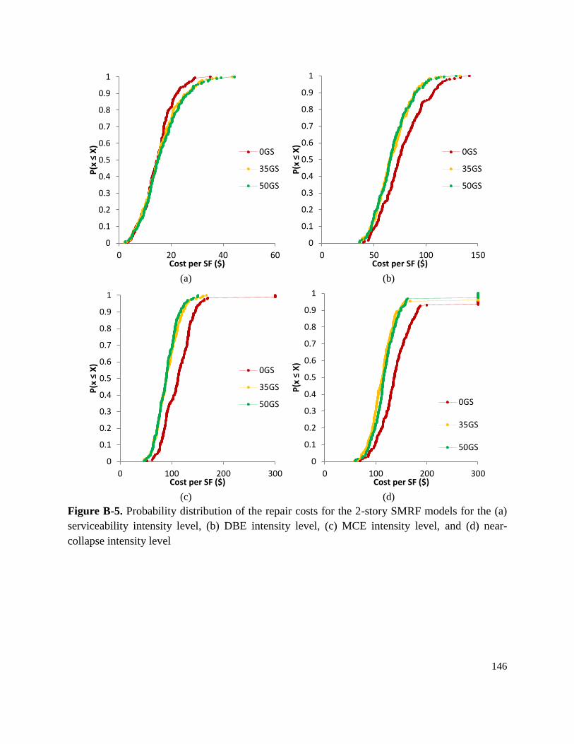
146

(a) (b)

(c) (d)

Figure B-5. Probability distribution of the repair costs for the 2-story SMRF models for the (a)



0

0.1

0.2

0.3

0.4

0.5

0.6

0.7

0.8

0.9

1

0 20 40 60

P(x

≤ X

)

Cost per SF ($)

0GS

35GS

50GS

0

0.1

0.2

0.3

0.4

0.5

0.6

0.7

0.8

0.9

1

0 50 100 150

P(x

≤ X

)

Cost per SF ($)

0GS

35GS

50GS

0

0.1

0.2

0.3

0.4

0.5

0.6

0.7

0.8

0.9

1

0 100 200 300

P(x

≤ X

)

Cost per SF ($)

0GS

35GS

50GS

0

0.1

0.2

0.3

0.4

0.5

0.6

0.7

0.8

0.9

1

0 100 200 300

P(x

≤ X

)

Cost per SF ($)

0GS

35GS

50GS

147

Table B-13. Average series repair time (in days) for the 2-story SMRF models with varying

levels of gravity connection strength

0GS 35GS 50GS

Serviceability 59 60 62

DBE 319 298 297

MCE 355 345 346

Near-collapse level 357 356 356

Table B-14. Total probability of receiving an unsafe placard for the 2-story SMRF models with

varying levels of gravity connection strength

0GS 35GS 50GS

Serviceability 0.04 0.05 0.03

DBE 0.98 0.92 0.90

MCE 0.99 0.98 0.98

Near-collapse level 1.0 1.0 1.0

Table B-15. Average number of casualties for the 2-story SMRF models with varying levels of

gravity connection strength

0GS 35GS 50GS


DBE 10 10 10

MCE 10 10 10


B.3.2. Four-Story Models

Figure B-6 shows the cost distributions for the 4-story models. Like the 2-story model, the

largest improvement can be seen at the higher intensity levels. The average cost was decreased

by nearly 32 percent under the near-collapse level intensity, by 29 percent under the MCE level,

and by 17 percent under the DBE level. Under the serviceability levels, the average cost actually

increased up to 7 percent when the partially restrained connections are modeled. The results

between the two levels of gravity connection strengths are similar, but the higher strength does

cause a larger decrease in cost for this structure. There was negligible difference between the

system with 35 percent strength and 50 percent strength.


and average number of casualties, respectively. The changes in repair time and probability of

receiving an unsafe placard are negligible. The average number of casualties is reduced under the

larger intensities. This reduction is up to 11 percent under the MCE and up to 23 percent under

the near-collapse level intensity. The median number of collapses is always zero.

148

(a) (b)

(c) (d)




0

0.1

0.2

0.3

0.4

0.5

0.6

0.7

0.8

0.9

1

0 10 20 30 40

P(x

≤ X

)

Cost per SF ($)

0GS

35GS

50GS

0

0.1

0.2

0.3

0.4

0.5

0.6

0.7

0.8

0.9

1

0 100 200 300

P(x

≤ X

)

Cost per SF ($)

0GS

35GS

50GS

0

0.1

0.2

0.3

0.4

0.5

0.6

0.7

0.8

0.9

1

0 100 200 300

P(x

≤ X

)

Cost per SF ($)

0GS

35GS

50GS

0

0.1

0.2

0.3

0.4

0.5

0.6

0.7

0.8

0.9

1

0 100 200 300

P(x

≤ X

)

Cost per SF ($)

0GS

35GS

50GS

149

Table B-16. Average series repair time (in days) for the 4-story SMRF models with varying


0GS 35GS 50GS


DBE 391 390 391

MCE 392 392 392




0GS 35GS 50GS


DBE 0.98 0.97 0.97

MCE 1.0 0.99 0.99




0GS 35GS 50GS


DBE 17 17 17

MCE 21 19 19


B.3.3. Eight-Story Models

Figure B-7 shows the cost distributions for the 8-story models. Like the previous models, the

largest improvement can be seen at the higher intensity levels, but the average costs decrease at

all intensity levels. The average cost was decreased by nearly 11 percent under the near-collapse

level intensity, by nearly 10 percent under the MCE level, by 10 percent under the DBE level,

and by more than 3 percent under the serviceability level. These reductions at the higher

intensities are less than those for the shorter structures.


and average number of casualties, respectively. The changes in repair time, probability of

receiving an unsafe placard, and number of casualties are negligible. The median number of

collapses is zero, except under the DBE level intensity. In this case, the median number of

casualties is 7 deaths.

150

(a) (b)

(c) (d)




0

0.1

0.2

0.3

0.4

0.5

0.6

0.7

0.8

0.9

1

0 10 20 30

P(x

≤ X

)

Cost per SF ($)

0GS

35GS

50GS

0

0.1

0.2

0.3

0.4

0.5

0.6

0.7

0.8

0.9

1

0 100 200 300

P(x

≤ X

)

Cost per SF ($)

0GS

35GS

50GS

0

0.1

0.2

0.3

0.4

0.5

0.6

0.7

0.8

0.9

1

0 100 200 300

P(x

≤ X

)

Cost per SF ($)

0GS

35GS

50GS

0

0.1

0.2

0.3

0.4

0.5

0.6

0.7

0.8

0.9

1

0 100 200 300

P(x

≤ X

)

Cost per SF ($)

0GS

35GS

50GS

151

Table B-19. Average parallel repair time (in days) for the 8-story SMRF models with varying


0GS 35GS 50GS


DBE 462 462 462

MCE 462 462 462




0GS 35GS 50GS


DBE 0.94 0.94 0.93

MCE 0.99 0.99 0.98




0GS 35GS 50GS


DBE 37 38 38

MCE 51 51 48


152

Appendix C: Ground Motions Used in “Response-History Analysis for the

Design of New Buildings: A Study of Assumptions” and “Accidental Torsion

in Nonlinear Response History Analysis.”

Numerous ground motion sets are used in the analyses for the research presented in the

manuscripts “Response-History Analysis for the Design of New Buildings: A Study of

Assumptions” and “Accidental Torsion in Nonlinear Response History Analysis.” While the

manuscripts provide the spectra of the ground motions sets, no further data is included, due to

space limitations. Primarily, tables are provided to summarize the ground motions used within

each record set. Table C-1 summarizes the ground motions used for the analysis of the MF2

Model, Table C-2 summarizes the ground motions used for the analysis of the MF8 Model,

Table C-3 summarizes the ground motions used for the SCAL and MTCH suites of the 3D

Model, Table C-4 summarizes the ground motions used for the 05CS suite of the 3D Model, and

Table C-5 summarizes the ground motions used for the 20CS suite of the 3D Model.

Additionally, acceleration time histories are provided for the spectrum matched ground motion

sets. The other time histories are provided in the NGA files previously tabulated; however, these

spectrum-matched time histories are developed using RSPMatch specifically for this work.

Figure C-1, C-2 and C-3 show the acceleration time histories for the spectrum matched ground

motions developed for the MF2 Model, the MF8 Model and the 3D Model, respectively.

Table C-1. Ground motions used for the analysis of the MF2 Model

NGA # Earthquake Name Moment

Magnitude

Distance

(km)

Vs30 - m/s

(Site Class) Source Type

Scale

Factor

169 Imperial Valley 06 6.5 22.0 275 (D) Strike Slip 2.7

313 Corinth, Greece 6.6 10.3 339 (D) Normal 3.2

829 Cape Mendocino 7.0 14.3 312 (D) Reverse 2.1

1236 Chi-Chi, Taiwan 7.6 37.5 273 (D) Reverse Oblique 4.0

161 Imperial Valley 06 6.5 10.4 209 (D) Strike Slip 3.2

573 Taiwan

SMART1(45) 7.3 76.4 275 (D) Reverse 4.0

959 Northridge-01 6.7 14.7 267 (D) Reverse 1.7

1048 Northridge-01 6.7 12.1 281 (D) Reverse 1.3

1208 Chi-Chi, Taiwan 7.6 24.1 442 (C) Reverse Oblique 3.6

1762 Hector Mine 7.1 43.1 271 (D) Strike Slip 4.0

3268 Chi-Chi, Taiwan 06 6.3 33.6 543 (C) Reverse Oblique 4.0

153

Table C-2. Ground motions used for the analysis of the MF8 Model


Magnitude

Distance

(km)

Vs30 -

m/s (Site

Class)

Source Type Scale

Factor

169 Imperial Valley-06 6.5 22.0 275 (D) Strike Slip 2.9

549 Chalfant Valley-02 6.2 17.2 271 (D) Strike Slip 4.0

573 Taiwan SMART1(45) 7.3 76.4 275 (D) Reverse 4.0

577 Taiwan SMART1(45) 7.3 78.2 275 (D) Reverse 4.0

728 Superstition Hills-02 6.5 13.0 194 (D) Strike Slip 3.8


1484 Chi-Chi, Taiwan 7.6 26.3 273 (D) Reverse Oblique 3.4

161 Imperial Valley-06 6.5 10.4 209 (D) Strike Slip 3.5

776 Loma Prieta 6.9 27.9 371 (D) Reverse Oblique 3.8


1762 Hector Mine 7.1 43.1 271 (D) Strike Slip 4.0

Table C-3. Ground motions used for the analysis of the 3D Model – SCAL and MTCH suites


Magnitude

Distance

(km)

Vs30 -

m/s Source Type

Scale

Factor

126 Gazli, USSR 6.80 5.5 660 Unknown 1.2

160 Imperial Valley-06 6.53 2.7 223 Strike-Slip 1.2



367 Coalinga-01 6.36 8.4 257 Reverse 2.2

496 Nahanni, Canada 6.76 4.9 660 Reverse 2.9

1004 Northridge-01 6.69 8.4 380 Reverse 0.9

1197 Chi-Chi, Taiwan 7.62 3.1 543 Reverse-Oblique 0.9



1605 Duzce, Turkey 7.14 6.6 276 Strike-Slip 1.2

154

Table C-4. Ground motions used for the analysis of the 3D Model – 05CS suite


Magnitude

Distance

(km)

Vs30 -

m/s Source Type

Scale

Factor




723 Superstition Hills-02 6.54 1.0 349 Strike-Slip 1.7

802 Loma Prieta 6.93 8.5 371 Reverse-Oblique 2.2



1063 Northridge-01 6.69 6.5 282 Reverse 1




Table C-5. Ground motions used for the analysis of the 3D Model – 20CS suite


Magnitude

Distance

(km)

Vs30 -

m/s Source Type

Scale

Factor





802 Loma Prieta 6.93 8.5 371 Reverse-Oblique 1.8

821 Erzican, Turkey 6.69 4.4 275 Strike-Slip 1.1

879 Landers 7.28 2.2 685 Strike-Slip 1.5





155

Figure C-1. Acceleration time histories of spectrum matched ground motions used to analyze the

MF2 Model, defined by NGA record used as the seed ground motion

-1

-0.5

0

0.5

1

0 50 100

Acc

eler

atio

n (

g)

Time (seconds)

SMGM - NGA 169

-1

-0.5

0

0.5

1

0 10 20 30 40

Acc

eler

atio

n (

g)

Time (seconds)

SMGM - NGA 313

-1

-0.5

0

0.5

1

0 10 20 30 40

Acc

eler

atio

n (

g)

Time (seconds)

SMGM - NGA 829

-1

-0.5

0

0.5

1

0 50 100

Acc

eler

atio

n (

g)

Time (seconds)

SMGM - NGA 1236

-1

-0.5

0

0.5

1

0 10 20 30 40

Acc

eler

atio

n (

g)

Time (seconds)

SMGM - NGA 161

-0.5

0

0.5

1

0 20 40Acc

eler

atio

n (

g)

Time (seconds)

SMGM - NGA 573

-1

-0.5

0

0.5

1

0 10 20 30

Acc

eler

atio

n (

g)

Time (seconds)

SMGM - NGA 959

-1

-0.5

0

0.5

1

0 10 20 30

Acc

eler

atio

n (

g)

Time (seconds)

SMGM - NGA 1048

-1

-0.5

0

0.5

1

0 50 100

Acc

eler

atio

n (

g)

Time (seconds)

SMGM - NGA 1208

-1

-0.5

0

0.5

1

0 20 40 60

Acc

eler

atio

n (

g)

Time (seconds)

SMGM - NGA 1762

-1

-0.5

0

0.5

1

0 20 40 60

Acc

eler

atio

n (

g)

Time (seconds)

SMGM - NGA 3268

156

Figure C-2. Acceleration time histories of spectrum matched ground motions used to analyze the

MF8 Model, defined by NGA record used as the seed ground motion

-1

-0.5

0

0.5

1

0 50 100

Acc

eler

atio

n (

g)

Time (seconds)

SMGM - NGA 169

-2

-1

0

1

0 10 20 30 40

Acc

eler

atio

n (

g)

Time (seconds)

SMGM - NGA 549

-0.5

0

0.5

1

0 20 40

Acc

eler

atio

n (

g)

Time (seconds)

SMGM - NGA 573

-1

0

1

0 20 40

Acc

eler

atio

n (

g)

Time (seconds)

SMGM - NGA 577

-1

-0.5

0

0.5

1

0 10 20 30 40

Acc

eler

atio

n (

g)

Time (seconds)

SMGM - NGA 728

-1

-0.5

0

0.5

0 20 40 60 80 100

Acc

eler

atio

n (

g)

Time (seconds)

SMGM - NGA 1198

-2

-1

0

1

0 20 40

Acc

eler

atio

n (

g)

Time (seconds)

SMGM - NGA 1484

-1

0

1

0 10 20 30 40

Acc

eler

atio

n (

g)

Time (seconds)

SMGM - NGA 161

-1

-0.5

0

0.5

1

0 20 40 60

Acc

eler

atio

n (

g)

Time (seconds)

SMGM - NGA 776

-1

-0.5

0

0.5

1

0 50

Acc

eler

atio

n (

g)

Time (seconds)

SMGM - NGA 1208

-1

-0.5

0

0.5

1

0 20 40 60

Acc

eler

atio

n (

g)

Time (seconds)

SMGM - NGA 1762

157

Figure C-3. Acceleration time histories of both components of spectrum matched ground

motions used to analyze the 3D Model, defined by NGA record used as the seed ground motion

-2

-1

0

1

0 10 20 30 40

Acc

eler

atio

n (

g)

Time (seconds)

SMGM - NGA 126

-2

-1

0

1

0 10 20 30 40

Acc

eler

atio

n (

g)

Time (seconds)

SMGM - NGA 160

-1

0

1

0 10 20 30 40

Acc

eler

atio

n (

g)

Time (seconds)

SMGM - NGA 165

-1

0

1

0 10 20

Acc

eler

atio

n (

g)

Time (seconds)

SMGM - NGA 189

-1

0

1

2

0 10 20 30 40Acc

eler

atio

n (

g)

Time (seconds)

SMGM - NGA 367

-1

0

1

0 10 20 30A

ccel

erat

ion

(g)

Time (seconds)

SMGM - NGA 496

-2

-1

0

1

2

0 10 20 30

Acc

eler

atio

n (

g)

Time (seconds)

SMGM - NGA 1004

-1

0

1

0 5 10 15 20

Acc

eler

atio

n (

g)

Time (seconds)

SMGM - NGA 1197

-1

0

1

2

0 20 40Acc

eler

atio

n (

g)

Time (seconds)

SMGM - NGA 1605

158

Appendix D: Fair Use Analysis Results

The next four pages contain Virginia Tech ETD Fair Use Analysis Results for Figures 2-8, A1,

A2 and A4.

Draft 09/01/2009

(Questions? Concerns? Contact Gail McMillan, Director of the Digital Library and Archives at Virginia Tech's University

Libraries: [email protected])

(Please ensure that Javascript is enabled on your browser before using this tool.)

Virginia Tech ETD Fair Use Analysis Results

This is not a replacement for professional legal advice but an effort to assist you in making a

sound decision.

Name: Jordan Jarrett

Description of item under review for fair use: Figure 2-8. Process of a Monte Carlo simulation Source: FEMA (2012).

Seismic Performance Assessment of Buildings, FEMA P-58, Applied Technology Council, Washington, D.C..

Report generated on: 12-12-2013 at : 20:51:57

Based on the information you provided:

Factor 1

Your consideration of the purpose and character of your use of the copyright work

weighs: in favor of fair use

Factor 2

Your consideration of the nature of the copyrighted work you used weighs: in favor

of fair use

Factor 3

Your consideration of the amount and substantiality of your use of the copyrighted

work weighs: in favor of fair use

Factor 4

Your consideration of the effect or potential effect on the market after your use of the

copyrighted work weighs: in favor of fair use

Based on the information you provided, your use of the copyrighted work weighs: in

favor of fair use

VT Fair Use Analysis Results http://etd.vt.edu/fairuse/analyzer/results.php

1 of 2 12/12/2013 8:52 PM

Draft 09/01/2009






sound decision.


Description of item under review for fair use: Figure A-1. Plan view of Performance Group 10 layout and an example

configuration of the lightning bolt bracing. Source: NIST (2010). Evaluation of the FEMA P-695 Methodology for

Quantification of Building Seismic Performance Factors, NIST GCR 10-917-8, NEHRP Consultants Joint Venture,

Redwood City, CA



Factor 1



Factor 2


of fair use

Factor 3



Factor 4




favor of fair use


1 of 2 12/12/2013 8:44 PM

Draft 09/01/2009






sound decision.


Description of item under review for fair use: Figure A-2. Typical plan view of the Collapse Prevention Systems

Source:Judd, J. and Charney, F. (2013). Seismic Collapse Prevention System. Unpublished Manuscript.



Factor 1



Factor 2

Your consideration of the nature of the copyrighted work you used weighs: against

fair use

Factor 3



Factor 4




favor of fair use


1 of 2 12/12/2013 8:46 PM

Draft 09/01/2009






sound decision.


Description of item under review for fair use: Figure A-4. Typical plan view of the SMRF systems Source: NIST (2010).

Evaluation of the FEMA P-695 Methodology for Quantification of Building Seismic Performance Factors, NIST GCR

10-917-8, NEHRP Consultants Joint Venture, Redwood City, CA.



Factor 1



Factor 2


of fair use

Factor 3



Factor 4




favor of fair use


1 of 2 12/12/2013 8:49 PM

performance assessment of seismic resistant steel structures · performance assessment of seismic...

Documents