performance assessment of porous asphalt for stormwater ......performance assessment of porous...
TRANSCRIPT

PERFORMANCE ASSESSMENT OF POROUS ASPHALT
FOR STORMWATER TREATMENT
BY
JOSHUA F. BRIGGS
B.S., University of Notre Dame, 1996
B.A., University of Notre Dame, 1996
THESIS
Submitted to the University of New Hampshire
in Partial Fulfillment of
the Requirements for the Degree of
Master of Science
in
Civil Engineering
December, 2006

This thesis has been examined and approved.
_______________________________________ Thesis Director, Dr. Thomas P. Ballestero Associate Professor of Civil Engineering
_______________________________________ Dr. Robert M. Roseen
Director, UNH Stormwater Center
_______________________________________ Dr. Jo Sias Daniel
Assistant Professor of Civil Engineering
_______________________
Date

ACKNOWLEDGEMENTS
First and foremost, I want to acknowledge my wonderful immediate family
– Dad, Mom, Susan, Megan, and Sarah. And my almost immediate family -
Benny and Tam. So many other good friends - Phu, Gregg B., Kim, Mirren, Yu-
Han, Amy, and the rest of the Sachems. Here in Durham, thanks to my many
good friends - Gabo, Pedro, Andrea, Jason, and Carolina. Thanks to Tom
(Lambert) for the bad jokes, and to his unfortunate roommates Linder and Birdie.
Sorry to my fellow cubicle mates for the obscenities…
I’d like to thank the UNH Stormwater Center, especially my advisor Tom
Ballestero, Rob Roseen, and Jamie Houle. They have been a constant source of
support, information, and good humor. And thanks to the rest of the dedicated
crew at the site – Pedro, Robert, Tim, Darlene, and Greg. Many others have
assisted me with my research along the way. Jo Daniel was invaluable in
bringing her knowledge of asphalt to this project. Michele Adams generously
reviewed our designs and provided the specifications used by her consulting firm,
Cahill Associates. Many others at UNH have helped me with small and not so
small things during the course of my stay here - Maddy, Kelly, Colleen, and Tom
K. And finally, thank you to Cooperative Institute for Coastal and Estuarine
Environmental Technology (CICEET) and National Oceanographic and
Atmospheric Agency (NOAA), who provide funding for the UNH Stormwater
Center.
iii

TABLE OF CONTENTS
ACKNOWLEDGEMENTS..................................................................................... iii LIST OF TABLES .................................................................................................vi LIST OF FIGURES ..............................................................................................vii LIST OF ABBREVIATIONS .................................................................................. x ABSTRACT .........................................................................................................xii
CHAPTER 1. BACKGROUND ............................................................................ 1 1.1 Introduction ....................................................................................... 1 1.2 Research Objective ........................................................................... 3 1.3 Description of Research .................................................................... 3 1.4 Study Area ........................................................................................ 6
CHAPTER 2. LITERATURE REVIEW ................................................................ 9 2.1 Design, Construction, and Cost......................................................... 9 2.2 Structural Durability, Life Cycle, and Cost ....................................... 21 2.3 Surface Infiltration Capacity, Clogging, and Maintenance............... 23 2.4 Winter Maintenance ........................................................................ 32 2.5 Hydraulic Performance.................................................................... 34 2.6 Water Quality Treatment & Retention of Pollutants......................... 40
CHAPTER 3. DESIGN, CONSTRUCTION, QA/QC, AND COST ..................... 48 3.1 Parking Lot Design, Construction, and QA/QC ............................... 48 3.2 Mix Design and In-Place Properties ................................................ 52 3.3 Cost Breakdown and Estimate for Typical Lot................................. 56
CHAPTER 4. METHODS AND MATERIALS .................................................... 59 4.1 Climate and Groundwater Data....................................................... 60 4.2 Pavement Durability and In-Place Mix Properties ........................... 62 4.3 Surface Infiltration Capacity ............................................................ 62 4.4 Frost Depth ..................................................................................... 66 4.5 Water Balance Analysis .................................................................. 67 4.6 Hydraulic Efficiency Analysis........................................................... 67 4.7 Water Quality Data Monitoring, Sampling, and Analysis ................. 68 4.8 Chloride Mass Balance Analysis ..................................................... 70
CHAPTER 5. RESULTS AND DISCUSSION.................................................... 75 5.1 Climate and Groundwater Data....................................................... 75 5.2 Pavement Durability ........................................................................ 80 5.3 Surface Infiltration Capacity ............................................................ 81 5.4 Frost Depth ..................................................................................... 88 5.5 Water Balance................................................................................. 91 5.6 Chloride Mass Balance ................................................................... 96
iv

5.7 Hydraulic Efficiency....................................................................... 103 5.8 Real-Time Water Quality Performance.......................................... 108 5.9 Discrete Sample Water Quality Performance................................ 113
CHAPTER 6. SUMMARY, RECOMMENDATIONS, AND CONCLUSIONS.... 122 6.1 Summary....................................................................................... 122 6.2 Recommendations for Future Research........................................ 124 6.3 Conclusions................................................................................... 125
REFERENCES................................................................................................. 127 APPENDICES .................................................................................................. 135 APPENDIX A. OGFC LITERATURE REVIEW ................................................. 136 APPENDIX B. UNH SPECIFICATION PACKAGE ........................................... 145 APPENDIX C. MATERIALS, QA/QC, COST, PAVEMENT CONDITION.......... 161 APPENDIX D. GROUNDWATER ELEVATION, WELLS, & SURFACE IC....... 166 APPENDIX E. HYDROGRAPHS & HYDRAULIC PERFORMANCE ................ 169 APPENDIX F. MEETING MINUTES, UNH GROUNDS & ROADS, 10/12/06... 180 APPENDIX G. REAL TIME WATER QUALITY STORM EVENT PLOTS ......... 184 APPENDIX H. LIST OF DATA FILES ON ATTACHED CD-ROM..................... 200
v
LIST OF TABLES
Table 1. Initial surface infiltration capacity for PA and OGFC............................. 24 Table 2. Volumetric and strength properties of PA and DMA samples. .............. 54 Table 3. Cost breakdown of UNH PA lot, and cost estimate of typical PA lot. .... 57Table 4. Surface IC statistics grouped by location and by location/season. ....... 84Table 5. Water balance between rainfall and PA effluent. .................................. 91 Table 6. UNH Grounds & Roads salt application data........................................ 97 Table 7. Chloride mass based on lineal loading by tarp experiment................. 100 Table 8. Chloride mass balance from 7/1/05 to 6/30/06. .................................. 100 Table 9. Hydraulic performance summary of the 4/20/05 event. ...................... 104 Table 10. Hydraulic performance summary for 12 storm events. ..................... 105 Table 11. Real time water quality EMC values for 12 storm events.................. 108 Table 12. Paired Student t-test on real time water quality EMC values. ........... 109 Table 13. Discrete sample water quality EMC and RE values for 12 events. ... 114Table 14. Paired Student t-test and Wilcoxon Rank Sum Test on discrete sample
water quality parameters. ................................................................ 114 Table 15. Chloride EMC values from analyzed samples and real time SC....... 118Table D-16. Surface IC via SIT, with raw and corrected values........................ 166 Table D-17. Groundwater elevations collected with manual sounder. .............. 167 Table D-18. Construction data for groundwater monitoring wells. .................... 168 Table E-19. Hydraulic performance summary of the 5/07/05 event.................. 169 Table E-20. Hydraulic performance summary of the 5/21/05 event.................. 170 Table E-21. Hydraulic performance summary of the 8/12/05 event.................. 171 Table E-22. Hydraulic performance summary of the 9/15/05 event.................. 172 Table E-23. Hydraulic performance summary of the 10/08/05 event................ 173 Table E-24. Hydraulic performance summary of the 11/30/05 event................ 174 Table E-25. Hydraulic performance summary of the 12/16/05 event................ 175 Table E-26. Hydraulic performance summary of the 1/11/06 event.................. 176 Table E-27. Hydraulic performance summary of the 3/13/06 event.................. 177 Table E-28. Hydraulic performance summary of the 5/01/06 event.................. 178 Table E-29. Hydraulic performance summary of the 6/01/06 event.................. 179
vi

LIST OF FIGURES
Figure 1. Aerial view of the DMA lot (left) PA lot (right), 11/04.............................. 5 Figure 2. Aerial view of the UNH Stormwater Center principal field site (upper
right) and its watershed, with PA site (lower left), 11/04. ..................... 7 Figure 3. Typical PA section (Cahill et al. 2004). ................................................ 10 Figure 4. Typical OGFC section (Tan et al. 1997). ............................................. 11 Figure 5. Idealized stormwater hydraulic performance characteristics. .............. 35 Figure 6. Cross section of UNH PA pavement.................................................... 48 Figure 7. Plan view of the UNH DMA lot with tree filter (left) and PA lot (top), by
Woodburn & Co., 9/01/04. ................................................................. 50 Figure 8. Gradation of crushed gravel for choker and reservoir courses. ........... 51Figure 9. Gradation of aggregate for PA and DMA mix designs. ........................ 53 Figure 10. Monitoring network and surface infiltration capacity test locations. ... 59Figure 11. Equipment for measuring IC via SIT (left) and DRI (right). ................ 64 Figure 12. Mean daily air temperature and precipitation for Durham, NH........... 76Figure 13. Daily snowfall, daily snow pack, and mean daily air temperature for
Durham, NH from 12/1/04 to 3/31/05. ............................................... 76 Figure 14. Daily snowfall and mean daily air temp from 11/1/05 to 3/31/06. ...... 77Figure 15. Groundwater elevations for pre-construction wells. ........................... 77 Figure 16. Groundwater and bed elevations for deep wells................................ 78 Figure 17. Groundwater and bed elevations for shallow in-system wells. .......... 78Figure 18. Real time water quality for groundwater wells. .................................. 79 Figure 19. Discrete sample water quality for groundwater wells......................... 79 Figure 20. Pavement photographs, summer 2005. Plow scars (left), collapsed
pavement between well boxes (right). ............................................... 81 Figure 21. Surface IC time series (left) and box plot (right). ............................... 82 Figure 22. Residual sand and salt mix on PA lot, winter 2005. Clumped mix (top)
and close up of mix (bottom). ............................................................ 85 Figure 23. Other observed particulate sources; plow-abraded PA aggregate (top
left), bark mulch (top right), and speed bump material (bottom). ....... 87 Figure 24. Frost depth and air temperature for March, 2005. ............................. 89 Figure 25. Frost depth, with min. and max. air temp. for winter, 2006. ............... 90 Figure 26. Monthly water balance and ratio of precipitation to effluent............... 92 Figure 27. Cumulative water balance. ................................................................ 92 Figure 28. Groundwater elevations for Wells 5m and 5d, and differences in
elevation as indicator of infiltration or exfiltration. .............................. 94 Figure 29. SC time series for D-Box and PA effluent from 7/1/05 to 6/30/06 (top)
and for the winter with salt application events (bottom)..................... 99 Figure 30. Monthly chloride mass balance from 7/1/05 to 6/30/06. .................. 101 Figure 31. Cumulative chloride mass balance from 7/01/05 to 6/30/06. ........... 101 Figure 32. Hydrograph and hyetograph of the 4/20/05 event. .......................... 104
vii
Figure 33. Peak reduction coefficient (kp) regression plots............................... 107 Figure 34. Lag coefficient (kL) regression plots................................................. 107 Figure 35. Box plots of real time water quality EMC values for 12 events. ....... 109Figure 36. SC time series of D-Box and PA effluent for the 1/11/06 event. ...... 111Figure 37. Median RE values for discrete sample parameters. ........................ 113 Figure 38. Treatment effect plots of discrete sample EMC values.................... 115 Figure 39. Box plots of discrete sample EMC values. ...................................... 116 Figure 40. PA effluent probability plots of discrete sample EMC values........... 117Figure B-41. UNH PA specification package. ................................................... 160 Figure C-42. PG asphalt binder certification, Pike Industries, 7/08/04.............. 161 Figure C-43. Field notes from date of asphalt placement, Jo Daniel, 10/13/04.162Figure C-44. Mix design report, Pike Industries, 10/07/04................................ 162 Figure C-45. Gradation of bank run gravel used as the filter course. ............... 163 Figure C-46. Paving quote, alternates by binder type, Pike Industries, 7/14/04.
........................................................................................................ 164Figure C-47. Memo on PA pavement condition, Jo Daniel, 6/24/05. ................ 165 Figure D-48. Groundwater monitoring well profile sketch. Hatched areas are
either ground surface (top) or bottom of bed (lower). Elev. in ft MSL......................................................................................................... 168
Figure E-49. Hydrograph and hyetograph of the 5/07/05 event........................ 169 Figure E-50. Hydrograph and hyetograph of the 5/21/05 event........................ 170 Figure E-51. Hydrograph and hyetograph of the 8/12/05 event........................ 171 Figure E-52. Hydrograph and hyetograph of the 9/15/05 event........................ 172 Figure E-53. Hydrograph and hyetograph of the 10/08/05 event...................... 173 Figure E-54. Hydrograph and hyetograph of the 11/30/05 event...................... 174 Figure E-55. Hydrograph and hyetograph of the 12/16/05 event...................... 175 Figure E-56. Hydrograph and hyetograph of the 1/11/06 event........................ 176 Figure E-57. Hydrograph and hyetograph of the 3/13/06 event........................ 177 Figure E-58. Hydrograph and hyetograph of the 5/01/06 event........................ 178 Figure E-59. Hydrograph and hyetograph of the 6/01/06 event........................ 179 Figure F-60. Meeting minutes, UNH Grounds & Roads, 10/12/06.................... 183 Figure G-61. Box plots of real time water quality for 4/20/05............................ 184 Figure G-62. Box plots of real time water quality for 5/07/05............................ 184 Figure G-63. Box plots of real time water quality for 5/21/05............................ 184 Figure G-64. Box plots of real time water quality for 8/12/05............................ 185 Figure G-65. Box plots of real time water quality for 9/15/05............................ 185 Figure G-66. Box plots of real time water quality for 10/08/05. ......................... 185 Figure G-67. Box plots of real time water quality for 11/30/05. ......................... 186 Figure G-68. Box plots of real time water quality for 12/16/05. ......................... 186 Figure G-69. Box plots of real time water quality for 1/11/06............................ 186 Figure G-70. Box plots of real time water quality for 3/13/06............................ 187 Figure G-71. Box plots of real time water quality for 5/01/06............................ 187 Figure G-72. Box plots of real time water quality for 6/01/06............................ 187 Figure G-73. Time series plots of real time water quality for 4/20/05................ 188 Figure G-74. Time series plots of real time water quality for 5/07/05................ 189 Figure G-75. Time series plots of real time water quality for 5/21/05................ 190
viii

Figure G-76. Time series plots of real time water quality for 8/12/05................ 191 Figure G-77. Time series plots of real time water quality for 9/15/05................ 192 Figure G-78. Time series plots of real time water quality for 10/08/05.............. 193 Figure G-79. Time series plots of real time water quality for 11/30/05.............. 194 Figure G-80. Time series plots of real time water quality for 12/16/05.............. 195 Figure G-81. Time series plots of real time water quality for 1/11/05................ 196 Figure G-82. Time series plots of real time water quality for 3/13/05................ 197 Figure G-83. Time series plots of real time water quality for 5/01/05................ 198 Figure G-84. Time series plots of real time water quality for 6/01/05................ 199
ix

LIST OF ABBREVIATIONS
AASHTO American Association of State Highway and Transportation Officials
ASTM American Society for Testing and Materials BMP Best Management Practice BOD Biological Oxygen Demand Cd Cadmium CICEET Cooperative Center for Coastal and Estuarine Environmental
Technology Cl Chloride COD Chemical Oxygen Demand Cr Chromium CRREL Cold Regions Research and Engineering Laboratory
(U.S. Army Corps of Engineers) Cu Copper CWP Center for Watershed Protection D-Box Distribution Box DL Detection Limit DMA Dense Mix Asphalt DO Dissolved Oxygen DOT Department of Transportation DRI Double Ring Infiltrometer EMC Event Mean Concentration EPA Environmental Protection Agency GPM Gallons per Minute HDPE High Density Polyethylene HMA Hot Mix Asphalt ID Inner Diameter IC Infiltration Capacity LID Low Impact Development NAPA National Asphalt Pavement Association NCAT National Center for Asphalt Technology NCDC National Climatic Data Center NH New Hampshire NOAA National Oceanic and Atmospheric Agency NO3-N Nitrate as Nitrogen NPDES National Pollutant Discharge Elimination System OGFC Open Graded Friction Course PA Porous Asphalt PAH Polyaromatic Hydrocarbon Pb Lead
x

PEM Permeable European Mix PG Performance Grade PSU Pennsylvania State University PVC Polyvinyl Chloride QA/QC Quality Assurance/ Quality Control RE Removal Efficiency RLI Resource Laboratories, Inc. SC Specific Conductivity SIT Surface Inundation Test Total P-P Total Phosphorus as Phosphorus TPH-D Total Petroleum Hydrocarbons as Diesel TRB Transportation Research Board TSS Total Suspended Solids UNH University of New Hampshire UK United Kingdom UNHWS UNH Weather Station URI University of Rhode Island VAOT Vermont Agency of Transportation Zn Zinc
xi

ABSTRACT
PERFORMANCE ASSESSMENT OF POROUS ASPHALT FOR STORMWATER TREATMENT
by
Joshua Fowler Briggs
University of New Hampshire, December 2006
The objective of this study is to assess the stormwater management
capability of porous asphalt (PA) as a parking lot in Durham, New Hampshire.
The site was constructed in 2004 and consists of a 4-inch PA pavement course
overlying a porous media reservoir, including a fine-grained filter course. Cost
per PA parking space ($2,200) was comparable to that for dense mix asphalt
($2,000). Pavement durability has been adequate. The lot retained or infiltrated
25% of precipitation (18 months) and 0.03 lb/sf of chloride (1 year). There was
high initial surface infiltration capacity (IC) at two locations (1,000 – 1,300 in/hr),
and moderate IC at a third (330 in/hr). Two locations had a 50% decrease in IC.
Frost penetration occurred to 1 foot. Storm event hydraulic performance was
exceptional. Storm event water quality treatment for diesel, zinc, and TSS were
excellent; for chloride and nitrate it was negative, and for phosphorus, limited.
xii

CHAPTER 1
BACKGROUND
1.1 Introduction
Stormwater management has grown immensely in importance and scope
over the past few decades. Recent implementation of the National Pollutant
Discharge Elimination System (NPDES) Phase II rules under the Clean Water
Act requires the design and implementation of local stormwater management
plans. One of the requirements under these rules is the use of Best
Management Practices (BMP), measures to treat water quality and water
quantity of stormwater runoff from developed sites. Common BMPs include wet
and dry detention ponds and swales. Water quantity issues have been
somewhat successfully addressed by BMPs on a site scale with outlet control
devices. But watershed-scale water quantity impacts of multiple BMPs have not
been adequately addressed. And the BMPs often further degrade water quality
of the pollutant-laden stormwater runoff from impervious surfaces.
Investigations by Ballestero et al. (2000) found that the performance of
traditional storm water control systems (retention pond, detention pond, grassed
swale) in coastal New Hampshire (NH) had a high degree of failure for at least
one type of contaminant. Failure was defined as effluent concentrations
1

exceeding influent concentrations during the first flush. For a wide range of
contaminants there was no clear trend of positive performance.
In light of the poor performance record of BMPs, other types of devices
and technologies have grown in popularity. Recently, Low Impact Development
(LID) treatments have become more popular as driven by the need for more
water quality treatment. LID is an innovative stormwater management approach
that manages rainfall (preferably at the source) using distributed decentralized
infiltration mechanisms. Porous pavements are one class of LID treatment that
can address both stormwater quality and quantity issues. Porous pavements
consist of a permeable (porous, pervious) surface course underlain by a porous
media reservoir. In this case, the filter course of the porous media reservoir was
selected to provide water quality treatment. Common materials used for
pavement surface are plastic-reinforced turf grids, concrete pavers, porous
concrete, and PA (Ferguson 2005). The net effect of filtration and retention of
pollutants in the surface layer, and quantity treatment in the porous media
reservoir usually leads to an improvement in stormwater management.
In light of the mixed record of stormwater BMPs, the University of New
Hampshire (UNH) Stormwater Center set out to test traditional BMPs,
manufactured devices, and LID designs. There are 12 technologies tested in
parallel at the main research site (Roseen et al. 2006), and a secondary research
facility was constructed with two parking lots: one with PA and another
conventional parking lot as a control standard. Construction of the PA facility
used the most current mix designs available at the time (Kandhal 2002, Jackson
2

2003, VAOT 2004, Adams 2004). The facility was completed in October, 2004,
and the fully monitored by April, 2005. This thesis summarizes the stormwater
management performance of the PA parking lot from construction through
October, 2006.
1.2 Research Objective
The purpose of this study was to document design, construction, and cost,
and to assess performance of a PA parking lot at UNH as both a stormwater
management technology and commuter parking lot. Short term performance of
the facility was evaluated by measurement of surface infiltration capacity (IC),
frost penetration, water balance, and chloride mass balance. Storm event
performance was assessed by hydraulic efficiency and water quality treatment.
Water quality analyses included both real time and discrete sample parameters.
Short term performance as a commuter parking lot was assessed for pavement
mix design/properties and pavement durability.
1.3 Description of Research
Substantial efforts were undertaken by members of the UNH Stormwater
Center to make the PA facility a reality before data collection and analysis began
for this thesis. In early 2004, a literature review was conducted to obtain site
assessment criteria, design specifications, construction and maintenance
considerations, and monitoring designs for PA pavement. After gathering this
information from various sources, assessment was undertaken at two sites on
3

the UNH campus. Site assessment tasks included a topographic and wetland
survey, a wetland survey, groundwater monitoring, and test pits for identifying
soils and measuring soil infiltration capacities. After several meetings with UNH
officials, in late spring 2004, the West Edge Lot site was selected.
Specifications and drawings were completed by early summer 2004. After
several review iterations, the bid package was prepared and released. PA mix
specifications were based on information from the Vermont Agency of
Transportation (VAOT), National Asphalt Pavement Association (NAPA)
publication ISI-131 (Kandhal 2002), and conversations with Michele Adams from
Cahill Associates. Aggregate gradation, asphalt content, and draindown
specifications were based on NAPA recommendations. The plant and production
specifications were based largely on VAOT Section 400. The PA filter course
material was selected for structural (load bearing) and water quality (filtration)
requirements. A locally available bank run gravel met both needs.
By late summer, a bidder had been selected, and construction planning
commenced. Construction occurred over an approximate three week period in
late September and early October, 2004. Construction proceeded smoothly,
largely due to contractor familiarity with the site and design, low precipitation, and
low groundwater levels. By late October 2004, the lot was open for commuter
parking (Figure 1).
The PA monitoring plan that had been developed during the previous
months was then implemented. Site visits began to occur frequently and
photographs were taken regularly to document pavement condition and
4

DMA
PA
Figure 1. Aerial view of the DMA lot (left) PA lot (right), 11/04.
monitoring status, particularly during storm events. Surface IC testing began in
November. Several groundwater wells were installed in December 2004,
replacing the three groundwater wells destroyed during construction. These
wells were developed over the following weeks, and a groundwater sampling
routine began. In situ level and temperature loggers were installed and began
collection data by early February 2005. Manual groundwater level soundings
and transducer data uploads began to occur on an approximately monthly basis.
A frost gauge was constructed and deployed in Well 5s. Well 5s was ideal for a
frost gauge, since it was situated in the center of the PA lot and the screened
level consistently above the groundwater table. In late February and March
2005, the frost gauge was removed, and temperature loggers were deployed at
different depths in the Well 5s to measure frost penetration in and below the
5

pavement. Frost depth readings were collected on an approximately weekly
basis.
In early 2005, monitoring equipment for flow measurement and water
quality monitoring was installed in Well 1. Well 1 is an angled well on the edge of
the PA facility. After two months of real time data collection, it became evident
that melt water infiltration was biasing groundwater levels and water quality
readings that were meant to be representative of the PA system as a whole. The
monitoring location was then moved to the PA underdrain pipe (effluent). Real
time monitoring began in earnest on April 1, 2005. Data collection for this device
and in other research areas noted above continued until the present.
1.4 Study Area
The study was performed at the UNH Stormwater Center’s PA site and
principal field site (main site). Both are located on the perimeter of a 9-acre
commuter parking lot (West Edge Lot) at UNH in Durham, NH (Figure 2). The
West Edge Lot is standard dense mix asphalt (DMA), installed in 1996, and is
used near capacity throughout the academic year, excepting student vacation
periods during holidays and summer. The watershed area is large enough to
generate substantial runoff, which is gravity fed through conventional stormwater
catch basins and sewers. Sewers from the parking lot catch basins converge
into a larger 36-inch reinforced concrete pipe that connects to the 10-foot square
concrete distribution box (D-Box). This pipe is monitored several feet upstream
of the entrance to the D-Box for level/flow, real time water quality, and is sampled
6

during selected storm events. For the purposes of assessing water quality
performance of the PA stormwater treatment site, this is the ‘influent’.
The parking lot is partially curbed and entirely impervious. The watershed
area is mostly impervious, although a small percentage (<3%) does receive
runoff from offsite wooded areas. Vehicle activity is a combination of passenger
vehicles and routine bus traffic. The runoff time of concentration for the lot is 22
minutes, with slopes ranging from 1.5-2.5%. The area is subject to frequent
plowing, salting, and sanding during the winter months.
Field Facility at theField Facility at theUNH WEST EDGE LOTUNH WEST EDGE LOT
Tc ~ 22 minutesTc ~ 22 minutes
POROUS ASPHALT
CSTEV RESEARCH FACILITY
TREEFILTER
Watershed Boundary
WATERSHED BOUNDARY
DMA LOT W/ TREE FILTER
POROUS ASPHALT
LOT
CSTEV RESEARCH FACILITY
Figure 2. Aerial view of the UNH Stormwater Center principal field site (upper right) and its watershed, with PA site (lower left), 11/04.
7

The PA site is attached to the opposite (east) side of the West Edge Lot,
but is hydrologically isolated (Figure 1). The watershed area is approximately
5,600 ft2 (0.12 ac), almost all of which is highly permeable PA pavement. The PA
lot has 18 parking spaces. The PA facility receives negligible stormwater runoff
from outside of the curbed area surrounding the PA pavement. During snowmelt
events in winter, however, considerable melt water from snow banks can enter
the facility through the highly permeable rock-lined shoulder surrounding the PA
facility.
Immediately adjacent, identically sized, and hydrologically separated from
the PA facility is the DMA lot with tree filter. This lot is equally sized and situated
to act as a hydraulic control with which to compare the PA lot. The tree filter is
another of the several innovative and conventional stormwater treatment
technologies studied by the UNH Stormwater Center. The DMA lot has 16
parking spaces, and is separated from the PA lot by a speed bump. The DMA lot
was the control for comparisons of cost, pavement mix properties, and pavement
durability with PA.
Average annual precipitation is 48 inches uniformly distributed throughout
the year, with average monthly precipitation of 4.0 inches +/- 0.5. The mean
annual temperature is 48°F, with the average low in January at 16°F, and the
average high in July at 83°F (Roseen et al. 2006). Aerially-weighted precipitation
was used for water balance and hydraulic efficiency analysis.
8

CHAPTER 2
LITERATURE REVIEW
This chapter is a review of the literature relating to design, construction,
cost, maintenance, and performance aspects of PA pavement and other
permeable pavements. Open graded friction course (OGFC) is introduced and
discussed in this chapter where it shares common attributes with PA. Detailed
information unique to OGFC is provided in Appendix A.
2.1 Design, Construction, and Cost
2.1.1 Background
Porous asphalt herein refers to the permeable asphalt pavement layer and
the underlying porous media reservoir typically used at parking lots for
stormwater management objectives (Figure 3). PA system components include
a top filter course (setting bed), filter course, storage course, geotextile filter
fabric, existing soil or subgrade material, and optional bottom filter course
(Jackson 2003). OGFC is an open-graded hot mix asphalt (HMA) mixture with
interconnecting voids that is placed over an impermeable base (Figure 4).
OGFC is used on highways to facilitate rapid drainage of runoff to the shoulder
during rainfall. OGFC is not equivalent to PA as discussed in this thesis. While
the asphalt mixes for the PA and OGFC are often identical, the application and
9

whole system design are distinctly different. The principal difference between the
PA and OGFC is that the PA (by design) allows surface water to drain through
the porous media reservoir. OGFC permits near surface drainage only with no
surface water infiltration to the road base.
Cahill Associates is the most experienced designer of PA parking lots.
They have published numerous guidelines, articles, and presentations on this
subject, many of which are freely available from their website (www.thcahill.com).
Engineering of PA involves suitability assessment, system design, asphalt
mix design, mix production, hauling, and construction. Each of these subjects is
discussed in the following subsections.
Figure 3. Typical PA section (Cahill et al. 2004).
10

Figure 4. Typical OGFC section (Tan et al. 1997).
2.1.2 Suitability
Appropriate consideration of site conditions is critical to the success of a
PA project. Jackson (2003) stated that site considerations for PA include a
number of factors related to soil condition and geology: soil type, soil infiltration
capacity, depth to bedrock, and depth to water table. Other important
considerations include slope and frost susceptibility. Others are listed below as
encountered in the literature review.
Subgrade soil type & soil infiltration capacity: Jackson (2003) advocated
use of upland soils, which are typically well to moderately well drained. Field-
verified IC of soils below the bottom of the porous media reservoir in the literature
ranged from 0.1 in/hr to 3 in/hr (Environmental Protection Agency (EPA) 1999,
Center for Watershed Protection (CWP) 2004, Jackson 2003). Lower soil IC
11
limits are set to ensure that infiltrate does not pool at the base of the porous
media reservoir. Upper soil IC limits are set to ensure that adequate water
quality treatment, such as filtration, occurs before water infiltrates.
Depth to bedrock and seasonal high water table: Minimum depth to
bedrock in the literature ranged from 2 feet (Jackson 2003) to 4 feet (EPA 1999).
Minimum depth to seasonal high groundwater in the literature ranged from 2 to 5
feet (EPA 1999, CWP 2004, Jackson 2003). Depths are relative to the base of
the porous media reservoir. Minimum depths to bedrock and high water table
are established in order to ensure that adequate water quality treatment occurs in
the subgrade soils. In the case where a fine-grained filter course (not gravel) is
used on a subbase, separation could be measured from the top of the filter bed.
This provides credit for filter courses that provide water quality treatment.
Local topography: EPA (1999) recommended that slopes on a PA site
should be flat or very gentle (less than 5%). However, Cahill Associates has
successfully installed PA lots in hilly terrain by using terraced porous media
reservoirs and DMA paving of steep access roads (Jackson 2003). The use of
flat bottom reservoirs maximizes the potential for infiltration into the subgrade
soils. Systems with sloped reservoir bottoms and course grained materials must
be designed with care to prevent excessive flow and possible soil piping at this
location.
Climate: Porous pavement is suitable for cold climates provided design
considerations are met. Caution should be used in siting porous pavements in
cold regions due to the issues with sand application (clogging) and chloride
12
contamination of groundwater (CWP 2004). Frost heave has been cited as an
issue, but extending pavement to below the frost depth reduces the risk (CWP
2004, Jackson 2003). Ensuring that the pavement is well drained either with
underdrains, or by addition of a coarse grained capillary barrier between the
reservoir base and native soils will reduce frost heave. These methods allow the
water to drain freely so as not to collect, freeze, and cause damage to overlying
pavement by expansion. Porous pavements might be restricted in arid regions
and those with high rates of wind-blown sediments, due to potential clogging
issues (EPA 1999, Jackson 2003). However, the only PA highway installed in
the US is located in Arizona, and was functioning (at least structurally) as of 2005
(Ferguson 2005).
Traffic and proposed land use: Porous pavement are appropriate
substitutes for conventional pavement on parking areas, light traffic areas, low
use roadways, and even shoulders of airport taxiways and runways provided
other site conditions are met (EPA 1999). CWP (2004) explained that
stormwater hotspots, areas where land use or activities generate highly
contaminated runoff, should be avoided due to the rapid infiltration of stormwater
inherent to porous pavements. Rapid infiltration of contaminated stormwater
runoff, such as a gasoline spill, would require costly removal. For cost and
constructability reasons, porous pavements could be used best for stormwater
retrofits on individual sites where the parking lot needs resurfacing anyway (CWP
2004). Jackson (2003) suggested that PA is ideally suited to recreational areas
such as basketball and tennis courts or infrequently used sport complex parking
13
lots. Traffic volume increases wear on PA, which typically has less strength than
DMA.
Water supply wells: Consistent with the guidelines for infiltration systems,
The use of porous pavements should be restricted (100 feet setback) in
groundwater drinking supply areas due to the poor treatment performance for
nitrates and chlorides (EPA 1999, CWP 2004).
Site size: Drainage area should be less than 15 acres (EPA 1999). No
justification was provided for this recommendation, and other literature sources
did not comment on drainage area.
Cold water streams: Porous pavements can be used to reduce
temperatures of runoff that can negatively impact sensitive receiving waters
(CWP 2004). During the summer, elevated runoff temperature can be
substantially lowered by infiltration through the cooler porous media reservoir due
to the large mass for thermal transfer.
Governmental regulations: Jackson (2003) stated that in the absence of
local or state regulations, typical designs should treat/detain the 6-month/24-hour
storm event for the drainage area. More conservative criteria would treat/detain
the 25-year/24-hour storm event. NPDES requirements may also dictate where,
when, and how a PA parking lot may be employed. Recently, the Pennsylvania
Stormwater Best Management Practices Manual (2006) recommended the
following runoff control guidelines for post-development conditions:
1. Total runoff volume shall not increase for all storms equal to or
less than the 2-year/24-hour event.
14
2. Peak rate of runoff shall not increase for the 1-year through 100-
year storms
3. Water quality reduction shall be at least 85% for TSS, 85% for
total phosphorus as phosphorus (Total P-P), and 50% for nitrate
(NO3-N).
2.1.3 System Design
PA design components vary depending on specification source. Jackson
(2003) described the PA design components. The PA course should be open
graded asphalt concrete with void space of greater than 18% (typically ranging
up to 20%) and thickness ranging from 2 to 4 inches. Desirable mix properties
will be discussed in Section 2.1.4. The top filter course should be a minimum of
2 inches thick and contain 0.5 inch crushed stone aggregate. The “reservoir
course” is a base course of crushed stone. Depth of the reservoir course is
determined as the greatest depth as calculated for storage volume, structural
requirements, and frost depth. Minimum thickness is 8 to 9 inches. Aggregate
size is typically 1.5 to 3 inches, and American Association of State Highway and
Transportation Officials (AASHTO) No. 2 gradation is often specified. In place
void space after compaction is approximately 40%. Smaller aggregate (e.g.
AASHTO No. 5) sizes may be utilized, provided that requisite calculated
minimum depths are met.
The subsurface soils should drain the reservoir in 48 to 72 hours. The
engineer must select the appropriate reservoir depth, aggregate type and
15

porosity, and underdrain (if necessary) to meet this objective in light of
subsurface infiltration capacities. Adjacent impervious areas may also be routed
directly to the reservoir for stormwater management purposes. Reservoir sizing
would need to reflect the additional inflow of stormwater. A filter fabric
(geotextile) can be laid on top of the undisturbed subgrade soils to prevent fines
from migrating into the reservoir. The geotextile also provides structural support
for the reservoir course. The geotextile fabric may also impede downward
percolation of water into the subgrade. There is reportedly clogging occurring at
the geotextile layer at the University of Rhode Island (URI) PA lot in Kingston,
Rhode Island (Boving et al. 2004).
2.1.4 Mix Materials and Design
Mix design and materials are identical for PA and OGFC. Huber (2000)
provided a comprehensive survey of mix material and design in the US and in
Europe. He recommended that a new mix design method be formulated that
include air void content as a criterion, durability test such as the Cantabro test,
and compaction using the Superpave gyratory compactor. The four mix design
steps were as follows: (1) materials selection, (2) selection of design gradation,
(3) determination of optimum asphalt content, and (4) evaluation for moisture
susceptibility. There are extensive detailed requirements that are to be met
when undertaking mix design.
Jackson (2003) recommended that the high temperature binder grade be
increased by two grades to prevent scuffing (i.e. if a Performance Grade (PG)
16

PG 64-22 is specified for DMA in the region, a PG 76-22 should be used with
PA/OGFC). Scuffing is a type of pavement distress whereby the mix is
deformed, and is typically caused by turning of automobile tires, especially at low
speeds. The use of polymer modified asphalt, asphalt rubber, and fibers have
been effective in increasing the strength and decreasing binder draindown of
OGFC and PA. The common polymer modifier is styrene-butadiene-styrene
(SBS). Draindown of less than 0.3% is preferred. Asphalt content is typically 6
to 6.5% by total mix weight. Actual asphalt content should be based on a mix
design utilizing locally supplied aggregate and mix design guidelines for OGFC.
2.1.5 Mix Production, Hauling, and Placement
Mix production, hauling, and placement are identical for PA and OGFC.
This section addresses production of the mix, modifications to the asphalt plant
(as necessary), hauling, and placement at the project site. In general, few
specific plant modifications are required for open-graded mixes. Huber (2000)
reported that any plant capable of producing a high quality DMA mix can produce
a high quality PA/OGFC mix. Aggregates stockpiles are handled with the same
procedures as DMA.
The main modification to asphalt production plants are the detailed
aggregate gradation and mixing requirements for any additives used such as
fibers or polymers. Fibers are added either in pelletized or loose form, and both
can be added in either batch or drum plants. Fiber addition must be calibrated in
order to ensure consistency within the asphalt mix. During asphalt plant
17

production, fibers must be metered and evenly distributed throughout the binder.
The binder must sometimes be agitated in the asphalt storage tank to ensure
mixing. Mixing temperature must be kept high so that complete coating of
aggregate occurs, but not so high that binder draindown occurs. Oregon
Department of Transportation (DOT) limits mixing temperature to 320°F for
unmodified asphalt binder and to 347°F for modified asphalt. The asphalt
mixture should not be stored in surge bins or silos for extended periods due to
potential draindown issues.
Kandhal (2002) described the hauling procedure. If the mix is polymer
modified, a thick coat of asphalt release agent must be applied to truck beds.
This release agent must be completely removed after offloading the mix by
raising the truck bed and allowing it to drain. It is important to limit haul distance
(e.g. Oregon DOT limits haul distance from 35 to 50 miles) so that cooling of the
high air void mixture is not excessive and does not lead to cold lumps. Tarping is
also required to prevent crusting and cold spots in the mix. Great care should be
taken in coordinating a smooth progression from production, hauling, and
placement in order to prevent excessive cooling of the PA/OGFC.
Oregon DOT specified a minimum allowable placement temperature of
205°F for their OGFC mix (Moore et al. 2001). California’s DOT (CALTRANS
2006) dictated OGFC placement temperature for breakdown and finish rolling
based on air temperature and on whether the mix was modified or not. For an
OGFC polymer modified binder with air temperature at placement ranging from
45 to greater than 70°F, rolling should be completed before the temperature of
18

the OGFC drops below 250°F. For air temperatures at placement greater than
70°F, rolling of OGFC with unmodified binder should be completed before OGFC
falls below 195°F. The minimum allowable air temperature for placement of
OGFC with unmodified binder should be 55°F.
2.1.6 Construction
This section summarizes the process for constructing PA parking lots.
More information can be found at Cahill Associates’ website (www.thcahill.com)
and in NAPA’s guidance document (Jackson 2003). A brief summary of this
process and guidelines follow.
As contractors are generally unfamiliar with PA construction, thorough and
timely oversight is essential to the success of PA projects. Phasing of PA
construction is important, and its actual construction should typically fall towards
the end of any other site work. The porous media reservoir excavation can often
serve as a temporary sedimentation basin during construction (Jackson 2003).
Jackson (2003) provided additional guidelines as follows:
• The site (especially subgrade soils) should be protected from
excessive compaction due to heavy equipment by use of low earth
pressure equipment.
• The filter layer, consisting of a geotextile filter fabric with optional 2-
inch thick lower filter course of 0.5-inch aggregate, should be
placed on uncompacted subgrade soil. There is no consensus in
the literature on the use of geotextile at the interface with the
19
porous media reservoir and the native soils, and thus is not always
recommended.
• Clean, washed 1.5- to 3-inch size aggregate should be placed in
the reservoir in 6-inch lifts. Each lift should be compacted with
plate compactors or lightweight rollers. Minimum reservoir course
thickness is 8 to 9 inches.
• A 1- to 2-inch thick top filter course layer of 0.5-inch crushed
aggregate should be placed over the reservoir course, and then
compacted.
• A 2- to 4-inch thick single course of PA mix should be placed
following guidelines in the specification for open graded mixes.
Failures at this step can lead to premature hardening of the asphalt
and early mix failure due to raveling or loss of IC.
• Asphalt should be rolled in two to three passes with a 10-ton steel
wheel roller. More frequent rolling could lead to overcompaction,
decreased air void content, decreased IC, and increased
susceptibility to clogging.
• After rolling, traffic should be prohibited for 24 hours.
• For the life of the project, the PA pavement should be protected
from construction debris and sediment-laden water from off-site.
• Once construction is completed and vegetation is established,
temporary erosion and sediment control facilities should be
removed.
20

• Signage is an important part of the construction process. At a
minimum, signs should inform maintenance personnel of the
special requirements for PA. These include a prohibition on
sealing, as well as keeping sand and debris off of pavement (see
maintenance section). The signs can also be used to educate the
public.
2.2 Structural Durability, Life Cycle, and Cost
A review of the extensive literature on structural durability of PA over the
past 30 years finds many examples of successes and failures. In general,
successful examples of durable pavements accounted properly for asphalt mix
design, construction practices, traffic, cold climate issues (as necessary), and
binder draindown. Cost data on PA is also presented. This section does not
address structural durability of other permeable pavements, which are designed
and constructed entirely differently than PA. Surface IC and clogging impacts
are discussed in a later section, and have not been reported to affect structural
durability of PA.
2.2.1 Durability and Life Cycle
Potential structural durability problems for PA (and OGFC) include: rutting
and distortion under heavy loads; stripping due to prolonged contact with water;
and cracking and raveling due to increased photo-oxidative degradation. Minor
rutting was reported by Arizona DOT and Oregon DOT. No reports of other
21

types of structural distresses such as cracking, scuffing, abrasion, or distortion
were found.
Washington Water Resource (1997) summarized a two-year study of
structural durability (and clogging effects by accelerated sanding) of a PA road
shoulder by St. John (1997). For the road-shoulder PA study, there were no
signs of structural instability (cracking, disintegration, rutting) after two years.
Faghri and Sadd (2002) performed a study on the strength and
permeability properties of open-graded asphalt materials. Samples were
prepared according to the Marshall Method with and without cellulose fiber
and/or SBS polymer binders and were tested for air void content, permeability
using the falling head test, and indirect tensile strength. The use of polymer
modifier alone nearly doubled both the strength and permeability properties of
the samples. Results indicated that the best strength/permeability characteristics
are achieved by introducing only polymer modifier to the mix.
2.2.2 Cost
Jackson (2003) reported that total cost per PA parking space (or square
yard) is approximately the same as with conventional DMA. The underlying
stone bed adds cost relative to the shallower conventional sub-base, but there is
savings in the lack of stormwater pipes and inlets inherent in conventional
pavement. Furthermore, there is more efficient use of the land with PA, as no
detention basins or other stormwater management technologies are required and
generally less earthwork (Jackson 2003). Adams (2003) of Cahill Associates
22

claimed that PA has always been the lower unit cost (per parking space) when
compared against conventional pavement and associated stormwater structures
and detention basins. Current cost per PA parking space for parking, aisles, and
stormwater management as of 2003 ranged from $2,000 to $2,500 (Adams 2003,
Cahill 2004). Cost per DMA parking space was quoted at $2,000 for planning
purposes at UNH (Doyon, personal communication, 2004). Asphalt plant
shutdown and startup costs are built into these cost estimates, if needed. The
UNH cost per PA parking space was $2,200.
2.3 Surface Infiltration Capacity, Clogging, and Maintenance
Surface IC has been measured for PA, OGFC, and permeable pavements
in Europe, Asia, and the US over the past 30 years. Surface IC for both PA and
OGFC are presented in this section, since the high air void content and
connectedness of pore spaces result in similar infiltration performance. There
has been no standard test that is comparable for all pavements in the field and in
the laboratory; both constant head and falling head devices were used. Data for
most of the IC tests have been collected manually, but some newer tests utilize
pressure transducers and data loggers. Nonetheless, the body of IC data that
exists is useful in predicting rough estimates of hydraulic behavior during storm
events. Relative changes in IC over time at a particular site have been typically
collected using the same methodology.
23

2.3.1 Initial Surface Infiltration Capacity
Most studies have shown extremely high initial surface IC for PA and
OGFC (Table 1). In PA and OGFC pavements throughout the US and Europe
over the past 30 years, initial surface IC has been reported as high as 5,290
in/hr. Surface IC has typically declined considerably thereafter due to the
combined effects of traffic, sediment clogging, and binder draindown.
Table 1. Initial surface infiltration capacity for PA and OGFC. Location Initial IC (in/hr) Reference
The Woodlands, Texas 11 - 33 (w/in 18 mos.) Ferguson, 2005 (after Thelen et al., 1972)porous pavement on Arizona hwy. 77 Booth, 1997 (Hossain and Scofield 1991)Franklin Institute (lab sample) 160 - 176 (w/in 18 mos.) Ferguson, 2005 (after Thelen et al., 1972)A45 Trunk road, UK 240 - 350 Booth, 1997 (after Croney and Croney, 1998)17 highway sites in Netherlands 335 Booth, 1997 (after Isenring et al. 1990)Ideon, Sweden 991 Hogland et al., 1987heavy traffic roads, France 850 - 1800 Balades et al., 1995road shoulder in Renton, WA 1750 (after 11 mos.) Washington Water Resource
(after St. John and Horner, 1997)parking lots in Austin, TX 1765 Booth, 1997 (after Goforth et al., 1983)Park & Ride in Chapel Hill, NC 2500 (after 1 year) Bean, 2005Austin, TX 152-5290 (w/in 18 mos.) Ferguson, 2005 (after Goforth et al., 1983)UNH PA lot 328 - 1,343 unpublished, Nov, 2004
2.3.2 Decline in Surface Infiltration Capacity Due to Sediment Clogging
There is a considerable body of literature evaluating the effects of
sediment clogging of PA, OGFC, and other permeable pavements. Two
representative studies are cited herein.
Hogland et al. (1987) performed constant head infiltration tests at two sites
in Sweden (Ideon and Nödinge) with a triple ring device designed to reduce
lateral leakage of test water. Surface IC on new PA at Ideon yielded an average
IC of 990 in/hr. During the first year, heavy use and tracking of on-site clays by
construction vehicles created a layer of clay over much of the surface, which
24

drastically lowered IC to less than 2.4 in/hr. Surface runoff was evident during
rainfall events. Lesser used areas of the parking lot, especially in the outer edge
of the driving lane demonstrated an IC of 71 in/hr, which was sufficient to avoid
surface runoff from the parking lot. IC measurements were made at another
heavily used site in Nödinge, Sweden. IC was better preserved at this site, as it
ranged from less than 2.4 in/hr to 472 in/hr, averaging 154 in/hr for the site. The
site had been constructed 4-1/2 years earlier.
Washington Water Resource (1997) summarized a study conducted by St.
John and Horner (1997) on a PA road shoulder in Renton, Washington that was
monitored for clogging (and durability) over a two-year period. They developed a
sanding experiment to artificially accelerate the sand loading, and thus potential
for clogging. Based on local climatic conditions, it was estimated that 6 sanding
operations would be required for the average season. Clogging was determined
to occur if there was a measurable and significant decrease in IC. Average IC
values after 11 months, 20 months (prior to sanding experiment), and 4 years
(following sanding experiment) were 1750 in/hr, 57 in/hr, and 1.4 in/hr,
respectively. However, there was no increase in runoff coefficient since there
were localize portions of the PA with high IC; the PA shoulder closest to the
traffic lane was clogged more than those closest to the edge, which still infiltrated
runoff. The net effect of the road shoulder system resulted in a sufficient average
surface IC for the pavement. It was estimated that the pavement IC would be
less than rainfall inflow rates within 5 to 7 years without cleaning.
25

2.3.3 Surface Infiltration Capacity in Freeze-Thaw Conditions
Variable temperatures around freezing and frequent precipitation in
northern climates cause snowmelt to be a major portion of annual runoff. It is
therefore important that PA pavements perform adequately in freezing, thawing,
and snowmelt conditions.
Water temperature during infiltration testing affects viscosity, which in turn
affects the IC. Kinematic viscosity decreases with increasing temperature; at
32°F it is 1.931 x 10⁵ lb-s/ft2 and at 70°F it is 1.059 x 10⁵ lb-s/ft2. Since rate of
saturated flow in a porous medium is inversely proportional to kinematic
viscosity, flow rate would increase by a factor of 1.82 as water temperature
increased from freezing to room temperature (Mays 2001).
Laboratory studies by Stenmark (1995) suggested that even in sustained
freezing conditions (28.8 - 30.2 °F) and without drying, PA pavement retained IC
for two days. His first experiment compared IC of initially dry PA specimens at
room temperature and at freezing. The initial dry IC at room temperature (68 °F)
was 680 in/hr. Initial dry IC at the laboratory freezing temperatures was 300
in/hr, a drop which can be explained by the increase in viscosity due to drop in
temperature. The second experiment simulated infiltration during the snowmelt
period. Water was applied periodically at temperatures slightly above freezing,
and sub-freezing temperatures occurred between water applications. When not
permitted to dry between infiltration tests, IC was 0.2 in/min after 1 day. The
pavement was at 7% of initial IC after two days of constant freezing temperatures
26

without drying of the pavement. Based on the rainfall simulation depths (0.025 to
0.25 inches per dosing), the tests were likely run in the unsaturated condition.
In a field study in Sweden, Bäckström (2000) found PA to be more
resistant to freezing than DMA due to the latent heat of water
content/groundwater in the underlying soil and the high air void content. Thawing
of PA was more rapid, especially when meltwater infiltration occurred. Frost
period for PA was shorter, limiting the risk of frost heave damage.
A laboratory study by Bäckström and Bergstrom (2000) was conducted to
better understand the draining function of PA during cold climate conditions
(variable freeze, thaw, precipitation). A 16 inch square pavement block was
removed from a field site in Sweden and subjected to varying temperature
regimes and infiltration tests under controlled laboratory conditions. They found
that the IC of PA at 32 °F was approximately 40% of the IC at 68 °F. IC was
found to be approximately zero below 23.2 °F. After exposure to alternating
melting and freezing cycles for two days (worse case), the PA IC decreased to
30% of the initial IC after 1 day, and to 7% of the initial IC after 2 days. This
demonstrated that PA does retain some of its IC during cold climate conditions.
It was estimated, based on these results and those from Stenmark (1995) that IC
for PA in snowmelt conditions ranges from 2.4 to 12 in/hr.
A companion field study was conducted by Bäckström (2000) to assess
winter performance and ground temperature beneath a field installation of PA
during prolonged freezing and snowmelt conditions. Performance was also
compared to that of an adjacent DMA pavement. Bäckström monitored ground
27

temperatures, groundwater levels, frost heave, and frost penetration. It was
found that PA was more resistant to freezing than DMA due to higher water
content of underlying soil, which increased latent heat of the ground. Cooling of
porous pavement was dictated by air temperature, whereas freezing of the
subgrade soil was governed by the freezing index (accumulated negative
degree-days). The thawing process for PA was very rapid compared to DMA,
and depended predominantly on meltwater infiltration.
2.3.4 The Clogging Mechanism
Balades et al. (1995) proposed a mechanism for clogging of permeable
pavements. Sand and coarser particles get caught in the pore space of an
unclogged permeable pavement. Over time, finer particles such as a clays and
silts fill in the pore spaces surrounding the sand particles. This matrix then
becomes more rigid and impermeable with time. This increase of material in the
permeable pavement characterizes the development of clogging. It is not the
migration of particles further into the pavement matrix that causes clogging.
These observations were corroborated by density studies by gamma rays, which
showed that the clogged area was limited to the first ¾ inch of permeable
pavement. Clogging therefore is a surface phenomenon.
Legret and Colandini (1999) reported that in studies to examine clogging
mechanisms (Pichon 1993) loss of IC resulted from “densification”, not from
downward migration of retained particles. Densification is the process by which
28
particles accumulate in the air voids of the upper pavement layer, thereby
increasing the density of the pavement and leading to clogging.
Ferguson (2005) described frequent occurrences of clogging due to a
combination of binder draindown and sediment clogging. During production or
hauling, or during hot weather, binder may mobilize and drain down in the
uppermost, hottest layer of pavement (typically top ½ inch). The mobilized
binder leaves surface particles bare and susceptible to raveling and stripping.
The binder and sediment congeals into a “clogging matrix” at the slightly cooler
layer, and is visible as a black layer. This would suggest that only surface
particles not bound in the matrix are cleanable, and that cleaning might not
restore IC to pavements clogged in this manner. Traffic intensity also reportedly
accelerates stripping and draindown.
Boving et al. (2004) reported inhibited vertical flow of infiltrate through the
geotextile filter fabric at the base of the porous media reservoir. The geotextile
was tested in a laboratory column, and found to require greater than 3.9 inches
of head in order for vertical infiltration. Thus, it is not clear whether vertical
infiltration into the subgrade is inhibited by clogging due to fine sediments in the
geotextile, or to the geotextile alone. They did report clogging and abundant
evidence of winter sand accumulating in the upper pavement layer, especially in
heavily trafficked areas. The introduction of sand was attributed to winter sand
tracked from areas outside of the PA lot. This was corroborated by elevated SC
readings (from salt associated with sand application) in the porous media
reservoir.
29

2.3.5 Recommended Maintenance Practices to Limit or Reverse Clogging
Maintenance of PA pavement is largely geared towards maintaining
surface IC due to sediment clogging. There is general agreement on many
measures that prevent or at least limit clogging due to sedimentation. For
example, sealing of pavement would necessarily render a PA pavement
unusable, and would introduce unnecessary pollutants. Repair of damaged
pavement (topcoating) should be limited in area. Sanding during the winter for
improved traction is also largely rejected for porous pavements.
Recommended maintenance practices to retain or restore surface IC of
permeable pavements, including PA, varied significantly in the literature.
Baladès et al. (1995) tested four methods of cleaning clogged permeable
pavements: (a) moistening and then sweeping, (b) sweeping and then suction,
(c) suction alone, and (d) high pressure water jet and simultaneous suction. The
degree of effectiveness at restoring surface IC was dependent on the degree of
clogging. The practice of moistening and then sweeping actually resulted in
decreased surface IC. The practice of sweeping followed by suction, a typical
method for cleaning urban roads, showed no improvement for clogged surfaces
(IC less than 142 in/hr) regardless of number of passes. This practice did restore
slightly clogged surfaces (IC of approx. 1300 in/hr) to initial IC (approx. 2100
in/hr). After two passes using suction alone on a clogged PA (IC = 71 in/hr) there
was a fourfold (IC = 284 in/hr) increase in pavement surface IC.
At another site (Baladès et al. 1995), suction alone restored the pavement
to original IC (2834 in/hr). The authors selected and tested the Huwer brand for
30
carrying out high pressure water jet and simultaneous suction. They selected the
Huwer based on the following criteria; variable pressure in the jet of between
2,200 psi and 11,600 psi, recycling of water to limit storage volume, simultaneous
suction to limit distribution of pollutants into the surrounding environment,
working hose length of 11.5 feet, rotating water jets, minimum working speed of
650 ft/hr, and low cost. Several sites with PA and OGFC were successfully
treated with the Huwer. With two passes at 2,900 psi at two company PA
parking lots, IC increased from clogged (0 in/hr) and 425 in/hr to 850 in/hr.
Similar results were repeated at two shopping mall parking lots. In light of the
foregoing results, the authors recommend suction alone for routine maintenance
and high pressure water jet with simultaneous suction for remedial maintenance.
EPA (1999) recommended vacuum sweeping at least 4 times per year
(with proper disposal of sediments) followed by high-pressure hosing to free
pores in top layer from clogging. Stormwatercenter.com (2004) recommended
vacuum sweeping frequently to keep the surface free of sediment (typically 3 to 4
times per year). Cahill Associates recommended vacuum sweeping with
industrial vacuum sweeper twice per year (Adams 2003). Jackson (2003)
recommended that PA be flushed or jet washed as needed. Vacuum sweeping
was often cited as an effective maintenance practice, but performance and
benefit have not been demonstrated (Jackson 2003).
The Washington Water Resource (1997) reported on several de-clogging
experiments by St. John (1997) following winter sanding operations on a PA road
shoulder in Renton, Washington. Results indicated that the mechanical
31

sweeping performed better than vacuum sweeping at reducing the runoff
coefficient.
Ferguson (2005) suggested that, in a general sense, all cleaning efforts
are most effective before complete clogging occurs. He suggested that clogging
rates are site-specific, and even localized within the site. Thus, a restoration
effort can be economically focused on “problem” areas at the site. Equipment is
widely available for vacuuming and washing partially clogged PA pavements.
Huber (2000) reported that for completely clogged PA pavements, the top 1 or 2
inches could theoretically be milled off, heated, and recycled without loss from
initial IC.
2.4 Winter Maintenance
Most experience with winter performance and maintenance of PA has
been positive, especially as compared to DMA pavement. Surface precipitation
has been observed to melt faster on PA than on adjacent DMA pavements in
identical conditions. Owners of several PA sites designed by Cahill Associates
(PA) in the United States mid-Atlantic region reported that there was less need to
plow. Traction has been observed to be superior on the PA. “Black ice” has
rarely been observed on any of the Cahill projects (Cahill 2003).
The superior winter performance is due in part to the latent heat flux from
groundwater to the underlying porous media reservoir and PA pavement above.
There is presumably a stronger hydraulic connection between the subgrade and
groundwater because of the interconnected pores, which allow warmer air from
32

below to maintain temperatures above freezing up to the surface in most
conditions. DMA does not have this hydraulic connection with the subgrade, and
thus has less moderating thermal influences from the subgrade. The open pore
spaces in PA permit water to freely drain through to the bed, providing rapid
drainage of any snowmelt. Shao et al. (1994) found that PA responds much
more quickly than DMA to changes in ambient air temperature.
Several general guidelines and have been proposed for winter
maintenance practices of PA pavements:
• Signs should be posted to alert personnel of winter maintenance
requirements (Jackson 2003).
• Light plowing should be conducted, especially since it may reduce or
eliminate need for salt (Cahill 2003, Cahill 2004).
• There was an almost universal consensus prohibiting the use of sand and
sediments for increasing pavement friction, as it will eventually clog the
pavement pores (Cahill 2003, Cahill 2004; Ferguson 2005; Jackson 2003).
• Jackson (2003) recommended liquid deicers instead of rock salt, since it
freely drains into pore spaces. Cahill (2004) recommended limited use of
salt. There were differing opinions in the literature on the use of salt.
• An exception to the use of sediments to increase friction was found in
Scandinavia, where coarse sediments in the range of 2-4 mm (Bäckström
and Bergstrom 2000) and gravel (Stenmark 1995) were considered
acceptable.
33

2.5 Hydraulic Performance
This section reports on literature about the hydraulic performance of PA
and other porous pavements during storm events and for longer durations.
Although surface IC strongly affects hydraulic performance of porous pavement,
it is discussed in a separate section.
Several studies have evaluated hydraulic performance of porous
pavements over porous media reservoirs. Hydraulic performance parameters
include storm volume reduction and several parameters associated with
modification of the outflow hydrograph. Outflow hydrographs from a porous
pavement are typically evaluated relative to hydrographs of an adjacent and
similarly sized impervious surface or to precipitation over an equivalent area.
Outflow hydrograph performance was quantified in several ways in the
literature; as peak flow reduction, storm volume reduction, and lag time. Peak
flow reduction is defined as a percent reduction of maximum flow observed
relative to peak precipitation intensity over watershed area. Storm volume
reduction is defined as a percent reduction of total outflow volume from total
precipitation volume over the watershed. Lag time is typically a measure of the
time difference from the start, centroid, or end of precipitation. From a
stormwater management quantity perspective, desirable porous pavement
outflows are reduced in total volume, have reduced peaks, longer duration, and
are delayed in response to precipitation. Figure 5 illustrates hydrograph
performance metrics.
34

0
10
20
30
40
50
-500 0 500 1,000 1,500 2,000 2,500Time (min)
Flow
(gpm
)
0
0.05
0.1
0.15
0.2
5-M
in P
reci
p (in
)
Precipitation Hyetograph
Typ. Imperv. Surf.Hydrograph
Idealized Outflow Hydrograph (reduced peak, reduced volume, increased lag time)
Precip Centroid(@ 425 min)
Lag Time (490 min)
Outflow Centroid (@ 915 min)
Figure 5. Idealized stormwater hydraulic performance characteristics.
Infiltration is a long term stormwater management objective that has been
addressed by porous pavements. Stormwater runoff infiltrated into unlined
porous media reservoirs has the potential to recharge groundwater levels and
increase base flows of nearby streams. Consequently, short term water balance
issues are of particular interest when assessing hydraulic performance of porous
pavement systems.
For the studies profiled in this section, all had porous media reservoirs
beneath the porous pavements. Some of the systems were paved with PA, and
others with alternative porous pavements such as concrete blocks and grass
pavers. Unless stated otherwise, reservoirs were unlined to allow for subsurface
infiltration and groundwater recharge. Comparative hydraulic performance
35

parameters are derived from either impervious reference catchments or
precipitation.
2.5.1 Hydraulic Performance of Porous Asphalt
Stenmark (1995) reported on a PA street in a housing complex in Luleå,
northern Sweden. His study focused on meltwater infiltration and outflow for the
period November 1994 through May 1995. Despite fairly steady accumulation of
precipitation throughout the winter and spring, outflow did not occur until early
April. By late May, cumulative precipitation since November 1994 was at least
twice that of cumulative outflow (depending on precipitation gauge used). This
demonstrated some degree of infiltration, storage, and evaporation.
Niemczynowicz et al. (1985) similarly reported on a cold climate application of PA
in southern Sweden. During storm events at that installation, storm volume
reduction was 77 to 81% and peak flow reduction was 80%. Colandini (1997)
reported that 96.7% of precipitation was infiltrated into the subsurface soils of a
PA site in Rezé, France.
Dempsey and Swisher (2003) reported on a PA installation at
Pennsylvania State University (PSU) which produced no runoff for two years of
monitoring. All stormwater infiltrated into the porous media reservoir was
successfully infiltrated (or evaporated). The subsurface IC of 6.7 in/hr, while
approximately one half of the initial IC, has remained constant for two years. The
decrease in subsurface IC from initial subsurface IC was credited to compaction
and sedimentation of fine particles during construction. Storm events that
36

witnessed decreased rates of subsurface IC were associated with antecedent
rainfall prior to an event. This was attributed to the theory of “initial abstraction”,
whereby the subsurface IC only becomes a function of the overlying head when
the soil becomes saturated.
Boving et al. (2004) reported on the hydrology of the PA lot at URI. Tracer
tests showed that stormwater percolation through the porous media reservoir to 3
feet depth was delayed approximately 6 hours during larger precipitation events
(2 – 2.8 in). Percolation from smaller events took longer (several days). The
same tracer tests demonstrated little to no hydraulic connection between the
reservoir and the subgrade. This was attributed to design and construction
issues, such as improper placement of low permeability soils and the geotextile
acting as an impermeable liner.
2.5.2 Hydraulic Performance of Other Porous Pavements
Pratt et al. (1995) studied a concrete-block surfaced lot with four different
porous media reservoir materials in Nottingham, England. They found it to show
significantly reduced total runoff (34 to 47% of precipitation) despite the system
being underlain by impermeable liner. Losses were attributed to storage in pore
spaces and evaporation. They performed a multiple regression model to develop
a predictive equation for storm outflow volume and duration. Storm outflow
volume was found to be dictated by variable of current rainfall depth and
duration, and antecedent rainfall event depth, duration, and preceding time.
Storm outflow duration was found to be dictated by current rainfall depth and
37

duration, and previous event rainfall depth. They also found that the start of
effluent was always 25 to 50% into the rainfall duration, and continued past
cessation of rainfall.
Andersen et al. (1999) built a rainfall simulator in order to assess drainage
performance of concrete block structures used for porous pavements in the
United Kingdom (UK). The general effect of the concrete pavers, regardless of
type, was to delay infiltration and to reduce total outflow. The smaller grain size
base materials were correlated with increased response times and lower total
outflows. Long term analyses of evaporation losses indicated that fine grained
base materials tended to evaporate more water, presumably due to a wicking
effect.
Booth and Leavitt (1999) reported on first year results of a study of four
permeable pavements in Renton, Washington. The hydrograph for Turfstone
during a storm event was exemplified because it displayed “characteristically
attenuated discharge peaks and a lagged response to the rainfall inputs.
Brattebo and Booth (2003) followed up with a study on the same site, finding that
nearly all water was infiltrated for all 15 storm events monitored. Hydrograph
delays of up to one hour were observed, despite a short (<4 in) vertical infiltration
flow path.
Schlüter and Jefferies (2002) reported on the outflow of a large lined
permeable pavement (Formpave) car park in Edinburgh, Scotland. For 16
events, mean outflow percentage (relative to precipitation) was 47%, and ranged
38

from 14 to 80%. Initial loss was calculated to be 0.33 inches, and depression
storage 0.02 inches.
Abbott and Comino-Mateos (2003) reported data from the “largest
hydraulic performance study to date of an in-situ operational permeable
pavement system”. They studied hydraulic response of effluent during 20 storm
events over 13 months from a service station lot paved with porous concrete
blocks. The system was lined due to groundwater quality concerns. Storm
volume was reduced in most events, as mean runoff percentage was 67% and
ranged from 30 to 120%. The two events with runoff percentage over 100%
were attributed to water from previous events being stored in the system. Other
researchers reported mean runoff percentages of 47% with a range of 14 to 80%.
The porous concrete block system studied by Abbott and Comino-Mateos
(2003) was designed to not allow infiltration, therefore water losses occurred due
to storage of water in the brick and subsequent evaporation, seepage into
planted areas, and lateral overflow from the system. They believed that the
storage and evaporation terms were significant. Water “losses” in water
balances reported by others were initial wetting (0.07 – 0.09 in), potential storage
in the bricks (0.16 – 0.20 in), and evaporation (0.01 – 0.22 in/day).
There was significant modification of the outflow hydrograph for Abbott
and Comino-Mateos’ (2003) porous concrete block system. Response time from
initial rainfall to first rise in outflow ranged from less than 5 minutes to over 2
hours. Response time from peak precipitation to peak outflow ranged from 5
minutes to over 9 hours, with a mean value of 2 hours. They found response
39

time to be dependent on the volume and intensity of rain, surface IC, travel times
through the porous media reservoir and pipes, storage within the system, and
antecedent moisture conditions. Peak flow reduction was significant; peak
rainfall intensity varied from 0.19 to 1.32 in/hr, whereas peak outflow varied from
0.01 to 0.15 in/hr. Increase in outflow duration was also significant. The ratio of
outflow duration to storm event duration for the 20 events ranged from 5 to 31,
with an average of 14.
A recent study by Dreelin et al. (2006) reported on the use of grass pavers
over low permeability clay soil. Outflow from the underdrain occurred during only
one of the nine events monitored, indicating infiltration into the low permeability
subgrade.
Vanacore (2006) reported on the hydrology of porous concrete at
Villanova University. A water balance conducted for 2004 and 2005 reported that
98.1% and 97.7% of total precipitation was infiltrated into the subgrade,
respectively. The system, designed to infiltrate up to 2 inches of precipitation per
event (95% of storm events are 2 inches or less), performed as expected in that
only larger storms overflowed.
2.6 Water Quality Treatment & Retention of Pollutants
Several studies have examined water quality treatment performance and
pollutant retention of PA and other porous pavements. Most studies concur with
the general conclusion that there is good treatment of hydrocarbons, metals, and
suspended solids. Treatment of nutrients and chloride did not appear to be
40

significant in most examples cited. The PA was critical in suspended solids and
metals removal in many studies cited. Physical, chemical, and biological
mechanisms also served to degrade or at least retain pollutants to a smaller
extent in the porous media reservoir and at the geotextile filter (if present) and
subgrade soils (if unlined).
2.6.1 Water Quality Treatment and Pollutant Retention with Porous Asphalt
Hogland et al. (1987) reported on first year water quality and pollutant
retention performance of several PA sites. Many of these PA parking lots were
constructed in Sweden during the 1980’s by the so-called “Unit Superstructure”
method. This method consisted of PA pavement (DRAINOR), open-graded
porous media reservoir with elevated perforated underdrain, and geotextile,
much like other PA installations in the US and Europe. Snowmelt water (influent)
was compared to effluent water for the entirety of the snowmelt period. Amongst
other pollutant reductions, they witnessed a 95% reduction in suspended solids,
from 378 mg/L to 18 mg/L. Zinc (Zn) concentration was reduced 17%, from 0.30
mg/L to 0.25 mg/L. Nitrate and chloride concentrations, however, increased
1,003% and 650%, respectively. Nitrate concentration rose from 0.37 mg/L in
the influent to 4.3 mg/L effluent. Chloride values rose from 8 to 60 mg/L. The
author attributed significant nitrate increases to the presence of residual fertilizers
in this former agricultural area, decomposition of organic materials, and to
nutrient leaching from the asphalt itself.
41
Hogland et al. (1987) also conducted extensive investigations into
pollutant retention in the PA pavement, porous media reservoir, and subgrade
soils. Maximum levels of most monitored pollutants were located at the
geotextile layer. A relatively small quantity of suspended solids and lead (Pb)
had been trapped in the pavement layer. Zn concentrations were highest at the
geotextile layer, and in the subgrade soil immediately below the geotextile.
Pollutant concentration was low in all layers, in part due to the impeded
infiltration of runoff/meltwater due to clay on the pavement, and to the short
period of time since construction.
Legret et al. (1994) published results of a study on fate of heavy metals in
PA from work at a site in Bègles, France. They found that the PA pavement
filters out the suspended sediments, which are strongly associated with the
heavy metals (Pb, Cu, Cd, Zn). They found no increase in heavy metal pollution
in the subgrade soils above background conditions. Due to the possibility of
mobilization of heavy metals from exchangeable ions, complexing agents, and
acidic solutions, they recommended removal of the clogging materials.
Legret et al. (1996) compared water quality from the outlet of a PA
pavement with porous media reservoir to a conventional impervious catchment in
Rezé, France. Results from 30 rainfall events over four years showed a marked
reduction in pollutant load of effluent water. The filtration ability of PA was found
to reduce suspended solids 64% and Pb 79%. Suspended solids in outflow were
significantly finer; 90% of particles were finer than 83.4 um (control was 276 um).
Zn and cadmium (Cd) reductions were 72 and 67%, respectively. Copper (Cu)
42

loading was too low to be significant. Soil analyses showed that total metallic
micropollutants (Pb, Cu, Cd, Zn) accumulated largely in the porous pavement
layer, and to a smaller extent, on the surface of the geotextile. Subgrade soil
samples were not significantly contaminated after the four years of operation.
Soil metal concentrations were close to control sample concentrations, and
below French regulations for agricultural soil quality standards.
Legret and Colandini (1999) further corroborated improvements in runoff
water quality from the PA parking lot in Rezé, France versus a DMA reference
catchment. Further, they sought to explain the water quality improvement by
demonstrating retention of pollutants in the PA structure and conducting a heavy
metals mass balance. They sampled metal concentrations in the clogging
particles, crushed material of the porous media reservoir, geotextile, and
subgrade soil. 57 to 85% of Cu, Cd, and Zn in the influent were retained in the
porous media structure. Pb was found to be well retained in the suspended
solids of the clogging material. Soluble Zn, Cu, and Cd were retained less in the
reservoir structure, and believed to be infiltrated under the structure.
Dempsey and Swisher (2003) monitored 11 storm events over two years
for water quality performance of a PA parking lot at PSU. During that period, no
water discharged from the underdrain, and thus all was presumed to have been
infiltrated into subgrade soils. Based on Pb, Cu, and Zn concentrations and site
area, soil loading rates were calculated; all were well below state standards for
biosolid (sludge) land application. Based on several metal leaching studies from
stormwater, metals accumulate in the top few centimeters of the soil matrix.
43

Chemical oxygen demand (COD), a surrogate for petroleum hydrocarbons, was
low, indicating low petroleum hydrocarbon concentrations. The porous media
reservoirs and underlying unsaturated subgrade soils can effectively degrade
petroleum hydrocarbons.
Boving et al. (2004) studied impacts of stormwater infiltration on subgrade
soils in the PA lot at URI. Unfortunately, tracer tests showed a lack of hydraulic
connection between the porous media reservoir with the underlying subgrade
soils. It therefore acted somewhat like a lined porous media reservoir with
occasional leaks. This was assumed to be caused by the low permeability of
geotextile fabric, which was later corroborated in the laboratory (the geotextile
required 3.9 inches of head before infiltration could occur). Water samples
collected at the base of the porous media reservoir include biological oxygen
demand (BOD), nitrate, phosphate, chloride, and Zn. BOD, correlated with
organic contaminants such as petroleum hydrocarbons, was below detection
limits (DL) for 4 storm events. Zn ranged from 0.44 mg/L to non-detect (<0.02
mg/L). Nitrate and phosphate were present. The data set was small, however,
and needs to be supplemented with additional sample events.
2.6.2 Water Quality Treatment and Pollutant Retention with Porous Pavements
Baladès et al. (1995) reported on COD, metals, and suspended solids
retention in the permeable pavement and porous media reservoirs at three sites
in Bordeaux, France. Pavement type was not specified. For the three sites,
COD reduction ranged from 80 to 90%. Pb reduction ranged from 90 to 95%.
44

Suspended matter reductions were 50%, approximately 80%, and insignificant at
another. Up to 3% of 80 um fines were observed in effluent from one of the sites.
Effluent concentrations for Zn were 35 mg/L. Laboratory analysis of filtered and
unfiltered water demonstrated at 65% affinity of Zn for suspended solids,
whereas Pb was significantly higher at 91%. The authors believe that 50 to 60%
of potential pollutants can be stored in the top layer of the porous pavements.
In Nottingham, UK, Pratt et al. (1995) observed considerable variability in
water quality parameters during the first six months post-construction as
pollutants leached from the structures. He attributed this variability to stone type
and type of construction. Some parameters declined more slowly over time,
such as Pb and conductivity. It was found that the trapping of sediments in the
upper layers, while slowing infiltration, effectively reduced pollutant loadings at
the discharge.
A study in France by Colandini et al. (1995) aimed to categorize the
clogging materials in permeable pavements; particle gradation, heavy metal
content by particle size, and interactions between metals and particles. Particles
were found to be mainly sand, and polluted with Pb, Cu, Zn, and Cd. Levels of
these metals were correlated with traffic intensity. Finer particles were found in
general to have higher heavy metal content. Zn and Cd were found to be
potentially more mobile than Pb and Cu. Metals content in the mineral fraction
represented less than 20 % of the total concentration. The authors cautioned
that porous pavements must be managed by regular removal/evacuation of
heavy metal contaminated sediments in the pavement layer. These removed
45

particles must in turn be treated as potential hazardous waste due to high heavy
metals content and reversible metal-particle sorption.
Legret et al. (1999) simulated infiltration of dissolved and particulate
heavy-metal polluted runoff through porous pavement in a laboratory and by
modeling with LEACHM. Data used for the simulation, including runoff volumes,
pollutant concentrations and soil types were from the Rezé site. Sorption
isotherms for the metals were determined in the laboratory with site soils.
Laboratory results confirmed retention of the metals Pb, Cu, Cd, and Zn by
clogging particles. A 50-year LEACHM simulation showed slight increases in
subbase soil concentrations of Pb, Cu, and Zn. Infiltrated water showed pollutant
migration for Cd down to 30 cm. Overall groundwater risk appeared low.
Newman et al. (2002) presented ongoing results from earlier research by
Pratt et al. (1999) that evaluated viability of porous concrete blocks in a
laboratory setting for reducing mineral oil concentrations. The concrete blocks
were submitted to a rainfall regime and to constant inputs of low-level motor oil
concentrations typical of urban parking lots. After four years, the porous
pavement appeared to consistently retain and degrade high levels of motor oil.
Once established on the geotextile, the microbial biofilm which developed in the
control pavement adapted to changing nutrient, moisture, and oxygen conditions
as well as those in the pavement which received a commercial inoculum.
A study by Brattebo and Booth (2003) in Renton, Washington showed that
four permeable pavements performed well in nine storm events versus the DMA
control. After infiltrating through the porous surface, the water had significantly
46

lower levels of Cu and Zn. Motor oil was detected in 89% of control samples, yet
was not detected in the effluent. Neither Pb nor diesel fuel were detected in any
sample. Vertical flow paths were only 4 inches.
Fach and Geiger (2005) developed a laboratory assessment procedure for
determining retention of pollutants in porous pavements and substrate. They
tested concrete block and porous concrete pavers and combinations of base
(crushed basalt and brick) and limestone gravel as sub-base material in order to
develop sorption isotherms for Zn, Cu, and Pb. Dilutions were based on
multiples of concentrations occurring in urban stormwater runoff. Both the brick
substrate (due to the higher organic content which formed complexes) and
limestone gravel (due to higher lime content) sorbed heavy metals better than
crushed basalt. They found that pollution retention for all pavements were at the
least 96.7%.
Dreelin et al. (2006) reported limited water quality data on a grass
pavement parking lot in Athens, Georgia. Metal concentrations (Cd, chromium
(Cr), Cu) were below DL for most storm events evaluated due to limited use. In
keeping with most stormwater literature, they found significantly greater turbidity
at the control site (DMA). Slightly greater conductivity was observed at the test
site, which was attributed to leaching of the new pavement and gravel base. For
the two storm events with detectable effluent event mean concentrations (EMC),
Zn and Total P-P were lower (17 to 80%) and total nitrogen higher (43%) at the
test site.
47

CHAPTER 3
DESIGN, CONSTRUCTION, QA/QC, AND COST
3.1 Parking Lot Design, Construction, and QA/QC
The parking lot design featured 4 inches of PA pavement underlain by a 4-
inch crushed gravel “choker” base course and a 24−inch bank run gravel filter
course for stormwater filtration and retention (Figure 6).
Figure 6. Cross section of UNH PA pavement.
A 21−inch storage course of ¾-inch crushed stone with two parallel 6−inch
perforated high density polyethylene (HDPE) underdrain pipes was set below the
48

49
filter course. The crushed gravel courses and bank run gravel filter course are
collectively referred to as “porous media reservoir” throughout this document.
The fine-gradation filter course was selected for dual purposes of structural load
bearing capacity and for superior water treatment capacity comparable to that of
a sand filter. Reference literature on PA design consistently recommended
larger, uniformly graded aggregate for the filter course. Underdrain pipe inverts
were set 12 inches above the subgrade to provide for storage of infiltrated water
in the gravel below the pipe. The entire PA site excavation was lined with
non−woven geotextile fabric placed over minimally compacted native subgrade.
Parking lot layout is shown in Figure 7.
The specifications used for bidding and construction of the UNH PA lot are
included in Appendix B. Design of the PA lot was based on guidance documents
and specifications published by NAPA (Kandhal 2002, Jackson 2003), VAOT,
and Cahill Associates specifications (2004). Some modifications to the
subsurface porous media reservoir were made to better reflect local conditions
and material costs and availability.
The gradation of crushed gravel is included in Figure 8. Crushed gravel
was used for the choker course, lower reservoir course, and the perimeter apron.
The gradation report for the bank run gravel used as the filter course in the
porous media reservoir is included in Appendix C (Figure 45). The bank run
gravel therein was named the “back pit sample” and was classified as poorly-
graded sand.

Figure 7. Plan view of the UNH DMA lot with tree filter (left) and PA lot (top), by Woodburn & Co., 9/01/04.
50

0
20
40
60
80
100
0.1 1 1Sieve size (in)
% P
assi
ng
0
Size (in.) % Passing 1.25 100 1.0 92 0.75 6 0.5 0
Figure 8. Gradation of crushed gravel for choker and reservoir courses.
The PA lot was constructed over approximately three weeks and was
completed in mid-October, 2004. Construction time for the PA parking lot
included time for construction of an adjacent identically sized DMA parking lot, a
tree filter, an eight-foot high earthen berm, and landscaping. One exception to
the design was noted; the base of the porous media reservoir (where it meets the
subgrade) was not built flat as specified. It was sloped at approximately 1%
grade towards the underdrain outlet. The slope was approximately parallel to the
underdrain slope and the overlying pavement surface slope. Construction was
monitored by UNH personnel and basic quality assurance/quality control
(QA/QC) parameters noted: such as pavement temperature at time of placement
and compaction. Pavement temperature was noted with a hand-held infrared
thermometer (Raytech, Model Raynger ST). Construction monitoring included
photographic documentation.
Field notes from the day of asphalt placement (10/13/04) are included in
Appendix C. Air temperature was approximately 40°F when construction
51
supervision began at approximately 8:00 am. There were 5 parallel pulls,
starting from the berm side (pull 1) and continuing up to the grass median
adjacent to the bus lane (pull 5). Laydown thickness was 4-1/2 inches. Laydown
temperature of pulls 1 and 2 were not collected. Laydown temperatures of pulls
3, 4, and 5 were 220°F, 240°F, and 280°F, respectively. Breakdown compaction
was done with one pass of a 5-ton static roller. Breakdown temperatures were
170°F for pull 1, 160°F for pulls 2 and 3, and 190°F for pulls 4 and 5. All pulls
were finish compacted by one pass of a 1-1/2 ton roller at approximately 135°F.
Laydown and compaction work at the PA lot lasted slightly more than an hour,
and then paving proceeded at the adjacent DMA lot.
3.2 Mix Design and In-Place Properties
The use of “mix” herein refers to the PA pavement course consisting of
asphalt binder and aggregate. The UNH PA mix as specified in Appendix A was
based on the VAOT mix (2004) and recommendations from NAPA (Jackson
2003). The asphalt contractor, Pike Industries, had produced this mix before in
Vermont. This mix is suitable for stresses common in northern climates such as
warm summers, cold winters, frost penetration, and plowing. It was designed for
use on highways as a permeable overlay over an impermeable DMA base
course.
Design gradation for mix aggregates are illustrated in Figure 9. The finer,
well graded DMA binder and friction courses from the adjacent DMA lot are
included on the plot to contrast with the coarser and more open graded PA
52

aggregate. The aggregate used in this project has an open graded, coarse
gradation that results in a high air void content, specified at greater than 18%.
In-place air void content has not been measured at the UNH site.
0
20
40
60
80
100
0.001 0.01 0.1 1 10Sieve size (in)
Per
cent
Pas
sing
(%)
UNH PA Mix
PA Lower Design Limit
PA Upper Design Limit
DMA Type F 3/8" Surface
DMA Type B 3/4"" Binder
Figure 9. Gradation of aggregate for PA and DMA mix designs.
Design binder content is specified at 6.0 to 6.5 % by dry weight of
aggregate. The mix design resulted in a test mix binder content of 6.0%. The
binder used in this mix was PG 64-28, a locally available and affordable binder.
Many mixes call for modifiers to enhance performance of the PA, such as fibers
and polymers to minimize draindown of binder and to reduce the risk of fatigue
and cold weather cracking. At this site, approximately $7,200 was saved
because expensive additions to the asphalt binder were not used. Instead of
using PG 76-22 binder ($160 per ton), UNH chose PG 64-28 ($100 per ton).
Additionally, a modified binder (with SBS) was not used because of cost and
scale at this low use parking lot. Cost is discussed in further detail in the Cost
53

section (3.3) and shown in the Appendix. In-place binder content of the
pavement has not been determined.
In order to evaluate in-place properties after construction (10/04), several
6-inch diameter pavement cores were collected from the new PA and adjacent
DMA pavement. The Indirect Tensile Strength of Bituminous Materials (AASHTO
T 322) test was performed on one PA core and three DMA cores from the
adjacent DMA lot as a basis for comparison to determine tensile strength. Only
one PA core was tested because others fell apart prior to testing. Table 2 shows
that tensile strength for DMA (mean 54.5 psi) was significantly greater than that
for PA (19.3 psi). While tensile strength may be substantially lower for PA
pavement, observations at the UNH site have shown that it is adequate for
commuter parking. The high air void content of the PA mix (>18%) and the very
little fraction of fines resulted in decreased strength. Air void content for DMA
pavement is typically in the range of 3% to greater than 6%.
Table 2. Volumetric and strength properties of PA and DMA samples.
Mix Type Sample Gmb Gmm % Air Voids Strength (psi) Note
DMA 1 2.224 2.494 10.8 65.02 2.047 2.494 17.9 41.8
3A 2.197 2.494 11.9 60.1 core 3 was cut in half3B 2.197 2.494 11.9 51.1 core 3 was cut in half
Avg 2.156 2.494 13.6 55.6 Gmb was avg. of 3 samples; strength was avg. of 4 samples
PA 1 2.239 2.433 8.0 19.3 Gmb tested by UNH2 2.197 2.433 9.7 - Gmb tested by Pike
AASHTO T-166 for bulk specific gravity (Gmb) run by UNH and Pike. This test is not intended for PA samples (open graded, absorb more than 2% water by volume).AASHTO T 209 for theoretical maximum specific gravity (Gmm) run by Pike.AASHTO T-322 for strength run by UNH.Air void content is believed to be too high for DMA and too low for PA due to incomplete or incorrect determination of Gmb and Gmm.
54

Air void content (a volumetric property) of the same PA and DMA
pavement cores were determined by AASHTO T 166 and T 209 (Table 2) and
the following equation:
1001 ×⎥⎦
⎤⎢⎣
⎡−=
mm
mb
GGV % (Equation 1)
Where: V = air void content (%) = bulk specific gravity of a compacted asphalt mixture mbG
mmG = theoretical maximum specific gravity of an uncompacted asphalt mixture
Bulk specific gravity (Gmb) of the PA sample obtained by T 166 is
inaccurate, since this test “should not be used with samples that contain open or
interconnecting voids and/or absorb more than 2 percent of water by volume”
(AASHTO 2002). When the Gmb value was used to calculate air void content of
the open graded UNH PA sample with the theoretical maximum specific gravity
(Gmm), air void content was deceptively low (8.0 – 9.7%). Air void content was
specified at between 18 and 22%. For air void content to be accurate, Gmb would
have to be tested with a method that can account for open and interconnecting
air voids, such as AASHTO T 275 (2000) using paraffin-coated samples or
American Society for Testing and Materials (ASTM) 6390 using automatic
vacuum sealed samples. Mean air void content for the DMA samples, by
contrast, were higher than expected, at 13.6%.
55

3.3 Cost Breakdown and Estimate for Typical Lot
A cost breakdown of the UNH combined PA/DMA test lots and cost
estimate of a typical PA installation are provided in Table 3 based on itemized
invoices from the contractor. Since the project involved construction of a DMA
lot, tree filter, and landscaped berm, it was necessary to break out PA costs by
percentage of some items. Costs metrics were material cost per ton of PA mix,
material cost per parking space, and total cost per parking space. A cost
estimate for a typical PA lot was also provided by removing items that wouldn’t
be included in non-research applications. The costs are from 2004 and are not
adjusted for inflation.
Total cost of the entire project, including construction of the DMA lot, tree
filter, landscaped berm, and PA lot, was $123,700. Cost for the 18-space PA lot
at UNH, when broken out as a percentage of each line item, was $69,700. Cost
per space was $3,875 for the PA lot and $3,000 for the DMA lot. When itemized
billings were adjusted for typical installations, cost per PA parking space was
significantly less, at $2,200. This is in the same range as the $2,000 per DMA
parking space used in UNH estimates from 2004 (Don Doyon, UNH Facilities
Project Engineer, personal communication, 2004).
Typical installations were assumed to include all project management,
equipment, labor, and materials of the UNH PA lot, but not additional work
associated with the project. Additional work included the berm, additional
subgrade earthwork and material, curb and speed bump, and electrical work.
When adjusting for the typical installation, the earthwork and sub-base volume
56

Table 3. Cost breakdown of UNH PA lot, and cost estimate of typical PA lot.
% as DMA
Cost as DMA
% as PA
Cost as PA
Cost as PA Mat.
% as PA
Cost as PA
Cost as PA Mat.
General Conditions Project Management $4,655 0 0.5 $2,328 0.5 $2,328 $0 0.5 $1,164 $0Bonds & Insurance $3,666 0 0.5 $1,833 0.5 $1,833 $0 0.5 $917 $0Temp. Facilities/ Transport. $621 0 0.5 $311 0.5 $311 $0 0.5 $155 $0
Site Work Clear & Grub $1,327 0 1 $1,327 0 $0 $0 0 $0 $0Erosion Control $2,463 0.5 0.5 $1,232 0.5 $1,232 $616 0.33 $406 $203Strip & Stock pile topsoil $2,532 0 0.5 $1,266 0.5 $1,266 $0 0.33 $418 $0Spread Loam & Seed $5,069 0.5 0.5 $2,535 0.5 $2,535 $1,267 0.25 $634 $317Site Finish Work $1,312 0 0.5 $656 0.5 $656 $0 0.25 $164 $0
Earthwork $0Create berm $2,868 0 0 $0 0 $0 $0 0 $0 $0Subgrade areas $11,588 0 0.25 $2,897 0.75 $8,691 $0 0.5 $4,346 $0Rip Rap Pad $939 1 0.5 $470 0.5 $470 $470 0.75 $352 $352
Paving (DMA)Filter fabric and gravel $5,466 1 1 $5,466 0 $0 $0 0 $0 $0Paving $8,727 0.5 1 $8,727 0 $0 $0 0 $0 $0Curbs and speed bump $1,700 0.5 0.75 $1,275 0.25 $425 $213 0 $0 $0Markings $642 0.5 0.5 $321 0.5 $321 $161 0.5 $161 $80
Paving (PA)Filter fab. and subgr. mat. $25,889 1 0 $0 1 $25,889 $25,889 0.5 $12,945 $12,945Paving $12,840 0.5 0 $0 1 $12,840 $6,420 1 $12,840 $6,420Stone edge around per. $311 0.5 0 $0 1 $311 $156 1 $311 $156Curbs $1,252 0.5 0 $0 1 $1,252 $626 1 $1,252 $626
Yard PipingPrecast well (tree filter) $1,382 1 1 $1,382 0 $0 $0 0 $0 $0Yard piping from precast $4,428 0.5 1 $4,428 0 $0 $0 0 $0 $0Yard piping from DMA $6,392 0.5 1 $6,392 0 $0 $0 0 $0 $0Yard piping from PA $4,129 0.5 0 $0 1 $4,129 $2,065 1 $4,129 $2,065
Electrical Work $4,002 0.5 0.5 $2,001 0.5 $2,001 $1,001 0 $0 $0ORIGINAL CONTRACT $114,200 $44,845 $66,488 $38,881 $40,192 $23,163
Change OrdersCO #1 Add. work at berm $3,000 0 0 $0 0 $0 $0 0 $0 $0CO #2 Landscap. (bill sep.)CO #3 Electrical Changes $3,777 0.5 0.5 $1,888 0.5 $1,888 $944 0 $0 $0CO#4 Add. Pole Outlets $2,714 0.5 0.5 $1,357 0.5 $1,357 $679 0 $0 $0TOTAL CHANGE ORDERS $9,491 - - $3,245 - $3,245 $1,623 - $0 $0TOTAL (ORIG. + CHANGE) $123,691 - - $48,090 - $69,733 $40,504 - $40,192 $23,163
COST METRICS UNH TypicalPA mat. cost per ton asphalt 120 tons $338 $193PA mat. cost per space 18 spaces $2,250 $1,287PA total cost per space 18 spaces $3,874 $2,233DMA total cost per space 16 spaces $3,006 -
Typical InstallationDescription of Work Cost Billed % as
Mat.
UNH Installation
was reduced by 50% to account for a thinner porous media reservoir than
constructed by UNH. Since time of construction, it is believed that a thinner
porous media reservoir is possible. Asphalt curbs are also not typically
prescribed for PA lots, since any sheet flow due to eventual clogging is inhibited
from infiltrating into the surrounding perimeter drain. At UNH, there is a curb cut
on the low corner of the lot that opens onto a rip rap overflow swale.
57

Cost of materials per ton of PA asphalt mix installed was calculated as
$330 for the UNH lot, and $190 for a typical lot. Material cost per parking space
was calculated as $2,200 for UNH and $1,300 for a typical lot. 120 tons of
asphalt mix was placed at UNH. For the material estimate, with tasks that were
not broken out between labor, equipment, and materials (e.g. rip rap pad) by the
contractor, costs were assumed to be 50% of that item. This partitioning of cost
for shared items was done based on the fact that the DMA and PA lots were
identical in size and layout, immediately adjacent, and built at the same time.
The substantial difference in unit material cost between UNH PA and typical PA
can be explained by the additional materials associated with the berm,
earthwork, curb and speed bump, and electrical work at UNH.
58

CHAPTER 4
METHODS AND MATERIALS
This chapter summarizes the methods and materials used for collecting
and analyzing data for assessing performance of the PA parking lot.
Performance metrics are: pavement condition, frost penetration, surface
infiltration capacity, chloride mass balance, water balance, storm event
hydraulics, and storm event water quality treatment. Data was obtained through:
a monitoring network (Figure 10), mobile test methods, and laboratory analyses.
Figure 10. Monitoring network and surface infiltration capacity test locations.
59

4.1 Climate and Groundwater Data
Local climate data was important to most performance analyses. Daily air
temperature statistics (mean, min., max.), precipitation depth, snowfall depth,
and snow pack depth data were obtained from the Durham Station (Coop ID No.
272174) through National Oceanic and Atmospheric Agency’s (NOAA) online
National Climatic Data Center (NCDC). Daily and hourly data was obtained from
the online UNH Weather Station (UNHWS).
Hourly and 10-minute air temperature and pressure data was obtained
from on-site Leveloggers (Solinst Model 3001 LT F30/M10). A Levelogger was
deployed in a shaded location adjacent to the PA site starting in early winter
2005. Temperature and pressure data were automatically stored in the
Levelogger unit. Data from the Leveloggers were retrieved approximately
monthly, by inserting the Levelogger unit into an infrared port connected to a
laptop. Using Levelogger software, data from each transducer was uploaded.
The data plot was evaluated for anomalies and completeness, and then the data
saved to a file on the laptop.
Rainfall was measured at the UNH Stormwater Center principal field site
and at the PA site with ISCO 674 Rain Gauges connected to the ISCO 6712FR
automated samplers. These tipping bucket rain gauges logged precipitation data
at 5 minute intervals to an accuracy of 0.01 inches. The gauges were mounted
several feet off the ground in open areas of both sites. Since power outages and
data loss occasionally occurred at both sites, redundancy allowed for a nearly
complete record. The UNHWS gauge on Morse Hall, with near real-time data
60

available online in a user-friendly graphical format, was referred to frequently to
validate UNH Stormwater Center rainfall gauge data.
During the winter, the inside surface of the cone was heated from the
bottom with heat tape and the stainless steel screen removed to prevent ice from
forming and snow accumulating. The UNHWS gauge was also heated.
Groundwater levels were collected in various wells since early 2004.
Groundwater levels in wells were measured manually with a 100-foot manual
sounder (Water Level Indicator, Slope Indicator Co.) and automatically with
Leveloggers. Manual depth to water soundings were conducted approximately
monthly on wells to calibrate the Levelogger data. A Levelogger LT was
deployed in each well by attaching a stainless steel wire to the top of the
Levelogger and hanging it from the well cap or allowing it to rest on the bottom of
the well. A manual depth to water reading was taken before placing the
transducer and before removing it for data to be uploaded.
Atmospheric effects on water table elevations were compensated with use
of a reference Levelogger, placed in a nearby grove of trees. For wells 3 and 6,
where the entire well screen was typically submerged and thus not connected to
the atmosphere, a second transducer was placed inside the well casing just
below the well cap to compensate for differential pressure conditions.
Data from the Leveloggers were uploaded and combined into a single file.
In this file, pressures were compensated for by measured depth to water and
barometric (or well casing pressure for wells 3 and 6). By correcting this data
61

with top of casing elevations, groundwater elevations were then determined for
each well.
4.2 Pavement Durability and In-Place Mix Properties
PA pavement was visually monitored for durability and to determine
whether pavement distresses such as stripping, cracking, and frost heave were
occurring. Most of these are winter issues, and are not easily measured or
quantified. Wherever possible, parameters common to the PA and adjacent
DMA lot (constructed at the same time as the PA lot) were compared. Pavement
condition was noted and photographed frequently. Several 6-inch diameter
pavement cores were taken from the PA site and the adjacent newly constructed
DMA lot in the weeks immediately following completion of construction. These
cores were tested in the UNH civil engineering laboratory for tensile strength by
Indirect Tensile Strength of Bituminous Materials (AASHTO T 322).
4.3 Surface Infiltration Capacity
PA surface infiltration capacity was measured by modification of a falling
head surface inundation test (SIT) by Bean (2004). Three locations were tested,
denoted as A, B, and C (Figure 10). A 12-inch inner diameter (ID) steel cylinder
was used as the reservoir into which the water was poured and allowed to
infiltrate. This cylinder was the inner cylinder of the double ring infiltrometer
(DRI) used for testing infiltration rate (capacity) of fine-grained soils by ASTM D
3385-03. The timer was started upon initial addition of the water into the
62

cylinder, and stopped when all water had infiltrated beneath the pavement
surface. Surface IC was calculated as the rate (in/hr) at which water infiltrated
into the pavement surface. Bean used this methodology at porous pavement
sites where the DRI test could not sustain a constant hydraulic head due to
excessive IC. Like the SIT, the rings were sealed to the pavement surface by
using plumbers putty (Bean 2004). Testing water was typically tap water at room
temperature.
Surface IC via the SIT was calculated as follows:
tAVRi ∆×
×=
3600 (Equation 2)
Where = surface IC (in/hr) iR = volume of water infiltrated (5 gallons = 1155 inV 3) A = inner area of 12-inch ID steel cylinder (113.1 in2) = time to infiltrate 5 gallons of water into pavement surface (s) t∆
The SIT methodology as described by Bean (2004) was altered at times
on the UNH site to address cold and hot weather limitations of plumbers putty
and to have a simpler and more rapid setup. Although several of the data points
for surface infiltration testing were used with plumbers putty, its residue was
found to accumulate on the pavement surface, especially during warmer summer
months. In cold weather, it was found to be less malleable and therefore leaked
more. Instead of using plumbers putty to seal around the base of the cylinder,
the inner ring was mounted on a plywood base plate with a hole cut out for the
inner ring (Figure 11). The cylinder was attached to the base with steel L-
brackets and pipe clamps. Gaps between the plywood and cylinder were sealed
with silicone caulking and/or duct tape, and a foam strip attached to the base of
63

the plywood surrounding the circumference of the hole. The plywood base was
weighted with the weight of the tester or an equivalent weight on either side of
the base to force the foam strip into the surface air voids of the pavement,
creating a seal between pavement and apparatus in order to prevent the lateral
flow of water from the cylinder outwards along the surface.
Figure 11. Equipment for measuring IC via SIT (left) and DRI (right).
Leakage of water from under the base was an ongoing issue. Any
leakage that occurred, if not corrected, would result in overestimations of IC.
Leakage occurred to varying degrees with both putty and foam. For high
permeability locations A and B, it is estimated that less than 10% of the charge
typically leaked out under the foam base.
Several base-sealing methods were used; a band of plumbers putty was
placed around the lip of the cylinder and sealed to the pavement with manual
pressure, or a variety of open and closed cell foams were used with a plywood
64

base/ flange strapped to the cylinder. When a full charge of water was poured
into the steel cylinder, the pressure was too great for many of the seals, and
resulted in abundant leakage from the edge at the base. As a result, many of the
tests, especially later tests for Point C, effectively became constant head tests.
In order to prevent or minimize later leakage on later tests, a level of
approximately one-inch head was maintained to prevent significant losses of
water from around the cylinder base. Note that the “constant head” tests result in
an underestimation of IC relative to the SIT due to decreased water depth (head)
over the pavement.
Raw surface IC data was corrected to account for leakage, which resulted
in a more accurate representation of actual surface IC. Volume percent leakage
was estimated visually. Raw surface IC values were reduced by a factor
equivalent to the estimated volume percent leakage (e.g. if raw surface IC =
1,000 in/hr, and estimated volume percent leakage = 10%, then corrected
surface IC = 900 in/hr). Corrections always resulted in a lower surface IC value.
A DRI test was utilized in October, 2006 at location C to better quantify
surface IC. The rings were sealed with plumbers putty for the DRI test (Figure
11). Surface IC for the DRI was calculated as follows:
=iRiV
i
tALh∆×××∆××
54.210003600 (Equation 3)
Where = surface IC of DRI (in/hr) iR =change in head between subsequent readings (cm) ih∆ =change in time between subsequent readings (s) it∆ A = inner area of nominal 12-inch ID steel cylinder (707 cm2) = unit length (cm) per volume (L) in Marriot tube (15.6 cm/L) VL
65

Statistical analysis included contrasting of group means by location for the
entire time series and by location and season.
4.4 Frost Depth
Frost depth is defined as the depth below the pavement surface to which
sub-freezing temperatures exist. This was quantified in the PA pavement by
using a frost gauge in monitoring well. Outside air temperature and air pressure
were recorded every 10 minutes by a reference Levelogger at a nearby outdoor
location.
Frost depth was measured with methylene blue dye visual indicator
developed by the Cold Regions Research and Engineering Laboratory (CRREL
1976) as an estimate of subsoil freezing temperatures. When the water-
methylene blue solution temperature was above freezing and liquid, it appeared
blue; when it froze, it appeared clear. The device is a flexible ½ inch ID diameter
clear tube that is filled with the methylene blue solution and capped at the top
and bottom. The assembly was placed in well 5s (Figure 10), a 1-inch diameter
polyvinyl chloride (PVC) pipe, fully screened and approximately 4 feet deep. The
well was constructed in a road box flush with the PA surface. The top of the tube
was set at a known depth, and the PVC tube or stainless steel well capped.
Freezing depth was measured by removing the surface cap and measuring depth
to where the blue color first begins. The frost gauge was a simple device with
limited accuracy, due to observed ranges of frozen/thawed indicator dye.
Freezing depth readings for 2005 and 2006 were conducted on average twice
66

weekly for limited periods during the latter part of each winter. For 2006, several
readings were collected before and after winter rain events.
4.5 Water Balance Analysis
A water balance was conducted for the PA site. Precipitation volume
over the watershed area (5,600 ft2) was influent and PA underdrain outflow
volume was the PA effluent. Two perforated 6-inch HDPE underdrains in the
subsurface reservoir join into a solid HDPE header pipe and discharge at a single
6-inch outfall onto a rip rap pad (Figure 7). A 6-inch Thel-Mar weir and an ISCO
730 Bubbler Module were used to log flows to the ISCO 6712FR head unit. The
water balance was performed for an 18 month period from April 1, 2005 to
September 30, 2006. Precipitation and PA effluent were summed on a monthly
basis and their cumulative volumes compared over time. A monthly ratio of
precipitation to PA effluent volume was also computed.
4.6 Hydraulic Efficiency Analysis
Hydraulic performance was evaluated for storm events by calculating the
peak flow reduction coefficient, lag time, and lag coefficient. The peak flow
reduction coefficient was defined as follows:
AiQ
kprecipp
effpp ××
××=
,
,
48.7512
(Equation 4)
where = peak flow reduction coefficient (-) pk
effpQ , = peak flow of PA effluent measured at Thelmar weir (gallons per minute, gpm)
67

precippi , = peak intensity of precipitation (in/ 5-min) A = watershed area (ft2)
Lag time, always positive, was calculated as follows:
(Equation 5) precipceffcL ttt ,, −=
where = lag time (min) Lt
effct , = time at PA effluent volume centroid, from start of rainfall (min) = time at rainfall volume centroid, from start of rainfall (min) precipct ,
Lag coefficient should always be greater than 1, and was calculated as follows:
precipc
effcL t
tk
,
,= (Equation 6)
where = lag coefficient (-). Lk
4.7 Water Quality Data Monitoring, Sampling, and Analysis
D-Box water quality and hydrograph data was used to compute the storm
event water quality data and chloride mass balance. The areally-weighted D-Box
hydrograph should yield roughly the equivalent inflow volume as precipitation.
The 5,600 ft2 PA (effluent) watershed is a small fraction of the D-Box watershed
(approximately 9 acres). The D-Box hydrograph was divided proportional to the
ratio of watershed areas. Water quality concentrations between the D-Box and
PA effluent were compared directly. Flow-weighting of these concentrations by
calculating EMCs allowed for meaningful comparisons of D-Box and PA effluent
water quality parameters.
Monitoring points for water quality at the PA and reference site were at the
downstream end of subsurface collection pipes. In the 6-inch HDPE pipe at the
68
PA outfall, a Thel-Mar weir was placed at the outlet to measure flow and to
create a small backwater for water quality monitoring and sampling. Real time
water quality parameters were measured with the YSI 6000-XL sonde, which was
placed directly in the flow path. Temperature, pH, specific conductivity (SC), and
dissolved oxygen (DO) were measured every 5 minutes, and logged at the ISCO
6712FR refrigerated sampler.
During storm events, the ISCO 6712FR automatic samplers were
programmed to collect samples at a specified flow trigger. Trigger level was
typically set at 0.1 gpm and 50 gpm for the PA effluent and D-Box, respectively,
but ranged slightly depending on season and sampling objective. Samples were
collected at both the PA effluent outfall pipe and D-Box. Once flow exceeded the
trigger, the programmed sample routine was activated. The sample program for
the D-Box and PA effluent consisted of two parts. Part A consisted of 4 samples
that were typically collected at shorter time intervals in order to represent the
“first flush” of contaminants. Part A sample intervals for the D-Box and PA
effluent ranged from 4 to 15 minutes. Part B consisted of 20 samples collected
at a single time step, and was intended to represent the “falling limb” of the
hydrograph. Part B sample intervals for the D-Box and PA effluent ranged from 4
to 60 minutes.
Water was collected for sampling through a stainless steel strainer and
plastic tube. The programmable pump on the ISCO head delivered the 1 liter
samples to one of 24 plastic sample bags (Pro-Pak) inside plastic sleeves,
arranged in a metal carousel, and placed in the refrigerated space inside the
69

sampler. Of the maximum 24 samples collected per storm event, typically 8 were
sent to a state-certified laboratory for analysis. After a storm event occurred,
samples were transported to the main site, where they were heat-sealed, bar-
code labeled, and placed in coolers for same-day transport for analysis at a local
state-certified laboratory, or to the storage freezer in Gregg Hall. Samples were
chosen to linearize contaminant runoff on the rising limb, peak, and falling limb of
the hydrograph. For most analyses, UNH contracted Resource Laboratory, Inc.
(RLI) in Portsmouth, NH. Analyses conducted by RLI were for chloride and
nitrate as nitrogen (NO3-N) by Method E300.0A, Total P-P by E365.3, total
petroleum hydrocarbons as diesel (TPH-D) by 8015B, total suspended solids
(TSS) by E160.2, and Zn by 6010B.
4.8 Chloride Mass Balance Analysis
Chloride mass at the PA lot was estimated for the sand-salt mix (mix)
applied by UNH Grounds & Roads and for the PA effluent and D-Box by use of a
regression equation that relates SC and chloride. The D-Box data presented
was areally-weighted to the PA watershed area.
4.8.1 Chloride Mass Estimated by Salt Application Data
Chloride mass applied at the PA lot and for the West Edge Lot was
estimated based on the number of salt application dates and the following
assumptions and calculations:
70

• Salt application dates were determined based on timesheet data from
Grounds & Roads. Whenever “SNOMECH 1” activity codes were billed, it
was assumed that salt was applied.
• Consistent lineal application rate of chloride (described below).
• Two passes of the mix spreader per storm event, based on discussion
with Grounds & Roads personnel (Figure 60).
• Consistent mix properties (% chloride and sand, as described below).
• Maintained lane-miles for PA (110 ft) and for West Edge Lot (1.27 miles)
Percent Chloride in the Mix
The mix used by Grounds and Roads for winter deicing was evaluated for
mass percent chloride and sand (suspended solids). To determine percent
chloride of mixture by mass, a known mass of representative sample of the moist
sand-salt mixture (as collected off the truck in March 2006) was dissolved in
warm de-ionized (DI) water. SC readings were then taken on this sample with a
calibrated portable YSI 556 MPS water quality meter. A representative 200 mL
sub-sample of this solution was diluted twice by a factor of 5 (total dilution factor
of 25) with DI water in order for SC to be below 10,000 µS/cm, the upward end of
the range at which the chloride-SC regression was computed. Knowing the
dilution factor and dilution volume, the total mass of chloride was then computed
from the chloride concentration in the regression equation.
71

Percent Sand in the Mix
Mass of suspended solids in the mix was determined by two methods.
Firstly, the solution was wet sieved through a #200 sieve (75 micron) and the
retained sediments weighed. Secondly, the suspended solids fraction passing
the #200 sieve was calculated by using a turbidimeter to measure solution
turbidity (ntu). A calibrated Hach Model 2100P Portable Turbidimeter was used
to determine turbidity of the sample. TSS (mg/L) was then calculated by a
regression equation developed at the UNH Stormwater Center as follows:
17.4/)69.14)(ln()/( += ntuelmgTSS (Equation 8)
The TSS regression equation was developed from storm event TSS and
sediment concentration (ntu) during a sediment loading study at the UNH
Stormwater Center principal field site in summer, 2006. 21 pairs of TSS –
turbidity (ntu) data were evaluated, with TSS ranging from 70 to 411 mg/L, and
turbidity ranging from 10 to 330 ntu.
Total mass of suspended solids were then computed from the sum of
sediments retained on the #200 sieve and of the TSS value (Equation 8)
multiplied by sample volume.
Lineal Rate of Chloride Application
In March, 2006, a UNH Grounds and Roads truck with salt spreader
conducted a single test run over an 8 foot x 10 foot polyethylene tarp. Speed,
application rate, and lateral throw were assumed to be typical of winter salting
operations. All sand and salt were assumed to have landed on the tarp. The
72

tarp was folded inward multiple times, and the sand-salt sample preserved for
later evaluation. The sample was consolidated into a smaller container and
weighed to determine a loading rate of mix and chloride per foot (or lane-mile). A
gallon-size sample of mix from the bed of the truck was also collected in a Ziploc
bag at the same time.
4.8.2 Chloride Mass Calculated by SC Regression Equation
As a basis of comparison for the salt application estimation, a chloride
mass balance between D-Box influent and PA effluent was conducted for the
data collected between 10/1/05 and 9/30/06. Chloride concentration was
calculated from real time SC readings collected by the ISCO devices with a
regression equation developed at the UNH Stormwater Center as follows:
565.28)/(*341.0)/( −= cmSSClmgCl µ R2 = 0.8975 (Equation 7)
The SC regression equation was developed from storm event SC and
chloride sample data collected at the D-Box. 727 pairs of SC-Chloride data were
evaluated, with SC ranging from 0 to 9,450 µS/cm, and chloride samples ranging
from 2 to 3,600 mg/L.
Mass of SC in D-Box and PA effluent was computed on a monthly basis
by multiplying each 5-minute real time reading by corresponding flow rate and
then totaling these products for each month. Each of these individual SC-flow
rate readings were summed monthly and divided by total monthly flow to give
monthly flow-weighted mean SC concentration. SC was then converted to
chloride concentration through Equation 7, and monthly chloride mass calculated
73

by multiplying this by monthly volume. Data is presented monthly and
cumulatively, and is compared to estimated chloride mass from salt application.
D-Box flow was corrected for groundwater inputs of chloride by zeroing
flow (beyond the West Edge Lot time of concentration) during non-storm event
periods. D-Box flow during snowmelt events (separate from storm events), which
typically contained high chloride concentrations, were included in the flow series.
During storm events and snowmelt periods, it was assumed that groundwater
contributions of SC or chloride were neglible.
For the PA effluent, SC data was lost from 1/01/06 to 1/11/06. An SC
value calculated as the average of the bracketing SC values was used for this
period.
74

CHAPTER 5
RESULTS AND DISCUSSION
This chapter covers performance of the PA lot beginning after construction
in October, 2004 and continuing until October, 2006. Performance of the PA lot
is assessed in this section for pavement durability and in-place mix properties,
surface infiltration capacity, frost penetration, water balance, and chloride mass
balance. Storm event performance is evaluated in two parts: hydraulic efficiency
and water quality. Hydraulic efficiency is measured by comparing precipitation
(influent) and PA effluent hydraulic performance (precipitation and flow quantity
statistics). Water quality is evaluated by comparing real time and discrete water
quality EMC for the D-Box (influent) and PA effluent, and removal efficiencies
(RE). Twelve storm events were evaluated, beginning April 20, 2005 and ending
June 1, 2006. Results and discussion on these topics may be found in the
following sections.
5.1 Climate and Groundwater Data
Climate data has a potential bearing on all performance metrics discussed
in this thesis. As such, daily climate data from Durham are plotted from October
1, 2004 until September 30, 2006 in this section for reference during later
discussions. Mean daily air temperature and daily precipitation are plotted for the
75

study period (Figure 12). Daily snowfall, daily snow pack, and mean daily air
temperature are plotted for winter 2004-2005 (Figure 13) and winter 2005-2006
(Figure 14).
0
20
40
60
80
100
120
140
160
9/30/04 3/31/05 9/30/05 3/31/06 9/30/06Date
Air
Tem
p (°
F)
0
2
4
6
8
10
12
Dai
ly P
reci
p (in
)
Precipitation
Freezing
Avg Air Temp
Figure 12. Mean daily air temperature and precipitation for Durham, NH.
0
10
20
30
40
12/1/04 12/31/04 1/30/05 3/1/05 3/31/05Date
Dep
th (i
n)
-70-60-50-40-30-20-1001020304050
Tem
p (°
F)Avg Daily Air Temp
Event Snow Depth
Freezing
Snow Pack Depth
Figure 13. Daily snowfall, daily snow pack, and mean daily air temperature for Durham, NH from 12/1/04 to 3/31/05.
76

0.8 0.6
11
1.33.5
5.535 54
0
10
20
30
11/1/05 12/1/05 12/31/05 1/30/06 3/1/06 3/31/06Date
Sno
w D
epth
(in)
-60
-30
0
30
60
Tem
p (°
F)
Event Snow DepthAvg Daily Air TempFreezing Pt
Figure 14. Daily snowfall and mean daily air temp from 11/1/05 to 3/31/06.
Groundwater elevations at pre-construction wells SDW-01, SDW-2, and
SDW-03 (collected by manual sounder) are plotted in Figure 15. Data are
presented (Appendix D, Table 17) and plotted for deep wells 2, 3, 5d, and 6
(Figure 16), and shallow in-system wells 4, 5m, and 7 (Figure 17). Construction
details for all monitoring wells are shown in Appendix D. Groundwater quality is
presented for real time parameters (Figure 18) and discrete samples (Figure 19).
84
87
90
93
96
4/1/04 5/1/04 6/1/04 7/1/04 8/1/04 8/31/04 10/1/04Date
GW
Ele
v (ft
MS
L)
SDW-01SDW-02SDW-03
Figure 15. Groundwater elevations for pre-construction wells.
77

83
86
89
92
95
4/1/05 7/1/05 9/30/05 12/30/05 4/1/06 7/1/06 9/30/06Date
GW
Ele
v (ft
MS
L)
Well 2 Well 3Well 6 Well 5d
Bottom of bed at Well 2Well 5d is screened
under the PA bed
Figure 16. Groundwater and bed elevations for deep wells.
90.0
90.5
91.0
91.5
4/1/05 7/1/05 9/30/05 12/30/05 4/1/06 7/1/06 9/30/06Date
GW
Ele
v (ft
MS
L)
Well 4 Well 5m Well 7
Bottom of Bed at Well 7
Bot. of Bed at Well 5
Bottom of Bed at Well 4
Figure 17. Groundwater and bed elevations for shallow in-system wells.
78

40
50
60
70
80
90
3/31/05 5/31/05 7/31/05 9/30/05 11/30/05
Date
Tem
p (d
eg F
)
Well 2 Well 3 Well 5m Well 5d Well 6 Well 7
0
2000
4000
6000
8000
3/31/05 5/31/05 7/31/05 9/30/05 11/30/05Date
SC
(uS
/cm
)
0
2
4
6
8
10
3/31/05 5/31/05 7/31/05 9/30/05 11/30/05
DO
(mg/
L)
5
7
9
11
3/31/05 5/31/05 7/31/05 9/30/05 11/30/05
pH
Figure 18. Real time water quality for groundwater wells.
0
3000
6000
9000
3/1/05 3/31/05 5/1/05
Cl (
mg/
L)
0250500750
10001250
1/1/05 5/2/05 8/31/05 12/31/05
TPH
-D (u
g/L)
05000
1000015000
3/1/05 3/31/05 5/1/05
TSS
(mg/
L)
0.00.20.40.60.81.0
1/1/05 5/2/05 8/31/05 12/31/05
Zinc
(mg/
L)
Well 2Well 3Well 5mWell 5dWell 6 Well 7
0
1
2
3
1/1/05 5/2/05 8/31/05 12/31/05
Nitr
ate-
N (m
g/L)
Figure 19. Discrete sample water quality for groundwater wells.
79

5.2 Pavement Durability
The disparity in strength between PA and DMA mixtures is due to their
differing structures. This difference is characterized by markedly different
gradations and resulting air void content. Both the PA and DMA lots are used
solely as commuter car parking. Observation of the pavement surface bears
witness to the fact that it has been sufficiently strong to withstand all loads placed
on it as a commuter parking lot since construction in October, 2004. No
significant degradation has occurred, even as compared to the adjacent DMA
parking lot constructed at the same time.
The few signs of pavement damage that the site has witnessed are not
unique to PA applications. The sharp steel edges of snowplows abraded several
shallow strips of pavement during the 2005 and 2006 winters (Figure 20). PA
pavement between two closely spaced well boxes (5s and 5m/d) has collapsed,
and the 5m/d well box is settling into the pavement (Figure 20). This was due to
incorrect construction of the well box. The well boxes were installed without a
steel sleeve below the steel lid and base, so that base materials beneath the
pavement (crushed gravel) are not prevented from entering the annular space
around and above the well casings. The failure of PA around the well box is not
due low tensile strength in the asphalt. This is borne out in numerous PA parking
lot installations, which witnessed little pavement distress as compared with
conventional pavements such as DMA (Ferguson 2005).
A visual inspection by Jo Daniel, UNH Assistant Professor of Civil
Engineering on June 23, 2005 is documented in Appendix C. She made note of
80
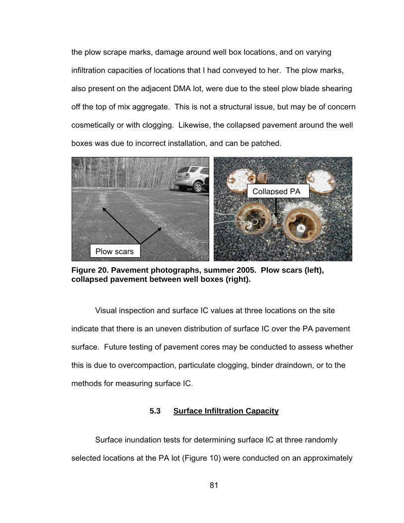
the plow scrape marks, damage around well box locations, and on varying
infiltration capacities of locations that I had conveyed to her. The plow marks,
also present on the adjacent DMA lot, were due to the steel plow blade shearing
off the top of mix aggregate. This is not a structural issue, but may be of concern
cosmetically or with clogging. Likewise, the collapsed pavement around the well
boxes was due to incorrect installation, and can be patched.
Figure 20. Pavement photographs, summer 200collapsed pavement between well boxes (right)
Visual inspection and surface IC values at th
indicate that there is an uneven distribution of surfa
surface. Future testing of pavement cores may be
this is due to overcompaction, particulate clogging,
methods for measuring surface IC.
5.3 Surface Infiltration C
Surface inundation tests for determining sur
selected locations at the PA lot (Figure 10) were co
81
Collapsed PA
Plow scars
5. Plow scars (left), .
ree locations on the site
ce IC over the PA pavement
conducted to assess whether
binder draindown, or to the
apacity
face IC at three randomly
nducted on an approximately

monthly basis throughout late 2004, 2005, and 2006 (Appendix D, Table 16).
Figure 21 includes a time series and box plot of surface IC. All plotted values
have been corrected for leakage.
0
500
1000
1500
2000
10/1/04 4/1/05 10/1/05 4/1/06 10/1/06Date
Sur
face
IC (i
n/hr
) oo
o Pt A CorrectedPt B CorrectedPt C Corrected
;
840
20838
1343
597
147
1838
1451
391
0
500
1000
1500
2000
A B CPoint
Figure 21. Surface IC time series (left) and box plot (right).
Point A is a fast-infiltrating location in the south corner of the lot. It is on
pavement placed as pull 1 during construction. Despite significant fluctuations in
surface IC for Point A during the monitored time period, starting and ending
values were roughly equivalent. The most significant change occurred in the
2005 summer, as IC dropped from 1,800 in/hr (May) to a minimum of 840 in/hr
(November). The trend appeared to be unrelated to the type of seal used at the
base of the cylinder. IC rebounded during the late-fall 2005 and has leveled off
at approximately 1,000 in/hr.
Point B is a medium- to high-infiltrating location immediately northwest of
Well 5m/5d. It is on pavement placed as pull 3 during construction. As with
Point A, there were significant fluctuations in readings throughout the time period.
The trend followed that of Point A. Point B also witnessed a steep decline in IC
82

over the same time period (summer 2004). Point B IC values recovered during
the winter, and have since leveled off at approximately 450 in/hr.
Point C has been and continues to be a low-infiltrating location relative to
Points A and B. It is situated behind the ‘out’ arrow at the exit from the parking
lot, and is located on pavement placed as pull 5 during construction. The initially-
low surface IC at Point C is likely due to lower air void content and lower
permeability of the pavement at this location. This may have been caused by
higher temperature (190°F) during breakdown compaction than those for Points
B and C (170°F and 160°F) in previous pulls. In-place properties have not yet
been characterized for this location.
Like Points A and B, IC for Point C dropped significantly during summer
2005. However, the IC has leveled off since June, 2005 and is approximately 50
in/hr via the SIT method (corrected). Excessive leakage led to the decision to
verify SIT data with double ring infiltrometer (DRI) test data.
A DRI test adapted to permeable pavements (Bean 2004) was conducted
for Point C on October 2 and November 10, 2006 to address potentially
misleading IC readings due to high leakage observed during the SIT. The
constant head DRI test, which requires only 1 to 2 inches of standing water on
the pavement, had neglible leakage. The use of the outer ring accounted for any
lateral leakage from the inner ring. Mean IC was measured at 14 in/hr on
October 2 and at 35 in/hr on November 10, 2006. The SIT gave 230 in/hr
(uncorrected) and 57 in/hr (corrected) for the October 2 test. Location C was not
tested via the SIT on November 10.
83

Group means of corrected surface IC values were contrasted in order to
test whether a significant difference existed between locations and between
locations by season (Table 4). The relatively large sample sets (n =19, 19, 16)
for locations A, B, and C for all dates allowed for a meaningful contrast between
group means at 95% confidence. Each location was found to be significantly
different from each other (A > B > C). Locations A, B, and C were then grouped
by season (winter/spring and summer/fall), and contrasted with the equivalent
season in consecutive years (e.g. winter/spring 2004-2005 with winter/spring
2005-2006). Of the six seasonal contrasts, only two were significantly different.
Both Locations B and C dropped significantly during winter/spring from 2005 to
2006. For locations B and C during consecutive winter/spring periods, the group
means dropped from 1,250 in/hr to 600 in/hr, and from 340 in/hr to 150 in/hr,
respectively.
Table 4. Surface IC statistics grouped by location and by location/season.
1 2 1 2 1 2 1 2 1 2 1 2Mean 1319 739 185 1587 1278 1248 592 341 150 1173 1147 464 467 45 60SD 320 381 133 238 390 156 86 31 43 291 210 216 45 10 19St. Err. 73 87 33 97 195 64 43 12 22 145 94 108 20 6 11Hi 95% 1473 923 256 1837 1898 1412 729 373 218 1635 1408 808 523 71 106Lo 95% 1165 556 114 1337 657 1085 455 308 81 710 885 120 411 20 14n 19 19 16 6 4 6 4 6 4 4 5 4 5 3 3Sig diff. yes yes yes - no - yes - yes - no - no - noYear 1: 2004-2005 (Winter/Spring), 2005 (Spring/Summer).Year 2: 2005-2006 (Winter/Spring), 2006 (Spring/Summer).SD - Standard Deviation; Hi 95% - Upper 95% CI; Lo 95% - Lower 95% CI; n - number of samples.Significant difference at 95%.
Location A Location B Location CWinter-Spring Summer-FallLocation
Stat Location A Location B Location CA B C
The observed fluctuations in IC data may be due to differential compaction
between locations, introduction of particulates, draindown of asphalt binder,
and/or the test methodology. Clogging of air voids in PA due to particulates has
historically been a prime cause of surface IC decreases over time (Ferguson
84

2005). It is not clear if this is the case at this site. UNH Grounds & Roads
maintenance trucks have not been given any directives regarding plowing,
sanding, and salting practices. As a result, the PA lot has been treated the same
as the other DMA parking lots on campus. This “worst case” maintenance
scenario means that after a snow event, the site is cleared of snow with heavy
steel plow blades, and then a sand and salt mixture is applied. It has been
consistently observed that application of the sand-salt mixture is uneven and
excessive (Figure 22).
Less residual salt-sand mix on DMA lot
Clumped salt-sand mix on PA lot
Figure 22. Residual sand and salt mix on PA lot, winter 2005. Clumped mix (top) and close up of mix (bottom).
Based on laboratory analysis of the UNH Grounds and Roads salt-sand
mixture, sand is only 9.6% of the mixture by mass (refer to Chloride Mass
Balance for methodology and results). Based on the 347 lb of total chloride
mass in the PA effluent calculated from 7/1/05 to 6/30/06, total mixture mass was
620 lb. At 9.6 % by mass of the mixture, sand application was calculated at 60
lb. Much of this was localized deposition and may not have been deposited in
the IC testing locations.
85

There were other observed sources of particulates on the PA pavement.
Plowing over the past two winters has abraded several strips of pavements,
effectively shearing off aggregate surfaces (Figure 20). These aggregates have
been further fragmented, and have accumulated in the void spaces. A close up
photograph captures the contrast between the plow-abraded pavement and
unaffected areas (Figure 23, top left). In August, 2006 a pile of bark mulch was
deposited from an unknown source on a portion of the pavement near Point C
(Figure 23, top right). Another source of particulates, and one that is unique to
the UNH site, is the residual paint and material from the DMA speed bump.
Evidence of this material is found in low spots adjacent to the speed bump
(Figure 23, bottom).
Another possible cause of decreased IC values since construction may be
binder draindown. IC values dropped substantially starting in June 2005 after the
first intense heat of the season. This may indicate draindown of asphalt binder.
In this scenario, asphalt binder could be mobilized when increased heat lowers
its viscosity, thereby facilitating “draindown” into the lower portion of the
pavement. The increased binder in the lower layer, and inclusion of sediments
with this binder, could eventually clog the pore spaces, and impede the
downward percolation of water (Ferguson 2005). IC values dropped substantially
at all three locations during the 2005 summer months, and then stabilized by
October 2005. These observations are consistent with a high temperature-driven
binder draindown issue as described. However, the increased surface IC values
observed at Points A and B since then indicate that this may not be occurring in
86

Figure 23. Other observed particulate sources; plow-abraded PA aggregate (top left), bark mulch (top right), and speed bump material (bottom).
87

those locations. In the future, it is recommended that the pavement be cored in
several locations, sliced transversely several times, and then each section
analyzed for binder content and/or air void content to determine if draindown is
occurring.
The SIT methodology has been problematic due to difficulties from an
inadequate seal at the base of the stainless steel cylinder. This has resulted in
sometimes substantial lateral leakage of water from the test cylinder, and
consequent false high IC values. For moderate to high IC locations (Points A
and B), the leakage from the base of the surface inundation device was very
limited. For low IC Point C, it was more difficult to adequately seal the base, and
consequently leakage was significant.
Another potential factor in the SIT methodology that could impact IC is
changes in water viscosity due to temperature fluctuations. If water at the
freezing point were used, then the IC value could be expected to be smaller than
that of water at room temperature by a factor of 1.82 (Mays 2001). Temperature
effects were addressed by always using room temperature water. Seasonal
temperature-related viscosity effects were not observed in the IC data.
5.4 Frost Depth
Frost depth data were taken from a centrally located groundwater well (5s)
in the PA pavement for short periods of winters 2005 and 2006. Well 5s is a 4
feet deep, 1-inch diameter, schedule 40 PVC groundwater monitoring well. It is
fully screened and is typically dry.
88

Frost depths during the month of March 2005 varied from 0 to 1 foot
(Figure 24). Most of the non-zero frost depths occurred during or after cold
periods, such as 0.5 foot depth (3/3/05) and 1.0 ft depth (3/11/05). The March
15, 2005 reading of 1.0 foot, however, followed 3 days of predominantly above
freezing daytime temperatures. Nighttime temperatures dropped below freezing
each of those nights. The last positive frost depth recorded for 2005 was on
March 6 (0.4 feet), after several days of above-freezing air temperatures.
0.0
0.5
1.0
1.5
2.03/1/05 3/8/05 3/15/05 3/22/05 3/29/05 4/5/05
Date
Fros
t Dep
th (f
t)
0
30
60
90
120
Tem
pera
ture
(°F)
Frost DepthAir TempFreezing Point
Figure 24. Frost depth and air temperature for March, 2005.
Frost depth data for January through March 2006 are plotted in Figure 25.
Freezing depth varied from a maximum of 0.8 feet (1/3/06) to a minimum of 0
feet at several times during the study period. Frost depth trends lagged behind
air temperature by a few days. A warm period from approximately January 15 to
February 15, 2006 witnessed no observed frost depth, while frost depth
increased to 0.7 feet after a few days (by 2/20/06) of freezing air temperatures.
89
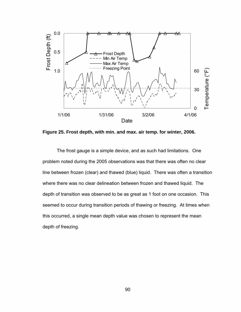
0.0
0.5
1.0
1.5
2.01/1/06 1/31/06 3/2/06 4/1/06
Date
Fros
t Dep
th (f
t)
0
30
60
90
120
Tem
pera
ture
(°F)
Frost DepthMin Air TempMax Air TempFreezing Point
Figure 25. Frost depth, with min. and max. air temp. for winter, 2006.
The frost gauge is a simple device, and as such had limitations. One
problem noted during the 2005 observations was that there was often no clear
line between frozen (clear) and thawed (blue) liquid. There was often a transition
where there was no clear delineation between frozen and thawed liquid. The
depth of transition was observed to be as great as 1 foot on one occasion. This
seemed to occur during transition periods of thawing or freezing. At times when
this occurred, a single mean depth value was chosen to represent the mean
depth of freezing.
90

5.5 Water Balance
A water balance was conducted between precipitation and PA effluent for
the 18-month period from April 1, 2005 to September 30, 2006 (Table 5, Figure
26, Figure 27). Monthly precipitation varied substantially throughout the study
period. Peak monthly precipitation volumes were observed in October 2005
(40,000 gal) and May 2006 (55,000 gal). Minimum monthly precipitation volume
was observed in March 2006 (3,500 gal).
Table 5. Water balance between rainfall and PA effluent.
Precip Effluent Net Precip Effluent NetApril 2005 5.43 18,954 26,436 -7,482 0.7 18,954 26,436 -7,482May 2005 6.84 23,871 26,155 a -2,283 0.9 42,826 52,591 -9,765
June 2005 4.45 15,533 12,818 2,715 1.2 58,359 65,409 -7,050July 2005 2.27 7,924 1,319 6,605 6.0 66,283 66,728 -445
Aug. 2005 3.06 10,678 108 10,570 99 76,961 66,836 10,124Sept. 2005 2.51 8,762 86 8,675 102 85,723 66,923 18,800Oct. 2005 b 11.58 40,416 33,450 6,966 1.2 126,139 100,373 25,766Nov. 2005 5.35 18,676 12,344 6,332 1.5 144,815 112,717 32,098Dec. 2005 4.48 15,639 19,053 -3,413 0.8 160,455 131,770 28,685Jan. 2006 3.70 12,918 18,997 -6,079 0.7 173,373 150,767 22,606Feb. 2006 2.50 8,727 6,867 1,860 1.3 182,100 157,633 24,466Mar. 2006 1.00 3,491 4,613 -1,122 0.8 185,590 162,246 23,344April 2006 3.37 11,764 4,445 7,319 2.6 197,354 166,692 30,662May 2006 15.71 54,834 44,076 10,758 1.2 252,188 210,768 41,420
June 2006 c 8.85 30,894 25,030 5,864 1.2 283,082 235,798 47,284July 2006 4.28 14,938 3,374 11,564 4.4 298,020 239,172 58,848
Aug. 2006 4.11 14,347 3,455 10,893 4.2 312,367 242,627 69,741Sept. 2006 2.81 9,812 99 9,713 99 322,180 242,726 79,454
bFlow data from October 24 to November 1, 2005 was inadvertently lost due to a software error, and is not accounted for in the monthly and quarterly values. Precipitation from this period (2.02 in) is deducted from the monthly total for purposes of comparison.cFlow and precipitation data from June 26, 2006 to June 30, 2006 at the effluent monitoring site was lost due to a power outage. The 0.14 inches which fell during that period was added to the monthly total. No flow was added since this small rainfall was unlikely to trigger flow.
Precip:Eff Ratio
Cumulative Volume (gal)Time period Precip (in)
aA power outage occurred during a storm event from May 23 to May 24. Effluent flow was computed as the average of the starting and ending values.
Monthly Volume (gal)
91

0
20,000
40,000
60,000
80,000
100,000
April 2
005
May 20
05
June
2005
July
2005
Aug. 2
005
Sept. 2
005
Oct. 20
05
Nov. 2
005
Dec. 2
005
Jan.
2006
Feb. 2
006
March 2
006
April 2
006
May 20
06
June
2006
July
2006
Aug. 2
006
Sept. 2
006
Date
Vol
(gal
)
-48,000
-36,000
-24,000
-12,000
0
12,000
Net
Vol
(gal
)
Monthly PrecipMonthly Effluent
-----------------------------------------------------------------------------------------------------------------------------------------
Monthly Net Inflow
0.7 0.9 1.26.0
99 102
1.2 1.5 0.8 0.7 1.3 0.82.6 1.2 1.2
4.4 4.2
99
01
10
1001,000
Vol
Rat
io
Figure 26. Monthly water balance and ratio of precipitation to effluent.
-50,000
0
50,000
100,000
150,000
200,000
250,000
300,000
350,000
4/1/05 7/1/05 9/30/05 12/30/05 4/1/06 7/1/06 9/30/06Date
Cum
. Vol
(gal
)_
PrecipitationEffluentNet Inflow
Figure 27. Cumulative water balance.
92
Several factors affected the water balance between precipitation and PA
effluent: inflows included direct precipitation, snowmelt (delayed precipitation),
and groundwater (exfiltration); outflows included the PA effluent flow, infiltration
into the subgrade, evaporation, and precipitation lost to plowing. After snow
events, the lot was plowed and snow piled into snow banks on the edge of the
lot. Some of the snow eventually infiltrated into the system as snowmelt through
the crushed gravel perimeter drain. However, snow piled beyond the edges of
this 1.5 foot apron (beyond edge of pavement) eventually drained in the opposite
direction as snowmelt and did not contribute as an inflow. Due to the mild cold
periods and light snow pack, this effect was not considered significant.
Groundwater flow into and out of the PA porous media reservoir was
characterized by plotting groundwater elevations of two nested wells, Well 5m
and Well 5d over the study period (Figure 28). Well 5m is screened from 88.65 ft
MSL to 91.65 ft MSL, slightly above the base of the PA porous media reservoir
(91.2 ft MSL). Well 5d is screened lower, from 85.38 ft MSL to 90.38 ft MSL,
below the base. Since these two wells are nested, it was possible to determine
direction of groundwater flow given groundwater elevations for the two wells.
Whenever groundwater elevation was higher in Well 5m (higher screened
interval), flow was downwards. Conversely, higher groundwater in Well 5d
indicated upwards flow of groundwater. For groundwater to enter the porous
media reservoir from below (exfiltration), groundwater level in Well 5m had to be
at or above the base of the porous media reservoir. Based on these criteria,
exfiltration occurred from approximately 12/15/05 to 1/15/06. Infiltration of
93

standing water in the porous media reservoir occurred from approximately 4/1/05
to 6/1/05 and from 1/15/06 to 3/31/06.
90.5
90.6
90.7
90.890.9
91.0
91.1
91.2
91.3
91.491.5
4/1/05 7/1/05 9/30/05 12/30/05 3/31/06 6/30/06 9/29/06Date
GW
Ele
v (ft
MS
L)
-0.1
0.0
0.1
0.2
0.3
0.4
0.5
0.6
0.7
0.8
Diff
in G
W E
lev
(ft)
Well 5mWell 5dDiff (5m - 5d)
Bottom of Bed
GW moving upwards
GW moving downwards
GW intosystem
GW out of system
Figure 28. Groundwater elevations for Wells 5m and 5d, and differences in elevation as indicator of infiltration or exfiltration.
Pronounced trends were observed during both summers. There were
extremely high ratios of precipitation to PA effluent during July, August, and
September of both 2005 (6.0, 99, 102) and 2006 (4.4, 4.2, 99). This suggests
that the majority of the precipitation either infiltrated into the subgrade or
evaporated during these times. Evaporation of groundwater upward through the
pavement is unlikely to be significant, since the capillary effect would not allow
groundwater or any standing water to be carried to the surface due to porous
media construction. Groundwater was below the base of the porous media
reservoir during summer months. Therefore, evaporation is primarily from the
residual water in the top few inches. The use of single-sized ¾-inch crushed
94

gravel for the bottom 24 inches of the porous media reservoir and for 4 inches
immediately below the pavement would not allow water to be transported upward
through the large pore spaces due to capillary effect (Mays 2001). During these
warm summer periods, high air temperatures and high pavement temperatures
may have contributed to increased evaporation of precipitation intercepted in the
pavement layer. Additionally, precipitation was slightly low to average during
these months, and would require less solar energy to evaporate. Although not
tested, evaporation could potentially be enhanced due to air flow through the
system. This effect is not believed to be significant, however, due to the small
underdrain pipe diameter (6 inches) and to large head losses likely to be incurred
in the compacted, well-graded bank run gravel layer.
During months with the greatest precipitation (10/05, 5/06, 6/06),
precipitation exceeded PA effluent. Much of this excess precipitation was
infiltrated. Well data supports this, since groundwater movement was
downwards during these times. In 4/05 and 5/05, and again in 12/05 and 1/06,
PA effluent exceeded precipitation. Some of this excess PA effluent may have
been due to exfiltrated groundwater (into the PA porous media reservoir from
below). This is supported by groundwater well data, wherein exfiltration occurred
from approximately 12/15/05 to 1/15/06.
Cumulative precipitation increased at a rate greater than cumulative PA
effluent for most of the study period. Cumulative PA effluent was greater than
cumulative precipitation from April 2005 until late July 2005, reflecting the
delayed effects of snowmelt and low precipitation relative to PA effluent.
95

Cumulative precipitation then exceeded PA effluent until the end of the study
period. By 9/30/06, precipitation volume totaled 322,000 gallons, and PA effluent
volume totaled 243,000 gallons, resulting in a net cumulative inflow volume of
79,000 gallons (22.8 inches). 75% of total precipitation flowed out of the system
through the underdrain over the study period. 25% of precipitation was infiltrated
into the subgrade. Infiltration may have been more significant if the bottom of the
porous media reservoir were flat. This would have provided a greater surface
area over which water could infiltrate into the subgrade.
5.6 Chloride Mass Balance
A mass balance for chloride was performed between salt application by
UNH Grounds & Roads and the PA effluent from 7/1/05 to 6/30/06. D-Box
chloride mass was also calculated. This one-year time period was selected
because the start and end (summer) should be the time of lowest SC
concentration, as the application of salt occurred during winter.
5.6.1 Chloride Mass Applied by UNH Grounds & Roads
Table 6 summarizes documented salt application dates by UNH Grounds
& Roads. 21 salting events were documented; the first was conducted on
11/24/05, and the last on 2/26/06. Based on the number of storm events, total
chloride mass applied at the PA lot was estimated to be 508 lb (Table 7). Total
chloride mass applied to an equivalent area on the West Edge Lot was
calculated to be 431 lb.
96

Table 6. UNH Grounds & Roads salt application data.
Date Depth (ft)
Precip (in)
Temp < 32°F
1 11/24/05 ALA (6) 11/24/05 0.07 0.41 yes yes2 12/5/05 DAS (1.5) 12/5/06 0.05 0.00 yes yes3 12/9/05 DAS (2.5) - - 0.58 yes yes4 12/10/05 JKF (14) 12/9/05 0.92 0.09 yes yes5 12/16/05 DAS (4); ALA (7.5) - - 1.68 yes yes6 12/24/05 DAS (2) - - 0.01 no no7 12/27/05 DAS (4.5) - - 1.37 yes yes8 12/31/05 ALA (2) - - 0.01 yes yes9 1/1/06 DAS (4) 1/1/06 0.11 0.06 yes yes
10 1/3/06 DAS (3) - - 0.00 yes no11 1/5/06 DAS (3) 1/5/06 0.29 0.25 yes yes
12 1/15/06MAE (4.5); FD (3); SPC (3); CMB (3); KAS (3); JAM (3)
- - 0.78 yes yes
13 1/17/06 ALA (5) - - 0.34 yes yes14 1/24/06 JKF (5.5) 1/23/06 0.46 0.61 yes yes15 1/25/06 JRB (6); JAM (9.5) - - 0.26 yes yes16 1/30/06 DAS (1) - - 0.52 yes yes17 1/31/06 ALA (4) - - 0.01 yes yes18 2/12/06 DAS (5) 2/12/06 0.42 1.33 yes yes19 2/23/06 JKF (2) - - 0.09 yes yes20 2/25/06 DAS (3) - - 0.22 yes yes21 2/26/06 JKF (12.5) 2/25/06 0.42 0.03 yes yes
Time spent on snow removal or salting West Edge Lot based on timesheet activity code SNOMECH1. Each time SNOMECH1 billed, assume salt was
Salt was often applied before forecasted storm events. Some forecasts never actually resulted in snow or freezing rain.
Snow depth from NOAA Durham gauge. Temp and heated rain gauge data from UNH Weather Station. If temp < 32°F before, during, or after the event, then assumed that snow or frozen rain could result. Sometimes precip from previous day(s) was added if maintenance work was delayed (e.g. holidays).
Event No.
Date of Salt App.
NOAA SnowTime (initials, hours)
UNHWS Data Snow or Freezing
Rain?
5.6.2 Chloride Mass at D-Box and PA effluent from SC Regression Equation
A time series plot of D-Box and PA effluent SC readings is included in Figure 29.
Since salt application is the principal variable for SC readings, the winter period
is magnified, and salt application dates are shown. Significant spikes in SC for
97

the D-Box started in late November, increased in magnitude into late December,
and recurred with decreasing magnitude and frequency into April. Peak D-Box
SC occurred in late-December. A lag between D-Box SC and PA effluent SC
was evident in the time series. PA effluent SC peaked in mid-January, and
continued at elevated levels into May. SC peaks for the D-Box were much higher
and of shorter duration than for the PA effluent.
98

1
10
100
1,000
10,000
100,000
7/1/05 9/30/05 12/30/05 3/31/06 6/30/06Date
SC
(uS
/cm
)
D-Box Effluent
100
1,000
10,000
100,000
11/24/05 12/8/05 12/22/05 1/5/06 1/19/06 2/2/06 2/16/06 3/2/06Date
SC
(uS
/cm
)
Salt Applied D-Box Effluent
Figure 29. SC time series for D-Box and PA effluent from 7/1/05 to 6/30/06 (top) and for the winter with salt application events (bottom).
Chloride mass loading calculations and assumptions are presented in
Table 7. Chloride mass balance data from SC regression between D-Box and
PA effluent is presented in Table 8. Chloride mass was calculated from flow-
weighted SC readings through a site-specific regression equation. Figure 30 and
Figure 31 show monthly and cumulative chloride mass balance plots.
99

Table 7. Chloride mass based on lineal loading by tarp experiment. Parameter Value Units Basis
Salt application events 21 - UNH G&R Passes per storm event 2 pass UNH G&R; photosMass Cl per lineal foot ( from tarp) 0.11 lb UNH lab resultLength of each PA lot pass (110 ft) 0.021 miles measuredPercent Cl in mix (by mass) 56% % UNH lab resultPA mass Cl per pass 12.1 lb calculatedPA mass Cl per storm event 24.3 lb calculated
PA seasonal mass Cl 509 lb calculatedWest Edge lane-miles 1.27 miles construction drawingsWest Edge seasonal mass Cl 31,050 lb calculated
West Edge seasonal mass Cl/ 72 431 lb calculatedAssumed consistent distribution of Cl per lane-mile.Assumed that all mix spread was captured by tarp.
Table 8. Chloride mass balance from 7/1/05 to 6/30/06.
Precip DX Eff DX Eff DX Eff App DX Eff Net App DX Eff NetJuly 2005 7924 3498 1319 130 581 16 169 0 0.5 1.9 -1.4 0 0.5 2 -1.4
Aug. 2005 10678 3360 108 116 447 11 124 0 0.3 0.1 0.2 0 0.8 2 -1.2Sep. 2005 8762 5621 86 18 360 0 94 0 0.0 0.1 -0.1 0 0.8 2 -1.3Oct. 2005 a 40416 44940 33450 57 183 0 34 0 0 9.5 -9.5 0 1 12 -11Nov. 2005 18676 34513 12344 805 241 246 53 24 71 5.5 65 24 72 17 55Dec. 2005 15639 17562 19053 2101 489 688 138 169 101 22 79 194 172 39 133Jan. 2006 12918 41319 18997 1981 3174 647 1054 218 223 167 56 411 396 206 189Feb. 2006 8727 19557 6867 1021 2316 320 761 97 52 44 8.5 508 448 250 198Mar. 2006 3491 6020 4613 813 2027 249 663 0 12 26 -13 508 460 275 185April 2006 11764 14364 4450 249 1873 56 610 0 6.8 23 -16 508 467 298 169May 2006 54834 74744 44076 150 316 23 79 0 14 29 -15 508 481 327 154
June 2006 b 30894 72504 25031 262 364 61 96 0 37 20 17 508 518 347 171SC and Cl values are monthly flow-weighted mean concentrations.App - Chloride mass applied by UNH Grounds & Roads, estimated.Net - Difference between D-Box (DX) and effluent mass Cl.aPrecipitation and flow data from 10/24/05 to 11/1/05 was inadvertently lost, and is not accounted for in the table.bFlow and precipitation data from 6/26/06 to 6/30/06 at the effluent monitoring site was lost due to a power outage.
Inc Mass Cl (lb) Cum Mass Cl (lb)Month Volume (gal) SC (uS/cm) Cl (mg/L)
100

0
100
200
300
400
July
2005
Aug. 2
005
Sep. 2
005
Oct. 20
05
Nov. 2
005
Dec. 2
005
Jan.
2006
Feb. 2
006
Mar. 20
06
April 2
006
May 20
06
June
2006
Date
Cl M
ass
(lb)
-300
-200
-100
0
100
Net
Cl M
ass
(lb)
Applied Cl MassD-Box Cl MassEffluent Cl Mass
Monthly Net Cl Mass
Figure 30. Monthly chloride mass balance from 7/1/05 to 6/30/06.
-100
0
100
200
300
400
500
7/1/05 9/30/05 12/30/05 3/31/06 6/30/06Date
Cum
. Cl M
ass
(lb)
Applied Cl MassD-Box Cl MassEffluent Cl MassNet Cl Mass
Figure 31. Cumulative chloride mass balance from 7/01/05 to 6/30/06.
Applied chloride mass closely matches the pattern and magnitude of D-
Box chloride mass, as would be expected. Both applied and D-Box monthly
101

chloride mass increased from zero starting in October to peak monthly values of
101 and 223 lb in December and January, respectively. They then dropped to
neglible levels by March.
PA effluent chloride mass first appeared in significant quantities in
October. Chloride mass increased gradually during November and December,
and peaked in January (167 lb). January PA effluent mass was almost half of the
annual total (347 lb). PA effluent mass decreased substantially in February (44
lb) and leveled off to approximately 25 lb per month through June 2006. While
not verified with field experiments, this lagged effect of chloride export from the
PA effluent may be explained by slow bleeding out of salt trapped in the upper
unsaturated portion of the porous media filter by infiltrated precipitation. May and
June had extremely high rainfall depths and may have “flushed out” the chloride
mass left from salt applications earlier in the winter.
The lag in chloride mass from applied salt and D-Box to PA effluent was
similar to the SC pattern observed in the time series plot, as would be expected.
The chloride mass centroid for D-Box (259 lb) occurred in December and for PA
effluent (174 lb) occurred in January. Net monthly export was increasingly
negative through December, and then became highly positive in January, the
peak month. Net monthly export decreased gradually, and again became
negative by June. Net import of chloride increased through December, and
decreased to become slightly negative by the end of May.
For a conservative pollutant such as chloride that does not bind easily to
soil particles or pavement under common environmental conditions, D-Box
102

(influent) and PA effluent mass should balance, assuming there are no other
sources or sinks. It has been speculated that salting was heavier at the PA site
due to the residual salt crystals frequently seen at the PA lot (Figure 22). After
sand/ salt application, salt granules could frequently be seen for days after all
snow and ice had melted through the pavement. However, UNH Grounds and
Roads personnel claimed that this site was treated the same as other parking lot
areas (Appendix F). Furthermore, the persistence of salt granules on the PA lot
may be explained by the lack of prolonged contact with water. Water infiltrates
rapidly upon contacting PA and does not allow for dissolution of salt crystals,
unlike DMA pavement where puddles (or at least standing water) often form.
5.7 Hydraulic Efficiency
The hydrograph and hydraulic performance summary table for the 4/20/05
event are presented in Figure 32 and Table 9, respectively. The remaining storm
event hydrographs (Figure 49 through Figure 59) and hydraulic performance
tables (Table 19 through Table 29) are included in Appendix D. A summary of
the important precipitation (influent) and PA effluent hydraulic performance
parameters for 12 storm events is included in Table 10. This table presents
summary statistics on precipitation, peak flow reduction, and PA effluent lag for
each storm event. Precipitation, D-Box flow, and PA effluent flow are plotted
versus storm event time for each of the 12 storm events. For all statistics
presented, precipitation is compared to PA effluent. D-Box flow is presented for
comparative purposes only.
103

104
0
5
10
15
20
0 500 1,000Time (min)
Flow
(gpm
1,500
)
0
0.02
0.04
0.06
0.08
5-M
in. P
reci
p (in
0.1
)
D-Box FlowEffluent FlowPrecip
Peak
Precip. Centroid
Effluent Peak Flow
Effluent Centroid at 2,690 min.
D-Box Centroid
Parameter Preci
Figure 32. Hydrograph and hyetograph of the 4/20/05 event. Table 9. Hydraulic performance summary of the 4/20/05 event.
p D-Box Effluentantecedent dry period (days) 17.2 - -start time (date/time) 4/20/05 20:05 - -duration (min) 480 515 4,545depth (in) 0.58 0.66 0.58storm volume (gal) 2,025 2,299 2,025volume centroid (gal) 1,012 1,150 1,012time of centroid (min) 220 265 2,690lag time (min) - 45 2,470kL - - 12.2peak intensity (in/5-min) 0.04 - -peak flow (gpm) 26 11 0.93time at peak flow (min) 5 15 1,585Kp - - 0.04D-Box flow presented herein is 1/72 of actual D-Box flow in order to compare flow statistics from equivalent watershed area as the PA (effluent).

Storm Duration
(min)
Prior Rainfalla
(day)
Storm Depth
(in)
Peak Intensity (in/hr)
Storm Volume
(gal)
Peak Precip. (gpm)
Peak Eff Flow (gpm)
kpPrecip.
Centroid (min)
Effluent Centroid
(min)
Lag time (min)
kL
1 4/20/05 480 17.2 0.58 0.04 2,025 26 0.93 0.04 220 2,690 2,470 12.22 5/7/05 965 4.1 0.63 0.01 2,199 6.5 1.3 0.20 410 1,855 1,445 4.53 5/21/05 1150 6.0 0.91 0.02 3,177 13 1.96 0.15 460 1,780 1,320 3.94 8/12/05 765 10.8 0.51 0.08 1,780 52.1 0.3 0.01 360 2,985 2,625 8.35 9/15/05 630 10.7 0.89 0.18 3,107 117.3 0.2 0.00 545 1,500 955 2.86 10/8/05 1865 8.3 5.00 0.10 17,453 65.2 23.5 0.36 965 1,480 515 1.57 11/30/05 805 5.6 0.69 0.03 2,409 19.5 2.8 0.14 535 1,100 565 2.18 12/16/05 625 5.3 1.38 0.06 4,817 39.1 4.2 0.11 425 915 490 2.29 1/11/06 300 6.2 0.46 0.04 1,606 32.6 1.8 0.06 185 1,700 1,515 9.210 3/13/06 1415 15.3 0.92 0.04 3,211 26.1 4.2 0.16 660 1,855 1,195 2.811 5/1/06 2130 7.6 2.99 0.06 10,437 39.1 4.2 0.11 1,005 1,915 910 1.912 6/1/06 1035 10.9 2.46 0.41 8,587 267.2 14 0.05 320 1,100 1,195 3.4
Minimum 300 4.1 0.46 0.01 1,606 6.5 0.20 0.00 185 915 490 1.525th Quartile 629 5.9 0.62 0.04 2,156 24.4 1.21 0.05 350 1,385 824 2.1Median 885 8.0 0.90 0.05 3,142 35.9 2.38 0.11 443 1,740 1,195 3.175th Quartile 1,216 10.8 1.65 0.09 5,760 55.4 4.20 0.15 574 1,870 1,463 5.5Maximum 2,130 17.2 5.00 0.41 17,453 267.2 23.50 0.36 1,005 2,985 2,625 12.2Average 1,014 9.0 1.45 0.09 5,067 58.6 4.95 0.12 508 1,740 1,267 4.6St. Dev. 552 4.1 1.37 0.11 4,795 71.9 6.91 0.10 260 613 693 3.4
kp, peak reduction coefficient, the ratio of peak effluent flow to peak rate of precipitation integrated over watershed area.kL, lag coefficient, the ratio of the effluent centroid to the precipitation centroid.
aPrior rainfall calculated as the time in days of antecedent dryness since a minumum 0.1 inch storm event, using the UNH Weather Station gauge. All precipitation falling within 6 hours counts as the same storm event.
Effluent Delay
DateEvent No.
Precipitation Peak Flow Reduction
Table 10. Hydraulic performance summary for 12 storm events.
105
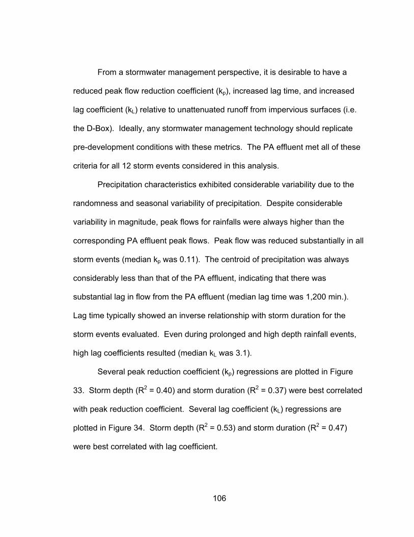
From a stormwater management perspective, it is desirable to have a
reduced peak flow reduction coefficient (kp), increased lag time, and increased
lag coefficient (kL) relative to unattenuated runoff from impervious surfaces (i.e.
the D-Box). Ideally, any stormwater management technology should replicate
pre-development conditions with these metrics. The PA effluent met all of these
criteria for all 12 storm events considered in this analysis.
Precipitation characteristics exhibited considerable variability due to the
randomness and seasonal variability of precipitation. Despite considerable
variability in magnitude, peak flows for rainfalls were always higher than the
corresponding PA effluent peak flows. Peak flow was reduced substantially in all
storm events (median kp was 0.11). The centroid of precipitation was always
considerably less than that of the PA effluent, indicating that there was
substantial lag in flow from the PA effluent (median lag time was 1,200 min.).
Lag time typically showed an inverse relationship with storm duration for the
storm events evaluated. Even during prolonged and high depth rainfall events,
high lag coefficients resulted (median kL was 3.1).
Several peak reduction coefficient (kp) regressions are plotted in Figure
33. Storm depth (R2 = 0.40) and storm duration (R2 = 0.37) were best correlated
with peak reduction coefficient. Several lag coefficient (kL) regressions are
plotted in Figure 34. Storm depth (R2 = 0.53) and storm duration (R2 = 0.47)
were best correlated with lag coefficient.
106

y = 8.67x + 0.45R2 = 0.40
0.1
1
10
0.001 0.01 0.1 1
Dep
th (i
n)
y = 0.0242x-0.297
R2 = 0.2206
0
0.1
0.2
0.3
0.4
0.5
0.001 0.01 0.1 1kp
Pea
k i (
in/5
-min
)
y = -0.95x2 + 3.68x + 0.61R2 = 0.37
0
1
2
3
0.001 0.01 0.1 1
Dur
. X 1
03 (min
)
y = 99.64x2 - 46.80x + 12.15R2 = 0.20
0
6
12
18
24
0.001 0.01 0.1 1kp
Prio
r Rai
n (d
ays)
Figure 33. Peak reduction coefficient (kp) regression plots.
y = 3.1093x-0.8242
R2 = 0.5289
0.1
1
10
0 3 6 9 12
Dep
th (i
n)
y = -0.001x2 + 0.011x + 0.079
R2 = 0.045
0.01
0.1
1
0 3 6 9 12kL
Pea
k i (
in/5
-min
)
y = 1.8508x-0.5712
R2 = 0.4689
0
1
2
3
0 3 6 9 12
Dur
. X 1
03 (min
)
y = 0.1712x2 - 1.7286x + 11.462
R2 = 0.323
0
6
12
18
24
0 3 6 9 12kL
Prio
r Rai
n (d
ays)
Figure 34. Lag coefficient (kL) regression plots.
107

5.8 Real-Time Water Quality Performance
EMC values of real-time water quality parameters (SC, DO, pH, and
temperature) for 12 storm events are presented in Table 11. The storm events in
this section are the same as used in the hydraulic performance analysis. Box
plots of these data are presented in Figure 35. Time series and box plots of
these parameters for the individual storm events are included in Appendix C.
Table 11. Real time water quality EMC values for 12 storm events.
D-Box Effluent D-Box Effluent D-Box Effluent D-Box Effluent
1 4/20/05 316 2,932 10.2 8.6 6.0 7.1 54 492 5/7/05 359 1,855 11.2 9.4 6.1 7.2 49 513 5/21/05 194 1,087 11.6 8.1 6.2 7.2 52 544 8/12/05 143 390 7.3 7.3 5.1 7.2 72 765 9/15/05 14 360 7.7 5.1 5.4 7.2 73 716 10/8/05 9 210 9.1 7.8 5.9 6.7 63 677 11/30/05 436 634 9.8 9.7 6.3 7.0 52 508 12/16/05 1,835 643 9.7 11.1 6.2 7.0 34 449 1/12/06 821 3,288 13.0 11.0 6.2 7.0 36 41
10 3/13/06 330 1,999 11.8 11.8 6.4 6.9 45 4111 5/2/06 186 481 10.0 9.2 6.0 7.2 51 5312 6/1/06 337 279 6.2 8.6 6.1 6.9 71 62
pH Temp. (deg. F)Storm Event
Event No.
SC (uS/cm) DO (mg/L)
A paired D-Box/PA effluent contrast of EMCs for SC, DO, pH, and temp
for 12 storm events was conducted via the Student t-test using JMP 3.0 statistical
software (Table 12). All distributions were normal, which allowed for this
parametric test. The confidence level was 95%.
108

9210323
639
1835
3288
0
1000
2000
3000
D-Box Effluent
SC
(uS
/cm
)
6.25.1
9.98.9
13.011.8
4
6
8
10
12
14
D-Box Effluent
DO
(mg/
L)
5.1
6.7
6.1
7.1
6.4
7.2
5.0
5.5
6.0
6.5
7.0
7.5
D-Box Effluent
pH
3441
52 52
7376
30
40
50
60
70
80
D-Box Effluent
Tem
p (°
F)
Figure 35. Box plots of real time water quality EMC values for 12 events. Table 12. Paired Student t-test on real time water quality EMC values.
EMC Parameter No. Paired Events
Mean D-Box
Mean Effluent
Mean Diff
% of Events Exporting p-value sig diff
SC (uS/cm) 12 415 1180 -765 83% 0.0358 yesDO (mg/L) 12 9.80 8.98 0.83 NA 0.1152 nopH 12 5.99 7.05 -1.06 NA <0.0001 yesTemp (deg F) 12 54.33 54.92 -0.59 NA 0.7038 no
109

Each of the real time water quality parameters are discussed in detail in
the following sections.
5.8.1 Specific Conductivity (SC)
Significant differences between D-Box and PA effluent were detected for
SC for the 12 storm events (p-value of 0.0358). SC was significantly higher in
the PA effluent (mean 1,180 uS/cm) than the D-Box (mean 415 uS/cm). There
was a net SC (chloride) export for 83% of events. The two events for which D-
Box SC was higher than PA effluent SC were 12/16/05 and 6/1/06. This may be
attributed to the timing of the events; it is likely that there was some residual salt
on the watershed before the event. Since there was observed to be a seasonal
time lag in peak SC at the PA effluent relative to D-Box SC, it can be explained
by noting that the chloride had not reached the PA effluent yet. The salt had not
fully infiltrated into the PA bed in significant quantities by this time. Additionally,
the salt must mix with the residual water below the underdrain in the porous
media reservoir.
During storm events, there were predictable patterns of SC observed
(Figure 36). D-Box SC dropped once flow began, and then gradually increased
back to the pre-storm level as flows dissipated. Conversely, PA effluent SC
increased rapidly once flow began, and then gradually decreased to pre-storm
levels as flow decreased.
110

-2000
0
2000
4000
0 500 1,000 1,500 2,000 2,500
SC
(uS
/cm
)
0
20
40
60
80
Flow
(gpm
)
Influent SCEffluent SCInfluent FlowEffluent Flow
D-box SC drops in response to d-box flow, then eventually returns to original value.
Effluent SC rises in response to effluent flow, then eventually returns to original value.
Figure 36. SC time series of D-Box and PA effluent for the 1/11/06 event.
5.8.2 Dissolved Oxygen (DO)
DO was not significantly different for the 12 storm events between D-Box
and PA effluent (p-value of 0.1152). PA effluent DO was usually slightly lower
than D-Box DO, with 66% of storm events reporting lower DO in the PA effluent
than at the D-Box. For a large 9 acre parking lot with a 36-inch discharge pipe
(D-Box) that creates significant turbulence and mixing, high DO is expected.
During the typical storm event, both D-Box and PA effluent DO spiked with
increasing flows, and then gradually decreased with dissipating flows.
5.8.3 pH
PA Effluent pH was consistently higher than that of the D-Box. This
difference was highly significant (p-value <0.0001). In all events, pH in the D-Box
111

increased to approximately 7 in the PA effluent. Median pH was 6.1 for the D-
Box and 7.1 for the PA effluent, respectively. The observed buffering effect is
likely due to percolation of acidic rainfall through the sand and gravel bed before
discharging in the PA effluent. During all storm events, both the D-Box and PA
effluent pH dropped in response to increased flow, then increased to pre-storm
levels as flow decreased.
5.8.4 Temperature
There was no significant temperature difference from D-Box to PA effluent
during the 12 storm events (p-value of 0.7038). Median temperatures observed
at the D-Box and PA effluent were 50.8 and 49.7 degrees F, respectively. PA
effluent temperatures in the storm event plots can be misleading during hot and
cold weather, especially when there’s little or no PA effluent flow, and when air
temperatures differ substantially from ground temperature. However, flow-
weighted values of temperature account for this issue.
112

5.9 Discrete Sample Water Quality Performance
The D-Box and PA effluent were sampled during the same 12 storm
events as for hydraulic performance and real time water quality analyses, and
then analyzed for several discrete water quality parameters. The DL in all
calculations was assumed to be zero. For samples collected late in storm event
where concentrations are typically lower and times greater between samples,
use of a half or full DL could create a deceptively high EMC value. Discrete
sample water quality EMC and RE values are presented in Table 13. A paired D-
Box/PA effluent contrast was conducted by using either the Students t-test for
normal distributions or a non-parametric test, Wilcoxon Rank Sums, with a
significance level of 95% (Table 14).
Median RE values are plotted in Figure 37. D-Box and PA effluent EMC
data are presented in treatment effect plots (Figure 38), box plots (Figure 39),
and PA effluent probability plots in independent, rank-ordered format (Figure 40).
Individual parameters are then discussed in their respective section.
Figure 37. Median RE values for discrete sample parameters.
-227
-113
33
100 99 96
-300-250-200-150-100
-500
50100150
Analyte
Med
ian
RE
(%)
Detection Limits:Cl: 0.1-25 mg/LTPH-D: 330-2,700 ug/LNO3-N: 0.05-0.5 mg/LTotal P-P: 0.01-0.3 mg/LTSS: 10-20 mg/LZn: 0.01-0.05 mg/L
Cl NO3-N Total P-P TPH-D ZnTSS
113

Table 13. Discrete sample water quality EMC and RE values for 12 events.
DX Eff RE DX Eff RE DX Eff RE DX Eff RE DX Eff RE DX Eff RE4/20/05 74 1,254 -1597 0.62 0.99 -59 NA NA NA 712 NA - 45 0.39 99 0.104 0.000 1005/7/05a 43 649 -1401 0 0.93 -273 NA NA NA 338 70 79 0 0 - 0 0 -5/21/05 NA NA NA 0.22 0.65 -202 0 0 - 221 NA NA 11 0 100 0.005 0 1008/13/05 10 25 -152 0.89 1.57 -77 0.16 0.04 72 1148 14 99 72 0 100 0.106 0.001 999/15/05 3 10 -219 0.26 1.67 -550 0.06 0.09 -49 710 0 100 12 0.53 95 0.035 0.003 9210/8/05 6 10 -78 0.25 0.71 -183 0.07 0.17 -147 573 0 100 6 6.6 -19 0.036 0.027 2511/30/05 NA NA NA 0.20 0.20 2 0.08 0.06 25 187 0 100 17 0 100 0.026 0 10012/16/05 NA NA NA 0.24 0.20 14 0.07 0.05 33 29 0 100 29 0 100 0.056 0.002 961/11/06 NA NA NA 0.35 0.49 -42 0.10 0.04 63 2178 185 92 52 5.00 90 0.035 0.046 -323/13/06 173 579 -235 0.27 0.40 -49 0.12 0.01 89 1338 0 100 74 0 100 0.051 0.004 915/1/06 NA NA NA 0.09 0.61 -581 0.15 0.07 52 1074 0 100 79 1.4 98 0.082 0 1006/1/06 NA NA NA 0.23 0.57 -150 0.22 0.37 -63 19204 0 100 188 20.3 89 0.062 0.038 40
DX: D-Box. Eff: Effluent. RE: Removal Efficiency (%).
TSS (mg/L) Zn (mg/L)
aNO3-N RE for the 5/7/05 event was calculated by using one half of the influent DL (0.5 mg/L) as the influent value (0.25 mg/L).
DateChloride (mg/L) TPH-D (ug/L)NO3-N (mg/L) Total P-P (mg/L)
114
Table 14. Paired Student t-test and Wilcoxon Rank Sum Test on discrete sample water quality parameters.
Student t-test
Wilc. Test
Cl (mg/L) 6 51.5 421.2 -369.7 100% 0.1120 - noNO3-N (mg/L) 12 0.30 0.75 -0.4475 83% 0.0032 - yesTotal P-P (mg/L) 10 0.10 0.09 0.013 30% 0.6499 - noTPH-D (ug/L) 10 2678 27 2651 0% - 0.002 yesTSS (mg/L) 12 48.75 2.85 45.90 8% - 0.002 yesZinc (mg/L) 12 0.050 0.010 0.04 8% - 0.005 yes
p-valuesig diff% of Events
ExportingMean Diff
Mean Effluent
Mean D-Box
No. Paired EventsEMC Parameter

0
500
1,000
1,500
0 500 1,000 1,500D-Box Cl (mg/L)
Effl
uent
Cl (
mg/
L)
Acute: 860 mg/L
Chronic: 230 mg/L
0
10
1,000
100,000
0 10 1,000 100,000D-Box TPH-D (ug/L)
Effl
uent
TP
H-D
(ug/
L)
0.0
0.5
1.0
1.5
2.0
0.0 0.5 1.0 1.5 2.0D-Box NO3-N (mg/L)
Effl
uent
NO
3-N
(mg/
L)
MCL: 10 mg/L
0
1
10
100
1,000
0 1 10 100 1,000D-Box TSS (mg/L)
Effl
uent
TS
S (m
g/L)
0.00
0.03
0.06
0.09
0.12
0.00 0.03 0.06 0.09 0.12D-Box Zn (mg/L)
Effl
uent
Zn
(mg/
L)
0.0
0.1
0.2
0.3
0.4
0.0 0.1 0.2 0.3 0.4D-Box Total P-P (mg/L)
Effl
uent
Tot
al P
-P (m
g/L)
Fed. River/ Stream Limit: 0.1 mg/L
115
Figure 38. Treatment effect plots of discrete sample EMC values.

0
0.200.24
0.630.89
1.67
0
1
10
N0 3
-N (m
g/L)
MCL: 10 mg/L
711
0
19,204
185
0
1
10
100
1000
10000
100000
Location
TPH
-D (u
g/L)
29
0 0
0.043
0.002
0.106
0.046
0.00
0.01
0.10
1.00
LocationZn
(mg/
L)
0 0
37
0.2
188
20.3
0
1
10
100
1000
Location
TSS
(mg/
L)
3.0
1027
302173
1,254
1
10
100
1000
10000
D-Box Effluent
Cl (
mg/
L) -------------------------Chronic: 230 mg/L
Acute: 860 mg/L----------------------------------------
0.00 0.00
0.090.05
0.22
0.37
0.0
0.1
0.2
0.3
0.4
Tota
l P-P
(mg/
L)
----------------------------------
Fed River/ Stream Limit: 0.1 mg/L
116
Figure 39. Box plots of discrete sample EMC values.

0%
100%
0 5000 10000 15000 20000
TPH-D (ug/L)
Per
cent
und
er
D-BoxEffluent
0%
100%
0.0 0.5 1.0 1.5NO3-N (mg/L)
D-BoxEffluent
MCL: 10 mg/L
0%
100%
0.00 0.05 0.10
Zn (mg/L)
D-BoxEffluent
0%
100%
0 500 1,000 1,500
Cl (mg/L)
Per
cent
und
er
D-BoxEffluentChronicAcute
0%
100%
0 50 100 150 200
TSS (mg/L)
D-BoxEffluent
0%
100%
0.0 0.1 0.2 0.3 0.4
Total P-P (mg/L)
D-BoxEffluent
Fed. Stream/ River Limit: 0.1 mg/L
Figure 40. PA effluent probability plots of discrete sample EMC values.
117

5.9.1 Chloride (Cl)
Chloride has been discussed in detail in previous sections (Chloride Mass
Balance, Real Time Water Quality Treatment Performance). Chloride EMC
values from direct analysis and from the SC regression equation of real time data
are compared for 6 storm events in Table 15. While values differ slightly, trends
in chloride by sample analysis and SC regression are similar for each of the
storm events. Chloride removal was highly negative for the six events evaluated,
meaning more chloride left the system than entered. In all cases, PA effluent
concentrations of chloride were substantially higher than D-Box concentrations.
EPA’s chronic chloride level of 230 mg/L was exceeded at the PA effluent for
three storm events (4/20/05, 5/07/05, and 3/13/06), and the EPA’s acute chloride
level (860 mg/L) was exceeded during the 4/20/05 event. Differences in chloride
concentration between the D-Box and PA effluent via the Student t-test were not
significant for analyzed samples, however (p-value of 0.1120).
Table 15. Chloride EMC values from analyzed samples and real time SC.
D-Box Effluent RE D-Box Effluent RE1 4/20/05 74 1,254 -1597% 79 971 -1129%2 5/7/05 43 649 -1401% 94 604 -542%4 8/13/05 10 25 -152% 20 104 -417%5 9/15/05 3 10 -219% 0 94 NA6 10/8/05 6 10 -78% 0 43 NA
10 3/13/06 173 579 -235% 84 653 -677%
Cl from Real Time SC EMCs (mg/L)Cl from Analysis (mg/L)Event No. Date
The chloride storm event performance values for chloride cannot be
extrapolated to time beyond the storm. Neither analyzed chloride EMC values
118

nor those calculated from SC EMC values capture longer term trends. The storm
event data for chloride cannot be used as a predictor for chloride mass balance
on an annual basis. While storm event chloride EMC values for PA effluent are
significantly higher than those for the D-Box, the 12-month chloride mass
balance indicated that D-Box significantly exceeded PA effluent.
5.9.2 Nitrate as Nitrogen (NO3-N)
PA water quality treatment for nitrate was in general poor during the 12
storm events evaluated. PA effluent concentrations of nitrate were greater than
D-Box for all but two storm events (11/30/05, 12/16/05), where little to no
treatment was observed. Median values of nitrate in the D-Box and PA effluent
were 0.24 mg/L and 0.63 mg/L, respectively. Median RE was -113%. While
nitrate treatment in general was not strong, it was observed to be consistent with
similar LID devices, such as the sand filter that has no vegetation growing on it,
or the manufactured infiltration unit at the UNH Stormwater Center principal field
site (CICEET 2006). D-Box and PA effluent nitrate concentrations were below
the EPA Maximum Contaminant Level (MCL) at 10 mg/L. PA effluent nitrate was
significantly higher than D-box nitrate via the Student t-test (p-value of 0.0032).
5.9.3 Total Phosphorus as Phosphorus (Total P-P)
Treatment performance for phosphorus for the 10 storm events was
modest. Median D-Box and PA effluent EMC values were 0.09 mg/L and 0.05
mg/L, respectively, resulted in RE of 33%. Only 25% of events witnessed
119

negative phosphorus removals (export). Statistical testing via the Student t-test
did not detect a significant difference between D-Box and PA effluent phosphorus
(p-value of 0.6499).
5.9.4 Total Petroleum Hydrocarbons as Diesel (TPH-D)
TPH-D treatment during 10 storm events was very strong. PA effluent
values were less than the DL in all storm events except three, where they were
still substantially less than those for the D-Box. TPH-D treatment performance
during the 6/1/06 storm event was exceptional, where the D-Box value was
19,204 ug/L, and the PA effluent was non-detect. Median TPH-D values in the
D-Box and PA effluent were 711 ug/L and 0 ug/L respectively, resulting in 100%
RE. Neither D-Box nor PA effluent TPH-D distributions were normally
distributed. There was a highly significant difference between D-Box and PA
effluent TPH-D values by the Wilcoxon Rank Sum Test (p-value of 0.002).
5.9.5 Total Suspended Solids (TSS)
Treatment performance of TSS was very strong for the 12 storm events
evaluated. Median D-Box and PA effluent values for TSS were 37 mg/L and 0.2
mg/L, respectively. Median RE was calculated at 99%. There was TSS removal
of at least 89% for all events except 10/08/05 (-19%). The October 8, 2005
storm event was exceptionally intense and storm depth was greater than 5
inches over several days. The June 1, 2006 storm event was the most intense
storm witnessed to date at the UNH Stormwater Center, resulting in high
120

mobilization of TSS (188 mg/L). While the PA effluent for this event (20.3 mg/L)
was the highest observed to date, it still resulted in 89% RE for TSS. The source
of TSS is likely fine subgrade materials (clays) that pass through the geotextile
filter fabric. Turbidity was also observed during an intense (maximum intensity
1.0 in/hr) 3.0 inch storm on October 11-12, 2006. Turbidity in the PA effluent
wasn’t observed at other times during the study period.
Statistical testing of TSS detected a highly significant difference between
D-Box and PA effluent values (p-value of 0.002) via the Wilcoxon Rank Sum
Test. There is no regulatory limit for TSS, but the EPA standard is 80% removal.
5.9.6 Zinc (Zn)
Treatment for Zn was strong for 11 of the 12 storm events evaluated. The
1/11/06 event witnessed negative removals for Zn, wherein PA effluent (0.046
mg/L) was only slightly greater than D-Box (0.035 mg/L). Median D-Box and PA
effluent EMCs for Zn were 0.043 mg/L and 0.002 mg/L, respectively. Median RE
was 96%. Differences in D-Box and PA effluent Zn values were significant via
the Wilcoxon Rank Sum Test (p-value of 0.005).
121

CHAPTER 6
SUMMARY, RECOMMENDATIONS, AND CONCLUSIONS
6.1 Summary
Design of the UNH PA lot utilized existing guidance documents, outside
consultant review, and internal resources at UNH. Some materials were
substituted to save cost and utilize local materials. A fine-graded filter course
was substituted for the typically recommended coarse, uniformly-graded
aggregate to improve water quality treatment. Construction proceeded as
planned with some minor changes. Cost per PA parking space, after removing
non-representative project-specific items, was only slightly higher than cost per
DMA parking space. Cost savings were calculated for an idealized PA lot with
thinner porous media reservoir. In this instance, cost per parking space was
significantly less for PA, and in the same range as DMA per parking space cost.
The pavement is in good condition and displays the minimal signs of
distress common to DMA pavements. Strength testing showed that DMA is
substantially stronger than PA as expected due to difference in air void content.
Observation of pavement condition has not shown this to be significant in its
durability.
Surface IC, while highly variable during the study period, has been steady
for medium and high permeability areas of pavement. Surface IC of the low
122

permeability location has decreased substantially, indicating clogging of air voids
due to introduction of sediments and/or draindown of asphalt binder. Sediment
sources were sand applied during deicing operations, aggregate and speed
bump material sheared off during plowing, and organic materials from offsite.
Binder draindown could have occurred during the summer, a possibility since the
binder was unmodified.
Frost depth data followed predictable trends. Prolonged subfreezing air
temperatures typically led to positive frost depths. Meltwater from prior rain
events appeared to contribute to thawed conditions in the subsurface, even when
there were antecedent freezing conditions. Frost penetration was observed to 1
foot below ground surface. Frozen conditions did not affect pavement
performance due to the high air void content and unsaturated conditions. No
frost heave has been observed.
An 18-month water balance showed that there has been slightly more
precipitation than PA effluent. This implies considerable infiltration of
precipitation into the subgrade and/or evaporative loss of vadose zone water to
the atmosphere. A one year chloride mass balance suggested that applied salt
pattern and magnitude was reflected in D-Box chloride mass. As a rough
estimate, there was a significant reduction in chloride mass in the PA effluent
from that applied over the year.
Hydraulic efficiency analysis of 12 storm events indicated that PA
performed very well. For all events, there was considerable peak flow reduction,
high lag times, and high lag coefficients as compared to the D-Box (unattenuated
123

runoff). Water quality treatment performance was mixed. Chloride was
substantially higher in the PA effluent than the D-Box for almost all storm events.
Nitrate removal was poor for most events, which is typical for sand filtration
systems. TPH-D, Total P-P, TSS, and Zn removal were also very high for all
storm events. Statistical testing detected a significant difference in nitrate, TPH-
D, TSS, and Zn EMC values between D-Box and PA effluent. Real time
parameters for the 12 events were also tested statistically. SC and pH EMC
values were significantly different between D-Box and PA effluent. DO and
temperature were not significant.
6.2 Recommendations for Future Research
This two year study focused on several important aspects of PA design,
construction, cost, and performance. Due to the limited study period and focus
given to any one aspect of PA, the following recommendations for future
research are provided:
• Improve methodology for surface IC test to minimize leakage – use a
constant head test, and/or redesign the test to use double rings, even for
faster infiltrating locations
• To assess the presence of binder draindown, take pavement cores, cut in
sections, and assess each for binder content and air void content
• To assess for clogging by particulates, use a sensitive test of surface IC to
assess pre- and post-maintenance treatment
124

• To minimize the use of deicing compounds and sand, experiment with
different winter maintenance regimes.
• Study hydraulic and water quality effects of groundwater at the UNH site.
• To improve direct flow and water quality performance comparisons,
improve the tree filter ‘influent’ sampling setup at the adjacent DMA site.
• Make note of every sanding and salting date, and further quantify chloride
loading rates through cooperative efforts with UNH Grounds and Roads
6.3 Conclusions
The results of this study indicated that in general, porous asphalt is a cost
effective and viable stormwater treatment technology. Use of porous asphalt
allows for a more efficient use of valuable site space. For low pollution-risk
parking lots, porous asphalt can be an effective and cost effective solution.
Caution should be exercised in selecting appropriate sites, however, as slope,
soil type, depth to groundwater, depth to bedrock, and traffic load are all
important factors. Design and construction should follow closely prescribed
published guidelines. The base of the porous media reservoir should be flat to
maximize infiltration into the subgrade. Maintenance practices to prevent
clogging should be followed.
The porous asphalt lot at UNH has performed well as both a parking lot
and as a stormwater treatment technology. It is in good structural condition, and
has withstood two winters of plowing and deicing applications. Surface IC is
generally very high, but has decreased in some locations, especially initially
125

slow-infiltrating areas. It is not clear whether this is occurring due to introduction
of particulates or binder draindown. Hydraulic performance is very strong in all
categories and water is partially infiltrated into the subgrade. Water quality
treatment performance is very strong for TPH-D, TSS, and Zn. Treatment of
nutrients is less pronounced for phosphorus and is actually negative for nitrate.
Chloride treatment occurs only in the sense that it is released into the underdrain
or infiltrated over a longer period at lower levels.
126

REFERENCES
Abbott, C. L., and L. Comino-Mateos (2003). "In-situ hydraulic performance of a permeable pavement Sustainable Urban Drainage System." Water and Environmental Management Journal 17(3): 187-190. Adams, M. C. (2003). Porous asphalt pavement with recharge beds: 20 years and still working. Stormwater Magazine. (2003). Porous asphalt provides environmental benefits. Centerline: Asphalt Pavement Assocation of Oregon. (2003). Standard Test Method for Determining the Creep Compliance and Strength of Hot-Mix Asphalt (GMA) Using the Indirect Tensile Test Device (AASHTO T 322-03), American Association of State Highway and Transportation Officials. (1988). Standard Test Method for Infiltration Rate of Soils in Field Using Double-Ring Infiltrometers. Annual Book of ASTM Standards, American Society for Testing and Materials. Backstrom, M. (2000). "Ground temperature in porous pavement during freezing and thawing." Journal of Transportation Engineering - ASCE 126(5): 375-381. Backstrom, M., and A. Bergstrom (2000). "Draining function of porous asphalt during snowmelt and temporary freezing." Canadian Journal of Civil Engineering 27(3): 594-598. Balades, J. D., M. Legret, and H. Madiec (1995). "Permeable pavement: pollution management tools." Water Science and Technology. Ballestero, T. P., R. Roseen, and J. Houle (2006). UNH Stormwater Center 2005 Data Report. Durham, NH, Cooperative Institute for Coastal and Estuarine Environmental Technology. Bean, E. Z., W.F. Hunt, D. Bidelspach, and J. Smith Surface Infiltration Rates of Permeable Pavements. Bean, E. Z. (2005). A field study to evaluate permeable pavement surface infiltration rates, runoff quantity, runoff quality, and exfiltrate quality. Biological and Agricultural Engineering. Raleigh, North Carolina State University.
127

Bean, E. Z., and W.F. Hunt (2005). NC State University Permeable Pavement Research: Water Quality, Water Quantity, and Clogging. NWQEP Notes: The NCSU Water Quality Group Newsletter. Raleigh, North Carolina State University. Berbee, R., G. Rijs, R. de Brouwer, and L. van Velzen (1999). "Characterization and treatment of runoff from highways in the Netherlands paved with impervious and pervious asphalt." Water Environment Research 71(2): 183-190. Berbee, R., P. Vermij, and W.J. van de Laak (2004). "Policy development for the reduction caused by traffic experiences from The Netherlands." Water Science and Technology 49: 183-188. Booth, D. B., J. Leavitt, and K. Peterson The University of Washington Permeable Pavement Demonstration Project - Background and First-year Field Results, University of Washington. Booth, D. B. (1997). Porous asphalt road shoulders: effect of road sanding operations and their projected life span. The Washington Water Resource. Booth, D. B., and J. Leavitt (1999). "Field evaluation of permeable pavement systems for improved stormwater management." Journal of The American Planners Association 65(3). Boving, T., M. Stolt, and J. Augenstern Investigation of the University of Rhode Island, Kingston, RI, porous pavement parking lot and its impact on subsurface water quality. University of Rhode Island. Kingston, University of Rhode Island. Brattebo, B., and D.B. Booth (2003). "Long-term stormwater quantity and quality performance of permeable pavement systems." Water Research. Cahill, T., M. Adams, and C. Marm (2003). Porous asphalt: The right choice for porous pavements. Hot Mix Asphalt Technology. Cahill, T., M. Adams, C. Marm, and K. Hansen (2004). Pavements that are stormwater management friendly. Land Development Today. Colandini, V., M. Legret, Y. Brosseaud, and J.D. Balades (1995). "Metallic pollution in clogging materials of urban porous pavements." Water Science and Technology 32(1): 57-62. Dempsey, B. A., and D.M. Swisher (2003). Evaluation of porous pavement and infiltration in Centre County, PA. World Water & Environmental Resources Congress 2003 and Related Symposia. Dreelin, E. A., L. Fowler, and C.R. Carroll (2006). "A test of porous pavement effectiveness on clay soils during natural storm events." Water Research 40(4):
128

799-805. Eckman, D., T.P. Ballestero, and S.H. Jones (2000). Draft Final Report: Water Quality Characteristics of Traditional Stormwater Management Strategies. Durham, NH, University of New Hampshire. (1999). Storm Water Technology Fact Sheet: Porous Pavement. EPA 832-F-99-023. Washington, D.C., United States Environmental Protection Agency, Office of Water. Fach, S., and W.F. Geiger (2005). Effective pollutant retention capacity of permeable pavements for infiltrated road runoffs determined by laboratory tests. Water Science and Technology. 51: 37-45. Faghri, M., M.H. Sadd, J. Cardin, P. Daly, K. Park, C. Tanaka, and E. Gonzalves (2002). Performance Improvement of Open-Graded Asphalt Mixes. University of Rhode Island, Transportation Research Center, URITC 00-44. Ferguson, B. K. (2005). Porous Pavements. Hall, K. D. (2003). A comparison of falling-head and constant-head techniques for estimating field permeability of DMA pavements. 2004 Annual Meeting of the Transportation Research Board. Hogland, W., J. Niemczynowicz, and T. Wahlman (1986). "The unit superstructure during the construction period." The Science of the Total Environment 59: 411-424. Huber, G. (2000). Performance Survey on Open-Graded Friction Course Mixes. NCHRP Synthesis of Highway Practice 284, Transportation Research Board, National Research Council. Jackson, N. (2003). Design, Construction and Maintenance Guide for Porous Asphalt Pavements: Information Series 131. National Asphalt Pavement Association. Kandhal, P., and R. Mallick (1998). Open Graded Asphalt Friction Course: State of the Practice (NCAT Report No. 98-7). National Center for Asphalt Technology. Kandhal, P., and R. Mallick (1999). Design of New-Generation Open-Graded Friction Courses (NCAT Report No. 99-3). National Center for Asphalt Technology. Kandhal, P. (2002). Design, Construction and Maintenance of Open-Graded Asphalt Friction Courses: Information Series 115. National Asphalt Pavement Association.
129
Keating, J. (2001). Porous Pavement. Stormwater. Kuennen, T. (2003). A new era for permeable pavements. Better Roads for the Government/Contractor Project Team. Legret, M., V. Colandini, D. Demare, J.D. Balades, and H. Madiec (1994). "Heavy-metal pollution related to the infiltration of run-off water in a pervious road construction." Environmental Technology 15(12): 1183-1191. Legret, M., V. Colandini, and C. LeMarc (1996). "Effects of a porous pavement with reservoir structure on the quality of runoff water and soil." Science of the Total Environment 190: 335-340. Legret, M., and V. Colandini (1999). "Effects of a porous pavement with reservoir structure on runoff water: water quality and fate of heavy metals." Water Science and Technology 39(2): 111-117. Legret, M., M. Nicollet, P. Miloda, V. Colandini, and G. Raimbault (1999). "Simulation of heavy metal pollution from stormwater infiltration through a porous pavement with reservoir structure." Water Science and Technology 39(2): 119-125. MacDonald, C. (2006). Porous pavements working in northern climates. Hot Mix Asphalt Technology. Mallick, R., P. Kandhal, L. Cooley, Jr., and D. Watson (2000). Design, Construction, and Performance of New-Generation Open-Graded Friction Courses (NCAT Report No. 2000-01. National Center for Asphalt Technology. Mallick, R., L. Cooley, Jr., M. Teto, R. Bradbury, and D. Peabody (2003). An evaluation of factors affecting permeability of Superpave designed pavements (NCAT Report No. 03-02). National Center for Asphalt Technology. Martinez, F. C., and R.A. Poecker (2006). Evaluation of Deicer Applications on Open Graded Pavements: Final Report. Oregon Department of Transportation. Salem, OR, Oregon Department of Transportation. Mays, L. W. (2001). Water Resources Engineering, John Wiley & Sons, Inc. Merrill, L. (2003). Stormwater design and sustainable development. Stormwater Magazine. Miller, A. R. (1989). Porous Pavement: Pavement that Leaks. Massachusetts Executive Office of Environmental Affairs.
130

Mogawer, W. S., R.B. Mallick, M.R. Teto, and W.C. Crockford (2000). Evaluation of permeability of Superpave mixes (NETCR Report No. 34). Department of Civil and Environmental Engineering, University of Massachusetts, Dartmouth. Molenaar, A., A. Meerkerk, M. Miradi, and T. Van der Steen (2006). Performance of Porous Asphalt Concrete. Association of Asphalt Paving Technologists, Annual Meeting 2006 Preprint CD. Moore, L. M., R.G. Hicks, and D.F. Rogge (2001). "Design, construction, and maintenace guidelines for porous asphalt pavements." Transportation Research Record: Design and Rehabilitation of Pavements 2001 1778: 91-99. Newcomb, D. (2003). Innovations in hot-mix asphalt. Better Roads for the Government/Contractor Project Team. Newman, A. P., C.J. Pratt, S.J. Coupe, and N. Cresswell (2002). "Oil biodegradation in permeable pavements by microbial communities." Water Science and Technology 45(7): 51-56. Noort, M. (1996). Winter maintenance on porous asphalt. 4th International Symposium on Snow Removal and Ice Control Technology, Preprints Vol. I, Reno, NV, Transportation Research Board. Pagotto, C., M. Legret, and P. Le Cloirec (2000). "Comparison of the hydraulic behaviour and the quality of higway runoff water according to the type of pavement." Water Resources 34(18): 4446-4454. (2006). Pennsylvania Stormwater Best Management Practices Manual: Final Draft, Pennsylvania Department of Environmental Protection, Bureau of Watershed Management: 642. Pratt, C. J., J.D.G. Mantle, and P.A. Schofield (1989). "Urban stormwater reduction and quality improvement through the use of permeable pavements." Water Science and Technology 21(8-9): 769-778. Pratt, C. J. (1995). "A review of source control of urban stormwater runoff." Water and Environment Journal 9(2). Pratt, C. J., J.D.G. Mantle, and P.A. Schofield (1995). "UK research into the performance of permeable pavement, reservoir structures in controlling stormwater discharge quantity and quality." Water Science and Technology 32(1): 63-69. Pratt, C. J. (1997). Design Guidelines for Porous/Permeable Pavements. Engineering Foundation Conference: Sustainable Urban Water Resources in the 21st Century, Malmo, Sweden, ASCE.
131

Pratt, C. J., A.P. Newman, and P.C. Bond (1998). "Mineral oil bio-degradation within a permeable pavement: long term observations." Water Science and Technology 39(2): 103-109. (2000). Low-Impact Development Design Strategies: An Integrated Design Approach, Prince George's County, Maryland, Department of Environmental Resources, Programs and Planning Division. (2005). Pervious pavement: naturally absorbent. Public Works. 136: 34-39. Ricard, J. A., W. Tobiasson, and A. Greatorex (1976). The field assembled frost gage. Technical Note. Hanover, Corps of Engineers, U.S. Army, Cold Regions Research and Engineering Laboratory (CRREL). Rivard, N. (2004). No parking? University Business.com. Roberts, F. L., P.S. Kandhal, E.R. Brown, D. Lee, and T.W. Kennedy (1996). Hot Mix Asphalt Materials, Mixture Design, and Construction, National Asphalt Pavement Association Research and Education Foundation. Rogge, D., and E. Hunt (1999). Development of Maintenance Practices for Oregon F-Mix: Interim Report. Oregon Department of Transportation. Rogge, D. (2002). Development of Maintenance Practices for Oregon F-Mix: Final Report. Corvallis, Oregon State University. Roseen, R. M., T.P. Ballestero, J.J. Houle, P. Avelleneda, R. Wildey, and J. Briggs (2006). "Performance evaluations for a range of stormwater LID, conventional structural, and manufactured treatment strategies for parking lot runoff under varied mass loading conditions." Transportation Research Record. Rushton, E. T. (2001). "Low-impact parking lot design reduces runoff and pollutant loads." Journal of Water Resources Planning and Management. Sakai, K., S.K. Upadhyaya, and M. Sime (1992). "Variability of a double ring infiltration test." Journal of the American Society of Agricultural Engineers. Schlueter, W., and C. Jefferies (2002). "Modelling the outflow from a porous pavement." Urban Water 4(3): 245-253. Shao, J., P.J. Lister, and A. McDonald (1994). "A surface-temperature prediction model for porous asphalt pavement." Metereological Applications 1(2): 129-134. Stenmark, C. (1995). "An alternative road construction for stormwater management in cold climates." Water Science and Technology 32(1): 79-84.
132

Stormwater Management Fact Sheet: Porous Pavement. The Stormwater Manager's Resource Center, Center for Watershed Protection. 2004. Stotz, G., and K. Krauth (1994). "The pollution of effluents from pervious pavements of an experimental highway section - first results." The Science of the Total Environment 147: 465-470. Swisher, D. (2002). Chemical and hydraulic performance of a porous pavement parking lot with infiltration to ground water. State College, Pennsylvania State University. Tan, S. A., F.T. Fang, and C.C. Tiong (1997). "A new apparatus for measuring the drainage properties of porous asphalt mixes." Journal of Testing and Evaluation 25(4): 370-377. Tan, S. A., T.F. Fwa, and C.T. Chuai (1999). "Automatic field permeameter for drainage properties of porous asphalt mixes." Journal of Testing and Evaluation 27(1): 57-62. Tan, S. A., T.F. Fwa, and V.Y.K. Guwe (2000). "Laboratory measurements and analysis of clogging mechanisms of porous asphalt mixes." Journal of Testing and Evaluation 28(3): 207-216. Tan, S. A., T.F. Fwa, and K.C. Chai (2004). "Drainage considerations for porous asphalt surface course design." Journal of the Transportation Research Board 1868: 142-149. Thompson, G., and M. Remily (2002). Field verification process for open-graded DMAC mixes: Final report. Oregon Department of Transportation. Traver, R., A. Welker, C. Emerson, M. Kwiatkowski, T. Ladd, and L. Kob (2004). Porous concrete: technical lessons learned in material handling at a demonstration site. Stormwater Magazine. van Bohemen, H. D., and W.H.J. van de Laak (2003). "The influence of road infrastructure and traffic on soil, water, and air quality." Environmental Management 31(1): 50-68. Van der Doelen, C. (2003). Green flexing: Ford's new Rouge plant now environmentally friendly and flexible on the line. Windsor Star. Vanacore, M. (2006). Porous concrete infiltration BMP: infiltration characteristics and design recommendations. Villanova website. Wada, Y., H. Miura, R. Tada, and Y. Kodaka (1997). "Evaluation of an
133

improvement in runoff control by means of a construction of an infiltration sewer pipe under a porous asphalt pavement." Water Science Technology 36(8-9): 397-402. Watanabe, S. (1995). "Study on storm water control by permeable pavement and infiltration pipes." Water Science and Technology 32(1): 25-32. Watson, D. E., K.A. Moore, K. Williams, and L.A. Cooley, Jr. (2003). "Refinement of New-Generation Open-Graded Friction Course Mix Design." Transportation Research Record 1832: 78-85. Wei, I. W. (1986). Installation and evaluation of permeable pavement at Walden Pond State Reservation: Final Report to Commonwealth of Massachusetts.
134

APPENDICES
135

APPENDIX A
OGFC LITERATURE REVIEW
Background. OGFC is an open-graded hot mix asphalt (HMA) mixture with
interconnecting voids that is placed over an impermeable base (Figure 4).
OGFC is used on highways to facilitate rapid drainage of runoff to the shoulder
during rainfall. OGFC is not equivalent to PA as discussed in this thesis.OGFC is
also known by other names such as plant mix seal, popcorn mix, asphalt
concrete friction course, Permeable European Mix (PEM), or porous asphalt
(Kandhal 2002).
Kandhal (2002) explained that state and federal highway departments and
large construction firms in the United States, Europe, and Asia and have been
interested in OGFC since the 1970’s for a number of compelling reasons. Both
OGFC and PA pavement rapidly infiltrate surface water due to the high resultant
porosity and permeability of their high air void, open graded aggregate-asphalt
mixes. The safety and environmental benefits that result from rapid infiltration of
surface water through OGFC during storm events are: (a) improved wet
pavement frictional resistance, (b) reduced hydroplaning, (c) reduced splash and
spray, (d) reduced nighttime glare, (e) improved nighttime pavement marking
visibility, and (f) reduced pavement noise. Another advantage is that OGFC can
be placed in thin layers. The reduction in spray and consequent channeling of
136

stormwater runoff through the OGFC pores also has been shown to meet
stormwater management quantity and quality objectives.
Despite the current success of OGFC in the US and Europe, there has
been a mixed history of performance associated with OGFC in terms of asphalt
mix design, production and construction, and maintenance. In particular,
Kandhal (2002) cites the following problems experienced by some states in the
1970’s: (a) raveling, (b) delamination, and (c) loss of permeability after a few
years in service. These problems have been solved, in large part due to the use
of polymer-modified asphalt binders, high asphalt binder content (using fibers),
and relatively open aggregate gradations.
In the United States, Oregon, Washington, California, Nevada, Arizona,
Florida, and Georgia have used OGFC extensively. These states have
specifications and mix design methods that are frequently updated and improved,
and typically are found on the respective DOT websites. The National Center for
Asphalt Technology (NCAT), the federal Transportation Research Board (TRB),
and state highway departments or departments of transportation (DOT) have
authored numerous publications on OGFC design, construction, performance,
and maintenance issues. Data has been obtained through field and laboratory
trials, surveys, and worldwide literature reviews. OGFC has been widely
implemented throughout Europe (where it is typically called porous asphalt) since
the 1980’s in Germany, Netherlands, France, Italy, United Kingdom, Belgium,
Spain, Switzerland, and Austria (Kandhal 2002).
137

Engineering of OGFC involves suitability assessment, system design,
asphalt mix design, mix production, and construction.
Suitability. OGFC has typically been used on large highways in the US and
Europe. Huber (2000) explained that OGFC is best used for high volume, high
speed roadways. High traffic intensity roads tend to maintain surface IC of the
OGFC due to the suction action of tires which remove detritus (Huber 2000).
Kandhal (2002) reported locations and circumstances where the use of OGFC is
not appropriate: (a) Long hauls for asphalt trucks during construction, because of
binder draindown issues (e.g. Oregon limits distance to 25 miles), (b) Inlays,
since water cannot freely drain to the shoulder, (c) Hand work only in limited
areas, since OGFC is difficult to rake, (d) Snow zones, due to snow blades
catching on aggregate and eventually causing raveling, (e) Critical pavement
locations where raveling or shoving may occur, and (f) Permeable underlying
layer, since “moisture damage” may occur. However, limitations due have been
pushed, as is evident by effective usage of OGFC in northern climates
(Massachusetts, Vermont).
System Design. OGFC pavement is placed over an impermeable, typically DMA
base layer that has been built to conventional pavement design standards.
Kandhal (2002) reported that OGFC overlay thickness varied from ¾ to 2 inches.
In the US, a ¾ inch thickness was typical, and 2 inches were used in Oregon and
many European countries.
Mix Materials and Design. Mix materials and design are identical for PA and
OGFC, and are discussed in Section 2.1.4.
138
Mix Production, Hauling, and Placement. Mix production, hauling, and
placement are identical for PA and OGFC, and are discussed in Section 2.1.5.
Construction. While mix placement is identical to that for PA, pavement
construction is different than PA, and not discussed herein.
Durability and Life Cycle. Huber (2000) reported that OGFC mixtures with
unmodified binder on average had an expected lifetime of one half to that of DMA
mixtures. Arizona, Georgia, California, and Wyoming reported life of 7, 8, 3-5,
and 15 years for OGFC with unmodified binders, respectively. Unmodified
binders increased life of OGFC to 13 and 12 years for Arizona and Georgia,
comparable to life of many DMA pavements. Modified OGFC pavements last
longer due to greater strength and reduced binder draindown. Life of DMA for
the same four states was 11-20, 10, 5-10, and 10-24 years, respectively.
Arizona’s range was due to the difference between rehabilitated DMA (11 years)
and new DMA (20 years). The range in life for California DMA was due to road
type, with high-volume interstates having the shortest life (10 years), followed by
low-volume interstates (15 years), and other roads (24 years).
Cost. Huber (2000) reported that, in general, OGFC mixtures were more
expensive than DMA mixtures, and increase in cost if the mixture is modified.
With unmodified asphalt binder, OGFC is 6 to 38% more expensive than DMA.
Use of modified binder increases the cost of OGFC by as much as 80% greater
than DMA, dependent on project size. Cost per ton decreases with project size,
in particular for polymer modified mixes, which are typically sold by the tanker.
139

Asphalt plant shutdown and startup costs are built into these cost estimates, if
actually needed.
Winter Maintenance. The complex low temperature behavior of OGFC and
winter maintenance practices employed to keep roads safe and passable have
been documented extensively in the United States and in Europe. Low
temperature behavior of OGFC is markedly different than that of PA and DMA
(Kandhal 2002). OGFC has 40 to 70% lower thermal conductivity than DMA. Ice
and frost accumulate faster and last longer than on DMA. OGFC has required
more extensive de-icing measures than DMA due to the rapid infiltration of de-
icing agents into the pore structure of OGFC (Kandhal 2002). OGFC is typically
maintained with a liquid de-icer.
The dense impervious pavement layer under the OGFC disconnects it
hydraulically and somewhat thermally, from the underlying base layers and
groundwater. PA, as discussed earlier, performs well because of the latent heat
flux from the groundwater and porous media reservoir through the interconnected
pores. When deprived of this strong thermal connection to the warmer
subsurface, heat fluxes from the ambient air predominate over heat fluxes from
below. Because cold weather behaviors of OGFC and PA are so different, their
maintenance regimes necessarily do not have much in common other than
plowing and possible application of deicing compounds.
The Oregon DOT has been one of the lead agencies in the United States
developing, testing, and reporting on OGFC. In a comprehensive literature
review and survey of ODOT personnel, Moore et al. (2001) reported that a
140

common problem encountered by the Oregon DOT was plow damage due to
plow type. In areas where steel plows without rubber covers were used, damage
to the Class F mix (OGFC) was greater. Plow damage occurred when the plow
blade broke and removed the large surface aggregate. This problem in turn
created future problems with raveling in the immediate vicinity of the plow
damage.
Hydraulic Performance. While OGFC pavements have not typically been
designed with the objective of attenuating stormwater flows, there is evidence
that stormwater management objectives are sometimes achieved. Travel time
increases as the stormwater infiltrates into the OGFC, and then travels along the
top of the gently-sloped impervious under layer. Eventually, flow reaches the
roadway shoulder, where it is discharged.
Pagotto et al. (2000) evaluated hydraulic performance of a highway in
France before replacement of DMA with OGFC pavement. His results showed
several slight modifications to the stormwater hydrology of standard DMA
pavement. Surprisingly, there was increased runoff volume with OGFC. Runoff
coefficient of DMA and OGFC were 0.71 and 0.87, respectively. Pagotto
explained the comparatively greater runoff from OGFC by losses of measurable
runoff from DMA due to splash dispersion from the DMA, which did not occur on
the OGFC. There was a decrease in mean peak flow of OGFC (0.19 cfs) from
DMA (0.22 cfs). Mean duration of outflow was greater for OGFC by a factor of
1.15. Mean response time (start of outflow) was two times greater for OGFC.
141

Statistical analysis showed that all results were insignificant at 95% except for
the mean response time.
Stotz and Krauth (1994) studied the hydrology of an experimental OGFC
section of federal highway A6 in Germany. Since construction two years before,
surface IC of the OGFC pavement had decreased considerably (see Surface
Infiltration Capacity section). Nonetheless, Stotz found that the small portion of
precipitation which did infiltrate into the OGFC produced effluents at the shoulder
that were delayed from time of precipitation and “lasted for a long time”. He
found that greater depths and longer duration precipitation resulted in earlier
effluent flows. Peak effluent flows were also lowered.
In OGFC highway experiences in the Netherlands, Berbee et al. (2000)
noted that less rainwater runs off of OGFC due to higher evaporation. This
contradicted Pagotto et al. (2000) observations.
Water Quality Treatment and Pollutant Retention. While OGFC has not
traditionally been prescribed for stormwater management objectives such as
water quality treatment and pollutant retention, there is evidence that suggest it
may be a valuable tool.
Stotz and Krauth (1994) evaluated early flow-weighted water quality
results (summer and winter) from two OGFC highway sections in Germany.
Most notable were the disparities between chloride concentration in summer (36
mg/L) and winter (3921 mg/L). This was of course due to the application of liquid
deicing salts. Heavy metal concentrations were also increased due to addition of
these deicing materials, as they are unintentional constituents in the blend. The
142

authors also speculated that the presence of calcium and sulfate ions could
combine with other substances to form mortar-like materials in the pavement.
Suspended solids, polyaromatic hydrocarbons (PAH), and mineral (motor) oil
removal was also found to be high.
Berbee et al. (1999) recommended, in a study comparing runoff water
quality from OGFC in the Netherlands, that OGFC be used instead of DMA
pavements for highway applications. It acts as an effective sink for suspended
solids, soil particles and other pollutants due to its reduction of spray diffusion
and reduction in runoff volume. He noted that chloride is an exception, as
loading is higher from OGFC than DMA.
Pagotto et al. (2000) demonstrated the high retention of suspended
sediments and associated pollutants in an OGFC overlay in France.
Hydrocarbons and TSS were reduced 92% and 81%, respectively. Coarse
particles were retained by filtration. Hydrocarbon and metals reduction was
explained by retention in fine particulate pollution. Hydrocarbons were observed
to be most often bound to particles, and rarely free-moving. Particulate metals
were retained in the pavement at higher than 70%, and significant concentrations
of dissolved Zn and Cd were retained. The mechanism for retention of dissolved
metals in the sediment is poorly understood, but is believed to be by adsorption.
Van Bohemen and Van de Laak (2003) provided a summary of the soil,
air, and water pollution by road infrastructure and traffic in Netherlands, as well
as the preferred means by which they might be controlled. Key pollutants were
cited as heavy metals (especially Zn, Cu, and to a lesser extent, Pb), PAHs, and
143

mineral (motor) oil. The authors recognized OGFC as an effective measure to
retain pollutants on highways. OGFC roads emit fewer (1 to 2 orders of
magnitude less) pollutants than DMA roads, all other things being equal. The
contribution of NaCl as part of deicing applications, however, was cited to be
problematic due to the larger quantities required on OGFC during periods of
black ice. As with DMA, black ice can form on OGFC when there is moisture
present on the pavement and air temperatures drop to below freezing. This has
only been observed to occur in freezing rain (Noort 1996). OGFC reduces spray,
and thereby effectively reduces the spread of metal contamination to adjacent
soil and surface waters.
Berbee et al. (2004) described results of policy development in
Netherlands on the use of OGFC as part of nationwide stormwater quality
management program. The OGFC filtered and retained a large portion of runoff
from diffuse automobile-related sources, such as tires and coated highway
guardrails (Zn), motors (oil), and brake linings (Cu). Spray from tires in storm
events has been a major factor in the spreading of runoff pollution beyond the
roadway shoulder. OGFC has been found to nearly eliminate spray pollution by
concentrating flow into the pavement layer, where significant treatment or
retention can occur. Runoff and any residual pollutants are discharged at the
hard shoulder and consequently infiltrated into the roadside area. Median
reduction in runoff from DMA highways to OGFC highways was 187 to 17 mg/L
suspended solids, 0.452 to 0.047 mg/L for Zn, and 4 mg/L to non-detect (<0.1
mg/L) for oil.
144

APPENDIX B
UNH SPECIFICATION PACKAGE
145
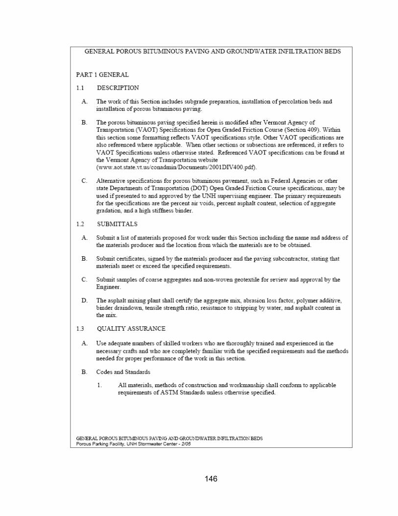
146

147

148

149

150

151
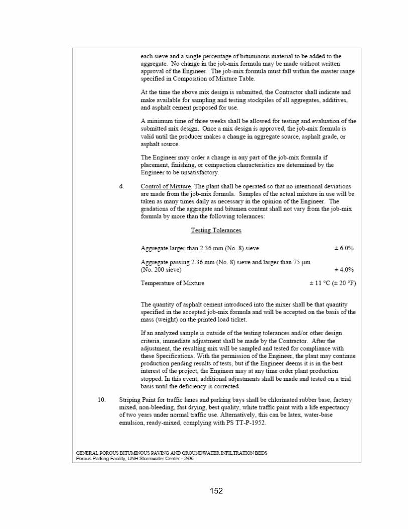
152

153

154

155

156

157
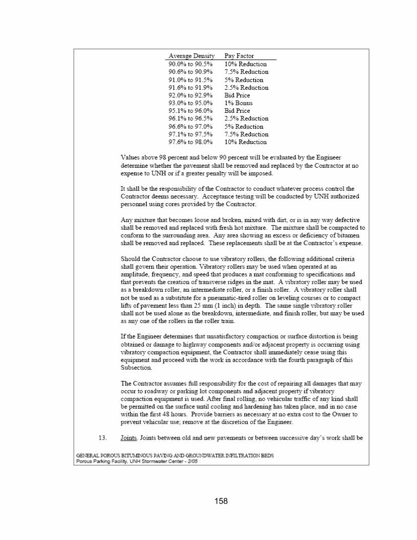
158

159

Figure 41. UNH PA specification package.
160
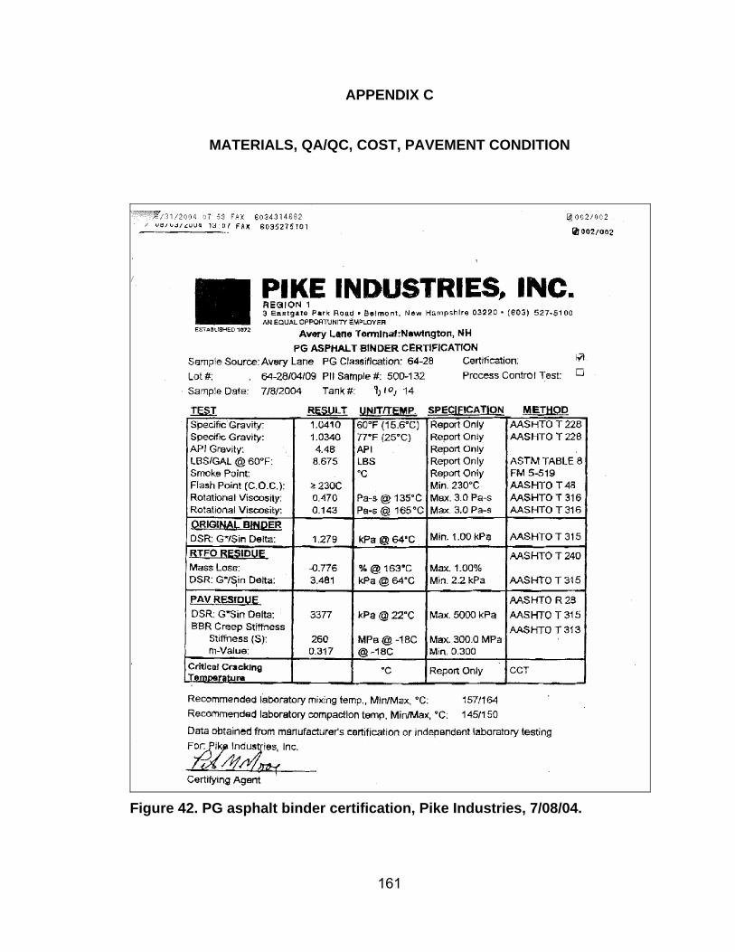
APPENDIX C
MATERIALS, QA/QC, COST, PAVEMENT CONDITION
Figure 42. PG asphalt binder certification, Pike Industries, 7/08/04.
161

Figure 43. Field notes from date of asphalt placement, Jo Daniel, 10/13/04.
Figure 44. Mix design report, Pike Industries, 10/07/04.
162

“Back pit” sample represents the bank run gravel used at the UNH PA lot.
“Back pit” sample represents the bank run gravel used at the UNH
Figure 45. Gradation of bank run gravel used as the filter course.
163

Figure 46. Paving quote, alternates by binder type, Pike Industries, 7/14/04.
164
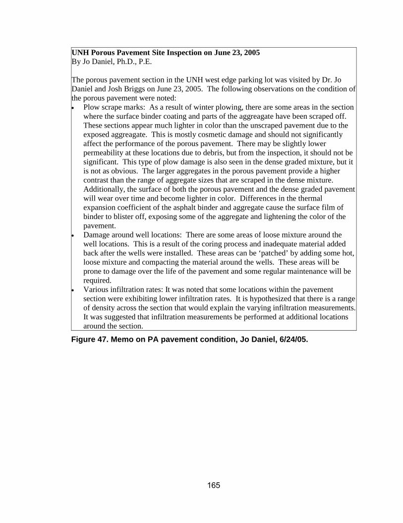
UNH Porous Pavement Site Inspection on June 23, 2005 By Jo Daniel, Ph.D., P.E. The porous pavement section in the UNH west edge parking lot was visited by Dr. Jo Daniel and Josh Briggs on June 23, 2005. The following observations on the condition of the porous pavement were noted: • Plow scrape marks: As a result of winter plowing, there are some areas in the section
where the surface binder coating and parts of the aggreagate have been scraped off. These sections appear much lighter in color than the unscraped pavement due to the exposed aggreagate. This is mostly cosmetic damage and should not significantly affect the performance of the porous pavement. There may be slightly lower permeability at these locations due to debris, but from the inspection, it should not be significant. This type of plow damage is also seen in the dense graded mixture, but it is not as obvious. The larger aggregates in the porous pavement provide a higher contrast than the range of aggregate sizes that are scraped in the dense mixture. Additionally, the surface of both the porous pavement and the dense graded pavement will wear over time and become lighter in color. Differences in the thermal expansion coefficient of the asphalt binder and aggregate cause the surface film of binder to blister off, exposing some of the aggregate and lightening the color of the pavement.
• Damage around well locations: There are some areas of loose mixture around the well locations. This is a result of the coring process and inadequate material added back after the wells were installed. These areas can be ‘patched’ by adding some hot, loose mixture and compacting the material around the wells. These areas will be prone to damage over the life of the pavement and some regular maintenance will be required.
• Various infiltration rates: It was noted that some locations within the pavement section were exhibiting lower infiltration rates. It is hypothesized that there is a range of density across the section that would explain the varying infiltration measurements. It was suggested that infiltration measurements be performed at additional locations around the section.
Figure 47. Memo on PA pavement condition, Jo Daniel, 6/24/05.
165

APPENDIX D
GROUNDWATER ELEVATION, WELLS, & SURFACE IC
Table 16. Surface IC via SIT, with raw and corrected values.
A B C A B C A B C11/18/04 16:30 1,414 1,114 438 5 5 25 1,343 1,058 328 PP 52 FH1/15/05 15:40 2,451 1,671 694 30 30 50 1,716 1,170 347 OCF 27 FH2/15/05 16:15 1,671 1,935 613 20 25 50 1,337 1,451 306 OCF 52 FH3/15/05 12:30 1,935 1,599 707 25 30 50 1,451 1,119 354 OCF 41 FH4/14/05 16:30 2,298 1,838 782 20 25 50 1,838 1,379 391 OCF 51 FH5/17/05 17:00 2,298 1,751 634 20 25 50 1,838 1,313 317 OCF 53 FH6/15/05 14:30 1,935 836 210 10 15 20 1,742 710 168 PP 42 FH7/17/05 14:30 1,532 668 334 5 10 40 1,455 602 201 PP 78 FH8/19/05 15:00 994 549 167 0 5 25 994 521 125 PP 73 CH9/30/05 14:30 1,081 668 210 15 20 50 919 535 105 OCF 61 CH11/4/05 15:00 1,050 320 153 20 35 75 840 208 38 OCF 51 CH1/12/06 15:00 1,838 1,050 230 25 35 75 1,379 683 57 CCPE 48 CH4/5/06 9:15 1,362 919 163 25 35 75 1,021 597 41 CCPE 36 CH5/31/06 10:30 1,935 566 NM 25 35 NM 1,451 368 CCPE 59 CH7/20/06 15:00 1,935 817 320 25 35 75 1,451 531 80 CCPE 73 CH8/26/06 10:30 1,414 694 NM 25 35 NM 1,061 451 CCPE 68 CH8/26/06 12:45 1,114 549 171 10 15 75 1,003 466 43 CCBR 70 CH10/2/06 14:00 1,414 566 230 10 15 75 1,273 481 57 CCBR 62 CH11/8/06 12:00 1,050 477 NM 10 15 NM 945 406 CCBR 54 CHPoint A data for 10/2/06 was collected on 10/16/06 due to obstruction of test location.PP - Plumbers putty, applied around the metal base in a ~1/2-inch diameter bead.OCF - Open cell foam insulation strip (for weather sealing doors and windows).CCPE - Closed cell polyethylene foam (for lifejacket flotation).CCBR - Closed cell black "rubber" foam, good seal at base if low head and warm.DRI - Double Ring Infiltration test. NM - Not Measured.Test Type: FH - Falling Head. CH - Constant Head.
Seal Type
Corr. Surf. IC (in/hr) Air T. (°F)
Test Type
% reduction in IC based on visual est. leakage (factors were seal type, air temp) and test type.
Est. % Red.Date Raw Surf. IC (in/hr)Time
166

Table 17. Groundwater elevations collected with manual sounder.
Well 1 Well 2 Well 3 Well 4 Well 5m Well 5d Well 6 Well 712/16/04 ND 90.33 92.00 NM NM 90.58 87.50 NM12/17/04 ND 90.45 92.10 NM NM 90.51 87.45 NM1/11/05 ND 89.84 91.95 NM NM 90.11 86.65 NM1/14/05 93.38 89.08 91.58 NM NM 90.51 86.47 NM1/14/05 92.37 NM 91.37 NM NM NM NM NM1/15/05 91.27 89.24 NM NM NM 90.60 86.59 NM1/18/05 89.96 88.74 91.36 NM NM 90.94 87.37 NM1/21/05 ND 90.16 92.36 NM NM 90.40 86.56 NM1/25/05 ND 89.63 91.76 NM NM 89.96 86.72 NM2/1/05 ND 88.89 90.60 NM NM 88.99 86.07 NM2/4/05 NM 88.58 90.32 NM NM 88.57 86.07 NM2/9/05 NM 88.62 90.11 NM NM 88.54 86.18 NM2/18/05 NM NM NM ND NM NM NM NM2/23/05 NM 90.60 92.51 ND NM 91.02 87.37 NM2/25/05 NM 90.40 92.53 ND NM 91.35 87.17 NM3/2/05 NM 90.15 91.92 ND NM 91.04 86.82 90.893/5/05 NM 89.58 NM NM 90.65 90.59 NM 90.98
3/8/2005 92.53 NM NM NM NM NM NM NM3/11/05 NM NM NM ND 91.01 91.09 NM 91.203/15/05 NM 89.65 91.78 ND 90.70 90.42 86.67 90.943/23/05 ND 91.05 91.67 91.26 91.67 91.46 87.37 91.604/2/05 92.58 NM NM 91.12 NM NM NM 91.144/6/05 90.18 92.49 96.04 91.17 91.20 91.08 90.24 90.99
4/21/05 89.55 91.24 93.51 90.95 91.26 91.11 87.72 90.526/2/05 89.77 91.86 94.63 91.36 91.22 91.08 88.37 91.056/29/05 93.37 90.07 91.80 90.26 91.10 91.02 86.32 91.138/16/05 ND 87.00 87.58 90.27 91.10 91.14 84.60 91.1210/5/05 ND ND ND 90.24 91.07 90.93 83.52 91.02
10/31/05 89.74 91.57 93.91 91.23 91.11 91.07 88.42 91.1411/30/05 89.82 92.44 93.86 91.17 91.15 91.21 88.59 91.002/23/06 ND 90.33 92.41 91.02 91.47 91.30 87.14 91.004/3/06 ND 89.39 91.09 ND 91.07 90.99 86.50 91.015/31/06 ND 91.10 93.32 90.92 91.14 91.02 87.54 90.97
10/16/06 ND 87.49 88.09 90.24 91.04 91.09 86.25 90.99
Date
NM - Not measured. ND - Not detected (plotted at bottom of screened interval).Well 5s was ND except for 3/02/05 (91.42 ft MSL) and 3/23/05 (91.58 ft MSL).
Groundwater Elevation (ft MSL)
167

Table 18. Construction data for groundwater monitoring wells.
Length (ft)
Slot No.
Depth Interval
Depth Class
Ground Surface
Top of Casing
Top of Screen
Bot. of Screen
Bot. of Bed
1 12/15/04 2" PVC 4.5 20 0'-4' shallow - 94.11 94.11 90.13 -2 12/15/04 2" PVC 5.0 20 5'-10' deep 96.07 95.90 91.30 86.30 -3 12/15/04 2" PVC 5.0 20 5'-10' deep 97.21 96.93 92.06 87.06 -4 2/18/06 1" SS 3.0 10 0'-4' shallow 95.56 95.16 93.49 90.49 91.45s 12/15/04 1" PVC 4.0 20 0'-4' shallow 95.49 95.40 95.40 91.42 91.25m 3/4/05 1" SS 3.0 10 4'-7' medium 95.49 95.32 91.65 88.65 91.25d 12/15/04 1" PVC 5.0 20 5'-10' deep 95.49 95.21 90.38 85.38 91.26 12/15/04 2" PVC 5.0 20 5'-10' deep 91.85 91.55 86.65 81.65 -7 2/28/05 1" SS 1.0 10 3'-4' medium 95.23 95.09 91.77 90.77 91.6
SDW-01 early '04 1" SS 5.0 10 0'-5' shallow 94.70 96.10 94.43 89.43 -SDW-02 early '04 1" SS 5.0 10 0'-5' shallow 91.12 93.22 91.55 86.55 -SDW-03 early '04 1" SS 5.0 10 0'-5' shallow 89.82 91.02 89.35 84.35 -Johnson Slot No. 20 corresponds to 0.0195 inch opening, Johnson Slot No. 10 to 0.0097 inch.Bottom of bed (porous media reservoir) elevations estimated at in-system wells from survey data.Wells SDW-01, SDW-02, and SDW-03 were destroyed during construction in Sept., 2004.Well 1 was angled at 27 degrees from vertical.
WellScreenDate
Installed
Dia. (in) and
Material
Elevation (ft MSL)
Figure 48. Groundwater monitoring well profile sketch. Hatched areas are either ground surface (top) or bottom of bed (lower). Elev. in ft MSL.
168

APPENDIX E
HYDROGRAPHS & HYDRAULIC PERFORMANCE
0
1
2
3
4
5
6
7
0 250 500 750 1,000 1,250 1,500
Time (min)
Flow
(gpm
)
0.00
0.01
0.02
0.03
0.04
0.05
5-M
in P
reci
p (in
)
D-Box FlowEffluent Flow
Precip
Figure 49. Hydrograph and hyetograph of the 5/07/05 event. Table 19. Hydraulic performance summary of the 5/07/05 event. Parameter Precip D-Box Effluentantecedent dry period (days) 4.1 - -start time (date/time) 5/7/05 3:00 - -end time (min) 965 995 3,660depth (in) 0.63 - -storm volume (gal) 2,199 2,648 2,199volume centroid (gal) 1,100 1,324 1,100time of centroid (min) 410 500 1,855lag time (min) - - 1,445kL - - 4.5peak intensity (in/5-min) 0.01 - -peak flow (gpm) 6.5 4.8 1.3time at peak flow (min) 595 605 1,560Kp - - 0.20
169

0
5
10
15
0 250 500 750 1,000 1,250Time (min)
Flow
(gpm
)
0
0.02
0.04
0.06
0.08
5-M
in P
reci
p (in
)
D-Box FlowEffluent FlowPrecip
Figure 50. Hydrograph and hyetograph of the 5/21/05 event. Table 20. Hydraulic performance summary of the 5/21/05 event. Parameter Precip D-Box Effluentantecedent dry period (days) 6.0 - -start time (date/time) 5/21/05 16:00 - -end time (min) 1,150 1,165 3,215depth (in) 0.91 - -storm volume (gal) 3,177 3,364 2,357volume centroid (gal) 1,588 1,682 1,179time of centroid (min) 460 485 1,780lag time (min) - - 1,320kL - - 3.9peak intensity (in/5-min) 0.02 - -peak flow (gpm) 13.0 9.7 1.96time at peak flow (min) 385 415 1,210Kp - - 0.15
170

0
20
40
60
80
0 200 400 600 800 1,000
Time (min)
Flow
(gpm
)
0
0.05
0.1
0.15
0.2
0.25
5-M
in P
reci
p (in
)
D-Box FlowEffluent FlowPrecip
Figure 51. Hydrograph and hyetograph of the 8/12/05 event. Table 21. Hydraulic performance summary of the 8/12/05 event. Parameter Precip D-Box Effluentantecedent dry period (days) 10.8 - -start time (date/time) 8/12/2005 18:00 - -end time (min) 765 860 3,595depth (in) 0.51 - -storm volume (gal) 1,780 1,884 108volume centroid (gal) 890 942 54time of centroid (min) 360 375 2,985lag time (min) - - 2,625kL - - 8.3peak intensity (in/5-min) 0.08 - -peak flow (gpm) 52.1 46.9 0.3time at peak flow (min) 365 370 2,945Kp - - 0.005
171

0
25
50
75
100
125
150
0 250 500 750Time (min)
Flow
(gpm
)
0
0.1
0.2
0.3
0.4
0.5
0.6
5-M
in P
reci
p (in
)
D-Box FlowEffluent FlowPrecip
Figure 52. Hydrograph and hyetograph of the 9/15/05 event. Table 22. Hydraulic performance summary of the 9/15/05 event. Parameter Precip D-Box Effluent
antecedent dry period (days) 10.7 - -start time (date/time) 9/15/2005 6:10 - -end time (min) 630 715 1,955depth (in) 0.89 - -storm volume (gal) 3,107 4,313 86volume centroid (gal) 1,553 2,157 43time of centroid (min) 545 560 1,500lag time (min) - - 955kL - - 2.8peak intensity (in/5-min) 0.18 - -peak flow (gpm) 117.3 83.3 0.2time at peak flow (min) 545 555 1,455Kp - - 0.002Effluent flow did not occur until 1,250 minutes, and was not discernible on this scale.
172

0
25
50
75
100
125
0 500 1,000 1,500 2,000Time (min)
Flow
(gpm
)
0
0.05
0.1
0.15
0.2
0.25
5-M
in P
reci
p (in
)
D-Box FlowEffluent Flow
Precip
Figure 53. Hydrograph and hyetograph of the 10/08/05 event. Table 23. Hydraulic performance summary of the 10/08/05 event. Parameter Precip D-Box Effluentantecedent dry period (days) 8.3 - -start time (date/time) 10/8/2005 0:05 - -end time (min) 1,865 2,075 10,145depth (in) 5.00 - -storm volume (gal) 17,453 23,273 17,453volume centroid (gal) 8,727 11,637 8,727time of centroid (min) 965 990 1,480lag time (min) - - 515kL - - 1.5peak intensity (in/5-min) 0.10 - -peak flow (gpm) 65.2 68.5 23.5time at peak flow (min) 745 750 800Kp - - 0.36
173

0
10
20
30
40
0 200 400 600 800 1,000Time (min)
Flow
(gpm
)
0
0.02
0.04
0.06
0.08
0.1
5-M
in P
reci
p (in
)
D-Box Flow
Effluent Flow
Precip
Figure 54. Hydrograph and hyetograph of the 11/30/05 event. Table 24. Hydraulic performance summary of the 11/30/05 event. Parameter Precip D-Box Effluentantecedent dry period (days) 5.6 - -start time (date/time) 11/30/2005 4:15 - -end time (min) 805 925 2,025depth (in) 0.69 - -storm volume (gal) 2,409 5,300 2,409volume centroid (gal) 1,204 2,650 1,204time of centroid (min) 535 545 1,100lag time (min) - - 56kL - - 2.
51
peak intensity (in/5-min) 0.03 - -peak flow (gpm) 19.5 24.1 2.8time at peak flow (min) 560 570 885Kp - - 0.14
174

0
10
20
30
40
0 200 400 600 800 1,000Time (min)
Flow
(gpm
)
0
0.05
0.1
0.15
0.2
5-M
in P
reci
p (in
)
D-Box Flow
Effluent Flow
Precip
Figure 55. Hydrograph and hyetograph of the 12/16/05 event. Table 25. Hydraulic performance summary of the 12/16/05 event. Parameter Precip D-Box Effluentantecedent dry period (days) 5.3 - -start time (date/time) 12/16/2005 4:40 - -end time (min) 625 1,120 2,270depth (in) 1.38 - -storm volume (gal) 4,817 5,390 1,586volume centroid (gal) 2,409 2,695 793time of centroid (min) 425 565 915lag time (min) - - 490kL - - 2.2peak intensity (in/5-min) 0.06 - -peak flow (gpm) 39.1 24.6 4.2time at peak flow (min) 425 555 770Kp - - 0.11
175

0
10
20
30
40
50
0 200 400 600 800 1,000Time (min)
Flow
(gpm
)
0
0.03
0.06
0.09
0.12
0.15
5-M
in P
reci
p (in
)
D-Box Flow
Effluent Flow
Precip
Figure 56. Hydrograph and hyetograph of the 1/11/06 event. Table 26. Hydraulic performance summary of the 1/11/06 event. Parameter Precip D-Box Effluentantecedent dry period (days) 6.2 - -start time (date/time) 1/11/2006 20:00 - -end time (min) 315 470 3,145depth (in) 0.59 - -storm volume (gal) 2,059 2,770 2,059volume centroid (gal) 1,030 1,385 1,030time of centroid (min) 185 190 1,700lag time (min) - - 1,515kL - - 9.2peak intensity (in/5-min) 0.05 - -peak flow (gpm) 32.6 27.6 1.8time at peak flow (min) 225 235 1,275Kp - - 0.06
176

0
5
10
15
20
25
0 500 1,000 1,500 2,000Time (min)
Flow
(gpm
)
0
0.03
0.06
0.09
0.12
5-M
in P
reci
p (in
)
D-Box Flow
Effluent Flow
Precip
Figure 57. Hydrograph and hyetograph of the 3/13/06 event.
Table 27. Hydraulic performance summary of the 3/13/06 event. Parameter Precip D-Box Effluentantecedent dry period (days) 15.3 - -start time (date/time) 3/13/2006 11:30 - -end time (min) 1,415 1,505 2,675depth (in) 0.92 - -storm volume (gal) 3,211 2,976 3,211volume centroid (gal) 1,606 1,488 1,606time of centroid (min) 660 700 1,855lag time (min) - - 1,195kL - - 2.7peak intensity (in/5-min) 0.04 - -peak flow (gpm) 26.1 14.8 4.2time at peak flow (min) 1,055 1,065 1,600Kp - - 0.16
177

0
10
20
30
40
50
0 500 1,000 1,500 2,000 2,500 3,000Time (min)
Flow
(gpm
)
0
0.03
0.06
0.09
0.12
0.15
5-M
in P
reci
p (in
)
D-Box Flow
Effluent Flow
Precip
Figure 58. Hydrograph and hyetograph of the 5/01/06 event. Table 28. Hydraulic performance summary of the 5/01/06 event. Parameter Precip D-Box Effluentantecedent dry period (days) 7.6 - -start time (date/time) 5/1/2006 22:40 - -end time (min) 2,130 7,755depth (in) 2.99 - -storm volume (gal) 10,437 11,307 5,581volume centroid (gal) 5,219 5,654 2,791time of centroid (min) 1,005 1,085 1,915lag time (min) - - 91kL - - 1.
09
peak intensity (in/5-min) 0.06 - -peak flow (gpm) 39.1 21.5 4.2time at peak flow (min) 1,900 1,005 1,605Kp - - 0.11
178

0
100
200
300
400
0 1,000 2,000 3,000Time (min)
Flow
(gpm
)
0
0.2
0.4
0.6
0.8
1
5-M
in P
reci
p (in
)
D-Box Flow
Effluent Flow
Precip
Figure 59. Hydrograph and hyetograph of the 6/01/06 event.
Table 29. Hydraulic performance summary of the 6/01/06 event. Parameter Precip D-Box Effluentantecedent dry period (days) 10.9 - -start time (date/time) 6/1/2006 17:45 - -end time (min) 1,035 1,160 3,370depth (in) 2.46 - -storm volume (gal) 8,587 NA 8,587volume centroid (gal) 4,294 NA 4,294time of centroid (min) 320 NA 1,100lag time (min) - - 78kL - - 3.
04
peak intensity (in/5-min) 0.41 - -peak flow (gpm) 267.2 206.8 14.0time at peak flow (min) 5 10 410Kp - - 0.05
179

APPENDIX F
MEETING MINUTES, UNH GROUNDS & ROADS, 10/12/06
180

181

182

Figure 60. Meeting minutes, UNH Grounds & Roads, 10/12/06.
183

APPENDIX G
REAL TIME WATER QUALITY STORM EVENT PLOTS
0
2000
4000
6000
D-Box Effluent
SC
(uS
/cm
)
6.5
7.5
8.5
9.5
10.5
11.5
D-Box Effluent
DO
(mg/
L)
5.5
6.0
6.5
7.0
7.5
8.0
D-Box Effluent
pH
40
45
50
55
60
65
D-Box Effluent
Tem
p (°
F)
Figure 61. Box plots of real time water quality for 4/20/05.
0
500
1000
1500
2000
2500
D-Box Effluent
SC
(uS
/cm
)
8
9
10
11
12
D-Box Effluent
DO
(mg/
L)
6.0
6.3
6.6
6.9
7.2
7.5
D-Box Effluent
pH
47
48
49
50
51
52
D-Box Effluent
Tem
p (°
F)
Figure 62. Box plots of real time water quality for 5/07/05.
0
500
1000
1500
2000
D-Box Effluent
SC
(uS
/cm
)
6.5
8.5
10.5
12.5
D-Box Effluent
DO
(mg/
L)
6.0
6.5
7.0
7.5
8.0
8.5
D-Box Effluent
pH
46
48
50
52
54
56
D-Box Effluent
Tem
p (°
F)
Figure 63. Box plots of real time water quality for 5/21/05.
184

0
500
1000
1500
D-Box Effluent
SC
(uS
/cm
)
5
6
7
8
D-Box Effluent
DO
(mg/
L)
3.5
4.5
5.5
6.5
7.5
D-Box Effluent
pH
63
68
73
78
83
88
D-Box Effluent
Tem
p (°
F)
Figure 64. Box plots of real time water quality for 8/12/05.
0
100
200
300
400
D-Box Effluent
SC
(uS
/cm
)
4.5
5.5
6.5
7.5
8.5
D-Box Effluent
DO
(mg/
L)
4.5
5.5
6.5
7.5
D-Box Effluent
pH62
66
70
74
D-Box Effluent
Tem
p (°
F)
Figure 65. Box plots of real time water quality for 9/15/05.
0
100
200
300
400
500
D-Box Effluent
SC
(uS
/cm
)
6
7
8
9
10
11
D-Box Effluent
DO
(mg/
L)
5
6
7
8
9
D-Box Effluent
pH
50
55
60
65
70
75
D-Box Effluent
Tem
p (°
F)
Figure 66. Box plots of real time water quality for 10/08/05.
185

0
500
1000
1500
2000
D-Box Effluent
SC
(uS
/cm
)
8
9
10
11
D-Box Effluent
DO
(mg/
L)
6.0
6.4
6.8
7.2
D-Box Effluent
pH
47
49
51
53
55
D-Box Effluent
Tem
p (°
F)
Figure 67. Box plots of real time water quality for 11/30/05.
0
2000
4000
6000
D-Box Effluent
SC
(uS
/cm
)
7
9
11
13
D-Box Effluent
DO
(mg/
L)
5.5
6.0
6.5
7.0
7.5
8.0
D-Box Effluent
pH30
35
40
45
50
55
D-Box Effluent
Tem
p (°
F)
Figure 68. Box plots of real time water quality for 12/16/05.
0
1000
2000
3000
4000
D-Box Effluent
SC
(uS
/cm
)
9
10
11
12
13
14
D-Box Effluent
DO
(mg/
L)
5.5
6.5
7.5
8.5
D-Box Effluent
pH
35
40
45
50
55
D-Box Effluent
Tem
p (°
F)
Figure 69. Box plots of real time water quality for 1/11/06.
186

Figure 72. Box plots of real time water quality for 6/01/06.
Figure 71. Box plots of real time water quality for 5/01/06.
Figure 70. Box plots of real time water quality for 3/13/06.
0
500
1000
1500
2000
D-Box Effluent
SC
(uS
/cm
)
5
6
7
8
9
10
D-Box Effluent
DO
(mg/
L)
4
5
6
7
8
D-Box Effluent
pH
50
60
70
80
D-Box Effluent
Tem
p (°
F)
0
500
1000
1500
2000
D-Box Effluent
SC
(uS
/cm
)
0
500
1000
1500
2000
2500
D-Box Effluent
SC
(uS
/cm
)
9
10
11
12
13
14
D-Box Effluent
DO
(mg/
L)
6.0
6.4
6.8
7.2
D-Box Effluent
pH
38
42
46
50
54
D-Box Effluent
Tem
p (°
F)
8
9
10
11
DO
(mg/
L)
D-Box Effluent5.5
6.0
6.5
7.0
7.5
8.0
D-Box
pH
187
Effluent46
49
52
55
D-Box Effluent
Tem
p (°
F)
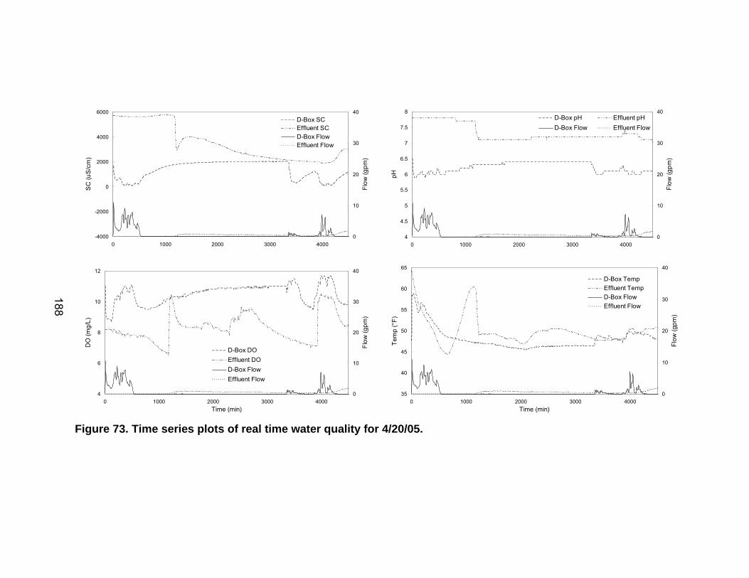
-4000
-2000
0
2000
4000
6000
0 1000 2000 3000 4000
SC
(uS
/cm
)
0
10
20
30
40
Flow
(gpm
)
D-Box SCEffluent SCD-Box FlowEffluent Flow
4
6
8
10
12
0 1000 2000 3000 4000Time (min)
DO
(mg/
L)
0
10
20
30
40
Flow
(gpm
)
D-Box DOEffluent DOD-Box FlowEffluent Flow
4
4.5
5
5.5
6
6.5
7
7.5
8
0 1000 2000 3000 4000
pH
0
10
20
30
40
Flow
(gpm
)
D-Box pH Effluent pHD-Box Flow Effluent Flow
35
40
45
50
55
60
65
0 1000 2000 3000 4000Time (min)
Tem
p (°
F)0
10
20
30
40
Flow
(gpm
)
D-Box TempEffluent TempD-Box FlowEffluent Flow
188
Figure 73. Time series plots of real time water quality for 4/20/05.

-1500
-1000
-500
0
500
1000
1500
2000
2500
0 1,000 2,000 3,000 4,000
SC
(uS
/cm
)
0
5
10
15
20
Flow
(gpm
)
D-Box SCEffluent SCD-BoxFlowEffluent Flow
6
7
8
9
10
11
12
0 1,000 2,000 3,000 4,000Time (min)
DO
(mg/
L)
0
5
10
15
20
Flow
(gpm
)
D-Box DO
Effluent DO
ID-Box Flow
Effluent Flow
5
5.5
6
6.5
7
7.5
0 1,000 2,000 3,000 4,000
pH
0
5
10
15
20
Flow
(gpm
)
D-Box pHEffluent pHD-Box FlowEffluent Flow
46
47
48
49
50
51
52
0 1,000 2,000 3,000 4,000Time (min)
Tem
p (°
F)0
5
10
15
20
Flow
(gpm
)
D-Box TempEffluent TempD-Box FlowEffluent Flow
189
Figure 74. Time series plots of real time water quality for 5/07/05.

-1000
0
1000
2000
0 1,000 2,000 3,000 4,000 5,000
SC
(uS
/cm
)
0
10
20
30
40
50
Flow
, gpm
D-Box SCEffluent SCD-Box FlowEffluent Flow
3
5
7
9
11
13
0 1,000 2,000 3,000 4,000 5,000Time, min
DO
(mg/
L)
0
10
20
30
40
50
Flow
, gpm
D-Box DOEffluent DOD-Box FlowEffluent Flow
4
5
6
7
8
9
0 1,000 2,000 3,000 4,000 5,000
pH
0
10
20
30
40
50
Flow
, gpm
D-Box pHEffluent pHD-Box FlowEffluent Flow
40
45
50
55
60
0 1,000 2,000 3,000 4,000 5,000Time, min
Tem
p (°
F)0
10
20
30
40
50
Flow
, gpm
D-Box TempEffluent TempD-Box FlowEffluent Flow
190
Figure 75. Time series plots of real time water quality for 5/21/05.

-1000
-500
0
500
1000
1500
0 500 1,000 1,500 2,000 2,500 3,000 3,500
SC
(uS
/cm
)
0
50
100
150
200
Flow
(gpm
)
D-Box SCEffluent SCD-Box FlowEffluent Flow
3.5
4
4.5
5
5.5
6
6.5
7
7.5
8
8.5
0 500 1,000 1,500 2,000 2,500 3,000 3,500Time (min)
DO
(mg/
L)
0
50
100
150
200
Flow
(gpm
)
D-Box DOEffluent DOD-Box FlowEffluent Flow
2
3
4
5
6
7
8
0 500 1,000 1,500 2,000 2,500 3,000 3,500
pH
0
50
100
150
200
Flow
(gpm
)
D-Box pHEffluent pHD-Box FlowEffluent Flow
50
60
70
80
90
0 500 1,000 1,500 2,000 2,500 3,000 3,500Time (min)
Tem
p (°
F)0
50
100
150
200
Flow
(gpm
)
D-Box TempEffluent TempD-Box FlowEffluent Flow
191
Figure 76. Time series plots of real time water quality for 8/12/05.

-300
-100
100
300
500
0 500 1,000 1,500 2,000
SC
(uS
/cm
)
0
100
200
300
Flow
(gpm
)
D-Box SCEffluent SCD-Box FlowEffluent Flow
3
3.5
4
4.5
5
5.5
6
6.5
7
7.5
8
0 500 1,000 1,500 2,000Time (min)
DO
(mg/
L)
0
100
200
300
Flow
(gpm
)
D-Box DOEffluent DOD-Box FlowEffluent Flow
3
4
5
6
7
8
0 500 1,000 1,500 2,000
pH
0
100
200
300
Flow
(gpm
)
D-Box pHEffluent pHD-Box FlowEffluent Flow
55
60
65
70
75
0 500 1,000 1,500 2,000Time (min)
Tem
p (°
C)
0
100
200
300
Flow
(gpm
)
D-Box TempEffluent TempD-Box FlowEffluent Flow
192
Figure 77. Time series plots of real time water quality for 9/15/05.
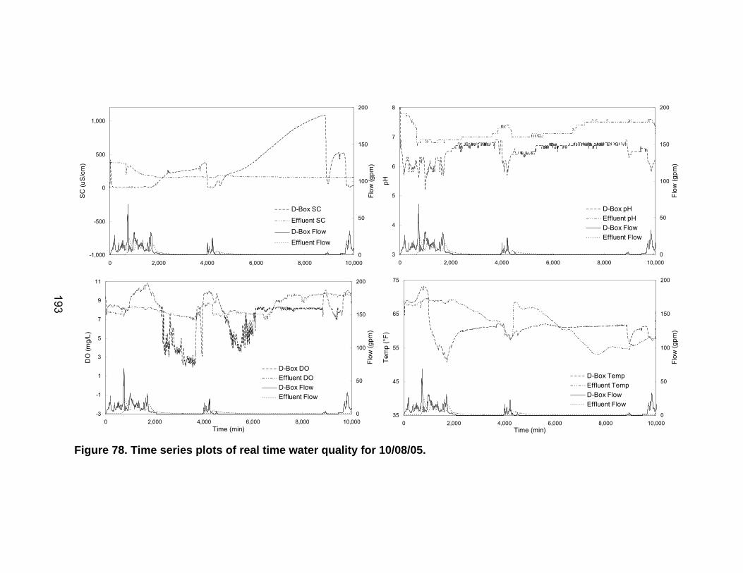
-1,000
-500
0
500
1,000
0 2,000 4,000 6,000 8,000 10,000
SC
(uS
/cm
)
0
50
100
150
200
Flow
(gpm
)
D-Box SC
Effluent SC
D-Box FlowEffluent Flow
-3
-1
1
3
5
7
9
11
0 2,000 4,000 6,000 8,000 10,000Time (min)
DO
(mg/
L)
0
50
100
150
200
Flow
(gpm
)D-Box DOEffluent DOD-Box FlowEffluent Flow
3
4
5
6
7
8
0 2,000 4,000 6,000 8,000 10,000
pH
0
50
100
150
200
Flow
(gpm
)
D-Box pHEffluent pHD-Box FlowEffluent Flow
35
45
55
65
75
0 2,000 4,000 6,000 8,000 10,000Time (min)
Tem
p (°
F)
0
50
100
150
200
Flow
(gpm
)
D-Box TempEffluent TempD-Box FlowEffluent Flow
193
Figure 78. Time series plots of real time water quality for 10/08/05.

-1000
-500
0
500
1000
1500
0 500 1,000 1,500 2,000 2,500
SC
(uS
/cm
)
0
25
50
75
100
Flow
(gpm
)
D-Box SCEffluent SCD-Box FlowEffluent Flow
6
7
8
9
10
11
0 500 1,000 1,500 2,000 2,500Time (min)
DO
(mg/
L)
0
25
50
75
100
Flow
(gpm
)
D-Box DOEffluent DOD-Box FlowEffluent Flow
5.5
6
6.5
7
0 500 1,000 1,500 2,000 2,500
pH
0
25
50
75
100
Flow
(gpm
)
D-Box pHEffluent pHD-Box FlowEffluent Flow
44
46
48
50
52
54
0 500 1,000 1,500 2,000 2,500Time (min)
Tem
p (°
F)0
25
50
75
100
Flow
(gpm
)
D-Box TempEffluent TempD-Box FlowEffluent Flow
194
Figure 79. Time series plots of real time water quality for 11/30/05.

-2000
0
2000
4000
6000
0 500 1,000 1,500
SC
(uS
/cm
)
0
30
60
90
120
150
Flow
(gpm
)
D-Box SCEffluent SCD-Box FlowEffluent Flow
4
6
8
10
12
0 500 1,000 1,500Time (min)
DO
(mg/
L)
0
30
60
90
120
150
Flow
(gpm
)
D-Box DOEffluent DOD-Box FlowEffluent Flow
5
6
7
8
0 500 1,000 1,500
pH
0
30
60
90
120
150
Flow
(gpm
)
D-Box pHEffluent pHD-Box FlowEffluent Flow
25
35
45
55
0 500 1,000 1,500Time (min)
Tem
p (°
F)0
30
60
90
120
150
Flow
(gpm
)
D-Box TempEffluent TempD-Box FlowEffluent Flow
195
Figure 80. Time series plots of real time water quality for 12/16/05.

-2000
0
2000
4000
0 500 1,000 1,500 2,000 2,500
SC
(uS
/cm
)
0
25
50
75
100
Flow
(gpm
)
D-Box SCEffluent SCD-Box FlowEffluent Flow
7
9
11
13
0 500 1,000 1,500 2,000 2,500Time (min)
DO
(mg/
L)
0
25
50
75
100
Flow
(gpm
)
D-Box DOEffluent DOD-Box FlowEffluent Flow
4
5
6
7
8
0 500 1,000 1,500 2,000 2,500
pH
0
25
50
75
100
Flow
(gpm
)
D-Box pHEffluent pHD-Box FlowEffluent Flow
20
30
40
50
0 500 1,000 1,500 2,000 2,500Time (min)
Tem
p (°
F)0
25
50
75
100
Flow
(gpm
)
D-Box TempEffluent TempD-Box FlowEffluent Flow
196
Figure 81. Time series plots of real time water quality for 1/11/05.

-500
500
1500
2500
0 500 1,000 1,500
SC
(uS
/cm
)
0
25
50
75
100
Flow
(gpm
)
D-Box SCEffluent SCD-Box FlowEffluent Flow
8
9
10
11
12
13
14
0 500 1,000 1,500Time (min)
DO
(mg/
L)
0
25
50
75
100
Flow
(gpm
)
D-Box DOEffluent DOD-Box FlowEffluent Flow
5.3
5.6
5.9
6.2
6.5
6.8
7.1
0 500 1,000 1,500
pH
0
25
50
75
100
Flow
(gpm
)
D-Box pHEffluent pHD-box FlowEffluent Flow
35
40
45
50
55
0 500 1,000 1,500Time (min)
Tem
p (°
F)0
25
50
75
100
Flow
(gpm
)
D-Box TempEffluent TempD-Box FlowEffluent Flow
197
Figure 82. Time series plots of real time water quality for 3/13/05.

-1000
-500
0
500
1000
1500
2000
0 2,500 5,000 7,500
SC
(uS
/cm
)
0
25
50
75
100
Flow
(gpm
)
D-Box SCEffluent SCD-Box FlowEffluent Flow
7
8
9
10
11
0 2,500 5,000 7,500
DO
(mg/
L)
0
25
50
75
100
Flow
(gpm
)D-Box DOEffluent DOD-Box FlowEffluent Flow
4
5
6
7
8
0 2,500 5,000 7,500
pH
0
25
50
75
100
Flow
(gpm
)
D-Box pHEffluent pHD-Box FlowEffluent Flow
45
50
55
0 2,500 5,000 7,500
Tem
p (°
F)
0
25
50
75
100
Flow
(gpm
)
D-Box TempEffluent TempD-Box FlowEffluent Flow
198
Figure 83. Time series plots of real time water quality for 5/01/05.

-1,000
-500
0
500
1,000
1,500
0 1,000 2,000 3,000
SC
(uS
/cm
)
0
200
400
600
800
Flow
(gpm
)
D-Box SCEffluent SCD-Box FlowEffluent Flow
2
4
6
8
10
0 1,000 2,000 3,000
DO
(mg/
L)
0
200
400
600
800
Flow
(gpm
)
D-Box DOEffluent DOD-Box FlowEffluent Flow
3
4
5
6
7
8
0 1,000 2,000 3,000
pH
0
200
400
600
800
Flow
(gpm
)
D-Box pHEffluent pHD-Box FlowEffluent Flow
40
50
60
70
80
0 1,000 2,000 3,000
Tem
p (°
F)
0
200
400
600
800
Flow
(gpm
)
D-Box TempEffluent TempD-Box FlowEffluent Flow
Figure 84. Time series plots of real time water quality for 6/01/05.
199

APPENDIX H
LIST OF DATA FILES ON ATTACHED CD-ROM
Files 1. Groundwater levels. 2. Storm event hydraulics and real time water quality. 3. Climate. 4. Storm event discrete sample water quality. 5. Water balance. 6. Chloride mass balance. 7. Pavement properties.
200