performance analysis of simulation-based multi-objective ... · pdf fileiii abstract...

Performance Analysis of Simulation-based Multi-objective

Optimization of Bridge Construction Processes Using High

Performance Computing

Shide Salimi

A Thesis

In the Department

Of

Building, Civil, and Environmental Engineering

Presented in Partial Fulfillment of the Requirements

For the Degree of Master of Applied Science (Building Engineering) at

Concordia University

Montreal, Quebec, Canada

November 2014

© Shide Salimi

CONCORDIA UNIVERSITY

School of Graduate Studies

This is to certify that the thesis prepared

By: Shide Salimi

Entitled: Performance Analysis of Simulation-based Multi-objective Optimization of

Bridge Construction Processes Using High Performance Computing

and submitted in partial fulfillment of the requirements for the degree of

Master of Applied Science (Building Engineering)

complies with the regulations of the University and meets the accepted standards with respect to

originality and quality.

Signed by the final Examining Committee:

Dr. T. Zayed Chair

Dr. Z. Zhu Examiner

Dr. A. Awasthi Examiner

Dr. A. Hammad Supervisor

Approved by

Chair of Department or Graduate Program Director

2014

Dean of Faculty

iii

ABSTRACT

Performance Analysis of Simulation-based Multi-objective Optimization of Bridge

Construction Processes Using High Performance Computing

Shide Salimi

Bridges constitute a crucial component of urban highways due to the complexity and

uncertain nature of their construction process. Simulation is an alternative method of analyzing

and planning the construction processes, especially the ones with repetitive and cyclic nature, and

it helps managers to make appropriate decisions. Furthermore, there is an inverse relationship

between the cost and time of a project and finding a proper trade-off between these two key

elements using optimization methods is important. Thus, the integration of simulation models with

optimization techniques leads to an advancement in the decision making process. In addition, the

large number of resources required in complex and large scale bridge construction projects results

in a very large search space. Therefore, there is a need for using parallel computing in order to

reduce the computational time of the simulation-based optimization. Most of the construction

simulation tools need an integration platform to be combined with optimization techniques. Also,

these simulation tools are not usually compatible with Linux environment which is used in most

of the massive parallel computing systems or clusters.

In this research, an integrated simulation-based optimization framework is proposed within one

platform to alleviate those limitations. A master-slave (or global) parallel Genetic Algorithm (GA)

is used as a parallel computing technique to decrease the computation time and to efficiently use

the full capacity of the computer. In addition, sensitivity analysis is applied to identify the

iv

promising configuration for GA and analyzing the impact of GA parameters on the overall

performance of the specific simulation-based optimization problem used in this research. Finally,

a case study is implemented and tested on a server machine as well as a cluster to explore the

feasibility of the proposed approach.

The results of this research showed better performance of the proposed framework in comparison

with other GA optimization techniques from the points of view of the quality of the optimum

solutions and the computation time. Also, acceptable improvements in the computation time were

achieved for both deterministic and probabilistic simulation models using master-salve parallel

paradigm (8.32 and 20.3 times speedups were achieved using 12 cores, respectively). Moreover,

performing the proposed framework on multiple nodes using a cluster system led to 31% saving

on the computation time on average. Furthermore, the GA was tuned using sensitivity analyses

which resulted in the best parameters (500 generations, population size of 200 and 0.7 as the

crossover probability).

v

ACNOWLEDGMENT

First and foremost, I wish to express my gratitude to my supervisor Professor Amin Hammad,

whose continuous intellectual and personal support, patience and encouragement made this degree

possible. His insightful guidance and suggestions were the most valuable help for me which

softened the difficulties of my research study.

I would like to a Dr. Dan Mazur, scientific computing analyst of the McGill University cluster, for

his generous and effective guidance and support during the last critical months of my research.

Also, I thank Mr. Pier-Luc St-Onge, another member of the McGill cluster technical support group,

for providing me with detailed information regarding the cluster environment.

Furthermore, I would like to use this opportunity to thank Mr. Mohammad Soltani for his

invaluable suggestions and help. I thank Mr. Mohammed Mawlana for providing me the basic

concepts of my study. All our discussions regarding different issues and topics related to my study

assisted me to improve my research and fully put the various pieces together.

My sincere thanks go to Ms. Sara Honarparst, who was always there for me with her positive

energy that gave me enough energy to walk towards my goals.

I feel grateful to my dear husband, Amir, for his immense support that helped me to complete my

research throughout the entire period of my study. I learned lots of important aspects of having a

good and respectable personality from him. I would like to give my special thanks to my beloved

parents, Shohre and Naser, for their endless love and spiritual support and encouragement in all

stages of my life. Also, I am grateful to all of my friends and collogues for so many good things

vi

they did for me to keep me energized and positive to complete my degree. I will be grateful forever

for your love.

vii

DEDICATION

To my beloved family, without whom none of my success would be possible.

viii

TABLE OF CONTENTS

TABLE OF CONTENTS .......................................................................................................... viii

LIST OF FIGURES .................................................................................................................... xii

LIST OF TABLES .................................................................................................................... xvii

LIST OF ABBREVIATIONS ................................................................................................... xix

CHAPTER 1 INTRODUCTION ........................................................................................... 1

1.1 Background ...................................................................................................................... 1

1.2 Problem Definition ........................................................................................................... 2

1.3 Research Objectives ......................................................................................................... 4

1.4 Thesis Organization.......................................................................................................... 4

CHAPTER 2 LITERATURE REVIEW ............................................................................... 6

2.1 Introduction ...................................................................................................................... 6

2.2 Bridge Construction Techniques ...................................................................................... 6

2.3 Accelerated Bridge Construction (ABC) ......................................................................... 7

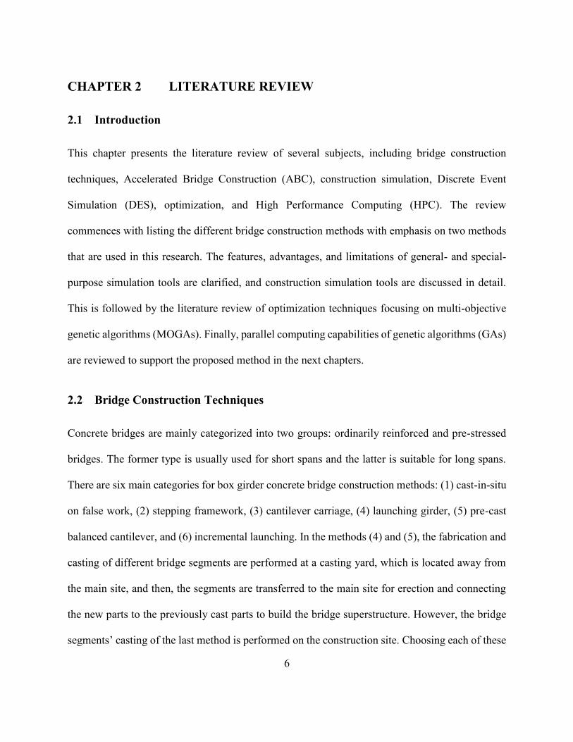
2.4 Selection of Construction Methods .................................................................................. 8

2.4.1 Precast Full-Span Concrete Box Girder Construction Method................................. 9

2.4.2 Precast Segmental Concrete Box Girder Construction ........................................... 11

2.5 Construction Simulation ................................................................................................. 21

2.5.1 Need for Construction Process Planning Tools ...................................................... 21

2.5.2 Simulation of Construction Processes .................................................................... 23

2.6 Construction Simulation Tools ...................................................................................... 24

2.6.1 Characteristics of Simulation Tools ........................................................................ 24

ix

2.6.2 General and Special-purposes Simulation Tools for Construction Applications ... 27

2.7 Discrete Event Simulation (DES) .................................................................................. 29

2.8 Optimization ................................................................................................................... 31

2.8.1 Genetic Algorithms for Multi-objective Optimization ........................................... 33

2.9 Simulation-based Optimization of Construction Processes ........................................... 39

2.9.1 Related Research ..................................................................................................... 41

2.10 High Performance Computing (HPC) ............................................................................ 45

2.10.1 Global Single-population Master-slave GAs .......................................................... 46

2.10.2 Multiple-deme Parallel GAs ................................................................................... 48

2.10.3 Single Population Fine-grained Parallel GAs ......................................................... 51

2.10.4 Hierarchical Parallel GAs ....................................................................................... 52

2.11 Parallel and Distributed Simulation ............................................................................... 54

2.11.1 Parallel Simulation of Construction Processes ....................................................... 55

2.11.2 Parallel Optimization of Construction Processes .................................................... 56

2.11.3 Parallel Simulation-based Optimization of Construction Processes ....................... 57

2.12 Summary and Conclusions ............................................................................................. 57

CHAPTER 3 RESEARCH METHODOLOGY ................................................................. 59

3.1 Introduction .................................................................................................................... 59

3.2 The Proposed Simulation-based Optimization Framework ........................................... 60

3.3 Using DES within SimEvents ........................................................................................ 64

3.3.1 Comparison of SimEvents and Stroboscope Simulation Tools .............................. 68

3.3.2 Stroboscope Simulation Model for Earthmoving Operation .................................. 69

3.3.3 SimEvents Model of Earthmoving Operation ......................................................... 70

x

3.3.4 Comparison of SimEvents and Stroboscope Simulation Models ........................... 72

3.4 Real-valued NSGA- ..................................................................................................... 75

3.5 Parallel Computing Approach ........................................................................................ 79

3.6 Simulation and Optimization Engines Interface ............................................................ 82

3.7 Sensitivity Analyses ....................................................................................................... 83

3.7.1 Effect of GA Parameters ......................................................................................... 83

3.7.2 Effect of Number of Cores ...................................................................................... 85

3.8 Comparison of Different Pareto Fronts .......................................................................... 85

3.9 Summary and Conclusions ............................................................................................. 87

CHAPTER 4 IMPLEMENTATION AND CASE STUDY ............................................... 89

4.1 Introduction .................................................................................................................... 89

4.2 Simulation Models Using SimEvents ............................................................................ 89

4.2.1 Precast Full Span Concrete Box Girder Construction Method ............................... 89

4.2.2 Validation of Full Span Simulation Model (Deterministic Mode) ......................... 91

4.2.3 Validation of Full Span Simulation Model (Probabilistic Mode) ........................... 91

4.2.4 Simulation of Precast Segmental Concrete Box Girder Construction Method using

SimEvents ............................................................................................................................. 95

4.3 Integration of MATLAB MOGA Optimization Tool and SimEvents Simulation Model

96

4.4 Validation of the Proposed Optimization Model using Full Span Construction Method

100

4.5 Sensitivity Analyses on the Server Machine ................................................................ 102

4.5.1 Effect of GA Parameters ....................................................................................... 104

4.6 Sensitivity Analyses on the Cluster .............................................................................. 113

xi

4.6.1 Effect of GA Parameters ....................................................................................... 113

4.7 Overall comparison of solutions obtained on server and cluster ................................. 120

4.8 Performance Comparison of the Server and Cluster .................................................... 125

4.9 Effect of Crossover Probability (𝑃𝑐) ............................................................................ 128

4.10 Effect of Number of Cores ........................................................................................... 129

4.11 Summary and Conclusions ........................................................................................... 136

CHAPTER 5 SUMMARY, CONCLUSIONS AND FUTURE WORK ......................... 139

5.1 Summary of research .................................................................................................... 139

5.2 Research contributions and conclusions ...................................................................... 140

5.3 Limitations and future work ......................................................................................... 141

REFERENCES ....................................................................................................................... 143

APPENDICES ....................................................................................................................... 158

Appendix A – MATLAB code of deterministic simulation (DES) ........................................ 159

Appendix B – MATLAB code of probabilistic simulation (DES) ......................................... 164

Appendix C – MATLAB code of multi-objective optimization (NSGA-) .......................... 169

Appendix D – MATLAB codes of different functions used in MOGA ................................. 170

Appendix E – MATLAB codes for calculating the Hypervolume indicator (Adapted from

(Kruisselbrink, 2011)) ............................................................................................................. 173

Appendix F – Profiling MATLAB codes ............................................................................... 174

Appendix G – Problem Faced Using SimEvents Simulation Tool and Parallel Computing .. 179

G.1 Memory leakage ........................................................................................................... 179

G.2 Speed Problem ............................................................................................................. 181

G.3 Problem with C-compiler: ............................................................................................ 183

xii

LIST OF FIGURES

Figure 2-1: Examples of precast full-span concrete box girder construction methods (VSL

International Ltd, 2013) ................................................................................................................ 11

Figure 2-2: Steps of full-span casting procedure (Continental Engineering Corporation, 2006) . 12

Figure 2-3: Precast full-span launching procedure steps (Continental Engineering Corporation,

2006) ............................................................................................................................................. 13

Figure 2-4: Long and short line casting methods (Casseforme, 2013; Shimizu Corporation, 2013)

....................................................................................................................................................... 14

Figure 2-5: Long line casting method (Abendeh, 2006) ............................................................... 15

Figure 2-6: Short line match-casting method (Maeda and Chun Wo Joint Venture, 1996) ......... 15

Figure 2-7: Span by span erection method using overhead gantry (Britt et al. 2014) .................. 17

Figure 2-8: Short line match-casting stripping process (Maeda and Chun Wo Joint Venture, 1996)

....................................................................................................................................................... 19

Figure 2-9: The moving process of the match-cast to the storage area and the fresh cast to the

position of the match-cast (Maeda and Chun Wo Joint Venture, 1996) ....................................... 20

Figure 2-10: Preparing to cast new segment (Maeda and Chun Wo Joint Venture, 1996) .......... 20

Figure 2-11: Production process of the new segment (Maeda and Chun Wo Joint Venture, 1996)

....................................................................................................................................................... 20

Figure 2-12: Different erection methods for segmental concrete box girder bridges (VSL


Figure 2-13: Examples of precast segmental concrete box girder construction methods (VSL


xiii

Figure 2-14: Master-slave parallel GA (Kandil & El-Rayes, 2006) ............................................. 47

Figure 2-15: Multiple-deme/population parallel GA (Cantú-Paz, 1997) ...................................... 49

Figure 2-16: Fine-grained parallel GAs paradigm (Sivanandam & Deepa, 2008) ....................... 53

Figure 3-1: Integration of DES and NSGA-ΙΙ............................................................................... 61

Figure 3-2: Simulink model of a wind turbine (MathWorks, 2014c) ........................................... 66

Figure 3-3: SimEvents components .............................................................................................. 67

Figure 3-4: Earth-moving operation model in Stroboscope (Adopted from Loannou & Martinez,

2006) ............................................................................................................................................. 70

Figure 3-5: Soil queue subsystem ................................................................................................. 71

Figure 3-6: Hauling activity and its duration distribution ............................................................ 71

Figure 3-7: Stopping criteria of the earth-moving operation model ............................................. 72

Figure 3-8: Complete simulation model of the earth-moving operation in SimEvent ................. 72

Figure 3-9: Chromosome structure of the real-valued GA ........................................................... 77

Figure 3-10: Global parallel computing paradigm ........................................................................ 81

Figure 3-11: McGill cluster (Guillimin) environment (McGill-HPC, 2014) ................................ 81

Figure 3-12: Schematic communication between multiple nodes ................................................ 83

Figure 3-13: Comparison of two intersecting Pareto fronts using Hypervolume Indicator (Adopted

from Zitzler et al., 2003) ............................................................................................................... 87

Figure 4-1: Simulation model of bridge construction using precast full-span launching method 92

Figure 4-2: Simulation Model of Bridge Construction Using Full Span Launching Method

(Mawlana & Hammad, 2013b) ..................................................................................................... 93

Figure 4-3: Simulation model of bridge construction using precast segmental launching method

....................................................................................................................................................... 97

xiv

Figure 4-4: Comparison of Pareto solutions obtained from NSGA- and fmGA (results of fmGA

are adapted from (Mawlana & Hammad, 2013b)) ...................................................................... 102

Figure 4-5: Non-Dominated Pareto solutions for different population sizes with 500 generations

..................................................................................................................................................... 105

Figure 4-6: Reference point for average Pareto solutions for different population sizes with 500

generations .................................................................................................................................. 106


..................................................................................................................................................... 108

Figure 4-8: Average Pareto solutions for different population sizes with 2000 generations...... 109

Figure 4-9: Average Pareto solutions for different population sizes with 4000 generations...... 109

Figure 4-10: Non-Dominated Pareto solutions for different number of generations with population

size of 50 ..................................................................................................................................... 110

Figure 4-11: Non-dominated Pareto solutions for different number of generations with population

size of 100 ................................................................................................................................... 111


size of 200 ................................................................................................................................... 112


size of 400 ................................................................................................................................... 113

Figure 4-16: Non-Dominated Pareto solutions with 500 generations ........................................ 115

Figure 4-14: Comparison of deterministic computation time for fixed number of generations

(Server) ....................................................................................................................................... 116

Figure 4-15: Comparison of deterministic computation time for fixed population sizes (Server)

..................................................................................................................................................... 116

xv


..................................................................................................................................................... 117


..................................................................................................................................................... 118


..................................................................................................................................................... 119

Figure 4-20: Non-Dominated Pareto solutions for different number of generations, with population

size of 50 ..................................................................................................................................... 120


size of 100 ................................................................................................................................... 122


size of 200 ................................................................................................................................... 123


size of 400 ................................................................................................................................... 124

Figure 4-24: Final performance comparison between the server and the cluster from quality of

solutions point of view ................................................................................................................ 126

Figure 4-25: Comparison of deterministic computation time for fixed population sizes (Cluster)

..................................................................................................................................................... 127


(Cluster) ...................................................................................................................................... 127

Figure 4-27: Time comparison between the performance of the Server machine and the cluster for

the fixed population sizes............................................................................................................ 131

xvi

Figure 4-28: Time comparison between the performance of the Server machine and the cluster for

the fixed number of generations ................................................................................................. 132

Figure 4-29: Set of optimum solutions for different values as crossover probability ................ 133

Figure 4-30: Saving in Computation time by increasing the number of cores in deterministic mode

(Server) ....................................................................................................................................... 134

Figure 4-31: Saving in computation time by increasing the number of cores (Server) .............. 135

Figure 4-32: Saving in computation time by increasing the number of nodes for 500 generations

and 200 population size in deterministic mode (Cluster) ........................................................... 136

xvii

LIST OF TABLES

Table 2-1: Usual properties of precast full-span concrete box girder bridges (NRS Bridge

Construction Equipment, 2008; Hewson, 2003) ........................................................................... 10

Table 3-1: Overtime Policy (Mawlana & Hammad, 2013b; RSMeans Engineering Department,

2011) ............................................................................................................................................. 63

Table 3-2: Building blocks used for modeling simulation models by Stroboscope and SimEvents

(Martinez, 1996; Lee et al., 2010)................................................................................................. 69

Table 3-3: Input entities of the simulation model with their corresponding values ..................... 70

Table 3-4: List of decision variables in multi-objective optimization problem (Mawlana &

Hammad, 2013b)........................................................................................................................... 78

Table 3-5: Arithmetic crossover operator for real-valued GAs .................................................... 79

Table 3-6: Specifications of cluster nodes (McGill-HPC, 2014) .................................................. 82

Table 4-1: Activities durations for deterministic simulation model ............................................. 93

Table 4-2: Comparison of the total duration and cost of the deterministic simulation models with

SimEvents and Stroboscope .......................................................................................................... 94

Table 4-3: Activities durations for stochastic simulation model (Mawlana & Hammad, 2013b) 95

Table 4-4: Comparison of the total duration and cost of the probabilistic simulation models with

SimEvents and Stroboscope .......................................................................................................... 98

Table 4-5: List of NSGA-ΙΙ Parameters (Phase I) ...................................................................... 103

Table 4-6: List of NSGA-ΙΙ Parameters (Phase II) ..................................................................... 103

Table 4-7: Hypervolume percentage of the Pareto fronts produced by the fixed number of

generations (Normalized values in the lower rows) ................................................................... 107

xviii

Table 4-8: Hypervolume percentage of the Pareto fronts produced by the fixed size of population

(Normalized values in the lower rows) ....................................................................................... 111

Table 4-9: Computation time (min) for deterministic mode on the server machine with 12 cores

..................................................................................................................................................... 114

Table 4-10: Hypervolume percentage of the Pareto fronts produced by fixed number of generations


Table 4-11: Hypervolume percentage of the Pareto fronts produced by fixed size of population


Table 4-12: Computation time (min) for deterministic runs on one node of the cluster with 12 cores

..................................................................................................................................................... 121

Table 4-13: Hypervolume percentage of the all Pareto fronts generated by server machine

considering one reference point (Normalized values in the lower rows) ................................... 123

Table 4-14: Hypervolume percentage of the all Pareto fronts generated by cluster considering one

reference point (Normalized values in the lower rows) .............................................................. 124

Table 4-15: Hypervolume percentage for fixed crossover probability (500 generations and

population size of 200)................................................................................................................ 128

Table 4-16: Improvement in the speed of running the integrated framework by the cluster while

fixing the population size ............................................................................................................ 130

Table 4-17: Parallel computation time for deterministic mode (Server) .................................... 134

Table 4-18: Parallel computation time for probabilistic mode (Server) ..................................... 134

Table 4-19: Parallel computation time using multiple nodes (Cluster) ...................................... 136

xix

LIST OF ABBREVIATIONS

Abbreviation Description

3D Three Dimensional

ABC Accelerated Bridge Construction

ACD Activity Cycle Diagram

AS Activity Scanning

ASPARAGOS Asynchronous Parallel Genetic Algorithm Optimization Strategy

BLX-α Blend Crossover

COOPS Construction Operation and Project Scheduling

CPM Critical Path Method

CPU Central Processing Unit

CSL Control and Simulation Language

CYCLONE CYCLic Operation Network

DES Discrete Event Simulation

DSS Decision-Support System

ES Event Scheduling

fmGA fast messy GA

GA Genetic Algorithm

GSP General Simulation Program

GSSS Genetic State-Space Search

HA Heuristic Algorithm

HGA Heuristic GA

HOCUS Hand Or Computer Universal Simulator

HPC High Performance Computing

LOB Line-Of-Balance

MOA Multi-objective Optimization Algorithm

MOEA Multi-Objective Evolutionary Algorithm

MOGA Multi-objective GA

MOPSO Multi-Objective Particle Swarm Optimization

MPP Massive Parallel Processor

ND Normal Distribution

NSGA Non-dominated Sorting Genetic Algorithm

PCX Parent Centric Crossover

PDL Process Description Language

PI Process Interaction

PMX Partially Matched Crossover

PPX Precedence Preservative Crossover

PT Post Tensioned

RBM Resource-Based Modeling

RESQUE RESource based QUEuing

SBX Simulated Binary Crossover

SPX Simplex Crossover

UD Uniform Distribution

xx

UNDX Unimodal Normal Distribution Crossover

1

CHAPTER 1 INTRODUCTION

1.1 Background

Highway infrastructures in North America are relatively old structures; therefore, there is a great

necessity of reconstruction work on existing highways. These construction or renovation activities

have great impact on traffic flow, workforces, business and other community functions (Li et al.,

2010; Shan et al., 2007; Yifu, 2005; Yuan & Ren, 1999). Due to different factors, such as change

orders during the construction work because of detecting conflicts between project components,

economic and social activities, the costly equipment and materials needed for construction

processes, highway projects usually overrun in budget and time (Wu et al., 2005; Serag et al.,

2010; Vidalis & Najafi, 2002). Furthermore, traffic disruption during the construction operations

results in dangerous work space for workers as well as drivers and passengers (Holt, 2008).

Roads, tunnels, and bridges form the urban highways, in which bridges part is a crucial one due to

the complexity and uncertain nature of their construction process. The main factors causing

uncertainties associated with bridge construction operations are the lack of knowledge and

experience about different construction methods, and the spatial-temporal environment that may

have potential conflicts (Zhang & Hammad, 2005).

On the other hand, construction processes become so complex and difficult to analyze and optimize

recently (Martinez, 1996). Simulation is an alternative method of analyzing and planning the

construction processes especially the ones with repetitive and cyclic nature (AbouRizk & Halpin,

1990). Therefore, simulation of construction processes plays an important role in the modern world

and helps managers to have better understanding of the condition and different levels of the

2

construction processes to make appropriate decisions when it is needed (AbouRizk & Hajjar,

1998). Simulation is a procedure of imitating the behavior of some situations or a real-world

processes over time by means of using simpler models. Simulation in construction can be used for

different purposes such as productivity measurement, planning and resource allocation, risk

analysis, site planning, and comparing the results of various construction methods (AbouRizk et

al., 1992; Thomas, et al., 1990; Eshtehardian et al., 2008). Simulation of earthmoving operations

(Halpin & Riggs, 1992; Marzouk & Moselhi, 2003), structural steel erection process (Al-Sudairi

et al., 1999) and simulation of balanced cantilever bridges (Marzouk et al., 2008) are some

examples of using simulation for construction processes. Some researchers used simulation

particularly to investigate the performance of bridge construction methods. For example, Huang

et al. (1994) simulated the construction of the deck of a cable-stayed bridge using balanced

cantilever method, Marzouk et al. (2006) studied the simulation of the construction of concrete

box girder bridge deck using cast-in place on false-work and stepping formwork, they continued

their research by working on incremental launching method in 2007, and then, simulation of bridge

deck construction using cast-in place on false-work and cantilever carriage methods in 2009

(Marzouk et al., 2007; Said et al., 2009). Works done by Huang et al. (1994) and Mawlana et al.

(2012) are other examples in this area with focus on cable-stayed bridges and the construction of

precast concrete box girder using the full-span launching gantry method, respectively.

1.2 Problem Definition

Due to the large number of factors affecting the construction and rehabilitation processes of

bridges, these processes are highly complex for decision makers especially in terms of minimizing

the time and cost of the projects. They have to find the optimum strategy to complete the projects

3

successfully on time and within the budget considering all other constraints. Generally, there is an

inverse relationship between the cost and time of a project; since, whenever the duration of a

project is shortened, the cost of the project (i.e. the direct cost of labor, equipment, material etc.)

will increase considerably. Hence, finding a proper trade-off between these two key elements using

optimization methods has become a crucial issue for project managers (Feng et al., 2000).

On the other hand, as stated earlier, simulation models are more and more needed in order to model

the uncertainties associated with these projects (Yang et al., 2012). Therefore, the integration of

simulation models with optimization techniques leads to an advancement in the decision making

process.

In addition, due to the large number of resources required in complex and large scale construction

projects, such as bridge construction processes which results in a very large search space, there is

a need for High Performance Computing (HPC) in order to reduce the computational time. There

are several special purpose tools to implement the simulation of construction processes with

different advantages, limitations, and capabilities. Although simulating construction processes

using these tools is very easy to learn and to use, the combination of these tools with optimization

techniques is difficult and an integration platform is needed. On the other hand, these simulation

tools are not usually compatible with Linux environment which is used in most of the massive

parallel computing systems or clusters. Therefore, the lack of easy interaction of simulation and

optimization engines in the same integrated environment, which also supports their execution on

the operating system of the clusters, is the main motivation of this research.

4

Finally, the values of the optimization parameters affect directly the performance of the

optimization algorithm. Therefore, finding the promising configuration for optimization method

and analyzing the impact of these parameter on the overall performance of a system is another

challenge that researchers are facing when working with optimization algorithms.

1.3 Research Objectives

Given the above problems, the main objectives of this research are defined as follows:

1. Simulating different construction methods of precast box girder bridge construction

projects using a new simulation tool that can be used in a HPC environment.

2. Investigating High Performance Computing of the integration of the simulation model with

multi-objective optimization algorithm in a single platform in order to improve the

performance of the proposed framework in HPC environment.

3. Reducing the computational effort by performing sensitivity analysis to tune the

optimization algorithm and to find the best number of cores used in parallel.

1.4 Thesis Organization

This thesis is organized as follows:

Chapter 2 Literature Review: In this chapter the different bridge construction methods are

discussed with emphasis on two methods that are used in this research. The features, advantages,

and limitations of general- and special-purpose simulation tools are clarified, and construction

simulation tools are discussed in detail. Also, optimization techniques focusing on multi-objective

5

genetic algorithms (MOGAs) and parallel computing capabilities of genetic algorithms (GAs) are

reviewed.

Chapter 3 Research Methodology: This chapter will explain the research methodology employed

to develop a simulation-based multi-objective optimization model that can be used in HPC

environment for the planning and scheduling of precast concrete box girder bridge construction

projects.

Chapter 4 Research Implementation and Case Study: The implementation and applicability of the

proposed simulation-based optimization framework using HPC is investigated in this chapter.

Then, the feasibility of the developed models will be demonstrated by considering a case study.

This is followed by applying the HPC to investigate the time saving achieved in comparison with

a regular PC computation platform. Then, sensitivity analyses of the GA parameters as well as the

number of cores and nodes used to run the proposed framework are performed.

Chapter 5 Summary, Conclusions, and Future Work: In this chapter, a summary of this research

study is presented and its contributions are highlighted. Moreover, the limitations of the current

work are investigated and finally the recommendations for the future research are suggested.

6

CHAPTER 2 LITERATURE REVIEW

2.1 Introduction

This chapter presents the literature review of several subjects, including bridge construction

techniques, Accelerated Bridge Construction (ABC), construction simulation, Discrete Event

Simulation (DES), optimization, and High Performance Computing (HPC). The review

commences with listing the different bridge construction methods with emphasis on two methods

that are used in this research. The features, advantages, and limitations of general- and special-

purpose simulation tools are clarified, and construction simulation tools are discussed in detail.

This is followed by the literature review of optimization techniques focusing on multi-objective

genetic algorithms (MOGAs). Finally, parallel computing capabilities of genetic algorithms (GAs)

are reviewed to support the proposed method in the next chapters.

2.2 Bridge Construction Techniques

Concrete bridges are mainly categorized into two groups: ordinarily reinforced and pre-stressed

bridges. The former type is usually used for short spans and the latter is suitable for long spans.

There are six main categories for box girder concrete bridge construction methods: (1) cast-in-situ

on false work, (2) stepping framework, (3) cantilever carriage, (4) launching girder, (5) pre-cast

balanced cantilever, and (6) incremental launching. In the methods (4) and (5), the fabrication and

casting of different bridge segments are performed at a casting yard, which is located away from

the main site, and then, the segments are transferred to the main site for erection and connecting

the new parts to the previously cast parts to build the bridge superstructure. However, the bridge

segments’ casting of the last method is performed on the construction site. Choosing each of these

7

construction methods depends on the experience of the designers and contractors, availability of

resources, and technical restrictions. The incremental launching method has the benefits of less

need for temporary false-work and other equipment required for cast-in-situ techniques (Marzouk

et al. 2007).

2.3 Accelerated Bridge Construction (ABC)

Transportation plays an important role in the development of overall economy. Highway networks

as one main part of the society infrastructure need innovative technologies to enhance their

performance when they have been aging and reaching to their design life. Due to increasing traffic

passing the highway networks, conventional construction methods are not anymore viable

solutions to perform reconstruction works on these systems (Tang, 2014).

Use of innovating planning, design, materials, and bridge construction methods to decrease the

construction, replacing, and rehabilitating impacts on society is defined as ABC (Accelerated

Bridge Construction, 2014). To reduce dependency on time consuming on-site activities and

weather conditions tied to conventional construction techniques, the Federal Highway

Administration pushes ABC as a proper replacement of conventional construction methods

(Nielsen, 2013). These two approaches can be compared from different aspects. As it is obvious

from its name, ABC is much faster than conventional construction methods. On the other hand,

considering the trade-off between the cost and time leads to cheaper processes for conventional

methods. These costs include operational and maintenance costs of the bridges. For example,

bridges constructed based on the ABC technique need more overlays through the years due to the

amount of their deck joints which results in more maintenance costs for these types of bridges.

8

From safety point of view, ABC projects always are safer in comparison with conventional

methods due to their shorter construction period which protects workforce from long periods of

working on dangerous work sites which have traffic flow (Nielsen, 2013). Therefore, the main

advantages of the ABC over conventional construction methods are building bridges faster and

with minimum traffic disruption by shifting most construction activities into a precast yard or

factory, better quality control of the bridge’s elements, higher safety during construction, and less

environmental impacts. These advantages can be achieved by using innovative planning, design,

materials and construction methods (Federal Highway Administration, 2013; Fowler, 2006).

One of commonly used ABC methods is the use of precast concrete bridges which can be utilized

for most bridge projects (WisDOT Bridge Manual, 2013). In this method, precast spans of the

bridges can be erected by cranes standing on land or mounted on a barge, or by using cranes and

gantries on the bridge structure (Gerwick, 1993). In this research, the focus is on the construction

of concrete box girder bridges using the following construction methods: (1) precast full-span

erection using launching gantry; and (2) precast segmental span erection using launching gantry.

2.4 Selection of Construction Methods

The selection of construction methods for construction projects has a high effect on the project

productivity, quality and cost. Ferrada et al. (2013) proposed a knowledge management approach

incorporating both knowledge management techniques and technologies to enhance the decision-

making process of construction methods. They generated a knowledge-based portal called

Construction Methods Knowledge System (SCMC) to enable easy access and provide a decision-

making support system. The proposed system focuses mainly on the most influential decision

9

criteria for selecting construction methods include project duration, cost, product characteristics,

construction method characteristics, and environmental characteristics. Based on interviews with

some experts on construction methods selection, the performance of the system was validated from

different aspects. Most of the respondents believed that the system works well and helps to make

more informed decisions by gathering all the information needed in one place. In addition, they

highlighted that using the system leads to the increase of the productivity by time saving achieved

from easy access to information and search for alternative methods of construction. This system,

also, reduces the dependency on individual knowledge by storing all the information and

knowledge gained in organizational databases (Ferrada et al., 2013).

2.4.1 Precast Full-Span Concrete Box Girder Construction Method

This construction method is useful for elevated bridges placed in congested areas with many

obstacles, and which have spans with similar length. The advantages of this construction method

are: (1) minimizing traffic disruption (Mawlana, 2013); (2) improving construction quality due to

quality control at the precast yard (Erdogan, 2009); (3) decreasing in the construction cost and

time (Pan et al., 2008); (4) enhance the production rate (Mawlana, 2013); and (5) better safety due

to less need for onsite activities (VSL International Ltd, 2013). On the other hand, the dependency

on high level of technology, high equipment cost, being inapplicable for areas with difficult access,

and the need for vast areas for casting and storing are disadvantages of this method (Hewson,

2003). Figure 2-1 shows some examples of applying this construction method. Table 2-1 illustrates

the properties of bridges constructed based on the precast full-span concrete box girder

construction method.

10

Table 2-1: Usual properties of precast full-span concrete box girder bridges (NRS Bridge

Construction Equipment, 2008; Hewson, 2003)

Properties Span Length Span Weight Span Width

Value of the Properties 30-55 m 600-1500 tons 5- more than 12 m

There are two main stages in applying precast full-span concrete box girder bridge construction

method, including fabrication of full-spans of concrete box girder at the pre-casting yard, and

transporting prefabricated spans to the main site and erecting them using various techniques onsite.

At first, the reinforcement and stressing ducts of the bottom slab and the webs of the span are

erected, and then, the inner mold is installed followed by placing the reinforcement and stressing

ducts of the top slab. After finishing reinforcement work, the rebar cage is put into an outer mold

to do the casting. When the concrete cured and reached an acceptable strength, the inner mold is

removed. Next, the first pre-stressing procedure is performed to make the full-span ready for

transportation to the storage area where the full-span is completely cured and stored. After

completing concrete curing, the second stage of pre-stressing process is done (Continental

Engineering Corporation, 2006). Figure 2-2 illustrates the whole process of preparing precast full-

span concrete box girder.

In second stage of this construction method, the precast full-span is transported to the main site by

means of trailers for erection. Then, the girder is delivered along completed deck of bridge by

trolley to its launching location. After that, the full-span is lift from trolley by means of gantry's

lifting frames. The girder is moved forward to reach to its right position between two piers to be

placed. In next step, the launcher repositions to lift next full-span (Continental Engineering

Corporation, 2006; VSL International Ltd, 2013).

11

(a) Taiwan High speed Rail (2000-2004)

(b) No. 2 Road Bridge – British Colombia (1993)

Figure 2-1: Examples of precast full-span concrete box girder construction methods (VSL

International Ltd, 2013)

2.4.2 Precast Segmental Concrete Box Girder Construction

Precast segmental concrete box girder construction method is based on casting short segments with

high quality concrete which are in sizes that can be transported to the main construction site, and

then erected to be connected to each other to form the full-span.

In other words, the deck of the bridge is comprised of these small segments incrementally

constructed on each pier. The segments are firstly reinforced with mild steel, and then connected

by post-tensioning after erection (Lacey & Breen, 1969). This method results in fast delivery of

the project by having the capability of building girders and piers simultaneously. Also, using this

construction method without scaffolding in situ has less disruption to the traffic flow which makes

this method very useful for crowded areas. Segmental method improves the construction quality

due to factory production of segments which contains quality control on the segments by skilled

workers (Continental Engineering Corporation, 2006; Erdogan, 2009).

12

(a) Erection of reinforcement and stressing ducts

of the bottom slab and the webs (b) Inner mold installation and placing the

reinforcement and stressing ducts of the top slab (c) Putting rebar cage into outer mold

(d) Pouring concrete (e) Curing concrete (f) Removing inner mold

(g) First stage of pre-stressing (h) Transporting completed span to the

storage area (i) Second stage of pre-stressing

Figure 2-2: Steps of full-span casting procedure (Continental Engineering Corporation, 2006)

13

(a) Transporting precast full-span to the main site

(b) Delivering the girder to the launcher by trolley

(c) Lifting the girder by lifting frame (d) Moving the girder forward

(e) Locating the span in its right position (f) Reposition launcher to the next span

Figure 2-3: Precast full-span launching procedure steps (Continental Engineering Corporation,

2006)

Like precast full-span box girder bridge construction method, this technique has two main stages.

Firstly, concrete box girder segments should be casted at the casting yard, and then, they are

transported to the main site for erection and building the full-spans. Match-casting technique is the

most popular casting method in construction of the precast segmental concrete box girder bridges.

14

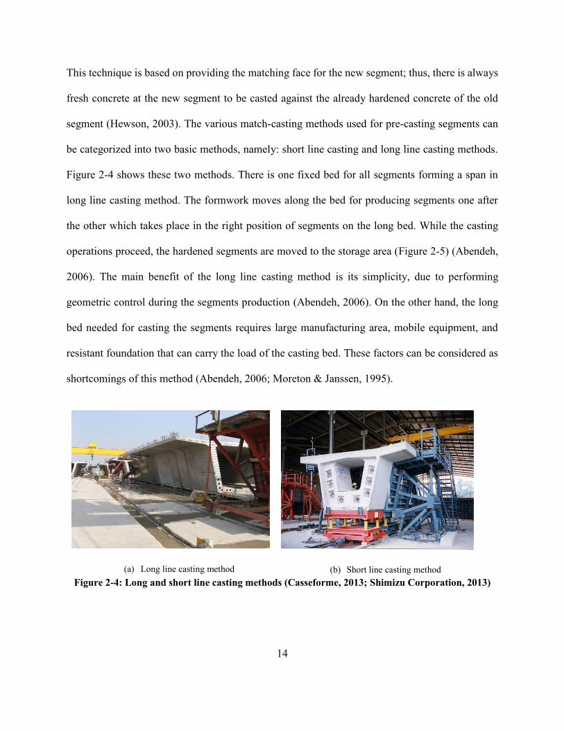
This technique is based on providing the matching face for the new segment; thus, there is always

fresh concrete at the new segment to be casted against the already hardened concrete of the old

segment (Hewson, 2003). The various match-casting methods used for pre-casting segments can

be categorized into two basic methods, namely: short line casting and long line casting methods.

Figure 2-4 shows these two methods. There is one fixed bed for all segments forming a span in

long line casting method. The formwork moves along the bed for producing segments one after

the other which takes place in the right position of segments on the long bed. While the casting

operations proceed, the hardened segments are moved to the storage area (Figure 2-5) (Abendeh,

2006). The main benefit of the long line casting method is its simplicity, due to performing

geometric control during the segments production (Abendeh, 2006). On the other hand, the long

bed needed for casting the segments requires large manufacturing area, mobile equipment, and

resistant foundation that can carry the load of the casting bed. These factors can be considered as

shortcomings of this method (Abendeh, 2006; Moreton & Janssen, 1995).

(a) Long line casting method

(b) Short line casting method

Figure 2-4: Long and short line casting methods (Casseforme, 2013; Shimizu Corporation, 2013)

15

Figure 2-5: Long line casting method (Abendeh, 2006)

Most match-cast segmental bridges use the short line method since it can be used for any shape of

deck alignment (Benaim, 2008). In short line casting method, segments are casted by using fixed

forms next to the previously cast segment to have complete fitting match-cast joint (Moreton &

Janssen, 1995; Rotolone, 2008). This method needs smaller space in comparison with long line

technique, and is more proper for horizontal and vertical curves as the long line method requires

changes in soffit configuration from one span of the bridge to another (Abendeh, 2006; Moreton

& Janssen, 1995). Precise adjustment of the match-cast segments is the major disadvantage of the

short line match-casting technique (Abendeh, 2006). Figure 2-6 shows the front and side views of

the short line match-casting method.

Figure 2-6: Short line match-casting method (Maeda and Chun Wo Joint Venture, 1996)

When the fresh segment is cured properly, its strength is controlled and the stripping process starts

including removal of (a) the inflatable inner tubes from fresh cast connected to the match-cast, and

16

(b) all the top slab inserts, such as scaffold tubes, top temporary post-tensioned (PT) holes and

temporary access (Figure 2-8(a) and (b)) (Maeda and Chun Wo Joint Venture, 1996). In the next

Step, the internal formwork is removed (Figure 2-8(c)); then, the supporting rods on two sides and

the external formwork is lowered down (Figure 2-8(d)).

(a) Transport the match-cast to the storage area

To transport the match-cast to the temporary storage area, the bulk head is retracted, and then the

fresh cast with the bottom formwork is moved to the position of the match-cast by means of the

cart. Figure 2-9 demonstrates this process.

(b) Preparing to cast new segment

In this step, new bottom formwork is placed, and the bulk head is moved inward again to be

prepared for casting a new segment. After cleaning the whole set of formwork, the external

formwork and supporting rods are raised to their position (Figure 2-10).

(c) Production process of the new segment

In order to produce the new segment, a steel cage, which is prepared in advance, is firstly placed

inside the formwork; then, inflatable inner tubes and all the top slab inserts are installed. After that,

the internal formwork is moved to its position within the external formwork. Finally, a new

segment is produced after pouring and curing of concrete, and the whole process will be repeated

(Figure 2-11) (Maeda and Chun Wo Joint Venture, 1996).

In the second stage of precast segmental construction method, the precast segmental concrete box

girders are transferred to the construction site by means of a trailer to be erected and form the full

bridge spans. There are several erection methods for segmental box girder bridges, such as span-

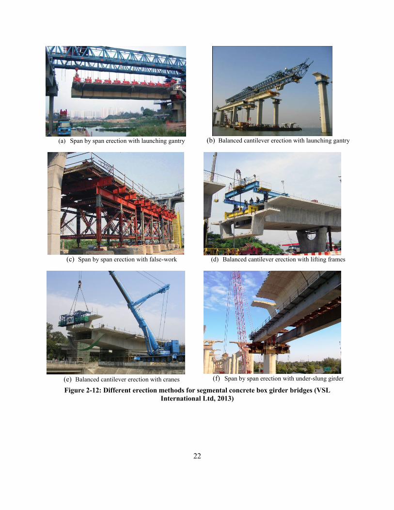
by-span erection, balanced cantilever construction, progressive erection of precast segmental

decks, and incremental launching (Benaim, 2008). The span by span erection method which is

17

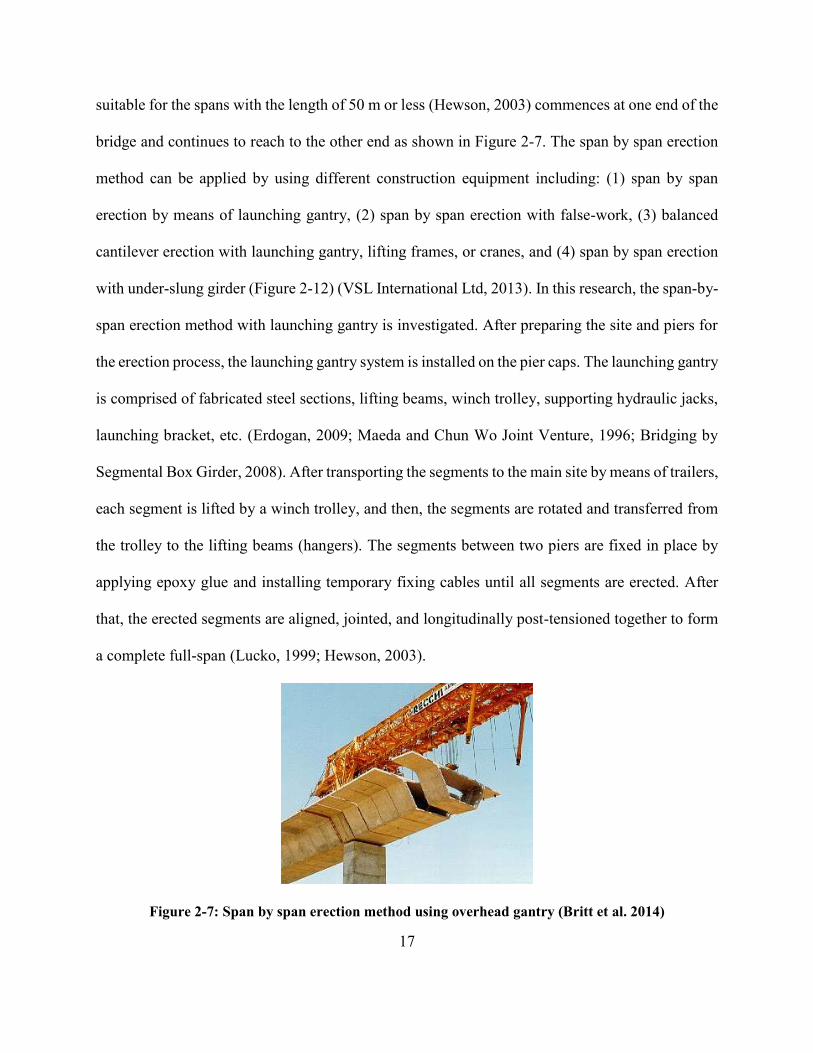
suitable for the spans with the length of 50 m or less (Hewson, 2003) commences at one end of the

bridge and continues to reach to the other end as shown in Figure 2-7. The span by span erection

method can be applied by using different construction equipment including: (1) span by span

erection by means of launching gantry, (2) span by span erection with false-work, (3) balanced

cantilever erection with launching gantry, lifting frames, or cranes, and (4) span by span erection

with under-slung girder (Figure 2-12) (VSL International Ltd, 2013). In this research, the span-by-

span erection method with launching gantry is investigated. After preparing the site and piers for

the erection process, the launching gantry system is installed on the pier caps. The launching gantry

is comprised of fabricated steel sections, lifting beams, winch trolley, supporting hydraulic jacks,

launching bracket, etc. (Erdogan, 2009; Maeda and Chun Wo Joint Venture, 1996; Bridging by

Segmental Box Girder, 2008). After transporting the segments to the main site by means of trailers,

each segment is lifted by a winch trolley, and then, the segments are rotated and transferred from

the trolley to the lifting beams (hangers). The segments between two piers are fixed in place by

applying epoxy glue and installing temporary fixing cables until all segments are erected. After

that, the erected segments are aligned, jointed, and longitudinally post-tensioned together to form

a complete full-span (Lucko, 1999; Hewson, 2003).

Figure 2-7: Span by span erection method using overhead gantry (Britt et al. 2014)

18

While launching gantry supports the whole segments, the span produced from connected segments

is lowered down from launching girders to the pier caps to transfer load of span from gantry to

caps. After this load transfer, the launching gantry moves forward to the next pier caps and a

similar process is repeated to build the next span (Bridging by Segmental Box Girder, 2008;

Erdogan, 2009).

There are several examples of using span-by-span erection method with launching gantry in all

around the word, such as Light Rail Transit Dubai, Deep Bay Link, West Rail, Penny’s Bay,

Bangalore Hosur Elevated Expressway, and Bandra Worli as illustrated in Figure 2-13 (VSL

International Ltd, 2013). The precast segmental bridge construction method has several advantages

in comparison with cast in situ bridge construction methods. The main advantage of segmental

concrete bridges is producing concrete segments in the pre-casting yard which is away from the

main construction site. By pre-casting segments, the quality of products can be controlled which

enhances the efficiency of bridge construction (Janssen, 1995). In addition, there is less formwork

needed for this method, as well as less amount of steel and concrete due to the design criteria which

leads to thin slabs and less dead load on piers (Maeda and Chun Wo Joint Venture, 1996).

Also, it increases the speed of construction which finally results in reduction in the total

construction cost. This method is based on localized workplace with limited impact on the ground,

thus it would create less environment disturbance (Erdogan, 2009). However, performing this

method requires expert workforce to accomplish pre-casting procedure which can make it limited

for use in comparison with other methods (Maeda and Chun Wo Joint Venture, 1996).

19

(a) Stripping inflatable inner tubes

(b) Removing all the top slab inserts

(c) Removing internal formwork

(d) Lowering down the supporting rods and external formwork

Figure 2-8: Short line match-casting stripping process (Maeda and Chun Wo Joint Venture, 1996)

20

Figure 2-9: The moving process of the match-cast to the storage area and the fresh cast to the

position of the match-cast (Maeda and Chun Wo Joint Venture, 1996)

Figure 2-10: Preparing to cast new segment (Maeda and Chun Wo Joint Venture, 1996)

Figure 2-11: Production process of the new segment (Maeda and Chun Wo Joint Venture, 1996)

21

2.5 Construction Simulation

2.5.1 Need for Construction Process Planning Tools

The Critical Path Method (CPM) is the most popular planning tool in construction industry which

mainly considers the cost/time correlations among project activities. This technique is applicable

at the corporate and project levels; however, due to the fact that CPM does not consider the actual

interactions between resources at the process level, other techniques are required to show all the

characteristics at the process level. The selection of the construction method, resource assignment,

and obtaining maximum production are the main characteristics of the process planning level

(Chang & Hoque, 1989).

Mathematical or graphical methods such as equipment balancing, line-of-balance (LOB), and

queuing models were used by researchers to evaluate and compare different process plans for

simple construction processes (Halpin & Woodhead, 1976; Chang, 1986). However, most

construction processes are very complex to be modeled using these methods. Hence, the lack of

powerful construction planning tools became apparent. As a consequence, applying more

sophisticated simulation methods, such a DES, which was firstly used by the manufacturing

industry to imitate and analyze complex manufacturing processes, became necessary in the

construction industry. General purpose simulation languages such as GPSS, SIMSCRIPT, SLAM-

, and SIMAN are used for manufacturing purposes. However, the nature of the construction

processes in comparison with manufacturing systems and their complexity result in developing

other specialized simulation tools for construction purposes (Chang & Hoque, 1989).

22

(a) Span by span erection with launching gantry

(b) Balanced cantilever erection with launching gantry

(c) Span by span erection with false-work

(d) Balanced cantilever erection with lifting frames

(e) Balanced cantilever erection with cranes

(f) Span by span erection with under-slung girder

Figure 2-12: Different erection methods for segmental concrete box girder bridges (VSL


23

(a) Light Rail Transit Dubai- UAE (2007-2009)

(b) Deep Bay Link- Hong Kong (2004-2005)

(c) West Rail- Hong Kong (1999-2002)

(d) Penny’s Bay- Hong Kong (2003-2004)

(e) Bangalore Hosur Elevated Expressway- India

(2006-2009)

(f) Bandra Worli- India (2002-2006)

Figure 2-13: Examples of precast segmental concrete box girder construction methods (VSL


2.5.2 Simulation of Construction Processes

Due to the large number of factors affecting the construction processes, these processes are highly

complex for decision makers especially in terms of analyzing the behavior of different components

within these processes. Therefore, simulation becomes a necessary solution in order to deal with

24

these difficulties, and it was applied to model the uncertainties associated with the construction

processes (Yang et al. 2012). Also, the graphical aspect of the simulation tools aid the decision

makers to test the performance of the construction processes prior to implementation and to better

analyze the behavior of the whole system (Nikakhtar et al. 2011).

2.6 Construction Simulation Tools

2.6.1 Characteristics of Simulation Tools

Application purpose, simulation strategy, and flexibility are the main characteristics of a

simulation tool which determine the capabilities of that tool in order to develop simulation models

(Martinez & Ioannou, 1999).

2.6.1.1 Application Purpose

From the application purpose point of view, there are general- and special-purpose simulation

tools. The former is used in a very broad domain of applications; while the latter is designed for

specific processes such as ductile iron pipe installation (Martinez & Ioannou, 1999).

2.6.1.2 Simulation Strategy

Simulation strategy defines the way that the model is developed. Consequently, many researchers

compared different simulation strategies to find out the power, and also, limitations of each of

these strategies (Martinez & Ioannou, 1999).

Process interaction (PI) and activity scanning (AS) are two main simulation strategies used in

modeling construction processes. Event scheduling (ES) is another simulation strategy which is

usually integrated with two above mentioned strategies. A PI model is comprised of different

25

entities that are used in the construction processes and move through the system and the scarce

resources needed by those entities. The way of choosing the moving entities and scarce resources

has the main impact on the modeling simplicity and the effectiveness of the simulation model

outputs. Many commercial simulation tools, including GPSS, SIMAN, SLAM, ProModel,

SIMSCRIPT, ModSim, Extend, etc. are developed based on this type of simulation strategy which

is properly used in manufacturing, and the industrial and service industries with almost fixed

processing patterns. On the other hand, the main parts of modeling an AS simulation model as an

activity-oriented model are the identification of various activities of the simulation model and the

relationships between them, the required resources to perform the activities, the outputs of the

activities, and the workflow based on the actual order of the construction process (Nikakhtar et al.,

2011; Martinez & Ioannou, 1999). An activity-oriented network which is called activity cycle

diagram (ACD) is usually used to represent the simulation models based on the AS simulation

strategy. This networking diagram consists of rectangles and circles connected with links to

represent the activities, queues, etc. In order to enhance the performance of AS modeling approach,

the ES concepts are combined with AS to create three-phase AS. General Simulation Program

(GSP) (Tocher & Owen, 1960), Control and Simulation Language (CSL) (Buxton & Laski, 1962),

and Hand Or Computer Universal Simulator (HOCUS) (Hills, 1970) are some of the AS languages

developed. When the interactions between resources increase, the selection of moving entities and

scarce resources in PI simulation strategy becomes very difficult. Thus, the complexity associated

with the PI tools makes the AS method more convenient for the simulation of the complex

construction processes which usually contain a large number of details and interacting resources

(Martinez & Ioannou, 1999).

26

2.6.1.3 Flexibility

The flexibility of a simulation system is determined based on the programmability of that system

which can be defined as the ability to either change or accept a new set of instructions that alter

the behavior of that system. As a result, the simulation program design and its long term success

and popularity in practice strongly depend on how the flexibility and simplicity of the simulation

approach are integrated properly in the same simulation tool. Another important factor in choosing

a proper simulation tool for modeling construction processes, aside from programmability and

simulation strategy, is the features accessible through the simulation tool, such as the graphical

user interface, tracing features, quality of presentation reports, and animation (Martinez &

Ioannou, 1999).

During the 1960s and 1970s, the advanced programmable AS systems were developed for

construction purposes, with HOCUS as the best example of them (Halpin, 1973). Also, the

advanced PI simulation tools were created since the 1960s and were widely used for manufacturing

and service-oriented systems models, as well as some complex construction operations; however,

it was a very time consuming procedure and large efforts were needed to develop those simulation

models. Therefore, many researchers tried to use ACD-based tools for modeling complex

construction processes and integrated with PI-based language to implement them and add

flexibility to the simulation models. For example, Shi and AbouRizk (1997) developed a resource-

based modeling (RBM), where the concepts were explained using ACDs and SLAM- was used

for the implementation part (Martinez & Ioannou, 1999).

27

2.6.2 General and Special-purposes Simulation Tools for Construction Applications

Researchers developed general- and special-purposes simulation tools for construction processes

(e.g., Mohieldin (1989) and Sagert (1995)). General-purpose simulation tools implement the

simulation model of a system to investigate the feasibility of the proposed system. In the case that

the project is unacceptable, a new alternative system is examined. Therefore, these tools have the

capability of developing any simulation model. On the other hand, special-purpose simulation

tools are used to simulate specific applications. The difference between these two approaches is

that the modification in the latter is limited to the input parameters and not to the logic of the whole

model (Marzouk et al., 2007). In other words, general-purpose simulation tools can be used to

create a special simulation model for any particular application such as analyzing specific

construction method.

The oldest, simplest, and widely used general-purpose simulation tool is CYCLic Operation

Network (CYCLONE) (Halpin & Woodhead, 1976) which is designed specifically for simulating

cyclic and mostly simple construction processes based on AS simulation strategy. INSIGHT (Kalk

& Douglas, 1980), RESource based QUEuing (RESQUE) (Chang, 1986), INSIGHT extension

(Paulson Jr et al., 1987), UM-CYCLONE (Ioannou, 1989), Micro-CYCLONE (Halpin, 1990),

Construction Operation and Project Scheduling (COOPS) (Liu, 1991), COST (Cheng et al., 2000),

CIPROS (Odeh, 1992), and STROBOSCOPE (Martinez, 1996) are different implementations of

CYCLONE. However, CYCLONE has a simple modeling methodology and is easy to learn, many

simplifying assumptions should be made in order to simulate complex operations (Martinez &

Ioannou, 1999). The main advantages of using CYCLONE are the simplicity of developing

simulation models and the capability to assess different process configurations in order to find a

28

good balance between resources. On the other hand, the lack of proper control structure and

resource representations are the major limitations of this simulation tool (Chang & Hoque, 1989).

In order to alleviate these limitations, RESQUE simulation system is developed as an extension of

CYCLONE. In this software, the complex interactions among resources are defined using the

RESQUE’s Process Description Language (PDL) without making the graphical model very

complicated. In spite of the RESQUE’s strength in modeling resource interactions and evaluating

various control strategies, it is very prone to errors due to the need to use PDL statements which

are batch oriented. Moreover, all the definitions are embedded within the batch definition which

makes it difficult to reuse them for construction purposes (Chang & Hoque, 1989). Therefore, a

knowledge-based simulation framework which uses object-oriented knowledge representation was

developed by Chang and Hoque (1989). They reviewed the previous researches regarding the

simulation tools for different purposes, and tried to develop a new system to simplify and enhance

construction process planning simulation. There are two types of knowledge modules, namely

construction process and construction resources in their proposed framework which were

developed by some experts. The user, then, can select the process and the required resources based

on her/his project from the predefined modules. Finally, the graphical simulation model is built

using symbols similar to CYCLONE and RESQUE (Chang & Hoque, 1989). STROBOSCOPE is

another widely used general-purpose simulation programming language designed for detailed

development of complex construction processes (Martinez & Ioannou, 1999).

On the other hand, simulation software systems developed by McCahill and Bernold (1993), Shi

and AbouRizk (1997), Oloufa and Ikeda (1997), and Martinez (1997, 1998) are some examples of

the special-purpose simulation tools (Martinez & Ioannou, 1999).

29

SIMPHONY, SDESA, ARENA 13, WITNESS 2004 Manufacturing Edition, etc. are other

examples of useful simulation tools. Many researchers investigated the performance of these tools

and compared their applicability. For example, Nikakhtar et al. (2011) compared two simulation

software systems, namely ARENA 13 and WITNESS 2004 Manufacturing Edition, by developing

a concrete pouring operation of beams and slabs using these tools. Their study showed that these

tools produce very similar results for a given construction process. Also, they investigated different

features and reports available via these systems.

2.7 Discrete Event Simulation (DES)

From the construction point of view, the simulation model contains a number of blocks indicating

the required resources and activities with their durations to perform different tasks. Monte-Carlo

simulation and DES are two popular methods to simulate construction processes. Monte-Carlo

simulation is based on assigning random distributions to the activities’ durations based on the

network diagram of activities required in a project. It generates the cost and time of the project

without considering the interaction between activities and resources. Therefore, in order to

consider the relationships between activities and resources DES is used. DES technique is used to

model the behavior of a complex system by defining a sequence of events. By using this technique,

an appropriate selection of resources can be determined by considering an acceptable level of

details of the real system. While there is no change in the system between successive events, events

progress at discrete points in time by assigning fixed durations or random distributions to the

activities’ durations to consider uncertainty associated with the process; therefore, it is called

“Discrete Event Simulation” (Halpin & Riggs, 1992). The contrast of DES with continuous

simulation in which the system is continuously tracked over time makes this type of simulation

30

much faster than the continuous simulation models since there is no change in the system from

one event to another (Robinson, 2004). Entities, queues, and events form DES models. Entities

wait in queues to perform activities which may have durations with probability distributions.

Therefore, the generation, movement, and processing of entities in the system cause events.

DES is used by construction engineers to analyze and design different construction processes

(Cheng et al., 2006). DES models are mainly categorized in two modes, namely deterministic and

probabilistic modes, based on the definition of the activities’ durations, which are fixed for the

former, while the latter is built by assigning random distributions to the activities’ durations to

consider the uncertainty associated with the process. Thus, every time the probabilistic model is

run, a different set of outputs will be obtained due to the distinct seed numbers used in the

simulation. In order to assess the risk associated with the model, replications are performed for

probabilistic simulation models. The concept of replications aims to run the simulation model for

a large number of times (e.g., 1000 times); and therefore, each replication will have different

performance outcomes. After having done the number of replications required, the means of the

simulation outcomes are calculated (Nelson et al. 2001).

Martinez and Ioannou (1999) reviewed the main characteristics of DES software systems in terms

of application purpose, simulation strategy, and flexibility with emphasize on CYCLONE and

STROBOSCOPE due to their wide range usage. By developing a simulation model of a simple

earth moving operation using these tools, they found that AS simulation strategy is more natural

and effective simulation strategy in comparison with PI for modeling construction processes.

31

Marzouk et al. (2007) developed a special purpose DES model to mimic bridge construction

processes using incremental launching technique in presence of uncertainties. Single form and

multiple forms methods were examined as segments fabrication execution methods. They used

STROBOSCOPE as a simulation tool and Visual Basic 6.0 for coding purposes. They validated

the proposed model considering probabilistic distributions for real bridge activities’ durations. The

results of a sensitivity analysis on the performance of the system demonstrated that this

construction technique for bridges’ deck is very sensitive to the number of rebar crews.

Lee et al. (2010) developed an integrated simulation system called (COOPS) to automate and

integrate two separate DES-based operation model and DES-based project scheduling. Different

kinds of information pertinent to resources, operation, and schedule (i.e., number of resources,

time and cost associated with different operation models, timing and delay information related to

various activities, respectively) are accessible via COPS. This system can be easily used in large

projects with large number of activities by providing a user friendly tool which integrates two

different levels in the construction projects.

Mawlana et al. (2012) developed a modeling approach to plan reconstruction processes of elevated

highways. They used DES to simulate demolition and construction operations of a box girder

elevated highway and to determine the project duration and productivity rates. They also created

the 4D model of the project to resolve constructability issues associated with the project.

2.8 Optimization

The process of making a solution or a set of solutions as fully perfect, functional, or as effective

as possible is called optimization. This procedure is done based on the satisfaction of all specified

32

constraints and maximizing (or minimizing) one or more determined objective functions (Gen &

Cheng, 2000). Optimization problems can be mainly categorized as single objective optimization

problems or multi-objective optimization problems, where the former have only one objective

function and the latter have more than one or multiple objective functions. These objective

functions are usually in conflict with each other in engineering optimization problems, so that the

improvement of one of them leads to worsening the others. Therefore, multi objective optimization

offers the optimal set of solutions which are called Pareto points or Pareto front, rather than a

single optimal solution. In this set, there is not any answer which dominants the others (Deb, 2001).

Most of engineering problems are posed as problems with multiple objectives that should be

considered simultaneously. In multi-objective optimization problems, the aim is to find an optimal

vector 𝑋∗ = [𝑋1∗, 𝑋2

∗, … , 𝑋𝑛∗]𝑇 which can optimize k objective functions, fi, under m inequality

constraints and p equality constraints, respectively. The multi objective optimization can be briefly

expressed as:

pjXh

miXgtosubject

XFoptimize

Xfind

j

i

,...,2,10

,...,2,10

*

(2.1)

Where 𝑋∗ ∈ 𝑅𝑛 is the optimal variables vector, 𝐹(𝑋) = [𝑓1(𝑋), 𝑓2(𝑋), … , 𝑓𝑘(𝑋)]𝑇 is the vector of

objective functions, so that, 𝐹(𝑋) ∈ 𝑅𝑘, 𝑔𝑖(𝑋) and ℎ𝑗(𝑋) are inequality and equality constraints,

respectively (Nakayama et al., 2009).

33

2.8.1 Genetic Algorithms for Multi-objective Optimization

Most of the engineering optimization problems are often very complex and difficult to solve

without considering many simplifications. In recent years, the use of evolutionary algorithms is

considered by many researchers in different optimization fields. Evolutionary algorithms as one

of the most promising global optimizers comprise of three population based heuristic

methodologies, namely GAs, evolutionary programming, and evolutionary strategies. GAs are the

most popular one among these evolutionary algorithms (Deep & Thakur, 2007). GAs, as

metaheuristic methods, have been widely used in different research areas to mimic the process of

natural selection genetic mechanisms in order to find proper solutions of optimization problems

based on the ideas and techniques from genetic and evolutionary theory laid by Charles Darwin

(Mitchell, 1998; Lin et al., 2003; Deep & Thakur, 2007). They can be used for solving a variety of

optimization problems that are not well suited for standard optimization algorithms, including

problems in which the objective function is discontinuous, non-differentiable, stochastic or highly

nonlinear (Niknam, 2010). GAs are very different from the traditional optimization methods; one

of these differences is that GAs work with a population or a set of points at a certain moment,

while traditional optimization methods use only a special point. This means that the GAs will be

processing a large number of schemes at one time. Unlike conventional optimization methods that

use derivative of function, GAs just use objective function values (Srinivas & Patnaik, 1994). In

these algorithms, the design space should be converted to the genetic space; therefore, GAs work

with a series of coded variables. The advantage of working with coded variables is that the codes

have basically the capability to convert the continuous space to a discrete space. Another

interesting point is that the GAs divide the search space to several zones and compare them

randomly based on the performance of the system to eliminate the weak parts and dominate the

34

good solutions over the worse ones to get to the convergence. GAs firstly begin with random

generation of initial population (individuals) based on the creation function specified in the

optimization process. Then, the fitness value of each individual (solution) in the generated

population is calculated based on the specified fitness function which determines the rank of that

individual (Mitchell, 1998). The ranking procedure is followed by a series of operations including

a selection, crossover, mutation, and replacement (Gen & Cheng, 2000). In each generation,

specified number of children (offspring) which is equal to the initial population should be created.

Selection is about the random choice of individuals within the population based on their fitness

values. Based on Darwin’s theory of evolution, the best individuals are selected in order to have

children; which means that the probability of the selection of the individuals with higher fitness

values is more than the solutions with lower fitness values (Sivanandam & Deepa, 2008). Also,

the same solution can be selected more than once as a parent, which is called replacement in the

selection process (Mitchell, 1998; Deep & Thakur, 2007).

Roulette wheel, random, rank, tournament, Boltzmann, and stochastic universal sampling are

different methods of selection used in GAs. Although the selection enriches the population with

better individuals, it does not create new solutions. Therefore, the crossover operator is carried out

in the next step in order to create a new child (individual) from two parents (two individuals) for

the next generation based on the crossover function defined in the optimization process. The

simplest way to perform the crossover is by randomly selecting some crossover points of the two

selected parents and the genes before these points are copied from the first parent and those after

the points are copied from the other parent. There are various types of crossover functions such as

the single point, two point, multi-point, uniform, three parent, shuffle, precedence preservative

35

(PPX), ordered, partially matched (PMX), and crossover with reduced surrogate (Sivanandam &

Deepa, 2008).

The crossover probability (𝑃𝑐) is the basic parameter in crossover operations which indicates the

frequency of performing the crossover. The offspring are the precise copies of the parents when

there is no crossover in the GA process (i.e., the crossover probability is equal zero). On the other

hand, all children are created by crossover operation when the crossover probability is 100%.

Crossover is usually used to increase the probability of having new individuals made from good

parts of the old candidates. Since it is good to maintain some members of the old population in the

new created population, it is better to have the crossover operator with the probability of less than

100% (Sivanandam & Deepa, 2008).

After performing the crossover function, the mutation operator takes place. The mutation operators

randomly alter individuals in the population to provide genetic diversity, and also, to explore the

whole search space in order to prevent being trapped in a local minimum (Deep & Thakur, 2007;

Sivanandam & Deepa, 2008). It acts as a recover for lost genetic materials and creates new genetic

structures by random modification of the generation’s building blocks. Flipping, interchanging,

and reversing are three kinds of mutation operators usually used in the optimization procedure

(Sivanandam & Deepa, 2008).

Two important parameters in the mutation operators are the mutation probability (𝑃𝑚), and the

strength of the mutation. The former defines the frequency of applying the mutation and the latter

determines the disturbance produced in a chromosome (Deep & Thakur, 2007; Sivanandam &

Deepa, 2008). One or more parts of a chromosome are changed by performing the mutation; thus,

36

if the mutation probability is 0%, nothing is changed. Similarly, all the members of the population

are changed when there is a mutation operation with 100% probability. The frequency of applying

the mutation should not be very often in order to distinguish the GA from random search methods

(Sivanandam & Deepa, 2008). Therefore, the probability of the crossover occurrence is very often

in comparison with that of the mutation (Cantú-Paz E. , 1997).

In order to have a fixed size of population for each generation, the replacement operator determines

which of the current individuals in the population, if any, should be replaced by newly created

offspring. Generational updates and steady state updates are two methods of maintaining the

population (Sivanandam & Deepa, 2008). The new created population of size N is completely

replaced with the current population of the same size in the basic generational update method

(Mitchell, 1998). (λ+µ)-update and (λ, µ)-update are two extension forms of this scheme. In these

updates, children of size λ are produced from a parent population of size µ (i.e., λ ≥ µ). The µ best

individuals are then selected either from the both parent and children population or the children

population for (λ+µ)-update and (λ, µ)-update, respectively. In a steady state update, newly

produced offspring are replaced by another population members as they are created. The selection

of eliminated individuals can be based on the rank of the population members, which means the

lower the fitness value of a member, the higher the likelihood for deleting the member.

Tournament, random, weak parent, and both parents are some examples of replacement methods

(Sivanandam & Deepa, 2008). Finally, these steps are repeated until the termination criterion (e.g.,

a specified number of generations) is reached.

In optimization studies that include multi-objective optimization problems, the main objective is

to find the global Pareto optimal solutions, representing the best possible objective values due to

37

the conflicts between the objective functions (Deb, 2005). In recent years, the application of GAs

is increasing with more and more capability, flexibility and speed up. Routine methods in solving

multi-objective optimization problems are conversion of the multiple objective functions into one

objective function. For this purpose, different methods are presented in scientific reports, from

which -perturbation (Douglas & Kosmas, 1989), weighted sum approach (Kim & De Weck,

2005), Min-Max (Aissi et al., 2009), and non-sorting genetic algorithm (Guerra-Gómez et al.,

2009) are the most widely used methods. Practically, finding a good solution within an acceptable

time frame is the main goal of applying optimization; hence, searching for convergence is critical

mainly for multi-objective optimization problems which seek for Pareto solutions. On the other

hand, the need to have faster convergence may result in being trapped in a local optimum instead

of finding the global one (Wu et al., 2012). Therefore, new solution techniques are needed to solve

multi-objective optimization problems. Various multi-objective evolutionary algorithms

(MOEAs) have been addressed in related research works during the past decade (Fonseca &

Fleming, 1993; Srinivas & Deb, 1994; Horn et al., 1994; Zitzler & Thiele, 1999). One of the first

MOEAs was the Non-dominated Sorting Genetic Algorithm (NSGA) (Srinivas & Patnaik, 1994).

In spite of the strength of this method in solving multi-objective optimization problems, its

computational complexity, lack of elitism, and the need for sharing parameters are the main

problems of the NSGA. Therefore, a modified algorithm called NSGA- was introduced a few

years later to alleviate some of these problems. The new algorithm performs better and faster to

find the non-dominated solutions by providing a better distribution of the population (Deb et al.

2002).

38

Optimizing construction operations has been important for decision makers during the last

decades, and significant research works are done in this area to develop optimization models using

various methods, such as linear programming, integer programming, dynamic programing,

simulation techniques, and GAs (El-Rayes & Kandil, 2005). Among these methods GAs have

become more popular recently. For example, Orabi et al. (2009 and 2010) developed a recovery

planning model to optimize the post disaster reconstruction planning work for damaged

transportation networks during the recovery efforts by simultaneously minimizing both the

network performance loss and reconstruction costs. The proposed model, also, consists of a new

resource allocation model which assigns the limited available reconstruction resources to the

competing recovery projects based on the project prioritization, contractor assignment, and

overtime policy. They used the NSGA-, proposed by Deb et al. (2002), as their multi-objective

optimization engine.

Eshtehardian et al. (2008) employed fuzzy logic theory in order to consider uncertainties effect the

time and cost of the projects. They used multi-objective optimization GA to find non-dominated

solutions for the time-cost trade-off problems based on the amount of risk considered using α-cuts

methods in fuzzy logic theory. The results illustrated that higher cost and time are required in order

to minimize the risk and vice versa. Another benefit of their model is that the direct and indirect

costs are separated from each other; thus, different risk levels can be considered for the direct and

indirect costs, separately.

39

2.9 Simulation-based Optimization of Construction Processes

Due to the large number of factors affecting the construction processes, these processes are highly

complex for decision makers especially in terms of minimizing the total time and cost of the

projects. They have to find the optimum strategy to complete the projects successfully on time and

within the budget considering all other constraints. Generally, there is an inverse relationship

between the cost and time of a project; since, whenever the duration of a project is shortened, the

cost of the project (i.e. the direct cost of labor, equipment, material etc.) will increase considerably.

Hence, finding a proper trade-off between these two key elements has become a crucial issue for

the project managers (Feng et al., 2000). Simulation can be used to perform sensitivity analysis on

different resources used in a project in order to find how the resources interact with each other and

how changes in the resources affect the performance of the simulation model. However, it cannot

explore the whole search space of complex construction projects; therefore, optimization methods

are required to fully investigate all possible different combinations of resources.

The goal of the time- cost trade-off analysis of a project is finding the most economical solution

of completing the project within its contractual time limits. Thus, according to the conflict between

the time and cost in the construction processes, they cannot be simply combined with each other

to form one objective function as it was done by researchers previously to reduce the complexity

of optimization problems (single objective optimization). Therefore, the time-cost trade-off

analysis is categorized as a multi-objective optimization problem.

Considering various combinations of resources assigned to the activities lead to different options

for the accomplishment of a project; therefore, finding the optimal resource assignments is

40

classified as a combinatorial search problem for decision makers in the construction industry.

Traditionally, the duration and cost of the construction processes are assumed to be deterministic.

In reality, however, construction processes are associated with many uncertainties (Feng et al.,

2000). Design changes in different phases of the project, inflation, execution mistakes of

contractors, economic and social stresses, and natural problems like climate changes are some

examples of those uncertainties (Eshtehardian et al., 2008). Therefore, the time and cost of the

construction processes follow a probabilistic distribution obtained based on historical data, which

adds more complexity to the above mentioned combinatorial problem (Feng et al., 2000).

Assuming deterministic values for the time and cost of activities, which are usually the mean

values of the activities’ time and cost distributions, does not reflect the overlap between the

distributions of activities’ cost and time, the relationship between cost and time, and also, the

relationship between activities that require the same resources at both the activity and project levels

(Feng et al., 2000). As a result, the traditional methods become insufficient when considering the

distributions of the activities’ time and cost, which results in the recognition of the risk associated

with different solutions (Feng et al., 2000).

Heuristic, mathematical programming, and simulation-based optimization techniques are three

main techniques for solving the construction time-cost trade-off problems. Heuristic methods,

which are categorized into two types, namely serial heuristics and parallel heuristics, use rules of

thumb to find good solutions with small computational effort. But, there is no guarantee that the

solutions are the optimum ones in this method. Mathematical programming methods utilize linear

programming, integer programming, or dynamic programming to solve mathematical models of

the time-cost trade-off problems. Unlike the heuristic techniques, these methods require a great

41

computational effort, especially for complex systems (Feng, Liu, & Burns, 2000). According to

Section 2.5.2, computer simulation as a powerful tool for modeling the construction processes is

used in the construction industry in order to analyze, evaluate, and optimize the performance of

construction processes (AbouRizk & Shi, 1994). Simulation is used for several purposes including

the assessment the performance of a given system, comparison of different alternatives, sensitivity

analysis to find the best combination of different factors affecting the system performance, finding

the factors that lead to delays in the system, optimization to reach to the optimal response of the

system, and recognition of correlations among the system factors (Marzouk et al., 2007).

Each of these three techniques has its strengths and weaknesses. Heuristic methods are not very

complex and need little computational efforts. Mathematical approaches, in contrast, suffer from

complexity and high computational effort, and they cannot guarantee the optimal solutions for

large-scale networks. Thus, considering the limitations of these methods, simulation techniques

show promising behavior to find the optimal solutions for the construction processes; however,

the need to develop more efficient algorithms to solve the time-cost trade-off problems with

uncertainties is still a remaining challenge (Feng et al., 2000).

2.9.1 Related Research

Conventionally, the performance of simulation models was optimized by examining all possible

resource combinations to find the best resource utilization which results in the best values for the

outputs of the simulation model. On the other hand, if there are more than one option for a

construction process which come from different configurations of shared queues within the

simulation models for complex and large scale projects, the evaluation of all these available

options based on different possible resource combinations is a very costly and time consuming

42

procedure due to the large number of iterations required to achieve the optimal resource

combination. This also requires powerful computers with large memory capacity. Therefore, these

limitations make this procedure not applicable for complex and large projects (Cheng et al., 2006).

In order to overcome these difficulties, AbouRizk and Shi (1994) developed a heuristic algorithm

(HA) to guide the simulation model in its search for the local optimal resource allocation to attain

some particular construction simulation objectives. They introduced the term “DELAY” as a

representation of the usage degree of a resource in a system to evaluate the performance of the

system. Their research demonstrated that the HA helped to optimize the performance by selecting

the optimum resource allocation. Applying the proposed algorithm on only one model and

specifying the objective functions separately are the main limitations of their research. In addition,

they showed that the HA can improve the performance of the simulation model by finding the

local optimum solutions.

Parmer et al. (1996) used computer simulation and GA to optimize peanut farm machinery

selection. The simulation model determined the net returns above machinery costs for a given

machinery set, but did not find an optimum machinery set. The optimum machinery set was

determined using two search schemes: (1) an exhaustive search and (2) an artificially intelligent

search. The exhaustive search scheme involved running the simulation model with all possible

machinery sets, and then selecting the machinery set that produced the highest returns.

Alternatively, GA was used as an intelligent search scheme to generate machinery sets for the

simulation model. The GA found a near-optimal solution in 10% of the total time required by the

exhaustive search. They concluded that modifications in the GA not only reduce the search time

by half, but also improve the quality of the solutions.

43

Ugwa and Tah (1998) developed a hybrid GA as a Decision-Support System (DSS) component

for the construction resource assignment problems by considering the physical characteristics of

the resources in integration with the project database. They assumed that each resource

combination results in a construction method. The resource allocation problem is defined as a

single objective optimization to minimize the project cost which is constrained by project duration

using Genetic State-Space Search (GSSS). Applying combinatorial optimization yields to not

losing the information due to implementation of GA operators. The results showed the high

capability of GAs in resource optimization, and also, integrating the GA with the project database,

which is always accessible during the decision-making process, increases the robustness of the

GA. Similarly, Feng et al. (2000) developed a hybrid system of the combination of simulation

methods with GAs to find the optimal solutions of the construction time-cost trade-off problems

considering uncertainties. Also, they considered the stochastic distributions at the project level

(i.e., distributions of the total duration and cost of the project).

Hegazy and Kassab (2003) developed a flowchart based simulation tool called Process V3

combined with a commercial GA-based tool (Evolver DLL Routines) as the GA engine within

Microsoft Project platform to optimize resource allocation while minimizing the unit cost of large-

scale projects. The results of their case studies revealed that the developed integration method can

find optimum resource assignments which result in the best benefit/cost ratio. Also, the GA-

optimized simulation models were integrated with the lower elements of the work breakdown

structure (construction operations) to form a hierarchical planning environment in order to improve

the planning and resource management in large-scale projects with large number of operations.

44

Cheng and Feng (2003) developed a simulation/GA-integrated mechanism to find the optimal

resource combination leads to the best performance of the construction operations. They used

CYCLONE to simulate the construction operations; and then, integrated that simulation model

with a single objective GA to eliminate the resource assignments resulting in poor performance of

the system. The proposed model showed very good performance for both objective functions (i.e.,

minimizing the unit cost and maximizing the production rate). They also provided a user interface

called GACOST to assist the construction planner in analyzing and optimizing the construction

operations.

Cheng et al. (2005) combined the proposed HA algorithm by AbouRizk and Shi (1994) with GA,

named heuristic GA (HGA), in order to take advantage of both algorithms and reach to the global

optimum results. HGA outperformed the HA and GA for both objective functions (i.e., maximizing

production rate and minimizing the unit cost). Cheng et al. (2006) proposed a similar GA-based

modeling mechanism to optimize the resource allocation process as well as the modeling scheme

which is mainly focused on the shared queue distribution within the simulation model. They

concluded that their integrated model makes the resource allocation process fast and easy; and also

enhances the performance of the simulation model by selecting the optimum modeling scheme.

New efficiency methods which emphasize the quality of the construction processes lead to the

development of a new multi-objective genetic algorithm model by El-Rayes and Kandil (2005)

that quantified and considered the quality of the project as another objective function in addition

to the traditionally two-dimensional time-cost trade-off analysis. They also visualized the three-

dimensional time-cost-quality tradeoff of the problem.

45

Mawlana and Hammad (2013a) presented a simulation based optimization framework for planning

and scheduling the bridge construction projects. The proposed framework provides the evaluation

of different construction methods and related decision variables. Project information input,

database, optimization engine, simulation engine, and reporting and visualization are the main

modules of their framework. They also modeled a precast box girder concrete bridge construction

process using STROBOSCOPE and developed a module in order to combine the simulation model

with the fast messy GA (fmGA) to optimize the construction cost and duration (Mawlana &

Hammad, 2013b). However, the interoperability issues between the simulation and optimization

tools make the integration procedure difficult and time consuming.

2.10 High Performance Computing (HPC)

While GAs are generally capable of finding optimal or near optimal solutions in acceptable time

period, as the problem becomes more complex and bigger, such as complex or large-scale

construction processes, the run time of the GAs will increase accordingly. Thus, there are many

efforts to improve the GAs’ performance. Among these efforts, using parallel implementation is

one of the most promising attempt (Cantú-Paz, 1997). The concept of using parallel programs is

about dividing a problem into some discrete parts and solve them simultaneously using multiple

processors to save time by reducing the processing time of the program, and also to take advantage

of the large amount of memory that comes with them (Cantú-Paz, 1997). Parallel computing can

be executed on a computer with multiple processors or a network of connected computers or a

combination of both (Barney, 2013).

Global single-population master-slave GAs, multiple-population coarse-grained GAs, single-

population fine-grained, and hierarchical parallel GAs are categorized as four main types of

46

parallel GAs. Either cluster or Massive Parallel Processor (MPP) are used in most of the

implementation of the parallel GAs. Based on the statistics, about 74.6% and 21.4% of the world

supercomputers are clusters and MPPs, respectively (Munawar et al., 2008).

The efficiency of the parallel algorithms and the quality of solutions are strongly dependent to the

parallel parameter settings. However, lots of empirical researches have been done to determine

these parameters, but there is no generally acceptance on how to choose them (Li & Kirley, 2002).

2.10.1 Global Single-population Master-slave GAs

Global single population master-slave GAs work like simple GAs, as one processor called the

master (manager) processor generates the initial population and performs GA operations on all

population members. Then, the generated population of solutions will be broken down into

subpopulations distributed equally among all other processors (slave processors) to be evaluated.

The evaluated solutions will be back to the manager processor, and the next generation of solutions

is generated by performing generation evolution by the manager processor. This procedure is

repeated until the convergence criteria are met (Kandil & El-Rayes, 2006). Figure 2-14 illustrates

this type of parallel GAs. Master-slave parallel GAs are also named global parallel GAs due to the

implementation of crossover and mutation on the whole population by the master processor.

Communication is necessary during receiving of the individuals by the slaves and returning them

back to the master processor (Cantú-Paz, 1997).

There are two types of master-slave GAs: synchronous and asynchronous. The former works

similarly to the simple GA but faster. In this type of master-slave GAs, each population will be

generated when the previous one is totally evaluated. On the contrary, the asynchronous master-

47

slave GAs have some differences in their performance with the simple GA and synchronous

master-slave GA, since they prevent impediment to the progress of the faster processors by the

slower ones (Cantú-Paz, 1997; Kandil & El-Rayes, 2006).

The effect of the configuration of the network of processors on the performance of the master-

slave GAs was examined by Fogarty and Huang (1991). They found that there is no considerable

change in performance by changing the specification of the network. Although they improved the

speed of the algorithm, they demonstrated that the communication overhead prevents more

increase in speed.

Worker Processor NWorker Processor 3Worker Processor 2Worker Processor 1

Manager Processor

Figure 2-14: Master-slave parallel GA (Kandil & El-Rayes, 2006)

However, the research of Abramson and Abela (1992) showed limited improvement in speed of

the GA by using a shared-memory computer. Abramson et al. (1993) made a significant speed-up

by adding a distributed-memory machine with 16 processors to their tests. They also illustrated

that any additional processors will lead to a significant degradation in speed because of the growth

in communication overhead. Hauser and Männer (1994) compared the performance of three

parallel computers with different number of processors and found that the computer with very low

48

communication overhead (6 processors) had the best speed (Cantú-Paz, 1997). The GA operators

can be also paralyzed by dividing the population and distributing them among processors to

implement crossover and mutation on them. However, sending and receiving individuals may take

more time than performing these operations without using parallel processors due to the simplicity

of their implementation (Cantú-Paz, 1997). The main advantages of these algorithms are the

similarity with the simple GA, the easy implementation, and a major improvement in performance

in many cases (Cantú-Paz & Goldberg, 2000).

2.10.2 Multiple-deme Parallel GAs

The most popular parallel GAs are multi-deme (or multiple population) parallel GAs which were

firstly studied by Grosso (1985). In this type of parallel GAs the population is divided into

subpopulations called demes, and each processor works independently in a nonhierarchical fashion

to generate these subpopulations, then to evaluate and evolve them. Thus, there is no need for

synchronized communications as they are important in the case of synchronous global parallel

GAs, which results in more time saving by elimination of delay caused by slower processors that

impede the progress of the faster processors. Figure 2-15 shows the multiple-deme parallel GAs

paradigm. By sharing the best solutions in each deme with other neighboring processors, the

independent evolution of the demes will be compensated, which is called migration process. The

migration rate and the migration interval are two setup parameters of this process. The former

determines what percentage of the top ranked solutions in each subpopulation should be exchanged

with remaining processors, and the latter defines the frequency of the migration process (Kandil

& El-Rayes, 2006).

49

Migration is used to keep diversity in demes to prevent early convergence; hence, the solutions

generated by the algorithm are mature and with high quality. There are two types of migration in

multi-deme parallel GAs, synchronous which determines the constant intervals for exchanging

individuals between demes, and asynchronous to apply migration when some changes, such as

convergence, occur.

Processor 6

Processor 5

Processor 4Processor 3

Processor 1

Processor 2

Figure 2-15: Multiple-deme/population parallel GA (Cantú-Paz, 1997)

The main three factors that affect the migration of individuals, and thus the performance of the

parallel GAs are: the number and size of the subpopulations, the connectivity between demes

which is called topology that affects the performance of the algorithm by defining the speed of

broadcasting of good individuals among demes, the migration rate, and the frequency of migrations

(Cantú-Paz, 1997). Grosso’s finding (1985) demonstrated that smaller demes spread good traits

(better fitness values) faster than the larger ones. On the other hand, he found that the isolated

demes produce low quality solutions in comparison with the single large panmictic population,

which is a population with random mating within it, with no evidence of the selection for better

fitness values. In the case that the migration rate is low, the demes behave like isolated islands and

50

probe independently all regions of the search space; thus, the quality of the solutions is same as

the isolated demes. At intermediate migration rates, the solutions are similar to that of the

panmictic population; therefore, all the individuals are potential recombination parents. Hence,

there is a critical migration rate below which the isolation of demes block the performance of the

algorithm, and above which the solutions will be the same as the panmictic population. These

results were also confirmed by Tanese (1987). As a result, it is important to find this critical rate

for the migration.

Pettey et al. (1987) examined a parallel GA which copied the best individuals of each deme to all

other neighbor demes to have a good mixture of individuals. They reached to the same results of

Grosso (1985) that a high level of communication results in generating solutions of the same

quality of the GA with the panmictic population. Tanese (1989) performed exhaustive tests to

compare the performance of a serial GA and parallel GAs with and without communication. She

concluded that the multi-deme GAs produce solutions with the same quality as a serial GA when

there is no communication between demes. She also found that communication can considerably

improve the quality of the finial population, and even better performance than a serial GA in some

cases. Her findings were confirmed by the research of Belding (1995), which showed the impact

of migration on better finding of the global optimum solutions in comparison with the completely

isolated demes without any communication (Cantú-Paz, 1997).

There are various names of the multiple-deme parallel GAs such as distributed that shows the

distribution of the population on several processors, coarse-grained due to their high demand for

communication, and island parallel GAs which refers to the usage of isolated demes (Munawar et

al., 2008).

51

2.10.2.1 Multiple-population Coarse-grained GAs

The coarse-grained parallel GA uses number of processors to perform the multi-objective

optimization simultaneously without any need for the manager processor to manage them (Cantú-

Paz, 1997). Mühlenbein et al. (1991) matured the coarse-grained parallel GAs by using a local

optimizer in these algorithms to find the global optimum solutions of very large problems and

complex functions. Davis et al. (1994) found that the performance of the parallel GAs can be

measured more accurately if the speed-up is to be measured based on the time required to reach a

certain fixed quality rather than the time needed to hit a specified number of generations (Cantú-

Paz, 1997).

The similarity and simplicity of converting serial (conventional) GAs to multi-deme GAs, and the

availability of coarse-grained parallel computers are the main reasons of the popularity of these

parallel algorithms. While the speed of these parallel GAs is higher than the simple GAs due to

the fact that smaller demes converge faster, they generate less quality solutions (Cantú-Paz, 1997).

2.10.3 Single Population Fine-grained Parallel GAs

Fine-grained parallel GAs generate only one spatially-distributed population with limited

interactions among individuals. The fitness evaluation is performed in parallel in discrete time

steps. The GAs operations are limited to overlapping neighbors, subsequently, the good solutions

are slowly shared within the entire population (Li & Kirley, 2002). One example of this type of

parallel GAs is called ASPARAGOS (Asynchronous Parallel Genetic Algorithm Optimization

Strategy) which was introduced by Gorges-Schleuter (1989a, 1989b) and Mühlenbein (1989a,

1989b). ASPARAGOS was accepted as an effective optimization tool which was successful to

http://www.sciencedirect.com/science/article/pii/S0167819105800523

52

solve some difficult combinatorial optimization problems. Since most of parallel computers have

the processing elements connected within a 2-Dimentional grid, it is usual to use this topology for

placing individuals in fine-grained parallel GAs. Therefore, Manderick and Spiessens (1989)

developed a fine-grained parallel GA with the 2-D grid topology. They discovered that the

performance of the algorithm decreases by increasing the size of the neighborhood. This paradigm

is shown in Figure 2-16.

Different structures of the individuals of the fine-grained parallel GAs were tested by Schwehm

(1992) and Andersson and Ferris (1994). Tamaki and Nishikawa (1992) used fine-grained parallel

GAs to solve a very popular problem in GAs literature, the job shop scheduling problem, in order

to examine the performance of these parallel algorithms in difficult application problems. In

addition, some papers compared the fine- and coarse-grained parallel GAs. In some cases the

former showed a better performance and in others the latter outperformed the fine-grained parallel

GAs. This contradiction is due to the fact that the comparisons cannot be done under completely

the same terms; hence, the two parallel algorithms should be compared for particular criteria such

as the quality of the solutions or the processing time (Cantú-Paz, 1997).

2.10.4 Hierarchical Parallel GAs

The last type of the parallel GAs is called hierarchical parallel GAs which combines two methods

of parallelizing GAs. One method increases the complexity of the already complicated parallel

GAs and the other one maintains the same degree of complexity as one of their components.

Multiple-population algorithms form the upper level of most of these parallel GAs, and, fine-

grained or master-slave GAs are used at the lower level of the hierarchical parallel GAs to take

advantage of each of these parallel GAs in order to have better performance.

53

Processor 9Processor 8Processor 7



Processor 4

Processor 1

Figure 2-16: Fine-grained parallel GAs paradigm (Sivanandam & Deepa, 2008)

For instance, the mixed parallel GA developed by Gruau (1994) has multiple demes; each of them

works as a fine-grained parallel GA with 2-D grid topology. Lin et al. (1997) compared their

proposed hybrid parallel GA with the simple GA, a fine-grained GA, and some multi-deme GAs.

The hierarchical parallel GA outperformed all the other types of GA for the job shop scheduling

problem (Cantú-Paz, 1997). Also, for complex applications that need a great amount of

computation time, the hybrid parallel GAs with master-slave GAs at their lower level result in less

computation time in comparison with a master-slave parallel GA or a multi-deme GA (Bianchini

& Brown, 1993).

A third method of developing hybrid parallel GAs is based on using multi-deme GAs at both the

upper and the lower levels (Sivanandam & Deepa, 2008). Cantú-Paz (1997) pointed out that the

executation time needed for the hierarchical parallel GAs is less than any of their components

alone. He mentioned that the speed-up reached by the hybrid parallel GAs is equivalent to the

multiplication of the speed-up of each of their components when work separately.

54

2.11 Parallel and Distributed Simulation

The main issue regarding the use of parallel and distributed simulation is about the execution

distribution of the simulation program over multiple computers. In parallel simulation, the

simulation program is executed on multiprocessor computing platforms with multiple Central

Processing Units (CPUs) with frequent interaction between them. On the other hand, loosely

coupled systems (i.e., geographically distributed computers which are interconnected by a wide

area network such as the Internet) are used for simulation execution in distributed simulation; and

in this case the interactions between systems are much slower than the parallel simulation method.

These simulation systems are mainly used in two areas: first for analysis purposes such as assessing

alternative design options or control policies of a complex system like air traffic network. The

second use of these systems is for the creation of virtual environments with embedded humans

and/or hardware devices. Training, entertainment (e.g., video games), and device evaluation tests

are some examples of using distributed virtual environments. The main advantages of parallel and

distributed simulation systems are (Perumalla, 2006; Nicol & Fujimoto, 1994): (1) Reduction of

the execution time of analytic simulations by the simultaneous execution of many sub-

computations created of a large simulation computation division; (2) Real-time execution of

simulations used for virtual environments to have realistic representation of the actual system; (3)

Convenience in the creation and reduction in travel costs due to ability of humans and/or device

interactions as they actually act via distributed virtual environments; (4) Easy interaction of

simulators executing on machines from different companies; and (5) Increase in failures tolerance

due to performing simulation on multi processors rather than only one processor in traditional

simulation tools.

55

There are three separate research communities working in the parallel and distributed simulation

systems area which are the HPC community, the defense community, and the Internet and

computer gaming community. The goal of HPC community is to speed-up the simulation programs

execution time by using multiple CPUs which can be achieved by performing synchronization

algorithms. Conservative synchronization algorithms were proposed firstly by Bryant (1977), and

Chandy and Misra (1979), and optimistic synchronization techniques such as the Time Wrap

algorithm (Jefferson, 1985) are the main synchronization algorithms used in this area (Fujimoto,

2001).

2.11.1 Parallel Simulation of Construction Processes

Little work is done regarding using parallel or distributed simulation techniques for construction

processes. Kartam and Flood (2000) compared the impact of using different alternative

approaches, including entity oriented parallel algorithm, recursive neural network method, and the

conventional activity oriented serial algorithm, in order to speed-up the simulation procedure of

construction processes within a multiprocessor computing environment. They investigated the

performance of the above mentioned approaches by measuring the average time required to

advance a construction simulation model from one state to the next state. The results showed that

the neural network approach reached the maximum reduction in the simulation computation time

among the alternatives. Although, the neural network implementation illustrated the best

performance, 2100 parallel processors were needed to perform this method in comparison with

only 9 processors used in the parallel-algorithmic approach. Therefore, they concluded that the

parallel-algorithmic approach provides acceptable trade-off between expediting the simulation

procedure of construction processes and the number of processors required.

56

2.11.2 Parallel Optimization of Construction Processes

Kandil and El-Rayes (2006) investigated the efficiency and effectiveness of resource utilization

optimization in large-scale construction projects by using parallel multi-objective GA. The

proposed method contains four main modules, namely: (1) multi-objective optimization module,

(2) global parallel GA module, (3) coarse-grained parallel GA module, and (4) performance

evaluation module. The performance of the method was examined using the elapsed time and

quality of solutions metrics. Their search demonstrated that the framework can improve the

efficiency and effectiveness of the GA and significantly reduce the processing time achieved by

using limited number of processors.

In order to improve the efficiency and effectiveness of the multi-objective optimization algorithms

(MOAs), Kandil et al. (2010) recommended some methods to enhance the robustness of MOAs by

reviewing the work of other researchers in the field of construction multi-objective optimization.

NSGA- as a multi-objective optimization GA and weighted integer programming as analytical

optimization technique were compared in the first case study. The results illustrated the better

performance of the weighted integer programming in comparison with the NSGA- in terms of

efficiency (computation time) and quality of the optimal solutions. In the second case study of

construction resource optimization for large-scale infrastructure projects, NSGA- was integrated

with parallel computing paradigms including global and coarse-grained parallelization approaches.

The effect of these parallel platforms on the performance of MOGA were analyzed for different

number of processors (1 to 50 with an increment of 5 processors). Total computation time and the

number of obtained optimum solutions are defined as efficiency and effectiveness of the parallel

computing paradigms, respectively. However, the coarse-grained approach achieved a higher

57

efficiency in comparison with the global parallel paradigm. The research outcomes demonstrated

a tradeoff between the efficiency and effectiveness of the global parallel approach when the

number of parallel processors increases. On the other hand, the global parallel method showed

constant effectiveness while increasing its efficiency.

2.11.3 Parallel Simulation-based Optimization of Construction Processes

Yang et al. (2012) combined Multi-Objective Particle Swarm Optimization (MOPSO) algorithm

with Monte-Carlo simulation for the bridge maintenance planning and implemented the proposed

framework in a parallel computing platform in order to reduce the computational burden associated

with the problem. Master-slave, island, and diffusion are the three parallel programming paradigms

used in their research. They created a stochastic simulation model of the bridge maintenance

project and validated the proposed method by comparing the results obtained from the MOPSO

algorithm with the NSGA- in terms of convergence and diversity of the Pareto front solutions by

considering the hypervolume indicator. Research findings illustrated better performance for the

proposed MOPOS algorithm over the NSGA- for all five independent runs. Also, they used 40-

core cluster to evaluate their parallel platforms. Super-linear speedups were attained using island

and diffusion paradigms. In addition, all three parallel paradigms improved the solution quality

when the number of cores was increased; however, the island platform outperformed the other two

from the solution quality point of view within restricted time.

2.12 Summary and Conclusions

This chapter reviewed the concepts, techniques, and the main construction methods that are used

in the current research. The literature review included details of two bridge construction methods,

58

and the information about several simulation tools and optimization techniques. Furthermore, the

basics of HPC, including details about different parallel GAs paradigms were discussed.

Based on the literature, the integration of simulation models with optimization techniques leads to

an advancement in the decision making process. Therefore, DES is selected in this research as a

simulation method due to its emerging popularity in the construction industry. Moreover, NSGA-

is selected as the optimization engine for the calculation of the optimal values of the decision

variables in the proposed method due to its capability to estimate the near optimum solutions. In

addition, HPC is adopted to decrease the computational efforts required in the simulation-based

optimization problems for bridge construction methods which is missing in previous research

works.

59

CHAPTER 3 RESEARCH METHODOLOGY

3.1 Introduction

As mentioned in Chapter 2, there are several special purpose tools to implement the simulation of

construction processes with different advantages, limitations, and capabilities. Although

simulating construction processes using these tools is very easy to learn and to use, the combination

of these tools with optimization techniques is difficult and an integration platform is needed. For

example, Stroboscope as a Windows-based simulation tool needs developing a module to be

combined with the optimization tools in order to solve simulation-based optimization problems.

On the other hand, these simulation tools are not usually compatible with Linux environment

which is used in most of the massive parallel computing systems or clusters. Therefore, the lack

of easy interaction of simulation and optimization engines in the same integrated environment,

which also supports their execution on the operating system of the clusters, is the main motivation

of this research.

In this chapter, the research methodology employed to develop a simulation-based multi-objective

optimization model for precast concrete box girder bridge construction projects is presented. As

discussed in the literature review, a multitude of studies have been conducted on the simulation of

different bridge construction methods. This study focuses on two of those methods which are

precast full span concrete box girder and precast segmental concrete box girder construction

methods. The simulation models are created using SimEvents module of MATLAB Simulink

Library which is a general purpose simulation tool. The integration procedure of the DES models

with an optimization algorithm (NSGA-), and finally, the application of HPC are discussed in

60

the following sections. One of advantages of using MATLAB is its capability in parallel

computing, which is not applicable in most of the special-purpose simulation tools. This parallel

computing results in reducing the processing time in comparison with conventional integration

solutions. The proposed model is also validated by comparing the optimal solutions obtained from

NSGA- optimization algoritm with those obtained from fmGA which is another type of GAs

(Mawlana & Hammad, 2013b).

3.2 The Proposed Simulation-based Optimization Framework

Decision makers are usually concerned with both the modeling methodology and finding the most

appropriate way of resource usage to complete a project successfully within the budget and time

constraints. Therefore, the integration of simulation and optimization is very important factor in

the construction processes. Figure 3-1 depicts the integration procedure of the DES and NSGA-.

The combination procedure is done by defining the simulation model’s resources as decision

variables for the optimization program which selects the optimum value for each resource

considering an acceptable range for the variables. The optimization algorithm starts with creating

the initial population of size 𝑁 in the first generation. Each member of the population goes through

the simulation model. In the probabilistic mode of the simulation model, 𝐾 replications are

performed for each set of variables, and the mean values of the objective functions (i.e., the total

cost and duration of the bridge construction processes) are calculated based on the results obtained

from 𝐾 replications.

61

No

Start

Generation number: i = 1

Generate new population

Population member number: j = 1

Run the simulation for a set of variables (K replications)

Calculate the means of K replications (cost and duration)

Fitness Evaluation

j = j + 1

j ≤ N

Generation Evolution (Selection, Crossover, and Mutation)

i = i + 1

i ≤ M

Stop

No

Simulation Module

Optimization Module

Yes

Yes

Figure 3-1: Integration of DES and NSGA-ΙΙ

Direct and indirect costs of the equipment and crews, and mobilization cost are the main elements

of the total cost of the project (Eq. 3.1). Eqs. 3.2, 3.3, 3.4, and 3.5 calculate these factors. The total

duration of the construction process is equal to the time required for casting either the bridge spans

or segments and erecting them to their final positions. The total number of working days and the

62

total project duration are estimated using Eq. 3.6 and Eq. 3.7, respectively (Mawlana & Hammad,

2013b).

Total cost of the project = Direct cost + Indirect cost + Mobilization cost (3.1)

Mobilization cost = 2 × ∑ 𝐸𝑖 × 𝑁𝑖 𝑛𝑖=1 + ∑ 𝐶𝑘 × 𝑀𝑘 𝑚

𝑘=1 (3.2)

Direct cost of Crews = ∑ 𝑅𝐶𝑘 × 𝐶𝑘 × 𝑇𝐶𝑘 × 𝐶𝑜𝑠𝑡 𝑎𝑑𝑗𝑢𝑠𝑡𝑚𝑒𝑛𝑡 𝑓𝑎𝑐𝑡𝑜𝑟𝑚𝑘=1 (3.3)

Direct cost of Equipment = ∑ 𝑅𝐸𝑖 × 𝐸𝑖 × 𝑇𝐸𝑖 𝑛𝑖=1 (3.4)

Indirect cost = Total project duration × Daily indirect cost (3.5)

Total Working Days = 𝑇𝑜𝑡𝑎𝑙 𝑠𝑖𝑚𝑢𝑙𝑎𝑡𝑖𝑜𝑛 𝑡𝑖𝑚𝑒

𝑊𝑜𝑟𝑘𝑖𝑛𝑔 ℎ𝑜𝑢𝑟𝑠 𝑝𝑒𝑟 𝑑𝑎𝑦 ×60 (3.6)

Total Project Duration = Total Working Days + ⌊𝑇𝑜𝑡𝑎𝑙 𝑤𝑜𝑟𝑘𝑖𝑛𝑔 𝑑𝑎𝑦𝑠

𝑊𝑜𝑟𝑘𝑖𝑛𝑔 𝑑𝑎𝑦𝑠 𝑝𝑒𝑟 𝑤𝑒𝑒𝑘⌋ × (7-

Working Days per Week)

(3.7)

where n shows the total number of different equipment types used in the project; Ei is the number

of equipment of type i used in the project; Ni is the mobilization cost of an equipment of type i; m

shows the total number of different crew types used in the project; Ck is the number of crews of

type k used in the project; Mk is the mobilization cost of a crew of type k; the hourly cost of an

equipment of type i and a crew of type k are represented by REi and RCk, respectively; Also, the

number of working hours of equipment of type i and crew of type k in the project are shown by

TEi and TCK, respectively. ⌊𝑇𝑜𝑡𝑎𝑙 𝑤𝑜𝑟𝑘𝑖𝑛𝑔 𝑑𝑎𝑦𝑠

𝑊𝑜𝑟𝑘𝑖𝑛𝑔 𝑑𝑎𝑦𝑠 𝑝𝑒𝑟 𝑤𝑒𝑒𝑘⌋ demonstrates the floor brackets which rounds

number to the lower integer (Mawlana & Hammad, 2013b).

Table 3-1 shows the overtime policy (OP) used in the simulation models adapted from (Orabi et

al., 2009; RSMeans Engineering Department, 2011). These policies differ from each other based

63

on the number of working days per week and number of shifts per day. Working overtime affects

the productivity and this effect is measured based on the average loss of productivity for a four-

week period (i.e., productivity adjustment factor). Also, working overtime has impact on the

regular wages of the workers (i.e., cost adjustment factor). These factors are used to adjust the

durations of different tasks and their associated cost based on the selected overtime policy (Golden,

1998; Mawlana & Hammad, 2013b).

Table 3-1: Overtime Policy (Mawlana & Hammad, 2013b; RSMeans Engineering Department,

2011)

Policy

Working

Calendar Shifts/Day

Productivity

Adjustment Factor (%)

Cost Adjustment

Factor (%)

1 8 hours/5days 1 100.00 100.00

2 9 hours/5days 1 96.25 111.10

3 10 hours/5days 1 91.25 120.00

4 11 hours/5days 1 81.25 127.30

5 12 hours/5days 1 76.25 133.30

6 8 hours/6days 1 96.25 116.70

7 9 hours/6days 1 92.50 125.90

8 10 hours/6days 1 87.50 133.30

9 11 hours/6days 1 78.75 139.4

10 12 hours/6days 1 73.75 144.40

11 8 hours/7days 1 88.75 128.60

12 9 hours/7days 1 83.75 136.50

13 10 hours/7days 1 78.75 142.90

14 11 hours/7days 1 72.50 148.10

15 12 hours/7days 1 68.75 152.40

After calculating the fitness values of all members of the population, the selection, crossover, and

mutation operations are performed on the entire population. This procedure is repeated for all the

members of the population in all generations until the convergence criterion is met (i.e., the

specified number of generations, M). After that, the optimization terminates and the optimal

solutions as a Pareto front are obtained. The same process is applicable in the deterministic mode

with the difference that due to the nature of the deterministic mode, there are no replications in

this mode.

64

3.3 Using DES within SimEvents

As mentioned in Section 2.5.2, the need for simulation models is felt more and more in order to

model the uncertainties associated with the construction projects (Yang et al. 2012). As a result,

simulation-based optimization framework is developed in this study to enhance the decision

making process of the bridge construction projects. According to Section 2.7, Monte-Carlo and

DES simulations are two popular methods used for the simulation of construction processes. DES

models can be either deterministic or probabilistic based on the definition of the activities’

durations within the simulation model. In this study, the simulation models are created using DES

technique and both deterministic and probabilistic modes of the models are investigated.

As stated in Section 2.5.2, there are several simulation tools to implement the simulation of

construction processes with different advantages, limitations, and capabilities for a variety of

purposes. In this research study, the simulation models are created by using the SimEvents module

of the Simulink toolbox of MATLAB R2014a which is based on DES method.

Simulink (MathWorks, 2014d) is a graphical block diagramming tool for modeling, simulating,

and analyzing multi-domain systems. It consists of a set of customizable block libraries and solvers

for modeling and simulating dynamic systems based on the required purposes (Reedy & Lunzman,

2011). The main capabilities of Simulink are building models for different purposes, simulating

the model, analyzing simulation results by debugging the simulation, managing projects, and

connecting the model to the hardware for real-time testing. This tool is embedded within

MATLAB which makes the integration with the rest of MATLAB environment easy in order to

incorporate MATLAB algorithms into the Simulink models and export simulation results to the

65

MATLAB workspace for further analysis, such as optimization. Simulink is widely used for

designing control systems and digital signal processing, simulating communications systems,

image processing, modeling and simulating embedded systems, and designing/optimizing

mechatronics systems. For instance, Figure 3-2 shows a wind turbine modeling using the

SimPowerSystem tool in Simulink (MathWorks, 2014c).

The SimEvents module of the Simulink toolbox (MathWorks, 2013b) is used as a DES engine to

model event-driven communications between model components in order to analyze and optimize

different characteristics of the system’s performance. This simulation tool is usually used for

designing distributed control systems, hardware architectures, manufacturing systems, and

communication networks for aerospace or transport systems, and electronics applications. Event-

driven processes, such as different stages of a manufacturing process, are also simulated using

SimEvents to find the required resources and determine shortcomings (MathWorks, 2014b).

Entities are used to represent discrete items within a SimEvents model, such as trains in a rail

network. Data carried by entities are known as attributes which include various information about

the entities, such as the number of the trucks, truck speed, etc. for an earthmoving simulation

example. The generation, movement, and processing of entities cause events, such as the arrival

of a truck to the dumping area (Valigura et al., 2009).

SimEvents can be also used for simulating construction processes since it has the components

required to model different elements of these processes (e.g., queues, activities, servers, etc.). The

integration between SimEvents and Simulink/MATLAB enables SimEvents to take advantage of

the wide capabilities of Simulink and MATALB such as visualization capabilities, optimization

techniques, data processing, and computation tools (Clune et al., 2006). SimEvents libraries

66

include several predefined and customizable blocks with different functionalities which are used

to precisely model various systems (MathWorks, 2013b). The communication among blocks is

based on signals in Simulink, while it is based on both entities and signals in SimEvents (Clune et

al., 2006). Figure 3-3 depicts the SimEvents components which are (Clune et al., 2006;

MathWorks, 2013b):

Figure 3-2: Simulink model of a wind turbine (MathWorks, 2014c)

(1) Attributes: Blocks that assign data to the entities. Each attribute has its specified name and

value; (2) Entity Management: Blocks that are used to create one entity of several entities arriving

concurrently to the Entity Combiner block or to divide a composite entity to its components by

Entity Splitter block; (3) Gates: Blocks that control the flow of the entities to certain blocks by

enabling or disabling the entities’ access; (4) Gateways: Blocks that convert the event-based

function call or signal to the time-based function call or signal and vice versa; (5) Generators:

67

Blocks that generate the entities, signals (random numbers form specified distributions), or

function-calls (i.e., events that call Simulink blocks). The latter enables the communication

between SimEvents and Simulink; (6) Queues: Blocks that store the entities in sequence until

accessing to a resource; (7) Routing: Blocks that control the movement of the entities while

accessing to the queues and servers; (8) Servers: Blocks that delay any number of entities, serve

up to N entities, or serve one entity for a period of time using Infinite Server, N-Server, or Single

Server blocks, respectively. In other words, they model different types of resources; (9) Signal

Management: Blocks that manipulate the event-based signals to delay or resample them based on

the events, not time; (10) SimEvents Ports and Subsystems: Blocks that represent a system

containing a subset of blocks or code within another system; (11) SimEvents Sinks: Blocks that

plot data from the attribute of entities, transfer event-based signal to the MATLAB workspace,

terminate an entity path, and plot data from signals; and (12) Timing: Blocks that measure the

elapsed time between events or events happening times by assigning Start Timer and Read Timer

blocks to the entities.

Figure 3-3: SimEvents components

68

3.3.1 Comparison of SimEvents and Stroboscope Simulation Tools

Stroboscope is a general-purpose simulation system with high programming ability used for the

detailed modeling of complex construction processes. This simulation language can also be used

to develop special-purpose simulation tools. Stroboscope supports ACD and AS modeling

paradigms, and creates simulation models at the conceptual level. Then, the details of the model

are determined using its programming capabilities (Martinez & Ioannou, 1999). Stroboscope is

one of the CYCLONE’s extensions, but it is not based on the assumptions considered for

simplifying purposes in CYCLONE. In addition, there are five new nodes and four special types

of links in Stroboscope in comparison with CYCLONE (Martinez & Ioannou, 1999).

Simulation models created by Stroboscope consist of nodes connected by links which show the

flow and the type of the resources in the model. There are two types of nodes, “Activities” and

“Queues” where resources spend their time actively and passively, respectively. Queues are

modeled as a circle with a slash. They store inactive resources to be used by activities. The building

blocks used in creating the simulation models via Stroboscope and SimEvents are shown in

Table 3-2.

Combi, normal, and consolidator are the three types of activities which need resources for a period

of time (i.e., the durations of activities) to accomplish their tasks. Combi activities are activated

when the required resources are available in the preceding queues; therefore, combi activities are

preceded only by the queues. However, the normal activities start immediately after finishing other

tasks by obtaining resources from the preceding tasks. The former is represented by a trapezoidal

shape and the latter by a rectangular shape in Stroboscope. When certain conditions are met, the

69

Queue

Combi

Normal

consolidators are used to accumulate resources or block resources flow (Martinez, 1996; Martinez

& Ioannou, 1994).

Table 3-2: Building blocks used for modeling simulation models by Stroboscope and SimEvents

(Martinez, 1996; Lee et al., 2010)

Name Symbol Function

SimEvents Stroboscope

Normal activity

Normal activity is activated

immediately without any delay after

finishing the preceding task.

Combi activity

Combi activity is started when all

required resources are available in

the preceding queues.

Queue

Stores inactive resources to be used

by the Combi activities.

Consolidator

activity N.A.

Either accumulate or block the

resources flow.

Link

Links connect the network elements

and show the logic of the entities

flow.

Each modeling element used in Stroboscope has attributes to define the behaviour of the element.

The default implementation of each attribute specifies the most common behaviour of that element,

which can be redefine by the user as a number or complex equations for special purposes. It also

supports writing codes to tailor variables, arrays, and modeling elements. The programming

capabilities of Stroboscope makes it possible to be integrated with other tools within a multi-tool

decision support framework. This is done by embedding an interface which is written in high-level

programming languages such as C++ (Martinez & Ioannou, 1999).

3.3.2 Stroboscope Simulation Model for Earthmoving Operation

A simple earthmoving operation model is developed in both Stroboscope and SimEvents to

compare the modeling process in these two tools. This model was derived from the Stroboscope

Link

70

quick reference manual (Loannou & Martinez, 2006) which is shown in Figure 3-4. The loaders

are loaded with soil based on their capacity, haul for the specified distance, dump the soil in a

specific location, and then return to be loaded again. This cyclic procedure continues until a

specified amount of soil is transported.

Table 3-3: Input entities of the simulation model with their corresponding values

Input Entities Value

Quantities of Soil 100,000 m3

Number of Loaders 3

Number of Haulers 11

3.3.3 SimEvents Model of Earthmoving Operation

An earthmoving operation was selected to be created using SimEvents because of the simplicity

of the model which helps to be familiar with the modeling procedure and capabilities of the

SimEvents toolbox.

Figure 3-4: Earth-moving operation model in Stroboscope (Adopted from Loannou & Martinez,

2006)

In this process, loaders and haulers are used to move a certain amount of soil from one place to

another; therefore, soil, loaders, and haulers are the three input entities to be defined. These entities

should wait in the queues to be used when they are needed. The way of defining queues in

71

SimEvents is totally different from other common simulation tools such as Stroboscope. For

example, there is no need to have the soil queue in Stroboscope. However, every resources has to

be defined clearly in SimEvents. Queues are subsystems which contain subsets of blocks to create

the entities and reserve them in the queues. Figure 3-5 illustrates how to define the soil queue

subsystem in the simulation model. After modeling these queues, the main activities (i.e., load,

haul, dump, and return) are created using N-Server blocks. To simulate the durations of each

activity, Event-Based Random Number Generator block is used to generate random numbers based

on the distribution function of the activity duration. Figure 3-6 shows the N-Server block for the

hauling activity and its associated random number generator of the normal distribution for its

duration.

Figure 3-5: Soil queue subsystem

Figure 3-6: Hauling activity and its duration distribution

Finally, the stopping criteria which is the specified amount of soil to be moved should be modeled

to stop the simulation when it reaches to that number which is done as shown in Figure 3-7. Where

72

the amount of soils that should be moved is 100,000 m3. Figure 3-8 demonstrates the complete

model of the earth-moving operation in SimEvents.

Figure 3-7: Stopping criteria of the earth-moving operation model

Figure 3-8: Complete simulation model of the earth-moving operation in SimEvent

3.3.4 Comparison of SimEvents and Stroboscope Simulation Models

As mentioned in the previous section, the earthmoving operation was also modeled in the

SimEvents to compare the developing procedure of the simulation process in SimEvents and

Stroboscope and to compare the final results of two models to show the validity of the created

model in SimEvents.

73

The following difficulties were faced in developing the earthmoving operation in SimEvents.

(1) Defining resources

As mention in Section 3.3.3, every resources should be completely defined in SimEvents which

makes the modeling process complicated and detailed-oriented; however, Stroboscope has

capability to consider some resources such as soil with no need to specify queues for them.

(2) Access to the total duration of the construction process

The simulation model does not automatically show the total duration of the process. This problem

was solved by using the clock block to display the final duration and linking it to the Discrete

Event Signal to Workspace block to export the final duration to the MATLAB workspace in order

to be used in the optimization procedure. This information can be also gathered by running the

simulation model in the debugging mode. However, the time of the simulation process is kept by

simulation clock in Stroboscope. As the simulation process commences the simulation clock

records the time automatically (Martinez, 1996).

(3) Retrieving information of the activities’ durations

Retrieving information related to the activities’ durations is not a straightforward procedure in

SimEvents. The statistics tab of the N-server block has "average wait time" to give the average

time an entity spends in that particular process (e.g., load, haul, dump, and return). But for more

detailed information, there is a need to define the Timer blocks (Start Timer and Read Timer)

before and after each activity to determine how long each entity spends in a region of the model

and linking them to the Discrete Event Signal to Workspace block which establishes numerical

74

values of the durations in the MATLAB workspace. Then, interpreting of extracted data is required

based on what is needed in the next steps of the process for linking the simulation model to the

optimization engine. On the other hand, Stroboscope has predefined command (i.e., REPORT

command) in order to get various statistics about the simulated process (Martinez, 1996).

(4) Defining the stopping criteria

Defining the stopping criteria for the DES model was another challenge in the SimEvents

environment. In this case, the lack of resources (soil) was considered as the stopping criteria. To

stop the simulation once the resources are used up, a signal from the pool of resources (number of

entities) is used to feed an appropriate signal to the STOP block to terminate the simulation.

For the input entities shown in Table 3-3, the results of the total duration of simulating the

earthmoving operation using SimEvents and Stroboscope are 141,204 and 141,211 minutes,

respectively. The results show that the created model in SimEvents is correct.

Also, other issues and the suggested solutions regarding the development of the simulation models

using SimEvents as well as applying the parallel computing are discussed in Appendix G. In order

to identify the most critical parts of a system which have high impact on the system’s performance,

profiling can be applied to optimize the performance of a system by determining the system

behavior, calculating the time spent on each portion of the system (such as simulation and

optimization parts), resolving the bugs of the system and optimizing the configuration of different

elements of the system (Appendix F).

75

3.4 Real-valued NSGA-

Time and cost are the most critical issues in the construction processes, which are related to each

other and the success of each project depends on these two important elements. Therefore, the

time-cost trade-off analysis is one of the most challenging problems for project managers, since

they have to find the optimum strategy to complete the projects successfully on time and within

the budget considering all other constraints.

As mentioned in Sections 2.8 and 2.9, optimization techniques are one of the popular methods for

solving the construction time-cost trade-off problems. There are different encoding procedures

such as binary, permutation, real, tree encoding, etc. used for converting the engineering problem

into a language which can be used in optimization techniques. Therefore, choosing the encoding

procedure used in the multi-objective optimization problems is one of the first challenges that the

designers are faced with (Gaffney et al., 2010). The traditional GAs use a binary encoding;

however, real encoding is used in many recent engineering applications due to the fact that

considerable effort is required to convert a complex engineering problem into a binary

representation (Gaffney et al., 2010; Michalewicz, 1996). Since real-valued GAs work directly

with the real values of the variables, there is no problem with genotype-phenotype mapping which

is required in the binary encoding. The former represents the binary string and the latter is the

actual value of the problem variables (Deb & Kumar, 1995). Therefore, the fact that there is no

need of applying any modifications on the variables vector makes this type of GAs more efficient

for real functions optimization (Iba & Noman, 2012).

76

Real-valued GAs were proposed by Wright (1991) by using the real-valued representation for

chromosomes in the GAs instead of the bit strings to take advantage of the numerical function

optimization in comparison with the binary encoding (Köksoy & Yalcinoz, 2008). Therefore,

unlike standard GAs which use binary strings, real numbers are used as genes in the real-valued

GAs; thus, the solution of the optimization problem is represented as a real

vector {𝑥1, 𝑥2, 𝑥3, … , 𝑥𝑛}. There are two basic approaches in order to deal with this type of GAs.

In first approach, real numbers are mapped to the binary strings of fixed length, and then, standard

binary-string GAs are used to solve the problem. In the second approach, which is used in this

study according to the previous paragraphs, the GA’s standard operators (i.e., crossover and

mutation) should be modified to be used in real-valued GAs (Iba & Noman, 2012).

In this study, by specifying the upper and lower ranges of the design variables, the GA may choose

any number within these ranges. For example, for the number of trailers with the range of one to

20, any number between 1 and 20 (e.g., 2.56) could be selected by GA which is not applicable in

reality. On the other words, the search space is continuous which makes the optimization procedure

more time consuming. In order to enhance the performance of the MOGA from time and logic

points of view, only integer numbers within the specified bound range, which are represented in

the queues, should be chosen by the algorithm since they are the required resources for performing

the bridge construction method. Therefore, real-valued GA is used in this research to apply this

constraint. The number of queues within the simulation model that are going to be optimized

specifies the length of the chromosomes, and the value of each gene represents the number of

required resources. Figure 3-9 illustrates the structure of the chromosomes in the GA used in this

study.

77

Queues

Q1 Q2 Q3 Q4 ………………………………............ Qn

3 5 1 10 12 8 21 9 6 15 11

Resources required

Figure 3-9: Chromosome structure of the real-valued GA

Since crossover is the fundamental operator for creating new children in real-valued GAs, various

crossover operators are developed for this kind of GAs, including the blend crossover (BLX-α)

(Eshelman & Schaffer, 1993), the arithmetic crossover (Michaelewicz, 1994), the simulated

binary crossover (SBX) (Deb & Agrawal, 1995), the unimodal normal distribution crossover

(UNDX) (Ono & Kobayashi, 1997), the simplex crossover (SPX) (Tsutsui et al.,1999), the parent

centric crossover (PCX) (Deb et al., 2002), etc. (Iba & Noman, 2012).

Arithmetic crossover is selected in this research because of its simplicity to perform. This

crossover operator linearly combines two parents’ chromosomes to produce two new children.

If 𝜆1, and 𝜆2 are random numbers generated during the crossover operation, two new children are

created according to Eq. 3.8 and Eq. 3.9:

𝐶ℎ𝑖𝑙𝑑1 = 𝜆1𝑃𝑎𝑟𝑒𝑛𝑡1 + 𝜆2𝑃𝑎𝑟𝑒𝑛𝑡2 (3.8)

𝐶ℎ𝑖𝑙𝑑2 = 𝜆1𝑃𝑎𝑟𝑒𝑛𝑡2 + 𝜆2𝑃𝑎𝑟𝑒𝑛𝑡1 (3.9)

Where 𝜆1 + 𝜆2 = 1 and 𝜆1, 𝜆2 > 0. These restrictions result in a convex combination, on the other

hand, affine combination would arise if there are no restrictions on 𝜆′𝑠 (Venkataraman, 2009). In

this method, two real-valued individuals are taken from the population and the arithmetic crossover

is carried out to create new candidates (Michalewicz, 1996).

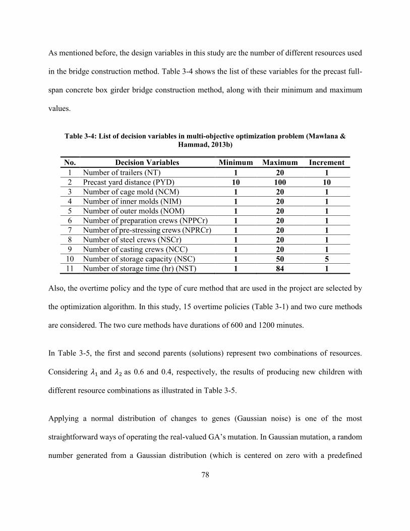
78

As mentioned before, the design variables in this study are the number of different resources used

in the bridge construction method. Table 3-4 shows the list of these variables for the precast full-

span concrete box girder bridge construction method, along with their minimum and maximum

values.

Table 3-4: List of decision variables in multi-objective optimization problem (Mawlana &

Hammad, 2013b)

No. Decision Variables Minimum Maximum Increment

1 Number of trailers (NT) 1 20 1

2 Precast yard distance (PYD) 10 100 10

3 Number of cage mold (NCM) 1 20 1

4 Number of inner molds (NIM) 1 20 1

5 Number of outer molds (NOM) 1 20 1

6 Number of preparation crews (NPPCr) 1 20 1

7 Number of pre-stressing crews (NPRCr) 1 20 1

8 Number of steel crews (NSCr) 1 20 1

9 Number of casting crews (NCC) 1 20 1

10 Number of storage capacity (NSC) 1 50 5

11 Number of storage time (hr) (NST) 1 84 1

Also, the overtime policy and the type of cure method that are used in the project are selected by

the optimization algorithm. In this study, 15 overtime policies (Table 3-1) and two cure methods

are considered. The two cure methods have durations of 600 and 1200 minutes.

In Table 3-5, the first and second parents (solutions) represent two combinations of resources.

Considering 𝜆1 and 𝜆2 as 0.6 and 0.4, respectively, the results of producing new children with

different resource combinations as illustrated in Table 3-5.

Applying a normal distribution of changes to genes (Gaussian noise) is one of the most

straightforward ways of operating the real-valued GA’s mutation. In Gaussian mutation, a random

number generated from a Gaussian distribution (which is centered on zero with a predefined

79

standard deviation) is added to each gene (real number). The new mutated gene is then replaced in

the chromosome (Hinterding, 1995). The uniform distribution (UD) is another mutation method

used in real-valued GAs (Iba & Noman, 2012).

Table 3-5: Arithmetic crossover operator for real-valued GAs

Decision Variables Parent 1 Parent 2 Child 1 Child 2

Number of trailers (NT) 2 4

3 3

Precast yard distance (PYD) 20 60 36 44

Number of cage mold (NCM) 6 15 10 11

Number of inner molds (NIM) 6 8 7 7

Number of outer molds (NOM) 5 15 9 11

Number of preparation crews (NPPCr) 1 1 1 1

Number of pre-stressing crews (NPRCr) 1 1 1 1

Number of steel crews (NSCr) 5 8 6 7

Number of casting crews (NCC) 2 2 2 2

Number of storage capacity (NSC) 25 40 31 34

Number of storage time (hr) (NST) 15 13 14 14

3.5 Parallel Computing Approach

Large number of resources required in complex and large scale construction projects, such as

bridge construction processes results in a very large search space. Therefore, due to the huge

number of calculations resulting from this large search space, multiple objective functions, large

number of replications performed in the stochastic simulation model, and the lack of the GA ability

in fast convergence to the optimum results in complex and large scale construction projects, there

is a need for parallel computing in order to reduce the computational time. According to the

Section 2.10, the master-slave (or global) parallelization and coarse-grained parallel GAs are two

main parallel paradigms usually used when solving an optimization problem in order to improve

the performance of the solver. In this research, the former is used as a parallel computing technique

to decrease the computation time and to efficiently use the full capacity of the computer as shown

in Figure 3-10.

𝜆 1=

0.6

& 𝜆

2=

0.4

80

There are basically three important terms in parallel computing that should be defined and

distinguished carefully. These terms are node, CPU, and core. A node is an object within a

network, such as several nodes available within a cluster system. CPU is an execution part of a

computer that performs software programs. Cluster systems may have many CPUs in each node.

An individual processor of a computer that actually performs programs called core. Usually, each

CPU has one core in desktop computers; however, in a cluster each CPU may contains many cores

which is called as a multiprocessor system (Tennessee, 2014). The last two terms are

interchangeable; however, in this research the usage of these terms are based on the above

mentioned definitions.

The proposed parallel platform is implemented on two different machines: the first one is a

Server/Intel Xeon CPU E5540 @ 2.53 GHz, 48 GB Random Access Memory (RAM), running

Windows 2010 Dell computer with 12 cores and the second one is a cluster of McGill University

(Figure 3-11) with properties shown in Table 3-6. There are several number of nodes available in

this cluster that each node usually has two CPUs and each CPU contains either six or eight cores.

As mentioned in Section 2.9.1, in the global parallel GA, one of the cores works as manager

processor to create the initial population of the GA; and then, this population is divided into

subpopulations which are distributed among the remaining workers (cores).

81

Worker

Processor 3Worker

Processor 2

Worker

Processor 1

Manager

Processor

Worker

Processor N

Figure 3-10: Global parallel computing paradigm

Figure 3-11: McGill cluster (Guillimin) environment (McGill-HPC, 2014)

The variables (members) of each subpopulation are sent from the manager core to the slaves. Each

slave core then runs the simulation model and calculates the objective functions of the MOGA

(e.g., the total cost and duration of the process). Thus, the evaluation of the subpopulations is the

only parallelized operation in this parallel paradigm due to the fact that there is no dependency of

the fitness evaluation of each individual on the rest of the population (Cantú-Paz, 1998). The

communications between the workers are necessary only when the cores receive a fraction of the

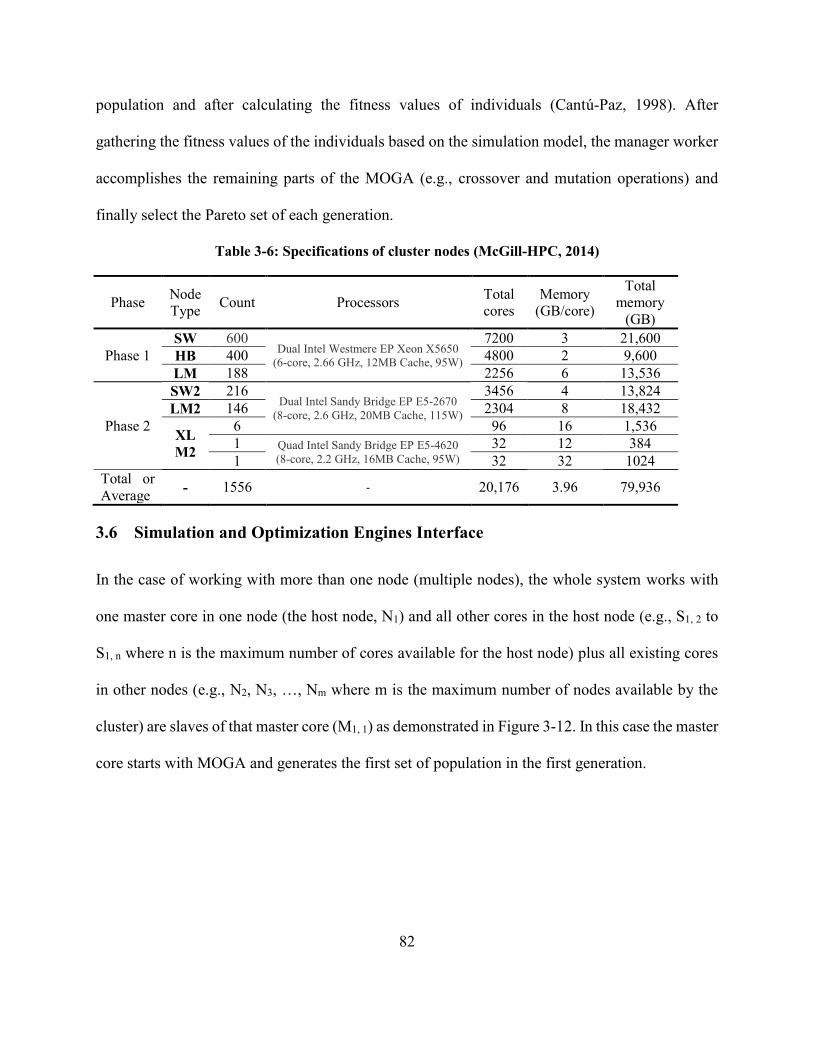
82

population and after calculating the fitness values of individuals (Cantú-Paz, 1998). After

gathering the fitness values of the individuals based on the simulation model, the manager worker

accomplishes the remaining parts of the MOGA (e.g., crossover and mutation operations) and

finally select the Pareto set of each generation.

Table 3-6: Specifications of cluster nodes (McGill-HPC, 2014)

Phase Node

Type Count Processors

Total

cores

Memory

(GB/core)

Total

memory

(GB)

Phase 1

SW 600 Dual Intel Westmere EP Xeon X5650

(6-core, 2.66 GHz, 12MB Cache, 95W)

7200 3 21,600

HB 400 4800 2 9,600

LM 188 2256 6 13,536

Phase 2

SW2 216 Dual Intel Sandy Bridge EP E5-2670


3456 4 13,824

LM2 146 2304 8 18,432

XL

M2

6 96 16 1,536

1 Quad Intel Sandy Bridge EP E5-4620


32 12 384

1 32 32 1024

Total or

Average - 1556 - 20,176 3.96 79,936

3.6 Simulation and Optimization Engines Interface

In the case of working with more than one node (multiple nodes), the whole system works with

one master core in one node (the host node, N1) and all other cores in the host node (e.g., S1, 2 to

S1, n where n is the maximum number of cores available for the host node) plus all existing cores

in other nodes (e.g., N2, N3, …, Nm where m is the maximum number of nodes available by the

cluster) are slaves of that master core (M1, 1) as demonstrated in Figure 3-12. In this case the master

core starts with MOGA and generates the first set of population in the first generation.

83

Nm N3First Node, N1 (Host Node)

Master Core,

M1,1

Slave

Core, S1,2

Slave

Core, S1,3

Slave

Core, S1,4

Slave

Core,

S1,11

Slave

Core, S1,n

Seconed Node, N2

Slave

Core, S2,2

Slave

Core, S2,3

Slave

Core, S2,n

Slave

Core, S2,1

Figure 3-12: Schematic communication between multiple nodes

Then, this population will be divided into subpopulations based on the number of available slave

cores. The variables of the members of each subpopulation are sent from the master core to the

slaves and each slave core runs the simulation model to calculate the objective functions of the

MOGA (e.g., the total cost and duration of the process). The output results of the simulations (i.e.,

the fitness values of the members of the subpopulations) are sent back to the master core in order

to perform crossover and mutation operations and finally select the Pareto set of the first

generation. Therefore, both interactions between cores (represented by bidirectional arrows in the

above figure) are through MATLAB variables. In the second generation, the master core generates

a new set of population and the whole procedure is repeated again until the maximum number of

generations is reached.

3.7 Sensitivity Analyses

3.7.1 Effect of GA Parameters

Translating a problem to the GA, defining the fitness function(s) for the problem, and setting the

GA parameters are the three main components in the design procedure of the GAs (Wu et al.,

84

2012). The focus of this part of the research is on the third component. Population size, number of

generations, the operators’ parameters (i.e., crossover probability, mutation probability, etc.),

stopping criteria, etc. are some instances of the GA parameters.

The main goal of applying sensitivity analysis is to identify the most and less influential input

parameters on the GA performance for the specific simulation-based optimization problem used

in this research. In order to achieve this goal, the effect of three main parameters of NSGA- are

investigated by varying one parameter each time while fixing the others. Population size, number

of generations, and crossover probability are the three main parameters for checking the sensitivity

of the final outputs (i.e., quality of the objective functions) against the variations in their values.

The GA is then tuned based on the best obtained parameters which maximize the GA’s

performance (Sugihara, 1997).

The number of individuals created randomly for exploring the whole search space as much as

possible in each generation is called the population size (Sivanandam & Deepa, 2008). The GA

ability to find the global optimum results instead of local ones mainly depends on the population

size of the GA (Iba & Noman, 2012). However, the complexity of each problem determines the

population size of the GA, the larger population size results in more diversity of points in the

search space which leads to better and more optimized results. On the other hand, when the size

of population increases, it takes more time and memory for the GA to converge. Practically, the

population size of around 100 is common for different purposes which can be changed based on

the required balance between the time and memory of the computer and the quality of the final

solutions (Sivanandam & Deepa, 2008; Kamil et al., 2013).

85

The number of generations is another important factor when using the GA. The number of

generations can vary for each problem; however, the range of 50 to 500 generations is typically

used for the GA optimization problems (Mitchell, 1998).

According to Section 3.4, the crossover probability (𝑃𝑐) in each generation specifies the percentage

of the total population which goes through the crossover operation to produce new children from

the parents of the previous generation. There are different ranges suggested for this parameter by

researchers. For example, Roeva (2008) used the range of [0.5, 1] with an interval of 0.1 for her

experiments. Several researches demonstrated that the best crossover probability suggested values

are between 0.7 and 1 (mostly around either 0.7 or 0.8) (Sugihara, 1997; Kamil et al., 2013; Roeva

et al., 2013).

3.7.2 Effect of Number of Cores

The performance of the proposed parallel platform is compared with respect to the computation

time. The time which is needed to reach to the final near optimum results using the proposed

framework is calculated for different numbers of cores. For this purpose, all tests took place on the

above mentioned server machine with Windows 2010 Professional operating system and the

McGill University cluster (Guillimin) within the MATLAB R2014a environment. The calculation

is done for both the deterministic and probabilistic simulation-based optimization models by

assigning deterministic and random distributions to the activities’ durations, respectively.

3.8 Comparison of Different Pareto Fronts

As mentioned in Section 2.8, MOGAs generate a set of optimum solutions instead of one optimal

answer as in the case of single objective optimization methods. This causes decision makers to

86

face with some troubles finding the best optimum set of solutions when there are more than one

Pareto front for a problem, since it is difficult to compare the Pareto fronts that are not definitely

dominated by one of them; especially when they intersect with each other (Figure 3-13). In order

to alleviate this limitation, many indicators have been introduced which enable easy comparison

of Pareto fronts from the point of view of the quality of the optimum solutions, by converting a set

of optimum solutions to a single value (Bradstreet, 2011; Zitzler et al., 2003).

The hypervolume indicator (also known as Lebesgue measure (Laumanns et al., 2000) or S-metric

(Fleischer, 2003; Purshouse, 2003; Zitzler, 1999) is one of the most popular indicators for multi-

objective evolutionary algorithms. The hypervolume indicates the dominated space (i.e., area or

volume for two objectives and three objectives optimization problems, respectively) between the

optimum sets and a reference point. The larger the hypervolume, the better the set of optimum

solutions, since it indicates that either the Pareto front is more toward the origin or it has more

diversity in optimum solutions in comparison with the other Pareto fronts (Bradstreet, 2011). Thus,

the hypervolume indicator factors in both the distance of the Pareto fronts from the best set of

optimum solutions and the diversity of the optimal solutions (Zitzler et al., 2003).

This indicator is measured relative to a selected reference point. There are different ways to choose

the proper reference point. One of the most common methods is to select the worst existing solution

among all optimal solutions (Naujoks et al., 2005; Bradstreet, 2011). Therefore, the maximum

values of each objective function (e.g., maximum cost and maximum total duration of the project

in this study) form the coordinates of the reference point in a minimization problem. For the multi-

objective optimization problems with two objective functions, the hypervolume is defined as the

87

area bounded by the selected reference point and the Pareto front’s points. Figure 3-13 shows this

dominated area.

Figure 3-13: Comparison of two intersecting Pareto fronts using Hypervolume Indicator (Adopted

from Zitzler et al., 2003)

The hypervolume indicator quantifies the performance of a set of optimum solutions in different

ways. It is used to compare the Pareto fronts after finishing the optimization procedure or it can

be used as part of the selection function within the optimization procedure to guide the search and

improve the quality of optimum solutions (Auger et al., 2009; Naujoks et al., 2005).


The needs, motivations and benefits of using the SimEvents tool to simulate the precast box girder

bridge construction processes were investigated in this chapter. Although simulating construction

processes using special purpose simulation tools is much easier to build and understand than using

SimEvents, the combination of those tools with optimization tools is difficult and an integration

88

platform is needed. The benefits reached by combining the simulation models with the

optimization technique in the same MATLAB environment were discussed, and the simulation-

based optimization framework was proposed.

The following conclusions can be stated: (1) The integration of SimEvents and NSGA- in

MATLAB made it possible to export the simulation results of the simulation-based MOGA for

precast box girder bridge construction processes to a shared workspace and linking them with the

optimization module without the need for developing an interface or integration programming; (2)

integrating the simulation-based optimization in a single environment, that supports parallel

computing and runs on a cluster, results in reducing the computation time in comparison with the

conventional integration solutions; and (3) The factors that affect the performance of the

simulation-based MOGA were identified along with the hypervolume method for comparing the

Pareto fronts as will be discussed in Chapter 4.

89

CHAPTER 4 IMPLEMENTATION AND CASE STUDY

4.1 Introduction

The implementation of the proposed HPC parallel simulation-based optimization framework is

investigated in this chapter to highlight the strengths of the proposed method. Also, a hypothetical

case study is considered to demonstrate the feasibility of the developed models, and to analyze the

performance of the simulation model outputs in the probabilistic and deterministic modes. Finally,

HPC is applied to investigate the time saving achieved in comparison with the regular computation

methods.

4.2 Simulation Models Using SimEvents

In this research, the precast full-span concrete box girder construction method with launching

gantry which is developed before in Stroboscope in (Mawlana & Hammad, 2013b) will be used to

validate the developed MATLAB SimEvents simulation model. In addition, the precast segmental

concrete box girder construction method with launching gantry will be modeled in the simulation

tool.

4.2.1 Precast Full Span Concrete Box Girder Construction Method

4.2.1.1 SimEvents Simulation Model

The concrete bridge consists of 500 spans with identical length of 25 m. The simulation process

starts by using the resources needed for commencing the first task which is the erection of the

reinforcement and stressing ducts of the bottom slab and the webs of the full-span, and then; the

90

inner mold is installed followed by placing the reinforcement and stressing ducts of the top slab

by steel crews.

After finishing the reinforcement work, the rebar cage is put into an outer mold and the casting is

done by the casting crews. When the concrete cured and reached an acceptable strength, the inner

mold is removed. Next, the first pre-stressing procedure is performed by the pre-stressing crews

to make the full-span ready for transportation to the storage area where the full-span is completely

cured and stored (the second stage of pre-stressing process). After that, the precast full-span girder

is transported to the site by means of a trailer for erection. The trailer hauls to the position where

the onsite crane unloads the precast span from the trailer and loads it to a trolley. The trailer, then,

returns to the storage area to load another span. The girder is simultaneously delivered along the

completed part of the bridge by the trolley to its launching location where launching gantry

repositions to the location of new span.

Afterwards, the full-span is lifted from the trolley by means of the gantry's lifting frames, and the

trolley returns to be loaded again. The girder is moved forward to reach to its right position to be

placed between two piers. Then, the permanent bearings are installed to undertake the load of the

span which is transferred from the temporary bearings to the permanent bearings. In the next step,

the launcher repositions to lift the next full-span (Mawlana & Hammad, 2013b). Figure 4-1

illustrates the developed SimEvents simulation model of bridge construction using precast full-

span launching method.

91

4.2.1.2 Stroboscope Simulation Model

The Stroboscope simulation model of the bridge construction using precast full span launching

method is developed in (Mawlana & Hammad, 2013b) and is shown in Figure 4-2.

4.2.2 Validation of Full Span Simulation Model (Deterministic Mode)

In order to validate the deterministic SimEvents simulation model of the precast full-span concrete

box girder construction method with launching gantry, the durations of different activities of the

simulation model are considered deterministic (fixed numbers) since the deterministic model is

easier to build to approximate the reality (Appendix A).

Table 4-1 illustrates the fixed durations of the deterministic simulation model’s activities. For

different combinations of resources, simulation models are run with SimEvents and Stroboscope,

and in the next step the results of the two models are compared as shown in Table 4-2. As obvious

from this table, there is no difference between the results of two models for all considered

combinations of the resources.

4.2.3 Validation of Full Span Simulation Model (Probabilistic Mode)

In the next step, the probabilistic simulation model was built by assigning random distributions to

the activities’ durations to consider uncertainty associated with the construction processes. The

random distributions of activities durations are presented in Table 4-3. Thus, every time the model

is run, a different set of outputs is obtained due to distinct seed numbers generated for each run of

the simulation model.

92

Storage-Cap Queue

Rebar-Mold Queue

Spans Queue

Steel Crew Queue

Bottom Slab-Web

Inner Mold Queue Cast Crew Queue

Inner Mold Top Slab Lift To Mold

SteelCr in

SteelCr outSteelCr in

SteelCr out

InM in

Prep Crew Queue

PrCr outPrCr in

Remove Inner Mold

PrCr outPrCr in

Lift To Storage

OuM out

Outer Mold Queue OuM in

Cast Span

YrC inYrC out

RM in

RM out

Span CuringPosttension_1st

Stressing Crew Queue

StressCr outStressCr in

Posttension_2nd

StressCr outStressCr in

YardCrane_1 Queue

YrC outYrC in

Storage Time

Yard Crane Queue

Trailer Loading

SC in

SC out

Trailer Haul Trolley Loading

Onsite Crane Queue

Onsite Trolley Queue Trolley in

Trolley Return and Erect Span

Trolley Travel and

Trailer ReturnReposition

Ready Queue

Trolley out

Trailer Queue

Ready out

Pickup Span

Launching Gantry Queue

Prepare BearingLoad Transfer

Ready in

Entity Sink

Figure 4-1: Simulation model of bridge construction using precast full-span launching method

93

Yard_Cra

ne

Loading_

Ready

Trailer_Loadin

gPS12

DT1

LC1 LC2

Trailer_Haul

Trailer_ReturnDT6

DT2Unloadin

g_Read

Trolley_Loadin

g

Onsite_Tr

olley

Onsite_C

rane

Trolley_Travel

DT3 DT4

OC1 OC2

OT1

DT5

OT2

Launch_

ReadyOT3OT4

OT5

Erect_SpanPrepare_Beari

ngLG2LG3PS13

Launch_

Gantry

LG5

LG1Trolley_Return

OT6

Placed_S

pans

PS15

Pickup_Span Reposition

Cast_SpanSpan_CuringSpan_Re

ady

Prep_Cre

w

Steel_Cre

w

BottomSlab_W

eb

ST1

Bottom_R

eadySC2

ST2

Rebar_M

oldCA1

Inner_MoldSC3

PC1 PC2

Top_Rea

dySC4 TopSlab

ST4

SC5CageRea

dySC6

LiftToMold

SC7

CA2

ST3

Outer_Mo

ldOM1

CastRead

ySC8SC9PS1PS2

RemoveInner

Mol

PS3

Postensio

nReadyPS4

InnerMold

IM1

IM2

Posttension_1

stPS5

Store_Re

adyPS6LiftToStorage PS7

Posttensi

oReadyPS8

Posttension_2

ndPS9

Site_Tran

sport

PS10

OM2

Stressing

_Crew

PR1PR2

PR3 PR4

PC3

PC4

YardCran

e_1

YC1YC2

YC3YC4

Spans_R

equired

PS00

Cast_Cre

w

CC1 CC2

PC3

PC4ST4 ST3

CA2

PS11

PR3PR4

IM2

OM2

PS3

YC2 YC1

Casting Operation

Launching Operation

Load_Transfer PS14

RE2

Storage_

Cap

CP1

CP2

CP2

Storage_Time

Ready

RE1

Figure 4-2: Simulation Model of Bridge Construction Using Full Span Launching Method

(Mawlana & Hammad, 2013b)

Table 4-1: Activities durations for deterministic simulation model

Activity Duration (minutes) Activity Duration (minutes)

BottomSlab_Web 1673 * Trailer_Loading 60 **

Inner_Mold 300 * Trailer Haul F (Distance, Speed)

TopSlab 1979 * Trolley_Loading 60 **

LiftToMold 45 Trailer_Return F (Distance, Speed)

Cast_Span 1544* Trolley_Travel F (Distance, Speed)

Span_Curing (600 or 1200) * Reposition 240 **

RemoveInnerMol 255 * Erection_Span 240 **

Posttension_1st 240 * Trolley_Return F (Distance, Speed)

LiftToStorage 60 ** Prepare_Bearing 240 **

Posttension_2nd 240 * Load_Transfer 60 **

* Adapted from (Marzouk, El-Dein, & El-Said, 2007)

** Adapted from (VSL International Ltd, 2013)

94

Table 4-2: Comparison of the total duration and cost of the deterministic simulation models with

SimEvents and Stroboscope

Decision Variables First Set Second Set Third Set

Number of trailers (NT) 1 2 4

Precast yard distance (km) (PYD) 10 10 60

Number of cage mold (NCM) 1 2 1

Number of inner molds (NIM) 1 2 1

Number of outer molds (NOM) 1 2 2

Number of preparation crews (NPPCr) 1 4 6

Number of pre-stressing crews (NPRCr) 1 4 6

Number of steel crews (NSCr) 1 4 6

Number of casting crews (NCC) 1 4 6

Number of storage capacity (NSC) 1 10 50

Number of storage time (hr) (NST) 1 10 50

Overtime Policy (OP) 1 2 4

Duration of cure method (DCM) 1 2 2

Objective Functions

Duration (days) (SimEvents) 1751.67 487.31 627.92

Duration (days) (Stroboscope) 1751.67 487.31 627.92

Cost (M$) (SimEvents) 1462.86 1568.44 2650.31

Cost (M$) (Stroboscope) 1462.86 1568.44 2650.31

Also, in order to assess the risk associated with the construction processes, replications were

performed. The concept of replications is based on running the simulation model for a large

number of times (for example 1000 times); and therefore, each replication will have different

performance outcomes (in this case, total duration and cost of the project) (Nelson et al., 2013).

For different combinations of resources, simulation models are run with SimEvents (Appendix B)

and Stroboscope, and in the next step the results of the two models are compared as shown in

Table 4-4. As obvious from this table, there are either very small or no differences between the

results of two models for all three combinations of the resources. Selection of different seed

numbers by two simulation tools for each run of the simulation models in the probabilistic mode

results in small differences in some set of resources combinations.

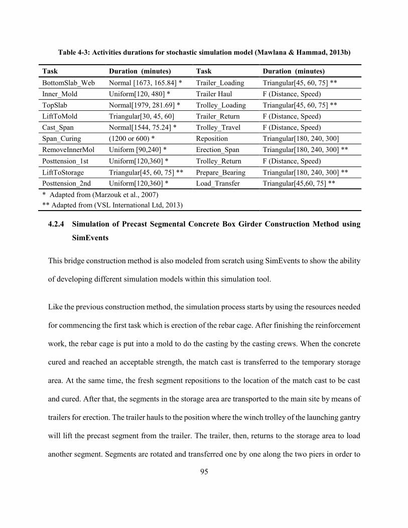
95

Table 4-3: Activities durations for stochastic simulation model (Mawlana & Hammad, 2013b)

Task Duration (minutes) Task Duration (minutes)

BottomSlab_Web Normal [1673, 165.84] * Trailer_Loading Triangular[45, 60, 75] **

Inner_Mold Uniform[120, 480] * Trailer Haul F (Distance, Speed)

TopSlab Normal[1979, 281.69] * Trolley_Loading Triangular[45, 60, 75] **

LiftToMold Triangular[30, 45, 60] Trailer_Return F (Distance, Speed)

Cast_Span Normal[1544, 75.24] * Trolley_Travel F (Distance, Speed)

Span_Curing (1200 or 600) * Reposition Triangular[180, 240, 300]

RemoveInnerMol Uniform [90,240] * Erection_Span Triangular[180, 240, 300] **

Posttension_1st Uniform[120,360] * Trolley_Return F (Distance, Speed)

LiftToStorage Triangular[45, 60, 75] ** Prepare_Bearing Triangular[180, 240, 300] **

Posttension_2nd Uniform[120,360] * Load_Transfer Triangular[45,60, 75] **

* Adapted from (Marzouk et al., 2007)

** Adapted from (VSL International Ltd, 2013)

4.2.4 Simulation of Precast Segmental Concrete Box Girder Construction Method using

SimEvents

This bridge construction method is also modeled from scratch using SimEvents to show the ability

of developing different simulation models within this simulation tool.

Like the previous construction method, the simulation process starts by using the resources needed

for commencing the first task which is erection of the rebar cage. After finishing the reinforcement

work, the rebar cage is put into a mold to do the casting by the casting crews. When the concrete

cured and reached an acceptable strength, the match cast is transferred to the temporary storage

area. At the same time, the fresh segment repositions to the location of the match cast to be cast

and cured. After that, the segments in the storage area are transported to the main site by means of

trailers for erection. The trailer hauls to the position where the winch trolley of the launching gantry

will lift the precast segment from the trailer. The trailer, then, returns to the storage area to load

another segment. Segments are rotated and transferred one by one along the two piers in order to

96

place them in their right position. After reaching to the adequate number of segments to form a

full span, pre-stressing crews fix the segments by using temporary fixing materials. When a full

span is made from connected segments, post tensioning is applied by pre-stressing crews. The

temporary fixing bars are removed simultaneously. Then, the load of the span is transferred from

the launching girder to the piers. In the next step, the launcher repositions to lift the next set of

segments, and the process repeats again. The developed simulation model of bridge construction

using precast segmental launching method is shown in Figure 4-3.

4.3 Integration of MATLAB MOGA Optimization Tool and SimEvents Simulation

Model

The MOGA optimization initializes by generating the first set of population using the default

defined function in MATLAB using a uniform random number generator. The variables’ upper

and lower bounds are defined as a matrix with two rows and the number of columns equals to the

number of variables. If the defined matrix has one row and two columns, then all the variables

have the same range. The default values for the upper and lower bounds are zero and one,

respectively.

This means that the maximum and minimum values for the all variables are one and zero,

respectively. As shown in Table 3-4, the bounding matrix in this study is defined as follow:

Bounding Matrix = [ 1 10 1 1 1 1 1 1 1 1 1 1 1

] 20 100 20 20 20 20 20 20 20 50 84 15 2

The main code of applying NSGA- within the integrated proposed framework as well as all other

required functions within the optimization algorithm are shown in Appendices C and D,

respectively.

97

Storage-Cap Queue

Rebar-Mold Queue

Segments Queue

Steel Crew Queue

Rebar Cage

Cast Crew Queue

Lift To Mold

Lift Segment To

Storage

Mold Queue MO in

Cast SegmentRM in

RM out

Segment Curing

Reposition of Fresh

Segment

MO out

YardCrane_1 Queue

Storage Time

Yard Crane Queue

Trailer Loading

SC in

Trailer Haul Pickup Segment

Onsite Crane Queue

Winch Trolley Queue Trolley in

Segment Rotation

and TransferConsolidadtion

Prep Crew Queue

Trailer Queue

Temporary Fixing

Load TransferEntity Sink

Trailer Return

Posttensioning

Stressing Crew Queue

PrCr outPrCr in

Remove Temporary Fixing

PrCr out PrCr in

Launching Gantry Queue Reposition LG out

LG in

Figure 4-3: Simulation model of bridge construction using precast segmental launching method

98

Table 4-4: Comparison of the total duration and cost of the probabilistic simulation models with SimEvents and Stroboscope

Decision Variables First Set Second Set Third Set

Number of trailers (NT) 9 7 8

Precast yard distance (km) (PYD) 28 30 34

Number of cage mold (NCM) 11 8 10

Number of inner molds (NIM) 12 10 11

Number of outer molds (NOM) 9 9 8

Number of preparation crews (NPPCr) 3 2 3

Number of pre-stressing crews (NPRCr) 10 2 3

Number of steel crews (NSCr) 11 5 7

Number of casting crews (NCC) 7 4 5

Number of storage capacity (NSC) 31 27 23

Number of storage time (hr) (NST) 85 47 44

Overtime Policy (OP) 6 1 6

Duration of cure method (DCM) 2 1 2

Objective Functions Differences Differences Differences

Duration (days) (SimEvents) 482 0%

1261 0.32%

484 0%

Duration (days) (Stroboscope) 482 1257 484

Cost (M$) (SimEvents) 17810 0.067%

2200 0%

11883 0.03%

Cost (M$) (Stroboscope) 17798 2200 11887

99

According to Section 3.6, the simulation-based optimization framework works with one master

core in one node (the host node) and all other cores in the host node and other nodes are slaves of

that master core. After dividing the population into subpopulations based on the number of

available slave cores, there is a need to transfer the variables of each subpopulation from the master

core to the slaves. In MATLAB environment, this transition is performed using “set_param”

command (Appendices A and B). This command sets the selected values of the simulation model

variables (resource combinations) by the GA within the simulation model. Each slave core then

runs the simulation model and calculates the objective functions of the MOGA (i.e., the total cost

and duration of the process).

The output results of the simulations (the fitness values of the members of the subpopulations) are

sent to the master core in order to perform crossover and mutation operations. The non-dominated

rank and distance measure of the individuals are used to produce the next generation of population

to finally reach to the set of optimal trade-off solutions known as the Pareto front. The relative

fitness of each individual determines the non-dominated rank of that individual. When solution p

has better value in at least one objective function in comparison with solution q, it has lower rank

than q and it dominates solution q. The distance measure of a solution is used when two solutionss

have equal ranks; thus, neither one dominates the other (Bradstreet, 2011; Zitzler et al., 2003).

As mentioned in Section 3.5, global parallel GA is used in this research to decrease the

computation time and to efficiently use the full capacity of the computer due to the huge number

of calculations resulting from the large search space, multiple objective functions, and large

number of replications performed in the stochastic simulation model. Regarding running

SimEvents simulation model in the parallel mode, the SIM command is used to run the simulation

100

model, and enclose this command within a PARFOR loop to perform the replications. A PARFOR

loop is useful in situations where there are many loop iterations of a simple calculation, such as a

Monte-Carlo simulation, DES or doing replications. PARFOR divides the group of loop iterations

into subgroups, so that each worker (core) executes a portion of the total number of iterations.

PARFOR loops are also useful when there are loop iterations that take a long time to execute,

because the workers can execute iterations simultaneously (Appendices A and B). After having

done the number of replications required, the mean values of the objective functions are calculated

as final solutions.

4.4 Validation of the Proposed Optimization Model using Full Span Construction

Method

The proposed integrated simulation-based optimization model is validated by comparing the

optimal solutions obtained from NSGA- optimization algoritm with those obtained from fast

messy GA (fmGA) which is another type of GAs (Mawlana & Hammad, 2013b).

Like the proposed MOGA, fmGA works based on the main principles of the simple GA with some

modifications to alliviate the shortcomings of the messy GA and the simple GA. The fmGA

consists of two loops called the inner and outer loops. Each outer loop, which is also called an era,

perfoms an inner loop. The optimization starts with the random generation of the initial population

within the inner loop. Then, the optimal solutions are evalutaed based on their fitness values and

some selection and filtering processes (i.e., cut and splice, mutation) are applied on these solutions

to increase the probability of finding the better solutions in the next generation. Finally, the

optimization procedure stops when the termination critera are reached (Goldberg et al. 1993).

101

Figure 4-4 compares the Pareto solutions attained by the proposed multi-objective NSGA- and

by the fmGA (Mawlana & Hammad, 2013b). In order to compare under the same main parameters,

the number of generations and the size of the population are set to 2000 and 100, respectively, for

both algorithms. In some cases, the two optimization algorithms produce almost close optimum

solutions in terms of the project cost and duration as shown in Figure 4-4. However, the fmGA

overall generates more costly and more time consuming optimum solutions in comparison with

NSGA-. For example, there are 5% and less than 1% differences between the best optimum

solutions obtained by the fmGA and NSGA- from cost and time points of view, respectively.

Also, there are almost 11% and 1% decrement in terms of the average project cost and duration in

the solutions generated by NSGA- in comparison with those generated by fmGA, respectively.

The hypervolume indicator is also used to compare the two Pareto sets by mesuring the dominated

area of each Pareto set according to a selected reference point (Zitzler & Thiele, 1999). This

comparison results in 19.41% and 18.72% of the hypervolume indicator for the fronts generated

by NSGA- and fmGA, respectively. The larger hypervolume indicator of NSGA- indicates the

better performance of this optimization algorithm in comparison with the fmGA from quality of

solutions point of view. In addition, the total time required to complete the run of the proposed

framework using NSGA- and fmGA was 5.33 and 11.2 hours, respectively. These results

demonstrate the better performance of NSGA- in comparison with the fmGA from computation

time point of view. However, it is important to note that two mentioned algorithms were run on

two different machines with different properties (i.e., different number and type of cores).

Integrated simulation model with NSGA- algorithm was run on one node of a cluster system with

12 cores and Dual Intel Westmere EP Xeon X5650 property; however, 4-core machine with Intel

102

Core (TM) i7-2600 was used to run the fmGA. These differences affect the required computation

time.

4.5 Sensitivity Analyses on the Server Machine

As stated in Section 3.7, the main goal of applying sensitivity analysis is to identify the most and

less influential input parameters on the GA performance. Population size, number of generations,

and crossover probability are the three main parameters for checking the sensitivity of the final

outputs (i.e., quality of the objective functions) against the variations in their values. The outcome

of this analysis is expected to provide a better understanding of how changes in the various

parameters of GA affect the total cost and duration of the construction project.

Figure 4-4: Comparison of Pareto solutions obtained from NSGA- and fmGA (results of fmGA

are adapted from (Mawlana & Hammad, 2013b))

1500

2000

2500

3000

3500

4000

4500

850 950 1050 1150 1250 1350

CO

ST

(M

$)

DURATION (DAYS)

Pareto Front-NSGA II

Pareto Front- fmGA

103

In order to perform the sensitivity analysis, uniform random number generator, arithmetic

crossover, and Gaussian mutation are considered as the creation, crossover, and mutation

functions, respectively. In the first phase of performing sensitivity analysis (phase I), the

configuration ranges considered for the number of generations and size of the population of

optimization algorithm are given in Table 4-5.

Also, according to the random nature of the used MOGA algorithm five runs of NSGA- are

performed for each case of the sensitivity analysis to ensure the consistency of the results. The

final results are the average values of solutions obtained from those five runs. Considering these

ranges, phase I results in 80 combinations.

Table 4-5: List of NSGA-𝚰𝚰 Parameters (Phase I)

NSGA-𝚰𝚰 Parameters Range

Number of Generations 500 1000 2000 4000

Size of Population 50 100 200 400

After determining the best number of generations and the best size of population based on the

results from the phase I of the sensitivity analysis (considering both the quality of the optimal

solutions and the time required to reach to those solutions), the second phase of sensitivity analysis

(phase II) is conducted. Table 4-6 shows the ranges considered for the remaining parameter of

NSGA-ΙΙ (e.g., crossover probability).

Table 4-6: List of NSGA-𝚰𝚰 Parameters (Phase II)

NSGA-𝚰𝚰 Parameters Minimum Maximum Increment

Crossover Probability 0.5 1 0.1

104

The crossover and mutation probabilities are depended on each other in NSGA-ΙΙ which means

the summation of these two probabilities is always equal to one. For example, if the crossover

probability is selected as 0.7, the mutation probability is automatically set as 0.3. Therefore,

finding the best crossover probability results in determination of the best mutation probability as

well.


4.5.1.1 Effect of Population Size

The MOGA used by MATLAB considers ‘15*numberOfVariables’ as a default value for the

population size which may not be very accurate for problems with large number of variables

(MathWorks, 2013a). Note that there are 13 decision variables defined in the proposed framework,

the default value for the population size is 195. This number can be changed and specified within

either the MOGA script (command line) or the Optimization app in Global Optimization Toolbox

of MATALB. In this study, the number of generations are fixed to 500, 1000, 2000 and 4000 for

each set of population size of 50, 100, 200 and 400.

As shown in Figure 4-5, for the number of generations of 500, almost the same optimal solutions

are produced by population size of 50 and 100. However, by increasing the population size to

either 200 or 400 the quality of solutions is improved; hence, the best optimum solutions are

obtained for higher size of population. According to Section 3.8, the hypervolume of the Pareto

fronts is calculated to show the dominated area bounded between the Pareto front points and the

reference point (Table 4-7). In order to calculate the hypervolume for these four Pareto fronts, the

reference point is selected based on the maximum value of both objective functions in all fronts.

105

This results in the reference point with the coordinates of 1248 (days) and 4289 (M$). These

coordinates belong to the Pareto front with the population size of 50 which has the highest total

duration and cost of the project among the remaining Pareto fronts. All the hypervolumes are

calculated based on the area dominated between this reference point and the Pareto front’s points

and are shown in percentage (Appendix E).


These percentages indicate the ratio of the dominated area between the reference point and each

Pareto front to the area bounded between the reference point and the origin (Figure 3-13). In order

to compare the hypervolume percentages, the normalized value of those are also calculated by

dividing each hypervolume by the maximum hypervolume percentage (Table 4-7). As

demonstrated in this table, population sizes of 200 and 400 generate the Pareto fronts with the

hypervolume of 16.11% and 15.87%, respectively. This means that the optimum solutions

1400

1900

2400

2900

3400

3900

4400

850 900 950 1000 1050 1100 1150 1200 1250

CO

ST

(M

$)

DURATION (DAYS)

NDP-Pop50

NDP-Pop100

NDP-Pop200

NDP-Pop400

106

generated by 400 population are very similar to those obtained from population size of 200.

Therefore, considering the extra computational burden imposed to the system by doubling the size

of population, 200 seems to be the promising population size for the fixed 500 generations. The

larger hypervolume indicates that either the Pareto front is closer to the origin (better convergence)

or has more diversity of the optimum solutions (wider Pareto front).

Figure 4-6: Reference point for average Pareto solutions for different population sizes with 500

generations

The proposed framework is also tested for various population sizes when the number of

generations is fixed to 1000, 2000 and 4000. The results are illustrated in Figure 4-7, Figure 4-8

and Figure 4-9, respectively. For the number of generations to 1000 (Figure 4-7), the optimum

results are close to each other for various sizes of population. While, considering the results of the

hypervolume calculation (Table 4-7) indicates that the best optimum solutions generated by 200

1400

1900

2400

2900

3400

3900

4400

850 900 950 1000 1050 1100 1150 1200 1250

Co

st (

M$

)

Duration (days)

NDP-Pop50

NDP-Pop100

NDP-Pop200

NDP-Pop400

Reference Point = (1248, 4289)

(864, 4289)

(1248, 1743)

107

population with the hypervolume of 15.89%. The same results are achieved for the 2000

generations with the highest hypervolume for population size of 200 (20.92%) in comparison with

other sizes of population.

Table 4-7: Hypervolume percentage of the Pareto fronts produced by the fixed number of

generations (Normalized values in the lower rows)

Number of Generations Size of Population

50 100 200 400

500 13.87 14.12 16.11 15.87

86.10 87.67 100 98.51

1000 15.36 14.73 15.89 15.88

96.66 92.70 100 99.92

2000 19.72 19.00 20.92 20.76

94.27 90.85 100 99.28

4000 18.47 20.09 19.51 19.72

91.92 100 97.08 98.17

According to Table 4-7 and Figure 4-9, the quality of optimum solutions improve by almost 8%

from population size of 50 to 100 for 4000 generations. However, increasing the size of population

to 200 and 400 does not enhance the optimum solutions since the Pareto front of the population

size of 100 has the highest hypervolume among other population sizes. Thus, the 100 population

size is selected as the best size of population for the number of generations to 4000.

4.5.1.2 Effect of Number of Generations

There are three different stopping criteria in MATLAB NSGA- and the occurrence of any of

them results in stopping the GA algorithm. These criteria are the maximum number of generations

which has a default value of ‘100*numberOfVariables’, the average change in the spread of the

Pareto front with a default value of 100 (convergence criterion), and the maximum time limit in

seconds which is defined as infinity. When the value of the convergence criterion is less than the

108

specified tolerance, it means there is no improvement in the optimum solutions and the

optimization will stop since the Pareto fronts are converged (MathWorks, 2014e).


Considering 13 variables defined in the proposed framework, the default value for the number of

generations is 2600. Therefore, in order to investigate the effect of this parameter on the values of

the objective functions, this number is set to 500, 1000, 2000, and 4000. The sensitivity analysis

is performed four times by fixing the population size to 50, 100, 200 and 400.

Figure 4-10 shows the Pareto fronts obtained for the fixed population size of 50 and different

number of generations. The dominated areas between these Pareto fronts and the selected reference

point are calculated and the normalized values are shown in Table 4-8.

1400

1900

2400

2900

3400

3900

4400

850 900 950 1000 1050 1100 1150 1200 1250 1300

CO

ST

(M

$)

DURATION (DAYS)

NDP-Pop50

NDP-Pop100

NDP-Pop200

NDP-Pop400

109

Figure 4-8: Average Pareto solutions for different population sizes with 2000 generations

Figure 4-9: Average Pareto solutions for different population sizes with 4000 generations

1400

1900

2400

2900

3400

3900

4400

850 900 950 1000 1050 1100 1150 1200 1250 1300

CO

ST

(M

$)

DURATION (DAYS)

NDP-Pop50

NDP-Pop100

NDP-Pop200

NDP-Pop400

1400

1900

2400

2900

3400

3900

4400

850 900 950 1000 1050 1100 1150 1200 1250 1300

CO

ST

(M

$)

DURATION (DAYS)

NDP-Pop50

NDP-Pop100

NDP-Pop200

NDP-Pop400

110

According to Figure 4-10 and Table 4-8, there is almost 6% improvement in the quality of optimal

solutions by increasing the number of generations from 500 to 2000 for population size of 50;

however, more increase to 4000 generations make the solutions worse in most of the cases.

Therefore, 2000 generations is the best number of generations for the population size of 50 to

create optimal solutions with the hypervolume of 18.98% (the highest hypervolume among other

options).

As shown in Figure 4-11 and Table 4-8, for the fixed population size of 100, the optimum solutions

improve by increasing the number of generations to 4000 generations with more diversity of

solutions (the highest hypervolume equal to 20.72%).

Figure 4-10: Non-Dominated Pareto solutions for different number of generations with population

size of 50

1400

1900

2400

2900

3400

3900

4400

850 900 950 1000 1050 1100 1150 1200 1250

CO

ST

(M

$)

DURATION (DAYS)

NDP-Gen500

NDP-Gen1000

NDP-Gen2000

NDP-Gen4000

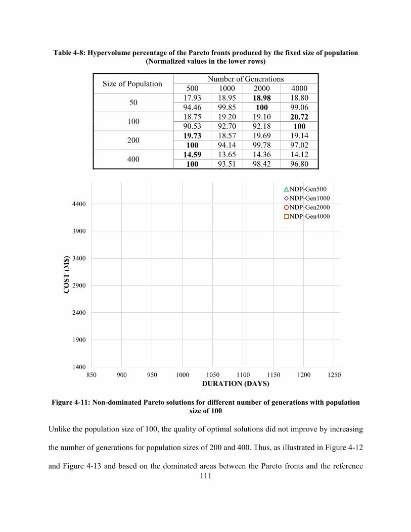
111

Table 4-8: Hypervolume percentage of the Pareto fronts produced by the fixed size of population

(Normalized values in the lower rows)

Size of Population Number of Generations

500 1000 2000 4000

50 17.93 18.95 18.98 18.80

94.46 99.85 100 99.06

100 18.75 19.20 19.10 20.72

90.53 92.70 92.18 100

200 19.73 18.57 19.69 19.14

100 94.14 99.78 97.02

400 14.59 13.65 14.36 14.12

100 93.51 98.42 96.80


size of 100

Unlike the population size of 100, the quality of optimal solutions did not improve by increasing

the number of generations for population sizes of 200 and 400. Thus, as illustrated in Figure 4-12

and Figure 4-13 and based on the dominated areas between the Pareto fronts and the reference

1400

1900

2400

2900

3400

3900

4400

850 900 950 1000 1050 1100 1150 1200 1250

CO

ST

(M

$)

DURATION (DAYS)

NDP-Gen500

NDP-Gen1000

NDP-Gen2000

NDP-Gen4000

112

points calculated in Table 4-8 the best answers are found for 500 generations. Therefore, there is

no need to increase the number of generations and impose more computation time and cost to the

system in these cases.

Table 4-9 shows the computation time needed to run the simulation-based optimization model in

deterministic mode for five times as well as the average computation time for all considered

number of generations and population sizes. These results are also illustrated in Figure 4-15 and

Figure 4-16 for fixed number of generations and fixed population sizes, respectively.

Figure 4-12: Non-dominated Pareto solutions for different number of generations with

population size of 200

According to these two figures, the required computation time is almost doubled by either making

the number of generations or the size of population double in all cases.

1400

1900

2400

2900

3400

3900

4400

850 900 950 1000 1050 1100 1150 1200 1250

CO

ST

(M

$)

DURATION (DAYS)

NDP-Gen500

NDP-Gen1000

NDP-Gen2000

NDP-Gen4000

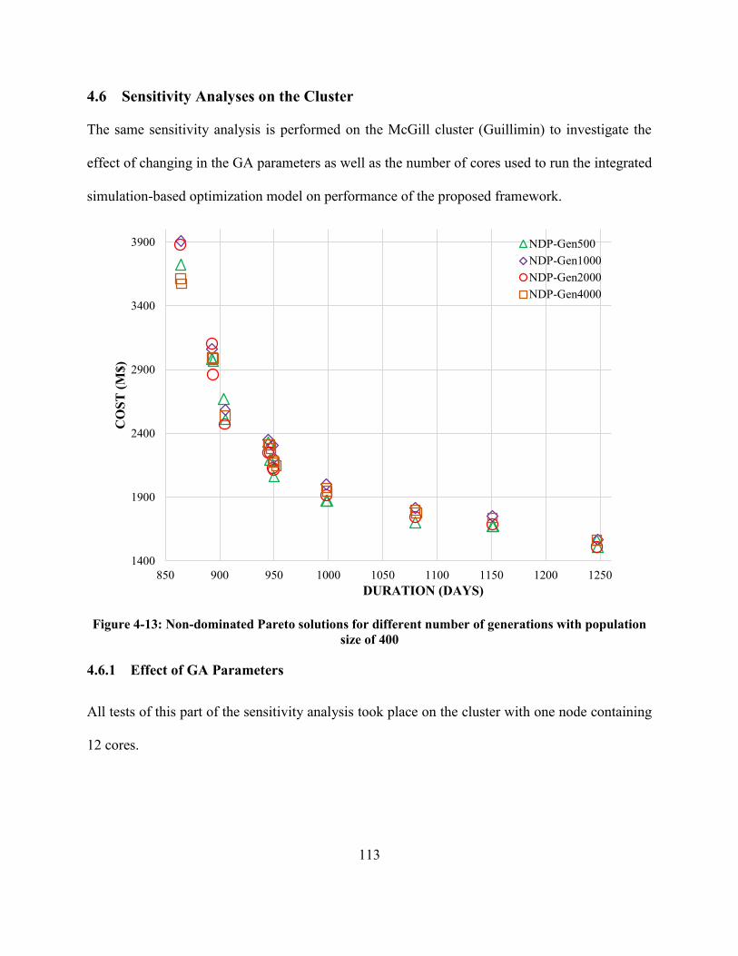
113

4.6 Sensitivity Analyses on the Cluster

The same sensitivity analysis is performed on the McGill cluster (Guillimin) to investigate the

effect of changing in the GA parameters as well as the number of cores used to run the integrated

simulation-based optimization model on performance of the proposed framework.


size of 400


All tests of this part of the sensitivity analysis took place on the cluster with one node containing

12 cores.

1400

1900

2400

2900

3400

3900

850 900 950 1000 1050 1100 1150 1200 1250

CO

ST

(M

$)

DURATION (DAYS)

NDP-Gen500

NDP-Gen1000

NDP-Gen2000

NDP-Gen4000

114

4.6.1.1 Effect of Population Size

The hypervolume of the Pareto fronts by fixing the number of generations and varying the

population size is shown in Table 4-10. Also, Figure 4-14 shows the Pareto fronts obtained for the

fixed 500 generations and different sizes of population.

Table 4-9: Computation time (min) for deterministic mode on the server machine with 12 cores

Size of

Population

Number of

Generations

Run No. Average

1 2 3 4 5

50

500 63.55 58.24 63.89 58.73 64.10 61.10

1000 119.91 118.67 118.75 118.07 117.94 118.67

2000 237.75 238.11 237.06 237.22 237.08 237.41

4000 474.18 472.82 473.38 474.61 471.78 473.35

100

500 110.40 109.30 110.10 109.31 110.15 109.85

1000 219.65 219.37 220.91 221.15 221.12 220.44

2000 443.92 441.42 446.12 441.66 440.56 442.74

4000 885.65 886.41 879.99 885.69 886.96 884.94

200

500 218.10 220.68 219.12 220.11 221.09 219.82

1000 435.65 439.83 435.91 440.50 440.43 438.46

2000 884.85 875.38 878.75 879.11 878.69 879.36

4000 1741.84 1755.78 1759.11 1756.63 1749.21 1752.51

400

500 440.37 434.62 438.51 440.02 435.90 437.88

1000 883.12 879.36 878.24 880.15 870.85 878.34

2000 1726.64 1729.73 1714.87 1718.26 1728.06 1723.51

4000 3452.94 3497.58 3451.13 3443.78 3463.69 3461.82

The population size of 400 gives the best optimum solutions which are not dominated by other sets

of optimum solutions obtained from other sizes of population based on the results shown in

Figure 4-14 and Table 4-10. The same behavior is observed for the 1000 and 2000 generations

(Figure 4-17 and Figure 4-18). Figure 4-19 illustrates the four Pareto fronts generated by 4000

generations and different number of population sizes. All the population sizes produce very similar

optimum solutions; however, the population size of 200 is the best based on the hypervolume of

the Pareto fronts calculated in Table 4-10.

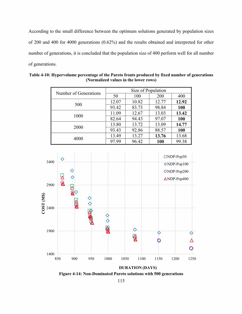
115

According to the small difference between the optimum solutions generated by population sizes

of 200 and 400 for 4000 generations (0.62%) and the results obtained and interpreted for other

number of generations, it is concluded that the population size of 400 perform well for all number

of generations.

Table 4-10: Hypervolume percentage of the Pareto fronts produced by fixed number of generations



50 100 200 400

500 12.07 10.82 12.77 12.92

93.42 83.73 98.84 100

1000 11.09 12.67 13.03 13.42

82.64 94.43 97.07 100

2000 13.80 13.72 13.09 14.77

93.43 92.86 88.57 100

4000 13.49 13.27 13.76 13.68

97.99 96.42 100 99.38

Figure 4-14: Non-Dominated Pareto solutions with 500 generations

1400

1900

2400

2900

3400

850 900 950 1000 1050 1100 1150 1200 1250

CO

ST

(M

$)

DURATION (DAYS)

NDP-Pop50

NDP-Pop100

NDP-Pop200

NDP-Pop400

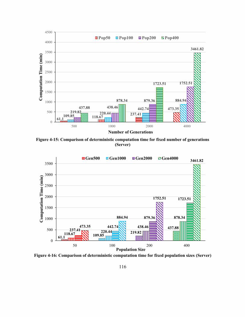
116


(Server)

Figure 4-16: Comparison of deterministic computation time for fixed population sizes (Server)

61.1118.67

237.41

473.35

109.85220.44

442.74

884.94

219.82

438.46

879.36

1752.51

437.88

878.34

1723.51

3461.82

0

500

1000

1500

2000

2500

3000

3500

4000

4500

500 1000 2000 4000

Co

mp

uta

tio

n T

ime

(min

)

Number of Generations

Pop50 Pop100 Pop200 Pop400

61.1109.85

219.82

437.88

118.67220.44

438.46

878.34

237.41442.74

879.36

1723.51

473.35

884.94

1752.51

3461.82

0

500

1000

1500

2000

2500

3000

3500

50 100 200 400

Co

mp

uta

tion

Tim

e (m

in)

Population Size

Gen500 Gen1000 Gen2000 Gen4000

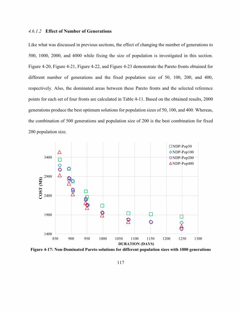
117

4.6.1.2 Effect of Number of Generations

Like what was discussed in previous sections, the effect of changing the number of generations to

500, 1000, 2000, and 4000 while fixing the size of population is investigated in this section.

Figure 4-20, Figure 4-21, Figure 4-22, and Figure 4-23 demonstrate the Pareto fronts obtained for

different number of generations and the fixed population size of 50, 100, 200, and 400,

respectively. Also, the dominated areas between these Pareto fronts and the selected reference

points for each set of four fronts are calculated in Table 4-11. Based on the obtained results, 2000

generations produce the best optimum solutions for population sizes of 50, 100, and 400. Whereas,

the combination of 500 generations and population size of 200 is the best combination for fixed

200 population size.


1400

1900

2400

2900

3400

850 900 950 1000 1050 1100 1150 1200 1250 1300

CO

ST

(M

$)

DURATION (DAYS)

NDP-Pop50

NDP-Pop100

NDP-Pop200

NDP-Pop400

118

The computation time for five deterministic runs of proposed integrated framework along with the

average computation time of those five runs are illustrated in Table 4-12. These results are also

illustrated in Figure 4-25 and Figure 4-26 for fixed number of generations and fixed population

sizes, respectively. According to these two figures, the required computation time is almost

doubled by either making the number of generations or the size of population double in all cases.


1600

1800

2000

2200

2400

2600

2800

3000

850 900 950 1000 1050 1100 1150 1200

CO

ST

(M

$)

DURATION (DAYS)

NDP-Pop50

NDP-Pop100

NDP-Pop200

NDP-Pop400

119

Table 4-11: Hypervolume percentage of the Pareto fronts produced by fixed size of population



500 1000 2000 4000

50 14.16 12.52 15.18 14.09

93.28 82.49 100 92.82

100 13.50 15.33 15.82 14.5

85.37 96.95 100 91.67

200 11.57 11.09 10.94 10.53

100 95.83 94.51 90.97

400 14.77 14.66 15.07 13.84

97.97 97.26 100 91.81


1400

1900

2400

2900

3400

3900

850 900 950 1000 1050 1100 1150 1200 1250 1300

CO

ST

(M

$)

DURATION (DAYS)

NDP-Pop50

NDP-Pop100

NDP-Pop200

NDP-Pop400

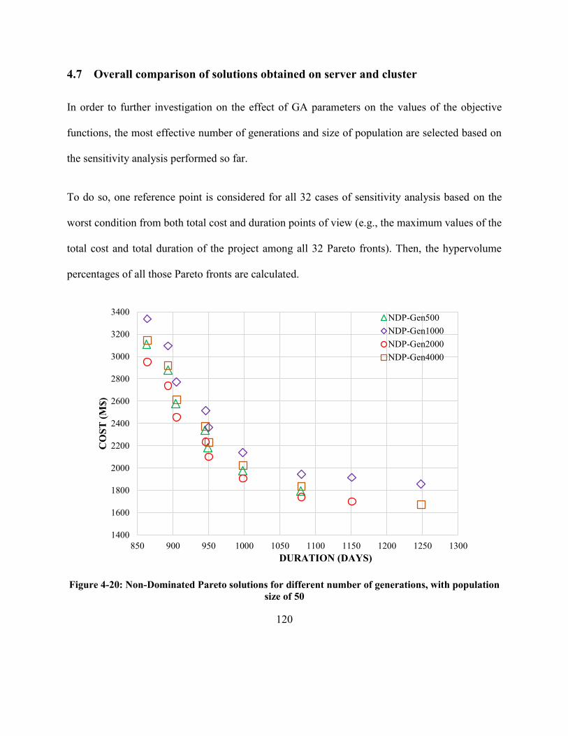
120

4.7 Overall comparison of solutions obtained on server and cluster

In order to further investigation on the effect of GA parameters on the values of the objective

functions, the most effective number of generations and size of population are selected based on

the sensitivity analysis performed so far.

To do so, one reference point is considered for all 32 cases of sensitivity analysis based on the

worst condition from both total cost and duration points of view (e.g., the maximum values of the

total cost and total duration of the project among all 32 Pareto fronts). Then, the hypervolume

percentages of all those Pareto fronts are calculated.


size of 50

1400

1600

1800

2000

2200

2400

2600

2800

3000

3200

3400

850 900 950 1000 1050 1100 1150 1200 1250 1300

CO

ST

(M

$)

DURATION (DAYS)

NDP-Gen500

NDP-Gen1000

NDP-Gen2000

NDP-Gen4000

121

Table 4-13 and Table 4-14 show the results obtained by the server machine and the cluster,

respectively. In these cases, the normalized values of the hypervolume percentages are calculated

by dividing each hypervolume by the maximum hypervolume percentage of the whole table since

they are all calculated based on the same reference point.

Table 4-12: Computation time (min) for deterministic runs on one node of the cluster with 12 cores

Size of

Population

Number of

Generations

Run No. Average

1 2 3 4 5

50

500 43.94 42.25 42.88 43.90 42.43 43.08

1000 84.80 87.05 84.71 84.66 84.62 85.17

2000 164.15 173.60 163.66 163.96 164.03 165.88

4000 326.03 327.07 328.16 329.33 323.26 326.77

100

500 77.65 82.13 82.07 82.28 83.29 81.48

1000 163.48 164.17 163.21 165.31 165.49 164.33

2000 318.56 319.21 360.45 318.09 282.06 319.67

4000 634.71 634.39 635.03 634.09 636.96 635.04

200

500 158.74 160.51 158.61 159.44 158.54 159.17

1000 311.84 311.29 311.32 316.39 310.64 312.30

2000 622.26 620.69 616.70 622.24 616.08 619.59

4000 1230.41 1232.25 1244.96 1262.71 1244.12 1242.89

400

500 309.39 311.30 314.46 311.61 309.39 311.23

1000 627.72 622.50 626.36 624.09 623.17 624.77

2000 1245.42 1243.19 1247.68 1353.75 1248.40 1267.69

4000 2510.93 2513.77 2522.82 2517.04 2500.89 2513.09

As shown in these tables, the simulation-based multi-objective optimization model is more

sensitive to the size of population since the hypervolume changes less when the number of

generations vary in comparison with the changes made by varying the size of population. As a

result, the number of generations is fixed to 500 generations. Also, considering the fact that the

hypervolume percentage of 200 and 400 population sizes are close to each other and the significant

amount of the computation time and cost imposed to the system by doubling the size of population,

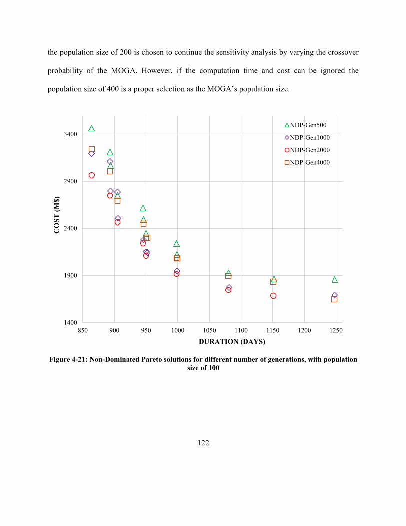
122

the population size of 200 is chosen to continue the sensitivity analysis by varying the crossover

probability of the MOGA. However, if the computation time and cost can be ignored the

population size of 400 is a proper selection as the MOGA’s population size.


size of 100

1400

1900

2400

2900

3400

850 900 950 1000 1050 1100 1150 1200 1250

CO

ST

(M

$)

DURATION (DAYS)

NDP-Gen500

NDP-Gen1000

NDP-Gen2000

NDP-Gen4000

123

Table 4-13: Hypervolume percentage of the all Pareto fronts generated by server machine

considering one reference point (Normalized values in the lower rows)


50 100 200 400

500 18.80 18.96 21.21 21.29

88.30 89.02 99.63 100

1000 19.73 19.31 20.37 20.54

92.64 90.68 95.64 96.64

2000 19.90 19.28 21.02 20.93

93.46 90.52 98.73 98.28

4000 19.67 20.89 20.60 20.79

92.35 98.09 96.73 97.65


size of 200

1400

1600

1800

2000

2200

2400

2600

2800

3000

3200

3400

850 900 950 1000 1050 1100 1150 1200 1250

CO

ST

(M

$)

DURATION (DAYS)

NDP-Gen500

NDP-Gen1000

NDP-Gen2000

NDP-Gen4000

124

Table 4-14: Hypervolume percentage of the all Pareto fronts generated by cluster considering one

reference point (Normalized values in the lower rows)


50 100 200 400

500 16.93 15.68 18.19 18.02

91.51 84.73 98.34 97.40

1000 15.65 17.41 17.75 18.07

84.57 94.10 95.94 97.69

2000 17.88 17.81 17.19 18.50

96.63 96.28 92.94 100

4000 16.93 16.45 17.20 17.24

91.52 88.94 92.98 93.19


size of 400

1400

1900

2400

2900

3400

3900

850 900 950 1000 1050 1100 1150 1200 1250 1300

CO

ST

(M

$)

DURATION (DAYS)

NDP-Gen500

NDP-Gen1000

NDP-Gen2000

NDP-Gen4000

125

4.8 Performance Comparison of the Server and Cluster

The performances of the server machine and the cluster are compared from quality of the solutions

as well as the speed points of view. As shown in Table 4-9 and Table 4-12, the average run time

is calculated for performing the simulation-based optimization model of the precast full span

concrete bridge construction technique in deterministic mode. Figure 4-27 and Figure 4-28

illustrate the comparison between the average run times obtained from the server and the cluster

while both systems use 12 cores for fixed population sizes and fixed number of generations,

respectively.

According to Table 4-16, the computation time required for running the proposed integrated

framework has on average decreased by 28.30% for both cases of fixing the number of generations

while varying the population sizes and vice versa. From the quality point of view, the best

optimum sets of solutions obtained from performing different runs on the server machine and on

the cluster are compared. These best sets of optimum solutions are selected based on the results

achieved by the comparison of the Pareto fronts and the value of the hypervolume calculated for

each Pareto front in Sections 4.5 and 4.6.

According to discussion presented in Section 4.7, the most promising optimum solutions from both

the quality of generated solutions and the computational effort points of view are obtained from

500 generations and 200 population size. Figure 4-24 shows the comparison between the Pareto

fronts created based on the suggested combination of population size and number of generations

by the server machine and the cluster. The hypervolume percentages are 14.51% and 14.82% for

126

the Pareto fronts generated by the server and the cluster, respectively. Based on these values and

Figure 4-24, both machines produce very close optimum solutions in most of the cases; however,

the cluster shows the better performance overall. Obtaining different set of optimum solutions by

two different machines but with the same settings for solving one problem is because of the random

nature of the optimization problem. Each time that the MOGA is run it starts from different point

in search space which leads to producing different optimum solutions at the end of the optimization

procedure.

Figure 4-24: Final performance comparison between the server and the cluster from quality of

solutions point of view

1400

1900

2400

2900

3400

3900

850 900 950 1000 1050 1100 1150 1200 1250 1300

CO

ST

(M

$)

DURATION (DAYS)

NDP-Server

NDP-Cluster

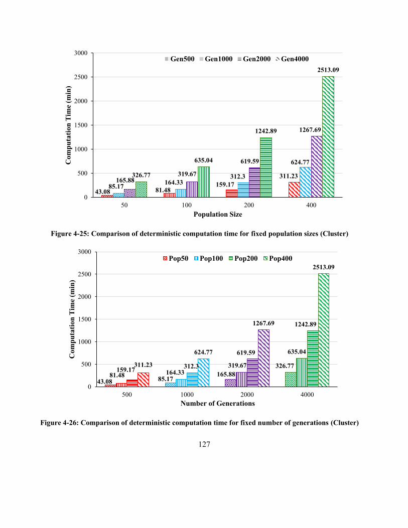
127

Figure 4-25: Comparison of deterministic computation time for fixed population sizes (Cluster)

Figure 4-26: Comparison of deterministic computation time for fixed number of generations (Cluster)

43.08 81.48159.17

311.23

85.17164.33

312.3

624.77

165.88319.67

619.59

1267.69

326.77

635.04

1242.89

2513.09

0

500

1000

1500

2000

2500

3000

50 100 200 400

Co

mp

uta

tio

n T

ime

(min

)

Population Size

Gen500 Gen1000 Gen2000 Gen4000

43.08 85.17165.88

326.77

81.48 164.33319.67

635.04

159.17312.3

619.59

1242.89

311.23

624.77

1267.69

2513.09

0

500

1000

1500

2000

2500

3000

500 1000 2000 4000

Com

pu

tati

on

Tim

e (m

in)


Pop50 Pop100 Pop200 Pop400

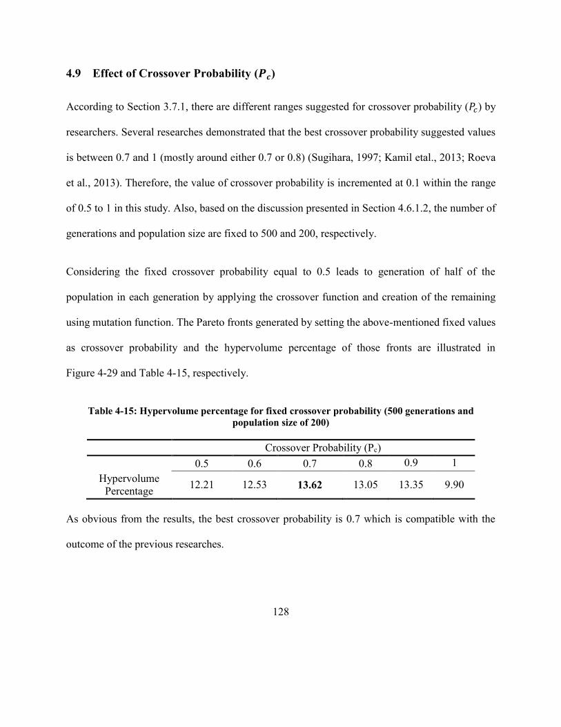
128

4.9 Effect of Crossover Probability (𝑷𝒄)

According to Section 3.7.1, there are different ranges suggested for crossover probability (𝑃𝑐) by

researchers. Several researches demonstrated that the best crossover probability suggested values

is between 0.7 and 1 (mostly around either 0.7 or 0.8) (Sugihara, 1997; Kamil etal., 2013; Roeva

et al., 2013). Therefore, the value of crossover probability is incremented at 0.1 within the range

of 0.5 to 1 in this study. Also, based on the discussion presented in Section 4.6.1.2, the number of

generations and population size are fixed to 500 and 200, respectively.

Considering the fixed crossover probability equal to 0.5 leads to generation of half of the

population in each generation by applying the crossover function and creation of the remaining

using mutation function. The Pareto fronts generated by setting the above-mentioned fixed values

as crossover probability and the hypervolume percentage of those fronts are illustrated in

Figure 4-29 and Table 4-15, respectively.

Table 4-15: Hypervolume percentage for fixed crossover probability (500 generations and

population size of 200)

Crossover Probability (Pc)

0.5 0.6 0.7 0.8 0.9 1

Hypervolume

Percentage 12.21 12.53 13.62 13.05 13.35 9.90

As obvious from the results, the best crossover probability is 0.7 which is compatible with the

outcome of the previous researches.

129

4.10 Effect of Number of Cores

In accordance with Section 3.7.2, the computation time which is needed to reach to the final

optimum results is calculated for different numbers of cores in order to investigate the ability of

parallel platform to improve the performance of the whole proposed framework. The performance

of the problem is measured using the number of cores set from 1 to 12. In order to omit the effect

of the uncertainty of the stochastic distribution of activities durations, all the durations are assumed

to be deterministic as given in Table 4-1. Table 4-17 and Figure 4-30 illustrate the computation

time needed to complete the simulation-based optimization based on 1000 generations and

population size of 100. The speedup achieved by increasing the number of cores is also illustrated

in Table 4-17. The speedup is calculated as S(1, n) = T1/Tn, where 𝑛, 𝑇1, and 𝑇𝑛 are the number of

the cores, computation time obtained by using one core, and parallel computation time obtained

by using 𝑛 cores, respectively (Yang et al., 2012). As shown in Table 4-17, using two and three

CPUs results in superliner speedup which means using these numbers of cores reduces the

computation time less than 1/2, and 1/3, respectively.

By increasing the number of cores more than three, the near linear speedup is achieved. For

instance, using 12 cores decreases the execution time of the proposed method to almost 1/8 of that

needed when using a single core. Also, there is less improvement in the computation time when

the number of cores exceed seven. These results show that the proposed method better uses the

computer capacity to reach to the optimal solutions by saving time.

130

Table 4-16: Improvement in the speed of running the integrated framework by the cluster while

fixing the population size

Population

Size

No. of

Generations Difference Percentage (%)

50

500 29.49

1000 28.23

2000 30.13

4000 30.97

100

500 25.83

1000 25.45

2000 27.80

4000 28.24

200

500 27.59

1000 28.77

2000 29.54

4000 29.08

400

500 28.92

1000 28.87

2000 26.45

4000 27.41

The parallel performance of the probabilistic simulation-based optimization procedure is also

investigated by assigning random distributions to the activities’ durations (Table 4-3). In this case,

the number of cores is also set from 1 to 12. For 100 generations, the size of population of 100 and

100 replications, the results are shown in Figure 4-31. The results indicate that there is a significant

improvement in the computation time by increasing the number of cores.

131

Figure 4-27: Time comparison between the performance of the Server machine and the cluster for the fixed population sizes

43.08

85.17

165.88

326.77

61.1

118.67

237.41

473.35

0

50

100

150

200

250

300

350

400

450

500

500 1000 2000 4000

Co

mp

uta

tio

n T

ime

(min

)


Cluster-Pop50 Server-Pop50

81.48164.33

319.67

635.04

109.85

220.44

442.74

884.94

0

100

200

300

400

500

600

700

800

900

1000

500 1000 2000 4000

Co

mp

uta

tio

n T

ime

(min

)



159.17312.3

619.59

1242.89

219.82

438.46

879.36

1752.51

0

200

400

600

800

1000

1200

1400

1600

1800

2000

500 1000 2000 4000

Co

mp

uta

tio

n T

ime

(min

)



311.23624.77

1267.69

2513.09

437.88

878.34

1723.51

3461.82

0

500

1000

1500

2000

2500

3000

3500

4000

500 1000 2000 4000

Co

mp

uta

tio

n T

ime

(min

)



132

Figure 4-28: Time comparison between the performance of the Server machine and the cluster for the fixed number of generations

43.08

81.48

159.17

311.23

61.1

109.85

219.82

437.88

0

50

100

150

200

250

300

350

400

450

500

50 100 200 400

Co

mp

uta

tio

n T

ime

(min

)

Population Size

Cluster-Gen500 Server-Gen500

85.17164.33

312.3

624.77

118.67

220.44

438.46

878.34

0

100

200

300

400

500

600

700

800

900

1000

50 100 200 400

Co

mp

uta

tio

n T

ime

(min

)

Population Size


165.88319.67

619.59

1267.69

237.41

442.74

879.36

1723.51

0

200

400

600

800

1000

1200

1400

1600

1800

2000

50 100 200 400

Co

mp

uta

tio

n T

ime

(min

)

Population Size


326.77635.04

1242.89

2513.09

473.35

884.94

1752.51

3461.82

0

500

1000

1500

2000

2500

3000

3500

4000

50 100 200 400

Co

mp

uta

tio

n T

ime

(min

)Population Size


133

Figure 4-29: Set of optimum solutions for different values as crossover probability

According to the number of replications that should be applied for the probabilistic mode, the

values of the computation time are much bigger than the deterministic mode; therefore, these

values are shown in hours instead of minutes in Table 4-18.

According to Section 3.6, the cluster has the ability to perform the proposed framework on multiple

nodes to take advantage of parallel execution of the model in more than one node in order to save

the computation time as much as possible. There are two types of nodes available in the McGill

University cluster with 12 cores and 16 cores. The core’s specifications are shown in Table 3-6. In

that table, phases 1 and 2 indicate the specification of nodes with 12 and 16 cores, respectively.

1400

1900

2400

2900

3400

3900

850 900 950 1000 1050 1100 1150 1200 1250 1300

CO

ST

(M

$)

DURATION (DAYS)

Pc = 0.5

Pc = 0.6

Pc = 0.7

Pc = 0.8

Pc = 0.9

Pc = 1

134

Table 4-17: Parallel computation time for deterministic mode (Server)

Number of Cores

1 2 3 4 5 6 7 8 9 10 11 12

Time (min) 1830 900 645 475 420 370 320 290 265 240 224 220

Speedup 1 2.03 2.84 3.85 4.36 4.95 5.72 6.31 6.91 7.63 8.17 8.32

Figure 4-30: Saving in Computation time by increasing the number of cores in deterministic mode

(Server)

Table 4-18: Parallel computation time for probabilistic mode (Server)

Number of Cores

1 2 3 4 5 6 7 8 9 10 11 12

Time (hrs.) 1015 398 245 151 121 102 87 77 69 61.02 58 50

Speedup 1 2.55 4.14 6.73 8.41 9.96 11.65 13.23 14.74 16.64 17.51 20.3

1830

900

645

475420

370320 290 265 240 224 220

0

200

400

600

800

1000

1200

1400

1600

1800

2000

1 2 3 4 5 6 7 8 9 10 11 12

Com

pu

tati

on

Tim

e (m

in.)

Number of Cores

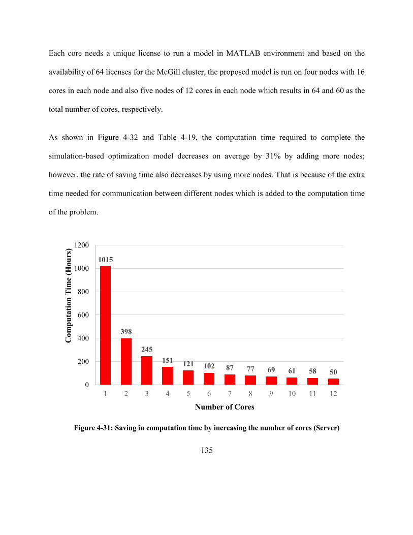
135

Each core needs a unique license to run a model in MATLAB environment and based on the

availability of 64 licenses for the McGill cluster, the proposed model is run on four nodes with 16

cores in each node and also five nodes of 12 cores in each node which results in 64 and 60 as the

total number of cores, respectively.

As shown in Figure 4-32 and Table 4-19, the computation time required to complete the

simulation-based optimization model decreases on average by 31% by adding more nodes;

however, the rate of saving time also decreases by using more nodes. That is because of the extra

time needed for communication between different nodes which is added to the computation time

of the problem.

Figure 4-31: Saving in computation time by increasing the number of cores (Server)

1015

398

245

151121 102 87 77 69 61 58 50

0

200

400

600

800

1000

1200

1 2 3 4 5 6 7 8 9 10 11 12

Com

pu

tati

on

Tim

e (H

ou

rs)

Number of Cores

136

Figure 4-32: Saving in computation time by increasing the number of nodes for 500 generations and

200 population size in deterministic mode (Cluster)

Table 4-19: Parallel computation time using multiple nodes (Cluster)

No. of Nodes Time (min)

Decrease Percentage 12 cores / Node 16 cores / Node

1 159 103 35.22

2 76 52 31.58

3 51 37 27.45

4 42 30 28.57

5 34 --- ---


This chapter investigated the procedure of developing different simulation models using

SimEvents along with the validation of the developed models by comparing the obtained results

of the simulation models with those obtained by Stroboscope in both deterministic and

probabilistic modes. It also discussed the integration of MATLAB optimization engine with the

159.17

75.88

51.0241.73

103.22

52.44

37.1429.78

0

20

40

60

80

100

120

140

160

180

1 2 3 4

Co

mp

uta

tio

n T

ime

(Min

)

Number of Nodes

12Cores

16Cores

137

developed SimEvents simulation model within a parallel environment. The proposed framework

is then validated by comparing the generated optimum solution with those obtained using another

type of GAs (fmGA). It discussed how changes in the various GA parameters affect the outcome

of the proposed system applying the sensitivity analysis on those parameters. Moreover, the

sensitivity analysis was performed by varying the number of cores in order to investigate the ability

of the parallel platform to improve the performance of the whole proposed framework. The

proposed parallel platform is implemented on two different systems: a server machine and the

cluster of McGill University.

The results of the comparison between the NSGA- and fmGA showed that the NSGA- resulted

in 4% better Pareto front compared with the results of fmGA. The outcomes of performing

sensitivity analysis on GA parameters such as the number of generations, size of population, and

crossover probability are used to tune the NSGA- based on the population size of 200, 500

generations, and crossover probability of 0.7. This GA configuration results in the most promising

optimal solutions considering the quality of solutions and computational efforts.

The parallel execution of the proposed framework on the server machine by using 12 cores results

in 8.32 and 20.3 times speedup compared with a single core for the deterministic and probabilistic

modes, respectively. Furthermore, running the parallel system on multiple nodes available at the

cluster improved the computation time by almost 31% using four nodes with 16 cores per node in

comparison with the same number of nodes and 12 cores per node. Moreover, the overall

comparison between the server machine and the cluster showed that both machines produce very

138

close optimum solutions in most of the cases; however, the cluster showed better performance

from the points of views of the quality of optimum solutions and computation time.

139

CHAPTER 5 SUMMARY, CONCLUSIONS AND FUTURE WORK

5.1 Summary of research

The research proposed the usage of NSGA- as the optimization engine integrated with SimEvents

DES to model different bridge construction processes. The parallel computing platform is then

applied to reduce the computation time necessary to deal with multiple objective functions and the

large search space.

Furthermore, it developed in detail the simulation modeling procedure using relatively new

simulation tool in the construction industry. It also elaborated on the needs, motivations and

benefits of performing the proposed framework within a parallel environment. Moreover, this

research proposed a comprehensive approach for investigating the effect of different GA

parameters on the performance of the proposed framework by performing sensitivity analysis. The

variation in the values of population size, number of generations, and crossover probability were

taken into account to identify the best configuration of GA parameters. The possible combinations

of GA parameters within the defined ranges and their impact on the system’s performance were

investigated. Furthermore, the sensitivity analysis is also performed by varying the number of

cores and nodes using two different machines including a server machine and the cluster of McGill

University.

The main advantages of the proposed framework are that it helps to find the best resource

combination among a large number of possible options by comparing sets of Pareto fronts, it

140

improves the computation time for both deterministic and stochastic simulation models using HPC,

and it suggests the most promising configuration of GA parameters in order to reach reliable and

optimum solutions.

5.2 Research contributions and conclusions

The conclusions of this research are as follows: (1) DES and multi-objective NSGA- are

integrated within a parallel environment to find the optimum solutions (i.e., the best resource

combinations) for a bridge construction method based on the objective functions’ values obtained

from the simulation. The optimal solutions obtained from the NSGA- optimization algoritm are

compared with those obtained from fmGA to validate the applicability of the proposed model. The

results showed that the NSGA- resulted in a Pareto front 4% better than that obtained from

fmGA; (2) 8.32 and 20.3 times speedup were achieved using master-salve parallel paradigm by

the server machine with 12 cores in deterministic and probabilistic modes, respectively; (3)

Furthermore, the NSGA- algorithm was tuned based on the best parameters which maximize its

performance by performing sensitivity analysis. The hypervolume indicator was used to compare

different Pareto fronts from the quality of optimum solutions point of view. The comparison of 32

sets of optimum solutions generate separately by both the server machine and the cluster results in

identification of the best settings of GA parameters as 500 generations, population size of 200 and

crossover probability of 0.7. In addition, performing the proposed framework on multiple nodes

using the cluster resulted in 31% saving on average in the computation time; (4) The overall

141

comparison between the performance of the server and the cluster showed 28.30% improvement

on average in computation time required by the cluster in comparison with the server.

5.3 Limitations and future work

Developing the simulation models in SimEvents as a relatively new simulation tool for

construction purposes has many difficulties and limitations since it is a graphical based simulation

tool which makes it difficult to either define common functions and concepts for construction

simulation models, and also to trace the simulation model. In addition, performing the proposed

framework on multiple nodes of the cluster has several limitations from the availability of the

nodes, license issues, and priority of submitted jobs by other users, which results in waiting in a

queue for long time in some cases.

The future research includes investigating the usage of different types of nodes on a cluster. Also,

according to the fact that by increasing the number of nodes the communication between the nodes

will increase as well, new solutions should be found to reduce the required communication

between nodes in order to improve the performance of the system from the computation time point

of view and to take full advantage of the capacity of multiple nodes for performing parallel jobs.

The hypervolume indicator can be used within the selection function as a selection criterion to

improve the performance of the optimization algorithm. Moreover, the sensitivity analysis of other

parameters of the GA, such as parameters within the creation and selection functions, is another

142

future work. In addition, the computational power of the proposed framework can be further

improved by testing other parallel computing approaches.

Finally, since the SimEvents is a relatively new emerging simulation tool for construction

purposes, improvements are expected in this tool to make it faster for simulating large-scale and

complex construction projects.

143

REFERENCES

Abendeh, R. E. (2006). Temperature Induced Deformations in Match-cast Segments and Their

Effects on Precast Segmental Bridges. Cuvillier Verlag.

AbouRizk, S. M., & Hajjar, D. (1998). A framework for applying simulation in construction.

Canadian journal of civil engineering, 25(3), 604-617.

AbouRizk, S. M., & Halpin, D. W. (1990). Probabilistic simulation studies for repetitive

construction processes. Journal of Construction Engineering and Management, 116(4),

575-594.

AbouRizk, S. M., Halpin, D. W., & Lutz, J. D. (1992). State of the Art in Construction Simulation.

Proceedings of the 1992 Winter Simulation Conference (pp. 1271-1277). Arlington: IEEE.

AbouRizk, S., & Shi, J. (1994). Automated construction-simulation optimization. Journal of

Construction Engineering and Management, 120(2), 374-385.

Abramson, D. A., Mills, G., & Perkins, S. (1993). Parallelisation of a genetic algorithm for the

computation of efficient train schedules. Proceedings of the 1993 Parallel Computing and

Transputers Conference, (pp. 139–149).

Abramson, D., & Abela, J. (1992). A parallel genetic algorithm for solving the school timetabling

problem. In Proceedings of the Fifteenth Australian Computer Science Conference (ACSC-

15), (pp. 1-11).

Accelerated Bridge Construction. (2014). In B. M. Tang, W. F. Chen, & L. Duan (Eds.), Bridge

Engineering Handbook: Construction and Maintenance. (pp. 175-206). Boca Raton: CRC

press.

Aissi, H., Bazgan, C., & Vanderpooten, D. (2009). Min–max and min–max regret versions of

combinatorial optimization problems: A survey. . European journal of operational research,

197(2), 427-438.

Al-Sudairi, A. A., Diekmann, J. E., Songer, A. D., & Brown, H. M. (1999). Simulation of

construction processes: traditional practices versus lean principles. In Seventh Conference

of the International Group for Lean Construction. 7, pp. 39-50. Berkeley, CA, USA:

University of California.

Anderson, E. J., & Ferris, M. C. (1994). A genetic algorithm for the assembly line balancing

problem. ORSA Journal on Computing, 6(2), 161-173.

Arditi, D., Elhassan, A., & Toklu, Y. (2002). Constructability Analysis in the Design Firm. Journal

of Construction Engineering and Management, 117-126.

Auger, A., Bader, J., Brockhoff, D., & Zitzler, E. (2009). Theory of the hypervolume indicator:

optimal μ-distributions and the choice of the reference point. Proceedings of the tenth ACM

144

SIGEVO workshop on Foundations of genetic algorithms (pp. 87-102). Orlando, Florida,

USA: ACM.

Barney, B. (2013). Introduction to Parallel Computing. Lawrence Livermore National Laboratory.

Belding, T. C. (1995). The distributed genetic algorithm revisited. arXiv preprint adap-

org/9504007. In Eschelman L., Ed., Proceedings of the Sixth International Conference on

Genetic Algorithms (pp. 114-121). San Francisco, CA: Morgan Kaufmann Publishers Inc.

Benaim, R. (2008). The Design of Prestressed Concrete Bridges. New York: Taylor & Francis.

Bianchini, R., & Brown, C. M. (1993). Parallel genetic algorithms on distributed-memory

architectures. Transputer Research and Applications 6 (pp. 67-82). Amsterdam: IOS Press.

Bradstreet, L. (2011). The Hypervolume Indicator for Multi-objective Optimization: Calculation

and Use. Perth: University of Western Australia.

Bridging by Segmental Box Girder. (2008). Retrieved from HupPages:

http://hazok.hubpages.com/hub/Bridging-by-Segmental-Box-Girder#

Bryant, R. E. (1977). Simulation of Packet Communication Architecture Computer Systems.

Cambridge, Massachusetts: Computer Science Laboratory, Massachusetts Institute of

Technology.

Buxton, J. N., & Laski, J. G. (1962). Control and simulation language. The Computer Journal,

5(3), 194-199.

Cantú-Paz, E. (1997). A Survey of Parallel Genetic Algorithms. Illinois Genetic Algorithms

Laboratory. Urbana: University of Illinois at Urbana-Champaign.

Cantú-Paz, E. (1998). A survey of parallel genetic algorithms. Calculateurs paralleles, reseaux et

systems repartis, 10(2), 141-171.

Cantú-Paz, E., & Goldberg, D. E. (2000). Efficient parallel genetic algorithms: theory and practice.

Computer Methods in Applied Mechanics and Engineering, 221-238.

Casseforme, N. (2013). Segmental Box Girder Forms. Retrieved from Bridge Formwork:

http://www.ninive.it/bridge-formwork/segmental-box-girder-forms/

Chandy, K. M., & Misra, J. (1979). Distributed simulation: A case study in design and verification

of distributed programs. . IEEE Transactions on Software Engineering, (pp. 440-452).

Chang, D. Y. (1986). RESQUE: A resource based simulation system for construction process

planning. Ann Arbor, Mich: PhD dissertation, University of Michigan.

Chang, D. Y., & Hoque, M. S. (1989). A Knowledge-based Simulation System for Construction

Process Planning. In Proceedings of the 6th International Symposium on Automation and

Robotics in Construction, (pp. 348-355).

Cheng, T. M., & Feng, C. W. (2003). An effective simulation mechanism for construction

operations. Automation in Construction, 12(3), 227-244.

Cheng, T. M., Feng, C. W., & Chen, Y. L. (2005). A hybrid mechanism for optimizing construction

simulation models. Automation in construction, 14(1), 85-98.

145

Cheng, T. M., Feng, C. W., & Hsu, M. Y. (2006). An integrated modeling mechanism for

optimizing the simulation model of the construction operation. Automation in construction,

15(3), 327-340.

Cheng, T. M., Wu, H. T., & Tseng, Y. W. (2000). Construction operation simulation tool–COST.

. In Symposium of 17th ISARC, (pp. 1143-1146). Taipei.

Clune, M. I., Mosterman, P. J., & Cassandras, C. G. (2006). Discrete event and hybrid system

simulation with simevents. Proceedings of 8th International Workshop on Discrete Event

Systems (pp. 386-387). Ann Arbor, Michigan, USA: IEEE.

Cohoon, J. P., Hegde, S. U., Martin, W. N., & Richards, D. (1987). Punctuated equilibria: a parallel

genetic algorithm. In Genetic algorithms and their applications: proceedings of the second

International Conference on Genetic Algorithms (pp. 148-154). Cambridge: The

Massachusetts Institute of Technology, MA. Hillsdale, NJ: L. Erlhaum Associates.

Cohoon, J. P., Martin, W. N., & Richards, D. S. (1991). A Multi-Population Genetic Algorithm

for Solving the K-Partition Problem on Hyper-Cubes. Proceedings of the Fourth

International Conference on Genetic Algorithms (pp. 244-248). San Mateo, CA: Morgan

Kaufmann.

Cohoon, J. P., Martin, W. N., & Richards, D. S. (1991). Genetic algorithms and punctuated

equilibria in VLSI. In H.-P. Schwefel, & R. Männer, Eds., Parallel Problem Solving from

Nature (pp. 134-144). Berlin, Heidelberg: Springer.

Continental Engineering Corporation. (2006). Full-span Precast and Launching Method. Retrieved

June 26, 2013, from http://www.continental-

engineering.com/english/page.php?cat_id=171&art_id=168

Dawood, N., & Shah, R. K. (2007). An Innovative Approach for Improvement of Communications

through Visual Schedule Model in Road Construction. 7th International Conference on

Construction Applications of Virtual Reality. University Park, Pennsylvania: Pennsylvania

State University.

Deb, K. (2001). Multi-objective optimization using evolutionary algorithms. Chichester: John

Wiley & Sons.

Deb, K. (2005). Muti-Objective Optimization. In E. Burke, & G. Kendall, Search Methodologies

Introductory Tutorials in Optimization and Decision Support Techniques (pp. 97-125).

United States of America: Springer Science-i-Business Media, LLC.

Deb, K., & Agrawal, R. B. (1995). Simulated binary crossover for continuous search space.

Complex Systems, 9(2), 115-148.

Deb, K., & Kumar, A. (1995). Real-coded Genetic Algorithms with Simulated Binary Crossover:

Studies on Multimodal and Multiobjective Problems. Complex Systems, 9, 431-454.

Deb, K., Anand, A., & Joshi, D. (2002). A computationally efficient evolutionary algorithm for

real-parameter optimization. Evolutionary computation, 10(4), 371-395.

146

Deb, K., Pratap, A., Agarwal, S., & Meyarivan, T. A. (2002). A fast and elitist multiobjective

genetic algorithm: NSGA-II. Evolutionary Computation, IEEE Transactions, 6(2), 182-

197.

Deep, K., & Thakur, M. (2007). A new crossover operator for real coded genetic algorithms.

Applied Mathematics and Computation, 188(1), 895-911.

Douglas, J. F., & Kosmas, M. K. (1989). Flexible polymer with excluded volume at an interacting

penetrable surface of variable dimension: a multiple-. Epsilon. perturbation theory.

Macromolecules, 22(5), 2412-2419.

El-Rayes, K., & Kandil, A. (2005). Time-Cost-Quality Trade-Off Analysis for Highway

Construction. Journal of Construction Engineering and Management, ASCE, 477-486.

Erdogan, J. E. (2009). Dubai LRT Viaducts Precast segmented span by span erection method.

Istanbul: FREYSSINET TURKEY.

Eshelman, L. J., & Schaffer, J. D. (1993). Real-Coded Genetic Algorithms and Interval-Schemata.

In L. Whitley, Foundations of genetic algorithms 2 (pp. 187-202). San Mateo, California:

Morgan Kaufmann.

Eshtehardian, E., Abbasnia, R., & Afshar, A. (2008). Optimization of uncertain construction time-

cost trade-off problem. Construction in Developing Countries (ICCIDC-I), (pp. 192-200).

Federal Highway Administration. (2013, January 22). Accelerated Bridge Construction. Retrieved

from http://www.fhwa.dot.gov/bridge/abc/index.cfm

Feng, C. W., Liu, L., & Burns, S. A. (2000). Stochastic construction time-cost trade-off analysis.

Journal of Computing in Civil Engineering, 14(2), 117-126.

Ferrada, X., Serpell, A., & Skibniewski, M. (2013). Selection of Construction Methods: A

Knowledge-Based Approach. The Scientific World Journal, 1-10.

Fleischer, M. (2003). The measure of Pareto optima applications to multi-objective metaheuristics.

Evolutionary multi-criterion optimization (pp. 519-533). Berlin Heidelberg: Springer.

Fogarty, T. C., & Huang, R. (1991). Implementing the genetic algorithm on transputer based

parallel processing systems. In Parallel Problem Solving from Nature (pp. 145-149).

Berlin, Heidelberg: Springer.

Fonseca, C. M., & Fleming, P. J. (1993). Genetic algorithms for multi-objective optimization:

Formulation, discussion and generalization. Proceedings of the Fifth International

Conference on Genetic Algorithms (pp. 416-423). California: Morgan Kauffman.

Fujimoto, R. M. (2001). Parallel simulation: parallel and distributed simulation systems. . In

Proceedings of the 33nd conference on winter simulation, IEEE Computer Society, (pp.

147-157).

Gaffney, J., Pearce, C., & Green, D. (2010). Binary versus real coding for genetic algorithms: A

false dichotomy? ANZIAM Journal, 51, C347-C359.

147

Gen, M., & Cheng, R. (2000). Genetic algorithms and engineering optimization. John Wiley &

Sons.

Gerwick, B. C. (1993). Construction of Prestressed Concrete Structures (2 nd Ed.). New York:

John Wiley & Sons.

Goldberg, D. (1989). Genetic algorithms in search, optimization and machine learning (Vol. 412).

Reading Menlo Park: Addison-wesley.

Goldberg, D. E. (1988). Genetic algorithms and machine learning. Machine learning, 3(2), 95-99.

Golden, L. (1998). Working time and the impact of policy institutions: Reforming the overtime

hours law and regulation. Review of Social Economy, 56(4), 522-541.

Gorges-Schleuter, M. (1989a). Asparagos: A population genetics approach to genetic algorithms.

In H. M. Voigt, H. Mühlenbein, & H. P. Schwefel, Evolution and Optimization, 89 (pp.

86-94). Berlin: Akademie-Verlag.

Gorges-Schleuter, M. (1989b). ASPARAGOS an asynchronous parallel genetic optimization

strategy. . In Proceedings of the 3rd International Conference on Genetic Algorithms (pp.

422-427). San Mateo, CA: Morgan Kaufmann Publishers Inc.

Grefenstette, J. J. (1981). Parallel Adaptive Algorithms for Function Optimization. Nashville, TN:

Computer Science Department, Vanderbilt University.

Grosso, P. B. (1985). Computer simulations of genetic adaptation: Parallel subcomponent

interaction in a multilocus model. Unpublished doctoral dissertation, The University of

Michigan.

Gruau, F. (1994). Neural Network Synthesis using Cellular Encoding and the Genetic Algorithm.

Villeurbanne, France: Doctoral dissertation, L’Universite Claude Bernard-Lyon I.

Guerra-Gómez, I., Tlelo-Cuautle, E., Reyes-Garcia, C. A., Reyes-Salgado, G., & de la Fraga, L.

G. (2009). Non-sorting genetic algorithm in the optimization of unity-gain cells. 6th

International Conference on Electrical Engineering, Computing Science and Automatic

Control, CCE, IEEE, (pp. 1-6).

Halpin, D. W. (1973). An investigation of the use of simulation networks for modeling

construction operations. Urbana-Champaign, Ill: PhD dissertation, Dept.of Civ. Engrg.,

University of Illinois.

Halpin, D. W. (1990). Micro-CYCLONE user’s manual. West Lafayette, Ind.: Dept. of Civ.

Engrg., Purdue University.

Halpin, D. W., & Riggs, L. S. (1992). Planning and Analysis of Construction Operations. New

York: John Wiley & Sons, Inc.

Halpin, D. W., & Woodhead, R. W. (1976). Design of construction and process operations. New

York: Wiley.

Hannon, J. J. (2007). Emerging technologies for construction delivery. Washington, D.C.:

Transportation Research Board, National Research Council, 2007.

148

Hauser, R., & Männer, R. (1994). Implementation of standard genetic algorithm on MIMD

machines. In Parallel Problem Solving from Nature, PPSN III (pp. 503-513). Berlin,

Heidelberg: Springer.

Hegazy, T., & Kassab, M. (2003). Resource optimization using combined simulation and genetic

algorithms. Journal of Construction Engineering and Management, ASCE, 129(6), 698-

705.

Hewson, N. R. (2003). Prestressed Concrete Bridges: Design and Construction. London: Thomas

Telford Ltd.

Hills, P. (1970). HOCUS: a new approach to simulation. In Software 70: proceedings of a

conference sponsored by Software world and held at the University of Sheffield, (p. 98).

Auerbach.

Hinterding, R. (1995). Gaussian mutation and self-adaption for numeric genetic algorithms. In

Evolutionary Computation, IEEE International Conference, 1, pp. 384-389.

Holland, J. (1959). A universal computer capable of executing an arbitrary number of sub-

programs simultaneously. In Papers presented at the December 1-3, 1959, eastern joint

IRE-AIEE-ACM computer conference, (pp. 108-113).

Holland, J. (1975). Adaptation in Natural and Artificial System. Ann Arbor, MI: University of

Michigan Press.

Holland, J. H. (1960). Iterative circuit computers. In Papers presented at the May 3-5, 1960,

western joint IRE-AIEE-ACM computer conference, (pp. 259-265).

Holt, A. S. (2008). Principles of construction safety. Oxford: Blackwell Science Ltd.

Horn, J., Nafploitis, N., & Goldberg, D. E. (1994). A niched Pareto genetic algorithm for multi-

objective optimization. Proceedings of the First IEEE Conference on Evolutionary

Computation (pp. 82-87). New Jersey: IEEE Service Center, Piscataway.

Iba, H., & Noman, N. (2012). New Frontier in Evolutionary Algorithms. London: Imperial College

Press.

Ioannou, P. G. (1989). UM-CYCLONE Discrete event simulation system reference manual. Ann

Arbor, Mich: Rep. No. UMCE-89-11, Dept. of Civil Engineering, Univ. of Michigan.

Janssen, A. J. (1995). Casting Box Girder Segments. The Aberdeen Group.

Jeannotte, K., & Chandra, A. (2005). Developing and implementing transportation management

plans for work zones. US Department of Transportation, Federal Highway Administration,

Office of Transportation Operations.

Jefferson, D. R. (1985). Virtual time. ACM Transactions on Programming Languages and Systems

(TOPLAS), 7(3), 404-425.

John R. Fowler, P. (2006). Accelerated Bridge Construction. Paper prepared for presentation at

the Bridges for the 21st Century session of the 2006 Annual Conference of the

Transportation Association of Canada. Charlottetown.

149

Kalk, A., & Douglas, S. A. (1980). INSIGHT: Interactive simulation of construction operations

using graphical techniques. Stanford, Calif: Tech. Rep. No. 238, Department of Civil

Engineering, Stanford University.

Kamil, K., Razali, N. M., & Teh, Y. Y. (2013). Sensitivity analysis of GA parameters for ECED

problem. In Power Engineering and Optimization Conference (PEOCO), 2013 IEEE 7th

International (pp. 256-260). Langkawi, Malaysia: IEEE.

Kandil, A., & El-Rayes, K. (2006). Parallel Genetic Algorithms for Optimizing Resource

Utilization in Large-Scale Construction Projects. Journal of Construction Engineering and

Management, ASCE, 132, 491-498.

Kandil, A., El-Rayes, K., & El-Anwar, O. (2010). Optimization research: Enhancing the

robustness of large-scale multiobjective optimization in construction. Journal of

construction engineering and management, ASCE, 136(1), 17-25.

Kim, I. Y., & De Weck, O. L. (2005). Adaptive weighted-sum method for bi-objective

optimization: Pareto front generation. Structural and multidisciplinary optimization, 29(2),

149-158.

Köksoy, O., & Yalcinoz, T. (2008). Robust Design using Pareto type optimization: A genetic

algorithm with arithmetic crossover. Computers & Industrial Engineering, 55(1), 208-218.

Kruisselbrink, J. (2011, March 17). Hypervolume Calculation [MATLAB Code].

Lacey, G., & Breen, J. (1969). Long Span Prestressed Concrete Bridges of Segmental Construction

State of the Art. Austin: Center for Highway Research the University of Texas.

Laumanns, M., Zitzler, E., & Thiele, L. (2000). A unified model for multi-objective evolutionary

algorithms with elitism. Proceedings of the 2000 Congress on Evolutionary Computation

(pp. 46-53). New Jersey: IEEE Service Center.

Lee, D.-E., Yi, C.-Y., Lim, T.-K., & Arditi, D. (2010). Integrated Simulation System for

Construction Operation and Project Scheduling. Journal of Computing in Civil

Engineering, ASCE, 557-569.

Li, X., & Kirley, M. (2002). The effects of varying population density in a fine-grained parallel

genetic algorithm. Proceedings of the 2002 Congress in Evolutionary Computation, IEEE,

2, pp. 1709-1714.

Li, X., Zhu, Y., & Zhang, Z. (2010). An LCA-based environmental impact assessment model for

construction processes. Building and Environment, 45(3), 766-775.

Lin, S. C., Goodman, E. D., & Punch III, W. F. (1997). Investigating parallel genetic algorithms

on job shop scheduling problems. Sixth International Conference on Evolutionary

Programming (pp. 383-393). Berlin: Springer-Verlag.

Lin, W. Y., Lee, W. Y., & Hong, T. P. (2003). Adapting crossover and mutation rates in genetic

algorithms. Journal of Information Sciences and Engineering, 19(5), 889-903.

150

Liu, L. (1991). COOPS: Construction object-oriented simulation system. Ann Arbor, Mich: PhD

dissertation, University of Michigan.

Liu, M., & Frangopol, D. M. (2005). Multiobjective maintenance planning optimization for

deteriorating bridges considering condition, safety, and life-cycle cost. Journal of

Structural Engineering, 131(5), 833-842.

Loannou, P. G., & Martinez, J. C. (2006). Stroboscope Quick Reference Manual. Ann Arbor,

Michigan: University of Michigan.

Lucko, G. (1999). Means and Methods Analysis of a Cast-In-Place Balanced Cantilever Segmental

Bridge: The Wilson Creek Bridge Case Study. Blacksburg, Virginia: Virginia Polytechnic

Institute and State University.

Maeda and Chun Wo Joint Venture. (1996). Match Casting Process. Retrieved from HUNG Hom

BYPASS: http://civcal.media.hku.hk/hunghom/precast_segments/match/_match3.htm

Mahoney, K. M., Porter, R. J., Taylor, D. R., Kulakowski, B. T., & Ullman, G. L. (2007). Design

of Construction Work Zones on High-Speed Highways. Highway and Facility Design,

NCHRP Report 581. Transportation Research Board of the National Academies,

Washington, D.C.: Transportation Research Board.

Manderick, B., & Spiessens, P. (1989). Fine-grained parallel genetic algorithms. In Proceedings

of the third international conference on Genetic algorithms (pp. 428-433). San Mateo, CA:

Morgan Kaufmann Publishers Inc.

Martinez, J. C. (1996). STROBOSCOPE: State and resource based simulation of construction

processes. Ann Arbor, Mich: PhD dissertation, University of Michigan.

Martinez, J. C. (1997). Structure of an advanced course in computer applications and simulation

in construction. Proc., 4th Congr. On Computing in Civ. Engrg., ASCE, (pp. 206-215).

Reston, Va.

Martinez, J. C. (1998). EarthMover—Simulation tool for earthwork planning. Proceedings of the

Winter Simulation Conference (pp. 1263-1271). Stockholm, Sweden: Royal Institute of

Technology.

Martinez, J. C., & Ioannou, P. G. (1994). General purpose simulation with stroboscope. . In

Proceedings of the 26th conference on winter simulation (pp. 1159-1166). Society for

Computer Simulation International.

Martinez, J. C., & Ioannou, P. G. (1999). General-purpose systems for effective construction

simulation. Journal of construction engineering and management, 125(4), 265-276.

Marzouk, M., & Moselhi, O. (2003). Object-oriented simulation model for earthmoving

operations. Journal of Construction Engineering and Management, 129(2), 173-181.

Marzouk, M., El-Dein, H., & El-Said, M. (2007). Application of Computer Simulation to

Construction of Incremental Launching Bridges. Journal of Civil Engineering and

Management, 13(1), 27-36.

151

Marzouk, M., Said, H., & El-Said, M. (2008). Special-Purpose Simulation Model for Balanced

Cantilever Bridges. Journal of Bridge Engineering, 13(2), 122-131.

MathWorks. (2013a). Multiobjective Genetic Algorithm Options. Retrieved from MathWorks,

Documentation Center: http://www.mathworks.com/help/gads/examples/multiobjective-

genetic-algorithm-options.html

MathWorks. (2013b). SimEvents User's Guide. The MathWorks, Inc.

Mathworks. (2014a). Profiling for Improving Performance. Retrieved from www.mathworks.com:

http://www.mathworks.com/help/matlab/matlab_prog/profiling-for-improving-

performance.html

MathWorks. (2014b). SimEvents, Model and simulate discrete-event systems. Retrieved from

MathWorks, Products & Services: http://www.mathworks.com/products/simevents/

MathWorks. (2014c). SIMULINK, Simulation and Model-Based Design. Retrieved from

MathWorks, Products & Services:

http://www.mathworks.com/products/simulink/?s_cid=wiki_simulink_2

MathWorks. (2014d). Simulink: A program for Simulating Dynamic Systems, User Guide. The

MathWorks, Inc.

MathWorks. (2014e). Multiobjective Genetic Algorithm Options. Retrieved from MathWorks,

Documentation Center: http://www.mathworks.com/help/gads/examples/multiobjective-

genetic-algorithm-options.html

Mawlana, M. (2013). Stochastic Simulation-based Optimization of Precast Box Girder Bridge

Construction Projects. Montreal: PhD Research Proposal at Concordia University.

Mawlana, M., & Hammad, A. (2013a). Framework for selecting a construction scenario for bridges

using simulation-based optimization. 4t Construction Specialty Conference, CSCE.

Montreal.

Mawlana, M., & Hammad, A. (2013b). Simulation-based Optimization of Precast Box Girder

Concrete Bridge Construction Using Full Span Launching Gantry. 4th Construction

Specialty Conference. Montreal.

Mawlana, M., Hammad, A., Doriani, A., & Setayeshgar, S. (2012). Discrete event simulation and

4D modelling for elevated highway reconstruction projects. In Proceedings of the XIVth

International Conference on Computing in Civil and Building Engineering. Moscow: State

University of Civil Engineering.

McCahill, D. F., & Bernold, L. E. (1993). Resource-oriented modeling and simulation in

construction. Journal of Construction Engineering and Management, 119(3), 590-606.

McGill-HPC. (2014, 08 04). Guillimin Hardware Information. Retrieved from

http://www.hpc.mcgill.ca: http://www.hpc.mcgill.ca/index.php/starthere/81-doc-

pages/215-guillimin-hardware

152

Michalewicz, Z. (1996). Genetic algorithms+ data structures= evolution programs (3rd Ed.). New

York: Springer-Verlag.

Mitchell, M. (1998). An introduction to genetic algorithms. MIT press.

Mohieldin, Y. A. (1989). Analysis of construction processes with nonstationary work task

durations. College Park: PhD diss., University of Maryland.

Moreton, A., & Janssen, H. (1995). Casting Box Girder Segments. The AberdeenGroup.

Mühlenbein, H. (1989a). Parallel genetic algorithms, population genetics, and combinatorial

optimization. In H. Voigt, H. Mühlenbein, & H. Schwefel, Evolution and Optimization ’89

(pp. 79-85). Berlin: Akademie-Verlag.

Mühlenbein, H. (1989b). Parallel genetic algorithms, population genetics and combinatorial

optimization. Proceedings of the Third International Conference on Genetic Algorithms

(pp. 416-421). San Mateo, CA: Morgan Kaufmann.

Mühlenbein, H., Schomisch, M., & Born, J. (1991). The parallel genetic algorithm as function

optimizer. Parallel computing, 17(6), 619-632.

Munawar, A., Wahib, M., Munetomo, M., & Akama, K. (2008). A survey: Genetic algorithms and

the fast evolving world of parallel computing. 10th IEEE International Conference in High

Performance Computing and Communications, HPCC'08, (pp. 897-902).

Nakayama, H., Yun, Y., & Yoon, M. (2009). Sequential Approximate Multiobjective Optimization

Using Computational Intelligence. Berlin: Springer-Verlag Berlin Heidelberg.

Naujoks, B., Beume, N., & Emmerich, M. (2005). Multi-objective Optimization Using S-metric

Selection: Application to Three-dimensional Solution Spaces. IEEE Congress on

Evolutionary Computation (CEC'2005) (p. 1282{1289). Edinburgh, Scotland: IEEE Press.

Nelson, B. L., Carson, J. S., & Banks, J. (2001). Discrete-Event System Simulation. Prentice hall.

Nelson, B., Nicol, D., Banks, J., & Carson II, J. (2013). Discrete-Event System Simulation (Fifth

Edition). Pearson Education.

Nicol, D., & Fujimoto, R. (1994). Parallel simulation today. Annals of Operations Research, 53(1),

249-285.

Nielsen. (2013, October 30). Conventional Bridge Construction vs. Accelerated Bridge

Construction. Retrieved from tallbridgeguy:

http://www.tallbridgeguy.com/2013/10/30/conventional-bridge-construction-vs-

accelerated-bridge-construction/

Nikakhtar, A., Wong, K. Y., Zarei, M. H., & Memari. (2011). Comparison of Two Simulation

Software for Modeling a Construction Process. In Computational Intelligence, Modelling

and Simulation (CIMSiM), 2011 Third International Conference, (pp. 200-205).

Niknam, T. (2010). A new fuzzy adaptive hybrid particle swarm optimization algorithm for non-

linear, non-smooth and non-convex economic dispatch problem. Applied Energy, 87(1),

327-339.

153

NIOSH. (2006). Fatality Assessment and Control Evaluation (FACE) Program. National Institute

for Occupational Saftey and Health (NIOSH).

NRS Bridge Construction Equipment. (2008). Full Span Method. Retrieved January 23, 2013,

from http://www.nrsas.com/equipments/fullspan.php

Odeh, A. M. (1992). Construction integrated planning and simulation model. Ann Arbor, Mich:

PhD dissertation, University of Michigan.

Oloufa, A. A. (1993, January). 1Modeling Operational Activities in Object-Oriented Simulation.

Journal of Computing in Civil Engineering, 7(1), 94-106.

Oloufa, A. A., & Ikeda, M. (1997). Library-based simulation modeling in construction. Proc., 4th

Congr. On Computing in Civ. Engrg., ASCE, (pp. 198-205). Reston, Va.

Ono, I., & Kobayashi, S. (1997). A Real Coded Genetic Algorithm for Function Optimization

Using Unimodal Normal Distributed Crossover. In Proceedings of the Seventh

International Conference on Genetic Algorithms (pp. 246-253). Morgan Kaufmann.

Orabi, W., El-Rayes, K., Senouci, A., & Al-Derham, H. (2009). Optimizing Postdisaster

Reconstruction Planning for Damaged Transportation Networks. Journal of Construction

Engineering and Management, 135(10), 1039-1048.

Orabi, W., Senouci, A. B., El-Rayes, K., & Al-Derham, H. (2010). Optimizing resource utilization

during the recovery of civil infrastructure systems. Journal of Management in Engineering,

26(4), 237-246.

Pan, N.-H., Chiu, T.-C., & Chen, K.-Y. (2008). Full-span Pre-cast Launching Method (FPLM)

analysis with Dynamic Simulation — Case studies of Taiwan High-Speed Rail (THSR)

Project. Automation in Construction, 17(5), 592–607.

Parmar, R. S., McClendon, R. W., & Potter, W. D. (1996). Farm machinery selection using

simulation and genetic algorithms. Transactions of the ASAE, 39(5), 1905-1909.

Paulson Jr, B. C., Chan, W. T., & Koo, C. C. (1987). Construction operations simulation by

microcomputer. Journal of construction engineering and management, 113(2), 302-314.

Perumalla, K. S. (2006). Parallel and distributed simulation: traditional techniques and recent

advances. Winter Simulation Conference (pp. 84-95). In Proceedings of the 38th

conference on winter simulation.

Pettey, C. B., Leuze, M. R., & Grefenstette, J. J. (1987). Parallel genetic algorithm. In Genetic

algorithms and their applications: proceedings of the second International Conference on

Genetic Algorithms (pp. 155-161). Cambridge: The Massachusetts Institute Institute of

Technology, MA. Hillsdale, NJ: L. Erlhaum Associates.

Pettey, C. C., & Leuze, M. R. (1989). A Theoretical Investigation of a Parallel Genetic Algorithm.

Proceedings of the Third International Conference on Genetic Algorithms (pp. 398-405).

San Mateo, CA): Morgan Kaufmann.

154

Purshouse, R. (2003). On the Evolutionary Optimization of Many Objectives. Doctoral

dissertation, University of Sheffield.

Reedy, J., & Lunzman, S. (2011). Model Based Design Accelerates Development of Mechanical

Locomotive Controls. Off-Highway Engineering, 19(2), 18-22.

Robinson, S. (2004). Simulation: The Practice of Model Development and Use. Wiley.

Roeva, O., Fidanova, S., & Paprzycki, M. (2013). Influence of the population size on the genetic

algorithm performance in case of cultivation process modelling. Federated Conference on

Computer Science and Information Systems (FedCSIS), IEEE, (pp. 371-376).

Rotolone, P. (2008). Gateway Bridge approaches– Match Casting of Box Segments. Queensland

Roads.

RSMeans Engineering Department. (2011). RS Means Heavy Construction Cost Data (25th ed.).

Norwell, MA: RS Means.

Sagert, P. (1995). Simulation of construction operations. Go¨teborg, Sweden: MS thesis, Chalmers

University of Technology.

Said, H., Marzouk, M., & El-Said, M. (2009). Application of computer simulation to bridge deck

construction: Case study. Automation in Construction, 18(4),, 18(4), 377-385.

Schwehm, M. (1992). Implementation of genetic algorithms on various interconnection networks.

Parallel computing and transputer applications (pp. 195-203). Amsterdam: IOS Press.

Serag, E., Oloufa, A., Malone, L., & Radwan, E. (2010). Model for quantifying the impact of

change orders on project cost for US roadwork construction. Journal of Construction


Shan, L. I., Gang, Y. A., Wen, Z., & Hong-liang, S. U. (2007). Fuzzy comprehensive assessment

of highway construction project impacts on environment. Journal of Chang'an University

(Natural Science Edition), 1(117).

Shi, J., & AbouRizk, S. M. (1997). Resource-based modeling for construction simulation. . Journal

of construction engineering and management, 123(1), 26-33.

Shimizu Corporation. (2013). Pakse Bridge (Laos). Retrieved from Shimz:

http://www.shimz.co.jp/english/theme/bridges/pakse.html

Sivanandam, S. N., & Deepa, S. N. (2008). Introduction to genetic algorithms. Verlag Berlin

Heidelberg: Springer.

Sivanandam, S. N., & Deepa, S. N. (2008). Genetic Algorithm Optimization Problems. Springer

Berlin Heidelberg.

Srinivas, M., & Patnaik, L. M. (1994). Genetic algorithms: A survey. Computer, 27(6), 17-26.

Srinivas, N., & Deb, K. (1994). Muiltiobjective optimization using nondominated sorting in

genetic algorithms. . Evolutionary computation, 2(3), 221-248.

155

Starkweather, T., Whitley, D., & Mathias, K. (1991). Optimization using distributed genetic

algorithms. In S. H.-P., & M. R., Parallel Problem Solving from Nature (pp. 176-185).

Berlin Heidelberg: Springer.

Sugihara, K. (1997). Measures for performance evaluation of genetic algorithms. In Proc. of the

3rd. joint Conference on Information Sciences, (pp. 172-175).

Tamaki, H., & Nishikawa, Y. (1992). A paralleled genetic algorithm based on a neighborhood

model and its application to the jobshop scheduling. Parallel problem solving from nature

(pp. 573-582). Amsterdam: Elsevier Science.

Tanese, R. (1987). Parallel genetic algorithm for a hypercube. . In Genetic algorithms and their

applications: proceedings of the second International Conference on Genetic Algorithms

(pp. 177-183). Cambridge: The Massachusetts Institute of Technology, Cambridge, MA.

Hillsdale, NJ: L. Erlhaum Associates.

Tanese, R. (1989). Distributed genetic algorithms. In Proceedings of the third international

conference on Genetic algorithms (pp. 434-439). San Mateo, CA: Morgan Kaufmann

Publishers Inc.

Tang, B. M. (2014). Accelerated Bridge Construction. In B. Launchinh, B. Skidding, & P. M.

Transporters, Bridge Engineering Handbook: Construction and Maintenance (pp. 175-

206). Taylor & Francis Group, LLC.

Tang, L., Jing, X., Sun, S., & Xiao, X. (2011). An adaptive location algorithm for flexible indoor

environment. Cross Strait Quad-Regional Radio Science and Wireless Technology

Conference (CSQRWC), IEEE, 2, pp. 1050-1053.

Tennessee, T. U. (2014). HPC Glossary. Retrieved from NICS: The Natinal Institute for

Computational Sciences: https://www.nics.tennessee.edu/hpc-glossary

Thomas, H. R., Maloney, W. F., Horner, R. M., Smith, G. R., Handa, V. K., & Sanders, S. R.

(1990). Modeling construction labor productivity. Journal of Construction Engineering and

Management, 116(4), 705-726.

Tocher, K. D., & Owen, D. G. (1960). The automatic programming of simulations. Proc., IFORS

Conference, (pp. 50-67). IFORS, Aix-en-Provence.

Touran, A. (1990). Integration of Simulation with Expert Systems. Journal of Construction


Tsutsui, S., Yamamura, M., & Higuchi, T. (1999). Multi-parent recombination with simplex

crossover in real coded genetic algorithms. In Proceedings of the genetic and evolutionary

computation conference, 1, pp. 657-664.

Ugwu, O. O., & Tah, J. H. (1998). Towards optimising construction-method selection strategies

using genetic algorithms. Engineering Applications of Artificial Intelligence, 11(4), 567-

577.

156

Valigura, K., Foltin, M., & Blaho, M. (2009). Transport System Realization in SimEvents Tools.

Technical Computing Prague.

Venkataraman, P. (2009). Applied optimization with MATLAB programming. Hoboken, New

Jersey: John Wiley & Sons, Inc.

Vidalis, S. M., & Najafi, F. T. (2002). Cost and time overruns in highway construction. In 4th

Transportation Speciality Conference (pp. 5-8). Montreal: Canadian Society for Civil

Engineering.

VSL International Ltd. (2013). Bridge Construction Technology. Retrieved January 23, 2013, from

http://www.vsl.com/index.php?option=com_content&view=article&id=82&Itemid=188

Wainer, G. A. (2009). Discrete-Event Modeling and Simulation. A Practitioner's Approach. Boca

Raton: CRC Press.

Wakefield, R. R., & Sears, G. A. (1997). Petri nets for simulation and modeling of construction

systems. Journal of Construction Engineering and Management, 123(2), 105-112.

WisDOT Bridge Manual. (2013). Chapter 7-Accelerated Bridge Construction. Wisconsin

Department.

Wu, C. H., Hsieh, T. Y., & Cheng, W. L. (2005). Statistical analysis of causes for design change

in highway construction on Taiwan. International journal of project management, 23(7),

554-563.

Wu, H. J., Chang, Y. H., Hwang, M. S., & Lin, I. C. (2009). Flexible RFID location system based

on artificial neural networks for medical care facilities. Taichung, Taiwan: Department of

Management Information Systems, National Chung Hsing University.

Wu, Z. Y., Wang, Q., Butala, S., Mi, T., & Song, Y. (2012). Darwin Optimization Framework

User Manual. . Incorporated, Watertown, CT, 6795: Bentley Systems.

Yang, I. T., Hsieh, Y. M., & Kung, L. O. (2012). Parallel computing platform for multiobjective

simulation optimization of bridge maintenance planning. Journal of Construction


Yifu, C. Y. (2005). Study on the Application of the IAHP Method in Environmental Influence

Comprehensive Evaluation in Highway Construction. Industrial Safety and Dust Control,

11(014).

Yuan, W. N., & Ren, Z. (1999). Integrated assessment of highway environmental impact. Journal

of Xi'an Highway University, 19(50).

Zhang, C., & Hammad, A. (2005). Spatio-temporal issues in infrastructure lifecycle management

systems. In Proceedings of 1st CSCE Specialty Conference on Infrastructure Technologies,

Management and Policy (pp. FR-131--1-FR-131--10). Toronto: Canadian Society for Civil

Engineering (CSCE).

Zitzler, E. (1999). Evolutionary Algorithms for Multiobjective Optimization: Methods and

Applications. Zurich, Switzerland: Swiss Federal Institute of Technology (ETH).

157

Zitzler, E., & Thiele, L. (1999). Multiobjective evolutionary algorithms: a comparative case study

and the strength Pareto approach. IEEE Transactions on Evolutionary Computation, 3(4),

257-271.

Zitzler, E., Thiele, L., Laumanns, M., Fonseca, C. M., & Da Fonseca, V. G. (2003). Performance

assessment of multiobjective optimizers: An analysis and review. IEEE Transactions

Evolutionary Computation, 7(2), 117-132.

158

APPENDICES

159

Appendix A – MATLAB code of deterministic simulation (DES)

% Functions to be minimized

function y = ObjectivFunctions_Det(x)

%% Initial Setting

% OP = Overtime policy % Rep= Number of replications

OP=[1 1 1 8 5 1 1.039 1.111 9 5 1 1.096 1.200 10 5 1 1.231 1.273 11 5 1 1.311 1.333 12 5 1 1.039 1.167 8 6 1 1.081 1.259 9 6 1 1.143 1.333 10 6 1 1.269 1.394 11 6 1 1.356 1.444 12 6 1 1.127 1.286 8 7 1 1.194 1.365 9 7 1 1.270 1.429 10 7 1 1.379 1.481 11 7 1 1.455 1.524 12 7];

Rep=1; TruckDriverHrCost=50; YardCraneDriverHrCost=100; OnsiteCraneDriverHrCost=100; TrolleyDriverHrCost=100; GantryDriverHrCost=200; OtherDailyCost=500; YardCraneHrCost=50; DelTruckHrCost=50; GantryInitCost=9000; GantryHrCost=500; TrolleyInitCost=900; TrolleyHrCost=150; OnsiteCraneInitCost=900; OnsiteCraneHrCost=150; CageInitCost=500; CageHrCost=10; InnerMouldInitCost=1000; InnerMouldHrCost=10; OuterMouldInitCost=1000; OuterMouldHrCost=10; PrepCrewInitCost=200; PrepCrewHrCost=200;

160

PrestressCrewInitCost=200; PrestressCrewHrCost=200; SteelCrewInitCost=200; SteelCrewHrCost=200; CastCrewInitCost=200; CastCrewHrCost=200; StorageHourlyCost=10; NPrecastSpans=4; NGantry=1; NOnsiteCrane=1; NYardCrane=1; NYardCrane1=1; NOnsiteTrolley=1; CureMethodDuration=[600 1200]; CureMethodCost=[200 0]; NTrailer=x(1); PrecastYardDistance=x(2); NRebarCageMold=x(3); NInnerMold=x(4); NOuterMold=x(5); NPreperationCrew=x(6); NStressingCrew=x(7); NSteelCrew=x(8); NCastingCrew=x(9); CureMethodD=x(10); F=x(11); NStorageCapacity=x(12); StorageTime=x(13);

% Parallel execution of simulation model

parfor i = 1:Rep; % Input variables from MOGA to Discrete Event Simulation (DES) set_param('CastingOperation_withoptimization_final_Deterministic_BMDet/Traile

r Queue/Time-Based Function-Call Generator2','NumberOfEventsPerPeriod',

num2str(NTrailer)); set_param('CastingOperation_withoptimization_final_Deterministic_BMDet/Rebar-

Mold Queue/Time-Based Function-Call Generator1','NumberOfEventsPerPeriod',

num2str(NRebarCageMold)); set_param('CastingOperation_withoptimization_final_Deterministic_BMDet/InnerM

old Queue/Time-Based Function-Call Generator','NumberOfEventsPerPeriod',

num2str(NInnerMold)); set_param('CastingOperation_withoptimization_final_Deterministic_BMDet/Outer_

Mold Queue/Time-Based Function-Call Generator','NumberOfEventsPerPeriod',

num2str(NOuterMold)); set_param('CastingOperation_withoptimization_final_Deterministic_BMDet/Prep_C

rew Queue/Time-Based Function-Call Generator2','NumberOfEventsPerPeriod',

num2str(NPreperationCrew)); set_param('CastingOperation_withoptimization_final_Deterministic_BMDet/Stress

ing_Crew Queue/Time-Based Function-Call Generator2','NumberOfEventsPerPeriod',

num2str(NStressingCrew));

161

set_param('CastingOperation_withoptimization_final_Deterministic_BMDet/Steel_

Crew Queue/Time-Based Function-Call Generator2','NumberOfEventsPerPeriod',

num2str(NSteelCrew)); set_param('CastingOperation_withoptimization_final_Deterministic_BMDet/Cast_C

rew Queue/Time-Based Function-Call Generator2','NumberOfEventsPerPeriod',

num2str(NCastingCrew)); set_param('CastingOperation_withoptimization_final_Deterministic_BMDet/Storag

e-Cap Queue/Time-Based Function-Call Generator','NumberOfEventsPerPeriod',

num2str(NStorageCapacity*5)); set_param('CastingOperation_withoptimization_final_Deterministic_BMDet/Bottom

Slab-Web/BottomSlab_Web','ServiceTime', num2str(1673*OP(F,2))); set_param('CastingOperation_withoptimization_final_Deterministic_BMDet/Inner_

Mold/Inner_Mold','ServiceTime', num2str(300*OP(F,2))); set_param('CastingOperation_withoptimization_final_Deterministic_BMDet/TopSla

b/TopSlab','ServiceTime', num2str(1979*OP(F,2))); set_param('CastingOperation_withoptimization_final_Deterministic_BMDet/LiftTo

Mold/LiftToMold','ServiceTime', num2str(45*OP(F,2))); set_param('CastingOperation_withoptimization_final_Deterministic_BMDet/Cast_S

pan/Cast_Span','ServiceTime', num2str(1544*OP(F,2))); set_param('CastingOperation_withoptimization_final_Deterministic_BMDet/Span_C

uring/Span_Curing','ServiceTime', num2str(CureMethodDuration(CureMethodD))); set_param('CastingOperation_withoptimization_final_Deterministic_BMDet/Remove

InnerMol/RemoveInnerMol','ServiceTime', num2str(255*OP(F,2))); set_param('CastingOperation_withoptimization_final_Deterministic_BMDet/Postte

nsion_1st/Posttension_1st','ServiceTime', num2str(240*OP(F,2))); set_param('CastingOperation_withoptimization_final_Deterministic_BMDet/LiftTo

Storage/LiftToStorage','ServiceTime', num2str(60*OP(F,2))); set_param('CastingOperation_withoptimization_final_Deterministic_BMDet/Postte

nsion_2nd/Posttension_2nd','ServiceTime', num2str(240*OP(F,2))); set_param('CastingOperation_withoptimization_final_Deterministic_BMDet/Storag

e_Time/Storage_Time','ServiceTime', num2str(StorageTime*60)); set_param('CastingOperation_withoptimization_final_Deterministic_BMDet/Traile

r_Loading/Trailer_Loading','ServiceTime', num2str(60*OP(F,2))); set_param('CastingOperation_withoptimization_final_Deterministic_BMDet/Traile

r_Haul/Trailer_Haul','ServiceTime', num2str(PrecastYardDistance*10*0.67)); set_param('CastingOperation_withoptimization_final_Deterministic_BMDet/Trolle

y_Loading/Trolley_Loading','ServiceTime', num2str(60*OP(F,2))); set_param('CastingOperation_withoptimization_final_Deterministic_BMDet/Trolle

y_Travel and Trailer_Return/Trailer_Return','ServiceTime',

num2str(PrecastYardDistance*10*0.67)); set_param('CastingOperation_withoptimization_final_Deterministic_BMDet/Reposi

tion/Reposition','ServiceTime', num2str(240*OP(F,2))); set_param('CastingOperation_withoptimization_final_Deterministic_BMDet/Pickup

_Span/Pickup_Span','ServiceTime', num2str(60*OP(F,2))); set_param('CastingOperation_withoptimization_final_Deterministic_BMDet/Trolle

y_Return and Erect_Span/Erect_Span','ServiceTime', num2str(240*OP(F,2))); set_param('CastingOperation_withoptimization_final_Deterministic_BMDet/Prepar

e_Bearing/Prepare_Bearing','ServiceTime', num2str(240*OP(F,2))); set_param('CastingOperation_withoptimization_final_Deterministic_BMDet/Load_T

ransfer/Load_Transfer','ServiceTime', num2str(60*OP(F,2))); % Run DES

162

simOut{i} =

sim('CastingOperation_withoptimization_final_Deterministic_BMDet','SaveOutput

','on','OutputSaveName','tout','OutputSaveName','BottomSlab_Web','OutputSaveN

ame','BottomSlab_Web1'...

,'OutputSaveName','Inner_Mold','OutputSaveName','TopSlab','OutputSaveName','L

iftToMold','OutputSaveName','Cast_Span','OutputSaveName','Span_Curing'...

,'OutputSaveName','RemoveInnerMol','OutputSaveName','Posttension_1st','Output

SaveName','LiftToStorage','OutputSaveName','Posttension_2nd','OutputSaveName'

,'Storage_Time'...

,'OutputSaveName','Trailer_Loading','OutputSaveName','Trailer_Haul','OutputSa

veName','Trolley_Loading','OutputSaveName','Trailer_Return','OutputSaveName',

'Trolley_Travel'...

,'OutputSaveName','Reposition','OutputSaveName','Pickup_Span','OutputSaveName

','Trolley_Return','OutputSaveName','Erect_Span'...

,'OutputSaveName','Prepare_Bearing','OutputSaveName','Load_Transfer');

end % Get outputs from DES to MOGA output = cell(Rep,23);

for i=1:Rep output{i,1}=simOut{i}.get('tout'); output{i,2}= simOut{i}.get('BottomSlab_Web1'); output{i,3}= simOut{i}.get('BottomSlab_Web'); output{i,4}= simOut{i}.get('Inner_Mold'); output{i,5}= simOut{i}.get('TopSlab'); output{i,6}= simOut{i}.get('LiftToMold'); output{i,7}= simOut{i}.get('Cast_Span'); output{i,8}= simOut{i}.get('Span_Curing'); output{i,9}= simOut{i}.get('RemoveInnerMol'); output{i,10}= simOut{i}.get('Posttension_1st'); output{i,11}= simOut{i}.get('LiftToStorage'); output{i,12}= simOut{i}.get('Posttension_2nd'); output{i,13}= simOut{i}.get('Storage_Time'); output{i,14}= simOut{i}.get('Trailer_Loading'); output{i,15}= simOut{i}.get('Trailer_Haul'); output{i,16}= simOut{i}.get('Trolley_Loading'); output{i,17}= simOut{i}.get('Trailer_Return'); output{i,18}= simOut{i}.get('Trolley_Travel'); output{i,19}= simOut{i}.get('Reposition'); output{i,20}= simOut{i}.get('Pickup_Span'); output{i,21}= simOut{i}.get('Trolley_Return'); output{i,22}= simOut{i}.get('Erect_Span'); output{i,23}= simOut{i}.get('Prepare_Bearing'); % First objective function (total duration of the process) calculations Nt=(cell2mat(output(i,1)));

TWorkingDays=round(Nt/(60*OP(F,4))+0.49); TProjectDuration=TWorkingDays+ floor(TWorkingDays/OP(F,5))*(7-OP(F,5));

% Second objective function (total cost of the process) calculations

163

TSetupCost=

2*(NCastingCrew*CastCrewInitCost*OP(F,1)+NRebarCageMold*CageInitCost+NInnerMo

ld*InnerMouldInitCost+NOuterMold*OuterMouldInitCost...

+NPreperationCrew*PrepCrewInitCost*OP(F,1)+NStressingCrew*PrestressCrewInitCo

st*OP(F,1)+NSteelCrew*SteelCrewInitCost*OP(F,1)+NGantry*GantryInitCost+NOnsit

eTrolley*TrolleyInitCost+NOnsiteCrane*OnsiteCraneInitCost);

TIndirectCost=TProjectDuration*OtherDailyCost; TCuringCost=CureMethodCost(CureMethodD)*NPrecastSpans;

TDirectCost=(NCastingCrew*CastCrewHrCost*OP(F,1)*OP(F,3)*(output{i,7}.time(50

1)+((output{i,7}.time(2))-(output{i,6}.time(2)))-

(output{i,7}.time(2)))+(NRebarCageMold*CageHrCost*(output{i,6}.time(501)-

output{i,2}.time(2))))+(NInnerMold*InnerMouldHrCost*(output{i,9}.time(501)-

(output{i,4}.time(2)-(output{i,4}.time(2)-output{i,3}.time(2)))))... +(NOuterMold*OuterMouldHrCost*(output{i,11}.time(501)-

(output{i,6}.time(2)-(output{i,6}.time(2)-output{i,5}.time(2)))))...

+(NPreperationCrew*PrepCrewHrCost*OP(F,1)*OP(F,3)*(output{i,9}.time(501)-


+(NStressingCrew*PrestressCrewHrCost*OP(F,1)*OP(F,3)*(output{i,12}.time(501)-

(output{i,10}.time(2)-(output{i,10}.time(2)-output{i,9}.time(2)))))... +(NSteelCrew*SteelCrewHrCost*OP(F,1)*OP(F,3)*(output{i,5}.time(501)-

output{i,2}.time(2)))... +(NTrailer*DelTruckHrCost*(output{i,17}.time(501)-(output{i,14}.time(2)-

(output{i,14}.time(2)-output{i,13}.time(2)))))...

+(NYardCrane*YardCraneHrCost*(output{i,14}.time(501)+((output{i,14}.time(2))-

(output{i,13}.time(2)))-(output{i,14}.time(2))))... +(NYardCrane1*YardCraneHrCost*(output{i,11}.time(501)-

(output{i,6}.time(2)-(output{i,6}.time(2)-output{i,5}.time(2)))))... +(NGantry*GantryHrCost*(output{i,22}.time(501)-(output{i,19}.time(2)-

(output{i,19}.time(2)-output{i,18}.time(2)))))... +(NOnsiteTrolley*TrolleyHrCost*(output{i,21}.time(501)-


+(NOnsiteCrane*OnsiteCraneHrCost*(output{i,16}.time(501)+((output{i,16}.time(

2))-(output{i,15}.time(2)))-(output{i,16}.time(2))))... +(NTrailer*TruckDriverHrCost*OP(F,1)*OP(F,3)*(output{i,17}.time(501)-


+(NYardCrane*YardCraneDriverHrCost*OP(F,1)*OP(F,3)*(output{i,14}.time(501)+((

output{i,14}.time(2))-(output{i,13}.time(2)))-(output{i,14}.time(2))))...

+(NYardCrane1*YardCraneDriverHrCost*OP(F,1)*OP(F,3)*(output{i,11}.time(501)-


+(NGantry*GantryDriverHrCost*OP(F,1)*OP(F,3)*(output{i,22}.time(501)-


+(NOnsiteTrolley*TrolleyDriverHrCost*OP(F,1)*OP(F,3)*(output{i,21}.time(501)-


+(NOnsiteCrane*OnsiteCraneDriverHrCost*OP(F,1)*OP(F,3)*(output{i,16}.time(501

)+((output{i,16}.time(2))-(output{i,15}.time(2)))-(output{i,16}.time(2))))...

+(NStorageCapacity*5*(StorageHourlyCost/(PrecastYardDistance*10))*(output{i,1

3}.time(501)+((output{i,13}.time(2))-(output{i,12}.time(2)))-

(output{i,13}.time(2))));

164

TotalCost=round(((TSetupCost+TCuringCost+TDirectCost+TIndirectCost)/1000000)+

0.49); end

% Mean values of objective functions y(1)=mean(TProjectDuration); y(2)=mean(TotalCost);

Appendix B – MATLAB code of probabilistic simulation (DES)

% Functions to be minimized

function y = ObjectivFunctions_Prob(x)

%% Initial Setting

% OP = Overtime policy % Rep= Number of replications

OP=[1 1 1 8 5 1 1.039 1.111 9 5 1 1.096 1.200 10 5 1 1.231 1.273 11 5 1 1.311 1.333 12 5 1 1.039 1.167 8 6 1 1.081 1.259 9 6 1 1.143 1.333 10 6 1 1.269 1.394 11 6 1 1.356 1.444 12 6 1 1.127 1.286 8 7 1 1.194 1.365 9 7 1 1.270 1.429 10 7 1 1.379 1.481 11 7 1 1.455 1.524 12 7];

Rep=100; TruckDriverHrCost=50; YardCraneDriverHrCost=100; OnsiteCraneDriverHrCost=100; TrolleyDriverHrCost=100; GantryDriverHrCost=200; OtherDailyCost=500; YardCraneHrCost=50; DelTruckHrCost=50; GantryInitCost=9000; GantryHrCost=500; TrolleyInitCost=900; TrolleyHrCost=150; OnsiteCraneInitCost=900;

165

OnsiteCraneHrCost=150; CageInitCost=500; CageHrCost=10; InnerMouldInitCost=1000; InnerMouldHrCost=10; OuterMouldInitCost=1000; OuterMouldHrCost=10; PrepCrewInitCost=200; PrepCrewHrCost=200; PrestressCrewInitCost=200; PrestressCrewHrCost=200; SteelCrewInitCost=200; SteelCrewHrCost=200; CastCrewInitCost=200; CastCrewHrCost=200; StorageHourlyCost=10; NPrecastSpans=4; NGantry=1; NOnsiteCrane=1; NYardCrane=1; NYardCrane1=1; NOnsiteTrolley=1; CureMethodDuration=[600 1200]; CureMethodCost=[200 0]; NTrailer=x(1); PrecastYardDistance=x(2); NRebarCageMold=x(3); NInnerMold=x(4); NOuterMold=x(5); NPreperationCrew=x(6); NStressingCrew=x(7); NSteelCrew=x(8); NCastingCrew=x(9); CureMethodD=x(10); F=x(11); NStorageCapacity=x(12); StorageTime=x(13);

% Parallel execution of simulation model

parfor i = 1:Rep; seed = mod(floor((i/Rep) * now * 8640000),2^31-1);

se_randomizeseeds('CastingOperation_withoptimization_final_Probabilistic_BMPr

ob','GlobalSeed',seed); set_param('CastingOperation_withoptimization_final_Probabilistic_BMProb/Trail

er Queue/Time-Based Function-Call Generator2','NumberOfEventsPerPeriod',

num2str(NTrailer)); set_param('CastingOperation_withoptimization_final_Probabilistic_BMProb/Trail

er_Haul/Subsystem/Atomic Subsystem/Bias','Bias',

num2str((0.67)*10*PrecastYardDistance));

166

set_param('CastingOperation_withoptimization_final_Probabilistic_BMProb/Troll

ey_Travel and Trailer_Return/Subsystem1/Atomic Subsystem/Bias','Bias',

num2str((0.67)*10*PrecastYardDistance)); set_param('CastingOperation_withoptimization_final_Probabilistic_BMProb/Rebar

-Mold Queue/Time-Based Function-Call Generator1','NumberOfEventsPerPeriod',

num2str(NRebarCageMold)); set_param('CastingOperation_withoptimization_final_Probabilistic_BMProb/Inner

Mold Queue/Time-Based Function-Call Generator','NumberOfEventsPerPeriod',

num2str(NInnerMold)); set_param('CastingOperation_withoptimization_final_Probabilistic_BMProb/Outer

_Mold Queue/Time-Based Function-Call Generator','NumberOfEventsPerPeriod',

num2str(NOuterMold)); set_param('CastingOperation_withoptimization_final_Probabilistic_BMProb/Prep_


num2str(NPreperationCrew)); set_param('CastingOperation_withoptimization_final_Probabilistic_BMProb/Stres

sing_Crew Queue/Time-Based Function-Call

Generator2','NumberOfEventsPerPeriod', num2str(NStressingCrew)); set_param('CastingOperation_withoptimization_final_Probabilistic_BMProb/Steel

_Crew Queue/Time-Based Function-Call Generator2','NumberOfEventsPerPeriod',

num2str(NSteelCrew)); set_param('CastingOperation_withoptimization_final_Probabilistic_BMProb/Cast_


num2str(NCastingCrew)); set_param('CastingOperation_withoptimization_final_Probabilistic_BMProb/Stora

ge-Cap Queue/Time-Based Function-Call Generator','NumberOfEventsPerPeriod',

num2str(5*NStorageCapacity)); set_param('CastingOperation_withoptimization_final_Probabilistic_BMProb/Stora

ge_Time/Storage_Time','ServiceTime', num2str(StorageTime)); set_param('CastingOperation_withoptimization_final_Probabilistic_BMProb/Span_

Curing/Span_Curing','ServiceTime', num2str(CureMethodDuration(CureMethodD))); set_param('CastingOperation_withoptimization_final_Probabilistic_BMProb/Botto

mSlab-Web/Gain','Gain', num2str(OP(F,2))); set_param('CastingOperation_withoptimization_final_Probabilistic_BMProb/Inner

_Mold/Gain','Gain', num2str(OP(F,2))); set_param('CastingOperation_withoptimization_final_Probabilistic_BMProb/TopSl

ab/Gain','Gain', num2str(OP(F,2))); set_param('CastingOperation_withoptimization_final_Probabilistic_BMProb/LiftT

oMold/Gain','Gain', num2str(OP(F,2))); set_param('CastingOperation_withoptimization_final_Probabilistic_BMProb/Cast_

Span/Gain','Gain', num2str(OP(F,2))); set_param('CastingOperation_withoptimization_final_Probabilistic_BMProb/Remov

eInnerMol/Gain','Gain', num2str(OP(F,2))); set_param('CastingOperation_withoptimization_final_Probabilistic_BMProb/Postt

ension_1st/Gain','Gain', num2str(OP(F,2))); set_param('CastingOperation_withoptimization_final_Probabilistic_BMProb/LiftT

oStorage/Gain','Gain', num2str(OP(F,2))); set_param('CastingOperation_withoptimization_final_Probabilistic_BMProb/Postt

ension_2nd/Gain','Gain', num2str(OP(F,2))); set_param('CastingOperation_withoptimization_final_Probabilistic_BMProb/Troll

ey_Loading/Gain','Gain', num2str(OP(F,2)));

167

set_param('CastingOperation_withoptimization_final_Probabilistic_BMProb/Repos

ition/Gain','Gain', num2str(OP(F,2))); set_param('CastingOperation_withoptimization_final_Probabilistic_BMProb/Picku

p_Span/Gain','Gain', num2str(OP(F,2))); set_param('CastingOperation_withoptimization_final_Probabilistic_BMProb/Troll

ey_Return and Erect_Span/Gain','Gain', num2str(OP(F,2))); set_param('CastingOperation_withoptimization_final_Probabilistic_BMProb/Prepa

re_Bearing/Gain','Gain', num2str(OP(F,2))); set_param('CastingOperation_withoptimization_final_Probabilistic_BMProb/Load_

Transfer/Gain','Gain', num2str(OP(F,2)));

simOut{i} =

sim('CastingOperation_withoptimization_final_Probabilistic_BMProb','SaveOutpu

t','on','OutputSaveName','tout','OutputSaveName','BottomSlab_Web','OutputSave

Name','BottomSlab_Web1'...

,'OutputSaveName','Inner_Mold','OutputSaveName','TopSlab','OutputSaveName','L

iftToMold','OutputSaveName','Cast_Span','OutputSaveName','Span_Curing'...

,'OutputSaveName','RemoveInnerMol','OutputSaveName','Posttension_1st','Output

SaveName','LiftToStorage','OutputSaveName','Posttension_2nd','OutputSaveName'

,'Storage_Time'...

,'OutputSaveName','Trailer_Loading','OutputSaveName','Trailer_Haul','OutputSa

veName','Trolley_Loading','OutputSaveName','Trailer_Return','OutputSaveName',

'Trolley_Travel'...

,'OutputSaveName','Reposition','OutputSaveName','Pickup_Span','OutputSaveName

','Trolley_Return','OutputSaveName','Erect_Span'... ,'OutputSaveName','Prepare_Bearing','OutputSaveName','Load_Transfer'); end % Get outputs from DES to MOGA output = cell(Rep,23);

for i=1:Rep output{i,1}=simOut{i}.get('tout'); output{i,2}= simOut{i}.get('BottomSlab_Web1'); output{i,3}= simOut{i}.get('BottomSlab_Web'); output{i,4}= simOut{i}.get('Inner_Mold'); output{i,5}= simOut{i}.get('TopSlab'); output{i,6}= simOut{i}.get('LiftToMold'); output{i,7}= simOut{i}.get('Cast_Span'); output{i,8}= simOut{i}.get('Span_Curing'); output{i,9}= simOut{i}.get('RemoveInnerMol'); output{i,10}= simOut{i}.get('Posttension_1st'); output{i,11}= simOut{i}.get('LiftToStorage'); output{i,12}= simOut{i}.get('Posttension_2nd'); output{i,13}= simOut{i}.get('Storage_Time'); output{i,14}= simOut{i}.get('Trailer_Loading'); output{i,15}= simOut{i}.get('Trailer_Haul'); output{i,16}= simOut{i}.get('Trolley_Loading');

168

output{i,17}= simOut{i}.get('Trailer_Return'); output{i,18}= simOut{i}.get('Trolley_Travel'); output{i,19}= simOut{i}.get('Reposition'); output{i,20}= simOut{i}.get('Pickup_Span'); output{i,21}= simOut{i}.get('Trolley_Return'); output{i,22}= simOut{i}.get('Erect_Span'); output{i,23}= simOut{i}.get('Prepare_Bearing'); % First objective function (total duration of the process) calculations Nt=(cell2mat(output(i,1)));

TWorkingDays=round(Nt/(60*OP(F,4))+0.49); TProjectDuration=TWorkingDays+ floor(TWorkingDays/OP(F,5))*(7-OP(F,5));

% Second objective function (total cost of the process) calculations TSetupCost=

2*(NCastingCrew*CastCrewInitCost*OP(F,1)+NRebarCageMold*CageInitCost+NInnerMo

ld*InnerMouldInitCost+NOuterMold*OuterMouldInitCost...

+NPreperationCrew*PrepCrewInitCost*OP(F,1)+NStressingCrew*PrestressCrewInitCo

st*OP(F,1)+NSteelCrew*SteelCrewInitCost*OP(F,1)+NGantry*GantryInitCost+NOnsit

eTrolley*TrolleyInitCost+NOnsiteCrane*OnsiteCraneInitCost);

TIndirectCost=TProjectDuration*OtherDailyCost; TCuringCost=CureMethodCost(CureMethodD)*NPrecastSpans;

TDirectCost=(NCastingCrew*CastCrewHrCost*OP(F,1)*OP(F,3)*(output{i,7}.time(50

1)+((output{i,7}.time(2))-(output{i,6}.time(2)))-

(output{i,7}.time(2)))+(NRebarCageMold*CageHrCost*(output{i,6}.time(501)-

output{i,2}.time(2))))+(NInnerMold*InnerMouldHrCost*(output{i,9}.time(501)-

(output{i,4}.time(2)-(output{i,4}.time(2)-output{i,3}.time(2)))))... +(NOuterMold*OuterMouldHrCost*(output{i,11}.time(501)-


+(NPreperationCrew*PrepCrewHrCost*OP(F,1)*OP(F,3)*(output{i,9}.time(501)-


+(NStressingCrew*PrestressCrewHrCost*OP(F,1)*OP(F,3)*(output{i,12}.time(501)-

(output{i,10}.time(2)-(output{i,10}.time(2)-output{i,9}.time(2)))))... +(NSteelCrew*SteelCrewHrCost*OP(F,1)*OP(F,3)*(output{i,5}.time(501)-

output{i,2}.time(2)))... +(NTrailer*DelTruckHrCost*(output{i,17}.time(501)-(output{i,14}.time(2)-

(output{i,14}.time(2)-output{i,13}.time(2)))))...

+(NYardCrane*YardCraneHrCost*(output{i,14}.time(501)+((output{i,14}.time(2))-

(output{i,13}.time(2)))-(output{i,14}.time(2))))... +(NYardCrane1*YardCraneHrCost*(output{i,11}.time(501)-

(output{i,6}.time(2)-(output{i,6}.time(2)-output{i,5}.time(2)))))... +(NGantry*GantryHrCost*(output{i,22}.time(501)-(output{i,19}.time(2)-

(output{i,19}.time(2)-output{i,18}.time(2)))))... +(NOnsiteTrolley*TrolleyHrCost*(output{i,21}.time(501)-


+(NOnsiteCrane*OnsiteCraneHrCost*(output{i,16}.time(501)+((output{i,16}.time(

2))-(output{i,15}.time(2)))-(output{i,16}.time(2))))... +(NTrailer*TruckDriverHrCost*OP(F,1)*OP(F,3)*(output{i,17}.time(501)-


169

+(NYardCrane*YardCraneDriverHrCost*OP(F,1)*OP(F,3)*(output{i,14}.time(501)+((

output{i,14}.time(2))-(output{i,13}.time(2)))-(output{i,14}.time(2))))...

+(NYardCrane1*YardCraneDriverHrCost*OP(F,1)*OP(F,3)*(output{i,11}.time(501)-


+(NGantry*GantryDriverHrCost*OP(F,1)*OP(F,3)*(output{i,22}.time(501)-


+(NOnsiteTrolley*TrolleyDriverHrCost*OP(F,1)*OP(F,3)*(output{i,21}.time(501)-


+(NOnsiteCrane*OnsiteCraneDriverHrCost*OP(F,1)*OP(F,3)*(output{i,16}.time(501

)+((output{i,16}.time(2))-(output{i,15}.time(2)))-(output{i,16}.time(2))))...

+(NStorageCapacity*5*(StorageHourlyCost/(PrecastYardDistance*10))*(output{i,1

3}.time(501)+((output{i,13}.time(2))-(output{i,12}.time(2)))-

(output{i,13}.time(2)))); TotalCost=round(((TSetupCost+TCuringCost+TDirectCost+TIndirectCost)/1000000)+

0.49); end

% Mean values of objective functions y(1)=mean(TProjectDuration); y(2)=mean(TotalCost);

Appendix C – MATLAB code of multi-objective optimization (NSGA-)

% GAMULTIOBJ with integer constraints % Specify # of Cores in a script or in the MATLAB Command Window % Function handle to the fitness function fitnessFunction = @ObjectivFunctions_Det; numberOfVariables = 13; % Number of decision variables populationSize = 200; % Size of population stallGenLimit = 20000000; generations = 500; % Number of generations % Bound Constraints lb=[1 1 1 1 1 1 1 1 1 1 1 1 1]; % Lower bound ub=[20 10 20 20 20 20 20 20 20 2 15 10 84]; % Upper bound

Bound = [lb; ub]; % Run command (Simulation Model) on client and all workers in parallel pool pctRunOnAll('load_system(''CastingOperation_withoptimization_final_Determinis

tic_BMDet'')');

% Seed the random number generator based on the current time rng('shuffle')

170

% Specify the multiobjective GA (MOGA) options run on the master core options = gaoptimset('PlotFcns',@gaplotpareto,... 'PopulationSize',populationSize,... 'CreationFcn', @Int_Pop_Det,... 'MutationFcn', @Int_Mutation_Det,... 'CrossoverFcn',@Int_Crossoverarithmetic_Det,... 'StallGenLimit', stallGenLimit,... 'Generations', generations,... 'PopulationSize',populationSize,... 'PopInitRange', Bound,... 'TolFun',1e-118,... 'Display','iter',... 'OutputFcns',@outfun_Det,... % Final output file on Hard Disk 'UseParallel','always',... 'ParetoFraction',0.35);

% Run MOGA

tic; [x, f, exitflag, population, score] = gamultiobj(fitnessFunction,... numberOfVariables, [], [], [], [], lb, ub, options); toc;

stateData = getappdata(0,'stateData'); writingfile

Appendix D – MATLAB codes of different functions used in MOGA

Creation Function

% INT_POP Function that creates an initial population satisfying bounds and

integer constraints

function Population = Int_Pop_Det(GenomeLength, ~, options)

totalPopulation = sum(options.PopulationSize);

% IntCon constraints IntCon = [1, 2, 3, 4, 5, 6, 7, 8, 9, 10, 11, 12, 13];

range = options.PopInitRange; lower = range(1,:); span = range(2,:) - lower;

Population = repmat(lower,totalPopulation,1 )+ ... repmat(span,totalPopulation,1) .* rand(totalPopulation, GenomeLength);

171

x = rand; if x>=0.5 Population(:,IntCon) = floor(Population(:, IntCon)); else Population(:,IntCon) = ceil(Population(:, IntCon)); end Population = CheckFeasibleBounds_Det(Population, range);

Crossover Function

% Int_Crossoverarithmetic_Det Function that creates crossover kids satisfying

integer constraints

function xoverKids =

Int_Crossoverarithmetic_Det541(parents,options,GenomeLength,... ~,~,thisPopulation)

%IntCon constraints IntCon = [1, 2, 3, 4, 5, 6, 7, 8, 9, 10, 11, 12, 13];

% How many children to produce? nKids = length(parents)/2; % Allocate space for the kids xoverKids = zeros(nKids,GenomeLength); % To move through the parents twice as fast as the kids are % being produced, a separate index for the parents is needed index = 1; % for each kid... for i=1:nKids % get parents r1 = parents(index); index = index + 1; r2 = parents(index); index = index + 1; % Children are arithmetic mean of two parents % ROUND will guarantee that they are integer. alpha = rand; xoverKids(i,:) = alpha*thisPopulation(r1,:) + ... (1-alpha)*thisPopulation(r2,:); end

Crossover.alpha = alpha; Crossover.nKids = nKids;

CrossoverData = getappdata(0,'CrossoverData'); %In the above code, the first input argument 0 is the handle to the root MATLAB application.

% If this is the first run, stateData will be empty, so set it if(isempty(CrossoverData))

172

CrossoverData = Crossover;

% If this is not the first run, stateData already has previous information,

append the current state data to this information else CrossoverData = [CrossoverData;Crossover]; end % Save the new stateData as application data setappdata(0,'CrossoverData',CrossoverData);

x = rand; if x>=0.5 xoverKids(:, IntCon) = floor(xoverKids(:, IntCon)); else xoverKids(:, IntCon) = ceil(xoverKids(:, IntCon)); end range = options.PopInitRange; xoverKids = CheckFeasibleBounds_Det (xoverKids, range);

Mutation Function

% Int_Mutation_Det Function that creates mutation kids satisfying integer

constraints function mutationChildren = Int_Mutation_Det(parents, options, GenomeLength,

... ~, state, ~, ~)

% Function that creates the mutated children using the Gaussian % distribution. It does not satisfy linear constraints!

%IntCon constraints IntCon = [1, 2, 3, 4, 5, 6, 7, 8, 9, 10, 11, 12, 13];

shrink = 0.01; scale = 1; scale = scale - shrink * scale * state.Generation/options.Generations; range = options.PopInitRange; lower = range(1,:); upper = range(2,:); scale = scale * (upper - lower); mutationPop = length(parents);

mutationChildren = repmat(lower,mutationPop,1) + ... repmat(scale, mutationPop,1) .* rand(mutationPop, GenomeLength);

x = rand; if x>=0.5 mutationChildren(:, IntCon) = floor(mutationChildren(:,IntCon));

173

else mutationChildren(:, IntCon) = ceil(mutationChildren(:,IntCon)); end

mutationChildren = CheckFeasibleBounds_Det(mutationChildren, range);

Output Function

% Outfun_Det Function that creates outputs function [state, options,optchanged] = outfun_Det(options,state,~)

% Get previous state data which is stored as appdata stateData = getappdata(0,'stateData'); %In the above code, the first input argument 0 is the handle to the root MATLAB application.

% If this is the first run, stateData will be empty, so set it if(isempty(stateData)) stateData = state;

% If this is not the first run, stateData already has previous

information,append the current state data to this information else stateData = [stateData;state]; end % Save the new stateData as application data setappdata(0,'stateData',stateData);

% Changing the optchanged flag to true since the options structure was % changed. optchanged = true;

Feasibility Function

% CHECKBOUNDS adds a subtracts 1 to the variables that are not inside the bounds to make them fall inside the bounds function x = CheckFeasibleBounds_Det(x, range) [~, m] = size(range);

for k = 1:m x(x(:, k)<range(1, k), k)=x(x(:, k)<range(1, k), k)+1; x(x(:, k)>range(2, k), k)=x(x(:, k)>range(2, k), k)-1; end

Appendix E – MATLAB codes for calculating the Hypervolume indicator (Adapted

from (Kruisselbrink, 2011))

function hv = hypervolume_ approximation (P, r, samples)

174

% Computes the hypervolume (or Lebesgue measure) of the N x l % matrix P of l vectors of N objective function values by means % of a Monte-Carlo approximation method. % Input: % - P: An N x l matrix where each of the l columns represents a vector of N

objective function values % - r: Reference point (the boundary point containing the maximum of P for each objective). % - samples: The number of samples used for the Monte-Carlo approximation

(default: 100000).

% Output: % - hv: The hypervolume (or Lebesgue measure) of P. % if nargin < 2 r = (max(P,[],2)); end if nargin < 3 samples = 10000; end

[N, l] = size(P); % samples = 100000; lb = min(P')'; P_samples = repmat(lb,1,samples) + rand(N,samples) .* repmat((r -

lb),1,samples); is_dominated_count = 0; for i = 1:samples for j = 1:l if (dominates(P(:,j), P_samples(:,i))) is_dominated_count = is_dominated_count + 1; break; end end end hv = prod(r - lb) * (is_dominated_count / samples);

end

Appendix F – Profiling MATLAB codes

The time or memory complexity of a program can be measured dynamically through applying

profiling. Profiling helps to optimize the program by understanding the program behavior and

determining which part of the program needs to be modified to improve its performance. The

175

output of profiling is a profile including a statistical summary of the events happened which shows

where the program spends more time. The program is almost fully optimized when profiling calls

a few built-in functions most of the time (Mathworks, 2014a).

A graphical user interface (GUI) called the Profiler is provided by MATLAB to apply the profile

function. Also, profiling parallel code is used to profile parallel jobs (Mathworks, 2014a).

All the profiling reports should be saved in order to compare the program performance based on

the first saved report. This report includes statistics regarding the program performance mainly

from execution time point of view which are classified in five columns. Function Name, Calls,

Total Time, Self Time, and Total Time Plot. List of all the functions called by the profiler and the

number of their calls are presented under the Function Name and Calls columns, respectively. The

total time spent in a function considering the time spent in all child functions is shown in Total

Time column, also the total time excluding the time spent in all child functions is illustrated as Self

Time column. Finally, the comparison between the total and self time is graphically shown in the

last column of the report. Figure F-1 shows an example of a summary report.

176

Figure F-1: Summary report generated by MATLAB profile function

There is also a Profile Detail report for each function called during the profiling which contains

six sections. These sections are illustrated in Figure F-2. There are parent and child functions

sections that show information related to these functions with their detailed reports (Figure F-2(a)

and (b)). In order to highlight the parts of a code which used the highest percentage of the execution

time, the busy lines section should be selected (Figure F-2(c)). The performance issues and the

potential troubleshooting suggestions are found under Code Analyzer results section (Figure F-

2(d)). The Coverage results section provides information about the number of the executed lines

during the profiling procedure (Figure F-2(e)). For a MATLAB code, the execution time of each

line of a code, how many time the line is called, and the source code for the function are gathered

in Function listing part of the Profile Detail report (Figure F-2(f)).

177

Running the profile function instead of using the GUI (Profiler) provides more information

regarding the program performance.

(a) Parent functions section

(b) Child functions section

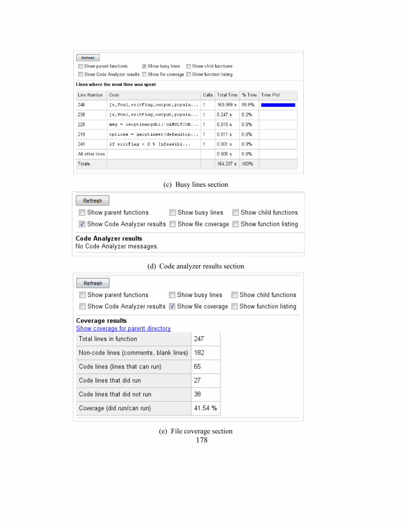
178

(c) Busy lines section

(d) Code analyzer results section

(e) File coverage section

179

(f) Function listing section

Figure F-2: Different sections of the Profile Detail report

One extension of the profile function is parallel profiler (mpiprofile) which is useful for parallel

jobs. This profiler determines the amount of time that each worker spends in order to perform its

task, and the time needed for communication between workers. Unfortunately, this type of profiler

does not support parfor-loops which is the parallel part used in this research.

Appendix G – Problem Faced Using SimEvents Simulation Tool and Parallel

Computing

There were two main issues in performing parallel computing pertinent to memory leakage and

speed problem.

G.1 Memory leakage

Once the model was run on the server machine, an error regarding the memory of the computer

appeared in MATLAB after some generations causing the failure of the program. One limitation

180

of using this machine was the relatively small size of its available RAM (48 GB). In this model,

the simOut data was appended into a cell array to save output data of the simulation for the

specified number of iterations where each iteration increases its size by about 380KB. For

example, over 1000 iterations that sums to 380MB which can be a sizeable amount of memory

topped with the memory of MATLAB for the 6 GB machine. To solve this problem, virtual

memory of the computer was increased to a very large number (like 100 GB) to use its capability

of saving more data.

Memory leakage can be produced due to use of Time-Based Function-Call Generator blocks in

the simulation model. Each block is configured to generate a certain number of function-calls only

at the beginning of the simulation. This block is usually connected to an Event-Based Entity

Generator which senses the function-call and generates that many entities when the simulation

starts. Such a scheme is usually used to preload a queue at the start of simulation.

In order to prevent memory leakage during the program progress, this pattern can be replaced with

an Event-Based Sequence block connected to a Time-Based Entity Generator block which is

configured to read inter-generation times from signal port. In this case, if n entities should be

generated at the start of the simulation (e.g., number of crews = 1 to n), then the intergeneration

time sequence should be entered as below:

181

When intergeneration time is inf, the generation will stop.

G.2 Speed Problem

One main difference between Simulink and other platforms is that Simulink checks if any updates

are made to the model before every iteration which takes some time. If updates are made, it rebuilds

the model for efficiency. As this may accumulate some overhead, it is not good in the long run,

since any changes made between iterations will be taken into consideration by Simulink.

Thus, the run time of the proposed simulation model was significantly long which shows that some

modifications are needed to fix this problem and increase the simulation speed to maximum. These

modifications are listed below:

1. Eliminate Timed to Event and Event to Timed Signal Gateway blocks

This model is purely a discrete event model with no continuous dynamics. Hence the use of these

gateway blocks should be avoided. If an event-based signal is converted to a time-based signal

using such a block then this causes extra time hits during the simulation because Simulink assumes

that the value of the signal could be continuously changing and tries to simulate these changes.

However, the signal will never change between events because its source is an event, and as such,

blocks connected to this signal need only be run when an event occurs, not at each time step of the

simulation. The motivation for inserting this gateway block in the first place was because after

running the model an error appeared asking for converting the signal from event-based to time-

based in order to use the Stop Simulation block. But instead of inserting the gateway, the Stop

182

Simulation block can be placed inside of an Atomic Subsystem and then SimEvents will run the

Atomic Subsystem only when an event occurs.

2. Eliminate some Discrete Event To Workspace blocks

All Discrete Event to Workspace blocks commented out except the ones that are needed to observe

the simulation output because every additional logging block introduces some overhead. Also, any

logging blocks that were inserted for debugging can be kept commented out during the test.

3. Eliminate all Attribute Function blocks

All of the Attribute Function blocks in the model are removed and replaced with equivalent

Simulink and SimEvents blocks. The Attribute Function block uses another MATLAB Function

block in which a MATLAB code has been written to compute attribute values. During compilation,

this block generates a MEX (MATLAB executable) file (Dynamic Link Library (DLL)) and during

simulation if calls that DLL at each time step. This greatly increases compilation time. Depending

on what the MATLAB code does, this could increase simulation time also.

In this case, the MATLAB code was only doing some basic arithmetic operations. So the cost of

calling a DLL is comparable to the cost of running the MATLAB code and this slows down the

simulation. If there is a more complicated MATLAB function then perhaps it would have been

worth the cost of calling a DLL at each time step. Replacing such blocks with equivalent Simulink

interpretations will reduce model run-time greatly.

183

4. Turning off all debugging-related options

Also, all debugging-related options were turned off from the Simulation Target pane of the model's

Configuration Parameters dialog to save more time. Using these changes, the maximum possible

efficiency can be obtained in Simulink.

5. Defining integer decision variables

In addition, the variables of the multi-objective optimization problem are defined to be only

integers by creating custom creation, mutation and crossover functions that generate only integer

outputs for the required variables.

The general idea here is to take an approach based on a continuous parameter space strategy and

make it discrete, based on well-placed calls to the rounding functions, FLOOR and CEIL.

G.3 Problem with C-compiler:

After running the proposed model on 4-core desktop machine, the model was run on the server

machine with properties as: Server/Intel Xeon CPU E5540 @ 2.53 GHz, 48 GB Random Access

Memory (RAM), and running Windows 2010 Dell computer with 12 cores.

The first problem in this case was an error about the non-existence of the C-compiler of the

Simulink Toolbox which means that the server machine on which MATLAB is running, either

does not have a supported C-compiler installed on it, or MATLAB has not been set-up to use the

relevant compiler. In order to set MATLAB up to use a supported compiler, the “mex-setup”

184

command was run at the command line which showed that there was not any supported C-compiler

installed on the server machine. Therefore, “Microsoft Visual C++ 2010 Professional” compiler

(Table G-1) was installed to resolve the issue.

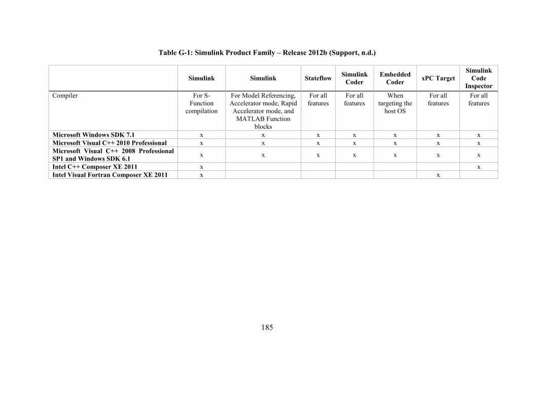
http://msdn.microsoft.com/en-us/vstudio/bb984878.aspx

185

Table G-1: Simulink Product Family – Release 2012b (Support, n.d.)

Simulink Simulink Stateflow Simulink

Coder

Embedded

Coder xPC Target

Simulink

Code

Inspector

Compiler For S-

Function

compilation

For Model Referencing,

Accelerator mode, Rapid

Accelerator mode, and

MATLAB Function

blocks

For all

features

For all

features

When

targeting the

host OS

For all

features

For all

features

Microsoft Windows SDK 7.1 x x x x x x x

Microsoft Visual C++ 2010 Professional x x x x x x x

Microsoft Visual C++ 2008 Professional

SP1 and Windows SDK 6.1 x x x x x x x

Intel C++ Composer XE 2011 x x

Intel Visual Fortran Composer XE 2011 x x

http://www.microsoft.com/downloads/details.aspx?FamilyID=6b6c21d2-2006-4afa-9702-529fa782d63b&displaylang=en

http://msdn.microsoft.com/en-us/vstudio/bb984878.aspx

http://www.microsoft.com/downloads/details.aspx?FamilyId=FBEE1648-7106-44A7-9649-6D9F6D58056E&displaylang=en

http://www.microsoft.com/downloads/details.aspx?FamilyId=FBEE1648-7106-44A7-9649-6D9F6D58056E&displaylang=en

http://www.microsoft.com/downloads/details.aspx?FamilyId=F26B1AA4-741A-433A-9BE5-FA919850BDBF&displaylang=en

performance analysis of simulation-based multi-objective ... · pdf fileiii abstract...

Documents