1“People Hearing Without Listening:”An Introduction To Compressive Sampling

Emmanuel J. Candes and Michael B. Wakin

Applied and Computational MathematicsCalifornia Institute of Technology, Pasadena CA 91125

I. INTRODUCTION

The conventional approach to sampling signals or images follows the celebrated Shannon sampling

theorem: the sampling rate must be at least twice the maximum frequency present in the signal (the

so-called Nyquist rate). In fact, this principle underlies nearly all signal acquisition protocols used in

consumer audio and visual electronics, medical imaging devices, radio receivers, and so on. In the field

of data conversion, for example, standard analog-to-digital converter (ADC) technology implements the

usual quantized Shannon representation: the signal is uniformly sampled at or above the Nyquist rate.

This paper surveys the theory of compressive sampling also known as compressed sensing, or CS,

a novel sensing/sampling paradigm that goes against the common wisdom in data acquisition. The CS

theory asserts that one can recover certain signals and images from far fewer samples or measurements

than traditional methods use. To make this possible, compressive sampling relies on two tenets, namely,

sparsity, which pertains to the signals of interest, and incoherence, which pertains to the sensing modality.

• Sparsity expresses the idea that the “information rate” of a continuous time signal may be much

smaller than suggested by its bandwidth, or that a discrete-time signal depends on a number of

degrees of freedom which is comparably much smaller than its (finite) length. More precisely,

compressive sampling exploits the fact that many natural signals are sparse or compressible in the

sense that they have concise representations when expressed in the proper basis Ψ.

• Incoherence extends the duality between time and frequency and expresses the idea that objects

having a sparse representation in Ψ must be spread out in the domain in which they are acquired,

just as a Dirac or a spike in the time domain is spread out in the frequency domain. Put differently,

incoherence says that unlike the signal of interest, the sampling/sensing waveforms have an extremely

dense representation in Ψ.

Email: {emmanuel,wakin}@acm.caltech.edu.

DRAFT

The crucial observation is that one can design efficient sensing or sampling protocols that capture the

useful information content embedded in a sparse signal and condense it into a small amount of data.

These protocols are nonadaptive and simply require correlating the signal with a small number of fixed

waveforms that are incoherent with the basis offering a concise description of the signal. (Otherwise

there is no dependence of the measurement process on the signal itself.) Further, there is a way to use

numerical optimization to reconstruct the full-length signal from the small amount of collected data. In

other words, CS is a very simple and efficient signal acquisition protocol which samples—in a signal

independent fashion—at a low rate and later uses computational power for reconstruction from what

appears to be an incomplete set of measurements.

Our intent in this paper is to overview the basic CS theory which emerged in the works [1] and [2],

[3], present the key mathematical ideas underlying this theory, and survey a couple of important results

in the field. Our goal here is to explain this theory as plainly as possible, and so our paper is mainly

of a tutorial nature. One of the charms of this theory is that it draws from various subdisciplines within

the applied mathematical sciences—most notably probability theory. In this review, we have decided to

highlight this aspect and especially the fact that randomness can—perhaps surprisingly—be used as a

very effective sensing mechanism. Finally, we will discuss significant implications and explain why CS

is a concrete protocol for sensing and compressing data simultaneously (this is the origin of the name),

and conclude our tour by reviewing important applications.

II. THE SENSING PROBLEM

In this paper, we discuss sensing mechanisms in which information about a signal f(t) is obtained by

linear functionals recording the values

yk = 〈f, ϕk〉, k = 1, . . . ,m. (1)

That is, we simply correlate the object we wish to acquire with the waveforms ϕk(t). This is a standard

setup. If the sensing waveforms are Dirac delta functions (spikes) for example, then y is a vector of

sampled values of f in the time or space domain. If the sensing waveforms are indicator functions of

pixels, then y is the image data typically collected by sensors in a digital camera. Finally, if the sensing

waveforms are sinusoids, then y is a vector of Fourier coefficients; this corresponds to the sensing modality

in use in Magnetic Resonance imaging (MRI). Other examples abound.

Although one could develop a CS theory of continuous time/space signals, we restrict our attention to

discrete signals f ∈ Rn. The reason is essentially twofold: first, this is conceptually simpler and second,

the available CS theory is far more developed in this setting. (We briefly revisit the problem of analog CS

2

in Section VII.) Having said this, we are then interested in undersampled situations in which the number

m of available measurements is much smaller than the dimension n of the signal f . Such problems are

extremely common for a variety of reasons. For instance, the number of sensors may be limited. Or the

measurements may be extremely expensive as in certain imaging processes via neutron scattering. Or the

sensing process may be slow so that one can only measure the object a few times as in MRI. And so on.

These circumstances raise important questions. Is accurate reconstruction possible from m � n

measurements only? Is it possible to design m � n sensing waveforms to capture almost all the

information about f? And how can one approximate f from this information? Admittedly, this state of

affairs looks rather daunting, as one would need to solve an underdetermined linear system of equations.

Letting A denote the m × n sensing matrix with the vectors ϕ∗1, . . . , ϕ∗m as rows (a∗ is the complex

transpose of a), the process of recovering f ∈ Rn from y = Af ∈ Rm is ill-posed in general when

m < n: there are infinitely many candidate signals f for which Af = y. But one could perhaps imagine

a way out by relying on realistic models of objects f which naturally exist. This is the topic of the

remainder of the paper.

III. INCOHERENCE AND THE SENSING OF SPARSE SIGNALS

This section presents the two fundamental premises underlying CS: sparsity and incoherence.

A. Sparsity

Many natural signals have concise representations when expressed in a convenient basis. Consider,

for example, the image in Figure 1 and its wavelet transform. Although nearly all pixels in the original

image have nonzero values, the wavelet coefficients offer a concise summary: most wavelet coefficients

are small, and the relatively few large coefficients capture most of the information about the object.

Mathematically speaking, we have a vector f ∈ Rn (such as the n-pixel image in Figure 1) which we

expand in an orthonormal basis (such as a wavelet basis) Ψ = [ψ1 ψ2 · · ·ψn] as follows:

f(t) =n∑i=1

xiψi(t), (2)

where x is the coefficient sequence of f , xi = 〈f, ψi〉. It will be convenient to express f as Ψx (where Ψ

is the n×n matrix with ψ1, . . . , ψn as columns). The implication of sparsity is now clear: when a signal

has a sparse expansion, one can discard the small coefficients without much perceptual loss. Formally,

consider fS(t) obtained by keeping only the terms corresponding to the S largest values of (xi) in the

expansion (2). By definition, fS := ΨxS , where here and below, xS is the vector of coefficients (xi) with

all but the largest S set to zero. This vector is sparse in a strict sense since all but a few of its entries

3

0 2 4 6 8 10x 105

!1

!0.5

0

0.5

1

1.5

2x 104 Wavelet Coefficients

Fig. 1. Original megapixel image with pixel values in the range [0,255] and its wavelet transform coefficients (arranged

in a random order for enhanced visibility). Relatively few wavelet coefficients capture most of the signal energy. Many

such images are highly compressible and the rightmost image shows the reconstruction obtained by zeroing out all the

coefficients in the wavelet expansion but the 25,000 largest (pixel values below 0 and above 255 are set to 0 and 255

respectively). The difference with the original picture is hardly noticeable.

are zero; we will call S-sparse such objects with at most S nonzero entries. Since Ψ is an orthobasis,

we have

‖f − fS‖`2 = ‖x− xS‖`2 ,

and if x is sparse or compressible in the sense that the sorted magnitudes of the coefficients in x decay

quickly, then x is well-approximated by xS and, therefore, the error ‖f−fS‖`2 is small. In plain terms, one

can “throw away” all but perhaps a small fraction of the coefficients without much loss. Figure 1 shows

an example where the perceptual loss is hardly noticeable from a megapixel image to its approximation

obtained by throwing away 97.5% of the coefficients.

This principle is of course what underlies most modern lossy coders such as JPEG-2000 [4] and many

others, since a simple method for data compression would simply be to compute x from f and then

(adaptively) encode the locations and values of the S significant coefficients. Such a compression process

requires knowledge of all the n coefficients x, as the locations of the significant pieces of information

may not be known in advance (they are signal dependent and in our example, they will tend to be

clustered around edges in the image whose locations are a priori unknown). More generally, sparsity

is a fundamental modelling tool which permits efficient fundamental signal processing; e.g. accurate

statistical estimation and classification, efficient data compression, and so on. This paper is about a more

surprising and far-reaching implication, however, which is that signal sparsity has significant bearings on

the acquisition process itself. Sparsity determines how efficiently one can acquire signals nonadaptively.

4

B. Incoherent sampling

Suppose we are given a pair (Φ,Ψ) of orthobases of Rn. The first basis Φ is used for sensing the

object f as in (1) and the second is used to represent f . The restriction to pairs of orthobases is not

essential and will merely simplify our treatment.

Definition 3.1: The coherence between the sensing system Φ and the representation system Ψ is

µ(Φ,Ψ) =√n · max

1≤k,j≤n|〈ϕk, ψj〉|. (3)

In plain English, the coherence measures the largest correlation between any two elements of Φ and Ψ,

see also [5]. If Φ and Ψ contain correlated elements, the coherence is large. Otherwise, it is small. As for

how large and how small, observe that µ(Φ,Ψ) ∈ [1,√n]. The upper endpoint is a consequence of the

fact that the inner product |〈ϕk, ψj〉| between two unit vectors is less or equal to 1. The lower endpoint

is a consequence of Parseval relation which states that for each j,∑n

k=1 |〈ϕk, ψj〉|2 = ‖ψj‖2`2 = 1.

Compressive sampling is mainly concerned with low coherence pairs, and we now give examples of such

pairs.

In our first example, Φ is the canonical or spike basis ϕk(t) = δ(t − k) and Ψ is the Fourier basis,

ψj(t) = n−1/2ei2π jt/n. Since Φ is the sensing matrix, this corresponds to the classical sampling scheme

in time or in space. The time-frequency pair obeys µ(Φ,Ψ) = 1 and, therefore, we have maximal

incoherence. Further, spikes and sinusoids are maximally incoherent not just in 1D but in any dimension;

in 2D, 3D, etc.

Our second example takes wavelets bases for Ψ and noiselets [6] for Φ. Here, the coherence between

noiselets and Haar wavelets is√

2, and that between noiselets and Daubechies D4 and D8 wavelets

is respectively about 2.2 and 2.9 across a very wide range of sample sizes n. This extends to higher

dimensions as well. (Noiselets are also maximally incoherent with spikes and incoherent with the Fourier

basis.) Our interest in noiselets comes from the fact that (1) they are incoherent with systems providing

sparse representations of image data and other types of data, and (2) they come with very fast algorithms;

the noiselet transform runs in O(n) time, and just like the Fourier transform, the noiselet matrix does

not need to be stored to be applied to a vector. This is of crucial importance for efficient numerical

computations without which CS would not be very practical.

Finally, random matrices are largely incoherent with any fixed basis Ψ. Select an orthonormal basis

Φ uniformly at random, which can be done by orthonormalizing n vectors sampled independently and

uniformly on the unit sphere. Then with high probability, the coherence between Φ and Ψ is about√

2 log n. By extension, random waveforms (ϕk(t)) with i.i.d. entries, e.g. Gaussian or ±1 binary entries,

will also exhibit a very low coherence with any fixed representation Ψ. Note the rather strange implication

5

here; if sensing with incoherent systems is good, then efficient mechanisms ought to acquire correlations

with random waveforms, e.g. white noise!

C. Undersampling and sparse signal recovery

Ideally, we would like to measure all the n coefficients of f , but we only get to observe a subset of

these and collect the data

yk = 〈f, ϕk〉, k ∈M, (4)

where M ⊂ {1, . . . , n} is a subset of cardinality m < n. With this information, we decide to recover the

signal by `1-norm minimization; the proposed reconstruction f? is given by f? = Ψx?, where x? is the

solution to the convex optimization program (‖x‖`1 :=∑

i |xi|)

minx∈Rn ‖x‖`1 subject to yk = 〈ϕk,Ψx〉, ∀ k ∈M. (5)

That is, among all objects f = Ψx consistent with the data, we pick that whose coefficient sequence has

minimal `1 norm1.

The use of the `1 norm as a sparsity-promoting function traces back several decades. A leading early

application was reflection seismology, in which a sparse reflection function (indicating meaningful changes

between subsurface layers) was sought from bandlimited data [7], [8]. However, `1-minimization is not

the only way to recover sparse solutions; other methods, such as greedy algorithms [9], have also been

proposed.

Our first result asserts that when f is sufficiently sparse, the recovery via `1-minimization is provably

exact.

Theorem 1 ( [10]): Fix f ∈ Rn and suppose that the coefficient sequence x of f in the basis Ψ is

S-sparse. Select m measurements in the Φ domain uniformly at random. Then if

m ≥ C · µ2(Φ,Ψ) · S · log n (6)

for some positive constant C, the solution to (5) is exact with overwhelming probability2.

We wish to make three comments. (1) The role of the coherence is completely transparent; the smaller the

coherence, the fewer samples are needed, hence our emphasis on low coherence systems in the previous

section. (2) One suffers no information loss by measuring just about any set of m coefficients which may

1As is well known, minimizing `1 subject to linear equality constraints can easily be recast as a linear program making

available a host of ever more efficient solution algorithms.2It is shown that the probability of success exceeds 1− δ if m ≥ C · µ2(Φ,Ψ) · S · log(n/δ). In addition, the result is only

guaranteed for nearly all sign sequences x with a fixed support, see [10] for details.

6

be far less than the signal size apparently demands. If µ(Φ,Ψ) is equal or close to one, then on the order

of S log n samples suffice instead of n. (3) The signal f can be exactly recovered from our condensed

dataset by minimizing a convex functional which does not assume any knowledge about the number

of nonzero coordinates of x, their locations, and their amplitudes which we assume are all completely

unknown a priori. We just run the algorithm and if the signal happens to be sufficiently sparse, exact

recovery occurs.

The theorem indeed suggests a very concrete acquisition protocol; sample nonadaptively in an inco-

herent domain and invoke linear programming after the acquisition step. Following this protocol would

essentially acquire the signal in a compressed form. All that is needed is a decoder to “decompress” this

data; this is the role of `1 minimization.

In truth, this incoherent sampling theorem extends an earlier result about the sampling of spectrally

sparse signals [1], which perhaps triggered the many CS developments we have witnessed and continue

to witness today. Suppose that we are interested in sampling ultra-wideband but spectrally sparse signals

of the form

f(t) =n−1∑j=0

xj ei2πjt/n, t = 0, . . . , n− 1,

where n is very large but where the number of nonzero components xj is less or equal to S (which we

should think of as comparably small). We do not know which frequencies are active nor do we know the

amplitudes on this active set. Because the active set is not necessarily a subset of consecutive integers,

the Nyquist/Shannon theory is mostly unhelpful (since one cannot restrict the bandwidth a priori, one

may be led to believe that all n time samples are needed). In this special instance, Theorem 1 claims

that one can reconstruct a signal with arbitrary and unknown frequency support of size S from on the

order of S log n time samples, see [1]. What is more, these samples do not have to be carefully chosen;

almost any sample set of this size will work. An illustrative example is provided in Figure 2. For other

types of theoretical results in this direction using completely different ideas, see [11] and [12].

It is now time to discuss the role played by probability in all of this. The key point is that in order to

get useful and powerful results, one needs to resort to a probabilistic statement since one cannot hope

for comparable results holding for all measurement sets of size m. Here is why. There are special sparse

signals which vanish nearly everywhere in the Φ domain. In other words, one can find sparse signals f

and very large subsets of size almost n (e.g. n − S) for which yk = 〈f, ϕk〉 = 0 for all k ∈ M . The

interested reader may want to check the example of the Dirac comb discussed in [13] and [1]. On the one

hand, given such subsets, one would get to see a stream of zeros and no algorithm whatsoever would of

course be able reconstruct the signal. On the other hand, the theorem guarantees that the fraction of sets

7

0 200 400 600−2

−1

0

1

2Sparse signal

original

0 200 400 600−2

−1

0

1

2

l1 recovery

originalrecovered

0 200 400 600−2

−1

0

1

2

l2 recovery

originalrecovered

Fig. 2. A sparse real valued signal (left) and its reconstruction from 60 (complex) valued Fourier coefficients by

`1 minimization (middle). The reconstruction is exact. The rightmost plot shows the minimum energy reconstruction

obtained by substituting the `1 norm with the `2 norm; `1 and `2 give wildly different answers. The `2 solution does

not provide a reasonable approximation to the original signal.

for which exact recovery does not occur is truly negligible (a large negative power of n). Thus, we only

have to tolerate a probability of failure which is extremely small. For practical purposes, the probability

of failure is zero provided that the sampling size is sufficiently large.

Interestingly, the study of special sparse signals discussed above also shows that one needs at least on

the order of µ2 · S · log n samples as well3. With fewer samples, the probability that information may

be lost is just too high and reconstruction by any method, no matter how intractable, is impossible. In

summary, when the coherence is 1, say, we do not need more than S log n samples but we cannot do

with fewer either.

We conclude this section with an incoherent sampling example, and consider the sparse Comedian

image of Figure 3, the same as the “compressed” megapixel image of Figure 1 (right). We recall that

the object under study is sparse since it has only 25,000 nonzero wavelet coefficients. We then acquire

information by taking 96,000 incoherent measurements (we defer the reader to [10] for the particulars of

these measurements) and solve (5). This example shows that a number of samples just about 4 times the

sparsity level suffices. Many researchers have reported on similar empirical successes. There is de facto

a known 4-to-1 practical rule which says that for exact recovery, one needs about 4 incoherent samples

per unknown nonzero term.

3We are well aware that there exist subsets of cardinality 2S in the time domain which can reconstruct any S-sparse signal

in the frequency domain. Simply take 2S consecutive time points, see Section VI and [12], [14] for example. But this is not

what our claim is about. We want that most sets of certain size provide exact reconstruction.

8

Fig. 3. Original 25,000-sparse image (left) and its reconstruction from 96,000 undersampled incoherent measure-

ments. The minimum-`1 recovery is perfect.

IV. ROBUST COMPRESSIVE SAMPLING

We have shown that one could recover sparse signals from just a few measurements but in order to

be really powerful, CS needs to be able to deal with both nearly sparse signals and with noise.

1) First, general objects of interest are not exactly sparse but approximately sparse. The issue here

is whether or not it is possible to obtain accurate reconstructions of such objects from highly

undersampled measurements.

2) Second, in any real application measured data will invariably be corrupted by at least a small

amount of noise as sensing devices do not have infinite precision. It is therefore imperative that

CS be robust vis a vis such nonidealities. At the very least, small perturbations in the data should

cause small perturbations in the reconstruction.

This section examines these two issues simultaneously. Before we begin, however, it will ease the

exposition to consider the abstract problem of recovering a vector x ∈ Rn from data y of the form

y = Ax+ z, (7)

where A is an m×n “sensing matrix” giving us information about x, and z is a stochastic or deterministic

unknown error term. The setup of the last section is of this form since with f = Ψx and y = RΦf (R is

the m× n matrix extracting the sampled coordinates in M ), one can write y = Ax, where A = RΦ Ψ.

Hence, one can work with the abstract model (7) bearing in mind that x may be the coefficient sequence

of the object in a proper basis.

A. Restricted isometries

In this section, we introduce a key notion that has proved to be very useful to study the general

robustness of compressive sampling; the so-called restricted isometry property (RIP) [15].

9

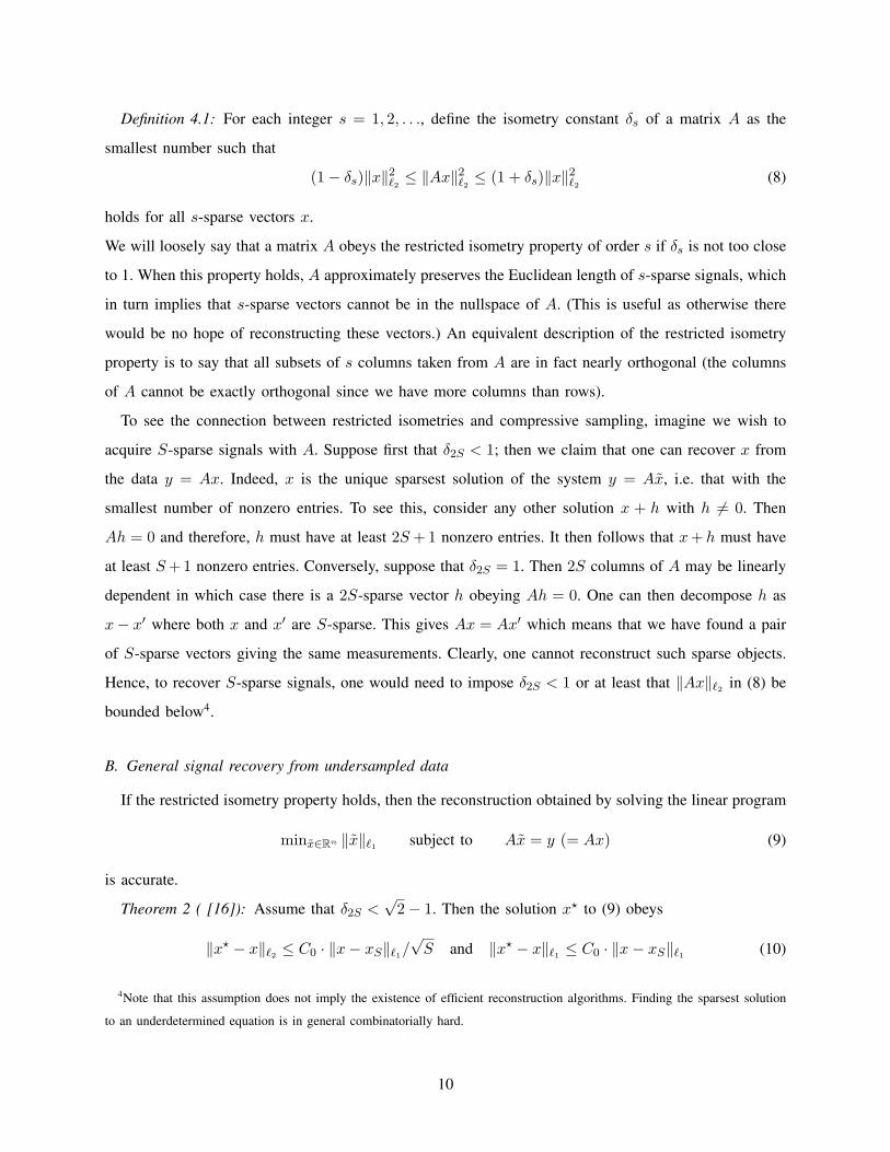
Definition 4.1: For each integer s = 1, 2, . . ., define the isometry constant δs of a matrix A as the

smallest number such that

(1− δs)‖x‖2`2 ≤ ‖Ax‖2`2 ≤ (1 + δs)‖x‖2`2 (8)

holds for all s-sparse vectors x.

We will loosely say that a matrix A obeys the restricted isometry property of order s if δs is not too close

to 1. When this property holds, A approximately preserves the Euclidean length of s-sparse signals, which

in turn implies that s-sparse vectors cannot be in the nullspace of A. (This is useful as otherwise there

would be no hope of reconstructing these vectors.) An equivalent description of the restricted isometry

property is to say that all subsets of s columns taken from A are in fact nearly orthogonal (the columns

of A cannot be exactly orthogonal since we have more columns than rows).

To see the connection between restricted isometries and compressive sampling, imagine we wish to

acquire S-sparse signals with A. Suppose first that δ2S < 1; then we claim that one can recover x from

the data y = Ax. Indeed, x is the unique sparsest solution of the system y = Ax, i.e. that with the

smallest number of nonzero entries. To see this, consider any other solution x + h with h 6= 0. Then

Ah = 0 and therefore, h must have at least 2S + 1 nonzero entries. It then follows that x+ h must have

at least S+ 1 nonzero entries. Conversely, suppose that δ2S = 1. Then 2S columns of A may be linearly

dependent in which case there is a 2S-sparse vector h obeying Ah = 0. One can then decompose h as

x− x′ where both x and x′ are S-sparse. This gives Ax = Ax′ which means that we have found a pair

of S-sparse vectors giving the same measurements. Clearly, one cannot reconstruct such sparse objects.

Hence, to recover S-sparse signals, one would need to impose δ2S < 1 or at least that ‖Ax‖`2 in (8) be

bounded below4.

B. General signal recovery from undersampled data

If the restricted isometry property holds, then the reconstruction obtained by solving the linear program

minx∈Rn ‖x‖`1 subject to Ax = y (= Ax) (9)

is accurate.

Theorem 2 ( [16]): Assume that δ2S <√

2− 1. Then the solution x? to (9) obeys

‖x? − x‖`2 ≤ C0 · ‖x− xS‖`1/√S and ‖x? − x‖`1 ≤ C0 · ‖x− xS‖`1 (10)

4Note that this assumption does not imply the existence of efficient reconstruction algorithms. Finding the sparsest solution

to an underdetermined equation is in general combinatorially hard.

10

for some constant C0, where xS is the vector x with all but the largest S components set to zero5.

The conclusions of this theorem are stronger than those of Theorem 1. If x is S-sparse, then x = xS and,

therefore, the recovery is exact. But this new theorem deals with all signals. If x is not S-sparse, then

(10) asserts that the quality of the recovered signal is as good as if one knew ahead of time the location

of the S largest values of x and decided to measure those directly. In other words, the reconstruction is

nearly as good as that provided by an oracle which, with full and perfect knowledge about the object,

would extract the S most significant pieces of information for us.

Another striking difference with our earlier result is that it is deterministic; it involves no probability.

If we are fortunate enough to hold a sensing matrix A obeying the hypothesis of the theorem, we may

apply it, and we are then guaranteed to recover all sparse S-vectors exactly, and essentially the S-largest

entries of all vectors otherwise; i.e. there is no probability of failure. Further, since the same sensing

matrix A works for all vectors in Rn, it is often referred to as universal.

What is missing at this point is the relationship between S (the number of components one can

effectively recover) obeying the hypothesis and m the number of measurements or rows of the matrix.

To derive powerful results, we would like to find matrices obeying the restricted isometry property with

values of S close to m. Can one design such matrices? In the next section, we will show that this is

possible, but first we examine the robustness of CS vis a vis data corruption.

C. Robust signal recovery from noisy data

We are given noisy data as in (7) and use `1 minimization with relaxed constraints for reconstruction:

min ‖x‖`1 subject to ‖Ax− y‖`2 ≤ ε, (11)

where ε bounds the amount of noise in the data6. Problem (11) is often called the LASSO after [21];

see also [22]. To the best of our knowledge, it was first proposed in [8]. This is again a special convex

problem, a second-order cone program to be exact, and many efficient algorithms exist for solving it.

Theorem 3 ( [16]): Assume that δ2S <√

2− 1. Then the solution x? to (11) obeys

‖x? − x‖`2 ≤ C0 · ‖x− xS‖`1/√S + C1 · ε (12)

for some constants C0 and C17.

5As stated, this result is due to the first author [17] and yet unpublished, see [16] and also [18] for related formulations.6One could also consider recovery programs such as the Dantzig selector [19] or a combinatorial optimization program

proposed by Haupt and Nowak [20]; both algorithms have provable results in the case where the noise is Gaussian with bounded

variance.7Again, this theorem is unpublished as stated, and is a variation on the result found in [16].

11

−1 0 1 2

−1.5

−1

−0.5

0

0.5

1

1.5

2

Original signal versus reconstruction

xx∗

Fig. 4. A signal x (horizontal axis) and its reconstruction x? (vertical axis) obtained via (11). In this example, n = 512

and m = 256. The signal is 64-sparse. In the model (7), the sensing matrix has i.i.d. N(0, 1/m) entries and z is a

Gaussian white noise vector. The noise level is adjusted so that ‖Ax‖`2/‖z‖`2 = 5. Here, ‖x? − x‖`2 ≈ 1.3 · ε.

This can hardly be simpler. The reconstruction error is bounded by the sum of two terms. The first is

the error which would occur if one had noiseless data. The second is just proportional to the noise level.

Further, the constants C0 and C1 are typically small. With δ2S = 1/4 for example, C0 ≤ 5.5 and C1 ≤ 6.

Figure 4 shows a reconstruction from noisy data.

This last result establishes CS as a practical and efficient sensing mechanism. It is robust in the sense

that it works with all kinds of not necessarily sparse signals and in the sense that it handles noise

gracefully. What remains to be done is to design efficient sensing matrices obeying the RIP. This is the

object of the next section.

V. RANDOM SENSING

Returning to the definition of the restricted isometry property, we would like to find sensing matrices

with the property that column vectors taken from arbitrary subsets are nearly orthogonal. The larger these

subsets, the better. This is where randomness re-enters the picture.

Consider the following sensing matrices:

1) Form A by sampling n column vectors uniformly at random on the unit sphere of Rm.

2) Form A by sampling i.i.d. entries from the normal distribution with mean zero and variance 1/m.

3) Form A by sampling a random projection P as in Section III-B and normalize: A =√

nm P .

4) Form A by sampling i.i.d. entries from a symmetric Bernoulli distribution (P(Ai,j = ±1/√m) = 1

2)

or other subgaussian distribution.

12

Then with overwhelming probability, all these matrices obey the restricted isometry property (i.e. the

condition of our theorem) provided that

m ≥ C · S log(n/S), (13)

where C is some constant depending on each instance. The claim for 1), 2) and 3) uses fairly standard

results in probability theory; arguments for 4) are more subtle, see [23] and the work of Pajor and his

coworkers, e.g. [24]. In all these examples, the probability of sampling a matrix not obeying the RIP

when (13) holds is exponentially small in m. Interestingly, there are no measurement matrices and no

reconstruction algorithm whatsoever which can give the conclusions of Theorem 2 with substantially

fewer samples than the left-hand side of (13) [2], [3]. In that sense, using the sensing matrices above

together with `1 minimization is a near-optimal sensing strategy.

One can also establish the restricted isometry property for pairs of orthobases as in Section III. With

A = RΦΨ where R extracts m coordinates uniformly at random, it is sufficient to have

m ≥ C · S (log n)4, (14)

for the property to hold with large probability, see [25] and [2]. If one wants a probability of failure no

larger than O(n−β) for some β > 0, then the best known exponent in (14) is 5 instead of 4 (it is believed

that (14) holds with just log n). This proves that one can stably and accurately reconstruct nearly sparse

signals from dramatically undersampled data in an incoherent domain.

Finally, the restricted isometry property can also hold for sensing matrices A = ΦΨ, where Ψ is an

arbitrary orthonormal basis and Φ is an m × n measurement matrix drawn randomly from a suitable

distribution. If one fixes the basis Ψ and populates the measurement matrix Φ as in 1)—4), then with

overwhelming probability, the matrix A = ΦΨ obeys the RIP provided that

m ≥ C · S log(n/S), (15)

where again C is some constant depending on each instance. These random measurement matrices Φ are

in a sense universal [23]; the sparsity basis need not even be known when designing the measurement

system!

VI. WHAT IS COMPRESSIVE SAMPLING?

Data acquisition typically works as follows: massive amounts of data are collected only to be—in

large part—discarded at the compression stage, which is usually necessary for storage and transmission

purposes. In the language of this paper, one acquires a high-resolution pixel array f , computes the

13

complete set of transform coefficients, encode the largest coefficients and discard all the others, essentially

ending up with fS . This process of massive data acquisition followed by compression is extremely wasteful

(one can think about a digital camera which has millions of imaging sensors, the pixels, but eventually

encodes the picture in just a few hundred kilobytes).

CS operates very differently, and performs as “if it were possible to directly acquire just the important

information about the object of interest.” By taking about O(S log(n/S)) random projections as in

Section V, one has enough information to reconstruct the signal with an accuracy at least as good as that

provided with fS , the best S-term approximation—the best compressed representation—of the object.

In other words, CS data acquisition protocols essentially translate analog data into already compressed

digital form so that one can—at least in principle—obtain super-resolved signals from just a few sensors.

All that is needed after the acquisition step is to “decompress” the measured data. What is unexpected

is that the acquisition step is fixed and in particular, does not try to figure out the structure of the signal

at all; like hearing without listening.

There are some superficial similarities between CS and ideas in coding theory and more precisely with

the theory and practice of Reed-Solomon codes [26]. In a nutshell and in the context of this paper, it

is well known that one can adapt ideas from coding theory to establish the following: one can uniquely

reconstruct any S-sparse signal from the data of its first 2S Fourier coefficients8,

yk =n−1∑t=0

xt e−i2π kt/n, k = 0, 1, 2, . . . , 2S − 1, (16)

or from any set of 2S consecutive frequencies for that matter (the computational cost for the recovery

is essentially that of solving an S × S Toeplitz system and of taking an n-point FFT). Does this mean

that one can use this technique to sense compressible signals? The answer is negative and there are two

main reasons for this. First, the problem is that Reed-Solomon decoding is an algebraic technique, which

cannot deal with nonsparse signals (the decoding finds the support by rooting a polynomial); second,

the problem of finding the support of a signal—even when the signal is exactly sparse—from its first

2S Fourier coefficients is extraordinarily ill posed (the problem is the same as that of extrapolating a

high degree polynomial from a small number of highly clustered values). Tiny perturbations of these

coefficients will give completely different answers so that with finite precision data, reliable estimation

of the support is practically impossible. Whereas purely algebraic methods ignore the conditioning of

information operators, having well-conditioned matrices, which are crucial for accurate estimation, is a

central concern in CS as evidenced by the role played by restricted isometries.

8This was actually known much earlier.

14

VII. APPLICATIONS

The fact that a compressible signal can be captured efficiently using a number of incoherent measure-

ments that is proportional to its information level S � n has implications which are far-reaching and

concern a number of possible applications:

• Data compression. In some situations, the sparse basis Ψ may be unknown at the encoder or

impractical to implement for data compression. As we discussed in Section V, however, a randomly

designed Φ can be considered a universal encoding strategy, as it need not be designed with regards

to the structure of Ψ. (The knowledge and ability to implement Ψ are required only for the decoding

or recovery of f .) This universality may be particularly helpful for distributed source coding in multi-

signal settings such as sensor networks [27]. We refer the reader to papers by Nowak et al. and

Goyal elsewhere in this issue for related discussions.

• Channel coding. As explained in [15], CS principles (sparsity, randomness, and convex optimization)

can be turned around and applied to design fast error correcting codes over the reals to protect from

errors during transmission.

• Inverse problems. In still other situations, the only way to acquire f may be to use a measurement

system Φ of a certain modality. However, assuming a sparse basis Ψ exists for f that is also incoherent

with Φ, then efficient sensing will be possible. One such application involves MR angiography [1]

and other types of MR setups [28], where Φ records a subset of the Fourier transform, and the

desired image f is sparse in the time or wavelet domains. Elsewhere in this issue, Lustig et al.

discuss this application in more depth.

• Data acquisition. Finally, in some important situations the full collection of n discrete-time samples

of an analog signal may be difficult to obtain (and possibly difficult to subsequently compress).

Here, it could be helpful to design physical sampling devices that directly record discrete, low-rate

incoherent measurements of the incident analog signal.

The last of these bullets suggests that mathematical and computational methods could have an enormous

impact in areas where conventional hardware design has significant limitations. For example, conventional

imaging devices that use CCD or CMOS technology are limited essentially to the visible spectrum.

However, a CS camera [29] that collects incoherent measurements using a digital micromirror array (and

requires just one photosensitive element instead of millions) could significantly expand these capabilities.

Elsewhere in this issue, Baraniuk et al. describe this camera in more depth.

Along these same lines, part of our research has focused on advancing devices for “analog-to-information”

(A/I) conversion of high-bandwidth signals (see also the paper by Healy et al. in this issue). Our

15

goal is to help alleviate the pressure on conventional analog-to-digital conversion technology, which

is currently limited to sample rates on the order of 1GHz. As an alternative, we have proposed two

specific architectures for A/I in which a discrete, low-rate sequence of incoherent measurements can be

acquired from a high-bandwidth analog signal. To a high degree of approximation, each measurement

yk can be interpreted as the inner product 〈f, ϕk〉 of the incident analog signal f against an analog

measurement waveform ϕk. As in the discrete CS framework, our preliminary results suggest that analog

signals obeying a sparse or compressible model (in some analog dictionary Ψ) can be captured efficiently

using these devices at a rate proportional to their information level instead of their Nyquist rate. Of course,

there are challenges one must address when applying the discrete CS methodology to the recovery of

sparse analog signals. A thorough treatment of these issues would be beyond the scope of this short

article and as a first cut, one might simply accept the idea that in many cases, discretizing/sampling the

sparse dictionary allows for suitable recovery.

Our two architectures are as follows:

1) Non-uniform Sampler (NUS). Our first architecture simply digitizes the signal at randomly sam-

pled time points. That is, yk = f(tk) = 〈f, δtk〉. In effect, these random or pseudo-random time

points are obtained by jittering nominal (low-rate) sample points located on a regular lattice. Due

to the incoherence between spikes and sines, this architecture can be used to sample signals having

sparse frequency spectra far below their Nyquist rate. There are of course tremendous benefits

associated with a reduced sampling rate as this provides added circuit settling time and has the

effect of reducing the noise level.

2) Random Pre-integration (RPI). Our second architecture is applicable to a wider variety of sparsity

domains, most notably those signals having a sparse signature in the time-frequency plane. Whereas

it may not be possible to digitize an analog signal at a very high rate rate, it may be quite possible to

change its polarity at a high rate. The idea of the RPI architecture (see Figure 5) is then to multiply

the signal by a pseudo-random sequence of plus and minus ones, integrate the product over time

windows, and digitize the integral at the end of each time interval. This is a parallel architecture

and one has several of these random multiplier-integrator pairs running in parallel using distinct or

event nearly independent pseudo-random sign sequences. In effect, the RPI architecture correlates

the signal with a bank of sequences of ±1, one of the random CS measurement processes known

to be universal.

For each of the above architectures, we have confirmed numerically (and in some cases physically) that

the system is robust to circuit nonidealities such as thermal noise, clock timing errors, interference, and

16

∫kT1,-1,1,1,-1,...

yk,1

∫kT-1,-1,-1,1,-1,...

yk,2

∫kT-1,1,-1,1,1,...

yk,P

f(t)

Fig. 5. Random Pre-integration (RPI) system for analog-to-information conversion.

amplifier nonlinearities.

The application of A/I architectures to realistic acquisition scenarios will require continued development

of CS algorithms and theory, including research into the proper dictionaries for sparse representation of

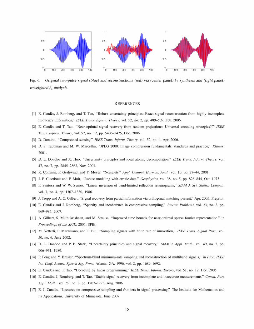
analog signals. We conclude with a final discrete example to highlight some promising recent directions.

For this experiment we take f to be a 1-D signal of length n = 512 that contains two modulated

pulses (see the left panel of Figure 6). From this signal, we collect m = 30 measurements using an

m× n measurement matrix Φ populated with i.i.d. Bernoulli ±1 entries. This is an unreasonably small

amount of data corresponding to an undersampling factor exceeding 17. For reconstruction we consider

a time-frequency Gabor dictionary Ψ that consists of a variety of sine waves time limited by Gaussian

windows, with different locations and scales. Overall the dictionary is approximately 43× overcomplete

and does not contain the two pulses that comprise f . The center panel of Figure 6 shows the result

of minimizing ‖x‖`1 such that y = ΦΨx. The reconstruction shows pronounced artifacts, and we see

‖f − f?‖`2/‖f‖`2 ≈ 0.67. However, we can virtually eliminate the reconstruction artifacts by making

two changes to the `1 recovery program. First, we instead minimize ‖Ψ∗f‖`1 subject to y = Φf . (This

variation has no effect when Ψ is an orthonormal basis.) Second, after obtaining an estimate f?, we

reweight the `1 norm and repeat the reconstruction, with a lower penalty applied to those coefficients we

anticipate to be large. The right panel of Figure 6 shows the result after four iterations of reweighting; we

see ‖f −f?‖`2/‖f‖`2 ≈ 0.022. We refer the reader to [30] for more information on these new directions.

The point here is that even though the amount of data is ridiculously small, one has nevertheless captured

most of the information contained in the signal. This is the reason why CS holds such a great promise

for current and future applications.

17

0 100 200 300 400 500−1

−0.5

0

0.5

1

0 100 200 300 400 500−1

−0.5

0

0.5

1

0 100 200 300 400 500−1

−0.5

0

0.5

1

Fig. 6. Original two-pulse signal (blue) and reconstructions (red) via (center panel) `1 synthesis and (right panel)

reweighted `1 analysis.

REFERENCES

[1] E. Candes, J. Romberg, and T. Tao, “Robust uncertainty principles: Exact signal reconstruction from highly incomplete

frequency information,” IEEE Trans. Inform. Theory, vol. 52, no. 2, pp. 489–509, Feb. 2006.

[2] E. Candes and T. Tao, “Near optimal signal recovery from random projections: Universal encoding strategies?,” IEEE

Trans. Inform. Theory, vol. 52, no. 12, pp. 5406–5425, Dec. 2006.

[3] D. Donoho, “Compressed sensing,” IEEE Trans. Inform. Theory, vol. 52, no. 4, Apr. 2006.

[4] D. S. Taubman and M. W. Marcellin, “JPEG 2000: Image compression fundamentals, standards and practice,” Kluwer,

2001.

[5] D. L. Donoho and X. Huo, “Uncertainty principles and ideal atomic decomposition,” IEEE Trans. Inform. Theory, vol.

47, no. 7, pp. 2845–2862, Nov. 2001.

[6] R. Coifman, F. Geshwind, and Y. Meyer, “Noiselets,” Appl. Comput. Harmon. Anal., vol. 10, pp. 27–44, 2001.

[7] J. F. Claerbout and F. Muir, “Robust modeling with erratic data,” Geophysics, vol. 38, no. 5, pp. 826–844, Oct. 1973.

[8] F. Santosa and W. W. Symes, “Linear inversion of band-limited reflection seismograms,” SIAM J. Sci. Statist. Comput.,

vol. 7, no. 4, pp. 1307–1330, 1986.

[9] J. Tropp and A. C. Gilbert, “Signal recovery from partial information via orthogonal matching pursuit,” Apr. 2005, Preprint.

[10] E. Candes and J. Romberg, “Sparsity and incoherence in compressive sampling,” Inverse Problems, vol. 23, no. 3, pp.

969–985, 2007.

[11] A. Gilbert, S. Muthukrishnan, and M. Strauss, “Improved time bounds for near-optimal sparse fourier representation,” in

Proceedings of the SPIE. 2005, SPIE.

[12] M. Vetterli, P. Marziliano, and T. Blu, “Sampling signals with finite rate of innovation,” IEEE Trans. Signal Proc., vol.

50, no. 6, June 2002.

[13] D. L. Donoho and P. B. Stark, “Uncertainty principles and signal recovery,” SIAM J. Appl. Math., vol. 49, no. 3, pp.

906–931, 1989.

[14] P. Feng and Y. Bresler, “Spectrum-blind minimum-rate sampling and reconstruction of multiband signals,” in Proc. IEEE

Int. Conf. Acoust. Speech Sig. Proc., Atlanta, GA, 1996, vol. 2, pp. 1689–1692.

[15] E. Candes and T. Tao, “Decoding by linear programming,” IEEE Trans. Inform. Theory, vol. 51, no. 12, Dec. 2005.

[16] E. Candes, J. Romberg, and T. Tao, “Stable signal recovery from incomplete and inaccurate measurements,” Comm. Pure

Appl. Math., vol. 59, no. 8, pp. 1207–1223, Aug. 2006.

[17] E. J. Candes, “Lectures on compressive sampling and frontiers in signal processing,” The Institute for Mathematics and

its Applications, University of Minnesota, June 2007.

18

[18] A. Cohen, W. Dahmen, and R. DeVore, “Compressed sensing and best k-term approximation,” 2006, Preprint.

[19] E. Candes and T. Tao, “The Dantzig selector: Statistical estimation when p is much larger than n,” Ann. Statist., 2005,

To appear.

[20] J. Haupt and R. Nowak, “Signal reconstruction from noisy random projections,” IEEE Trans. Inform. Theory, vol. 52, no.

9, pp. 4036–4048, 2006.

[21] R. Tibshirani, “Regression shrinkage and selection via the lasso,” J. Roy. Statist. Soc. Ser. B, vol. 58, no. 1, pp. 267–288,

1996.

[22] S. S. Chen, D. L. Donoho, and M. A. Saunders, “Atomic decomposition by basis pursuit,” SIAM J. Sci. Comput., vol. 20,

no. 1, pp. 33–61 (electronic), 1998.

[23] R. Baraniuk, M. Davenport, R. DeVore, and M. Wakin, “A simple proof of the restricted isometry property for random

matrices,” Constr. Approx., 2007, To appear.

[24] S. Mendelson, A. Pajor, and N. Tomczak-Jaegermann, “Uniform uncertainty principle for Bernoulli and subgaussian

ensembles,” 2006, Preprint.

[25] M. Rudelson and R. Vershynin, “On sparse reconstruction from Fourier and Gaussian measurements,” Communications

on Pure and Applied Mathematics (to appear), 2006.

[26] R. E. Blahut, Algebraic codes for data transmission, Cambridge University Press, 2003.

[27] D. Baron, M. B. Wakin, M. F. Duarte, S. Sarvotham, and R. G. Baraniuk, “Distributed compressed sensing,” 2005,

Preprint.

[28] M. Lustig, D. L. Donoho, and J. M. Pauly, “Rapid MR imaging with compressed sensing and randomly under-sampled

3DFT trajectories,” in Proc. 14th Ann. Mtg. ISMRM, May 2006.

[29] D. Takhar, V. Bansal, M. Wakin, M. Duarte, D. Baron, K. F. Kelly, and R. G. Baraniuk, “A compressed sensing camera:

New theory and an implementation using digital micromirrors,” in Proc. Comp. Imaging IV at SPIE Electronic Imaging,

San Jose, California, January 2006.

[30] E. J. Candes, M. B. Wakin, and S. P. Boyd, “Enhancing sparsity by reweighting `1,” Tech. Rep., California Institute of

Technology, 2007, available at http://www.acm.caltech.edu/∼emmanuel/publications.html.

19