pedro balaguer herrero - uab barcelona · pedro balaguer herrero submitted in partial fulfillment...
TRANSCRIPT
INFORMATION AND CONTROL
SUPERVISION OF ADAPTIVE/ITERATIVE SCHEMES
Pedro Balaguer Herrero
Submitted in partial fulfillment of therequirements for the degree of
Doctor Engineerat Autonomous University of Barcelona
June, 2007

Knowing ignorance is strength.Ignoring knowledge is sickness.
Lao Tzu. Tao Te Ching.
Preface
The design of a controller is a procedure which requires acquiring and pro-cessing information in order to obtain a satisfactory design. For example,system identification requires experimental data, a model structure and anidentification algorithm. Thus a nominal model plus uncertainty bounds canbe identified (i.e. a model set) which is then used to design a controller.
It is widely recognized that if new information is added to the control de-sign process, it is possible to improve the performance achieved by the designedcontroller. In fact that is the rationale behind adaptive control schemes. Adap-tive control schemes are characterized by adding new information for controldesign purposes into the control design procedure with the aim of designing abetter performing controller.
In this thesis we tackle the control design problem from the informationpoint of view. In this way the problem of designing a controller is under-stood as the problem of managing the information flow required to design aproper controller (i.e. experimental data, system identification, fundamentallimitations, control design, etc.).
The main contributions of this thesis are:
I) The control problem (i.e. the controller design problem) is posed inan information theoretic framework. Each element is endowed with aninformation measure on the basis of uncertainty information theory. Theframework permits:
i) to dissect all the available information sources for the control prob-lem. An exhaustive analysis on the information sources is con-ducted which comprises not only well known elements such as ex-perimental data but also not so well recognized elements such as a
v
priori model information (e.g. model order) and a priori controllerinformation (e.g. controller order). For example, apart from ex-perimental data, it turns out that to increase the model order orthe controller complexity can have a dramatic influence on the fi-nal designed controller, consequently they can also be regarded asinformation sources to be taken into account.
ii) Information relations among the elements of the control problem areestablished. In this way, for example, it is shown that an informa-tion increase on the model set (i.e. a model uncertainty reduction)comes necessarily by an information increase on the data set or onthe a priori model set or both. However this requirement is neces-sary but no sufficient as the identification algorithm could not makeproper use of the extra available information. The relationships arethen useful to distinguish information sources and algorithm re-quirements in order to increase the information of certain elementsbelonging to the control problem.
The above information framework is derived by first defining the controlproblem from a holistic approach. The approach is holistic as firstlyall the elements are considered and secondly the relations among theseelements are established. In this way both the elements of the controlproblem and the relationships among the elements are established andrelated with existing control theory areas. Secondly distinct definitionsof the information concept are reviewed on the basis of control theory.As a conclusion it can be seen that although the information conceptplays a major role on the control theory, a complete information the-oretic framework of control theory is still lacking. Finally distinct for-malizations of the information concept are reviewed. The UncertaintyInformation Based approach is taken in order to endow the elements ofthe holistic control problem with an information measure from whichthe already stated contributions follow.
II) On the basis of the information theoretic formalization of the controlproblem the following points are established:
i) The control design problem is considered as a problem of managingthe information flow. The information flow management point ofview permits to study and compare, under an unified framework,
distinct control design methodologies. For example, in one shotdesigns (i.e. non adaptive) the data set is kept constant meanwhilein classical adaptive control new data are periodically added to thedata set.
ii) A definition of adaptive control is given. The proposed definitiontries to amalgamate the concepts present in existing adaptive con-trol definitions. Thus a system is considered adaptive if new infor-mation is acquired and the control system is modified accordinglyin order to achieve some goal (e.g. improve performance, maintainperformance or minimize performance degradation).
iii) Iterative Control and Classical Adaptive Control are studied asspecial cases of the general adaptive control approach under theinformation theoretic framework of the control problem. For exam-ple, the only information source that is modified on classical adap-tive control is the data set. On the contrary on iterative controlschemes, apart of the data set, distinct model orders and controllerorders are obtained at each iteration depending on the model iden-tification and controller design approach taken. However the mostimportant result of adaptive control and iterative control is the lackof information monotonicity. In fact although the mentioned adap-tive control approaches incorporate new information, it is also truethat already existing information is discarded. As a consequencethe information monotonicity property is lost. The benefits of amonotonic information iterative control are shown by means of anexample of classical iterative control scheme. In the example theopen loop model discarded in the iterative control is used to designa better performing controller.
III) A new validation algorithm is proposed. The algorithm named ControlOriented Frequency Dependent Model Validation (COFDMV) is the fre-quency domain counterpart of a time domain whiteness test. The maincontributions of the algorithm are:
i) The validation result is no longer a binary “validated/invalidated”answer but more informative. In fact a model can be validated forsome frequency range but invalidated for other frequencies.
ii) The algorithm is control oriented in the sense that a model is notvalidated by itself in open loop but in closed loop. Actually whatis validated is the performance of a model-controller pair .
iii) The validation procedure is suited for iterative control schemes ingeneral as it provides the following features that help to manage theinformation flow of iterative schemes. First the algorithm is a guideto design the next experimental input. In fact if a better model ispursued around the frequency range where the former model wasinvalidated, the input should contain a high energy content aroundthose frequencies. Secondly the algorithm helps to detect possibleundermodelling problems. Finally the validation procedure gives abound on the achievable controller bandwidth with the model athand.
The main articles on international conferences the thesis has generated are:
• P. Balaguer, R. Vilanova and R. Moreno. “The Control Problem: AFramework for Holistic Design”. 14th IEEE Mediterranean Con-ference on Control and Automation, 2006.
In this work the control problem is presented from a holistic point ofview. Moreover the information flow nature of the control problem isintroduced together with a proposal to manage the information flow.
• P. Balaguer and R. Vilanova. “Is Iterative Control Wasting In-formation?”. 6th IEEE International Conference on Control and Au-tomation, 2007.
The information properties of existing iterative control schemes are dis-cussed and the problem of monotonicity is arisen. An example is pro-vided in which it is shown that taking into account disregarded informa-tion from an iterative scheme improves control performance for a widerperturbation range.
• P. Balaguer and R. Vilanova. “Frequency Dependent Approach toModel Validation”. 6th Asian Control Conference, 2006.
The paper presents de fundamentals of the frequency dependent modelvalidation algorithm
• P. Balaguer, R. Vilanova and R. Moreno. “Control Oriented Fre-quency Dependent Model Validation”. International Control Con-ference UK, 2006.
The paper endows the frequency dependent model validation approachwith control oriented issues. Residual generation structures are proposedto provide the Control Oriented Frequency Dependent Model Validationalgorithm (COFDMV).
• P. Balaguer and R. Vilanova. “Quality Assessment of Models forIterative/Adaptive Control”. 45th IEEE Conference on Decisionand Control, 2006.
The COFDMV algorithm is presented as a suited tool for model valida-tion on iterative/adaptive control schemes.
The following journal articles have been submitted to:
• P. Balaguer and R. Vilanova. “Information Characterization ofthe Control Problem. Part I: The Framework”. InternationalJournal of General Systems. (submitted)
• P. Balaguer and R. Vilanova. “Information Characterization ofthe Control Problem. Part II: Analysis of Adaptive ControlSchemes”. International Journal of General Systems. (submitted)
• P. Balaguer and R. Vilanova. “Model Validation on Adaptive Con-trol: A Frequency Dependent Approach”. International Journalof Control. (submitted)

Agraıments
Este treball ha dut molt de sacrifici i es el resultat de moltes hores de faena, ca-bilacions, soletat, satisfaccions, frustracions, derrotes, i exits. Indistintamentdel valor cientıfic o acceptacio que el treball puga tenir, cada paraula, cadafrase, cada idea es resultat de molta faena i sacrifici. Es esta faena i sacrificiel que vull dedicar-vos i amb el qual vull donar-vos les gracies.
No puc comencar per altre lloc que per el principi. Vull agrair a ma marei a mon pare tot el que han fet per mi en aquesta vida. El seu treball ha segutel meu descans, els seus patiments la meva tranquil·litat, i la meua alegria laseva. Ells m’han ensenyat les coses realment importants en la vida, les cosesa partir de les quals tot lo demes ha eixit com una simple consequencia .
Al meu iaio Vicent, per ensenyar-me el valor del coneiximent, la ciencia,la paciencia, la prudencia i el gust per la faena ben feta.
Al meu iaio Pere, per ensenyar-me a alcar-me i tornar a pujar a la bicicletaquan estava en terra, a ser atrevit, valent, apretar les dents i seguir avant.
A la meua iaia Pilar amb qui tantes vespraes vaig passar jugant a cartes.Una pena que te’n anares tan pronte.
A la meua iaia Pascuala amb qui encara tinc la sort de poder passar algunratet. Preparat que encara tenim que escriure les memories de la guerra...
A la meua germana i a Felipe.
Al meu nebot, amb la il.lusio de tot allo que fara possible.
A un home que va lluitar per la llibertat,
Onofre Domenech Taura
¡PRESENTE!
xi

A tots aquells que van fer possible les festes del poble: les histories dePascual “el chato”, l’alegria de Juan “el gordo”, els chistes de Pascualet “elcarnisser”, l’esperit de xiquet de Pepe Luis “el pintor” (q.e.d), les converses enJulio, Pascual “el gelat”, Gerardo, Rosita, Pilar, Maria, Teresita, Encarnita,Enriqueta... I tots els xiquets que allı estavem, Maria Pilar, Silvia, Ana,Hector, Laura i Julio.
Als meus amics Julio i Mayca, Manuel i Isabel, Hector i Marian, Jose “elbrother”, Javi, Pepe i Tere, Oscar i Marina, Dani i Bea i el “Tente”. Hempassat de jugar al “futbolin” a anar de boda. I el que vindra...
A Carlos i a Alberto. Dos companys excepcionals de carrera. Dos gransenginyers.
A tots els companys del Departament de Telecomunicacio i enginyeria deSistemes de la Universitat Autonoma de Barcelona. En especial a Carles perla seua comprensio, anim i per ser un gran company de despatx, a Romanper el seu companyerisme, a Monica per aguantar els problemes informatics, aChantal per la seva “simpatia”, a Sonia i Laia, les meves companyes de viatje,a Dani (tambe conegut com D.G.) per la seva paciencia davant l’adversitat,a Orlando per les seves cancons, a Asier per els seus comentaris, a Faustoper el seu orgull, a David per la seva simpatia, a Miguel per viure la vidai a Natasha per mostrar-me la dimensio espiritual de les coses. A Ramonper la seva disponibilitat, a Ignasi per el seu sentit de l’humor i a Romu. AAngels, Imma i Paqui per la seva ajuda a la secretaria. A Ernesto per la sevadisposicio. I encara que siguen “telecos”, a Gonzalo, a Gary i a Josep.
A tots vosatros, gracies.
Contents
Preface v
Agraıments xi
1 Introduction 1
1.1 Problem Statement . . . . . . . . . . . . . . . . . . . . . . . . . 2
1.1.1 High Performance Control Systems . . . . . . . . . . . . 2
1.1.2 Information and High Performance Control Systems . . 4
1.2 Introduction to the Solution . . . . . . . . . . . . . . . . . . . . 6
1.2.1 A General Framework for Information and Control Design 6
1.2.2 Information Supervision of Adaptive Control Schemes . 7
1.2.3 Frequency Domain Model (In)Validation . . . . . . . . . 7
1.3 Thesis Outline . . . . . . . . . . . . . . . . . . . . . . . . . . . 8
I Control and Information 11
2 The Control Problem: A Holistic Approach 13
2.1 Introduction to the Control Problem . . . . . . . . . . . . . . . 14
2.2 Elements of the Control Problem . . . . . . . . . . . . . . . . . 15
2.3 Relationships Between Elements of the Control Problem . . . . 20
2.4 Summary . . . . . . . . . . . . . . . . . . . . . . . . . . . . . . 29
xiii
xiv CONTENTS
3 Information and Control 31
3.1 Information and Control Theory . . . . . . . . . . . . . . . . . 32
3.2 What Is Information? . . . . . . . . . . . . . . . . . . . . . . . 35
4 Information Characterization of the Control Problem 39
4.1 Introduction . . . . . . . . . . . . . . . . . . . . . . . . . . . . . 40
4.2 Information and Identification . . . . . . . . . . . . . . . . . . . 41
4.2.1 Identification Algorithm . . . . . . . . . . . . . . . . . . 42
4.2.2 Data Set . . . . . . . . . . . . . . . . . . . . . . . . . . . 43
4.2.3 A Priori Model Set . . . . . . . . . . . . . . . . . . . . . 46
4.3 Information and Control Design . . . . . . . . . . . . . . . . . . 48
4.3.1 Control Design Algorithm . . . . . . . . . . . . . . . . . 49
4.3.2 Model Set . . . . . . . . . . . . . . . . . . . . . . . . . . 49
4.3.3 Specification Set . . . . . . . . . . . . . . . . . . . . . . 51
4.3.4 A Priori Controller Set . . . . . . . . . . . . . . . . . . . 52
4.4 Summary . . . . . . . . . . . . . . . . . . . . . . . . . . . . . . 53
5 Information Supervision of Adaptive Control Schemes 57
5.1 Information Flow Management: Supervisors . . . . . . . . . . . 58
5.2 Adaptive Control . . . . . . . . . . . . . . . . . . . . . . . . . . 60
5.2.1 Definition of Adaptive Control . . . . . . . . . . . . . . 60
5.2.2 Supervision of Adaptive Control . . . . . . . . . . . . . 64
5.3 Information Flow Analysis of Adaptive Control Schemes . . . . 66
5.3.1 Classical Adaptive Control . . . . . . . . . . . . . . . . 66
5.3.2 Iterative Control . . . . . . . . . . . . . . . . . . . . . . 70
5.4 Conclusions . . . . . . . . . . . . . . . . . . . . . . . . . . . . . 82
II Frequency Domain Model (In)Validation 85
6 Frequency Domain Model (In)Validation 87
6.1 Introduction . . . . . . . . . . . . . . . . . . . . . . . . . . . . . 88
6.2 Classical Model Validation . . . . . . . . . . . . . . . . . . . . . 89
CONTENTS xv
6.3 Frequency Dependent Model (In)Validation . . . . . . . . . . . 91
6.3.1 Whiteness Test on the Frequency Domain . . . . . . . . 92
6.3.2 Procedure . . . . . . . . . . . . . . . . . . . . . . . . . . 94
6.3.3 Hypothesis Test . . . . . . . . . . . . . . . . . . . . . . 96
6.4 Conclusions . . . . . . . . . . . . . . . . . . . . . . . . . . . . . 97
7 Control Oriented (In)Validation 99
7.1 Introduction . . . . . . . . . . . . . . . . . . . . . . . . . . . . . 100
7.2 Control Oriented Validation . . . . . . . . . . . . . . . . . . . . 100
7.2.1 Open Loop Validation . . . . . . . . . . . . . . . . . . . 101
7.2.2 Closed Loop Validation: Unstable Models . . . . . . . . 102
7.2.3 Closed Loop Validation: Stable Models . . . . . . . . . 104
7.3 Model Validation on Iterative/Adaptive Schemes . . . . . . . . 105
7.4 Conclusions . . . . . . . . . . . . . . . . . . . . . . . . . . . . . 108
8 Application Examples 111
8.1 Open Loop FDMV . . . . . . . . . . . . . . . . . . . . . . . . . 112
8.2 Iterative Control COFDMV . . . . . . . . . . . . . . . . . . . . 115
8.2.1 Example 1 . . . . . . . . . . . . . . . . . . . . . . . . . . 115
8.2.2 Example 2 . . . . . . . . . . . . . . . . . . . . . . . . . . 119
III Epilogue 125
9 Conclusions and Perspectives 127
9.1 Contributions and Conclusions . . . . . . . . . . . . . . . . . . 127
9.2 Open Research Areas . . . . . . . . . . . . . . . . . . . . . . . . 129
9.3 Publications . . . . . . . . . . . . . . . . . . . . . . . . . . . . . 130
References 132

xvi CONTENTS

Chapter 1
Introduction
In this introductory chapter the problem to be considered throughout this thesisis introduced and motivated. Roughly speaking the problem to be tackled isthe management of information for control design purposes. The problem isdescribed and a brief analysis of the solution is introduced. The chapter finisheswith an outline of the thesis.
1
2 Introduction
1.1 Problem Statement
1.1.1 High Performance Control Systems
Control systems are present nearly in all areas of industry and research. Thewide applicability of control is one of its major features. The fact that au-tomatic control has become a widespread science is both an opportunity anda drawback. Its popularity makes automatic control to be full of applicationareas and intense research. Unfortunately automatic control is often hiddenby the technology and not recognized by itself (Bastin and Gevers, 1997).
Notwithstanding, automatic control is a fundamental pilar of the currentdevelopment state. The benefits of the current mass production system aremainly due to three factors, the development of assembly line production sys-tems, the mass markets and the energy sources management. All this devel-opments are deeply related with automatic control
• Assembly line production system: automatic control systems assure therepetibility of certain process variables (i.e. accuracy limits and toler-ances), allowing assembly line production systems (i.e. mass productionsystems).
• Mass markets: the development of mass market was due not to only themass production systems but to transportion evolution. Control systemsare responsible for the current transportation development levels (e.g.aviation and shipping development levels).
• Energy management: the control systems applied to energy managementhave been the responsible of achieving good efficiency rates of energyproduction together with a broad distribution of energy for industrialuse.
In order to improve the benefits of control systems a better control perfor-mance is pursued. Conceptually two are the advantages of improving perfor-mance:
• Productivity increase.
• New products development.

Sec. 1.1. Problem Statement 3
The first benefit is a quantitative improvement. The same result can be ob-tained in a more economic way (i.e. increasing outputs and/or decreasinginputs). On the other hand, the second advantage of a is qualitative nature.A different product can be obtained by designing a higher performing controlsystems (e.g. a chemical with a purity level of 99%).
Although the pursue of high performing control systems is desirable, theidea by itself can be misleading. Firstly, the highest performance achievableby any control system is limited by the plant to be controlled. In fact de-lays, sensors quality, actuators power and other hardware properties limit theachievable performance. Secondly any control design is a trade-off of compet-ing factors, so high performance actually means a compromise of competingfactors. These are the reasons that make control systems a nontrivial taskand, even worse, a task with physical bounds that can not be crossed by anycontrol design.
High performance control system is not only related with control designbut it is a broader concept depending on:
• Plant Design.
• Controller Design.
• Maintenance.
Plant design is concerned with controller and actuator selection and allo-cation, plant size (e.g. civil engineering) etc. We assume that the plant to becontrolled is given and we only focus on the Controller Design and Mainte-nance steps. Controller design comprises all the theoretical aspects involvedon the model based control design (i.e. identification and control synthesis andanalysis). Maintenance is concerned with an already existing control system.The procedure of maintenance in the present thesis is understood as a super-vision system with two clear actions. First the system is monitored in orderto detect changes (e.g. performance degradation, plant changes detection).Secondly actions are taken to achieve the goals based on the information athand (e.g. controller redesign, plant reidentification).
Consequently in this thesis a High Performance Control System (HPCS)is defined as a system with High Performance Controller Design (HPCD) plusMaintenance considerations. Hence
HPCS = HPCD + Maintenance (1.1)
4 Introduction
The above definition relates HPCS with information through two terms,the HPCD and Maintenance. The main difference between both terms, as faras information is regarded, is that whereas the HPCD step is static (i.e. onlyinformation at hand is used) the Maintenance process is a dynamic one (i.e.new information is considered).
1.1.2 Information and High Performance Control Systems
In this thesis we focus on the problem of achieving High Performance ControlSystems through the management of information. The idea is to managethe information flow trough the Maintenance term in order to increase theinformation available to the HPCD step, thus achieving HPCS. In this sensethe Maintenance term is an information flow manager of the control system.
The idea of adding new information in the control design problem in orderto improve performance is not new. It has been done since the 60’s withthe appearance of adaptive control (Harris and Billings, 1981) (Astrom andWittenmark, 1989). However as stated in (Ioannou and Sun, 1996) “the field ofadaptive control may easily appear to an outsider as a collection of unrelatedtricks and modifications”, being the most important reason that “the lackof a conceptual framework for adaptive control has inhibited research in thisarea and made it difficult to compare alternative designs” (Zames, 1998). Itfollows that although the idea of introducing new information in the processof designing a controller has been recognized since long time, the frameworkin which carry out this process is still lacking.
In fact, even the term information when applied to control theory con-text does not have a clear and unified definition. Not at least as in the caseof communication theory (Shannon, 1948). Notwithstanding the informationconcept has been intimately joined with control theory in general through sev-eral areas, for example adaptive control, robust identification, robust control,fundamental limitations in control and networked control systems.
The deficiency on the role of information for control system design has beenpointed out in several reports (Witsenhausen, 1971) (Lewis et al., 1987) (Zames,1998) (Touchette and Lloyd, 2004), For example in (Lewis et al., 1987) it isstated: “Adaptive control is a promising approach to achieve performance ro-bustness. Its present setting is limited: it makes use of the most structureduncertainty in which the plant model has a known form, but unknown param-eters”.
Sec. 1.1. Problem Statement 5
Iterative identification and control schemes (Bitmead, 1993) (Albertos andSala, 2002) are more developed techniques for information management forcontrol design. The objective is equal to the classical adaptive control (Astromand Wittenmark, 1989), which is to improve the controller performance bymeans of adding new information on the control design step. However theinformation managed by iterative control approaches is much richer. For ex-ample in the windsurfer approach the following information related questionsare pointed out (Lee et al., 1995):
• When can one redesign the controller and expand the bandwidth withoutre-identifying?
• When should one re-identify?
• What does one want to identify in the re-identification process?
• How can an identified model be verified against the desired purpose?
• Will re-identification always lead to improved closed-loop performance?
The above considerations, which are not present on classical adaptive con-trol schemes, can be casted in a more abstract information framework as fol-lows:
• Is the model information at hand still valid?
• When should new information be added?
• What information is required?
• How can the information being validated?
• Is the lack of information limiting performance or there are any othercauses?
These questions aim towards the problem of managing the information onthe control design problem. Thus the problem is the management of the in-formation flow in order to decide what information should be added, when itshould be added and the mechanism and procedures necessary to accomplishthe required tasks. Summing up, the problem to be tackled in this thesis is how
6 Introduction
to manage the information flow of the control problem in order to improve thedesigned controller. This problem is both a fundamental one and very gen-eral in nature. In this thesis we focus on two distinct aspects of the problem.The first one, that is more conceptual, tackles the problem of formalizing theframework in which study the information theoretic issues of the informationflow for control design. The second aspect of the problem to be considered is ofa more technical nature and deals with the development of a new model valida-tion algorithm which provides guides to help in the information managementon iterative identification and control schemes.
1.2 Introduction to the Solution
The first goal of the thesis is to define the conceptual framework which linksthe controller design problem with the information concept. The objective isto provide a framework in which the problem of managing the information ofthe control problem can be characterized, providing thus a baseline in whichdistinct approaches can be compared. The analysis of the framework alsoreveals necessary conditions among the elements in order to increase theirinformation content.
Secondly, at the light of the proposed framework, two adaptive schemes,classical adaptive control and iterative control are compared. Their differencesand similarities are established together with their advantages and disadvan-tages.
Finally, in a more technical context, a new validation procedure for iter-ative identification and control schemes is designed. The new algorithm pro-vides a validation procedure that is more informative than classical methodswhich just provide a “validated/invalidated” result. The new validation algo-rithm provides new guides in order to manage the information of the controldesign problem.
1.2.1 A General Framework for Information and Control De-sign
In this part it is established a theoretical framework for the information man-agement for control design purposes. First the control problem is formalizedinto its constitutive elements and relationships. It is shown how these elements
Sec. 1.2. Introduction to the Solution 7
and relationships can be related with existing control theory areas (e.g. modelvalidation, control design, performance monitoring, etc).
Once the elements and relationships of the control problem are established,they are endowed with the information measure. The information measure isbased on the set size. It then follows that it is possible to analyze their infor-mation relationships. For example it is possible to state necessary conditionsover the data set (e.g. experimental data) and the a priori model set (e.g.model order) in order to increase the information of the model set (e.g. iden-tified models family). The framework serves as a basis in which exhaustivelyenumerate all the possible information sources of the control design problem.
1.2.2 Information Supervision of Adaptive Control Schemes
Once the information theoretic framework is established, it is used to analyzehow distinct adaptive schemes manage information. Thus classical adaptivecontrol and iterative control (i.e. windsurfer approach) are dissected underthe proposed framework. The similarities and differences clearly appear underthe proposed framework. This analysis of the information management aimstowards possible improvements on the way information is managed in theanalyzed schemes. It can be seen that both schemes manage information in adistinct way. It can be concluded that iterative control takes into account moreinformation management aspects of the control design problem than classicaladaptive control. However it is showed that both, classical adaptive controland iterative control do not possess the information monotonicity property,that is, at each iteration step, information is lost.
1.2.3 Frequency Domain Model (In)Validation
A new model (in)validation algorithm is developed. The objective is to de-rive a model (in)validation procedure which is more informative than classicalvalidation methods that just “validated/invalidate” a model. The algorithmis suited for iterative identification and control schemes. It is a frequency do-main counterpart of a time domain whiteness test. In fact it is the frequencydomain nature of the algorithm which provides a more insightful validationprocedure. The algorithm allows to validated a model for certain frequencyrange, and invalidate the same model for other frequencies. This new avail-able information is useful in several ways for managing the information flow.
8 Introduction
It helps to define the experimental input for future experiments in order toobtain more informative data. It is useful also to select the model order to befitted by the data and to decide the maximum allowable controller bandwidthwith the model at hand. Thus the validation algorithm helps to manage theinformation flow of the control problem.
1.3 Thesis Outline
The thesis contents are mainly restricted to include only original discussionsand contributions, so reviews are kept to a minimum. As a result this thesis isnot utterly self contained but reviews and bibliographical references are pro-vided for the sake of clarity. The thesis is divided in three parts, the first one isof a more conceptual nature meanwhile the second one is more technical. Thelast one includes the conclusions, open research areas and publications. Thethesis outline together with a brief chapter content description is as follows:
Part I: Control and Information. On the first part the information the-oretic framework is defined and the information relations of the controlproblem analyzed. Next, an analysis of existing adaptive control schemes(e.g. classical adaptive control and iterative control) are conducted onthe basis of the cited information framework.
Chapter 2: The chapter introduces the conceptualization of the controlproblem by presenting the constitutive elements and their relations.The elements and relations of the control problem are then dissectedand related with existing control theory areas.
Chapter 3: A review of the information concept applied to control the-ory is conducted. The objective is to study in how many distinctways the information concept is applied to control theory. Thedefinition of the information concept to be used in the formaliza-tion of the information theoretic framework for control design isintroduced.
Chapter 4: The information framework characterizing the control de-sign problem is defined. The framework provides information rela-tions among the elements in order to state the necessary require-ments to increase the information of the elements. These relationsare formalized by means of mathematical theorems.
Sec. 1.3. Thesis Outline 9
Chapter 5: The task of managing the information flow for control de-sign is associated with the concept of supervision. Adaptive controlis reviewed from a conceptual point of view and a new definitiondeveloped. Finally classical adaptive control and iterative controlare analyzed and compared under the information framework pro-posed.
Part II: Frequency Domain Model (In)Validation. The second part iscompletely devoted to the derivation of the frequency domain model(in)validation algorithm, its control oriented properties and applicationexamples.
Chapter 6: The classical validation procedures are reviewed and dis-cussed regarding the requirements of general adaptive schemes. Thebasis of the new validation algorithm, the Frequency Domain Model(In)Validation (FDMV) algorithm, are presented.
Chapter 7: In this chapter the control oriented requirements for thevalidation algorithm are presented. It is discussed how the FDMValgorithm is endowed with the control oriented property. The Con-trol Oriented Frequency Dependent Model (In)Validation algorithm(COFDMV) is then developed.
Chapter 8: In this chapter application examples of the COFDMV al-gorithms are presented and discussed.
Part III: Epilogue. In this part the thesis conclusions are established.
Chapter 9: Finally the contributions of the thesis are summarized andthe main conclusions together with future research areas are pointedout. A list of publications generated by the thesis can also be found.

10 Introduction

Part I
Control and Information
11

Chapter 2
The Control Problem: AHolistic Approach
In this chapter we introduce a mathematical formalization of the problem ofmodel based control design and maintenance. First we state the mathematicalelements of the control problem. The elements, defined on the basis of settheory, are divided between a priori elements and a posteriori elements. Thea priori elements are the elements defined without the necessity of real data.The a posteriori elements are the ones derived from real data either directlyor indirectly.
Once the elements are defined, it is possible to study their relationships.The relationships are established formally and related with existing controltopics. The analysis of the relationships shows that these relationships canbe divided into two groups. The first gathers all the relationships responsiblefor transforming existing elements into new ones. The second group comprisesall the relations that do not provide new elements but check consistency amongthe existing ones.
13

14 The Control Problem: A Holistic Approach
2.1 Introduction to the Control Problem
The objective of the control problem is to make a physical system behave ina desired manner. The control problem is then a control engineering problem.Control engineering can be divided into three points equally important inorder to achieve a satisfactory controlled system. These points are controllerdesign, controller implementation and controller maintenance. In what followswe focus on the control problem related with controller design and controllermaintenance disregarding aspects concerning controller implementation (e.g.real-time software and hardware issues).
Controller design requires solving a variety of issues, ranging from systemidentification, model validation, control structure selection, assessing funda-mental limitations in control and controller design among others. On theother hand, controller maintenance is related with performance monitoring,fault detection and isolation, system reidentification, controller redesign, etc.Moreover the areas of knowledge related with control systems are broad (e.g.mathematics, engineering, physics, etc). These facts make the control prob-lem far for being trivial due to the broadness of questions involved and thetechnical knowledge required to solve the presented issues. Thus the controlproblem is a complex one.
Traditionally the complexity of the control problem has been overcometackling the problem from a reductionist point of view (Gevers, 2006). Thereductionist approach divides the main problem into more manageable sub-problems which are solved separately. Thus the control problem is viewedfrom distinct points of view from the control community. For example thesystem identification community is concerned with algorithms for identifying“good” models or/and accurate model error bounds. On the contrary thecontrol design community is concerned with the problem of controller designon the basis of models and “appropriate” specifications.
Notwithstanding the benefits of the reductionist approach, that has givenexpression to successful control designs, the reductionist approach suffers thefollowing limitations:
- The subdivision introduces assumptions over the working elements whichare usually accepted without discussion and/or can not be easily checkedwith the elements belonging to other subproblems (Balaguer et al., 2006b).This fact can limit the achievable solutions.
Sec. 2.2. Elements of the Control Problem 15
- Recent advances and developments in identification for control (Gevers,2002), robust identification (Chen and Gu, 2000) and iterative identifi-cation and control (Albertos and Sala, 2002) have arisen the necessityof tackling the identification and control design processes in an unifiedapproach.
- Issues arising from the interrelation between subproblems belonging tothe reductionist approach (e.g. fundamental limitations in control, mon-itoring performance issues) are difficult to arise and consider during thedesign.
- In order to design automatic supervisors, that is systems that automat-ically perform one or several functions of the control design step (e.g.identification, control design), high level issues must be considered. Forexample, it is necessary to know the reason that is limiting the controlloop performance (e.g. fundamental limitations, bad controller design,bad model accuracy) in order to take the appropriate correcting actions(e.g. plant redesign, controller redesign, plant reidentification) (Balagueret al., 2006b).
It follows from the above difficulties that to formulate and answer higherlevel questions regarding the control design problem, a holistic point of viewis necessary. This fact motivates to present a framework in which the controlproblem is presented from a holistic point of view.
In this chapter we analyze the model based control design procedure. Theobjective is to dissect both the elements and the relationships of the generalmodel based control problem. Admittedly a model is not strictly necessaryin order to design a proper controller. The literature shows approaches suchas the Iterative Feedback Tuning (IFT) (Hjalmarsson et al., 1998) in whichcontrollers are designed without any model requirements. However the useof a model is more informative as for example, robust stability issues can beconsidered (Safonov and Tsao, 1997).
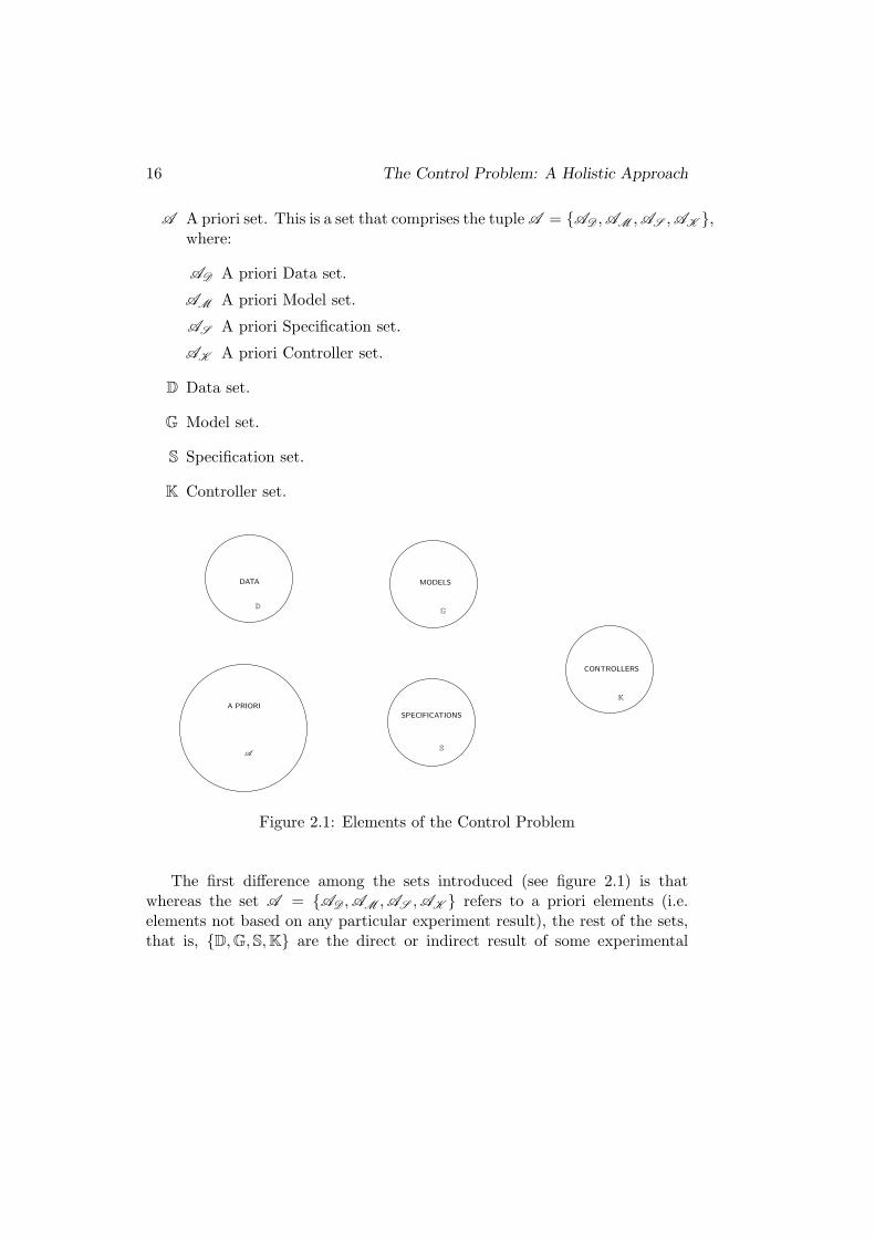
2.2 Elements of the Control Problem
We refer as the elements of the control problem the mathematical entitiesdefined and used through the control design process. We group these mathe-matical entities on the following sets:
16 The Control Problem: A Holistic Approach
A A priori set. This is a set that comprises the tuple A = AD , AM , AS , AK ,where:
AD A priori Data set.
AM A priori Model set.
AS A priori Specification set.
AK A priori Controller set.
D Data set.
G Model set.
S Specification set.
K Controller set.
DATA MODELS
SPECIFICATIONS
CONTROLLERS
A PRIORI
A
DG
S
K
Figure 2.1: Elements of the Control Problem
The first difference among the sets introduced (see figure 2.1) is thatwhereas the set A = AD , AM , AS , AK refers to a priori elements (i.e.elements not based on any particular experiment result), the rest of the sets,that is, D, G, S, K are the direct or indirect result of some experimental
Sec. 2.2. Elements of the Control Problem 17
data, thus being defined as a posteriori elements1. Consequently the a prioriset is the responsible of defining the whole mathematical structure in whichthe control problem is being tackled and possibly solved.
On the other hand, the a posteriori elements D, G, S, K are tangiblerealizations of the mathematical environment described by the a priori set.The a posteriori elements are divided in four sets in which the data set is theorigin of the rest of the sets, as in order to obtain any other a posteriori set,data is mandatory. The division of the sets follows the conceptual formulationof the control problem, that is, design a controller K for some given plant G
that fulfils some requirements S.
In the next paragraphs each set is described more thoroughly and we givesome examples of the assumptions normally taken over these sets.
A Priori Set
This set gathers all the a priori elements (i.e. elements that are not based ondata records). The a priori set is the responsible of defining the mathematicalstructure that will be assumed by the a posteriori elements of the controlproblem. In fact it is the a priori set which completely formalizes the controlproblem to be solved. Its importance is crucial, as the same problem, canbe either solvable or unsolvable regarding the a priori set. For example theproblem with the following elements: AS =Zero Stationary Error, AM =FirstOrder LTI Plant, AK =PD Controller, is not solvable, although changing thea priori set AK to be a PI Controller makes the solution achievable.
The a priori set is subdivided into four sets, AD , AM , AS and AK , re-garding the a priori considerations taken over the data , the model family, thespecifications considered and the controller to be designed. These sets are:
AD A priori Data set. This set defines the mathematical characterizationof the data. The related mathematical issues are defined from practicalaspects such as:
– Sensors number and placement.
1A priori elements are the elements provided by the control engineer. On the other handthe a posteriori elements are elements obtained through the analysis and manipulation ofcollected data.
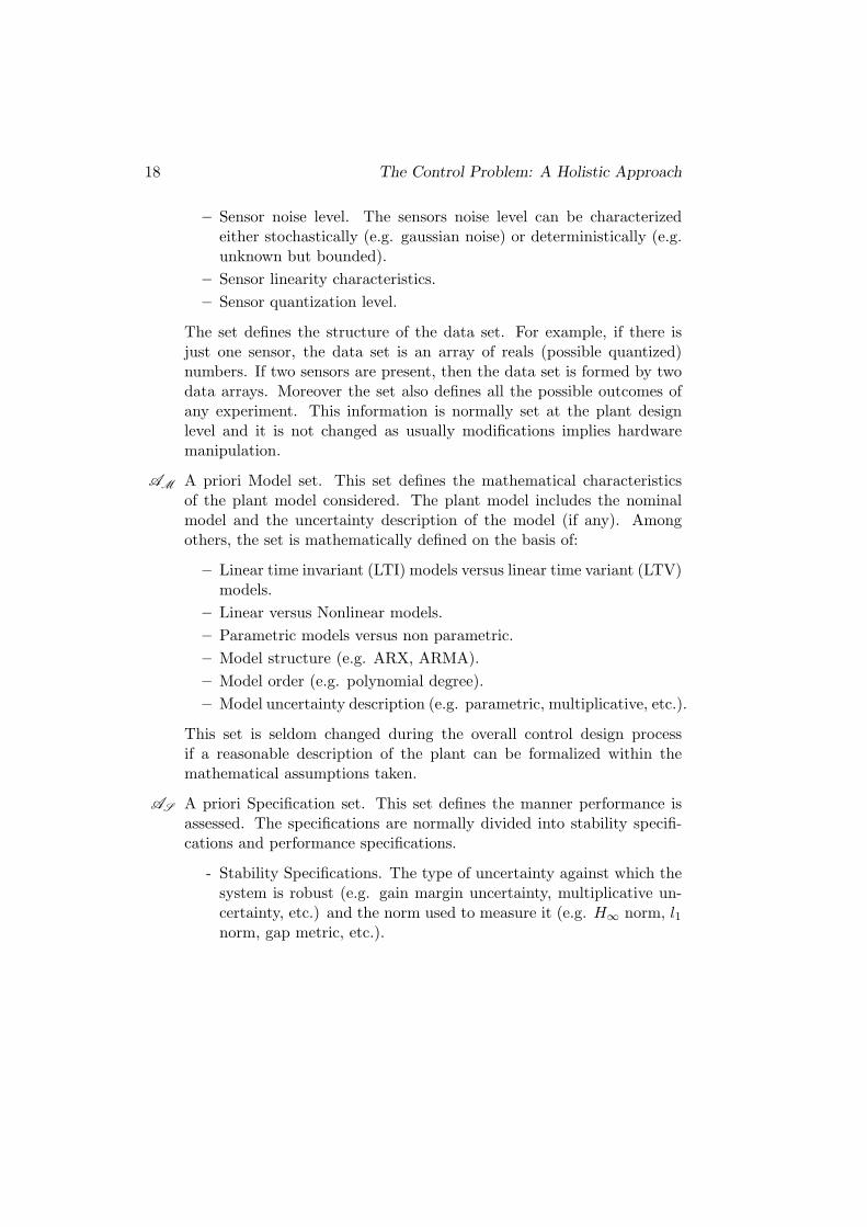
18 The Control Problem: A Holistic Approach
– Sensor noise level. The sensors noise level can be characterizedeither stochastically (e.g. gaussian noise) or deterministically (e.g.unknown but bounded).
– Sensor linearity characteristics.
– Sensor quantization level.
The set defines the structure of the data set. For example, if there isjust one sensor, the data set is an array of reals (possible quantized)numbers. If two sensors are present, then the data set is formed by twodata arrays. Moreover the set also defines all the possible outcomes ofany experiment. This information is normally set at the plant designlevel and it is not changed as usually modifications implies hardwaremanipulation.
AM A priori Model set. This set defines the mathematical characteristicsof the plant model considered. The plant model includes the nominalmodel and the uncertainty description of the model (if any). Amongothers, the set is mathematically defined on the basis of:
– Linear time invariant (LTI) models versus linear time variant (LTV)models.
– Linear versus Nonlinear models.
– Parametric models versus non parametric.
– Model structure (e.g. ARX, ARMA).
– Model order (e.g. polynomial degree).
– Model uncertainty description (e.g. parametric, multiplicative, etc.).
This set is seldom changed during the overall control design processif a reasonable description of the plant can be formalized within themathematical assumptions taken.
AS A priori Specification set. This set defines the manner performance isassessed. The specifications are normally divided into stability specifi-cations and performance specifications.
- Stability Specifications. The type of uncertainty against which thesystem is robust (e.g. gain margin uncertainty, multiplicative un-certainty, etc.) and the norm used to measure it (e.g. H∞ norm, l1norm, gap metric, etc.).
Sec. 2.2. Elements of the Control Problem 19
- Performance Specifications. The cost functions which measures theperformance (e.g. quadratic costs, etc).
AK A priori Controller set. This set establishes the mathematical definitionof the controller to be designed. The main considerations are:
- Controller Architecture (e.g. 1 D.O.F. Vs 2 D.O.F., Smith Predic-tor, cascade configuration, internal model control, etc).
- Controller Order and Structure (e.g. PI, PID).
The importance of this set is that it defines, in mathematical terms, thesearch space of the controller. If the solution to the control problem doesnot lie inside the search space, it never will be found. On the other handit can be the case that no solution exists hence the problem is unsolvablewhatsoever search space is chosen.
Data Set
The data set D comprises all the measured variables from one or more exper-iments. The data can come from an experiment, either in open loop or closedloop, or from normal plant operation. It is clear that D ⊂ AD , namely, theresult of any experiment (or experiments combination) must be a subset of theall possible experimental results given by the a priori data set. If the set D isempty (e.g. no experimental data) we are dealing only with a priori elements.All the a posteriori elements have their origin on this set.
Model Set
The model set G comprises the identified model family that are used to designa controller (a singleton if just a nominal model without error bounds is iden-tified). The model family is a subset of the model set defined in the a prioriinformation, thus G ⊂ AM . The set inclusion means that the model set is aparticularization, for some given data, of the a priori model set. The modelset is a posteriori set as data is mandatory to perform the identification. Anexample of the a priori model set is the set formed by first order plus time de-lay linear time invariant models (FOPTDLTI). On the other hand a posteriorimodel set is a FOPTDLTI with time constant τ = 5, gain k = 10 and delayd ∈ [0.5, 1].

20 The Control Problem: A Holistic Approach
Specification Set
The specification set S is the set containing the values and/or limits of thedesign specifications defined in the set AS . For example this set contains allthe specifications defined by a quadratic cost function which value is limitedby the amount α imposed by the designer. Again S ⊂ AS , thus this setis a particularization for some performance level. An example of stabilityspecification is the gain margin (e.g. a gain margin of 0.5).
Controller Set
The controller set K is the set of all controllers that accomplishes the specifica-tions defined in the above set S for all the plants on the model family G. Thesecontrollers are a subset of all the controllers defined in the a priori information(i.e. K ⊂ AK ). If no controller can be found to accomplish the requirementthen the controller set is empty, that is K = ∅. The most common a prioricontroller set AK is the PID controller. The controller set is then defined byall the values of KP , KI and KD which achieve the specifications.
2.3 Relationships Between Elements of the ControlProblem
The elements of the control problem already introduced are necessary to solvethe control problem but not sufficient. In fact some elements are the resultof manipulations and combinations of other elements. In this section we statethe relationships among the elements of the control problem in order to designa controller. First we identify each one of the element relations and definethe relationship on the basis of function theory. Secondly it is shown howeach one of these relationships can be related to areas of control theory (e.g.identification, control design, limitations in control, performance assessment,etc).
In figure 2.2 the elements are plotted together with their relationships.These relations are:
I Identification.
C Control Design.
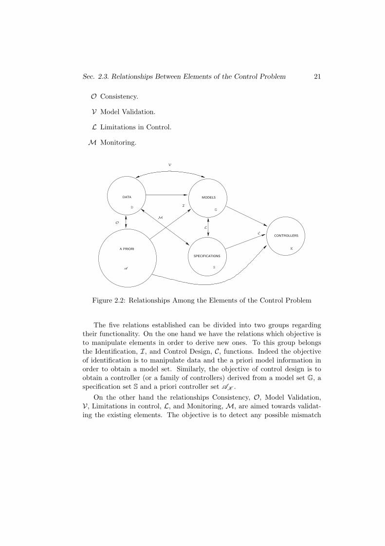
Sec. 2.3. Relationships Between Elements of the Control Problem 21
O Consistency.
V Model Validation.
L Limitations in Control.
M Monitoring.
DATA MODELS
SPECIFICATIONS
CONTROLLERS
A PRIORI
D
A
G
S
K
O
V
M
I
L
C
Figure 2.2: Relationships Among the Elements of the Control Problem
The five relations established can be divided into two groups regardingtheir functionality. On the one hand we have the relations which objective isto manipulate elements in order to derive new ones. To this group belongsthe Identification, I, and Control Design, C, functions. Indeed the objectiveof identification is to manipulate data and the a priori model information inorder to obtain a model set. Similarly, the objective of control design is toobtain a controller (or a family of controllers) derived from a model set G, aspecification set S and a priori controller set AK .
On the other hand the relationships Consistency, O, Model Validation,V, Limitations in control, L, and Monitoring, M, are aimed towards validat-ing the existing elements. The objective is to detect any possible mismatch
22 The Control Problem: A Holistic Approach
between the elements. The consistency check, O, is a validation of the col-lected data with the a priori data set. The Model Validation procedure, V,is aimed at finding invalidation results between the model set identified andthe experimental data collected. Similarly, the Monitoring relation M is avalidation between the specification set and the actual achieved specificationscalculated from collected data. Finally the Limitations in Control relation, L,is a consistency check between the established designer specifications and thelimitations imposed by the model set (e.g. right half plane zeroes and poles).
In the next paragraphs each relationship is established formally and de-scribed on the basis of well established control topics.
Identification
The aim of the identification is to derive a model (and possibly error bounds)for control design purposes. The identification is mathematically defined as anapplication from the set of possible models given by the a priori informationAM and the set of data D to the set of possible models AM .
Definition 2.3.1 The identification function I : AM xD → AM is defined as
I(g, d) = g ∈ AM |E(g) = d, ∀d ∈ Dwhere E(g) = d is any operator relating the a priori information to the data.(e.g. convolution operator y = G ∗ u).
♦
The topic of system identification has been of major importance for controlsystem design. The theory is well established and plenty of successful appli-cations, however recently (last 15 years) fundamental issues regarding identi-fication of models for controller design have modified the traditional point ofview (Gevers, 2006). The angular stone has been to consider the final use of themodel (e.g. prediction, control design) on the system identification process.Indeed, as it was pointed in (Skelton, 1989), small model-plant mismatches canlead to great different behaviors when both are operated in closed loop buttwo different systems can behave quite similarly under feedback. The reasonis that under feedback some model errors are amplified whereas other modelerrors are attenuated. Additionally, the concept of identifying the “real” planthas proven to be bogus (Hjalmarsson, 2005) due to the following reasons:
Sec. 2.3. Relationships Between Elements of the Control Problem 23
- The order of real systems is infinite.
- Data collected from plant are always finite.
- Data are always corrupted by noise.
The above considerations have directed intensive research in order to iden-tify “good” models for control design purposes. This research can be classifiedin two main points which are:
• Input experiment design. The fundamental importance of input exper-iment design for system identification has been pointed out in (Ljung,1999) (Soderstrom and Stoica, 1989). In (Bitmead et al., 1990) it isshown that under undermodelling conditions the identified plant dependson the input applied. Thus if a good model for control design purposesis pursued, the problem of input experiment design arises. This problemcan be tackled by identifying the plant in a closed loop setting. Theadvantage is that the same control loop weights the energy input that isapplied to the plant, thus providing more suited data for control designpurposes.
• Identification criterion. Once data is collected and a model structure ischosen, it remains to fit the parameters of the model with the experi-mental data. Several possibilities arise:
- Minimization of the discrepancy of a model and a plant. This is theapproach taken by classical open loop identification (Ljung, 1999).
- Minimization of the discrepancy of two controlled loops (Landauand Zito, 2006a).
- Minimization of the model-plant discrepancy measured through acontrol design cost function. This is the approach taken in iterativeidentification and control design schemes (Albertos and Sala, 2002).
The input experiment design and the identification criterion entwine to-gether arising the broader question of Open Loop Identification vs ClosedLoop Identification. The results mentioned above aims towards closed loopidentification, not to mention practical requirements such as identification ofunstable plants. Adaptation of classical prediction error methods to be ap-plied in closed loop settings can be found in (Landau and Zito, 2006a). The
24 The Control Problem: A Holistic Approach
model error obtained is weighted by a function depending on the closed loopsensitivity function S (e.g. S = (1+GH)−1), thus giving less error around thefrequencies of interest in which the S function is “big”.
Another completely different area of system identification that has cap-tured intensive research has been the identification of model error bounds,known also as robust identification or control oriented identification. The ori-gin of this topic lies on the requirements of robust control design procedures ofnot only a nominal model but also a model error bound. The robust identifi-cation problem was posed originally in (Helmicki et al., 1991) receiving consid-erably attention since then. Monographic publications are (Sanchez-Pena andSznaier, 1998) and (Chen and Gu, 2000). The approach taken was a worstcase deterministic approach, leading to controversial discussions between hardbounds and soft bounds. However after a decade of intensive research thereal limitation of the procedures proposed was established. The robust identi-fication methods where aimed towards identifying small uncertainty bounds,disregarding completely quality issues on the nominal model used to designthe controller. This together with their inherent conservativeness due to theworst case approach has limited its popularization.
Control Design
The cornerstone of the control problem lies on the controller design step. Infact the problem is solved if a proper controller is designed and implemented.The control design is mathematically defined as an application from a modelset G, a priori assumptions of the controller AK and the specification setS to a controller AK . It is expected that the designed controller performsaccordingly with the specifications for the whole family of models G.
Definition 2.3.2 The control design function C : GxSxAK → AK is definedas
C(g, s, k) = k ∈ AK |F (g, k) = s,∀g ∈ G,∀s ∈ Swhere F (g, k) = s states that the closed loop of g and k accomplishes theperformance requirements.
♦
Normally the knowledge on the plant is limited to certain levels of accu-racy and thus uncertainty is present. This arises the problem of robustness.
Sec. 2.3. Relationships Between Elements of the Control Problem 25
A controller is robust if certain property (either stability or performance) isaccomplished for all the members of certain family (Doyle et al., 1992). This isthe manner in which the robust control design approach tackles the problem ofuncertainty. First the plant is modelled as a family of plants in which lies thereal plant. Next, a robust controller is designed. As the resulting controller isrobust, the real plant is satisfactorily controlled2.
The above discussion allows us to classify model based control design ap-proaches in two main areas regarding the model characteristics considered:
• Classical design approaches. It comprises a wide range of different tech-niques. However their common point is the lack of model uncertaintyconsideraions during the design step.
• Robust design approach. In the 80’s a thorough investigation on ro-bustness issues started. The objective was to explicitly take into ac-count model uncertainty during the design step, which was found tobe the main drawback of the classical approach. In the seminal pa-pers (Zames, 1981) and (Doyle and Stein, 1981) the idea of robust controlis suggested. The robust design approach is presented in (Zhou, 1998)and (Sanchez-Pena and Sznaier, 1998).
Consistency
Consistency checks if the a priori information agrees with the experimentaldata and vice versa. In fact the consistency check can serve either to dis-regard wrong a priori information when proper data is used or to disregardexperimental procedures generating misleading data when truthful a prioriinformation is present.
Definition 2.3.3 We define the Consistency function O : A → AD as thefunction that returns all the possible data generated by the a priori set.
♦
2It is necessary to mention that although the robust control design procedures producerobust controllers, this fact does not mean that any other methods of controller design pro-duces non robust controllers. Indeed other control design methodologies can produce robustcontrollers too. The only difference is that the robustness requirement is not considered ex-plicitly in the design whereas robust control design takes robustness issues in consideration.
26 The Control Problem: A Holistic Approach
Definition 2.3.4 Given A , D and O, A and D are consistent if D ⊂ O(A )
♦
In words, the a priori set A and the a posteriori data set D are consistentif the data set is a subset of all the possible data generated accordingly withthe a priori assumptions.
The consistency issue is not a topic by itself in the control theory literature.However it can be related with fault tolerant control and fault detection is-sues. Fault tolerant control (Isermann, 1997) deals with the design of systemstolerant to faults (i.e. non allowed deviation of a characteristic or parameterof a system), leading to a system that can cope with faults. To this end, faultdetection (Blanke et al., 2003) is a mandatory step. The fault detection stepis a consistency check between current acquired data and a priori information.It should be noted however that fault detection includes changes on plant (e.g.time varying parameters). Thus plant variations are considered a type of fault.On the other hand the problem of plant variations can also be tackled froman identification point of view in the paragraph on model validation.
We expose the utility of consistency by means of a simple example.
Example 2.3.1 The a priori information about a SISO plant states that weare dealing with a first order system. However experimental data shows anoscillatory behavior of the output. Hence inconsistency is present.
Limitations
The fact that the implementation of a controller can change the dynamic be-havior of a system tends to mask the fundamental limitations of any physicalsystem (e.g. system power is limited, delays are unavoidable, etc.). A con-trol system can not be pushed further than its fundamental limitations (Seronet al., 1997). Control designs based on specifications aiming at higher per-formances than those allowed by the physical limitations are a certain fail-ure. Thus in order to avoid stating impossible designs, the compatibilitybetween the designer proposed specifications and the plant allowable speci-fications must be checked.

Sec. 2.3. Relationships Between Elements of the Control Problem 27
Definition 2.3.5 We define the Limitation function L : G → AS as thefunction that returns the allowable performance values imposed by the modelsfamily G.
♦
Definition 2.3.6 A control design problem based on the models family G isfeasible for some S if S ⊂ L(G)
♦
Thus the fundamental limitations requires that the set of desired specifi-cations is a subset of the achievable specifications.
Limitations on control literature appeared at the same time as control the-ory (see for example (Bode, 1945) (Horowitz, 1963)). The limitations are dueto plant structure (e.g. RHP poles and zeroes, delays) and actuator limita-tions (e.g. saturations, rate limitations, etc.). In (Skogestad and Postleth-waite, 1996) a good introduction to fundamental limitations is presented.
Model Validation
Once a model has been identified it remains to check its validity for the in-tended use. The term model validation is widely accepted although it is mis-leading. Admittedly, as stated in (Popper, 1958), the scientific method canonly invalidate existing theories. Thus a model can only be invalidated nevervalidated. This is so because further data could invalidate an existing vali-dated model by former data sets. In what follows the terms model validationand model invalidation will be used indistinctly, however a model can only beinvalidated.
There are certain identification algorithms that guarantees the identifiedplant is validated (e.g. interpolatory algorithms (Chen and Gu, 2000)). How-ever this is not the general case, hence the necessity of the validation step.
Definition 2.3.7 We define the Validation function V : G → AD as thefunction that returns all the possible data generated by the models family G.
♦
Definition 2.3.8 A models family G is validated against certain data set D
if D ⊂ V(G)
28 The Control Problem: A Holistic Approach
♦
In words a model is validated if the data at hand is a subset of all thepossible data that the model set can generate.
Model validation is highly related with the assumptions taken during themodel identification step, thus it is discussed in the bibliography of modelidentification. See (Ljung, 1999) (Soderstrom and Stoica, 1989) for validationof classical models and (Chen and Gu, 2000) for validation of robust identifiedmodels.
Monitoring
The final objective of a control system is to achieve certain performance speci-fications. If they are fulfilled then the problem is solved and no further actionsare needed. In order to assess performance a monitoring process over the datacoming from the controlled loop is necessary.
Definition 2.3.9 We define the Monitoring function M : D → AS as thefunction that returns the performance index measured from the data set D.
♦
Definition 2.3.10 A control system is under performance specifications S ifM(D) ⊂ S
♦
If the specifications calculated from data are a subset of the desired spec-ifications, the control system is performing as expected.
The monitoring process includes different issues. First the definition ofthe parameters in which the performance is based. In (Qin, 1998) (Harris etal., 1999) a review of performance monitoring techniques is presented. Theyare based on the comparison of the current performance with the performanceprovided by a minimum variance controller. On the other hand, once a param-eter for monitoring performance has been chosen, it is necessary to determineon the basis of the calculated parameter, if the system is under performance.This is not an easy task as normally we are dealing with variables defined onan stochastic framework. The use of hypothesis test and control charts havebeen presented as suited tools to manage the decision task. See for exam-ple (Balaguer and Vilanova, 2006c) (Balaguer and Vilanova, 2006d).
Sec. 2.4. Summary 29
2.4 Summary
In this chapter an abstract study of the control problem from a holistic pointof view has been conducted. The control problem has been divided betweenits elements and their relationships.
The elements have been divided in two subgroups regarding its dependencewith data. On the one hand the a priori elements which are fixed by thecontrol engineer and thus independent of future data. On the other hand dataare mandatory in order to obtain the a posteriori elements. The objectiveof the a priori elements is to set the mathematical framework in which theproblem is tackled and solved. On the contrary the a posteriori elements arethe formalization inside the abstract framework for some data set which givesa tangible solution.
Once the elements are established, it is possible to define their relation-ships. The relationships among the elements are classified through existingcontrol areas. Regarding the objective of the relationship it is possible toclassify the relationships between the ones that transform current elementsof the control problem into new ones and the ones which check consistencyamong these elements. It is worth nothing that any relation is an applicationrequiring both, a priori elements and a posteriori elements. This implies thenecessity of both elements in order to solve the problem.
As a result a framework is presented in which elements and relationshipsof the control problem which are normally hidden by the technicalities of thetechniques used, come to the surface. This is useful in several ways:
• First the scheme provides a framework in which compare distinct con-trol design approaches regarding the nature of the elements used, theirallowed modifications and relationships taken.
• Secondly the scheme helps to envisage new ways to manage the elementsand their relationships, helping in the design of new relations or addingnew features to existing relations (e.g. iterative control).
• Finally the proposed scheme is of interest in control education in orderto first establish the difference between the mathematical assumptionsand the real data and their importance in order to solve the control prob-lem. Secondly it presents the elements explicitly, stating the degrees of

30 The Control Problem: A Holistic Approach
freedom in any design. The framework also presents, in an organizedmanner, the existing control topics in a context that helps its presenta-tion, localization and understanding.
Chapter 3
Information and Control
The objective of this chapter is twofold, on the one hand to introduce the rela-tionship between information and control and on the other hand to define theinformation theory approach used to define the information theoretic frame-work for control design introduced in the next chapter.
First it is presented how the information concept entwines several aspectsof the control problem. In fact information is the basic concept on controltheory which arises at signal and at system level. The distinct aspects ofinformation on control theory are reviewed and finally the problem is focusedon the interplay of information on the procedure of designing a controller
Secondly distinct formalizations of information are presented. Informationis a term with different assumptions, definitions and meanings. We review theexisting scientific approaches to the concept of information and present theUncertainty Based Information theory as the one considered to formalize theproblem of designing high performance controllers.
31
32 Information and Control
3.1 Information and Control Theory
The relation between information and control systems is an important andcomplex issue. Admittedly the goal of any feedback control system is to gaincertainty on the system behavior under an uncertain environment by measur-ing some system variable. In (Newton et al., 1957) one of the characteristicsthat a feedback system must have is:
“(1), the action of the system on the output is determined, in part, by thevalue of the output”.
Additionally, regarding the justification of feedback, (Newton et al., 1957)states:
“The three major reasons for employing feedback control are: (1) Theprocess or actuator which supplies the output may have signal transmissioncharacteristics that make open-loop operation very difficult. (2) With feedbackthe precision of control can be made to depend largely upon the equipmentused to measure the output and to compare it with its ideal value. This factmay enable accurate control to be achieved in spite of inaccuracies and variablecharacteristics in the actuator or process. (3) The effect of disturbances onthe output may be suppressed by employing feedback, thereby obviating theneed to elaborate disturbance compensators that would be needed with openloop control.”
On the above discussions we can relate the term information (or its ab-sence) within different contexts. First feedback, in opposition to open loopschemes, requires extra information by measuring the output. Secondly, it isintroduced the “signal transmission characteristics”. This problem of charac-terizing the channel transmission characteristics was solved by the celebrated“A Mathematical Theory of Communication” (Shannon, 1948), which formedthe basis on information theory during nearly forty years. Finally it appearsthe problem of lack of information in the systems itself “inaccuracies and vari-able characteristics in the actuator or process” or uncertainty due to unknownsignals “effect of disturbances”. Hence we can conclude that first, the terminformation is in the very basis of control systems and, secondly, it is a conceptthat appears through distinct aspects such as, channel transmission, feedbacktheory and uncertainty on signals and systems.
Despite the fundamental importance of information on control systems,a complete information-theoretic framework for control systems is still lack-
Sec. 3.1. Information and Control Theory 33
ing (Zames, 1998) (Touchette and Lloyd, 2004).
Nonetheless information concepts have enriched control theory throughseveral well established control theories as Adaptive Control (Astrom and Wit-tenmark, 1989), Robust Control (Doyle et al., 1992), Fundamental Limitationsin Control (Skogestad and Postlethwaite, 1996) and Networked Control Sys-tems (Goodwin et al., 2006). A brief description of the relation of each theorywith information is presented.
• Adaptive Control. The main idea of adaptive control is to use the sensedoutput not only to calculate the control action but to modify the lawresponsible of calculating the control action. As a result informationcoming from the feedback is added to the controller itself, modifying itsparameters. This is accomplished by the recursive identification of theplant parameters and modifying the controller parameters either directlyor indirectly.
• Robust Control. The robust control paradigm was born as an answerto the problem of model uncertainty. In fact theoretical designs basedon existing controllers failed when experimentally tested due to modelerror issues. The goal of robust control is to relate by means of some un-certainty measure, the plant uncertainty with stability and performancespecifications. It is the first time that an information measure (e.g. ametric in H∞, l1, etc.) is used to establish a relation with either stabilityor performance margins.
• Fundamental Limitations in control. It is known that certain plant prop-erties impose limitations on the achievable performance by any con-troller. Structural aspects such as time delays, input saturations, righthalf plane (RHP) poles and RHP zeros impose limitations on the band-width. For example a RHP pole requires a minimum amount of band-width in order to stabilize a system. On the other hand, RHP zeros andtime delays impose a bound on the maximum bandwidth allowable. Theplant is experimentally impossible to control if the bandwidth requiredfor stabilization is greater than the allowable bandwidth of RHP zerosand delays. The fundamental limitations in control is a very importantaspect that, if not taken into account properly, can lead to stating controlproblems with no feasible solution.
34 Information and Control
• Networked Control Systems. Traditionally control theory has assumedthat controllers and plants communicate in an ideal manner. Howeverwith the technological developments of distributed control systems newissues relating communication and control has arisen. These issues arerelated with the effects of quantization and delays that exists in any realtransmission channel. In fact they are related with information ratestransmitted through the channels and the required information in orderto achieve certain performance level.
The above information and control topics can be classified in two maingroups. Firstly techniques that deal with information deficiencies at the plantlevel. Secondly topics that study transmission of information on the controlproblem. Adaptive control and robust control belong to the first group. Infact both are techniques to cope with uncertainty, although the solution theyprovide to the problem of lack of information is of different nature. On theone hand adaptive control tries to continuously capture information in orderto reduce uncertainty. On the other hand, robust control tries to measure un-certainty and relate it with the pursued objective, in order to design a properlycontroller. Conversely fundamental limitations in control and networked con-trol systems deal with information transmission at the signal level and howthe limitations affects the overall performance.
On the rest of this thesis we focus on information concepts related withplant uncertainty, hence related to the adaptive and the robust control paradigm.Consequently the information-theoretic approach is aimed towards studyingthe information flow for control design purposes covering classical issues asmodel identification and controller design plus additional issues as informationmonitoring, fundamental limitations in control, model validation and consis-tency of a priori information. Our problem is how to manage informationsources to design high performance controllers.
Summing up the concepts presented in this section are:
• Information plays a fundamental role in control theory.
• Information, as far as control theory is concerned, is a multiple con-cept. For example the information rate transmitted through the feed-back channel, the lack of information (i.e. uncertainty) of a model, etc.
• We focus on information for designing high performing controllers.
Sec. 3.2. What Is Information? 35
• The main point that aims our study is that of adding new informationand that the new information produces beneficial results.
3.2 What Is Information?
The concept of Information is a broad and elusive one. It is used for a widevariety of meanings and formalized within distinct theories. The objective ofthis section is first to review the existing scientific approaches to the conceptof information and secondly to establish the meaning of the term informationthat is being used throughout this thesis.
The concept of information has been investigated under distinct concep-tual frameworks as Computational Complexity (Kolmogorov, 1965) (Chaitin,1987), Uncertainty Based Information (Klir and Wierman, 1999) (Klir, 2006),Logic (Devlin, 1991) and Systems Organization (Stonier, 1990). For each oneof the proposed theories, information is defined in distinct terms. For exam-ple the computational complexity paradigm measures the information of anobject by the length of the shortest possible program to define the object. Onthe other hand, uncertainty based information measures information as thecapacity of reducing uncertainty whereas the systems organization approachto information views information as a property to organize a system.
In what follows we focus on Uncertainty Based Information as this is theconceptualization of information adopted in this thesis. Uncertainty BasedInformation theory considers uncertainty as a result of some information de-ficiency. Consequently certain amount of information can reduce uncertainty,thus implying that the amount of information gained can be measured by thereduction of uncertainty. Inside this framework uncertainty and informationhave an inverse relationship, thus
Information = Uncertainty−1 (3.1)
The Uncertainty Based Information theory presented can be formalizedunder several mathematical frameworks. One of the main results of the Un-certainty Based Information Theory has been to establish the multidimension-ality of the uncertainty concept. In fact, distinct types of uncertainty exists.For example, under classical set theory, uncertainty is related with the size(number of elements) of a set. On the other hand, the mathematical theory of
36 Information and Control
communication, which is also an uncertainty based information theory, char-acterizes uncertainty on the basis of probability theory. Thus uncertainty canhave a very different nature.
We formalize uncertainty on the basis of Classical Set theory. Thus uncer-tainty is related with the set’s size. The bigger the set the more uncertain.This type of uncertainty is referred as nonspecificity (Klir and Wierman, 1999).Notwithstanding, in the information theoretic framework presented in the nextchapter the information of some sets follows an inverse relation, that is thebigger the set the more informative the set. The rationale behind this choicewill be clear in the next chapter, however consider that, as far as the a priorimodel set is considered, the bigger the set (e.g. the higher model order) themore informative the a priori model set (e.g. more representation capacity).The main idea is that information is measured through a set size.
The increase of information (reduction of uncertainty) is pursued for thebenefit it can provide. In fact it is debatable that a more detailed model ismore informative, for control design purposes, if it does not help to improvethe designed performance controller. This arise the distinction between theterms Information and Information Value. As defined in (Sheridan, 1995), theterm Information refers to the reduction of uncertainty whereas InformationValue refers to what can be gained by the uncertainty reduction. Thus theconcepts of Information and Relevant Information can be defined as:
Information = Reduction of Uncertainty (3.2)
Relevant Information = Information that Improves Performance (3.3)
We analyze the general control problem on the basis of existing informationtheory (i.e. Uncertainty Based Information theory) and arise the question ofhow information should be managed inside the uncertainty based frameworkin order to achieve high performance controllers.
The interplay of uncertainty and control systems is normally viewed asa negative unavoidable limitation. Indeed uncertainty is the result of someinformation deficiency. In control problems information deficiencies can arisedue to:
Sec. 3.2. What Is Information? 37
• Incompleteness. The information at hand to solve the control problemis always incomplete. For instance, data are always finite, data containsome frequency components whereas other frequency ranges must beabsent.
• Imprecision. Imprecision of information is another difficulty. For exam-ple data is normally corrupted by noise. As a result, even the informa-tion is complete (e.g. the whole frequencies of interest are captured),this information is imprecise.
• Contradiction. This lack of information is of special interest in the con-trol problem as it is a warning of inconsistency (e.g. a model that isnot validate). This can be a sign that the mathematical machinery is oflimited capacity in order to capture the complexity of the problem.
These facts can limit the achievable performance of the control system1.
Nonetheless uncertainty also plays a beneficial role on the control designproblem. The positive aspect is due to complexity issues. Although it wouldbe possible to obtain models which are a perfect representations of realitythe mathematical framework required to manage these models would be toocomplex to be useful. It is possible to reduce the problem complexity byincreasing the problem uncertainty (e.g. modelling a nonlinear plant as a linersystem plus additive uncertainty). Thus it can be concluded that uncertaintyis a two faced coin. Uncertainty can limit the achievable performance but,at the same time, uncertainty can transform complex problems into tractableones.
To sum up the term information used throughout this thesis means in-formation on the sense of Uncertainty-Information Theory, with the followingproperties:
• Classical Set theory description of uncertainty.
• Information = Uncertainty−1
1It is not sure that the limits of performance of a control system are a consequence ofplant uncertainty. It could be possible that the limitations on the control design followtheir fundamental limitations. In that case it is arguable that a reduction of uncertaintycould improve the performance. As an example imagine a first order plant with a delay of10 minutes and a time constant of one second. Which is the benefit of reducing the timeconstant uncertainty by 1% on the overall performance?

38 Information and Control
• Information for control design purposes.
Chapter 4
Information Characterizationof the Control Problem
In this chapter we endow the framework of the general control problem with theinformation measure by using the Uncertainty based Information theory. Theapproach gives insight on two important aspects for control design. First wedetermine exhaustively the information sources available to accomplish a suc-cessful control design. Secondly we study the relations between the informationelements by deriving inclusion relations that must be fulfilled in order to assurean information increase. It is shown however that the inclusion relations arenot sufficient and other aspects must be considered
39
40 Information Characterization of the Control Problem
4.1 Introduction
In Chapter 2, a framework to analyze the model based control problem hasbeen present. The framework is divided in elements and relationships amongthese elements.
In the present chapter our aim is to endow the cited elements and relationswith an information measure. To this end, the Uncertainty Information The-ory is used to define the information capability of the elements and relations.The information definition hinges on the two main goals of the model basedcontrol problem. On the one hand to derive the smallest possible model set, asthe smaller the model set the more informative the set. On the other hand, todesign a controller. In this case the bigger the controller set the better. Thisfact is trivial in the case of the solvability of the control problem. In fact, ifthe problem is solvable the controller set has at lest one element: the designedcontroller. Conversely if the problem is not solvable the controller set is empty.Moreover, the “bigger” the controller set can imply benefits from a controllerrobustness point of view (i.e. robustness properties on the control loop due tocontroller uncertainty). For example imagine that the proportional controllerthat solves the control problem is the one with the gain value equal to K0, andthat any deviation for this value violates the specifications. From a practicalpoint of view the problem is not solvable. On the other hand if the controllerset is defined by a gain comprised between [Kmin, Kmax], the controller is morelikely to be solvable1.
The benefits of characterizing the elements and relations with an informa-tion measure are:
• First we are able to enumerate all the possible information sources fromwhich the control problem can beneficiate. We can classify the informa-tion sources in three groups regarding their nature. These are:
– Data Set: Information coming from experimental data.
– A Priori Set: Mathematical framework in which the control problemis posed.
1This discussion has nothing to do with the fact that the design algorithm returns just asingle controller. We mean the set of all controllers that solve the control problem, regardlessthe ability to find any of them. Therefore this is related to the sensibility of the solutionwith respect to the problem posed.
Sec. 4.2. Information and Identification 41
– Algorithms: Transformations of the elements (e.g. identification).
• Once an information measure is provided, it is possible to analyze therelations among the elements. Necessary conditions over the elementsfor information increase are stated. Moreover it is seen that to obtainalso sufficiency conditions, the algorithms for identification and controldesign must possess certain properties.
4.2 Information and Identification
The goal of system identification could be understood, from a naive point ofview, as identifying a mathematical model that represents the plant perfectly.This is however neither possible nor desirable. It is not possible due to fun-damental limitations (e.g. signal to noise ratio, finite number of samples).It is not desirable because model complexity must be kept tractable to meetthe level of current control design algorithms (e.g. LTI) when identifying realplants (e.g. non-lineal, time varying, infinite order).
Notwithstanding the identified model must capture the behavior of thereal plant within some accuracy degree. This is accomplished by identifyingnot a nominal model but a family of models, that is a model set. For controldesign purposes, it is desirable that the model set be as fitted as possible. Inthe limit case the model set would consist in just one model, the real plant.
Following the Uncertainty Based Information theory we define the infor-mation relation between model sets as follows:
Definition 4.2.1 A model set Gi is more informative than Gj if and only if(iff)
Gi ⊂ Gj and Gi 6= ∅♦
In words, the definition states that the lesser the elements of a model set themore informative the set. Additionally the set must consist of at least oneelement apart from the empty element (i.e. must be distinct than the emptyset).
Recalling the definition of identification (i.e. I : AM xD → AM ), theincrease of information on the model set can be pursued by modifying thefollowing variables:
42 Information Characterization of the Control Problem
• The identification algorithm, I.
• The data set, D.
• The a priori model set, AM .
The first variable, the identification algorithm, is a relationship of theelements of the control problem whereas the other two variables, the dataset and the a priori model set, are elements of the control problem. In whatfollows, we analyze the mentioned variables and their properties in order toincrease the information on the model set.
4.2.1 Identification Algorithm
For the sake of readability it is worth to remind that the result of the identifi-cation algorithm is a model set, so we can write the following equality relation,G = I(D, AM ).
Definition 4.2.2 For a given data set D and a priori model set AM , theidentification algorithm Ii is more informative than the algorithm Ij iff
Ii(D, AM ) ⊂ Ij(D, AM )
andIi(D, AM ) 6= ∅
♦
Definition 4.2.2 states that, for the same domain (i.e. elements D and AM )if the model set resulting from algorithm Ii is smaller than the one resultingfrom algorithm Ij , then the algorithm Ii is more informative than algorithmIj . It can be said that the algorithm that makes a better use of the sameoriginal information providing a smaller model set is more informative.
We however do not pursue longer in this thesis the possibility of gaininginformation through the identification algorithm. The main reason is thatexisting algorithms normally give the smallest possible set achievable with thecurrent data and a priori model set assumptions, as they are formulated on thebasis of some optimal problem, so no advantage can be foreseen by modifyingthe algorithm. Moreover the identification algorithm is very dependent onthe a priori assumptions on the model set and data set. As a result the
Sec. 4.2. Information and Identification 43
modification of the identification algorithm normally implies the modificationof other elements (e.g. a priori model set, a priori data set, etc.) which canbe not desirable.
4.2.2 Data Set
Definition 4.2.3 For a given algorithm I and a priori model set AM , thedata set Di is more informative than the data set Dj iff
I(Di, AM ) ⊂ I(Dj , AM )
andI(Di, AM ) 6= ∅
♦
It should be noted that the measure of information content of a data set isperformed through the identification algorithm and keeping the a priori modelset constant. Under this framework, the more informative data are the datathat provides the smallest model set.
A necessary condition for a data set Di to be more informative than thedata set Dj , is that the data set Dj must be included in the data set Di,namely the more informative the data set, the “bigger” the data set (e.g.more samples, more experiments, etc).
Theorem 4.2.1 If I(Di, AM ) ⊂ I(Dj , AM ) then Dj ⊂ Di
Proof: First of all assume that the data set D can be divided in distinct setsindexed by n (e.g. the index n can be the experiment number or the samplenumber). Given the data set D the smallest model set obtainable is given bythe intersection of all the identifications performed with the given data set (e.g.the intersection of all the models identified with the experiments belonging toD), that is G =
⋂Nn=0 I(Dn, AM ).
Given the data set Dj , assume that the optimal model set obtained is Gjo
which by the above discussion it turns out to be equal to⋂Ni
n=0 I(Dn, AM ).
If a new data set Di provides a better model set Gio that is
Gio ⊂ Gjo
44 Information Characterization of the Control Problem
This implies thatDi⋂
n=0
I(Dn, AM ) ⊂Dj⋂
n=0
I(Dn, AM )
The inclusion operator means that the left hand side must content more setintersections in order to be smaller, then
Dj⋂
n=0
I(Dn, AM )
Di⋂
m=Dj+1
I(Dm, AM ) ⊂Dj⋂
n=0
I(Dn, AM )
As a result the set Di contains elements that do not belong to the set Dj
thus
Dj ⊂ Di
Example 4.2.1 In this example we consider the well known Least SquaresIdentification Method (LSM) which is a particular case of the Prediction Er-ror Identification framework (Ljung, 1999). The method is based on findingthe parameter vector θ of the model y(t|θ) = G(θ)u(t) which minimizes theprediction error ǫ(t, θ) = y(t)− y(t|θ). This is accomplished by minimizing thefunction
VN (θ) =1
N
N∑
t=1
ǫ2(t, θ) (4.1)
where N is the number of data samples. It can be proven that, asymptotically(no bias error), the parameters converge to the optimum limit θ∗.
We consider the parameter error variable given by θN − θ∗, it turns out tobe a normally distributed variable N(0, 1
N P ). Thus the standard deviation of
the error variable θN − θ∗ is proportional to the 1√N
, that is θN − θ∗ ∝ 1√N
.
Thus it follows that if we have a data sets D1 with N1 samples then the estimateθN1
− θ∗ ∝ 1√N1
. If we want a smaller parameter variation, that is a smaller
parameter set it follows that θN2− θ∗ ∝ 1√
N2, thus N2 must be bigger than N1.
Sec. 4.2. Information and Identification 45
However the condition of Dj ⊂ Di is not sufficient to guarantee the increaseof information as it depends on the algorithm and data properties. This factconducts us to the following theorem that is proven false by means of a coun-terexample.
Theorem 4.2.2 The converse of theorem 4.2.1, that is
Dj ⊂ Di −→ I(Di, AM ) ⊂ I(Dj , AM )
is, in general, not true.
Proof: The condition of data set increase is not sufficient for a model familyreduction mainly for two reasons. First the algorithm must make use of theextra data. Secondly the extra data can contain data coming from a failuresituation (e.g. plant variations, sensor and/or actuator failures, etc) or beingnot persistently exciting data, then although the new data set contains datathat does not belong to the former data set, the data is not helpful in orderto reduce the model set.
Example 4.2.2 Assume that the model to be identified is a straight line (i.e.y = m ∗ x + b). The data set consists of coordinate pais (i.e. (xi, yi), fori = 1..N). The proposed algorithm takes the first sample (x1, y1) and secondsample (x2, y2) and calculates the parameters m and b by solving the linearequations system, that is:
∣
∣
∣
∣
mb
∣
∣
∣
∣
=
∣
∣
∣
∣
x1 1x2 1
∣
∣
∣
∣
−1 ∣
∣
∣
∣
y1
y2
∣
∣
∣
∣
The identification is solvable whenever the number of data samples N isequal or bigger than 2. However although we take more samples, the new ac-quired information is not used by the algorithm. It follows that an increase onthe data set does not imply an increase on model information. The limitationlies on the capability of the identification algorithm in making use of the ex-tended data set. In fact the algorithm not even provides an error measure ofthe estimates.
46 Information Characterization of the Control Problem
Example 4.2.3 Consider a static system which gain K1 is to be identified.The samples are measured with a sensor affected by Gaussian noise N(0,σ2).As a result the identified gain K1 is also a Gaussian variable with distributionN(K1,σ
2).
Now assume that the system gain is not time invariant and that at sometime instant “tk” the system gain abruptly changes its value to K2 and moredata samples are acquired so the data set increases. However the data set isnow composed by two distinct random variables, K1 and K2. If the gain is nowestimated from this “bigger” set, Kest equals the sum of two random variables,K1 and K2, hence the distribution of Kest results to be N(K1 + K2,2σ2). As aresult, not only the size of model set has increased by a factor of two (e.g. 2σ2)but also we can not guarantee that the real gain value belongs to the model set.
This example shows the necessity of using proper data for the identificationprocedure. That means to use data free of failures of any kind.
Summarizing, a necessary condition for increasing the model set informa-tion is that of increasing the data set. On the other hand an increase of thedata set does not necessarily mean the increase of model set information. Thereason is that the algorithm must be able to take advantage of the new in-corporated data and that the new data must be generated under no failuresituations.
4.2.3 A Priori Model Set
Definition 4.2.4 For a given algorithm I and data set D, the a priori modelset AM i is more informative than the a priori model set AM j iff
I(D, AM i) ⊂ I(D, AM j)
andI(D, AM i) 6= ∅
♦
Again, the measure of information content of the a priori model set is per-formed through the identification algorithm and keeping the other parametersconstant. Under this framework, the more informative a priori model set isthe one that provides the smallest model set.
Sec. 4.2. Information and Identification 47
A necessary condition for a priori model set AM i to be more informativethan the a priori model set AM j , is that the a priori model set AM j must beincluded in the a priori model set AM i, namely the more informative the apriori model set, the “bigger” (in terms of elements) the a priori model set.
Theorem 4.2.3 If I(D, AM i) ⊂ I(D, AM j) then AM j ⊂ AM i
Proof: (by contradiction). Assume that AM i ⊆ AM j . By hypothesis weknow that I(D, AM i) ⊂ I(D, AM j), which for short we can write as Gi ⊂ Gj .
If AM i = AM j implies that Gi = Gj which is a contradiction.
Consider now that AM i ⊂ AM j and that the optimum a priori model set(i.e. the one that produces the smallest model set) AM o belongs to AM i,that is AM o ∈ AM i. This however implies also that AM o ∈ AM j which is acontradiction with the assumption of the model set Gi being optimal. Thus
AM j ⊂ AM i
However the condition AM j ⊂ AM i is not sufficient to guarantee the in-crease of information as it again depends on the algorithm characteristics.This fact conducts us to the following theorem.
Theorem 4.2.4 The converse of theorem 4.2.3, that is
AM j ⊂ AM i −→ I(D, AM i) ⊂ I(D, AM j)
is, in general, not true.
Proof: Think, for example in the trade-off of bias-variance error on theidentification prediction error method (Ljung, 1999). If the model is overpa-rameterized the model set increases due to variance errors.
48 Information Characterization of the Control Problem
In this section we have studied the influence of the a priori model set onthe model set information. We can understand the a priori model set as amathematical capacity of representation. A necessary condition for increasingthe information of the model set is increasing the a priori model set, that isincreasing the capacity of representation. On the other hand an increase ofthe a priori model set does not necessarily mean an increase of model set infor-mation as the problem of parsimony can limit the benefits of increasing the apriori model set if there is already enough degree of freedom to mathematicallycapture the plant.
4.3 Information and Control Design
The objective of the control design is to provide a controller or a family ofcontrollers, defined by the controller set K, that achieves the specificationslevel defined by the set S over the whole model set G. The controller set K
is normally a singleton (i.e. a unique controller) as it is implemented onlyone controller. However the controller set size is somehow related with con-troller robustness issues (that is tolerance to controller implementations im-precisions). Qualitatively, the more robust the controller (in the sense of con-troller uncertainty), the bigger the controller set. Thus the control problem issolvable whenever K 6= ∅.
Definition 4.3.1 A controller set Ki is more informative than Kj iff
Kj ⊂ Ki
♦
Definition1 4.3.1 introduces the informativeness concept of a controller setK by the set size. We pursue the biggest controller set as possible. Firstbecause this implies solvability of the problem and secondly, as discussed, dueto robustness issues. We can conclude that for a given control problem, thegreater the number of controllers that solve the problem the better.
Recalling the definition of control design (i.e. C : GxSxAK → AK ), theinformation increase of the controller set can be pursued by modifying thefollowing variables:
• The control design algorithm, C.
Sec. 4.3. Information and Control Design 49
• The model set, G.
• The specifications set, S.
• The a priori controller set, AK .
The first variable, the identification algorithm, is a relationship of theelements of the control problem whereas the other three variables, the modelset, the specification set and the a priori controller set are elements of thecontrol problem. We analyze these variables and their properties in order toincrease the size of the controller set.
4.3.1 Control Design Algorithm
The result of the control design algorithm is the controller set so we can writethe following equality relation, K = C : GxSxAK → AK .
Definition 4.3.2 For a given model set G, specifications set S and a prioricontroller set AK , the control design algorithm Ci is more informative thanthe algorithm Cj iff
Cj(G, S, AK ) ⊂ Ci(G, S, AK )
♦
Definition 4.3.2 states that, for the same domain (i.e. elements G, S andAK ) if the controller set resulting from algorithm Ci is bigger than the oneresulting from algorithm Cj then the algorithm Ci is more informative than Cj .It can be said that the algorithm that make a better use of the same originalinformation providing a bigger controller set is more informative.
We however do not pursue longer in this thesis the possibility of design-ing a bigger controller set through the design algorithm as normally designalgorithms just return one controller (i.e. a singleton), thus Definition 4.3.2.
4.3.2 Model Set
Definition 4.3.3 For a given design algorithm C, a specifications set S and apriori controller set AK , the model set Gi is more informative than the modelset Gj iff
C(Gj , S, AK ) ⊂ C(Gi, S, AK )

50 Information Characterization of the Control Problem
♦
It should be noted that the measure of information content of a model setis performed through the control design algorithm and keeping the domainconstant (i.e. C, S and AK ). In words, the most informative model set is theone that provides the biggest controller set.
A necessary consequence for a model set Gi to be more informative thanthe model set Gj , from a control design point of view, is that the model setGi must be included in the model set Gj , namely the more informative themodel set, the “smaller” (in terms of elements) the model set, which agreeswith Definition 4.2.1.
Theorem 4.3.1 If C(Gj , S, AK ) ⊂ C(Gi, S, AK ) then Gi ⊂ Gj
Proof: (by contradiction) By hypothesis C(Gj , S, AK ) ⊂ C(Gi, S, AK ),which for short let rewrite as Kj ⊂ Ki. The set K is the set of all controllerswhich achieve the specifications level S over all the model family G. Assumethat Gj ⊆ Gi.
If Gj = Gi that implies Kj = Ki, a contradiction.
If Gj ⊂ Gi, all the controllers Ki achieve S not only over Gi but also Gj .Then it follows that Kj ⊂ Ki what is a contradiction, thus
Gi ⊂ Gj
However the condition of Gi ⊂ Gj is not sufficient to guarantee the increaseof controller set information as it depends on the algorithm characteristics andthe relevancy of model set to the control design purposes. This fact conductsus to the following theorem:
Theorem 4.3.2 The converse of theorem 4.3.1, that is
Gi ⊂ Gj −→ C(Gj , S, AK ) ⊂ C(Gi, S, AK )
is, in general, not true.
Sec. 4.3. Information and Control Design 51
Proof: The decrease of models could be irrelevant from a control point ofview (i.e. easy to control models, not limiting achievable performance).
As a conclusion a necessary property for an increase of the controller setis a decrease of the model set. However a model set reduction is not sufficientto guarantee the increase on the controller set.
4.3.3 Specification Set
We define the information content of the specifications set S in the same waythat the information content of the model set G.
Definition 4.3.4 The specification set Si is more informative than the spec-ification set Sj iff
Si ⊂ Sj
♦
The rationale behind this definition is that, the smaller the specificationsset the higher the performance level, as other lower performance levels arerejected and thus not included in the new specifications set. Normally thisset is fixed by the designer. However, regarding the information content onthe whole control problem, the specifications set could be managed as a newcontrol variable. The information of the specification set could be understoodas an information level required in order to solve the control problem.
The relations between controller set information and the specifications setinformation is given by the following two theorems.
Theorem 4.3.3 If C(G, Si, AK ) ⊂ C(G, Sj , AK ) then Si ⊂ Sj
In words, if the controller set diminishes then the specifications level in-crease.
Proof: (by contradiction). Assume that C(G, Si, AK ) ⊂ C(G, Sj , AK ), forshort, Ki ⊂ Kj . Assume also that Sj ⊆ Si.
If Sj = Si then Ki = Kj , a contradiction.
52 Information Characterization of the Control Problem
If Sj ⊂ Si that would imply that Kj gives better performance that Ki,which is a contradiction with the assumption that Ki ⊂ Kj , thus
Si ⊂ Sj
However the condition of Si ⊂ Sj is not sufficient to guarantee the decreaseof controller set information as it depends on the relevancy of model set forcontrol design purposes. This fact conducts us to the following theorem.
Theorem 4.3.4 The converse of theorem 4.3.3, that is
Si ⊂ Sj −→ C(G, Si, AK ) ⊂ C(G, Sj , AK )
is, in general, not true.
Proof: The condition it is not sufficient as the increase of performancedemanded could be provided by the whole existing controller set.
4.3.4 A Priori Controller Set
Definition 4.3.5 For a given algorithm C, model set G and specificationsset S, the a priori controller set AK i is more informative than the a prioricontroller set AK j iff
C(G, S, AK j) ⊂ C(G, S, AK i)
.♦
Measuring again the information content through the control design algo-rithm, the more informative a priori controller set is the one that provides thebiggest controller set.
A necessary condition for a priori controller set AK i to be more informativethan the a priori model set AM j , is that the a priori model set AM j must beincluded in the a priori model set AM i, namely the more informative the apriori controller set, the “bigger” (in terms of elements) the a priori controllerset.
Sec. 4.4. Summary 53
Theorem 4.3.5 If C(G, S, AK i) ⊂ C(G, S, AK j) then AK i ⊂ AK j
Proof: (by contradiction). Assume that C(G, S, AK i) ⊂ C(G, S, AK j), forshort, Ki ⊂ Kj . Assume also that AK j ⊆ AK i.
If AK j = AK i then Ki = Kj , a contradiction.
If AK j ⊂ AK i that would imply that AK i has more representation ca-pacity than AK j , which is a contradiction with the assumption that Ki ⊂ Kj ,thus
AK i ⊂ AK j
However the condition of AK i ⊂ AK j is not sufficient to guarantee theincrease of information as it again depends on the algorithm characteristics.This fact conducts us to the following theorem.
Theorem 4.3.6 The converse of theorem 4.3.5, that is
AK i ⊂ AK j −→ C(G, S, AK i) ⊂ C(G, S, AK j)
is, in general, not true.
Proof: The condition is no sufficient as the extra representation capacityand secondly the extra representation capacity could not be useful for findinga better controller set. For example a PID controller does not offer advantagesover a PI if we are only interested in steady state error.
4.4 Summary
In this chapter we have seen the possible sources of information available tothe control problem and the relations of these information elements in orderto obtain better performing control systems.
We have seen that it is possible to reduce the models family by increasingthe data set and the a priori model set. Of course the identification algorithm
54 Information Characterization of the Control Problem
should make use of the extra information in order to be the goal achievable.Moreover the new data should be free of failures of any type.
Regarding the controller design, we have seen that the bigger the controllerset that achieve the required specifications over a model set the better. It ispossible to increase the controller set by diminishing the model set and byincreasing the mathematical representation of the a priori controller set. Thespecifications set is a designer variable. However if the controller set diminishesthe specification level increases.
On the contrary a sufficiency condition for uncertainty reduction mustcome from increasing the sets and taking advantage of the new informationby means of algorithm capabilities. In table 4.4 we present a summary of theinformation sources of the control problem and the necessity conditions forinformation increase of the element sets.
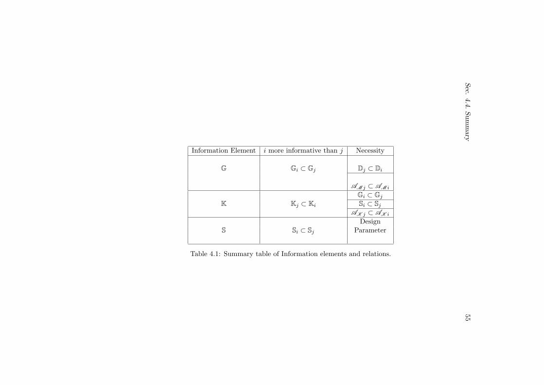
Sec.
4.4.Sum
mary
55
Information Element i more informative than j Necessity
G Gi ⊂ Gj Dj ⊂ Di
AM j ⊂ AM i
Gi ⊂ Gj
K Kj ⊂ Ki Si ⊂ Sj
AK j ⊂ AK i
DesignS Si ⊂ Sj Parameter
Table 4.1: Summary table of Information elements and relations.

56 Information Characterization of the Control Problem
Chapter 5
Information Supervision ofAdaptive Control Schemes
In this chapter the information framework presented in the previous chapter isused for analyzing existing adaptive control schemes. The objective is to studythe information flow of adaptive schemes in order to compare and discussproblems and solutions of the approaches. The chapter covers the followingsections:
• First the term supervisor is defined as an entity that manages the infor-mation flow in order to accomplish some goal.
• The existing adaptive control definitions are reviewed from literature anda new definition that comprises all the particularities of the adaptivecontrol term is established.
• Two adaptive control procedures, the “Model Reference Adaptive control”and the “Windsurfer approach” to iterative control, are analyzed regard-ing their information flow management. The comparison is accomplishedunder the information framework proposed in Chapter 4. Thus, it ispossible to compare the approaches and to relate well know problems andpossible improvements with the way information is managed.
57
58 Information Supervision of Adaptive Control Schemes
5.1 Information Flow Management: Supervisors
In Chapter 2, the control problem has been defined on the basis of its consti-tutive elements and relationships. Additionally the scheme has been endowedwith an information measure that allows to establish and analyze informationrelations among the elements. However the conceived framework is a static onein the sense that no indications are given on how to process the information.
In fact the control design problem is a problem of managing the informationflow. For example, first data is acquired and on the basis of some a priori modelset, a nominal model is identified. Hence with the identified model a controlleris designed and a solution proposed. The following considerations are in use:
• First we can identify an information flow. The first step is to acquiredata and the controller is designed after a model is identified. There isa causality relation between information elements.
• The information relations considered are a designer choice. For exam-ple on the previous example there are no considerations about modelvalidation, model uncertainty bounds, fundamental limitations, etc.
• The steps can be repeated and/or modified. Accordingly, even if thesame actions are taken into account, the same process can be repeatedseveral times (e.g. adaptive control) producing a distinct informationflow management.
• Information can be stored for further use or just disregarded.
As a result of the above considerations, it is clear that the control designproblem is a process in which the information elements stated in the frameworkof Chapter 4 must be managed in some way, resulting in an “information flowmanagement”.
In (Balaguer et al., 2006b) the control problem is presented as a prob-lem of managing the information flow. The information flow is divided inhierarchical blocks. The main contribution regarding the information flowmanagement is that the information management should be watertight in thesense that information processed in one block should be validated before theinformation is delivered to other blocks. A more detailed discussion can befound in (Balaguer et al., 2006b).
Sec. 5.1. Information Flow Management: Supervisors 59
The issue of managing the information flow on the control problem has beentackled by the control community of distinct areas, such as adaptive control,fault tolerant control and intelligent control among others. The common con-cept gathered by the mentioned approaches is the concept of supervisor. Thesupervisor is the entity that manages the information flow in order to achievecertain goal. For example:
• “Fault Tolerant Control”. The finality of fault tolerant control (Blankeet al., 2003) is to design control systems that are able to cope withfailures by maintaining the system functionality under abnormal con-ditions. This is accomplished by first detecting and isolating the fail-ures. On the basis of this information the supervisor generates a diag-nosis and correcting actions are taken (e.g. controller reconfiguration,change operation point, etc.). This is summarized in the following wordsfrom (Isermann, 1997), “supervisory functions serve to indicate undesiredor unpermitted process states, and to take appropriate actions in orderto maintain the operation and to avoid damage or accidents.”
• “Adaptive Control”. Adaptive control, that is discussed in detail in thenext Section, has the objective of continuously adding new information,normally through new data, in order to improve the designed controller.The information flow on adaptive control schemes is controlled by asupervisor that, in general is quite simple performing the following ac-tions (Balaguer et al., 2006b): a new plant is identified constantly. Assoon as the new plant is available, the controller is redesigned and ap-plied to the closed loop. More developed adaptation schemes exists,for example iterative identification and control schemes, in which thesupervisor takes into account further issues.
• “Probabilistic Robust Control”. The objective of probabilistic robustcontrol is to implement control systems with several controllers, eachone having a distinct instability risk. This way high performance canbe achieved with a high risk controller. However in order to minimizethe instability risk a supervisor is designed in such a way that when ainstability is detected, the supervisor changes the operating controller toone with a lower risk level. In (Horn et al., 2005) a probabilistic robustcontrol is proposed for the control of a helicopter rotorcraft.
60 Information Supervision of Adaptive Control Schemes
• “Multimodels”. In the multimodels approach, distinct models are eval-uated at the same time in order to decide which one is the most suitedrepresentation of the plant. Then it is possible to select the most ap-propriated controller. A supervisor is then necessary to decide whichmodel is the most suited and accordingly to select and implement thecorresponding controller.
The supervisor concept has been presented by means of several applicationareas. It is possible to abstract the main features of a supervisory scheme.The supervisor is a set of rules that take actions (e.g. controller redesign,controller change, etc) on the basis of some index (e.g. performance index,model validation result, etc). Thus, the supervisor can be seen as the managerof the information flow. For example, the supervisor decides, after a modelinvalidation result, that a new model must be identified. Consequently inwhat follows we consider that the information flow management of the controlproblem is performed by a supervisor. Thus the properties of the informationflow management are the properties imposed by the designed supervisor.
5.2 Adaptive Control
5.2.1 Definition of Adaptive Control
Adaptive control emerged in the 50’s and since then it has been an importanttopic in control theory with intensive research. Notwithstanding the hugeamount of research on adaptive control, a clear definition is still controversial.Indeed the definition of adaptive control was controversial even at the verybeginning of the discipline (Harris and Billings, 1981).
“The lack of a conceptual framework for adaptive control has restrainedresearch in this area and it has made difficult to compare alternative de-signs (Zames, 1998)”. In fact a lot of effort has been made in order to avoid a“bag of tricks” type exposition of adaptive control (Ioannou and Sun, 1996).
In what follows we present a definition of adaptive control which abstractsthe main features gathered on the existing adaptive control definitions. Inorder to accomplish the objective we start reviewing the distinct adaptivecontrol definitions:
Sec. 5.2. Adaptive Control 61
• (Margolis and Leondes, 1959): An adaptive control system is definedas a feedback control system intelligent enough to adjust its characteris-tics in a changing environment so as to operate in an optimum manneraccording to some specified criterion.
• (Bellman and Kabala, 1959): An adaptive control is one that when facedwith uncertain processes, its controller learns to improve its performancethrough the observation of the outputs of the process, hence as the processunfolds additional information becomes available and improved decisionsbecome possible.
• (Zadeh, 1963): The system A is adaptive with respect to a family oftime functions Sγ and a set of acceptable performance W if it performsacceptably well with every source in the family Sγ.
• (Truxal, 1963): An adaptive system is one defined from an adaptive pointof view.
• (Eveleigh, 1967): An adaptive system is a system which is provided witha means of continuously monitoring its own performance in relation to agiven figure of merit or optimal condition and a means of modifying itsown parameters by a closed-loop action so as to approach this optimum.
• (Gell-Mann, 1995): A system is complex adaptive if it acquires informa-tion about its environment and the interactions between the environmentand the system, identifies regularities and condense this regularities inmodels and interacts with the real world in base of the learned scheme.
• (Zames, 1998): A system is adaptive if its performance is better than thebest possible based on a priori information.
In table 5.1 the main features of the reviewed definitions are presented inan organized manner. Despite the variety of adaptive system definitions, it canbe seen that whereas some definitions focus on the mechanism by which theadaptation is performed, others focus on the results provided by the adapta-tion. For example definition (Eveleigh, 1967) focuses on the mechanism (e.g.monitoring and parameters variation), definition (Zadeh, 1963) is based on
62 Information Supervision of Adaptive Control Schemes
performance issues and does not mention any mechanism1.
As far as the mechanism of adaptive control is concerned the followingactions are considered:
• Monitoring: Monitoring is the action of checking some variable of inter-est.
• Parameters change: It is the action of changing the parameters of thesystem (e.g. controller parameters).
• Supervisor: An intelligent system that decides to take some action.
• New info: New information of the environment that is made available tothe system (e.g. a new measure).
• Learn: The act of modifying the system on the basis of some acquiredinformation.
The supervisor should be understood as the system that take actions overthe mechanisms above mentioned (e.g. change the controller parameters on thebasis of some monitored variable). It is worth to remark the difference betweenthe mechanisms named New info and Learn. New info refers to simply acquireinformation but the system is not modified. On the other hand the Learnprocedure implies a change on the system (e.g. a new controller) on the basisof the new acquired information.
The definitions enumerated in table 5.1 are aimed to solve problems byacquiring and processing new information. However the nature of the problemto be solved is of very different kind:
• Performance Maintenance. The objective is to keep some optimum per-formance level in spite of a changing environment. Definitions (Eveleigh,1967), (Margolis and Leondes, 1959) and (Zadeh, 1963) belong to thisproblem.
• Performance Improvement. Performance improvement is possible if newsystem information is made available to the control system. Definitions(Bellman and Kabala, 1959) and (Zames, 1998) refer to this problem.
1In fact definition (Zadeh, 1963) is the definition of robust performance defined on therobust control theory which is not considered a type of adaptive control but a distinct mannerof tackling the problem of uncertainty (Landau, 1999).
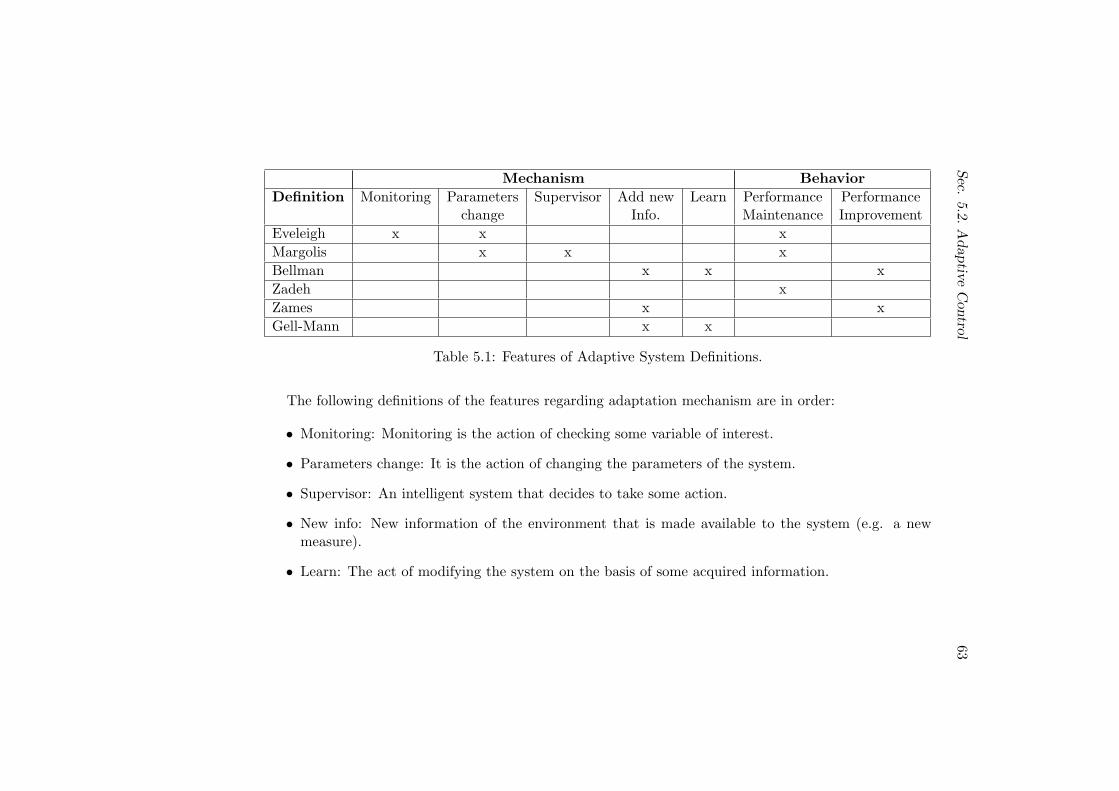
Sec.
5.2.A
dap
tive
Con
trol63
Mechanism Behavior
Definition Monitoring Parameters Supervisor Add new Learn Performance Performancechange Info. Maintenance Improvement
Eveleigh x x x
Margolis x x x
Bellman x x x
Zadeh x
Zames x x
Gell-Mann x x
Table 5.1: Features of Adaptive System Definitions.
The following definitions of the features regarding adaptation mechanism are in order:
• Monitoring: Monitoring is the action of checking some variable of interest.
• Parameters change: It is the action of changing the parameters of the system.
• Supervisor: An intelligent system that decides to take some action.
• New info: New information of the environment that is made available to the system (e.g. a newmeasure).
• Learn: The act of modifying the system on the basis of some acquired information.
64 Information Supervision of Adaptive Control Schemes
In our conceptualization of adaptive control, we focus on the fact that inorder to have an adaptive system the following actions are required:
• Acquiring information. The mechanisms related with the action of ac-quiring information comprises the Monitoring and Add new Info.
• Modifying the own system (e.g. parameters, structure, etc) on the basisof the new acquired information. This is accomplished by the mecha-nisms Parameters change and Learn.
• The system modifications allow the system to perform better than withoutmodifications. This includes both, the performance maintenance over achanging environment and the performance improvement.
At this stage it is worth to state that adaptive control does not have any todo with time varying systems or with nonlinear systems but with uncertainty.In fact the above proposed scheme is a consequence of a lack of informationas the first step of the schemes is to add new information. The lack of in-formation is not caused only by an environment information deficiency (e.g.signal spectrum has no relevant content over some frequency range) but bya system representation fault (e.g. linear model for representing a nonlinearplant). In fact a linear model can capture accurately the nonlinear behavioronly around some restricted neighborhood point. If the set point is changedthe linear model is modified.
The second point of interest of adaptive control is the information super-vision. In fact the above enumerated actions must be managed by means ofsome entity, the supervisor.
5.2.2 Supervision of Adaptive Control
The adaptive control actions mentioned above must be managed by a supervi-sor. The supervisor goal is to take the appropriate actions in order to improvesystem performance by acquiring new information by, for example, performinga new experiment. In this sense, as stated on the first section of the chapter,a supervisor is a logic that manages the control problem information flow.
The rationale behind the supervisor actions is that the acquired informa-tion helps to improve system performance. However it is not the general case
Sec. 5.2. Adaptive Control 65
that new information is useful. For example recall the concepts of Neutrality,Separability and Certainty Equivalence from stochastic control systems:
• Neutrality (Feldbaum, 1965). A stochastic control system is neutral ifthe rate of reduction of uncertainty about the states X is independentof the control u.
• Separability (Joseph and Tou, 1961). A stochastic control problem isseparable if the only information which needs to be transmitted in orderto calculate the control action is a point estimate of the current state,no information about accuracy being required.
• Certainty Equivalence (Simon, 1956). A separable problem is certainty-equivalent when the form of the control law is identical with that of thefunction specifying the optimal control law for an equivalent determin-istic problem (i.e. a problem having no uncertainties about the stateX).
The structural property of neutrality deternines that the information ofthe state is independent of the input. The main implication is that there isno reason to introduce any probing action (e.g. input experiment) in order toincrease the rate of uncertainty reduction of the system states.
The Separability property indicates that the optimal control law does notdepend on the uncertainty. Thus the parameters to be transmitted to thecontroller are just the state estimates, no its uncertainty.
The Certainty Equivalence property is a stronger property than separabil-ity. It refers to separable problems and states that the form of the optimalcontrol law equals the control law of the equivalent deterministic problem (i.e.no uncertainty of the state). It follows that the control law can be designedwithout consider stochastic effects.
Sufficient conditions on systems for being neutral, separable and certain-equivalent can be found in (Harris and Billings, 1981). Linearity is an essentialrequirement in all the above conditions. Additionally the uncertainty consid-ered is only stochastic (i.e. Gaussian noise). Notwithstanding supervisors thatmanage adaptive control schemes can indeed improve the system performanceas:
66 Information Supervision of Adaptive Control Schemes
• The problem of system identification (Ljung, 1999) is highly dependenton the experimental data used for data generation. Thus probing notonly can improve the identified model but it is a necessity (e.g. persis-tently exciting signal).
• As stated in (Harris and Billings, 1981): “It follows that adaptive control,which is an approach to non-linear problems, is concerned with problemswhich do not satisfy the known sufficient conditions for neutrality, sepa-rability or certainty equivalence and which are very unlikely to enjoy anyof the three properties.”
It then follows that the supervision of adaptive systems can indeed improvethe overall system performance. The idea is that if more information relevantfor control purposes is added, then better controllers can be designed.
5.3 Information Flow Analysis of Adaptive ControlSchemes
In this section two paradigms of adaptive control (following the adaptive con-trol definition given in the preceding section) the classical adaptive controland iterative control are studied under the information framework presentedin Chapter 4. The objective is to show the particularities of each one of theproposed schemes regarding its information flow management properties andhow the analysis permits to detect limitations and improvements of the ap-proaches.
5.3.1 Classical Adaptive Control
We refer to classical adaptive control as the adaptive control approach pre-sented in (Astrom and Wittenmark, 1989). We focus our analysis to the modelreference adaptive system (MRAS). The principal features of the scheme are:
• The performance of the system is specified by a model.
• The controller parameters are changed based on the error between theoutputs of the system and the reference model.
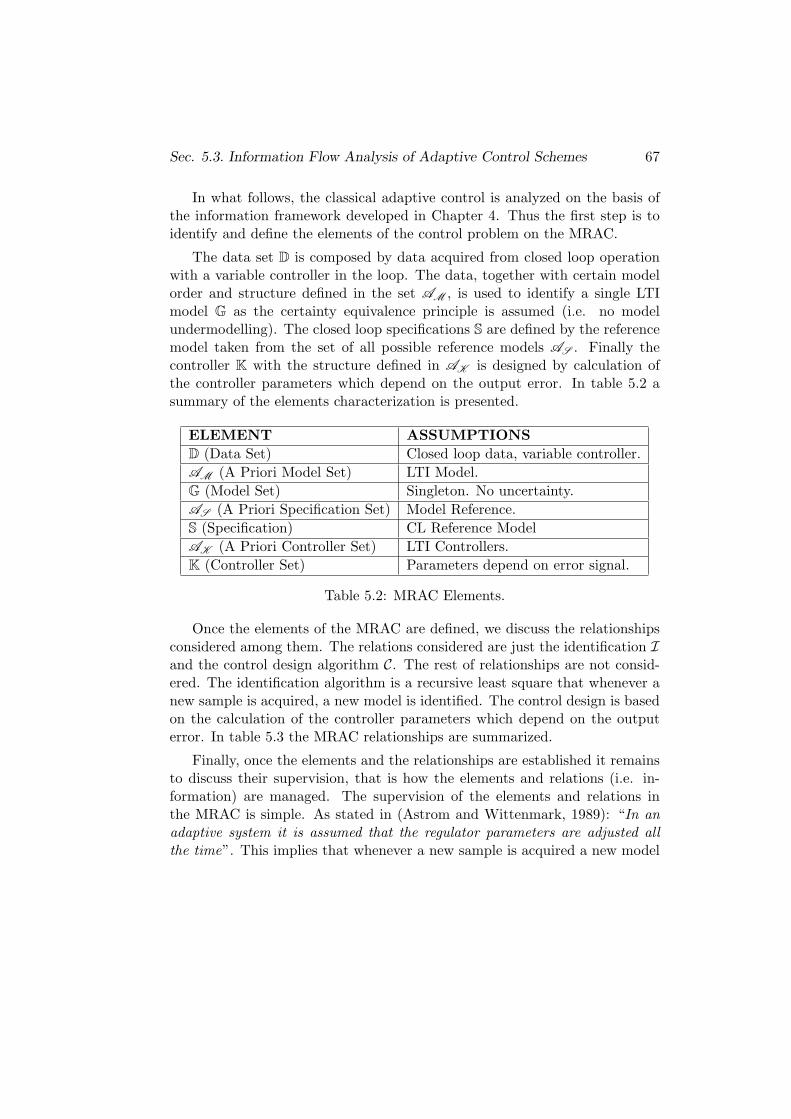
Sec. 5.3. Information Flow Analysis of Adaptive Control Schemes 67
In what follows, the classical adaptive control is analyzed on the basis ofthe information framework developed in Chapter 4. Thus the first step is toidentify and define the elements of the control problem on the MRAC.
The data set D is composed by data acquired from closed loop operationwith a variable controller in the loop. The data, together with certain modelorder and structure defined in the set AM , is used to identify a single LTImodel G as the certainty equivalence principle is assumed (i.e. no modelundermodelling). The closed loop specifications S are defined by the referencemodel taken from the set of all possible reference models AS . Finally thecontroller K with the structure defined in AK is designed by calculation ofthe controller parameters which depend on the output error. In table 5.2 asummary of the elements characterization is presented.
ELEMENT ASSUMPTIONS
D (Data Set) Closed loop data, variable controller.
AM (A Priori Model Set) LTI Model.
G (Model Set) Singleton. No uncertainty.
AS (A Priori Specification Set) Model Reference.
S (Specification) CL Reference Model
AK (A Priori Controller Set) LTI Controllers.
K (Controller Set) Parameters depend on error signal.
Table 5.2: MRAC Elements.
Once the elements of the MRAC are defined, we discuss the relationshipsconsidered among them. The relations considered are just the identification Iand the control design algorithm C. The rest of relationships are not consid-ered. The identification algorithm is a recursive least square that whenever anew sample is acquired, a new model is identified. The control design is basedon the calculation of the controller parameters which depend on the outputerror. In table 5.3 the MRAC relationships are summarized.
Finally, once the elements and the relationships are established it remainsto discuss their supervision, that is how the elements and relations (i.e. in-formation) are managed. The supervision of the elements and relations inthe MRAC is simple. As stated in (Astrom and Wittenmark, 1989): “In anadaptive system it is assumed that the regulator parameters are adjusted allthe time”. This implies that whenever a new sample is acquired a new model

68 Information Supervision of Adaptive Control Schemes
RELATIONSHIP CONSIDERED?
I (Identification) Recursive LSM
C (Controller Design) Parameters depend on error signal
O (Consistency) No
V (Model Validation) No
L (Limitations) No
M (Monitoring) No
Table 5.3: MRAC Relationships.
is identified by the recursive algorithm. Thus a new output error can be calcu-lated and the controller parameters modified accordingly. There are no otherconsiderations taken.
The way that information is managed in the MRAC adaptive control inparticular, and in the classical adaptive control in general, leads to the follow-ing problems:
• Stability Issues.
• Limited use of information sources.
• Limited management of information.
which are discussed in the next paragraphs.
Stability Issues
The stability problems of adaptive control have been recognized since thebeginning of the field. However their causes were not recognized after sometime. In (Anderson, 2005) a review on the instability causes is conducted:
• Bursting. Bursting is a phenomenon that shows transient instability. Itis caused by deficient model identification due to the lack of persistentlyexciting signals. However due to unstable behavior signals become richenough to identify a good model and the instability disappears.
Sec. 5.3. Information Flow Analysis of Adaptive Control Schemes 69
• Process interaction. On adaptive systems there are distinct processesrunning in parallel. On the one hand the controlled plant and on theother hand the identification loop. If both processes have comparabletime scales then interactions appear than can drive the system to insta-bility.
It can be concluded from the adaptive control instability problems (Anderson,2005) that the source is a misuse of information. For example a model is iden-tified with data not informative enough (i.e. bursting problem). Anotherproblem of information misuse is due to the interaction between system iden-tification and the closed loop system. In this case the information coming fromclosed loop data is affected by the controller designed on the basis of the newdata. As a result an interaction between both processes appears which canlead to instability. The framework we propose helps to tackle these questionsrelating them with information flow management.
Limited use of information sources
In adaptive schemes, the new information introduced in the controller designinformation flow is limited to new experimental data. Thus it would be benefi-cial to increase the information sources in order to achieve a more satisfactorycontroller design. For example in (Lewis et al., 1987) it is stated: “Adaptivecontrol is a promising approach to achieve performance robustness. Its presentsetting is limited: it makes use of the most structured uncertainty in which theplant model has a known form, but unknown parameters”.
This leaves room to improve the information sources on adaptive controlschemes. In (Balaguer et al., 2006b) the following improvement is proposed:“The only new information introduced in the information flow loop is throughnew experimental data. This leaves room to improve the a priori informationby checking the consistency and validating new models identified with differentmodels order and structure”.
The idea is to increase the a priori information content on the model set sothe model can be improved not only through parameters reidentification butalso by adapting the model order.
70 Information Supervision of Adaptive Control Schemes
Limited management of information
In adaptive control schemes the only relations taken into account are the modelidentification step and the controller design step. The rest of relationships arejust disregarded as can be seen from table 5.3. As a consequence the identifiedparameters are blindly replaced as soon as they are calculated. However due tothe noise effect the parameters changes can be no significant. Thus althougha new model has been identified, it could already belong to the models familyidentified in a former step, thus the following design step is meaningless as nonew information is actually present.
In (Balaguer et al., 2006b) it is proposed to identify not only a nominalmodel but also model error bounds. Thus it is possible to validate each newmodel in such a way that if the new model belongs to the already existingmodel set then no new information is present and the controller design andupdating step is not performed. In this way the controller is not modified onthe basis of non informative models.
5.3.2 Iterative Control
Iterative control is an adaptive control design scheme in the sense that i) newinformation is added to the control design procedure that ii) modifies thecontrol system (i.e. controller) in such a way that iii) better performance levelis achieved. Nonetheless the way these actions are supervised is different thanin the classical adaptive control supervision introduced above.
The iterative control procedure is as follows:
1. An experiment in closed loop (i.e. controller Ki−1 operating) is per-formed at step i and data set Di is acquired.
2. On the basis of the new data set Di a new model is identified Gi. Itis assumed that the new model Gi is more accurate, for control designpurposes, than the former model Gi−1.
3. On the basis of the new model Gi a new controller Ki is designed. Thecontroller is applied to the loop and the procedure is repeated until somestoping condition is achieved, for example certain performance level.
Iterative control is based on two main concepts:
Sec. 5.3. Information Flow Analysis of Adaptive Control Schemes 71
• If at each iteration a “better” model can be identified, a “better” con-troller can be designed (i.e. exploiting new information).
• The procedure is supervised by the control designer, with a constantcontroller in the loop, which prevents from unnoticed problems as inadaptive control (i.e. managing the information flow more safely).
Distinct iterative identification and control approaches have been pro-posed. In what follows we enumerate them and describe the identificationand control design techniques taken. The iterative control design schemesare (Bitmead, 1993):
• The Delft School (Schrama, 1992): Coprime factor identification meth-ods (Hansen et al., 1989) together with H∞ control design (Zhou, 1998)are used.
• Windsurfer approach (Albertos and Sala, 2002): Coprime factor identifi-cation methods (Hansen et al., 1989) are joined with the Internal ModelControl (IMC) design approach (Morari and Zafirou, 1990).
• Zangstuff (Zang et al., 1995): Least Square Identification (Ljung, 1999)is used with LQG control (Bitmead et al., 1990) providing a quadraticapproach.
In order to perform the analysis of the iterative control approach on thebasis of the information framework of Chapter 4 a specific scheme must bechosen, as distinct elements and relations are considered in each one of thepresented schemes. As a result we focus on the Windsurfer approach (Albertosand Sala, 2002) and its extensions (Lee et al., 1995).
Regarding the elements of the control problem, the data set D is composedby data acquired from closed loop operation with a constant controller onthe loop. The data, together with certain model order and structure definedin AM , is used to identify a single LTI model G. It is worth to mentionthat the Hansen’s identification method (Hansen et al., 1989) can lead to amodel order explosion as stated in page 154 (Albertos and Sala, 2002) thus amodel reduction step can be necessary. The key point here is that if no modelreduction is done, the model order, and thus the a priori model informationAM is defined by the algorithm and the iterations performed.

72 Information Supervision of Adaptive Control Schemes
The a priori specifications set AS is defined by the closed loop bandwidthλ. Then at each step i the specification set S is the value of the closed loopbandwidth λi.
Finally the controller K with the structure defined in AK is designed bythe Internal Model Control (IMC) approach (Morari and Zafirou, 1990). Intable 5.4 a summary of the elements characterization is presented.
ELEMENT ASSUMPTIONS
D (Data Set) Closed loop data, constant controller.
AM (A Priori Model Set) LTI Model, variable order.
G (Model Set) Singleton. No uncertainty.
AS (A Priori Specification Set) Closed loop Bandwidth.
S (Specification) λi
AK (A Priori Controller Set) LTI Controllers.
K (Controller Set) Parameters depend on model and λi.
Table 5.4: Windsurfer Iterative Control Elements.
Once the elements of the Windsurfer Iterative Control are defined, we dis-cuss the relationships among them. The relations considered are the identifica-tion I, the control design C, the model validation V, assessment of fundamentallimitations L and performance monitoring M.
The identification I is performed through a closed loop identification al-gorithm via the fractional representation (Hansen et al., 1989). The noveltyof the method is to restate the closed loop identification method as an openloop one, hence solving the well known difficulties of closed loop identifica-tion (Ljung, 1999).
The control design step C is performed by the Internal Model Control(IMC) approach (Morari and Zafirou, 1990). In this way first an H2 optimalcontroller is designed on the basis of the model at hand. Next, the optimalcontroller is extended with a low pass filter in order to account for robustnessand implementation issues. The low pass filter bandwidth is the value fixedby the specification of the closed loop bandwidth, that is λi.
Regarding the validation step V, it is performed in two distinct ways.First a classical cross-correlation validation method is applied (Soderstromand Stoica, 1989). Secondly the spectrum of the residual is compared withthe spectrum of the noise. In fact if both spectrums are similar then the

Sec. 5.3. Information Flow Analysis of Adaptive Control Schemes 73
model is validated as there is no useful information on the residual spectrum.However if the spectrum of the residual is larger than the spectrum of thenoise at some frequency band, then the model is invalidated. Moreover thisindicates that the data is rich enough in order to attempt a new identification.To sum up the validation procedure is done by joining a classical validationprocedure together with a visual comparison of the residual spectrum and thenoise spectrum.
The fundamental limitations relation L is assessed through the knowledgeof the unstable zeros of the existing model. In (Lee et al., 1995) it is seen thatit is not possible to improve the model if RHP zeroes exist. This imposes abound on the achievable closed loop bandwidth.
Finally the Monitoring action M is performed at the end of each iteration(i.e. experiment). It is the result of the monitoring action together withthe assessed fundamental limitations and control objectives what decides tostop the iterative procedure or to perform a new iteration. In table 5.5 theWindsurfer relations are summarized.
RELATIONSHIP CONSIDERED?
I (Identification) Hansen Method
C (Controller Design) IMC
O (Consistency) No
V (Model Validation) Yes
L (Limitations) Yes
M (Monitoring) Yes
Table 5.5: Windsurfer Iterative Control Relationships.
However some problems of iterative control regarding the information man-agement are:
• Necessity for Iterative Control (Boling and Makila, 1998).
• Information misuse (Balaguer and Vilanova, 2007).
Necessity for Iterative Control
In (Schrama, 1992) the iterative control is presented as a necessity for achievinghigh performance control. The technical procedure presented belongs to the
74 Information Supervision of Adaptive Control Schemes
above named “Delft School”. The claimed necessity for iterative control iscriticized in (Boling and Makila, 1998), where it is concluded the following:
“Thus this examples (it refers to (Schrama, 1992)) in the form presentedin several conferences and published in the archival literature, can neither beused as an argument for the inadequacy of open-loop identification nor for theneed of closed-loop iterations.”
To our understanding, the key point lies on the problem statement thatreads (Boling and Makila, 1998):
“It is assumed that the plant frequency response has been determined exactlyfrom experimental data at a given set of frequencies Ω.”
The assumption establishes that during the whole controller design processthe data set is both constant and noiseless. Under this assumption, and froman information point of view, the issue of open-loop vs closed-loop identifi-cation is meaningless as the data set can not be further improved. Moreoverassuming that the other information sources (e.g. the a priori model set, theidentification algorithm, etc.) are equally informative, the obtainable resultdoes not depend on iterative schemes. The fundamental issue is that if nonew information is added at each iteration then the iterative solution is justa matter of choice as the same result could be obtained by suitable one-shotprocedure.
However, without the assumption of perfect data knowledge, iterativeschemes provide information benefits:
• The frequency information content can be different at each iteration,thus at each step new data information can be acquired.
• The selection of the information elements (e.g. model order) can bebetter chosen taking into account the information amount of the problemat each step.
Thus the potential of iterative identification and control schemes lies onthe capacity of acquiring new information at each step and the feasibility ofmanaging the current information.
Information misuse
We have seen how Iterative Control (i.e. Windsurfer approach) manages theinformation of the control problem on the basis of the information theoretic
Sec. 5.3. Information Flow Analysis of Adaptive Control Schemes 75
framework. It can be seen that iterative control is much richer than adaptivecontrol regarding the elements and relationships considered. For example, thecontroller order of adaptive control is fixed meanwhile the controller order ofan iterative scheme can be variable.
Notwithstanding the more developed scheme for information managementof iterative control, it still remains to consider if the information managementis optimal in some sense. We tackle the problem by analyzing how the in-formation quantity of the elements of the control problem evolves during theiterative process.
We introduce the concept of information monotonicity on iterative iden-tification and control schemes. Roughly speaking, an iterative identificationand control scheme is monotonic if, at each iteration, the information contentof the elements is greater or, at least, equal than the information content ofthe elements at former iterations.
In order to define the concept of information monotonicity we first recallthe mathematical concept of monotonicity over sequences.
Definition 5.3.1 (Monotonic Sequence) A sequence an such that ai+1 ≥ai for every i ≥ 1, is a monotonic increasing sequence.
♦
We assume that at each time step n we have certain amount of informationof the control problem, say In. This amount of information is the informa-tion content of the elements of the control problem introduced in Chapter 4.Recalling that the information elements of the control problem are the setsA , D, G, S, K the amount of information of the control problem at step n isIn = An, Dn, Gn, Sn, Kn. The information content of the control problem ishence monotonic if at each time step i, the information content of the controlproblem at step i + 1, that is Ii+1, is equal or “greater” than the informationcontent of the control problem at time step i. It however remains to definethe order relation between information elements. It is defined as follows:
Definition 5.3.2 (Information relation) The control problem informationelement Ii+1 = Ai+1, Di+1, Gi+1, Si+1, Ki+1 is equally or more informativethan the control problem information element Ii = Ai, Di, Gi, Si, Ki, that isIi+1 Ii iff the following set inclusion follows:
76 Information Supervision of Adaptive Control Schemes
Di+1 ⊇ Di
Ai+1 ⊇ Ai
Gi+1 ⊆ Gi
Si+1 ⊆ Si
Ki+1 ⊇ Ki
♦
Remark 5.3.1 The inclusion set requirements introduced in definition 5.3.2must be accomplished for all the elements. For example if the informationelement Ii+1 increases the data set Di+1 but decrease the a priori informationset Ai+1 with respect to the information element Ii, the concept of informationincrease of the control problem is lost. However it is true that the data set hasincreased and that the a priori information set has decreased.
♦
Following the above discussion we introduce now the definition of informa-tion monotonicity of the control problem as follows:
Definition 5.3.3 (Monotonic Information) The control problem informa-tion sequence In such that Ii+1 Ii for every i ≥ 1 is a monotonic controlproblem information sequence.
♦
Remark 5.3.2 It follows from the above definitions that in order to have amonotonic increase of information of the control problem at each time step, theinformation content of all the elements of the control problem must increase orat least remain constant. In this way, classical one shot non adaptive designmethods are monotonic as, although no new information is introduced in thedesign, no already taken information is lost.
♦
As a result of definition 5.3.3, the question of information monotonicity initerative control schemes arises. In (Balaguer and Vilanova, 2007) it is shownthat, in general, iterative identification and control schemes are not informa-tion monotonic. In fact, at each new iteration step, former data, models and
Sec. 5.3. Information Flow Analysis of Adaptive Control Schemes 77
controllers are disregarded and the whole control design process starts againon the basis of the a priori information and the new experimental data set.Thus former already taken information is just disregarded so the whole processdoes not manages information in a monotonic manner.
In what follows the example taken from (Balaguer and Vilanova, 2007) ispresented. The example shows that it is possible to increase the performance(i.e. disturbance rejection) for a wider class of disturbances if former informa-tion (i.e. former model) produced by the iterative procedure is used to designthe current controller. Moreover in the example it is envisaged a methodologyto incorporate former information on the controller.
Example 5.3.1 Zang’s Example
In (Zang et al., 1995) an iterative identification and control scheme is theo-retically posed and a numerical example given. The setup of the example is asfollows: the true plant is chosen to be of the form
yt = P (z)ut + H(z)et (5.1)
with
z−1 − 1.2z−2 − 0.3z−3 (5.2)
P (z) =+0.156z−4 + 0.0845z−5
1 − 1.25z−1 + 0.4575z−2 + 0.0279z−3(5.3)
−0.0491z−4 + 0.0077z−5 (5.4)
H(z) =2
1 + 0.6121z−1(5.5)
P (z) is a fifth-order stable non-minimum phase with a single delay. et iswhite noise of unit variance. The procedure commences identifying a model ofthe plant in open loop P0. The model order to be identified is assumed to bethird order. The presented iterative control approach is then applied six timesarriving at the final model P6 used to design the definitive controller C6.
P6(z) =1.6066z−1 − 0.9120z−2 − 1.4404z−3
1 − 0.3139z−1 − 0.6349z−2 + 0.4839z−3(5.6)
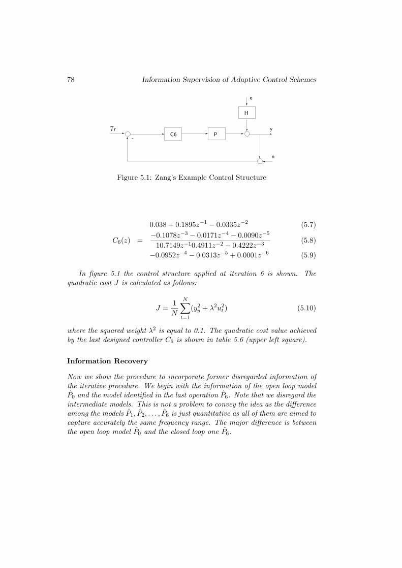
78 Information Supervision of Adaptive Control Schemes
C6 P
H
7r
e
y
n
-
Figure 5.1: Zang’s Example Control Structure
0.038 + 0.1895z−1 − 0.0335z−2 (5.7)
C6(z) =−0.1078z−3 − 0.0171z−4 − 0.0090z−5
10.7149z−10.4911z−2 − 0.4222z−3(5.8)
−0.0952z−4 − 0.0313z−5 + 0.0001z−6 (5.9)
In figure 5.1 the control structure applied at iteration 6 is shown. Thequadratic cost J is calculated as follows:
J =1
N
N∑
t=1
(y2y + λ2u2
t ) (5.10)
where the squared weight λ2 is equal to 0.1. The quadratic cost value achievedby the last designed controller C6 is shown in table 5.6 (upper left square).
Information Recovery
Now we show the procedure to incorporate former disregarded information ofthe iterative procedure. We begin with the information of the open loop modelP0 and the model identified in the last operation P6. Note that we disregard theintermediate models. This is not a problem to convey the idea as the differenceamong the models P1, P2, . . . , P6 is just quantitative as all of them are aimed tocapture accurately the same frequency range. The major difference is betweenthe open loop model P0 and the closed loop one P6.
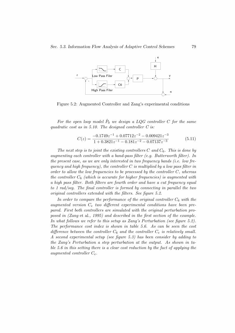
Sec. 5.3. Information Flow Analysis of Adaptive Control Schemes 79
C6
C
P
H
r
e
y
n
-
High Pass Filer
Low Pass Filer
Figure 5.2: Augmented Controller and Zang’s experimental conditions
For the open loop model P0 we design a LQG controller C for the samequadratic cost as in 5.10. The designed controller C is:
C(z) =−0.1749z−1 + 0.07712z−2 − 0.009421z−3
1 + 0.3821z−1 − 0.181z−2 − 0.07137z−3(5.11)
The next step is to joint the existing controllers C and C6. This is done byaugmenting each controller with a band-pass filter (e.g. Butterworth filter). Inthe present case, as we are only interested in two frequency bands (i.e. low fre-quency and high frequency), the controller C is multiplied by a low pass filter inorder to allow the low frequencies to be processed by the controller C, whereasthe controller C6 (which is accurate for higher frequencies) is augmented witha high pass filter. Both filters are fourth order and have a cut frequency equalto 1 rad/seg. The final controller is formed by connecting in parallel the twooriginal controllers extended with the filters. See figure 5.2.
In order to compare the performance of the original controller C6 with theaugmented version Ce two different experimental conditions have been pre-pared. First both controllers are simulated with the original perturbation pro-posed in (Zang et al., 1995) and described in the first section of the example.In what follows we refer to this setup as Zang’s Perturbation (see figure 5.2).The performance cost index is shown in table 5.6. As can be seen the costdifference between the controller C6 and the controller Ce is relatively small.A second experimental setup (see figure 5.3) has been consider by adding tothe Zang’s Perturbation a step perturbation at the output. As shown in ta-ble 5.6 in this setting there is a clear cost reduction by the fact of applying theaugmented controller Ce.
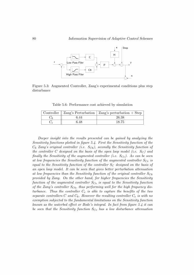
80 Information Supervision of Adaptive Control Schemes
PSfrag
C6
C
P
H
r
e Step
y
n
-
High Pass Filer
Low Pass Filer
Figure 5.3: Augmented Controller, Zang’s experimental conditions plus stepdisturbance
Table 5.6: Performance cost achieved by simulation
Controller Zang’s Perturbation Zang’s perturbation + Step
C6 6.44 26.38
Ce 6.48 18.75
Deeper insight into the results presented can be gained by analyzing theSensitivity functions plotted in figure 5.4. First the Sensitivity function of theC6 Zang’s original controller (i.e. SC6), secondly the Sensitivity function ofthe controller C designed on the basis of the open loop model (i.e. SC) andfinally the Sensitivity of the augmented controller (i.e. SCe). As can be seenat low frequencies the Sensitivity function of the augmented controller SCe isequal to the Sensitivity function of the controller SC designed on the basis ofan open loop model. It can be seen that gives better perturbation attenuationat low frequencies than the Sensitivity function of the original controller SC6
provided by Zang. On the other hand, for higher frequencies the Sensitivityfunction of the augmented controller SCe is equal to the Sensitivity functionof the Zang’s controller SC6, thus performing well for the high frequency dis-turbance. Thus the controller Ce is able to capture the benefits of the twoseparate controllers C and C6. However the resulting controller Ce is with noexemption subjected to the fundamental limitations on the Sensitivity functionknown as the waterbed effect or Bode’s integral. In fact from figure 5.4 it canbe seen that the Sensitivity function SCe has a low disturbance attenuation
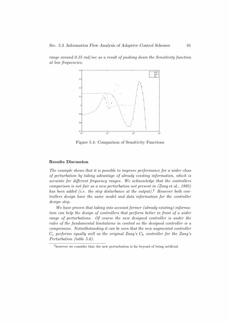
Sec. 5.3. Information Flow Analysis of Adaptive Control Schemes 81
range around 0.25 rad/sec as a result of pushing down the Sensitivity functionat low frequencies.
10−2
10−1
100
101
0.7
0.8
0.9
1
1.1
1.2
1.3
1.4SC6SCeSC
Figure 5.4: Comparison of Sensitivity Functions
Results Discussion
The example shows that it is possible to improve performance for a wider classof perturbation by taking advantage of already existing information, which isaccurate for different frequency ranges. We acknowledge that the controllerscomparison is not fair as a new perturbation not present in (Zang et al., 1995)has been added (i.e. the step disturbance at the output).2 However both con-trollers design have the same model and data information for the controllerdesign step.
We have proven that taking into account former (already existing) informa-tion can help the design of controllers that perform better in front of a widerrange of perturbations. Of course the new designed controller is under therules of the fundamental limitations in control so the designed controller is acompromise. Notwithstanding it can be seen that the new augmented controllerCe performs equally well as the original Zang’s C6 controller for the Zang’sPerturbation (table 5.6).
2however we consider that the new perturbation is far beyond of being artificial.
82 Information Supervision of Adaptive Control Schemes
5.4 Conclusions
In this chapter the concept of supervisor is presented as an entity that managesthe information flow in order to achieve certain objectives. Next the conceptof adaptive control has been reviewed and a new definition which amalgamatesformer definitions is given. Thus an adaptive system is one that performs thefollowing actions by means of a supervisor:
• “Acquiring information”. The mechanisms related with the action ofacquiring information comprises the Monitoring and Add new Info.
• “Modifying the own system (e.g. parameters, structure, etc) on thebasis of the new acquired information”. This are accomplished by themechanisms Parameters change and Learn.
• “The system modifications allow the system to perform better than with-out modifications”. This includes both, the performance maintenanceover a changing environment and the performance improvement.
Once the concept of adaptive control is generally defined and related withthe concept of information supervisor, the classical adaptive control and iter-ative control schemes are compared on the basis of the information frameworkintroduced in Chapter 4. The result on the comparison shows that:
• Both classical adaptive control and iterative control are adaptive con-trol schemes in the sense of the general definition of adaptive controlintroduced above.
• Iterative control schemes have a more developed way of supervising infor-mation than classical adaptive control. For example, the model order ofiterative schemes is not necessarily fixed as occurs on classical adaptivecontrol.
Furthermore the results of information analysis of classical adaptive controland iterative control are:
• Problems, limitations and possible improvements of classical adaptivecontrol are related with information issues as follows:
Sec. 5.4. Conclusions 83
– Stability issues of adaptive control can be explained through in-formation deficiencies. For example the bursting phenomenon ofclassical adaptive control is related to a lack of information contentif the data set (i.e. no persistently exciting signal).
– Classical adaptive control makes a limited use of the informationsources. In fact new information is added only through the data set.However the a priori information set is not modified. The controldesign process is then limited to a fixed model order and a fixedcontroller order.
– The information supervisor actions of classical adaptive control areonly the identification procedure and the control design procedure.Other actions such as model validation, assessment of fundamentallimitations, etc. are not considered. In order to improve the in-formation management of classical adaptive control it is proposedfirst to identify not only a nominal model but an error bound andsecondly to validate each new identified model against the existingmodel set. Then if the new identified model belongs to the existingmodel set no actions are necessary as no new information has beengained through the new identified model.
• The relation of iterative control with information concepts results in:
– The necessity of iterative control schemes is discussed on the basisof controversial discussion on this issue arisen in the bibliography.The rationale behind iterative control schemes in particular andadaptive control schemes in general is the capacity of adding newinformation. If a control problem is posed with all the relevant in-formation for control at hand, then adaptive control is meaningless.The power of adaptive control is to add possible useful informationfor control that was not know beforehand.
– The information management on iterative control is not monotonic.That means that although at each iteration new information is ac-quired, former information can be disregarded. In this sense it isshown by means of an example that if former information is usedfor control design, better performance levels can be achieved.

84 Information Supervision of Adaptive Control Schemes

Part II
Frequency Domain Model(In)Validation
85

Chapter 6
Frequency Domain Model(In)Validation
A new (in)validation algorithm is developed in this chapter. The (in)validationprocedure is designed to overcome the problems of classical model validationapproaches and to provide required features for information management oniterative identification and control schemes
The main idea of the algorithm is to translate the residual from the timedomain to the frequency domain and apply the frequency counterpart of thewhiteness test. The output of the algorithm results to be more informative thanthe binary answers of “Validated/Invalidated” given by classical approaches.The algorithm provides, with a probability measure, frequency ranges for whichthe model is (in)validated.
87
88 Frequency Domain Model (In)Validation
6.1 Introduction
In order to have confidence in a model, it is necessary to validate it. Dif-ferent model validation approaches exist. Their difference is based upon theassumptions on plant and models. Classical validation methods (based onclassical model identification (Ljung, 1999) (Soderstrom and Stoica, 1989))rely on statistical uncertainty assumptions due to stochastic noise only. Onthe other hand, control oriented identification methods (Chen and Gu, 2000)(i.e. H∞ identification, stochastic embedding, set membership identification,etc.) lead to validation assumptions based on bounded noise and boundedmodel undermodelling.
However in all cases above mentioned the output of the validation process isa binary result either “validated” or “invalidated”. This leads to the followingproblems (Balaguer and Vilanova, 2006b) (Balaguer and Vilanova, 2006e):
• Models are neither good nor bad. Normally models are good at cap-turing low frequency behaviour but their accuracy degrades at higherfrequencies.
• This gives no insight into why the model is not useful for the intendeduse.
• No insight on the way the model should/could be improved.
• In iterative identification and control approaches, a low order model isfitted to capture the frequency range of interest for control. Hence under-modelling is always present, which makes it difficult to apply traditionalmodel validation schemes, as stated in (Ljung, 1994).
These arguments question the suitability of classical validation approachesin general, and for Iterative Control schemes in particular. In fact the in-formation flow management of the control problem elements requires moreinformation than just a validated/invalidate test.
In order to solve the above problems, we present a new (in)validation1
1Although bibliography refers as model validation this is a misleading concept. In fact asdiscussed in (Popper, 1958) a model can not be validated but just invalidated, as future datacould invalidate it. This is a fundamental limitation of the scientific method. However inwhat follows we use the terms model validation and model invalidation indistinctly keepingin mind that a model can just be invalidated.
Sec. 6.2. Classical Model Validation 89
procedure that (in)validates the model in the frequency domain. This permitsus to ascertain at which frequency ranges the model is not invalidated. Thusthe validation answer is no longer a binary result but frequency dependent.
6.2 Classical Model Validation
The problem of assessing the validity of an identified model has been tra-ditionally linked with the problem of model order selection. The classicalmodel validation literature (Soderstrom and Stoica, 1989) (Ljung, 1994) hasapproached the problem in two ways:
• Use of plots and common sense.
• Use of statistical tests on the residuals (i.e. the difference between thereal output and the model output).
The first approach is basically based on the comparison of the data withthe model output. If both are similar then the model can be considered agood one. However there are two unavoidable reasons that prevent the modeloutput to fit data perfectly: the modelling errors and perturbations.
The second approach is to apply a hypothesis test over the residual. Ahypothesis test is a statement about a random variable. This statement isexpressed by means of two hypothesis H0 and H1. H0 is called the null hy-pothesis and H1 is the alternative hypothesis. In order to decide the validity ofeither the null hypothesis H0 or the alternative hypothesis H1, an estimationof a population parameter (e.g. mean or variance) is computed from a popu-lation sample and it is compared against the assumed population parameters.These population parameters are random variables too with certain mean andvariance. If it is likely that the computed statistic is inside the population pa-rameters distribution then H0 is accepted, otherwise H0 is rejected in favourof H1. As a result, two errors are possible: to reject H0 when it is true, thatis a false alarm (type I error or α error), or to fail to reject H0 when H0 isfalse (type II error or β error).
The null hypothesis (i.e. H0) taken on the model validation test is thehypothesis on the residual, which follows from the assumptions on the distur-bance. The more common assumptions over the residual are (Soderstrom andStoica, 1989):
90 Frequency Domain Model (In)Validation
h1 ξ(t) is a zero mean white noise.
h2 ξ(t) has a symmetric distribution.
h3 ξ(t) is independent of past inputs Eξ(t)u(τ) = 0, t > τ .
h4 ξ(t) is independent of all inputs Eξ(t)u(τ) = 0,∀t, τ .
The above assumptions lead to check two main properties, the whitenessof the residuals (i.e. h1, h2) and the cross-correlation between residuals ξ(t)and control actions u(t) (i.e. h3, h4).
Hence classical validation tests can be classified as follows
• Whiteness Test.
- Autocorrelation test. (h1)
- Testing changes of sign. (h1 and h2)
• Independence between residuals and inputs.
- Cross-correlation test of past inputs. (h3) or (h3 and h1)
- Cross-correlation test of all inputs. (h4) or (h4 and h1)
The rationale of the tests is to detect causes of variation on the residualdistinct than the ones assumed. For example if the residual is assumed tobe white noise and the test shows that the whiteness statistical hypothesis isviolated then we assume that there is a distinct cause causing the mismatch.The cause is a model error. The same example can be explained from a systemidentification perspective. On recursive least squares identification method,the residual can be interpreted as the direction through the parameters aremodified. If the residual is white then there is no clear direction to follow (i.e.erratic movement). On the other hand, if the residual is not white there is thepossibility of using the residuals to modify the parameters in a profitable way.
The result of the statistical tests above reviewed is a binary one. In factthe test either validates or invalidates the model. No further information isprovided by the test. As a result, two important drawbacks are:
• There is no information on important model aspects such as (Balaguerand Vilanova, 2006b):
Sec. 6.3. Frequency Dependent Model (In)Validation 91
– The reasons why the model is invalidate.
– How to improve the model.
– The model usefulness degree.
• In iterative identification and control schemes undermodelling is nor-mally present (Balaguer and Vilanova, 2006e). In fact as stated in (Ljung,1994): “For such a model (a model simpler that the one that minimizesthe total error) typically the bias error is the dominating contributionto the total error. Consequently, such models would normally be falsifiedduring model validation. These are then reduced complexity models”.
Thus, as a conclusion, although the theory of classical validation methodsis well developed and plenty of successful applications, it has limitations whena more informative validation procedure is required, as for example in iterativeidentification and control approaches.
6.3 Frequency Dependent Model (In)Validation
The main objective of the new proposed algorithm is to validate a model onthe frequency domain. To this end a time domain validation procedure basedon testing the residual whiteness is modified to achieve the pursued objec-tives (Balaguer and Vilanova, 2006a). The idea is as follows. It is assumedthat if the residual is white noise the model is validated because the residualcontains no further useful information that could be used to improve the modelaccuracy. Moreover it implies that there are no unmodelled dynamics as theuncertainty is due only to measurement noise. This test is usually performedin the time domain by testing the residual autocorrelation, the number of signchanges, etc. (Ljung, 1999).
The translation of the time domain whiteness test to the frequency domainis performed through two steps. Firstly we translate the time domain residualto the frequency domain by its Discrete Fourier Series. Secondly, the statis-tical properties of the spectrum of a white noise signal are calculated. Theobjective is to test if the spectrum calculated from the residual has propertiesof a white noise. As a result, one unique test in the time domain has beentranslated to N different tests in the frequency domain. We check if the kth
frequency component of the spectrum has the properties of a typical frequency
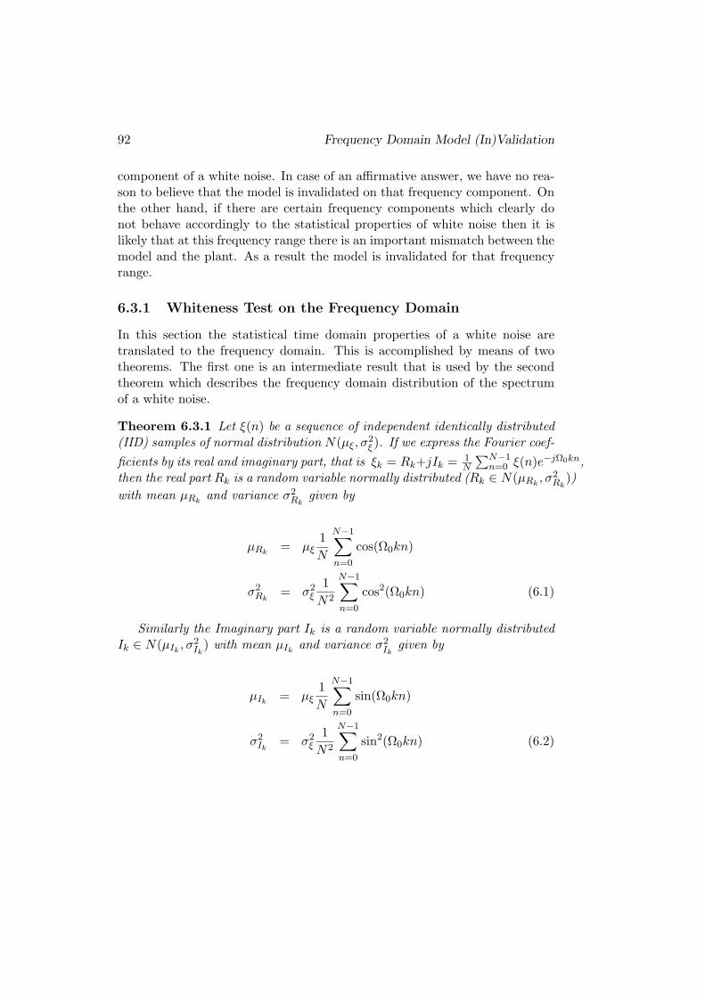
92 Frequency Domain Model (In)Validation
component of a white noise. In case of an affirmative answer, we have no rea-son to believe that the model is invalidated on that frequency component. Onthe other hand, if there are certain frequency components which clearly donot behave accordingly to the statistical properties of white noise then it islikely that at this frequency range there is an important mismatch between themodel and the plant. As a result the model is invalidated for that frequencyrange.
6.3.1 Whiteness Test on the Frequency Domain
In this section the statistical time domain properties of a white noise aretranslated to the frequency domain. This is accomplished by means of twotheorems. The first one is an intermediate result that is used by the secondtheorem which describes the frequency domain distribution of the spectrumof a white noise.
Theorem 6.3.1 Let ξ(n) be a sequence of independent identically distributed(IID) samples of normal distribution N(µξ, σ
2ξ ). If we express the Fourier coef-
ficients by its real and imaginary part, that is ξk = Rk+jIk = 1N
∑N−1n=0 ξ(n)e−jΩ0kn,
then the real part Rk is a random variable normally distributed (Rk ∈ N(µRk, σ2
Rk))
with mean µRkand variance σ2
Rkgiven by
µRk= µξ
1
N
N−1∑
n=0
cos(Ω0kn)
σ2Rk
= σ2ξ
1
N2
N−1∑
n=0
cos2(Ω0kn) (6.1)
Similarly the Imaginary part Ik is a random variable normally distributedIk ∈ N(µIk
, σ2Ik
) with mean µIkand variance σ2
Ikgiven by
µIk= µξ
1
N
N−1∑
n=0
sin(Ω0kn)
σ2Ik
= σ2ξ
1
N2
N−1∑
n=0
sin2(Ω0kn) (6.2)
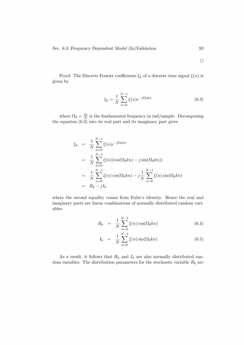
Sec. 6.3. Frequency Dependent Model (In)Validation 93
Proof: The Discrete Fourier coefficients ξk of a discrete time signal ξ(n) isgiven by
ξk =1
N
N−1∑
n=0
ξ(n)e−jΩ0kn (6.3)
where Ω0 = 2πN is the fundamental frequency in rad/sample. Decomposing
the equation (6.3) into its real part and its imaginary part gives
ξk =1
N
N−1∑
n=0
ξ(n)e−jΩ0kn
=1
N
N−1∑
n=0
ξ(n)(cos(Ω0kn) − j sin(Ω0kn))
=1
N
N−1∑
n=0
ξ(n) cos(Ω0kn) − j1
N
N−1∑
n=0
ξ(n) sin(Ω0kn)
= Rk − jIk
where the second equality comes from Euler’s identity. Hence the real andimaginary parts are linear combinations of normally distributed random vari-ables
Rk =1
N
N−1∑
n=0
ξ(n) cos(Ω0kn) (6.4)
Ik =1
N
N−1∑
n=0
ξ(n) sin(Ω0kn) (6.5)
As a result, it follows that Rk and Ik are also normally distributed ran-dom variables. The distribution parameters for the stochastic variable Rk are

94 Frequency Domain Model (In)Validation
calculated as follows (see, for example, (Box et al., 1978), page 87)
µRk= µξ
1
N
N−1∑
n=0
cos(Ω0kn)
σ2Rk
= σ2ξn
1
N2
N−1∑
n=0
cos2(Ω0kn) (6.6)
The same reasoning is applicable to the imaginary part Ik.
Remark 6.3.1 µRkis equal to zero for k ∈ 1, 2, ..., N − 1 and µR0
equalsthe mean value of the residual (i.e. µR0
= µξ). µIkis always equal to zero for
k ∈ 0, 1, 2, ..., N − 1♦
Theorem 6.3.2 The normalized squared gain M2k defined as
M2k =
(
Rk − µRk
σRk
)2
+
(
Ik − µIk
σIk
)2
(6.7)
has a χ2 distribution of 2 degrees of freedom if Rk and Ik are independent.
Proof: By definition the sum of “” independent squared random normalvariables N(0, 1) has a χ2 distribution of r degrees of freedom. Due to the
normalization of Rk and Ik, it follows thatRk−µRk
σRk
∈ N(0, 1) andIk−µIk
σIk
∈N(0, 1).
6.3.2 Procedure
The frequency domain model invalidation procedure is as follows
1. Calculate the residual as the difference of the real output and the modelestimated output (ξ(n) = y(n) − y(n)).
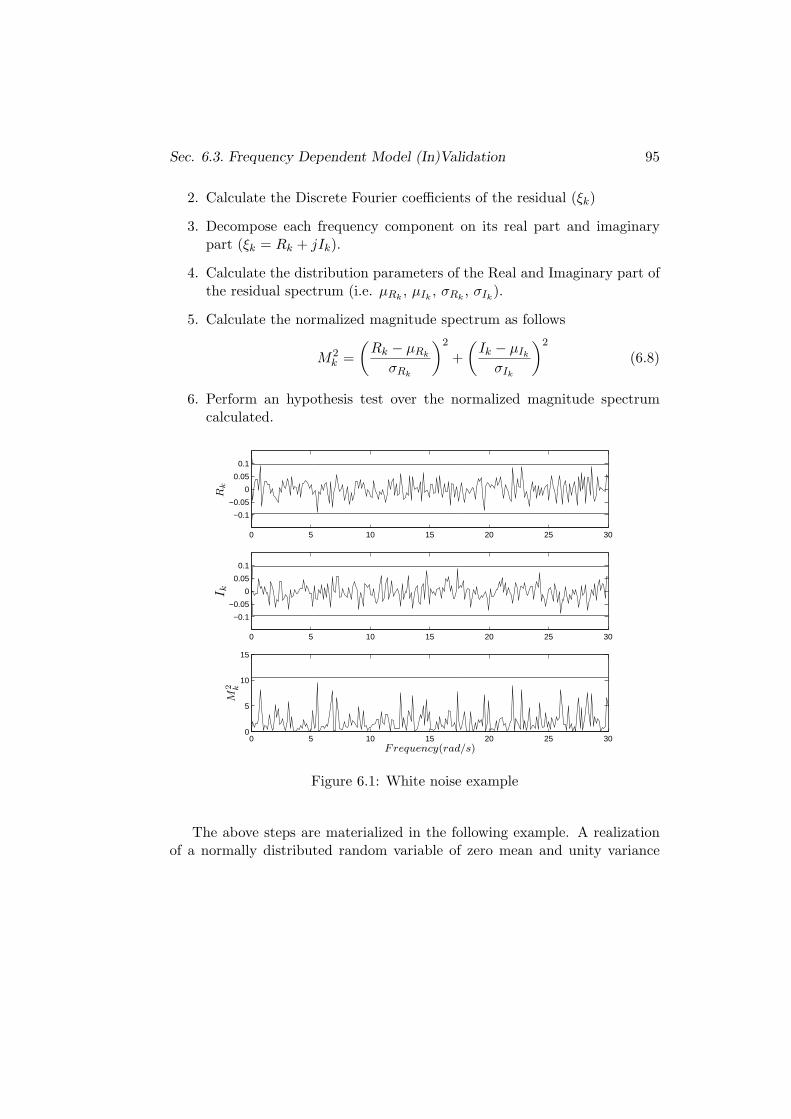
Sec. 6.3. Frequency Dependent Model (In)Validation 95
2. Calculate the Discrete Fourier coefficients of the residual (ξk)
3. Decompose each frequency component on its real part and imaginarypart (ξk = Rk + jIk).
4. Calculate the distribution parameters of the Real and Imaginary part ofthe residual spectrum (i.e. µRk
, µIk, σRk
, σIk).
5. Calculate the normalized magnitude spectrum as follows
M2k =
(
Rk − µRk
σRk
)2
+
(
Ik − µIk
σIk
)2
(6.8)
6. Perform an hypothesis test over the normalized magnitude spectrumcalculated.
0 5 10 15 20 25 30
−0.1
−0.05
0
0.05
0.1
0 5 10 15 20 25 30
−0.1
−0.05
0
0.05
0.1
0 5 10 15 20 25 300
5
10
15
Rk
I kM
2 k
Frequency(rad/s)
Figure 6.1: White noise example
The above steps are materialized in the following example. A realizationof a normally distributed random variable of zero mean and unity variance
96 Frequency Domain Model (In)Validation
is performed with 500 samples. The Discrete Fourier coefficients of the real-ization are calculated and decomposed into its real and imaginary parts (i.e.Rk, Ik). The values of Rk and Ik are shown in figure 6.1. They follow a nor-mal variable distribution with parameters given by equations (6.1)-(6.2) (i.e.Rk ∈ N(µRk
= 0, σ2Rk
= 0.001) and Ik ∈ N(µIk= 0, σ2
Ik= 0.001)). On fig-
ure 6.1 the realizations of Rk and Ik are plotted together with the 3 sigmalimits of their distribution (i.e. the 99.73% of the samples fall between theplotted limits). It can be seen that all the points fall inside this range.
Finally the normalized magnitude spectrum is calculated following equa-tion (6.8). The magnitude spectrum can be seen in figure 6.1 together with the99.5% confidence limit of the χ2
2 distribution (i.e. the 99.5% of the samples fallbetween 0 and 10.6). All the magnitude frequency components remain belowof the confidence limit so there are no reasons to invalidate the model. Thewhiteness test has passed.
Remark 6.3.2 Two important variables of the residual ξ(n) which have afundamental influence on the validation test are the sample time Ts of theresidual and the total number of samples N of the residual. The sample time Ts
imposes the maximum frequency component that can be tested by the algorithm.By the Nyquist theorem the maximum frequency is Ωmax = π
Tsrad/sec. On
the other hand the number of samples N of the residual provides the resolutionof the validation test, as the frequency range is divided in multiples of thefundamental frequency given by Ω0 = 2π
N . Thus the greater the N, the smallerthe fundamental frequency and the higher the validation test resolution.
♦
6.3.3 Hypothesis Test
The hypothesis test is the last step of the presented procedure, where thedecision of validation/invalidation of certain frequency component is taken.An hypothesis test is a statement expressed by means of two hypothesis H0
and H1. H0 is called the null hypothesis and H1 is the alternative hypothesis.The hypothesis test to be applied in our procedure is:
H0 : M2k ∈ χ2
2
H1 : M2k /∈ χ2
2 (6.9)
Sec. 6.4. Conclusions 97
The hypothesis H0 states that the normalized modulus M2k of the kth frequency
component is χ22 distributed. On the other hand the hypothesis H1 states
that the normalized modulus M2k of the kth frequency component is not χ2
2
distributed.
Remark 6.3.3 The hypothesis test stated in (6.9) is applied to each frequencycomponent, from 0 rad/sec up to the Nyquist frequency (i.e. π/Ts, where Tsis the sample time).
♦
In order to decide the validity of either the null hypothesis H0 or thealternative hypothesis H1, M2
k is computed. If it is “likely” that the value ofM2
k lies inside the χ22 distribution then H0 is accepted, otherwise H0 is rejected
in favor of H1. As a result, two errors are possible: to reject H0 when it istrue, that is a false alarm (type I error or α error), or to fail to reject H0 whenH0 is false (type II error or β error).
The term “likely” introduced above is defined by the user by choosing theconfidence limit. For example, if the confidence limit is chosen to be 10.6 thenthe 99.5% of the samples fall inside the limits. This confidence limit sets thetype I error. Following the example presented in section 6.3.2 the type I errorwas of 0.5%, that is the 0.5% of the samples of a χ2
2 should be greater than10.6 in normal conditions. The type II error is more difficult to be calculatedas it depends on the actual distribution followed by M2
k .
The hypothesis test is then simply a check that any magnitude of thenormalized spectrum is less than the test limit. If the value is greater thanthe test limit then the model results invalidate for that frequency.
6.4 Conclusions
In this chapter a new (in)validation procedure in the frequency domain hasbeen presented. The main features of the algorithm are:
• The procedure permits to validate or invalidate models over certain fre-quency ranges.
• The procedure is the translation of a time domain residual whitenesstest to a frequency dependent residual whiteness test.

98 Frequency Domain Model (In)Validation
• The validation/invalidation step is based on a hypothesis test applied toeach frequency component. This determines if certain frequency com-ponents have an unusual content that discards the model validity forthis frequency value. The acceptance/rejection decision of the frequencycomponent validity comes with a probability measure.
The new validation procedure is aimed to overcome some well known lim-itations of classical validation procedures. The advantage of the new algo-rithm hinges on its frequency dependent information in order to decide themodel validation. Thus a more informative answer is given that just a “vali-dated/invalidated” result.
Chapter 7
Control Oriented(In)Validation
Once the frequency domain model validation procedure has been presented, inthis chapter the control oriented properties of the algorithm are discussed. Inorder to obtain a meaningful model validation for control design purposes, thefrequency domain algorithm is endowed with the control oriented property bymeans of generating the residuals through a suited structure.
Once the frequency domain model validation has been provided with thecontrol oriented property the control oriented frequency dependent model val-idation (COFDMV) is analyzed regarding their properties for managing theinformation flow on iterative control schemes.
99
100 Control Oriented (In)Validation
7.1 Introduction
Model validation theory is aimed towards checking the model usefulness forsome intended use. Thus the model validation procedure should take intoaccount the model use, for example control design or prediction purposes.
In fact, it is recognized in (Skelton, 1989) that arbitrary small model errorsin open loop can lead to bad closed loop performance. On the other handlarge open loop modelling errors do not necessarily lead to bad closed loopperformance. As a result the model accuracy should be checked in such away that the intended model use is taken into account in the model validationprocedure.
An important aspect in the validation procedure to take into account theintended model use are the validation conditions. In fact validation from openloop data can provide a different result than validation with closed loop data.Furthermore it is completely different to validate an open loop model than tocompare two closed loops, the one with the model and the real one. In (Geverset al., 1999) a closed loop validation procedure is presented aimed at validatinga model for control design purposes. An open loop model is validated bycomparing two closed loops, the real one and the closed loop with the openloop model. One of the main results is that “the same model may fail tobe validated with open-loop data, while it is validated by data collected inclosed loop”. This result points out the importance of the information that isbeing validated. This is accomplished by means of setting the experimentalconditions from which data are generated.
In conclusion a model is neither good nor bad by itself but regarding itsintended use. In order to consider the model intended use in the validationprocedure the conditions for data generation must be considered. In the fol-lowing section we discuss how the new model validation procedure introducedin the preceding Chapter 6 is endowed with the control oriented property.
7.2 Control Oriented Validation
Once the fundamentals of the frequency dependent (in)validation algorithmare presented, it remains to assess the information that is being (in)validated inorder to take into account control oriented aspects as discussed in the precedingsection. In our case the model is pursued for control design purposes so the
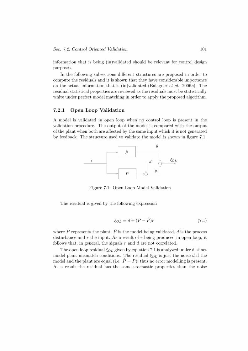
Sec. 7.2. Control Oriented Validation 101
information that is being (in)validated should be relevant for control designpurposes.
In the following subsections different structures are proposed in order tocompute the residuals and it is shown that they have considerable importanceon the actual information that is (in)validated (Balaguer et al., 2006a). Theresidual statistical properties are reviewed as the residuals must be statisticallywhite under perfect model matching in order to apply the proposed algorithm.
7.2.1 Open Loop Validation
A model is validated in open loop when no control loop is present in thevalidation procedure. The output of the model is compared with the outputof the plant when both are affected by the same input which it is not generatedby feedback. The structure used to validate the model is shown in figure 7.1.
r -
P
P
y
y
ξOLd
Figure 7.1: Open Loop Model Validation
The residual is given by the following expression
ξOL = d + (P − P )r (7.1)
where P represents the plant, P is the model being validated, d is the processdisturbance and r the input. As a result of r being produced in open loop, itfollows that, in general, the signals r and d are not correlated.
The open loop residual ξOL given by equation 7.1 is analyzed under distinctmodel plant mismatch conditions. The residual ξOL is just the noise d if themodel and the plant are equal (i.e. P = P ), thus no error modelling is present.As a result the residual has the same stochastic properties than the noise
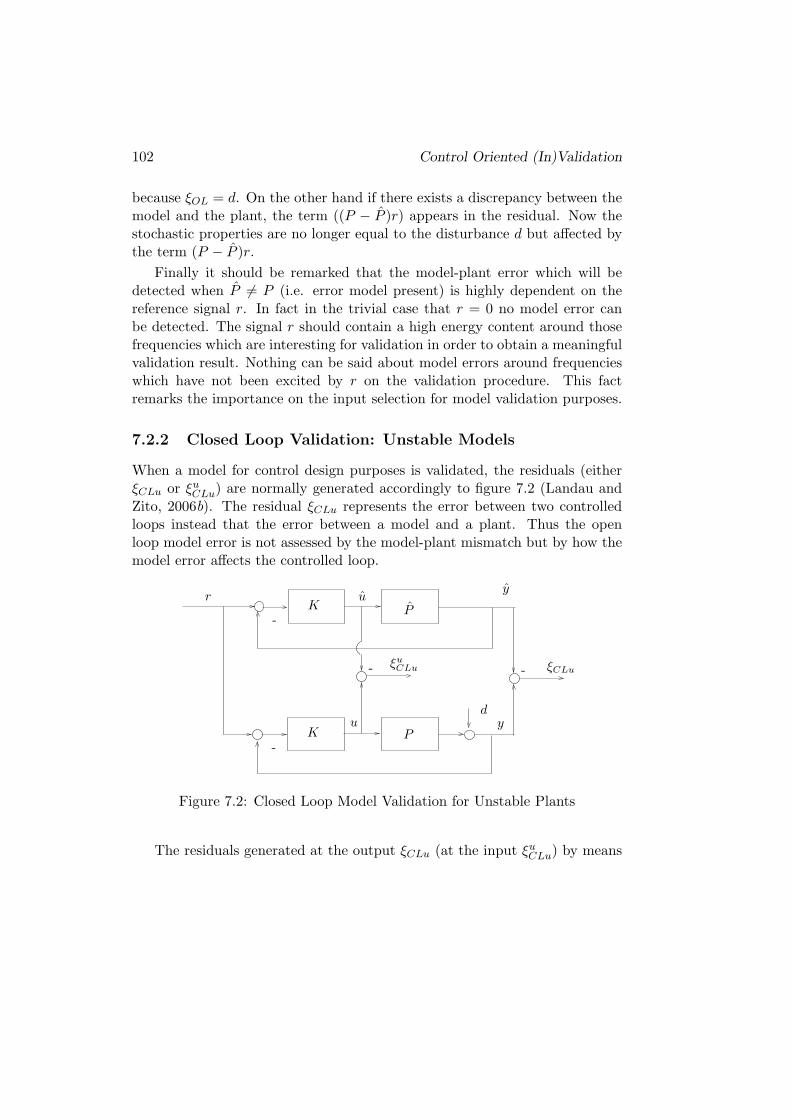
102 Control Oriented (In)Validation
because ξOL = d. On the other hand if there exists a discrepancy between themodel and the plant, the term ((P − P )r) appears in the residual. Now thestochastic properties are no longer equal to the disturbance d but affected bythe term (P − P )r.
Finally it should be remarked that the model-plant error which will bedetected when P 6= P (i.e. error model present) is highly dependent on thereference signal r. In fact in the trivial case that r = 0 no model error canbe detected. The signal r should contain a high energy content around thosefrequencies which are interesting for validation in order to obtain a meaningfulvalidation result. Nothing can be said about model errors around frequencieswhich have not been excited by r on the validation procedure. This factremarks the importance on the input selection for model validation purposes.
7.2.2 Closed Loop Validation: Unstable Models
When a model for control design purposes is validated, the residuals (eitherξCLu or ξu
CLu) are normally generated accordingly to figure 7.2 (Landau andZito, 2006b). The residual ξCLu represents the error between two controlledloops instead that the error between a model and a plant. Thus the openloop model error is not assessed by the model-plant mismatch but by how themodel error affects the controlled loop.
r
--
-
-
K
K
P
P
yu
yu
ξu
CLu ξCLu
d
Figure 7.2: Closed Loop Model Validation for Unstable Plants
The residuals generated at the output ξCLu (at the input ξuCLu) by means
Sec. 7.2. Control Oriented Validation 103
of the structure shown in figure 7.2 are:
ξCLu = Sd + KSS(P − P )r (7.2)
ξuCLu = −KSd − KKSS(P − P )r (7.3)
The residual given by equation 7.2 (7.3) in case of perfect model (i.e. P =P ) is ξCLu = Sd (ξu
CLu = −KSd). In this case the stochastic properties of theresidual ξCLu (ξu
CLu) are no longer the ones of the disturbance d. For exampleif the disturbance d is assumed white, the residual ξCLu (ξu
CLu) is alwaysautocorrelated as it is filtered by the sensitivity function S (KS) independentlyof the model-plant mismatch.
If there exists a model plant mismatch the new residual term KSS(P −P )r (KKSS(P − P )r) arises. Again, the impact of the term in the residualdepends on the reference r. However the model plant error is weighted by KSS(KKSS) thus giving more importance to the frequencies where the Sensitivityfunction has a high value, that is around the crossover frequency. Thus themodel errors are evaluated taking into account the closed loop.
The preceding discussion establishes two important facts:
• The residual generated in closed loop is suited for model validation forcontrol design purposes. Even unstable models can be validated as faras the closed loop is stable.
• The residual generated is no longer equal to the disturbance d underperfect model plant fit. This fact prevents the residual to be used in awhiteness test of any kind.
As a result, although the control oriented nature of the residuals generatedfollowing diagram 7.2 is advantageous in front of the open loop counterpart, theauto-correlation of the produced residual ξCLu (ξu
CLu) prevents from applyingany whiteness test. Accordingly the residuals thus generated are not suitedto be used by the FDMV as the validation algorithm is based on a whitenesstest in the frequency domain. In the next section a new structure is proposedin order to obtain control oriented residuals suited to be used by a whitenesstest.
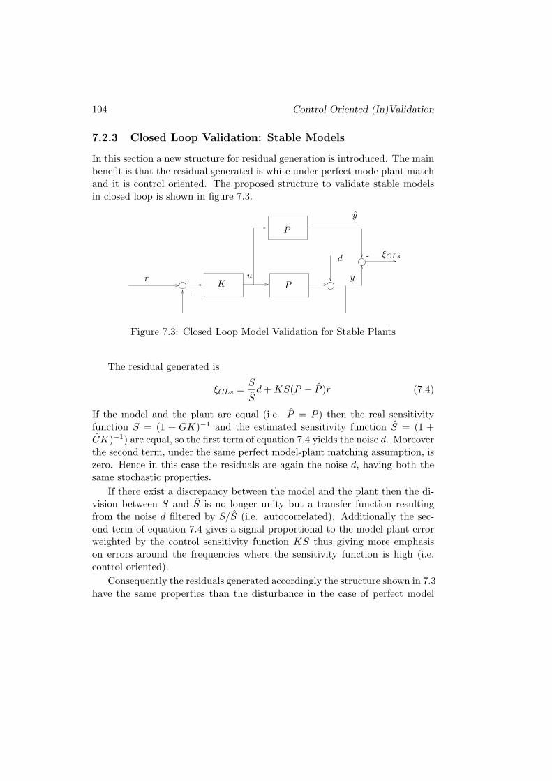
104 Control Oriented (In)Validation
7.2.3 Closed Loop Validation: Stable Models
In this section a new structure for residual generation is introduced. The mainbenefit is that the residual generated is white under perfect mode plant matchand it is control oriented. The proposed structure to validate stable modelsin closed loop is shown in figure 7.3.
r
-
-K P
P
yu
y
ξCLsd
Figure 7.3: Closed Loop Model Validation for Stable Plants
The residual generated is
ξCLs =S
Sd + KS(P − P )r (7.4)
If the model and the plant are equal (i.e. P = P ) then the real sensitivityfunction S = (1 + GK)−1 and the estimated sensitivity function S = (1 +GK)−1) are equal, so the first term of equation 7.4 yields the noise d. Moreoverthe second term, under the same perfect model-plant matching assumption, iszero. Hence in this case the residuals are again the noise d, having both thesame stochastic properties.
If there exist a discrepancy between the model and the plant then the di-vision between S and S is no longer unity but a transfer function resultingfrom the noise d filtered by S/S (i.e. autocorrelated). Additionally the sec-ond term of equation 7.4 gives a signal proportional to the model-plant errorweighted by the control sensitivity function KS thus giving more emphasison errors around the frequencies where the sensitivity function is high (i.e.control oriented).
Consequently the residuals generated accordingly the structure shown in 7.3have the same properties than the disturbance in the case of perfect model
Sec. 7.3. Model Validation on Iterative/Adaptive Schemes 105
plant matching and are control oriented. Thus if the disturbance is white itis possible to apply any whiteness test over the residuals (i.e. FDMV). Theonly drawback of the structure presented in 7.3 is that it is not feasible forunstable models, as the model P is operated in open loop.
7.3 Model Validation on Iterative/Adaptive Schemes
The objective assumed by classical model validation approaches is to ascertainthe validity of the model. Consequently if a model is validated there are noreasons to doubt of the suitability of the data set D, the a priori model infor-mation set AM and the identification algorithm I. As discussed in Chapter 2,model validation does not produce any new element of the control problem.The only relationships which transform existing elements into new ones arethe identification and the control design. The mission of the rest of the rela-tionships (e.g. model validation) are to check the validity among the elements.
Notwithstanding the model validation procedure plays a more active roleon adaptive schemes. The requirement of adding periodically new informa-tion arises new requirements on the validation procedure beyond that the“validated/invalidated” answer. The new requirements are:
• Is it possible to improve an existing model? Is the data informativeenough to attempt a new identification?
• How can the model be improved? Is the model order/structure richenough to capture the interesting features of the plant?
• How authoritative can be the controller designed on the basis of the newmodel? Which is the validity frequency range of the model?
The above requirements for iterative control can not be provided by theclassical model validation approaches above introduced because:
• No indication on the possibility to improve an existing model. Thisproblem is tackled in (Lee et al., 1995) by the use of classical validationmethods (i.e. crosscorrelation test) together with the visual comparisonof two power spectrum.
106 Control Oriented (In)Validation
• In iterative identification and control approaches a low order model isfitted to capture the frequency range of interest for control. Hence un-dermodelling is always present. This fact makes it difficult to applytraditional model validation schemes as the output of the validation pro-cedure is a binary answer (i.e. validated/no validated) (Ljung, 1994).
• No indication on how to improve the model on the next iteration (i.e.model order selection and/or input experiment design).
• No indication on the model validity range for control design (i.e. con-troller bandwidth selection).
These limitations arise the need for a more informative validation pro-cedure. In fact, the windsurfer approach to iterative control (see for exam-ple (Albertos and Sala, 2002)), is enhanced with some new features introducedin (Lee et al., 1995). Regarding model validation, two complementary vali-dation methods are applied, a time domain method and a frequency domainmethod. The time domain validation is a classical cross-correlation test be-tween the residual and the filtered input. In fact no whiteness test couldbe applied to the residual as they are generated following the structure offigure 7.2. The frequency domain method for model validation is based oncomparing two power spectrum, the noise spectrum and the residual spec-trum. When the residual spectrum is larger than the noise spectrum for somefrequency range, that means that the error cause is the undermodelling. Thusthe model is invalidated for that frequency range. Moreover the spectrumcomparison reveals frequency bands where high signal-to-noise ratio is presentand thus the data is suited to attempt a new identification procedure, at leastfor some frequency band. The frequency domain information is obtained byvisual comparison of both spectrums.
The Control Oriented Frequency Dependent Model Validation algorithm(COFDMV), that is the frequency domain validation procedure presented inthe preceding Chaptertogether with the residual generated by the structurepresented in figure 7.3, is of interest in iterative identification and controlschemes in general. The benefits of the COFDMV for the iterative identifica-tion and control schemes hinge on the frequency domain information producedby the algorithm and its control oriented nature. The COFDMV has the fol-lowing features:
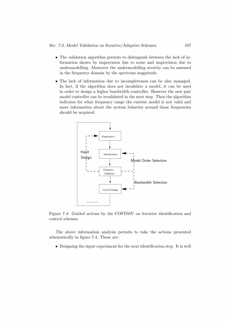
Sec. 7.3. Model Validation on Iterative/Adaptive Schemes 107
• The validation algorithm permits to distinguish between the lack of in-formation shown by imprecision due to noise and imprecision due toundermodelling. Moreover the undermodelling severity can be assessedin the frequency domain by the spectrum magnitude.
• The lack of information due to incompleteness can be also managed.In fact, if the algorithm does not invalidate a model, it can be usedin order to design a higher bandwidth controller. However the new pairmodel controller can be invalidated in the next step. Then the algorithmindicates for what frequency range the current model is not valid andmore information about the system behavior around those frequenciesshould be acquired.
Experiment i
Identification
Frequency
Validation
Control Design
i = i + 1
Input
DesignModel Order Selection
Bandwidth Selection
Figure 7.4: Guided actions by the COFDMV on iterative identification andcontrol schemes
The above information analysis permits to take the actions presentedschematically in figure 7.4. These are:
• Designing the input experiment for the next identification step. It is well
108 Control Oriented (In)Validation
known that the identified model quality is strongly dependent on theexperimental input applied to generate the data (Ljung, 1999) (Bitmeadet al., 1990). The experiment should contain high energy componentson the frequency range where the model is being invalidated if a newidentification aimed at improving the model at that frequency range ispursued. Furthermore the COFDMV indicates for what frequency bandsthe data contains meaningful information.
• Detecting model undermodelling and/or choosing model order. A higherorder model can be fitted when the current model is being invalidated.It can be done even inside the current iteration step without the need ofperforming a new experiment.
• Selecting the controller bandwidth on the controller design step. If theCOFDMV algorithm does not invalidate a model then it is feasible toincrease the model bandwidth. However the model could be invalidatedfor the new designed controller. On the other hand if a model is invali-dated at some frequency then, it is not sensible to increase the controllerbandwidth. If a higher bandwidth is desired further actions should beperformed (e.g. a new model identification).
7.4 Conclusions
In this chapter we have pointed out the importance of the final intended useof the model when a validation is performed. The frequency dependent modelvalidation algorithm proposed is control oriented because the residuals are gen-erated in a suitable way. Three distinct structures for generating the residualshave been presented. In particular the structure plot on figure 7.3 generatesresiduals which are firstly control oriented and secondly suited to be tested byany whiteness test.
Finally the control oriented frequency dependent model validation algo-rithm has been discussed on the basis of the iterative control. First the fre-quency validation proposed on the windsurfer approach has been presented.Compared with the COFDMV we can extract that the main feature of thevalidation algorithm to be useful for iterative control hinges on the frequencydomain nature of the information produced. However the main advantageof the COFDMV is that provides a qualitative assessment on the frequency

Sec. 7.4. Conclusions 109
validation/invalidation question by means of a probability measure. It fol-lows that the benefits of the COFDMV for iterative control are the bettermanagement of information flow of the control problem by:
• Designing the experimental input in order to obtain a informative dataset for some frequency band of interest (the band for what the model isnot validated).
• Increasing the model order.
• Selecting the allowable controller bandwidth with the model at hand.

110 Control Oriented (In)Validation
Chapter 8
Application Examples
The usefulness of the new frequency domain model validation approach is pre-sented by means of three examples. The first one is a classical open loopmodel validation. It shows the test when a model is invalidated. Moreover theimportance of the reference signal on model validation is stressed. Next theCOFDMV algorithm is applied to existing iterative identification and controlprocedures. Thus at each step a new model is available, it is validated regardingthe current loop controller.
111
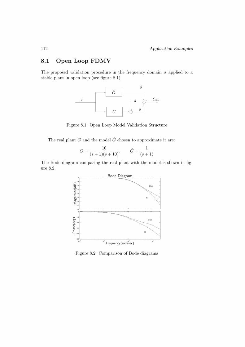
112 Application Examples
8.1 Open Loop FDMV
The proposed validation procedure in the frequency domain is applied to astable plant in open loop (see figure 8.1).
r -
G
G
y
y
ξOLd
Figure 8.1: Open Loop Model Validation Structure
The real plant G and the model G chosen to approximate it are:
G =10
(s + 1)(s + 10), G =
1
(s + 1)
The Bode diagram comparing the real plant with the model is shown in fig-ure 8.2.
−40
−35
−30
−25
−20
−15
−10
−5
0
10−2
10−1
100
101
−225
−180
−135
−90
−45
0
G
Ghat
G
Ghat
Frequency(rad/sec)
Bode Diagram
Phase
(deg
)M
agnitude(
dB)
Figure 8.2: Comparison of Bode diagrams
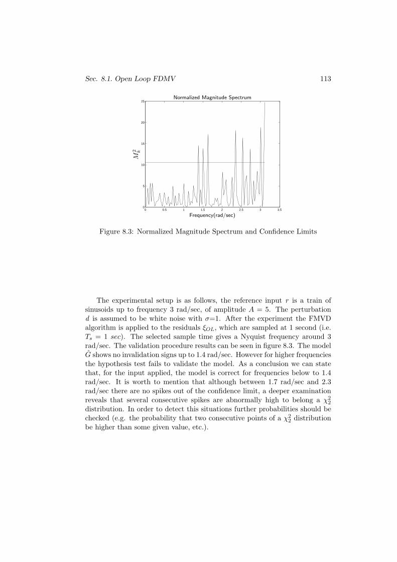
Sec. 8.1. Open Loop FDMV 113
0 0.5 1 1.5 2 2.5 3 3.50
5
10
15
20
25
Frequency(rad/sec)
M2 k
Normalized Magnitude Spectrum
Figure 8.3: Normalized Magnitude Spectrum and Confidence Limits
The experimental setup is as follows, the reference input r is a train ofsinusoids up to frequency 3 rad/sec, of amplitude A = 5. The perturbationd is assumed to be white noise with σ=1. After the experiment the FMVDalgorithm is applied to the residuals ξOL, which are sampled at 1 second (i.e.Ts = 1 sec). The selected sample time gives a Nyquist frequency around 3rad/sec. The validation procedure results can be seen in figure 8.3. The modelG shows no invalidation signs up to 1.4 rad/sec. However for higher frequenciesthe hypothesis test fails to validate the model. As a conclusion we can statethat, for the input applied, the model is correct for frequencies below to 1.4rad/sec. It is worth to mention that although between 1.7 rad/sec and 2.3rad/sec there are no spikes out of the confidence limit, a deeper examinationreveals that several consecutive spikes are abnormally high to belong a χ2
2
distribution. In order to detect this situations further probabilities should bechecked (e.g. the probability that two consecutive points of a χ2
2 distributionbe higher than some given value, etc.).
114 Application Examples
Conclusions
As a conclusion, the model G can be accepted as a good approximation ofthe plant G up to frequency 1.4 rad/sec. For higher frequencies the mismatchbetween model and plant is present up to the input bandwidth (i.e. 3 rad/sec).It should be mention that the result is input dependent. For example, fora lower amplitude of the signal r no invalidation is detected. However theresults obtained up to now can serve as a guideline to design new input signalswith suitable frequency contents for new identification steps (e.g. high energyaround the frequencies were a significant error exists, that is between 1.4rad/sec and 3 rad/sec).
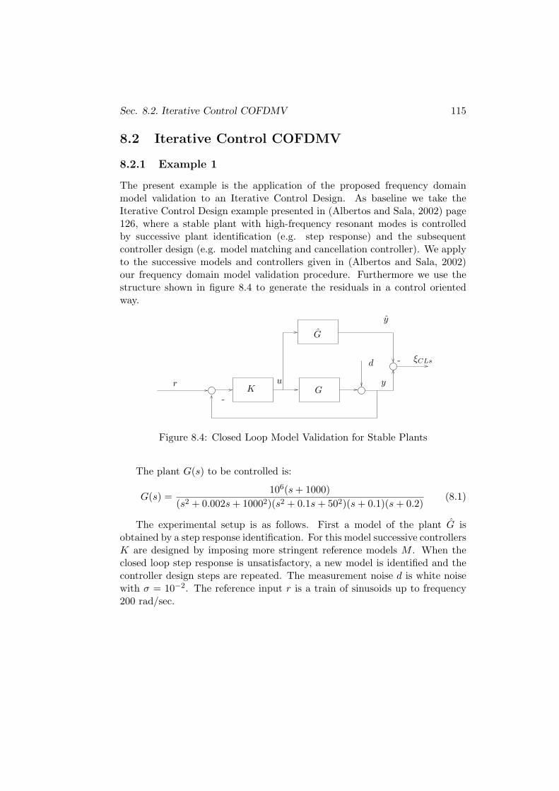
Sec. 8.2. Iterative Control COFDMV 115
8.2 Iterative Control COFDMV
8.2.1 Example 1
The present example is the application of the proposed frequency domainmodel validation to an Iterative Control Design. As baseline we take theIterative Control Design example presented in (Albertos and Sala, 2002) page126, where a stable plant with high-frequency resonant modes is controlledby successive plant identification (e.g. step response) and the subsequentcontroller design (e.g. model matching and cancellation controller). We applyto the successive models and controllers given in (Albertos and Sala, 2002)our frequency domain model validation procedure. Furthermore we use thestructure shown in figure 8.4 to generate the residuals in a control orientedway.
r
-
-K G
G
yu
y
ξCLsd
Figure 8.4: Closed Loop Model Validation for Stable Plants
The plant G(s) to be controlled is:
G(s) =106(s + 1000)
(s2 + 0.002s + 10002)(s2 + 0.1s + 502)(s + 0.1)(s + 0.2)(8.1)
The experimental setup is as follows. First a model of the plant G isobtained by a step response identification. For this model successive controllersK are designed by imposing more stringent reference models M . When theclosed loop step response is unsatisfactory, a new model is identified and thecontroller design steps are repeated. The measurement noise d is white noisewith σ = 10−2. The reference input r is a train of sinusoids up to frequency200 rad/sec.
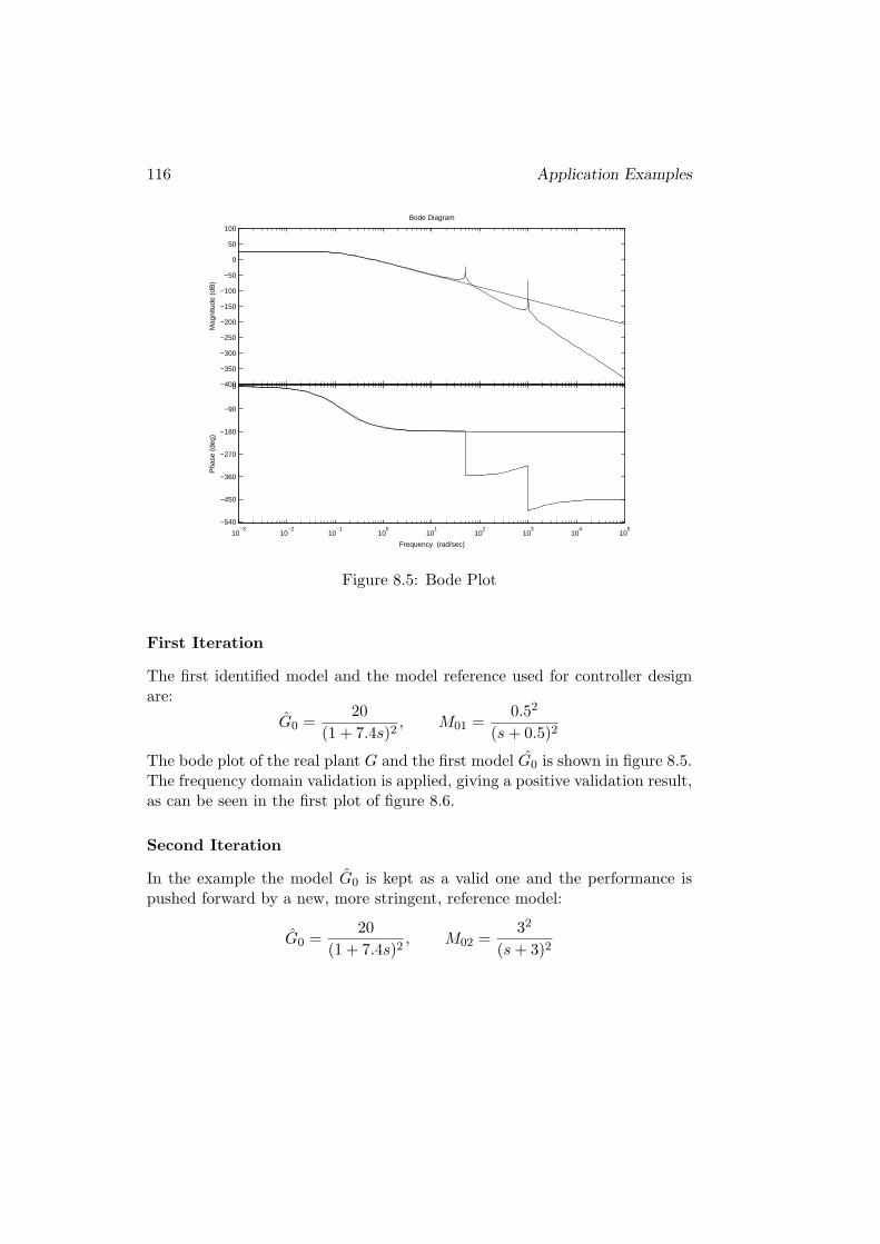
116 Application Examples
−400
−350
−300
−250
−200
−150
−100
−50
0
50
100
Mag
nitu
de (
dB)
10−3
10−2
10−1
100
101
102
103
104
105
−540
−450
−360
−270
−180
−90
0
Pha
se (
deg)
Bode Diagram
Frequency (rad/sec)
Figure 8.5: Bode Plot
First Iteration
The first identified model and the model reference used for controller designare:
G0 =20
(1 + 7.4s)2, M01 =
0.52
(s + 0.5)2
The bode plot of the real plant G and the first model G0 is shown in figure 8.5.The frequency domain validation is applied, giving a positive validation result,as can be seen in the first plot of figure 8.6.
Second Iteration
In the example the model G0 is kept as a valid one and the performance ispushed forward by a new, more stringent, reference model:
G0 =20
(1 + 7.4s)2, M02 =
32
(s + 3)2
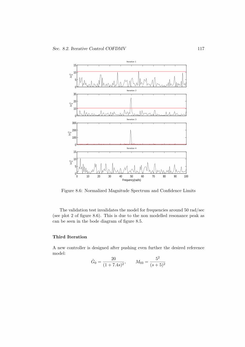
Sec. 8.2. Iterative Control COFDMV 117
0
5
10
15
0
10
20
30
0
100
200
300
0 10 20 30 40 50 60 70 80 90 1000
5
10
15
Frequency(rad/s)
M2 k
M2 k
M2 k
M2 k
Iteration 1
Iteration 2
Iteration 3
Iteration 4
Figure 8.6: Normalized Magnitude Spectrum and Confidence Limits
The validation test invalidates the model for frequencies around 50 rad/sec(see plot 2 of figure 8.6). This is due to the non modelled resonance peak ascan be seen in the bode diagram of figure 8.5.
Third Iteration
A new controller is designed after pushing even further the desired referencemodel:
G0 =20
(1 + 7.4s)2, M03 =
52
(s + 5)2
118 Application Examples
The invalidation of the model for frequencies around 50 rad/sec for this con-troller is evident (plot 3 of figure 8.6). The new controller yields an unstableclosed loop.
Fourth Iteration
In (Albertos and Sala, 2002) a new model plant is identified due to the unac-ceptable closed loop behaviour for the controller designed with the referencemodel M03. The new identified plant captures the first resonance peak of theplant.
G1 = G00.012 + 502
(s + 0.01 + 50i)(s + 0.01 − 50i),
M11 =54
(s + 5)4
The model validation result shows that now, the model is validated for all thefrequency range covered by the input (plot 4 of figure 8.6).
Conclusions
In this example the proposed COFDMV algorithm has been presented to analready developed example of iterative identification and control example. Al-though the validation algorithm has not been used to modify any of the deci-sions taken on the example, it is clear from the validation plots of figure 8.6that the algorithm detects the model frequency range that is not an accurateplant representation. At the first iteration, the pair controller-model is not in-validated. However for the second iteration it can be seen that the same modelhas problems in order to capture the plant behavior at around 50 rad/sec (i.e.the first resonant peak) due to the new more demanding controller designed.At this iteration no actions are taken although the model is clearly invalidatedfor the mentioned frequency range. On the third step the model is also in-validated around the frequency of 50 rad/sec but the normalized magnitudespectrum is one order of magnitude greater due to an even more demandingcontroller. Finally the model order is augmented with the resonant peak andthis new model together with the last designed controller is not invalidated.
Sec. 8.2. Iterative Control COFDMV 119
8.2.2 Example 2
This example deals also with the application of the COFDMV algorithm toiterative control. As a baseline we take the example of (Gunnarsson andHjalmarsson, 1994). Now it is studied the performance of the COFDMVunder distinct model order conditions. In order to accomplish the goal threeindependent iterative experiments are performed. First the whole iterativeprocedure is performed assuming a first order model of the plant. Secondlythe same iterative procedure is repeated but now considering a second ordermodel. Finally the iterative procedure is performed starting with a first ordermodel but its order is increased when necessary. In the example it is shown notonly the effect of the model undermodelling but the effect of a wrong modelidentification due to the use of feedback data (i.e. closed loop identification).
The plant to be controlled G(s) is assumed to be third order:
G(s) =2
(s + 1)
229
(s2 + 30s + 229)(8.2)
The control objective is to make the closed loop to behave as a desiredreference model, thus the controller specification is set by the model referencebandwidth wB. The controller design is performed through pole placement.
When a first order model of the plant is assumed, the reference modelselected is:
G(s) =a
(s + a)(8.3)
which imposes a bandwidth wB = a. The designed controller is discreteand designed by pole placement, thus the closed loop discrete poles are placedat z = e−Tsa. The sample time is Ts = 0.04sec.
If a second order model is assumed then the reference model is given by:
G(s) =a2
(s + a)2(8.4)
which has a bandwidth of wB = a√√
2 − 1. The rest of required poles areplaced at wB = a. As a result the discrete poles are placed at z = e−TswB .
The experimental layout is presented in figure 8.7. The reference r iswhite noise with variance σ2 = 1. The reference r is filtered through a second
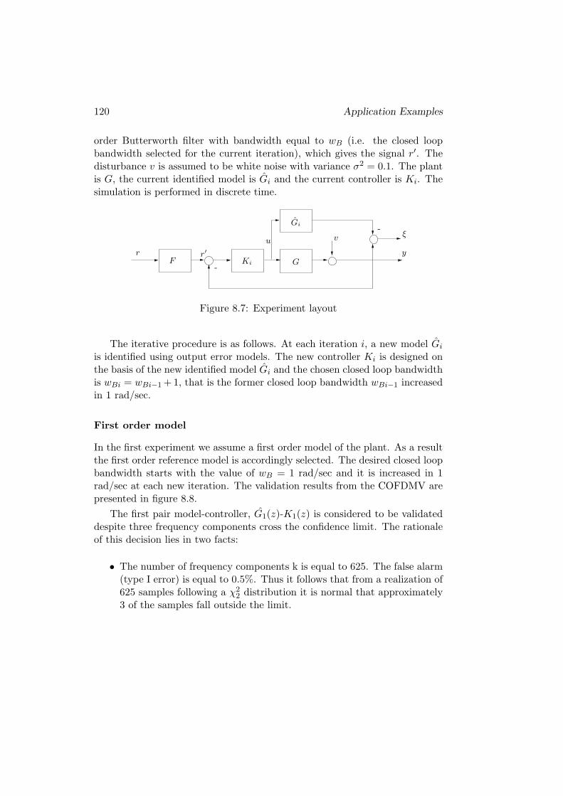
120 Application Examples
order Butterworth filter with bandwidth equal to wB (i.e. the closed loopbandwidth selected for the current iteration), which gives the signal r′. Thedisturbance v is assumed to be white noise with variance σ2 = 0.1. The plantis G, the current identified model is Gi and the current controller is Ki. Thesimulation is performed in discrete time.
r r′u v ξ
yF Ki G
Gi-
-
Figure 8.7: Experiment layout
The iterative procedure is as follows. At each iteration i, a new model Gi
is identified using output error models. The new controller Ki is designed onthe basis of the new identified model Gi and the chosen closed loop bandwidthis wBi = wBi−1 +1, that is the former closed loop bandwidth wBi−1 increasedin 1 rad/sec.
First order model
In the first experiment we assume a first order model of the plant. As a resultthe first order reference model is accordingly selected. The desired closed loopbandwidth starts with the value of wB = 1 rad/sec and it is increased in 1rad/sec at each new iteration. The validation results from the COFDMV arepresented in figure 8.8.
The first pair model-controller, G1(z)-K1(z) is considered to be validateddespite three frequency components cross the confidence limit. The rationaleof this decision lies in two facts:
• The number of frequency components k is equal to 625. The false alarm(type I error) is equal to 0.5%. Thus it follows that from a realization of625 samples following a χ2
2 distribution it is normal that approximately3 of the samples fall outside the limit.
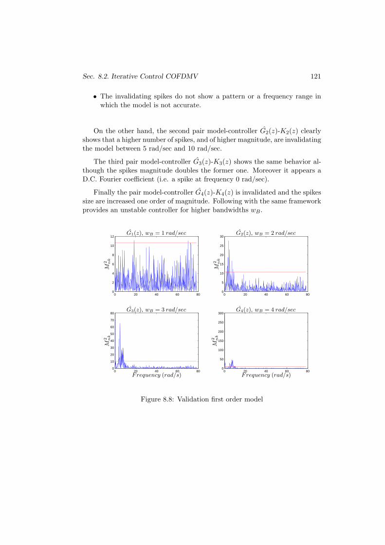
Sec. 8.2. Iterative Control COFDMV 121
• The invalidating spikes do not show a pattern or a frequency range inwhich the model is not accurate.
On the other hand, the second pair model-controller G2(z)-K2(z) clearlyshows that a higher number of spikes, and of higher magnitude, are invalidatingthe model between 5 rad/sec and 10 rad/sec.
The third pair model-controller G3(z)-K3(z) shows the same behavior al-though the spikes magnitude doubles the former one. Moreover it appears aD.C. Fourier coefficient (i.e. a spike at frequency 0 rad/sec).
Finally the pair model-controller G4(z)-K4(z) is invalidated and the spikessize are increased one order of magnitude. Following with the same frameworkprovides an unstable controller for higher bandwidths wB.
0 20 40 60 800
2
4
6
8
10
12
0 20 40 60 800
5
10
15
20
25
30
0 20 40 60 800
10
20
30
40
50
60
70
80
0 20 40 60 800
50
100
150
200
250
300
G1(z), wB = 1 rad/sec G2(z), wB = 2 rad/sec
G3(z), wB = 3 rad/sec G4(z), wB = 4 rad/sec
Frequency (rad/s)Frequency (rad/s)
M2 nk
M2 nk
M2 nk
M2 nk
Figure 8.8: Validation first order model
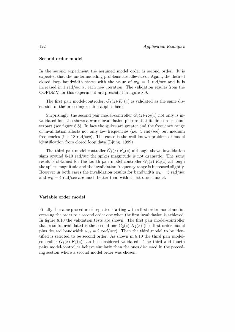
122 Application Examples
Second order model
In the second experiment the assumed model order is second order. It isexpected that the undermodelling problems are alleviated. Again, the desiredclosed loop bandwidth starts with the value of wB = 1 rad/sec and it isincreased in 1 rad/sec at each new iteration. The validation results from theCOFDMV for this experiment are presented in figure 8.9.
The first pair model-controller, G1(z)-K1(z) is validated as the same dis-cussion of the preceding section applies here.
Surprisingly, the second pair model-controller G2(z)-K2(z) not only is in-validated but also shows a worse invalidation picture that its first order coun-terpart (see figure 8.8). In fact the spikes are greater and the frequency rangeof invalidation affects not only low frequencies (i.e. 5 rad/sec) but mediumfrequencies (i.e. 18 rad/sec). The cause is the well known problem of modelidentification from closed loop data (Ljung, 1999).
The third pair model-controller G3(z)-K3(z) although shows invalidationsigns around 5-10 rad/sec the spikes magnitude is not dramatic. The sameresult is obtained for the fourth pair model-controller G4(z)-K4(z) althoughthe spikes magnitude and the invalidation frequency range is increased slightly.However in both cases the invalidation results for bandwidth wB = 3 rad/secand wB = 4 rad/sec are much better than with a first order model.
Variable order model
Finally the same procedure is repeated starting with a first order model and in-creasing the order to a second order one when the first invalidation is achieved.In figure 8.10 the validation tests are shown. The first pair model-controllerthat results invalidated is the second one G2(z)-K2(z) (i.e. first order modelplus desired bandwidth wB = 2 rad/sec). Then the third model to be iden-tified is selected to be second order. As shown in 8.10 the third pair model-controller G3(z)-K3(z) can be considered validated. The third and fourthpairs model-controller behave similarly than the ones discussed in the preced-ing section where a second model order was chosen.
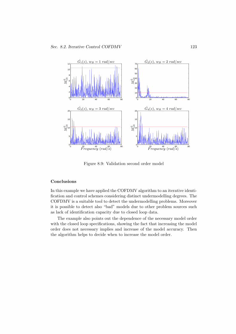
Sec. 8.2. Iterative Control COFDMV 123
0 20 40 60 800
2
4
6
8
10
12
0 20 40 60 800
10
20
30
40
50
60
70
0 20 40 60 800
5
10
15
20
0 20 40 60 800
5
10
15
20
G1(z), wB = 1 rad/sec G2(z), wB = 2 rad/sec
G3(z), wB = 3 rad/sec G4(z), wB = 4 rad/sec
Frequency (rad/s)Frequency (rad/s)
M2 nk
M2 nk
M2 nk
M2 nk
Figure 8.9: Validation second order model
Conclusions
In this example we have applied the COFDMV algorithm to an iterative identi-fication and control schemes considering distinct undermodelling degrees. TheCOFDMV is a suitable tool to detect the undermodelling problems. Moreoverit is possible to detect also “bad” models due to other problem sources suchas lack of identification capacity due to closed loop data.
The example also points out the dependence of the necessary model orderwith the closed loop specifications, showing the fact that increasing the modelorder does not necessary implies and increase of the model accuracy. Thenthe algorithm helps to decide when to increase the model order.
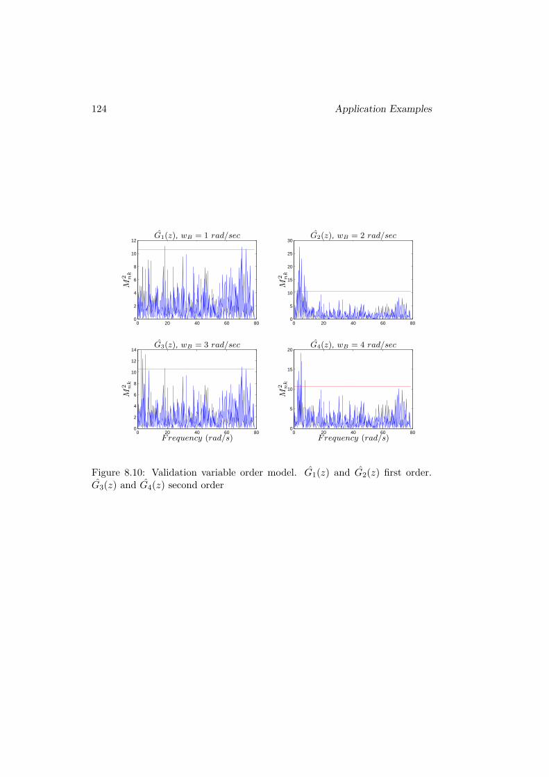
124 Application Examples
0 20 40 60 800
2
4
6
8
10
12
0 20 40 60 800
5
10
15
20
25
30
0 20 40 60 800
2
4
6
8
10
12
14
0 20 40 60 800
5
10
15
20
G1(z), wB = 1 rad/sec G2(z), wB = 2 rad/sec
G3(z), wB = 3 rad/sec G4(z), wB = 4 rad/sec
Frequency (rad/s)Frequency (rad/s)
M2 nk
M2 nk
M2 nk
M2 nk
Figure 8.10: Validation variable order model. G1(z) and G2(z) first order.G3(z) and G4(z) second order

Part III
Epilogue
125

Chapter 9
Conclusions and Perspectives
9.1 Contributions and Conclusions
The thesis presents the following contributions:
• The control problem has been formalized within the information theoreticframework. The goal has been accomplished by:
– Defining the control problem from a holistic point of view. Thatmeans that the problem has been defined taking in considerationall the possible constitutive elements and their relationships. Asa result the elements have been dissected and their relationshipsrelated with existing control theory areas.
– Reviewing the information approaches to control theory. It is con-cluded that although the information concept is a fundamental oneon control theory, it is by no means a well defined concept.
The formalization is based on very general assumptions. The advan-tage of this approach lies in the generality of the results. In fact theresults are independent of the algorithm or the mathematical charac-terization of the problem (e.g. linear vs non-linear models). In orderto derive more detailed relations, lower level mathematical assumptionsare required. The proposed framework forms the conceptual basis andprovides guidelines in which derive these schemes.
127
128 Conclusions and Perspectives
• On the basis of the information formalization of the control problem, re-lations between the information content of the elements are established.Thus theorems are proved that show necessary conditions for an informa-tion increase of certain element on the basis of the information variationof other elements. These conditions are fundamental ones affecting anyalgorithm and any mathematical formalization of the control problem.
• The concept of adaptive control is reviewed and a new definition thatamalgamates all the concepts is presented. It serves to present the basisof adaptive control which is i) acquiring information, ii) modifying thesystem on the basis of the new information iii) the modification presentsa beneficial result over the unchanged system. The definition is generaland it does not rely on any technicalities.
• Two formalizations of adaptive control, classical adaptive control anditerative control are studied under the proposed information theoreticframework. It serves to compare their similarities and differences. Thusthe information theoretic framework proposed is useful for comparingdistinct adaptive schemes as it provides a baseline for comparison. Itfollows from the results that iterative control manages the informationto be used in the control design procedure in a much richer way. Infact more questions and validation tests are performed before new in-formation is acquired and used to modify the system. On the contraryclassical adaptive control manages information in a more restricted wayas no questions about the quality or necessity of information are arisen.However it is seen that neither classical adaptive control nor iterativecontrol manage the information in a monotonic way. That means thatalthough both schemes are able to incorporate new information to theproblem, former information is discarded, so at each time step there isno guarantee that the information amount increases.
• A new model validation algorithm COFDMV is developed. The novelty ofthe algorithm is that it goes further than just a “validated/invalidated”result as the model validation is frequency dependent, thus a model isneither validated nor invalidated but the model frequency ranges validity.Moreover the algorithm helps on the management of information in thecontrol problem by i) designing the experimental energy content in orderto obtain a good model where the current one is invalidated, ii) helping
Sec. 9.2. Open Research Areas 129
in the selection of the model order, iii) deciding the expected controllerbandwidth that a model can tolerate.
The algorithm, due to its control oriented nature, results to be suitedfor iterative control schemes in which i) during the whole process severalmodels are identified and ii) the models always suffer from undermod-elling.
9.2 Open Research Areas
• The study of the control design problem by means of information con-cepts it is by no means closed. The information approach can give answerto really important questions for control theoreticians and control prac-titioners. In order to answer questions such as i) when it is necessary toperform an new identification, ii) what are the benefits expected for thenew identification, etc., it is necessary to apply the presented frameworktogether with more lower level assumptions. Thus the general abstractlypresented concepts can be posed in a more detailed way assuming moremathematical formalizations and assumptions. It is expected that posingthe presented abstract framework in a more specific basis will providemore detailed answers regarding the information flow management.
• One of the results of the thesis has been to notice the lack of informationmonotonicity of adaptive control schemes in general. It is interesting theproblem of designing an adaptive control scheme which is monotonic.The implications of monotonicity of information over the performanceof the scheme should be addressed in order to ascertain the necessity ofinformation monotonicity.
In this thesis a methodology to obtain a monotonic information itera-tive identification and control procedure has been envisaged. The ideais to form the controller joining in parallel distinct controllers whichhave been designed from models which are good for distinct frequencyranges. In order to minimize the interaction among controllers, these areaugmented with appropriate band-pass filters. The idea is that each par-ticular controller feeds back only those frequencies for which the modelthat was used for its design is good. The effect of the filters on theoverall controller is currently under investigation.
130 Conclusions and Perspectives
• The Control Oriented Frequency Dependent Control Algorithm is suitedonly for stable models due to the structure used to generate the residual.The extension of the COFDMV for unstable plant models would providea greater applicability. Currently two possible ways of accomplishing thispoint are under investigation. The first approach tries to whiten a resid-ual which has been generated by a white noise filtered by a system. Theidea is to be able to transform the residual in order to be tractable bythe current COFDMV algorithm. The second approach is more involvedand tries to developed a new frequency dependent model validation al-gorithm by translating to the frequency domain a cross-correlation timedomain model validation test. In this case the whiteness of the residualis no longer required.
9.3 Publications
The main articles on international conferences the thesis has generated are:
• P. Balaguer, R. Vilanova and R. Moreno. “The Control Problem: AFramework for Holistic Design”. 14th IEEE Mediterranean Con-ference on Control and Automation, 2006.
• P. Balaguer and R. Vilanova. “Is Iterative Control Wasting In-formation?”. 6th IEEE International Conference on Control and Au-tomation, 2007.
• P. Balaguer and R. Vilanova. “Frequency Dependent Approach toModel Validation”. 6th Asian Control Conference, 2006.
• P. Balaguer, R. Vilanova and R. Moreno. “Control Oriented Fre-quency Dependent Model Validation”. International Control Con-ference UK, 2006.
• P. Balaguer and R. Vilanova. “Quality Assessment of Models forIterative/Adaptive Control”. 45th IEEE Conference on Decisionand Control, 2006.
The thesis also has generated the following journal papers:
Sec. 9.3. Publications 131
• P. Balaguer and R. Vilanova. “Information Characterization ofthe Control Problem. Part I: The Framework”. InternationalJournal of General Systems, 2007. (submitted)
• P. Balaguer and R. Vilanova. “Information Characterization ofthe Control Problem. Part II: Analysis of Adaptive ControlSchemes”. International Journal of General Systems, 2007. (submit-ted)
• P. Balaguer and R. Vilanova. “Model Validation on Adaptive Con-trol: A Frequency Dependent Approach”. International Journalof Control, 2007. (submitted)

132 Conclusions and Perspectives
References
Albertos, P. and Sala, A., (Eds.) (2002). Iterative Identification and Control.Springer.
Anderson, Brian D.O. (2005). Failures of adaptive control theory and theirresolution. Communications in Information and Systems 5, 1–20.
Astrom, K.J. and B. Wittenmark (1989). Adaptive Control. Addison-WesleyPublishing Company.
Balaguer, P. and R. Vilanova (2006a). Frequency dependent approach to modelvalidation. In: 6th Asian Control Conference.
Balaguer, P. and R. Vilanova (2006b). Model validation on iterative iden-tification and control schemes: A frequency domain approach. In: 7thPortuguese Conference on Automatic Control.
Balaguer, P. and R. Vilanova (2006c). Monitoring plant variations with controlcharts. In: The IEEE International Conference on Methods and Modelsin Automation and Robotics.
Balaguer, P. and R. Vilanova (2006d). On-line model validation with controlcharts. In: 6th Asian Control Conference.
Balaguer, P. and R. Vilanova (2006e). Quality assessment of models for iter-ative/adaptive control. In: 45th Conference on Decision and Control.
Balaguer, P. and R. Vilanova (2007). Is iterative control wasting information?.In: 6th IEEE International Conference on Control and Automation.
Balaguer, P., R. Vilanova and R. Moreno (2006a). Control oriented frequencydependent model validation. In: International Control Conference UK.
133
134 REFERENCES
Balaguer, P., R. Vilanova and R. Moreno (2006b). The control problem: Aframework for holistic design. In: 14th Mediterranean Conference on Con-trol and Automation.
Bastin, G. and Gevers, M., (Eds.) (1997). Plenary Lectures and Mini-Courses.European Control Conference.
Bellman, R. and R. Kabala (1959). On adaptive control processes. IRE Trans-actions on Automatic Control 4, 1–9.
Bitmead, R.R. (1993). Iterative control design approaches. In: IFAC 12thTriennial World Congress.
Bitmead, R.R., M. Gevers and V. Wertz (1990). Adaptive Optimal Control.The Thinking Man’s GPC. Prentice-Hall.
Blanke, M., M. Kinnaert, J. Lunze and M. Staroswiecki (2003). Diagnosis andFault-tolerant Control. Springer.
Bode, H.W. (1945). Network Analysis and Feedback Amplifier Design. VanNostrand Co.
Boling, J.M. and P.M. Makila (1998). On control relevant criteria in Hinf
identification. IEEE Transactions on Automatic Control 43, 694–700.
Box, G.E.P., W.G Hunter and J.S. Hunter (1978). Statistics for Experimenters.An Introduction to Design, Data Analysis, and Model Building. JohnWiley & Sons.
Chaitin, G.J. (1987). Information, Randomness and Incompleteness: Paperson Algorithmic Information Theory. World Scientific, Singapore.
Chen, J. and G. Gu (2000). Control-Oriented System Identification. An H∞
Approach. John Wiley & Sons, Inc.
Devlin, K. (1991). Logic and Information. Cambridge University Press.
Doyle, J.C. and G. Stein (1981). Multivariable feedback design: Concepts fora classical/modern synthesis. IEEE Transactions on Automatic ControlAC-26, 4–16.
REFERENCES 135
Doyle, J.C., B.A. Francis and A.R. Tannenbaum (1992). Feedback ControlTheory. Macmillan Publishing Company.
Eveleigh, V.W. (1967). Adaptive control and optimization techniques. NewYork:McGraw-Hill Book Company.
Feldbaum, A.A. (1965). Optimal Control Systems. Academic Press.
Gell-Mann, M. (1995). The quark and the jaguar. W. H. Freeman.
Gevers, M. (2002). A decade of progress in iterative process control design:from theory to practice. Journal of Process Control 12, 519–531.
Gevers, M. (2006). A personal view of the development of system identifica-tion: A 30-year journey through an exciting field.. IEEE Control SystemsMagazine 26, 93–105.
Gevers, M., B. Codrons and F.D. Bruyne (1999). Model validation in closedloop. In: Proceedings of the American Control Conference.
Goodwin, G.C., D.E. Quevedo and E.I. Silva (2006). An introduction to net-worked control systems. In: The 6th Asian Control Conference.
Gunnarsson, S. and H. Hjalmarsson (1994). Some aspects of iterative iden-tification and control design schemes. Technical report. Department ofElectrical Engineering, Linkoping University, Sweden.
Hansen, F., G. Franklin and R. Kosut (1989). Closed-loop identification viathe fractional representation: Experimental design. In: American ControlConference.
Harris, C.J. and Billings, S.A., (Eds.) (1981). Self-Tunning and Adaptive Con-trol: Theory and Applications. Peter Peregrinus.
Harris, T.J., C.T. Seppala and L.D. Desborough (1999). A review of perfor-mance monitoring and assessment techniques for univariate and multi-variate control systems. Journal of Process Control 9, 1–7.
Helmicki, J., C. Jacobson and C. Nett (1991). Control oriented system identi-fication: a worst case/deterministic approach in H∞. IEEE Transactionson Automatic Control 36, 298–303.
136 REFERENCES
Hjalmarsson, H. (2005). From experiment design to closed-loop control. Auto-matica 41, 393–438.
Hjalmarsson, H., M. Gevers, S. Gunnarsson and O. Lequin (1998). Iterativefeedback tuning: Theory and applications. IEEE Control Systems Au-gust, 26–41.
Horn, J.F., D.K. Tolani, C.M. Lagoa, Q. Wang and A.Ray (2005). Probabilisticrobust control of rotorcraft. Control Engineering Practice 13, 1037–1046.
Horowitz, I.M. (1963). Synthesis of Feedback Systems. Academic Press.
Ioannou, P. and J. Sun (1996). Robust Adaptive Control. Prentice Hall.
Isermann, R. (1997). Supervision, fault-detection and fault-diagnosis methods-an introduction. Control Engineering Practice 5, 639–652.
Joseph, P.D. and J.T. Tou (1961). On linear control theory. Transactions onthe AIEE 80, 193–196.
Klir, G.J. (2006). Uncertainty and Information. Wiley-Interscience.
Klir, G.J. and M.J. Wierman (1999). Uncertainty-Base Information. Physica-Verlag.
Kolmogorov, A.N. (1965). Three approaches to the quantitative definition ofinformation. Problems of Information Transmission 1, 1–7.
Landau, I.D. (1999). From robust control to adaptive control. Control Engi-neering Practice 7, 1113–1124.
Landau, I.D. and G. Zito (2006a). Digital Control Systems. Design, Identifi-cation and Implementation.. Springer-Verlag.
Landau, I.D. and G. Zito (2006b). Digital Control Systems. Design Identifica-tion and Implementation. Springer.
Lee, W.S., B.D.O. Anderson, I.M.Y. Mareels and R.L. Kosut (1995). On somekey issues in the windsurfer approach to adaptive robust control. Auto-matica 31, 1619–1636.
REFERENCES 137
Lewis, A.H., S.I. Marcus, W.R. Perkins, P. Kokotovic, M. Athans, R.W.Brockett and A.S. Willsky (1987). Challenges to control: A collectiveview. IEEE Transactions on Automatic Control AC-32, 275–285.
Ljung, L. (1994). System identification in a MIC perspective. Modelling, Iden-tification and Control 15(3), 153–159.
Ljung, L. (1999). System Identification. Theory for the User. Prentice-Hall.
Margolis, M. and C.T. Leondes (1959). A parameter tracking servo for adap-tive control systems. IRE Transactions on Automatic Control 4, 100–111.
Morari, M. and E. Zafirou (1990). Robust Process Control. Prentice-Hall.
Newton, G., L.A. Gould and J.F. Kaiser (1957). Analytical Design of LinearFeedback Controls. Wiley.
Popper, K. (1958). The Logic of Scientific Discovery. Hutchinson & Co., Lon-don.
Qin, S. Joe (1998). Control performance monitoring- a review and assessment.Computers and Chemical Engineering 23, 173–186.
Safonov, M.G. and T.C. Tsao (1997). The unfalsified control concept andlearning. IEEE Transactions on Automatic Control 42, 843–847.
Sanchez-Pena, R.S. and M. Sznaier (1998). Robust Systems. Theory and Ap-plications. John Wikey & Sons, Inc.
Schrama, R.J.P. (1992). Accurate identification for control: The necessity ofan iterative scheme. IEEE Transactions on Automatic Control 37, 991–994.
Seron, M., J. Braslavsky and G.C. Goodwin (1997). Fundamental Limitationsin Filtering and Control. Springer.
Shannon, C.E. (1948). A mathematical theory of communciation. Bell SystemTechnical Journal 27, 623–656.
Sheridan, T.B. (1995). Reflections on information and information value. IEEETransactions on Systems, Man, and Cybernetics 25, 194–196.
138 REFERENCES
Simon, H. (1956). Dynamic programming under uncertainty with a quadraticfunction. Econometrica 24, 74–81.
Skelton, R.E. (1989). Model error concepts in control design. InternationalJournal of Control 49(5), 1725–1753.
Skogestad, S. and I. Postlethwaite (1996). Multivariable Feedback Control.Analysis and Design.. Wiley.
Soderstrom, T. and P. Stoica (1989). System Identification. Prentice Hall In-ternational Series in Systems and Control Engineering.
Stonier, T. (1990). Information and the Internal Structure of the Unvierse.Springer-Verlag.
Touchette, H. and S. Lloyd (2004). Information-theoretic approach to thestudy of control systems. Physica A 331, 140–172.
Truxal, J.G. (1963). Adaptive control. In: Proceedings of the 2nd IFAC, Basle,Switzerland.
Witsenhausen, H.S. (1971). Separation of estimation and control for discretetime systems. Proceedings of the IEEE 59, No 11, 1557–1566.
Zadeh, L.A. (1963). On the definition of adaptivity. Proceedings of the IEEE51, 569–570.
Zames, G. (1981). Feedback and optimal sensitivity: Model reference trans-formations, multiplicative seminorms, and approximate inverses. IEEETransactions on Automatic Control AC-26, 301–320.
Zames, G. (1998). Identification and adaptive control: Towards a complexity-based general theory. Systems and Control Letters 34, 141–149.
Zang, Z., R.R. Bitmead and M. Gevers (1995). Iterative weighted least-squaresidentification and weighted lqg-control. Automatica 31, 1577–1594.
Zhou, K. (1998). Essentials of Robust Control. Prentice Hall.