arX

iv:h

ep-t

h/94

0919

5v1

30

Sep

199

4

1. Classical Theory

S. W. Hawking

In these lectures Roger Penrose and I will put forward our related but rather different

viewpoints on the nature of space and time. We shall speak alternately and shall give three

lectures each, followed by a discussion on our different approaches. I should emphasize that

these will be technical lectures. We shall assume a basic knowledge of general relativity

and quantum theory.

There is a short article by Richard Feynman describing his experiences at a conference

on general relativity. I think it was the Warsaw conference in 1962. It commented very

unfavorably on the general competence of the people there and the relevance of what

they were doing. That general relativity soon acquired a much better reputation, and

more interest, is in a considerable measure because of Roger’s work. Up to then, general

relativity had been formulated as a messy set of partial differential equations in a single

coordinate system. People were so pleased when they found a solution that they didn’t

care that it probably had no physical significance. However, Roger brought in modern

concepts like spinors and global methods. He was the first to show that one could discover

general properties without solving the equations exactly. It was his first singularity theorem

that introduced me to the study of causal structure and inspired my classical work on

singularities and black holes.

I think Roger and I pretty much agree on the classical work. However, we differ in

our approach to quantum gravity and indeed to quantum theory itself. Although I’m

regarded as a dangerous radical by particle physicists for proposing that there may be loss

of quantum coherence I’m definitely a conservative compared to Roger. I take the positivist

viewpoint that a physical theory is just a mathematical model and that it is meaningless

to ask whether it corresponds to reality. All that one can ask is that its predictions should

be in agreement with observation. I think Roger is a Platonist at heart but he must answer

for himself.

Although there have been suggestions that spacetime may have a discrete structure

I see no reason to abandon the continuum theories that have been so successful. General

relativity is a beautiful theory that agrees with every observation that has been made. It

may require modifications on the Planck scale but I don’t think that will affect many of

the predictions that can be obtained from it. It may be only a low energy approximation

to some more fundemental theory, like string theory, but I think string theory has been

over sold. First of all, it is not clear that general relativity, when combined with various

other fields in a supergravity theory, can not give a sensible quantum theory. Reports of

1

the death of supergravity are exaggerations. One year everyone believed that supergravity

was finite. The next year the fashion changed and everyone said that supergravity was

bound to have divergences even though none had actually been found. My second reason

for not discussing string theory is that it has not made any testable predictions. By

contrast, the straight forward application of quantum theory to general relativity, which I

will be talking about, has already made two testable predictions. One of these predictions,

the development of small perturbations during inflation, seems to be confirmed by recent

observations of fluctuations in the microwave background. The other prediction, that

black holes should radiate thermally, is testable in principle. All we have to do is find a

primordial black hole. Unfortunately, there don’t seem many around in this neck of the

woods. If there had been we would know how to quantize gravity.

Neither of these predictions will be changed even if string theory is the ultimate

theory of nature. But string theory, at least at its current state of development, is quite

incapable of making these predictions except by appealing to general relativity as the low

energy effective theory. I suspect this may always be the case and that there may not be

any observable predictions of string theory that can not also be predicted from general

relativity or supergravity. If this is true it raises the question of whether string theory is a

genuine scientific theory. Is mathematical beauty and completeness enough in the absence

of distinctive observationally tested predictions. Not that string theory in its present form

is either beautiful or complete.

For these reasons, I shall talk about general relativity in these lectures. I shall con-

centrate on two areas where gravity seems to lead to features that are completely different

from other field theories. The first is the idea that gravity should cause spacetime to have

a begining and maybe an end. The second is the discovery that there seems to be intrinsic

gravitational entropy that is not the result of coarse graining. Some people have claimed

that these predictions are just artifacts of the semi classical approximation. They say that

string theory, the true quantum theory of gravity, will smear out the singularities and will

introduce correlations in the radiation from black holes so that it is only approximately

thermal in the coarse grained sense. It would be rather boring if this were the case. Grav-

ity would be just like any other field. But I believe it is distinctively different, because

it shapes the arena in which it acts, unlike other fields which act in a fixed spacetime

background. It is this that leads to the possibility of time having a begining. It also leads

to regions of the universe which one can’t observe, which in turn gives rise to the concept

of gravitational entropy as a measure of what we can’t know.

In this lecture I shall review the work in classical general relativity that leads to these

ideas. In the second and third lectures I shall show how they are changed and extended

2

when one goes to quantum theory. Lecture two will be about black holes and lecture three

will be on quantum cosmology.

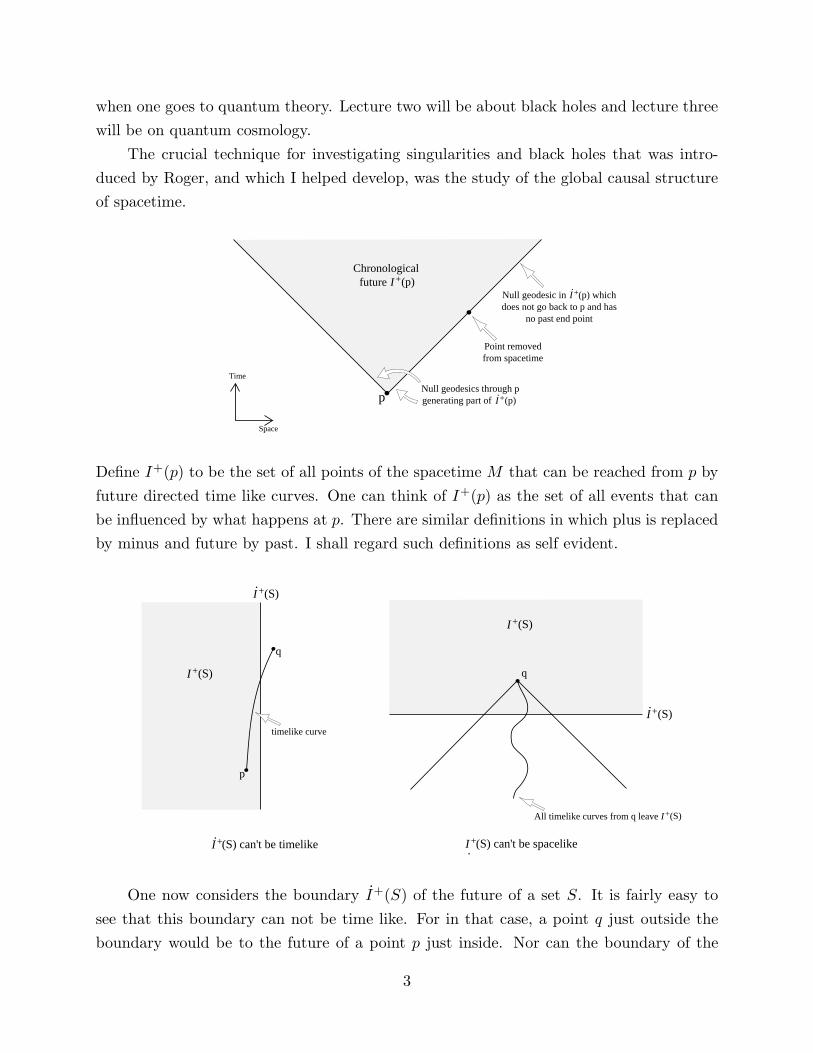
The crucial technique for investigating singularities and black holes that was intro-

duced by Roger, and which I helped develop, was the study of the global causal structure

of spacetime.

Time

Space

Null geodesics through pgenerating part of

Null geodesic in (p) whichdoes not go back to p and has

no past end point

Point removedfrom spacetime

Chronologicalfuture

p +.I (p)

+I (p)+

.I

Define I+(p) to be the set of all points of the spacetime M that can be reached from p by

future directed time like curves. One can think of I+(p) as the set of all events that can

be influenced by what happens at p. There are similar definitions in which plus is replaced

by minus and future by past. I shall regard such definitions as self evident.

q

p

+.I (S)

.

timelike curve

+I (S)

+I (S) can't be timelike

q

+.I (S)

.

+I (S)

+I (S) can't be spacelike

All timelike curves from q leave+I (S)

One now considers the boundary I+(S) of the future of a set S. It is fairly easy to

see that this boundary can not be time like. For in that case, a point q just outside the

boundary would be to the future of a point p just inside. Nor can the boundary of the

3

future be space like, except at the set S itself. For in that case every past directed curve

from a point q, just to the future of the boundary, would cross the boundary and leave the

future of S. That would be a contradiction with the fact that q is in the future of S.

q

+.I (S)null geodesic segment in

+I (S)

q

+I (S)

+.I (S)null geodesic segment in

+.I (S)future end point of generators of

One therefore concludes that the boundary of the future is null apart from at S itself.

More precisely, if q is in the boundary of the future but is not in the closure of S there

is a past directed null geodesic segment through q lying in the boundary. There may be

more than one null geodesic segment through q lying in the boundary, but in that case q

will be a future end point of the segments. In other words, the boundary of the future of

S is generated by null geodesics that have a future end point in the boundary and pass

into the interior of the future if they intersect another generator. On the other hand, the

null geodesic generators can have past end points only on S. It is possible, however, to

have spacetimes in which there are generators of the boundary of the future of a set S that

never intersect S. Such generators can have no past end point.

A simple example of this is Minkowski space with a horizontal line segment removed.

If the set S lies to the past of the horizontal line, the line will cast a shadow and there

will be points just to the future of the line that are not in the future of S. There will be

a generator of the boundary of the future of S that goes back to the end of the horizontal

4

+.I

+I (S)

S

line removed fromMinkowski space

generator of (S)with no end point on S

+.Igenerators of (S)

with past end point on S

line. However, as the end point of the horizontal line has been removed from spacetime,

this generator of the boundary will have no past end point. This spacetime is incomplete,

but one can cure this by multiplying the metric by a suitable conformal factor near the

end of the horizontal line. Although spaces like this are very artificial they are important

in showing how careful you have to be in the study of causal structure. In fact Roger

Penrose, who was one of my PhD examiners, pointed out that a space like that I have just

described was a counter example to some of the claims I made in my thesis.

To show that each generator of the boundary of the future has a past end point on

the set one has to impose some global condition on the causal structure. The strongest

and physically most important condition is that of global hyperbolicity.

q

p

∩+I (p)_

I (q)

An open set U is said to be globally hyperbolic if:

1) for every pair of points p and q in U the intersection of the future of p and the past

of q has compact closure. In other words, it is a bounded diamond shaped region.

2) strong causality holds on U . That is there are no closed or almost closed time like

curves contained in U .

5

p

every timelike curveintersects (t)

(t)

Σ

Σ

The physical significance of global hyperbolicity comes from the fact that it implies

that there is a family of Cauchy surfaces Σ(t) for U . A Cauchy surface for U is a space

like or null surface that intersects every time like curve in U once and once only. One can

predict what will happen in U from data on the Cauchy surface, and one can formulate a

well behaved quantum field theory on a globally hyperbolic background. Whether one can

formulate a sensible quantum field theory on a non globally hyperbolic background is less

clear. So global hyperbolicity may be a physical necessity. But my view point is that one

shouldn’t assume it because that may be ruling out something that gravity is trying to

tell us. Rather one should deduce that certain regions of spacetime are globally hyperbolic

from other physically reasonable assumptions.

The significance of global hyperbolicity for singularity theorems stems from the fol-

lowing.

q

pgeodesic of

maximum length

6

Let U be globally hyperbolic and let p and q be points of U that can be joined by a

time like or null curve. Then there is a time like or null geodesic between p and q which

maximizes the length of time like or null curves from p to q. The method of proof is to

show the space of all time like or null curves from p to q is compact in a certain topology.

One then shows that the length of the curve is an upper semi continuous function on this

space. It must therefore attain its maximum and the curve of maximum length will be a

geodesic because otherwise a small variation will give a longer curve.

q

r

p

geodesic

point conjugateto p along

neighbouringgeodesic

γ

γ

p

q

r

non-minimalgeodesic

minimal geodesicwithout conjugate points

point conjugate to p

One can now consider the second variation of the length of a geodesic γ. One can show

that γ can be varied to a longer curve if there is an infinitesimally neighbouring geodesic

from p which intersects γ again at a point r between p and q. The point r is said to be

conjugate to p. One can illustrate this by considering two points p and q on the surface of

the Earth. Without loss of generality one can take p to be at the north pole. Because the

Earth has a positive definite metric rather than a Lorentzian one, there is a geodesic of

minimal length, rather than a geodesic of maximum length. This minimal geodesic will be

a line of longtitude running from the north pole to the point q. But there will be another

geodesic from p to q which runs down the back from the north pole to the south pole and

then up to q. This geodesic contains a point conjugate to p at the south pole where all the

geodesics from p intersect. Both geodesics from p to q are stationary points of the length

under a small variation. But now in a positive definite metric the second variation of a

geodesic containing a conjugate point can give a shorter curve from p to q. Thus, in the

example of the Earth, we can deduce that the geodesic that goes down to the south pole

and then comes up is not the shortest curve from p to q. This example is very obvious.

However, in the case of spacetime one can show that under certain assumptions there

7

ought to be a globally hyperbolic region in which there ought to be conjugate points on

every geodesic between two points. This establishes a contradiction which shows that the

assumption of geodesic completeness, which can be taken as a definition of a non singular

spacetime, is false.

The reason one gets conjugate points in spacetime is that gravity is an attractive force.

It therefore curves spacetime in such a way that neighbouring geodesics are bent towards

each other rather than away. One can see this from the Raychaudhuri or Newman-Penrose

equation, which I will write in a unified form.

Raychaudhuri - Newman - Penrose equation

dρ

dv= ρ2 + σijσij +

1

nRabl

alb

where n = 2 for null geodesics

n = 3 for timelike geodesics

Here v is an affine parameter along a congruence of geodesics, with tangent vector la

which are hypersurface orthogonal. The quantity ρ is the average rate of convergence of

the geodesics, while σ measures the shear. The term Rablalb gives the direct gravitational

effect of the matter on the convergence of the geodesics.

Einstein equation

Rab −1

2gabR = 8πTab

Weak Energy Condition

Tabvavb ≥ 0

for any timelike vector va.

By the Einstein equations, it will be non negative for any null vector la if the matter obeys

the so called weak energy condition. This says that the energy density T00 is non negative

in any frame. The weak energy condition is obeyed by the classical energy momentum

tensor of any reasonable matter, such as a scalar or electro magnetic field or a fluid with

8

a reasonable equation of state. It may not however be satisfied locally by the quantum

mechanical expectation value of the energy momentum tensor. This will be relevant in my

second and third lectures.

Suppose the weak energy condition holds, and that the null geodesics from a point p

begin to converge again and that ρ has the positive value ρ0. Then the Newman Penrose

equation would imply that the convergence ρ would become infinite at a point q within an

affine parameter distance 1ρ0

if the null geodesic can be extended that far.

If ρ = ρ0 at v = v0 then ρ ≥ 1ρ−1+v0−v

. Thus there is a conjugate point

before v = v0 + ρ−1.

q

pneighbouring geodesics

meeting at q

future end pointof in (p)

crossing regionof light cone

inside (p)

+Iγ

γ +I

Infinitesimally neighbouring null geodesics from p will intersect at q. This means the point

q will be conjugate to p along the null geodesic γ joining them. For points on γ beyond

the conjugate point q there will be a variation of γ that gives a time like curve from p.

Thus γ can not lie in the boundary of the future of p beyond the conjugate point q. So γ

will have a future end point as a generator of the boundary of the future of p.

The situation with time like geodesics is similar, except that the strong energy con-

dition that is required to make Rablalb non negative for every time like vector la is, as

its name suggests, rather stronger. It is still however physically reasonable, at least in an

averaged sense, in classical theory. If the strong energy condition holds, and the time like

geodesics from p begin converging again, then there will be a point q conjugate to p.

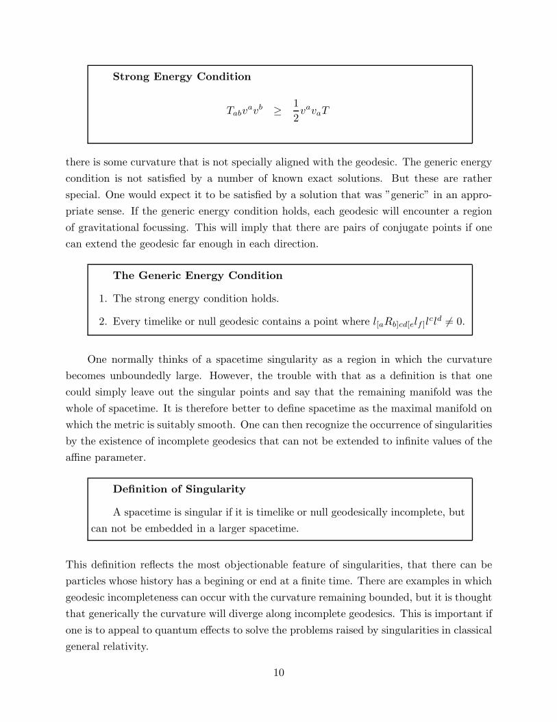
Finally there is the generic energy condition. This says that first the strong energy

condition holds. Second, every time like or null geodesic encounters some point where

9

Strong Energy Condition

Tabvavb ≥

1

2vavaT

there is some curvature that is not specially aligned with the geodesic. The generic energy

condition is not satisfied by a number of known exact solutions. But these are rather

special. One would expect it to be satisfied by a solution that was ”generic” in an appro-

priate sense. If the generic energy condition holds, each geodesic will encounter a region

of gravitational focussing. This will imply that there are pairs of conjugate points if one

can extend the geodesic far enough in each direction.

The Generic Energy Condition

1. The strong energy condition holds.

2. Every timelike or null geodesic contains a point where l[aRb]cd[elf ]lcld 6= 0.

One normally thinks of a spacetime singularity as a region in which the curvature

becomes unboundedly large. However, the trouble with that as a definition is that one

could simply leave out the singular points and say that the remaining manifold was the

whole of spacetime. It is therefore better to define spacetime as the maximal manifold on

which the metric is suitably smooth. One can then recognize the occurrence of singularities

by the existence of incomplete geodesics that can not be extended to infinite values of the

affine parameter.

Definition of Singularity

A spacetime is singular if it is timelike or null geodesically incomplete, but

can not be embedded in a larger spacetime.

This definition reflects the most objectionable feature of singularities, that there can be

particles whose history has a begining or end at a finite time. There are examples in which

geodesic incompleteness can occur with the curvature remaining bounded, but it is thought

that generically the curvature will diverge along incomplete geodesics. This is important if

one is to appeal to quantum effects to solve the problems raised by singularities in classical

general relativity.

10

Between 1965 and 1970 Penrose and I used the techniques I have described to prove

a number of singularity theorems. These theorems had three kinds of conditions. First

there was an energy condition such as the weak, strong or generic energy conditions. Then

there was some global condition on the causal structure such as that there shouldn’t be

any closed time like curves. And finally, there was some condition that gravity was so

strong in some region that nothing could escape.

Singularity Theorems

1. Energy condition.

2. Condition on global structure.

3. Gravity strong enough to trap a region.

This third condition could be expressed in various ways.

outgoing raysdiverging

outgoing raysdiverging

ingoing raysconverging

ingoing and outgoingrays converging

Normal closed 2 surface

Closed trapped surface

One way would be that the spatial cross section of the universe was closed, for then there

was no outside region to escape to. Another was that there was what was called a closed

trapped surface. This is a closed two surface such that both the ingoing and out going null

geodesics orthogonal to it were converging. Normally if you have a spherical two surface

11

in Minkowski space the ingoing null geodesics are converging but the outgoing ones are

diverging. But in the collapse of a star the gravitational field can be so strong that the

light cones are tipped inwards. This means that even the out going null geodesics are

converging.

The various singularity theorems show that spacetime must be time like or null

geodesically incomplete if different combinations of the three kinds of conditions hold.

One can weaken one condition if one assumes stronger versions of the other two. I shall

illustrate this by describing the Hawking-Penrose theorem. This has the generic energy

condition, the strongest of the three energy conditions. The global condition is fairly weak,

that there should be no closed time like curves. And the no escape condition is the most

general, that there should be either a trapped surface or a closed space like three surface.

qevery past directedtimelike curve from q

intersects S

H (S)

D (S)

S

+

+

For simplicity, I shall just sketch the proof for the case of a closed space like three

surface S. One can define the future Cauchy development D+(S) to be the region of points

q from which every past directed time like curve intersects S. The Cauchy development

is the region of spacetime that can be predicted from data on S. Now suppose that the

future Cauchy development was compact. This would imply that the Cauchy development

would have a future boundary called the Cauchy horizon, H+(S). By an argument similar

to that for the boundary of the future of a point the Cauchy horizon will be generated by

null geodesic segments without past end points.

However, since the Cauchy development is assumed to be compact, the Cauchy horizon

will also be compact. This means that the null geodesic generators will wind round and

12

H (S)+

limit null geodesicλ

round inside a compact set. They will approach a limit null geodesic λ that will have

no past or future end points in the Cauchy horizon. But if λ were geodesically complete

the generic energy condition would imply that it would contain conjugate points p and

q. Points on λ beyond p and q could be joined by a time like curve. But this would be

a contradiction because no two points of the Cauchy horizon can be time like separated.

Therefore either λ is not geodesically complete and the theorem is proved or the future

Cauchy development of S is not compact.

In the latter case one can show there is a future directed time like curve, γ from S that

never leaves the future Cauchy development of S. A rather similar argument shows that

γ can be extended to the past to a curve that never leaves the past Cauchy development

D−(S).

Now consider a sequence of point xn on γ tending to the past and a similar sequence yn

tending to the future. For each value of n the points xn and yn are time like separated and

are in the globally hyperbolic Cauchy development of S. Thus there is a time like geodesic

of maximum length λn from xn to yn. All the λn will cross the compact space like surface

S. This means that there will be a time like geodesic λ in the Cauchy development which is

a limit of the time like geodesics λn. Either λ will be incomplete, in which case the theorem

is proved. Or it will contain conjugate poin because of the generic energy condition. But

in that case λn would contain conjugate points for n sufficiently large. This would be

a contradiction because the λn are supposed to be curves of maximum length. One can

therefore conclude that the spacetime is time like or null geodesically incomplete. In other

words there is a singularity.

The theorems predict singularities in two situations. One is in the future in the

13

point at infinity

point at infinity

S

timelike curve

H (S)+

H (S)_

D (S)_

D (S)+

γ

λlimit geodesic

y

n

n

x

gravitational collapse of stars and other massive bodies. Such singularities would be an

14

end of time, at least for particles moving on the incomplete geodesics. The other situation

in which singularities are predicted is in the past at the begining of the present expansion of

the universe. This led to the abandonment of attempts (mainly by the Russians) to argue

that there was a previous contracting phase and a non singular bounce into expansion.

Instead almost everyone now believes that the universe, and time itself, had a begining at

the Big Bang. This is a discovery far more important than a few miscellaneous unstable

particles but not one that has been so well recognized by Nobel prizes.

The prediction of singularities means that classical general relativity is not a complete

theory. Because the singular points have to be cut out of the spacetime manifold one can

not define the field equations there and can not predict what will come out of a singularity.

With the singularity in the past the only way to deal with this problem seems to be to

appeal to quantum gravity. I shall return to this in my third lecture. But the singularities

that are predicted in the future seem to have a property that Penrose has called, Cosmic

Censorship. That is they conveniently occur in places like black holes that are hidden

from external observers. So any break down of predictability that may occur at these

singularities won’t affect what happens in the outside world, at least not according to

classical theory.

Cosmic Censorship

Nature abhors a naked singularity

However, as I shall show in the next lecture, there is unpredictability in the quantum

theory. This is related to the fact that gravitational fields can have intrinsic entropy which

is not just the result of coarse graining. Gravitational entropy, and the fact that time has

a begining and may have an end, are the two themes of my lectures because they are the

ways in which gravity is distinctly different from other physical fields.

The fact that gravity has a quantity that behaves like entropy was first noticed in the

purely classical theory. It depends on Penrose’s Cosmic Censorship Conjecture. This is

unproved but is believed to be true for suitably general initial data and equations of state.

I shall use a weak form of Cosmic Censorship.

One makes the approximation of treating the region around a collapsing star as asymptoti-

cally flat. Then, as Penrose showed, one can conformally embed the spacetime manifold M

in a manifold with boundary M . The boundary ∂M will be a null surface and will consist

of two components, future and past null infinity, called I+ and I−. I shall say that weak

Cosmic Censorship holds if two conditions are satisfied. First, it is assumed that the null

15

black hole singularity

event horizon

+

__

+

I ( )+_

no future end points forgenerators of event horizon

past end point ofgenerators of event horizon

geodesic generators of I+ are complete in a certain conformal metric. This implies that

observers far from the collapse live to an old age and are not wiped out by a thunderbolt

singularity sent out from the collapsing star. Second, it is assumed that the past of I+

is globally hyperbolic. This means there are no naked singularities that can be seen from

large distances. Penrose has a stronger form of Cosmic Censorship which assumes that the

whole spacetime is globally hyperbolic. But the weak form will suffice for my purposes.

Weak Cosmic Censorship

1. I+ and I− are complete.

2. I−(I+) is globally hyperbolic.

If weak Cosmic Censorship holds the singularities that are predicted to occur in grav-

itational collapse can’t be visible from I+. This means that there must be a region of

spacetime that is not in the past of I+. This region is said to be a black hole because no

light or anything else can escape from it to infinity. The boundary of the black hole region

is called the event horizon. Because it is also the boundary of the past of I+ the event

horizon will be generated by null geodesic segments that may have past end points but

don’t have any future end points. It then follows that if the weak energy condition holds

16

the generators of the horizon can’t be converging. For if they were they would intersect

each other within a finite distance.

This implies that the area of a cross section of the event horizon can never decrease

with time and in general will increase. Moreover if two black holes collide and merge

together the area of the final black hole will be greater than the sum of the areas of the

original black holes.

black holeevent horizon

infallingmatter

infallingmatter

two originalblack holes

final black hole

A1 A2

A3

A3 ≥ A1 + A2A2 ≥ A1

A1

A2

This is very similar to the behavior of entropy according to the Second Law of Thermody-

namics. Entropy can never decrease and the entropy of a total system is greater than the

sum of its constituent parts.

Second Law of Black Hole Mechanics

δA ≥ 0

Second Law of Thermodynamics

δS ≥ 0

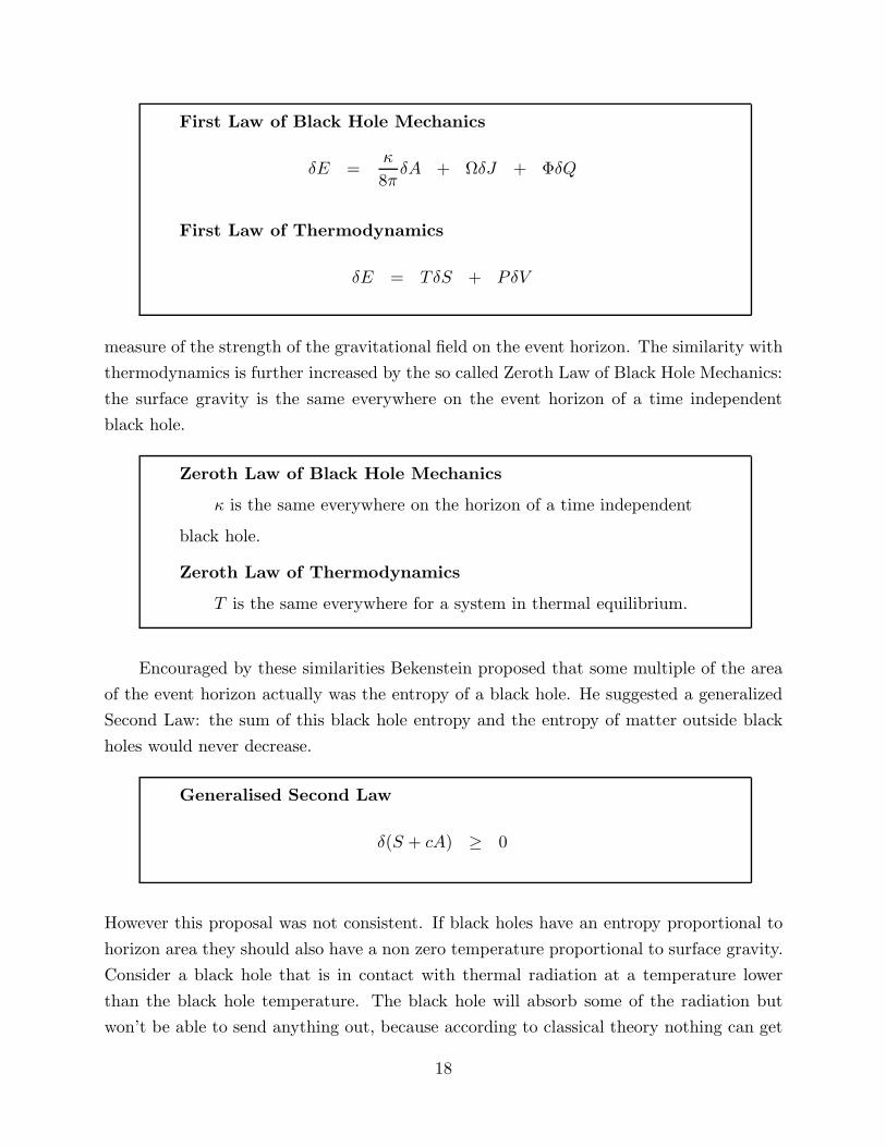
The similarity with thermodynamics is increased by what is called the First Law of

Black Hole Mechanics. This relates the change in mass of a black hole to the change in the

area of the event horizon and the change in its angular momentum and electric charge. One

can compare this to the First Law of Thermodynamics which gives the change in internal

energy in terms of the change in entropy and the external work done on the system.

One sees that if the area of the event horizon is analogous to entropy then the quantity

analogous to temperature is what is called the surface gravity of the black hole κ. This is a

17

First Law of Black Hole Mechanics

δE =κ

8πδA + ΩδJ + ΦδQ

First Law of Thermodynamics

δE = TδS + PδV

measure of the strength of the gravitational field on the event horizon. The similarity with

thermodynamics is further increased by the so called Zeroth Law of Black Hole Mechanics:

the surface gravity is the same everywhere on the event horizon of a time independent

black hole.

Zeroth Law of Black Hole Mechanics

κ is the same everywhere on the horizon of a time independent

black hole.

Zeroth Law of Thermodynamics

T is the same everywhere for a system in thermal equilibrium.

Encouraged by these similarities Bekenstein proposed that some multiple of the area

of the event horizon actually was the entropy of a black hole. He suggested a generalized

Second Law: the sum of this black hole entropy and the entropy of matter outside black

holes would never decrease.

Generalised Second Law

δ(S + cA) ≥ 0

However this proposal was not consistent. If black holes have an entropy proportional to

horizon area they should also have a non zero temperature proportional to surface gravity.

Consider a black hole that is in contact with thermal radiation at a temperature lower

than the black hole temperature. The black hole will absorb some of the radiation but

won’t be able to send anything out, because according to classical theory nothing can get

18

low temperaturethermal radiation

radiation being absorbedby black hole

black hole

out of a black hole. One thus has heat flow from the low temperature thermal radiation to

the higher temperature black hole. This would violate the generalized Second Law because

the loss of entropy from the thermal radiation would be greater than the increase in black

hole entropy. However, as we shall see in my next lecture, consistency was restored when

it was discovered that black holes are sending out radiation that was exactly thermal.

This is too beautiful a result to be a coincidence or just an approximation. So it seems

that black holes really do have intrinsic gravitational entropy. As I shall show, this is

related to the non trivial topology of a black hole. The intrinsic entropy means that

gravity introduces an extra level of unpredictability over and above the uncertainty usually

associated with quantum theory. So Einstein was wrong when he said “God does not play

dice”. Consideration of black holes suggests, not only that God does play dice, but that

He sometimes confuses us by throwing them where they can’t be seen.

19

20

2. Quantum Black Holes

S. W. Hawking

In my second lecture I’m going to talk about the quantum theory of black holes.

It seems to lead to a new level of unpredictability in physics over and above the usual

uncertainty associated with quantum mechanics. This is because black holes appear to

have intrinsic entropy and to lose information from our region of the universe. I should say

that these claims are controversial: many people working on quantum gravity, including

almost all those that entered it from particle physics, would instinctively reject the idea

that information about the quantum state of a system could be lost. However they have

had very little success in showing how information can get out of a black hole. Eventually

I believe they will be forced to accept my suggestion that it is lost, just as they were forced

to agree that black holes radiate, which was against all their preconceptions.

I should start by reminding you about the classical theory of black holes. We saw in

the last lecture that gravity is always attractive, at least in normal situations. If gravity

had been sometimes attractive and sometimes repulsive, like electro-dynamics, we would

never notice it at all because it is about 1040 times weaker. It is only because gravity always

has the same sign that the gravitational force between the particles of two macroscopic

bodies like ourselves and the Earth add up to give a force we can feel.

The fact that gravity is attractive means that it will tend to draw the matter in the

universe together to form objects like stars and galaxies. These can support themselves for

a time against further contraction by thermal pressure, in the case of stars, or by rotation

and internal motions, in the case of galaxies. However, eventually the heat or the angular

momentum will be carried away and the object will begin to shrink. If the mass is less

than about one and a half times that of the Sun the contraction can be stopped by the

degeneracy pressure of electrons or neutrons. The object will settle down to be a white

dwarf or a neutron star respectively. However, if the mass is greater than this limit there

is nothing that can hold it up and stop it continuing to contract. Once it has shrunk to a

certain critical size the gravitational field at its surface will be so strong that the light cones

will be bent inward as in the diagram on the following page. I would have liked to draw

you a four dimensional picture. However, government cuts have meant that Cambridge

university can afford only two dimensional screens. I have therefore shown time in the

vertical direction and used perspective to show two of the three space directions. You can

see that even the outgoing light rays are bent towards each other and so are converging

rather than diverging. This means that there is a closed trapped surface which is one of

the alternative third conditions of the Hawking-Penrose theorem.

21

r=0 singularity

trappedsurface

r = 2Mevent

horizon

surfaceof star

interiorof star

If the Cosmic Censorship Conjecture is correct the trapped surface and the singularity

it predicts can not be visible from far away. Thus there must be a region of spacetime

from which it is not possible to escape to infinity. This region is said to be a black hole.

Its boundary is called the event horizon and it is a null surface formed by the light rays

that just fail to get away to infinity. As we saw in the last lecture, the area of a cross

section of the event horizon can never decrease, at least in the classical theory. This, and

perturbation calculations of spherical collapse, suggest that black holes will settle down to

a stationary state. The no hair theorem, proved by the combined work of Israel, Carter,

Robinson and myself, shows that the only stationary black holes in the absence of matter

fields are the Kerr solutions. These are characterized by two parameters, the mass M and

the angular momentum J . The no hair theorem was extended by Robinson to the case

where there was an electromagnetic field. This added a third parameter Q, the electric

charge. The no hair theorem has not been proved for the Yang-Mills field, but the only

difference seems to be the addition of one or more integers that label a discrete family of

unstable solutions. It can be shown that there are no more continuous degrees of freedom

22

No Hair Theorem

Stationary black holes are characterised by mass M , angular

momentum J and electric charge Q.

of time independent Einstein-Yang-Mills black holes.

What the no hair theorems show is that a large amount of information is lost when

a body collapses to form a black hole. The collapsing body is described by a very large

number of parameters. There are the types of matter and the multipole moments of the

mass distribution. Yet the black hole that forms is completely independent of the type

of matter and rapidly loses all the multipole moments except the first two: the monopole

moment, which is the mass, and the dipole moment, which is the angular momentum.

This loss of information didn’t really matter in the classical theory. One could say that

all the information about the collapsing body was still inside the black hole. It would be

very difficult for an observer outside the black hole to determine what the collapsing body

was like. However, in the classical theory it was still possible in principle. The observer

would never actually lose sight of the collapsing body. Instead it would appear to slow

down and get very dim as it approached the event horizon. But the observer could still see

what it was made of and how the mass was distributed. However, quantum theory changed

all this. First, the collapsing body would send out only a limited number of photons before

it crossed the event horizon. They would be quite insufficient to carry all the information

about the collapsing body. This means that in quantum theory there’s no way an outside

observer can measure the state of the collapsed body. One might not think this mattered

23

too much because the information would still be inside the black hole even if one couldn’t

measure it from the outside. But this is where the second effect of quantum theory on

black holes comes in. As I will show, quantum theory will cause black holes to radiate

and lose mass. Eventually it seems that they will disappear completely, taking with them

the information inside them. I will give arguments that this information really is lost and

doesn’t come back in some form. As I will show, this loss of information would introduce a

new level of uncertainty into physics over and above the usual uncertainty associated with

quantum theory. Unfortunately, unlike Heisenberg’s Uncertainty Principle, this extra level

will be rather difficult to confirm experimentally in the case of black holes. But as I will

argue in my third lecture, there’s a sense in which we may have already observed it in the

measurements of fluctuations in the microwave background.

The fact that quantum theory causes black holes to radiate was first discovered by do-

ing quantum field theory on the background of a black hole formed by collapse. To see how

this comes about it is helpful to use what are normally called Penrose diagrams. However,

I think Penrose himself would agree they really should be called Carter diagrams because

Carter was the first to use them systematically. In a spherical collapse the spacetime won’t

depend on the angles θ and φ. All the geometry will take place in the r-t plane. Because

any two dimensional plane is conformal to flat space one can represent the causal structure

by a diagram in which null lines in the r-t plane are at ±45 degrees to the vertical.

centre ofsymmetry

r = 0

surfaces(t=constant)

two spheres(r=constant)

I +

I_

I 0

+(r =∞; t = +∞)

_(r =∞; t = _∞)

Let’s start with flat Minkowski space. That has a Carter-Penrose diagram which is a

triangle standing on one corner. The two diagonal sides on the right correspond to the

past and future null infinities I referred to in my first lecture. These are really at infinity

but all distances are shrunk by a conformal factor as one approaches past or future null

24

infinity. Each point of this triangle corresponds to a two sphere of radius r. r = 0 on the

vertical line on the left, which represents the center of symmetry, and r → ∞ on the right

of the diagram.

One can easily see from the diagram that every point in Minkowski space is in the

past of future null infinity I+. This means there is no black hole and no event horizon.

However, if one has a spherical body collapsing the diagram is rather different.

singularityevent horizon

collapsingbody

blackhole +

_

It looks the same in the past but now the top of the triangle has been cut off and replaced by

a horizontal boundary. This is the singularity that the Hawking-Penrose theorem predicts.

One can now see that there are points under this horizontal line that are not in the past

of future null infinity I+. In other words there is a black hole. The event horizon, the

boundary of the black hole, is a diagonal line that comes down from the top right corner

and meets the vertical line corresponding to the center of symmetry.

One can consider a scalar field φ on this background. If the spacetime were time

independent, a solution of the wave equation, that contained only positive frequencies on

scri minus, would also be positive frequency on scri plus. This would mean that there

would be no particle creation, and there would be no out going particles on scri plus, if

there were no scalar particles initially.

However, the metric is time dependent during the collapse. This will cause a solution

that is positive frequency on I− to be partly negative frequency when it gets to I+.

One can calculate this mixing by taking a wave with time dependence e−iωu on I+ and

propagating it back to I−. When one does that one finds that the part of the wave that

passes near the horizon is very blue shifted. Remarkably it turns out that the mixing is

independent of the details of the collapse in the limit of late times. It depends only on the

25

surface gravity κ that measures the strength of the gravitational field on the horizon of

the black hole. The mixing of positive and negative frequencies leads to particle creation.

When I first studied this effect in 1973 I expected I would find a burst of emission

during the collapse but that then the particle creation would die out and one would be

left with a black hole that was truely black. To my great surprise I found that after a

burst during the collapse there remained a steady rate of particle creation and emission.

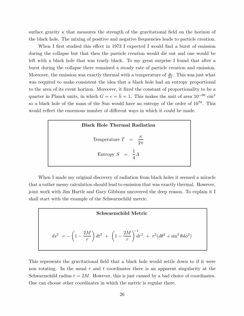
Moreover, the emission was exactly thermal with a temperature of κ2π

. This was just what

was required to make consistent the idea that a black hole had an entropy proportional

to the area of its event horizon. Moreover, it fixed the constant of proportionality to be a

quarter in Planck units, in which G = c = h = 1. This makes the unit of area 10−66 cm2

so a black hole of the mass of the Sun would have an entropy of the order of 1078. This

would reflect the enormous number of different ways in which it could be made.

Black Hole Thermal Radiation

Temperature T =κ

2π

Entropy S =1

4A

When I made my original discovery of radiation from black holes it seemed a miracle

that a rather messy calculation should lead to emission that was exactly thermal. However,

joint work with Jim Hartle and Gary Gibbons uncovered the deep reason. To explain it I

shall start with the example of the Schwarzschild metric.

Schwarzschild Metric

ds2 = −

(

1 −2M

r

)

dt2 +

(

1 −2M

r

)

−1

dr2 + r2(dθ2 + sin2 θdφ2)

This represents the gravitational field that a black hole would settle down to if it were

non rotating. In the usual r and t coordinates there is an apparent singularity at the

Schwarzschild radius r = 2M . However, this is just caused by a bad choice of coordinates.

One can choose other coordinates in which the metric is regular there.

26

r=0 singularity

r=0 singularity

future event horizon past event horizon

r = 2M

r=constant

1

2

3

4

I +

I_

I 0

+

_

The Carter-Penrose diagram has the form of a diamond with flattened top and bottom.

It is divided into four regions by the two null surfaces on which r = 2M . The region

on the right, marked ©1 on the diagram is the asymptotically flat space in which we are

supposed to live. It has past and future null infinities I− and I+ like flat spacetime. There

is another asymptotically flat region ©3 on the left that seems to correspond to another

universe that is connected to ours only through a wormhole. However, as we shall see, it

is connected to our region through imaginary time. The null surface from bottom left to

top right is the boundary of the region from which one can escape to the infinity on the

right. Thus it is the future event horizon. The epithet future being added to distinguish

it from the past event horizon which goes from bottom right to top left.

Let us now return to the Schwarzschild metric in the original r and t coordinates. If

one puts t = iτ one gets a positive definite metric. I shall refer to such positive definite

metrics as Euclidean even though they may be curved. In the Euclidean-Schwarzschild

metric there is again an apparent singularity at r = 2M . However, one can define a new

radial coordinate x to be 4M(1 − 2Mr−1)12 .

Euclidean-Schwarzschild Metric

ds2 = x2

(

dτ

4M

)2

+

(

r2

4M2

)2

dx2 + r2(dθ2 + sin2 θdφ2)

The metric in the x − τ plane then becomes like the origin of polar coordinates if one

identifies the coordinate τ with period 8πM . Similarly other Euclidean black hole metrics

will have apparent singularities on their horizons which can be removed by identifying the

27

r = constant

r=2M

2

periodτ = 8πΜ

τ = τ

1τ = τ

imaginary time coordinate with period 2πκ

.

So what is the significance of having imaginary time identified with some period β.

To see this consider the amplitude to go from some field configuration φ1 on the surface

t1 to a configuration φ2 on the surface t2. This will be given by the matrix element of

eiH(t2−t1). However, one can also represent this amplitude as a path integral over all fields

φ between t1 and t2 which agree with the given fields φ1 and φ2 on the two surfaces.

φ = φ2; t = t2

φ = φ1; t = t1

< φ2, t2 | φ1, t1 > = < φ2 | exp(−iH(t2 − t1)) | φ1 >

=

∫

D[φ] exp(iI[φ])

One now chooses the time separation (t2 − t1) to be pure imaginary and equal to β.

One also puts the initial field φ1 equal to the final field φ2 and sums over a complete basis

of states φn. On the left one has the expectation value of e−βH summed over all states.

This is just the thermodynamic partition function Z at the temperature T = β−1.

On the right hand of the equation one has a path integral. One puts φ1 = φ2 and

28

periodβ

t2 − t1 = −iβ, φ2 = φ1

Z =∑

< φn | exp(−βH) | φn >

=

∫

D[φ] exp(−iI [φ])

sums over all field configurations φn. This means that effectively one is doing the path

integral over all fields φ on a spacetime that is identified periodically in the imaginary

time direction with period β. Thus the partition function for the field φ at temperature

T is given by a path integral over all fields on a Euclidean spacetime. This spacetime is

periodic in the imaginary time direction with period β = T−1.

If one does the path integral in flat spacetime identified with period β in the imaginary

time direction one gets the usual result for the partition function of black body radiation.

However, as we have just seen, the Euclidean- Schwarzschild solution is also periodic in

imaginary time with period 2πκ

. This means that fields on the Schwarzschild background

will behave as if they were in a thermal state with temperature κ2π

.

The periodicity in imaginary time explained why the messy calculation of frequency

mixing led to radiation that was exactly thermal. However, this derivation avoided the

problem of the very high frequencies that take part in the frequency mixing approach.

It can also be applied when there are interactions between the quantum fields on the

background. The fact that the path integral is on a periodic background implies that all

physical quantities like expectation values will be thermal. This would have been very

difficult to establish in the frequency mixing approach.

One can extend these interactions to include interactions with the gravitational field

itself. One starts with a background metric g0 such as the Euclidean-Schwarzschild metric

that is a solution of the classical field equations. One can then expand the action I in a

power series in the perturbations δg about g0.

29

I[g] = I[g0] + I2(δg)2 + I3(δg)3 + ...

The linear term vanishes because the background is a solution of the field equations. The

quadratic term can be regarded as describing gravitons on the background while the cubic

and higher terms describe interactions between the gravitons. The path integral over

the quadratic terms are finite. There are non renormalizable divergences at two loops in

pure gravity but these cancel with the fermions in supergravity theories. It is not known

whether supergravity theories have divergences at three loops or higher because no one

has been brave or foolhardy enough to try the calculation. Some recent work indicates

that they may be finite to all orders. But even if there are higher loop divergences they

will make very little difference except when the background is curved on the scale of the

Planck length, 10−33 cm.

More interesting than the higher order terms is the zeroth order term, the action of

the background metric g0.

I = −1

16π

∫

R(−g)12 d4x +

1

8π

∫

K(±h)12 d3x

The usual Einstein-Hilbert action for general relativity is the volume integral of the scalar

curvature R. This is zero for vacuum solutions so one might think that the action of the

Euclidean-Schwarzschild solution was zero. However, there is also a surface term in the

action proportional to the integral of K, the trace of the second fundemental form of the

boundary surface. When one includes this and subtracts off the surface term for flat space

one finds the action of the Euclidean-Schwarzschild metric is β2

16πwhere β is the period in

imaginary time at infinity. Thus the dominant contribution to the path integral for the

partition function Z is e−β2

16π .

Z =∑

exp(−βEn) = exp

(

−β2

16π

)

If one differentiates log Z with respect to the period β one gets the expectation value

of the energy, or in other words, the mass.

< E >= −d

dβ(log Z) =

β

8π

So this gives the mass M = β8π

. This confirms the relation between the mass and the

period, or inverse temperature, that we already knew. However, one can go further. By

30

standard thermodynamic arguments, the log of the partition function is equal to minus

the free energy F divided by the temperature T .

log Z = −F

T

And the free energy is the mass or energy plus the temperature times the entropy S.

F = < E > + TS

Putting all this together one sees that the action of the black hole gives an entropy of

4πM2.

S =β2

16π= 4πM2 =

1

4A

This is exactly what is required to make the laws of black holes the same as the laws of

thermodynamics.

Why does one get this intrinsic gravitational entropy which has no parallel in other

quantum field theories. The reason is gravity allows different topologies for the spacetime

manifold.

IDE

NT

IFY

S1

S2

Boundary at infinity

In the case we are considering the Euclidean-Schwarzschild solution has a boundary at

infinity that has topology S2 × S1. The S2 is a large space like two sphere at infinity and

31

the S1 corresponds to the imaginary time direction which is identified periodically. One

can fill in this boundary with metrics of at least two different topologies. One of course

is the Euclidean-Schwarzschild metric. This has topology R2 × S2, that is the Euclidean

two plane times a two sphere. The other is R3 × S1, the topology of Euclidean flat space

periodically identified in the imaginary time direction. These two topologies have different

Euler numbers. The Euler number of periodically identified flat space is zero, while that

of the Euclidean-Schwarzschild solution is two.

surface term= 1

2 M (τ2_ τ1)

τ2

τ1volume term= 1

2 M (τ2_ τ1)

Total action = M(τ2 − τ1)

The significance of this is as follows: on the topology of periodically identified flat space

one can find a periodic time function τ whose gradient is no where zero and which agrees

with the imaginary time coordinate on the boundary at infinity. One can then work out

the action of the region between two surfaces τ1 and τ2. There will be two contributions

to the action, a volume integral over the matter Lagrangian, plus the Einstein-Hilbert

Lagrangian and a surface term. If the solution is time independent the surface term over

τ = τ1 will cancel with the surface term over τ = τ2. Thus the only net contribution

to the surface term comes from the boundary at infinity. This gives half the mass times

the imaginary time interval (τ2 − τ1). If the mass is non-zero there must be non-zero

matter fields to create the mass. One can show that the volume integral over the matter

Lagrangian plus the Einstein-Hilbert Lagrangian also gives 12M(τ2 − τ1). Thus the total

action is M(τ2 − τ1). If one puts this contribution to the log of the partition function into

the thermodynamic formulae one finds the expectation value of the energy to be the mass,

32

as one would expect. However, the entropy contributed by the background field will be

zero.

The situation is different however with the Euclidean-Schwarzschild solution.

τ = τ2

volume term = 0

fixed twosphere

r = 2M

surface term

= 12 M (τ2

_ τ1)

surface term from corner

= 12 M (τ2

_ τ1)

τ = τ1

Total action including corner contribution = M(τ2 − τ1)

Total action without corner contribution =1

2M(τ2 − τ1)

Because the Euler number is two rather than zero one can’t find a time function τ whose

gradient is everywhere non-zero. The best one can do is choose the imaginary time coor-

dinate of the Schwarzschild solution. This has a fixed two sphere at the horizon where τ

behaves like an angular coordinate. If one now works out the action between two surfaces

of constant τ the volume integral vanishes because there are no matter fields and the scalar

curvature is zero. The trace K surface term at infinity again gives 12M(τ2 − τ1). However

there is now another surface term at the horizon where the τ1 and τ2 surfaces meet in a

corner. One can evaluate this surface term and find that it also is equal to 12M(τ2 − τ1).

Thus the total action for the region between τ1 and τ2 is M(τ2−τ1). If one used this action

with τ2 − τ1 = β one would find that the entropy was zero. However, when one looks at

the action of the Euclidean Schwarzschild solution from a four dimensional point of view

rather than a 3+1, there is no reason to include a surface term on the horizon because the

metric is regular there. Leaving out the surface term on the horizon reduces the action by

one quarter the area of the horizon, which is just the intrinsic gravitational entropy of the

black hole.

The fact that the entropy of black holes is connected with a topological invariant,

the Euler number, is a strong argument that it will remain even if we have to go to a

33

more fundemental theory. This idea is anathema to most particle physicists who are a

very conservative lot and want to make everything like Yang-Mills theory. They agree that

the radiation from black holes seems to be thermal and independent of how the hole was

formed if the hole is large compared to the Planck length. But they would claim that when

the black hole loses mass and gets down to the Planck size, quantum general relativity will

break down and all bets will be off. However, I shall describe a thought experiment with

black holes in which information seems to be lost yet the curvature outside the horizons

always remains small.

It has been known for some time that one can create pairs of positively and negatively

charged particles in a strong electric field. One way of looking at this is to note that in

flat Euclidean space a particle of charge q such as an electron would move in a circle in a

uniform electric field E. One can analytically continue this motion from the imaginary time

τ to real time t. One gets a pair of positively and negatively charged particles accelerating

away from each other pulled apart by the electric field.

Electric Field

world line of electron

Euclidean space

Minkowski space

world lineof electron

world lineof positron

t = 0

τ = 0

The process of pair creation is described by chopping the two diagrams in half along

34

the t = 0 or τ = 0 lines. One then joins the upper half of the Minkowski space diagram to

the lower half of the Euclidean space diagram.

electron and positronaccelerating in electric

field

electron tunneling throughEuclidean space

Minkowski space

Euclidean space

This gives a picture in which the positively and negatively charged particles are really the

same particle. It tunnels through Euclidean space to get from one Minkowski space world

line to the other. To a first approximation the probability for pair creation is e−I where

Euclidean action I =2πm2

qE.

Pair creation by strong electric fields has been observed experimentally and the rate agrees

with these estimates.

Black holes can also carry electric charges so one might expect that they could also be

pair created. However the rate would be tiny compared to that for electron positron pairs

because the mass to charge ratio is 1020 times bigger. This means that any electric field

would be neutralized by electron positron pair creation long before there was a significant

probability of pair creating black holes. However there are also black hole solutions with

magnetic charges. Such black holes couldn’t be produced by gravitational collapse because

there are no magnetically charged elementary particles. But one might expect that they

could be pair created in a strong magnetic field. In this case there would be no competition

from ordinary particle creation because ordinary particles do not carry magnetic charges.

So the magnetic field could become strong enough that there was a significant chance of

creating a pair of magnetically charged black holes.

In 1976 Ernst found a solution that represented two magnetically charged black holes

accelerating away from each other in a magnetic field.

35

Lorentzian space

charged black holeaccelerating in magnetic field

t = 0

black hole

Euclidean space

τ = 0

If one analytically continues it to imaginary time one has a picture very like that of the

electron pair creation. The black hole moves on a circle in a curved Euclidean space just

like the electron moves in a circle in flat Euclidean space. There is a complication in the

black hole case because the imaginary time coordinate is periodic about the horizon of the

black hole as well as about the center of the circle on which the black hole moves. One has

to adjust the mass to charge ratio of the black hole to make these periods equal. Physically

this means that one chooses the parameters of the black hole so that the temperature of the

black hole is equal to the temperature it sees because it is accelerating.. The temperature

of a magnetically charged black hole tends to zero as the charge tends to the mass in

Planck units. Thus for weak magnetic fields, and hence low acceleration, one can always

match the periods.

Like in the case of pair creation of electrons one can describe pair creation of black

holes by joining the lower half of the imaginary time Euclidean solution to the upper half

of the real time Lorentzian solution.

One can think of the black hole as tunneling through the Euclidean region and emerging

as a pair of oppositely charged black holes that accelerate away from each other pulled

36

black holeaccelerating

black hole tunneling throughEuclidean space

Lorentzian space

Euclidean space

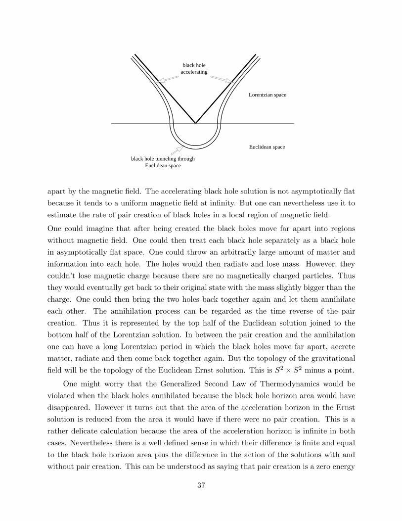
apart by the magnetic field. The accelerating black hole solution is not asymptotically flat

because it tends to a uniform magnetic field at infinity. But one can nevertheless use it to

estimate the rate of pair creation of black holes in a local region of magnetic field.

One could imagine that after being created the black holes move far apart into regions

without magnetic field. One could then treat each black hole separately as a black hole

in asymptotically flat space. One could throw an arbitrarily large amount of matter and

information into each hole. The holes would then radiate and lose mass. However, they

couldn’t lose magnetic charge because there are no magnetically charged particles. Thus

they would eventually get back to their original state with the mass slightly bigger than the

charge. One could then bring the two holes back together again and let them annihilate

each other. The annihilation process can be regarded as the time reverse of the pair

creation. Thus it is represented by the top half of the Euclidean solution joined to the

bottom half of the Lorentzian solution. In between the pair creation and the annihilation

one can have a long Lorentzian period in which the black holes move far apart, accrete

matter, radiate and then come back together again. But the topology of the gravitational

field will be the topology of the Euclidean Ernst solution. This is S2 × S2 minus a point.

One might worry that the Generalized Second Law of Thermodynamics would be

violated when the black holes annihilated because the black hole horizon area would have

disappeared. However it turns out that the area of the acceleration horizon in the Ernst

solution is reduced from the area it would have if there were no pair creation. This is a

rather delicate calculation because the area of the acceleration horizon is infinite in both

cases. Nevertheless there is a well defined sense in which their difference is finite and equal

to the black hole horizon area plus the difference in the action of the solutions with and

without pair creation. This can be understood as saying that pair creation is a zero energy

37

black hole tunneling throughEuclidean space to pair create

Lorentzian space

Euclidean space

Euclidean space

black hole tunneling throughEuclidean space to annihilate

matter and informationthrown into black hole

which radiates

process; the Hamiltonian with pair creation is the same as the Hamiltonian without. I’m

very grateful to Simon Ross and Gary Horovitz for calculating this reduction just in time

for this lecture. It is miracles like this, and I mean the result not that they got it, that

convince me that black hole thermodynamics can’t just be a low energy approximation.

I believe that gravitational entropy won’t disappear even if we have to go to a more

fundemental theory of quantum gravity.

One can see from this thought experiment that one gets intrinsic gravitational en-

tropy and loss of information when the topology of spacetime is different from that of flat

Minkowski space. If the black holes that pair create are large compared to the Planck

size the curvature outside the horizons will be everywhere small compared to the Planck

scale. This means the approximation I have made of ignoring cubic and higher terms in

the perturbations should be good. Thus the conclusion that information can be lost in

black holes should be reliable.

38

If information is lost in macroscopic black holes it should also be lost in processes

in which microscopic, virtual black holes appear because of quantum fluctuations of the

metric. One could imagine that particles and information could fall into these holes and

get lost. Maybe that is where all those odd socks went. Quantities like energy and electric

charge, that are coupled to gauge fields, would be conserved but other information and

global charge would be lost. This would have far reaching implications for quantum theory.

It is normally assumed that a system in a pure quantum state evolves in a unitary way

through a succession of pure quantum states. But if there is loss of information through the

appearance and disappearance of black holes there can’t be a unitary evolution. Instead

the loss of information will mean that the final state after the black holes have disappeared

will be what is called a mixed quantum state. This can be regarded as an ensemble of

different pure quantum states each with its own probability. But because it is not with

certainty in any one state one can not reduce the probability of the final state to zero

by interfering with any quantum state. This means that gravity introduces a new level

of unpredictability into physics over and above the uncertainty usually associated with

quantum theory. I shall show in the next lecture we may have already observed this extra

uncertainty. It means an end to the hope of scientific determinism that we could predict

the future with certainty. It seems God still has a few tricks up his sleeve.

A

A

A

A

A

A

A

A

39

3. Quantum Cosmology

S. W. Hawking

In my third lecture I shall turn to cosmology. Cosmology used to be considered a

pseudo-science and the preserve of physicists who may have done useful work in their

earlier years but who had gone mystic in their dotage. There were two reasons for this.

The first was that there was an almost total absence of reliable observations. Indeed,

until the 1920s about the only important cosmological observation was that the sky at

night is dark. But people didn’t appreciate the significance of this. However, in recent

years the range and quality of cosmological observations has improved enormously with

developments in technology. So this objection against regarding cosmology as a science,

that it doesn’t have an observational basis is no longer valid.

There is, however, a second and more serious objection. Cosmology can not predict

anything about the universe unless it makes some assumption about the initial conditions.

Without such an assumption, all one can say is that things are as they are now because

they were as they were at an earlier stage. Yet many people believe that science should be

concerned only with the local laws which govern how the universe evolves in time. They

would feel that the boundary conditions for the universe that determine how the universe

began were a question for metaphysics or religion rather than science.

The situation was made worse by the theorems that Roger and I proved. These

showed that according to general relativity there should be a singularity in our past. At

this singularity the field equations could not be defined. Thus classical general relativity

brings about its own downfall: it predicts that it can’t predict the universe.

Although many people welcomed this conclusion, it has always profoundly disturbed

me. If the laws of physics could break down at the begining of the universe, why couldn’t

they break down any where. In quantum theory it is a principle that anything can happen if

it is not absolutely forbidden. Once one allows that singular histories could take part in the

path integral they could occur any where and predictability would disappear completely.

If the laws of physics break down at singularities, they could break down any where.

The only way to have a scientific theory is if the laws of physics hold everywhere

including at the begining of the universe. One can regard this as a triumph for the

principles of democracy: Why should the begining of the universe be exempt from the

laws that apply to other points. If all points are equal one can’t allow some to be more

equal than others.

To implement the idea that the laws of physics hold everywhere, one should take the

path integral only over non-singular metrics. One knows in the ordinary path integral case

40

that the measure is concentrated on non-differentiable paths. But these are the completion

in some suitable topology of the set of smooth paths with well defined action. Similarly,

one would expect that the path integral for quantum gravity should be taken over the

completion of the space of smooth metrics. What the path integral can’t include is metrics

with singularities whose action is not defined.

In the case of black holes we saw that the path integral should be taken over Euclidean,

that is, positive definite metrics. This meant that the singularities of black holes, like the

Schwarzschild solution, did not appear on the Euclidean metrics which did not go inside

the horizon. Instead the horizon was like the origin of polar coordinates. The action of the

Euclidean metric was therefore well defined. One could regard this as a quantum version

of Cosmic Censorship: the break down of the structure at a singularity should not affect

any physical measurement.

It seems, therefore, that the path integral for quantum gravity should be taken over

non-singular Euclidean metrics. But what should the boundary conditions be on these

metrics. There are two, and only two, natural choices. The first is metrics that approach

the flat Euclidean metric outside a compact set. The second possibility is metrics on

manifolds that are compact and without boundary.

Natural choices for path integral for quantum gravity

1. Asymptotically Euclidean metrics.

2. Compact metrics without boundary.

The first class of asymptotically Euclidean metrics is obviously appropriate for scat-

tering calculations.

interactionregion

particles comingin from infinity

particles goingout to infinity

41

In these one sends particles in from infinity and observes what comes out again to infinity.

All measurements are made at infinity where one has a flat background metric and one

can interpret small fluctuations in the fields as particles in the usual way. One doesn’t

ask what happens in the interaction region in the middle. That is why one does a path

integral over all possible histories for the interaction region, that is, over all asymptotically

Euclidean metrics.

However, in cosmology one is interested in measurements that are made in a finite

region rather than at infinity. We are on the inside of the universe not looking in from the

outside. To see what difference this makes let us first suppose that the path integral for

cosmology is to be taken over all asymptotically Euclidean metrics.

Connected asymptotically Euclidean metric

Disconnected asymptotically Euclidean metric

compactmetric

region ofmeasurement

asymptoticallyEuclidean metric

region ofmeasurement

asymptoticallyEuclidean metric

Then there would be two contributions to probabilities for measurements in a finite region.

The first would be from connected asymptotically Euclidean metrics. The second would

be from disconnected metrics that consisted of a compact spacetime containing the region

of measurements and a separate asymptotically Euclidean metric. One can not exclude

disconnected metrics from the path integral because they can be approximated by con-

42

nected metrics in which the different components are joined by thin tubes or wormholes

of neglible action.

Disconnected compact regions of spacetime won’t affect scattering calculations be-

cause they aren’t connected to infinity, where all measurements are made. But they will

affect measurements in cosmology that are made in a finite region. Indeed, the contribu-

tions from such disconnected metrics will dominate over the contributions from connected

asymptotically Euclidean metrics. Thus, even if one took the path integral for cosmology

to be over all asymptotically Euclidean metrics, the effect would be almost the same as if

the path integral had been over all compact metrics. It therefore seems more natural to

take the path integral for cosmology to be over all compact metrics without boundary, as

Jim Hartle and I proposed in 1983.

The No Boundary Proposal (Hartle and Hawking)

The path integral for quantum gravity should be taken over all compact

Euclidean metrics.

One can paraphrase this as The Boundary Condition Of The Universe Is That It Has No

Boundary.

In the rest of this lecture I shall show that this no boundary proposal seems to account

for the universe we live in. That is an isotropic and homogeneous expanding universe with

small perturbations. We can observe the spectrum and statistics of these perturbations in

the fluctuations in the microwave background. The results so far agree with the predictions

of the no boundary proposal. It will be a real test of the proposal and the whole Euclidean

quantum gravity program when the observations of the microwave background are extended

to smaller angular scales.

In order to use the no boundary proposal to make predictions, it is useful to introduce

a concept that can describe the state of the universe at one time.

Consider the probability that the spacetime manifold M contains an embedded three

dimensional manifold Σ with induced metric hij . This is given by a path integral over all

metrics gab on M that induce hij on Σ. If M is simply connected, which I will assume,

the surface Σ will divide M into two parts M+ and M−.

In this case, the probability for Σ to have the metric hij can be factorized. It is the product

of two wave functions Ψ+ and Ψ−. These are given by path integrals over all metrics on

M+ and M− respectively, that induce the given three metric hij on Σ. In most cases, the

two wave functions will be equal and I will drop the superscripts + and −. Ψ is called

43

M +

M_

Σ

Probability of induced metric hij on Σ =

∫

metrics on M that

induce hij on Σ

d[g] e−I

M +

Σ

Probability of hij = Ψ+(hij) × Ψ−(hij)

where Ψ+(hij) =

∫

metrics on M+ that

induce hij on Σ

d[g] e−I

the wave function of the universe. If there are matter fields φ, the wave function will also

depend on their values φ0 on Σ. But it will not depend explicitly on time because there

is no preferred time coordinate in a closed universe. The no boundary proposal implies

that the wave function of the universe is given by a path integral over fields on a compact

manifold M+ whose only boundary is the surface Σ. The path integral is taken over all

metrics and matter fields on M+ that agree with the metric hij and matter fields φ0 on

Σ.

One can describe the position of the surface Σ by a function τ of three coordinates xi

on Σ. But the wave function defined by the path integral can’t depend on τ or on the choice

44

of the coordinates xi. This implies that the wave function Ψ has to obey four functional

differential equations. Three of these equations are called the momentum constraints.

Momentum Constraint Equation

(

∂Ψ

∂hij

)

;j

= 0

They express the fact that the wave function should be the same for different 3 metrics

hij that can be obtained from each other by transformations of the coordinates xi. The

fourth equation is called the Wheeler-DeWitt equation.

Wheeler - DeWitt Equation

(

Gijkl

∂2

∂hij∂hkl

− h12

3R

)

Ψ = 0

It corresponds to the independence of the wave function on τ . One can think of it as the

Schrodinger equation for the universe. But there is no time derivative term because the

wave function does not depend on time explicitly.

In order to estimate the wave function of the universe, one can use the saddle point

approximation to the path integral as in the case of black holes. One finds a Euclidean

metric g0 on the manifold M+ that satisfies the field equations and induces the metric

hij on the boundary Σ. One can then expand the action in a power series around the

background metric g0.

I[g] = I[g0] +1

2δgI2δg + ...

As before the term linear in the perturbations vanishes. The quadratic term can be re-

garded as giving the contribution of gravitons on the background and the higher order

terms as interactions between the gravitons. These can be ignored when the radius of

curvature of the background is large compared to the Planck scale. Therefore

Ψ ≈1

(det I2)12

e−I[go]

45

action = _ 1Λ

1 _ 1 _ Λ3

a2

32

M +

Σ3-sphereof radius a

radiusH

=3

Λ

M +

Σ

14−sphere of

action = _ 1Λ

1 + 1 _ Λ3

a2

32 ( ) ( )

One can see what the wave function is like from a simple example. Consider a situation

in which there are no matter fields but there is a positive cosmological constant Λ.

Let us take the surface Σ to be a three sphere and the metric hij to be the round three

sphere metric of radius a. Then the manifold M+ bounded by Σ can be taken to be the

four ball. The metric that satisfies the field equations is part of a four sphere of radius 1H

where H2 = Λ3 .

I =1

16π

∫

(R − 2Λ)(−g)12 d4x +

1

8π

∫

K(±h)12 d3x

For a three sphere Σ of radius less than 1H

there are two possible Euclidean solutions:

either M+ can be less than a hemisphere or it can be more. However there are arguments

that show that one should pick the solution corresponding to less than a hemisphere.

The next figure shows the contribution to the wave function that comes from the

action of the metric g0. When the radius of Σ is less than 1H

the wave function increases

exponentially like ea2

. However, when a is greater than 1H

one can analytically continue

the result for smaller a and obtain a wave function that oscillates very rapidly.

One can interpret this wave function as follows. The real time solution of the Einstein

equations with a Λ term and maximal symmetry is de Sitter space. This can be embedded

as a hyperboloid in five dimensional Minkowski space.

One can think of it as a closed universe that shrinks down from infinite size to a minimum

radius and then expands again exponentially. The metric can be written in the form of a

Friedmann universe with scale factor coshHt. Putting τ = it converts the cosh into cos

giving the Euclidean metric on a four sphere of radius 1H

.

46

Ψ

a1H

=3Λ

Euclidean4-sphere

Lorentziande Sitter space

maximumradius =

minimumradius

=3Λ

3Λ

Lorentzian - de Sitter Metric

ds2 = −dt2 +1

H2coshHt(dr2 + sin2 r(dθ2 + sin2 θdφ2))

Thus one gets the idea that a wave function which varies exponentially with the three

metric hij corresponds to an imaginary time Euclidean metric. On the other hand, a wave

function which oscillates rapidly corresponds to a real time Lorentzian metric.

Like in the case of the pair creation of black holes, one can describe the spontaneous

creation of an exponentially expanding universe. One joins the lower half of the Euclidean

four sphere to the upper half of the Lorentzian hyperboloid.

47

Euclidean Metric

ds2 = dτ2 +1

H2cos Hτ(dr2 + sin2 r(dθ2 + sin2 θdφ2))

Lorentziande Sitter solution

Euclidean4-sphere

Unlike the black hole pair creation, one couldn’t say that the de Sitter universe was created

out of field energy in a pre-existing space. Instead, it would quite literally be created out

of nothing: not just out of the vacuum but out of absolutely nothing at all because there

is nothing outside the universe. In the Euclidean regime, the de Sitter universe is just a

closed space like the surface of the Earth but with two more dimensions. If the cosmological

constant is small compared to the Planck value, the curvature of the Euclidean four sphere

should be small. This will mean that the saddle point approximation to the path integral

should be good, and that the calculation of the wave function of the universe won’t be

affected by our ignorance of what happens in very high curvatures.

One can also solve the field equations for boundary metrics that aren’t exactly the

round three sphere metric. If the radius of the three sphere is less than 1H

, the solution is a

real Euclidean metric. The action will be real and the wave function will be exponentially

damped compared to the round three sphere of the same volume. If the radius of the three

sphere is greater than this critical radius there will be two complex conjugate solutions

and the wave function will oscillate rapidly with small changes in hij .

Any measurement made in cosmology can be formulated in terms of the wave function.

48

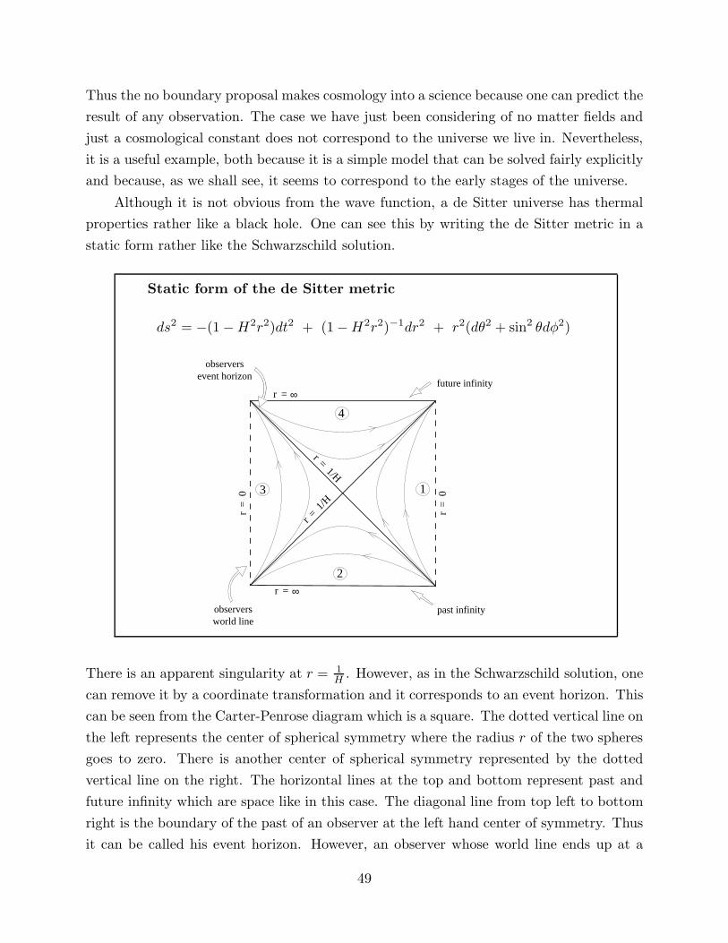
Thus the no boundary proposal makes cosmology into a science because one can predict the

result of any observation. The case we have just been considering of no matter fields and

just a cosmological constant does not correspond to the universe we live in. Nevertheless,

it is a useful example, both because it is a simple model that can be solved fairly explicitly

and because, as we shall see, it seems to correspond to the early stages of the universe.

Although it is not obvious from the wave function, a de Sitter universe has thermal

properties rather like a black hole. One can see this by writing the de Sitter metric in a

static form rather like the Schwarzschild solution.

Static form of the de Sitter metric

ds2 = −(1 − H2r2)dt2 + (1 − H2r2)−1dr2 + r2(dθ2 + sin2 θdφ2)

r = ∞

r =1/

H

r=

0

r = ∞

r =1/H

r=

0 3

4

1

2

observersworld line

observersevent horizon

past infinity

future infinity

There is an apparent singularity at r = 1H

. However, as in the Schwarzschild solution, one

can remove it by a coordinate transformation and it corresponds to an event horizon. This

can be seen from the Carter-Penrose diagram which is a square. The dotted vertical line on

the left represents the center of spherical symmetry where the radius r of the two spheres

goes to zero. There is another center of spherical symmetry represented by the dotted

vertical line on the right. The horizontal lines at the top and bottom represent past and

future infinity which are space like in this case. The diagonal line from top left to bottom

right is the boundary of the past of an observer at the left hand center of symmetry. Thus

it can be called his event horizon. However, an observer whose world line ends up at a

49

different place on future infinity will have a different event horizon. Thus event horizons

are a personal matter in de Sitter space.

If one returns to the static form of the de Sitter metric and put τ = it one gets a

Euclidean metric. There is an apparent singularity on the horizon. However, by defining

a new radial coordinate and identifying τ with period 2πH

, one gets a regular Euclidean

metric which is just the four sphere. Because the imaginary time coordinate is periodic, de

Sitter space and all quantum fields in it will behave as if they were at a temperature H2π

.

As we shall see, we can observe the consequences of this temperature in the fluctuations in

the microwave background. One can also apply arguments similar to the black hole case

to the action of the Euclidean-de Sitter solution. One finds that it has an intrinsic entropy

of πH2 , which is a quarter of the area of the event horizon. Again this entropy arises for

a topological reason: the Euler number of the four sphere is two. This means that there

can not be a global time coordinate on Euclidean-de Sitter space. One can interpret this

cosmological entropy as reflecting an observers lack of knowledge of the universe beyond

his event horizon.

Euclidean metric periodic with period2π

H

⇒

Temperature = H2π

Area of event horizon = 4πH2

Entropy = πH2

De Sitter space is not a good model of the universe we live in because it is empty and

it is expanding exponentially. We observe that the universe contains matter and we deduce

from the microwave background and the abundances of light elements that it must have

been much hotter and denser in the past. The simplest scheme that is consistent with our

observations is called the Hot Big Bang model.

In this scenario, the universe starts at a singularity filled with radiation at an infinite tem-

perature. As it expands, the radiation cools and its energy density goes down. Eventually

the energy density of the radiation becomes less than the density of non relativistic matter

which has dominated over the expansion by the last factor of a thousand. However we

can still observe the remains of the radiation in a background of microwave radiation at a

temperature of about 3 degrees above absolute zero.

The trouble with the Hot Big Bang model is the trouble with all cosmology without

a theory of initial conditions: it has no predictive power. Because general relativity would

50

Hot Big Bang Model

radius ofthe universe

temperatureof the universe

radius/

time

temperature

break down at a singularity, anything could come out of the Big Bang. So why is the

universe so homogeneous and isotropic on a large scale yet with local irregularities like

galaxies and stars. And why is the universe so close to the dividing line between collapsing

again and expanding indefinitely. In order to be as close as we are now the rate of expansion

early on had to be chosen fantastically accurately. If the rate of expansion one second after

the Big Bang had been less by one part in 1010, the universe would have collapsed after

a few million years. If it had been greater by one part in 1010, the universe would have

been essentially empty after a few million years. In neither case would it have lasted long

enough for life to develop. Thus one either has to appeal to the anthropic principle or find

some physical explanation of why the universe is the way it is.

Hot Big Bang model does not explain why :

1. The universe is nearly homogeneous and isotropic but with small pertur-

bations.

2. The universe is expanding at almost exactly the critical rate to avoid col-

lapsing again.

Some people have claimed that what is called inflation removes the need for a theory

of initial conditions. The idea is that the universe could start out at the the Big Bang in

almost any state. In those parts of the universe in which conditions were suitable there

would be a period of exponential expansion called inflation. Not only could this increase

the size of the region by an enormous factor like 1030 or more, it would also leave the region

homogeneous and isotropic and expanding at just the critical rate to avoid collapsing again.

The claim would be that intelligent life would develop only in regions that inflated. We

51

should not, therefore, be surprised that our region is homogeneous and isotropic and is

expanding at just the critical rate.

However, inflation alone can not explain the present state of the universe. One can

see this by taking any state for the universe now and running it back in time. Providing it

contains enough matter, the singularity theorems will imply that there was a singularity

in the past. One can choose the initial conditions of the universe at the Big Bang to be the

initial conditions of this model. In this way, one can show that arbitrary initial conditions

at the Big Bang can lead to any state now. One can’t even argue that most initial states

lead to a state like we observe today: the natural measure of both the initial conditions

that do lead to a universe like ours and those that don’t is infinite. One can’t therefore

claim that one is bigger than the other.

On the other hand, we saw in the case of gravity with a cosmological constant but no

matter fields that the no boundary condition could lead to a universe that was predictable

within the limits of quantum theory. This particular model did not describe the universe

we live in, which is full of matter and has zero or very small cosmological constant. However

one can get a more realistic model by dropping the cosmological constant and including

matter fields. In particular, one seems to need a scalar field φ with potential V (φ). I shall

assume that V has a minimum value of zero at φ = 0. A simple example would be a

massive scalar field V = 12m2φ2.

φ

V(φ)

Energy - Momentum Tensor of a Scalar Field

Tab = φ,aφ,b −1

2gabφ,cφ

,c − gabV (φ)

52

One can see from the energy momentum tensor that if the gradient of φ is small V (φ) acts

like an effective cosmological constant.

The wave function will now depend on the value φ0 of φ on Σ, as well as on the induced

metric hij . One can solve the field equations for small round three sphere metrics and large

values of φ0. The solution with that boundary is approximately part of a four sphere and

a nearly constant φ field. This is like the de Sitter case with the potential V (φ0) playing

the role of the cosmological constant. Similarly, if the radius a of the three sphere is a bit

bigger than the radius of the Euclidean four sphere there will be two complex conjugate

solutions. These will be like half of the Euclidean four sphere joined onto a Lorentzian-

de Sitter solution with almost constant φ. Thus the no boundary proposal predicts the

spontaneous creation of an exponentially expanding universe in this model as well as in

the de Sitter case.

One can now consider the evolution of this model. Unlike the de Sitter case, it will not

continue indefinitely with exponential expansion. The scalar field will run down the hill of

the potential V to the minimum at φ = 0. However, if the initial value of φ is larger than

the Planck value, the rate of roll down will be slow compared to the expansion time scale.

Thus the universe will expand almost exponentially by a large factor. When the scalar

field gets down to order one, it will start to oscillate about φ = 0. For most potentials V ,

the oscillations will be rapid compared to the expansion time. It is normally assumed that

the energy in these scalar field oscillations will be converted into pairs of other particles

and will heat up the universe. This, however, depends on an assumption about the arrow

of time. I shall come back to this shortly.

The exponential expansion by a large factor would have left the universe with almost

exactly the critical rate of expansion. Thus the no boundary proposal can explain why

the universe is still so close to the critical rate of expansion. To see what it predicts

for the homogeneity and isotropy of the universe, one has to consider three metrics hij

which are perturbations of the round three sphere metric. One can expand these in terms

of spherical harmonics. There are three kinds: scalar harmonics, vector harmonics and

tensor harmonics. The vector harmonics just correspond to changes of the coordinates xi

on successive three spheres and play no dynamical role. The tensor harmonics correspond

to gravitational waves in the expanding universe, while the scalar harmonics correspond

partly to coordinate freedom and partly to density perturbations.

One can write the wave function Ψ as a product of a wave function Ψ0 for a round

three sphere metric of radius a times wave functions for the coefficients of the harmonics.

Ψ[hij , φ0] = Ψ0(a, φ)Ψa(an)Ψb(bn)Ψc(cn)Ψd(dn)

53

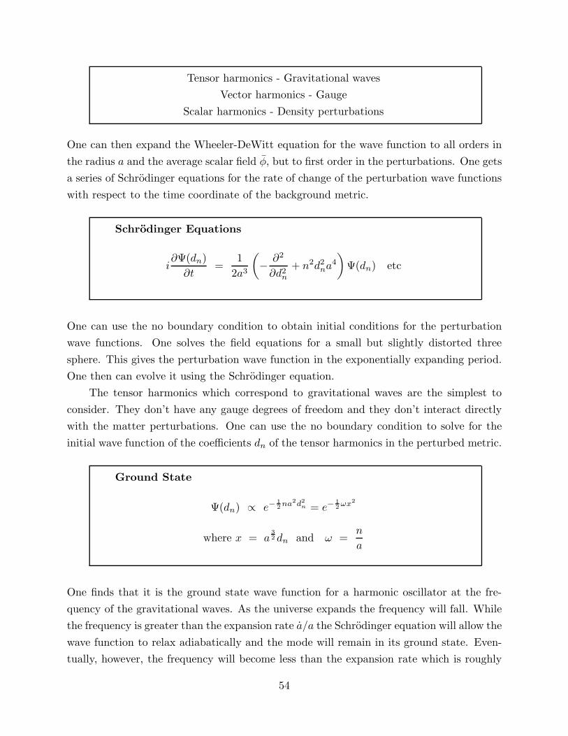
Tensor harmonics - Gravitational waves

Vector harmonics - Gauge

Scalar harmonics - Density perturbations

One can then expand the Wheeler-DeWitt equation for the wave function to all orders in

the radius a and the average scalar field φ, but to first order in the perturbations. One gets

a series of Schrodinger equations for the rate of change of the perturbation wave functions

with respect to the time coordinate of the background metric.

Schrodinger Equations

i∂Ψ(dn)

∂t=

1

2a3

(

−∂2

∂d2n

+ n2d2na4

)

Ψ(dn) etc

One can use the no boundary condition to obtain initial conditions for the perturbation

wave functions. One solves the field equations for a small but slightly distorted three

sphere. This gives the perturbation wave function in the exponentially expanding period.

One then can evolve it using the Schrodinger equation.

The tensor harmonics which correspond to gravitational waves are the simplest to

consider. They don’t have any gauge degrees of freedom and they don’t interact directly

with the matter perturbations. One can use the no boundary condition to solve for the

initial wave function of the coefficients dn of the tensor harmonics in the perturbed metric.

Ground State

Ψ(dn) ∝ e−12na2d2

n = e−12ωx2

where x = a32 dn and ω =

n

a

One finds that it is the ground state wave function for a harmonic oscillator at the fre-

quency of the gravitational waves. As the universe expands the frequency will fall. While

the frequency is greater than the expansion rate a/a the Schrodinger equation will allow the

wave function to relax adiabatically and the mode will remain in its ground state. Even-

tually, however, the frequency will become less than the expansion rate which is roughly

54

constant during the exponential expansion. When this happens the Schrodinger equation

will no longer be able to change the wave function fast enough that it can remain in the

ground state while the frequency changes. Instead it will freeze in the shape it had when

the frequency fell below the expansion rate.

wavelength/

time

radius

wave function frozen

end ofinflation

adiabaticevolution

perturbationscome back within

horizon radius

perturbation becomes greaterthan the horizon radius

wavelength of perturbations

horizon radius

After the end of the exponential expansion era, the expansion rate will decrease faster

than the frequency of the mode. This is equivalent to saying that an observers event

horizon, the reciprocal of the expansion rate, increases faster than the wave length of the

mode. Thus the wave length will get longer than the horizon during the inflation period

and will come back within the horizon later on. When it does, the wave function will still

be the same as when the wave function froze. The frequency, however, will be much lower.

The wave function will therefore correspond to a highly excited state rather than to the

ground state as it did when the wave function froze. These quantum excitations of the

gravitational wave modes will produce angular fluctuations in the microwave background

whose amplitude is the expansion rate (in Planck units) at the time the wave function

froze. Thus the COBE observations of fluctuations of one part in 105 in the microwave

background place an upper limit of about 10−10 in Planck units on the energy density

when the wave function froze. This is sufficiently low that the approximations I have used

should be accurate.

However, the gravitational wave tensor harmonics give only an upper limit on the

density at the time of freezing. The reason is that it turns out that the scalar harmonics

give a larger fluctuation in the microwave background. There are two scalar harmonic

55

degrees of freedom in the three metric hij and one in the scalar field. However two of these

scalar degrees correspond to coordinate freedom. Thus there is only one physical scalar

degree of freedom and it corresponds to density perturbations.

The analysis for the scalar perturbations is very similar to that for the tensor harmon-

ics if one uses one coordinate choice for the period up to the wave function freezing and

another after that. In converting from one coordinate system to the other, the amplitudes

get multiplied by a factor of the expansion rate divided by the average rate of change

of phi. This factor will depend on the slope of the potential, but will be at least 10 for

reasonable potentials. This means the fluctuations in the microwave background that the

density perturbations produce will be at least 10 times bigger than from the gravitational

waves. Thus the upper limit on the energy density at the time of wave function freezing

is only 10−12 of the Planck density. This is well within the range of the validity of the

approximations I have been using. Thus it seems we don’t need string theory even for the

beginning of the universe.

The spectrum of the fluctuations with angular scale agrees within the accuracy of the

present observations with the prediction that it should be almost scale free. And the size

of the density perturbations is just that required to explain the formation of galaxies and

stars. Thus it seems the no boundary proposal can explain all the structure of the universe

including little inhomogeneities like ourselves.

One can think of the perturbations in the microwave background as arising from

thermal fluctuations in the scalar field φ. The inflationary period has a temperature

of the expansion rate over 2π because it is approximately periodic in imaginary time.

Thus, in a sense, we don’t need to find a little primordial black hole: we have already

observed an intrinsic gravitational temperature of about 1026 degrees, or 10−6 of the Planck

temperature.

COBE predictions plus

gravitational wave perturbations⇒

upper limit on energy density

10−10 Planck density

plus density perturbations ⇒upper limit on energy density

10−12 Planck density

intrinsic gravitational

temperature of early universe≈

10−6 Planck temperature

= 1026 degrees

What about the intrinsic entropy associated with the cosmological event horizon. Can

56

we observe this. I think we can and that it corresponds to the fact that objects like galaxies

and stars are classical objects even though they are formed by quantum fluctuations. If one

looks at the universe on a space like surface Σ that spans the whole universe at one time,

then it is in a single quantum state described by the wave function Ψ. However, we can

never see more than half of Σ and we are completely ignorant of what the universe is like

beyond our past light cone. This means that in calculating the probability for observations,

we have to sum over all possibilities for the part of Σ we don’t observe. The effect of

the summation is to change the part of the universe we observe from a single quantum

state to what is called a mixed state, a statistical ensemble of different possibilities. Such

decoherence, as it is called, is necessary if a system is to behave in a classical manner rather

than a quantum one. People normally try to account for decoherence by interactions with

an external system, such as a heat bath, that is not measured. In the case of the universe

there is no external system, but I would suggest that the reason we observe classical

behavior is that we can see only part of the universe. One might think that at late times

one would be able to see all the universe and the event horizon would disappear. But this

is not the case. The no boundary proposal implies that the universe is spatially closed. A

closed universe will collapse again before an observer has time to see all the universe. I

have tried to show the entropy of such a universe would be a quarter of the area of the

event horizon at the time of maximum expansion. However, at the moment, I seem to be

getting a factor of 316 rather than a 1

4 . Obviously I’m either on the wrong track or I’m

missing something.

I will end this lecture on a topic on which Roger and I have very different views,

the arrow of time. There is a very clear distinction between the forward and backward

directions of time in our region of the universe. One only has to watch a film being run

backwards to see the difference. Instead of cups falling off tables and getting broken, they

would mend themselves and jump back on the table. If only real life were like that.

The local laws that physical fields obey are time symmetric, or more precisely, CPT

invariant. Thus the observed difference between the past and the future must come from

the boundary conditions of the universe. Let us take it that the universe is spatially closed

and that it expands to a maximum size and collapses again. As Roger has emphasized, the

universe will be very different at the two ends of this history. At what we call the begining

of the universe, it seems to have been very smooth and regular. However, when it collapses

again, we expect it to be very disordered and irregular. Because there are so many more

disordered configurations than ordered ones, this means that the initial conditions would

have had to be chosen incredibly precisely.

It seems, therefore, that there must be different boundary conditions at the two ends

57

observersevent horizon

Euclideanregion

maximum areaof event horizon

centre ofsymmetry

centre ofsymmetry

finalsingularity

world lineof observer

of time. Roger’s proposal is that the Weyl tensor should vanish at one end of time but not

the other. The Weyl tensor is that part of the curvature of spacetime that is not locally

determined by the matter through the Einstein equations. It would have been small in

the smooth ordered early stages. But large in the collapsing universe. Thus this proposal

would distinguish the two ends of time and so might explain the arrow of time.

universe irregular,Weyl tensor large

universe smooth,Weyl tensor small

58

I think Roger’s proposal is Weyl in more than one sense of the word. First, it is not

CPT invariant. Roger sees this as a virtue but I feel one should hang on to symmetries

unless there are compelling reasons to give them up. As I shall argue, it is not necessary

to give up CPT. Second, if the Weyl tensor had been exactly zero in the early universe it

would have been exactly homogeneous and isotropic and would have remained so for all

time. Roger’s Weyl hypothesis could not explain the fluctuations in the background nor

the perturbations that gave rise to galaxies and bodies like ourselves.

Objections to Weyl tensor hypothesis

1. Not CPT invariant.

2. Weyl tensor cannot have been exactly zero. Doesn’t explain small fluctu-

ations.

Despite all this, I think Roger has put his finger on an important difference between

the two ends of time. But the fact that the Weyl tensor was small at one end should

not be imposed as an ad hoc boundary condition, but should be deduced from a more

fundamental principle, the no boundary proposal. As we have seen, this implies that

perturbations about half the Euclidean four sphere joined to half the Lorentzian-de Sitter

solution are in their ground state. That is, they are as small as they can be, consistent

with the Uncertainty Principle. This then would imply Roger’s Weyl tensor condition: the

Weyl tensor wouldn’t be exactly zero but it would be as near to zero as it could be.

At first I thought that these arguments about perturbations being in their ground state

would apply at both ends of the expansion contraction cycle. The universe would start

smooth and ordered and would get more disordered and irregular as it expanded. However,

I thought it would have to return to a smooth and ordered state as it got smaller. This

would have implied that the thermodynamic arrow of time would have to reverse in the

contracting phase. Cups would mend themselves and jump back on the table. People

would get younger, not older, as the universe got smaller again. It is not much good

waiting for the universe to collapse again to return to our youth because it will take too

long. But if the arrow of time reverses when the universe contracts, it might also reverse

inside black holes. However, I wouldn’t recommend jumping into a black hole as a way of

prolonging one’s life.

I wrote a paper claiming that the arrow of time would reverse when the universe

contracted again. But after that, discussions with Don Page and Raymond Laflamme

convinced me that I had made my greatest mistake, or at least my greatest mistake in

59

physics: the universe would not return to a smooth state in the collapse. This would mean

that the arrow of time would not reverse. It would continue pointing in the same direction

as in the expansion.

How can the two ends of time be different. Why should perturbations be small at

one end but not the other. The reason is there are two possible complex solutions of

the field equations that match on to a small three sphere boundary. One is as I have

described earlier: it is approximately half the Euclidean four sphere joined to a small

part of the Lorentzian-de Sitter solution. The other possible solution has the same half

Euclidean four sphere joined to a Lorentzian solution that expands to a very large radius

and then contracts again to the small radius of the given boundary. Obviously, one solution

corresponds to one end of time and the other to the other. The difference between the two

ends comes from the fact that perturbations in the three metric hij are heavily damped in

the case of the first solution with only a short Lorentzian period. However the perturbations

can be very large without being significantly damped in the case of the solution that

expands and contracts again. This gives rise to the difference between the two ends of

time that Roger has pointed out. At one end the universe was very smooth and the Weyl

tensor was very small. It could not, however, be exactly zero for that would have been a

violation of the Uncertainty Principle. Instead there would have been small fluctuations

which later grew into galaxies and bodies like us. By contrast, the universe would have

been very irregular and chaotic at the other end of time with a Weyl tensor that was

typically large. This would explain the observed arrow of time and why cups fall off tables

and break rather than mend themselves and jump back on.

As the arrow of time is not going to reverse, and as I have gone over time, I better draw

my lecture to a close. I have emphasized what I consider the two most remarkable features

that I have learnt in my research on space and time: first, that gravity curls up spacetime

so that it has a begining and an end. Second, that there is a deep connection between

gravity and thermodynamics that arises because gravity itself determines the topology of

the manifold on which it acts.

The positive curvature of spacetime produced singularities at which classical general

relativity broke down. Cosmic Censorship may shield us from black hole singularities but

we see the Big Bang in full frontal nakedness. Classical general relativity cannot predict

how the universe will begin. However quantum general relativity, together with the no

boundary proposal, predicts a universe like we observe and even seems to predict the

observed spectrum of fluctuations in the microwave background. However, although the

quantum theory restores the predictability that the classical theory lost, it does not do so

completely. Because we can not see the whole of spacetime on account of black hole and

60

cosmological event horizons, our observations are described by an ensemble of quantum

states rather than by a single state. This introduces an extra level of unpredictability but

it may also be why the universe appears classical. This would rescue Schrodinger’s cat

from being half alive and half dead.

To have removed predictability from physics and then to have put it back again, but

in a reduced sense, is quite a success story. I rest my case.

61